From 2D to 3D terrain-following area coverage path planning

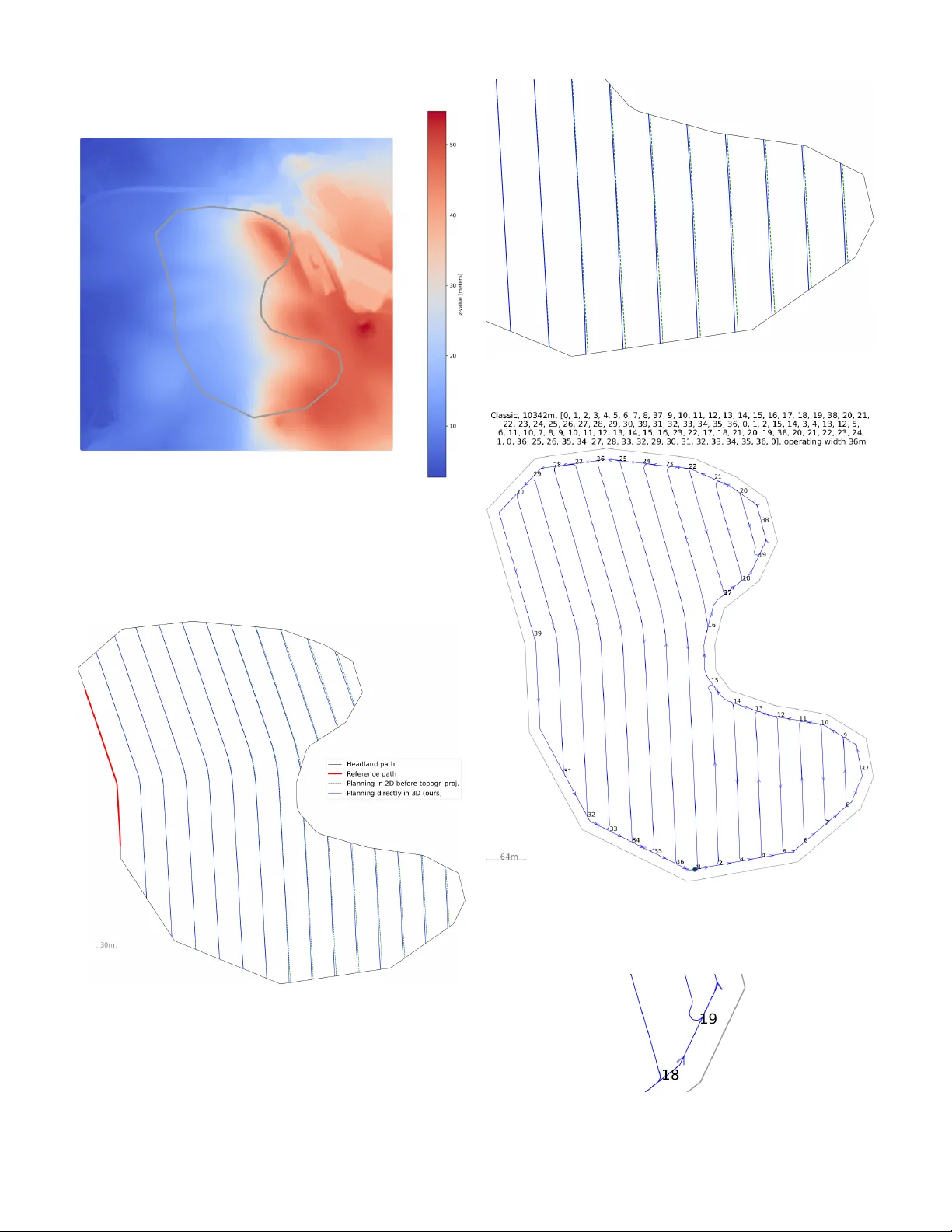
Fr om 2D to 3D terrain-f ollo wing ar ea cov erage path planning Mogens Plessen* Abstract —An algorithm for 3D terrain-following ar ea coverage path planning is pr esented. Multiple adjacent paths ar e generated that are (i) locally apart from each other by a distance equal to the working width of a machinery , while (ii) simultaneously floating at a projection distance equal to a specific working height abov e the terrain. The complexities of the algorithm in comparison to its 2D equivalent are highlighted. These include uniformly spaced elevation data generation using an In verse Dis- tance W eighting-appr oach and a local search. Area coverage path planning results for real-world 3D data within an agricultural context are pr esented to validate the algorithm. Index T erms —3D area co verage path planning, agriculture. I . I N T RO D U C T I O N Agricultural real-world terrain is rarely completely flat. Therefore, 3D terrain data have to ideally be accounted for to generate precision paths for autonomous robotic area coverage path planning. F or robots that operate within a field or work area with a specific working width and height, e.g. for spraying applications where nozzles are attached along a boombar that is carried by a vehicle at a specific working height above the terrain (boom height), area cov erage paths are sought that do neither produce area cov erage gaps nor overlaps. 3D area coverage path planning is titularly not a ne w topic. Howe v er , a literature re view rev ealed that there existed a research gap for a method that generates multiple adjacent paths that are (i) locally apart from each other by a distance equal to the working width of a machinery (e.g., the boombar width), while (ii) at the same time floating at each sampling point at a projection distance equal to a specific working height (e.g., the boom height) abov e the terrain. The presentation of such an algorithm is the contribution of this paper . T o the best of the author’ s knowledge this is for ground- based v ehicles the first paper that presents an area cov erage planning method ov er 3D terrain that simultaneously accounts for a specific working width and also w orking height. For interest and extension, the standard commercial ap- proach for area coverage path planning for uncrewed aerial ve- hicles (U A V) in agriculture is to plan in 2D, before afterwards following the terrain via feedback control height reference tracking. This approach does also not simultaneously account for working width and height during the area coverage path planning step. The remaining paper focuses exclusiv ely on the case for ground-based vehicles. A literature revie w is provided. The standard approach to e xtend 2D area co verage path planning methods to the 3D case is to plan in 2D before projecting the path onto the terrain via a Digital Elev ation Model (DEM) that maps, e.g., latitude and longitude coordinates to elev ation coordinates. Ho we ver , while on the latitude-longitude lev el two adjacent paths may appear parallel to each other for a specific working width, they are not for topographically varying terrain. A plethora of papers exist that maintain this general projection approach but search for an optimal ’ driving direction’ that accounts for 3D terrain data, and often optimize * pmogens@proton.me , Findklein GmbH, Switzerland w (a) V isulization of adjacent paths resulting from the cylindical approach from [1]. Adjacent paths are spaced by a distance w . w > w h h · · (b) The method implicitly assumes a working height of zero. This simplification is in many agricultural applications not merited. E.g., the center-of-gra vity (CoG) of some self-propelled sprayers may be more than 2m above ground. Fig. 1. Illustration of an important disadvantage of the method from [1]. A zero vehicle height is implicitly assumed. While adjacent paths are spaced by nominal working width w along the ground surface, this is not the case anymore as soon as a vehicle height larger than zero, h > 0 , is assumed. boombar Fig. 2. Bird’ s eye view: visualization of the terms headland path , mainfield lane and a v ehicle co vering an area with a working width to spray an area (e.g., pesticide application). T op : Real-world visualization. Bottom : Abstract visualization where a vehicle might tra vel from location Q towards R or D. w h h · · w w terr ain Fig. 3. Goal: area coverage paths floating at a projection distance h above the terrain while adjacent mainfield lanes are spaced by distance w . a multi-objectiv e function inv olving energy consumption [2]– [8]. The search for the optimal dri ving direction is often done stochastically via genetic programming [9]. Multiple papers also propose the partition the field area into se veral subfields to exploit varying terrain characteristics [10]–[12]. Specific path shaping mechanisms were considered. A Fermat spiral path planning method to exploit dif ferent height contour lines is used in [13]. Constraints on trajectory curvature are taken into account via second-order cone programming [14]. Beyond agricultural fields the topic of 3D path planning is also rele vant for lawn mowers [15] and vineyards [16], [17]. Closest to the objecti ve of the present paper is the work of [1], where a ‘ 3D side-to-side cover age algorithm is pr oposed in which spaces between adjacent swaths ar e kept equal taking into account the topogr aphical natur e of the field ’. T o create adjacent swaths it is proposed to (i) create at each sampling point and for a specific heading a cylinder with radius equal to the working width, before (ii) intersecting this cylinder with the 3D topographical surface to obtain the corresponding coordinate of an adjacent swath. This approach, howe ver , has an important disadv antage. It implicitly assumed a zero vehicle height. See Fig. 1 for visualization. The remaining paper is or ganized as follo ws: problem formulation, problem solution, numerical examples, discussion and the conclusion are described in Sect. I-VI. I I . P RO B L E M F O R M U L AT I O N A robot with a working width (boombar width) of w is assumed to be operating in an agricultural field or , more gen- erally , a specific work area. The boombar shall be maintained at a nominal boom height h abo ve the terrain. Efficient path plans are desired for full area co verage. Planning in 2D, typically based on latitude and longitude data, implicitly assumes a flat terrain. When tracking a 2D area cov erage path plan in real-world non-planar terrain, spray gaps result. One solution to a void spray gaps while maintaining a 2D planning technique is to determine the maximum spray gap distance from data, reducing the ef fectiv e working width by this distance, before recalculating a ne w area cov erage path plan for this effecti ve (instead of the original) working width. While the resulting path would not generate any spray gaps, howe ver , instead no w spray overlaps would result. Thus, to minimize both spray gaps as well as overlaps it has to be accounted for 3D terrain data directly during area coverage path planning. T o provide such a method is the problem addressed in this paper . See Fig. 2 and 3 for illustration. Note that partial field coverage (e.g., as a result of ac- counting for varying spray tank level dynamics during field operations) and the like are not of concern for this paper , where the focus is on providing a mathematical algorithm to compute area coverage paths accounting for 3D terrain data. I I I . P RO B L E M S O L U T I O N Let 3D position coordinates be denoted in the classic three-dimensional Cartesian coordinate system by ( x, y , z ) ∈ R 3 , where the z -coordinate denotes elev ation. Let β j ∈ ( − π / 2 , π/ 2) for j ∈ { left , right } denote the angles of the boombar with respect to sea-lev el ( x − y plane) on the left and right-hand side of the center of the boombar , respectiv ely . It is assumed that these angles can be controlled independently . See Fig. 4 for illustration. Let ∆ h ( b ) > 0 , ∀ b ∈ [ − w / 2 , w/ 2] w h h · · w w terr ain β left β right Fig. 4. (i) V ehicle visualization, and (ii) illustration of the assumption that boombar halves can be controlled independently up to a specific angle. The control of two boombar halves over two adjacent paths enables full working width w . w h h α α β r = w · γ z Fig. 5. V isualization of variables used in the Algorithm of Sect. III-B. denote the boom height with respect to the terrain as a function of position b along the boombar . The core necessity for efficient area co verage path planning is to generate sub-paths, here called mainfield lanes (see Fig. 2) that are locally minimizing (and ideally eliminating) both spray gaps as well as overlaps. In agriculture, where the work area is typically di vided into a headland area used for turning and a mainfield area, this concept is predominantly important for the path planning of mainfield lanes. Howe ver , it may also be rele vant for headland area paths, e.g., if multiple adjacent headland paths are planned. T o summarize, the main difficulty for 3D terrain-follo wing area coverage path planning is to efficiently generate locally adjacent paths that maintain a distance of the working width w to each other, while accounting for a working height h and the 3D terrain. Note that once a 3D lane grid is created that connects all mainfield lanes and headland paths, a graph optimization can be solved applying the exact same techniques as for 2D area cov erage path planning (e.g. [18]). A. Generating adjacent paths in 3D terrain In the follo wing a method is described to generate adjacent mainfield lanes for area coverage path planning along 3D terrain. Assume a 3D reference path (e.g., a previously gen- erated mainfield lane) is av ailable, { ( x ( k ) i , y ( k ) i , z ( k ) i ) } N ( k ) i =0 , that is described by an ordered sequence of N ( k ) > 0 coordinates and where the mainfield lane number shall be index ed by k > 0 . An adjacent mainfield lane path, { ( x ( k +1) i , y ( k +1) i , z ( k +1) i ) } N ( k +1) i =0 , is sought. Concatenating multiple of such adjacent lanes shall produce area coverage, while minimizing spray gaps as well as overlaps along 3D terrain. The 3D terrain is assumed to be av ailable in the form of a look-up table in combination with an interpolation routine that maps ( x, y ) -coordinates to ele vation, z = f ( x, y ) , ∀ x ∈ X , y ∈ Y , where X and Y denote the x - and y -coordinate ranges relev ant for a giv en field area, respectiv ely . The con- struction of an efficient look-up table is discussed further below in Sect. III-D. B. Algorithm For each coordinate along mainfield lane k , the follo wing calculations are computed. First, ψ ( k ) i = arctan( y ( k ) i +1 − y ( k ) i x ( k ) i +1 − x ( k ) i ) , (1a)     x ( k ) i, ( m ) y ( k ) i, ( m ) z ( k ) i, ( m )     = 1 2    x ( k ) i + x ( k ) i +1 y ( k ) i + y ( k ) i +1 z ( k ) i + z ( k ) i +1    , (1b) Second, if the point (1b) is ele vated at a projection distance of approximately the nominal boom height h above the terrain, set:     x ( k ) i, ( h ) y ( k ) i, ( h ) z ( k ) i, ( h )     =     x ( k ) i, ( m ) y ( k ) i, ( m ) z ( k ) i, ( m )     , (2) else, calculate: " x ( k ) i, ( a ) y ( k ) i, ( a ) # = " x ( k ) i, ( m ) y ( k ) i, ( m ) # + a " cos( ψ ( k ) i + π 2 ) sin( ψ ( k ) i + π 2 ) # , (3a) z ( k ) i, ( a ) = f ( x ( k ) i, ( a ) , y ( k ) i, ( a ) ) , (3b) α ( k ) i, ( a ) = arctan( z ( k ) i, ( m ) − z ( k ) i, ( a ) a ) , (3c) " x ( k ) i, ( h ) y ( k ) i, ( h ) # = " x ( k ) i, ( m ) y ( k ) i, ( m ) # + h sin( α ( k ) i, ( a ) ) " cos( ψ ( k ) i + π 2 ) sin( ψ ( k ) i + π 2 ) # , (3d) z ( k ) i, ( h ) = f ( x ( k ) i, ( m ) , y ( k ) i, ( m ) ) + h cos( α ( k ) i, ( a ) ) , (3e) where a > 0 denotes half of the tractor vehicle’ s axle width. Third, " x ( k +1) i, ( w ) y ( k +1) i, ( w ) # = " x ( k ) i, ( h ) y ( k ) i, ( h ) # + w " cos( ψ ( k ) i + π 2 ) sin( ψ ( k ) i + π 2 ) # , (4a) z ( k +1) i, ( w ) = f ( x ( k +1) i, ( w ) , y ( k +1) i, ( w ) ) , (4b) β ( k +1) i, ( w ) = arctan( z ( k ) i, ( h ) − z ( k +1) i, ( w ) − h w ) , (4c) ˆ w ( k +1) i, ( w ) = w cos( β ( k +1) i, ( w ) ) , (4d) " x ( k +1) i, ( w ) y ( k +1) i, ( w ) # = " x ( k ) i, ( h ) y ( k ) i, ( h ) # + ˆ w ( k +1) i, ( w ) " cos( ψ ( k ) i + π 2 ) sin( ψ ( k ) i + π 2 ) # , (4e) z ( k +1) i, ( w ) = z ( k ) i, ( h ) − w sin( β ( k +1) i, ( w ) ) , (4f) d vert , ( k +1) i, ( w ) = z ( k +1) i, ( w ) − f ( x ( k +1) i, ( w ) , y ( k +1) i, ( w ) ) , (4g) h proj , ( k +1) i, ( w ) = | d vert , ( k +1) i, ( w ) cos( β ( k +1) i, ( w ) ) | , (4h) where h proj , ( k +1) i, ( w ) approximates the projection distance to the terrain. This approximation is done (i) for computational T ABLE I. Hyperparameters used in numerical experiments, including angle stepsize and distance tolerance.. Hyperp. V alue ϵ 0.1 (m) ∆ β 1 (°) efficienc y (to av oid an additional local search), and (ii) is reasonable for typically small roll angles β ( k +1) i, ( w ) . A more accurate alternative would require an additional local search to determine angle γ according to Fig. 5 to calculate the correct projection distance since the terrain is in general arbitrarily locally varying, h proj , ( k +1) i, ( w ) = min x ∈X , y ∈Y , z = f ( x,y ) {||     x ( k +1) i, ( w ) y ( k +1) i, ( w ) z ( k +1) i, ( w )     − " x y z # || 2 } , where the projection distance is calculated using the Euclidean norm. Fourth, if | h proj , ( k +1) i, ( w ) − h | < ϵ , where ϵ > 0 is a hyperpa- rameter small tolerance le vel, return    x ( k +1) i y ( k +1) i z ( k +1) i    =     x ( k +1) i, ( w ) y ( k +1) i, ( w ) z ( k +1) i, ( w )     , (5) else, use a hyperparameter angle, ∆ β > 0 , to adapt β ( k +1) i, ( w ) = ( β ( k +1) i, ( w ) − ∆ β , if h proj , ( k +1) i, ( w ) < h, β ( k +1) i, ( w ) + ∆ β , else , (6) and repeat Steps (4d)-(4h) until, | h proj , ( k +1) i, ( w ) − h | ≤ ϵ , or the tolerance error does not further decrease, and (5) is returned. C. Details and e xtensions Multiple comments are made. First, hyperparameters used in the e valuation experiments are listed in T able I. They are intuitiv e and well interpretable as angle stepsize and distance tolerance. Second, the stopping criterion for the iterations of Steps (4d)-(4h) is specified when the tolerance error does not further decrease. Let h proj , ( k +1) i, ( w ) ( j − 1) and h proj , ( k +1) i, ( w ) ( j ) denote the projection distances at two consecutiv e iteration indices j − 1 and j , respecti vely . Then, if sign ( h proj , ( k +1) i, ( w ) ( j ) − h )  = sign ( h proj , ( k +1) i, ( w ) ( j − 1) − h ) , compute η j = 1 | h proj , ( k +1) i, ( w ) ( j ) − h | , (7a) η j − 1 = 1 | h proj , ( k +1) i, ( w ) ( j − 1) − h | , (7b) β ( k +1) i, ( w ) = η j β ( k +1) i, ( w ) ( j ) + η j − 1 β ( k +1) i, ( w ) ( j − 1) η j + η j − 1 , (7c) ˆ w ( k +1) i, ( w ) = w cos( β ( k +1) i, ( w ) ) , (7d) " x ( k +1) i, ( w ) y ( k +1) i, ( w ) # = " x ( k ) i, ( h ) y ( k ) i, ( h ) # + ˆ w ( k +1) i, ( w ) " cos( ψ ( k ) i + π 2 ) sin( ψ ( k ) i + π 2 ) # , (7e) z ( k +1) i, ( w ) = z ( k ) i, ( h ) − w sin( β ( k +1) i, ( w ) ) , (7f) before terminating and returning the results in (7e) and (7f) as (5). Third, note that as a result of abov e computations adjacent paths result that are locally apart from each other by distance w , while at the same time floating at each sampling point at a projection distance of approximately h abo ve the terrain. Fourth, note that the nominal boom height or projection distance h is enforced (subject to tolerance ϵ ) only at mainfield lane centerlines. There is in general no guarantee that this distance is maintained along the entire width of the boombar . In fact, o ver unev en terrain it is impossible to ensure this along the entire width of the boombar for the general case of arbitrarily locally v arying terrain. This is an important observation. Each left and right boombar half is modeled as a rigid body . W e selected projection distance to be h at the outest boombar tips (i.e., at the CoG mainfield lane paths), respectiv ely . Other design selections, e.g. at the halves of each boombar half are also possible. Finally , during the computation of above Algorithm the condition, | β ( k +1) i, ( w ) | < β max boombar , can be used to exclude area cov erage paths resulting in excessi ve roll angles or roll angles abov e a threshold β max boombar > 0 . If a path with a roll angle exceeding the threshold is detected, a new alternati ve initial reference path (e.g., an alternati ve subsection of the area contour) is selected before the Algorithm of Sect. III-B is restarted. D. Look-up table pr eparation for elevation computation 3D terrain data is assumed to be av ailable in the form of a look-up table. A fast ev aluation of (3b), (3e), (4b) and (4g) is crucial for overall computational efficienc y of above Algorithm. One approach is to organize the look-up table based on a uniform interpolation grid. The steps are as follo ws. First, suppose sampled 3D terrain data is initially av ailable ar- bitrarily non-uniformly spaced, { x j, ( s ) , y j, ( s ) , z j, ( s ) } N ( s ) j =0 , with N ( s ) > 0 data points. Second, decide a hyperparameter interpolation grid spacing, ∆ g > 0 , used for both x - and y -ax es. Third, prepare the look-up table by ev aluating the elev ation along the interpolation grid using an Inver se Distance W eighting (ID W) approach [19], f ( x m , y n ) =    z ⋆, ( m,n ) q , if d ⋆, ( m,n ) q = 0 , P Q IDW q =0 η ⋆, ( m,n ) q z ⋆, ( m,n ) q P Q IDW q =0 η ⋆, ( m,n ) q , else , (8) where η ⋆, ( m,n ) q = 1 d ⋆, ( m,n ) q for d ⋆, ( m,n ) q = q ( x m − x ⋆ q ) 2 + ( y n − y ⋆ q ) 2 , and indices q ∈ { 0 , . . . , Q IDW } indicate the Q IDW + 1 in Euclidean distance measured closest points to the interpolation grid coordinate ( x m , y n ) . In experiments hyperparameters are selected as ∆ g = 1 m and Q IDW = 3 . Once 3D terrain data is a vailable over an uniformly spaced interpolation grid, classic Bilinear Interpolation (BI) can be used to interpolate the elev ation at an arbitrary ( x, y ) - coordinate. Suppose ( x, y ) is within a cell of the uniform interpolation grid, such that x l ≤ x ≤ x u and y l ≤ y ≤ y u and f ( x j , y j ) , ∀ j ∈ { l, u } is available, then f ( x, y ) can be ev aluated as follo ws: f ( x, y l ) = x u − x x u − x l f ( x l , y l ) + x − x l x u − x l f ( x u , y l ) , (9a) f ( x, y u ) = x u − x x u − x l f ( x l , y u ) + x − x l x u − x l f ( x u , y u ) , (9b) f ( x, y ) = y u − y y u − y l f ( x, y l ) + y − y l y u − y l f ( x, y u ) . (9c) Bilinear interpolation cannot be used directly on raw data since it is in general non-uniformly spaced by above assump- tion. This necessitated abov e ID W -step first. E. P ath tang ential interpolation spacing All of above discussion focused on details for the cre- ation of adjacent paths while accounting for 3D terrain data, the working width w and height h . Abov e discussion did not yet address path tangential interpolation spacings, d ( k ) i = q ( x ( k ) i +1 − x ( k ) i ) 2 + ( y ( k ) i +1 − y ( k ) i ) 2 + ( z ( k ) i +1 − z ( k ) i ) 2 , for i = 0 , . . . , N ( k ) coordinates along each of the adjacent paths k = 1 , . . . , K . When generating a cascaded sequence of multiple adjacent paths, the interpolation distance along the first reference path is highly influential on the result of all the adjacent paths. This is since any potential projection errors are accumulated over multiple projections to generate the multiple adjacent paths. Selecting a specific interpolation spacing along the reference path is a heuristic choice. The method suggested in this paper , and used for the numerical experiments in Sect. IV, is (i) based on only 2 parameters, namely working width w and an assumed maximal permissible absolute heading change ∆ ψ max > 0 along the reference path, and (ii) is deriv ed based on geometric argumentation to avoid generation of jaggedness in adjacent paths. The guiding inequality is d sin (∆ ψ max ) + w cos (∆ ψ max ) ≥ w , from which the minimum path tangential interpolation spacing is calculated as, d ≥ w (1 − cos (∆ ψ max )) / sin (∆ ψ max ) . Assuming a maximal permissible ∆ ψ max = 30 ◦ and w ork- ing width w = 36 m, this results in d min ≈ 10 m. In belo w numerical experiments, this interpolation spacing is enforced along the initial reference path. It is underlined that abov e method is one possible heuris- tic. More complex ones, e.g. that also account for height, maximum absolute roll angle assumptions or are fully data- dependent based on (exhaustiv e) terrain searches, are possible. The benefit of above method with only 2 parameters is its simplicity . I V . N U M E R I C A L E X P E R I M E N T S Data used for numerical e xperiments are illustrated in Fig. 6. The results of 2 different methods for the generation of adjacent mainfield lanes while accounting for 3D terrain data are visualized in Fig. 7. A zoom-in in Fig. 8 further highlights the dif ferences of the 2 methods. Only the solution resulting from planning directly in 3D a voids the spray overlap or spray gaps issues that are associated with 2D-planning before path projections onto the topographical map, as outlined in Sect. II. The full 3D terrain-follo wing area cov erage path planning result is shown in Fig. 9. A zoom-in is in provided in Fig. 10 to highlight smooth transitions between mainfield lanes and the headland path. Fig. 6. Illustration of data used for numerical experiments. A field with non- con vex contour (gray) is embedded within a real-world topographical map. The ele vation profile (z-value) ranges from belo w 10m to more than 50m above sea-lev el. The field has a size of 28.6ha. Fig. 7. Creation of mainfield lanes: bird’s eye view comparison of the methods of (i) hierarchically planning first freeform lanes in 2D according to [20] before their projections onto the terrain, and (ii) directly planning mainfield lanes in 3D according to the Algorithm of Sect. III-B. The working width and height are w = 36 m and h = 2 m. The maximum lateral deviation between the results of the 2 methods is 2.83m (see also the zoom-in in Fig. 8). Fig. 8. Zoom-in into the south-eastern part of Fig. 7. The maximum lateral deviation between the results of the 2 methods (dashed and solid) is 2.83m. Fig. 9. Full area coverage path planning result. For the mainfield lanes generated by the 3D-planning approach in Fig. 7, a sequence of mainfield lane trav ersals is assigned before transitions between mainfield lanes and headland path are smoothed according to [21]. The field entry and exit location is indicated by the green 0-node. Fig. 10. A zoom-in into part of Fig. 9. V . D I S C U S S I O N A N D O U T L O O K T errain-following area cov erage planning in 3D is related to 2D freeform path fitting methods (e.g., [20]). Ho wev er, the complexities stemming from the change to non-planar terrain are significant. They result in eqs. (3a)-(3e), (4a)- (4h), and iteration (6) in combination with (4d)-(4h) and (7). The entire look-up table generation step from Sect. III-D and hyperparameters in T able I are also not required for 2D. The method from [1], which was highlighted in the In- troduction, could in general be adapted for the 3D problem discussed in this paper . This adaptation would encompass, (i) projecting the entire terrain locally orthogonal by a distance h , before then (ii) treating this projected surface as the new field surface and applying the c ylindrical method from [1]. Howe ver , this projection step is in general not straightforward, since dependent on interpolation spacing and working height easily jaggedness is introduced into the new surface, whose correction is not straightforw ard. Furthermore, the projection step is inefficient since in general (without the introduction of additional heuristics and hyperparameters) the entire field surface would ha ve to be projected, before the cylindrical method can be applied. There are 3 main avenues for future work. First, head- land path edges and headland-to-mainfield lane transitions are currently smoothed before being vertically projected onto the terrain. For an improv ed method it is planned to use a 3D dynamical tractor model and adapt the method [21] to calculate these transitions. Second, the modeling of terrain data can potentially be improv ed. Instead of using look-up tables, a polynomial fit may be used (e.g., [22], [23]). A trade-off be- tween potentially impro ved computational ef ficiency and loss of 3D terrain modeling accuracy is expected. Third, alternative heuristics for path tangential interpolation spacing (see Sect. III-E) may be re viewed to refine performance guarantees. V I . C O N C L U S I O N An algorithm for the generation of 3D terrain-follo wing area cov erage path planning was presented. Multiple adjacent paths are generated that are (i) locally apart from each other by a distance equal to the working width of a machinery (e.g., the boombar width for agricultural spraying applications), while (ii) at the same time floating at each sampling point at a projection distance equal to a specific height above the terrain (e.g. the boom height or nominal distance of nozzles abov e the ground). The complexities of the algorithm in comparison to its 2D equiv alent are highlighted that arise due to the introduction of the third dimension. These include in particular , a look- up table generation using an In verse Distance W eighting (ID W)-approach to generate elev ation data over a uniform interpolation grid and a local search. R E F E R E N C E S [1] I. A. Hameed, A. la Cour-Harbo, and O. L. Osen, “Side-to-side 3d coverage path planning approach for agricultural robots to minimize skip/overlap areas between swaths, ” Robotics and Autonomous Systems , vol. 76, pp. 36–45, 2016. [2] I. A. Hameed, “Intelligent coverage path planning for agricultural robots and autonomous machines on three-dimensional terrain, ” Jrnl. of Intelligent & Robotic Systems , vol. 74, no. 3, pp. 965–983, 2014. [3] S. Dogru and L. Marques, “Energy efficient coverage path planning for autonomous mobile robots on 3d terrain, ” in Intl. Conf. on Autonomous Robot Systems and Competitions , pp. 118–123, IEEE, 2015. [4] M. Shen, S. W ang, S. W ang, and Y . Su, “Simulation study on coverage path planning of autonomous tasks in hilly farmland based on energy consumption model, ” Mathematical pr oblems in engineering , vol. 2020, no. 1, p. 4535734, 2020. [5] L. Bostelmann-Arp, C. Steup, and S. Mostaghim, “Multi-objective seed curve optimization for coverage path planning in precision farming, ” in Pr oc. of the Genetic and Evolutionary Comput. Conf. , pp. 1312–1320, 2023. [6] M. V ahdanjoo, R. Gislum, and C. G. Sørensen, “Three-dimensional area coverage planning model for robotic application, ” Computers and Electr onics in Agricultur e , vol. 219, pp. 1–15, 2024. [7] H. Jiang and P . Y ang, “ A three-dimensional cov erage path planning method for robots for farmland with complex hilly terrain, ” Applied Sciences , vol. 14, no. 23, p. 11231, 2024. [8] X. Lin, J. Y an, H. Du, and F . Zhou, “Path planning for full co verage of farmland operations in hilly and mountainous areas based on the dung beetle optimization algorithm, ” Applied Sciences , vol. 15, no. 16, p. 9157, 2025. [9] W . Qiu, D. Zhou, W . Hui, A. R. Kwabena, Y . Xing, Y . Qian, Q. Li, H. Pu, and Y . Xie, “T errain-shape-adaptive coverage path planning with trav ersability analysis, ” Jrnl. of Intelligent & Robotic Sys. , vol. 110, no. 1, p. 41, 2024. [10] J. Jin and L. T ang, “Coverage path planning on three-dimensional terrain for arable farming, ” Jrnl. of F ield Robotics , vol. 28, no. 3, pp. 424–440, 2011. [11] T . ˇ Rezn ´ ık, L. Herman, M. Klocov ´ a, F . Leitner, T . P av elka, ˇ S. Leitgeb, K. Trojano v ´ a, R. ˇ Stampach, D. Moshou, A. M. Mouazen, et al. , “T owards the dev elopment and verification of a 3d-based advanced optimized farm machinery trajectory algorithm, ” Sensors , vol. 21, no. 9, p. 2980, 2021. [12] D. Pour Arab, M. Spisser , and C. Essert, “3d hybrid path planning for optimized coverage of agricultural fields: A nov el approach for wheeled robots, ” Jrnl. of F ield Robotics , vol. 42, no. 2, pp. 455–473, 2025. [13] C. W u, C. Dai, X. Gong, Y .-J. Liu, J. W ang, X. D. Gu, and C. C. W ang, “Energy-ef ficient coverage path planning for general terrain surfaces, ” IEEE Robotics and Automation Letters , vol. 4, no. 3, pp. 2584–2591, 2019. [14] T . T ormagov and L. Rapoport, “Coverage path planning for 3d terrain with constraints on trajectory curvature based on second-order cone programming, ” in Intl. Conf. on Optimization and Applications , pp. 258– 272, Springer, 2021. [15] H. Zhou, P . Zhang, Z. Liang, H. Li, and X. Li, “Cov erage trajectory planning problem on 3d terrains with safety constraints for automated lawn mo wer: Exact and heuristic approaches, ” Robotics and Autonomous Systems , p. 105109, 2025. [16] O. Contente, N. Lau, F . Morgado, and R. Morais, “ A path planning application for a mountain vineyard autonomous robot, ” in Robot 2015: Second Iberian Robotics Confer ence: Advances in Robotics, V olume 1 , pp. 347–358, Springer, 2015. [17] L. Santos, N. Ferraz, F . N. dos Santos, J. Mendes, R. Morais, P . Costa, and R. Reis, “Path planning aware of soil compaction for steep slope vineyards, ” in Intl. Conf . on Autonomous Robot Systems and Competi- tions , pp. 250–255, IEEE, 2018. [18] M. G. Plessen, “Optimal in-field routing for full and partial field coverage with arbitrary non-conve x fields and multiple obstacle areas, ” Biosystems engineering , vol. 186, pp. 234–245, 2019. [19] D. Shepard, “ A two-dimensional interpolation function for irregularly- spaced data, ” in Pr oc. of the 1968 23rd ACM national confer ence , pp. 517–524, 1968. [20] M. G. Plessen, “Freeform path fitting for the minimisation of the number of transitions between headland path and interior lanes within agricultural fields, ” Artificial Intelligence in Agricultur e , vol. 5, pp. 233– 239, 2021. [21] M. Plessen, “Smoothing of headland path edges and headland-to- mainfield lane transitions based on a spatial domain transformation and linear programming, ” Biosystems Engineering , vol. 257, p. 104229, 2025. [22] M. M. Blane, Z. Lei, H. Civi, and D. B. Cooper, “The 3l algorithm for fitting implicit polynomial curves and surfaces to data, ” IEEE T rans. on P attern Analysis and Machine Intelligence , vol. 22, no. 3, pp. 298–313, 2002. [23] J. C. Carr , R. K. Beatson, J. B. Cherrie, T . J. Mitchell, W . R. Fright, B. C. McCallum, and T . R. Evans, “Reconstruction and representation of 3d objects with radial basis functions, ” in Proceedings of the 28th annual confer ence on Computer graphics and inter active techniques , pp. 67–76, 2001.