A Stable Neural Statistical Dependence Estimator for Autoencoder Feature Analysis

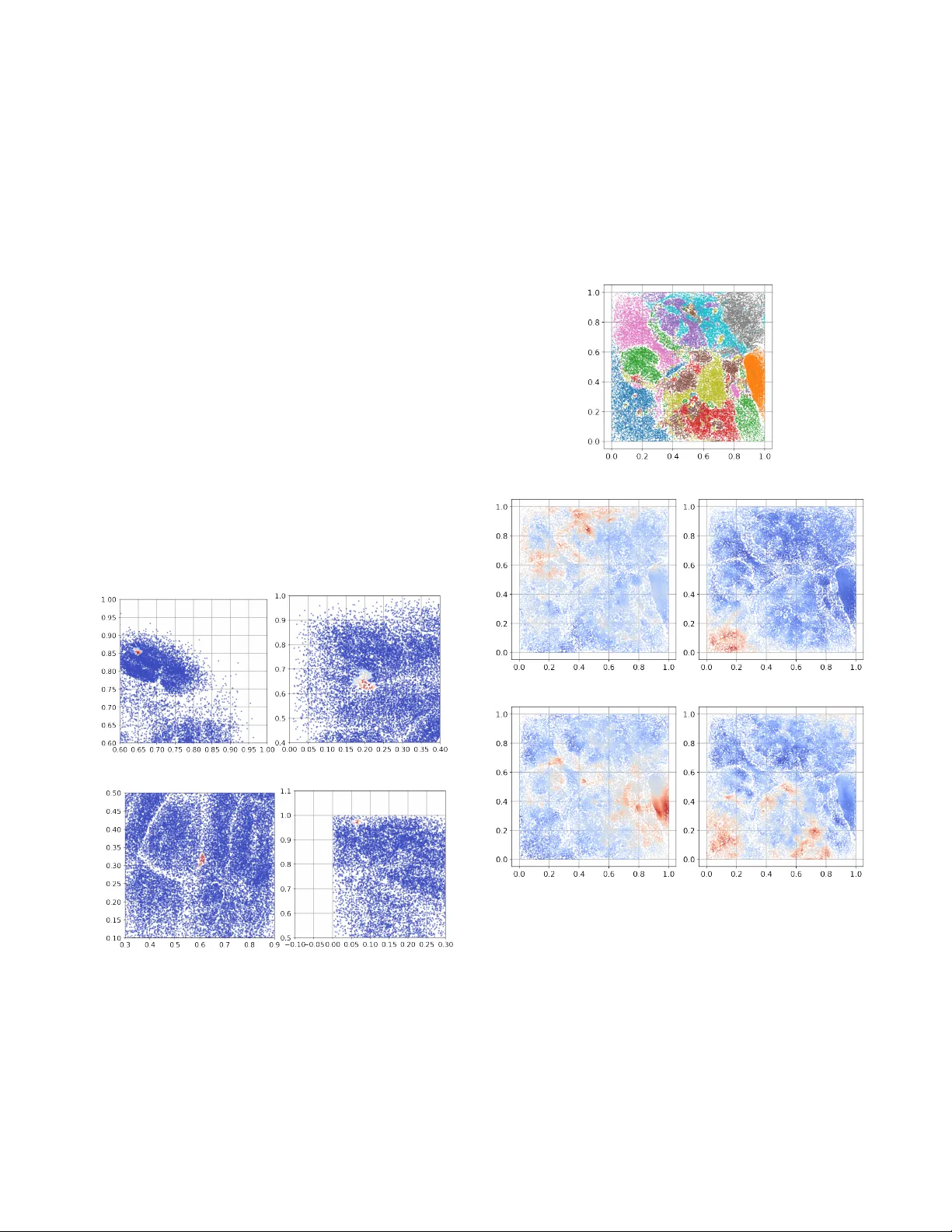
A ST ABLE NEURAL ST A TISTICAL DEPENDENCE ESTIMA T OR FOR A UTOENCODER FEA TURE AN AL YSIS Bo Hu, J osé C. Príncipe Department of Electrical and Computer Engineering Uni versity of Florida hubo@ufl.edu principe@cnel.ufl.edu ABSTRA CT Statistical dependence measures like mutual information is ideal for analyzing autoencoders, b ut it can be ill-posed for deterministic, static, noise-free networks. W e adopt the v aria- tional (Gaussian) formulation that makes dependence among inputs, latents, and reconstructions measurable, and we pro- pose a stable neural dependence estimator based on an or- thonormal density-ratio decomposition. Unlike MINE, our method av oids input concatenation and product-of-marginals re-pairing, reducing computational cost and improving sta- bility . W e introduce an efﬁcient NMF-like scalar cost and demonstrate empirically that assuming Gaussian noise to form an auxiliary v ariable enables meaningful dependence mea- surements and supports quantitati ve feature analysis, with a sequential con vergence of singular v alues. 1. INTR ODUCTION The application of statistical dependence measures to analyze autoencoders is important but technically challenging. Statisti- cal dependence measures, most notably mutual information, quantify uncertainty and the statistical relationships between two random v ariables. Applying such measures to analyze a cascaded encoder-decoder structure has been common in communication systems and information theory [ 1 , 2 ]. Thus, it is natural to apply statistical dependence measures to analyze an autoencoder structure. Another well-established result is that, for a cascaded structure like an autoencoder , minimizing the Mean-Squared Error (MSE) between the input and the output variables amounts to maximizing the statistical dependence, particularly the mutual information, between the input and the intermediate variables [ 3 , 4 ]. Howe ver , we ﬁnd the central obstacle to be that, for a static end-to-end neural network, the statistical dependence between its input and output variables is undeﬁned and not measur- able when no noise is assumed or present. Directly applying an estimator to a deterministic end-to-end neural network is therefore generally ill-posed. The contradiction is that a neural network’ s projection function is deﬁned ov er an actual domain far lar ger than the ﬁnite set of provided dataset samples. Oth- erwise, the netw ork will not hav e generalization capability . A common remedy is the v ariational Bayesian treatment of autoencoders [ 5 , 6 ], in which the encoder and decoder are assumed to parameterize tw o conditional distributions under Gaussian assumptions. W e ﬁnd this assumption generally cor- rect and practically helpful. W e will show that, under this Gaussianity assumption, statistical dependence between in- puts, features, and reconstructions becomes well-deﬁned and can be estimated meaningfully . The obstacle also lies in the stability of the statistical de- pendence estimator . The con ventional procedure of b uilding a statistical dependence estimator often starts with picking a con vex function to deﬁne an f -div ergence, build a v ariational bound for the f -div ergence with the con vex conjugate [ 7 , 8 ] or the Donsker–V aradhan formula [ 9 ], and deriv e a variational cost from this bound such that minimizing this cost will gi ve us estimation of the mutual information. When parameter- ized by a neural network, this approach is typically referred to as the Mutual Information Neural Estimator (MINE) [ 9 ]. In MINE, a neural netw ork f θ is to estimate the density ratio with f θ ( X, Y ) = p ( X,Y ) p ( X ) p ( Y ) , whose inputs are the concatenation of X and Y . It is well known that MINE can be unstable in prac- tice. This paper argues that this instability may come from the parameterization f θ ( X, Y ) . In MINE, the v ariational cost in volves tw o expectations, E X,Y ∼ p ( X,Y ) [ f θ ( X, Y )] and E X,Y ∼ p ( X ) p ( Y ) [ f θ ( X, Y )] . The second expectation requires sample pairs drawn from the product of the marginals, whereas typically we only ha ve sample pairs from the joint. In practice, it is approximated by re-pairing samples within a batch. W ith N joint pairs, naiv e re-pairing will yield N 2 marginal pairs, resulting in high computational complexity and instability . T o address MINE’ s instability , we build on our prior work [ 10 , 11 ] by lev eraging an orthonormal decomposition of the density p ( X,Y ) p ( X ) p ( Y ) = P K k =1 √ λ k · ϕ k ( X ) · ψ k ( Y ) . Instead of approximating the density ratio directly , we learn its left and right singular functions ϕ ( X ) and ψ ( Y ) with neural networks, av oiding input concatenation and eliminating the need for re-pairing. Our previous papers proposed tw o matrix-based costs to learn these functions, based on either matrix in verses or log-determinants. Here we introduce a third alternativ e: a scalar cost similar to Nonne gati ve Matrix Factorization (NMF) that av oids both operations, further improving ef ﬁciency . W e ﬁnd this to be more stable and natural than MINE. Combining the v ariational assumptions for autoencoders with our stabilized dependence estimator , we can gi ve an ac- curate statistical dependence measurement in the autoencoder setting. Beyond feature analysis, we also provide an intuiti ve example of feature learning from the principle of maximiz- ing statistical dependence, although this requires assuming additiv e noise on the data samples. Major result. Our main experimental result shows that, gi ven X and Y , we can construct an auxiliary v ariable X ′ by as- suming additiv e Gaussian noises on X . Although dependence for { X, Y } may be ill-posed to measure in the static setting, dependence for { X ′ , X } and { X ′ , Y } is well-deﬁned and mea- surable. Good features Y should be such that the dependence from { X ′ , X } to { X ′ , Y } does not decay when X is replaced with Y . While this is a compromise relati ve to the noise-free idealization, we ﬁnd it ef fective for quantitati ve analysis and feature learning. 2. OR THONORMAL DECOMPOSITION OF THE DENSITY RA TIO As discussed, our prior work considers approximating the den- sity ratio by its singular functions, rather than approximating it directly . This decomposition is formally described in Eq. ( 1 ) . W e want to approximate the density ratio using the left and right singular functions c ϕ 1 , c ϕ 2 , . . . , c ϕ K and c ψ 1 , c ψ 2 , . . . , c ψ K . The singular v alues √ λ 1 , √ λ 2 , . . . , √ λ K lie in [0 , 1] and in fact a multi variate statistical dependence measure; the y are all zero iff the tw o variables are statistically independent. Since we want to use two neural networks to approxi- mate the top K left and right singular functions, these net- works must be multiple-output. Let f = [ f 1 , f 2 , . . . , f K ] ⊺ and g = [ g 1 , g 2 , . . . , g K ] ⊺ denote their outputs. W e have pre vi- ously identiﬁed two training costs, the log-determinant cost and the trace cost in Eq. ( 2 ) . Both require constructing the autocorrelation matrices R F and R G , as well as the cross- correlation matrix P , by taking expectations of their inner and cross products. Proofs that optimizing these two costs yields the singular functions of the density ratio are provided in the appendix. p ( X, Y ) p ( X ) p ( Y ) = K X k =1 p λ k · c ϕ k ( X ) · c ψ k ( Y ) . (1) (log-det cost) min f , g log det R F G − log det R F − log det R G , (trace cost) max f , g T race ( R − 1 F PR − 1 G P ⊺ ) , R F = E [ f ( X ) f ⊺ ( X )] , R G = E [ g ( Y ) g ⊺ ( Y )] , P = E [ f ( X ) g ⊺ ( Y )] , R F G =  R F P P ⊺ R G  . (2) In this paper , we propose a third alternative. The bottle- necks of the previous costs are the need to compute matrix in- verses and log-determinants. Beyond the SVD, another useful algebraic decomposition is the Nonnegati ve Matrix Factoriza- tion (NMF), which we ﬁnd well suited here as the density ratio is nonnegati ve. Giv en neural networks f = [ f 1 , f 2 , . . . , f K ] ⊺ and g = [ g 1 , g 2 , . . . , g K ] ⊺ , we directly approximate the density ratio as P K k =1 f k ( X ) g k ( Y ) . The functions are no longer required to be orthonormal. Instead, we only impose nonne gati vity , which can be enforced by using a ReLU acti vation in the ﬁnal layer . By the Schwarz inequality , the follo wing inequality will hold:  E h P K k =1 f k ( X ) g k ( Y ) i 2 P K i,j =1 E [ f i ( X ) f j ( X )] · E [ g i ( Y ) g j ( Y )] ≤ Z Z p 2 ( X, Y ) p ( X ) p ( Y ) dX d Y . (3) Deriving this inequality is simple: it follo ws from a direct application of the Schwarz inequality to the inner product ⟨ P K k =1 f k ( X ) g k ( Y ) , p ( X, Y ) ⟩ . For completeness, we pro- vide the full proof in the appendix. W e tak e the left-hand side of inequality ( 3 ) to be our ne w NMF-inspired cost. It is bounded by the mutual information when the con vex function f deﬁning the f -div ergence is cho- sen to be linear , corresponding to Rényi’ s div ergence. W e still compute the autocorrelation matrices R F = E [ f ( X ) f ⊺ ( X )] and R G = E [ g ( Y ) g ⊺ ( Y )] . The denominator of the ne w cost (the left side of the bound ( 3 ) ) is equi valent to P K i,j =1 ( R F ) i,j ( R G ) i,j , or further P K i,j =1 ( R F ⊙ R G ) i,j , where ⊙ denotes the Hadamard (elementwise) product. Here R F and R G are K × K matrices. The ﬁnal cost has the form c =  E h P K k =1 f k ( X ) g k ( Y ) i 2 P K i,j =1 ( R F ⊙ R G ) i,j , or log c. (4) W e w ant to maximize c or log c . A small constant ϵ = 10 − 6 is added to the denominator for stability . This new cost no longer contains matrix in verses or log-determinants nor requires their gradients for the updates. The full algorithm is detailed below . Algorithm 1 Neural NMF for the density ratio. Require: Initialize two neural networks with multiv ariate outputs f = [ f 1 , f 2 , · · · , f K ] ⊺ and g = [ g 1 , g 2 , · · · , g K ] ⊺ . The outputs must be nonnegati ve, so the ﬁnal activ ation layer can be ReLU. At each iteration do: 1: Pass X 1 , X 2 , · · · , X N through netw ork f to obtain f ( X 1 ) , f ( X 2 ) , · · · , f ( X N ) ; 2: Pass Y 1 , Y 2 , · · · , Y N through network g to obtain g ( Y 1 ) , g ( Y 2 ) , · · · , g ( Y N ) ; 3: Compute R F = E [ f ( X ) f ⊺ ( X )] and R G = E [ g ( Y ) g ⊺ ( Y )] using the corresponding networks; compute the joint e xpectation E h P K k =1 f k ( X ) g k ( Y ) i using both networks; 4: Construct and maximize the cost in Eq. ( 4 ); Output: A nonnegativ e factorization of the density ratio. If needed, an SVD can be used after training to recov er the singular func- tions and singular values. The same trick may apply to estimating Shannon’ s mutual information via the Donsker–V aradhan formula, but we focus on the L 2 case because of its link to the eigenexpansion. A common critique of our old costs is also the choice of the number of singular functions, the neural network output dimensions, as if this number is too lar ge, the model tends to di ver ge or be biased. But with this new cost, we found that the dimension can be picked to be very lar ge while the training is still stable. 3. APPL YING A ST A TISTICAL DEPENDENCE ESTIMA TOR TO AN A UT OENCODER W e now describe how the proposed measure can be applied to an autoencoder . W e use the notation N ( X ; v ) to denote a regular Gaussian density function with a shared scalar variance v across dimensions. A con ventional variational analysis of the autoencoder starts with the assumption p ( Y | X ) = N ( Y − E ( X ); v p ) and q ( X | Y ) = N ( X − D ( Y ); v q ) . The objective of an autoen- coder , under this assumption, follows max P Y | X , Q X | Y T r ace  diag ( P X ) · P Y | X · log Q X | Y  . (5) max p ( Y | X ) ,p ( X | Y ) Z Z p ( X ) · p ( Y | X ) · log q ( X | Y ) dX d Y . (6) W e ﬁnd it alw ays helpful for analytical purposes to write do wn the discrete equi valence of an autoencoder (Eq. ( 5 ) ), where P Y | X , Q X | Y are Marko v transition matrices. Our main fo- cus, ho wev er, is the continuous formulation in Eq. ( 6 ) : we sample from the data distribution p ( X ) , pass samples through an encoder p ( Y | X ) = N ( Y ; E ( X ) , v p ) , and then a decoder q ( X | Y ) = N ( X ; D ( Y ) , v q ) . The useful property of this ob- jectiv e is that taking log q ( X | Y ) cancels the exponential term in the Gaussian density , reducing the reconstruction term to just the MSE. A naiv e but important bound is to apply the nonnegati vity of the conditional KL div ergence: Z Z p ( X ) · p ( Y | X ) · log q ( X | Y ) dX d Y ≤ Z Z p ( X ) · p ( Y | X ) · log p ( X | Y ) dX d Y = MI ( X ; Y ) − H ( X ) . (7) It shows that the optimality condition is met when the decoder q is an in verse mapping of the encoder p , such that q ( X | Y ) = p ( Y | X ) . When this condition is satisﬁed, the cost can be written as the mutual information MI ( X ; Y ) minus the data entropy H ( X ) . Note that we seek the maximum v alue of the objectiv e, which means that ev en after the decoder becomes an in verse mapping of the encoder , we must still ﬁnd the Y that maximizes the mutual information with X . This shows why the statistical dependence measure is needed. The v ariational treatment of autoencoders deﬁnes two joint densities: p ( X, Y ) for the encoder and q ( X , Y ) for the de- coder . W e know that q is intended to be an inv erse mapping of p , and that the statistical dependence of p ( X, Y ) is encouraged to be maximized. Our goal is then to measure the statistical dependence of these joint densities. These variances are not directly computable, but can only be estimated. The hidden dilemma here is therefore in fact ho w to set the two noise variances, v p for the encoder and v q for the decoder , or what their true values are. Our arguments are as follo ws. Pick the implicit v q . For the decoder v ariance v q for the reconstructions, we argue that e ven when the static network is trained noise-free, in fact, the optimal decode r variance v q is exactly the empirical v alue of the MSE. When v q is included, the autoencoder objectiv e (Eq. ( 6 ) ) is a Gaussian neg ativ e log-likelihood: it is the squared recon- struction error scaled by v q , plus the normalization terms of the Gaussian: ae _ obj = L 2 · (log 2 π + log v q ) + RR || X − D ( Y ) || 2 2 p ( X, Y ) dX d Y 2 v q . (8) The autoencoder minimizes this. In practice, we often drop the scaling and normalizing constants, and optimize only the reconstruction MSE in the numerator . But if we do care about v q , let us take the deriv ativ e of this objectiv e ae _ obj with respect to the variance v q , and set it to zero: ∂ ae _ obj ∂ v q = L 2 v q − RR || X − D ( Y ) || 2 2 p ( X, Y ) dX d Y 2 v 2 q = 0 , v q = 1 L Z Z || X − D ( Y ) || 2 2 p ( X, Y ) dX d Y . (9) Therefore, the optimal variance v q for a certain MSE value is the MSE value itself. If we minimize the MSE while ignoring v q , then after training we can simply set v q to the current (or ﬁnal optimal) MSE v alue. Minimizing the reconstruction error can be viewed as shrinking the Gaussian balls: the smaller the error , the smaller the radius of these Gaussian balls. Pick the implicit v p . Retrie ving the encoder variance v p is much more dif ﬁcult. The question is posed as follo ws. If we train a static noise-free autoencoder , empirically , the intermedi- ate Y should not hav e any external noise. But the assumption requires p ( Y | X ) = N ( Y − E ( X ); v p ) to be parameterized as a Gaussian. So when we want to measure the statistical dependence, we need to handle this mismatch. Our empirical conclusion in this paper is that the this noise variance v p is at a lev el of 10 − 4 to 10 − 5 for toy datasets and a sigmoid acti vation, and may exist when the setting is static without additi ve Gaussian noises. The evidence is empirical, and comes from the following fe w angles. First, if we train a standard static autoencoder , it can clearly be observed that con vergence has stages: there is a noticeable transition in which the reconstructions and the learned feature boundaries appear coarse at ﬁrst, and then become more and more ﬁne-grained as training progresses. Now we train an autoencoder with additive noise in the features Y ′ = Y + √ v p · noise like in V AE. W e repeat training multiple times, each time using a dif ferent (and progressi vely smaller) v p . Across these runs, the reconstructions again ex- hibit a transition from coarse to ﬁne-grained as v p decreases. This suggests that ev en in the nominally static setting, an ef- fectiv e feature variance v p may be present and may implicitly decrease during training. Empirically , the smallest v p that does not af fect reconstruction quality or training error is on the order of 10 − 5 , which may reﬂect the ef fectiv e v p in the static case. Second, if we look at the reconstructions when the feature dimension is low and visualize them, they look like a low- dimensional manifold existing in a high dimensional space. In order to create this manifold, there must be continuity in the feature v ariable. And the source of this continuity may come from the implicit Gaussian noises. W e conducted a quantitati ve experiment in a Nyström-style fashion. If the data density for toy examples is giv en in closed form, reasonably , it should be possible to learn p and q in a non-empirical way , not from empirical data, b ut by operating directly on the probability density . Thus, we parameterize the encoder and decoder directly with two Mark ov transition matrices, without neural networks. W e found that Gaussian assumptions are required for this non-empirical approach to match the results of an autoencoder . Sweeping over v p , we found that the closest match occurs when v p is at a lev el of 10 − 5 . The third piece of evidence is that, in statistical dependence estimation, assuming the reconstruction variance v q without as- suming the feature variance v p makes the estimation unstable. W ithout v p , we found that the dependence estimation between data samples and reconstructions is stable, b ut the estimation between features and reconstructions is not. After adding the feature noise (i.e., assuming v p ), the estimation becomes more stable. The intrinsic v p for a regular autoencoder , while still requiring further research, could be around 10 − 8 or 10 − 9 . Details of these in vestigations are giv en in the appendix. Our ﬁndings. After selecting v p and v q , we apply statistical dependence estimators to a trained autoencoder to measure the statistical dependence between the inputs, the intermediate features, and the reconstructions. The following notations are used: • X : data samples; • Y : the outputs from passing data samples through the static encoder (features); • Y ′ : Y ′ = Y + √ v p · noise , features Y with additiv e noise; • c X : the outputs obtained from passing the noisy Y ′ through the static decoder (reconstructions); • d X ′ : d X ′ = c X + √ v q · noise , reconstructions c X with additiv e noise. W ith X , Y , Y ′ , c X , and d X ′ , we can measure the statistical de- pendence between any pair of them, and generate a meaningful measurement. Our ﬁndings can be summarized below: 1. { X , Y } and { Y ′ , c X } : measuring dependence between the input and the output of a static network is ill-posed. During training, the estimate increases without bound and div erge. 2. { X , Y ′ } and { Y , Y ′ } : the dependence between X and the noise-corrupted Y ′ is well-deﬁned and can be meaning- fully estimated. Further , it coincides with the dependence between Y and Y ′ , i.e., between the feature and its noise- corrupted version. 3. { Y ′ , d X ′ } and { c X , d X ′ } : similarly , we can meaningfully estimate the dependence between Y ′ and noise-corrupted c X ′ , but not between Y ′ and noise-free c X . The measure- ment value for these tw o pairs are equal. This raises the point that in a static neural network, a mean- ingful measurement of the statistical dependence requires the Gaussianity assumption. The pair { Y , Y ′ } is simple, since Y is the feature and Y ′ is its noise-corrupted version. The pair { X, Y ′ } is complex, since X is high-dimensional data and Y ′ is the projected fea- ture with noises. Despite this difference in complexity , they hav e the same statistical dependence value. The same anal- ysis applies to the d ecoder side for the pairs { Y ′ , d X ′ } and { c X , d X ′ } : when X is substituted by Y , the dependence does not decay . 4. EXPERIMENTS Datasets. W e conduct e xperiments on two datasets: a tw o- moons toy dataset (visualized in Fig. 10 ) and the standard MNIST handwritten digit dataset. Four neural networks are required: an encoder , a decoder , and two dependence-estimator networks. Baselines and parameters. T o demonstrate the effecti veness of our dependence estimator , we compare against three groups. (i) W e contrast our ne w NMF-like scalar cost ( NMF-DR ) with our previous logdet and trace costs ( LOGDET , TRA CE ). (ii) W e include standard MINE estimating Shannon mutual infor - mation ( MINE ). (iii) W e also report kernel-based dependence measures, including KDE , KICA [ 12 ], and HSIC [ 13 ]. Our main emphasis is on (i) and (ii); kernel methods are reported for reference and are not intended as state-of-the-art or practical baselines. All details can be found in the appendix. Ke y hyperparameters are as follo ws. Unless stated oth- erwise, the encoder projects data into 1D features . W e also report higher-dimensional features and sweep this dimension for MNIST (T able 4 ). For decomposition costs, we need to set the estimator output dimension (number of singular functions). It is ﬁxed to be 2000 for the ne w NMF-like cost. For the trace and logdet costs, we use 50 , except for the four cases noted in T able 2 , where we use 500 ; values abo ve 500 are very costly . If this decoder dimension is much larger than the number of positi ve singular v alues, trace and logdet sho w an unwanted bias, while the NMF-like cost does not. W e perturb the features with noise as Y ′ = Y + √ v p · noise and set v p = 10 − 4 . W e also sweep v p in T able 3 and 7 . Result 1. Direct comparisons are reported in T able 1 (two- moon) and T able 2 (MNIST). First, we guarantee that ours three costs yield the same unbiased estimate of Rényi mutual information across v ariable pairs, while NMF-DR is the most efﬁcient and scalable. Second, we observ e consistent equi valences in dependence: the pairs { X, Y ′ } and { Y , Y ′ } are close, and so are { Y ′ , c X ′ } and { c X , c X ′ } , whereas { X, c X ′ } is the lowest. Overall,the y suggest a clear substitution pattern: the original data X can be replaced by the noise-free features Y without changing the dependence, and the noise-corrupted features Y ′ (input to the decoder) and the noise-free reconstruction c X (output of the decoder) are also interchangeable. The encoder-side dependence is consistent across datasets (approximately 28 for 1D features at v p = 10 − 4 ), whereas the decoder-side dependence varies with the data dimension. A notable implication is that the dependence between the data X and the reconstruction c X equals that between noise- free features Y and noisy features Y ′ , because the observed equiv alences allow us to substitute X by Y and c X by Y ′ . MINE does not rev eal such patterns. Encoder pairs Decoder pairs End-to-end Objective ( X , Y ′ ) ( Y , Y ′ ) ( Y ′ , c X ′ ) ( c X , c X ′ ) ( X, c X ) ( X, c X ′ ) NMF-DR 28.57 28.68 22.37 22.38 28.64 16.58 LOGDET 28.35 28.60 22.35 22.36 28.34 16.72 TRA CE 28.46 28.66 22.40 22.40 28.44 19.59* MINE 2.84 3.17 2.63 2.81 2.96 2.36 KDE 20.48 20.57 17.94 20.29 23.22 15.78 KICA 10.99 16.52 10.43 16.45 17.74 12.36 HSIC 10.33 10.78 10.04 18.04 19.03 15.02 *For the trace cost, if the estimator output dimension far e xceeds the number of positiv e singular values, it may introduce an unw anted bias. T able 1 : T wo-moon dataset: measurement comparisons. Encoder pairs Decoder pairs End-to-end Objective ( X , Y ′ ) ( Y , Y ′ ) ( Y ′ , c X ′ ) ( c X , c X ′ ) ( X, c X ) ( X, c X ′ ) NMF-DR 28.81 28.85 200.74 207.90 28.81 28.51 LOGDET 27.98 28.04 199.30* 200.75* 27.98 27.70 TRA CE 28.28 28.34 201.10* 206.97* 28.29 28.02 MINE 1.85 2.09 3.31 4.90 2.07 2.07 KDE 2.50 3.18 3.18 4.93 3.00 2.96 KICA 9.43 16.87 9.47 276.15 270.89 344.04 HSIC 11.62 10.89 11.68 410.93 404.82 495.02 *W e need to increase the estimator output dimension to 500 in these cases. T able 2 : MNIST : measurement comparisons. Result 2. Learning curves are sho wn in Fig. 1 for our costs and in Fig. 2 for MINE. Our costs learn more smoothly and stably , since we a void MINE’ s re-pairing step used for sampling from the product of marginals. (a) T wo-moon curves (b) MNIST (4 curves) (c) MNIST (2 curves) Fig. 1 : Learning curves for the NMF-like cost. The curv es are smooth and stable because no re-pairing is required. Fig. 2 : A learning curve of MINE on MNIST . The sudden “dip” in the curv e is lar gely due to the re-pairing step for sampling from the product of mar ginals. The learning curve would be smoother if we lo wered the learning rate, but con ver - gence would take signiﬁcantly longer . Result 3. The previous experiments ﬁx the feature-noise v ari- ance v p = 10 − 4 . For completeness, we sweep v p from 10 − 7 to 10 − 1 : results for two-moon are reported in T able 3 , and for MNIST in Appendix T able 7 . As the noise level increases, the MSE increases (performance degrades) and the estimated de- pendence decays. Howe ver , the substitution pattern discussed abov e still holds across the sweep. W e can guarantee that in this example the estimator is unbiased. v p MSE Encoder pairs Decoder pairs End-to-end ( × 10 − 3 ) ( X, Y ′ ) ( Y , Y ′ ) ( Y ′ , c X ′ ) ( c X , c X ′ ) ( X, c X ) ( X, c X ′ ) 10 − 7 0.540 519.68 509.61 46.55 46.79 506.74 45.84 10 − 6 0.624 213.59 212.88 40.05 40.25 216.28 37.45 10 − 5 0.650 86.87 87.25 38.71 38.84 87.06 31.90 10 − 4 1.10 28.78 28.83 20.49 20.52 28.80 15.37 10 − 3 2.46 9.82 9.82 9.03 9.04 9.82 6.69 10 − 2 7.18 3.77 3.77 3.76 3.76 3.77 2.73 10 − 1 14.6 1.85 1.85 1.83 1.83 1.85 1.54 T able 3 : T wo-moon: dependence vs. noise levels (NMF-like). Result 4. The previous experiments ﬁx the feature dimension to 1D (the encoder maps the data to a 1D features). W e now sweep it. This is uninformative for two-moon due to its low data dimension, so we report MNIST results. As the feature dimension increases, the MSE decreases and the estimated dependence increases for all variable pairs. The substitution pattern remains. W e can only guarantee unbiased, accurate estimates up to dimension 3, since the total number of used singular functions is capped by the decoder output dimension (2000). Fea. Dim. MSE Encoder pairs Decoder pairs End-to-end ( X, Y ′ ) ( Y , Y ′ ) ( Y ′ , c X ′ ) ( c X , c X ′ ) ( X , c X ) ( X , c X ′ ) 1 0.048 28.81 28.85 200.74 207.90 28.81 28.51 2 0.030 648.40 675.31 1632.26 1661.05 647.28 634.45 3 0.021 1604.27 1679.04 1859.84 1819.99 1576.40 1623.15 4 0.016 1886.03 1885.60 1899.80 1839.93 1846.92 1857.05 5 0.012 1929.32 1875.47 1914.92 1840.91 1892.85 1886.75 T able 4 : MNIST : dependence vs. feature dims (NMF-like). 5. CONCLUSION The experiments we sho w demonstrate that we can go beyond end-to-end mean-squared error , giving statistical dependence measures among many autoencoder components such as data, features, and reconstructions, under a Gaussian assumption. The experiments here are only a fraction of the full set. The appendix will continue with additional experiments. Refer ences [1] Xiangxiang Xu and Lizhong Zheng. Neural feature learn- ing in function space. J ournal of Machine Learning Resear ch , 25(142):1–76, 2024. [2] Ravid Shwartz-Zi v , Randall Balestriero, K enji Kawaguchi, T im GJ Rudner , and Y ann LeCun. An information-theoretic perspecti ve on v ariance- in variance-cov ariance regularization. arXiv pr eprint arXiv:2303.00633 , 2023. [3] Xi Chen, Y an Duan, Rein Houthooft, John Schulman, Ilya Sutske ver , and Pieter Abbeel. Infogan: Interpretable representation learning by information maximizing gen- erativ e adversarial nets. Advances in neur al information pr ocessing systems , 29, 2016. [4] Xiangxiang Xu, Shao-Lun Huang, Lizhong Zheng, and Gregory W W ornell. An information theoretic interpreta- tion to deep neural networks. Entr opy , 24(1):135, 2022. [5] Diederik P Kingma and Max W elling. Auto-encoding variat ional bayes. arXiv pr eprint arXiv:1312.6114 , 2013. [6] Romain Lopez, Jef f rey Re gier, Michael I Jordan, and Nir Y osef. Information constraints on auto-encoding varia- tional bayes. Advances in neural information pr ocessing systems , 31, 2018. [7] XuanLong Nguyen, Martin J W ainwright, and Michael I Jordan. On surrogate loss functions and f-div ergences. The Annals of Statistics , 37(2):876–904, 2009. [8] XuanLong Nguyen, Martin J W ainwright, and Michael I Jordan. Estimating diver gence functionals and the likeli- hood ratio by con vex risk minimization. IEEE T ransac- tions on Information Theory , 56(11):5847–5861, 2010. [9] Mohamed Ishmael Belghazi, Aristide Baratin, Sai Ra- jeswar , Sherjil Ozair , Y oshua Bengio, Aaron Courville, and R. De von Hjelm. Mine: Mutual information neural estimation. In Pr oceedings of the 35th International Con- fer ence on Mac hine Learning (ICML 2018) , volume 80, pages 531–540, 2018. [10] Shihan Ma, Bo Hu, T ianyu Jia, Ale xander Clarke, Blanka Zicher , Arnault Caillet, Dario F arina, and José C Príncipe. Learning cortico-muscular dependence through orthonor - mal decomposition of density ratios. Advances in Neu- ral Information Pr ocessing Systems , 37:129303–129328, 2024. [11] Bo Hu, Y uheng Bu, and José C Príncipe. Learning or- thonormal features in self-supervised learning using func- tional maximal correlation. In 2024 IEEE International Confer ence on Imag e Pr ocessing (ICIP) , pages 472–478. IEEE, 2024. [12] Francis R Bach and Michael I Jordan. Kernel indepen- dent component analysis. Journal of mac hine learning r esearc h , 3(Jul):1–48, 2002. [13] Arthur Gretton, Oli vier Bousquet, Ale x Smola, and Bern- hard Schölkopf. Measuring statistical dependence with Hilbert-Schmidt norms. In International Confer ence on Algorithmic Learning Theory , pages 63–77. Springer , 2005. A. EXTENDED EXPERIMENT AL RESUL TS A.1. Extra tables First, we present a fe w additional tables that continue from the results reported in the main text. Result 5. W e ha ve shown a consistent pattern: smaller Gaus- sian variance corresponds to smaller MSE and higher statistical dependence. This suggests a conjugated relationship among Gaussian variance, MSE, and statistical dependence. During autoencoder training, the cost minimizes the MSE. At each iteration, the current MSE can be interpreted as in- ducing an effecti ve (optimal) Gaussian radius for the recon- structions. As training progresses and the MSE decreases, these Gaussian balls shrink, and the statistical dependence increases. This motivates the question of whether a similar “ball-shrinking” process also occurs for the features, not just the reconstructions. T o in vestigate this, we stop training at 100, 200, 300, 400, 500, and 600 iterations. At each checkpoint, we measure the statistical dependence values for all pairs and examine whether any patterns emerge. T able 5 corresponds to the two-moons dataset, and T able 6 corresponds to MNIST . Iters MSE Encoder pairs Decoder pairs End-to-end × 10 2 × 10 − 3 ( X, Y ′ ) ( Y , Y ′ ) ( Y ′ , c X ′ ) ( c X , c X ′ ) ( X , c X ) ( X , c X ′ ) 0 32.0 0.997 0.998 0.997 0.997 0.997 0.997 1 1.88 23.10 24.03 9.39 9.49 23.24 8.38 2 1.64 24.20 24.94 13.26 13.44 24.98 11.27 3 1.56 24.16 25.29 13.98 14.24 25.42 11.83 4 1.47 24.68 25.50 14.66 14.97 25.46 12.23 5 1.40 25.01 25.43 15.08 15.45 25.77 12.54 6 1.37 24.98 25.68 15.07 15.39 25.79 12.46 T able 5 : T wo-moon dataset: dependence vs. iterations. Iters MSE Encoder pairs Decoder pairs End-to-end × 10 2 ( X, Y ′ ) ( Y , Y ′ ) ( Y ′ , c X ′ ) ( c X , c X ′ ) ( X , c X ) ( X , c X ′ ) 0 0.239 0.998 0.997 0.997 0.998 0.997 0.997 1 0.119 25.00 24.96 28.84 28.96 25.00 17.74 2 0.089 27.12 27.06 70.17 71.06 27.06 24.78 3 0.077 28.29 28.25 97.60 99.55 28.26 26.92 4 0.071 28.46 28.45 110.14 113.46 28.44 27.43 5 0.067 28.42 28.34 117.90 122.06 28.38 27.44 6 0.065 28.51 28.50 124.77 129.50 28.49 27.71 T able 6 : MNIST : dependence vs. iterations. First, the substitution pattern, i.e., the equality of the depen- dence values for the rele vant pairs, holds at ev ery training iteration, starting from initialization. Second, the statistical de- pendence increases for all variable pairs as training proceeds, which supports our argument. In other words, although the cost minimizes the end-to-end MSE, the statistical dependence between the data and the learned features, considering the encoder alone, also increases during training. Moreo ver , train- ing begins from a state of statistical independence: the lo wer bound of the cost is 1 , and attaining this lower bound implies statistical independence. In the main text, we presented a sweep over the encoder feature v ariance v p for the toy dataset. W e also performed the same experiment on MNIST . The results are reported in T able 7 . A notable observation is that the encoder-side statistical dependence, which is bounded by v p , is very similar across the toy dataset (T able 3 ) and MNIST (T able 7 ). The corre- sponding values are close despite the dif ferences in dataset characteristics and input dimensionality . This suggests that the encoder-side dependence pairs { X, Y ′ } and { Y , Y ′ } , as well as the reconstruction pair { X, c X } , may be lar gely irrelev ant to the dataset, depending primarily on the feature dimension and the variance parameter v p . v p MSE Encoder pairs Decoder pairs End-to-end ( X, Y ′ ) ( Y , Y ′ ) ( Y ′ , c X ′ ) ( c X , c X ′ ) ( X , c X ) ( X , c X ′ ) 10 − 7 0.035 781.71 723.36 868.93 877.61 762.46 625.97 10 − 6 0.036 275.65 272.43 793.28 840.97 278.31 265.03 10 − 5 0.041 88.56 88.33 387.96 422.73 88.86 86.90 10 − 4 0.046 28.87 28.88 200.74 207.90 28.87 28.87 10 − 3 0.051 9.83 9.83 65.84 67.29 9.83 9.73 10 − 2 0.058 3.77 3.77 21.78 21.95 3.77 3.73 10 − 1 0.063 1.84 1.84 6.96 6.96 1.84 1.81 T able 7 : MNIST : dependence vs. noise le vels. Concatenating noise to the inputs does not work. The pa- per argues that statistical dependence cannot be meaningfully measured in a static, deterministic, noise-free setting. T o make the quantity well-deﬁned, one can assume a small Gaussian ball around the features. A natural alternati ve is to inject noise through the inputs: we concatenate each data sample with ad- ditional dimensions ﬁlled with i.i.d. uniform random noise as inputs to the encoder . W e w onder if this input-noise concate- nation has the same effect as adding Gaussian noise directly to the features. W e compare dependence estimates for two v ariable pairs under three conditions: the static noise-free setting, concate- nated input noise, and additi ve feature noise with variance v p = 10 − 7 . Unfortunately , concatenating input noise does not solve the issue of over -determination: the dependence esti- mates remain essentially identical to the noise-free case and div erge to very large v alues, making it unclear whether the es- timator is biased or simply ill-posed. In contrast, e ven a small additi ve feature noise ( v p = 10 − 7 ) immediately yields smaller , ﬁnite, and measurable dependence v alues, while only slightly degrading reconstruction performance (MSE 0 . 417 → 0 . 424 ). W e suspect that Gaussian noise is still implicitly associ- ated with the nominally noise-free case. The key difference is that this noise is not injected into the model; instead, it exists “outside” the model, assumed rather than explicitly pre- sented, much like the additi ve noise assumed for reconstruc- tions, whose optimal v alue corresponds to the MSE. W ithout such an assumption, there may be no principled way to mea- sure statistical dependence. Learning seeks to shrink the radius of this Gaussian ball. Learning can be vie wed as shrinking the radius of this Gaussian ball. Noise type MSE NMF-like cost MINE ( X, Y ′ ) ( X , c X ) ( X , Y ′ ) ( X , c X ) Concatenated input noise 0.417 1508.45 1793.36 2.83 4.14 No noise 0.417 1507.52 1782.98 4.68 5.45 Additiv e feature noise 10 − 7 0.424 608.29 583.30 4.64 5.20 T able 8 : Concatenating input noise does not solve the issue that the variable pairs are o verly dependent, which essentially makes the dependence unmeasurable. MINE is very unstable and does not produce a meaningful result. A.2. Eigenanalysis In the main paper we primarily report numerical results for the proposed statistical dependence measures. Recall that our method is based on an orthonormal decomposition of the density ratio p ( X,Y ) p ( X ) p ( Y ) = P K k =1 √ λ k · c ϕ k ( X ) · c ψ k ( Y ) . Apart from the statistical dependence measure itself (i.e., the sum of the singular values), the decomposition also comes with singular v alues and singular functions. In this section, we therefore visualize the learned singular spectrum and singular functions. T o e xtract the singular values and singular functions from the trained networks, we need the follo wing steps: 1. Compute correlation matrices. Estimate the autocorrelation matrices R F = E [ f ( X ) f ⊺ ( X )] and R G = E [ g ( Y ) g ⊺ ( Y )] , and the cross-correlation matrix P = E [ f ( X ) g ⊺ ( Y )] . 2. Whiten the estimator network outputs. Normalize the network features with f = R − 1 / 2 F f and g = R − 1 / 2 G g . 3. Recalculate the cross-correlation in the whitened space: P = E  f ( X ) g ⊺ ( Y )  . 4. Perform SVD: P = Q F Λ 1 / 2 Q ⊺ G . 5. Rotations: b f = Q ⊺ F f and b g = Q ⊺ G g . The resulting b f and b g estimates the singular functions of the density ratio. The diagonal entries of Λ 1 / 2 from the SVD of P estimate the leading singular v alues of the density ratio. Formal justiﬁcation is pro vided in the next appendix section. Learning curves of singular values. Fig. 3 shows the singular values during training. The result is for the pair { X, Y ′ } for the toy dataset. At each iteration, we estimate the singular values and plot the trajectories of the top 50. W e consider two settings: (a) a static, deterministic, noise-free setting; and (b) a setting in which additi ve noise with v p = 10 − 4 assumed and added for the features. Each curv e represents one singular value. In the noise-free setting, the top 50 singular values rapidly collapse to 1 , the upper bound. This saturation makes it difﬁcult to determine whether the estimator is unbiased be- cause there are too many repetitive singular values. When v p = 10 − 4 , the spectrum is more reasonable: the singular va lues are spread ov er [0 , 1] , and we can say that our estimator is indeed unbiased and accurate. (a) No v p assumed (b) v p assumed Fig. 3 : Learning curves of singular v alues. V isualizing singular functions. W e next visualize and in- terpret the learned singular functions. Fig. 4 shows results on the two-moons toy dataset, and Fig. 5 shows results on MNIST . Gi ven a variable pair , the estimated density-ratio op- erator admits an SVD characterized by left singular functions b f 1 , b f 2 , . . . , c f K and right singular functions b g 1 , b g 2 , . . . , c g K . W e focus on two pairs: { X, Y ′ } (data and noise-corrupted fea- tures) and { X, c X } (data and noise-free reconstructions). Here Y ′ denotes the decoder input (noise-corrupted latent features), and c X denotes the decoder output (the noise-free reconstruc- tions). As shown in many tables above, these two pairs will hav e the same dependence measure v alues, because Y ′ and c X are interchangeable. W e therefore compare whether their singular functions also match. Singular functions: toy two-moon dataset. Fig. 4 visualizes the singular functions for both pairs. For { X, Y ′ } , the left singular functions b f k ( X ) liv e on the 2D data domain, while the right singular functions b g k ( Y ′ ) liv e on the 1D feature do- main. After training, we ev aluate the learned networks on a dense grid to visualize these functions: a 50 × 50 grid over [0 , 1] × [0 , 1] for the 2D domain and 100 uniformly spaced points ov er [0 , 1] for the 1D domain. For { X, c X } we follo w the same procedure, except that both left and right singular functions are deﬁned on the 2D domain. When plotting 2D functions, we additionally multiply each heatmap by the em- pirical marginal density of the toy dataset to emphasize regions with non-negligible probability mass. (a) Left singular functions { X, Y ′ } (b) Right singular functions { X, Y ′ } (c) Left singular functions { X, c X } (d) Right singular functions { X, c X } Fig. 4 : T w o-moon dataset: left and right singular functions for the pairs { X, Y ′ } and { X, c X } . (a), (c), and (d) display 2D singular functions as heatmaps (nine functions sho wn per panel). (b) displays 1D singular functions as curves (six func- tions shown). These visualizations suggest three main observations: 1. The 2D left singular functions for { X, Y ′ } closely match the 2D left/right singular functions for { X, c X } . This supports the claim that, for dependence measurement, with a required appropriate reference v ariable, Y ′ (decoder network input) and c X (decoder network output) are interchangeable. 2. For { X, c X } , the left and right singular functions are also visually very similar . Such symmetry is not guaranteed for any SVD, and here likely reﬂects the symmetry induced by an end-to-end autoencoder mapping. 3. The 1D right singular functions for { X, Y ′ } look like Hermite polynomials, consistent with decompositions of a Gaussian density functions. This may be e xplained either by the Gaussian additi ve noise used in the feature corruption, or the approximately Gaussian nature of noise in the to y tw o- moon dataset setup. From these results, we may gi ve an interpretation that the decomposition is constructing an explicit alignment, or ap- proximating an isomorphism between a sample-space Hilbert space and a feature-space Hilbert space. Each side admits its own orthonormal basis, and learning seeks to pack as many sample-Hilbert-space basis functions as possible using the ba- sis functions in the feature Hilbert space. The SVD provides a canonical one-to-one matching between a basis for samples and a basis for lo w-dimensional features. The basis functions match one by one and are paired. Learning seeks to ﬁnd as many such matched orthonormal pairs as possible. V isualized features 1st singular 2nd singular 3rd singular 4th singular 5th singular 6th singular 7th singular 8th singular (a) Right singular functions { X, Y ′ } . (b) Left singular functions { X, Y ′ } . (a) Left singular functions { X, c X } . (b) Right singular functions { X, c X } . Fig. 5 : MNIST: left and right singular functions for the pairs { X, Y ′ } and { X, c X } . In (a) we ha ve e xcluded the trivial constant singular function that always has a singular v alue 1 . T rivial function 1st hermite 2nd hermite 3rd hermite 4th hermite 5th hermite 6th hermite 7th hermite 8th hermite Fig. 6 : T op 2D Hermite polynomials obtained by decomposing the standard Gaussian density . The ﬁrst component coincides with the density itself and is therefore tri vial. W e include these polynomials to compare with the right singular functions in Fig. 5 a. Although they do not match exactly , the qualitative similarity is clear , consistent with the result in Fig. 4 b for the toy dataset. Singular functions: MNIST . F or MNIST , directly visualizing singular functions f k ( X ) interpolated ov er the input domain is not feasible because the data is 784-dimensional. Instead, in Fig. 5 we ev aluate and normalize the singular functions directly on the training samples, not on the interpolated grids. For { X, Y ′ } , the right singular functions are deﬁned on the feature space. So in Fig. 5 a we ﬁrst show a 2D projection of features, then visualize the top eight right singular functions by coloring each projected point by its function v alue. The heatmaps visualize the singular functions. The resulting patterns indicate that the singular functions partition the feature space: directions associated with larger singular values correspond to coarser, “lo w-frequency” par- titions, while smaller singular values capture ﬁner, “high- frequency” variations. Moreover , the leading singular func- tions clearly correlate with digit classes, indicating that they encode class-relev ant structure. W e then compare (b) the left singular functions for { X, Y ′ } with (c) the left and (d) the right singular functions for { X, c X } . Motiv ated by the toy results, we expect these three sets to be very similar , and this is also what we observ e. T o present this comparison, we construct heatmaps whose horizontal axis index es the top 20 singular functions and whose vertical axis index es the 60K MNIST training samples; each heatmap dis- plays the function values across samples. Distinct block structures across rows align with digit classes, again conﬁrming that the leading singular functions encode class information, and the three heatmaps are visu- ally close, consistent with the exchangeability of Y ′ and c X suggested in this paper . Comparison with Hermite polynomials. A closer look of the right singular functions of { X, Y ′ } in Fig. 5 a suggests a close connection to Hermite polynomials. W e plot the singu- lar functions obtained by decomposing a standard Gaussian joint density , for which the singular functions are the two- dimensional Hermite functions. The leading polynomials up to order 9 are sho wn in Fig. 6 . A mode-by-mode comparison of Fig. 6 and Fig. 5 rev eals clear qualitative similarities. This implies that, e ven when the MNIST features projected to 2D appear visually unstructured, their dominant components may still follo w Hermite-like patterns, potentially induced by the additi ve Gaussian noise and v p . Moreover , as v p increases, the singular functions become more Hermite-like. A.3. V isualizing isomorphism A sho wn interesting result is that, for a static neural network, the input and output variables can be treated as interchange- able when we measure the statistical dependence against a proper third reference variable. Let us look at the topology of an autoencoder X → Y → Y ′ → b X , where the map- ping X → Y is a deterministic encoder, Y → Y ′ is through additiv e Gaussian noise, and Y ′ → b X is a deterministic de- coder . Under this topology , Y (features) can be viewed as a surrogate representation of X (data), and Y ′ (noisy features) as a surrogate of b X (noise-free reconstructions). This leads to an interesting result: if we vie w the density ratio as a metric function, the metric induced by the pair { Y , Y ′ } on the space Y × Y should be equi valent to the metric induced by the pair { X, b X } on X × X , and therefore they are isomorphic. Let us visualize the results for MNIST . In this experiment, the data are projected into 2D features. The feature variance is chosen to be v p = 10 − 4 . W e use the proposed statistical dependence estimator p ( X,Y ) p ( X ) p ( Y ) = P K k =1 f k ( X ) g k ( Y ) , where the estimator network outputs are nonne gati ve. First, if we visualize the outputs of the nonnegati ve, multi-dimensional networks f and g in the estimator network, we can see that they are extremely sparse, sho wn in Fig. 7a . This sparsity may require further in vestigation. Next we compare the density ratio function, the metric. Since MNIST contains 60000 samples, the full 60000 × 60000 matrix representing the metric distance is too large to visu- alize. W e therefore subsample by taking ev ery 100-th point, visualizing a 600 × 600 matrix.Fig. 7b shows the metric for Y × Y , and Fig. 7c the matrix for X × X . The tw o matrices are visually very similar , supporting the proposed isomorphism. Both matrices are also highly sparse, with most entries close to zero. Ideally , perfect reconstructions would induce a strongly diagonal structure. Both matrices are expected to be highly diagonal, since perfect reconstructions would induce a strongly diagonal correlation. But because of the insufﬁcient dimensionality and the additive noise, while the matrices remain close to diagonal, some of f-diagonal entries become non-negligible. These de viations likely reﬂect the compression of the model, but a more complete interpretation requires additional in vestigation. (a) Example output of the dependence-estimator netw ork f ( X ) . The network has K = 2000 nonnegati ve outputs (x-axis). The activ ation pattern for a single sample (one curve) is extremely sparse. This behavior is consistent across all samples. (b) Metric p ( Y ,Y ′ ) p ( Y ) p ( Y ′ ) on the space of Y × Y where Y is 2D. (c) Me tric p ( X,X ′ ) p ( X ) p ( X ′ ) on the space of X × X where X is 784D. Fig. 7 : V isualizing the estimator output and comparing the induced metrics. Both the estimator activ ations and the result- ing matrices are highly sparse, and the matrices induced by { Y , Y ′ } and { X, b X } are visually similar . B. FORMAL PR OOFS This section provides the formal proofs underlying the cost functions introduced in the paper . Recall from Section 2 that we use the decomposition in Eq. ( 1 ) . For the proofs, it is conv enient to keep track of two closely equiv alent decompositions: p ( X, Y ) p p ( X ) p p ( Y ) = K X k =1 p λ k ϕ k ( X ) ψ k ( Y ) , p ( X, Y ) p ( X ) p ( Y ) = K X k =1 p λ k c ϕ k ( X ) c ψ k ( Y ) . (10) The main text presents only the second form. The two expan- sions are equiv alent: they differ only in the choice of base measure, i.e., the measure with respect to which orthonormal- ity is deﬁned. Speciﬁcally , ϕ k and ψ k are orthonormal with respect to the Lebesgue measure µ , whereas b ϕ k and b ψ k are orthonormal with respect to the probability measures induced by the marginals p ( X ) and p ( Y ) . The two sets of functions differ only by a half-density re weighting: ϕ k ( X ) = p p ( X ) · c ϕ k ( X ) , ψ k ( Y ) = p p ( Y ) · c ψ k ( Y ) . (11) Both forms are useful, and the distinction becomes particularly important when deriving a discrete equi valence of the decom- position in a Nyström-style f ashion. The two decomposition will share the same set of singular values. If we look at the deﬁned Rényi’ s mutual information Z Z p 2 ( X, Y ) p ( X ) p ( Y ) dX d Y = Z Z p ( X, Y ) p p ( X ) p p ( Y ) ! 2 dX d Y = || p ( X, Y ) p p ( X ) p p ( Y ) || 2 2 = K X k =1 λ k , (12) it is the norm of the ratio function p ( X,Y ) √ p ( X ) √ p ( Y ) , which turns out to be the sum of the square of singular values P K k =1 λ k . In the remainder of this section, we prov e that optimizing the proposed NMF-lik e cost is an estimate of statistical de- pendence. W e also pro vide proofs for our pre vious trace and logdet costs, the same as in [ 11 ]. B.1. Proof f or the new NMF-like cost The proof has three steps. First write down the inner product of the estimator with p ( X, Y ) . Next, factor out p p ( X ) p p ( Y ) . Finally , apply the Schwarz inequality . Since the density ratio p ( X,Y ) p ( X ) p ( Y ) is nonnegati ve, we initial- ize two neural networks with multi variate, nonne gative outputs f 1 , f 2 , · · · , f K and g 1 , g 2 , · · · , g K . W e can directly construct a function e ρ ( X, Y ) = P K k =1 f k ( X ) g k ( Y ) without using any matrix in verses or products. Then, we compute the inner prod- uct of this function with the joint density p ( X, Y ) and apply the Schwarz inequality: ⟨ K X k =1 f k ( X ) g k ( Y ) , p ( X , Y ) ⟩ 2 = ⟨ K X k =1 f k ( X ) g k ( Y ) p p ( X ) p p ( Y ) , p ( X, Y ) p p ( X ) p p ( Y ) ⟩ 2 ≤ Z Z ( K X k =1 f k ( X ) g k ( Y ) p p ( X ) p p ( Y )) 2 dX d Y · Z Z p 2 ( X, Y ) p ( X ) p ( Y ) dX d Y (13) The ﬁrst equality here results from factoring out p p ( X ) p p ( Y ) from p ( X, Y ) when computing the inner product. Then, the inequality in ( 13 ) follows from the Schwarz inequality: the square of the inner product is bounded by the product of the norms. One of the norm terms, R R p 2 ( X,Y ) p ( X ) p ( Y ) dX d Y , is exactly the quadratic form of mutual information, i.e., Shannon’ s mutual information without the log . Rearranging these terms, we can construct a variational bound: ⟨ P K k =1 f k ( X ) g k ( Y ) , p ( X , Y ) ⟩ 2 RR ( P K k =1 f k ( X ) g k ( Y ) p p ( X ) p p ( Y )) 2 dX d Y ≤ Z Z p 2 ( X, Y ) p ( X ) p ( Y ) dX d Y . (14) Further , the terms on the right-hand side can also be written in the form of expectations, which yields:  E h P K k =1 f k ( X ) g k ( Y ) i 2 P K i,j =1 E [ f i ( X ) f j ( X )] · E [ g i ( Y ) g j ( Y )] ≤ Z Z p 2 ( X, Y ) p ( X ) p ( Y ) dX d Y . (15) If we compute the correlation matrices of the network out- puts, with R F = E [ f ( X ) f ⊺ ( X )] and R G = E [ g ( Y ) g ⊺ ( Y )] , the denominator on the left-hand side, i.e., the v ariational cost in Eq. ( 15 ) , can be written as P K i,j =1 ( R F ) i,j ( R G ) i,j or P K i,j =1 ( R F · R G ) i,j . Then we obtain the ﬁnal cost c = ( E [ P K k =1 f k ( X ) g k ( Y ) ]) 2 P K i,j =1 ( R F · R G ) i,j , and maximizing this cost with respect to the neural networks f and g attains the upper bound, Rényi’ s mutual information of order 2 . This completes the proof. B.2. Proof f or the trace and logdet costs Next, we pro vide the formal proof that optimizing our pre vi- ous trace and logdet costs will also gi ve us the orthonormal decomposition of the density ratio. The proof is the same as in [ 11 ] and our previous papers. Gi ven estimator netw orks f and g , suppose both of their au- tocorrelation matrices are full-rank. W e ﬁrst apply the normal- ization steps described in the eigenanalysis (Appendix A.2 ). In particular , we ﬁrst whiten the two functions by f = R − 1 2 F f and g = R − 1 2 G g , such that the autocorrelation matrices of f and g are both diagonal identity matrices. Next, we compute the SVD for P = E  f ( X ) g ⊺ ( Y )  = Q F Λ 1 2 Q ⊺ G , and then rotate the functions by b f = Q ⊺ F f and b g = Q ⊺ G g . Continuing from here, the proof follows as belo w . W e use the trace cost as an example. Step 1: Prove the in variance of normalization. The costs for functions { f , g } and normalized and rotated functions { b f , b g } hav e the same values. First, the cost for the original functions { f , g } can be written as T race ( R − 1 F P R − 1 G P ⊺ ) = T r ace ( R − 1 2 F P R − 1 G P ⊺ R − 1 2 G ) = T r ace ( P P ⊺ ) = K X k =1 σ 2 k ( P ) . (16) Here σ k ( · ) denotes the k -th singular value of a matrix. The trace of the matrix P P ⊺ is the sum of its eigenv alues. Thus, it is also the sum of the squares of the singular values of P , by simple algebra. By the SVD P = Q F Λ 1 2 Q ⊺ G , we hav e Q ⊺ F P Q G = Λ 1 2 . Also note that Q ⊺ F P Q G = Λ 1 2 is exactly the cross- correlation matrix between the rotated functions b f = Q ⊺ F f and b g = Q ⊺ G g . T o see this, since P = E  f ( X ) g ⊺ ( Y )  , mul- tiplying P by Q ⊺ F and Q G on the left and right, respectiv ely , giv es Q ⊺ F P Q G = E  Q ⊺ F f ( X ) g ⊺ ( Y ) Q G  = E h b f b g ⊺ i . Therefore, we hav e E [ b f b g ⊺ ] = Λ 1 2 , i.e., the cross- correlation matrix for the rotated functions is the diagonal matrix Λ 1 2 . Denote E [ b f b g ⊺ ] = Λ 1 2 := c P , then K X k =1 σ 2 k ( c P ) = K X k =1 σ 2 k ( P ) . (17) This means that the original functions { f , g } and the rotated functions { b f , b g } hav e the same cost values. Step 2: Rewrite the cost. Next, we rewrite the cost in the form of the new e xpectations: T race ( R − 1 F PR − 1 G P ⊺ ) = K X k =1 σ 2 k ( c P ) = K X k =1 E 2 h ( b f ( X )) k ( b g ( Y )) k i . (18) This is because c P is the diagonal matrix Λ 1 2 . Thus, its k - th diagonal element is the inner product between the k -th elements of the functions ( b f ( X )) k and ( b g ( Y )) k . Step 3: Apply the Schwarz inequality . Suppose the ratio has the decomposition p ( X,Y ) p ( X ) p ( Y ) = P K k =1 √ λ k c ϕ k ( X ) c ψ k ( Y ) . W e simplify the notation using ( b f ( X )) k := ( b f ) k , ( b g ( Y )) k := ( b g ) k , c ϕ k ( X ) := c ϕ k , and c ψ k ( X ) := c ψ k . The expectation (each term in the sum) in Eq. ( 18 ) can be written as E [( b f ) k ( b g ) k ] = Z ( b f ) k ( b g ) k p ( X, Y ) dX d Y = Z ( b f ) k ( b g ) k K X q =1 p λ q ϕ q ψ q p ( X ) p ( Y ) dX d Y = K X q =1 p λ q · Z ( b f ) k ϕ q p ( X ) dX · Z ( b g ) k ψ q p ( Y ) d Y = K X q =1 ⟨ ( b f ) k , ϕ q ⟩ p ( X ) · ⟨ ( b g ) k , ψ q ⟩ p ( Y ) . (19) W e then apply the Schwarz inequality to each inner product term in the equation: ⟨ ( b f ) k , ϕ q ⟩ p ( X ) ≤ 1 , ⟨ ( b g ) k , ψ q ⟩ p ( Y ) ≤ 1 . (20) Eq. ( 20 ) holds because the norms of these functions are all 1 , due to normalization. T o achiev e the maximum v alue of each E h ( b f ) k ( b g ) k i , each ( b f ) k has to be one of the left singular functions ϕ , and simi- larly each ( b g ) k has to be one of the right singular functions ψ . By induction, each ( b f ) k has to match c ϕ k , and each ( b g ) k has to match c ψ k . This completes the proof, as we have now sho wn that the normalized rotated functions match the singular functions of the density ratio. C. FEA TURE LEARNING: BEY OND FEA TURE ANAL YSIS In the pre vious sections, we used the statistical-dependence estimator primarily as an analysis tool: after training an au- toencoder , we measured the statistical dependence between different variable pairs. The results consistently show that statistical dependence increases during training, most notably for the pair { X, Y ′ } , which directly reﬂects the dependence between the input data and the learned features. This raises a natural question: Can we learn features by maximizing statisti- cal dependence alone, without training a decoder? W e ﬁnd that this is possible, b ut only with additiv e noises for the data: we must introduce additive Gaussian noise not only to the features but also to the data. Under this double- Gaussian assumption, maximizing the statistical dependence between noise-corrupted inputs and noise-corrupted features yields meaningful features, using an encoder alone, without a decoder . W e describe the frame work belo w . C.1. Noisy data and noisy features Let X denote data samples with density p ( X ) . W e introduce an auxiliary v ariable X ′ by assuming a conditional Gaussian density: p ( X ′ | X ) = N ( X ′ − X ; v X ) , (21) W e still deﬁne a Gaussian conditional density for features Y giv en X using an encoder E : p ( Y | X ) = N ( Y − E ( X ); v p ) . (22) No decoder is used. Giv en p ( X ′ | X ) and p ( Y | X ) , the induced joint density between { X ′ , Y } is p ( X ′ , Y ) = Z p ( X ′ | X ) p ( X ) p ( Y | X ) dX, (23) i.e., we marginalize out X to obtain a joint density between noise-corrupted inputs and learned features. From p ( X ′ , Y ) we deﬁne the density ratio and the statis- tical dependence measure. W e aim to maximize the ov erall statistical dependence: max p ( Y | X ) c := Z Z p 2 ( X ′ , Y ) p ( X ′ ) p ( Y ) dX ′ d Y . (24) Empirically , both v ariances matter: v X (data corruption) and v p (feature noise) must be chosen appropriately to obtain gen- eralized features. W e observ e that larger v X typically improv es generaliza- tion of the learned representation. On MNIST , we choose v X > 1 , and values as lar ge as 10 3 produce more generalized features. The feature variance v p should be small; we ﬁnd v p = 5 × 10 − 5 to be effecti ve. C.2. Interpr etation via the substitution pattern Throughout the paper , we discussed a substitution pattern: for a deterministic netw ork, its input and output are (approximately) interchangeable when measuring statistical dependence against a reference v ariable X ′ . Here, the joint density underlying { X ′ , X } is ﬁxed by p ( X ′ | X ) , so the dependence induced by p ( X ′ , X ) is ﬁxed as well. When v p is small and we “substitute” X by Y = E ( X ) , the induced joint p ( X ′ , Y ) can approach the same dependence level as p ( X ′ , X ) . From this perspecti ve, training the encoder amounts to ﬁnding features whose induced dependence with X ′ matches the ﬁxed dependence between X ′ and X . C.3. T wo practical approaches W e ﬁnd two practical ways to optimize this dependence ob- jectiv e. The ﬁrst uses a kernel density estimator (KDE) and therefore requires no additional estimator networks f and g . It only deﬁnes a loss in terms of the encoder input X and the learned features Y (no decoder is needed). The second introduces two neural estimator networks and optimizes the NMF-like cost proposed in this paper by joint gradient as- cent ov er the two estimators and the encoder (three networks together). Both approaches perform well. KDE cost approach. Giv en a minibatch { X n } N n =1 , a de- terministic encoder produces Y n = E ( X n ) . W e construct a biased kernel density estimator (KDE) for the joint and marginals: p ( X ′ , Y ) ≈ 1 N N X n =1 N ( X ′ − X n ; v X ) N ( Y − Y n ; v p ) , p ( X ′ ) p ( Y ) ≈ 1 N N X n =1 N ( X ′ − X n ; v X ) ! 1 N N X n =1 N ( Y − Y n ; v p ) ! . (25) In addition to estimating the joint density p ( X ′ , Y ) , we also construct noisy samples by adding Gaussian noise: X n ′ = X n + √ v X · noise and Y n ′ = Y n + √ v p · noise . Using the KDE estimates together with these noise-corrupted samples, the cost function can be written as c = Z Z p 2 ( X ′ , Y ) p ( X ′ ) p ( Y ) dX ′ d Y = Z Z p ( X ′ , Y ) p ( X ′ ) p ( Y ) · p ( X ′ , Y ) dX ′ d Y ≈ Z Z 1 N P N n =1 N ( X − X n ) N ( Y − Y n ) 1 N 2 P N n =1 N ( X − X n ) P N n =1 N ( X − X n ) · p ( X ′ , Y ) dX ′ d Y ≈ 1 N N X m =1 1 N P N n =1 N ( X m ′ − X n ) N ( Y m ′ − Y n ) 1 N 2 P N n =1 N ( X m ′ − X n ) P N n =1 N ( Y m ′ − Y n ) . (26) The deriv ation is as follows. First, we factor one p ( X ′ , Y ) out of the squared term inside the double integral. The remain- ing density ratio, p ( X ′ ,Y ) p ( X ′ ) p ( Y ) , can be directly estimated from Eq. ( 25 ) . Howe ver , we still need to take the expectation with respect to the f actored-out p ( X ′ , Y ) . T o do so, we use the noisy samples X ′ n , Y ′ n constructed abov e: sampling from the joint density p ( X ′ , Y ) yields exactly these noise-perturbed samples. Therefore, we can approximate the expectation (i.e., the double inte gral) by the sample a verage, leading to Eq. ( 26 ) . One additional step is needed in practice. When the data are high-dimensional (e.g., images), a relativ ely large noise lev el may be required, in which case the Gaussian difference term N ( X m ′ − X n ) can easily v anish. W e found that substi- tuting the Gaussian noisy samples X ′ n , Y ′ n with the original noise-free samples X n , Y n resolves this issue. Although this substitution produces a biased estimator , we found empirically that using the noisy samples does not work, whereas replacing them by the noise-free samples in the cost does. W ith this modiﬁcation, the ﬁnal cost becomes c = 1 N N X m =1 1 N P N n =1 N ( X m − X n ; v X ) N ( Y m − Y n ; v p ) 1 N 2 P N n =1 N ( X m − X n ; v X ) P N n =1 N ( Y m − Y n ; v p ) . (27) Neural NMF (neural decomposer) approach. Alternatively , we estimate the density ratio with the proposed neural decom- poser (Algorithm 1 ). A deterministic encoder produces Y = E ( X ) . W e then feed the noise-corrupted X ′ n and Y ′ n into two K -output networks f and g (ReLU activ ation), with K = 300 for MNIST . Deﬁning the correlation matrices R F and R G , we then maximize the cost function c = ( E [ P K k =1 f k ( X ) g k ( Y ) ]) 2 P K i,j =1 ( R F ⊙ R G ) i,j by gradient ascent jointly ov er the encoder net E and the two estimator nets f and g . C.4. Empirical comparison and discussion Fig. 8 compares MNIST features learned using the KDE cost and the neural decomposer cost. (a) KDE cost (b) Neural NMF-like cost Fig. 8 : MNIST feature projections learned by maximizing sta- tistical dependence directly as an objectiv e without a decoder . In this example the Gaussian assumption on the sample data is needed. Both approaches produce features that generalize and visually resemble those learned by an end-to-end autoencoder, suggest- ing that maximizing statistical dependence (with the proposed noise assumption) can recover autoencoder -like features with- out a decoder . W e also observ e the following trade-offs: KDE cost approach: computational cost is dominated by kernel e valuations; in practice it is less demanding and often produces better results. It does not require explicit additive noise during training when using the biased objecti ve ( 26 ) , but this bias appears necessary to av oid a vanishing denominator in high dimensions. Neural decomposer approach: unbiased in principle but requires explicit noise, which increases estimator v ariance and limits how lar ge v X can be chosen. W e also note that, for the KDE cost case, a sigmoid activ a- tion in the encoder network is required to regulate the feature range, and several points saturate at the boundary of the feature space [0 , 1] × [0 , 1] . Removing the ﬁnal sigmoid acti vation does not work for the KDE cost case, for reasons we do not yet fully understand. By contrast, the neural decomposer does not require this additional sigmoid constraint, and the learned features remain generalized when this sigmoid is remov ed. Singular v alues and singular functions. For the neural NMF- like case, visualizing the singular values at each iteration re- veals a clear pattern: the singular values increase over time (Fig. 9 ). Thus, the objectiv e is clearly , and underlyingly re- lated to singular v alue decomposition, in the sense that singular values appear to be maximized sequentially . Howe ver , when we examine the singular functions, in the same w ay as in Fig. 5 a, the singular functions obtained by updating the encoder from gradient ascent and maximizing the statistical dependence are less interpretable than those in Fig. 5 a, where we apply the estimator to a trained encoder . This may be expected, since in the NMF-like training procedure we add substantial noise (with lar ge variance) to the data samples, whereas the standard encoder measurement does not in volve this noise addition. Nev ertheless, this still requires further in vestigation. (a) Learning curves of the top 50 singular v alues. (b) V isualizing the top 8 singular functions. Fig. 9 : V isualization of the singular v alues and singular func- tions associated with Fig. 8b . A comparison can be made to Fig. 5 a. D. EXTENDED QU ANTIT A TIVE EV ALU A TION Finally , an important goal of this paper is a quantitativ e analy- sis of autoencoder features. For readers interested in quantita- ti ve analysis, this section provides a more systematic approach and describes the source of our inspiration. W e focus on the follo wing questions. First, how can we validate that the estimated statistical dependence estimations are accurate and unbiased? Second, we assume a feature v ariance v p . Does this Gaussian variance meaningfully exist in the learned features, and how can we validate that assumption? T o v alidate that our estimates are accurate and unbiased, Fig. 10 : The pdf and data samples of the two-moon distribution we use throughout the paper , with a variance of 0 . 04 . (a) 1K (Iter) (b) 9K (c) 20K (d) 200K (e) 1K (f) 9K (g) 20K (h) 200K Fig. 11 : Regular autoencoders: reconstructions (Fig. 11a – Fig. 11d ) and feature heatmaps (Fig. 11e –Fig. 11h ) at itera- tions 1K, 9K, 20K, and 200K. The features are latently con- tinuous, so the reconstructions appear as 1D curves in 2D, i.e., a manifold. T raining also appears to ha ve distinct stages: reconstructions and the implied decision boundary are initially coarse and become progressiv ely more ﬁne-grained. and that the Gaussian assumption on the features is reason- able, we in vestigate a discrete equi valence of the autoencoder . Speciﬁcally , for the simple 2D toy dataset, we construct dis- crete matrices as the encoder and decoder conditional densities in a Nyström-style fashion, allowing us to reproduce the exact optimal solutions and dependence values of an autoencoder , without using neural networks. W e encourage readers to experiment with alternative ap- proaches, but the only approach we have found that reliably reproduces the autoencoder’ s solution without using neural networks is to assume that the encoder and decoder Markov transition matrices are parameterized with Gaussianity . D.1. Inspirations from training an autoencoder W e be gin by training a standard autoencoder on the two-moon dataset. The encoder maps data to a 1D features and the decoder maps it back for reconstruction. Training an encoder - decoder neural network gi ves us the following observ ations. 1. The solution is most likely unique. The learned solution is consistent across architectural choices and hyperparameters. This motiv ates the eigen-expansion analysis. Such uniqueness may be explained by Mercer’ s theorem or by con vexity . 2. The features are latently continuous. V isualizing decoder reconstructions in 2D (Fig. 11a –Fig. 11d ) produces 1D curves embedded in 2D, i.e., a manifold. This suggests continuity in the features Y . 3. Conv ergence appears stage-wise. Ov er training (Fig. 11a – Fig. 11d ), reconstructions e volve continuously from coarse to increasingly detailed approximations. Feature outputs (Fig. 11e –Fig. 11h ), visualized as heatmaps, has a similar progression from coarse to ﬁne structure. Moreov er , changes in reconstructed curves correspond closely to changes in the feature heatmaps, even in detailed re- gions. This further motiv ates the eigen-expansion perspecti ve, as we want to relate stage-wise con vergence to the sequential con vergence of singular v alues. D.2. Nyström-style analysis: discrete equivalence for train- ing an autoencoder W e return to the autoencoder objecti ve and its discrete form: max P Y | X , Q X | Y T r ace  diag ( P X ) · P Y | X · log Q X | Y  . max p ( Y | X ) ,p ( X | Y ) Z Z p ( X ) · p ( Y | X ) · log q ( X | Y ) dX d Y . (28) In the discrete case (Eq. ( 28 ) ), we start from the marginal density vector P X , apply an encoder Markov matrix P Y | X to map probability mass into a lower -dimensional feature space, and then apply log Q X | Y , where Q X | Y is a decoder Marko v matrix mapping features back to the original space. The trace computes the overall objecti ve, corresponding to mean-squared reconstruction error in the neural setting. If we parameterize the encoder and decoder directly as Markov transition matrices, we can solve the optimization exactly and obtain full control over the optimal conditional densities. This provides a direct comparison between the Markov-matrix solution and the neural-netw ork solution. The steps are as follows. W e use the two-moon dataset (Fig. 10 ). W e estimate the pdf beforehand on a 50 × 50 histogram grid, constructing a 50 × 50 matrix (equiv alently , a 2500 × 1 vector P X ), representing the marginal pdf of the data. W e discretize and parameterize p ( Y | X ) = N ( Y − E ( X ); v p ) and q ( Y | X ) = N ( X − D ( Y ); v q ) as matrices P Y | X and Q X | Y , and optimize them. This procedure of parameterizing P Y | X and Q X | Y is in Algorithm 2 . This construction removes the need for neural networks or other univ ersal function approximators. The only nonlinearity is a sigmoid that constrains the optimizable v ector , after which we perform gradient ascent. W e then optimize the objecti ve in Eq. ( 28 ) , i.e., the trace the matrix diag ( P X ) · P Y | X · log Q X | Y . By deriv ation, this trace still reduces to mean-squared error and is irrelev ant to v q of the decoder . This allows us to isolate and study the impact of the encoder variance v p . W ith this setup, for simple toy datasets we can reproduce the stage-wide con ver gence beha vior in Fig. 11 using only two optimizable vectors, rather than nonlinear neural networks. Algorithm 2 Parameterize P Y | X . 1: Pick the grid size of 2D X : 50 × 50 ( 2500 × 1 ) for [0 , 1] × [0 , 1] ; 2: Pick the grid size of 1D Y : 500 × 1 for [ − 0 . 01 , 1 . 05] ; 3: Initialize a vector of size 2500 × 1 followed by a sigmoid function to regulate its range. This vector is optimizable, representing E ( X ) ; 4: Create a vector of size 500 × 1 ﬁlled with 500 uniformly inter- polated points between [ − 0 . 01 , 1 . 05] , representing Y ; 5: Pick a variance v p , compute the Gaussian differences between the tw o vectors created abov e, forming a matrix P Y | X of size 2500 × 500 , representing p ( Y | X ) = N ( Y − E ( X )) ; 6: T o parameterize q ( X | Y ) , we apply the same procedure. The only dif ference is that the optimizable v ector is of size 500 × 1 for Y (1D) and the interpolation vector is of size 2500 × 1 (2D) for X . W e v ary v p and visualize the learned feature heatmaps and re- constructions in Fig. 12 . As v p decreases, reconstructions and heatmaps become progressiv ely more ﬁne-grained detailed. For a grid size of 50 × 50 , the model loses generaliza- tion at a variance le vel of 10 − 6 . Comparing with the regular autoencoder results (Fig. 11 ), the effecti ve v p in a standard autoencoder appears to fall between 10 − 5 and 10 − 4 , approxi- mately 5 × 10 − 5 . The minimum viable v p is constrained by grid resolution and can be reduced to 10 − 6 by increasing the grid size from 50 × 50 to 200 × 200 (Fig. 13 ). This suggests that the smallest feasible v p is tied to the resolution of the sample space and the precision of the estimated pdf. W e also ﬁnd that the practical precision of a neural autoencoder is lower than what is shown in this discretized setting. Eigenanalysis (Fig. 14 ). Now with discretized estimates of p ( X ) , p ( Y | X ) , and q ( X | Y ) in hand, we hav e the total control of the probability densities in this autoencoder system. Re- call that the statistical dependence can be measured by the SVD of the ratio function p ( X,Y ) √ p ( X ) √ p ( Y ) , which we denote as ρ 1 / 2 ( X, Y ) . Using the encoder-decoder conditionals, we can ﬁrst form an autoencoder recurrence density function p ( X, c X ) = Z p ( X ) · p ( Y | X ) · q ( c X | Y ) d Y . (29) Here c X denotes the reconstruction produced by the decoder . This joint density is between the original data samples X and the reconstructions c X . From ( 29 ) it follows that the associated ratio functions satisfy the corresponding composition (recurrence) relation ρ 1 / 2 ( X, c X ) = Z ρ 1 / 2 ( X, Y ) ρ 1 / 2 ( Y , c X ) d Y , (30) where each factor is it self a ratio function. W e then compute the SVD of each density ratio function ρ 1 / 2 , and interpret its (a) v p = 10 − 6 (b) v p = 10 − 5 (c) v p = 10 − 4 (d) v p = 10 − 3 Fig. 12 : Producing the end-to-end autoencoder without neural networks, but with discretized Markovian matrices parame- terized simply by tw o optimizable vectors. The results are consistent with autoencoder features. It also shows the impor - tance of the encoder v ariance v p for features. If it is lo wer than a certain threshold, the model loses generalization. (a) v p = 10 − 6 , grid size = 200 × 200 (b) q ( X ) Fig. 13 : The threshold of the lowest feature variance v p is tied to the grid size of the sample space, which can be lo wered to 10 − 6 if we increase the grid size from 50 × 50 (Fig. 12 ) to 200 × 200 . The produced mean-squared error is around 2 × 10 − 4 , which, combined with our ﬁnding that the error is the decoder variance v q , giv es us the marginal q ( X ) in (b). singular v alues and singular functions as dependence compo- nents. Empirically , shown in Fig. 14 , we found that • The singular functions of ρ 1 / 2 ( X, Y ) are not meaningful; • The right singular functions of ρ 1 / 2 ( X, c X ) coincide with the right singular functions of ρ 1 / 2 ( Y , c X ) ; • The left singular functions of ρ 1 / 2 ( Y , b X ) , viewed as func- tions of the 1D feature variable, are very similar to Hermite polynomials, because of the Gaussian assumption. • The singular v alues follow a termwise (Hadamard) product rule: after matching components by index, the k th singular value of ρ 1 / 2 ( X, X ′ ) equals the product of the k th singular values of ρ 1 / 2 ( X, Y ) and ρ 1 / 2 ( Y , b X ) , for all k . D.3. Nyström-style analysis: ﬁlling the gap between two singular -value spectra In the pre vious section and Fig. 14 , we sho wed that the SVD of the density-ratio functions associated with the encoder and decoder can be highly informativ e. (a) ρ 1 / 2 ( X, c X ) left singular func. (b) ρ 1 / 2 ( X, c X ) right singular func. (c) ρ 1 / 2 ( Y , c X ) left singular func. (d) ρ 1 / 2 ( Y , c X ) right singular func. (e) Singular-v alue spectra: S1 for ρ 1 / 2 ( X, c X ) , S2 for ρ 1 / 2 ( X, Y ) , and S3 for ρ 1 / 2 ( Y , c X ) . S2 ⊙ S3 denotes the componentwise product between ev ery singular value of ρ 1 / 2 ( X, Y ) and ρ 1 / 2 ( Y , c X ) . Fig. 14 : A Nyström-style analysis of the autoencoder . Nev ertheless, this autoencoder setup and the discretized analysis re veal a potential limitation. As sho wn in Fig. 14 (c), the singular v alues of the encoder ratio function ρ 1 / 2 ( X, Y ) (curve S2 ) are consistently larger than those of the decoder ratio function ρ 1 / 2 ( Y , c X ) (curve S3 ), leaving a clear gap between the two spectra. This is at odds with the expected symmetry of an ideal autoencoder: the decoder should be an in verse mapping of the encoder , which means that, at the opti- mum, the two singular -value spectra would coincide. Instead, Fig. 14 (c) sho ws a persistent spectral mismatch. Moreov er , a direct ratio decomposition of the encoder joint p ( X, Y ) (be- tween data X and features Y ) has singular functions that are not meaningful. This motiv ates a concrete objective: to reduce or eliminate the spectral gap between the encoder and decoder , so that the decoder becomes an exact in verse of the encoder in the spectral sense, restoring the symmetry implied by the autoencoder architecture. W e adopt tw o modiﬁcations. Fix 1: increase decoder capacity via a mixture model. If q ( X | Y ) is not an in verse of the encoder , a plausible cause is that a single Gaussian decoder q ( X | Y ) = N  X − D ( Y ); v p  may be too restrictiv e to represent the inv erse of the encoder . A minimal e xtension is to replace the single Gaussian with a mixture: q ( X | Y ) = Z N  X − D ( Y , c ); v p ( c )  p ( c ) dc, (31) where c is a latent component index (in practice, a discrete cat- egorical v ariable is sufﬁcient). The resulting training objectiv e becomes Z Z p ( X ) p ( Y | X ) log Z N  X − D ( Y , c ); v p ( c )  p ( c ) dc dX d Y . (32) Unlike the single-Gaussian case, the loss is no longer equiv- alent to the MSE because the logarithm does not cancel the mixture integral; the resulting objectiv e in volv es a log-sum- exp structure. Still using two discretized optimizable Mark ov transition matrices, this modiﬁcation corresponds to replacing the op- timizable mean vector (size 2500 × 1 ) with a matrix of size 2500 × C (one mean vector per mixture component). This mixture matrix instead of the previous mean vector will be optimizable. When calculating the cost, we take the log of this optimizable matrix and then mar ginalize by taking the av erage over C . In short, relativ e to the previous e xperiment, the only change is to replace the optimizable vector with an optimizable matrix (with C columns) and to marginalize o ver the C components by averaging before taking the log . W e have to admit, howe ver , that the mixture decoder is computationally more expensi ve and often harder to optimize than the standard autoencoder decoder, partly because the objectiv e becomes more non-conv ex and less well-behaved. Fix 2: regularize deterministic dependence by the input noise. Another plausible cause is that the statistical depen- dence between the data X and features Y becomes ov erly dependent, such that directly measuring the dependence be- tween them becomes ill-posed. T o regularize the problem, we introduce a conditional Gaussian density on the input data: p ( X ′ | X ) = N ( X ′ − X ; v X ) , and optimize the smoothed objectiv e Z Z Z p ( X ′ | X ) · p ( X ) · p ( Y | X ) · log q ( X | Y ) dX ′ dX d Y . (33) After training, we analyze the joint pdf p ( X ′ , Y ) and p ( X ′ , b X ) , equiv alently the SVD of the associated density-ratio functions ρ 1 / 2 ( X ′ , Y ) and ρ 1 / 2 ( X ′ , b X ) . For the discretization example, this smoothing corresponds to precomputing a kernel matrix K ∈ R 2500 × 2500 , where K ij is the Gaussian kernel e valuated between the i -th and j -th grid points in X -space. The objecti ve can then be expressed as T race  K diag ( P X ) P Y | X log Q X | Y  , (34) (a) ρ 1 / 2 ( X ′ , Y ) left singular func. (b) ρ 1 / 2 ( X ′ , Y ) right singular func. (c) ρ 1 / 2 ( Y , c X ) left singular func. (d) ρ 1 / 2 ( Y , c X ) right singular func. (e) Singular-value spectra: S1 for ρ 1 / 2 ( X, c X ) , S2 for ρ 1 / 2 ( X ′ , Y ) , and S3 for ρ 1 / 2 ( Y , c X ) . S2 ⊙ S3 denotes the componentwise product between ev ery singular value of ρ 1 / 2 ( X ′ , Y ) and ρ 1 / 2 ( Y , c X ) . Fig. 15 : The Nyström-style analysis after applying the two modiﬁcations from Section D.3 . In Fig. 14 , the encoder spec- trum (curve C2 ) consistently exhibits larger singular values than the decoder spectrum (curve C3 ), re vealing a spectral mis- match between the two operators. After applying the ﬁxes, the two spectra coincide, indicating a symmetry: the encoder and decoder become in verse mappings of each other (in the sense that they share the same singular v alues and ha ve swapped left/right singular functions). i.e., we left-multiply by K before taking the trace. Empirically , this minor modiﬁcation greatly stabilizes training when the decoder is modeled by a mixture. Result. Combining Eq. ( 32 ) (mixture decoder) and Eq. ( 33 ) (input smoothing) closes the spectral gap: the decoder becomes (approximately) the in verse mapping of the encoder , and the learned representation can be interpreted as a maximal mutual- information solution. Fig. 15 sho ws the eigenanalysis after applying both ﬁx es. The singular v alues and singular functions now match across the encoder p ( X ′ , Y ) and the decoder q ( Y , c X ) , indicating an e xact in verse relationship: the left singular functions of ρ 1 / 2 ( X ′ , Y ) coincide with the right singular functions of ρ 1 / 2 ( Y , c X ) , and vice versa, with identical singular v alues. W e also observ e that this setting can be more difﬁcult to train and may yield fewer ef fectiv e singular values than the v anilla autoencoder setting. D.4. Motivation for additiv e input noise in statistical- dependence feature lear ning The pre vious section sho ws that, with a mixture decoder and input noises, feature learning can be framed as an exact mutual- information maximization problem. In practice, howe ver , this procedure may provide limited beneﬁts relati ve to its computa- tional cost: parameterizing and training a mixture decoder can be expensi ve, and its optimization can be more delicate. Since the (modiﬁed) decoder’ s main role is to approxi- mate an in verse mapping of the encoder , a natural question is whether we can remov e the decoder altogether , keep only the encoder , and maximize statistical dependence directly . W e found that this becomes feasible only with the Gaussian input noise assumption. Assume p ( X ) is giv en and the encoder is p ( Y | X ) = N  Y − E ( X ); v p  , with v p arbitrarily small. Introduce the same conditional Gaussian density for the data and deﬁne p ( X ′ , Y ) = Z p ( X ′ | X ) p ( X ) p ( Y | X ) dX. (35) W e then directly maximize the mutual information of p ( X ′ , Y ) : Z Z p ( X ′ , Y ) log p ( X ′ , Y ) p ( X ′ ) p ( Y ) dX ′ d Y , (36) or , more conv eniently for our ratio-based analysis, Z Z p 2 ( X ′ , Y ) p ( X ′ ) p ( Y ) dX ′ d Y . (37) From Eq. ( 35 ) , the corresponding ratio function satisﬁes the composition rule ρ 1 / 2 ( X ′ , Y ) = Z ρ 1 / 2 ( X ′ , X ) ρ 1 / 2 ( X, Y ) dX . (38) Let the singular values of ρ 1 / 2 ( X ′ , Y ) be p λ k ( X ′ , Y ) . Then Z Z p 2 ( X ′ , Y ) p ( X ′ ) p ( Y ) dX ′ d Y = ∥ ρ 1 / 2 ( X ′ , Y ) ∥ 2 2 = K X k =1 λ k ( X ′ , Y ) , (39) so maximizing mutual information corresponds to maximizing the sum of squared singular values of ρ 1 / 2 ( X ′ , Y ) . Fig. 16 reports the results of this direct maximization with- out a decoder . The key ﬁnding is that dependence maximiza- tion is stable and produces meaningful projections only when the input Gaussian noise assumption is present. Ideally , the density-ratio functions associated with p ( X ′ , X ) , p ( X ′ , Y ) , and p ( X, Y ) satisfy: (a) ρ 1 / 2 ( X ′ , X ) left singular func. (b) ρ 1 / 2 ( X ′ , X ) right singular func. (c) ρ 1 / 2 ( X ′ , Y ) left singular func. (d) ρ 1 / 2 ( X ′ , Y ) right singular func. (e) Singular-v alue spectra: S1 : ρ 1 / 2 ( X ′ , X ) (ﬁxed); S2 : ρ 1 / 2 ( X ′ , Y ) (learned); S3 : ρ 1 / 2 ( X, Y ) (almost strictly dependent); S2 ⊙ S3 de- notes the componentwise product between ev ery singular value of ρ 1 / 2 ( X ′ , X ) and ρ 1 / 2 ( X, Y ) . Fig. 16 : The Nyström-style analysis of the setting where we remov e the decoder and maximize statistical dependence for the encoder alone. Generalized features can still be learned, but only under the assumption of additi ve Gaussian input noise. • The singular v alues of the ratios for ρ 1 / 2 ( X ′ , X ) and ρ 1 / 2 ( X ′ , Y ) match, i.e., substituting X by Y does not reduce dependence. • The singular values of the ratio for ρ 1 / 2 ( X, Y ) are as close to 1 as possible whene ver the singular v alues for ρ 1 / 2 ( X ′ , X ) are nonnegati ve. • The right singular functions of ρ 1 / 2 ( X ′ , X ) match the left singular functions of ρ 1 / 2 ( X, Y ) so that, under composition, the intermediate modes cancel appropriately . Empirically , larger input noise variance v X tends to im- prov e generalization. For sufﬁciently large v X , the learned features becomes extremely close to standard autoencoder features. This example serves as a primary moti vation for our feature-learning approach based on statistical dependence maximization (see the MNIST experiment in Appendix C ). W e ha ve considered three cases in this section: (i) the standard autoencoder (Fig. 14 ), (ii) an autoencoder with a mixture decoder (Fig. 15 ), and (iii) removing the decoder and optimizing only the encoder (Fig. 16 ). These are precisely the regimes in which the learned autoencoder features can be reproduced using a discretized Nyström-style analysis, as can be veriﬁed by directly comparing the corresponding feature heatmaps. For the toy 2D datasets, all three cases yield results equiv alent to those obtained by training a standard end-to-end autoencoder . E. DISADV ANT A GE OF OUR METHOD A limitation of our method is that, although our series of costs av oids the explicit estimation of expectations under the product of marginals required by MINE, it does not directly estimate Shannon’ s mutual information R R p ( X, Y ) log p ( X,Y ) p ( X ) p ( Y ) dX d Y but R R p 2 ( X,Y ) p ( X ) p ( Y ) dX d Y , the quantity without the log . F or con venience, we refer to this quantity as a Rén yi’ s mutual information. More precisely the order-2 Rényi’ s mutual infor - mation. The main question, then, is whether the two forms of statistical dependence beha ve dif ferently in practice when estimated or maximized. E.1. Statistical dependence in parameter initialization T o in vestigate this, we revisit the experiments in Appendix A.1 , where we sho wed that the statistical dependence between the data X and the learned features Y increases during training of the autoencoder , e ven when the optimization is simply min- imizing the reconstruction MSE. In those e xperiments, we estimated the dependence at each training iteration and ob- served that the estimate increases and ev entually con verges. Here we examine this e xperiment more closely . A natural starting point to in vestigate is the network at initialization. Normally , we should expect the dependence between X and Y to be small before any training of the au- toencoder , since the features hav e not yet been optimized to encode useful information about the data. Under independence, Shannon’ s mutual information should attain its minimum v alue of 0 , whereas Rényi’ s mutual information should attain its min- imum value of 1 since spectrum will contain one and only one positi ve singular v alue at 1 . Therefore, if the features are statis- tically independent of the data at initialization, the estimated dependence should be close to 0 for Shannon’ s mutual infor- mation and close to 1 for Rényi’ s mutual information (without the log ). Howe ver , this expectation does not hold in the fully deter- ministic setting in practice. When there is no injected noise and the network is ﬁx ed at random initialization, the feature Y is still a deterministic function of X , which makes the statistical dependence v alue between X and Y very lar ge. This is shown in T able 9 for the two-moon dataset under the deterministic setting. Before any training, our estimator of Rényi’ s mu- tual information is already v ery large, a round 1500, far from its lower bound of 1. This contradicts the nai ve expectation that an untrained network should only show weak dependence between inputs and features. MINE, which estimates Shannon mutual information, be- hav es somewhat better in this re gard (T able 9 ): at initialization it gives a value of about 1.15, which is closer to its lower bound of 0. Nev ertheless, its estimates at later iterations conv erges to around 4 and show little separation across training stages. Thus, ev en though the Shannon-based estimate is somewhat more interpretable at initialization, it is still unclear whether it provides a more reliable quantiﬁcation of dependence in a completely static setting. It is reasonable to take the log of Rén yi’ s mutual infor- mation, which gi ves us a v alue around log 1500 ≈ 7 . 31 . But this transformation changes only the scale, not the qualitativ e behavior . The estimates still f ail to differentiate the later stages of training, because the underlying v alues remain clustered around 1500. Measurement Iterations ( × 10 3 ) 0 1 2 3 4 5 6 MSE ( × 10 − 3 ) 29.9 1.28 1.51 1.00 0.95 1.08 0.98 Shannon’ s MI 1.15 4.08 4.10 3.93 3.82 3.84 3.85 Rényi’ s MI 1479.41 1499.53 1521.31 1515.33 1485.18 1481.55 1544.81 T able 9 : Results on the tw o-moon dataset in a fully determin- istic setting without injected noise. At initialization, the MINE estimate of Shannon mutual information is closer to its lo wer bound of 0 , whereas the Rényi’ s mutual information is far from its lower bound of 1 . Howe ver , at later training iterations (e.g., 1000, 2000, and beyond), the Shannon’ s mutual informa- tion estimates produced by MINE show little clear separation and appear noisy , e ven though the dependence is e xpected to increase as the reconstruction MSE decreases. W e ha ve found two practical modiﬁcations that can mak e the estimated dependence value start near its lower bound of 1 at initialization. Their results are summarized in T able 10 . The ﬁrst possible modiﬁcation, which is also the approach used in this paper, is to add Gaussian noise to the features. This successfully brings the initial dependence estimate close to 1, but it also introduces a trade-off: larger noise variance tends to limit the best achie vable reconstruction accurac y , as reﬂected in the MSE values in T able 10 . The second possible modiﬁcation is to concatenate the input with a sufﬁciently lar ge number of independent uniform noise dimensions. At random initialization, the resulting fea- tures are inﬂuenced heavily by these noise coordinates, which dilutes the dependence between the data and the learned rep- resentation. This also makes the initial dependence estimate close to its minimum value of 1. As shown in T able 10 , using either of the modiﬁcations, additiv e Gaussian noises or concatenated input noises, can bring the statistical dependence value at the initialization of the autoencoder to the expected lo wer bound value. Proposed ﬁx Iterations ( × 10 3 ) 0 1 2 3 4 5 20 50 (i) Additive featur e noise MSE ( × 10 − 3 ) 30.2 2.16 1.65 1.64 1.70 1.51 1.20 0.99 Rényi’ s MI 1.01 27.89 27.84 27.87 27.95 27.88 28.49 28.78 (ii) Concatenated input noise MSE ( × 10 − 3 ) 37.3 1.75 1.49 1.37 1.27 1.16 0.83 0.54 Rényi’ s MI 1.02 39.01 49.56 55.00 57.90 64.10 79.46 97.79 T able 10 : T wo modiﬁcations that correct the high dependence estimate at initialization in the deterministic setting. Both additiv e feature noise and concatenated input noise make the estimated Rényi’ s mutual information start close to its lo wer bound of 1 before training. The common characteristic of both ﬁxes is the presence of noise that is resampled at ev ery iteration. In all these experi- ments, we ﬁx the sample size and the batch size to 10000, and assume that only these 10000 samples are a vailable at each iteration. At each iteration, the network recei ves the same dataset. The only source of variation across iterations is the injected noise, either added to the features or concatenated to the inputs. Such noises that are unﬁxed and changing at each iteration, independent of the data, is what is needed to make the measure meaningful. E.2. Empirical pdf estimator: estimation bias and sample efﬁciency This still lea ves open the question of wh y the estimator fails in the fully deterministic setting. There can only be two potential reasons why the estimator gives a o verly high v alue, either the two variables are overly dependent or they are too discrete. Howe ver , since in the beginning of training the parameters are randomized, the features are expected to not contain any information from the data without training, thus independent, so the second potential reason that the sample space is too discrete seems more plausible that the joint distribution is insufﬁciently smooth for this estimator . Both additi ve and concatenated noise may be viewed as smoothing mechanisms that regularize the joint distribution and make the estimator better behav ed. W e next in vestigate whether Shannon’ s mutual information is more robust than the Rényi’ s measure when the empirical samples are ov erly discrete, or whether both measures behave similarly . T o illustrate this, we consider a simple toy example in which two random variables are independently dra wn from uniform distrib utions. Since the v ariables are independent, the true statistical dependence is 0 for Shannon’ s mutual in- formation, and 1 for the Rényi’ s measure. Fig. 17 shows the empirical samples of different sizes. (a) 100 samples (b) 1000 samples (c) 10000 samples Fig. 17 : T o y example illustrating the effect of sample discrete- ness on dependence estimation. Although the two variables are truly independent, ﬁnite-sample estimates can be biased when the empirical distribution is too sparse or discrete. As the number of samples increases, the estimated dependence va lue may ﬁrst increase and then gradually decrease to ward its true value at the minimum. Let us illustrate this effect in this simple setting. Consider two independent uniformly distributed random v ariables. Sup- pose we have only 100 joint samples from them (Fig. 17a ). W ith so few av ailable samples, these samples may effecti vely be treated as 100 isolated discrete points. As a result, the sta- tistical dependence can be severely o verestimated: although the true joint distribution is independent, the estimator may assign a large v alue, potentially around 100 , because the sin- gular v alue decomposition of the estimated density ratio may produce 100 singular values close to 1 , as if e very sample point were fully distinct. This is far from the minimal value of 1 . This situation is different from repeatedly drawing fresh batches of 100 samples during optimization. Here, we as- sume that only a ﬁxed set of 100 samples is av ailable. In that case, the statistical dependence estimate can be strongly biased upward. If we increase the sample size, we may initially expect the estimate to increase further , since the estimator may still interpret the additional samples as more discrete points at the current resolution (Fig. 17b ). Howe ver , this trend cannot con- tinue indeﬁnitely . Once the sample size becomes sufﬁciently large, the density can be estimated more smoothly and ac- curately , and the bias should decrease, causing the estimate to approach its true value of 1 (for example, Fig. 17c ). This is essentially a ﬁnite-sample resolution ef fect: the estimate becomes less biased only after enough samples are a vailable relativ e to the model resolution. This analysis suggests that the dependence estimate may ﬁrst increase and then decrease, ev entually approaching the lower bound of 1 in this independent uniform example. The shape of this curve, including the location of its peak, depends on the minimum resolution of the estimator . In this sense, Rényi’ s mutual information, deﬁned here as the sum of the squared singular v alues, may be interpreted as the total number of samples that are effecti ve, or equiv alently the effecti ve degrees of freedom. Next, W e w ould lik e to visualize whether this increase- then-decrease behavior indeed occurs in this simple case of (a) KDE: ev olution of Rén yi’ s mutual information as the sample size increases. (b) KDE: e volution of Shannon’ s mutual information as the sample size increases. (c) Grid-based estimation: ev olution of Rényi’ s mutual informa- tion (RMI) as the sample size increases. For visualization, each curve is normalized by its maximum v alue; the same normaliza- tion is used in (d). (d) Grid-based estimation: evolution of Shannon’ s mutual infor- mation (SMI) as the sample size increases. Fig. 18 : Experiments on sample sufﬁcienc y versus parameters controlling estimator resolution: the kernel variance v in KDE and the grid size S in the grid-based estimator . independent uniformly distrib uted variables in 2D. Since the distribution is simple, we can study this ef fect without neural networks by using standard pdf estimators. There are two con ventional approaches: partitioning the 2D sample space with grid lines, or using a Kernel Density Estimator (KDE). In both cases, we estimate the joint pdf p ( X, Y ) from sam- ples, mar ginalize it to obtain p ( X ) and p ( Y ) , construct the density ratio p ( X,Y ) p ( X ) p ( Y ) , and then compute directly the depen- dence measure from this ratio. The ﬁrst approach uses kernels. W e choose a Gaussian kernel with variance v , and approximate the pdf by placing one kernel at each sample point. The v ariance v controls the resolution. If v is large, only a small number of samples is needed to obtain a smooth estimate, but the estimate may be heavily biased. If v is small, the estimator has higher resolution, but man y more samples are required to ﬁll the gaps between points and av oid a highly discrete estimate. The second approach uses a discrete grid of size S × S . Here, the grid size S controls the resolution. If S is very large, the space is partitioned into many cells, and a large number of samples is needed to obtain a smooth estimate. If S is small, fewer samples are required, b ut the estimate becomes coarse and can again be strongly biased. W e present the results in Fig. 18 . W e estimate both Shan- non’ s mutual information and Rén yi’ s mutual information, and track ho w their estimated v alues e volv e as the sample size increases. W e vary the parameters that control the estimator resolution: the kernel variance v for KDE, and the grid size S for the S × S partition of the sample space. The results are consistent with our hypothesis, especially in sho wing the characteristic non-monotonic behavior: the estimated v alues ﬁrst increase and then decrease. The reso- lution parameters determine both the shape of the curve and the location of its peak, and therefore determine how many samples are needed for the estimate to become reliable. For an y ﬁxed resolution, once a suf ﬁcient number of sam- ples is a vailable, the estimate approaches the v alue expected for independent variables. These experiments also suggest that Shannon’ s mutual information and Rényi’ s mutual information ha ve broadly sim- ilar sample-size requirements. Shannon’ s mutual information appears to beha ve slightly better in this example, b ut neither measure eliminates the bias caused by insufﬁcient samples. Thus, for the purpose of analyzing autoencoder features, the practical difference between them appears limited. Another third possible approach is to use a Gaussian Mix- ture Model (GMM). In this case, we ﬁrst ﬁt a GMM to the samples, and then compute the statistical dependence measure from the estimated pdf. Unlike KDE, which places one kernel at each sample point, a GMM approximates the density using a smaller number of learned Gaussian components. The number of mixture components therefore may play a role of controlling the resolution: the more components the GMM uses, the ﬁner the structure it can represent, and the more samples may be required for estimating the statistical dependence. W e leav e this example to the readers. E.3. Neural netw ork dependence estimator: estimation bias and sample efﬁciency Next, the question is whether the same conclusion also holds when the dependence measure is estimated by the neural net- work estimator . The previous Fig. 18 shows the behavior obtained with model-free pdf estimators. Here, we in vesti- gate whether a neural estimator trained with the NMF-like cost introduced in this paper has a similar intrinsic minimal resolution. W e again consider the 2D example of two independent uniformly distrib uted variables in Fig. 17 . W e gradually in- crease the number of samples from 100 to 10000 , and train the two neural networks on the corresponding sample pairs drawn from the two independent v ariables. At each iteration, the entire sample set is fed to the network as a full batch. The resulting curves are sho wn in Fig. 19 . Similar to Fig. 18c and Fig. 18d , each curv e is normalized by its maximum v alue so that all curves can be plotted on the same scale. Fig. 19 : Neural estimation of statistical dependence for the 2D uniformly distrib uted independent v ariables in Fig. 17 . Similar Fig. 18 , the estimated v alue ﬁrst increases and then decreases as the sample size gro ws, indicating that the neural estimator also suf fers from a resolution-induced bias when the number of samples is insufﬁcient. From Fig. 19 , we again observe the same qualitativ e be- havior: the estimated dependence ﬁrst increases and then decreases as the sample size grows. In these experiments, training was stopped after 50000 iterations, since the cost con- tinued to improve slowly ev en after prolonged optimization. Nev ertheless, for a ﬁxed training number of iterations, the ﬁnal con verged estimated v alue clearly decreases when more samples are provided. In fact, with around 100000 samples, the optimized value will remain close to the lo wer bound of 1 . These results suggest that the neural estimator also has an ef fectiv e minimal resolution, similar to that of the two pdf estimators. When the network is too small relativ e to the model capacity , the sample space is effecti vely treated as overly discrete, leading to an overestimation of statistical dependence. W e also ﬁnd that the number of singular functions used in the NMF approximation, i.e., the number of outputs in the two multi-output networks, affects the shape of these curves. Although such behavior is not ideal, since we would like the estimator to be as unbiased as possible, it indicates that the number of singular functions acts as a capacity or resolution parameter . W e can further compare the curves in Fig. 19 obtained from the neural estimators with those obtained from the pdf estimators in Fig. 18 . For example, the curve obtained with 2000 singular functions is quite similar to the curve in Fig. 18c corresponding to grid size S = 1500 for the Rényi mutual in- formation estimator . This suggests that a neural estimator with 2000 outputs has an ef fectiv e resolution comparable to that of a ﬁne discretization of the 2D sample space, and that this resolu- tion lar gely determines the model capacity . As expected, gi ven sufﬁciently many samples, the estimate e ventually decreases tow ard 1 . This analysis suggests that estimating statistical depen- dence in a deterministic, static network may be ill-posed when the estimator resolution is much higher than the number of av ailable samples. In that case, the sample space is not smooth enough, and the estimator behaves as though it were ﬁtting isolated discrete points, similar to approximating a density from only a few samples using an e xcessively ﬁne grid. The pre vious experiments examined only simple indepen- dent uniform v ariables. W e no w in vestigate ho w these ﬁndings extend to measuring statistical dependence between autoen- coder inputs and features. The insufﬁcient sample size may pre vent the autoencoder from achie ving the behavior desired, namely , shrinking local Gaussian neighborhoods until the largest univ ersal radius is found for which the density-ratio matrix becomes approxi- mately diagonal across all samples. W e therefore perform one ﬁnal test by returning to the original two-moon autoencoder e x- ample, where the goal is to measure the statistical dependence between the data and the learned features. Based on the pre vious analysis, we expect that increasing the number of av ailable training samples should reduce the bias of the statistical dependence estimate. A second possibility is to use a large dataset and, at each iteration, sample only a small subset from it, i.e., to perform stochastic mini-batch optimization for dependence measurement. Both strategies should yield lower , and presumably more accurate, estimates of the dependence between the inputs and the autoencoder features at initialization. The results are shown in T able 11 , where the number of a vailable samples ranges from 100 to 200000 . The autoencoder is untrained, initialized randomly . The same qualitativ e trend can be sho wn: the estimated dependence initially increases and then decreases as the av ail- able sample size becomes suf ﬁciently large. Moreover , when the total dataset is large, using a ﬁxed mini-batch size of 1000 giv es lower estimates than training on all av ailable samples in a single batch, indicating that repeated exposure to different subsets at each iteration helps reduce the discretization bias, although the estimated dependence still does not con verge to the lower bound 1 at initialization. E.4. Further in vestigating the concatenated input noises for autoencoders Among the experiments in this section, the most informati ve are those in which random noise is concatenated to the in- T raining Setting A vailable Samples 100 1000 10000 100000 200000 All Samples in a Batch 90.95 530.51 558.99 344.61 325.86 Fix the Batch Size at 1000 93.16 186.26 134.47 131.23 131.26 T able 11 : Estimated statistical dependence between the two- moon data and the corresponding autoencoder features as the number of av ailable training samples increases. T wo settings are considered: full-batch training using all av ailable samples at each iteration, and stochastic optimization with a ﬁxed batch size of 1000 . In both cases, the estimates ev entually decrease as more samples become a vailable, consistent with the sample- resolution analysis above. T raining was stopped after 5000 iterations for the full-batch case and after 50000 iterations for the ﬁxed-batch case, so some residual bias due to incomplete optimization may remain. No noise is used in this example. puts. This ﬁx is particularly appealing because it makes the dependence estimate start from its independence lower bound at initialization, while still allowing the model to achiev e a lo w reconstruction error after training the autoencoder . For the two-moon example, we therefore perform one ﬁnal experiment in which we carefully examine the singular v alues and singular functions of this case. In T able 9 , we sho wed that in the deterministic, static setting the estimated dependence starts at roughly 1400 and increases to about 1500 . This v alue is ob viously o verestimated for a task of this comple xity (mapping 2D two-moon data to 1D features), and suggests that the estimator already produces ov erestimated values at initialization. By contrast, when we concatenate 50 dimensions of uniform random noise to the input, so that the encoder input becomes 52 -dimensional ( 2 data dimensions plus 50 noise dimensions), and resample this noise at e very iteration, the estimate starts from the indepen- dence lo wer bound and rises only to about 60 during training. Importantly , this fox does not materially degrade reconstruc- tion performance: the MSE remains approximately 0 . 0005 ( 5 × 10 − 4 ). W ithout concatenated noise, the estimated dependence reaches a lev el of about 1500 ; with concatenated noise, it reaches only about 60 , while the MSE decreases very little. This indicates that we cannot directly estimate the statistical dependence between the inputs and the learned features by naiv ely applying the estimator to deterministic data-feature pairs, since doing so may lead to sev ere overestimation. W e visualize more of these results in Fig. 20 and Fig. 21 . W e focus on three quantities: (a) the learning curve of the estimated statistical dependence at the end of training, (b) the learned metric, i.e., the pairwise density-ratio metric, and (c) the outputs of the estimator network f , whose output dimension is set to 2000 . (a) Static setting: learning curve of the dependence estimator after training the autoencoder . (b) Static setting: learned pairwise density-ratio matrix. (c) Static setting: the 2000 post-ReLU acti vations of the network f for three representativ e samples. The activ ations are nonnega- tiv e because of the ReLU and extremely sparse. Fig. 20 : Dependence estimation in the fully static setting, with no presence of noise. The autoencoder is ﬁrst trained to con vergence, after which the dependence estimator is trained between the input data and the learned features. (a) Learning curve of the estimated dependence (Rén yi’ s mutual informa- tion), which conv erges to a very large value; the number of singular functions is set to 2000 . (b) Learned density-ratio matrix p ( X,Y ) p ( X ) p ( Y ) , visualized using 100 selected samples from the full set of 10000 samples, resulting in a 100 × 100 matrix. (c) Direct outputs of the estimator network f . The activ ations are extremely sparse, and the learned density-ratio matrix is close to diagonal. (a) Stochastic setting: learning curv e of the dependence estimator . Compared with Fig. 20a , the con verged value is much smaller while the training remains stable. (b) Stochastic setting: learned pairwise density-ratio matrix. Compared with Fig. 20b , the matrix is less diagonal and noisier , with many more nonzero entries. (c) Stochastic setting: the 2000 post-ReLU activ ations of the network f for three representati ve samples. Compared with Fig. 20c , the activ ations are much less sparse. Fig. 21 : Direct comparison with Fig. 20 , but now 50 dimen- sions of uniform random noise are concatenated to the inputs. Since the original data are 2D, the encoder input becomes 52 -dimensional. In this setting, the estimated dependence starts from its independence baseline and con ver ges to about 60 , which is much smaller than the value of about 1500 in Fig. 20 . The learned metric, which is represented by the pair - wise density-ratio matrix computed from 100 selected ex em- plars out of the full set of 10000 samples, is much noisier and less diagonal. The outputs of the estimator network f are also much less sparse. This ﬁx does not sacriﬁce reconstruction performance, as the MSE remains very similar to that of the noise-free case. Fig. 20 corresponds to the fully static setting: we ﬁrst train the autoencoder, and then train the two estimator networks Fig. to measure the statistical dependence between the input data and the learned features. Fig. 21 sho ws the corresponding experiment when the inputs are concatenated with uniform random noise that is resampled at each iteration. Comparing these two ﬁgures, we see that the stochastic set- ting con verges to a much smaller dependence estimate (about 60 ) than the static setting (about 1400 ). In addition, the learned metric and the post-ReLU outputs of the estimator network f are extremely sparse in the static setting, whereas in the stochastic setting they are noticeably noisier and much less sparse. For the simple two-moon dataset, this sho ws that con- catenating random uniform noise to the inputs may alle viate the ov erestimation problem. Apart from the comparison, we also visualize how the dependence estimate e volv es ov er the course of autoencoder training for the concatenated noise case, shown in Fig. 22 . W e stop the training of the autoencoder at multiple checkpoints be- tween 0 and 100000 iterations, and at each checkpoint we train the statistical dependence estimator between the input data and the learned features. The autoencoder and the dependence estimator are always trained separately . The learning curves in Fig. 22a show that the con verged dependence estimate in- creases as autoencoder training progresses, indicating that the statistical dependence between the data and the features grows during training. When the autoencoder is untrained, the depen- dence remains at its lower bound, whereas after full training it con verges to about 60 . Fig. 22b sho ws the learning curv es of the singular v alues for the estimator networks after training the autoencoder for 100000 iterations. The purpose of this plot is to show that the learned density ratio is associated with a nontri vial spectrum. By contrast, in the fully static setting without concatenated input noise, all singular values quickly con ver ge to 1 rather than forming a meaningful spectrum. Finally , Fig. 22c and 22d visualize the learned left and right singular functions, showing that the y are indeed meaningful in this concatenated-input- noise setting. W e further visualize the learned density-ratio metric in a more direct way . Comparing the learned metric in the static setting (Fig. 20b ) with that in the stochastic setting (Fig. 21b ), we have shown that the stochastic setting produces a metric that is much less concentrated along the diagonal. So to better understand this beha vior , we visualize the metric in the original 2D space. Note that the density ratio p ( X,Y ) p ( X ) p ( Y ) is deﬁned for a pair of X and Y . Since our dataset contains 10000 samples, there are 10000 × 10000 possible pairs. For visualization, we ﬁx one sample X and e valuate its density ratio against every other sample Y in the dataset. This yields a heatmap ov er all other samples. W e show four representativ e exemplars from these (a) T wo-moon with concatenated input noise: learning curves of the dependence estimator at dif ferent autoencoder check- points. The autoencoder is stopped at iterations ranging from 0 to 100000 , and the dependence estimator is then trained between the input data and the learned features for this check- point. The con verged dependence increases gradually and approaches about 60 after full autoencoder training. (b) T wo-moon with concatenated input noise: the learning curve of the dependence estimator, for the top 50 singular values after 100000 autoencoder iterations. A nontrivial spec- trum is clearly present, rather than the degenerate solution of the autoencoder in which all singular values con ver ge to 1 . (c) Left singular func. (2D). (d) Right singular func. (1D). Fig. 22 : T wo-moon with concatenated input noise: evolu- tion of the dependence estimate, the singular v alues, and the singular functions during training. This ﬁgure highlights the difference between the noisy-input setting and the fully static setting. In the static case, the estimated dependence remains artiﬁcially large (around 1500 ) regardless of the training it- eration, the singular values collapse to the trivial solution in which they all equal 1 , and the corresponding left and right singular functions are not meaningful. heatmaps in Fig. 23a to 23d , and a visualization of ten different ﬁxed samples in Fig. 23e . For each ﬁxed sample, we compute the density ratio values between each representativ e exemplar with respect to all other 10000 samples, thereby producing a heatmap ov er the entire dataset. The ﬁgures sho w that high-ratio regions are concen- trated around the selected sample. In these plots, we visualize P K k =1 f k ( X ) g k ( Y ) , where X is ﬁxed and Y ranges over all other samples to generate the respectiv e heatmap. (a) Sample 1 heatmap (b) Sample 2 heatmap (c) Sample 3 heatmap (d) Sample 4 heatmap (e) V isualizing 10 samples Fig. 23 : Heatmaps of the learned dependence values obtained by ﬁxing one sample and computing the density ratio between this selected representativ e sample and all other samples in the dataset. Samples that have positi ve density ratio values are concentrated around the selected sample. W e also visualize how this learned metric changes over the course of autoencoder training. Our earlier theory stated a Gaussian-ball shrinking ef fect in autoencoder training: as the autoencoder becomes better trained, the reconstruction MSE decreases, which corresponds to a Gaussian ball with a smaller radius. Therefore, as training proceeds, we expect the re gion of high dependence to shrink. This is particularly natural and easy to show in this concatenated-input-noise setting. T o test this, we stop the autoencoder at dif ferent training iterations, from 0 to 100000 , train a separate dependence esti- mator for each checkpoint, ﬁx one sample, and visualize the heatmap of its learned dependence score with all other samples in the dataset. The results are shown in Fig. 24 . They suggest a clear shrinking ef fect: as the autoencoder becomes more trained, the region containing samples with high dependence with positi ve density ratio v alues relativ e to the ﬁx ed sample becomes progressi vely smaller . This is consistent with the stated Gaussian-ball shrinking behavior . (a) AE Iter 0 (b) AE Iter 100 (c) AE Iter 200 (d) AE Iter 500 (e) AE Iter 1000 (f) AE Iter 2000 (g) AE Iter 10000 (h) AE Iter 50000 (i) AE Iter 100000 Fig. 24 : Evolution of the estimated density ratio between one ﬁx ed sample and all other samples across autoencoder training iterations. For each autoencoder checkpoint, a sep- arate dependence estimator is trained. As training proceeds, the high-dependence re gion with positi ve density ratio val- ues progressi vely shrinks, which is consistent with the stated Gaussian-ball shrinking effect. The visualized quantity is P K k =1 f k ( X ) g k ( Y ) , where X is ﬁxed and Y ranges over all 10000 samples. E.5. Concatenated input noise on MNIST Next, we examine whether the conclusion from the two-moon experiment that concatenated input noise can alle viate overes- timation, in addition to the additiv e feature-noise scheme, also holds for MNIST . T o do so, we apply the concatenated-input- noise setting to MNIST . Speciﬁcally , before e very linear layer in the network, we concatenate the current features at that layer with a 200-dimensional uniform random noise vector , resampled at ev ery training iteration. T o reduce computational cost, we use 6000 samples out of the full 60000 MNIST training set, keeping one sample out of ev ery ten. This choice is made purely for faster training. At each iteration, we use all 6000 samples as a single batch. W e ﬁrst visualize the learning curves for MNIST in Fig. 25 . As in the two-moon e xperiment, when the autoencoder is un- trained, the estimated value remains at 1 , which is the mini- mum value of the dependence measure in our setup. This is shown in Fig. 25a . Without concatenated input noise, the esti- mate con verges to a v ery large value, around 2000 , as sho wn in Fig. 25b . This is consistent with the beha vior observed on the two-moon dataset, where we would ideally lik e the initial value to match the lo wer bound corresponding to an untrained autoencoder . When concatenated input noise is used, the estimate con- ver ges to approximately 1400 when the autoencoder is taken at iteration 1000 (Fig. 25c , and to approximately 1900 when the autoencoder is taken at iteration 10000 (Fig. 25e ). When concatenated input noise is not used, the estimate con verges to about 1900 for both these checkpoints (Fig. 25d and Fig. 25f ). These results indicate that, on MNIST , concatenated input noise is helpful in the early stage of training and can reduce ov erestimation to some extent. Howe ver , at later stages of training, the estimate still conv erges to a very large value, around 1900 . Therefore, while the ef fect of concatenated input noise is useful, it is limited on MNIST and is not by itself sufﬁcient to guarantee that the estimator is unbiased. W e next visualize the learned metric, i.e., the estimated density-ratio score. After training the autoencoder , we apply the dependence estimator corresponding to the learning curve in Fig. 26a . W e then ev aluate the learned score on 600 selected samples from the training set, yielding a 600 × 600 matrix. In this experiment, all 60000 MNIST training samples are used in a full-batch setting. As expected, the learned metric is highly concentrated near the diagonal, as sho wn in Fig. 26b . Because this matrix is dif ﬁcult to inspect visually , we pro vide an alternati ve vie w in Fig. 26c . There, we ﬁx six representati ve samples and plot their learned responses against all 60000 training samples. This should be distinguished from Fig. 20c and Fig. 21c where the plotted quantities are the outputs of the estimator networks themselves. Here, instead, we plot the learned density ratio value between one sample and all other samples. Each color corresponds to a different representati ve sample. The resulting density ratio responses are highly sparse: each sample has positi ve responses with only a relatively small subset of the dataset, and these samples mostly belong to the same class as the query sample. This may indicate that the learned metric is ov erly concentrated and diagonal, although it may also suggest that each point in feature space only requires a small local neighborhood of supporting samples, in a way similar to k -nearest neighbors. W e also observe that the stochastic minibatch optimization (a) Noise : AE Iter 0 (b) Static : AE iter 0 (c) Noise : AE iter 1000 (d) Static : AE iter 1000 (e) Noise : AE iter 10000 (f) Static : AE iter 10000 Fig. 25 : MNIST : learning curves of the dependence estimator for the concatenated-input-noise setting and the static-network setting, ev aluated at different autoencoder checkpoints. When the autoencoder is untrained (iteration 0), concatenated input noise keeps the estimate near its lower bound of 1 , whereas the static setting con verges to a much larger value, close to 2000 , which matches the output dimension of the estimator . At later checkpoints, concatenated input noise still reduces the estimate during the early stage of autoencoder training (e.g., iteration 1000 ), but its effect becomes limited by iteration 10000 , where both settings again con verge to lar ge values. In these experiments, the feature dimension is 2 . may alleviate the o verestimation problem. For example, in the 2D independent uniform case with 10000 samples, full-batch optimization still produces substantial ov erestimation. When we randomly sample minibatches of 500 points at each itera- tion and estimate the dependence on the changing minibatch, the estimated v alue stays much closer to 1 . Motiv ated by this ﬁnding, we apply the same scheme to MNIST , with results sho wn in Fig. 27 . In this e xperiment, both the autoencoder and the dependence estimator are trained with a batch size of 5000 , while the total number of samples remains 60000 . (a) MNIST with concatenated input noise: learning curve under stochastic minibatch optimization with batch size 5000 . Com- pared with the full-batch case in Fig. 26a , the estimated depen- dence is reduced to around 1000 . (b) Estimated density-ratio score matrix under stochastic mini- batch optimization. Compared with Fig. 26b , the matrix is less diagonal and contains more nonzero structure, although it re- mains sparse. (c) Per-sample density-ratio responses for 6 query samples cor- responding to the matrix in Fig. 27b . Fig. 27 : MNIST results under stochastic minibatch optimiza- tion. Compared with the full-batch setting in Fig. 26 , the estimated dependence is reduced and the learned metric be- comes much less sparse, although positi ve responses are still concentrated on relativ ely few samples. (a) MNIST with concatenated input noise: learning curv e of the dependence estimator under full-batch optimization, using all 60000 training samples in each update. (b) Estimated density-ratio metric on 600 selected samples, rep- resented by a 600 × 600 matrix. The matrix is strongly diagonal and highly sparse. (c) Estimated density-ratio responses for 6 query samples against all 60000 training samples, essentially 6 different rows of the matrix in the pre vious Fig. 26b . The x -axis is ordered by class labels from 0 to 9 . Positive responses are v ery sparse and occur predominantly within the same class as the query sample. Fig. 26 : MNIST results under full-batch optimization: the learning curve, the learned density-ratio matrix, and per - sample responses. Compared with the full-batch learning curve in Fig. 26a , the estimated dependence in Fig. 27a is reduced to around 1000 , approximately half of the value obtained in the full- batch case. The learned metric is also less diagonal and less sparse (Fig. 27b and Fig. 27c ), although the positiv e responses are still concentrated on only a small subset of samples. Similar to the toy datasets, we visualize the learned density- ratio metric on a sample-by-sample basis. In the toy example, Fig. 21b shows the full matrix representation of the density ratio, and Fig. 23 shows, for each ﬁxed sample, which only surrounding points hav e positi ve responses. For MNIST , direct visualization in the original 784 -dimensional input space is impractical. Thus we ﬁrst project the samples into the 2D latent space learned by the encoder, and then visualize the learned metric as heatmaps in the 2D space, as shown in Fig. 28 . Each panel ﬁxes one sample and sho ws its learned response against the remaining samples. T o clearly display the positiv e- response region, the plots are zoomed in around the area of interest. Since the learned metric for MNIST is much sparser than in the toy examples, these positi ve-response regions are quite small. Based on the toy-data experiments, we would also expect these re gions to shrink as autoencoder training pro- gresses. The ﬁgures sho wn here correspond to the stochastic minibatch setting. (a) Sample 1 heatmap (b) Sample 2 heatmap (c) Sample 3 heatmap (d) Sample 4 heatmap Fig. 28 : Heatmap visualization of the learned density-ratio metric on MNIST in the 2D latent space. Each panel ﬁxes one sample and sho ws its response to the remaining samples. The positiv e-response region is small and localized, reﬂecting the sparsity of the learned density-ratio metric. These results correspond to the stochastic minibatch setting in Fig. 27b . Recall from Section C.4 that, in the dependence-maximization setting with additive Gaussian noise on the input and the NMF- like ratio objecti ve, the learned metric becomes much less sparse and the number of signiﬁcant singular v alues is substan- tially reduced. V isualizing the metric in that setting re veals a noticeably different behavior , shown in Fig. 29 and Fig. 30 , which could be more meaningful. (a) 2D feature projection, colored by class label. (b) Sample 1 heatmap (c) Sample 2 heatmap (d) Sample 3 heatmap (e) Sample 4 heatmap Fig. 29 : Heatmaps generated in the same way as in Fig. 28 , b ut for the setting in Section C.4 where only the encoder, without the decoder , is trained using the NMF-like cost with additi ve Gaussian noise on the input. In this case, more samples recei ve positiv e responses relative to the query point, e ven though the 2D projected features in panel (a) remain visually similar to those obtained in the autoencoder-based setting. (a) Estimated density-ratio metric, represented by a 600 × 600 matrix. (b) Per-sample responses corresponding to Fig. 30a . Fig. 30 : Further visualizing the case of the NMF-like scalar cost with additi ve Gaussian noise on the input for optimizing the encoder . Compared with Fig. 26 and Fig. 27 , which cor- respond to standard autoencoder training, the learned metric here is substantially less sparse, even though the projected features sho wn in Fig. 29a appear visually similar to training an end-to-end autoencoder . E.6. T echniques f or more stable estimation W e need to clarify that, to produce the heatmaps in Figures 23 , 24 , 28 , and 29 , we need to perform test-time averaging ov er multiple forward runs. Because we make the encoder stochas- tic due to additi ve noise in the features or concatenated noise in the inputs, repeated forward passes of the same test sample inputs will produce different feature outputs. Therefore, for each run, we compute the metric distance and then av erage these matrices ov er multiple runs. The resulting averaged matrix is used for visualization. This procedure reduces the va riance introduced by noise and produces smoother and more stable heatmaps. In this experiment, we also made the following eff orts to make the estimation more stable. Consider the cost c = ( E [ P K k =1 f k ( X ) g k ( Y ) ]) 2 P K i,j =1 ( R F ⊙ R G ) i,j . W e ﬁnd it to be much more stable to maximize the logarithm of this cost, in particular, maximizing 2 · log  E  K X k =1 f k ( X ) g k ( Y )  + ϵ  − log  K X i,j =1 ( R F ⊙ R G ) i,j + ϵ  . (40) W e add a small constant ϵ not only to the second log term that corresponds to the denominator , but also to the ﬁrst log term that corresponds to the numerator . W e ﬁnd this form to be more stable in practice. The constant ϵ can be chosen to be 10 − 9 . Second, we ﬁnd that concatenated input noise is helpful not only for training the autoencoder , but also for training the statistical dependence estimator here. W e concatenate the inputs to the two estimator networks, X and Y , with 10 di- mensions of uniform noise. W e ﬁnd that this greatly stabilizes training and avoids the case in which the network suddenly takes a wrong step and collapses, possibly because the v alue inside the log becomes too small. The noises are resampled at each iteration, same as before. W e can illustrate this on the MNIST example. W e train a regular autoencoder that projects the samples from the original sample space onto a 1D feature space. W e stop the training of the autoencoder at checkpoints 0 , 100 , 200 , · · · , 1000 . At each checkpoint, we then train the dependence estimator networks with the concatenated input noise introduced above, and maxi- mize the cost described in Eq. ( 40 ) , i.e., the logarithmic form of the two terms with a small constant added for numerical stability . Fig. 31 shows the learning curv es for the exact objectiv e values described in Eq. ( 40 ) . W e observe that the curves are stable, smooth, and conv erge to steady values. They clearly indicate that the con ver ged statistical dependence estimate increases as the training of the autoencoder progresses, which matches our assumptions. Fig. 31 : Learning curves of the exact objectiv e values de- scribed in Eq. ( 40 ) , i.e., the logarithm of the original cost with small constants added inside the log terms for numerical sta- bility , ev aluated at multiple checkpoints during autoencoder training. The training of the dependence estimator is stable and fast. As the autoencoder becomes better trained, the esti- mated dependence value increases, which is consistent with our assumption. W e also ﬁnd that this stable implementation of our depen- dence estimator can be used to quantify the statistical depen- dence between any pair of internal layers in a neural network. W e use a standard feedforward neural netw ork as the decoder . The encoder has eight layers, and each encoder layer consists of a linear layer , a batch-normalization layer , and a ReLU activ ation, except for the ﬁnal layer , which uses a Sigmoid activ ation. Before each linear layer , we concatenate the cur- rent features with a 200-dimensional vector of independent Gaussian noise. T o analyze the encoder , we record the input samples, the outputs of the 7 ReLU acti vations, and the output of the ﬁnal Sigmoid acti v ation, yielding 9 vari ables in total. W e then apply our proposed pairwise dependence estimator to e very pair of va riables, maximize the NMF-lik e objecti ve, and obtain a 9 × 9 matrix of dependence estimates. The resulting heatmaps are shown in Figure 32 . In the heatmap, IN denotes the input samples, L1 , · · · , L7 denote the outputs of the 7 ReLU layers, and L8 denotes the output of the ﬁnal Sigmoid layer . Each entry in the matrix represents the estimated statistical dependence between the cor - responding pair of layers. Diagonal entries therefore represent self-dependence; that is, the two networks in the dependence estimator receiv e the same output from that particular layer . Sev eral patterns can be observed in Figure 32a . This ex- periment uses 6000 samples from a subset of MNIST , and the estimator network has an output dimension of 2000. Hence, the theoretical upper bound on the estimated dependence is 2000. The largest v alue is 1906, attained at ( IN , IN ) . In addi- tion, for each row , the largest off-diagonal v alue occurs in the ﬁrst column, indicating that e very hidden layer remains most strongly dependent on the input. A third notable pattern concerns the entries around the di- agonal. For a giv en layer , the entries to the left of the diagonal are only slightly smaller than the diagonal entry itself, whereas the entries to the right often decrease sharply . For example, the value at ( L7 , L7 ) is 809, and the values to its left are all around 780, whereas the v alue at ( L7 , L8 ) drops sharply to 134. This explains why the upper -left blocks of the heatmap hav e very similar colors. The statistical dependence in volving the output is much smaller than that of the other entries because the output dimen- sion of the encoder network is 1 . The dimensionality of the concatenated Gaussian noise is an important hyperparameter . W e ﬁnd that it has little ef fect on the training MSE of the autoencoder , but it can substantially reduce the magnitude of the dependence estimates and improv e their stability . Figure 32b shows the same analysis using only 1000 MNIST samples instead of 6000 samples, while keeping the estimator output dimension ﬁxed at 2000 . In this setting, because the sample size is 1000 and the estimator output dimension exceeds the sample size, the maximum attainable dependence v alue is 1000 . The qualitati ve structure of the heatmap remains largely unchanged. Since all values in the matrix are now bounded by 1000 , we can expect the dependence estimates to be more accurate without a bias. IN L1 L2 L3 L4 L5 L6 L7 L8 L8 L7 L6 L5 L4 L3 L2 L7 IN (a) Estimated pairwise dependence matrix for the input and en- coder representations using 6000 MNIST samples. The estimator output dimension is 2000 , so the estimate is upper-bounded by 2000 , since there are at most 2000 singular values and each is bounded by 1 . The largest v alue is 1906 at ( IN , IN ) . IN L1 L2 L3 L4 L5 L6 L7 L8 L8 L7 L6 L5 L4 L3 L2 L7 IN (b) Estimated pairwise dependence matrix for the encoder using 1000 MNIST samples, ensuring that the estimator is nearly unbi- ased. Since the estimator output dimension ( 2000 ) e xceeds the sample size, all estimates are upper -bounded by 1000 . The qualita- tiv e dependence pattern remains lar gely consistent with panel (a). Fig. 32 : Layerwise statistical dependence in the trained en- coder . IN denotes the input, L1 – L7 denote the outputs of the sev en ReLU layers, and L8 denotes the output of the ﬁnal Sigmoid layer . Each matrix entry represents the estimated dependence between a pair of two layer representations, while diagonal entries represent self-dependence. Panel (a) that uses 6000 samples could be biased, whereas panel (b) that uses 1000 samples can be considered unbiased because the sample size (1000) does not exceed the estimator output dimension (2000) , i.e., the total number of singular values. The con- catenated noise in the encoder is important for producing a meaningful pattern, and its dimensionality af fects the values in this matrix.

A Stable Neural Statistical Dependence Estimator for Autoencoder Feature Analysis

Original Paper

Comments & Academic Discussion

Leave a Comment

Original Paper

Related Papers

Comments & Academic Discussion

Leave a Comment