Functional Estimation of Manifold-Valued Diffusion Processes

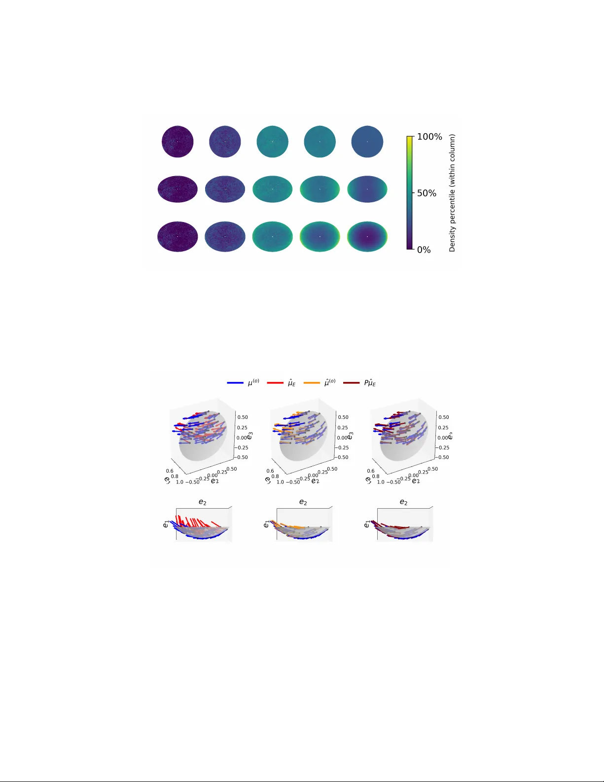
FUNCTIONAL ESTIMA TION OF MANIF OLD-V ALUED DIFFUSION PR OCESSES JACOB MCERLEAN AND HA U-TIENG WU Abstract. Nonstationary high-dimensional time series are increasingly en- countered in biomedical research as measurement technologies adv ance. Ow- ing to the homeostatic nature of physiological systems, such datasets are often located on, or can b e w ell appro ximated b y , a lo w-dimensional manifold. Mo d- eling such datasets b y manifold-v alued Itˆ o diﬀusion pro cesses has b een shown to pro vide v aluable insights and to guide the design of algorithms for clinical applications. In this pap er, we prop ose Nadaray a-W atson type nonparametric estimators for the drift vector ﬁeld and diﬀusion matrix of the pro cess from one tra jectory . Assuming a time-homogeneous sto c hastic diﬀerential equation on a smo oth complete manifold without b oundary , w e sho w that as the sam- pling in terv al and k ernel bandwidth v anish with increasing tra jectory length, recurrence of the pro cess yields asymptotic consistency and normality of the drift and diﬀusion estimators, as well as the asso ciated o ccupation density . Analysis of the diﬀusion estimator further pro duces a tangent space estima- tor for dep endent data, whic h has its own interest and is essential for drift estimation. Numerical experiments across a range of manifold conﬁgurations support the theoretical results. 1. Introduction High-dimensional time series data ha v e b ecome increasingly p erv asive across a range of quan titativ e disciplines, including but not exclusively economics, ﬁnance, geoscience, and medicine [ 11 ]. In such settings, multiple interrelated v ariables are recorded sim ultaneously o v er time, often at high sampling frequencies and ov er long horizons, resulting in complex, high-dimensional temp oral datasets. A cen tral in- feren tial ob jectiv e is to c haracterize and quantify the underlying system dynamics, either for scien tiﬁc understanding, real-time monitoring and control, or impro v ed prediction. This requires the developmen t of statistical metho ds capable of ade- quately capturing both temp oral dep endence and cross-sectional in teractions in the data. A motiv ating example from biomedicine is the repurp osing of underutilized in- traop erativ e signals, such as arterial bloo d pressure (ABP) [ 15 , 55 ] and photo- pleth ysmogram (PPG) [ 26 ], to predict clinical outcomes. By leveraging physiolog- ical knowledge, these signals can b e transformed into high-dimensional time series and in terpreted as sensors probing the dynamics of the cardiov ascular system. In particular, each cardiac cycle in an ABP signal can b e viewed as the system’s re- sp onse to a heartb eat stroke, analogous to the sound pro duced when a drum is struc k. This p erspective evok es the classical in v erse problem of whether one can “hear the shap e of a drum”. [ 30 ]. How ever, the cardio v ascular system is far more complex: it is adaptive rather than static, and its state ev olves con tin uously o ver time. Consequently , v ariabilit y across cardiac cycles [ 12 , 37 ], rather than any single 1 2 JACOB MCERLEAN AND HA U-TIENG WU w av eform, enco des critical information ab out physiological status. This observ a- tion motiv ates representing ABP as a sequence of functions, each corresp onding to a cardiac cycle, thereby forming a high-dimensional time series that captures tem- p oral evolution. Despite this v ariability , homeostatic regulation [ 41 ] ensures that these dynamics are not arbitrary but constrained by some underlying ph ysiological principles. These considerations naturally motiv ate a geometric p ersp ective for mo deling suc h data. High-dimensional biomedical time series are t ypically nonstationary and arise from deterministic dynamics mo dulated by stochastic perturbations. The underlying dynamics often evolv e on a low-dimensional, nonlinear manifold that is not directly observ able. Empirically , these tra jectories exhibit diﬀusion-like b ehav- ior ov er time, echoing reactiondiﬀusion mo dels [ 33 ] used in cardiac electrophysiol- ogy and sto chastic descriptions of heart rate v ariability [ 53 ]. While the underlying ph ysiological mechanisms are complex, only partially accessible, and usually qual- itativ e, we adopt a phenomenolo gic al approach and mo del the data as ev olving on a manifold endow ed with a diﬀusion pro cess. This approach provides a princi- pled framework for capturing intrinsic structure and enables the developmen t of algorithms for quantifying the evolving physiological dynamics. T o capture the ab ov e mentioned characteristics, we mo del a high-dimensional time series X := { x k } n k =1 ⊂ R p , where x k is sampled at time t k , using a sto chastic diﬀeren tial equation (SDE). Let ( M , g ) b e a d -dimensional Riemannian manifold isometrically em b edded in R p through ι with d ≤ p . Adapting Einstein summation con ven tion, consider an Itˆ o semimartingale X t satisfying the time-homo gene ous SDE in the Itˆ o diﬀeren tial form: (1) dX t = ν ( X t ) dt + σ α ( X t ) ◦ dW α t = µ ( X t ) dt + σ α ( X t ) dW α t ∈ M , where ν ∈ Γ ∞ ( T M ) and µ ∈ Γ ∞ ( T M ) denote the drift in the Stratonovic h and Itˆ o form, resp ectiv ely , σ α ∈ Γ ∞ ( T M ), α = 1 , . . . , r , r ∈ N , denote the diﬀusion vector ﬁelds, ◦ indicates the Stratonovic h sto chastic integral, and W t is standard r -dim Bro wnian motion. W e mo del X as discrete samples x k = ι ( X t k ) ∈ R p at t k = k ∆. Here, M reﬂects the geometric structure that constrains X t . Although the mo del pro vides a structured represen tation of the underlying sys- tem, in practice neither the parameters of the SDE nor the parametrization of the manifold M are known. Instead, we only ha v e access to the observed time series data X . This challenge has b een widely studied in the literature, though often considering M = R p ; that is, without incorp orating a nonlinear manifold in the mo del. The univ ariate case, M = R 1 , is b y now relatively well-understoo d; w e refer the reader to [ 2 , 10 ] and references therein for a broad, though not ex- haustiv e, ov erview. In the multiv ariate setting, M = R p , substan tial progress has b een made from v arious persp ectives, addressing a wide range of related challenges; non-exhaustiv e examples include nonparametric kernel-based drift and diﬀusion es- timators [ 8 , 14 , 21 ], direct cov ariance approach [ 25 ], maximal lik eliho o d approach [ 1 ], sparsit y approach [ 9 ], Malliavian-F ourier approach [ 5 , 38 ], principal comp onent analysis approach [ 4 , 13 , 16 ], sp ectral approach [ 18 , 22 ], multiscale structure based estimators [ 18 , 43 ], Gaussian pro cess approach [ 19 ], parametric approac h [ 48 ], etc. Among the challenges p osed b y this framework, in this paper we fo cus on esti- mating the drift and diﬀusion from X under the manifold mo del ( 1 ). Estimation of the o ccupation densities and tangent spaces arises as a byproduct. Our pri- mary motiv ation is [ 8 ] and [ 34 ] (in the con tinuous-time setting), which fo cuses 3 on M = R p . There, Nadara ya-W atson-type nonparametric estimators for drift and diﬀusion are prop osed, and their asymptotic prop erties are established us- ing Harris recurrence structure. T o recall the intuition b ehind the kernel regres- sion approach in [ 8 ], note that the increments 1 ∆ ( x k +1 − x k ) and outer pro ducts 1 ∆ ( x k +1 − x k )( x k +1 − x k ) ⊤ act as noisy one-step estimators of the drift ι ∗ µ ( x k ) and diﬀusion matrix P r l =1 ι ∗ σ l ( x k )[ ι ∗ σ l ( x k )] ⊤ . Individually , these quantities are highly v ariable. Kernel regression stabilizes them by aggregating lo cal estimators, assigning larger w eights to observ ations near a target p oint x via a kernel function applied to a distance scaled b y bandwidth h . The resulting weigh ted av erages yield consisten t estimators of the drift and diﬀusion. Our main con tribution is multifold, circling around generalization of the k ernel regression to the manifold setup with dep endent dataset and establishing theoreti- cal guaran tees. First, although one might attempt to directly apply the Euclidean estimator of [ 8 ], arguing that manifolds are lo cally w ell approximated by aﬃne subspaces, this in tuition fails. Even under contin uous observ ation, curv ature gen- erates a leading bias term in the Euclidean drift estimation. Sp eciﬁcally , with Itˆ o’s form ula, the Euclidean-em b edded pro cess Z t := ι ( X t ) satisﬁes d Z t =  ι ∗ ν + 1 2 D ι ∗ σ α ( ι ∗ σ α )  ( Z t ) dt + ι ∗ σ α ( Z t ) dW α t , (2) where ι ∗ ν + 1 2 D ι ∗ σ α ( ι ∗ σ α )  = ι ∗ µ = ι ∗ ν + ι ∗ | x ∇ σ α σ α and D ι ∗ σ α ( ι ∗ σ α ) is the cov ari- an t deriv ativ e of the vector ﬁeld ι ∗ σ α along itself in R p satisfying D ι ∗ σ α ( ι ∗ σ α ) = ι ∗ | x ∇ σ α σ α + I I x ( σ α , σ α ). This computation shows that if w e estimate the drift term using the Euclidean estimator, the normal comp onen t, I I x ( σ α , σ α ), biases the estimator. See Section S.1.4 for more details. Therefore, the k ernel regression pro- cedure must b e carefully designed. By contrast, curv ature do es not asymptotically aﬀect diﬀusion estimation, and the diﬀusion matrix spans the tangent space under mild assumptions. This insigh t motiv ates our construction: we ﬁrst estimate the tangen t space using the diﬀusion estimator, and then recov er the drift using the estimated tangen t structure. The resulting tangen t space estimator, deriv ed from dep enden t data, app ears to b e new in the manifold learning literature and is of indep enden t interest. Second, the sampling scheme p oses substantial challenges. Kernel regression requires suﬃciently dense lo cal sampling. In contrast to the i.i.d. framew ork commonly assumed in manifold learning [ 47 , 50 , 56 ], our data consist of a single realization of the SDE, and its empirical distribution does not automatically pro vide uniform lo cal cov erage. T o address this issue, we exploit Harris recurrence on manifolds, whic h guarantees the existence of an inv arian t measure serving as a surrogate sampling density . T o analyze the prop osed estimators, w e need a gener- alized Nummelin splitting sc heme for Harris recurrent processes, which ma y or may not hav e life cycles [ 34 ]. Com bined with the Darling-Kac result that quantiﬁes how the time X t sp ends in a region scales ov er long perio ds, w e conv ert additive func- tionals asso ciated with the estimators into in tegrals on the manifold with resp ect to X t ’s in v arian t measure. Under suitable conditions on bandwidth and sampling rates, together with careful analysis of the resulting Gaussian mixtures, we estab- lish a cen tral limit theorem for all prop osed estimators as the observ ation horizon tends to inﬁnity . This pap er is organized as follows. Section 2 presen ts the mathematical model. Section 3 details the prop osed algorithm. Theoretical results are pro vided in Sec- tion 4 , follow ed b y n umerical simulations in Section 5 . Section 6 discusses the 4 JACOB MCERLEAN AND HA U-TIENG WU ﬁndings and outlines future researc h directions. All pro ofs and tec hnical details are giv en in the App endix. W e adapt the following notation in what follows. d − − → and p − − → stand for con v ergence in distribution and con vergence in probability . F or t wo sequences of random v ariables, A n = o p ( B n ) means A n /B n p − − → 0 and A n = O p ( B n ) means A n /B n is sto c hastically b ounded as n → ∞ . The sup erscript ⊤ means ma- trix transp ose. The symbol ⊗ denotes the Kronec ker pro duct and 1 A denotes the indicator function of the set A . Other commonly used sym b ols are listed in T able S.5 . 2. Ma thema tical Model W e now present our manifold-v alued diﬀusion mo del ( 1 ) for high-dimensional time series data, viewed as observ ations ov er a ﬁnite time p erio d from a sto c hastic dynamical system. Sp eciﬁcally , we mo del the data as samples from a solution to an SDE evolving as a diﬀusion pro cess on a manifold. Assumption 1. Let ( M , g ) b e a d -dimensional, complete, connected, smo oth Rie- mannian manifold without b oundary , isometrically embedded into R p via an em- b edding ι . When the manifold is non-compact, assume the Ricci curv ature is low er b ounded; that is, Ric ≥ K g for some K ∈ R , and inj x ≥ δ > 0, where inj x is the injectivit y radius of x , for all x ∈ M . The Ricci curv ature and injectivit y assumptions hold automatically when M is compact. In the noncompact case, the lo w er b ound assumption on Ricci curv ature helps control the diﬀusion kernel behavior, and the uniform p ositiv e low er b ound assumption on the injectivity radius is imposed to preclude lo cal geometric collapse so that the v olume doubling prop erty holds. Let d g ( x, y ) denote the geo desic dis- tance b et w een x, y ∈ M and dV g denote the Riemannian volume measure. Denote b y B b ( M ), C ( M ), C 0 ( M ), and C ∞ c ( M ) the spaces of bounded measurable functions on M , contin uous functions on M , contin uous functions v anishing at inﬁnit y , and smo oth functions with compact supp ort, resp ectiv ely . Let Γ( T M ) and Γ k ( T M ), k ∈ N ∪ {∞} , denote the space of con tin uous and C k v ector ﬁelds on M . When M is noncompact, denote c M := M ∪ { ∂ M } to b e the one-p oint compactiﬁcation of M ; otherwise c M := M . Denote B ( M ) to b e the Borel σ -algebra on c M . F or a sequence x n ∈ M , w e know x n → ∂ M if and only if ∥ x n ∥ R q → ∞ [ 28 ]. Denote W r 0 := { ω ∈ C ([0 , ∞ ) , R r ) } and {F t } t> 0 its top ological σ -ﬁeld generated by Borel cylinders. Consider the probability space (Ω , F , P ) and a r -dimensional standard Bro wnian motion W s = [ W 1 s , . . . , W r s ] ⊤ with the initial distribution µ 0 . W e then ha ve a ﬁltrated probabilit y space (Ω , F ∗ , P ), where F ∗ := {F t | t ≥ 0 } is a right con tinuous ﬁltration so that F := lim t →∞ F t and F t = ∩ ϵ> 0 σ { W u | u ≤ t + ϵ } . Clearly , W t is adapted to F ∗ . Let W ( M ) := { w ∈ C ([0 , ∞ ) , c M ) | w (0) ∈ M , and if w ( t ) = ∂ M then w ( t ′ ) = ∂ M for all t ′ ≥ t } , and B t ( W ( M )) b e the topological σ -ﬁeld generated by Borel cylinders. The explosion time is deﬁned on W ( M ) by e ( w ) := inf { t | w ( t ) = ∂ M } ; that is, ∂ M is the “trap” of w . When M is compact, e = ∞ [ 49 ]. 2.1. Quic k review of SDE on manifold and assumptions. Adapt notation from ( 1 ). It is well-kno wn [ 28 , Prop osition 1.2.9] that there exists a unique strong solution, which is an R p -v alued adapted semi-martingale X t supp orted on M ⊂ R p , 5 up to its explosion time e ( X ), to a time-homogeneous SDE on manifold in the Stratono vich form: X t = X 0 + Z t 0 ν ( X s ) ds + Z t 0 σ α ( X s ) ◦ dW α s (3) where we use Einstein summation conv ention, r ∈ N , W t is the standard Brownian motion with µ 0 = δ 0 , the initial v alue X 0 ∈ M follows the distribution λ supp orted on M and is indep enden t of W t , ◦ denotes the Stratono vic h sto chastic in tegral (e.g. [ 28 , e.g., 1.1.13]), and ν , σ 1 , · · · , σ r ∈ Γ ∞ ( T M ). Recall that a strong solution to ( 3 ) up to a stopping time τ is an F ∗ -adapted random pro cess X t ∈ W ( M ) deﬁned on Ω such that for any f ∈ C ∞ ( M ) [ 28 , Deﬁnition 1.2.3], f ( X t ) = f ( X 0 ) + Z t 0 ( ν f )( X s ) ds + Z t 0 ( σ α f )( X s ) ◦ dW α s , 0 ≤ t < τ . (4) The SDE ( 3 ) is o ften written in Itˆ o diﬀerential form as that in ( 1 ). W e presen t the Stratono vich form of the integral here b ecause it respects the nonlinear geometry; that is, the Stratonovic h SDE is intrinsic to the manifold and its driving vector ﬁelds transform naturally under diﬀeomorphisms via push-forward [ 28 , Prop. 1.2.4]. Let µ X denote the probability law on W ( M ) of the solution X t to ( 3 ) and { P t } t ≥ 0 denote the asso ciated transition semigroup. Recall that for S ∈ B ( M ) and λ = δ x , where x ∈ M , for t ≥ 0, P t ( x, S ) := µ X { w ∈ W ( M ) | w ( t ) ∈ S } and P t f ( x ) := E x f ( X t ) = R W ( M ) f ( ω t ) dµ Y ( ω ), where f ∈ B b ( M ) and E x is the exp ectation asso ciated with P x . { P t } of the solution to ( 3 ) is a strong Marko v pro cess [ 20 , IX. § 3- § 5]. With a co ordinate system o ver a neigh b orhoo d U ⊂ M of x ∈ M , lo cally there is a symmetric and non-negative deﬁnite matrix-v alued function, π ( x ) := ( π ij ( x )) ∈ R d × d , where π ij ( x ) = X α σ i α ( x ) σ j α ( x ) . W e call π the diﬀusion matrix . X t is a diﬀusion pro cess whose inﬁnitesimal gener- ator L satisﬁes Lf ( x ) := lim t → 0 E x [ f ( X t )] − f ( x ) t = 1 2 r X α =1 σ α ( σ α f )( x ) + µf ( x ) , where f ∈ C ∞ c ( M ); that is, X t is a L -diﬀusion process [ 28 , Section 1.3]. In lo cal co ordinates, the generator admits the representation Lf ( x ) = 1 2 π ij ( x ) ∂ 2 f ∂ x i ∂ x j ( x ) + b i ( x ) ∂ f ∂ x i ( x ) , where b i := µ i + P α σ k α ∂ k σ i α . The additional P α σ k α ∂ k σ i α in b i arises from the con version b et w een the Itˆ o form and Stratonovic h form ulations. Harris recurrence is the key to ol for our algorithm analysis. Recall that [ 27 , Deﬁnition 1.1] X = ( X t ) t ≥ 0 with X 0 = x ∈ M a.s. is called Harris r e curr ent if there exists a non-trivial σ -ﬁnite measure η on ( M , B ( M )) so that for any A ∈ B ( M ) so that η ( A ) > 0, we ha v e P x ( R ∞ 0 1 A ( X t ) dt = ∞ ) = 1. It is well kno wn that a Harris recurrent pro cess implies the existence of a unique inv ariant measure ϕ X of { P t } , up to a constant multiple [ 27 , Theorem 1.2]. When ϕ X ( M ) = ∞ , we call X t nul l Harris r e curr ent . When ϕ X ( M ) < ∞ , we call X t p ositive Harris r e curr ent . Geometrically , the pro cess X t is Harris recurrent if, for every measurable subset of 6 JACOB MCERLEAN AND HA U-TIENG WU the manifold with p ositiv e v olume, the pro cess almost surely visits that set inﬁnitely often (in time). F or more details on Harris recurrence, w e refer readers to [ 27 ]. W e imp ose the follo wing assumption. Assumption 2. Assume the initial measure of X t , λ , is compactly supp orted on C ⊂ M with dV g ( C ) > 0 and a b ounded density function, and the sp ectrum of π ( x ) is uniformly b ounded from ab o ve and a w ay from 0; that is, L is uniformly elliptic. When the manifold is non-compact, we imp ose further assumptions. (1) (conserv ation) The explosion time is inﬁnite; that is, e ( Y ) = ∞ . (2) ( C 0 -prop ert y) { P t } is strong F eller. (3) (diﬀusion k ernel) The diﬀusion k ernel p t ( x, y ) on (0 , ∞ ) × M × M asso ciated with the transition semi-group is smo oth and strictly p ositiv e. (4) (Harris recurrence) X t is Harris recurrent with an inv arian t measure ϕ X . Note that in [ 8 ], rather than uniform ellipticit y , the H¨ ormander c ondition [ 49 , Chapter 7] is imp osed. Instead, we adopt uniform ellipticity since we need non- degenerate diﬀusion in order to design our drift estimator. The compact supp ort assumption on the initial measure is motiv ated b y biomedical applications, where it reﬂects the relatively homogeneous initial state of the dynamics. R emark 1 . Note that not ev ery choice of r is suitable for modeling and analyzing high-dimensional time series data if we need a non-de gener ate diﬀusion , which is essen tial for reco vering the drift term. Recall that the well-kno wn Hairy Ball theorem prohibits the existence of a smo oth, non-v anishing vector ﬁeld on S 2 . This top ological constrain t guarantees that c ho osing r = 2 cannot yield a non-degenerate diﬀusion on S 2 . Therefore, depending on the manifold, we may need r > d . F rom a statistical p ersp ective, taking r > d may seem to in tro duce iden tiﬁabilit y issues. In particular, it is poss ible to ﬁnd r , s ≥ d with r  = s suc h that the diﬀusion terms P r α =1 σ α ( X t ) ◦ dW α t and P s β =1 ˜ σ β ( X t ) ◦ d ˜ W β t ha ve the same law on M for some ˜ σ β and ˜ W β t , β = 1 , . . . , s , that is indepe nden t of W t . This is how ever not a big trouble in our analysis since our goal is estimating the diﬀusion matrix, not recov ering eac h σ α . Assumption 2 (1) is necessary for our analysis to b e asymptotic. Assumption 2 (2)-(4) are needed for the construction of a recurrent atom [ 27 , Deﬁnition 1.9.A] for the Nummelin-lik e splitting argumen t via an embedding tec hnique used in the analysis. Note that not all Harris recurrent pro cesses hav e a recurrent atom. The Harris recurrence assumption eﬀectively amounts to requiring suﬃcien tly dense sampling lo cally on the manifold ov er ﬁnite recording time, analogous to the “low er b ounded densit y assumption” commonly imp osed in the analysis of manifold learn- ing algorithms. See [ 27 , Chapter 1] for a summary of Harris recurrence. When M is compact, Assumption 2 (1)-(4) hold automatically . Sp eciﬁcally , the existence of smo oth kernel functions p t ( x, y ) on (0 , ∞ ) × M × M is ensured b y the H¨ ormander theorem, and p t ( x, y ) has Gaussian upp er and low er b ounds [ 49 , Theorem 6.4.1], which leads to Assumption 2 (3). Moreov er, { P t } is strong F eller [ 20 , VI I I. § 6] and X t is p ositiv e Harris recurren t [ 39 ]. When M is non-compact, v arious suﬃcien t conditions ensure Assumption 2 (1)-(4). T o av oid distraction, w e p ostpone these details to Section S.1.5 . W e shall mention that a non-compact manifold is necessary to host an Itˆ o diﬀusion with null Harris recurrence. As our primary focus is on estimating dynamics and quantifying the asymptotic b eha vior of 7 the estimators, in the non-compact case w e are conten t to work under Assumption 2 (1)-(4) in this pap er. 2.2. Manifold-v alued diﬀusion mo del and sampling for the high-dimensional time series. W e now detail the prop osed manifold-v alued diﬀusion mo del for the high-dimensional time series. W e start with a deﬁnition and some nominations. Deﬁnition 1 (Manifold-v alued diﬀusion model) . Supp ose Assumption 1 for a man- ifold M holds. W e call X t on M satisfying Assumption 2 a manifold-value d diﬀusion mo del . The high-dimensional time series X = { x k } n k =1 ⊂ R p is mo deled as the discretiza- tion of a realization of the solution ι ( X t ) on the interv al [0 , T ] at uniform times; that is, x k = ι ( X k ∆ ), where ∆ > 0 denotes the sampling interv al, k = 1 , . . . , n , n = ⌊ T / ∆ ⌋ , and ⌊·⌋ is the ﬂo or op erator. 3. Proposed algorithm Under the manifold-v alued diﬀusion mo del, w e dev elop a class of manifold- adaptiv e, Nadaray a-W atson type kernel estimators to recov er the inv ariant mea- sure ϕ X , or the o ccupation density of X t , and “observed” drift v ector and diﬀusion matrix, denoted as µ ( o ) := ι ∗ µ ∈ R p and π ( o ) := r X l =1 ( ι ∗ σ l )( ι ∗ σ l ) ⊤ ∈ R p × p , (5) from the high-dimensional time series X := { x k } n k =1 . The idea is straigh tforw ard: w e ﬁrst obtain noisy preliminary estimates of the drift and diﬀusion from pro- cess incremen ts, then av erage them using a nonparametric kernel. This “plug-in” approac h exploits v ariance reduction through a v eraging, yielding more stable and accurate estimates. In all cases, its success hinges on establishing a meaningful quan titative relationship b et w een successive observ ations x k +1 and x k b y taking care of the curv ature. In practice, the geo desic distance and tangent space of M are not av ailable and m ust b e estimated from the data. F or each state x ∈ M , prepare an appropriate “distance-lik e” function D x : M → R + deﬁned b y (6) D x ( x ′ ) := ∥ ι ( x ′ ) − ι ( x ) ∥ R p , where x ′ ∈ M , which accurately estimates the geodesic distance b etw een x and x ′ on M when they are suﬃciently close. Cho ose a kernel K : R + → R , which is smo oth and compactly supp orted. Deﬁne ˆ L ( o ) ( x ) := ∆ h d n − 1 X k =0 K  D x ( X k ∆ ) h  , whic h estimates the inv ariant measure ϕ X at x . With the chosen D x , estimate the diﬀusion matrix at x ∈ M from X by ˆ π ( o ) ( x ) = 1 ∆ P n − 1 k =0 K  D x ( x k ) h  ( x k +1 − x k )( x k +1 − x k ) ⊤ P n − 1 k =0 K  D x ( x k ) h  ∈ R p × p . (7) Note that the denominator is h d ∆ ˆ L ( o ) ( x ). 8 JACOB MCERLEAN AND HA U-TIENG WU T o estimate the drift term, we need to estimate the tangent space and a pro jec- tion onto ι ∗ T x M , denoted as ˆ P x . Denote the eigenv alue decomp osition of ˆ π ( o ) ( x ) as ˆ U x ˆ Σ x ˆ U ⊤ x , where the eigenv alues are ordered decreasingly and deﬁne (8) ˆ P x := ˆ U d ˆ U ⊤ d , where ˆ U d ∈ R p × d is formed from the ﬁrst d columns of ˆ U x . Clearly , ˆ U ⊤ d ˆ U d = I d × d b y construction. As w e show b elow, the column space of ˆ U d pro vides a go o d appro ximation of the embedded tangen t space ι ∗ T x M . With the chosen pro jection matrix ˆ P x , estimate the drift term by ˆ µ ( o ) ( x ) = ˆ P x ˆ µ E ( x ) ∈ R p , (9) where ˆ µ E ( x ) := 1 ∆ P n − 1 k =0 K  D x ( x k ) h  ( x k +1 − x k ) P n − 1 k =0 K  D x ( x k ) h  ∈ R p . (10) When M = R p , our problem re duces to that studied in [ 8 ]. Indeed, choosing ˆ P x = I p × p mak es the estimators in ( 7 ) and ( 9 ) coincide with those of [ 8 ]. In the manifold setting, particularly when d < p and M is nonlinear, the situation diﬀers. Although the diﬀusion pro cess can be embedded in Euclidean space, the estimator of [ 8 ], denoted ˆ µ E , targets the drift of the embedded pro cess Z t rather than that of X t ; see ( 2 ). A simple illustration is the curve M = { ( x, y ) : y = x 2 } . Driftless Brownian motion on R lifts naturally to M , yet a naive drift estimate at (0 , 0) acquires a positive vertical comp onent normal to M , ev en when geo desic distances on M are used. T o correct curv ature-induced bias, a pro jection matrix ˆ P x is necessary . R emark 2 . Recall that when x and x ′ are suﬃciently close, the Euclidean distance ∥ ι ( x ′ ) − ι ( x ) ∥ R p pro vides a go o d approximation to the geo desic distance [ 36 ]; that is, when x ′ = exp x ( tθ ), ∥ θ ∥ = 1, and t suﬃciently small, w e ha ve ∥ ι ( x ) − ι ( x ′ ) ∥ R q = t + 1 6 t 3 ι ∗ θ ⊤ ∇ θ I I x ( θ , θ ) + O ( t 4 ) , where I I x is the second fundamen tal form at x . More accurate appro ximations can b e obtained through higher-order corrections inv olving estimating the second fundamen tal form [ 36 ], and in some settings geo desic information ma y even b e a v ailable. How ev er, the main diﬃcult y arises not from estimating geodesic distances but from analyzing the increment x k +1 − x k . In general, x k +1 − x k do es not lie in ι ∗ T x M and contains a normal comp onen t, whic h is the primary source of bias. F or this reason, we do not pursue higher-order lo cal appro ximations of the geo desic distance here. 4. Asymptotic Anal ysis In this section, w e study the asymptotic behavior of the estimators introduced in Section 3 . W e b egin with in tuition and relev ant existing results b efore presen ting main results. In tuitively , since X t is contin uous, our prop osed estimators can b e viewed as Riemann sum approximations of their target quantities. T o b e more sp eciﬁc, b y 9 Itˆ o’s formula, we ha ve x k +1 − x k = ι ( X ( k +1)∆ ) − ι ( X k ∆ ) = Z ( k +1)∆ k ∆ µι ( X s ) ds + Z ( k +1)∆ k ∆ σ α ιdW α s , and hence the numerator of ˆ µ E ( x ) becomes 1 h d n − 1 X k =0 K  D x ( x k ) h  Z ( k +1)∆ k ∆ µι ( X s ) ds + Z ( k +1)∆ k ∆ σ α ιdW α s ! . By appro ximating R ( k +1)∆ k ∆ µι ( X s ) ds b y ∆ µι ( X k ∆ ), w e ha v e: ˆ µ ( o ) ( x ) ≈ P x  ∆ h d P n − 1 k =0 K  D x ( x k ) h  µι ( X k ∆ ) ∆ h d P n − 1 k =0 K  D x ( x k ) h  + 1 h d P n − 1 k =0 K  D x ( x k ) h  R ( k +1)∆ k ∆ σ α ιdW α s ∆ h d P n − 1 k =0 K  D x ( x k ) h   , where the summation is the Riemann sum approximation; that is, ∆ h d P n − 1 k =0 K  D x ( x k ) h  µι ( X k ∆ ) ∆ h d P n − 1 k =0 K  D x ( x k ) h  ≈ 1 h d R T 0 K  D x ( X s ) h  µι ( X s ) ds 1 h d R T 0 K  D x ( X s ) h  ds . (11) The ﬁrst term in ( 11 ) is the ratio of tw o integrations inv olving X t . Recall that for b ounded measurable f ≥ 0, an R + ∪ {∞} v alued, F t -adapted pro cess A t := R t 0 f ( X s ) ds , t ≥ 0, with A 0 = 0, is called an additive functional . See Section S.1.1 for more details. By deﬁnition, the denominator 1 h d R T 0 K  D x ( X s ) h  ds is an additiv e functional, and the n umerator can b e handled similarly using addi- tiv e functional prop erties after prop er manipulations. In the pro of, we quan- tify these approximations and show that this term, combined with P x appro xi- mates the desired drift. The second term in ( 11 ) in volv es sto chastic integration, 1 h d P n − 1 k =0 K  D x ( x k ) h  R ( k +1)∆ k ∆ σ α ιdW α s , which we c on trol via controlling its qua- dratic v ariation using its martingale property . In the end, we show that it con v erges to a normal distribution. Since all proposed estimators share a similar structure, while some might b e more complicated than others, the analysis reduces to con- trolling the Riemann sum approximation when ∆ → 0, quantifying the b ehavior of the integrals when h → 0 and T → ∞ , and analyzing the asymptotics of the sto c hastic integral terms. The ratio of t w o integrations inv olving X t reminds us of the ratio-limit theorem. Theorem 4.1 (Ratio Limit Theorem) . [ 27 , The or em 1.7] Supp ose Assumptions 1 and 2 hold. F or any Bor el-me asur able, p ositive, and ϕ X -inte gr able f , g : M → R such that 0 < ⟨ ϕ X , g ⟩ M := R M g ( x ) ϕ X ( x ) < ∞ , we have P x lim T →∞ R T 0 f ( X s ) ds R T 0 g ( X s ) ds = ⟨ ϕ X , f ⟩ M ⟨ ϕ X , g ⟩ M ! = 1 (12) for al l x ∈ M . Mor e over, lim T →∞ E x R T 0 f ( X s ) ds E x R T 0 g ( X s ) ds = ⟨ ϕ X , f ⟩ M ⟨ ϕ X , g ⟩ M (13) ϕ X -a.s., wher e the exc eptional set dep ends on f and g . 10 JACOB MCERLEAN AND HA U-TIENG WU This theorem shows that, in the long-time limit, an additiv e functional b eha v es lik e an integral ov er the manifold, and it links our analysis with that in mani- fold learning via ( 11 ). In other words, the eﬀect of the initial condition is eﬀec- tiv ely “washed out” asymptotically , linking the result to the ergodic theorem, with R T 0 g ( X s ) ds acting as a random clo c k counting eﬀective time. See Section S.1.3 for further details. T o quantify the asymptotic b ehavior of additive functionals, we need to know ho w often the system X t returns to a given state and ho w the time sp en t in a region scales ov er long p erio ds. When X t is Harris recurren t, these quan tities follo w a w ell- deﬁned probabilistic pattern that typically resem bles a stable distribution rather than the usual b ell-curve b ehavior. This fact is quantiﬁed in the following general Darling-Kac theorem. T o state this theorem, we need the notion of a function that, while not necessarily b ounded, b ehav es asymptotically like a constan t. Deﬁnition 2. Let ℓ : R + → R + . W e say that ℓ is r e gularly varying at inﬁnity with index α ∈ R if for all ζ > 0, lim x →∞ ℓ ( ζ x ) ℓ ( x ) = ζ α . If α = 0, ℓ ( x ) is called slow ly varying at inﬁnity . W e similarly say that ℓ is r e gularly varying at zer o with index α if for all ζ > 0, lim x → 0 ℓ ( ζ x ) ℓ ( x ) = ζ α . Denote D ( R + , R ) to b e the Skorohod space with Borel σ -algebra and canonical ﬁltration. Note that the classical Darling-Kac theorem is the necessary direction of the follo wing theorem, so we call it the general Darling-Kac theorem. Theorem 4.2 (General Darling-Kac Theorem) . [ 27 , The or em 3.15] Supp ose As- sumptions 1 and 2 hold. (a) The fol lowing two statements ar e e quivalent. (1) F or every non-ne gative Bor el-me asur able function g with 0 < ⟨ ϕ X , g ⟩ M < ∞ , one has r e gular variation at 0 of r esolvants in X t : ( R 1 /T g )( x ) := E x  Z ∞ 0 exp  − t T  g ( X t ) dt  ∼ ⟨ ϕ X , g ⟩ M Υ( T ) (14) as T → ∞ for p X -almost al l x ∈ M (the exc eptional set dep ends on f ), wher e Υ( T ) := U ( T ) T α , α ∈ (0 , 1] , and U : R + → R + is slow ly varying at inﬁnity. (2) F or any additive functional A t = R t 0 f ( X s ) ds of X t with 0 < E ϕ X ( A 1 ) < ∞ , one has we ak c onver genc e ( A sT ) s ≥ 0 Υ( T ) d − − → E ϕ X ( A 1 ) g α ( s ) in D ( R + , R ) as T → ∞ under P x for al l x ∈ M , wher e g α is the Mittag- L eﬄer pr o c ess of index α . (b) The c ases in (a) ar e the only ones that the we ak c onver genc e of ( A sT ) s ≥ 0 υ ( T ) to a c ontinuous nonde cr e asing limit pr o c ess ϖ so that ϖ 0 = 0 and the law of ϖ 1 is not de gener ate at 0 , is available for some norming function υ . See Section S.1.2 for a quic k review of Mittag-Leﬄer pro cess. Call Υ : R + → R + the sc aling factor of X t . When the manifold is compact, X t is p ositive Harris recurren t and w e ha v e Υ( T ) = T , or α = 1, and U ( T ) = 1. 11 4.1. F urther mo del assumptions. Denote the densities of X t and X s and the corresp onding joint density as ˜ p t ( · ), ˜ p s ( · ), and ˜ p s,t ( · , · ) resp ectiv ely , and denote (15) ˜ g s,t ( a, b ) = ˜ p s,t ( a, b ) − ˜ p s ( a ) ˜ p t ( b ) , where a, b ∈ M , which quan tiﬁes the lev el of path-dep endence of the pro cess X t . W e mak e the following assumption ab out Υ’s b ehavior near 0, which allows us to apply Theorem 4.2 , and the regularity of the path-dep endence of the pro cess via the scaling factor Υ. Assumption 3. The scaling factor Υ of X t is regularly v arying at 0 with index α ∈ (0 , 1]. Moreo ver, lim T →∞ Υ( T ) − 1 Z Z [0 ,T ] 2 ∥ ˜ g s,t ∥ r ds dt < ∞ for some r ∈ [1 , ∞ ]. In other words, the ﬁrst part of Assumption ( 3 ) says that Theorem 4.2 (a)(1) holds. W e imp ose the follo wing assumption for ϕ X , whic h allows us to carry out asymptotic analysis on M . Assumption 4. The inv ariant measure ϕ X asso ciated with X t is absolutely con- tin uous asso ciated with the Riemannian measure of the manifold M and admits a strictly-p ositiv e density function p X ∈ C 3 ( M ) so that ϕ X ( dx ) = p X ( x ) dV g ( x ) by Radon-Nik o dym theorem. 4.2. Sampling and algorithm assumptions. Our ﬁnal set of assumptions con- cerns the data sampling scheme and algorithm. Regarding the kernel function K , w e mak e the follo wing assumption. Assumption 5. The kernel function K ∈ C 3 ( R ) is nonnegative and compactly supp orted on [0 , L ], where L > 0. Denote κ p,q = R R d K ( ∥ u ∥ ) p ∥ u ∥ q du , where p ∈ N and q ∈ { 0 } ∪ N , and assume κ 1 , 0 = 1. The assumption κ 1 , 0 = 1 can b e easily ac hiev ed b y a direct normalization. Fi- nally , we mak e an assumption regarding the sampling perio d ∆ and bandwidth h , whic h dep ends on the scaling factor Υ of X t . Assumption 6. Assume ∆ = ∆( T ) → 0, h = h ( T ) → 0, and Υ( T ) h 2 d/r → ∞ , where r is from Assumption 3 , as T → ∞ . This assumption pla ys a crucial role in our analysis. Letting T → ∞ allows us to lev erage the equilibrium b ehavior of the dynamics to estimate b oth drift and diﬀusion terms, while ∆ → 0 provides suﬃcien tly ﬁne temp oral resolution to capture the dynamics accurately , often referred to as inﬁl ling asymptotics. 4.3. Asymptotic result for prop osed estimators. Recall notation in Section 3 . W e start with the asymptotic behavior of ˆ L ( o ) ( x ), whic h is stated in the follo wing Theorem and its pro of is p ostp oned to Section S.3 . Theorem 4.3 (Occupation densit y estimator) . Assume Assumptions 1 - 6 hold. If ∆ h 2 = o (1) as T → ∞ , we have ˆ L ( o ) ( x ) Υ( T ) d − → g α (1) p X ( x ) and E M λ ( ˆ L ( o ) ( x )) = Θ(Υ( T )) . (16) Geometrically , ˆ L ( o ) ( x ) is an estimate of the inv ariance measure asso ciated with X t , which can b e viewed as a kernel density estimation of p X ( x ) when the samples are dependent and mo deled by a diﬀusion pro cess. 12 JACOB MCERLEAN AND HA U-TIENG WU Next, we discuss the diﬀusion estimator. T o describ e the bias of the estimator ˆ π ( o ) ( x ), deﬁne b ( o ) π ( x ) := κ 1 , 2  ∇ π ( o ) ( x ) · ∇ log p X ( x ) + 1 2 ∆ π ( o ) ( x )  . (17) W e hav e the following theorem describing the asymptotic behavior of ˆ π ( o ) ( x ). Theorem 4.4 (Diﬀusion estimator) . Supp ose Assumptions 1 - 6 hold. F urther sup- p ose that h d Υ( T ) ∆ − → ∞ , h d +4 Υ( T ) ∆ − → C for a c onstant C > 0 , and h d − 4 Υ( T )∆ − → 0 . When T → ∞ , we have s h d ˆ L ( o ) ( x ) ∆ ( ˆ π ( o ) ( x ) − π ( o ) ( x ) − h 2 b ( o ) π ( x )) d − → N  0 , 2 κ 2 , 0 π ( o ) ( x ) ⊗ π ( o ) ( x )  , (18) wher e ⊗ is the Kr one cker pr o duct. When M = R d , our framework and results reduce to those of [ 8 , Theorem 5], where the result is introduced using half-vectorization. Denote vech and vec to b e the half-vectorization and v ectorization op erators that conv ert an y symmetric matrix A ∈ R m × m in to vech ( A ) ∈ R m ( m +1) / 2 and vec ( A ) ∈ R m 2 . Denote D ∈ R m 2 × m ( m +1) 2 to be the standard duplication matrix that con v erts vech ( A ) in to vec ( A ) for any symmetric matrix A ∈ R m × m . Then, ( 18 ) can b e rewritten as s h d ˆ L ( o ) ( x ) ∆ v ech( ˆ π ( o ) ( x ) − π ( o ) ( x ) − h 2 b ( o ) π ( x )) d − → N (0 , 2 κ 2 , 0 P D  π ( o ) ( x ) ⊗ π ( o ) ( x )  P ⊤ D ) , where P D = ( D ⊤ D ) − 1 D ⊤ . In the manifold setting, the deviation of ( x i +1 − x i ) from ι ∗ T x i M comes in to pla y , whic h complicates the bias terms in ( 18 ) through curv ature eﬀects. Notably , b oth the bias and v ariance dep end on the in trinsic manifold dimension d , rather than the ambien t dimension p . R emark 3 . Note that [ 8 , Theorems 5] imp oses the conditions h d ˆ L ( o ) ( x ) ∆ p − → ∞ , h d +4 ˆ L ( o ) ( x ) ∆ p − → C , and h d − 4 ˆ L ( o ) ( x )∆ p − → 0. W e choose to replace ˆ L ( o ) ( x ) b y Υ( T ) in our assumption to av oid potential con tradiction. Indeed, if w e impose h d +4 ˆ L ( o ) ( x ) ∆ p − → C , with Theorem 4.3 that ˆ L ( o ) ( x ) Υ( T ) d − → g α (1) p X ( x ), Slutsky’s theorem and con tinuous mapping theorem give h d +4 Υ( T ) ∆ p − → C g α (1) p X ( x ) . When α ∈ (0 , 1), since h d +4 Υ( T ) ∆ is a deterministic sequence and g α (1) is a nondegenerate random v ariable, we m ust ha ve C = 0, and hence lose the control of h d +4 ˆ L ( o ) ( x ) ∆ . As discussed in [ 8 , Remark 12], it is not a problem to replace ˆ L ( o ) ( x ) by Υ( T ) in [ 8 , Theorems 5] (and [ 8 , Theorems 4] as well), which av oids the contradiction. The same comment holds for Theorem 4.6 . Estimating the drift estimator is more delicate, as it requires estimating the tangen t-space pro jection of the embedded manifold from the data. The following theorem pro vides a key result for tangent space estimation. Theorem 4.5 (T angent space estimator) . Supp ose Assumptions 1 - 6 hold. Denote P x to b e an ortho gonal pr oje ction to ι ∗ T x M . Supp ose mor e over that h d Υ( T ) − → ∞ , h d +4 Υ( T ) − → C for a c onstant C > 0 , and ∆ 2 h d − 4 Υ( T ) − → 0 . Denote the eigenvalue de c omp osition ˆ π ( o ) ( x ) = ˆ U ˆ D ˆ U ⊤ , wher e the eigenvalues ar e or der e d descr e asingly. 13 L et ˆ U d b e the p × d matrix forme d fr om the ﬁrst d c olumns of ˆ U asso ciate d with the lar gest d eigenvalues. Then, ˆ P x := ˆ U d ˆ U ⊤ d = P x + h 2 b ( t ) ( x ) , (19) wher e b ( t ) ( x ) = b ( t ) ( x )+ ϵ ( t ) ( x ) ∈ R p × p , b ( t ) ( x ) = O (1) , and ϵ ( t ) ( x ) = o p  1 √ h d +4 Υ( T )  . Note that the central limit theorem for the diﬀusion estimator dep ends on the scale q ∆ h d ˆ L ( o ) ( x ) , whereas tangent space recov ery only requires the coarser scale 1 √ h d ˆ L ( o ) ( x ) . This diﬀerence arises b ecause the latter scale is already suﬃcient for establishing the cen tral limit theorem for drift estimation. W e do not claim opti- malit y of the prop osed diﬀusion-based tangent space estimator. W e also note that sev eral metho ds for tangent space estimation hav e b een proposed in the literature (e.g., [ 47 , 50 ]), primarily based on lo cal principal comp onent analysis (PCA). In this approac h, one constructs a lo cal cov ariance matrix C x := n − 1 X k =0 K  D x ( x k ) h  ( x k − x )( x k − x ) ⊤ , and estimates ι ∗ T x M using its top d eigenv ectors. How ever, these metho ds t ypically assume i.i.d. samples from the manifold and th us do not directly apply in our setting. Additional analysis is required to understand the b ehavior of local PCA under the manifold-v alued diﬀusion mo del. T o state the asymptotic b eha vior of ˆ µ ( o ) , deﬁne the bias term: b ( o ) µ ( x ) = κ 1 , 2 P x  ∇ µ ( o ) ( x ) · ∇ log p X ( x ) + 1 2 ∆ µ ( o ) ( x )  − b ( t ) ( x ) µ ( o ) ( x ) ∈ R p , (20) where b ( t ) ( x ) is in ( 19 ). Theorem 4.6 (Drift estimator) . Supp ose Assumptions 1 - 6 hold. Supp ose mor e over that h d Υ( T ) − → ∞ , h d +4 Υ( T ) − → C for a c onstant C > 0 , and ∆ 2 h d − 4 Υ( T ) − → 0 . Supp ose P x is the ortho gonal pr oje ction to ι ∗ T x M . When T → ∞ , q h d ˆ L ( o ) ( x )( ˆ µ ( o ) ( x ) − µ ( o ) ( x ) − h 2 b ( o ) µ ( x )) d − → N ( 0 , κ 2 , 0 P x π ( o ) ( x ) P ⊤ x ) . (21) In the case where M = R d , the drift estimator reduces to that considered in [ 8 ]. Since the SDE can b e constructed via an em b edding pro cedure, it is tempting to directly apply the estimator from [ 8 ]. Ho w ev er, this naiv e approach in tro duces an additional bias of order 1 in the normal direction due to curv ature. More sp eciﬁcally , if w e omit ˆ P x and simply use ˆ µ E ( x ) ( 9 ), we hav e q h d ˆ L ( o ) ( x )( ˆ µ E ( x ) − ( µ ( o ) ( x ) + µ ( o ) η ( x )) − h 2 b ( o ) µ ( x )) d − → N (0 , κ 2 , 0 π ( o ) ( x )) , whic h diﬀers from ( 21 ) by a nontrivial term µ ( o ) η ( x ) = 1 2     P d a =1 P d b =1 ⟨ σ ( o ) a ( y ) , σ ( o ) b ( y ) ⟩ e ⊤ 1 I I y ( ∂ a , ∂ b ) . . . P d a =1 P d b =1 ⟨ σ ( o ) a ( y ) , σ ( o ) b ( y ) ⟩ e ⊤ p I I y ( ∂ a , ∂ b )     ∈ R p 14 JACOB MCERLEAN AND HA U-TIENG WU living in the normal space at x . The deviation µ ( o ) η ( x ) cannot b e eliminated even if w e can access the geo desic distance of the manifold and set D x ( x k ) = d g ( x, x k ) in ˆ µ E ( x ). See Figure 2 in the n umerical section for examples. W e emphasize a key tec hnical distinction betw een the analyses of the diﬀusion and drift estimators. F or the drift, four error terms must be con trolled in the expansion of the exp onen tial map. This arises because the drift of a diﬀusion pro cess acquires second-order contributions under a co ordinate transformation via geometry-sto c hastics relationship, which is made clear via Itˆ o’s lemma. As a result, curv ature, the second-order structure of the manifold, induces a non-negligible dis- tortion in the drift that p ersists asymptotically . Note that ev en in the Euclidean setting, the bias con tains a second-order term originating from the drift itself [ 8 , Theorem 4]. W e compare the bandwidth-sampling size pair ( h, n ) for the drift and diﬀusion estimators with the c hoices commonly used in the manifold learning literature. In manifold learning, observ ations are t ypically assumed to b e indep endent. F or p oin t wise conv ergence, the bandwidth h = h ( n ) is usually c hosen such that nh d → ∞ and h → 0 as n → ∞ . Geometrically , if the sampling density is b ounded a w a y from 0, the condition nh d → ∞ ensures that asymptotically there are inﬁnitely man y samples in a shrinking ball of radius h , pro viding suﬃcient lo cal data for estimation. While the relationship is more complicated, a parallel condition for the drift estimator is h d Υ( T ) → ∞ as T → ∞ . When X t is p ositive Harris recurrent, for example, M is compact, Υ( T ) = T . Using the sampling relation T = n ∆ with ∆ → 0 as T → ∞ , the assumption can b e rewritten as h d n ∆ → ∞ as n → ∞ . The interpretation is similar but not identical to the indep enden t-sampling case. Since ∆ → 0, the condition implies h d n → ∞ , so that asymptotically inﬁnitely man y observ ations fall in a lo cal neighborho o d. The additional factor ∆ slows the eﬀective rate and requires more observ ations when the sampling in terv al is small, reﬂecting the stronger temp oral dep endence b et ween closely spaced samples. Under the same p ositive Harris recurrent condition, the condition h d Υ( T ) ∆ → ∞ when T → ∞ for the diﬀusion estimator is equiv alent to h d n → ∞ as n → ∞ . Th us, when T and ∆ are ﬁxed across pro cedures, and hence the same sample size, ˆ π ( o ) con verges faster than ˆ µ ( o ) b y a factor of √ ∆. This theoretical ﬁnding has an in tuitive in terpretation. F rom ( 2 ), ι ( X ( k +1)∆ ) − ι ( X k ∆ ) =  ι ∗ ν + 1 2 D ι ∗ σ α ( ι ∗ σ α )  ( ι ( X k ∆ ))∆ + ι ∗ σ α ( X k ∆ ) √ ∆ Z α + o p (∆ 3 / 2 ) , where Z α ∼ N (0 , 1). In this approximation, the drift term is of order ∆, while the diﬀusion term, or noise, is of order √ ∆. When ∆ gets smaller, the signal-to- noise ratio for the drift decreases at rate √ ∆; the sto c hastic ﬂuctuations dominate the deterministic drift contribution in each incremen t, making its recov ery more diﬃcult. In contrast, ( ι ( X ( k +1)∆ ) − ι ( X k ∆ ))( ι ( X ( k +1)∆ ) − ι ( X k ∆ )) ⊤ = ( ι ∗ σ α ( X k ∆ ) Z α )( ι ∗ σ α ( X k ∆ ) Z α ) ⊤ ∆ + O p (∆ 3 / 2 ) , so the diﬀusion co eﬃcient app ears in the leading term of the increment. Conse- quen tly , the diﬀusion comp onen t is statistically easier to estimate than the drift. 15 5. Simula ted Experiments In this section, w e examine our prop osed estimators using tw o 2-dimensional manifolds, the standard 2-sphere S 2 = { x ∈ R 3 : ∥ x ∥ = 1 } ⊂ R 3 and the Klein b ottle embedded in R 4 . Throughout this section, we use a smo oth, com- pactly supp orted kernel function deﬁned by K ( s ) = exp( − (1 − ( s/ 3) 2 ) − 1 ) when s ∈ [0 , 3) and 0 otherwise. Bandwidth selection is delicate in practice, particularly when the sampling densit y is non uniform. Since developing a bandwidth selec- tion algorithm is b ey ond the scop e of this work, w e follow the empirical practice in manifold learning and select h so that the kernel is supp orted on a neighbor- ho od that is of size ∼ 1% of the total tra jectory length. The problem of iden- tifying an optimal bandwidth will b e inv estigated in future studies (see Discus- sion). The Python co de producing ﬁgures and results are av ailable in https: //github.com/jacobmcerlean/Functional- Estimation- Manifold- SDEs . 5.1. 2 -sphere. Consider M as a 2-dim ellipsoid with eccentricit y ( a, b, c ) em b edded in R 3 . T o simulate SDE tra jectories on M , consider S 2 ⊂ R 3 and diﬀeomorphism from S 2 to M via φ : ( x, y , z ) 7→ ( ax, by , cz ). Consider the SDE with the drift µ ( l ) ( x, y , z ) = ( y , − x, 0) and Riemannian Bro wnian motion on S 2 . W e simulate the pro cess using a r etr action-b ase d Euler scheme [ 45 ], which is detailed b elow. Giv en a num b er of observ ations n ∈ N , time-step size ∆, and an initial condition Y 0 = y 0 ∈ S 2 , we generate a discrete tra jectory { Y k } n k =0 on S 2 as follows. F or k = 0 , . . . , n − 1, we ﬁrst sample a random unit vector w k ∈ R 3 and an independent random χ 2 (2)-distributed radius r k . Then, we set a random tangen t v ector v k := r k  w k − w ⊤ k Y k Y k | w k − w ⊤ k Y k Y k |  ∈ T Y k S 2 . This produces an isotropic tangent incremen t consistent with Riemannian Brownian motion on S 2 . The Euler incr ement is then deﬁned by δ Y k = √ ∆ v k + ∆ µ ( Y k ) . (22) The next state of the SDE tra jectory is obtained via a retraction map given by radial pro jection; that is, Y k +1 := Y k + δ Y k ∥ Y k + δ Y k ∥ . Then iterate with k . As is sho wn in [ 45 ], this iteration approximates the in trinsic SDE on S 2 . The drift of X t = φ ( Y k ) is µ (o) ( x, y , z ) =  ay b , − bx a , 0  + P ( x,y ,z ) ( − ( x, y , z )) , where P ( x,y ,z ) w = w − ⟨ w , n ( x, y , z ) ⟩ ⟨ n ( x, y , z ) , n ( x, y , z ) ⟩ n ( x, y , z ) , n ( x, y , z ) =  x a 2 , y b 2 , z c 2  . and diﬀusion is π (o) ( x, y , z ) = D φD φ ⊤ − ( x, y , z )( x, y , z ) ⊤ , where D φ ∈ R 3 × 3 is the matrix diag( a, b, c ). No w we rep ort results on an ellipsoid M with eccentricit y ( a, b, c ) = (2 , 1 . 5 , 1), normalized b y applying a global scaling q 3 a 2 + b 2 + c 2 , and p ostp one results for other ellipsoids with eccentricities (1 , 1 , 1) and (1 . 5 , 1 , 1) with the same normalization to Section S.7 . W e start with demonstrating the rate of conv ergence of the empirical density of an SDE tra jectory to the in v arian t measure of X t . Simulate a long tra jectory of length n max = 10 8 and ∆ = 10 − 2 , for physical time T = 10 6 , on S 2 , and map this tra jectory to M . In Figure 1 , we rep ort the log-log plot of ∥ ˆ L ( o ) − ϕ X ∥ L 2 to demonstrate the rate of conv ergence of the empirical density . The decay rate of 16 JACOB MCERLEAN AND HA U-TIENG WU around n − 1 / 2 agrees with the positive Harris recurrence nature of the dynamics. F or a visualization, we plot the empirical density ˆ L ( o ) ( x ) of the tra jectory at diﬀerent lengths n i , where log 10 ( n i ) ∈ { 4 , 5 , 6 , 7 , 8 } , in Figure S.7 . Figure 1. Using the o ccupation density for tra jectory length n = 10 8 , time-step ∆ = 10 − 2 , and physical time T = 10 6 as an accurate estimate for the inv arian t densit y ϕ X , we compare the inv arian t densit y to the estimate ˆ L ( o ) based on the ﬁrst n data-p oints of the tra jectory on each observed ellipsoid to measure the conv ergence rate of the empirical density . Next, w e simulate an SDE tra jectory of length n = 10 8 , with the initial p oint sampled uniformly from N , time step ∆ = 10 − 4 , and physical time T = 10 4 . The dataset is obtained b y do wnsampling the tra jectory , k eeping ev ery 100 th observ a- tion. This preserv es the ph ysical time while reducing the sample size to n = 10 6 with uniform time step ∆ = 10 − 2 . Figure 2 illustrates ˆ µ E ( x ) and ˆ µ ( o ) ( x ) computed from the dataset on M is (2 , 1 . 5 , 1), shown on a spherical cap near (2 , 0 , 0). Additional examples with diﬀer- en t eccentricities are provided in Figures S.8 and S.9 . The curv ature-induced bias of ˆ µ E ( x ) is clearly visible in Figure 2 . F or comparison, we also plot P ˆ µ E , which is deﬁned as ( P ˆ µ E )( x ) := P x ˆ µ E ( x ), where P x is the true pro jection op erator onto ι ∗ T x M . As expected, when the tangen t space is known, P ˆ µ E visually p erforms b etter than ˆ µ ( o ) . T o quan tify these observ ations, w e sample 10 4 p oin ts uniformly on S 2 , map them to M , and ev aluate drift and diﬀusion estimation errors at these base-p oints. Due to the top ological constraints, any contin uous drift on S 2 m ust v anish somewhere. T o a void numerical instability , we stratify p oints by ∥ µ ( o ) ( x ) ∥ / ∥ µ ( o ) ∥ ∞ with threshold c = 0 . 05. F or the subset of p oin ts with {∥ µ ( o ) ( x ) ∥ / ∥ µ ( o ) ∥ ∞ > 0 . 05 } (99 . 9% out of 10 4 ), w e report: (i) relative vector error, or normalized root mean square error (NRMSE), ∥ ˆ µ − µ ( o ) ∥ ∥ µ ( o ) ∥ , where ˆ µ can b e any drift estimator, (ii) relative norm error |∥ ˆ µ ∥−∥ µ ( o ) ∥| ∥ µ ( o ) ∥ , and (iii) angle error Θ( ˆ µ, µ ( o ) ) with the unit radians. F or the remaining p oin ts, where the drift is near zero, we rep ort absolute drift errors ∥ ˆ µ − µ ( o ) ∥ only . F or diﬀusion, we rep ort the relativ e F rob enius error, or NRMSE, ∥ ˆ π − π ∥ F ∥ π ∥ F and a subspace metric based on principal angles b et ween the leading tw o-dimensional 17 eigenspaces, U 2 (resp. b U 2 ), of π (resp. ˆ π ), ∥ sin Θ 2 ∥ F , where sin Θ 2 := sin Θ( U 2 , b U 2 ), with Θ( U 2 , b U 2 ) the diagonal matrix so that the singular v alues of U ⊤ 2 b U 2 are the cosines of the diagonal matrix Θ( U 2 , b U 2 ). Note that ∥ sin Θ 2 ∥ F measures the error of tangen t space estimation. Summary statistics (means ± standard deviations) are reported in T able 1 , with the associated histograms in Figures S.10 and S.11 . Results for M with other ec- cen tricities are sho wn in T able S.3 . Consistently smaller diﬀusion errors compared to drift errors reﬂect the greater diﬃculty of drift estimation discussed after The- orem 4.6 . The drift estimators exhibit the predicted ordering: ˆ µ E has the largest error, ˆ µ ( o ) impro ves upon it, and P ˆ µ E p erforms best. This pattern holds across rel- ativ e vector, norm, and angle errors. Paired one-sided Wilco xon signed-rank tests with Bonferroni correction conﬁrm P ˆ µ E < ˆ µ ( o ) < ˆ µ E for all drift metrics (adjusted p -v alues < 10 − 5 ). Finally , a detailed study at (0 , 0 , 1) ⊤ , based on 1000 indep enden t SDE simula- tions with n = 10 6 and ∆ = 10 − 2 can b e found in Figures 3 and 4 . The approx- imately Gaussian error distributions align with the asymptotic normality result; QQ-plots are provided in Figures S.12 and S.13 . Figure 2. F rom left to right: visualizations of ˆ µ E ( x ) , ˆ µ ( o ) ( x ) , and P x ˆ µ E ( x ), where P x is the pro jection op erator on to the tan- gen t space T x M , for base-p oint samples x drawn uniformly from a spherical cap centered at (1 , 0 , 0) ⊤ and observed on an ellipsoid with eccentricit y (2 , 1 . 5 , 1), sho wn from tw o viewing angles. The ground-truth drift vector is sup erimp osed as blue arro ws. 5.2. The Klein Bottle in R 4 . Set N := [0 , 2 π ) × [0 , 2 π ). Consider the manifold M to b e the Klein b ottle K ⊂ R 4 , a compact, non-orien table, 2-dimensional smo oth manifold without b oundary , em b edded in R 4 via the smo oth map φ : ( u, v ) ∈ N → [cos( u )( a + r sin v ) , sin( u )( a + r sin v ) , r cos( u/ 2) sin v , r sin( u/ 2) sin v ] ⊤ , where 18 JACOB MCERLEAN AND HA U-TIENG WU Error type ˆ µ E ˆ µ ( o ) P x ˆ µ E ˆ π ( o ) ∥ ˆ µ ( x ) − µ ( o ) ( x ) ∥ ∥ µ ( o ) ( x ) ∥ ( ∥ µ ( o ) ( x ) ∥ ∥ µ ( o ) ∥ ∞ ≥ 0 . 05) 1 . 060 ± 0 . 566 0 . 215 ± 0 . 215 0 . 208 ± 0 . 214 — |∥ ˆ µ ( x ) ∥−∥ µ ( o ) ( x ) ∥| ∥ µ ( o ) ( x ) ∥ ( ∥ µ ( o ) ( x ) ∥ ∥ µ ( o ) ∥ ∞ ≥ 0 . 05) 0 . 474 ± 0 . 507 0 . 150 ± 0 . 169 0 . 147 ± 0 . 167 — Θ( ˆ µ ( x ) , µ ( o ) ( x )) ( ∥ µ ( o ) ( x ) ∥ ∥ µ ( o ) ∥ ∞ ≥ 0 . 05) 0 . 782 ± 0 . 190 0 . 129 ± 0 . 192 0 . 124 ± 0 . 193 — ∥ ˆ µ ( x ) − µ ( o ) ( x ) ∥ ( ∥ µ ( o ) ( x ) ∥ ∥ µ ( o ) ∥ ∞ < 0 . 05) 0 . 644 ± 0 . 013 0 . 126 ± 0 . 060 0 . 125 ± 0 . 059 — ∥ ˆ π ( x ) − π ( o ) ( x ) ∥ F / ∥ π ( x ) ∥ F — — — 0 . 038 ± 0 . 013 ∥ sin Θ 2 ( x ) ∥ F — — — 0 . 017 ± 0 . 008 T able 1. Summary of v arious ev aluation metrics. ˆ µ ( x ) is the estimator of µ ( o ) ( x ), whic h can b e ˆ µ E , ˆ µ ( o ) , or P x ˆ µ E , where P x is the pro jection to T x M , listed in the top. ˆ π ( x ) is the estimator of π ( o ) ( x ), whic h is ˆ π ( o ) ( x ). Θ( ˆ µ, µ ( o ) ) is the angle b etw een µ ( o ) and ˆ µ with the unit radian. ∥ sin Θ ∥ F is the subspace distance b et w een the dominant 2D eigenspaces of ˆ π ( o ) and π ( o ) . Figure 3. Histograms of drift estimation errors ov er 1000 inde- p enden t SDE simulations, comparing ˆ µ E and ˆ µ ( o ) to the true drift v ector ﬁeld µ ( o ) at (0 , 0 , 1) ⊤ . a > r > 0. Let Γ b e the fundamental group of the Klein b ottle, whic h is a discrete group of diﬀeomorphisms of R 2 generated b y g 1 : ( u, v ) 7→ ( u, v + 2 π ) , g 2 : ( u, v ) 7→ ( u + 2 π , − v ) , (23) where ( u, v ) ∈ R 2 , fulﬁlling the relation g 1 g 2 g − 1 1 = g 2 . Note that g 1 leads to a cylinder, while g 2 t wist and glue the cylinder’s ends to generate a Klein b ottle. Also note that N is the fundamental region for the action of Γ on R 2 . Let π : R 2 → R 2 / Γ b e the quotient map. 19 Figure 4. Histograms of the errors of the estimated diﬀusion ma- trix u ⊤ i ˆ π ( o ) u j o ver 1000 indep endent SDE simulations (lab eled as ( i, j ) in the subplots) compared to the true vector ﬁelds u ⊤ i π ( o ) u j , for ellipsoids of v arying eccentricities. By construction, φ is Γ-compatible; that is, φ ( u, v ) = φ ( γ · ( u, v )) for all γ ∈ Γ, with γ · denoting the group action. A smo oth vector ﬁeld µ on R 2 is called Γ - invariant if for an y γ ∈ Γ, γ ∗ µ ( u, v ) = µ ( γ · ( u, v )). A Γ-in v ariant vector ﬁeld µ therefore induces a smo oth v ector ﬁeld on N , and a smo oth vector ﬁeld on M lifts to a Γ-inv arian t vector ﬁeld on R 2 . Th us, smo oth vector ﬁelds on M are in one-to-one corresp ondence with Γ-inv arian t smo oth vector ﬁelds on R 2 . With this prop erty , in this section w e sim ulate the M -v alued SDE via simulating the Euclidean SDE on R 2 . F or the SDE, we set the drift as µ ( u, v ) = (1 + 1 2 cos  u 2  sin( v ) , 1 2 sin (2 v )) ⊤ (sho wn in Figure S.15 ) on N and the diﬀusion to b e Riemannian B ro wnian motion to enforce the Γ-in v ariant condition, so that the SDE is v alid on N with the drift µ ( l ) := π ∗ µ , the drift µ ( o ) := φ ∗ µ ( l ) + 1 2 ι ∗ ( ∇ φ ∗ σ α φ ∗ σ α ) for σ α v ector ﬁelds generat- ing Brownian motion on N , and the diﬀusion π ( o ) = D φDφ ⊤ . W e use a standard Euler-sc heme as in ( 22 ) on the Euclidean plane for generating the SDE, and then apply φ to obtain the SDE on M embedded in R 4 . Belo w, set a = 2 and r = 1 in the parameterization of M b y φ . Sim ulate a long tra jectory with n = 10 8 p oin ts and time-step ∆ = 10 − 2 , and then view the estimated density as a surrogate of ϕ X . In Figure 5 , w e rep ort the log-log plot of the ∥ ˆ L ( o ) − ϕ X ∥ L 2 to demonstrate the rate of conv ergence of the empirical density . The deca y rate at around n − 0 . 5 is consistent with that of ellipsoid and close to n − 0 . 5 , as exp ected. F or a visualization, we plot the empirical density ˆ L ( o ) ( x ) of the tra jectory at diﬀerent lengths n i , where log 10 ( n i ) ∈ { 4 , 5 , 6 , 7 , 8 } , in Figure S.14 . Next, w e realize an SDE tra jectory with n = 10 8 with initial p oint c hosen uni- formly at random from the sphere. W e set the time-step ∆ = 10 − 4 , so that the ph ysical time of the tra jectory is T = 10 4 . The tra jectory is then down-sampled b y every 100 observ ations, which preserves the ph ysical time but reduces sampled 20 JACOB MCERLEAN AND HA U-TIENG WU Figure 5. Using the o ccupation density for tra jectory length n = 10 8 and ∆ = 10 − 2 as an accurate estimate for the in v ariant densit y ϕ X , w e compare the in v ariant densit y to the estimate ˆ L ( o ) based on the ﬁrst n data-p oints of the tra jectory to measure the con vergence rate of the empirical density . p oin ts to n = 10 6 with uniform time-step ∆ = 10 − 2 . Thus, the resolution of the tra jectory generation is higher than that used in the estimation pro cedure. The do wn-sampled single tra jectory is then mapp ed b y φ to the Klein bottle in R 4 . T o visualize and compare the drift estimators, we reduce the dimension of a lo cal patc h using singular v alue decomp osition (SVD). T ake a lo cal patch of B = 465 tra jectory p oin ts that lie within [ π − 1 , π + 1] × [2 π − 1 2 , 2 π / 2 + 1 2 ] ⊂ N , and are mapp ed to R 4 b y φ . Denote the center ( c u , c v ) = ( π , 2 π ) ∈ N , with image x c = Φ( c u , c v ). F orm a centered data matrix X =  x 1 − x c , . . . , x B − x c  ∈ R 4 × B and compute its SVD as X = U S V ⊤ with singular v alues ordered decreasingly . De- ﬁne U 3 = [ u 1 , u 2 , u 3 ] ∈ R 4 × 3 from the top three left singular v ectors, and construct z i = U ⊤ 3 ( x i − x c ) ∈ R 3 , i = 1 , . . . , B . Then, plot the pro jected v ectors U ⊤ 3 µ ( o ) ( x i ), U ⊤ 3 ˆ µ E ( x i ), U ⊤ 3 ˆ µ ( o ) ( x i ), and U ⊤ 3 ( P x ˆ µ E )( x i ) on { z i } . T o aid visualization, w e rotate z i so that the least w eighted direction of z i is on the z axis and plot the rotated patc h together with the rotated drift vectors from three viewing angles in Figure 6 . The curv ature-induced bias in ˆ µ E is visually clear. T o aid visualization and a v oid cro wding, we randomly select only 58, or approxi mately B / 8, of the base-p oin ts in [ π − 1 , π + 1] × [2 π − 1 2 , 2 π / 2 + 1 2 ] to plot the drift estimators. T o quantify these visual ﬁndings, we follow the same principle as that in the ellipsoid. W e sample 10 4 p oin ts on M by taking a uniform 100 × 100 grid on N and mapping by φ . Since the vector ﬁeld on N is non-v anishing, we ev aluate NRMSE at all p oints. The results are shown in T able 2 . The asso ciated histograms can b e found in Figure S.16 . F or NRMSE and angle error of drift estimates, ˆ µ E has substan tially larger error than ˆ µ ( o ) , and ˆ µ ( o ) is slightly w orse than P x ˆ µ E (adjusted p -v alues < 10 − 5 ). F or the relativ e norm error, ˆ µ ( o ) has signiﬁcantly smaller relativ e norm error than ˆ µ E (adjusted p -v alues < 10 − 5 ) while the comparison b etw een P x ˆ µ E and ˆ µ ( o ) do es not hav e statistical signiﬁcance. 21 Figure 6. F rom left to righ t: visualizations of ˆ µ E ( x ) , ˆ µ ( o ) ( x ) , and P x ˆ µ E ( x ), where P x is the pro jection op erator onto the tangen t space T x M . The ground-truth drift vector is superimp osed as blue arro ws. The asso ciated lo cal patc h mapp ed via U 3 and rotation is o verlaid to enhance the visualization. Error t yp e ˆ µ E ˆ µ ( o ) P x ˆ µ E ˆ π ( o ) ∥ ˆ µ ( x ) − µ ( o ) ( x ) ∥ ∥ µ ( o ) ( x ) ∥ 0 . 363 ± 0 . 206 0 . 144 ± 0 . 083 0 . 137 ± 0 . 086 — |∥ ˆ µ ( x ) ∥−∥ µ ( o ) ( x ) ∥| ∥ µ ( o ) ( x ) ∥ 0 . 117 ± 0 . 090 0 . 100 ± 0 . 079 0 . 102 ± 0 . 080 — Θ( ˆ µ ( x ) , µ ( o ) ( x )) 0 . 319 ± 0 . 202 0 . 089 ± 0 . 065 0 . 074 ± 0 . 065 — ∥ ˆ π ( x ) − π ( o ) ( x ) ∥ F ∥ π ( x ) ∥ F — — — 0 . 048 ± 0 . 016 ∥ sin Θ 2 ( x ) ∥ F — — — 0 . 052 ± 0 . 041 T able 2. Summary of v arious ev aluation metrics. ˆ µ ( x ) is the estimator of µ ( o ) ( x ), whic h can b e ˆ µ E , ˆ µ ( o ) , or P x ˆ µ E , where P x is the pro jection to T x M , listed in the top. ˆ π ( x ) is the estimator of π ( o ) ( x ), whic h is ˆ π ( o ) ( x ). Θ( µ ( o ) , ˆ µ ) is the angle b etw een µ ( o ) and ˆ µ with the unit radian. ∥ sin Θ ∥ F is the subspace distance b et w een the dominant 2D eigenspaces of ˆ π ( o ) and π ( o ) . 6. Discussion This work develops drift and diﬀusion estimators, along with tangent space and o ccupation density estimators, from uniform and high-frequency sampling under 22 JACOB MCERLEAN AND HA U-TIENG WU a manifold-based time-homogeneous SDE framework with theoretical guarantees. Sev eral imp ortan t issues merit further discussion. A central practical question is bandwidth selection, which remains delicate in diﬀusion-based regression. Ac hiev- ing an optimal bandwidth choice of h is complicated, particularly when X t is null Harris recurrent; see [ 8 , Remark 12]. Existing metho ds [ 3 , 7 ] pro vide guidance for Euclidean settings, but their extension to manifold-supp orted, temp orally dep en- den t data is largely unexplored. Identifying data-driven bandwidth choices that balance curv ature eﬀects, sampling density , and temp oral dependence is a promis- ing direction that is also important for manifold learning algorithms. The present analysis assumes a ﬁxed sampling in terv al ∆. In man y biomedical applications [ 15 , 55 ], how ever, ∆ is nonuniform and dep endent on X t . A thorough study of non uniform sampling, particularly for high-frequency data corrupted b y noise or sync hronization errors, is b eyond the scop e of this pap er but represents a natural extension. Related c hallenges include mo del missp eciﬁcation [ 43 ], lo w-frequency sampling [ 22 ], high-frequency noise ampliﬁcation [ 43 , 57 ], and asynchron y or ran- domized sampling schemes [ 5 ]. All of these issues b ecome more intricate on mani- folds. Another practical question is the con vergence rate of the prop osed estimators. W eak conv ergence follows from technical limit theorems [ 27 ] and we need diﬀeren t tec hniques to deriv e the rate. More generally , biomedical time series are often time-inhomogeneous and contaminated by nonstationary noise or measurement ar- tifacts. Extending the framework to accommo date such b eha vior, possibly through generalized F ourier-Mallia vin tec hniques [ 5 , 38 ], is an imp ortan t and largely op en di- rection. Lo cally linear manifold regression metho ds [ 17 ], or higher-order v ariations, ma y further reduce bias in curved regions, though controlling curv ature-dep endent remainder terms in the higher-order v ariations requires additional tec hnical devel- opmen t. F rom a manifold-learning persp ective, an imp ortant direction is to adapt existing algorithms to dep endent sampling schemes; for instance, can we still ap- pro ximate the Laplace-Beltrami op erator from the graph Laplacian? If not, how to mo dify it if we need the Laplace-Beltrami op erator? W e leav e these extensions to future w ork. References [1] Y acine A ¨ ıt-Sahalia. Closed-form likelihoo d expansions for multiv ariate diﬀu- sions. Ann. Statist. , 36(2):906–937, 2002. [2] Y acine A ¨ ıt-Sahalia and Lars Peter Hansen. Handb o ok of ﬁnancial e c onometrics: to ols and te chniques , volume 1. Elsevier, 2009. [3] Y acine A ¨ ıt-Sahalia and Jo on Y Park. Bandwidth selection and asymp- totic prop erties of lo cal nonparametric estimators in p ossibly nonstationary con tinuous-time mo dels. J. Ec onom. , 192(1):119–138, 2016. [4] Y acine A ¨ ıt-Sahalia and Dacheng Xiu. Principal c omponent analysis of high- frequency data. J. A m. Stat. Asso c. , 114(525):287–303, 2019. [5] Jiro Ak ahori, Reik a Kambara, Nien-Lin Liu, Maria Elvira Mancino, T ommaso Mariotti, and Y ukie Y asuda. Symmetric positive semi-deﬁnite fourier estimator of spot cov ariance matrix with high frequency data. R isks , 13(10):197, 2025. [6] K. B. A threy a and P . Ney . A new approach to the limit theory of recur- ren t marko v chains. T r ansactions of the Americ an Mathematic al So ciety , 245:493–501, 1978. 23 [7] F ederico Bandi, V alentina Corradi, and Guillermo Molo che. Bandwidth selec- tion for contin uous-time marko v pro cesses. 2009. [8] F ederico M. Bandi and Guillermo Molo che. On the functional estimation of m ultiv ariate diﬀusion pro cesses. Ec on. The ory , 34(4):896–946, 2018. [9] Lorenzo Boninsegna, F eliks N¨ usk e, and Cecilia Clementi. Sparse learning of sto c hastic dynamical equations. The Journal of chemic al physics , 148(24), 2018. [10] Denis Bosq. Nonp ar ametric statistics for sto chastic pr o c esses: estimation and pr e diction , volume 110. Springer Science & Business Media, 2012. [11] George EP Box, Gwilym M Jenkins, Gregory C Reinsel, and Greta M Ljung. Time series analysis: for e c asting and c ontr ol . John Wiley & Sons, 2015. [12] Eugene N Bruce. T emp oral v ariations in the pattern of breathing. J. Appl. Physiol. , 80(4):1079–1087, 1996. [13] Ruijun Bu, Degui Li, Oliver Lin ton, and Hanchao W ang. Nonparametric esti- mation of large spot v olatilit y matrices for high-frequency ﬁnancial data. Ec on. The ory , pages 1–38, 2025. [14] P Burgiere. Th´ eoreme de limite centrale pour un estimateur non param´ etrique de la v ariance d’un pro cessus diﬀusion multidimensionelle. In Annales de l’Institut Henri Poinc ar´ e, Se ction B, Calcul des Pr ob abilities et Statistique , v olume 29, pages 357–389, 1993. [15] Cheng-Hsi Chang, Shen-Chih W ang, W en-Kuei Chang, Chien-Kun Ting, Ming-Jen Lu, Chia-Hsun Lin, Chai-Hock Chua, Hau-Tieng W u, and Y u-Ting Lin. Intraoperative arterial blo o d pressure wa veform v ariation predicts short- term acute kidney injury after cardiac surgery . me dRxiv , 2025. [16] Dac huan Chen, Per A Mykland, and Lan Zhang. The ﬁve trolls under the bridge: Principal comp onent analysis with asynchronous and noisy high fre- quency data. J. A m. Stat. Asso c. , 115(532):1960–1977, 2020. [17] Ming-Y en Cheng and Hau-tieng W u. Lo cal linear regression on manifolds and its geometric interpretation. J. A m. Stat. Asso c. , 108(504):1421–1434, 2013. [18] Daan Crommelin and Eric V anden-Eijnden. Diﬀusion estimation from mul- tiscale data by operator eigenpairs. Multisc ale Mo deling & Simulation , 9(4):1588–1623, 2011. [19] Lea Dunck er, Gergo Bohner, Julien Boussard, and Maneesh Sahani. Learning in terpretable contin uous-time mo dels of latent stochastic dynamical systems. In ICML , pages 1726–1734. PMLR, 2019. [20] K.D. Elw orth y . Sto chastic diﬀer ential e quations on manifolds . Cambridge Univ ersity Press, 1982. [21] Jianqing F an, Yingying F an, and Jinc hi Lv. Aggregation of nonparametric estimators for volatilit y matrix. Journal of Financial Ec onometrics , 5(3):321– 357, 2007. [22] Emman uel Gob et, Marc Hoﬀmann, and Markus Reiß. Nonparametric estima- tion of scalar diﬀusions based on lo w frequency data. Ann. Statist. , 32(5):2223– 2253, 2004. [23] Alexander Grigor’y an. Heat kernel upp er b ounds on a complete non-compact manifold. R evista Matem´ atic a Ib er o americ ana , 10(2):395–452, 1994. [24] Alexander Grigor’y an and Lauren t Saloﬀ-Coste. Heat k ernel on manifolds with ends. Annales de l’institut F ourier , 59(5):1917–1997, 2009. 24 JACOB MCERLEAN AND HA U-TIENG WU [25] T ak aki Hay ashi and Nak ahiro Y oshida. On co v ariance estimation of non- sync hronously observ ed diﬀusion pro cesses. Bernoul li , 11(2):359–379, 2005. [26] Y u-Chieh Ho, T e-Sheng Lin, Shen-Chih W ang, Cheng-Hsi Chang, and Y u-Ting Lin. V ariability of morphology in photoplethysmographic wa veform quan tiﬁed with unsup ervised wa ve-shape manifold learning for clinical assessment. Phys- iolo gic al Me asur ement , 45(9):095005, 2024. [27] R. H¨ opfner and E. L¨ ocherbac h. Limit The or ems for Nul l R e curr ent Markov Pr o c esses . American Mathematical So ciety , 2003. [28] E. P . Hsu. Sto chastic Analysis on Manifolds , volume 38. American Mathemat- ical Society , 2002. [29] Satoshi Ishiwata and Hiroshi Ka wabi. A graph discretized approximation of semigroups for diﬀusion with drift and killing on a complete riemannian man- ifold. Mathematische A nnalen , 390(2):2459–2495, 2024. [30] Mark Kac. Can one hear the shap e of a drum? The americ an mathematic al monthly , 73(4P2):1–23, 1966. [31] Ioannnis Karatzas and Steven E. Shrev e. Br ownian Motion and Sto chastic Calculus . Springer-V erlag, 1988. [32] Y uji Kasahara. Limit theorems for l´ evy pro cesses and p oisson p oint pro cesses and their applications to bro wnian excursions. Journal of Mathematics of Kyoto University , 24(3):521–538, 1984. [33] ES Lobanov a and FI Ataullakhano v. Running pulses of complex shap e in a reaction-diﬀusion model. Physic al r eview letters , 93(9):098303, 2004. [34] Ev a L¨ ocherbac h and Dasha Loukianov a. On nummelin splitting for con tin uous time harris recurrent mark o v pro cesses and application to kernel estimation for m ulti-dimensional diﬀusions. Sto chastic Pr o c esses and their Applic ations , 118(8):1301–1321, 2008. [35] Ev a L¨ ocherbac h and Dasha Loukianov a. The law of iterated logarithm for additiv e functionals and martingale additive functionals of harris recurren t mark ov pro cesses. Sto chastic Pr o c esses and their Applic ations , 119(7):2312– 2335, 2009. [36] John Malik, Chao Shen, Hau-Tieng W u, and Nan W u. Connecting dots: from lo cal co v ariance to empirical intrinsic geometry and lo cally linear embedding. Pur e and Applie d Analysis , 1(4):515–542, 2019. [37] Marek Malik and A John Camm. Heart rate v ariability . Clinic al c ar diolo gy , 13(8):570–576, 1990. [38] P aul Malliavin and Maria Elvira Mancino. A fourier transform metho d for nonparametric estimation of multiv ariate v olatilit y . Ann. Statist. , 37(4):1983– 2010, 2009. [39] Sean P Meyn and Richard L Tweedie. Stabilit y of mark o vian pro cesses iii: F oster–lyapuno v criteria for contin uous-time pro cesses. A dvanc es in Applie d Pr ob ability , 25(3):518–548, 1993. [40] Sean P Meyn and RL Tw eedie. A surv ey of foster-lyapuno v techniques for general state space mark o v pro cesses. In Pr o c e e dings of the Workshop on Sto chastic Stability and Sto chastic Stabilization, Metz, F r anc e , 1993. [41] Harold Mo dell, William Cliﬀ, Jo el Michael, Jenny McF arland, Mary Pat W en- deroth, and Ann W right. A physiologist’s view of homeostasis. A dvanc es in physiolo gy e duc ation , 2015. S.1 [42] E. Nummelin. A splitting technique for harris recurrent marko v chains. Z. Wahrscheinlichkeitsthe orie verw Gebiete , 43:309–318, 1978. [43] Grigorios A Pa vliotis and AM Stuart. P arameter estimation for m ultiscale diﬀusions. Journal of Statistic al Physics , 127(4):741–781, 2007. [44] Raman N Pillai. On mittag-leﬄer functions and related distributions. A nnals of the Institute of statistic al Mathematics , 42(1):157–161, 1990. [45] Simon Sc h warz, Michael Herrmann, Anja Sturm, and Max W ardetzky . Eﬃ- cien t random w alks on riemannian manifolds. F oundations of Computational Mathematics , 25(1):145–161, 2025. [46] R Seeley . Contraction semigroups for diﬀusion with drift. T r ansactions of the A meric an Mathematic al So ciety , 283(2):717–728, 1984. [47] Amit Singer and H-T W u. V ector diﬀusion maps and the connection laplacian. Commun. Pur e Appl. Math. , 65(8):1067–1144, 2012. [48] Helle Sørensen. Parametric inference for diﬀusion pro cesses observed at dis- crete p oints in time: a survey . International statistic al r eview , 72(3):337–354, 2004. [49] Daniel W. Stroo c k. Partial Diﬀer ential Equations for Pr ob abilists , v olume 112. Cam bridge Univ ersity Press, 2010. [50] H. Ty agi, E. V ural, and P . F rossard. T angent space estimation for smo oth em b eddings of Riemannian manifolds. Information and Infer enc e , 2(1):69– 114, 2013. [51] NP V an Der Aa, HG T er Morsche, and RMM Mattheij. Computation of eigen- v alue and eigenv ector deriv ativ es for a general complex-v alued eigensystem. Ele ctr onic Journal of Line ar Algebr a , 16:300–314, 2007. [52] Mark V eraar. The sto c hastic fubini theorem revisited. Sto chastics A n Inter- national Journal of Pr ob ability and Sto chastic Pr o c esses , 84(4):543–551, 2012. [53] Wilhelm von Rosenberg, Marc-Oscar Hoting, and Danilo P Mandic. A phys- iology based mo del of heart rate v ariability . Biome dic al Engine ering L etters , 9(4):425–434, 2019. [54] F eng-Y u W ang. Analysis for diﬀusion pr o c esses on R iemannian manifolds , v olume 18. W orld Scientiﬁc, 2014. [55] Shen-Chih W ang, Chien-Kun Ting, Cheng-Y en Chen, Chinsu Liu, Niang- Cheng Lin, Che-Chuan Lo ong, Hau-Tieng W u, and Y u-Ting Lin. Arterial blo od pressure w a veform in liver transplan t surgery p ossesses v ariability of morphology reﬂecting recipien ts’ acuity and predicting short term outcomes. J Clin Monit Comput. , 37(6):1521–1531, 2023. [56] Hau-Tieng W u and Nan W u. Think globally , ﬁt lo cally under the mani- fold setup: Asymptotic analysis of lo cally linear embedding. Ann. Statist. , 46(6B):3805–3837, 2018. [57] Lan Zhang, Per A Mykland, and Y acine A ¨ ıt-Sahalia. A tale of t wo time scales: Determining in tegrated volatilit y with noisy high-frequency data. J. A m. Stat. Asso c. , 100(472):1394–1411, 2005. Appendix S.1. Necessar y ma thema tical back ground In this section, we summarize necessary mathematical bac kground for the anal- ysis of the prop osed estimators. S.2 JACOB MCERLEAN AND HA U-TIENG WU S.1.1. Life-cycle decomp osition and L¨ oc herbach-Loukiano v a em b edding. Recall that an additive functional [ 27 , Deﬁnition 1.5] of a Harris recurrent X = ( X t ) t ≥ 0 on (Ω , F , P ) taking v alues in a manifold M with c` adl` ag paths, and with X 0 = x ∈ M a.s., is a process ( A t ) t ≥ 0 ⊂ R + ∪ {∞} so that A t is F adapted, A 0 = 0, all paths are nondecreasing and righ t-con tinuous, and for every x ∈ M and for all s, t ≥ 0, w e hav e A t + s = A t + A s ◦ ϑ t P x -a.s., where ϑ t is the shift op erator. In our asymptotic analysis of the prop osed estimators, we encoun ter additive functionals of the form A t := Z t 0 f ( X s ) ds , (S.1) where t ≥ 0 and f ≥ 0 is b ounded and measurable, and its discretization. W e fo cus on studying the asymptotic behavior of A t and its Riemann sum discretization when t → ∞ and X t is an Itˆ o diﬀusion and Harris recurrent with an inv ariant measure ϕ X . F or suc h f , the additive functional A t deﬁnes a measure on ( M , B ( M )) via ν A ( B ) := E M ϕ X ( R 1 0 1 B ( X s ) dA s ), where B ∈ B ( M ) is a Borel measurable set. W e call the additiv e functional inte gr able if ν A ( M ) = E M ϕ X ( A 1 ) < ∞ [ 27 , page 12]. Note that E M ϕ X  Z 1 0 1 B ( X s ) dA s  = t − 1 E M ϕ X  Z t 0 1 B ( X s ) dA s  (S.2) for an y t > 0 since t 7→ E M ϕ X ( A t ) is linear. So, alternativ ely when ⟨ ϕ X , f ⟩ M < ∞ , the additiv e functional is integrable [ 35 ], and we hav e E M ϕ X ( A 1 ) = ⟨ ϕ X , f ⟩ M . S.1.1.1. R e curr ent atom. The analysis of ( S.1 ) w ould become straigh tforward if this additiv e functional of X t could b e decomposed into i.i.d. (or even stationary and strongly mixing) comp onents. Suc h a decomp osition would exist if the inv arian t measure ϕ X of the pro cess X t con tained a r e curr ent atom A ; i.e., whenev er the pro cess enters A , it returns to A inﬁnitely often with probability 1. Deﬁnition S.1 (Deﬁnition 1.9.A, [ 27 ]) . Consider a random pro cess X t on the P olish state space ( E , E ) adapted to the ﬁltration F . The set A is an atom for X t if (1) σ A := inf { t > 0 : X t ∈ A } and τ A = inf { τ > 0 : X t / ∈ A } are F -stopping times; (2) for x ∈ A , the distribution of X τ A conditional on X 0 = x do es not dep end on x . An atom is called r e curr ent if for all x ∈ A , then a.s. for ev ery N there is some t > N with X t ∈ A given X 0 = x . The existence of a recurren t atom A implies a sequence of stopping times { R m } ∞ m =0 , called a life-cycle de c omp osition [ 27 , Deﬁnition 1.9.B], so that X R m ∈ A , and for all m , w e ha v e (1) the stopping time R m < ∞ with R m +1 = R m + R 1 ◦ ϑ R m , where ϑ is the shift operator; (2) X t + R m is independent of F R m for t ≥ 0. Supp osing such a life-cycle decomp osition exists, we hav e standard to ols to under- stand the asymptotic b ehavior of the additive functional of the process X t . Ho wev er, Harris recurrence does not in general guarantee life-cycle decomp o- sition, even in the Euclidean setting, since the pro cess X t ma y fail to admit a S.3 recurren t atom. Nev ertheless, the desired result can still b e obtained by in v oking the em b edding tec hnique introduced in [ 34 ], which we call L¨ ocherb ach-L oukianova (LL) emb e dding . LL embedding extends the classical constructions of of [ 6 , 42 ] to con tinuous-time processes. The key idea is to em b ed X t in to an augmented pro cess Z t that p ossesses a recurrent atom A , thereby providing a surrogate notion of life- cycle decomp osition suitable for our analysis. This technique, central to [ 8 ], will lik ewise prov e applicable in our setting. F or self-con tainedness, and to facilitate its extension to the manifold-v alued setting, we outline the construction b elow. S.1.1.2. L¨ ocherb ach-L oukianova emb e dding. W e summarize the LL embedding, Z t := Z ( X t ) of the pro cess X t deﬁned to solve a manifold-v alued SDE, as follo ws (full details can b e found in Section 2.2 of [ 34 ]). Supp ose X t satisﬁes Assumptions 1 , 2 , and 4 . As discussed in Section 2.1 , it is strong Mark o v [ 20 , IX.3-5] with c` adl` ag paths [ 20 , VII I.6]. When M is com- pact, w e hav e all necessary conditions. Since X t is p ositive Harris recurrent, we ha ve an inv ariant probability measure ϕ X with a smo oth density function p X > 0 b y Assumption 4 . By [ 49 , Theorem 6.4.1], there exists smooth k ernel functions p t ( x, y ) on (0 , ∞ ) × M × M such that p t ( x, y ) > 0 for all t > 0 and x, y ∈ M , and p t ( x, y ) has a Gaussian upp er and lo wer bounds. Therefore, Assumption 2.1 in [ 34 ] is satisﬁed. Moreo ver, [ 34 , condition (2.8)] ab out the resolven t control, sup x,x ′ ∈ M R ∞ 0 te − t p t ( x,x ′ ) u 1 ( x,x ′ ) dt < ∞ , where u 1 ( x, x ′ ) := R ∞ 0 e − t p t ( x, x ′ ) dt , holds by a direct calculation. Clearly , dν x,x ′ ( t ) := e − t p t ( x,x ′ ) u 1 ( x,x ′ ) dt is a probability measure on R + . With this v alidation, Assumption 3.1 in [ 34 ] is also satisﬁed. When M is noncompact, we use the imp osed Assumption 2 so that Assumption 3.1 in [ 34 ] is satisﬁed and the LL embedding can b e applied. W e ﬁrst assem ble the ingredients required for the LL embedding. By Harris recurrence, the pro cess returns inﬁnitely often to an y set with p ositive ϕ X measure almost surely . Choose a compact set C ⊂ M so that ϕ X ( C ) > 0, where ϕ X is the in v ariant measure of X t ; the particular c hoice of C is immaterial to the result. Let ξ b e the probability measure equiv alent to ϕ X ( · ∩ C ). Recall that the transition k ernel of X t is given b y P t ( x, dy ) = p t ( x, y ) dV g ( y ), where dV g ( y ) is the Riemannian v olume measure. Recall that the discrete-time random pro cess { ¯ X n := X T n } n ∈ N , where T n := P n j =1 W j and W j is an i.i.d. exp(1)-w aiting times, is Harris recurrent with its transition k ernel U 1 ( x, dy ) satisfying the minorisation condition: [ 34 , (2.3)] U 1 ( x, dy ) := Z ∞ 0 e − t P t ( x, dy ) dt ≥ β 1 C ( x ) ξ ( dy ) , where β ∈ (0 , 1). By Assumption, U 1 ≪ dV g and the asso ciated densit y function if u 1 ( x, u ) := R ∞ 0 e − t p t ( x, y ) dt . Let U ( du ) denote the uniform probabilit y measure on [0 , 1]. F ollo wing [ 34 , (2.4)], deﬁne the transition kernel Q (( x, u ) , dy ) from M × [0 , 1] to M b y Q (( x, u ) , dy ) =      ξ ( dy ) ( x, u ) ∈ C × [0 , β ] (1 − β ) − 1 ( U 1 ( x, dy ) − β ξ ( dy )) ( x, u ) ∈ C × ( β , 1] U 1 ( x, dy ) x / ∈ C . By construction, R 1 0 Q (( x, u ) , dy ) du = U 1 ( x, dy ) [ 34 , (2.5)]. W e now quickly review the LL embedding of X t b y constructing a new random pro cess Z t = ( Z 1 t , Z 2 t , Z 3 t ) that tak es v alues in M := M × [0 , 1] × M using Q . Set S.4 JACOB MCERLEAN AND HA U-TIENG WU T 0 = 0. Initially , set Z 1 0 = X 0 = x , Z 2 0 ∼ U , where U is the uniform distribution on [0 , 1], and set Z 3 0 ∼ Q (( x, u ) , dx ′ ) conditional on Z 2 0 = u . The construction is iterativ ely on m ∈ N , and it depends on a sequence of indep endent jump times { T m } ∞ m =1 iterativ ely deﬁned as T m +1 := T m + σ m +1 , where σ m follo ws the la w e − t p t ( x,x ′ ) u 1 ( x,x ′ ) on R + with x = Z 1 T m and z ′ = Z 3 T m , and { T m } ∞ m =0 are indep endent of the pro cess X t . Denote I m := [ T m , T m +1 ). Then, on I m , construct Z 1 that bridges X T m and X T m +1 , and set Z 2 t = Z 2 T m and Z 3 t = Z 3 T m for all t ∈ I m . At the jump time T m +1 , set Z 1 T m +1 := Z 3 T m , c ho ose Z 2 T m +1 ∼ U [0 , 1] indep endent of Z s , s < T m +1 , and conditional on Z 1 T m +1 = x ′ and Z 2 T m +1 = u ′ , choose Z 3 T m +1 ∼ Q (( x ′ , u ′ ) , dx ′′ ). Clearly , the evolution of Z t during I m do es not depend on Z 2 T m . Then, iterate. Here, Z 2 t and Z 3 t are piecewise constan t, Z 2 t is used to realize the splitting and Z 3 t records the future information. W e refer readers with interest in details to [ 34 , Section 2]. Denote F t b e the ﬁltration generated by Z t and G t b e the ﬁltration generated b y ( Z 1 t , Z 2 t ). Some prop erties follow regarding this construction. While we do not need all of them, w e collect them here for the self-containedness. Prop osition S.1.1. The LL emb e dde d pr o c ess Z t satisﬁes: (1) [ 34 , The or em 2.12] Z t is str ong Markovian for any stopping time S such that Z 1 S  = Z 3 S a.s. and Z t is c` ad l` ag. (2) Z t is Harris r e curr ent with the invariant pr ob ability me asur e Π( dy , du, dz ) = dV g ( y ) U ( du ) Z M ϕ X ( dx ) u 1 ( x, y ) u 1 ( y , z ) u 1 ( x, z ) Q (( x, u ) , dz ) . (3) By c onstruction, while { T m } m is not indep endent of Z t , it is indep endent of Z 1 t . A lso, { T m } m is the jump times of ( Z 2 t , Z 3 t ) . (4) [ 34 , Pr op osition 2.6] ( T n − T n − 1 ) n ≥ 1 ar e i.i.d. exp(1) r andom variables, and T n +1 − T n is indep endent of F T n − . The next prop erty is the most imp ortant one concerning us is the existence of a “recurren t atom” on the extended space M . Prop osition S.1.2. [ 34 , Pr op osition 2.8(a)][ 35 , Pr op osition 4.1] The set A = C × [0 , β ] × M , (S.3) wher e C c omp act with ϕ X ( C ) > 0 and β ∈ (0 , 1) , is a “r e curr ent atom” for Z t with r esp e ct to the me asur e ¯ λ in ( S.4 ) in the sense that, for R := inf { n | Z T n ∈ A } , then [ Z T R +1 | Z 1 T R , Z 2 T R ] has density ¯ λ . The law of ( X T n ) n ≥ 0 c onditional on X 0 = x ∈ M is the same as ( Z 1 T n ) n ≥ 0 c onditional on Z 1 0 = x ∈ M , and the law of ( X t ) t ≥ 0 c onditional on X 0 = x ∈ M is the same as ( Z 1 t ) t ≥ 0 c onditional on Z 1 0 = x ∈ M . Mor e over, the law of [ Z 3 t | Z 1 t ] fol lows u 1 ( Z 1 t , x ′ ) dx ′ . This prop osition says that X t and Z 1 t ha ve the same law, which justiﬁed the term “em b edding”. Moreov er, in this ric her random pro cess, we possess a recurrent atom A . Note that the third coordinate M of A is trivial as the process Z 3 t is alw ays con tained in M . Before in tro ducing the “generalized life-cycle decomposition, we shall mak e clear the origin and relation of several measures relev an t to the embedding construction, whic h is critical for the up coming analyses. Let λ b e a generic, initial measure on S.5 M mo deling the distribution of X 0 . The asso ciated exp ectation E M λ (or E λ when there is no confusion) is deﬁned as E M λ Z T 0 f ( X t ) dt ! := Z X 0 = x ∈ M Z T 0 f ( X t ) dt dλ ( x ) , where f is a real-v alued, measurable function on M . R emark 4 . Although not strictly necessary , it is useful to record an alternative represen tation of E M λ  R T 0 f ( X t ) dt  . Let W r 0 := { ω ∈ C ([0 , ∞ ) , R r ) : ω (0) = 0 } , equipp ed with its natural ﬁltration {F t } t> 0 and Wiener measure P W . Let W ( M ) = C ([0 , ∞ ) , M ), endow ed with the ﬁltration B t ( W ( M )) generated by cylinder sets, and denote b y P M W the Wiener measure on W ( M ). Equip M × W r 0 with the prod- uct measure P M λ := λ ⊗ P W . Deﬁne the path-map F M : M × W r 0 → W ( M ) by F M ( x 0 , ω )( t ) = X t ( x 0 , ω ), where X t ( x 0 , ω ) denotes the lo cation at time t of the tra jectory X t starting from x 0 ∈ M and driven by the Brownian motion deter- mined b y ω . By construction, F M is measurable. Then, we induce a measure P M λ on W ( M ) by P M λ := P M λ ◦ ( F M ) − 1 . With this notation, E M λ  R T 0 f ( X t ) dt  := R γ ∈W ( M ) R T 0 f ( γ ( t )) dt dP M λ ( γ ), which provides a path-space formulation. F rom the initial measure λ for X t , w e consider an initial measure λ ( dx, du, dy ) := λ ( dx ) U ( du ) Q (( x, u ) , dy ) (S.4) for Z t on M := M × [0 , 1] × M , where the v ariables dx , du , and dy indicate a placeholder for the up coming integration. Since M = M × [0 , 1] × M is the space in which Z t ev olves, we denote the path-space W ( M ) to b e the space of paths induced b y W ( M ) and the LL embedding construction, with ﬁltration B t ( W ( M )) generated by cylinder sets, and P M W the Wiener measure on W ( M ). Note that paths in W ( M ) are not contin uous by construction, and B t ( W ( M )) is the same as F t . Similarly , for g a real-v alued, measurable functions on M , w e deﬁne E M λ Z T 0 g ( Z t ) dt ! := Z Z 0 = z ∈M Z T 0 g ( Z t ) dt d ¯ λ ( z ) , (S.5) where ¯ λ is the initial measure of Z t related to the generic initial measure λ of X t via ( S.4 ). In our analysis, w e study the deterministic e quivalent of R T 0 f ( X t ) dt , deﬁned as E M λ  R T 0 f ( X t ) dt  , which is unique up to a p ositiv e constant b eing asymptotically of the same order. Note that since Z 1 t follo ws the same la w as X t b y the LL em- b edding construction, for a function g deﬁned on M that only dep ends on the ﬁrst co ordinate; that is, f = f 0 ◦ P 1 , where P 1 is the pro jection to the ﬁrst coordinate, w e ha ve (S.6) E M λ Z T 0 f ( Z t ) dt ! = E M λ Z T 0 f 0 ( Z 1 t ) dt ! = E M λ Z T 0 f 0 ( X t ) dt ! . S.1.1.3. Gener alize d life-cycle de c omp osition and gener alize d r e gener ation times. With the LL embedding and the recurrent atom A of Z t ( S.3 ), we introduce the desired gener alize d life-cycle de c omp osition . S.6 JACOB MCERLEAN AND HA U-TIENG WU Deﬁnition S.2 (Generalized life-cycle decomp osition) . Let A b e the recurrent atom of Z t and { T m } ∞ m =0 the asso ciated sequence of exp onential jump-times used to construct Z t . W e construct a sequence of F t -stopping times { S m , R m } ∞ m =0 , called the a gener alize d life-cycle de c omp osition , b y the follo wing. Initially , set R 0 = S 0 = 0, and subsequent times are iterativ ely set b y S m +1 := inf { m ′ | T m ′ > R m , Z T ′ m ∈ A } and R m = inf { m ′ | T m ′ , T m ′ > S m } for all m ∈ N . By this construction, w e summarize prop erties of S m and R m in the follo wing prop osition. Prop osition S.1.3. With the c onstruction in Deﬁnition S.2 , we have: (1) [ 34 , Pr op osition 2.13(a)] F or al l m , Z R m + is indep endent of G S n and F S n − ; that is, at R n , we start fr esh and have indep endenc e after a waiting time. Henc e, Z R m + is also indep endent of F R n − 1 . (2) [ 35 , Pr op osition 4.2 (c)] The law of Z 1 R n c onditional on G S n is ξ . (3) [ 34 , Pr op osition 2.13(b)] E M λ ( R n − S n |F S n − ) ≤ 1 /β for al l n ∈ N . (4) [ 35 , Pr op osition 4.2 (b)] We have Z R n ∼ ξ ( dx ) U ( du ) Q (( x, u ) , dx ′ ) n ≥ 1 . (S.7) (5) [ 35 , Pr op osition 4.4] Denote U m := Z R m +1 R m f ( X s ) ds for m ≥ 0 . The se quenc e ( U n ) n ≥ 0 is a stationary er go dic se quenc e under P ξ , and the se quenc e ( U 2 k ) k ≥ 0 is i.i.d, as wel l as the se quenc e ( U 2 k +1 ) k ≥ 0 . The second p oint of Prop osition S.1.3 says that the sequence of F -stopping time { R m } ∞ m =0 is a life-cycle de c omp osition for the pro cess Z t , and the sequence Z R n , n ≥ 1, is i.i.d.. The fourth p oint of Prop osition S.1.3 says that at regeneration times, we start from a ﬁxed distribution that do es not depend on the past. The follo wing prop osition is needed in our analysis. Prop osition S.1.4. [ 34 , Pr op osition 2.20][ 35 , Pr op osition 4.3] F or a Harris r e cur- r ent X t with invariant me asur e ϕ X and ⟨ ϕ X , | f |⟩ M < ∞ , denote A t := R t 0 f ( X s ) ds . F or any initial me asur e λ and n ≥ 1 , we have E M λ ( A R n +1 − A R n ) = E M ξ ( A R 1 ) = C X ⟨ ϕ X , f ⟩ M , wher e C X  = 0 do es not dep end on f . Note that the additive functional o v er the ﬁrst cycle, A R 1 , dep ends on the initial measure. When the initial measure is ξ , it is the same as the future cycles A R n +1 − A R n , when n > 1. This is b ecause of ( S.7 ) and Z t is strong Marko v. If the initial measure is not ξ , then A R 1 is diﬀerent from the future cycles, and we need assumptions to control it. F or example, in [ 34 , (2.8) in Prop osition 2.16], if sup x,x ′ ∈ M Z ∞ 0 te − t p t ( x, x ′ ) u 1 ( x, x ′ ) dt < ∞ , where u 1 ( x, x ′ ) = R ∞ 0 e − t p t ( x, x ′ ) dt , then E M λ ( A R 1 ) and E M λ ( A S 1 ) are b oth b ounded. This assumption is used to con trol R M λ ( T 1 ). It holds when M is compact since the diﬀusion kernel has a nice Gaussian con trol. How ev er, when M = R and X t is Bro wnian motion, which is null Harris recurrent ( µ = 0 and σ = 1), p t ( x, x ′ ) = S.7 1 √ 4 π t exp( − d ( x, x ′ ) 2 / 4 t ) and R ∞ 0 te − t p t ( x,x ′ ) u 1 ( x,x ′ ) dt ≍ d ( x, x ′ ) when d ( x, x ′ ) → ∞ . The assumption fails. Combined with the motiv ation from biomedical signal analysis, w e in tro duce the assumption that X 0 follo ws a distribution supported on a compact set C ⊂ M with a bounded density function. Recall that due to ( S.2 ), we hav e E M ϕ X ( A 1 ) = ⟨ ϕ X , f ⟩ M , so from time to time, when f is p ositive measurable, we may use E M ϕ X ( A 1 ) < 0 to indicate that the asso ciated additive functional is integrable. S.1.2. A quic k review of Mittag-Leﬄer pro cess. Next, we deﬁne quantities that we use to describ e the asymptotic b eha vior of additive functionals of Harris recurren t processes. W e fo cus on our setup and assume the random pro cess X t is manifold-v alued, while is can b e easily generalized. See the setup in [ 27 ] for details. Deﬁnition S.3. [ 27 , Deﬁnition 2.5] F or α ∈ (0 , 1), a stable incr e asing pr o c ess of index α is a pro cess S α ( t ), t ≥ 0, with the prop erties that (1) all paths of S α are c` adl` ag, non-decreasing, and S α (0) = 0 almost surely; (2) the pro cess has indep endent and stationary incremen ts satisfying E [ e − λS α ( t ) ] = e − λ α t for all t, λ ≥ 0. F or α = 1, we deﬁne the deterministic pro cess S 1 ( t ) = t . By construction, the stable increasing pro cess of index α deﬁnes a unique prob- abilit y law on the Skorohod space D ( R + , R ) with Borel σ -algebra and canonical ﬁltration. See [ 27 , Deﬁnition 2.5] for more details. Deﬁnition S.4. [ 27 , Deﬁnition 2.6] F or α ∈ (0 , 1), the pro cess inv erse for S α ( t ) is the Mittag-L eﬄer pr o c ess of index α , denoted as g α ( t ) and deﬁned by g α ( t ) = inf { s > 0 : S α ( s ) > t } for all t ≥ 0. F or α = 1, we deﬁne the determ inistic process g 1 ( t ) = t . By construction, then almost surely g α (0) = 0 and g α ( t ) is c` adl` ag, contin uous, and increasing to ∞ as t → ∞ . Prop osition S.1.5. [ 27 , R emark 2.8] L et g α b e the Mittag-L eﬄer pr o c ess of index α ∈ (0 , 1] . Then, g α (1) ∼ G α , wher e G α is a Mittag-L eﬄer r andom variable of index α . R emark 5 . W e note that tw o closely related but distinct families of Mittag-Leﬄer random v ariables app ear in the literature. T o a void confusion, we brieﬂy describ e their construction and relationship. Both are associated with the Mittag-L eﬄer function E α ( z ) := P ∞ r =0 z r Γ(1+ αr ) deﬁned for α ∈ C with ℜ ( α ) > 0. F or α ∈ (0 , 1], the ﬁrst family has cum ulativ e distribution function 1 − E α ( − s α ). These distributions are hea vy-tailed and do not p ossess ﬁnite mean for 0 < α ≤ 1[ 44 ]. The second family , whic h is relev an t for our purposes (see Prop osition S.1.5 ), arises from the inv erse stable subordinator. In con trast to the ﬁrst family , these distributions are not hea vy-tailed and admit ﬁnite momen ts given b y [ 32 ] E ( g n α ) = n ! Γ(1+ αn ) , n ∈ N . By deﬁnition, when α = 0, this family reduces to the exp onential random v ariable with parameter 1, which is precisely the case app earing in the classical Darling-Kac theorem (Theorem 4.2 ). S.8 JACOB MCERLEAN AND HA U-TIENG WU S.1.3. Long-Time Asymptotics for Additive F unctionals. While we do not directly need it, for the sak e of self-con tainedness w e men tion a stronger ratio limit theorem called Chac on-Ornstein limit the or em [ 34 ]. Recall that w e call a measurable function f : M → R + sp e cial [ 34 , Deﬁnition 2.3] when the function x 7→ E x R ∞ 0 exp h − R t 0 h ( X s ) ds i f ( X t ) dt is b ounded for all b ounded and p ositiv e measurable functions h such that ⟨ ϕ X , h ⟩ M := R M h ( x ) ϕ X ( dx ) > 0. Since X t is strongly F eller, all p ositive b ounded functions with compact supp ort are sp ecial [ 34 , Corollary 2.22]. W e ha ve a stronger ratio limit theorem called Chacon-Ornstein limit theorem [ 34 ]. F or t w o sp ecial functions f , g suc h that ⟨ ϕ X , g ⟩ M > 0, for any initial measures λ 1 , λ 2 , ϕ X -a.s. we hav e lim T →∞ E λ 1 R T 0 f ( X s ) ds E λ 2 R T 0 g ( X s ) ds = ⟨ ϕ X , f ⟩ M ⟨ ϕ X , g ⟩ M . (S.8) W e now state the Darling-Kac theorem that describe the asymptotic b eha vior of the prop osed estimators. Recall that for a random pro cess X t , the quadr atic variation is deﬁned by [ X t ] := lim n →∞ P n − 1 k =0 ( X t ( k +1) /n − X tk/n ) 2 , whenever the limit exists in probability . Since we work with Itˆ o processes with con tinuous sample paths, we do not distinguish b et w een predictable quadratic v ariation and quadratic v ariation. Moreov er, if M t is a contin uous, square-in tegrable, and real-v alued lo cal martingale, then by the Do ob-Meyer de c omp osition [ 31 , Theorem 4.10, pg. 24], the pro cess M 2 t − [ M t ] is itself a lo cal martingale. In our analysis, we encounter additiv e functionals lik e A t := R t 0 g ( X t ) dW t , where X t is an Itˆ o pro cess and ⟨ ϕ X , | g |⟩ M < ∞ . In this case, [ A t ] = R t 0 g 2 ( X t ) dt . T o study the asymptotic b ehavior of such terms, w e will rely on Theorem 3.16 in [ 27 ]. Recall notation in Theorem 4.2 . Prop osition S.1.6. [ 27 , The or em 3.16 and the fol lowing discussion] L et A t b e a p -dim additive functional of a Harris r e curr ent X t with invariant me asur e ϕ X . Assume A t is a lo c al ly squar e inte gr able lo c al martingale that is lo c al ly b ounde d. Denote J ∈ R p × p such that J k,l := E M ϕ X ([ e ⊤ k A 1 , e ⊤ l A 1 ]) , and assume J k,k < ∞ for k = 1 , . . . , p . Then, for some 0 < α ≤ 1 , we have a we ak c onver genc e of p airs A sT p Υ( T ) , [ A sT ] Υ( T ) ! s ≥ 0 d − − → ( J 1 / 2 W α , J g α ) in D ( R + , R ) as T → ∞ under P x for al l x ∈ M , wher e g α is a Mittag-L eﬄer pr o c ess of or der α , W α := W ( g α ) , and W is a p -dim standar d Br ownian motion indep endent of g α . Note that W ( g α ) is a c enter e d Gaussian mixtur e with cov ariance g α , or it can b e viewed as a time c hanged Brownian motion with g α ; that is, a Bro wnian mo- tion whose v ariance is randomized b y a Mittag-Leﬄer clo c k. When α < 1, the marginal of W ( g α ) is non-Gaussian. In our application, w e encounter t = 1, when W α (1) | g α (1) ∼ N (0 , g α (1) I p ), or W α (1) = p g α (1) Z , where Z ∼ N (0 , I p ) and Z is indep enden t of g α (1). While the quadratic v ariation [ A sT ] is itself an additiv e func- tional, Proposition S.1.6 treats the sp ecial case that A sT has martingale b ehavior. The next inequality , Burkholder-Davis-Gundy (BDG) ine quality , is also neces- sary , particularly when w e analyze the diﬀusion estimator that inv olves triple dis- cretization. S.9 Theorem S.1.7. [ 31 , The or em 3.28, p age 166] F or a c ontinuous lo c al martingale M t with M 0 = 0 and any p > 0 , ther e exist pr o c ess-indep endent c onstants c p and C p so that for any stopping time T , c p E ([ M T ] p ) ≤ E (( M ∗ T ) 2 p ) ≤ C p E ([ M T ] p ) , wher e M ∗ T = sup t ≤ T | M t | is the maximum pr o c ess. S.1.4. Itˆ o’s form ula. Recall that the SDE X t ∈ M in the Stratono vich form satisﬁes dX t = ν ( X t ) dt + σ α ( X t ) ◦ dW α ( t ) , whic h app ears in the Itˆ o form as dX t =  ν + 1 2 X α ∇ σ α σ α  ( X t ) | {z } := µ ( X t ) dt + σ α ( X t ) dW α ( t ) . With this fact, here is another wa y to see why curv ature comes into play and why pro jection is needed in the drift estimator. Consider f = ι : M → R p , where ι is the isometric em b edding of ( M , g ) into R p . The explicit Euclidean-em b edded process Z t = ι ( X t ) satisﬁes d Z t = ι ∗ ν ( Z t ) dt + ι ∗ σ α ( Z t ) ◦ dW α t =  ι ∗ ν + 1 2 D ι ∗ σ α ( ι ∗ σ α )  ( Z t ) | {z }  = ι ∗ µ ( Z t ) dt + ι ∗ σ α ( Z t ) dW α t , where D ι ∗ σ α ( ι ∗ σ α ) denotes the cov arian t deriv ative of the vector ﬁeld ι ∗ σ α along itself in the ambien t space R p , whic h satisﬁes D ι ∗ σ α ( ι ∗ σ α )( ι ( x )) = ι ∗ | x ∇ σ α σ α + I I x ( σ α , σ α ) and contains a nontrivial normal comp onen t. This computation sho ws that if w e estimate the drift term using the Euclidean estimator, the normal comp onent biases the estimator and it is the dynamics of the extrinsic Z t = ι ( X t ) that w e are dealing with, not the intrinsic drift term of X t that w e w an t. Next w e document the Itˆ o’s formula. Consider f ∈ C 2 ( M , R p ) with supp f ⊂ B r ( x ) for r < inj x ( M ). F or 0 ≤ t 1 ≤ t 2 , the Itˆ o’s form ula giv es f ( X t 2 ) − f ( X t 1 ) = Z t 2 t 1 ( ν f )( X s ) ds + Z t 2 t 1 ( σ α f )( X s ) ◦ dW α s = Z t 2 t 1 h ( ν f )( X s ) + 1 2 r X l =1 ( σ α σ α f )( X s ) i | {z } := µ f ( X s ) ds + Z t 2 t 1 ( σ α f )( X s ) | {z } := σ f,α ( X s ) dW α s . (S.9) Recall that the second equality comes from the deﬁnition of Hessian Hess q ( X, Y ) = X ( Y q ) − ( ∇ X Y ) q [ 28 , page 23] for the conv ersion from Stratonovic h formulation to Itˆ o form ulation. W e will use this notation throughout the pro ofs. S.1.5. Suﬃcien t conditions for Assumption 2 when M is noncompact. F or Assumption 2 (1), the simplest one is the linear growth b ound and lo cally Lipschitz condition via extension. Denote the smo oth extensions of ν and σ k , k = 1 , . . . , r , in ( 3 ) to R p as e ν and e σ k , and e σ ( x ) := [ e σ 1 ( x ) , . . . , e σ r ( x )] ∈ R p × r . The line ar gr owth b ound condition is ∥ e σ ( x ) ∥ + | e ν ( x ) | ≤ C (1 + | x | ) S.10 JACOB MCERLEAN AND HA U-TIENG WU for some C > 0, and their deriv atives of an y order are bounded. The lo c al ly Lipschitz is for any N > 0, there exists C N > 0 such that ∥ e σ ( x ) − e σ ( x ′ ) ∥ + | e ν ( x ) − e ν ( x ′ ) | ≤ C N | x − x ′ | for an y x, x ′ ∈ B 0 ( N ). The linear growth b ound and lo cally Lipschitz condition of e ν and e σ guarantees the solution do es not explo de [ 28 , (1.1.11)]. See [ 54 , Theorem 2.1.1 and Corollary 2.1.2] for other conditions. The F oster-Ly apuno v criterion [ 40 ] provides a suﬃcient condition for Assump- tions 2 (1) and 2 (4). A function V : M → R + is called a norm-like function if V ( x ) → ∞ as x → ∞ . The norm-like functions are essentially a sp eciﬁc type of Ly apunov function tailored for studying stability and ergodicity of Mark o v pro- cesses. Assume there exist constants c ≥ 0 and a norm-like function V so that ( LV )( x ) ≤ cV ( x ) , then P { d g ( X t , x ) = ∞} = 0 for any x ∈ M , which is another suﬃcient condition for Assumption 2 (1). T o discuss Harris recurrence, we need more quantities. Deﬁne K a := R ∞ 0 P t a ( dt ), where a is a probability distribution on R + . A non-empt y set C ∈ B ( M ) is called ϕ a -p etite if ϕ a is a non-trivial measure on B ( M ) and K a ( x, · ) ≥ ϕ a ( · ) for all x ∈ C . The notion of a p etite set is related to irreducibility of X t . It is kno wn that [ 39 , Theorem 3.2] if all compact subsets of M are p etite , and if there exists a compact set C ⊂ M , a constant d > 0, and a norm-like function V suc h that the c ondition for r e curr enc e ( LV )( x ) ≤ d 1 C ( x ) holds for all x ∈ M , then X t is Harris recurrent. Next, if X t is F eller and non- explosiv e, and the p ositive r e curr enc e c ondition ( LV )( x ) ≤ − cf ( x ) + d 1 C ( x ) holds for all x ∈ M for some c, d > 0, f : M → [1 , ∞ ), a compact set C ⊂ M , and V ≥ 0, then X t is positive Harris recurrent [ 39 , Theorem 4.5]. Note that this suﬃcient condition do es not in v olv es irreducibility . Another suﬃcien t condition for a non-explosive X t b eing p ositive Harris recurrent is that the p ositive recurrence condition holds with C a closed p etite set and that V is b ounded on C [ 39 , Theorem 4.2]. The existence of a norm-lik e function satisfying the ab o v e conditions guarantees that the drift term pulls the pro cess back to w ard a compact region, preven ting escap e to inﬁnit y . In practice, constructing an explicit norm-lik e function can b e technically demanding. There are also suﬃcient conditions for Assumption 2 (3). W e call a probabilit y measure µ on B ( M ) quasi-invariant of the Mark o v op erator P t if µP t is absolutely con tinuous with related to µ , where µP t ( A ) := µ ( P t 1 A ) and A ∈ B ( M ). Assume L = ∆ + Z , where Z ∈ C ∞ ( T M ). Deﬁne Ric Z ( X, Y ) = Ric ( X , Y ) − ⟨∇ X Z, Y ⟩ , where X , Y , Z ∈ C ∞ (Γ M ). By [ 54 , Theorem 2.3.3], Ric Z ≥ K for some K ∈ R is equiv alent to the Harnack-typ e inequality that when p > 1, for any b ounded non-negativ e measurable function f : ( P t f ) p ( x ) ≤ P t ( f p )( y ) exp  K pd g ( x, y ) 2 2( p − 1)( e 2 K t − 1)  . S.11 If Ric Z ≥ K for K ∈ R and there exists a quasi-in v ariant probability measure µ of P t , then P t is strong F eller [ 54 , Theorem 1.3.1]. Moreov er, P t has at most one inv arian t probabilit y measure, and if it has, the k ernel p t of P t related to the inv arian t probability measure is strictly p ositive. See [ 29 , 46 ] for suﬃcient conditions for F eller. Assumption 2 (3) might b e the most tric ky one. It holds when the diﬀusion k ernel has a Gaussian-like control. Such Gaussian-like control holds, for example, when L = ∆ and M has non-negativ e Ricci curv ature or is quasi-isometric to those with non-negative Ricci curv ature, or that cov er a compact manifold with deck- transformation group having p olynomial volume growth [ 24 ]. It is possible that the diﬀusion k ernel do es not hav e Gaussian-lik e control but fulﬁlls Assumption 2 (3). A concrete example is when M is a 3-dim Cartan-Hadamard manifold H 3 k with constant curv ature − k 2 < 0, where k > 0. Its heat kernel is p t ( x, y ) = 1 (4 π t ) 3 / 2 kd ( x,y ) sinh( kd ( x,y )) exp  − d ( x,y ) 2 4 t − k 2 t  [ 23 ]. See [ 24 ] for v arious examples of non- compact manifolds with ﬁnite ends, whose heat kernel has a non-Gaussian control. When the drift term is nontrivial, here is a relev ant con trol. Assume again L = ∆ + Z . Assume Z = ∇ V for some V ∈ C 2 ( M ) and the in v ariant measure is µ ( dx ) := e V ( x ) dx . Let p t b e the diﬀusion kernel of P t with related to µ . When Ric Z ≥ K for K ∈ R , for any δ > 0, there exists c ( δ ) > 0 such that a Gaussian-like upp er b ound holds [ 54 , Theorem 2.4.4]: p t ( x, y ) ≤ ( µ ( B √ t ( x )) µ ( B √ t ( y ))) − 1 / 2 exp  c ( δ )(1 + t ) − ρ ( x, y ) 2 2 δ t  for all t > 0 and x, y ∈ M . If w e further assume ϕ X is a probabilit y measure, w e ha ve the lo w er b ound p t ( x, y ) ≥ exp  − K ρ ( x, y ) 2 / 2( e K t − 1)  for t > 0 and x, y ∈ M . The ab ov e examples and suﬃcient conditions show the complication of the diﬀusion kernel control, and the necessity of Assumption 2 (3). S.1.6. General to ols. In the analysis, w e encoun ter v arious kinds of error con trols in the ratio form. W e summarize common ones in the follo wing lemmas. Lemma S.1.1. Supp ose that X t d − − → X as t → ∞ , with X > 0 almost sur ely. Mor e- over, supp ose A t p − − → A and B t p − − → B , for A, B ∈ R and B  = 0 , and C t , D t p − − → 0 as t → ∞ . Then, we have a c onver genc e in pr ob ability for the fol lowing r atio: X t A t + C t X t B t + D t p − − → A B as t → ∞ . Pr o of. Re-write the ratio as X t A t + C t X t B t + D t = A t + c t B t + d t , where c t = C t /X t . W e ha ve c t = o p (1) and d t = o p (1). It follo ws that A t + c t p − − → A and B t + d t p − − → B and so by the con tin uous mapping theorem, A t + c t B t + d t p − − → A B . □ W e hav e another technical lemma related to ratios. Lemma S.1.2. Supp ose X t d − − → X and Y t d − − → Y as t → ∞ , wher e X , Y > 0 almost sur ely. Supp ose A t − → 0 and B t − → 0 deterministic al ly. Then, X t + A t Y t + B t = X t Y t + O p ( A t ) + O p ( B t ) . S.12 JACOB MCERLEAN AND HA U-TIENG WU Pr o of. Rewrite X t + A t Y t + B t = X t Y t + A t  1 Y t Y t Y t + B t  − B t  X t Y 2 t Y t Y t + B t  . Since Y t Y t + B t p − − → 1 b y Lemma S.1.1 and 1 Y t d − − → 1 Y and X t Y 2 t d − − → X Y 2 b y the con tin uous mapping theorem, w e hav e 1 Y t  Y t Y t + B t  d − − → 1 Y and X t Y 2 t Y t Y t + B t d − − → X Y 2 b y the Slutsky’s theorem. Thus, w e ha v e A t  1 Y t Y t Y t + B t  = O p ( A t ) and B t  X t Y 2 t Y t Y t + B t  = O p ( B t ) and hence the pro of. □ Next, we summarize the sto c hastic integration by parts. T o b e self-contended, w e include a p ortion of Theorem 2.2 of [ 52 ] in our Lemma S.1.3 . Lemma S.1.3 (Sto chastic F ubini ([ 52 ] Theorem 2.2, Assertion (iii))) . L et (Ω , A , P ) b e a pr ob ability sp ac e e quipp e d with a c omplete, right-c ontinuous ﬁltr ation ( F t ) t ≥ 0 . L et ( X, Σ , µ ) b e a σ -ﬁnite me asur e sp ac e and let S t = M t + A t b e a c ontinuous semimartingale. L et ψ : X × [0 , T ] × Ω → R b e pr o gr essively me asur able, and assume that, for almost al l ω , Z X  Z T 0 | ψ ( x, t, ω ) | 2 d [ M ]( t, ω )  1 / 2 dµ ( x ) < ∞ , (S.10) Z X Z T 0 | ψ ( x, t, ω ) | d | A | ( t, ω ) dµ ( x ) < ∞ . (S.11) Then for almost al l ω and every t ∈ [0 , T ] , Z X  Z t 0 ψ ( x, s, ω ) dS s ( ω )  dµ ( x ) = Z t 0  Z X ψ ( x, s, ω ) dµ ( x )  dS s ( ω ) . (S.12) Lemma S.1.4. L et 0 < a < b and f , g ∈ C ( M ) . Supp ose X t is adapte d to the Br ownian motion W t , and M t is a c ontinuous martingale. Then, Z b a  Z s a M v f ( X v ) dv  g ( X s ) ds = Z b a M s f ( X s ) Z b s g ( X v ) dv ! ds , (S.13) Z b a  Z s a M v f ( X v ) dW v  g ( X s ) ds = Z b a M s f ( X s ) Z b s g ( X v ) dv ! dW s (S.14) = Z b a M s f ( X s ) dW s ! Z b a g ( X t ) dt ! − Z b a M s f ( X s )  Z s a g ( X v ) dv  dW s . Mor e over when M t ≡ 1 and g ( X t ) ≡ 1 , we have the fol lowing sto chastic inte gr ation by p arts formulae: Z b a  Z s a f ( X v ) dv  ds = Z b a ( b − s ) f ( X s ) ds , (S.15) Z b a  Z s a f ( X v ) dW v  ds = Z b a ( b − s ) f ( X s ) dW s . (S.16) Pr o of. F or ( S.13 ), consider the triangle { ( v , s ) : a ≤ v ≤ s ≤ b } in the ( v , s )- plane and apply F ubini’s theorem. F or ( S.14 ), we verify that the sto chastic F ubini theorem stated in Lemma S.1.3 applies. W e take the parameter space X = [0 , b ] S.13 with Leb esgue measure, set T = b , and take the semimartingale S t = W t . Deﬁne the progressiv ely measurable function ψ : [0 , b ] × [0 , b ] × Ω → R by ψ ( v , t, ω ) := g ( X v ( ω )) M t ( ω ) f ( X t ( ω )) 1 { a ≤ t ≤ v ≤ b } , ( v , t ) ∈ [0 , b ] 2 . Since S t = W t , we hav e A t ≡ 0, and thus condition ( S.11 ) holds. It suﬃces to v erify the square-integrabilit y condition ( S.10 ); i.e. for almost all ω , R b 0  R b 0 | ψ ( v , t, ω ) | 2 dt  1 / 2 dv < ∞ . Using ∥ g ∥ ∞ < ∞ and that ψ ( v , t, ω ) = 0 unless a ≤ t ≤ v ≤ b , we obtain for almost all ω , Z b 0  Z b 0 | ψ ( v , t, ω ) | 2 dt  1 / 2 dv = Z b a | g ( X v ( ω )) |  Z v a | M t ( ω ) f ( X t ( ω )) | 2 dt  1 / 2 dv ≤ ∥ g ∥ ∞ ( b − a )  Z b a | M t ( ω ) f ( X t ( ω )) | 2 dt  1 / 2 < ∞ , where the last inequality follo ws since M has con tin uous sample paths and is there- fore b ounded on the compact interv al [ a, b ] almost surely; together with ∥ f ∥ ∞ < ∞ this implies R b a | M t ( ω ) f ( X t ( ω )) | 2 dt < ∞ . Therefore, Lemma S.1.3 yields ( S.12 ), so that w e obtain Z b 0 Z b 0 ψ ( v , r, ω ) dW r ( ω ) ! dv = Z b 0 Z b 0 ψ ( v , r, ω ) dv ! dW r ( ω ) , a.s. By the deﬁnition of ψ , suppressing the ω notation, the left-hand side equals Z b a g ( X v )  Z v a M r f ( X r ) dW r  dv = Z b a  Z s a M v f ( X v ) dW v  g ( X s ) ds, and the right-hand side equals Z b a M r f ( X r ) Z b r g ( X v ) dv ! dW r = Z b a M s f ( X s ) Z b s g ( X v ) dv ! dW s . This gives the ﬁrst equalit y in ( S.14 ). The second equality in ( S.14 ) follows from the iden tit y Z b s g ( X v ) dv = Z b a g ( X v ) dv − Z s a g ( X v ) dv . When M t ≡ 1 and g ≡ 1, the remaining claim follows immediately . □ Appendix S.2. Technical lemmas In this section, we provide tec hnical lemmas to streamline the pro ofs of our main results. The ﬁrst lemma inv olves calculation on the manifold setup. Lemma S.2.1. Assume Assumptions 1 , 2 , and 4 . Deﬁne U 1 ( x ) := 1 h d Z 1 0 K  D x ( X s ) h  H ( X s ) ds , (S.17) wher e H ∈ C b ( M ) is non-ne gative and K ∈ C ( R ) is non-ne gative and supp orte d on [0 , L ] , wher e L > 0 . Supp ose D x ( x ′ ) = ∥ ι ( x ) − ι ( x ′ ) ∥ . When h → 0 , we have E M λ ( U 1 ( x )) → C X H ( x ) p X ( x ) Z R d K ( ∥ u ∥ ) du , wher e C X is a c onstant deﬁne d in Pr op osition S.1.4 . S.14 JACOB MCERLEAN AND HA U-TIENG WU Deﬁne U − 1 ( x ) := 1 h d Z 1 0 K  D x ( X s ) h  ( H ( X s ) − H ( x )) ds , (S.18) wher e we further assume H ∈ C 3 ( M ) and K ∈ C 3 ( R ) . Sinc e D x ( x ′ ) = ∥ ι ( x ) − ι ( x ′ ) ∥ , we have E M λ ( U − 1 ( x )) h 2 → C X 2  p X ( x )∆ M H ( x ) + 2 ∇ M H ( x ) · ∇ M p X ( x )  Z R d K ( ∥ u ∥ ) ∥ u ∥ 2 du when h → 0 , wher e ∆ M and ∇ M ar e the L aplac e-Beltr ami op er ator and c ovariant derivative on ( M , g ) . Pr o of. By Prop osition S.1.4 with f ( · ) = 1 h d K  D x ( · ) h  H ( · ), we obtain E M λ ( U 1 ( x )) = C X  ϕ X , 1 h d K  D x ( · ) h  H ( · )  M = C X Z M 1 h d K  D x ( x ′ ) h  H ( x ′ ) p X ( x ′ ) dV g ( x ′ ) . Similarly , by linearity of E M λ , apply Prop osition S.1.4 twice and get E M λ ( U − 1 ( x )) = C X Z M 1 h d K  D x ( x ′ ) h  ( H ( x ′ ) − H ( x )) p X ( x ′ ) dV g ( x ′ ) . Since D x ( x ′ ) = ∥ ι ( x ) − ι ( x ′ ) ∥ R p , recall that for x ′ = exp x ( tθ ), where ∥ θ ∥ = 1, we ha ve [ 36 , Lemma 4] ι ( x ) − ι ( x ′ ) = tι ∗ θ + 1 2 t 2 I I x ( θ , θ ) + 1 6 t 3 ∇ θ I I x ( θ , θ ) + O ( t 4 ) , where I I x is the second fundamental form of the embedding ι , and hence ∥ ι ( x ) − ι ( x ′ ) ∥ R p = t + 1 6 t 3 ι ∗ θ ⊤ ∇ θ I I x ( θ , θ ) + O ( t 4 ) when t is suﬃcien tly small. Also recall that under the exp onential map with p olar co ordinate, when v = tθ , ∥ θ ∥ = 1 and t > 0 is suﬃciently small, we hav e [ 56 , Lemma SI.1] | det d exp x ( v ) | = t d − 1 − 1 6 Ric x ( θ , θ ) t d +1 + O ( t d +2 ) . With a c hange of v ariables under the exp onential map exp x with p olar co ordinate on R d and Assumption 4 , we hav e by T a ylor’s expansion: Z M 1 h d K  D x ( x ′ ) h  H ( x ′ ) p X ( x ′ ) dV g ( x ′ ) = Z R d 1 h d  K  t h  + K ′  t h  t 3 ι ∗ θ ⊤ ∇ θ I I x ( θ , θ ) 6 h + O ( t 4 )  ×  H ( x ) + t ∇H| x θ + t 2 2 ∇ 2 H| x ( θ , θ ) + O ( t 3 )  ×  p X ( x ) + t ∇ p X | x θ + t 2 2 ∇ 2 p X | x ( θ , θ ) + O ( t 3 )  ×  t d − 1 − 1 6 Ric x ( θ , θ ) t d +1 + O ( t d +2 )  dtdθ , S.15 where in the T aylor expansion of K we use the fact that t ≤ Lh . Thus, b y collecting all terms with t d − 1 p o w er, w e ha v e E M λ ( U 1 ( x )) − → C X H ( x ) p X ( x ) Z R d K ( ∥ u ∥ ) du , as h → 0, where the conv ergence holds since K is uniformly con tinuous with com- pact supp ort. Regarding E M λ ( U − 1 ( x )), since the dominan t term is deleted and all terms with t d p o w er are o dd and get canceled out due to the kernel symmetry , w e collect terms with t d +1 p o w er, and obtain 1 h 2 E M λ ( U − 1 ( x )) − → 1 2 ∆( H ( x ) p X ( x )) Z R d K ( ∥ u ∥ ) ∥ u ∥ 2 du as h → 0. □ Lemma S.2.2. Assume Assumptions 1 and 2 hold. Denote the LL-emb e dding of X t as Z t , which is deﬁne d on M := M × [0 , 1] × M . Denote the gener alize d life-cycle de c omp osition determine d fr om Z t as { S m , R m } ∞ m =0 , wher e R 0 = S 0 = 0 . Set N t = X m ≥ 1 1 { S m ≤ t } , (S.19) wher e t > 0 . Asymptotic al ly when T → ∞ , we have N T − E M λ ( N T ) = O p (Υ( T ) 1 / 2 ) . and N sT Υ( T ) d − − → C − 1 X g α ( s ) , s > 0 , in D ( R + , R ) as T → ∞ , wher e g α is the Mittag-L eﬄer pr o c ess of index α ∈ (0 , 1] . Pr o of. By Prop osition S.1.1 , Z t is Harris recurrent, and by deﬁnition, N t is an in tegrable additiv e functional of Z t . First, by Prop osition S.1.4 , E M ϕ X ( N 1 ) = C − 1 X E M ξ ( N R 1 ) , where ξ is the probabilit y measure supported on a nontrivial compact set C used in the construction of Z t . By the construction of the generalized life cycle decom- p osition, N R 1 = X m ≥ 1 1 { S m ≤ R 1 } = 1 . Therefore, by plugging ξ ( x ) ⊗ U ( u ) ⊗ Q ( x, u, dy ) in to the exp ectation, since R M R 1 0 Q ( x, u ) dy du = U 1 ( x, dy ), and R M U 1 ( x, dy ) = 1 for an y x , we hav e E M ξ ( N R 1 ) = Z ( x,u,y ) ∈M Q ( x, u, dy ) du 1 dξ ( x ) = 1 since ξ is a probabilit y measure. T o study N sT Υ( T ) , note that we assume Prop osition 4.2 (1) holds for X t in Assump- tion 3 . W e claim that the same assumption holds for Z t b y the ratio limit theorem (see Theorem 4.1 ). F or a b ounded measurable function f : M → R satisfying S.16 JACOB MCERLEAN AND HA U-TIENG WU f ( x, u, y ) = f 1 ( x ), where f 1 is a bounded measurable function on M , and another b ounded measurable function g : M → R so that ⟨ g , ϕ X ⟩ M  = 0, w e ha v e E M λ ( R T 0 f ( Z t ) dt ) E M λ ( R T 0 g ( X t ) dt ) = E M λ ( R T 0 f 1 ( Z 1 t ) dt ) E M λ ( R T 0 g ( X t ) dt ) = E M λ ( R T 0 f 1 ( X t ) dt ) E M λ ( R T 0 g ( X t ) dt ) → ⟨ f 1 , ϕ X ⟩ M ⟨ g , ϕ X ⟩ M as T → ∞ , where the second equalit y holds by Prop osition S.1.2 and the limit holds due to the ratio limit theorem. Therefore, E M λ ( R T 0 g ( X t ) dt ) ∼ Υ( T ) implies E M λ ( R T 0 f ( Z t ) dt ) ∼ Υ( T ), and hence Z t satisﬁes the condition in Proposition 4.2 (1). Since 0 < E M ϕ X ( N 1 ) = C − 1 X < ∞ , we hav e N sT Υ( T ) d − − → C − 1 X g α ( s ) in D ( R + , R ) as T → ∞ , where g α is the Mittag-Leﬄer pro cess of index α . F or the additive functional A t := N t − E M λ ( N t ), note that it is comp ensated and hence a martingale. So we can apply Proposition S.1.6 to A t and obtain A T p Υ( T ) d − − → q E M ϕ X ([ A 1 ]) W α (1) as T → ∞ . It follo ws that A T = O p (Υ( T ) 1 / 2 ). □ The following Master lemm a generalizes results in [ 8 ] to the manifold setup, where w e carefully take care the geometric challenges. Lemma S.2.3 (Master lemma) . Assume Assumptions 1 , 2 , 3 , and 4 hold. Deﬁne I ( x ) := 1 h d Z T 0 K  D x ( X s ) h  H ( X s ) ds , (S.20) wher e H ∈ C ( M ) is non-ne gative and b ounde d and K ∈ C ( R ) is non-ne gative and supp orte d on [0 , L ] for L > 0 . When D ( x ′ ) = ∥ x − x ′ ∥ R p , as h → 0 and T → ∞ , I ( x ) Υ( T ) d − − → g α (1) p X ( x ) H ( x ) Z R d K ( ∥ u ∥ ) du . Our drift and diﬀusion estimators naturally tak e the form of ratios of t wo additive functionals as in ( S.20 ), where the denominator estimates the o ccupation density . Pr o of of L emma S.2.3 . Denote λ to be the initial measure for X t on M . Recall th at w e assume λ is compactly supp orted on C ⊂ M and dV g ( C ) > 0 in Assumption 2 . Adapt the LL em b edding detailed in Section S.1.1 with the probability measure ξ equiv alent to ϕ X ( · ∩ C ). Since we assume p X is strictly p ositive on M , we hav e ϕ X ( C ) > 0. The LL-em b edded X t is denoted as Z t . F or any initial measure λ of X t , let E M λ b e deﬁned as in ( S.5 ), where M := M × [0 , 1] × M . Recall the generalized life- cycle decomp osition for the process, { S m , R m } ∞ m =0 , where R 0 = S 0 = 0, determined from Z t . Denote K h ( · ) := 1 h d K  D x ( · ) h  . F or m ∈ N ∪ { 0 } , set U m := Z R m +1 R m K h ( X s ) H ( X s ) ds , (S.21) S.17 whic h is a decomposition of I ( x ). Recall Proposition S.1.3 . By construction, U l is a stationary ergo dic sequence under P ξ so that U 1 , U 3 , U 5 , . . . and U 0 , U 2 , U 4 . . . are t wo sequences of i.i.d. random v ariables. Also set N T = X m ≥ 1 1 { S m ≤ T } , (S.22) whic h is an integrable additive functional of Z t . Decomp ose I ( x ) Υ( T ) = I ( x ) Υ( T ) − E M λ  I ( x ) Υ( T )  | {z } A + E M λ  I ( x ) Υ( T )  − N T Υ( T ) E M λ ( U 1 ( x )) | {z } B + N T Υ( T ) E M λ ( U 1 ( x )) | {z } C . Note that A is replacing I ( x ) Υ( T ) b y its deterministic equiv alence, B is controlling the error of replacing E M λ  I ( x ) Υ( T )  b y its generalized life-cycle decomp osition, and C is the main term to quantify; i.e., to ﬁnish the pro of, we show that asymptotically A and B are negligible and C is the dominan t term. Claim S.2.1. The quantity A = O p  1 Υ( T ) 1 / 2  . Pr o of of Claim S.2.1 . Since X t is strong F eller by Assumption 2 , K  D x ( · ) h  H ( · ) is a special function of p ositive measure (in the sense of [ 34 ]), b y ( S.6 ) we hav e E M λ  I ( x ) Υ( T )  = E M λ  I ( x ) Υ( T )  since the ﬁrst co ordinate of Z t follo ws the same law of X t (see Prop osition S.1.2 ). By Cheb yshev’s inequalit y , P M λ ( |A| ≥ ζ ) ≤ 1 ζ 2 E M λ  I ( x ) Υ( T ) − E M λ  I ( x ) Υ( T )  2 ! . Recall ˜ g s,t ( a, b ) = ˜ ϕ s,t ( a, b ) − ˜ ϕ s ( a ) ˜ ϕ t ( b ) in ( 15 ). Then, rewrite the ab ov e quantit y in terms of quantifying path-dep endence, i.e., 1 ζ 2 E M λ  I ( x ) Υ( T ) − E M λ  I ( x ) Υ( T )  2 ! = 1 ζ 2 Υ 2 ( T ) Z Z [0 ,T ] 2 Co v ( K h ( X s ) H ( X s ) , K h ( X t ) H ( X t )) dsdt = 1 ζ 2 Υ 2 ( T ) Z Z [0 ,T ] 2 Z Z M × M K h ( a ) H ( a ) K h ( b ) H ( b ) ˜ g s,t ( a, b ) dV g ⊗ g ( a, b ) ! dsdt , where dV g ⊗ g ( a, b ) is the Riemannian volume form of the pro duct metric g ⊗ g on the product manifold M × M , and the last equality comes from the fact that E M λ ( K h ( X s ) H ( X s )) = Z M K h ( a ) H ( a ) ˜ ϕ s ( a ) dV g ( a ) . This formula allo ws us to pro duce an ergo dic-like result as T → ∞ following our assumptions on ˜ g s,t . By assumption, the join t and marginal densities are con tinuous S.18 JACOB MCERLEAN AND HA U-TIENG WU and b ounded on M [ 49 ], and hence on M × M . Th us, ˜ g s,t ( a, b ) ∈ L ∞ ( M × M , dV g ⊗ g ). By H¨ older’s inequalit y , for 1 /q + 1 /r = 1, where r is from Assumption 3 , Z Z M × M K h ( a ) H ( a ) K h ( b ) H ( b ) ˜ g s,t ( a, b ) dV g ⊗ g ( a, b ) ≤ 1 h 2 d (1 − 1 /q ) ∥ ˜ g s,t ( a, b ) ∥ r  Z Z M × M ( K q ) h ( a ) H q ( a )( K q ) h ( b ) H q ( b ) dadb  1 /q , where the functional norms are with respect to the measure dV g ⊗ g on M × M . Note that b y regularit y assumption and approximation of identit y , sup h> 0     Z Z M × M ( K q ) h ( a ) H q ( a )( K q ) h ( b ) H q ( b ) dadb     ≤ C 1 for some constant C 1 > 0. Indeed, by F ubini, ∥ ( K q ) h ( a ) H q ( a )( K q ) h ( b ) H q ( b ) ∥ L 1 ( M × M ) =  Z M ( K q ) h ( a ) H q ( a ) dV g ( a )  2 ≤ ∥H q ∥ 2 L ∞ ( M )  Z M ( K q ) h ( a ) dV g ( a )  2 . By the approximation-of-iden tity estimate, there exists a geometric constan t C geo > 0 suc h that sup h> 0 Z M ( K q ) h ( a ) dV g ( a ) ≤ C geo Z R d K q ( ∥ u ∥ ) du , and one may take C 1 =  ∥H q ∥ L ∞ ( M ) C geo R R d K q ( ∥ u ∥ ) du  2 . Hence, Z Z M × M K h ( a ) H ( a ) K h ( b ) H ( b ) ˜ g s,t ( a, b ) dV g ⊗ g ≤ C 1 /q 1 ∥ ˜ g s,t ( a, b ) ∥ r . Finally , we hav e P M λ ( |A| Υ( T ) 1 / 2 ≥ ζ ) ≤ C 1 /q 1 ζ 2 1 Υ( T ) h 2 d (1 − 1 /q ) Z Z [0 ,T ] 2 ∥ ˜ g s,t ( a, b ) ∥ r dsdt ! , whic h go es to 0 as T → ∞ b y Assumptions 3 and 6 . W e thus conclude A = O p  1 Υ( T ) 1 / 2  . □ Claim S.2.2. The quantity B = O p  1 Υ( T ) 1 / 2  . Pr o of of Claim S.2.2 . Recall that by construction, S 0 = R 0 = 0 and S N T ≤ T < S N T +1 < R N T +1 , whic h leads to I ( x ) = N T X m =0 U m − Z R N T +1 T K h ( X s ) H ( X s ) ds . S.19 Th us, the quantit y B can b e decomp osed into an initial term, a bulk sum, and a terminal term: B = 1 Υ( T ) E M λ N T X m =0 U m − Z R N T +1 T K h ( X s ) H ( X s ) ds ! − N T Υ( T ) E M λ ( U 1 ( x )) = E M λ  U 0 ( x ) Υ( T )  | {z } B 1 + E M λ   1 Υ( T )   X m ≥ 1 1 { S m ≤ T } U m     − N T Υ( T ) E M λ ( U 1 ( x )) | {z } B 2 − E M λ 1 Υ( T ) Z R N T +1 T K h ( X s ) H ( X s ) ds ! | {z } B 3 , where we rewrite the term P N T m =1 U m as P m ≥ 1 1 { S m ≤ T } U m in B 2 and 1 is the indicator function. T o see this, since S l < T for all 1 ≤ l ≤ N T , we hav e U l = 1 { S l < T } U l . On the other hand, since T < S N T +1 < R N T +1 b y construction, the term 1 { S N T +1 < T } U N T +1 = 1 { S N T + k < T } U N T + k = 0 for all k > 1. Note that B 1 and B 3 are b oundary terms, while B 2 is the dominan t term. Also note that the distribution of Z 0 is in general diﬀerent from that of Z R n , for n ≥ 1, unless w e choose λ = ξ [ 35 , Prop osition 4.4], so B 1 is separated from B 2 . R emark 6 . Rewriting P N T m =1 U m as P m ≥ 1 1 { S m ≤ T } U m ma y at ﬁrst app ear su- p erﬁcial, but it is in fact necessary . Recall that the generalized life-cycle decomp o- sition of [ 34 ] produces a dual sequence of stopping times { S m , R m } ∞ m =0 satisfying S m < R m < S m +1 < . . . . The construction guarantees that X R m + s , for s > 0, is independent of the sigma algebra σ { X t | t ≤ S m } but not σ { X t | t ≤ R m } . Con- sequen tly , the decision whether to include U m in the sum must b e made at time S m < R m . W e start with B 2 . Since U m and 1 { S m < T } are indep enden t, the exp ectation b ecomes E M λ ( 1 { S m ≤ T } U m ( x )) = E M λ ( U m ( x )) E M λ ( 1 { S m ≤ T } ) . Recall that the sequence U m , for m ≥ 0, is a stationary ergo dic sequence under P ξ [ 35 , Proposition 4.4] arising from the generalized life-cycle decomp osition. By Prop osition S.1.4 , with the general initial measure λ , we ha ve E M λ [ U 1 ( x )] = · · · = E M λ [ U N T ( x )], and hence B 2 = E M λ   1 Υ( T )  X m ≥ 1 1 { S m ≤ T } U m ( x )    − N T Υ( T ) E M λ ( U 1 ( x )) = Υ( T ) − 1   E M λ ( U 1 ( x )) E M λ  X m ≥ 1 1 { S m ≤ T }  − N T E M λ ( U 1 ( x ))   = E M λ ( U 1 ( x ))Υ( T ) − 1 ( E M λ ( N T ) − N T ) . Since E M λ ( U 1 ( x )) = E M λ ( U 1 ( x )) by ( S.6 ), E M λ ( U 1 ( x )) is analyzed by Lemma S.2.1 . With Lemma S.2.2 for E M λ ( N T ) − N T , it follows that B 2 = O p  Υ( T ) − 1 / 2  . S.20 JACOB MCERLEAN AND HA U-TIENG WU Next we control B 1 . By Assumption 2 , the density function of λ is b ounded, so we write λ ( dx ) = p λ ( x ) dV g ( x ), where p λ ( x ) is bounded on C . On the other hand, ϕ X ( x ) = p X ( x ) dV g ( x ), where p X is strictly p ositiv e by assumption. Since λ is compactly supported on C , the same as the supp ort of ξ by construction, w e ha ve b y Radon-Nik o dym that λ ( dx ) = p λ ( x ) p X ( x ) p X ( x ) dV g ( x ) . Since K and H are non-negative, we hav e E M λ ( U 0 ( x )) = Z ( x,u,x ′ ) ∈M U 0 ( x ) λ ( dx ) ⊗ U ( du ) ⊗ Q (( x, u ) , dx ′ ) ≤  sup x ∈ C p λ ( x ) p X ( x )  Z M U 0 ( x ) ξ ( dx ) ⊗ U ( du ) ⊗ Q (( x, u ) , dx ′ ) =  sup x ∈ C p λ ( x ) p X ( x )  E M ξ ( U 0 ( x )) By assumption, sup x ∈ C p λ ( x ) p X ( x ) is b ounded, and E M ξ ( U 0 ( x )) is b ounded b y Prop osi- tion S.1.4 , so E M λ ( U 0 ( x )) is b ounded. Since Υ( T ) B 1 = E M λ ( U 0 ( x )) , w e conclude that B 1 = O p (Υ( T ) − 1 ). Finally , since K and H are non-negative functions, |B 3 | = E M λ 1 Υ( T ) Z R N T +1 T K h ( X s ) H ( X s ) ds ! ≤ E M λ 1 Υ( T ) Z R N T +1 R N T K h ( X s ) H ( X s ) ds ! = Υ( T ) − 1 E M λ ( U R N T ( x )) = Υ( T ) − 1 E M λ ( U 1 ( x )) , where the last equality holds by Prop osition S.1.4 . Since E M λ ( U 1 ( x )) = E M λ ( U 1 ( x )) can b e controlled b y Lemma S.2.1 , w e hav e B 3 = O p (Υ( T ) − 1 ). In the aggregate, w e obtain the claim that B = O p (Υ( T ) − 1 / 2 ). □ Finally , we control C . The quantities E M λ ( U 1 ( x )) and N T Υ( T ) can b e con trolled b y Lemmas S.2.1 and S.2.2 . By Prop osition S.1.5 , g α (1) ∼ G α . As a result, since D x ( x ′ ) = ∥ ι ( x ) − ι ( x ′ ) ∥ , we hav e C d − − → G α p X ( x ) H ( x ) Z R d K ( ∥ u ∥ ) du as h → 0 and T → ∞ . W e can no w ﬁnalize the pro of of Lemma S.2.3 b y assembling the ab o ve claims. By Claims S.2.1 and S.2.2 , we hav e con trols A = O p  1 Υ( T ) 1 / 2  and B = O p  1 Υ( T ) 1 / 2  resp ectiv ely . With the control of C , w e ﬁnish the pro of. □ R emark 7 . Using our notation, the initial measure of X t in [ 8 , Lemma A.1] is implicitly assumed to b e ξ (see the pro of on page 924, line 19 [ 8 ]). W e relax this assumption by assuming the distribution of X 0 is compactly supp orted on a non trivial compact subset with a b ounded density function. Next, we need to prepare some controls of the kernel function when deriv atives of D x ( · ) are inv olved. As a motiv ation, consider M = R 2 with K ( s ) = e − s 2 and D 0 ( u ) = p u 2 1 + u 2 2 for u ∈ R 2 . Then, even though ∂ 2 ∂ u 1 ∂ u 2 D 0 ( u ) = − u 1 u 2 ( u 2 1 + u 2 2 ) 3 / 2 is un- b ounded near 0, the pro duct function K ′  D 0 ( u ) h  ∂ 2 D 0 ∂ u 1 ∂ u 2 ( u ) = − 1 h e − ( u 2 1 + u 2 2 ) / 2 − u 1 u 2 u 2 1 + u 2 2 S.21 is b ounded near 0. This holds due to the fact that ∂ 2 D 0 ∂ u 1 ∂ u 2 ( u ) = O ( ∥ u ∥ − 1 ) at zero, while K ′ ( ∥ u ∥ ) is approximately linear, with no constant term, near ∥ u ∥ = 0. Since suc h a term inv olving deriv atives app ears frequen tly in our analysis, we verify in Lemma S.2.5 that this prop erty present in the Euclidean distance setting generalizes to the manifold setup. Lemma S.2.4. Supp ose the manifold mo del in Deﬁnition 1 hold. F or e ach x ∈ N , when r > 0 is suﬃciently smal l, the designe d D x : B x ( r ) → [0 , ∞ ) satisﬁes D x ( x ′ ) = ˜ D x ( d g ( x, x ′ ) , θ x ′ ) , wher e x ′ = exp y ( d g ( x, x ′ ) θ x ′ ) ∈ B x ( r ) , for some nonne gative function ˜ D x deﬁne d on [0 , r ) × S d − 1 with ˜ D x (0 , θ ) = 0 for al l θ ∈ S d − 1 . If we set χ x : R d \ { 0 } → R by χ x ( u ) = ∂ ˜ D x ∂ ρ  0 , u ∥ u ∥  , χ x is p ositive and symmetric, i.e., χ x ( u ) = χ x ( − u ) for al l u ∈ R d \ { 0 } . Mor e over, with lo c al c o or dinates ( u 1 , · · · , u d ) ar ound x , ∂ 2 ∂ u i ∂ u j D x ( x ′ ) = O  1 D x ( x ′ )  for al l i, j = 1 , · · · , d . Pr o of. When D x ( x ′ ) = ∥ ι ( x ) − ι ( x ′ ) ∥ R p is suﬃciently small, w e hav e [ 56 , Lemma SI.3] ∥ ι ( y ) − ι ( x ′ ) ∥ R p = d g ( x, x ′ ) + O ( d g ( x, x ′ ) 3 ). Therefore, ˜ D x ( ρ, θ ) = ρ + O ( ρ 3 ), where the implied constan t dep ends on θ , and hence χ x ( u ) = 1. Now, consider that in normal co ordinates, then for x ′ expressed as u ′ = ( u ′ 1 , · · · , u ′ d ), then D x ( x ′ ) = ∥ u ′ ∥ + O ( ∥ u ′ ∥ 3 ). Diﬀeren tiating t wice with resp ect to co ordinates u i and u j , we see that ∂ 2 ∂ u i ∂ u j D x ( x ′ ) = O  1 D x ( x ′ )  for all i, j = 1 , · · · , d . □ Lemma S.2.5. L et K ∈ C 3 ( R ) b e non-ne gative, c omp actly supp orte d, and sym- metric. L et x ∈ N and let D x b e deﬁne d as in L emma S.2.4 . Then, ∇D x ( · ) is b ounde d on B c ( x ) \ { x } , for some c > 0 . Then for al l 1 ≤ i, j ≤ d , ther e exists a b ounde d function ˜ K satisfying the r e quir ements for the kernel use d in L emma S.2.3 and dep ending on K ′′ (0) so that     K ′  D x ( x ′ ) h  ∂ 2 D x ∂ u i ∂ u j ( x ′ )     ≤ 1 h ˜ K  D x ( x ′ ) h  for x ′ ∈ B c ′ ( x ) \ { x } for some c ′ > 0 , as h → 0 . Pr o of. By the T a ylor expansion, for u i ∈ T x M and ∥ u i ∥ = 1, we hav e that lim h → 0 D x (exp x ( hu i )) h = ∂ ˜ D x ∂ ρ (0 , u i ) = χ x ( u i ) , where ˜ D x and χ x are deﬁned in Lemma S.2.4 . Since χ is contin uous and S d − 1 is compact, then we can conclude that | χ x ( u i ) | ≤ C for all u i ∈ S d − 1 , some C > 0. So, ∇D x is bounded on B c ( x ) \ { x } for some c > 0. F or the second claim, note that giv en our symmetric assumption on K , b y the T aylor expansion we hav e K ( s ) = K (0) + K ′′ (0) 2 s 2 + O ( s 4 ), and hence K ′ ( s ) = K ′′ (0) s + O ( s 3 ) . F or s = D x ( y ) h , w e obtain K ′  D x ( y ) h  = K ′′ (0) D x ( y ) h + O  D x ( y ) h  3 ! . (S.23) S.22 JACOB MCERLEAN AND HA U-TIENG WU By Lemma S.2.4 , there exists c ′ , C ′ > 0 so that for all x ′ ∈ B c ′ ( x ) \ { x } , w e ha v e     ∂ 2 D x ∂ u i ∂ u j ( y )     ≤ C ′ D x ( x ′ ) . (S.24) Note that C ′ , c ′ do not dep end on x due to the manifold assumption. It follows from ( S.23 ) and ( S.24 ) that for all x ′ ∈ B c ′ ( x ) \ { x } ,     K ′  D x ( x ′ ) h  ∂ 2 D x ∂ u i ∂ u j ( x ′ )     ≤ 1 h C ′ K ′′ (0) + O  D x ( x ′ ) h  2 !! , Since locally a manifold can be well approximated by a linear aﬃne subspace, we ha ve    D x ( x ′ ) h    ≤ C , where C > 0 is indep endent of x , when c ′ is suﬃciently small. As a result, we hav e     K ′  D x ( x ′ ) h  ∂ 2 D x ∂ u i ∂ u j ( x ′ )     ≤ 1 h  C ′ K ′′ (0) + C 2  , By the compact supp ort assumption of K , supp ose supp K = [0 , L ]. W e can con- struct ˜ K ∈ C 3 ( R ) so that ˜ K ( t ) = C ′ K ′′ (0) + C 2 on [0 , L ] and deca ys to 0 smo othly on [ L, 2 L ]. Then, ˜ K satisﬁes the requiremen ts for the k ernel used in Lemma S.2.3 so that for all x ′ ∈ B c ′ ( x ) \ { x } ,     K ′  D x ( x ′ ) h  ∂ 2 D x ∂ u i ∂ u j ( x ′ )     ≤ 1 h ˜ K  D x ( x ′ ) h  . □ Before analyzing the discretization of additiv e functionals related to the estima- tors of interest, we establish another technical lemma for the sto c hastic in tegral. Lemma S.2.6. L et f ∈ C 3 ( R ) b e non-ne gative and c omp actly supp orte d on [0 , L ] ⊂ [0 , ∞ ) . Gr ant Assumptions 1 , 2 , 3 , and 4 . T ake a q ∈ C 3 ( M ) . Then, we have 1 h d/ 2 n X k =1 Z k ∆ ( k − 1)∆ Z s ( k − 1)∆ s f  D x ( X r ) h  q ( X r ) dW r ! ds = O p ( p Υ( T )∆) . Pr o of. Denote I 0 := 0, I m ∆ := 1 h d/ 2 m X k =1 Z k ∆ ( k − 1)∆ Z s ( k − 1)∆ s f  D x ( X r ) h  q ( X r ) dW r ! ds = 1 h d/ 2 m X k =1 Z k ∆ ( k − 1)∆ ( k ∆ − s ) s f  D x ( X r ) h  q ( X r ) dW s , for m = 1 , · · · , n , where the second inequality comes from in tegrating b y parts using Lemma S.1.4 , and for t ∈ (( m − 1)∆ , m ∆] for some m , I t := I ( m − 1)∆ + 1 h d/ 2 Z t ( m − 1)∆ ( m ∆ − s ) s f  D x ( X r ) h  q ( X r ) dW s . By construction, I t is a contin uous martingale since it is the sto c hastic integral of the predictable pro cess r f  D x ( X r ) h  q ( X r ) with resp ect to the Brownian motion S.23 W s . When t ∈ (( m − 1)∆ , m ∆] for some m , the quadratic v ariation of I t is con trolled b y [ I t ] = [ I ( m − 1)∆ ] + Z t ( m − 1)∆ 1 h d ( m ∆ − s ) 2 f  D x ( X r ) h  q 2 ( X r ) ds ≤ [ I ( m − 1)∆ ] + Z t ( m − 1)∆ ∆ 2 h d f  D x ( X r ) h  q 2 ( X r ) ds . W e remark that while I t is deﬁned as the sum of several terms, distinct terms ha ve disjoint time supp ort and hence there is cancellation of crosso v er terms in quadratic v ariation. So only quadratic v ariation of each term remains in [ I t ]. T h us, b y iterating the b ound, when T = n ∆, w e ha v e [ I T ] ≤ ∆ 2 h d Z T 0 f  D x ( X r ) h  q 2 ( X r ) ds . Apply Lemma S.2.3 with K, H set to f , q 2 to conclude that [ I T ] = O p (Υ( T )∆ 2 ), and so I T = O p ( p Υ( T )∆). □ With Lemma S.2.6 , we now analyze the discretization of an additiv e functional asso ciated with the estimators of interest. This result corresp onds to [ 8 , Lemma A.2]. W e emphasize that this discretization reﬂects practical data acquisition and diﬀers from the discretization obtained via the generalized life-cycle decomp osition in Lemma S.2.3 . Also note that the function N here is not restricted to non-negative function lik e that in Lemma S.2.3 . Lemma S.2.7. L et K ∈ C 2 ( R ) b e non-ne gative and c omp actly supp orte d on [0 , L ] ⊂ [0 , ∞ ) . L et N ∈ C 2 ( M ) . Supp ose Assumptions 1 , 2 , 3 , 4 , and 6 hold. Then, when T = n ∆ is suﬃciently lar ge, we have 1 h d Υ( T ) Z T 0 K  D x ( X s ) h  N ( X s ) ds − ∆ h d Υ( T ) n − 1 X k =0 K  D x ( X k ∆ ) h  N ( X k ∆ ) = O p  ∆ h 2  . Mor e over, E M λ 1 h d Υ( T ) Z T 0 K  D x ( X s ) h  N ( X s ) ds ! − E M λ ∆ h d Υ( T ) n − 1 X k =0 K  D x ( X k ∆ ) h  N ( X k ∆ ) ! = O  ∆ h 2  . Pr o of. T o simplify the notation, denote K h ( · ) := 1 h d K  D x ( · ) h  and q ∈ C 3 ( M ) as q ( x ′ ) := K h ( x ′ ) N ( x ′ ) . Since K is compactly supp orted on [0 , L ], when h > 0 is suﬃcien tly small, 2 Lh < inj x and q ( X t ) ≡ 0 when X t / ∈ B Lh ( x ). By Itˆ o’s formula ( S.9 ), for s ∈ (( k − S.24 JACOB MCERLEAN AND HA U-TIENG WU 1)∆ , k ∆], w e ha v e q ( X s ) − q ( X ( k − 1)∆ ) = Z s ( k − 1)∆ h ( µq )( X v ) + 1 2 r X α =1 σ α ( σ α q )( X v ) i dv + Z s ( k − 1)∆ ( σ α q )( X v ) dW α v . Also recall that with a lo cal co ordinate ( u 1 , · · · , u d ) on B r ( x ) centered at x , we ha ve ∇ 2 σ α ,σ α q = σ k α σ l α ( q kl − Γ j kl q j ) and ( ∇ σ α σ α )( q ) =  σ k α ∂ k σ j α + Γ j kl σ k α σ l α  q j , where q i =: ∂ i q = ∂ q ∂ u i , and q ij := ∂ ij q = ∂ 2 q ∂ u i ∂ u j . Assume we take the normal co ordinate so that Christoﬀel sym b ols disappear. W e ha v e σ α ( σ α q ) = σ k α σ l α q kl + σ k α ∂ k σ j α q j . Hence, Z k ∆ ( k − 1)∆ q ( X s ) − q ( X ( k − 1)∆ ) ds (S.25) = Z k ∆ ( k − 1)∆ Z s ( k − 1)∆ µ j + 1 2 r X α =1 σ k α ∂ k σ j α ! ( X v ) q j ( X v ) dv ds + Z k ∆ ( k − 1)∆ Z s ( k − 1)∆ ( σ j α q j )( X v ) dW α v ! ds + Z k ∆ ( k − 1)∆ Z s ( k − 1)∆ 1 2 r X α =1 (( σ k α ) 2 q kk )( X v ) dv ! ds + Z k ∆ ( k − 1)∆ Z s ( k − 1)∆ 1 2 r X α =1 (1 − δ kl )( σ k α σ l α q kl )( X v ) dv ! ds . W e now calculate deriv atives. F or i = 1 , · · · , d , q i ( X v ) = 1 h ( K ′ ) h ( X v ) ∂ D x ∂ u i ( X v ) N ( X v ) | {z } := A 1 i ( v ) + K h ( X v ) N i ( X v ) | {z } := A 2 i ( v ) . Con tinuing, for i = 1 , · · · , d , A j ii ( v ) := ∂ A j i ( v ) ∂ u i for j ∈ { 1 , 2 } satisﬁes A 1 ii ( v ) = 1 h 2 ( K ′′ ) h ( X v )  ∂ D x ∂ u i ( X v )  2 N ( X v ) + 1 h ( K ′ ) h ( X v )  ∂ 2 D x ∂ u 2 i ( X v ) N ( X v ) + ∂ D x ∂ u i ( X v ) N i ( X v )  A 2 ii ( v ) = 1 h ( K ′ ) h ( X v ) ∂ D x ∂ u i ( X v ) N i ( X v ) + K h ( X v ) N ii ( X v ) . S.25 Aggregating terms and lab eling, we compute q ii ( X v ) = A 1 ii ( v ) + A 2 ii ( v ) = 1 h 2 ( K ′′ ) h ( X v )  ∂ D x ∂ u i ( X v )  2 N ( X v ) + 1 h ( K ′ ) h ( X v ) ∂ 2 D x ∂ u 2 i ( X v ) N ( X v ) | {z } := B 1 i ( v ) + 2 h ( K ′ ) h ( X v ) ∂ D x ∂ u i ( X v ) N i ( X v ) | {z } := B 2 i ( v ) + K h ( X v ) N ii ( X v ) | {z } := B 3 i ( v ) . Similarly , for 1 ≤ i  = j ≤ d , we compute with A k ij ( v ) = ∂ A k j ( v ) ∂ u i for k ∈ { 1 , 2 } that A 1 ij ( v ) = 1 h 2 ( K ′′ ) h ( X v ) ∂ D x ∂ u j ( X v ) ∂ D x ∂ u i ( X v ) N ( X v ) + 1 h ( K ′ ) h ( X v )  ∂ 2 D x ∂ u i ∂ u j ( X v ) N ( X v ) + ∂ D x ∂ u j ( X v ) N i ( X v )  A 2 ij ( v ) = 1 h ( K ′ ) h ( X v ) ∂ D x ∂ u i ( X v ) N j ( X v ) + K h ( X v ) N ij ( X v ) . Again aggregating, we obtain for 1 ≤ i  = j ≤ d that q ij ( X v ) = A 1 ij ( v ) + A 2 ij ( v ) = 1 h 2 ( K ′′ ) h ( X v ) ∂ D x ∂ u j ( X v ) ∂ D x ∂ u i ( X v ) N ( X v ) + 1 h ( K ′ ) h ( X v ) ∂ 2 D x ∂ u i ∂ u j ( X v ) N ( X v ) | {z } := C 1 ij ( v ) + 1 h ( K ′ ) h ( X v )  ∂ D x ∂ u j ( X v ) N i ( X v ) + ∂ D x ∂ u i ( X v ) N j ( X v )  | {z } := C 2 ij ( v ) + K h ( X v ) N ij ( X v ) | {z } := C 3 ij ( v ) . By inserting these terms into ( S.25 ), we hav e 1 Υ( T ) n − 1 X k =0 Z ( k +1)∆ k ∆ [ q ( X s ) − q ( X ( k − 1)∆ )] ds = 1 Υ( T ) n X k =1 Z k ∆ ( k − 1)∆ Z s ( k − 1)∆ µ j + 1 2 r X α =1 σ k α ∂ k σ j α ! ( X v )( A 1 j ( v ) + A 2 j ( v )) dv ds + 1 Υ( T ) n X k =1 Z k ∆ ( k − 1)∆ Z s ( k − 1)∆ σ j α ( X v )( A 1 j ( v ) + A 2 j ( v )) dW α v ds + 1 Υ( T ) n X k =1 Z k ∆ ( k − 1)∆ Z s ( k − 1)∆ 1 2 r X α =1 σ k α ( X v ) 2 ( B 1 k ( v ) + B 2 k ( v ) + B 3 k ( v )) dv ds + 1 Υ( T ) n X k =1 Z k ∆ ( k − 1)∆ Z s ( k − 1)∆ 1 2 r X α =1 (1 − δ kl )( σ k α σ l α )( X v )( C 1 kl ( v ) + C 2 kl ( v ) + C 3 kl ( v )) dv ds , S.26 JACOB MCERLEAN AND HA U-TIENG WU and w e lab el terms in this expansion as I 1 := n X k =1 Z k ∆ ( k − 1)∆ Z s ( k − 1)∆ µ j + 1 2 r X α =1 σ k α ∂ k σ j α ! ( X v ) A 1 j ( v ) dv ds I 2 := n X k =1 Z k ∆ ( k − 1)∆ Z s ( k − 1)∆ 1 2 r X α =1 σ k α ( X v ) 2 B 1 k ( v ) dv ds I 3 := n X k =1 Z k ∆ ( k − 1)∆ Z s ( k − 1)∆ 1 2 r X α =1 (1 − δ kl )( σ k α σ l α )( X v ) C 1 kl ( v ) dv ds I 4 := n X k =1 Z k ∆ ( k − 1)∆ Z s ( k − 1)∆ σ j α ( X v ) A 1 j ( v ) dW α v ds . J 1 := n X k =1 Z k ∆ ( k − 1)∆ Z s ( k − 1)∆ µ j + 1 2 r X α =1 σ k α ∂ k σ j α ! ( X v ) A 2 j ( v ) dv ds J 2 := n X k =1 Z k ∆ ( k − 1)∆ Z s ( k − 1)∆ 1 2 r X α =1 σ k α ( X v ) 2 B 3 k ( v ) dv ds J 3 := n X k =1 Z k ∆ ( k − 1)∆ Z s ( k − 1)∆ 1 2 r X α =1 (1 − δ kl )( σ k α σ l α )( X v ) C 3 kl ( v ) dv ds J 4 := n X k =1 Z k ∆ ( k − 1)∆ Z s ( k − 1)∆ σ j α ( X v ) A 2 j ( v ) dW α v ds . L := n X k =1 Z k ∆ ( k − 1)∆ Z s ( k − 1)∆ 1 2 r X α =1  σ k α ( X v ) 2 B 2 k ( v ) + (1 − δ kl )( σ k α σ l α )( X v ) C 2 kl ( v )  dv ds . As a result, the lemma statement can b e reform ulated to Z k ∆ ( k − 1)∆ q ( X s ) − q ( X ( k − 1)∆ ) ds = L + 4 X ℓ =1 ( I ℓ + J ℓ ) . Next, we analyze and con trol the asymptotic for each I ℓ , J ℓ , and L , b eginning with I 1 . Since K is compactly supp orted, w e only fo cus on the case that X v is suﬃcien tly close to x . W e hav e |I 1 | ≤ ∆ n X k =1 Z k ∆ ( k − 1)∆     µ j + 1 2 r X α =1 σ k α ∂ k σ j α  ( X v )      A 1 j ( v )   ds ≤ C ∆ h n X k =1 Z k ∆ ( k − 1)∆ | ( K ′ ) h ( X v ) |     µ j + 1 2 r X α =1 σ k α ∂ k σ j α  ( X v )    |N ( X v ) | ds , where in the last equalit y we use the fact that    ∂ D x ∂ u i ( X v )    ≤ C for some constant C > 0 (see the pro of in Lemma S.2.5 ) when T is suﬃcien tly large and h is suﬃciently small. F or each j = 1 , · · · , d , we can apply Lemma S.2.3 with f set to | K ′ | and H set to    µ j + 1 2 P r α =1 σ k α ∂ k σ j α  N   and obtain I 1 = O p  ∆ h Υ( T )  . Analogous computations lead to I 2 = O p  ∆ h 2 Υ( T )  and I 3 = O p  ∆ h 2 Υ( T )  . S.27 Next, rewrite I 4 = n X k =1 Z k ∆ ( k − 1)∆ Z s ( k − 1)∆ σ j α A 1 j ( v ) dW α v ds = 1 h n X k =1 Z k ∆ ( k − 1)∆ Z s ( k − 1)∆ ( K ′ ) h ( X v ) ∂ D x ∂ u j ( X v )( σ j α N )( X v ) dW α v ds . F or eac h j = 1 , · · · , d , since    ∂ D x ∂ u i ( X s )    ≤ C , w e can apply Lemma S.2.6 with f set to ( K ′ ) 2 and q set to ( σ j α N ) 2 to conclude I 4 = O p  √ Υ( T )∆ h ( d +2) / 2  . With the same approac hes, it follo ws that J 1 = O p (∆Υ( T )) , J 2 = O p (∆Υ( T )) , J 3 = O p (∆Υ( T )) , J 4 = O p  p Υ( T )∆ h d/ 2  , and L = O p  ∆ h Υ( T )  . Com bining all these we obtain 1 Υ( T ) n − 1 X k =0 Z ( k +1)∆ k ∆ [ q ( X s ) − q ( X ( k − 1)∆ )] ds = O p  ∆ h 2  , where we use Assumption 6 that ( h d − 2 Υ( T )) − 1 = o (1), and so we ﬁnish the ﬁrst claim. Moreo ver, collecting the b ounds of all terms in the decomposition, we can sum- marize that our argument b ounded the diﬀerence      n X k =1 Z ( k +1)∆ k ∆ [ q ( X s ) − q ( X ( k − 1)∆ )] ds      ≤ | A T | + | M T | where A T := I 1 + I 2 + I 3 + J 1 + J 2 + J 3 + L contains predictable pro cess and M T := I 4 + J 4 con tains contin uous martingale. Then, use Lemma S.2.3 on A T and [ M T ] to conclude the probabilit y order that A T = O p  Υ( T )∆ h 2  and [ M T ] = O p  Υ( T )∆ 2 h d +2  , and hence that E M λ | A T | = O  Υ( T )∆ h 2  and E M λ [ M T ] = O  Υ( T )∆ 2 h d +2  . So, by Cauch y- Sc hw arz and the Itˆ o isometry , E M λ ( | M T | ) = O  √ Υ( T )∆ h ( d +2) / 2  . By Assumption 6 , it follo ws that E M λ      1 Υ( T ) n X k =1 Z ( k +1)∆ k ∆ [ q ( X s ) − q ( X ( k − 1)∆ )] ds      = O  ∆ h 2  and hence the second claim. □ Lemma S.2.7 quan tiﬁes the diﬀerence b et w een a con tinuous integral and its “dou- ble discretization”, in whic h both the kernel and the function argumen ts replace X s b y X k ∆ . In the analysis of our estimators, w e also encounter a “single discretiza- tion”, where discretization app ears only in the kernel, while function increments suc h as f ( X ( k +1)∆ ) − f ( X k ∆ ) are represented via contin uous sto c hastic in tegrals. T o streamline the subsequent analysis, w e isolate this single-discretization setting in the following lemma. S.28 JACOB MCERLEAN AND HA U-TIENG WU Lemma S.2.8. With the same setup of L emma S.2.7 , when T = n ∆ is suﬃciently lar ge, 1 Υ( T ) h d n − 1 X k =0 Z ( k +1)∆ k ∆ K  D x ( X k ∆ ) h  ( N ( X k ∆ ) − N ( X s )) ds = O p (∆) . (S.26) Pr o of. Denote K h ( · ) := 1 h d K  D x ( · ) h  . Applying Lemma S.1.4 to the decomposition of N ( X s ) − N ( X k ∆ ) as in ( S.25 ), we can compute n − 1 X k =0 Z ( k +1)∆ k ∆ K h ( X k ∆ )( N ( X s ) − N ( X k ∆ )) ds | {z } S = n − 1 X k =0 Z ( k +1)∆ k ∆ K h ( X k ∆ )(( k + 1)∆ − s ) µ j + 1 2 r X α =1 σ k α ∂ k σ j α ! N j ( X s ) ds | {z } S 1 + n − 1 X k =0 Z ( k +1)∆ k ∆ K h ( X k ∆ )(( k + 1)∆ − s ) σ j α N j ( X s ) dW α s | {z } S 2 + 1 2 n − 1 X k =0 Z ( k +1)∆ k ∆ K h ( X k ∆ )(( k + 1)∆ − s ) 1 2 r X α =1 ( σ k α ) 2 N kk ( X s ) ds | {z } S 3 + 1 2 n − 1 X k =0 Z ( k +1)∆ k ∆ K h ( X k ∆ )(( k + 1)∆ − s ) 1 2 r X α =1 (1 − δ kl ) σ k α σ l α N kl ( X s ) ds | {z } S 4 . By the regularity and growth assumptions, there exists a ﬁnite constant C > 0 due to the regularity assumption, such that S 1 is con trolled b y |S 1 | ≤ C n − 1 X k =0 Z ( k +1)∆ k ∆ K h ( X k ∆ )(( k + 1)∆ − s ) ds ≤ C ∆ 2 n − 1 X k =0 K h ( X k ∆ ) = C ∆ Z T 0 K h ( X s ) ds + O p  ∆ 2 Υ( T ) h 2  = O p (∆Υ( T )) , where the ﬁrst equalit y comes from Lemma S.2.7 with K set to K and N set to 1 and the last equalit y comes from Lemma S.2.3 with K set to K and H set to 1 and ∆ h 2 = o (1). The same argumen t applies to S 3 and S 4 . Finally , S 2 can b e ev aluated just as in Lemma S.2.6 to obtain a probabilit y order of O p  ∆ h d/ 2 Υ( T ) 1 / 2  . So, o verall, |S | = O p (∆Υ( T )) + O p  ∆ h d/ 2 Υ( T ) 1 / 2  . As we assume that h d Υ( T ) → ∞ , it follo ws that ∆Υ( T ) 1 / 2 h d/ 2 = o p (∆Υ( T )). Thus, |S | = O p (∆Υ( T )) as claimed. □ With Lemma S.2.8 , we provide an analog of the result of Lemma S.2.7 when the k ernel is discretized but not the function of interest. S.29 Lemma S.2.9. With the same setup of L emma S.2.7 , when T = n ∆ is suﬃciently lar ge, 1 h d Υ( T ) n − 1 X k =0 Z ( k +1)∆ k ∆  K  D x ( X k ∆ ) h  − K  D x ( X s ) h  N ( X s ) ds = O p  ∆ h 2  . Pr o of. Denote K h ( · ) := 1 h d K  D x ( · ) h  . W e may decomp ose 1 Υ( T ) n − 1 X k =0 Z ( k +1)∆ k ∆ [ K h ( X k ∆ ) − K h ( X s )] N ( X s ) ds = 1 Υ( T ) n − 1 X k =0 Z ( k +1)∆ k ∆ K h ( X k ∆ )( N ( X s ) − N ( X k ∆ )) ds | {z } := S 1 + 1 Υ( T ) n − 1 X k =0 Z ( k +1)∆ k ∆ [ K h ( X k ∆ ) N ( X k ∆ ) − K h ( X s ) N ( X s )] ds | {z } := S 2 . Then, apply Lemma S.2.8 to S 1 and Lemma S.2.7 to S 2 . □ In addition to Lemma S.2.8 , which treats additive functionals, we also need to handle the single-discretization case for sto c hastic integrals. The following Lemma completes the collection of technical results for the main pro ofs of the estimators. Lemma S.2.10. L et K ∈ C 3 ( R ) b e non-ne gative and c omp actly supp orte d on [0 , L ] ⊂ [0 , ∞ ) . Supp ose Assumptions 1 , 2 , 3 , and 4 hold. Consider two c ontinuous martingales Z (1) T and Z (2) T of the form Z ( i ) T = 1 h d/ 2 n − 1 X k =0 s K  D x ( X k ∆ ) h  Z ( k +1)∆ k ∆ q ( i ) ( X s ) dW s , wher e i = 1 , 2 and q (1) , q (2) ∈ C 2 ( M ) . Then, when T = n ∆ is suﬃciently lar ge, we have [ Z (1) , Z (2) ] T Υ( T ) = 1 h d Υ( T ) Z T 0 K  D x ( X s ) h  q (1) ( X s ) q (2) ( X s ) ds + O p  ∆ h 2  . Pr o of. By a direct calculation, we hav e [ Z (1) , Z (2) ] t = 1 h d m − 1 X k =0 Z ( k +1)∆ k ∆ K  D x ( X k ∆ ) h  q (1) ( X s ) q (2) ( X s ) ds + 1 h d Z t m ∆ K  D x ( X m ∆ ) h  q (1) ( X s ) q (2) ( X s ) ds . W e can approximate this quantit y by replacing the contin uous pro cess X s with discrete observ ations X k ∆ . Deﬁne \ [ Z (1) , Z (2) ] T := 1 h d n − 1 X k =0 Z ( k +1)∆ k ∆ K  D x ( X k ∆ ) h  q (1) ( X k ∆ ) q (2) ( X k ∆ ) ds S.30 JACOB MCERLEAN AND HA U-TIENG WU and consider [ Z (1) , Z (2) ] T = \ [ Z (1) , Z (2) ] T + ([ Z (1) , Z (2) ] T − \ [ Z (1) , Z (2) ] T ) . First, [ Z (1) , Z (2) ] T − \ [ Z (1) , Z (2) ] T = 1 h d n − 1 X k =0 Z ( k +1)∆ k ∆ K  D x ( X k ∆ ) h   q (1) ( X s ) q (2) ( X s ) − q (1) ( X k ∆ ) q (2) ( X k ∆ )  ds , whic h b y Lemma S.2.8 with N = q (1) q (2) , w e obtain [ Z (1) , Z (2) ] T − \ [ Z (1) , Z (2) ] T = O p (∆ ν ( T )) . Moreo ver, b y Lemma S.2.7 , \ [ Z (1) , Z (2) ] T = 1 h d Z T 0 K  D x ( X s ) h  q (1) ( X s ) q (2) ( X s ) ds + O p  ∆ ν ( T ) h 2  . So, o v erall, [ Z (1) , Z (2) ] T = 1 h d Z T 0 K  D x ( X s ) h  q (1) ( X s ) q (2) ( X s ) ds + O p  ∆ ν ( T ) h 2  , as claimed. □ Appendix S.3. Proof of Theorem 4.3 With the technical preparation in Section S.2 , we can easily prov e Theorem 4.3 . Pr o of. By Lemma S.2.7 with N ≡ 1, when T is suﬃciently large, we immediately ha ve ˆ L ( o ) ( x ) Υ( T ) = L ( o ) ( x ) Υ( T ) + O p  ∆ h 2  , where L ( o ) ( x ) := 1 h d R T 0 K  D x ( X s ) h  ds . As we ha ve assumed that ∆ h 2 = o (1), and we ha ve Υ( T ) − 1 L ( o ) ( x ) d − − → g α (1) p X ( x ) by Lemma S.2.3 with H = 1, we obtain ( 16 ). Moreo ver, b y Lemma S.2.7 , w e ha v e when T is suﬃciently large, 1 Υ( T ) E M λ    ˆ L ( o ) ( x ) − L ( o ) ( x )    = O  ∆ h 2  and as in Lemma S.2.3 , we hav e that E M λ ( L ( o ) ( x )) = O (Υ( T )). □ Note that when assumptions of Theorem 4.3 hold, since g α (1)  = 0 almost surely , a ratio quantit y satisﬁes Υ( T ) ˆ L ( o ) ( x ) d − − → ( g α (1) p X ( x )) − 1 , (S.27) whic h follows from ( 16 ) together with the contin uous mapping theorem applied to the function s 7→ s − 1 . S.31 Appendix S.4. Prep ara tion for the proof of Theorems 4.6 S.4.1. Generalized Drift Estimator. Theorem S.4.1. Supp ose Assumptions 1 - 6 hold. Fix x ∈ M . T ake f ∈ C 2 ( M , R p ) with supp f ⊂ B r ( x ) for r < inj x ( M ) . Deﬁne ˆ µ f ( x ) := 1 ∆ P n − 1 k =0 K  D x ( X k ∆ ) h  ( f ( X ( k +1)∆ ) − f ( X k ∆ )) P n − 1 k =0 K  D x ( X k ∆ ) h  , (S.28) (S.29) ˆ L ( x ) := ∆ h d n − 1 X k =0 K  D x ( X k ∆ ) h  , B µ, o f ( x ) := κ 2 , 0  ∇ M µ f ( x ) · ∇ M log( p X ( x )) + 1 2 ∆ M µ f ( x )  , (S.30) wher e µ f is deﬁne d in ( S.9 ) , ∆ M is the L aplac e-Beltr ami op er ator on M , and ∇ M is the asso ciate d c ovariant derivative, and π f ( x ) := r X α =1 σ f ,α ( x ) σ f ,α ( x ) ⊤ ∈ R p × p , wher e σ f ,α is deﬁne d in ( S.9 ) . Supp ose h d Υ( T ) − → ∞ , h d +4 Υ( T ) − → C > 0 , C a c onstant, and ∆ h 2 p h d Υ( T ) − → 0 . Sinc e D x ( x ′ ) = ∥ ι ( x ) − ι ( x ′ ) ∥ R p , we have q h d ˆ L (o) ( x )  ˆ µ f ( x ) − µ f ( x ) − h 2 B µ, o f ( x )  d − − → N ( 0 , κ 2 , 0 π f ( x )) . Note that h d Υ( T ) − → ∞ and ∆ h 2 p h d Υ( T ) − → 0 jointly imply ∆ h 2 → 0 as T → ∞ . The quan tit y ˆ µ f ( x ) is a gener alize d drift estimator in the sense that it estimates the drift of the transformed proc ess f ( X t ) at f ( x ), and B µ f ( x ) quantiﬁes the asso ciated bias. The key idea behind the proof is to control the discrepancy b et w een the additiv e functional and its uniform discretization, and then apply the generalized life-cycle decomp osition to quantify the resulting error. Before proving Theorem S.4.1 , w e establish a tec hnical lemma that streamlines the argument and will also b e used in the analysis of the diﬀusion estimator. Lemma S.4.1. Assume assumptions in The or em S.4.1 hold. Consider an R p - value d c ontinuous semimartingale Θ f ( t ) deﬁne d for t ≥ 0 as Θ f ( t ) := 1 h d/ 2 m − 1 X k =0 K  D x ( X k ∆ ) h  Z ( k +1)∆ k ∆ σ f ,α ( X s ) dW α s (S.31) + 1 h d/ 2 K  D x ( X m ∆ ) h  Z t m ∆ σ f ,α ( X s ) dW α s , wher e t ∈ [ m ∆ , ( m + 1)∆) for m = 0 , 1 , 2 , . . . , and so Θ f (0) = 0 imme diately. Denote J o ( x ) := κ 2 , 0 p X ( x ) . Then, when D x ( x ′ ) = ∥ ι ( x ) − ι ( x ′ ) ∥ R p , we have Θ f ( T ) p Υ( T ) , [Θ f ( T )] Υ( T ) ! d − − →  q J o ( x ) π f ( x ) W α (1) , J o ( x ) π f ( x ) g α (1)  (S.32) S.32 JACOB MCERLEAN AND HA U-TIENG WU in D ( R + , R ) as T → ∞ under P x for al l x ∈ M , and [Θ f ( T )] ˆ L ( x ) p − − → κ 2 , 0 π f ( x ) and Θ f ( T ) q ˆ L ( x ) d − − → N ( 0 , κ 2 , 0 π f ( x )) (S.33) as T → ∞ under P x for al l x ∈ M . Mor e over, Θ f ( T ) = O p ( p Υ( T )) . (S.34) Pr o of. Denote Θ f ( t ) := 1 h d/ 2 Z T 0 K  D x ( X s ) h  σ f ,l ( X s ) dW l s . Denote Θ f ( t ) = [Θ f 1 ( t ) , . . . , Θ f p ( t )] ⊤ ∈ R p . By Lemma S.2.10 , for any α, β = 1 , . . . , p , [Θ f α ( T ) , Θ f β ( T )] Υ( T ) = [Θ f α ( T ) , Θ f β ( T )] Υ( T ) + O p  ∆ h 2  . (S.35) When α = β , since π α,α f ( x ) ≥ 0 is ﬁnite by the regularit y assumption and ∆ h 2 → 0 as T → ∞ , then by Lemma S.2.3 with K ( · ) and H ( · ) set to K 2 ( · ) and π α,α f ( · ), we ha ve [Θ f α ( T ) , Θ f α ( T )] Υ( T ) d − − → J o ( x ) π α,α f ( x ) g α (1) as T → ∞ , where the co eﬃcien t J o ( x ) := κ 2 , 0 p X ( x ) is calculated via Prop osition S.1.4 . When α  = β , in general we may not ha v e π α,β f ( x ) ≥ 0, but the analysis is similar to the diagonal case by applying Lemma S.2.10 to [Θ f α ( T ) , Θ f β ( T )] follow ed b y in voking the p olarization identit y , i.e., [Θ f α ( T ) , Θ f β ( T )] = 1 4  [Θ f α ( T ) + Θ f β ( T )] − [Θ f α ( T ) − Θ f β ( T )]  . W e can then apply Lemma S.2.3 to get [Θ f α ( T ) , Θ f β ( T )] Υ( T ) d − − → J o ( x ) π α,β f ( x ) g α (1) when T → ∞ , since we can collapse the polarization identit y in the limiting distribu- tion b y applying the ratio limit theorem. Denote [Θ f ( T )] := ([Θ f α ( T ) , Θ f β ( T )]) p α,β =1 and [Θ f ( T )] := ([Θ f α ( T ) , Θ f β ( T )]) p α,β =1 . W e hav e [Θ f ( T )] Υ( T ) d − − → J o ( x ) π f ( x ) g α (1) when T → ∞ , and hence ( S.34 ). Since Θ f ( T ) is lo cally square in tegrable and lo cally b ounded, we conclude ( S.32 ) from Prop osition S.1.6 ; that is, Θ f ( T ) p Υ( T ) , [Θ f ( T )] Υ( T ) ! = Θ f ( T ) p Υ( T ) , [Θ f ( T )] Υ( T ) ! + O p  ∆ h 2  d − − →  q J o ( x ) π f ( x ) W α (1) , J o ( x ) π f ( x ) g α (1)  , S.33 where the ﬁrst equality comes from Lemma S.2.9 and ( S.35 ). Recall that π f ( x ) is non-negativ e deﬁnite b y the uniform ellipticity assumption. Next, by the same argument as that in [ 27 , Remark 4.26 and Chapter 7], w e ha ve (S.36)   Θ f ( T ) p Υ( T ) , s ˆ L ( x ) Υ( T )   d − − →  q J o ( x ) π f ( x ) p g α (1) Z, p p X ( x ) g α (1)  , where Z ∼ N (0 , I p ). By the contin uous mapping theorem with ( x, y ) 7→ x/y , we obtain Θ f ( T ) q ˆ L ( x ) d − − → N ( 0 , κ 2 , 0 π f ( x )) . The asymptotic b ehavior of [Θ f ( T )] ˆ L ( x ) can b e analyzed similarly with a w eak con ver- gence, or analyzed directly b y applying Lemma S.2.3 to analyze the denominator and n umerator of [Θ f α ( T ) , Θ f β ( T )] ˆ L ( x ) sim ultaneously , which leads to [Θ f α ( T ) , Θ f β ( T )] ˆ L ( x ) = E M λ  R R 2 R 1 ( K 2 ) h ( X s ) π α,β f ( X s ) ds  + Υ( T ) N T O p  1 √ Υ( T )  + Υ( T ) N T O p  ∆ h 2  E M λ  R R 2 R 1 K h ( X s ) ds  + Υ( T ) N T O p  1 √ Υ( T )  + Υ( T ) N T O p  ∆ h 2  . where K h ( · ) := 1 h d K  D x ( · ) h  . Since Υ( T ) N T con verges w eakly to a strictly p ositiv e Mittag-Leﬄer random v ariable in Lemma S.2.2 , with Lemma S.1.1 w e conclude that [Θ f ( T )] ˆ L ( x ) p − − → κ 2 , 0 π f ( x ) when T → ∞ , and hence the pro of. □ Pr o of of The or em S.4.1 . Denote K h ( · ) := 1 h d K  D x ( · ) h  . T ake a normal co ordinate c hart on B r ( x ). First, we proceed in the case that D x ( x ′ ) = ∥ ι ( x ) − ι ( x ′ ) ∥ R p . Plugging in Itˆ o’s formula ( S.9 ) that f ( X ( k +1)∆ ) − f ( X k ∆ ) = R ( k +1)∆ k ∆ µ f ( X t ) dt + R ( k +1)∆ k ∆ σ f ,α ( X t ) dW α t in to ( S.28 ), we hav e the bias and v ariance decomp osition of the error: E := ˆ µ f ( x ) − µ f ( x ) = P n − 1 k =1 K h ( X k ∆ ) R ( k +1)∆ k ∆ µ f ( X s ) ds ˆ L ( x ) − µ f ( x ) | {z } := B (S.37) + P n − 1 k =1 K h ( X k ∆ ) R ( k +1)∆ k ∆ σ f ,α ( X s ) dW α s ˆ L ( x ) | {z } := V . S.34 JACOB MCERLEAN AND HA U-TIENG WU W e start with V . Note that V = 1 h d/ 2 Θ f ( T ) ˆ L ( x ) , where Θ f ( T ) is deﬁned in ( S.31 ). By ( S.33 ) of Lemma S.4.1 , q h d ˆ L (o) ( x ) V = Θ f ( T ) q ˆ L ( x ) d − − → N ( 0 , κ 2 , 0 π f ( x )) . (S.38) Next, consider B . F or i = 1 , · · · , p , by Lemma S.2.9 with N set to e ⊤ i µ f , w e obtain n − 1 X k =0 K h ( X k ∆ ) Z ( k +1)∆ k ∆ µ f ( X s ) ds = Z T 0 K h ( X s ) µ f ( X s ) ds + O p  ∆Υ( T ) h 2  . W e hav e a similar expression for ˆ L ( x ). Therefore, B = 1 Υ( T ) R T 0 K h ( X s ) ( µ f ( X s ) − µ f ( x )) ds + O p  ∆ h 2  1 Υ( T ) R T 0 K h ( X s ) ds + O p  ∆ h 2  = R T 0 K h ( X s ) ( µ f ( X s ) − µ f ( x )) ds R T 0 K h ( X s ) ds + O p  ∆ h 2  , where the ﬁrst equality holds since µ f is b ounded by the drift assumption and the second equalit y comes from Lemma S.1.2 . W rite B = R T 0 K h ( X s ) ( µ f ( X s ) − µ f ( x )) ds R T 0 K h ( X s ) ds − B 0 | {z } := B 1 + B 0 + O p  ∆ h 2  , where B 0 = N T E M λ  R R 2 R 1 K h ( X s ) ( µ f ( X s ) − µ f ( x )) ds  N T E M λ  R R 2 R 1 K h ( X s ) ds  . (S.39) Analyzing B is thus reduced to controlling tw o terms. W e hav e h − 2 B 0 p − − → B µ, o f ( x ) when T → ∞ , w here B µ, o f ( x ) is deﬁned as in ( S.30 ). T o see this claim, since ∆ h 2 → 0 b y the assumption h d Υ( T ) − → ∞ and ∆ h 2 p h d Υ( T ) − → 0, w e can apply exactly the same analysis as that of C in Lemma S.2.3 to b oth the denominator and numerator with Lemma S.2.1 Second, applying exactly the same analysis of A and B in Lemma S.2.3 , w e ha v e B 1 = o p ( h 2 ). As a result, since D x ( x ′ ) = ∥ ι ( x ) − ι ( x ′ ) ∥ R p , q h d ˆ L ( x )  B − h 2 B µ, o f ( x )  = o p  p h d +4 ˆ L  + q h d +4 ˆ L ( x )  h − 2 B 0 − B µ, o f ( x )  + O p  ∆ h 2 q h d ˆ L ( x )  = o p (1) , where the last c on trol comes from Slutsky’s theorem, and jointly from the assump- tions ∆ h 2 p h d Υ( T ) → 0, h d +4 Υ( T ) → C > 0, ˆ L ( x ) Υ( T ) d − − → g α (1) p X ( x ) by Lemma S.2.3 , and h − 2 B 0 p − − → B µ, o f ( x ) sho wn ab o v e. W e therefore obtain the claim q h d ˆ L ( x )  ˆ µ f ( x ) − µ f ( x ) − h 2 B µ, o f ( x )  d − − → N ( 0 , κ 2 , 0 π f ( x )) . □ S.35 Appendix S.5. Prep ara tion for the proof of Theorem 4.4 Theorem S.5.1. Supp ose Assumptions 1 , 2 , 3 , 4 , 5 , and 6 hold. Fix x ∈ M . Consider functions f , q ∈ C 3 ( M , R p ) with supp f ⊂ B r ( x ) and supp q ⊂ B r ( x ) for r < inj x ( M ) . F or a kernel function K and D x ( x ′ ) = ∥ ι ( x ) − ι ( x ′ ) ∥ R p , deﬁne ˆ π f ,q ( x ) := 1 ∆ P n − 1 k =0 K  D x ( X k ∆ ) h  ( f ( X ( k +1)∆ ) − f ( X k ∆ ))( q ( X ( k +1)∆ ) − q ( X k ∆ )) ⊤ P n − 1 k =0 K  D x ( X k ∆ ) h  and ˆ L ( x ) := ∆ h d n − 1 X k =0 K  D x ( X k ∆ ) h  . Denote π f ,q ( x ) := r X l =1 σ f ,α ( x ) σ q ,α ( x ) ⊤ ∈ R p × p , wher e σ f ,α ∈ R p is deﬁne d in ( S.9 ) , B π f ,q ( x ) := d X i =1 ∂ i π f ,q ( x ) ∂ i log p X ( x ) + 1 2 d X i =1 ∂ 2 i π f ,q ( x ) , (S.40) wher e ∂ i ar e the normal c o or dinate ve ctor ﬁelds c enter e d at x , and Ξ f ,q ( x ) := 1 2 ( π f ,f ( x ) ⊗ π q ,q ( x ) + π q ,q ( x ) ⊗ π f ,f ( x )) . With c onditions h d Υ( T ) ∆ − → ∞ , h d +4 Υ( T ) ∆ − → C , C > 0 , and h d − 4 Υ( T )∆ − → 0 , we have s h d ˆ L ( x ) ∆  ˆ π f ,q ( x ) − π f ,q ( x ) − h 2 B π f ,q ( x )  d − − → N ( 0 , κ 2 , 0 Ξ f ,g ( x )) . Note that ˆ π f ,q resem bles a kernel diﬀusion estimator, but is generalized to cap- ture the interaction betw een the functions f and q . When q = f , it estimates the p × p diﬀusion matrix of the pro cess f ( X t ) at f ( x ). Here, B π f ,q ( x ) quantiﬁes the bias of the estimator. Before proving Theorem S.5.1 , we present some technical lemmas that streamline the argument. Lemma S.5.1. Assume assumptions in The or em S.5.1 hold. Consider f ∈ C ( M ) and q ∈ C 3 ( M , R p ) with supp f ⊂ B r ( x ) and supp q ⊂ B r ( x ) for r < inj x ( M ) . Denote A T := 1 h d n − 1 X k =0 K  D x ( X k ∆ ) h  Z ( k +1)∆ k ∆  Z s k ∆ f ( X t ) dt  σ q ,α ( X s ) dW α s B T := 1 h d n − 1 X k =0 K  D x ( X k ∆ ) h  ∆ f ( X k ∆ ) Z ( k +1)∆ k ∆ σ q ,α ( X s ) dW α s , wher e T = n ∆ . When T is suﬃciently lar ge, we have A T p Υ( T ) = O p  ∆ h d/ 2  and B T p Υ( T ) = O p  ∆ h d/ 2  . = S.36 JACOB MCERLEAN AND HA U-TIENG WU Pr o of of L emma S.5.1 . With K h ( · ) := 1 h d K  D x ( · ) h  and Tr denoting matrix trace, w e ha ve [ A T ] = n − 1 X k =0 K h ( X k ∆ ) 2 Z ( k +1)∆ k ∆  Z s k ∆ f ( X t ) dt  2 Tr π q ,q ( X s ) ds ≤ n − 1 X k =0 K h ( X k ∆ ) 2 Z ( k +1)∆ k ∆ Z ( k +1)∆ k ∆ f ( X t ) dt ! 2 Tr π q ,q ( X s ) ds ≤ ∆ 2 C 2 1 n − 1 X k =0 K h ( X k ∆ ) 2 Z ( k +1)∆ k ∆ Tr π q ,q ( X s ) ds = ∆ 2 C 2 1 h d [Θ q T ] , where C 1 > 0 is ﬁnite dep ending on the regularity assumption of f , and Θ q T is deﬁned in ( S.31 ). By the same argumen t for [Θ q T ] in Lemma S.4.1 , we hav e [Θ q T ] = O p (Υ( T )) since our assumptions imply ∆ h 2 − → 0, and th us [ A T ] = O p  ∆ 2 Υ( T ) h d  , whic h leads to A T = O p  ∆ √ Υ( T ) h d/ 2  . F or B T , w e ha v e [ B T ] = ∆ 2 n − 1 X k =0 K h ( X k ∆ ) 2 f ( X k ∆ ) 2 Z ( k +1)∆ k ∆ π q ,q ( X s ) ds ≤ ∆ 2 C 2 1 h d [Θ q T ] , and hence the claim. □ No w, w e pro ve the main theorem of the section. Pr o of of The or em S.5.1 . W e start with introducing notation. Denote K h ( · ) := 1 h d K  D x ( · ) h  . F or k = 0 , 1 , . . . , n − 1, w e suppress the notation for the dep endence of Ω on k and deﬁne Ω( x ) := ( f ( x ) − f ( X k ∆ ))( q ( x ) − q ( X k ∆ )) ⊤ ∈ C 3 0 ( M , R p × p ) , whic h appears in the n umerator of ˆ π f ,q ( x ). W e use sup erscripts to index co ordi- nates. Sp eciﬁcally , f a and q b denote the a -th and b -th components of f and q , resp ectiv ely , and Ω a,b denotes the ( a, b )-th entry of Ω, where a, b = 1 , · · · , p . W e w ork in normal co ordinates on B r ( x ). Since Ω( X k ∆ ) = 0, for s ∈ [ k ∆ , ( k + 1)∆], Itˆ o’s formula ( S.9 ) giv es Ω( X s ) = Z s k ∆  µ j + 1 2 r X l =1 σ i l ∂ i σ j l  ( X v )Ω j ( X v ) | {z } := M ( X v ) dv + Z s k ∆ ( σ j l Ω j )( X v ) | {z } := S l ( X v ) dW l v + Z s k ∆ 1 2 r X l =1 ( σ i l σ j l Ω i,j )( X v ) | {z } := H ( X v ) dv . (S.41) W e therefore hav e ˆ π f ,q ( x ) = ˆ Π 1 ( x ) + ˆ Π 2 ( x ) + ˆ Π 3 ( x ) , where ˆ Π i ( x ) := Γ i ( x ) ˆ L ( x ) (S.42) S.37 for i = 1 , 2 , 3, and Γ 1 ( x ) = n − 1 X k =0 K h ( X k ∆ ) Z ( k +1)∆ k ∆ M ( X s ) ds ∈ R p × p Γ 2 ( x ) = n − 1 X k =0 K h ( X k ∆ ) Z ( k +1)∆ k ∆ S α ( X s ) dW α ∈ R p × p (S.43) Γ 3 ( x ) = n − 1 X k =0 K h ( X k ∆ ) Z ( k +1)∆ k ∆ H ( X s ) ds ∈ R p × p . As w e will sho w below, asymptotically ˆ Π 1 ( x ) is negligible, ˆ Π 2 ( x ) goes to a Gaussian random matrix, and ˆ Π 3 ( x ) gives the targeting diﬀusion matrix. Note that with subscripts denoting diﬀerentiation in normal co ordinates, Ω a,b i ( x ) = f a i ( x )( q b ( x ) − q b ( X k ∆ )) + q b i ( x )( f a ( x ) − f a ( X k ∆ )) Ω a,b i,j ( x ) = f a i,j ( x )( q b ( x ) − q b ( X k ∆ )) (S.44) + q b i,j ( x )( f a ( x ) − f a ( X k ∆ )) + f a i ( x ) q b j ( x ) + f a j ( x ) q b i ( x ) . W e start with ˆ Π 3 ( x ). By plugging ( S.44 ) into H ( X s ), b y symmetry we obtain e ⊤ a H ( X s ) e b − π a,b f ,q ( X s ) = 1 2 r X α =1 ( σ i α σ j α )( X s ) ×  f a i,j ( X s )( q b ( X s ) − q b ( X k ∆ )) + q a i,j ( X s )( f b ( X s ) − f b ( X k ∆ ))  . Therefore, b y the same analysis of B as in ( S.37 ), for a, b = 1 , . . . , p , we get e ⊤ a ( ˆ Π 3 ( x ) − π f ,g ( x )) e b = h 2 e ⊤ a B π f ,g e b + O p  ∆ h 2  + o p ( h 2 ) . Hence, under the assumptions that h d Υ( T ) ∆ − → ∞ and h d − 4 Υ( T )∆ − → 0, we ha v e ˆ L ( x ) Υ( T ) d − − → g α (1) p X ( x ) b y Lemma S.2.3 , whic h com bined with the assumption that h d +4 Υ( T ) ∆ − → C leads to s h d ˆ L ( x ) ∆ e ⊤ a ( ˆ Π 3 ( x ) − π f ,g ( x ) − h 2 B π f ,g ) e b = o p (1) . Next, w e analyze ˆ Π 1 ( x ). When s ∈ [ k ∆ , ( k + 1)∆], by plugging the Itˆ o’s formula ( S.9 ), q b ( X s ) − q b ( X k ∆ ) = Z s k ∆ µ q b ( X t ) dt + Z s k ∆ σ q b ,α ( X t ) dW α t in to ( S.44 ), we ha ve a decomp osition Γ 1 ( x ) = Γ f ,µ 1 ( x ) + Γ f ,σ 1 ( x ) + Γ q ,µ 1 ( x ) + Γ q ,σ 1 ( x ), where e ⊤ a Γ f ,µ 1 ( x ) e b := n − 1 X k =0 K h ( X k ∆ ) Z ( k +1)∆ k ∆  Z s k ∆ µ q b ( X t ) dt  ζ a ( X s ) ds , e ⊤ a Γ f ,σ 1 ( x ) e b := n − 1 X k =0 K h ( X k ∆ ) Z ( k +1)∆ k ∆  Z s k ∆ σ q b ,α ( X t ) dW α t  ζ a ( X s ) ds , S.38 JACOB MCERLEAN AND HA U-TIENG WU ζ a :=  µ i + 1 2 P r α =1 σ ℓ α ∂ ℓ σ i α  f a i , and Γ q ,µ 1 ( x ) and Γ q ,σ 1 ( x ) are deﬁned similarly . W e only analyze Γ f ,µ 1 ( x ) and Γ f ,σ 1 ( x ) since the analysis for the reversely deﬁned quan tities is iden tical. By the regularity assumption, for all indices a, b we hav e | e ⊤ a Γ f ,µ 1 ( x ) e b | ≤ C ∆ 2 n − 1 X k =0 K h ( X k ∆ ) for some ﬁnite constan t C > 0 due to the regularity assumption. By Lemmas S.2.3 and S.2.7 , ∆ n − 1 X k =0 K h ( X k ∆ ) = O p (Υ( T )) + O p  ∆Υ( T ) h 2  and hence e ⊤ a Γ f ,µ 1 ( x ) e b = O p (∆Υ( T )) + O p  ∆ 2 Υ( T ) h 2  . The term Γ f ,σ 1 in volv es martingales and is more complicated. Using sto c hastic in tegration b y parts (Lemma S.1.4 ), we decomp ose e ⊤ a Γ f ,σ 1 e b = n − 1 X k =0 K h ( X k ∆ ) Z ( k +1)∆ k ∆ ζ a ( X s ) ds × Z ( k +1)∆ k ∆ σ q b ,α ( X s ) dW α s | {z } := e ⊤ a Γ f,σ 1 , 1 e b − n − 1 X k =0 K h ( X k ∆ ) Z ( k +1)∆ k ∆  Z s k ∆ ζ a ( X t ) dt  σ q b ,α ( X s ) dW α s | {z } := e ⊤ a Γ f,σ 1 , 2 e b . Lemma S.5.1 giv es e ⊤ a Γ f ,σ 1 , 2 e b = O p  ∆ √ Υ( T ) h d/ 2  . W e turn to e ⊤ a Γ f ,σ 1 , 1 e b , whic h inv olves k erneled summation of pro ducts of R ( k +1)∆ k ∆ ζ a ( X s ) ds and R ( k +1)∆ k ∆ σ q b ,α ( X s ) dW α s . W e estimate it by leveraging appro ximations at uniform discrete times: e ⊤ a Γ f ,σ 1 , 1 e b = ∆ n − 1 X k =0 K h ( X k ∆ ) ζ a ( X k ∆ ) × Z ( k +1)∆ k ∆ σ q b ,α ( X s ) dW α s | {z } := e ⊤ a ˆ Γ f,σ 1 , 1 e b + n − 1 X k =0 K h ( X k ∆ ) Z ( k +1)∆ k ∆ σ q b ,α ( X s ) dW α s Z ( k +1)∆ k ∆ ( ζ a ( X s ) − ζ a ( X k ∆ )) ds | {z } := e ⊤ a ( Γ f,σ 1 , 1 − ˆ Γ f,σ 1 , 1 ) e b . Applying Lemma S.5.1 again, we obtain e ⊤ a ˆ Γ f ,σ 1 , 1 e b = O p  ∆ √ Υ( T ) h d/ 2  . W e contin ue to con trol e ⊤ a  Γ f ,σ 1 , 1 − ˆ Γ f ,σ 1 , 1  e b . Note that this term is a k ernel summation of pro ducts of a martingale term and a discrete-time approximation, which needs a treatmen t diﬀeren t from all those ab o ve. Recall that F ∆ k is the sub σ -algebra of the ﬁltration generated by the process X t up to time ∆ k . By the linearit y of exp ectation and S.39 the to w er prop ert y , we hav e E M λ    e ⊤ a  Γ f ,σ 1 , 1 − ˆ Γ f ,σ 1 , 1  e b    ≤ n − 1 X k =0 E M λ  K h ( X k ∆ )     Z ( k +1)∆ k ∆ σ q b ,α ( X s ) dW α s Z ( k +1)∆ k ∆ ( ζ a ( X s ) − ζ a ( X k ∆ )) ds      = n − 1 X k =0 E M λ K h ( X k ∆ ) E M λ      Z ( k +1)∆ k ∆ σ q b ,α ( X s ) dW α s         Z ( k +1)∆ k ∆ ( ζ a ( X s ) − ζ a ( X k ∆ )) ds          F ∆ k  ! . Then, apply the Cauch y-Sc h w arz inequalit y to b ound the inner exp ectation by E M λ      Z ( k +1)∆ k ∆ ( ζ a ( X s ) − ζ a ( X k ∆ )) ds     2      F ∆ k  | {z } := I 1 ! 1 / 2 × E M λ      Z ( k +1)∆ k ∆ σ q b ,α ( X s ) dW α s     2      F ∆ k  | {z } := I 2 ! 1 / 2 . First, w e use the trivial b ound I 2 ≤ E M λ  sup s ∈ [ k ∆ , ( k +1)∆]     Z s k ∆ σ q b ,α ( X s ) dW α s     2      F ∆ k  ≤ C 1 E ([ M k ∆ ]) , where the second b ound is via the BDG inequality in Theorem S.1.7 with p = 1 and M k t := Z k ∆+ t k ∆ σ q b ,α ( X s ) dW α s for t ∈ [0 , ∆]. Then, since [ M k ∆ ] = Z ( k +1)∆ k ∆ r X α =1 σ q b ,α ( X s ) 2 ds ≤ C 2 ∆ , where C 2 > 0 is ﬁnite by the regularity assumption, we obtain I 2 ≤ C 1 C 2 ∆. With Itˆ o’s formula ( S.9 ), ζ a ( X s ) − ζ a ( X k ∆ ) = Z s k ∆ µ ζ a ( X t ) dt + Z s k ∆ σ ζ a ,α ( X t ) dW α t , when s ∈ [ k ∆ , ( k + 1)∆], the b ound ( a + b ) 2 ≤ 2( a 2 + b 2 ) giv es the control of I 1 : I 1 ≤ 2 E M λ  ∆ Z ( k +1)∆ k ∆  Z s k ∆ µ ζ a ( X t ) dt  2 ds     F k ∆  | {z } := I 1 , 1 + 2 E M λ  ∆ Z ( k +1)∆ k ∆  Z s k ∆ σ ζ a ,α ( X t ) dW α t  2 ds     F k ∆  | {z } := I 1 , 2 S.40 JACOB MCERLEAN AND HA U-TIENG WU By the Cauch y-Sc h warz inequality again, I 1 , 1 ≤ E M λ  ∆ Z ( k +1)∆ k ∆ ( s − k ∆) Z s k ∆ µ ζ a ( X t ) 2 dt ds     F k ∆  ≤ E M λ  ∆ 2 Z ( k +1)∆ k ∆ Z ( k +1)∆ k ∆ µ ζ a ( X t ) 2 dt ds     F k ∆  ≤ C 3 ∆ 4 , where C 3 > 0 is ﬁnite due to the regularity assumption. W e turn to I 1 , 2 . By inv ok- ing the BDG inequality (Theorem S.1.7 ) for the pro cess M k t := R k ∆+ t k ∆ σ ζ a ,α ( X s ) dW α s and setting s ∗ ∈ argmax s ∈ [ k ∆ , ( k +1)∆) ( M k s − k ∆ ) 2 , w e b ound I 1 , 2 ≤ E M λ  ∆ Z ( k +1)∆ k ∆ ( M k s ∗ − k ∆ ) 2 ds     F k  ≤ C 1 E M λ  ∆ Z ( k +1)∆ k ∆  Z ( k +1)∆ k ∆ C 4 dt  ds     F k  = C 1 C 4 ∆ 3 , where the ﬁrst b ound is trivial b y deﬁnition of s ∗ , and the second b ound arises f rom the BDG inequality applied with p = 1 and |S a α ( X t ) | 2 ≤ C 4 for a ﬁnite constant C 4 > 0 by the regularity assumption. W e thus hav e I 1 = O (∆ 3 ). As a result,    E M λ  e ⊤ a  Γ f ,σ 1 , 1 − ˆ Γ f ,σ 1 , 1  e b     ≤ C 1 p C 2 C 4 n − 1 X k =0 E M λ  K h ( X k ∆ )∆ 2  = C 1 p C 2 C 4 ∆ E M λ ( ˆ L ( x )) = O (∆Υ( T )) , where the last equality comes from Lemmas S.2.3 and S.2.7 , and hence e ⊤ a  Γ f ,σ 1 , 1 − ˆ Γ f ,σ 1 , 1  e b = O p (∆Υ( T )) . (S.45) By the assumptions h d Υ( T ) ∆ − → ∞ and h d − 4 Υ( T )∆ − → 0, we hav e ∆ h 2 − → 0. Com bin- ing the analyses, we conclude e ⊤ a Γ 1 e b = O p (∆Υ( T )) + O p ∆ p Υ( T ) h d/ 2 ! . By assumptions h d − 4 Υ( T )∆ → 0 and ∆ − → 0, with ( S.27 ) we conclude s h d ˆ L ( x ) ∆ e ⊤ a ˆ Π 1 e b = s h d ˆ L ( x )∆ e ⊤ a Γ 1 e b = O p q h d Υ( T )∆ s Υ( T ) ˆ L ( x ) ! + O p ∆ 1 / 2 s Υ( T ) ˆ L ( x ) ! = o p (1) . S.41 It remains to analyze ˆ Π 2 ( x ). By applying Itˆ o’s formula to q b ( X s ) − q b ( X k ∆ ) and f b ( X s ) − f b ( X k ∆ ), w e rewrite Γ 2 ( x ) = Γ q ,µ 2 ( x ) + Γ q ,σ 2 ( x ) + Γ f ,µ 2 ( x ) + Γ f ,σ 2 ( x ), where e ⊤ a Γ q ,µ 2 e b := n − 1 X k =0 K h ( X k ∆ ) Z ( k +1)∆ k ∆  Z s k ∆ µ q b ( X t ) dt  σ f a ,α ( X s ) dW α s , e ⊤ a Γ q ,σ 2 e b := n − 1 X k =0 K h ( X k ∆ ) Z ( k +1)∆ k ∆  Z s k ∆ σ q b ,β ( X t ) dW β t  σ f a ,α ( X s ) dW α s , and Γ f ,µ 2 ( x ) and Γ f ,σ 2 ( x ) are deﬁned similarly . As we did for Γ 1 , we only analyze Γ q ,µ 2 ( x ) and Γ q ,σ 2 ( x ) as the analysis of the reverse scenario is identical. By Lemma S.5.1 , w e ha v e e ⊤ a Γ q ,µ 2 e b = O p  ∆ √ Υ( T ) h d/ 2  . So, h d/ 2 q ˆ L (o) ( x )∆ e ⊤ a Γ q ,µ 2 e b = O p s ∆Υ( T ) ˆ L ( x ) ! = o p (1) , (S.46) where we use ( S.27 ) and ∆ → 0 in the last equalit y . The analysis of Γ q ,σ 2 , as a locally square in tegrable lo cal martingale, is more inv olv ed due to the double sto chastic in tegration. Denote M b,k ( t ) := Z k ∆+ t k ∆ σ q b ,α ( X s ) dW α s for t ∈ [0 , ∆). The quadratic v ariation of e ⊤ a Γ q ,σ 2 e b b ecomes  e ⊤ a Γ q ,σ 2 e b  = n − 1 X k =0 K h ( X k ∆ ) 2 Z ( k +1)∆ k ∆ M b,k ( t − k ∆) 2 π a,a f ( x )( X t ) dt , where we use π f := π f ,f to simplify the notation. By the Do ob-Mey er decomp osi- tion w e ha v e M b,k ( s − k ∆) 2 = Z s k ∆ π b,b q ( X t ) dt + 2 Z s k ∆  Z t k ∆ σ q b ,γ ( X u ) dW γ u  σ q b ,β ( X t ) dW β t , and hence  e ⊤ a Γ q ,σ 2 e b  = n − 1 X k =0 K h ( X k ∆ ) 2 Z ( k +1)∆ k ∆  Z s k ∆ π b,b q ( X t ) dt  π a,a f ( X s ) ds | {z } := e ⊤ a A e b + n − 1 X k =0 K h ( X k ∆ ) 2 Z ( k +1)∆ k ∆ Z s k ∆ M b,k ( t − k ∆) σ q b ,β ( X t ) dW β t π a,a f ( X s ) ds | {z } := e ⊤ a Z e b . S.42 JACOB MCERLEAN AND HA U-TIENG WU By the sto chastic F ubini Theorem (Lemma S.1.4 ), e ⊤ a Z e b b ecomes 2 n − 1 X k =0 K h ( X k ∆ ) 2 Z ( k +1)∆ k ∆ M b,k ( t − k ∆) σ q b ,β ( X t ) dW β t Z ( k +1)∆ k ∆ π a,a f ( X s ) ds | {z } e ⊤ a Z 1 e b − 2 n − 1 X k =0 K h ( X k ∆ ) 2 Z ( k +1)∆ k ∆ M b,k ( s − k ∆) σ q b ,β ( X s ) Z s k ∆ π a,a f ( X t ) dtdW β s | {z } e ⊤ a Z 2 e b . The quadratic v ariation of e ⊤ a Z 2 e b can be directly controlled by  h d ∆ e ⊤ a Z 2 e b  = 4 h 2 d ∆ 2 n − 1 X k =0 K h ( X k ∆ ) 4 Z ( k +1)∆ k ∆  Z s k ∆ π a,a f ( X t ) dt  2 M b,k ( s − k ∆) 2 π b,b q ( X s ) ds ≤ 4 C 3 h 2 d n − 1 X k =0 K h ( X k ∆ ) 4 Z ( k +1)∆ k ∆ M b,k ( s − k ∆) 2 ds , where in the last inequality we use max {| π a,b f ( X t ) | , | π a,b q ( X t ) |} ≤ C , where C > 0 is ﬁnite by the regularity assumptions on f , q, µ and σ . W e now apply the BDG inequalit y similar to the control of I 1 , 2 ab o v e, and obtain E M λ  h d ∆ e ⊤ a Z 2 e b  ≤ 4 C 3 h d E M λ n − 1 X k =0 1 h d K  D x ( X k ∆ ) h  4 Z ( k +1)∆ k ∆ E M λ  M b,k ( s ∗ − k ∆) 2   F k  ds ! ≤ 4 C 3 C 1 ∆ h d E M λ n − 1 X k =0 1 h d K  D x ( X k ∆ ) h  4 Z ( k +1)∆ k ∆ π b,b q ( X u ) du ! , where the term inside the expectation is the same as [Θ q b ( T )], where Θ q b ( T ) is deﬁned in ( S.31 ) with K 2 . By Lemma S.4.1 , [Θ q b ( T )] = O (Υ( T )). Therefore, w e ha ve E M λ h h d ∆ e ⊤ a Z 2 e b i = O  ∆Υ( T ) h d  , and hence h d ∆ e ⊤ a Z 2 e b = O p p ∆Υ( T ) h d/ 2 ! . (S.47) S.43 Next, w e con trol e ⊤ a Z 1 e b b y appro ximation at uniform discrete times: e ⊤ a Z 1 e b = 2 n − 1 X k =0 K h ( X k ∆ ) 2 ∆ π a,a f ( X k ∆ ) Z ( k +1)∆ k ∆  Z t k ∆ σ g b ,γ ( X u ) dW γ u  σ g b ,β ( X t ) dW β t | {z } e ⊤ a ˆ Z 1 e b + 2 n − 1 X k =0 K h ( X k ∆ ) 2 Z ( k +1)∆ k ∆  π a,a f ( X s ) − π a,a f ( X k ∆ )  ds × Z ( k +1)∆ k ∆  Z t k ∆ σ g b ,γ ( X u ) dW γ u  σ g b ,β ( Y t ) dW β t | {z } e ⊤ a ( Z 1 − ˆ Z 1 ) e b . Just as for the computations leading to ( S.47 ), we can compute h d ∆ e ⊤ a ˆ Z 1 e b = O p  √ ∆Υ( T ) h d/ 2  . The analysis of e ⊤ a ( Z 1 − ˆ Z 1 ) e b is similar to that of e ⊤ a (Γ f ,σ 1 , 1 − ˆ Γ f ,σ 1 , 1 ) e b ab o v e in ( S.45 ), except the quadratic v ariation of the former contains one less ∆ factor. Hence, we achiev e e ⊤ a ( Z 1 − ˆ Z 1 ) e b = O p (∆ 1 / 2 Υ( T )). W e thus hav e h d ∆ e ⊤ a Z e b = O p p ∆Υ( T ) h d/ 2 ! + O p (∆ 1 / 2 Υ( T )) . (S.48) W e pro ceed to examine A . By again appro ximating the pro cess at uniform discrete times, π b,b q ( X t ) π a,a f ( X s ) =  π b,b q ( X t ) − π b,b q ( X k ∆ )  π a,a f ( X s ) + π b,b q ( X k ∆ )  π a,a f ( X s ) − π a,a f ( X k ∆ )  + π b,b q ( X k ∆ ) π a,a f ( X k ∆ ) , e ⊤ a A e b is decomposed into n − 1 X k =0 K h ( X k ∆ ) 2 Z ( k +1)∆ k ∆ Z s k ∆  π b,b q ( X t ) − π b,b q ( X k ∆ )  π a,a f ( X s ) dtds | {z } := A 1 + n − 1 X k =0 K h ( X k ∆ ) 2 Z ( k +1)∆ k ∆ Z s k ∆ π b,b q ( X k ∆ )  π a,a f ( X s ) − π a,a f ( X k ∆ )  dtds | {z } := A 2 + n − 1 X k =0 K h ( X k ∆ ) 2 Z ( k +1)∆ k ∆ Z s k ∆ π b,b q ( X k ∆ ) π a,a f ( X k ∆ ) dtds | {z } := A q 3 . S.44 JACOB MCERLEAN AND HA U-TIENG WU By the same application of Itˆ o’s Lemma (e.g., the treatmen t of [ Z t ] − d [ Z t ] in Lemma S.2.10 ), w e obtain h d ∆Υ( T ) A 1 = O p (∆ 1 / 2 ) + O p  s ∆ h d Υ( T )  , h d ∆Υ( T ) A 2 = O p (∆ 1 / 2 ) + O p  s ∆ h d Υ( T )  . W e thus hav e h d ∆Υ( T ) e ⊤ a ( A 1 + A 2 ) e b = O p (∆ 1 / 2 ) + O p  s ∆ h d Υ( T )  b y assumption. The nontrivial term in the analysis of ˆ Π 2 is A q 3 . Note that when w e analyze Γ f ,σ 2 , there exists a similar term, denoted lik ewise as A f 3 , whic h is also non trivial. W e hav e h d ∆Υ( T ) ( A q 3 + A f 3 ) = ∆ h d Υ( T ) n − 1 X k =0 K  D x ( X k ∆ ) h  2 1 2 ( π b,b q ( X k ∆ ) π a,a f ( X k ∆ ) + π b,b q ( X k ∆ ) π a,a q ( X k ∆ )) d − − → 1 2 κ 2 , 0 g α (1) p X ( x )( π b,b q ( x ) π a,a f ( x ) + π b,b q ( x ) π a,a q ( x )) , where the conv ergence comes from Lemmas S.2.3 and S.2.7 . With ( S.48 ),  h d/ 2 ∆ 1 / 2 e ⊤ a (Γ q ,σ 2 + Γ f ,σ 2 ) e b  Υ( T ) = h d ∆Υ( T ) ( A q 3 + A f 3 ) + o p (1) d − − → κ 2 , 0 g α (1) p X ( x ) 1 2 ( π b,b q ( x ) π a,a f ( x ) + π b,b q ( x ) π a,a q ( x )) . T o obtain the desired w eak conv ergence to the normal distribution, we need to ev aluate cross quadratic v ariation. W e sketc h the key steps here without details since they are the same as the ab o v e quadratic v ariation terms. The cross quadratic v ariation of  e ⊤ a Γ q ,σ 2 e b , e ⊤ c Γ q ,σ 2 e d  is n − 1 X k =0 K h ( X k ∆ ) 2 Z ( k +1)∆ k ∆ M b,k ( t − k ∆) M d,k ( t − k ∆) π a,c f ( x )( X t ) dt . With the p olarization M b,k M d,k = 1 4 (( M b,k + M d,k ) 2 − ( M b,k − M d,k ) 2 ), we can apply the Do ob-Meyer decomp osition. The asso ciated A part of the term inv olving ( M b,k + M d,k ) 2 is n − 1 X k =0 K h ( X k ∆ ) 2 Z ( k +1)∆ k ∆  Z s k ∆ ( π b,b q + π d,d q + 2 π b,d q )( X t ) dt  π a,c f ( X s ) ds S.45 and hence the asso ciated h d ∆Υ( T ) ( A q 3 + A f 3 ) part of the term inv olving M b,k M d,k is ∆ h d Υ( T ) n − 1 X k =0 K  D x ( X k ∆ ) h  2 1 2 ( π b,d q ( X k ∆ ) π a,c f ( X k ∆ ) + π b,d f ( X k ∆ ) π a,c q ( X k ∆ )) d − − → κ 2 , 0 g α (1) p X ( x ) 1 2 ( π b,d q ( x ) π a,c f ( x ) + π b,d f ( x ) π a,c q ( x )) . Recall the index routine that for a random matrix M ∈ R p × p with cov (vec( M )) = A ⊗ B ∈ R p 2 × p 2 , where A and B are non-negative deﬁnite, the ( i, j )-th entry of cov (v ec( M )) is A a,b B c,d , where i = ( b − 1) p + a and j = ( d − 1) + c . With these preparation, by Prop osition S.1.6 and the same argument as ( S.36 ) in Theorem S.4.1 with Θ f replaced b y h d ∆ e ⊤ a Γ q ,σ 2 e b and K replaced by K 2 , w e ha v e h d/ 2 ∆ 1 / 2 v ec(Γ q ,σ 2 + Γ f ,σ 2 ) q ˆ L ( x ) d − − → N  0 , κ 2 , 0 2 ( π f ,f ( x ) ⊗ π q ,q ( x ) + π q ,q ( x ) ⊗ π f ,f ( x ))  . With ( S.46 ) and Slutsky’s theorem, we obtain s h d ˆ L ( x ) ∆ ˆ Π 2 ( x ) = h d/ 2 q ˆ L ( x )∆ (Γ q ,σ 2 + Γ f ,σ 2 ) + h d/ 2 q ˆ L ( x )∆ (Γ q ,µ 2 + Γ f ,µ 2 ) = h d/ 2 q ˆ L ( x )∆ (Γ q ,σ 2 + Γ f ,σ 2 ) + o p (1) d − − → N  0 , κ 2 , 0 2 ( π f ,f ( x ) ⊗ π q ,q ( x ) + π q ,q ( x ) ⊗ π f ,f ( x ))  . By putting all the ab o ve together and introducing vec h, Slutsky’s theorem giv es the desired conv ergence: s h d ˆ L ( x ) ∆  ˆ π f ,g ( x ) − π f ,g ( x ) − h 2 B π f ,g ( x )  = s h d ˆ L ( x ) ∆ h ˆ Π 1 ( x ) + ˆ Π 2 ( x ) + ( ˆ Π 3 ( x ) − π f ,g ( x ) − h 2 B π f ,g ( x )) i = s h d ˆ L ( x ) ∆ ˆ Π 2 ( x ) + o p (1) d − − → N ( 0 , κ 2 , 0 Ξ f ,g ( x )) . □ T o analyze the drift estimators, we require the following corollary , which will also b e used in establishing tangent space estimation. Note that the relationship among h , Υ( T ), and ∆ diﬀers from that in Theorem S.5.1 b y a factor of ∆. Corollary S.5.2. Supp ose the assumptions in The or em S.5.1 hold, but r eplac e assumptions h d Υ( T ) ∆ − → ∞ , h d +4 Υ( T ) ∆ − → C , C > 0 , and h d − 4 Υ( T )∆ − → 0 by h d Υ( T ) − → ∞ , h d +4 Υ( T ) − → C for C > 0 , and h d − 4 Υ( T )∆ 2 − → 0 . Then, q h d ˆ L (o) ( x ) ve ch  ˆ π f ,g ( x ) − π f ,g ( x ) − h 2 B π f ,g ( x )  p − − → 0 ∈ R p . Pr o of. Since the assumptions h d Υ( T ) − → ∞ , h d +4 Υ( T ) − → C , and h d − 4 Υ( T )∆ 2 − → 0 diﬀer from those in Theorem S.5.1 b y a factor of ∆, we scaled up ˆ π f ,g ( x ) − π f ,g ( x ) − h 2 B π f ,g ( x ) by a factor of √ ∆. The error analysis is identical to that in the pro of of S.46 JACOB MCERLEAN AND HA U-TIENG WU Theorem S.5.1 , while we now ha v e the dominan t term q h d ˆ L (o) ( x ) ˆ Π 2 ( x ) = o p (1) since ∆ = o (1). Thus, we obtain the conv ergence to 0 in probability . □ Appendix S.6. Proofs of Main Theorems S.6.1. Pro of of Theorem 4.4 ab out diﬀusion estimator. T he pro of follows immediately by an application of Theorem S.5.1 to the map f = q := ι : M → R p . By deﬁnition, ˆ π ( o ) ( x ) = ˆ π ι,ι ( x ). Next, note that σ ι,l ( x ) deﬁned in ( S.9 ) is a directional deriv ative of ι so that σ ι,l = σ l ι = σ k l ∂ k ι j e j , where e j is the standard orthonormal basis of R q , and the pushforwarded v ector satisﬁes ι ∗ σ l = σ k l ∂ k ι j e j , so w e hav e σ ι,l ( x ) = ι ∗ σ l ( ι ( x )). This leads to π ι,ι ( x ) ⊗ π ι,ι ( x ) = π ( o ) ( x ) ⊗ π ( o ) ( x ) and hence Ξ ι,ι ( x ) = Ξ ( o ) ( x ). Therefore, w e ha v e π ( o ) ( x ) = π ι,ι ( x ). Also, b y deﬁnition in ( 17 ), b ( o ) π ( x ) = B π f ,f ( x ). With all the ab ov e, Theorem S.5.1 gives the desired result. S.6.2. Pro of of Theorem 4.5 ab out tangent space estimation. Fix x ∈ M . W e will apply Corollary S.5.2 to the map f = q := ι : M → R p . In this setup, as discussed in Section S.6.1 , ˆ π ( o ) ( x ) = ˆ π ι,ι ( x ) and π ( o ) ( x ) = π ι,ι ( x ). Cho ose ambien t co ordinates around ι ( x ) so that π ( o ) ( x ) is nonzero only on the left upp er d × d matrix. Denote the eigenv alue decomp osition π ( o ) ( x ) = U D U ⊤ , where U ∈ O ( p ), D = diag ( λ 1 , . . . , λ d , 0 , . . . , 0) ∈ R p × p and λ 1 ≥ . . . ≥ λ d . By construction, the ﬁrst d eigenv ectors of π ( o ) ( x ), denoted as, form an orthonormal basic of ι ∗ T x M . By Corollary S.5.2 , we hav e ˆ π ( o ) ( x ) = π ( o ) ( x ) + h 2 b ( o ) π ( x ) ∈ R p × p , where b ( o ) π ( x ) ∈ R p × p is a symmetric matrix corresp onding to the bias of the dif- fusion estimator at x , with b ( o ) π ( x ) = O (1) + o p  1 √ h d +4 ˆ L ( o ) ( x )  . Note that b y the assumption h d +4 Υ( x ) − → C and ( S.27 ), asymptotically h d +4 ˆ L ( o ) ( x ) conv erges in distribution to a random v ariable when T → ∞ . Th us, o p  1 √ h d +4 ˆ L ( o ) ( x )  = o p (1) b y Slutsky’s theorem. Also, we can replace o p  1 √ h d +4 ˆ L ( o ) ( x )  b y o p  1 √ h d +4 Υ( T )  . Clearly , b ( o ) π ( x ) = O p (1). Denote the eigendecomp osition of ˆ π ( o ) ( x ) = ˆ U ˆ D ˆ U ⊤ , where ˆ U ∈ O ( p ) (the space of p × p orthogonal matrices) and ˆ D are diagonal with eigenv alues ordered non- increasingly . Denote ˆ U d and U d to b e the dominant d columns of ˆ U and U . Using the perturbation technique [ 51 ], asymptotically when h → 0, we hav e ˆ P x := ˆ U d ˆ U ⊤ d = U d U ⊤ d + h 2 b ( tan ) ( x ) = P x + h 2 b ( tan ) ( x ) for some p × p symmetric matrix b ( tan ) ( x ), where b ( tan ) ( x ) = O (1)+ o p  1 √ h d +4 Υ( T )  . W e thus conclude the theorem. S.6.3. Pro of of Theorem 4.6 ab out drift estimator. Pr o of. Analogous to proving Theorem 4.4 b y applying Theorem S.5.1 , w e prov e Theorem 4.6 b y applying Theorem S.4.1 , with the additional consideration of the pro jection ˆ P x of ( 8 ). With f = ι : M → R p , D x ( x ′ ) := ∥ ι ( x ) − ι ( x ′ ) ∥ R p , w e obtain q h d ˆ L ( o ) ( x )  ˆ µ ι ( x ) − µ ι ( x ) − h 2 B µ, o ι ( x )  d − − → N ( 0 , κ 2 , 0 π ( o ) ( x )) (S.49) S.47 b y Theorem S.4.1 , where B µ, o ι is deﬁned in ( S.30 ). F ollowing the same argu- men t as that in proving Theorem 4.4 , we hav e µ ι ( x ) := ι ∗ µ ( ι ( x )), and hence P x µ ι ( x ) = µ ( o ) ( x ). Recall that ˆ µ ( o ) ( x ) = ˆ P x ˆ µ ι ( x ). How ever, the targeting bias term b ( o ) µ ( x )  = P x B µ, o ι ( x ), but rather b ( o ) µ ( x ) = P x B µ, o ι ( x ) − b ( tan ) ( x ) µ ι ( x ) ( 20 ), as the drift estimator bias also contains the bias term induced by the tangent space estimation. By Theorem 4.5 , we ha ve ˆ P x = P x + h 2 b ( tan ) ( x ), where b ( tan ) ( x ) = b ( tan ) ( x ) + ϵ ( tan ) ( x ) with b ( tan ) ( x ) = O (1) and ϵ ( tan ) ( x ) = o p  1 √ h d +4 Υ( T )  . Putting all to- gether, write ˆ µ ( o ) ( x ) − µ ( o ) ( x ) − h 2 b ( o ) µ ( x ) = P x ( ˆ µ ι ( x ) − µ ι ( x ) − h 2 B µ ι ( x )) + ( P x − ˆ P x ) ˆ µ ι ( x ) + h 2 b ( tan ) ( x ) µ ι ( x ) = P x ( µ ι ( x ) − ˆ µ ι ( x ) − h 2 B µ ι ( x )) (S.50) − h 2 b ( tan ) ( x )( ˆ µ ι ( x ) − µ ι ( x )) − h 2 ϵ ( tan ) µ ι ( x ) . (S.51) By ( S.49 ) and the con tin uous mapping theorem, ( S.50 ) after normalization b ecomes q h d ˆ L ( o ) ( x ) P x ( µ ι ( x ) − ˆ µ ι ( x ) − h 2 B µ ι ( x )) d − − → N ( 0 , κ 2 , 0 π ( o ) ( x )) , where w e use the fact that P x π ( o ) ( x ) P ⊤ x = π ( o ) ( x ). The ﬁrst term of ( S.51 ) after normalization becomes q h d +4 ˆ L ( o ) ( x ) b ( tan ) ( x )( ˆ µ ι ( x ) − µ ι ( x )) = o p (1) b y using ( S.49 ) and the fact that b ( tan ) ( x ) = O (1). The second term of ( S.51 ) after normalization becomes q h d +4 ˆ L ( o ) ( x ) ϵ ( tan ) ( x ) µ ι ( x ) = o p   s ˆ L ( o ) ( x ) Υ( T )   = o p (1) , where the last equality comes from ( S.27 ). By combining all the ab ov e con trols, w e obtain the desired conclusion. □ Appendix S.7. More det ails on numerical simula tion S.48 JACOB MCERLEAN AND HA U-TIENG WU Figure S.7. T op to b ottom ro w: ˆ L ( o ) on ellipsoids with eccen- tricities (1 , 1 , 1), (1 . 5 , 1 , 1), and (2 , 1 . 5 , 1) ev aluated from a single long tra jectory with diﬀeren t n i and ∆ = 10 − 2 , where log 10 ( n i ) ∈ { 4 , 5 , 6 , 7 , 8 } , from left to right column. Bins are colored b y the p ercen tile of their densit y across all eccentricities (within each col- umn) for a ﬁxed T . This enables meaningful visual comparison across plots sharing the same T v alue. Figure S.8. F rom left to right: visualizations of ˆ µ E ( x ) , ˆ µ ( o ) ( x ) , and P x ˆ µ E ( x ), where P x is the pro jection op erator on to the tan- gen t space T x M , for base-point samples x drawn uniformly from a spherical cap centered at (1 , 0 , 0) ⊤ and observ ed on ellipsoids with eccen tricity (1 , 1 , 1), shown from tw o viewing angles. The ground- truth drift vector is sup erimp osed as blue arro ws. S.49 Figure S.9. F rom left to right: visualizations of ˆ µ E ( x ) , ˆ µ ( o ) ( x ) , and P x ˆ µ E ( x ), where P x is the pro jection op erator on to the tan- gen t space T x M , for base-p oint samples x drawn uniformly from a spherical cap centered at (1 , 0 , 0) ⊤ and observ ed on ellipsoids with eccentricit y (1 . 5 , 1 , 1), sho wn from tw o viewing angles. The ground-truth drift vector is sup erimp osed as blue arro ws. S.50 JACOB MCERLEAN AND HA U-TIENG WU Figure S.10. Histograms asso ciated with T able 1 . Left: means and standard deviations of NRMSE of v arious drift estimators at x where ∥ µ ( o ) ( x ) ∥ / ∥ µ ( o ) ∥ ∞ > 0 . 05. Right: means and stan- dard deviations of RMSE of v arious estimators when x where ∥ µ ( o ) ( x ) ∥ / ∥ µ ( o ) ∥ ∞ ≤ 0 . 05. S.51 Figure S.11. Histograms asso ciated with the error of π ( o ) in T able 1 . Figure S.12. QQ plots corresp onding to the drift estimation er- rors shown in Figure 3 , assessing agreement with the theoretical Gaussian reference; the normal comp onent after estimated pro jec- tion to tangent space. S.52 JACOB MCERLEAN AND HA U-TIENG WU Figure S.13. QQ plots corresp onding to the vector ﬁeld co ordi- nate ( i, j ) errors for ˆ π ( o ) ( x ) of Figure 4 . Error t yp e ˆ µ E ˆ µ ( o ) P x ˆ µ E ˆ π ( o ) ∥ ˆ µ ( x ) − µ ( o ) ( x ) ∥ ∥ µ ( o ) ( x ) ∥ ( ∥ µ ( o ) ( x ) ∥ ∥ µ ( o ) ∥ ∞ ≥ 0 . 05) 1 . 530 ± 1 . 120 0 . 259 ± 0 . 247 0 . 252 ± 0 . 244 — |∥ ˆ µ ( x ) ∥−∥ µ ( o ) ( x ) ∥| ∥ µ ( o ) ( x ) ∥ ( ∥ µ ( o ) ( x ) ∥ ∥ µ ( o ) ∥ ∞ ≥ 0 . 05) 0 . 856 ± 1 . 050 0 . 162 ± 0 . 184 0 . 157 ± 0 . 179 — Θ( ˆ µ ( x ) , µ ( o ) ( x )) ( ∥ µ ( o ) ( x ) ∥ ∥ µ ( o ) ∥ ∞ ≥ 0 . 05) 0 . 936 ± 0 . 191 0 . 181 ± 0 . 251 0 . 177 ± 0 . 252 — ∥ ˆ µ ( x ) − µ ( o ) ( x ) ∥ ( ∥ µ ( o ) ( x ) ∥ ∥ µ ( o ) ∥ ∞ < 0 . 05) 0 . 984 ± 0 . 014 0 . 117 ± 0 . 053 0 . 114 ± 0 . 051 — ∥ ˆ π ( x ) − π ( o ) ( x ) ∥ F ∥ π ∥ F — — — 0 . 038 ± 0 . 007 ∥ sin Θ 2 ∥ F — — — 0 . 017 ± 0 . 006 ∥ ˆ µ ( x ) − µ ( o ) ( x ) ∥ ∥ µ ( o ) ( x ) ∥ ( ∥ µ ( o ) ( x ) ∥ ∥ µ ( o ) ∥ ∞ ≥ 0 . 05) 1 . 410 ± 0 . 976 0 . 257 ± 0 . 267 0 . 250 ± 0 . 264 — |∥ ˆ µ ( x ) ∥−∥ µ ( o ) ( x ) ∥| ∥ µ ( o ) ( x ) ∥ ( ∥ µ ( o ) ( x ) ∥ ∥ µ ( o ) ∥ ∞ ≥ 0 . 05) 0 . 764 ± 0 . 883 0 . 174 ± 0 . 209 0 . 170 ± 0 . 205 — Θ( ˆ µ ( x ) , µ ( o ) ( x )) ( ∥ µ ( o ) ( x ) ∥ ∥ µ ( o ) ∥ ∞ ≥ 0 . 05) 0 . 887 ± 0 . 25 0 . 165 ± 0 . 248 0 . 161 ± 0 . 249 ∥ ˆ µ ( x ) − µ ( o ) ( x ) ∥ ( ∥ µ ( o ) ( x ) ∥ ∥ µ ( o ) ∥ ∞ < 0 . 05) 0 . 838 ± 0 . 015 0 . 121 ± 0 . 049 0 . 119 ± 0 . 049 — ∥ ˆ π ( x ) − π ( o ) ( x ) ∥ F ∥ π ∥ F — — — 0 . 039 ± 0 . 012 ∥ sin Θ 2 ∥ F — — — 0 . 016 ± 0 . 009 T able S.3. Same as T able 1 ab out summary of v arious ev aluation metrics, but with eccentricities (1 , 1 , 1) (top blo ck) and (1 . 5 , 1 , 1) (b ottom blo ck). ˆ µ ( x ) is the estimator of µ ( o ) ( x ), whic h can be ˆ µ E , ˆ µ ( o ) , or P x ˆ µ E , where P x is the pro jection to T x M , listed in the top. ˆ π ( x ) is the estimator of π ( o ) ( x ), whic h is ˆ π ( o ) ( x ). Θ( µ ( o ) , ˆ µ ) is the angle b etw een µ ( o ) and ˆ µ with the unit radian. ∥ sin Θ ∥ F is the subspace distance b etw een the dominant 2D eigenspaces of ˆ π ( o ) and π ( o ) . S.53 Figure S.14. A single long tra jectory of length n = 10 8 with time-step ∆ = 10 − 2 is run on the parameter space N = [0 , 2 π ) × [0 , 2 π ) and mapp ed to the Klein Bottle in R 4 , where the occupation densit y ˆ L ( o ) is plotted in N , where log 10 ( n i ) ∈ { 4 , 5 , 6 , 7 , 8 } , from left to righ t column. In each image, bins are colored according to the percentile of their density v alues within that plot. Figure S.15. The drift vector ﬁeld µ ( u, v ) = (1 + 1 2 cos  u 2  sin( v ) , 1 2 sin (2 v )) ⊤ on N = [0 , 2 π ) × [0 , 2 π ) used to gen- erate the dynamics on the Klein b ottle. S.54 JACOB MCERLEAN AND HA U-TIENG WU Figure S.16. T op: Histogram of NRMSE of v arious estimators on the Klein Bottle. Bottom: Histogram of NRMSE of diﬀusion estimator. S.55 b ( o ) µ bias of observed drift vector estimator b ( o ) π bias of observed diﬀusion matrix estimator C X pro cess sp eciﬁc constant D ( R + , R ) the Sk oroho d space with Borel σ -algebra and canonical ﬁltration d dimension of the manifold ∆ sampling p erio d D x a distance-lik e function at x ∈ M e ( X ) explosion time of manifold-v alued diﬀusion E x exp ectation conditional on X 0 = x Γ Gamma function h bandwidth I , I p × p the iden tit y matrix (of size p × p ) ι an em b edding of M in to R p 1 A the indicator function of the set A K a kernel function κ p,q k ernel-dep enden t constan t for p ∈ N , q ∈ { 0 } ∪ N µ (o) observ ed drift v ector n num b er of pro cess observ ations p ambien t space dimension π (o) observ ed diﬀusion matrix R m m -th regeneration time of generalized life-cycle decomp osition S m m -th subsequen t regeneration time of generalized life-cycle decomp osition σ α α -th comp onen t diﬀusion vector ﬁeld ∼ asymptotically equiv alent (ratio → 1) T sampling perio d θ s shift operator for time s ≥ 0 ˜ g s,t ( a, b ) ˜ ϕ s,t ( a, b ) − ˜ ϕ s ( a ) ˜ ϕ t ( b ), a measure of path dep endence Υ the scaling factor of the pro cess X t W ( M ) C ([0 , ∞ ) , M ) W r 0 { ω ∈ C ([0 , ∞ ) , R r ) : ω (0) = 0 } B t ( W ( M )) the σ -algebra generated by cylinder sets of W ( M ) up to time t > 0 B t ( W r 0 ) the σ -algebra generated by cylinder sets of W r 0 up to time t > 0 W t , W α t standard r -dimensional Brownian motion and its comp onents X high-dimensional time series A recurren t atom T m exp onen tial jump-times T able S.5. Commonly used notation. Dep ar tment of Ma thema tics, Duke University, Durham, 27708, NC, USA Courant Institute of Ma thema tical Sciences, New York University, New York, 10012, USA

Functional Estimation of Manifold-Valued Diffusion Processes

Original Paper

Comments & Academic Discussion

Leave a Comment

Original Paper

Related Papers

Comments & Academic Discussion

Leave a Comment