Integrability of non-homogeneous Hamiltonian systems with gyroscopic coupling

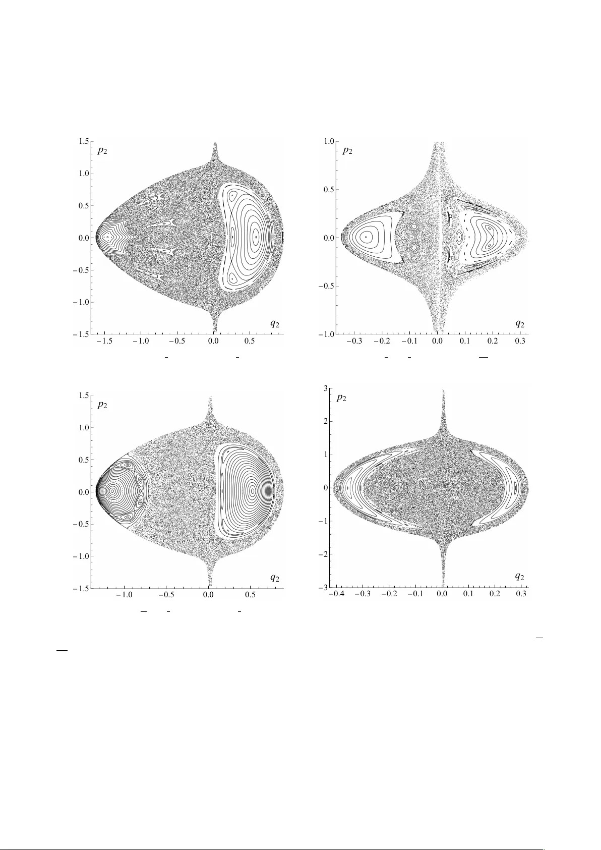
Integ r ability of non-homog eneous Hamilt onian sys tems wit h gyroscopic coupling W ojciech Szumi ´ nski 1 and Andrzej J. Maciejew ski 2 Institute of Ph ysics 1 and Janusz Gil Institute of As tronom y 2 U niv ersity of Zielona G ´ ora, Licealna 9, PL-65–417, Zielona G ´ ora, P oland e-mail: w .szuminski@if.uz.zgor a.pl March 24, 2026 Abstract W e study the integ rability of a tw o-dimensional Hamil- tonian system with a gyroscopic term and a non- homogeneous potential composed of tw o homogeneous components of different degrees. The model describes the motion of a particle in a plane under the combined influ- ence of a centr al (Kepler -type) po tential, a uniform mag- netic field, and a superposition of homogeneous forces. By combining the Levi–Civita regularization with t he so- called coupling constant metamorphosis transformation, and em ploying differential Galois theory , w e deriv e ana- lytical necessary conditions for integrability in t he Liou- ville sense. They put restrictions on the deg rees of homo- geneity of the potential ter ms and their v alues in particu- lar points. The obtained results encom pass and g eneral- ize se v eral classical galactic and astroph ysical models, in- cluding the gener alized Hill model, t he H ´ enon–Heiles and Armbruster–Guck enheimer–Kim systems, providing a uni- fied framew ork for studying non-homogeneous Hamiltoni- ans. W e demonstrate t he effectiv eness of t he deriv ed in- tegrability obstructions b y proving the non-integrability of these models in the presence of a uniform rotational field. The numerical analysis via t he P oincar ´ e cross-sections fur- ther confirms t he analytical results, illustr ating the tran- sition from regular to chaotic dynamics as the rotational and non-homogeneous terms are introduced. Moreov er , w e sho w that, without the Kepler -type term, a gener alized non-homogeneous extension of the excep tional potential remains integrable. The explicit forms of the first integ rals are given. Declaration The article has been published by Nonlin- ear Dynamics in [1], and t he final v ersion is a v ailable at: https://doi.org/10.1007/s11071-026-12309-x 1 Motiv ation and descr iption of t he system The problem of determining whether a giv en dynamical system is integrable or no t is one of the centr al topics in the t heory of differential equations and Hamiltonian sys- tems. While the integ rability of homog eneous potentials has been extensivel y studied and is now relativ ely w ell un- derstood [2 – 4] much less is kno wn about systems that in- clude additional non-homogeneous [5, 6], or gyroscopic terms [7], which natur all y arise in man y ph ysical con- texts. Such systems of ten ser ve as simplified models of galactic dynamics [8, 9], the motion of charged particles in magnetic fields [10], or nonlinear oscillations in rotat- ing frames [11, 12], where the inter pla y betw een symme- try and rotation giv es rise to complex dynamical structures. For a more detailed discussion of these phenomena, see the monograph [13]. In particular , the inclusion of a gyroscopic (Coriolis- like) term fundamentally alters t he dynamics, leading to new mechanisms of resonance and chaos [14 – 16]. A t t he same time, adding a non-homogeneous contribution to the potential breaks t he scaling symmetry that usually facili- tates analytical integ ration [17]. The combined effect of these two perturbations — rotation and non-homogeneity — poses a challenging question regarding t he persis tence or loss of integrability . In t his paper , we address t his problem by analysing a class of tw o–deg ree–of–freedom Hamiltonian system go v - erned by Hamiltonian of the form H µ = 1 2  p 2 1 + p 2 2  + ω ( q 2 p 1 − q 1 p 2 ) − µ r + V ( q 1 , q 2 ) , (1.1) where t he potential V is expressed as V ( q 1 , q 2 ) = V k ( q 1 , q 2 ) + V m ( q 1 , q 2 ) . (1.2) Hamilton equations determined by the Hamilton func- tion (1.1) ha ve the f or m ˙ q 1 = p 1 + ω q 2 , ˙ p 1 = ω p 2 − µ q 1 r 3 − ∂ V ∂ q 1 , ˙ q 2 = p 2 − ω q 1 , ˙ p 2 = − ω p 1 − µ q 2 r 3 − ∂ V ∂ q 2 . (1.3) Here, r = q q 2 1 + q 2 2 denotes the distance from the origin. The functions V i ( q 1 , q 2 ) are assumed to be homogeneous of 1 rational degrees i ∈ Q \ {− 1, 0 } , with k  = m . The parameter µ measures the strength of the central (K epler-type) poten- tial, while ω represents the frequency associated with the gyroscopic ter m. Throughout the main part of t he paper , w e assume µ ω  = 0 , and under t his assump tion, we will de- riv e necessary conditions for the Liouville integrability of the sys tem. The deg enerate case µ = 0 , is treated separ ately in t he final part of the paper . Hamiltonian (1.1) describes the mo tion of a particle in a plane under the combined influence of a central potential − µ / r , tw o homog eneous po tentials V k and V m , and t he gy - roscopic term ω ( q 2 p 1 − q 1 p 2 ) corresponding to motion in a uniforml y rotating reference frame. The gyroscopic term introduces coupling betw een the canonical coordinates and momenta, generating effectiv e magnetic-like forces [18, 19] that significantly alter t he dynamics, consequentl y , t he in- tegrability properties of the system [7, 20]. Ph ysically , Hamiltonian (1.1) represents a broad class of tw o-dimensional galactic and astroph ysical models de- scribing the mo tion of a test particle in a ro tating fr ame [12, 21], see also t he book [22]. The term − µ / r accounts for t he gra vitational attraction of a central mass, whereas t he ho- mogeneous com ponents V k and V m model deviations from spherical symmetry in the g alactic or stellar potential. The presence of the rotational ter m ( ω  = 0 ) produces char acter - istic effects such as resonance capture, bifurcations of peri- odic orbits, and t he formation of stochas tic la yers t hat sep- arate regions of regular mo tion [23 – 25]. Moreov er , Hamiltonian (1.1) admits an equiv alent elec- trodynamic interpretation. It can be written in the com pact v ector form H EM = 1 2  p − A ( q 1 , q 2 )  2 − µ r + V ( q 1 , q 2 ) , (1.4) where A ( q 1 , q 2 ) is t he v ector potential of a uniform mag- netic field B = ∇ × A = 2 ω ˆ z . For the symmetric gaug e A = ( − ω q 2 , ω q 1 , 0 ) , Hamiltonian (1.4) reduces exactl y to (1.1) with V ( q 1 , q 2 ) = 1 2 ω 2  q 2 1 + q 2 2  + V m ( q 1 , q 2 ) . This form rev eals that the rotation term introduces an addi- tional quadr atic contribution to the potential, which breaks its original homogeneity . Hence, the study of the non- homogeneous potential (1.2) is crucial: it captures ho w the combined effects of the magnetic (gyroscopic) field and the nonlinear term V m ( q 1 , q 2 ) modify t he integ rability and dy- namical structure of the system. In t his sense, the same mathematical framew ork describes the planar motion of a charg ed particle in a constant perpendicular magnetic field, subject to a central Coulomb potential and an additional ex- ternal potential V ( q 1 , q 2 ) . Such Hamiltonians g eneralize se v eral classical mod- els in celestial mechanics and galactic dynamics, in- cluding the H ´ enon–Heiles system [26], t he Armbr uster – Guckenheimer –Kim galactic model [27], and t he planar Hill or restricted three-body problems [14, 28, 29]. In all these cases, the interplay betw een t he central potential, t he anisotropic perturbations, and the gyroscopic term giv es rise to rich nonlinear beha viour , ranging from integ rable regimes t o full y dev eloped chaos. Unders tanding ho w the gyroscopic term modifies the integ rability of these systems is therefore essential for explaining the stability of stellar or- bits, the morphology of rotating g alaxies, and t he onset of chaotic transport in gra vitational and electromagnetic sys- tems. The principal goal of this wor k is to determine how the presence of the gyroscopic term alters t he integ rabil- ity conditions of gener alized galactic-type Hamiltonians. In particular , we aim t o identify the forms of the potential V ( q 1 , q 2 ) and parameter combinations ( k , m ) for which sys- tem (1.1) ma y still admit additional meromorphic first in- tegrals. This classification bridges the gap between classi- cal non-rotating integ rable models and their rotating ana- logues, pro viding new insights int o the tr ansition from in- tegrable to chaotic dynamics in low -dimensional Hamilto- nian systems with rotational symmetry . The main result of this paper is f or mulated in the follo w- ing t heorem, which provides necessar y conditions for the Liouville integrability of system (1.1). T o express it in a compact form, w e introduce two auxiliary rational param- eters: n : = 2 − k m − k , l : = 2 + 3 k m − k , (1.5) and define the integr ability coefficients as λ k : = V k ( 1, i ) , λ m : = V m ( 1, i ) . (1.6) W e no te that, in g eneral, λ k , λ m ∈ C . Theorem 1.1 (Main) . Assume that µ ω  = 0 and λ k λ m  = 0 . If sys tem (1.1) is Liouville integr able with mer omor phic firs t inte- grals, t hen: 1. l ≥ − 1 is an odd, or l < − 1 is an even integ er , or 2. ( n + l ) ( n + l + 2 )  = 0 and either (a) n > 0 is an even, or n < 0 is an odd integ er ; or (b) n + l is an even int eg er , excep t the case when l ≥ 0 and n ≤ 0 are bot h even integ ers. Theorem 1.1 establishes t he principal integrability ob- structions f or the gener al case in which both coefficients, λ k and λ m , are nonzero. As will be demonstr ated later , these obstructions are particular ly s trong and highl y effective in practical applications. It is remarkable that they depend solely on the deg rees of homogeneity k and m of t he poten- tial com ponents, and v alues of the potential at the specific complex point ( 1, i ) . How ev er , certain degenerate configur ations occur when one of these coefficients vanishes, leading to qualitativel y different dynamical beha viours that require a separate analysis. In particular , the situation when eit her λ k or λ m is nonzero for n = 0 (corresponding to k = 2 ) demands a more detailed in ves tigation. This is motiv ated b y the exis tence of a special 2 class of non-homogeneous potentials in ph ysics and astron- om y whose lo w er-degree ter m is quadr atic ( k = 2 ). Classi- cal exam ples include the mentioned Hill problem, H ´ enon- Heiles, and t he g eneralized Armbr uster -Guckenheimer- Kim galactic potentials, which share this structure and can be regarded as non-homogeneous potentials with a quadratic leading part. Therefore, t his ex ceptional case is treated separ ately , and t he follo wing tw o theorems pro vide the corresponding obstructions to integ rability . Theorem 1.2. Assume t hat µ ω  = 0 , λ k = 0 , and λ m  = 0 . If k ∈ Q and | m | > 2 , then the sys tem (1.1) is not Liouville integr able wit h mer omorphic fir s t integrals. Theorem 1.3. Assume that µ ω  = 0 , λ k  = 0 , and λ m = 0 . If k = 2 and m ∈ Q , t hen the syst em (1.1) does not admit any meromorphic first integr al functionally independent of the Hamiltonian. In t he abov e t heorems by meromorphic firs t integrals, w e understand complex meromorphic functions of variables ( q 1 , q 2 , p 1 , p 2 , r ) . The proofs of Theorems 1.1–1.3 are based on the Morales–Ramis t heory [30, 31], which pro vides one of the most effectiv e analytical tools for studying the (non- )integrability of Hamiltonian systems. This approach link s the classical idea of linearisation around a particular solu- tion wit h the modern framew ork of differential Galois the- ory , establishing a direct correspondence betw een t he alge- braic structure of the variational equations and the dynam- ical properties of the original nonlinear system [32, 33]. The central result in t his context w as established b y Morales and Ramis [31], who prov ed that Liouville inte- grability im poses strong alg ebraic constr aints on the Galois group of the v ariational equations. Theorem 1.4 (Morales–Ramis, 1999) . Let a complex Hamil- tonian syst em with n degrees of freedom be Liouville integr able with meromorphic first integr als in a neighbourhood of a non- equilibrium phase curve Γ . Then, t he identity component of the differential Galois gr oup of t he variational equations along Γ is Abelian. This theorem provides a necessary condition for inte- grability and serves as t he basis of most modern non- integrability proofs. In practice, its application follo ws a relativ ely standar d sequence of steps: first, one identifies a particular solution Γ ( t ) of equations of motion (1.3) gen- erated b y Hamiltonian (1.1). Next, t he equations of mo- tion are linearised along this tra jector y to obtain the v aria- tional equations. F inall y , one analyzes the differential Ga- lois group of t hese equations. If t he identity component of this group is shown to be non- Abelian, t hen, b y Theo- rem 1.4, the original system cannot be Liouville integ rable. T o prov e Theorems 1.1 – 1.3, w e t herefore construct an appropriate particular solution of t he system (1.3) and demonstr ate that the associated variational equations pos- sess a non- Abelian Galois group. The explicit construction of t his solution and t he deriv ation of t he corresponding v ariational equations are discussed in the next section. It should be emphasised t hat, in gener al, there is no sys- tematic or algorit hmic met hod for selecting a tr ajectory Γ ( t ) suitable for t he application of the Morales–Ramis theor y . Ev en when such a tra jector y is known, t he subsequent anal- ysis of the differential Galois g roup is often highly non- trivial. In most cases, t he variational equations do no t de- couple into low er -dimensional subsystems, and their Ga- lois groups must be s tudied case b y case using a combina- tion of alg ebraic and anal ytic ar guments. A com prehensive exposition of the theory and its appli- cations can be found in t he w or k s of Morales and Ramis [30, 31] and t he monog raph by A udin [33]. For an accessi- ble introduction wit h w orked examples, see also [34]. The Morales–Ramis frame w ork has become a standar d t ool for detecting non-integrability , and it has been successfully ap- plied to a wide v ariety of problems — ranging from the clas- sical three-body problem [35 – 37], n -body problem [38] to modern models in g alactic dynamics [39]. N umerous o t her applications of this t heory in recent years can be found in [40 – 51]. Follo wing the assumptions of Theorem 1.4, w e consider the complexified v ersion of our system, ( q 1 , q 2 , p 1 , p 2 ) ∈ C 4 , with t he potential V ( q 1 , q 2 ) assumed to be algebr aic ov er C ( q 1 , q 2 ) . Alt hough t he Hamiltonian (1.1) is not strictly meromorphic because of the term − µ / r = − µ / q q 2 1 + q 2 2 , it has been shown in [52, 53] t hat t he Morales–Ramis t he- ory can s till be consistentl y applied to such sys tems, pro- vided that t he singularities of the potential are handled within t he framew or k of algebr aic differential equations. How ev er , w e av oid difficulties just b y considering integra- bility in ter ms of complex meromorphic functions of v ari- ables ( q 1 , q 2 , p 1 , p 2 , r ) . Moreov er , t he application of the Levi- Civita transf or mation reduced the problem to studying t he integrability of systems wit h a r ational Hamiltonian func- tion. The rest of t he paper is or ganized as follo ws. In Sec. 2 w e construct explicit particular solutions of the Hamiltonian H µ , using the Levi–Civita regularization combined with the coupling–constant metamorphosis. W e then deriv e the variational equations restricted to an in v ariant plane and rewrite them as tw o second-or der reduced differential equations: a homogeneous Gauss hyper geometric equa- tion and a non-homogeneous equation sharing the same homogeneous part. In Secs. 3 – 5 w e analyse the integ rabil- ity of t he reduced variational equations via differential Ga- lois t heory and monodromy of t he Gauss h ypergeometric equation and its degenerate cases, identifying all admissi- ble configurations for which the identity component of the Galois group is A belian. These sections contain the proofs of Theorems 1.1 – 1.3. Sec. 6 applies t he obtained integ rabil- ity obstructions to sev eral classical models, including the gener alized Hill, the H ´ enon–Heiles, and t he Armbruster – Guckenheimer –Kim systems, and illustrates the analytical results with representativ e P oincar ´ e cross-sections. Sec. 7 departs from t he obs truction-based anal ysis and examines the special case µ = 0 , where Hamiltonian (1.1) reduces to t he rotating Hamiltonian H 0 . In this regime t he regu- 3 larisation is no longer equivalent to t he original dynam- ics, so Theorems 1.1–1.3 do not apply , and t he Morales– Ramis met hod cannot be used due to t he lack of an ap- propriate particular solution. N ev ertheless, w e sho w t hat the rotating Hamiltonian H 0 with a non-homogeneous ex- ceptional po tential becomes super-integrable; Sec. 7 estab- lishes this b y cons tructing tw o additional independent first integrals. Sec. 8 pro vides concluding remar k s and out- lines furt her perspectiv es. The paper ends wit h tw o ap- pendices: Appendix A formulates the anal ytic criterion de- termining when the identity component of the differential Galois group of the reduced v ariational sys tem is Abelian, while Appendix B presents the monodromy anal ysis of t he relev ant Gauss hyperg eometric equation, including local monodrom y matrices, connection formulas, and the loga- rithmic cases required in se ver al proofs. 2 P ar ticular solutions and variational equations As noted abov e, the Morales–Ramis approach requires the existence of a non-equilibrium particular solution of the equations of motion. Since no gener al method for con- structing such solutions is a v ailable, w e emplo y a sequence of canonical tr ansformations adapted to t he structure of the Hamiltonian system under consider ation. W e emphasize t hat these transf or mations are no t intro- duced solel y to regularize t he Kepler -type term − µ / r , as the Morales–Ramis theor y is also applicable to Hamiltonian systems with alg ebraic potentials. Their primar y pur pose is to identify in v ariant manifolds and to construct an ex- plicit particular solution of the system (1.3) along which the Morales–Ramis integ rability anal ysis can be effectivel y carried out. With this aim, w e first appl y t he Levi–Civita transf orma- tion, which yields a Hamiltonian form suitable for the sub- sequent application of t he coupling constant metamorpho- sis. N amely q 1 = u 2 1 − u 2 2 , p 1 = u 1 v 1 − u 2 v 2 2 ( u 2 1 + u 2 2 ) , q 2 = 2 u 1 u 2 , p 2 = u 1 v 2 + u 2 v 1 2 ( u 2 1 + u 2 2 ) . (2.1) Hamiltonian (1.1) in these new coordinates now reads e K µ = v 2 1 + v 2 2 8 ( u 2 1 + u 2 2 ) + ω 2 ( u 2 v 1 − u 1 v 2 ) − µ u 2 1 + u 2 2 + U ( u 1 , u 2 ) , (2.2) where U ( u 1 , u 2 ) = V ( u 2 1 − u 2 2 , 2 u 1 u 2 ) . The corresponding equations of motion are as f ollows ˙ u 1 = ∂ e K µ ∂ v 1 = v 1 4 ( u 2 1 + u 2 2 ) + ω 2 u 2 , ˙ u 2 = ∂ e K µ ∂ v 2 = v 2 4 ( u 2 1 + u 2 2 ) − ω 2 u 1 , ˙ v 1 = − ∂ e K µ ∂ u 1 = ( v 2 1 + v 2 2 ) u 1 4 ( u 2 1 + u 2 2 ) 2 + ω 2 v 2 − 2 µ u 1 ( u 2 1 + u 2 2 ) 2 − ∂ U ∂ u 1 , ˙ v 2 = − ∂ e K µ ∂ u 2 = ( v 2 1 + v 2 2 ) u 2 4 ( u 2 1 + u 2 2 ) 2 − ω 2 v 1 − 2 µ u 2 ( u 2 1 + u 2 2 ) 2 − ∂ U ∂ u 2 . For t he next s tep, w e used the follo wing lemma, which w as prov ed in [54], see also [55, 56]. Lemma 2.1. Assume that Hamiltonian gener at es a Hamiltonian sys tem wit h n degrees of freedom F ( q , p , α ) = F 0 ( q , p ) − α F 1 ( q , p ) has a firs t integral I ( q , p , α ) functionally independent of F . Then, the sys tem with Hamiltonian G ( q , p , f ) = F 0 ( q , p ) − f F 1 ( q , p ) has a firs t int egr al J ( q , p , f ) = I ( q , p , G ( q , p , f ) ) . Let us apply this lemma to t he Hamiltonian (2.2). W e ha ve F 0 ( u , v ) = v 2 1 + v 2 2 8 ( u 2 1 + u 2 2 ) + ω 2 ( u 2 v 1 − u 1 v 2 ) + U ( u 1 , u 2 ) , F 1 ( u , v ) = 1 4 ( u 2 1 + u 2 2 ) , and α = 4 µ , f = h . Denoting K ( u , v ) = G ( u , v , h ) , w e obtain K ( u , v ) = 1 2 ( v 2 1 + v 2 2 ) + 2 ( u 2 1 + u 2 2 ) ω ( u 2 v 1 − u 1 v 2 ) (2.3) + 4 ( u 2 1 + u 2 2 )( U ( u 1 , u 2 ) − h ) . (2.4) Equations of motion generated b y Hamiltonian (2.3) ad- mit inv ariant planes. T o sim plify their forms, w e perf or m the additional canonical change of the variables u 1 = x 1 + i x 2 √ 2 , u 2 = i x 1 + x 2 √ 2 , v 1 = y 1 − i y 2 √ 2 , v 2 = − i y 1 + y 2 √ 2 . (2.5) After this transformation, the Hamiltonian K 0 takes t he form e K = − i ( y 1 y 2 + 8 hx 1 x 2 ) + 4 ω x 1 x 2 ( x 2 y 2 − x 1 y 1 ) + 8i x 1 x 2 e V ( x 1 , x 2 ) , (2.6) where e V ( x 1 , x 2 ) = V ( x 2 1 − x 2 2 , i ( x 2 1 + x 2 2 )) . The corresponding equations of mo tion are as follow s ˙ x 1 = − i y 2 − 4 ω x 2 1 x 2 , ˙ x 2 = − i y 1 + 4 ω x 1 x 2 2 , ˙ y 1 = 4 x 2 ω ( 2 x 1 y 1 − x 2 y 2 ) + 8i x 2 h − e V ( x 1 , x 2 ) − x 1 ∂ e V ( x 1 , x 2 ) ∂ x 1 ! , ˙ y 2 = 4 x 1 ω ( x 1 y 1 − 2 x 2 y 2 ) + 8i x 1 h − e V ( x 1 , x 2 ) − x 2 ∂ e V ( x 1 , x 2 ) ∂ x 2 ! . 4 (2.7) N o w , it is evident t hat the system (2.7) possesses tw o sim- ple inv ariant planes, which are giv en b y M 1 =  ( x 1 , x 2 , y 1 , y 2 ) ∈ C 4   x 2 = y 1 = 0  , M 2 =  ( x 1 , x 2 , y 1 , y 2 ) ∈ C 4   x 1 = y 2 = 0  . (2.8) For further analysis, w e restrict the sys tem t o the firs t plane ˙ x 1 = − i y 2 , ˙ y 2 = 8i h h − e V ( x 1 , 0 ) i x 1 . (2.9) Knowing t hat e V ( x 1 , 0 ) = V ( x 2 1 , i x 2 1 ) and V is a sum of two ho- mogeneous functions V k and V m , w e obtain the differential equation ¨ x 1 − 8 h h − λ k x 2 k 1 − λ m x 2 m 1 i x 1 = 0, (2.10) where in the last step, we ha v e used t he homog eneity prop- erty V i ( x 2 1 , i x 2 1 ) = λ i x 2 i 1 , where λ i : = V i ( 1, i ) . Assuming t hat k , m ∈ {− 1, 0 } , w e find t hat Eq. (2.10) has the first integral of t he form I = 1 2 ˙ x 2 1 + 4 x 2 1  λ k k + 1 x 2 k 1 + λ m m + 1 x 2 m 1 − h  . (2.11) The function I can be treated as t he conser vation of t he en- ergy of the sys tem (2.10), where I = e is its lev el. Let X = [ X 1 , Y 2 , X 2 , Y 1 ] T denotes t he v ariations of x = [ x 1 , y 2 , x 2 , y 1 ] T , then the variational equations restricted to M 1 , are as follo ws d d τ X = A ( τ ) X , (2.12) with a non-constant matrix A ( τ ) =     0, − i − 4 ω x 2 1 0 a 12 0 − 8i ω x 1 ˙ x 1 4 ω x 2 1 0 0 0 − i 0 0 a 12 0     , where a 12 = 4i ( 2 h − 2 ( 1 + 2 k ) λ k x 2 k 1 − 2 ( 1 + 2 m ) λ m x 2 m 1 ) . In the abov e calculations, we used t he Euler identity for homoge- neous functions. For instance for V k , we write x 1 ∂ V k ∂ x 1 + x 2 ∂ V k ∂ x 2 = k V k , (2.13) which enables x 2 1 ∂ V k ∂ x 1 ( x 2 1 , i x 2 1 ) + i x 2 1 ∂ V k ∂ x 2 ( x 2 1 , i x 2 1 ) =  ∂ V k ∂ x 1 ( 1, i ) + i ∂ V k ∂ x 2 ( 1, i )  x 2 k 1 = k λ k x 2 k 1 . (2.14) V ariational equations (2.12) form a sys tem of four first- order differential equations. For better readability , w e rewrite it as a system of tw o second-or der differential equa- tions ¨ X 2 + a ( τ ) X 2 = 0, (2.15a) ¨ X 1 + a ( τ ) X 1 = b ( τ ) X 2 , (2.15b) where a ( τ ) = − 8 h h − ( 1 + 2 k ) λ k x 2 k 1 − ( 1 + 2 m ) λ m x 2 m 1 i , b ( τ ) = − 16 ω x 1 ˙ x 1 . These coefficients are functions defined on the hyper - elliptic curve ˙ x 2 1 = 2 e + 8 hx 2 1 − 8 λ k k + 1 x 2 ( k + 1 ) 1 − 8 λ m m + 1 x 2 ( m + 1 ) 1 . (2.16) T o simplify further com putations, w e set h = e = 0 , and as- sume λ k λ m  = 0 , that is V k ( 1, i ) V m ( 1, i )  = 0 . Thanks to t his, the change of the independent variable τ → z = 1 + ( 1 + k ) λ m ( 1 + m ) λ k ( x 1 ( τ ) ) 2 ( m − k ) , (2.17) tog ether with tr ansformation rules for t he derivativ es d d τ = ˙ z d d z , d 2 d τ 2 = ˙ z 2 d 2 d z 2 + ¨ z d d z , (2.18) con vert the variational equations (2.15) into the follo wing forms X ′′ 2 + p ( z ) X ′ 2 + q ( z ) X 2 = 0, (2.19a) X ′′ 1 + p ( z ) X ′ 1 + q ( z ) X 1 = s ( z ) X 2 . (2.19b) Here, p ( z ) , q ( z ) , and s ( z ) are non-constant rational func- tions, given b y p ( z ) = ¨ z ˙ z 2 = 1 2  1 z + n − l − 8 4 ( 1 − z )  , q ( z ) = a ( z ) ˙ z 2 = 1 32  n 2 − 2 nl − 15 l 2 8 ( 1 − z ) 2 + 16 + n + 11 l z ( 1 − z )  , s ( z ) = b ( z ) ˙ z 2 = Ω ( 1 − z ) n − 4 2 √ z , Ω ∈ C \ { 0 } , where n , l ∈ Q are auxiliar y parameters previousl y intro- duced in (1.5). N o w , w e mak e the classical T schirnhaus tr ansformation of dependent v ariables X 2 = X e xp  − 1 2 Z p ( z ) d z  , X 1 = Y exp  − 1 2 Z p ( z ) d z  , (2.20) Thanks to that, w e can rewrite (2.19a)-(2.19b) to their re- duced forms X ′′ = r ( z ) X , (2.21a) Y ′′ = r ( z ) Y + s ( z ) X . (2.21b) 5 The coefficients of the abov e system are r ( z ) = 1 4  ρ 2 − 1 z 2 + σ 2 − 1 ( 1 − z ) 2 − 1 − ρ 2 − σ 2 + τ 2 z ( 1 − z )  , s ( z ) = Ω ( 1 − z ) n − 4 2 √ z , Ω ∈ C \ { 0 } (2.22) Here ρ , σ , τ are the differences of the exponents of Gauss differential equation (2.21a), wit h v alues ρ = 1 2 , σ = l 2 , τ = 3 + l 2 . (2.23) The respective exponents are giv en by ρ 1,2 = 1 ± ρ 2 , σ 1,2 = 1 ± σ 2 , τ 1,2 = − 1 ± τ 2 . Equation (2.21a) is reducible as − ρ − σ + τ = 1, (2.24) see Appendix B. Its one solution is alg ebraic, and it has the follo wing f or m. x 1 ( z ) = z 3 / 4 ( 1 − z ) 2 + l 4 , (2.25) the second one is giv en b y x 2 ( z ) = x 1 ( z ) Z 1 x 1 ( z ) 2 d z = 4 √ z ( 1 − z ) 2 + l 4 F  − 1 2 , 1 + l 2 ; 1 2 ; z  . (2.26) Here F ( α , β ; γ ; z ) : = 2 F 1 ( α , β ; γ ; z ) , is the Gaussian h yperge- ometric function; f or details, see Appendix B. 2.1 Case k = 2 and λ k = 0, and λ m  = 0 Let us assume h  = 0 . Then we perform the follo wing change of t he independent variable τ 7− → z = 1 − λ m ( m + 1 ) h ( x 1 ( τ )) 2 m , at e = 0. (2.27) This change of v ariables, together wit h transf ormations of deriv ativ es (2.18), conv ert t he system (2.15) to the rational form (2.19), wit h the coefficients p ( z ) = ¨ z ˙ z 2 = 3 z − 1 2 ( z − 1 ) z , q ( z ) = a ( z ) ˙ z 2 = − m ( 2 m + 3 ) ( z − 1 ) + z 4 m 2 ( z − 1 ) 2 z , s ( z ) = b ( z ) ˙ z 2 = Ω ( 1 − z ) 1 m − 2 √ z , Ω ∈ C \ { 0 } . (2.28) After the T schir nhaus transformation, w e obtain t he re- duced f or m of t he v ariational equations (2.21), wit h the co- efficients r ( z ) = − 3 m 2 + ( m + 2 ) ( 5 m + 2 ) z 2 − 6 ( m + 2 ) mz 16 m 2 ( z − 1 ) 2 z 2 , s ( z ) = Ω ( 1 − z ) 1 m − 2 √ z . (2.29) With these coefficients, equation (2.21a) is reducible. Its algebr aic solution is x 1 ( z ) = z 3 / 4 ( 1 − z ) m + 1 2 m . (2.30) The second solution is x 2 ( z ) = x 1 ( z ) ψ ( z ) where ψ ( z ) = Z 1 x 1 ( z ) 2 d z = − 2 √ z F  − 1 2 , 1 + 1 m ; 1 2 ; z  (2.31) Moreov er , integrals ϕ ( z ) and I ( z ) defined in (A3) take the forms ϕ ( z ) = − m Ω ( 1 − z ) 2 / m ( m + 2 z ) 2 ( m + 2 ) , I ( z ) = Z ϕ ( z ) ψ ( z ) d z = a ( z ) + b √ zF  1 2 , 1 − 1 m ; 3 2 ; z  (2.32) where a ( z ) is an algebr aic function and b is a non-zero con- stant (t heir explicit forms are irrelev ant for our further con- siderations). 2.2 Case k = 2 and λ k  = 0, and λ m = 0 Let us assume h  = 0 . Then we perform the follo wing change of t he independent variable τ → z = v u u t 1 − 2 s h λ k x − 2 1 ( τ ) , at e = 8 3 s h 3 λ k . (2.33) This change of variables, combined with the deriv ative transf ormations giv en in (2.18), recasts the system (2.15) into t he rational form (2.19), wit h the coefficients p ( z ) = ¨ z ˙ z 2 = 2 z z 2 − 3 , q ( z ) = a ( z ) ˙ z 2 = 3 ( z 4 − 2 z 2 − 19 ) ( z 2 − 1 ) 2 ( z 2 − 3 ) 2 , s ( z ) = b ( z ) ˙ z 2 = Ω z ( z 2 − 3 )( z 2 − 1 ) 2 , Ω ∈ C \ { 0 } . (2.34) P erforming t he T schirnhaus transf ormation of dependent v ariables (2.20), w e obtain the reduced f orm of the v aria- tional equations (2.21), with the coefficients r ( z ) = − 6 ( z 4 − 2 z 2 − 9 ) ( z 2 − 1 ) 2 ( z 2 − 3 ) , s ( z ) = 3 Ω z ( z 2 − 3 )( z 2 − 1 ) 2 . (2.35) With these coefficients, equation (2.21a) is reducible. Its algebr aic solution is x 1 ( z ) = z ( z 2 − 3 ) ( z 2 − 1 ) 3 / 2 . (2.36) The second solution is x 2 ( z ) = x 1 ( z ) ψ ( z ) where ψ ( z ) = Z 1 x 1 ( z ) 2 d z = − 4 z 4 + 11 z 2 − 3 9 z ( z 2 − 3 ) 2 (2.37) − 5 9 √ 3 arctanh  z √ 3  (2.38) 6 Moreov er , integrals ϕ ( z ) and I ( z ) defined in (A3) take the forms ϕ ( z ) = Ω  − 2 z 6 + 9 z 4 − 12 z 2 + 3  4 ( z 2 − 1 ) 4 , I ( z ) = Z ϕ ( z ) ψ ( z ) d z = 1 288 Ω " 3  z 4 + 7 z 2 − 24  z ( z 2 − 3 ) 2 − 18 arctanh ( z ) + 5 √ 3 arctanh  z √ 3  . (2.39) 3 Proofs of Theorems 1.1 – 1.3 The proof of Theorem 1.1 is based on the following lemma. Lemma 3.1. F or l , n ∈ Q , t he identity com ponent of the differ - ential Galois gr oup of t he sys tem (2.21) is Abelian if and only if 1. l ≥ − 1 is an odd, or l < − 1 is an even integ er , or 2. ( n + l ) ( n + l + 2 )  = 0 and either (a) n > 0 is an even, or n < 0 is an odd integ er ; or (b) n + l is an even int eg er , excep t the case when l ≥ 0 and n ≤ 0 are bot h even integ ers. W e will pro v e it in t he next section. Firs t, w e show t he follo wing fact. Theorem 3.2. Under the assumptions of Theor em 1.1, if the sy s- tem governed by Hamiltonian (2.3) is int egrable in the Liouville sense with meromorphic fir s t integrals, t hen: 1. l ≥ − 1 is an odd, or l < − 1 is an even integ er , or 2. ( n + l ) ( n + l + 2 )  = 0 and either (a) n > 0 is an even, or n < 0 is an odd integ er ; or (b) n + l is an even int eg er , excep t the case when l ≥ 0 and n ≤ 0 are bot h even integ ers. Proof. The system gov erned b y Hamiltonian (2.3) has a famil y of particular solutions defined b y (2.9), or equiv a- lently b y (2.10), and t he corresponding v ariational equa- tions are given by (2.15). If it is integ rable, then according to the Morales-Ramis Theorem 1.4, the identity com ponent of the differential Galois group of t he v ariational equations along the mentioned particular solution is Abelian. In v ok - ing Lemma 3.1, w e obtain the thesis of the theorem. N o w , the proof of Theorem 1.1 is simple. Proof. [Proof of Theorem 1.1] Let us assume t hat the system defined Hamilt onian (1.1) is integrable. Then it admits an additional first integ ral, which is a meromor phic function of ( q 1 , q 2 , p 1 , p 2 , r ) . Af ter the Levi-Civita transformation, it will be a meromorphic function of ( u 1 , u 2 , v 1 , v 2 ) which is an additional first integral system defined b y Hamilto- nian (2.2). Thus, b y b y Lemma 2.1, the system gov er ned b y Hamiltonian (2.3) is integ rable. But by Theorem 3.2 states that it is not integ rable. The contradiction finishes the proof. W e pass now to t he proof of Theorem 1.2. The proof is based on t he f ollo wing lemma which w e prov e in Section 5. Lemma 3.3. If | m | > 2 t hen the identity component of t he differ - ential Galois group of t he sys tem (2.21) with coefficients defined by (2.29) is no t Abelian. With t he abov e lemma, the proof of Theorem 1.2 is simi- lar as the proof of Theorem 1.1 and w e left it to the reader . Proof of Theorem 1.3 needs more effort. Proof. [Proof of Theorem 1.3] As in t he proof of Theo- rem 1.1, first we in ves tigate integ rability t he system defined b y Hamiltonian (1.1). T o this end is integrable, variational equations along a particular solution defined b y (2.9). They are giv en b y (2.21), with coefficients defined b y (2.35). T o show that t he identity component of its differential Galois group is not Abelian, we apply Lemma A.3. T aking. into ac- count t hat for t he considered case functions ψ ( z ) and I ( z ) are giv en b y ( ?? ) and (2.39), w e find t hat function g ( z ) de- fined by (A5) has the follo wing form g ( z ) = R ( z ) + ( λ c 1 + c 2 ) arctanh  z √ 3  + c 3 arctanh ( z ) where R ( z ) is a r ational function, and c 1 , c 2 and c 3 are non- zero constants. For arbitr ar y λ ∈ C , this function is not al- gebr aic. T o see this, w e no te t hat if g ( z ) is algebraic, then the function e g ( z ) = a 1 arctanh  z √ 3  + a 2 arctanh ( z ) , is algebraic for some a 1 , a 2 ∈ C , not both zero. This is impos- sible because an alg ebraic function does not ha ve irregular singularities. If a 1  = 0 then arctanh ( z / √ 3 ) as well as e g ( z ) has tw o irregular singular points at z = ± √ 3 . Thus, neces- sarily a 1 = 0 . In our case a 1 = λ c 1 + c 2 , so w e ha ve to fix λ = − c 2 / c 1 . Ho w ev er , if a 2  = 0 , t hen arctanh ( z ) and e g ( z ) has tw o irregular singular points at z = ± 1 . Thus, necessar - ily a 2 = 0 . This is a contradiction which prov es our state- ment. Thus, the identity component of t he differential Ga- lois group of t he v ariational equations is not Abelian, which finishes t he proof of Theorem 1.3. 4 Main lemma In t his section, we formulate and prov e the Lemma 3.1 which pla ys a key role in the proof of Theorem 1.1. It spec- ifies all cases when the identity component of the sys tem’s differential Galois group of the sys tem (2.21) is A belian. T o prov e t his lemma, w e use the criteria formulated in Appendix A. T o this end w e must compute t he integ rals ψ ( z ) , ϕ ( z ) , and I ( z ) defined in (A3). The functions r ( z ) and s ( z ) for t he system (2.21) are giv en by (2.22). The integral ψ ( z ) is ψ ( z ) = − 2 √ z F  − 1 2 , 1 + l 2 ; 1 2 ; z  . (4.1) If t his function is algebraic, then the tw o solutions of equa- tion (2.21a) are algebr aic, and t he identity component of 7 the differential Galois g roup of system (2.21) is Abelian; see Lemma A.1. Note t hat ψ ( z ) is alg ebraic if and onl y if the solution x 2 ( z ) giv en by (2.26) is alg ebraic. W e sho w first the f ollowing facts. Proposition 4.1. Solution (2.26) is algebr aic if and onl y if eit her l ≥ − 1 is an odd int eg er , or l < − 1 is an even integer . In t his case, t he identity com ponent of t he differ ential Galois group of t he sys tem (2.21) is Abelian. Proof. If solution (2.26) is algebr aic, then it has the form x 2 ( z ) = z e 0 ( z − 1 ) e 1 p ( z ) (4.2) where p ( z ) is a pol ynomial of degree d = − ( e 0 + e 1 + e ∞ ) , and e 0 , e 1 and e ∞ are exponents at the points 0 , 1 , and ∞ re- spectiv ely , see [57, Ch.4]. From this fact, w e deduce t hat l has to be an integer . This is onl y a necessar y condition. If l is an integer , t hen solution (2.26) can ha v e a log arit hmic ter m. The necessar y and sufficient condition for t he presence of logarithmic term is giv en in [57, Lemma 4.3.7]. Using them, w e find t hey do no t appear if and only if l satisfies the giv en assump tions. If both solutions of equation (2.21a) are algebraic, then, as the equation is reducible, its differential Galois g roup, as w ell as the monodrom y group, is contained in t he diago- nal subgroup of SL ( 2, C ) . Then by Theorem 3.2 in [58], t he identity component of t he differential Galois group of t he system (2.21) is Abelian. The form of integ ral ϕ ( z ) defined by (A3) depends on the v alues of n and l . N amel y , if ( n + l ) ( n + l + 2 )  = 0 , then ϕ ( z ) is algebr aic ϕ ( z ) = − 2 Ω [ 2 + z ( n + l ) ] ( 1 − z ) n + l 2 ( n + l ) ( n + l + 2 ) . (4.3) In t his case, w e need also the integ ral I ( z ) , which is given b y I ( z ) = a ( z ) + b √ zF  1 2 , 1 − n 2 ; 3 2 ; z  , (4.4) where a ( z ) is an algebr aic function and b is a non-zero com- plex number (The explicit form of t hese coefficients is irrel- ev ant f or further calculations). The case when ( n + l ) ( n + l + 2 ) = 0 correspond t o k = − 2 or m = − 2 . If l = − n , t hen ϕ ( z ) = − a ( z + log ( z − 1 ) ) (4.5) and if l = − n − 2 , then ϕ ( z ) = a  log ( z − 1 ) − 1 z − 1  . (4.6) In both cases, function ϕ ( z ) is no t alg ebraic. The proof of Lemma 3.1 depends on the condition ( n + l )( n + l + 2 )  = 0 . 4.1 The algebraic case This section assumes that ( n + l )( n + l + 2 )  = 0 . As f or cases considered in this section, ϕ ( z ) is alg ebraic, w e will use criterion giv en in Lemma A.3. Since inte- grals ψ ( z ) and I ( z ) are giv en by (4.1) and (4.4), it is clear that, after the rearrang ement of terms, as a function g ( z ) in Lemma A.3 we can take g ( z ) : = λ F ( α , β ; γ ; z ) + zF ( b α , b β ; b γ ; z ) , (4.7) where ( α , β , γ ) =  − 1 2 , 1 + l 2 , 1 2  , ( b α , b β , b γ ) =  1 2 , 1 − n 2 , 3 2  . (4.8) W e hav e to check if there exists λ ∈ C such t hat g ( z ) is alge- braic. Let us notice that if F ( b α , b β ; b γ ; z ) is algebraic, t hen g ( z ) is algebr aic as w ell for λ = 0 . In these cases, w e distinguish b y t he follo wing proposition. Proposition 4.2. The hyper g eometric function F  1 2 , 1 − n 2 ; 3 2 ; z  is algebr aic if and only if either n is positive and even, or n is negativ e and odd. The proof of this proposition is similar to the proof Proposition 4.1, so w e omit it. T o verify if g ( z ) is algebr aic, w e in ves tigate its analytic continuations along closed paths with a common one point. If it is an algebr aic function, then such continuations can giv e only a finite number of different v alues. As g ( z ) is a linear combination of two h ypergeometric functions, w e ha ve to anal yse the analytical continuations of both of them. Thus, w e ha v e to analyse tw o Gauss h ypergeometric equa- tions with respectiv e parameters ( α , β , γ ) and ( b α , b β , b γ ) . The respectiv e bases of local solutions in a neighbourhood of singularity z = 0 are u 1 ( z ) = F ( α , β ; γ ; z ) , u 2 ( z ) = √ z , b u 1 ( z ) = F ( b α , b β ; b γ ; z ) , b u 2 ( z ) = 1 √ z . W e shall check how t hese local solutions change during an- alytical continuation along certain closed loops. No tions of analytical continuation and local and global monodrom y and their calculations f or the h yperg eometric equation are presented in Appendix B. W e take tw o loops σ 0 and σ 1 with one common point z 0 encircling counter-clockwise singularities z = 0 and z = 1 , respectiv ely , see Fig. 6 in Appendix A . By M σ 0 and M σ 1 w e denote the respectiv e monodrom y matrices. Let us assume t hat neither l nor n is an ev en integer . Then the An explicit form of monodrom y matrices is de- fined b y (A7) and (A15). For further considerations, we take t he commutator loop ρ 1 = σ 0 σ 1 σ − 1 0 σ − 1 1 and t he corresponding monodromy matrix C : = M ρ 1 = M − 1 σ 1 M − 1 σ 0 M σ 1 M σ 0 (4.9) 8 W e will also need the follo wing commutator D : = M ρ ∞ = M − 1 σ ∞ M − 1 σ 0 M σ ∞ M σ 0 (4.10) For the sets of parameters (4.8), the respectiv e commuta- tor matrices are denoted b y C , b C and D , b D . All of them are unipotent and lo w er triangular , thus t hey hav e the form C =  1 0 c 21 1  , b C =  1 0 b c 21 1  , D =  1 0 d 21 1  , b D =  1 0 b d 21 1  . The anal ytical continuations of F ( α , β ; γ ; z ) and F ( b α , b β ; b γ ; z ) along loop ρ 1 giv e M ρ 1 ( F ( α , β ; γ ; z ) ) = F ( α , β ; γ ; z ) + c 21 √ z , M ρ 1 ( F ( b α , b β ; b γ ; z ) ) = F ( b α , b β ; b γ ; z ) + b c 21 1 √ z . Hence M ρ 1 ( g ( z ) ) = λ M ρ 1 ( F ( α , β ; γ ; z ) ) + z M ρ 1 ( F ( b α , b β ; b γ ; z ) ) = g ( z ) + √ z ∆ 1 , where ∆ 1 : = λ c 21 + b c 21 . If ∆ 1  = 0 then continuation along loops ρ N 1 giv e finitely man y v alues of g ( z ) as w e ha v e M ρ ( g ( z ) ) = g ( z ) + N √ z ∆ 1 , for N ∈ Z . Thus, if g ( z ) is algebr aic, t hen ∆ 1 = 0 . But this one con- dition is not sufficient. In fact, ∆ 1 = 0 for λ = − b c 21 / c 21 . This is wh y w e should consider the commutator D . Sim- ilar reasoning wit h analytical continuation along loop ρ ∞ giv es M ρ ∞ ( g ( z ) ) = g ( z ) + √ z ∆ ∞ , where ∆ ∞ : = λ d 21 + b d 21 . Summarizing, if g ( z ) is algebr aic, then ∆ 1 = 0 and ∆ ∞ = 0 , that is, there exists λ ∈ C such that λ c 21 + b c 21 = 0, λ d 21 + b d 21 = 0. It is possible if and onl y if the follo wing determinant ∆ = det  c 21 b c 21 d 21 b d 21  (4.11) v anishes. The explicit form of the non-trivial elements of the commutator matrices C , b C , D , and b D are f ollowing c 21 = e − i π l d 21 , b c 21 = − √ π  1 − e i n π  Γ  n 2  Γ  1 + n 2  , d 21 = 2 √ π  1 − e i π l  Γ  − l 2  Γ  − l + 1 2  , b d 21 = e − i π n b c 21 . With t hese formulae, w e obtain ∆ = R e − i π ( l + n )  e i π l − 1   e i π n − 1   e i π ( l + n ) − 1  , (4.12) where R is giv en b y R = − 2 π Γ  − l 2  Γ  n 2  Γ  − l + 1 2  Γ  n + 1 2  . (4.13) By our assum ptions, R  = 0 . Hence, if g ( z ) is algebr aic, t hen ∆ = 0 . Since neit her l nor n is an ev en integer , from (4.12) we deduce that ∆ = 0 if and onl y if n + l is an ev en integer . This completes t he proof of Lemma 3.1 in the case ( n + l ) ( n + l + 2 )  = 0 with neither n nor l being an ev en integer . W e ha v e to in v estigate t he cases when l or n is an ev en integer . A t first, let us assume t hat l = 2 l ′ is an e v en integer . Moreov er , w e assume also that n is neither an ev en positiv e nor a negativ e and odd integer . This guar antees that t he function b u 1 ( z ) = F  1 2 , 1 − n 2 ; 3 2 ; z  is no t alg ebraic, see Propo- sition 4.2. If l = 2 l ′ < − 1 , then the statement 1 of Lemma 3.1 follo ws from Proposition 4.1. Thus, w e assume that l = 2 l ′ ≥ 0 is an ev en integ er , so ( α , β , γ ) = ( − 1 2 , 1 + l ′ , 1 2 ) . For these pa- rameters the respective local monodrom y matrix at z = 1 is e M σ 1 =  1 0 2 π i 1  . Hence, for any non-zero integer ν we hav e e M ν σ 1 =  1 0 2 π i ν 1  , see (A20). As M σ 1 = P − 1 e M σ 1 P , where P is giv en b y (A21), w e ha v e M ν σ 1 = P − 1 e M ν σ 1 P = Id + ∆ S , ∆ = 2 π i ν , (4.14) and matrix S is giv en b y S = [ s i j ] =  s p − 1 12 − p 12 s 2 − s  , s = ( 2 − ln ( 4 ) ) , (4.15) see (A21). As n is not an ev en integer , the local monodrom y of t he h ypergeometric equation wit h parameters ( b α , b β , b γ ) , at sin- gularity z = 1 is e M σ 1 = diag ( 1, e i π n ) see (A9). Because n is a rational number , t here exists a positiv e integer ν such that n ν is an ev en integer . Then e M ν σ 1 = Id , and so t he global mon- odrom y matrix b M σ 1 satisfies b M ν σ 1 = Id . Let ρ : = σ ν 1 be the loop t hat winds ν times around the singularity at z = 1 . The anal ytical continuations of u 1 ( z ) = F ( α , β ; γ ; z ) and b u 1 ( z ) = F ( b α , b β ; b γ ; z ) along loop ρ giv e M ρ ( u 1 ( z ) ) = u 1 ( z ) + ∆ [ s 11 u 1 ( z ) + s 21 √ z ] , M ρ ( b u 1 ( z ) ) = b u 1 ( z ) . (4.16) Hence M ρ ( g ( z ) ) = λ M ρ ( F ( α , β , γ ; z ) ) + z M ρ ( F ( b α , b β , b γ ; z ) ) = g ( z ) + √ z ∆ 1 , N ote that w e do not take λ = 0 because u 1 ( z ) is not an alge- braic function, see remar k after Lemma A .3. Continuation along loop ρ N , where N is arbitrary integer , gives M ρ N ( g ( z ) ) = g ( z ) + λ N ∆ [ s 11 u 1 ( z ) + s 21 √ z ] . Thus, continuations of the function g ( z ) can giv e an arbi- trary number of different values, so it is no t algebraic. Because l is not an ev en integer , t he local monodromy matrix of the h ypergeometric equation wit h parameters 9 ( α , β , γ ) at singularity z = 1 is e M σ 1 = diag ( 1, e − i π l ) , see (A9). As l is a rational number , there exis ts a positiv e integ er ν such t hat l ν is an ev en integer . Then e M ν σ 1 = Id , and so the global monodromy matrix M σ 1 satisfies M ν σ 1 = Id . For parameters ( b α , b β , b γ ) , the respectiv e local monodrom y matrix at z = 1 is e M σ 1 =  1 0 2 π i 1  . Hence, e M ν σ 1 =  1 0 2 π i ν 1  , see (A20). As M σ 1 = P − 1 e M σ 1 P , where P is giv en b y (A24), w e ha v e M ν σ 1 = P − 1 e M ν σ 1 P = Id + ∆ S , ∆ = 2 π i ν , (4.17) and matrix S is giv en b y S = [ b s i j ] =  s p − 1 12 − p 12 s 2 − s  , s = − 2 ln ( 2 ) , (4.18) see (A24). As in the previous case, w e take a loop ρ = σ ν 1 encircling ν times singularity z = 1 . The analytical continu- ations of u 1 ( z ) = F ( α , β ; γ ; z ) and b u 1 ( z ) = F ( b α , b β ; b γ ; z ) along loop ρ giv e M ρ ( u 1 ( z ) ) = u 1 ( z ) , M ρ ( b u 1 ( z ) ) = b u 1 ( z ) + ∆  b s 11 b u 1 ( z ) + b s 21 √ z  . Hence M ρ ( g ( z ) ) = g ( z ) + ∆  b s 11 u 1 ( z ) + b s 21 √ z  . Hence, b y the same ar guments as in t he pre vious case, the function g ( z ) is not algebr aic. It is left to inv estigate the case when l = 2 l ′ ≥ 0 and n = − 2 n ′ ≤ 0 are both ev en integ ers. W e consider contin- uation along loop ρ = σ ν 1 , where ν is an arbitrary integ er , Just using our abov e reasoning, we get M ρ ( u 1 ( z ) ) = u 1 ( z ) + ∆ [ s 11 u 1 ( z ) + s 21 √ z ] , M ρ ( b u 1 ( z ) ) = b u 1 ( z ) + ∆  b s 11 b u 1 ( z ) + b s 21 √ z  . where ∆ = 2 π i ν . Hence M ρ ( g ( z ) ) = g ( z ) + ∆  λ ( s 11 u 1 ( z ) + s 21 √ z ) + b s 11 z b u 1 ( z ) + b s 21 z √ z  . If g ( z ) is algebraic, then the function in t he square bracket has to vanish identically . Here, the difficulty is connected with t he fact t hat it depends on t hree parameters l ′ , n ′ , and λ . Let us consider the follo wing function h ( z ) = c 1 u 1 ( z ) + c 2 √ z + b c 1 z b u 1 ( z ) + b c 2 z √ z , where c 1 , c 2 , b c 1 , b c 2 are complex constants. W e w ant t o find constants t hat h ( z ) vanishes identically . Expanding h ( z ) into t he Puiseux series around z = 0 , we get h ( z ) = c 1 + ( c 2 + b c 2 ) z 1 2 + . . . , In our case c 1 = λ s 11 = − λ ( 2 − ln ( 4 ) ) ( − 1 ) l ′ √ π l ′ ! Γ  − l ′ − 1 2  . Because λ  = 0 , and l ′ is an integ er , w e hav e c 1  = 0 . Thus, h ( z ) does not vanish identically , and so g ( z ) is not alge- braic f or arbitrary λ  = 0 and arbitrary non-negativ e l ′ and n ′ . This finishes the proof of Lemma 3.1 for the case when ( n + l ) ( n + l + 2 )  = 0 . 4.2 The logarit hmic case N o w we consider the cases when ( n + l ) ( n + l + 2 ) = 0 . If t he identity component of t he differential Galois group of t he system (2.21) is Abelian, then A ccording to Lemma 3.1, w e ha ve to check cases if there exis t λ ∈ C such that function ϕ ( z ) + λ ψ ( z ) is alg ebraic. In consider cases function ϕ ( z ) has the form giv en b y (4.5), or by (4.6), and functions ψ ( z ) is defined in (4.1), that is ψ ( z ) = − 2 √ z F  − 1 2 , 1 + l 2 ; 1 2 ; z  = − 2 √ z u 1 ( z ) . As already mentioned, independently of the choice of ϕ ( z ) , w e ha v e t o check if there exist λ ∈ C such that function g ( z ) = ln ( 1 − z ) + λ ψ ( z ) (4.19) is algebr aic. W e hav e to consider only those values of l which do no t satisfy condition 1 of Lemma 3.1. W e consider t he continuation of t his function along loops around z = 1 . Ob viously , M σ 1 ( ln ( 1 − z ) ) = ln ( 1 − z ) + 2 π i , and M σ 1 ( ψ ( z ) ) = − 2 √ z M σ 1 ( u 1 ( z ) ) . But M σ 1 ( u 1 ( z ) ) we already in v estigated. So, if l is not an ev en integer , then t he local monodrom y matrix at z = 1 is diagonal e M σ 1 = diag ( 1, e − i π l ) , see (A9). Because l is a ratio- nal number , there exists a positiv e integ er ν such that l ν is an ev en integer . Then e M ν σ 1 = Id . Thus, w e take a loop ρ = σ ν 1 and we obtain M ρ ( ψ ( z ) ) = ψ ( z ) . In result M ρ ( g ( z ) ) = g ( z ) + 2 π i ν , ν ∈ Z . W e conclude that g ( z ) is no t alg ebraic. If l = 2 l ′ ≥ 0 is an ev en integer , then M ρ ( u 1 ( z ) ) = u 1 ( z ) + ∆ [ s 11 u 1 ( z ) + s 21 √ z ] , where ∆ = 2 π i ν , see (4.16). Consequently M ρ ( ψ ( z ) ) = ψ ( z ) + ∆ [ s 11 ψ ( z ) − 2 s 21 ] , and M ρ ( g ( z ) ) = g ( z ) + ∆ [ λ s 11 ψ ( z ) + ( 1 − 2 λ s 21 ) ] . 10 If g ( z ) is algebraic, then the function in t he square bracket has to v anish identically . But λ s 11 ψ ( z ) + ( 1 − 2 λ s 21 ) = ( 1 − 2 λ s 21 ) − 2 λ s 11 √ z ( 1 + · · · ) . Because λ  = 0 , and s 11 does not v anish, w e conclude t hat the function in t he square brack et cannot vanish identically . Therefore, g ( z ) is no t algebr aic. This finishes t he proof of Lemma 3.1. 5 Proof of Lemma 3.3 In this section, w e consider system (2.21) wit h r ( z ) and s ( z ) giv en by (2.29). Recall that f or the considered case the in- tegrals ψ ( z ) , ϕ ( z ) , and I ( z ) are giv en b y (2.31) and (2.32), that is ψ ( z ) = Z 1 x 1 ( z ) 2 d z = − 2 √ z F  − 1 2 , 1 + 1 m ; 1 2 ; z  , ϕ ( z ) = − m Ω ( 1 − z ) 2 / m ( m + 2 z ) 2 ( m + 2 ) , I ( z ) = Z ϕ ( z ) ψ ( z ) d z = a ( z ) + b √ zF  1 2 , 1 − 1 m ; 3 2 ; z  , (5.1) where a ( z ) is an algebraic function and b is a non-zero constant (their explicit f or ms are irrele vant f or our further considerations); function x 1 ( z ) giv en by (2.30) is an alge- braic solution of equation (2.21a). Because function ϕ ( z ) is algebr aic, we will use criterion giv en in Lemma A.3. For the giv en forms of integrals ψ ( z ) and I ( z ) , it is clear that, after t he rearrangement of terms, as a function g ( z ) in Lemma A .3 w e can take g ( z ) : = λ F ( α , β ; γ ; z ) + zF ( b α , b β ; b γ ; z ) , (5.2) where ( α , β , γ ) =  − 1 2 , 1 + 1 m , 1 2  , ( b α , b β , b γ ) =  1 2 , 1 − 1 m , 3 2  . (5.3) From Lemma A .1 w e know that if integral ψ ( z ) is alg ebraic, then the identity component of the differential Galois group of system (2.21) is Abelian. Thus, we ha ve to check if it is possible. Proposition 5.1. If | m | > 2 , then function f ( z ) = F ( α , β ; γ ; z ) with par ameter s ( α , β , γ ) given by (5.3) is not alg ebraic. Proof. The proof is similar to that of Proposition 4.1. The Gauss hyperg eometric equation(A2) wit h parame- ters ( α , β , γ ) is reducible and it has one algebr aic solution w 1 ( z ) = √ z . If it second solution w 2 ( z ) = f ( z ) is linearl y in- dependent from w 1 ( z ) and is algebr aic t hen it it has t he form f ( z ) = z e 0 ( z − 1 ) e 1 p ( z ) (5.4) where p ( z ) is a pol ynomial of degree d = − ( e 0 + e 1 + e ∞ ) , e 0 , e 1 and e ∞ are exponents of the hyper geometric equation. Thus e 0 =  0, 1 2  , e 1 =  0, − 1 m  , e ∞ =  − 1 2 , 1 + 1 m  . By assump tion | m | > 2 . Hence, w e ha v e only one possibility: e 0 = 1 2 , e 1 = 0 , and e ∞ = − 1 2 , d = 0 . But with this choice w e get f ( z ) = c √ z = cw 1 ( z ) . Ho we v er , by assum ption f ( z ) and w 1 ( z ) are linearl y independent. This contr adiction sho ws that f ( z ) is no t algebraic. Similar l y we pro v e the follo wing proposition. Proposition 5.2. If | m | > 2 , then function b f ( z ) = F ( b α , b β ; b γ ; z ) with par ameter s ( b α , b β , b γ ) given by (5.3) is not alg ebr aic. With t hese tw o propositions, w e are ready to pro v e Lemma 3.3. W e will follo w reasoning presented in Sec- tion 4.1. Thus, we ha ve to in v estig ate tw o Gauss h yperg e- ometric equations with respectiv e parameters ( α , β , γ ) and ( b α , b β , b γ ) . The respectiv e bases of local solutions in a neigh- bourhood of singularity z = 0 are u 1 ( z ) = F ( α , β ; γ ; z ) , u 2 ( z ) = √ z , b u 1 ( z ) = F ( b α , b β ; b γ ; z ) , b u 2 ( z ) = 1 √ z . N ote, that w e ha ve the w e ha v e similar situation as in Sec- tion 4.1. The only difference is that other parameters of h y - perg eometric functions. Next, in the same wa y as in Section 4.1, w e construct t he global monodrom y matrices M σ 1 and b M σ 1 corresponding to the loop σ 1 around singularity z = 1 . Then, we com pute the respectiv e commutat or matrices C and b C , and D and b D . Finall y , we compute the determinant ∆ giv en by (4.11). W e obtain ∆ = 4i π ( m + 2 ) sin 2  2 π m  . Because | m | > 2 , we ha v e ∆  = 0 . Thus, function g ( z ) giv en by (5.2) is not algebraic. Therefore, according to Lemma A .1, the identity component of t he differential Ga- lois group of system (2.21) is not A belian. This com pletes the proof of Lemma 3.3. 6 Applications of t he integ rability ob- str uctions This section presents the application of t he obtained in- tegrability obstructions to the Hamilton equations of mo- tion (1.3) gov er ned by Hamilt onian (1.1), as formulated in Theorems 1.1 – 1.3. W e demonstrate their effectiv eness and simplicity of use b y performing only basic algebr aic compu- tations to establish the non-integ rability of t he considered Hamiltonians and t o identify parameter values f or which integrability may still be possible. 11 In addition, t o g ain qualitativ e insight into the dynamics of t he s tudied systems, w e complement the anal ytical ap- proach with a numerical analysis based on P oincar ´ e cross- sections. This anal ysis illustrates ho w variations in the sys- tem parameters influence t he ov erall dynamics and integ ra- bility , typically leading to the onset of chaotic behavior . 6.1 The generalized Hill model As t he first example, let us consider a gener alized v ersion of t he planar circular Hill problem. In its classical form, the Hill problem arises as a limiting case of t he res tricted three-body problem, describing the motion of a massless body in t he vicinity of a smaller primary under the gra vita- tional influence of a massiv e one. The model was originally introduced b y George W . Hill [14] in his s tudy of the lu- nar motion wit hin the Sun–Earth–Moon system, and it has since become a cor nerstone in celes tial mechanics for ana- lyzing local dynamics in rotating frames. Ov er time, sev eral modifications and extensions of t he Hill model ha ve been proposed. These include relativis- tic and pseudo-Newt onian gener alizations [59 – 61], pho to- gra vitational v ersions that account for radiation pres- sure [62, 63] and Hill-type appro ximations applied to s tel- lar dynamics and galactic motion [64]. Extensive numeri- cal inv estigations ha ve also been performed, rev ealing com- plex families of periodic, escaping, and chao tic orbits that emerg e in different parameter regimes [20, 65]. Follo wing t hese dev elopments, we consider here a g ener - alized Hill system, which extends the classical model b y in- cluding additional quadratic terms in the po tential energy . The dynamics is completel y gov er ned b y t he Hamiltonian H = 1 2  p 2 1 + p 2 2  + ω ( q 2 p 1 − q 1 p 2 ) − µ r + A q 2 1 + B q 2 2 , (6.1) where µ , A , B ∈ R + and r 2 = q 2 1 + q 2 2 . Here, the parameters A and B introduce anisotrop y into t he gra vitational field, rep- resenting the effects of tidal and rotational deformations of the potential. The gyroscopic term ω ( q 2 p 1 − q 1 p 2 ) accounts for the Coriolis and centrifugal f orces in t he rotating refer - ence frame, while the centr al ter m − µ / r models t he gra vi- tational attraction of t he dominant primar y body . This generalized form of the Hill Hamiltonian bridges the gap betw een t he classical lunar Hill problem and modern galactic or stellar -dynamical models t hat include rotation and anisotropic perturbations. In the recent paper [7], the aut hors prov ed the non- integrability of t he g eneralized Hill model for t he param- eter values A = − 1 and B = 1 2 . The y applied the differen- tial Galois approach tog ether with the K o v acic algorithm in dimension four , recently formulated in [66], to analyse the structure of the differential Galois group of t he v aria- tional equations, which in this case are of t he f ourth or der . Through an advanced and highly technical computation, they prov ed t hat t he generalized Hill sys tem is not Liou- ville integ rable in this configuration. The motivation of the present section is to sho w how the non-integ rability of t his model can be established in a str aightforw ard and tr ansparent wa y by applying the an- alytical criterion formulated in this paper . Unlike the ear- lier w ork , our approach a v oids the complicated analysis of higher -order differential equations and relies solely on sim- ple algebraic operations. W e s tate the following proposition. Proposition 6.1. F or ω µ  = 0 and A  = B , the gener alized Hill model governed by Hamiltonian (6.1) is not int egr able in the Li- ouville sense wit h meromorphic fir st int egrals. Proof. W e can rewrite t he potential in Hamiltonian (6.1) in the g eneral form (1.2) b y identifying a single homogeneous component of deg ree k = 2 and treating t he second compo- nent as v anishing, i.e. V k = A q 2 1 + B q 2 2 , V m = 0. A ccording to t he definitions (1.5)–(1.6), the corresponding parameters and integrability coefficients are k = 2, λ k = V k ( 1, i ) = A − B , λ m = V m ( 1, i ) = 0. Thus, whenev er A  = B , the system satisfies λ k  = 0 and λ m = 0 . U nder t hese conditions, t he assumptions of Theorem 1.3 are fulfilled. Consequentl y , the Hamiltonian (6.1) admits no meromorphic first integ ral functionall y independent of H , and the system is t herefore not Liouville integ rable for an y aniso tropic configuration A  = B . It is w ort h no ting that the parameter values in v estigated in earlier studies (for instance, A = − 1 and B = 1 2 ) fall precisely wit hin this aniso tropic regime. Hence, the non- integrability of the Hill problem es tablished here using our analytical integrability criterion is full y consis tent wit h the results previously obtained t hrough the analysis of fourth- order v ariational equations. In contrast to t hat highl y tech- nical approach, our proof relies solely on simple alg ebraic computations and a direct v erification of the necessary con- ditions f ormulated in Theorem 1.3, providing a much more str aightforw ard and transparent demonstr ation of the sys- tem’s non-integrability . The onl y integrable configuration corresponds to the r a- dial case, when λ k = λ m = 0 , which implies A = B . This rep- resents a degenerate isotropic situation in which t he Hamil- tonian possesses full rotational inv ariance. In this case, the system admits an additional firs t integral associated with the conservation of angular momentum, and therefore be- comes Liouville integrable. 6.2 Anisotropic polynomial potential Let us no w consider the Hamiltonian (1.1) with the poten- tial V ( q 1 , q 2 ) = 1 2  A q 2 1 + B q 2 2  + ( q 2 1 + q 2 2 ) m / 2 , (6.2) where A , B are real par ameters and m ∈ Q . This po tential consis ts of two physicall y distinct contri- butions. The quadratic part, 1 2 ( A q 2 1 + B q 2 2 ) , describes a two- dimensional anisotropic harmonic oscillator , while the non- linear radial ter m, ( q 2 1 + q 2 2 ) m / 2 , introduces an isotropic cou- pling depending onl y on t he distance from the origin. 12 q 2 p 2 - 1.0 - 0.5 0.0 0.5 1.0 - 4 - 2 0 2 4 (a) A = B = 1 q 2 p 2 - 1.0 - 0.5 0.0 0.5 1.0 - 4 - 2 0 2 4 (b) A = 1, B = 9 10 Figure 1: The P oincar ´ e sections of sys tem (1.1) with po tential (6.2) computed for ω = µ = 1 10 and m = 4 at constant energy lev el E = 2 . The cross-section plane w as specified as q 1 = 0 , and t he direction was chosen b y p 1 > 0 . q 2 p 2 - 1.0 - 0.5 0.0 0.5 1.0 - 3 - 2 - 1 0 1 2 3 (a) A = B = 1 q 2 p 2 - 1.0 - 0.5 0.0 0.5 1.0 - 3 - 2 - 1 0 1 2 3 (b) A = 1, B = 9 10 Figure 2: The P oincar ´ e sections of sys tem (1.3) with po tential (6.2) computed for ω = µ = 1 10 and m = 6 at constant energy lev el E = 2 . The cross-section plane w as specified as q 1 = 0 , and t he direction was chosen b y p 1 > 0 . 13 T o gain insight into t he dynamics of the considered model, w e cons tr ucted a pair of P oincar ´ e cross-sections f or tw o representativ e values of the exponent, m = 4 and m = 6 , shown in F igs. 1 – 2. The y clear l y illustr ate the qualitative transition from integrable to non-integ rable behavior as t he system parameters are varied. For A = B = 1 , t he mo tion is entirel y regular : all tr aject ories lie on smooth, closed in- v ariant cur v es corresponding to quasi-periodic mo tion on in variant tori. F amilies of quasi-periodic traject ories en- close two periodic orbits, and no signatures of chaos are observed. The system remains perfectl y symmetric with re- spect to the po tential w ells. When the symmetry is slightly broken, for exam ple for A = 1 and B = 9 10 , t he integrability is lost. Although some in variant tori persist, forming regular islands around sta- ble periodic orbits, large regions of t he phase space be- come chaotic. T ra jectories in these areas exhibit irregular scattering, characteristic of deterministic chaos. The result- ing mixed phase-space structure, where regular and chaotic domains coexist, follo ws t he Kolmogoro v–Ar nold–Moser (KAM) scenario, demons trating t he gradual destruction of in variant tori under small perturbations. As shown in Figs. 1–2, t he system is g enerally non- integrable when A  = B . T o v erify whether this loss of in- tegrability persists for all values of t he exponent m , we now apply our anal ytical integrability obstructions. W e can prov e the follo wing proposition. Proposition 6.2. Consider the ro tating Hamilt onian sys- tem (1.1) wit h the potential (6.2) , so t hat k = 2 , wit h r eal pa- ramet ers A , B and r ational m ∈ Q . Assume that µ ω  = 0 . Then, for A  = B , the syst em is not Liouville integr able with meromor - phic first integr als for any rational exponent m ∈ Q . Proof. By identifying t he potential (6.2) wit h t he general form (1.2), we ha ve k = 2, V k = 1 2 ( A q 2 1 + B q 2 2 ) , V m = ( q 2 1 + q 2 2 ) m / 2 . Using definitions (1.5) and (1.6), w e obtain n = 0, l = 8 m − 2 , λ k = A − B 2 , λ m = 0. Hence, for A  = B w e hav e λ k  = 0 and λ m = 0 . The as- sump tions of Theorem 1.3 are therefore satisfied with k = 2 . A ccording to t his theorem, the sys tem admits no meromor - phic first integ ral functionall y independent of the Hamilto- nian. Consequentl y , the Hamiltonian (1.1) with t he po ten- tial (6.2) is not Liouville integrable f or an y rational expo- nent m ∈ Q . The only integ rable case corresponds to t he radial case, when λ k = λ m = 0 , which implies A = B . This represents a degenerate isotropic situation in which the Hamiltonian possesses rotational inv ariance. W e can state t he follo wing str aightforw ard observation. Proposition 6.3. F or ω , µ ∈ C and k , m ∈ Q , the Hamilt onian sys tem gov erned by H = 1 2  p 2 1 + p 2 2  + ω ( q 2 p 1 − q 1 p 2 ) − µ q q 2 1 + q 2 2 + 1 2  q 2 1 + q 2 2  + ( q 2 1 + q 2 2 ) m , (6.3) is Liouville int egr able with the additional fir st integr al I = q 2 p 1 − q 1 p 2 . (6.4) From a g eometric perspectiv e, this result confirms t hat an y deviation from axial symmetry immediately breaks an- gular momentum conser v ation and leads to the onset of non-integrable dynamics, in full agreement with t he nu- merical evidence from t he P oincar ´ e sections. 6.3 The H ´ enon-Heiles galactic potential The classical H ´ enon–Heiles potential constitutes one of t he simples t and most celebrated examples of nonlinear Hamil- tonian systems t hat can exhibit both regular and chaotic be- ha viour , depending on the choice of parameters and t he to- tal energy of the system. In its g eneral f or m, is defined b y the follo wing non-homog eneous po tential V ( q 1 , q 2 ) = 1 2  A q 2 1 + B q 2 2  + a q 2 1 q 2 + b 3 q 3 2 , (6.5) where A , B , a , b are real par ameters. Originally introduced in the context of stellar motion in an axisymmetric g alactic potential [26], the H ´ enon–Heiles model has since become a paradigmatic system in t he study of deterministic chaos. It has found numerous applications in different areas of ph ysics, ranging from celes tial mechan- ics and nonlinear oscillations to statis tical and quantum me- chanics [67]. More recently , it has ev en been emplo y ed as a benchmar k model in t he dev elopment and testing of Hamil- tonian neur al netw orks [68], illustr ating its enduring rele- v ance across bo t h theoretical and computational ph ysics. The integrability of t he H ´ enon–Heiles Hamiltonian has been extensivel y studied. There exist precisely four kno wn integrable cases [69, 70], corresponding to t he parameter ratios (1) a = 0, A , B , b ∈ R , (2) a = b , A = B , (3) b = 6 a , A , B ∈ R , (4) b = 16 a , B = 16 A . (6.6) for which the system admits an additional independent first integ ral. In the firs t t hree cases, the Hamilt onian be- comes separable af ter an appropriate canonical transforma- tion, which immediately yields an additional firs t integral. In contras t, in t he fourth case the corresponding first inte- gral is a quartic pol ynomial in t he momenta, making t his situation substantiall y more intricate from the dynamical and algebraic viewpoint. 14 q 2 p 2 - 1.5 - 1.0 - 0.5 0.0 0.5 - 1.5 - 1.0 - 0.5 0.0 0.5 1.0 1.5 (a) a = 0, b = 1 2 , A = 1, B = 1, E = 3 5 q 2 p 2 - 0.3 - 0.2 - 0.1 0.0 0.1 0.2 0.3 - 1.0 - 0.5 0.0 0.5 1.0 (b) a = 1 2 , b = 1 2 , A = 1, B = 1, E = 3 100 q 2 p 2 - 1.0 - 0.5 0.0 0.5 - 1.5 - 1.0 - 0.5 0.0 0.5 1.0 1.5 (c) a = 1 12 , b = 1 2 , A = 1, B = 1, E = 1 2 q 2 p 2 - 0.4 - 0.3 - 0.2 - 0.1 0.0 0.1 0.2 0.3 - 3 - 2 - 1 0 1 2 3 (d) a = 1, b = 16, A = 1, B = 16, E = 1 Figure 3: The P oincar ´ e sections of system (1.3) wit h t he H ´ enon–Heiles potential (6.5) w ere computed for ω = 1 10 and µ = 1 100 , with v arying parameters A , B , a , b at constant energy lev els E . The cross-section plane w as defined b y q 1 = 0 , and the direction w as chosen according to p 1 > 0 . The parameter values correspond to the integ rable cases of t he classical H ´ enon–Heiles model given by (6.6), that is, f or ω = µ = 0 . As can be observ ed, nonzero v alues of ω and µ destroy t he system’ s integrability . The resulting figures indicate non-integrability through the emer gence of chaotic behavior . 15 It was rigorously shown by Ito [71], and later confirmed and refined b y Morales–Ramis theory [72], that these are the onl y parameter values for which the classical H ´ enon– Heiles system remains integrable. For all o ther choices of a and b , t he dynamics exhibit a rich mixture of regular and chaotic tra jectories, providing one of the earliest and mos t iconic exam ples of the transition to chaos in Hamiltonian systems. Recentl y , increasing attention has been dev oted to the study of g eneralised H ´ enon–Heiles potentials, in which a rotational (gyroscopic) term is incor porated into the Hamiltonian (1.1). Such extended systems constitute a nat- ural frame w ork for analysing the influence of rotational effects on the integ rability and global dynamics of non- homogeneous potentials. While t he classical, non-rotating H ´ enon–Heiles models hav e been extensiv ely in ves tigated ov er the past decades, the dynamical beha viour and inte- grability properties of t heir rotating analogues remain an activ e and demanding topic of research. Onl y partial re- sults are currentl y a v ailable. For instance, in [12], t he au- thor examined t he integ rability of the Hamiltonian (1.1) in the special case of a v anishing Kepler ter m ( µ = 0 ). In con- tras t, t he studies [73, 74] focused on t he combined H ´ enon– Heiles and Kepler potentials, yet without accounting for t he rotational contribution. T o illustr ate the dynamical consequences of addition of the gyroscopic and Keplerian ter ms, w e analysed t he sys- tem (1.3) wit h the non-homogeneous H ´ enon–Heiles poten- tial (6.5). Figure 3 presents se ver al P oincar ´ e cross-sections computed for the par ameter v alues (6.6) corresponding t o the integrable cases of the classical, non-ro tating model. As can be clearl y seen, the mentioned additional ter ms largel y affect t he system’s dynamics — t he P oincar ´ e sections re- v eal widespread chaotic regions interspersed with small is- lands of regular motion. Mos t of the accessible domains of the P oincar ´ e planes are densel y filled wit h scattered points, which correspond t o non-integ rable traject ories. Let us now s tudy the integrability of t he Hamilto- nian (1.1) with t he H ´ enon–Heiles potential (6.5). The po- tential V is a sum of tw o components V k = 1 2  A q 2 1 + B q 2 2  , V m = a q 2 1 q 2 + b 3 q 3 2 , (6.7 ) for which k = 2 and m = 3 . Using definitions (1.5) and (1.6), w e obtain the corresponding parameters: n = 0, l = 8, λ k = A − B 2 , λ m =  a − b 3  i . N o w , w e s tate the follo wing proposition. Proposition 6.4. For the r otating Hamiltonian (1.1) with t he cubic (H ´ enon–Heiles–type) pot ential (6.5) , assume µ ω  = 0 . If the syst em is Liouville integrable with meromorphic first inte- grals, t hen λ k = λ m = 0, i.e. A = B and b = 3 a . (6.8) Proof. W e distinguish three distinct regimes for t he pair ( λ k , λ m ) . Case (i): λ k λ m  = 0 . Then Theorem 1.1 applies. For n = 0 and l = 8 , Item 1 requires either l ≥ − 1 odd or l < − 1 ev en; here l = 8 is ev en and l ≥ − 1 , so t his fails. F or Item 2, ( n + l ) ( n + l + 2 ) = 8 · 10  = 0 , but n = 0 is neit her a positiv e ev en nor a negativ e odd integer ; moreov er , n + l = 8 is ev en and falls into t he excluded subcase { l ≥ 0, n ≤ 0 both ev en } . Hence integ rability is im possible in t his case. Case (ii): λ k = 0 and λ m  = 0 . With k = 2 and m = 3 ∈ Q (thus | m | > 2 ), Theorem 1.2 yields non-integrability . Case (iii): λ k  = 0 and λ m = 0 . W it h k = 2 and m ∈ Q , Theo- rem 1.3 im plies there is no meromorphic first integ ral func- tionally independent of the Hamiltonian. Since in each of the Cases (i)–(iii) integrability is ex- cluded, the only remaining possibility is λ k = λ m = 0 , i.e., A = B and b = 3 a . This prov es t he stated necessary condi- tion. The abov e proposition establishes the necessary condi- tions under which t he ro tating Hamiltonian (1.1) wit h the H ´ enon–Heiles potential (6.5) could be Liouville integrable. In particular , integrability is possible only in the degener - ate configur ation λ k = λ m = 0 , corresponding to A = B and b = 3 a . All other parameter combinations violate t hese nec- essary conditions and t herefore lead to non-integrability . Consequently , t he parameter values (6.6) t hat correspond to the integrable cases of the classical H ´ enon–Heiles model no longer yield integrability once the gyroscopic ter m ( ω  = 0 ) and t he K epler po tential ter m ( µ  = 0 ) are included in the Hamiltonian. The remaining deg enerate configuration A = B and b = 3 a formally satisfies t he necessar y conditions for integra- bility but does not guarantee it. As illustrated in Fig. 4, the P oincar ´ e section com puted for t his parameter set at a fixed energy lev el E = − 1 100 rev eals a mixed phase–space structure, where regular inv ariant cur ves coexis t with scat- tered points corresponding to chaotic traject ories. The pro- gressive destruction of inv ariant tori and t he emergence of stochastic la y ers near the separatrix clear l y indicate the breakdown of integrability and t he onset of chaotic dynam- ics. A rigorous proof of non-integrability in this special de- gener ate case w ould require an anal ysis of the higher-order v ariational equations. 6.4 The generalized quar tic galactic potential As a last but not leas t important example, let us now ex- amine the integ rability of a system go verned by a Hamil- tonian (1.1) with a gener alized quartic galactic potential of the form V ( q 1 , q 2 ) = 1 2  A q 2 1 + B q 2 2  + a q 4 1 + b q 2 1 q 2 2 + c q 4 2 , (6.9) where A , B , a , b , c ∈ R are real par ameters. This general form encompasses a broad class of astro- ph ysical and dynamical systems of interest, providing a unified t heoretical framew or k for anal ysing a variety of models. Sev eral important special cases can be reco v- ered within this formulation. F or a = b and c = a + b , 16 q 2 p 2 - 0.3 - 0.2 - 0.1 0.0 0.1 0.2 - 1.0 - 0.5 0.0 0.5 1.0 Figure 4: The P oincar ´ e sections of system (1.3) wit h t he H ´ enon–Heiles potential (6.5) w ere computed for ω = 1 10 and µ = 1 100 , with A = B = 1 and a = 1, b = 3 , at the cons tant energy lev el E = − 1 100 . The cross-section plane is defined b y q 1 = 0 , with the direction specified by p 1 > 0 . Although the necessar y conditions for integ rability are satisfied, the figure clear ly demonstr ates t he system’ s non-integrability through the onset of chaotic mo tion in the vicinity of the separatrix. the po tential (6.9) reduces to the classical Armbruster– Guckenheimer –Kim (A GK) galactic potential [27, 75], which describes t he motion of stars in a triaxial galactic field. For A = 1 and B = 1 / k , where k ∈ ( 0, 1 ] , the poten- tial (6.9) represents a galactic model describing flattened or ellip tical galaxies [25]. Finall y , when A = B = 1 and c = 0 , t he potential (6.9) corresponds to a generalized Y ang– Mills–typepotential [76, 77], which naturally appears in cer - tain field-t heoretic and nonlinear oscillat or contexts. From a ph ysical point of view , such quartic potentials de- scribe systems with both harmonic and anharmonic rest or - ing forces, where the quadratic terms model small os- cillations near equilibrium, and the quartic terms repre- sent nonlinear corrections responsible for coupling and energy exchang e betw een modes. In galactic dynamics, they are used to approximate the motion of s tars in non- axisymmetric gra vitational fields, where deviations from a purely harmonic potential account for the observ ed chao tic structures in stellar orbits. Hence, the study of integra- bility for the Hamiltonian (1.1) with potential (6.9) pro- vides v aluable insight into the tr ansition betw een regular and chaotic motion in realistic galactic models. W e shall rigorously demonstrate t hat the rotating Hamil- tonian (1.1) wit h the quartic g alactic po tential is non- integrable for all com plex par ameter values A , B , a , b , c ∈ C satisfying µ ω  = 0 . P otential (6.9) is the sum of tw o polynomial ter ms V k = 1 2  A q 2 1 + B q 2 2  , V m = a q 4 1 + b q 2 1 q 2 2 + c q 4 2 , (6.10) for which k = 2 and m = 4 . Using definitions (1.5) and (1.6), w e obtain the corresponding parameters: n = 0, l = 4, λ k = A − B 2 , λ m = a − b + c . N o w , w e state the necessary condition for possible integ ra- bility . Proposition 6.5. For t he Hamiltonian (1.1) with the quartic po- tential (6.10) , assume µ ω  = 0 . If t he sys tem is Liouville int e- grable wit h meromorphic fir st integr als, t hen necessaril y λ k = λ m = 0, i.e. A = B and a − b + c = 0. (6.11) Proof. W e analyse all possible combinations of the coeffi- cients ( λ k , λ m ) . Case (i): λ k λ m  = 0 . Then t he assump tions of Theorem 1.1 apply . For n = 0 and l = 4 , Item 1 requires either l ≥ − 1 odd or l < − 1 ev en; here l = 4 is ev en and l ≥ − 1 , so this condi- tion fails. F or Item 2, ( n + l )( n + l + 2 ) = 4 · 6  = 0 , but n = 0 is neit her a positive ev en nor a negativ e odd integ er; more- ov er , n + l = 4 is ev en and falls into t he ex cluded subcase { l ≥ 0, n ≤ 0 both ev en } . Therefore, the necessar y condi- tions of Theorem 1.1 are not satisfied, and the system can- not be integrable in this case. Case (ii): λ k = 0 and λ m  = 0 . Here A = B , while a − b + c  = 0 . With k = 2 and m = 4 ∈ Q (thus | m | > 2 ), Theorem 1.2 directly implies non-integrability . Case (iii): λ k  = 0 and λ m = 0 . Here A  = B and a − b + c = 0 . W ith k = 2 and m ∈ Q , Theorem 1.3 ensures that no meromorphic first integral functionally independent of the Hamiltonian exists. Since integrability is excluded in all the abo v e configura- tions, t he only remaining possibility f or which the system might satisfy t he necessar y conditions for Liouville integ ra- bility is f or mulated in (6.11). For the remaining v alues of t he parameters (6.11) for which t he system formally satisfies the necessar y integra- bility conditions, t he dynamics still appears to be non- integrable, as illustr ated in Fig. 5 showing representative P oincar ´ e sections. It seems that the only genuinely inte- grable case occurs when, in addition to condition (6.11), the relation a = c is also fulfilled. In t his configuration, the sys- tem becomes truly integrable and belongs to t he integ rable famil y described ear lier in Proposition 6.3. 7 Case µ = 0 : the exceptional poten- tials Consider the Hamilt onian (1.1) in t he absence of the Keple- rian term, i.e., for µ = 0 , so t hat it reduces to H 0 . In this case, the non-integ rability of the regularised Hamilt onian (2.3) does not necessaril y im ply the non-integrability of the orig- inal Hamiltonian (1.1). Consequentl y , t he integrability ob- structions formulated in Theorems 1.1 – 1.3 are not applica- ble here. 17 q 2 p 2 - 0.3 - 0.2 - 0.1 0.0 0.1 0.2 0.3 - 1.0 - 0.5 0.0 0.5 1.0 (a) A = 1, B = 1, a = 1, b = 2, c = 1 q 2 p 2 - 0.2 - 0.1 0.0 0.1 0.2 - 1.0 - 0.5 0.0 0.5 1.0 (b) A = 1, B = 1, a = 1, b = 6, c = 5 q 2 p 2 - 0.2 - 0.1 0.0 0.1 0.2 - 1.0 - 0.5 0.0 0.5 1.0 (c) A = 1, B = 1, a = 1, b = 11, c = 10 Figure 5: The P oincar ´ e sections of system (1.3) with the quartic (galactic) potential (6.9) w ere computed for ω = 1 10 and µ = 1 100 at t he constant energy lev el E = 1 50 . The remaining par ameters A , B and a , b , c w ere chosen so as to satisfy the necessary integrability conditions formulated in (6.11). The cross-section plane w as defined b y q 1 = 0 , wit h the direction specified by p 1 > 0 . Although the necessary integrability conditions are formally satisfied, the figure clearl y sho ws that the system is integ rable only f or a = c , while for a  = c the P oincar ´ e sections exhibit t he onset of chaos, indicating t he loss of integ rability . Moreov er , in t he absence of an appropriate particular solution, a complete integrability analysis of the Hamilto- nian H 0 within the differential Galois framew ork could not be carried out when the Keplerian term is remov ed. N ev er - theless, w e ha v e obtained an interesting and somewhat un- expected result: in t his setting, the rotating Hamiltonian H 0 with a non-homogeneous excep tional potential turns out to be super-integrable. Specifically , we study t he rotating Hamiltonian H 0 with the non-homogeneous excep tional po tential V ( q 1 , q 2 ) = ( q 2 − i q 1 ) k + ( q 2 − i q 1 ) m , (7.1) see [7, 78] for the analysis of t he homogeneous case. Introducing t he canonical variables ( x 1 , x 2 , y 1 , y 2 ) defined b y x 1 = q 2 − i q 1 , x 2 = q 2 + i q 1 , y 1 = p 2 + i p 1 2 , y 2 = p 2 − i p 1 2 , w e tr ansform H 0 to t he simpler form H 0 ( x , y ) = 2 y 1 y 2 + e ω ( x 2 y 2 − x 1 y 1 ) + x k 1 + x m 1 , (7.2) where e ω = i ω . N ow w e prov e the follo wing proposition. Proposition 7.1. Assume that e ω ∈ C and k , m ∈ Q \ {− 1 } . Then the Hamilt onian syst em governed by (7.2) is super -integr able. The corresponding first integr als take the following explicit forms: Case (i): e ω = 0 . The sy stem admits tw o r ational first integr als, F 1 = y 2 , F 2 = ( x 1 y 1 − x 2 y 2 ) y 2 + k 2 ( k + 1 ) x k + 1 1 + m 2 ( m + 1 ) x m + 1 1 . (7.3) Case (ii): e ω  = 0 . The sys tem admits two (gener ally non- algebr aic) fir st integr als, I 1 = 2 y 2 exp  e ω x 1 2 y 2  , I 2 = e ω ( x 1 y 1 − x 2 y 2 ) −  I 1 k e ω  k Γ  k + 1, k e ω x 1 2 y 2  −  I 1 m e ω  m Γ  m + 1, m e ω x 1 2 y 2  , (7.4) where Γ ( s , u ) is t he incomplete gamma function. Proof. The equations of motion generated by Hamilto- nian (7.2), ha ve the f or m ˙ x 1 = 2 y 2 − e ω x 1 , ˙ y 1 = e ω y 1 − k x k − 1 1 − m x m − 1 1 , ˙ x 2 = 2 y 1 + e ω x 2 . ˙ y 2 = − e ω y 2 . (7.5) W e no w divide t he proof into tw o separ ate cases. Case (i) : e ω = 0 . In t his case, it is str aightforw ard to v erify that x 2 is a cy clic v ariable and the corresponding momen- tum y 2 is a cons tant of motion. T o reconstruct t he integral F 2 giv en in (7.3), w e firs t com- pute d d t ( x 1 y 1 − x 2 y 2 ) = x 1 ˙ y 1 + ˙ x 1 y 1 − x 2 ˙ y 2 − ˙ x 2 y 2 = − k x k 1 − m x m 1 . Multiplying this expression by t he constant y 2 yields d d t  ( x 1 y 1 − x 2 y 2 ) y 2  = − y 2  k x k 1 + m x m 1  . 18 On t he other hand, using ˙ x 1 = 2 y 2 , we obtain d d t  k 2 ( k + 1 ) x k + 1 1  = k 2 x k 1 ˙ x 1 = k x k 1 y 2 , d d t  m 2 ( m + 1 ) x m + 1 1  = m 2 x m 1 ˙ x 1 = m x m 1 y 2 . A dding these t hree deriv ativ es tog ether , we find d d t  ( x 1 y 1 − x 2 y 2 ) y 2 + k 2 ( k + 1 ) x k + 1 1 + m 2 ( m + 1 ) x m + 1 1  = 0, which confirms that F 2 defined in (7.3) is the first integral of t he system for e ω = 0 . Case (ii) : e ω  = 0 . From (7.5) w e hav e ˙ x 1 = 2 y 2 − e ω x 1 , ˙ y 2 = − e ω y 2 . Introduce t he auxiliary v ariable z : = e ω x 1 2 y 2 . (7.6) A direct calculation giv es ˙ z = e ω 2  ˙ x 1 y 2 − x 1 ˙ y 2 y 2 2  = e ω 2  2 y 2 − e ω x 1 y 2 + e ω x 1 y 2  = e ω . Consider I 1 : = 2 y 2 exp  e ω x 1 2 y 2  = 2 y 2 e z . (7.7) Then d d t ln I 1 = ˙ y 2 y 2 + ˙ z = − e ω + e ω = 0, which shows that I 1 is a firs t integral, i.e. ˙ I 1 = 0 . Next, w e define J : = e ω ( x 1 y 1 − x 2 y 2 ) . Using t he full system (7.5), one finds d d t J = e ω d d t ( x 1 y 1 − x 2 y 2 ) = − e ω  k x k 1 + m x m 1  . T o compensate this deriv ativ e, we mak e use of the deriv a- tiv e of the upper incomplete gamma function. R ecall that d d u Γ ( s , u ) = − u s − 1 e − u , see e.g. [79, p. 339]. Introducing the auxiliary v ari- able (7.6), f or which ˙ z = e ω , w e define T k : =  I 1 k e ω  k Γ ( k + 1, k z ) , T m : =  I 1 m e ω  m Γ ( m + 1, mz ) . Since I 1 is constant, b y the chain rule w e hav e ˙ T k =  I 1 k e ω  k d d t Γ ( k + 1, kz ) =  I 1 k e ω  k h − ( k z ) k e − kz i k ˙ z = − k e ω " ( k z ) k e − kz  I 1 k e ω  k # = − k e ω x k 1 , where relations (7.6) and (7.7) w ere used. Analogously , ˙ T m = − m e ω x m 1 . Combining t hese with ˙ J , w e g et d d t  J − T k − T m  = − e ω ( k x k 1 + m x m 1 ) + e ω ( k x k 1 + m x m 1 ) = 0. Hence, a non-trivial function I 2 : = J − T k − T m = e ω ( x 1 y 1 − x 2 y 2 ) −  I 1 k e ω  k Γ  k + 1, k e ω x 1 2 y 2  −  I 1 m e ω  m Γ  m + 1, m e ω x 1 2 y 2  , (7.8) is a firs t integral of t he system (7.2) f or e ω  = 0 . Remar k 7.2 . For integer v alues of t he parameters k , m ∈ N , the incomplete gamma functions appearing in (7.4) reduce to finite pol ynomials. Indeed, for any integ er n ≥ 0 one has the known identity e z Γ ( n + 1, z ) = n ! n ∑ j = 0 z j j ! , see e.g. [79]. Substituting this expression into (7.4) and us- ing formula f or I 1 (7.7), each term of the f or m  I 1 n e ω  n Γ  n + 1, n e ω x 1 2 y 2  , can be written as  I 1 n e ω  n Γ  n + 1, n e ω x 1 2 y 2  = n ! n ∑ j = 0 1 j !  2 y 2 n e ω  n − j x j 1 . Hence, for integers k and m , t he first integral I 2 (7.4) is a polynomial function of the form I 2 = e ω ( x 1 y 1 − x 2 y 2 ) − k ! k ∑ j = 0 1 j !  2 y 2 k e ω  k − j x j 1 − m ! m ∑ j = 0 1 j !  2 y 2 m e ω  m − j x j 1 . (7.9) For non-integers k , m , t he integral I 2 is transcendental. Remar k 7.3 . Hamiltonian (7.2) with t he excep tional po- tential (7.1) does not ha v e a cus tomar y form encountered in classical Euclidean mechanics. In particular , potentials 19 with complex coefficients do no t admit a direct ph ysical re- alization wit hin the standard framew or k of N ewtonian or Hamiltonian mechanics. The super-integrable case identified in t his w or k, defined b y the Hamiltonian (79), should therefore be understood primarily as an analyticall y consistent example within the complexified Hamiltonian formalism. After t he appropri- ate complex transformation, t he potential V becomes real and takes t he f orm of an anisotropic oscillator wit h expo- nents m and k . How ev er , under this transformation, the gy- roscopic ter m acquires an imaginar y coefficient. N ev ert he- less, in the special case ω = 0 , the tr ansformed Hamiltonian admits a clear and physicall y meaningful interpretation. T o pro vide an alternativ e geometric interpretation of Hamiltonians wit h exceptional potentials, let us consider a point mass mo ving in a plane equipped with a Lorentzian metric of signature ( + , − ) , that is, in t he Minko wski plane. In t his setting, t he Lagrangian function is giv en b y L = 1 2 ( ˙ q 2 1 − ˙ q 2 2 ) − U ( q 1 , q 2 ) , where U ( q 1 , q 2 ) denotes the po tential energy . Introducing new coordinates q 1 = 1 2 ( x 1 + x 2 ) , q 2 = 1 2 ( x 1 − x 2 ) , w e obtain L = 2 ˙ x 1 ˙ x 2 − V ( x 1 , x 2 ) , with V ( x 1 , x 2 ) = U  x 1 + x 2 2 , x 1 − x 2 2  . The corresponding Hamilt onian takes the form H = 2 p 1 p 2 + V ( x 1 , x 2 ) . W e em phasize that excep tional po tentials of this type ha v e been extensivel y studied in t he literature on integrability and super-integrability , see e.g. [80 – 82] . 8 Conclusions In t his paper , w e inv estig ate t he integ rability of a tw o- dimensional Hamiltonian system that combines a gyro- scopic term and a Keplerian part with a non-homogeneous potential composed of two homogeneous components of different deg rees. By em ploying a combination of anal yt- ical tools — including t he Levi–Civita regularisation, the coupling through cons tant metamorphosis, and the differ - ential Galois theory — w e es tablished explicit obstructions to Liouville integrability . These obstructions are expressed in terms of the deg rees of homog eneity and the coefficients of the potential, providing a compact criterion that can be directly applied to a wide class of Hamiltonian systems with a gyroscopic coupling. The obtained results show that the addition of a gyro- scopic ter m, tog ether with t he K epler-type potential, gen- erall y destroys t he integrable structure of classical non- rotating systems such as t he H ´ enon–Heiles and Arm- bruster–Guckenheimer–Kim models. Only a fe w ex cep- tional parameter configurations remain compatible with the necessar y integrability conditions. The anal ytical predictions were further supported by numerical stud- ies based on P oincar ´ e cross-sections, which clear l y illus- trate the breakdo wn of in v ariant t ori and the emergence of chaotic regions as the strength of the gyroscopic and non- homogeneous terms increases. Interestingly , in the absence of t he Kepler -type potential, a particular non-homogeneous extension of t he excep tional potential remains integrable. For t his model, w e obtained explicit anal ytic expressions for the first integ rals, which are gener ally transcendental, but w e sho w t hat f or integer homogeneity degrees, they reduce to purely polynomial forms. The present w ork t hus provides a unified and system- atic fr amewor k f or s tudying the (non-)integrability of ro- tating and non-homogeneous Hamiltonian systems. It ex- tends sev eral kno wn results from classical g alactic and as- troph ysical dynamics and offers a coherent mat hematical explanation for the loss of integrability in the presence of rotation and anisotrop y . At the same time, it identifies a number of specific parameter domains where integrability ma y still persist, opening the w a y to a more detailed classi- fication of ex ceptional cases. As a natural continuation of this research, an important open problem is t he study of similar models in the rela- tivistic regime. Relativistic corrections are known to af- fect t he integrability and stability properties of dynami- cal systems, as demonstrated in recent com parativ e stud- ies between classical and relativistic particle dynamics in flat and cur v ed spaces [83 – 85]. Since t he gyroscopic ter m has a clear inter pretation both in electrodynamics and in astroph ysical models, its inclusion in a relativistic Hamilto- nian fr amew or k ma y rev eal new effects on the structure of first integrals and t he onset of chaos. In particular , a rela- tivistic version of t he present model, possibly formulated on spaces of constant curvature, eit her wit hin a special- relativistic Hamilt onian fr amew ork or on fixed cur v ed con- figuration manifolds, w ould be especially interesting from both the ph ysical and mathematical viewpoints. Such an extension could bridge the gap between t he study of in- tegrability in classical rotating systems and moder n ap- proaches to relativistic g alactic dynamics, where t he curva- ture of space–time and rotational effects pla y a cr ucial role. In conclusion, the results presented here highlight ho w the combined influence of ro tation, non-homog eneity , and central forces gov erns the transition betw een or der and chaos in tw o-dimensional Hamilt onian systems. They also point to war ds new directions — especially t he relativistic and cur v ed-space gener alisations — in which t he inter pla y betw een gyroscopic effects and geometry ma y lead to qual- itativ ely new integ rability phenomena. 20 Funding This research w as funded b y the National Science Center of P oland under Grant No. 2020/39/D /ST1/01632, and b y t he Minister of Science under t he ‘Regional Excellence Initia- tiv e’ program, Project N o. RID/SP/0050/2024/1. For Open A ccess, t he author has applied a CC-B Y public cop yright li- cense t o an y A ut hor A ccepted Manuscript (AAM) v ersion arising from this submission. A ut hor Contr ibutions W . Sz. w as responsible for the conceptualisation of the study , t he integ rability anal ysis, sof tw are dev elopment, nu- merical simulations, v alidation of the results, and funding acquisition. A . J. M. dev eloped t he formal anal ysis and methodology , prepared the initial manuscript draft, and contributed to funding acquisition. All aut hors review ed and approv ed the final manuscript. Data a v ailability The data that support the findings of this s tudy are a v ail- able from the corresponding aut hor , upon reasonable re- quest. Declarations Conflicts of interest The authors declare t hat they hav e no conflict of interes t. A Cr iter ion Let us consider t he f ollowing system of differential equa- tions X ′′ = r ( z ) X , (A1a) Y ′′ = r ( z ) Y + s ( z ) X . (A1b) where r ( z ) is a rational function and s ( z ) is an algebr aic function. W e assume t hat equation (A1a) is reducible and one of its solutions is algebraic and the second is transcen- dent. In the language of differential Galois t heory: t he iden- tity component of the differential Galois g roup of t he sys- tem (A1) is the additive subgroup of SL ( 2, C ) . The ques- tion is whether the identity com ponent of the differential Galois group of t he system (A1) is Abelian. T o answer this question, w e ha ve to analyze all solutions of the sys- tem ( x 1 , x 2 , y 1 , y 2 ) , where x 1 and x 2 are solutions of (A1a), and y 1 and y 2 are solutions of (A1b). Using t he v ariation of constants method, w e find that y i = x i Z ϕ i x 2 i , ϕ i = Z s ( z ) x 2 i , i = 1, 2. (A2) A similar question, in more general settings was in v esti- gated in [58]. Results of this paper w ere used in [7]to de- riv e the necessary and sufficient conditions which guaran- tee that t he identity component of the differential Galois group of t he system (A1) is Abelian. For their f or mulation w e hav e to introduce the follo wing functions. Let x 1 ( z ) be an algebraic solution of equation (A1a), and ψ ( z ) = Z d z x 1 ( z ) 2 , ϕ ( z ) = Z s ( z ) x 1 ( z ) 2 d z , I ( z ) = Z ψ ′ ( z ) ϕ ( z ) d z , x 2 ( z ) = x 1 ( z ) ψ ( z ) . (A3) With t he abov e notation, w e hav e t he follo wing. Lemma A.1. If integr al ψ ( z ) is alg ebraic, t hen the identity com- ponent of t he differential Galois group of syst em (A1) is Abelian. This lemma f ollows from Theorem 3.1 of [58]. Lemma A.2. Assume that eq uation (A1a) has one algebr aic so- lution x 1 ( z ) and one transcendent solution x 2 ( z ) . If the iden- tity component of the differ ential Galois group of syst em (A1) is Abelian then the function g ( z ) = ϕ ( z ) + λ ψ ( z ) , (A4) is algebr aic for a certain λ ∈ C . This is only a necessary condition. If ϕ ( z ) is algebraic then w e can take λ = 0 and it is fulfilled. If ϕ ( z ) is not alg ebraic, then w e ha v e to use stronger con- dition. Lemma A.3. Assume that eq uation (A1a) has one algebr aic so- lution x 1 ( z ) , the second one x 2 ( z ) is transcendent, and ϕ ( z ) is algebr aic. Then the identity component of t he differential Galois group of syst em (A1) is A belian if and only if function g ( z ) = λ ψ ( z ) + I ( z ) , (A5) is algebr aic for a certain λ ∈ C . N otice, that if I ( z ) is algebraic, then w e can take λ = 0 and get algebr aic g ( z ) . B Monodrom y g roup of t he hypergeo- metr ic equation The Gauss h ypergeometric function F ( α , β ; γ ; z ) = 2 F 1 ( α , β ; γ ; z ) is defined b y t he following series F ( α , β ; γ ; z ) = ∞ ∑ n = 0 ( α ) n ( β ) n ( γ ) n n ! z n = 1 + α β γ z + α ( α + 1 ) β ( β + 1 ) γ ( γ + 1 ) 2 ! z 2 + · · · = Γ ( γ ) Γ ( α ) Γ ( β ) ∞ ∑ n = 0 Γ ( α + n ) Γ ( β + n ) Γ ( γ + n ) n ! z n , (A1) where ( x ) n and Γ ( x ) denote the P ochhammer symbol and the Euler g amma function, respectiv ely . It is a solution of the Gauss h ypergeometric equation z ( 1 − z ) d 2 w d z 2 + ( γ − ( α + β + 1 ) z ) d w d z − α β w = 0, (A2) 21 Re z Im z σ 1 σ 0 z 0 1 0 Figure 6: Loops σ 0 and σ 1 , around singularities z = 0 and z = 1 . which is holomorphic in the disk | z | < 1 . This equation has three regular singularities at z ∈ { 0, 1, ∞ } , wit h t he corre- sponding exponent pairs ( 0, 1 − γ ) , ( 0, γ − α − β ) , ( α , β ) . (A3) W e assume none of γ , γ − α − β , α − β is an integ er . The effect of analytical continuation of function f ( z ) holo- morphic in a domain U along a loop σ with a base point in U is a function e f ( z ) . W e will deno te e f ( z ) = M σ ( f ( z ) ) , and M σ will be called t he monodrom y operator . If f 1 ( z ) and f 2 ( z ) span two-dimensional v ector space and M σ ( f i ( z ) ) = f 1 ( z ) m 1 i + f 2 ( z ) m 2 i for i = 1, 2 . In matrix notation w e write M σ ( f ( z ) ) = f ( z ) M σ , where f ( z ) = [ f 1 ( z ) , f 2 ( z ) ] , (A4) where f ( z ) = [ f 1 ( z ) , f 2 ( z ) ] , and M σ =  m 11 m 12 m 21 m 22  . (A5) Matrix M σ ∈ GL ( 2, C ) is called the monodrom y matrix. The is called the monodromy matrix. W e consider tw o loops σ 0 and σ 1 with one common point z 0 ∈ ( 0, 1 ) that encircle singular points z = 0 and z = 1 counter -clockwise, respectiv ely , see Figure 6. The t hird loop σ ∞ encircles clockwise both singularities z = 0 and z = 1 . Then in a neighbor hood of each singularity , one can select tw o independent solutions of t he hyper geometric equation. They form t he fundamental matrices, and their analytical continuations determine t he local monodromy matrices. Appropriate expressions for all singularities are as follow s. • Singularity z = 0 u 1 ( z ) : = F ( α , β ; γ ; z ) , u 2 ( z ) : = z 1 − γ F ( α − γ + 1, β − γ + 1; 2 − γ ; z ) . (A6) The local monodrom y matrix at t his singularity is M σ 0 =  1 0 0 c − 1  . (A7) • Singularity z = 1 v 1 ( z ) : = F ( α , β ; α + β − γ + 1; 1 − z ) , v 2 ( z ) : = ( 1 − z ) γ − α − β F ( γ − α , γ − β ; γ − α − β + 1; 1 − z ) . (A8) The local monodrom y matrix at t his singularity is e M σ 1 =  1 0 0 c ab  . (A9) • Singularity z = ∞ w 1 ( z ) : = e α π i z − α F  α , α − γ + 1; α − β + 1; 1 z  , w 2 ( z ) : = e β π i z − β F  β , β − γ + 1; β − α + 1; 1 z  . (A10) The local monodrom y matrix at t his singularity is e M σ ∞ =  a 0 0 b  . (A11) In the abo v e formulae w e denoted a : = e 2 π i α , b : = e 2 π i β and c : = e 2 π i γ . T o deter mine global monodrom y group M w e fix the ba- sis solutions [ u 1 ( z ) , u 2 ( z ) ] . Then we express all the mon- odrom y matrices wit h respect to this basis. Clear l y , M σ 0 is giv en b y (A7). In order to calculate t he monodrom y matrix M σ 1 w e need the connection formula u ( z ) = [ u 1 ( z ) , u 2 ( z ) ] = [ v 1 ( z ) , v 2 ( z ) ] P = v ( z ) P , (A12) where P is the connection matrix P =     Γ ( γ ) Γ ( − α − β + γ ) Γ ( γ − α ) Γ ( γ − β ) Γ ( 2 − γ ) Γ ( − α − β + γ ) Γ ( 1 − α ) Γ ( 1 − β ) Γ ( γ ) Γ ( α + β − γ ) Γ ( α ) Γ ( β ) Γ ( 2 − γ ) Γ ( α + β − γ ) Γ ( α − γ + 1 ) Γ ( β − γ + 1 )     , (A13) see [86, Ch. 2.10], or [87]. Then w e hav e M σ 1 ( u ( z ) ) = M σ 1 ( v ( z ) P ) = M σ 1 ( v ( z ) ) P = v ( z ) e M σ 1 P = u ( z ) P − 1 e M σ 1 P ( z ) , (A14) and hence M σ 1 : = P − 1 e M σ 1 P . (A15) The loop around the infinity σ ∞ is chosen such that σ 0 σ 1 σ ∞ = Id . Then, t he monodrom y matrix M σ ∞ is giv en b y M σ ∞ = M − 1 σ 0 M − 1 σ 1 (A16) N o w , w e consider t he special case when parameters ( α , β , γ ) are given b y ( α , β , γ ) =  − 1 2 , 1 + l 2 , 1 2  . (A17) In our anal ysis w e f ollow results giv en in [87]. As γ − α − β = − l 2 , α − β = − l + 3 2 , (A18) the abov e formulae for local solutions and local mon- odrom y matrices are v alid except the case when l is an ev en 22 integer . If l = 2 l ′ ≥ 0 is an integer l ′ , then local solutions the local monodrom y at z = 0 are giv en by (A6) and b y (A7), respectiv ely . How ev er , in this case singularity at z = 1 is logarithmic and local solutions giv en by by (A8) coincide. Thus, as new basis w e tak e v 1 ( z ) and e v 2 ( z ) which w e deter - mine using formulae (3.14) and (3.15) from [87]. It has the form e v 2 ( z ) = √ z ln ( 1 − z ) + h ( z ) (A19) where h ( z ) is an function holomor phic at z = 1 . In this basis the local monodrom y is e M σ 1 =  1 0 2 π i 1  . (A20) The connection matrix can be deriv e from formula 4.6 from [87] and has t he form P =  ( 2 − ln ( 4 ) ) p 21 1 p 21 0  , p 21 = − ( − 1 ) l ′ √ π l ′ ! Γ  − l ′ − 1 2  (A21) For parameters ( α , β , γ ) = ( b α , b β , b γ ) =  1 2 , 1 − n 2 , 3 2  , (A22) w e ha v e b γ − b α − b β = n 2 , b α − b β = n − 1 2 . (A23) Hence, if n is not an ev en integer , t hen local solutions and local monodrom y matrices are giv en b y (A6), (A7), (A8), and by (A9), respectiv ely . Moreov er , in this case also the connection matrix is giv en b y (A13). If n = − 2 n ′ ≤ 0 is an integ er then local solutions at z = 1 are ( v 1 ( z ) , e v 2 ( z ) ) , where v 1 ( z ) is define b y (A8)where and e v 2 ( z ) has the form (A19). Hence, the local monodrom y ma- trix at z = 1 are giv en b y (A20). Using formula 4.6 from [87] w e can deriv e the connection matrix. It has the form P =  − 2 ln ( 2 ) p 21 1 p 21 0  , p 21 = − ( − 1 ) n ′ √ π 2 n ′ ! Γ  1 2 − n ′  . (A24) Ref erences [1] W ojciech Szumi ´ nski and Andrzej J. Maciejewski. Inte- grability of non-homogeneous Hamiltonian systems with gyroscopic coupling. Nonlinear Dyn. , 114:435, 2026. [2] J. J. Morales-R uiz. K ov alev ska ya, Liapounov , P ainlev ´ e, Ziglin and the differential Galois theor y . Regul. Chaotic Dyn. 5(3):251–272, 2000. [3] A . J. Maciejew ski and M. Przyby lska. All mero- morphically integrable 2D Hamiltonian systems wit h homogeneous potential of deg ree 3. Phys. Lett. A 327:461–473, 2004. [4] W . Szumi ´ nski, A. J. Maciejewski, and M. Przyby lska. N ote on integrability of certain homogeneous Hamil- tonian systems. Phys. Lett. A 379(45–46):2970–2976, 2015. [5] H. Y oshida. Nonintegrability of the truncated T oda lattice Hamiltonian at an y order . Commun. Math. Phys. 116(4):529–538, 1988. [6] F . Mondejar , S. Ferrer , and A. V igueras. On t he non-integrability of Hamiltonian systems wit h sum of homog eneous potentials. T echnical Report, Univ . P olit ´ ecnica de Cartag ena, 1999. [7] M. Pr zyb ylska and A. J. Maciejewski. Integrability of Hamiltonian systems wit h gyroscopic term. N onlinear Dyn. 111(1):275–287, 2023. [8] N . D. Caranicolas. A mapping for the study of the 1:1 resonance in a galactic type Hamiltonian. Celest. Mech. Dyn. Astron. 47:87–96, 1989. [9] N . D. Caranicolas. Exact periodic orbits and chaos in polynomial potentials. Astr ophys. Space Sci. 167:305– 313, 1990. [10] O. Kubu, A. Marchesiello, and L. ˇ Snobl. Integrable systems in magnetic fields: the gener alized parabolic cylindrical case. J. Phy s. A 57:235203, 2024. [11] K. A. Innanen. The threshold of chaos for H ´ enon– Heiles and related potentials. Astron. J. 90:2377–2380, 1985. [12] V . Lanchares, A. I. P ascual, M. In ˜ arrea, and D. F ar- relly . Reeb’ s theorem and periodic orbits for a ro tating H ´ enon–Heiles potential. J. Dyn. Differ . Equ. 33:445– 461, 2021. [13] G. Contopoulos. Order and Chaos in Dynamical Astr on- omy . Springer , 2002. [14] G. W . Hill. Researches in the lunar theor y . In Collected Mathematical Wor ks , v ol. 1, pp. 284–335. Carnegie Inst., W ashington, 1905. [15] D. A . V allado. F undamentals of Astr odynamics and Ap- plications . Microcosm Press / Spring er , 3rd ed., 2007. [16] G. E. O. Giacaglia and W . Q. Lamas. Intr oduction to Ar - tificial Satellit es Dynamics . Independently published, 2019. [17] H. Ito. A criterion for non-integrability of Hamilto- nian systems wit h nonhomogeneous potentials. Z. Angew . Mat h. Phy s. 38:459–476, 1987. [18] A . Ro yer . Why is the magnetic force similar to a Cori- olis force? , 2011. [19] J. E. Brand ˜ ao, F . Moraes, M. M. Cunha, J. R. F . Lima, and C. Filgueiras. Inertial–Hall effect: influence of rotation on Hall conductivity . Results Phys. 5:55–59, 2015. 23 [20] T . Combot, A. J. Maciejewski, and M. Przyby lska. In- tegrability of t he g eneralised Hill problem. Nonlinear Dyn. 107:1989–2002, 2022. [21] M. In ˜ arrea, V . Lanchares, J. F . Palaci ´ an, A. I. Pascual, J. P . Salas, and P . Y anguas. L y apunov stability for a gener alized H ´ enon–Heiles system. Appl. Math. Com- put. 253:159–171, 2015. [22] J. Binney and S. T remaine. Galactic Dynamics . Prince- ton Univ . Press, 2nd ed., 2008. [23] A . A. Elmandouh. On the dynamics of Armbruster – Guckenheimer –Kim galactic potential. Astr ophys. Space Sci. 361:182, 2016. [24] J. P . Salas, V . Lanchares, M. In ˜ arrea, and D. F arrelly . Coriolis coupling in a H ´ enon–Heiles system. Com- mun. Nonlinear Sci. N umer . Simul. 111:106484, 2022. [25] E. A. Lacomba and J. Llibre. Dynamics of a galactic Hamiltonian system. J. Mat h. Phy s. 53:072901, 2012. [26] M. H ´ enon and C. Heiles. The applicability of the third integral of mo tion. Astr on. J. 69:73–79, 1964. [27] D. Armbruster , J. Guckenheimer , and S. Kim. Chao tic dynamics in systems with square symmetr y . Phys. Lett. A 140:416–420, 1989. [28] V . V . Beletsky . Essays on the Motion of Celestial Bodies . Bir kh ¨ auser , Basel, 2001. [29] B. Chauvineau and F . Mignard. Generalized Hill’s problem: Lagrangian Hill’s case. Celes t. Mech. Dyn. Astr on. 47:123–144, 1990. [30] J. J. Mor ales-Ruiz and J. P . Ramis. Integrability of dy- namical systems through differential Galois theor y . Contem p. Mat h. 509:143–220, 2010. [31] J. J. Mor ales-R uiz. Differential Galois Theory and N on- Integr ability of Hamilt onian Sy st ems . Birkh ¨ auser , Basel, 1999. [32] M. van der Put and M. F . Sing er . Galois Theory of Linear Differential Equations . Spring er , Ber lin, 2003. [33] M. A udin. Hamiltonian Sys tems and Their Int egrability . AMS, 2008. [34] A . J. Maciejewski and M. Przyb ylska. N on- integrability of a rigid satellite. Celest. Mech. Dyn. As- tron. 87:317–351, 2004. [35] D. Boucher and J. A. W eil. Application of Morales–Ramis theor y to the planar three-body problem. IRMA Lect. Math. Theor . Phys. 3:163–177, 2003. [36] A . J. Maciejew ski and M. Pr zyb y lska. Partial integ ra- bility of Hamiltonian systems with homogeneous po- tential. Regul. Chao tic Dyn. 15:551–563, 2010. [37] A . J. Maciejewski and M. Przyb ylska. N on- integrability of the three-body problem. Celest. Mech. Dyn. Astron. 110:17–300, 2011. [38] A . J. Maciejew ski, M. Przyb ylska, and T . Combot. N on-integrability of the n -body problem. J. Eur . Mat h. Soc. , 2025. [39] P . A costa-Hum ´ anez, M. Alv arez-Ram ´ ırez, and T . J. Stuchi. Nonintegrability of t he A GK quartic Hamil- tonian. SIAM J. Appl. Dyn. Sy st. 17:78–96, 2018. [40] K. Y agasaki. N oninteg rability of t he unf olding of t he fold–Hopf bifurcation. Nonlinearity 31:341–365, 2018. [41] K. Huang, S. Shi, and W . Li. Meromorphic and formal first integrals for the Lorenz sys tem. J. N onlinear Mat h. Phys. 25:106–121, 2018. [42] T . Combot. Integrability of t he one-dimensional Schr ¨ odinger equation. J. Mat h. Phys. 59:022105, 2018. [43] C. Mnasri and A . A. Elmandouh. Plane motion un- der potential f orces in a magnetic field. Results Phys. 9:825–831, 2018. [44] M. Shiba yama. Non-integrability of the spatial n - center problem. J. Differ . Equ. 264:6891–6909, 2018. [45] A . A. Elmandouh. Integ rability of 2D Hamiltoni- ans wit h variable Gaussian cur vature. N onlinear Dyn. 93:933–943, 2018. [46] W . Szumi ´ nski. Integrable and superintegrable weight- homogeneous systems. Commun. Nonlinear Sci. Numer . Simul. 67:600–616, 2019. [47] A . J. Maciejewski and W . Szumi ´ nski. N on- integrability of semiclassical Ja ynes–Cummings models. Appl. Mat h. Lett. 82:132–139, 2018. [48] A . J. Maciejewski, M. Przyby lska, and W . Szumi ´ nski. Anisotropic Kepler and tw o fixed centres. Celes t. Mech. Dyn. Astron. 127:163–184, 2017. [49] W . Szumi ´ nski and T . S tachowiak. Analysis of a con- str ained tw o-body problem. Springer Proc. Mat h. S tat. 182:361–372, 2016. [50] W . Szumi ´ nski. A model of variable-length coupled pendulums. J. Sound V ib. in press, 2024. [51] W . Szumi ´ nski and T . Kapitaniak. Dynamics and non- integrability of t he v ariable-lengt h double pendulum. J. Sound V ib. 611:119099, 2025. [52] T . Combot. Integ rability conditions at or der 2 f or po- tentials of degree − 1 . Nonlinearity 26:95–120, 2013. [53] A . J. Maciejewski and M. Przyb ylska. Integrability of Hamiltonian systems with alg ebraic potentials. Phys. Lett. A 380:76–82, 2016. [54] J. Hietarinta. Direct methods for t he search of a second in variant. Phys. Rep. 147:87–154, 1987. 24 [55] S. P ost. Coupling constant metamorphosis and super - integrability . AIP Conf. Proc. 1323:265–274, 2010. [56] A . Sergy ey ev . Coupling constant metamor phosis for finite-dimensional systems. Phys. Lett. A 376:2015– 2022, 2012. [57] K. Iw asaki, H. Kimura, S. Shimomura, and M. Y oshida. Fr om Gauss t o P ainlev ´ e . View eg, 1991. [58] G. Duv al and A . J. Maciejew ski. Jordan obstruction to integrability . Ann. Ins t. F ourier 59:2839–2890, 2009. [59] A . F . S teklain and P . S. Letelier . Ne wtonian and pseudo-Ne wtonian Hill problem. Phys. Lett. A 352:398–403, 2006. [60] A . F . Steklain and P . S. Letelier . Stability of orbits around a spinning body . Phys. Lett. A 373:188–194, 2009. [61] E. E. Zotos and A . F . Steklain. Motion in the pseudo- Ne wtonian Hill system. Astr ophys. Space Sci. 364:184, 2019. [62] S. S. Kana v os, V . V . Mark ellos, E. A. P erdios, et al. Photogra vitational Hill problem. Eart h Moon Planets 91:223–241, 2002. [63] V . Mar kellos, A . Ro y , M. V elgakis, et al. Radiation ef- fects on Hill stability . Astrophy s. Space Sci. 271:293–301, 2000. [64] D. C. Heggie. Escape in Hill’ s problem. In The Restless Univ erse , pp. 109–128, 2001. [65] Y . Deng, S. Ibrahim, and E. E. Zotos. Hill-type lu- nar problem with homog eneous po tential. Meccanica 56:2183–2195, 2021. [66] T . Combot and C. Sanabria. A sym plectic K ov acic al- gorithm in dimension 4. In ISS A C 2018 , pp. 143–150, A CM, 2018. [67] J. Ford. T ransition from analytic dynamics to statistical mechanics. Adv . Chem. Phys. 24:155–183, 1973. [68] M. Matt heakis, D. Sondak, A. S. Dog ra, and P . Pro- topapas. Hamiltonian neural netw or ks for ODEs. Phys. Rev . E 105:065305, 2022. [69] Y . F . Chang, M. T abor , and J. W eiss. Analytic s tr uc- ture of the H ´ enon–Heiles Hamiltonian. J. Mat h. Phys. 23:531–538, 1982. [70] B. Gr ammaticos, B. Dorizzi, and A . Ramani. Integra- bility of Hamiltonians with cubic and quartic poten- tials. J. Mat h. Phy s. 24:2289–2295, 1983. [71] H. Ito. Non-integrability of H ´ enon–Heiles. Kodai Math. J. 8:120–138, 1985. [72] W . Li, S. Shi, and B. Liu. Non-integrability of a class of Hamiltonian systems. J. Mat h. Phy s. 52:112702, 2011. [73] E. E. Zotos, W . Chen, J. F . N a varro, and T . Saeed. H ´ enon–Heiles potential with singular terms. Int. J. Bi- fur cation Chaos 30:2050197, 2020. [74] J. F . N a varro. Surface of section for H ´ enon–Heiles wit h singular ter ms. Eur . Phy s. J. Plus 136:573, 2021. [75] J. Llibre and C. V alls. Global dynamics of t he inte- grable A GK potential. Astr ophys. Space Sci. 364:130, 2019. [76] S. Kasperczuk. Integrability of the Y ang–Mills Hamil- tonian system. Celes t. Mech. Dyn. Astr on. 58:387–391, 1994. [77] L. Jim ´ enez-Lara and J. Llibre. P eriodic orbits and non- integrability of Y ang–Mills systems. J. Math. Phys. 52:032901, 2011. [78] A . J. Maciejewski and M. Przyby lska. Darboux points and integrability of homogeneous polynomial poten- tials. J. Mat h. Phy s. 46:062901, 2005. [79] W . Magnus, F . Oberhettinger , and R. P . Soni. Formu- las and Theorems for the Special F unctions of Mat hematical Physics . Springer , 1966. [80] P . B. A costa-Hum ´ anez, M. ´ Alv arez-Ram ´ ırez, and T . J. S tuchi. A note on the integrability of excep tional potentials via polynomial bi-homogeneous potentials. Bull. Comput. Appl. Mat h. 9(2):59–75, 2021. [81] J. Llibre and C. V alls. Analytic integ rability of Hamil- tonian sys tems wit h ex ceptional potentials. Phys. Lett. A 379(38):2295–2299, 2015. [82] K. Nakag a wa, A . J. Maciejewski, and M. Przyb ylska. Ne w integ rable Hamiltonian system wit h first integral quartic in momenta. Phys. Lett. A 343(1–3):171–173, 2005. [83] W . Szumi ´ nski, M. Przyby lska, and A. J. Maciejewski. Chaos and integ rability of relativistic homogeneous potentials. N onlinear Dyn. 112:4879–4898, 2024. [84] M. Przyb ylska, W . Szumi ´ nski, and A. J. Maciejewski. Destructiv e relativity . Chaos 33:063156, 2023. [85] W . Szumi ´ nski and M. Przyb y lska. Integrability and chaos of relativistic sys tems on 2D manifolds. Nonlin- ear Dyn. 113:30057–30085, 2025. [86] A . Erd ´ elyi and W . Magnus. Higher T ranscendental F unc- tions, V ol. I . Krieg er , 1981. [87] Y . Har aoka. Connection relations for the Gauss h yper- geometric equation. Kumamot o J. Mat h. 35:1–60, 2022. 25