Minimax and Adaptive Covariance Matrix Estimation under Differential Privacy

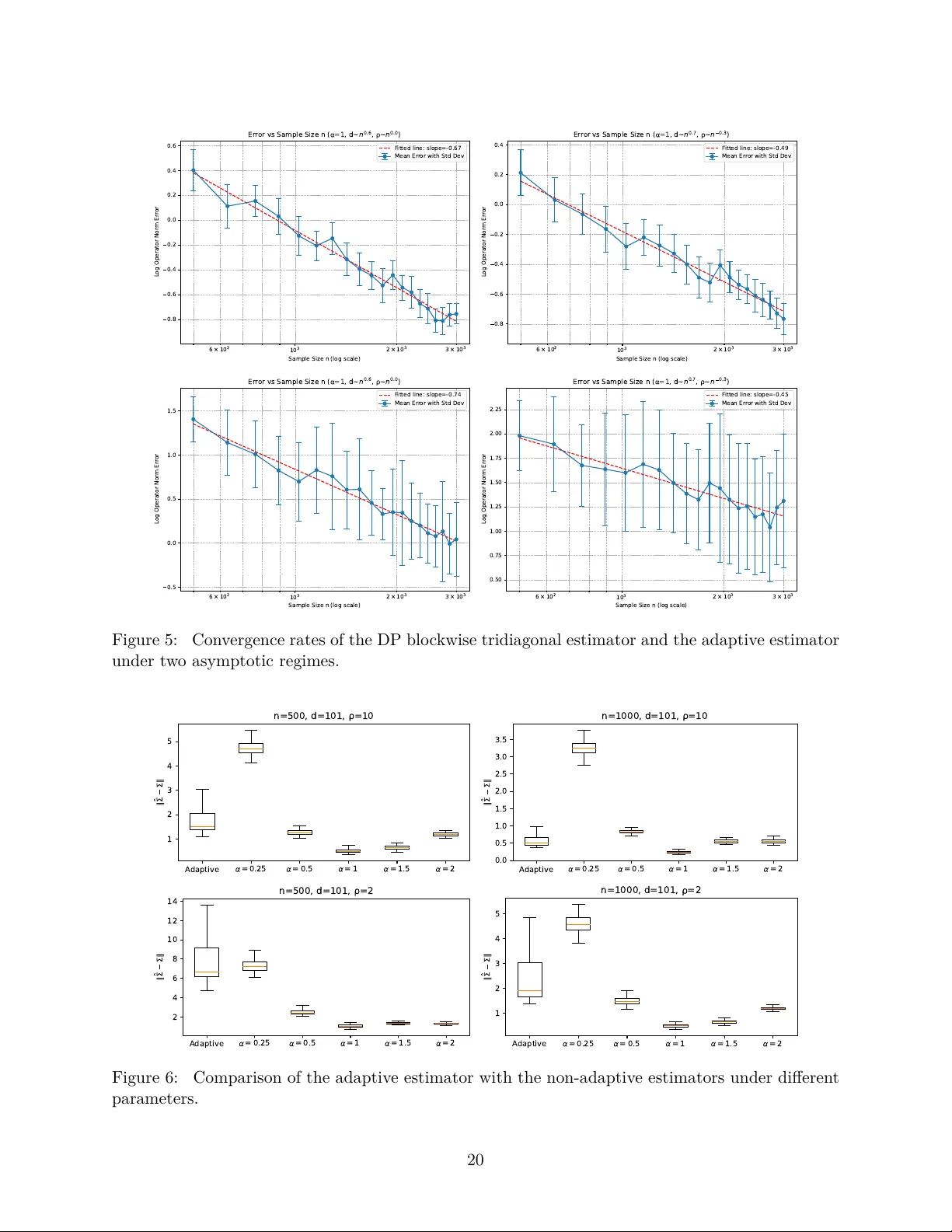
Minimax and A daptiv e Co v ariance Matrix Estimation under Diﬀeren tial Priv acy T. T on y Cai Departmen t of Statistics and Data Science The Wharton Sc ho ol, Univ ersity of P ennsylv ania tcai@wharton.upenn.edu Yic heng Li Departmen t of Statistics and Data Science T singh ua Univ ersity liyc22@mails.tsinghua.edu.cn Abstract The cov ariance matrix pla ys a fundamen tal role in the analysis of high-dimensional data. This paper studies minimax and adaptive estimation of high-dimensional bandable co v ariance matrices under diﬀeren tial priv acy constraints. W e prop ose a no vel diﬀeren tially priv ate block- wise tridiagonal estimator that ac hieves minimax-optimal con vergence rates under both the op- erator norm and the F rob enius norm. In contrast to the non-priv ate setting, the priv acy-induced error exhibits a polynomial dep endence on the ambien t dimension, revealing a substantial ad- ditional cost of priv acy . T o establish optimalit y , w e develop a new diﬀeren tially priv ate v an T rees inequalit y and construct carefully designed prior distributions to obtain matching minimax low er bounds. The prop osed priv ate v an T rees inequality applies more broadly to general priv ate estimation prob- lems and is of independent interest. W e further in tro duce an adaptive estimator that attains the optimal rate up to a logarithmic factor without prior knowledge of the deca y parameter, based on a no vel hierarc hical tridiagonal approac h. Numerical experiments corrob orate the theoretical results and illustrate the fundamen tal priv acy-accuracy trade-oﬀ. Keyw ords: Adaptiv e estimation, Cov ariance matrix, Diﬀerential priv acy , Minimax rate of conv er- gence Con ten ts 1 In tro duction 3 1.1 Main Contribution . . . . . . . . . . . . . . . . . . . . . . . . . . . . . . . . . . . . . 4 1.2 Related W ork . . . . . . . . . . . . . . . . . . . . . . . . . . . . . . . . . . . . . . . . 5 1.3 Organization . . . . . . . . . . . . . . . . . . . . . . . . . . . . . . . . . . . . . . . . 6 1.4 Notations and Assumptions . . . . . . . . . . . . . . . . . . . . . . . . . . . . . . . . 6 2 Co v ariance Estimation under DP 6 2.1 Mec hanism for DP . . . . . . . . . . . . . . . . . . . . . . . . . . . . . . . . . . . . . 7 2.2 Blo c kwise T ridiagonal Estimator . . . . . . . . . . . . . . . . . . . . . . . . . . . . . 7 2.3 Estimation Error under Op erator Norm . . . . . . . . . . . . . . . . . . . . . . . . . 8 2.4 Estimation Error under F rob enius Norm . . . . . . . . . . . . . . . . . . . . . . . . . 9 1 2.5 Discussions . . . . . . . . . . . . . . . . . . . . . . . . . . . . . . . . . . . . . . . . . 10 2.6 Pro of Idea . . . . . . . . . . . . . . . . . . . . . . . . . . . . . . . . . . . . . . . . . . 11 3 Minimax Lo w er Bound under Diﬀerential Priv acy 12 3.1 A DP v an T rees Inequality . . . . . . . . . . . . . . . . . . . . . . . . . . . . . . . . 12 3.2 Minimax Low er Bounds for Co v ariance Estimation . . . . . . . . . . . . . . . . . . . 13 4 A daptiv e Estimator 15 4.1 Construction of the Estimator . . . . . . . . . . . . . . . . . . . . . . . . . . . . . . . 15 4.2 Theoretical Guarantees . . . . . . . . . . . . . . . . . . . . . . . . . . . . . . . . . . 16 4.3 Pro of Idea . . . . . . . . . . . . . . . . . . . . . . . . . . . . . . . . . . . . . . . . . . 17 5 Numeric Exp erimen ts 18 6 Estimating the Precision Matrix under DP 21 7 Discussion 21 A Proofs for Section 2 22 A.1 Priv acy Guarantee . . . . . . . . . . . . . . . . . . . . . . . . . . . . . . . . . . . . . 22 A.2 Concen trations . . . . . . . . . . . . . . . . . . . . . . . . . . . . . . . . . . . . . . . 23 A.3 Blocking Lemma . . . . . . . . . . . . . . . . . . . . . . . . . . . . . . . . . . . . . . 26 A.4 Pro of of Theorem 2.7 . . . . . . . . . . . . . . . . . . . . . . . . . . . . . . . . . . . . 27 A.5 Pro of of Theorem 2.5 . . . . . . . . . . . . . . . . . . . . . . . . . . . . . . . . . . . . 27 B Pro ofs for the A daptiv e Estimator 29 B.1 Pro of of Theorem 4.2 . . . . . . . . . . . . . . . . . . . . . . . . . . . . . . . . . . . . 30 B.2 Pro of of Theorem 4.3 . . . . . . . . . . . . . . . . . . . . . . . . . . . . . . . . . . . . 32 C V an T rees Inequality for Diﬀeren tial Priv acy 33 D Pro of of the Minimax Lo w er Bounds 36 D.1 F rob enius Norm, Pro of of Theorem 3.3 . . . . . . . . . . . . . . . . . . . . . . . . . . 36 D.2 Schatten Norm, Pro of of Theorem 3.2 . . . . . . . . . . . . . . . . . . . . . . . . . . 37 D.3 Prior Distribution o ver Op erator Norm Ball: Pro of of Lemma 3.5 . . . . . . . . . . . 38 E Pro ofs Related to Estimating the Precision Matrix 41 E.1 Upp er Bounds . . . . . . . . . . . . . . . . . . . . . . . . . . . . . . . . . . . . . . . 41 E.2 Minimax Low er Bounds . . . . . . . . . . . . . . . . . . . . . . . . . . . . . . . . . . 41 F Auxiliary Results 42 F.1 Div ergence . . . . . . . . . . . . . . . . . . . . . . . . . . . . . . . . . . . . . . . . . 42 F.2 Concen tration Inequalities . . . . . . . . . . . . . . . . . . . . . . . . . . . . . . . . . 42 F.3 T runcation . . . . . . . . . . . . . . . . . . . . . . . . . . . . . . . . . . . . . . . . . 43 F.4 Fisher Information of Normal Distributions . . . . . . . . . . . . . . . . . . . . . . . 44 2 1 In tro duction The cov ariance matrix pla ys a cen tral role in the analysis of high-dimensional data. Bey ond its in trinsic imp ortance in man y scientiﬁc and engineering applications, cov ariance structure underlies a wide range of fundamental statistical metho ds, including principal comp onen t analysis, discriminan t analysis, clustering, and regression. Accurate estimation of the cov ariance matrix is therefore a cornerstone of multiv ariate analysis. Supp ose we observe indep enden t and identically distributed random v ectors x 1 , . . . , x n ∈ R d with p opulation co v ariance matrix Σ . Classical estimators of Σ such as the sample cov ariance matrix p erform well when the dimension d is small relative to the sample size n . Ho wev er, mo dern datasets often operate in the high-dimensional regime where d is comparable to or even muc h larger than n . In this setting, the sample co v ariance matrix b ecomes unstable or singular, motiv ating the dev elopment of structural assumptions and regularized estimators for high-dimensional co v ariance matrices; see Cai et al. [ 17 ] for a comprehensive review. A widely studied structural assumption is that of b andable cov ariance matrices, where oﬀ- diagonal entries decay as they mov e a wa y from the diagonal. Suc h matrices arise naturally in temp oral, spatial, and other ordered data settings, reﬂecting the weak ening of correlations with increasing separation. Bandable co v ariance matrices capture this phenomenon while remaining mathematically tractable. Optimal rates and adaptiv e procedures for estimating bandable co- v ariance matrices in the non-priv ate setting ha ve b een established under b oth the op erator and F rob enius norms. In particular, Cai et al. [ 15 ] derived the minimax rate of con vergence under the op erator norm and proposed an optimal-rate tap ering estimator. Later, Cai and Y uan [ 13 ] in tro duced a blo c k thresholding estimator that adaptively attains the optimal rate ov er a collection of parameter spaces without requiring kno wledge of the deca y parameter. See Cai et al. [ 17 ] for a detailed survey of these results. A t the same time, many datasets used for co v ariance estimation contain sensitive information, raising signiﬁcan t priv acy concerns. Improp er disclosure can lead to harms suc h as iden tity theft, discrimination, or loss of trust. These risks are particularly acute in domains lik e healthcare, where genetic and medical records enable imp ortant scientiﬁc adv ances but are highly sensitive [ 2 , 31 ]. Such concerns underscore the need for metho ds that enable reliable statistical inference while provi ding strong protections for individual priv acy . Among the approaches prop osed to address this challenge, diﬀerential priv acy (DP) [ 27 , 29 ] has emerged as a leading and mathematically rigorous framework for priv acy-preserving data analysis. DP provides guarantees that the inclusion or exclusion of any single individual’s data has only a limited eﬀect on the outcome of an analysis, thereby protecting against inference attac ks even in the presence of auxiliary information. F ormally , a randomized algorithm M satisﬁes ( ϵ, δ ) -DP if, for any adjacent datasets S, S ′ ∈ D (diﬀering by one element) and measurable output sets A , P { M ( S ) ∈ A } ≤ e ϵ P  M ( S ′ ) ∈ A  + δ. While ( ϵ, δ ) -DP is widely adopted, the zero-concentrated diﬀerential priv acy (zCDP) framew ork [ 11 , 28 ], based on Rén yi div ergences, provides tighter comp osition guaran tees for complex algorithms through a single priv acy parameter ρ > 0 . Recall that the α -Rényi div ergence b etw een t wo random v ariables X and Y , ass ociated with probability measures P and Q , is deﬁned as D α ( X ∥ Y ) = 1 α − 1 log E  d P d Q ( X )  α , α > 1 . The deﬁnition of ρ -zCDP is giv en b elo w. 3 Deﬁnition 1.1 ( ρ -zCDP) . A randomized algorithm M : D → A satisﬁes ρ -zero-concentrated DP ( ρ -zCDP) if for all adjacent S, S ′ ∈ D , D α ( M ( S ) ∥ M ( S ′ )) ≤ ρα, ∀ α ∈ (1 , ∞ ) , (1.1) where D α ( X ∥ Y ) is taken only o ver the randomness of M conditioned on the data. The connection b et ween ρ -zCDP and ( ϵ, δ ) -DP is well-established in the literature, as is illus- trated in the following lemma [ 11 , 27 ]. Lemma 1.2. If M is ( ϵ, 0) -DP, then M is ( ϵ 2 / 2) -zCDP. Conversely, If M is ρ -zCDP, then M is  ρ + 2 p ρ log(1 /δ ) , δ  -DP for every δ ∈ (0 , 1) . In p articular, for ϵ ∈ (0 , 1] and δ ∈ (0 , e − 1 ] , ρ -zCDP with ρ ≤ ϵ 2 (8 log(1 /δ )) − 1 implies ( ϵ, δ ) -DP. Although ( ϵ, δ ) -DP remains the most commonly used framework, ρ -zCDP oﬀers several adv an- tages for precise analysis and the design of complex algorithms. In particular, its div ergence-based form ulation and single-parameter characterization of the priv acy budget often simplify comp osi- tion analyses and lead to tighter guaran tees. F or this reason, w e adopt ρ -zCDP as the primary priv acy notion in this paper; the corresp onding ( ϵ, δ ) -DP guarantees can b e readily derived from the relationship describ ed ab o v e. T o achiev e diﬀeren tial priv acy , a common approach is to add appropriately calibrated noise to the output of a non-priv ate algorithm. While it is easy to ensure priv acy b y adding large amoun ts of noise, excessiv e noise can substantially degrade statistical accuracy . A cen tral challenge in diﬀerentially priv ate statistics is therefore to balance priv acy protection with statistical utility , a trade-oﬀ often referred to as the “cost of priv acy” [ 18 ]. The optimal priv acy–utilit y trade-oﬀ dep ends on the underlying statistical problem, with results established for settings such as mean estimation [ 6 , 32 ], linear regression [ 18 ], and nonparametric regression [ 19 ], among others. Understanding this trade-oﬀ is essen tial for designing DP algorithms that pro vide rigorous priv acy guarantees while preserving statistical eﬃciency . Recen t work on diﬀerentially priv ate cov ariance estimation has largely fo cused on unstructured co v ariance matrices. In this setting, a direct application of the well-kno wn Gaussian mechanism to the sample co v ariance matrix ac hieves optimal rates [ 4 , 24 , 36 , 38 ]. In particular, under mild conditions the minimax risk under zCDP satisﬁes inf ˆ Σ ∈M ρ sup Σ E    ˆ Σ DP − Σ    2 ≍ d n + d 3 ρn 2 , (1.2) where M ρ denotes the class of all ρ -zCDP estimators. Analogous results hold under the F rob enius norm. Ho wev er, as in the non-priv ate setting, this naive estimator do es not exploit structural assumptions (such as bandable co v ariance structure) and is sub optimal when such structure is presen t, particularly in high dimensions. Developing DP co v ariance estimators that eﬀectively incorp orate structural assumptions remains an imp ortan t op en problem. 1.1 Main Contribution In this pap er, we study the problem of estimating bandable co v ariance matrices under diﬀerential priv acy constrain ts. First, w e prop ose a nov el DP blo c kwise tridiagonal estimator that achiev es the minimax optimal rate inf ˆ Σ ∈M ρ sup Σ ∈F α E    ˆ Σ − Σ    2 ≍ n − 2 α 2 α +1 +  d ρn 2  α α +1 , 4 where F α denotes the class of bandable cov ariance matrices with deca y parameter α > 0 (see ( 2.2 )) and M ρ denotes the class of all ρ -zCDP estimators. Notably , this rate is ac hieved without an y logarithmic loss in n , d , or ρ , whereas logarithmic factors commonly appear in many DP estimation problems [ 4 , 18 , 20 , 24 ]. The estimator is constructed b y partitioning the sample cov ariance matrix in to blo c ks, retaining only tridiagonal blo c ks, and adding carefully calibrated Gaussian noise to ensure priv acy . The optimal blo ck size is c hosen to balance the bias, statistical v ariance, and priv acy-induced v ariance. W e also establish minimax optimal rates under the F rob enius norm, whic h diﬀer from those under the op erator norm. Our results reveal a p olynomial dep endence on the dimension d in the cost of priv acy even under bandable structure, in con trast to the logarithmic dep endence typically seen in non-priv ate statistical error terms, highlighting the intrinsic diﬃcult y of priv ate estimation in high dimensions. Second, w e develop a no vel DP v an T rees inequality that pro vides a general tool for deriving minimax low er b ounds under DP constraints. Using this inequality , w e construct explicit prior distributions to obtain minimax low er bounds for bandable cov ariance estimation that match our upp er bounds under b oth the op erator and F rob enius norms. The inequalit y is established through a new connection b et ween Fisher information and the ρ -zCDP constraint. Moreo ver , lev eraging the ρ -zCDP formulation yields sharp low er b ounds without the log (1 /δ ) losses that frequently arise in ( ϵ, δ ) -DP analyses. Due to its conceptual simplicit y and broad applicabilit y , the DP v an T rees inequalit y may b e useful for establishing lo wer b ounds in other priv ate estimation problems. Third, we prop ose an adaptiv e estimator that achiev es optimal rates (up to log n factors) with- out requiring prior kno wledge of the decay parameter α , extending adaptivity results from the non-priv ate setting [ 13 ] to the DP framework. The estimator employs a nov el hierarchical tridi- agonal structure that simpliﬁes b oth the construction and analysis compared with previous blo ck- thresholding approac hes [ 13 ]. The proof of adaptivity relies on a reﬁned allo cation of priv acy budgets and fully exploits the hierarc hical structure to con trol b oth statistical and priv acy errors across multiple scales. Finally , we conduct numerical exp erimen ts to v alidate the theoretical results. The simulations conﬁrm the eﬀectiv eness of the prop osed estimators and illustrate the impact of priv acy constraints on estimation accuracy . They also demonstrate the adv an tage of the adaptive estimator when the deca y parameter α is unknown. 1.2 Related W ork Recen t w ork on diﬀerentially priv ate cov ariance estimation has primarily fo cused on unstructured co v ariance matrices. Baseline approac hes typically add Laplace or Gaussian noise to the sample co v ariance matrix [ 27 , 30 ]. Subsequen t dev elopments include (i) metho ds for Gaussian data that target the Mahalanobis loss ∥ Σ − 1 2 ( ˆ Σ − Σ)Σ − 1 2 ∥ F in ill-conditioned settings [ 3 , 5 , 10 , 34 ], (ii) robust co v ariance estimation under general distributions [ 24 , 35 ], and (iii) optimal priv ate estimation for spiked cov ariance mo dels [ 20 ]. Ho wev er, none of these works consider structured cov ariance matrices, suc h as bandable co v ariance structures. In contrast, there is a rich literature on structured cov ariance estimation in the non-priv ate setting. F or bandable co v ariance matrices, regularization metho ds including banding [ 9 ], tap er- ing [ 15 ], thresholding [ 8 ], and adaptive blo c k-thresholding [ 13 ] ha ve b een prop osed to exploit the structural decay of correlations. Optimal rates of con vergence under b oth op erator and F rob enius norms hav e b een established [ 15 ]. Other commonly studied structures include sparse cov ariance matrices [ 14 , 22 ], T o eplitz cov ariance structures [ 16 ], and sparse precision matrices [ 23 ]. See Cai et al. [ 17 ] for a comprehensiv e ov erview of this literature. Priv acy constraints typically introduce an additional “cost of priv acy” in minimax rates. V ar- 5 ious tec hniques ha v e been dev elop ed to derive low er bounds under diﬀeren tial priv acy , includ- ing adaptations of classical information-theoretic to ols such as F ano’s inequality and Le Cam’s metho d [ 1 , 25 , 26 ], ﬁngerprinting co des and score attacks [ 7 , 18 , 21 , 33 , 37 ], and v an T rees–type inequalities [ 19 , 41 ]. More recently , Naray anan [ 36 ], P ortella and Harvey [ 38 ] established minimax lo wer b ounds for estimating general unstructured cov ariance matrices under DP using Wishart distributions. Ho wev er, man y existing lo w er b ound techniques are tec hnically in volv ed and often problem-sp eciﬁc. Moreo v er, they primarily fo cus on the ( ϵ, δ ) -DP framew ork and typically incur additional log(1 /δ ) factors. In con trast, our v an T rees inequalit y under the ρ -zCDP framework pro- vides a simpler and more general approach for deriving lo wer b ounds and av oids such logarithmic losses. 1.3 Organization The rest of the pap er is organized as follo ws. Section 2 introduces the blo c kwise tridiagonal es- timator and establishes the corresp onding upp er b ounds. Section 3 p resen ts the DP v an T rees inequalit y and derives minimax lo wer b ounds for bandable cov ariance matrix estimation under DP . In Section 4 , we dev elop the adaptiv e estimator and analyze its p erformance. Numerical results are rep orted in Section 5 . Section 6 considers extensions of our metho dology to precision ma- trix estimation and Section 7 concludes with a discussion of our ﬁndings and directions for future researc h. 1.4 Notations and Assumptions W e use C and c to denote generic p ositiv e constants that may v ary from line to line. W rite a ≲ b if there exists a constant C > 0 suc h that a ≤ C b , and write a ≍ b if a ≲ b and b ≲ a . W e use the notations a ∧ b and a ∨ b to denote min( a, b ) and max ( a, b ) , resp ectiv ely . The indicator function is denoted by 1 {·} , and | S | denotes the cardinality of a set S . W e write [ d ] = { 1 , 2 , . . . , d } . F or a matrix A , ∥ A ∥ denotes the s pectral (op erator) norm and ∥ A ∥ F the F rob enius norm. W e write ⟨ A, B ⟩ = T r( A ⊤ B ) for the trace inner pro duct. The matrix ℓ r norm is deﬁned as ∥ A ∥ ℓ r = max ∥ x ∥ ℓ r =1 ∥ Ax ∥ ℓ r . In particular, ∥ A ∥ ℓ 2 = ∥ A ∥ is the sp ectral norm, ∥ A ∥ ℓ ∞ = max i P j | A ij | is the maxim um absolute row sum, and ∥ A ∥ ℓ 1 = max j P i | A ij | is the maximum absolute column sum. The matrix Sc hatten- q norm is deﬁned as ∥ A ∥ S q = ( P i σ i ( A ) q ) 1 /q , where σ i ( A ) are the singular v alues of A . In particular, ∥ A ∥ S 2 = ∥ A ∥ F is the F rob enius norm and ∥ A ∥ S ∞ = ∥ A ∥ is the sp ectral norm. F or a matrix M ∈ R d × d and an index set B ⊆ [ d ] 2 , we denote by M B or M [ B ] the matrix obtained by setting all entries outside B to zero. A similar notation v I applies to vectors. W e call B a blo ck if B = I × J for some I , J ⊆ [ d ] , and sa y that it has size k if | I | = | J | = k . The sub-Gaussian norm [ 40 ] for a random v ariable ξ is deﬁned as ∥ ξ ∥ ψ 2 = inf { t > 0 : E ( e ξ 2 /t 2 ) ≤ 2 } , and for a random v ector X as ∥ X ∥ ψ 2 : = sup v : ∥ v ∥ 2 =1 ∥⟨ X , v ⟩∥ ψ 2 . 2 Co v ariance Estimation under DP In this section, w e introduce our blo c kwise tridiagonal DP estimator for bandable cov ariance ma- trices and establish minimax upp er b ounds under b oth the op erator and F rob enius norms. The blo c kwise tridiagonal structure plays a k ey role: it facilitates b oth the calibration of priv acy noise and the subsequent statistical analysis. Throughout the paper, we assume that the i.i.d. samples are sub-Gaussian random vectors satisfying ∥ x i ∥ ψ 2 ≤ K for some constant K > 0 . W e further assume, without loss of generality , 6 that d ≲ n γ for some ﬁxed constant γ > 0 ; otherwise, as will b e shown in the follo wing sections, the minimax risk under priv acy constraints would diverge. 2.1 Mec hanism for DP W e brieﬂy review the fundamen tal tools in diﬀerential priv acy that are widely used in the literature. T o achiev e diﬀerential priv acy , a standard approac h is to add appropriately calibrated noise to the output of a non-priv ate algorithm with b ounded sensitivit y . The comp osition prop erties of DP mec hanisms are also essen tial for analyzing algorithms that in volv e m ultiple steps or iterativ e pro cedures. In particular, for ρ -zCDP , w e hav e the following Gaussian mec hanism and comp osition lemmas [ 11 , 27 ]. Lemma 2.1 (Gaussian Mechanism) . L et f : D → R p b e an algorithm such that sup D,D ′ adjac ent   f ( D ) − f ( D ′ )   2 ≤ ∆ . Then, the algorithm M f ( D ) = f ( D ) + σ w is ρ -zCDP, wher e w ∼ N (0 , I p ) and σ 2 = ∆ 2 2 ρ . Lemma 2.2 (Comp osition) . If M : D → Y is ρ -zCDP and f : Y → Z is an arbitr ary algorithm, then f ◦ M is also ρ -zCDP. If M 1 , . . . , M T ar e ρ 1 , . . . , ρ T -zCDP and M is a function of M 1 , . . . , M T , then M is ρ -zCDP for ρ = P t ρ t . 2.2 Blo c kwise T ridiagonal Estimator Before introducing the estimator, we ﬁrst deﬁne several auxiliary notations. Let k > 0 denote the blo c k size and let N k = ⌈ d/k ⌉ b e the num b er of blo c ks. Deﬁne I k,l = [1 + ( l − 1) k , lk ] ∩ { 1 , . . . , d } , l ∈ [ N k ] , and introduce the blo c ks B k ; l ,l ′ = I k,l × I k,l ′ , B k ; l = B k ; l ,l , B k ; l + = B k ; l ,l +1 , B k ; l − = B k ; l ,l − 1 . (2.1) As a building blo c k of our pro cedure, Algorithm 1 describ es ho w to compute a diﬀeren tially priv ate estimate for a single blo ck of the cov ariance matrix. Algorithm 1 DP Co v ariance Blo c k: DPCovBlo ck ( X , B ; ρ 0 , L ) Input: Data X = ( x 1 , . . . , x n ) with x 1 , . . . , x n ∈ R d , blo c k B = I × J , priv acy parameter ρ 0 , truncation leve l L . Let ˜ x i,I = x i,I 1 n ∥ x i,I ∥ 2 ≤ L | I | o and ˜ x i,J = x i,J 1 n ∥ x i,J ∥ 2 ≤ L | J | o . Let ˆ µ I = 1 n P i ∈ [ n ] ˜ x i,I and ˆ µ J = 1 n P i ∈ [ n ] ˜ x i,J . Let ˜ Σ B = 1 n P i ∈ [ n ] ˜ x i,I ˜ x ⊤ i,J − ˆ µ I ˆ µ ⊤ J , return ˆ Σ DP B = ˜ Σ B + σ M M B , where M B = GUE( d ) B and σ 2 M = 18 L 2 | B | ρ 0 n 2 . Prop osition 2.3. A lgorithm 1 is ρ 0 -zCDP. By combining the abov e building blo c ks, w e deﬁne our blo c kwise tridiagonal estimator in Al- gorithm 2 . 7 Algorithm 2 DP Blo c kwise T ridiagonal Estimator Input: Data x 1 , . . . , x n ∈ R d , blo c k size k , priv acy parameter ρ , truncation level L . Output: ρ -zCDP estimator ˆ Σ DP . T ak e ρ 0 = ρ/ (2 N k ) . Compute ˆ Σ DP B k ; l = DPCovBlo ck ( X, B k ; l ; ρ 0 , L ) and ˆ Σ DP B k ; l + = DPCovBlo ck ( X, B k ; l + ; ρ 0 , L ) for all l ∈ [ N k ] . Fill the low er triangular part by symmetry , leaving other entries to zero. return ˆ Σ DP . Figure 1: Illustration of the blo c kwise tridiagonal estimator The estimator retains only the main diagonal blo c ks and the ﬁrst super- and sub-diagonal blo c ks of the cov ariance matrix, while setting all other entries to zero; see Figure 1 for an illustration. The blo c k size parameter k will b e chosen later to balance the bias–v ariance–priv acy trade-oﬀ. Compared with the tap ering estimator of Cai et al. [ 15 ], the prop osed blo c kwise tridiagonal construction is simpler and b etter suited for the priv ate setting, as it streamlines b oth the calibration of priv acy noise and the subsequent statistical analysis. Moreo ver, b ecause the estimator focuses only on a limited subset of cov ariance en tries, the amoun t of noise required to guarantee priv acy is substantially reduced, enabling optimal estimation accuracy under priv acy constraints. Finally , b y inv oking the comp osition prop ert y in Lemma 2.2 , w e ensure that the o verall estimator satisﬁes ρ -zCDP . Prop osition 2.4. A lgorithm 2 is ρ -zCDP. 2.3 Estimation Error under Op erator Norm Let us deriv e the rates of con vergence for the blockwise tridiagonal estimator under the operator norm. T o this end, consider the follo wing class of bandable co v ariance matrices: F α =  Σ : ∀ k -oﬀ-diagonal blo c k R k , ∥ Σ R k ∥ ≤ C 1 k − α and ∥ Σ ∥ ≤ C 2  , (2.2) where C 1 , C 2 > 0 are constants. Here, a k -oﬀ-diagonal block means a blo c k lying ab o v e the k -th sup er-diagonal (or symmetrically b elo w the k -th sub-diagonal), e.g. a region con tained in 8 { ( i, j ) : j ≥ i + k } . An example of such a blo c k is [1 , . . . , i 0 ] × [ i 0 + k , . . . , d ] for some i 0 . This condition enforces a p o wer-la w deca y of the co v ariance as entries mov e a wa y from the main diagonal. Alternativ ely , th e class can b e describ ed in terms of the op erator norm of co v ariances b et ween t wo k -separated index sets I , J ⊆ [ d ] , i.e. min i ∈ I ,j ∈ J | i − j | ≥ k : sup k -separated I ,J ∥ Co v( x I , x J ) ∥ ≤ C 1 k − α . F rom this p erspective, the class F α captures the deca y of long-range dep endencies in the random v ector x . Th us, it is a natural mo del for v arious applications where suc h decay o ccurs, e.g., time series analysis and spatial statistics. Another closely related class controls the tail sum of each row [ 13 , 15 ]: G α =    Σ : max i X j : | i − j | >k | Σ ij | ≤ C 1 k − α and ∥ Σ ∥ ≤ C 2    . (2.3) Using the fact ∥ A ∥ 2 ≤ ∥ A ∥ ℓ 1 ∥ A ∥ ℓ ∞ , it is easy to see that F α ⊇ G α , namely F α is a larger class. Nev ertheless, we will see in the following that the same upp er b ound holds under the larger class F α . Hence, w e will fo cus on the broader class F α for op erator norm throughout this pap er. Theorem 2.5. L et Σ ∈ F α for some α > 0 . Consider the blo ckwise tridiagonal estimator ˆ Σ DP given in A lgorithm 2 with blo ck size k ≤ cn for some smal l c onstant c > 0 . Then, we have E    ˆ Σ DP − Σ    2 ≲ k + log d n + dk ( k + log d ) ρn 2 + k − 2 α . (2.4) Theorem 2.5 characterizes the estimation error under op erator norm with arbitrary blo c k size k . Optimizing ov er k yields the follo wing corollary . Corollary 2.6. Under the same setting as in The or em 2.5 , supp ose that ρn 2 /d ≳ (log d ) 2( α +1) . T ake k ≍ min( n 1 / (2 α +1) , ( ρn 2 /d ) 1 / (2 α +2) ) ∨ log d. (2.5) Then, we have E    ˆ Σ DP − Σ    2 ≲ n − 2 α 2 α +1 +  d ρn 2  α α +1 (2.6) 2.4 Estimation Error under F robenius Norm Regarding the F rob enius norm, as in Cai and Y uan [ 13 ], the following class of bandable cov ariance matrices will b e considered: H α = n Σ : | Σ ij | ≤ C 1 | i − j | − ( α +1) and ∥ Σ ∥ ≤ C 2 o , (2.7) where C 1 , C 2 are positive constants. This class imp oses a stronger deca y condition on each indi- vidual cov ariance entry as they mo ve aw a y from the main diagonal. W e note that H α ⊆ G α ⊆ F α , th us H α is the smallest class among the three. Theorem 2.7. L et Σ ∈ H α for some α > 0 . Consider the blo ckwise tridiagonal estimator ˆ Σ DP given in A lgorithm 2 with blo ck size k ≤ cn for some smal l c onstant c > 0 . W e have 1 d E    ˆ Σ DP − Σ    2 F ≲ k n + dk 2 ρn 2 + k − (2 α +1) . (2.8) 9 Corollary 2.8. Under the same setting as in The or em 2.7 , take k = min( n 1 / (2( α +1)) , ( ρn 2 /d ) 1 / (2 α +3) ) . (2.9) Then, we have 1 d E    ˆ Σ DP − Σ    2 F ≲ n − 2 α +1 2( α +1) +  d ρn 2  2 α +1 2 α +3 . (2.10) 2.5 Discussions Let us discuss some implications of the ab o ve results. 2.5.1 Minimax Optimal Rates Com bining the upp er b ounds in Corollary 2.6 and Corollary 2.8 with the minimax low er b ounds in Theorem 3.2 and Theorem 3.3 established in the next section, we see that the blockwise tridiagonal estimator ac hieves the minimax optimal rates under b oth operator norm and F rob enius norm when the blo c k size k is prop erly chosen. T o b e more precise, let us focus on the op erator norm and consider the case when d ≳ n 1 / (2 α +1) ∨ ( ρn 2 ) 1 / (2 α +3) . Otherwise, the naiv e priv atized empirical co v ariance estimator achiev es the minimax rate as shown in ( 1.2 ). In this case, as long as ρn 2 /d ≳ (log d ) 2( α +1) , the blo c kwise tridiagonal estimator with prop erly chosen blo c k size k ac hieves the minimax optimal rate in ( 2.6 ). The ﬁrst term in the rate corresp onds to the non-priv ate minimax rate [ 15 ] under the slightly larger class F α , while the second term c haracterizes the additional cost due to priv acy constraints. When ρ ≲ dn − 2 α 2 α +1 , the priv acy cost dominates the minimax rate, otherwise the statistical error dom- inates. This kind of statistics-priv acy error trade-oﬀ is commonly observed in priv ate estimation problems [ 18 – 20 ]. Additionally , w e note that the requirement ρn 2 /d ≳ (log d ) 2( α +1) is mild, as otherwise the lo wer b ounds sho w that the minimax rates would only decrease logarithmically with n . W e also emphasize that no loss of m ultiplicative logarithmic factors o ccurs b et ween the upp er and low er b ounds under ρ -zCDP. In comparison, for man y other DP estimation problems (e.g., Bisw as et al. [ 10 ], Cai et al. [ 18 , 20 , 21 ]), particularly those under ( ϵ, δ ) -DP constrain ts, a gap with resp ect to logarithmic factors suc h as log n or log(1 /δ ) often exists b et ween the upp er and low er b ounds. Conv erting ρ -zCDP to ( ϵ, δ ) -DP using Lemma 1.2 , we can state our upp er b ounds under ( ϵ, δ ) -DP constrain ts, with a cost of additional log(1 /δ ) factors. Finally , we remark that if there is no priv acy constraint, i.e., ρ = ∞ , the blo c kwise tridiagonal estimator with k ≍ n 1 / (2 α +1) reco vers the optimal non-priv ate rate in Cai et al. [ 15 ], so the blo c kwise tridiagonal estimator itself is also a new optimal estimator in the non-priv ate setting. 2.5.2 Block Size P arameter The blo c k size k is a crucial tuning parameter that balances the bias–v ariance–priv acy trade-oﬀ, as reﬂected in the three terms in the upp er b ounds ( 2.4 ) and ( 2.8 ). In the non-priv ate setting, k corresp onds to the bandwidth parameter in the tap ering estimator in Cai et al. [ 15 ]: increasing k reduces the bias since more co v ariance entries are estimated. Ho wev er, in the priv ate setting, increasing k also increases the v ariance due to the additional noise added for priv acy . Th us, the op- timal choice of k balances these three asp ects: the critical v alue corresp onding to the bias–v ariance trade-oﬀ is k ≍ n 1 / (2 α +1) as in the non-priv ate case [ 15 ], while the critical v alue corresp onding to the bias–priv acy trade-oﬀ is k ≍ ( ρn 2 /d ) 1 / (2 α +2) . Balancing these t wo yields the optimal blo c k 10 size choice. This phenomenon of bias–v ariance–priv acy trade-oﬀ is commonly observed in priv ate estimation problems [ 18 – 20 ]. 2.5.3 Dimension-Dependent Cost of Priv acy F rom the minimax rates, w e see that the substantial dimensional dependence under DP constraints is inevitable. In the non-priv ate setting [ 15 ], the minimax rate under op erator norm only dep ends on the dimension d logarithmically through an additive term log d n (whic h is omitted in our results as- suming d ≲ n γ ). In sharp con trast, under DP constrain ts, the cost of priv acy term  d/ ( ρn 2 )  α/ ( α +1) dep ends on d p olynomially . In particular, even when the priv acy budget ρ is constan tly large, a minimal requirement of d ≲ n 2 is needed to ensure consistency . This result suggests the imp ossi- bilit y of accurate priv ate estimation in very high-dimensional problems, ev en when the underlying structure is present. 2.5.4 Operator Norm vs. F rob enius Norm As shown in Corollary 2.6 and Corollary 2.8 , the optimal choice of the blo c k size and conv ergence rates under F rob enius norm and operator norm are diﬀerent, similar to the non-priv ate setting [ 15 ]: the optimal pro cedure under op erator norm is not optimal under F rob enius norm, and vice v ersa. This phenomenon is due to the diﬀerent wa ys these t wo norms aggregate the estimation errors across diﬀerent matrix en tries. Therefore, it is essen tial to sp ecify the norm of interest for the optimal tuning of the blo ck size. 2.5.5 Exponential Deca y Co v ariance Class Our results can b e easily extended to co v ariance classes with exp onen tial decay . If the cov ariance en tries decay exp onen tially aw ay from the diagonal, i.e., we hav e ∥ Σ R k ∥ ≤ C 1 exp( − γ k ) . Then, it can b e shown that b y taking k ≍ (log n ) ∧ (log( ρn 2 /d )) , E    ˆ Σ DP − Σ    2 ≲ log n n + d ρn 2 " log ρn 2 d ! + log d # 2 . 2.5.6 Estimation Error under Sc hatten Norm The upp er b ound in operator norm can b e directly extended to Schatten- q norm for q ≥ 2 . Using the fact that for an y matrix A ∈ R d × d , ∥ A ∥ S q ≤ d 2 q ∥ A ∥ 2 the follo wing corollary is immediate (when ρn 2 /d ≳ (log d ) 2( α +1) ): sup Σ ∈F α d − 2 q E    ˆ Σ DP − Σ    2 S q ≲ n − 2 α 2 α +1 +  d ρn 2  α α +1 . In fact, we can also show that this rate is minimax optimal; see the discussion after Theorem 3.2 . 2.6 Pro of Idea F acilitated b y the tridiagonal block structure, the pro ofs of Theorem 2.5 and Theorem 2.7 are considerably simpler than those for the tap ering estimator in Cai et al. [ 15 ]. W e ﬁrst analyze the error for each individual blo c k computed in Algorithm 1 , and then combine them to b ound the ov erall error. The error for eac h blo c k can b e decomposed in to three parts: the bias due to 11 truncation, the v ariance due to ﬁnite samples, and the additional v ariance due to the noise added for priv acy . T o control the ov erall error, we lev erage the tridiagonal structure to sho w that the o verall op erator norm error can b e b ounded b y    ˆ Σ DP − Σ    ≤ 4 max B    ˆ Σ DP B − Σ B    , where the maximum is taken o ver all the tridiagonal blo c ks B . Without this crucial step, directly summing up the errors of all blocks w ould lead to a catastrophic dimension dep endence. Finally , w e will use the decay condition in the class F α or H α to b ound the bias outside the tridiagonal blo c ks. The details are deferred to App endix A . 3 Minimax Lo w er Bound under Diﬀeren tial Priv acy In this section, w e presen t our main minimax low er b ound results for co v ariance estimation under DP. As one of our main technical con tributions, we ﬁrst in tro duce a nov el DP v an T rees inequalit y , whic h is of independent interest for other priv ate estimation problems b ey ond this paper. Then, w e use it to deriv e minimax low er b ounds for cov ariance estimation under zCDP. 3.1 A DP v an T rees Inequalit y The key tec hnique for pro ving the low er b ounds is Theorem 3.1 , a nov el v an T rees inequality under DP. It extends the classical v an T rees inequality to the diﬀerentially priv ate setting b y incorp orating a Fisher information b ound under zCDP. The pro of of Theorem 3.1 is deferred to App endix C . Theorem 3.1 (DP v an T rees Inequalit y) . L et ˆ θ b e a ρ -zCDP estimator c ompute d fr om n i.i.d. samples fr om P θ , θ ∈ R p . L et I x ( θ ) b e the Fisher information matrix of a single sample fr om P θ . L et π b e a prior distribution on Θ ⊆ R p with Fisher information matrix J π . Under c ommon r e gularity c onditions, we have E π E θ    ˆ θ − θ    2 2 ≥ p 2 I + T r J π , I = C ρ ρn 2 Z Θ ∥ I x ( θ ) ∥ d π ( θ ) ∧ n Z Θ T r I x ( θ ) d π ( θ ) (3.1) wher e C ρ = ( e 2 ρ − 1) /ρ → 2 as ρ → 0 . Let us make some remarks on Theorem 3.1 from the follo wing p ersp ectiv es. 3.1.1 Cost of Priv acy W e note that there are three terms in the denominator of the lo wer bound in ( 3.1 ): the terms n R Θ T r I x ( θ ) d π ( θ ) and T r J π are standard in the classical v an T rees inequalit y , while the additional term ρn 2 R Θ ∥ I x ( θ ) ∥ d π ( θ ) captures the restriction of the information due to priv acy . W e highlight that this term inv olves the op erator norm ∥ I x ( θ ) ∥ of the Fisher information matrix instead of the trace T r I x ( θ ) , whic h is generally smaller than T r I x ( θ ) b y a factor of the parameter dimension p . Hence, the cost of priv acy often has a stronger dependence on the dimension of the parameter compared to the non-priv ate case. This diﬀerence is commonly observed in priv ate estimation problems [ 18 , 21 ]. 12 3.1.2 Comparison with Other Lo w er Bound T ec hniques There are several existing techniques for deriving minimax low er b ounds under DP. One approach is to use priv ate versions of classical information-theoretic inequalities suc h as F ano’s inequality [ 1 , 18 , 25 , 26 ]. How ev er, these techniques often require delicate constructions and fail to yield tight lo wer b ounds in many problems. Another p opular approach is the ﬁngerprinting metho d [ 7 ] or the recen tly developed score at- tac k [ 21 ]. How ev er, these metho ds typically require that the prior distribution of the parameter has indep enden t co ordinates, whic h limits th eir applicability in complex problems where such in- dep endence may not hold, such as cov ariance estimation [ 33 , 36 , 38 ]. Notably , the use of v an T rees inequalit y for deriving minimax lo wer b ounds under DP was ﬁrst explored in Cai et al. [ 19 ], but it w as still interpreted through the lens of score attack. Moreov er, these applications typically require cum b ersome con trol of remainder terms and often suﬀer from logarithmic-factor gaps. 3.1.3 Applications Because it is computationally con v enient, Theorem 3.1 can be used to derive minimax lo wer b ounds under DP for v arious estimation problems, yielding tight low er b ounds in man y cases. T o use Theorem 3.1 , it suﬃces to (i) compute and b ound the Fisher information matrix with respect to the parameter of interest, and (ii) construct an appropriate prior distribution o ver the parameter space. F or more complex problems, the prior distribution may need to b e carefully designed to balance I and J π , as we will see in the pro of of our main results in Section 3 . Let us further illustrate the use of Theorem 3.1 with simple examples of mean estimation and linear regression. F or mean estimation, w e tak e x ∼ N ( µ, I d ) and thus I x ( µ ) = I d . T aking a prior distribution of µ with indep enden t co ordinates satisfying regularity conditions, we obtain the low er b ound d n ∨ d 2 ρn 2 . F or linear regression, w e take y = ⟨ β , x ⟩ + ε with x ∼ N (0 , I d ) and ε ∼ N (0 , 1) indep enden t, and we ha ve I ( x,y ) ( β ) = I d . T aking a similar prior distribution on β , we obtain the same lo wer b ound as in mean estimation. These examples easily recov er the kno wn minimax low er b ounds for mean estimation and linear regression [ 18 , 21 ]. Therefore, we b eliev e that Theorem 3.1 can serve as a general-purp ose to ol for deriving minimax low er b ounds under DP. 3.2 Minimax Low er Bounds for Cov ariance Estimation Let us denote by M ρ the set of all ρ -zCDP estimators based on n samples. The following theorems presen t our main minimax lo wer b ound results for cov ariance estimation u nder zCDP. Theorem 3.2. Supp ose that ρ ≤ 1 . Then, inf ˆ Σ ∈M ρ sup Σ ∈F α E    ˆ Σ − Σ    2 ≳ n − 2 α 2 α +1 ∧ d n +  d ρn 2  α α +1 ∧ d 3 ρn 2 . (3.2) Theorem 3.3. Supp ose that ρ ≤ 1 . Then, inf ˆ Σ ∈M ρ sup Σ ∈H α 1 d E    ˆ Σ − Σ    2 F ≳ n − 2 α +1 2( α +1) ∧ d n +  d ρn 2  2 α +1 2 α +3 ∧ d 3 ρn 2 . (3.3) Com bining Theorem 3.2 and Theorem 3.3 with the upp er b ounds in Corollary 2.6 and Corol- lary 2.8 , w e hav e the follo wing minimax optimal rates for the non-trivial regime when d is suﬃciently large. 13 Corollary 3.4. L et ρ ≤ 1 . If d ≳ n 1 / (2 α +1) ∨ ( ρn 2 ) 1 / (2 α +3) and ρn 2 /d ≳ (log d ) 2( α +1) , then the minimax r ate under op er ator norm over F α is inf ˆ Σ ∈M ρ sup Σ ∈F α E    ˆ Σ − Σ    2 ≍ n − 2 α 2 α +1 +  d ρn 2  α α +1 . If d ≳ n 1 / (2( α +1)) ∨ ( ρn 2 ) 1 / (2 α +4) , then the minimax r ate under F r ob enius norm over H α is inf ˆ Σ ∈M ρ sup Σ ∈H α 1 d E    ˆ Σ − Σ    2 F ≍ n − 2 α +1 2( α +1) +  d ρn 2  2 α +1 2 α +3 . Discussions. Let us brieﬂy discuss Theorem 3.2 and Theorem 3.3 here in addition to the remarks made in Subsection 2.5 . First, when the dimension d is small, namely when d ≲ n 1 / (2 α +1) ∧ ( ρn 2 ) 1 / (2 α +3) , the lo wer bound d n + d 3 ρn 2 (under op erator norm) matches the minimax optimal rate of con vergence ( 1.2 ) for unstructured co v ariance matrices, recov ering the kno wn results in Nara yanan [ 36 ], Por tella and Harvey [ 38 ]. Second, the condition ρ ≤ 1 is not restrictive in practice since ρ is typically chosen to b e small or tends to zero as n increases. Moreo v er, it can b e relaxed to ρ ≤ C for an y constan t C > 0 at the cost of changing the constants in the low er b ounds. While w e only state the results for zCDP estimators, a low er b ound for ( ϵ, 0) -DP estimators is immediate from Lemma 1.2 . Finally , regarding the Schatten- q norm loss for q ≥ 2 , we can actually show the stronger result for the class F α as follows: inf ˆ Σ ∈M ρ sup Σ ∈F α d − 2 q E    ˆ Σ DP − Σ    2 S q ≳ n − 2 α 2 α +1 ∧ d n +  d ρn 2  α α +1 ∧ d 3 ρn 2 . (3.4) Pr o of Sketch. Using Theorem 3.1 , the pro of of Theorem 3.2 and Theorem 3.3 then reduces to constructing appropriate prior distributions suc h that the corresp onding co v ariance matrices belong to the class F α or H α . W e will take x ∼ N (0 , Σ) and consider the Fisher information matrix with resp ect to the cov ariance matrix parameter Σ ﬂattened as a v ector in R d 2 . It can b e computed that the trace and op erator norm of the Fisher information matrix are given by T r I x (Σ) = 1 4  T r(Σ − 2 ) +  T r Σ − 1  2  , ∥ I x (Σ) ∥ = 1 2    Σ − 1    2 . F or H α , we simply tak e Σ ij = ck − ( α +1) u ij for 1 ≤ | i − j | ≤ k , where u ij are i.i.d. from density cos 2 ( π t/ 2) , t ∈ [ − 1 , 1] . This construction ensures that Σ ∈ H α and   Σ − 1   is also bounded, with parameter dimension p ≍ dk . F o cusing on the priv acy term in ( 3.1 ), we hav e p 2 I + T r J π ≳ d 2 k 2 ρn 2 + dk 2 α +3 . Balancing these tw o terms, we tak e k ≍ ( ρn 2 /d ) 1 / (2 α +3) ∧ d to obtain the desired lo wer b ound. W e remark that this choice of k corresponds to the optimal blo ck size in the upp er b ound analysis in Corollary 2.8 , whic h is not a coincidence, since it reﬂects the in trinsic trade-oﬀ b et ween priv acy and bias. F or F α , the construction is more inv olv ed as we need to control the op erator norm of oﬀ-diagonal blo c ks. T o this end, we need to carefully design a prior distribution ov er matrices with b ounded op erator norm and small Fisher information trace. This is accomplished in Lemma 3.5 b elo w. 14 Lemma 3.5. Ther e is a distribution Υ d over matric es X ∈ R d × d with c ontinuously diﬀer entiable density q ( X ) supp orte d on ∥ X ∥ ≤ 1 such that the tr ac e of the Fisher information matrix J Υ d of the distribution satisﬁes T r J Υ d = d X i,j =1 E Υ d " ∂ ∂ x ij log q ( X ) # 2 ≤ C d 3 , (3.5) wher e C is an absolute c onstant. The pro of of Lemma 3.5 is done b y constructing an explicit distribution based on truncated Gaussian random matrices. W e note that if w e only consider distributions with independent en tries, the upp er b ound in ( 3.5 ) is at least of order d 4 , which is to o large for our purp ose. With Lemma 3.5 , w e introduce a tridiagonal blo c k structure for the prior distribution of Σ , setting diagonal blo cks as I k and the oﬀ-diagonal blo c ks as ck − α W l for 1 ≤ l ≤ N k , where W l are i.i.d. from the distribution Υ k . Similar calculations then yield the desired low er b ound in Theorem 3.2 , where the balancing of the terms also corresp onds to the optimal blo c k size in Corollary 2.6 . 4 A daptiv e Estimator In this section, we prop ose an adaptiv e diﬀerentially priv ate co v ariance matrix estimator that do es not require kno wledge of the decay parameter α . The estimator is based on a hierarchical blo ckwise tridiagonal estimator with increasing blo c k sizes and a thresholding step to adaptively select the signiﬁcan t blo c ks. W e present the construction of the estimator in Subsection 4.1 and state the main results under b oth op erator norm and F rob enius norm. The pro of ideas are also brieﬂy discussed. 4.1 Construction of the Estimator The idea of the adaptiv e estimator is to construct blo c kwise tridiagonal estimators with doubling blo c k sizes and use thresholding to select the signiﬁcan t blo c ks. W e refer to Figure 2 for an illustration of the blo c k structure. Let us take the initial blo c k size k 0 and deﬁne the blo c k sizes k m = 2 m k 0 for m = 0 , 1 , . . . . Denote by N m = ⌈ d/k m ⌉ the n umber of blo c ks of size k m . W e deﬁne the index sets I m l = [1 + ( l − 1) k m , lk m ] ∩ { 1 , . . . , d } , l ∈ [ N m ] (4.1) and blo c ks B m l,l ′ = I m l × I m l ′ , B m l + = B m l,l +1 , B m l − = B m l,l − 1 . The construction starts with the initial blo c kwise tridiagonal band B 0 = G n B 0 l,l ′ :   l − l ′   ≤ 1 , l , l ′ ∈ [ N 0 ] o . Subsequen tly , for eac h level m ≥ 1 , the following L-shap ed regions are added: Γ m l + = B m l + \ B m − 1 2 l + , m ≥ 1 . It is easy to see that these regions are disjoint. Moreov er, the initial band B 0 and all the L-shap ed regions up to level m constitute the blo c kwise tridiagonal matrix with blo c k size k m (see the righ t plots in Figure 2 ). The whole matrix is then decomp osed into the initial band and all the L-shap ed regions: { 1 , . . . , d } 2 = B 0 ⊔ G m ≥ 1 N m G l =1 Γ m l + ⊔ Γ m l − 15 Using this tridiagonal blo c k structure, w e construct the adaptive estimator in Algorithm 3 for the op erator norm. Each sub-blo c k is estimated by the DP blo c k co v ariance estimator in Algorithm 1 with thresholding lev els chosen to reﬂect the blo c k size, the sample size, and the priv acy budget. W e stop expanding blo c ks once their size is to o large to b e estimated accurately . Figure 2: Illustration of the adaptive blo ckwise tridiagonal estimator. Diﬀerent colors represent diﬀeren t levels of blo c ks. The left ﬁgure: o verall structure. The right ﬁgures: blo c ks at each level consist of blo c kwise tridiagonal matrices of increasing sizes. The red blo c ks are of size k 0 and the size doubles at each level. 4.2 Theoretical Guarantees W e now state the theoretical guarantees of the adaptive estimator. Using comp osition rules of zCDP , it is easy to v erify the priv acy guarantee. Prop osition 4.1. The adaptive estimator ˆ Σ Ada in A lgorithm 3 is ρ -zCDP. Theorem 4.2. L et Σ ∈ F α for some α > 0 and d ≳ log n . Supp ose that ρn 2 /d ≳ (log n ) 2 α +3 . L et k 0 ≍ log n , L, L 1 b e suﬃciently lar ge and c 0 b e smal l enough in Algorithm 3 . W e have E    ˆ Σ Ada − Σ    2 ≲ n − 2 α 2 α +1 ∧ d n +  d log n ρn 2  α α +1 ∧ d 3 log n ρn 2 . (4.2) F or the F rob enius norm, we can slightly mo dify the thresholding step in Algorithm 3 to obtain Algorithm 4 and the follo wing result. Theorem 4.3. L et Σ ∈ H α for some α > 0 and d ≳ log n . Supp ose that ρn 2 /d ≳ (log n ) 2 α +4 . L et k 0 ≍ log n , L, L 1 b e suﬃciently lar ge and c 0 b e smal l enough in Algorithm 4 . W e have 1 d E    ˆ Σ Ada − Σ    2 F ≲ n − 2 α +1 2 α +2 ∧ d n +  d log n ρn 2  2 α +1 2 α +3 ∧ d 3 log n ρn 2 (4.3) Without prior knowledge of the decay parameter α , the adaptive pro cedure attains the minimax rate exactly for the statistical error comp onen t, while incurring only a logarithmic-factor cost in the 16 Algorithm 3 DP A daptive Blo c kwise T ridiagonal Estimator (Operator norm) Input: Data X ∈ R d × n , blo c k size k 0 , priv acy parameter ρ , constan ts c 0 , L, L 1 . Output: ρ -zCDP estimator ˆ Σ Ada . Initialize ˆ Σ = 0 d × d . Set M = max { m ≥ 1 : k m = 2 m k 0 ≤ min( c 0 n, d ) } + 1 and ρ 0 = ρ/ (2 M N 0 ) . Compute ˆ Σ[ B 0 l,l ′ ] = DPCovBlo ck ( X, B 0 l,l ′ ; ρ 0 , L ) , for all l ∈ [ N 0 ] and l ′ ∈ { l, l + 1 } ∩ [ N 0 ] . for m = 1 , . . . , M − 1 do T ak e N m = ⌈ d/k m ⌉ and ρ m = ρ/ ( M N m ) . Set τ 2 m = L 1  k m +log d n + k 2 m ( k m +log d ) ρ m n 2 + exp( − 2 k m )  . for l = 1 , . . . , N m do Compute A = DPCovBlo ck ( X, B m l + ; ρ m , L )[Γ m l + ] Set ˆ Σ[Γ m l + ] = A · 1 {∥ A ∥ > τ m } , end for end for Fill the low er triangular part of ˆ Σ by symmetry . return ˆ Σ Ada = ˆ Σ . Algorithm 4 DP A daptive Blo c kwise T ridiagonal Estimator (F rob enius norm) R un Algorithm 3 with the thresholding step c hanged to ˆ Σ[Γ m l + ] = A · 1 n ∥ A ∥ 2 F > k m τ 2 m o . priv acy term. W e conjecture that this logarithmic loss is unav oidable for adaptiv e estimation under DP . How ev er, the precise cost of adaptivity under diﬀeren tial priv acy remains an op en problem, ev en in simpler settings such as sparse normal mean estimation [ 18 ], and we leav e a detailed in ves- tigation to future work. The adaptiv e estimator automatically transitions b et ween the bandable rate ( n − 2 α 2 α +1 ) and the unstructured rate ( d/n ) as the parameters v ary . W e also note that b y removing the priv acy-noise addition step, the prop osed adaptiv e estimator can b e directly applied in the non-priv ate setting, achieving the same minimax optimal rates as in Cai and Y uan [ 13 ]. Although our metho d builds on the idea of blo c k thresholding [ 13 ], the hierarc hical tridiagonal blo c k structure w e in tro duce is new and substantially simpliﬁes b oth the estimator construction and its theoretical analysis. In Cai and Y uan [ 13 ], the blo ck structure is more in volv ed, using interlaced blo c ks to form a ladder-like pattern (see Figure 2 in their pap er). In con trast, our approach exploits a tridiagonal arrangement in which eac h level corresp onds to a blockwise tridiagonal matrix with increasing block size. This structure is easier to implemen t and leads to a more transparent analysis of the error b ounds, av oiding the need for the “norm compression inequality” technique used in Cai and Y uan [ 13 ]. 4.3 Pro of Idea W e brieﬂy outline the pro of of Theorem 4.2 and Theorem 4.3 . The detailed pro of is deferred to the supplemen tary material. First, we analyze the error contributed by eac h level of blo cks. Thanks to the concen tration results for individual blo c ks and the thresholding step, we can sho w the following blo c kwise error b ound:    ˆ Σ[Γ m l + ] − Σ[ Γ m l + ]    ≲ min(   Σ[Γ m l + ]   , τ m ) . 17 Then, decomp osing according to the levels yields    ˆ Σ − Σ    ≤    ˆ Σ[ B 0 ] − Σ[ B 0 ]    + M − 1 X m =1    ˆ Σ[ ¯ B m ] − Σ[ ¯ B m ]    , where ¯ B m = F l ∈ [ N m ] Γ m l + ⊔ Γ m l − is the collection of all L-shap ed regions at lev el m . Similar to the non-adaptiv e case, the tridiagonal blo c k structure in each level ¯ B m giv es    ˆ Σ[ ¯ B m ] − Σ[ ¯ B m ]    ≤ 4 max l ∈ [ N m ]    ˆ Σ[Γ m l + ] − Σ[ Γ m l + ]    . T aking adv antage of the doubling blo c k sizes and the deca ying structure of Σ , the cumulativ e error o ver levels can b e eﬀectively controlled, yielding the ﬁnal error b ound. 5 Numeric Exp erimen ts In this section, we conduct numerical exp erimen ts to ev aluate the p erformance of the prop osed DP blo c kwise tridiagonal estimator and its adaptiv e version. W e ﬁrst illustrate the structures of the t wo estimators in Figure 3 . In the exp erimen ts, the data are generated from a multiv ariate normal distribution with mean zero. As shown in the ﬁgure, the non-adaptive estimator clearly exhibits the blo c kwise tridiagonal structure, while the adaptiv e estimator displa ys a more ﬂexible pattern with v arying blo c k sizes. Moreo ver, the adaptiv e estimator tends to b e slightly more conserv ativ e, reﬂecting the additional priv acy cost incurred b y the adaptation procedure. 0 10 20 30 40 50 0 10 20 30 40 50 T rue Covariance Matrix 0 10 20 30 40 50 0 10 20 30 40 50 Blockwise T ridiagonal 0 10 20 30 40 50 0 10 20 30 40 50 A daptive Estimator 0.0 0.2 0.4 0.6 0.8 1.0 Figure 3: Comparison of the true cov ariance matrix and the estimators. Next, we in vestigate how the priv acy budget ρ aﬀects the estimation error of the DP blo c kwise tridiagonal estimator. W e set the true co v ariance matrix Σ to ha ve en tries Σ ii = 1 and Σ ij = 0 . 5 | i − j | − ( α +1) for i  = j , whic h b elongs to the class F α , and choose the decay parameter α = 1 . The sample size is ﬁxed at n = 500 , while the priv acy budget ρ v aries from 0 . 1 to 10 and ∞ . T o examine the impact of dimensionality , we consider d = 50 and d = 500 . The blo c k size k is selected according to the theoretical guideline k = j n 1 2 α +1 ∧ 0 . 5 ρn 2 d ! 1 2 α +2 k , where the factor 0 . 5 is in tro duced to better balance the priv acy-induced error. Figure 4 shows that the estimation error decreases as the priv acy budget ρ increases, which is consistent with our 18 theoretical results. In particular, when ρ is suﬃciently large, the estimation error approaches that of the non-priv ate estimator and b ecomes nearly insensitiv e to the dimension d . In con trast, when ρ is small and the dimension d is large, the estimation error b ecomes substantially larger, illustrating the diﬃculty of priv ate co v ariance estimation in such regimes. 0.1 0.2 0.5 1 10 inf P r i v a c y b u d g e t 0 2 4 6 8 10 Operator nor m er r or E r r o r v s P r i v a c y P a r a m e t e r ( = 1 , n = 5 0 0 , d = 5 0 ) 0.1 0.2 0.5 1 10 inf P r i v a c y b u d g e t 0 5 10 15 20 25 30 Operator nor m er r or E r r o r v s P r i v a c y B u d g e t ( = 1 , n = 5 0 0 , d = 5 0 0 ) Figure 4: Estimation errors of the DP blo c kwise tridiagonal estimator under diﬀeren t priv acy budgets. T o further ev aluate the p erformance of the prop osed estimators, we study their conv ergence b eha vior as the sample size n increases. Figure 5 presen ts log–log plots of the estimation error v ersus the sample size for b oth the DP blo c kwise tridiagonal estimator and the adaptiv e estimator. T o illustrate the transition b et ween statistical error and priv acy-induced error, we consider t wo asymptotic regimes: (left) d ≍ n 0 . 6 with constant ρ , where the statistical error dominates; and (righ t) d ≍ n 0 . 7 with ρ ≍ n − 0 . 3 , where the priv acy error b ecomes dominan t. The ﬁgures show that b oth estimators exhibit con vergence rates that closely matc h the theo- retical predictions in the t wo regimes, conﬁrming the eﬀectiveness of the proposed metho ds. F or instance, in the left panel of Figure 5 , the theoretical rate n − 2 α 2 α +1 = n − 0 . 67 is consistent with the em- pirical slop e of appro ximately − 0 . 67 . In the right panel, the theoretical rate ( ρn 2 /d ) − α α +1 ≍ n − 0 . 5 also agrees well with the observed slop e of ab out − 0 . 49 . Finally , comparing the DP blo c kwise tridiagonal estimator with the adaptiv e estimator, w e observ e that the adaptiv e estimator p erforms sligh tly worse and exhibits greater v ariabilit y . This is exp ected, as the adaptive procedure incurs additional cost from adaptation, whereas the non- adaptiv e estimator uses the true deca y parameter to select the optimal blo c k size. T o illustrate the adv an tage of the adaptiv e estimator, we compare it with sev eral non-adaptive estimators under diﬀeren t choices of the deca y parameter in Figure 6 . The cov ariance matrix is generated as Σ ii = 1 and Σ ij = 0 . 5 | i − j | − ( α +1) u ij for i > j , where u ij are i.i.d. samples from the uniform distribution on [0 , 1] , with the true decay parameter set to α = 1 . F or the non-adaptive estimators, we use diﬀerent v alues of α ∈ { 0 . 25 , 0 . 5 , 1 , 1 . 5 , 2 } to determine the blo c k size. The results show that the p erformance of the non-adaptiv e estimator dep ends hea vily on the c hoice of the decay parameter α . When α is correctly sp eciﬁed (i.e., α = 1 ), the non-adaptive estimator achiev es the b est p erformance. How ever, when the blo c k size is p oorly tuned due to missp eciﬁcation of α , the estimation error can increase subs tan tially . In contrast, the adaptive estimator p erforms reasonably w ell across all settings without requiring prior knowledge of α . Nev ertheless, the adaptive estimator t ypically exhibits slightly larger errors b ecause it incurs an additional priv acy cost asso ciated with the adaptation pro cedure. 19 1 0 3 6 × 1 0 2 2 × 1 0 3 3 × 1 0 3 Sample Size n (log scale) 0.8 0.6 0.4 0.2 0.0 0.2 0.4 0.6 L og Operator Nor m Er r or E r r o r v s S a m p l e S i z e n ( = 1 , d ~ n 0 . 6 , ~ n 0 . 0 ) F itted line: slope=-0.67 Mean Er r or with Std Dev 1 0 3 6 × 1 0 2 2 × 1 0 3 3 × 1 0 3 Sample Size n (log scale) 0.8 0.6 0.4 0.2 0.0 0.2 0.4 L og Operator Nor m Er r or E r r o r v s S a m p l e S i z e n ( = 1 , d ~ n 0 . 7 , ~ n 0 . 3 ) F itted line: slope=-0.49 Mean Er r or with Std Dev 1 0 3 6 × 1 0 2 2 × 1 0 3 3 × 1 0 3 Sample Size n (log scale) 0.5 0.0 0.5 1.0 1.5 L og Operator Nor m Er r or E r r o r v s S a m p l e S i z e n ( = 1 , d ~ n 0 . 6 , ~ n 0 . 0 ) F itted line: slope=-0.74 Mean Er r or with Std Dev 1 0 3 6 × 1 0 2 2 × 1 0 3 3 × 1 0 3 Sample Size n (log scale) 0.50 0.75 1.00 1.25 1.50 1.75 2.00 2.25 L og Operator Nor m Er r or E r r o r v s S a m p l e S i z e n ( = 1 , d ~ n 0 . 7 , ~ n 0 . 3 ) F itted line: slope=-0.45 Mean Er r or with Std Dev Figure 5: Conv ergence rates of the DP blo ckwise tridiagonal estimator and the adaptiv e estimator under tw o asymptotic regimes. A daptive = 0 . 2 5 = 0 . 5 = 1 = 1 . 5 = 2 1 2 3 4 5 n=500, d=101, =10 A daptive = 0 . 2 5 = 0 . 5 = 1 = 1 . 5 = 2 0.0 0.5 1.0 1.5 2.0 2.5 3.0 3.5 n=1000, d=101, =10 A daptive = 0 . 2 5 = 0 . 5 = 1 = 1 . 5 = 2 2 4 6 8 10 12 14 n=500, d=101, =2 A daptive = 0 . 2 5 = 0 . 5 = 1 = 1 . 5 = 2 1 2 3 4 5 n=1000, d=101, =2 Figure 6: Comparison of the adaptiv e estimator with the non-adaptive estimators under diﬀeren t parameters. 20 6 Estimating the Precision Matrix under DP Estimating the precision matrix, i.e., the inv erse of the cov ariance matrix, is also a fundamental problem in statistics and machine learning, with imp ortan t applications in graphical mo dels, p ort- folio optimization, and other areas. As in the non-priv ate setting [ 15 ], an estimator of the precision matrix can b e obtained b y applying matrix in version to the DP co v ariance estimator dev elop ed in this pap er. F ollowing the classical framew ork, we assume that the precision matrix is b ounded in op erator norm, which is equiv alen t to requiring the smallest eigenv alue of the cov ariance ma- trix to b e b ounded a wa y from zero. Accordingly , w e deﬁne the follo wing parameter space for the co v ariance matrix: ˜ F α = F α ∩ { Σ : λ min (Σ) ≥ c 0 > 0 } , where c 0 is some ﬁxed p ositiv e constant. Since a cov ariance matrix estimator ˆ Σ ma y not b e inv ertible, we regularize it via eigenv alue truncation. Let the eigen-decomposition of ˆ Σ b e ˆ Σ = ˆ U ˆ Λ ˆ U ⊤ , where ˆ Λ = Diag( ˆ λ i ) i ∈ [ d ] is the diagonal matrix of eigenv alues. Then, we deﬁne the precision matrix estimator as ˆ Ω = ˆ U Diag  max( ˆ λ i , L − 1 2 ) − 1  i ∈ [ d ] ˆ U ⊤ , (6.1) for some large constant L 2 . Theorem 6.1. Supp ose that d ≥ log n and ρn 2 /d ≳ (log d ) 2( α +1) . Then we have inf ˆ Ω ∈M ρ sup Σ ∈ ˜ F α E    ˆ Ω − Ω    2 ≍ n − 2 α 2 α +1 ∧ d n +  d ρn 2  α α +1 ∧ d 3 ρn 2 . (6.2) In p articular, the upp er b ound c an b e achieve d by the estimators in ( 6.1 ) b ase d on the DP c ovarianc e matrix estimators. Theorem 6.1 shows that the minimax rates for estimating the precision matrix under DP con- strain ts are the same as those for estimating the cov ariance matrix itself, similar to the non-priv ate setting [ 15 ]. W e remark that the adaptive estimator in Section 4 can also b e used in ( 6.1 ) for adaptiv e estimation of the precision matrix. The pro of of Theorem 6.1 is contained in App endix E , and we give a brief sketc h here. The upp er b ound is quite straightforw ard, using the matrix inv ersion formula (if truncation is not activ ated) ˆ Ω − Ω = ˆ Σ − 1 − Σ − 1 = Σ − 1 (Σ − ˆ Σ) ˆ Σ − 1 , and the fact that ˆ Σ − 1 is b ounded in operator norm with high probabilit y . F or the low er bound, w e use the DP v an T rees inequality in Theorem 3.1 with resp ect to the precision matrix parameter. How ev er, we need to construct appropriate prior distributions on the precision matrix suc h that the corresp onding co v ariance matrices b elong to the class ˜ F α . This is done b y constructing precision matrices with a block structure, similar to those in Subsection 3.2 for co v ariance matrices, and carefully analyzing the in verse of the blo cks. 7 Discussion In this paper, we prop ose a simple y et pow erful blo c kwise tridiagonal estimator that, with an appropriate c hoice of blo ck size, attains the minimax optimal rates under b oth the operator and F rob enius norms. These rates clearly illustrate the fundamental bias–v ariance–priv acy trade-oﬀ that arises in diﬀerentially priv ate estimation problems. W e further dev elop an adaptive estimator that achiev es the optimal rate up to a log n factor without requiring prior kno wledge of the decay parameter α . Its hierarc hical tridiagonal construction enables a particularly transparent analysis of adaptivit y under DP. These results deep en our understanding of diﬀerentially priv ate cov ariance 21 estimation and ha ve p oten tial implications for a range of high-dimensional applications, including genomics, ﬁnance, econometrics, and spatial or temp oral data analysis. Another key tec hnical con tribution is the DP v an T rees inequality in Theorem 3.1 , which yields clean and sharp minimax lo wer b ounds through a nov el connection b etw een Fisher information and the ρ -zCDP constraint. Compared with existing tracing-attack-based or information-theoretic tec hniques, this inequalit y is conceptually simple yet p o werful in the ρ -zCDP framew ork, pro ducing tigh t low er b ounds without additional logarithmic losses. The approach may also extend naturally to related settings such as federated learning. Sev eral imp ortan t questions remain op en. First, the minimax rates under DP rev eal an un- a voidable polynomial dep endence on the dimension d , even under the bandable structure, which ma y limit applicability in extremely high-dimensional settings. It w ould b e interesting to inv esti- gate whether other structural assumptions [ 17 ], such as sparsity , low rank, or T o eplitz structure, can alleviate this dep endence. Estimating the cov ariance function of functional data under DP [ 12 ] is another promising direction. Second, the priv ate cov ariance estimators developed here could be used as building blo c ks for downstream tasks, suc h as principal comp onen t analysis, conﬁdence in terv al construction, and graphical mo del estimation under priv acy constraints. Third, extending the present cen tral DP framework to distributed or federated settings, where data are stored across m ultiple devices with heterogeneous sample sizes and priv acy requirements, would b e of signiﬁcant practical interest. Finally , although our adaptive estimator achiev es near-optimal rates, it remains an op en question whether fully optimal adaptation (without the log n factor) is p ossible under DP , or whether such a logarithmic cost of adaptivit y is una voidable. W e hop e that the techniques and results developed in this work will stimulate further researc h on diﬀerential ly priv ate m ultiv ariate analysis and high-dimensional statistics. A Pro ofs for Section 2 Let us introduce some further notation for conv enience. A.1 Priv acy Guaran tee A.1.1 Proof of Prop osition 2.3 W e use Lemma 2.1 and it suﬃces to b ound the sensitivit y . Let D and D ′ b e tw o neigh b oring datasets diﬀering in x 1 and x ′ 1 . W e hav e    ˜ Σ B ( D ) − ˜ Σ B ( D ′ )    F ≤ 1 n    ˜ x 1 ,I ˜ x ⊤ 1 ,J − ˜ x ′ 1 ,I ( ˜ x ′ 1 ,J ) ⊤    F +    ˆ µ I ( D ) ˆ µ J ( D ) ⊤ − ˆ µ I ( D ′ ) ˆ µ J ( D ′ ) ⊤    F . Due to the truncation in ˜ x i,I and ˜ x i,J , the ﬁrst term is readily b ounded by    ˜ x 1 ,I ˜ x ⊤ 1 ,J − ˜ x ′ 1 ,I ( ˜ x ′ 1 ,J ) ⊤    F ≤ 2 q L 2 | I | | J | = 2 L q | B | . F or the second term, we hav e    ˆ µ I ( D ) ˆ µ J ( D ) ⊤ − ˆ µ I ( D ′ ) ˆ µ J ( D ′ ) ⊤    F ≤   ˆ µ I ( D ) − ˆ µ I ( D ′ )   2 ∥ ˆ µ J ( D ) ∥ 2 +   ˆ µ I ( D ′ )   2   ˆ µ J ( D ) − ˆ µ J ( D ′ )   2 ≤ 4 n L q | B | , where w e note that   ˆ µ I ( D ) − ˆ µ I ( D ′ )   2 ≤ 2 n q L | I | , ∥ ˆ µ J ( D ) ∥ 2 ≤ q L | J | and similarly for the other terms. 22 A.2 Concen trations In the following, let us denote ˜ x i,I = x i,I 1 n ∥ x i,I ∥ ≤ L p | I | o for a blo c k I ⊆ [ d ] as in Algorithm 1 . W e also denote µ = E x i , V = E x i,I x ⊤ i,J , ˆ V B = 1 n n X i =1 ˜ x i,I ˜ x ⊤ i,J . Lemma A.1 (DP Blo c k b ound) . L et B = I × J b e a ﬁxe d blo ck of size k and ˆ Σ DP B b e the output of Algorithm 1 . Supp ose that k + log d ≤ cn for some smal l enough c onstant c . A s long as L is a suﬃciently lar ge c onstant, with pr ob ability at le ast 1 − C d − 10 exp( − k ) , we have    ˆ Σ DP B − Σ B    2 ≲ τ 2 ( k ; n, ρ, d ) : = k + log d n + k 2 ( k + log d ) ρ 0 n 2 + exp( − 2 k ) . (A.1) Pr o of. Recalling Σ = V − µ I µ ⊤ J and ˆ Σ DP B = ˆ V B − ˆ µ I ˆ µ ⊤ J + σ M M B , w e decomp ose    ˆ Σ DP B − Σ B    ≤    ˆ V B − V    +    ˆ µ I ˆ µ ⊤ J − µ I µ ⊤ J    + ∥ σ M M B ∥ . The ﬁrst and second terms are b ounded in Proposition A.2 and Prop osition A.3 , resp ectiv ely . F or the third term, using Lemma F.3 , with probability at least 1 − C d − 10 exp( − k ) , we hav e ∥ M B ∥ 2 ≲ k + log d n . Recalling that σ 2 M ≍ k 2 ρ 0 n 2 , we obtain the desired result. Prop osition A.2. Under the c onditions in L emma A.1 , with pr ob ability at le ast 1 − C d − 10 exp( − k ) , we have    ˆ V B − V    2 ≲ k + log d n + exp( − 2 k ) . (A.2) Pr o of. W e can write    ˆ V B − V    ≤    ˆ V B − E ˆ V B    +    E ˆ V B − V    = I 1 + I 2 . F or I 1 , w e can take z i = ( ˜ x ⊤ i,I , ˜ x ⊤ i,J ) ⊤ ∈ R 2 k so that ˆ V B − E ˆ V B is a sub-matrix of 1 n P n i =1 z i z ⊤ i − E z i z ⊤ i . No w, ∥ z i ∥ ψ 2 = sup ∥ u ∥ =1 ∥⟨ u, z i ⟩∥ ψ 2 ≤ sup ∥ u ∥ =1 h ∥⟨ u I , ˜ x i,I ⟩∥ ψ 2 + ∥⟨ u J , ˜ x i,J ⟩∥ ψ 2 i ≤ sup ∥ u ∥ =1 ∥⟨ u I , ˜ x i,I ⟩∥ ψ 2 + sup ∥ u ∥ =1 ∥⟨ u J , ˜ x i,J ⟩∥ ψ 2 ≤ 2 ∥ x i ∥ ψ 2 , so we can use Lemma F.2 with t = C ( k + log d ) to get    ˆ V B − E ˆ V B    ≤      1 n n X i =1 z i z ⊤ i − E z i z ⊤ i      ≲ s k + log d n , 23 with probability at least 1 − 2 d − 10 exp( − k ) . F or I 2 , we can apply Prop osition F.6 to get I 2 =    E x 1 ,I x ⊤ 1 ,J 1 n ∥ x 1 ,I ∥ ∨ ∥ x 1 ,J ∥ ≤ L √ k o − E x 1 ,I x ⊤ 1 ,J    ≲ k exp( − C 0 k ) ≲ exp( − k ) , pro vided that L is large enough. Com bining the tw o parts, we obtain the result. Prop osition A.3. Under the c onditions in L emma A.1 , with pr ob ability at le ast 1 − C d − 10 exp( − k ) , we have    ˆ µ I ˆ µ ⊤ J − µ I µ ⊤ J    2 ≲ k + log d n + exp( − 2 k ) . (A.3) Pr o of. W e can decomp ose    ˆ µ I ˆ µ ⊤ J − µ I µ ⊤ J    ≤    ( ˆ µ I − µ I )( ˆ µ J − µ J ) ⊤    +    µ I ( ˆ µ J − µ J ) ⊤    +    ( ˆ µ I − µ I ) µ ⊤ J    = ∥ ˆ µ I − µ I ∥ · ∥ ˆ µ J − µ J ∥ + ∥ µ I ∥ · ∥ ˆ µ J − µ J ∥ + ∥ ˆ µ I − µ I ∥ · ∥ µ J ∥ Standard sub-Gaussian vector concen tration gives that with probability at least 1 − 2 d − 10 exp( − k ) , ∥ ˆ µ J − E ˆ µ J ∥ =      1 n n X i =1 ˜ x i,J − E ˜ x i,J      ≲ s k + log d n . On the other hand, Corollary F.5 gives ∥ E ˜ x i,J − µ J ∥ =    E x i,J 1 n ∥ x i,J ∥ > L √ k o    ≲ √ k exp( − C 0 k ) ≲ exp( − k ) , so ∥ ˆ µ J − µ J ∥ ≲ s k + log d n + exp( − k ) , whic h also holds for ∥ ˆ µ I − µ I ∥ similarly . Moreo v er, we ha ve ∥ µ J ∥ ≲ 1 since x i is sub-Gaussian. Com bining these estimates, we obtain the result. Lemma A.4 (Blo c k-wise Exp ectation Control) . L et B b e a ﬁxe d blo ck of size k ≤ cn for some smal l c > 0 and ˆ Σ DP B b e the output of Algorithm 1 . W e have E    ˆ Σ DP B − Σ B    2 ≲ k n + k 3 ρ 0 n 2 + exp( − 2 k ) , (A.4) E    ˆ Σ DP B − Σ B    2 F ≲ k 2 n + k 4 ρ 0 n 2 + k exp( − 2 k ) . (A.5) Pr o of. It suﬃces to pro ve a bound for the op erator norm since ∥ A ∥ 2 F ≤ k ∥ A ∥ 2 for a matrix A ∈ R k × k . Similar to the pro of of Lemma A.1 , w e decomp ose    ˆ Σ DP B − Σ B    ≤    ˆ V B − V    +    ˆ µ I ˆ µ ⊤ J − µ I µ ⊤ J    + ∥ σ M M B ∥ . F ollo wing the same argumen t as in Prop osition A.2 and using the fact that E    ˆ V B − E ˆ V B    2 ≲   s k n + k n   2 ≲ k n , 24 where w e use Lemma F.2 with p = 2 k and q = 2 , we hav e E    ˆ V B − V    2 ≲ k n + exp( − 2 k ) . Similarly , following the pro of of Prop osition A.3 , we also hav e E    ˆ µ I ˆ µ ⊤ J − µ I µ ⊤ J    2 ≲ k n + exp( − 2 k ) . Finally , using Lemma F.3 , w e hav e E ∥ σ M M B ∥ 2 ≲ σ 2 k ≲ k 3 ρ 0 n 2 . Summarizing the three parts, we obtain E    ˆ Σ DP B − Σ B    2 ≲ k n + k 3 ρ 0 n 2 + exp( − 2 k ) , whic h gives the desired result. T aking the estimator ˆ Σ DP giv en by Algorithm 1 with the full blo c k B = [ d ] 2 , w e ha ve the follo wing immediate corollary of Lemma A.4 . Corollary A.5. Supp ose that Σ is a gener al c ovarianc e matrix and let ˆ Σ DP b e the naive DP c ovarianc e estimator given by A lgorithm 1 with the ful l blo ck B = [ d ] 2 . Then, as long as d ≤ cn for some smal l enough c onstant c > 0 and d ≳ log n , we have E    ˆ Σ DP − Σ    2 ≲ d n + d 3 ρn 2 , 1 d E    ˆ Σ DP − Σ    2 F ≲ d n + d 3 ρn 2 . The following b ound, while being very rough, will b e useful in controlling estimation errors when the high-probability even t in Lemma A.1 fails. Prop osition A.6 (Rough Bound) . The output ˆ Σ DP B of A lgorithm 1 satisﬁes E    ˆ Σ DP B    4 F ≲ k 4 (1 + σ 4 M ) , σ 2 M ≲ k 2 ρ 0 n 2 . (A.6) Pr o of. W e start with E    ˆ Σ DP B    4 F ≲ E    ˜ Σ B    4 F + E    ˆ µ I ˆ µ ⊤ J    4 F + E ∥ σ M M B ∥ 4 F . The ﬁrst term is roughly b ounded by    ˜ Σ B    F ≤ 1 n n X i =1    ˜ x i,I ˜ x ⊤ i,J    F = 1 n n X i =1 ∥ ˜ x i,I ∥ ∥ ˜ x i,J ∥ ≤ L 2 k . Similarly , for the second term, w e hav e    ˆ µ I ˆ µ ⊤ J    F = ∥ ˆ µ I ∥ · ∥ ˆ µ J ∥ ≤ L 2 k . Finally , the last term is b ounded using Lemma F.3 , which gives E ∥ σ M M B ∥ 4 F ≤ σ 4 M E ∥ M B ∥ 4 F ≲ σ 4 M k 2 E ∥ M B ∥ 4 ≲ σ 4 M k 4 . 25 A.3 Blo c king Lemma − → Figure 7: P artitioning ov erlapping blo c ks into groups with disjoin t blo c ks. T o handle the o verlapping blo c ks in the blo c kwise tridiagonal estimator, we introduce the fol- lo wing blo c king lemma. Lemma A.7 (Blo c k P artition Lemma) . L et A (1) , . . . , A ( d + m ) ∈ R d × d b e matric es such that A ( k ) and A ( k ′ ) have disjoint blo cks if | k − k ′ | ≥ m . Then, we have      d + m X k =1 A ( k )      ≤ m max k ∈ [ d + m ]    A ( k )    . (A.7) Pr o of. See Figure 7 . W e partition the set { 1 , . . . , d + m } into m groups S k = { k , k + m, k + 2 m, . . . } for k ∈ [ m ] . Then, for each group S k , the matrices n A ( i ) : i ∈ S k o ha ve disjoint blo c ks, so we hav e       X i ∈ S k A ( i )       = max i ∈ S k    A ( i )    ≤ max k ∈ [ d + m ]    A ( k )    . Consequen tly , we hav e      d + m X k =1 A ( k )      =       m X k =1 X i ∈ S k A ( i )       ≤ m X k =1       X i ∈ S k A ( i )       ≤ m max k ∈ [ d + m ]    A ( k )    . Corollary A.8 (Blo c kwise T ridiagonal Partition) . L et A = P B ∈B T ri A B b e a blo ckwise tridiagonal matrix, wher e B T ri = { I l × I l ′ : | l − l ′ | ≤ 1 } and F l I l = [ d ] is a p artition of [ d ] . Then, ∥ A ∥ ≤ 4 max B ∈B T ri ∥ A B ∥ . (A.8) Pr o of. W e can take A ( l ) = A I l × I l + A I l × I l +1 + A I l +1 × I l . Then they hav e disjoin t blo c ks if | l − l ′ | ≥ 2 , and we hav e    A ( l )    ≤ 2 max B ∈B T ri ∥ A B ∥ . Applying Lemma A.7 with m = 2 gives the desired result. 26 A.4 Pro of of Theorem 2.7 Let us denote the band of width k by B k = G l ∈ [ N k ] ( B k,l ⊔ B k,l + ⊔ B k,l − ) , N k = ⌈ d/k ⌉ . (A.9) Then, we hav e    ˆ Σ DP − Σ    2 F =    ˆ Σ DP B k − Σ B k    2 F +    Σ B ∁ k    2 F . Using the hypothesis that Σ ∈ H α , w e ha ve    Σ B ∁ k    2 F ≲ X i,j : | i − j | >k | i − j | − 2( α +1) ≲ dk − (2 α +1) . On the other hand, applying Lemma A.4 , we hav e    ˆ Σ DP B k − Σ B k    2 F = X l ∈ [ N k ]    ˆ Σ DP B k,l − Σ B k,l    2 F + 2 X l ∈ [ N k ]    ˆ Σ DP B k,l + − Σ B k,l +    2 F ≲ N k k 2 n + k 4 ρ 0 n 2 + k exp( − 2 k ) ! ≲ dk n + d 2 k 2 ρn 2 + d exp( − 2 k ) , where w e recall that N k = ⌈ d/k ⌉ and ρ 0 = ρ/ N k . Combining the tw o estimates, w e hav e 1 d E    ˆ Σ DP − Σ    2 F ≲ k n + dk 2 ρn 2 + k − (2 α +1) , where we note that the exp( − 2 k ) is dominated by k − (2 α +1) , and the last term v anishes if k ≥ d/ 2 . A.5 Pro of of Theorem 2.5 Let us use the same notation as in the pro of of Theorem 2.7 . Still, we can write ˆ Σ DP − Σ = ˆ Σ DP B k − Σ B k + Σ B ∁ k , so    ˆ Σ DP − Σ    ≤    ˆ Σ DP B k − Σ B k    +    Σ B ∁ k    . F or the ﬁrst term, recalling the blo ckwise tridiagonal structure (see Figure 1 for illustration) and applying Corollary A.8 , w e get    ˆ Σ DP B k − Σ B k    ≤ 4 max B ∈B k    ˆ Σ DP B − Σ B    , where we also use B k to represent the set of blo c ks in the band with a slight abuse of notation. Let us use Lemma A.1 with union b ound ov er all blo c ks (at most d ) in the band and denote the even t b y E , whic h holds with probabilit y at least 1 − C d − 9 exp( − k ) . Under the even t E , we hav e max B ∈B k    ˆ Σ DP B − Σ B    2 ≲ k + log d n + k 2 ( k + log d ) ρ 0 n 2 + exp( − 2 k ) . 27 Com bining the ab o ve bound with Prop osition A.9 , and using ( a + b ) 2 ≲ a 2 + b 2 , we get on the ev ent E    ˆ Σ DP − Σ    2 ≲ k + log d n + dk ( k + log d ) ρn 2 + k − 2 α . It remains to b ound the expectation on the even t E ∁ . Using the Cauch y–Sc hw arz inequality , w e hav e E  1 E ∁    ˆ Σ DP − Σ    2  ≤ q P ( E ∁ ) r E    ˆ Σ DP − Σ    4 . F or the last term, we can use E    ˆ Σ DP − Σ    4 ≲ E    ˆ Σ DP    4 + ∥ Σ ∥ 4 ≲ 1 + E    ˆ Σ DP    4 . No w, we b ound the last term v ery roughly by    ˆ Σ DP    4 ≤    ˆ Σ DP    4 F =   X B ∈B k    ˆ Σ DP B    2 F   2 ≲ d X B ∈B k    ˆ Σ DP B    4 F , so with Prop osition A.6 , we hav e E    ˆ Σ DP    4 ≲ d X B ∈B k E    ˆ Σ DP B    4 F ≲ d 2 k 4 (1 + σ 4 M ) ≲ d 6 " 1 +  k d ρn 2  2 # . Consequen tly , we hav e E  1 E ∁    ˆ Σ DP − Σ    2  ≲ " d − 9 exp( − k ) · d 2 k 4 1 +  k d ρn 2  2 !# 1 / 2 ≲ d − 3 / 2 exp( − k / 2)  1 + k d ρn 2  , whic h is negligible compared to the previous b ound. Therefore, the theorem follows. A.5.1 Bounding the Oﬀ-Band T erms Prop osition A.9. L et Σ ∈ F α , and let B k b e the tridiagonal b and deﬁne d as in ( A.9 ) . Then,    Σ B ∁ k    2 ≲ k − 2 α 1 { k < d/ 2 } . Pr o of. When k ≥ d/ 2 , we hav e B ∁ k = ∅ so the result holds trivially . Let us use the construction of doubling blocks in Subsection 4.1 with k 0 = k , see also Figure 2 . W e recall that we hav e blo c ks B m l , B m l + of size k m = 2 m k for m ≤ M = ⌈ log 2 ( d/k ) ⌉ , and L-shap ed regions Γ m l + deﬁned as Γ m l + = B m l + \ B m − 1 2 l + , m ≥ 1 . Then, w e can decomp ose the oﬀ-band region as B ∁ k = G 0 0 smal l enough. W e have with pr ob ability at le ast 1 − C d − 10 exp( − k m ) ,    ˆ Σ[Γ m l + ] − Σ[ Γ m l + ]    ≲ min(   Σ[Γ m l + ]   , τ m ) , (B.1) wher e we r e c al l that τ 2 m = L 1 k m + log d n + k 2 m ( k m + log d ) ρ m n 2 + exp( − 2 k m ) ! . Pr o of. Let us denote A 0 = DPCovBlock ( X, B m l + ; ρ m , L ) and A = ˆ Σ[Γ m l + ] = A 0 [Γ m l + ] . Denote B = B m l + , Γ = Γ m l + and τ m as in the algorithm. Using Lemma A.1 , w e hav e ∥ A 0 − Σ B ∥ ≤ 1 4 τ m with probabilit y at least 1 − C d − 10 exp( − k m ) as long as we tak e L 1 large enough. Recall that Γ m l + = B m l + \ B m − 1 2 l + and for any matrix M , we hav e   M [Γ m l + ]   =    M [ B m l + ] − M [ B m − 1 2 l + ]    ≤   M [ B m l + ]   +    M [ B m − 1 2 l + ]    ≤ 2   M [ B m l + ]   . Hence, ∥ A − Σ Γ ∥ ≤ 2 ∥ A 0 − Σ B ∥ ≤ 1 2 τ m . Then, ∥ A ∥ > τ m = ⇒ ∥ Σ Γ ∥ > 1 2 τ m , and ∥ A ∥ ≤ τ m = ⇒ ∥ Σ Γ ∥ ≤ 3 2 τ m . Therefore, if ∥ A ∥ > τ m , we hav e ∥ A · 1 {∥ A ∥ > τ m } − Σ Γ ∥ = ∥ A − Σ Γ ∥ ≤ 1 2 τ m ≤ ∥ Σ Γ ∥ . On the other hand, if ∥ A ∥ ≤ τ m , we hav e ∥ A · 1 {∥ A ∥ > τ m } − Σ Γ ∥ = ∥ Σ Γ ∥ ≤ 3 2 τ m . In b oth cases, w e hav e ∥ A · 1 {∥ A ∥ > τ m } − Σ Γ ∥ ≤ min( ∥ Σ Γ ∥ , 2 τ m ) . 29 B.1 Pro of of Theorem 4.2 Let us denote the largest band b y B = B k M − 1 as in ( A.9 ). Let us use a union bound for all B ∈ n B 0 l , B 0 l + o with Lemma A.1 and Γ m l + with Lemma B.1 , and denote by E the probability ev ent, whic h satisﬁes P ( E ) ≥ 1 − C d − 8 exp( − k 0 ) . W e ﬁrst consider the case when E holds. W e can decomp ose    ˆ Σ − Σ    ≤    ˆ Σ B M − 1 − Σ B M − 1    +     Σ B ∁ M − 1     . The second term is b ounded by Prop osition A.9 , which gives     Σ B ∁ M − 1     ≲ k − α M − 1 1 { k M < d } . (B.2) T o b ound the ﬁrst term, w e decompose (see the b ottom row in Figure 2 ) B M − 1 = B 0 ⊔ M − 1 G m =1 ¯ B m where B 0 is the initial tridiagonal band and ¯ B m consists of all the L-shap ed blo c ks added: B 0 = G l ∈ [ N 0 ] B 0 l ⊔ B 0 l + ⊔ B 0 l − , ¯ B m = G l ∈ [ N m ] Γ m l + ⊔ Γ m l − , where w e note that B 0 and all ¯ B m ha ve tridiagonal structures. Decomp osing the terms yields    ˆ Σ B M − 1 − Σ B M − 1    ≤    ˆ Σ B 0 − Σ B 0    + M − 1 X m =1    ˆ Σ ¯ B m − Σ ¯ B m    . (B.3) Corollary A.8 and Lemma A.1 yield    ˆ Σ B 0 − Σ B 0    ≲ τ 0 =  k 0 + log d n  1 / 2 + k 2 0 ( k 0 + log d ) ρ 0 n 2 ! 1 / 2 + exp( − k 0 ) . Similarly , Corollary A.8 and Lemma B.1 yield    ˆ Σ ¯ B m − Σ ¯ B m    ≲ max l ∈ [ N m ]    ˆ Σ[Γ m l + ] − Σ[ Γ m l + ]    ≲ max l ∈ [ N m ] min(   Σ[Γ m l + ]   , τ m ) . (B.4) Since Σ ∈ F α and Γ m l + can b e expressed as t wo k m − 1 -oﬀ-diagonal blo c ks, we hav e max l ∈ [ N m ]   Σ[Γ m l + ]   ≲ k − α m − 1 ≲ 2 − αm k − α 0 . Recalling k 0 ≍ log n + log d ≍ log n , k m = 2 m k 0 and ρ m = ρ/ ( M N m ) (and ρ 0 = ρ/ (2 M N 0 ) ) with N m ≲ d/k m , we further b ound τ m as τ m ≲  k m + log d n + M dk m ( k m + log d ) ρn 2 + exp( − 2 k m )  1 / 2 ≲ 1 √ n k 1 2 m +  M d ρn 2  1 2 k m + exp( − k m ) 30 ≲ √ k 0 √ n 2 m/ 2 + M dk 2 0 ρn 2 ! 1 2 2 m . Plugging the tw o b ounds into ( B.3 ), we obtain    ˆ Σ B M − 1 − Σ B M − 1    ≲ τ 0 + M − 1 X m =1 min(2 − αm k − α 0 , τ m ) where we note that the ﬁrst term is decreasing in m while the second term is increasing in m . Splitting the sum at some 0 ≤ m ∗ ≤ M − 1 , we hav e    ˆ Σ B M − 1 − Σ B M − 1    ≲ X 0 ≤ m ≤ m ∗ τ m + X m ∗ 1 , so from the deﬁnition of c hi-squared divergence, we hav e χ 2 | X,X ′ ( A i ∥ A ′ i ) ≤ exp(2 ρ ) − 1 . Using Lemma F.1 , w e hav e  E  A i − A ′ i | X , X ′  2 ≤ χ 2 | X,X ′ ( A i ∥ A ′ i ) E    A ′ i   2 | X , X ′  ≤ ( e 2 ρ − 1) E    A ′ i   2 | X , X ′  . Therefore, w e obtain  E A i − E A ′ i  2 ≤ ( e 2 ρ − 1) E   A ′ i   2 . Finally , noticing that ( X ′ i , x i ) and ( X , x ′ i ) hav e the same distribution, w e ﬁnd E   A ′ i   2 = E  M ( X ′ i ) , s ( x i )  2 = E T r h s ( x i ) s ( x i ) ⊤ M ( X ′ i ) M ( X ′ i ) ⊤ i = T r h E s ( x i ) s ( x i ) ⊤ i h E M ( X ′ i ) M ( X ′ i ) ⊤ i = T r h I x ( θ ) E M ( X ′ i ) M ( X ′ i ) ⊤ i ≤ ∥ I x ( θ ) ∥ T r h E M ( X ′ i ) M ( X ′ i ) ⊤ i = ∥ I x ( θ ) ∥ · E ∥ M ( X ) ∥ 2 2 . Therefore, | E A i | =   E A i − E A ′ i   ≤  R ( ρ ) ∥ I x ( θ ) ∥ · E ∥ M ( X ) ∥ 2 2  1 2 . 35 D Pro of of the Minimax Lo w er Bounds D.1 F rob enius Norm, Pro of of Theorem 3.3 It suﬃces to prov e the low er b ound due to the priv acy constrain t, since the non-priv ate minimax lo wer b ound is already known [ 15 ]. W e set x ∼ N (0 , Σ) and use the DP V an-T rees inequalit y in Theorem 3.1 . Let us take the prior distribution Π o ver cov ariance matrices, where k < d is a parameter to b e c hosen later: • Σ ii = 1 . • Σ ij = Σ j i = ck − ( α +1) u ij for 1 ≤ | i − j | ≤ k , where u ij are i.i.d. from densit y cos 2 ( π t/ 2) , t ∈ [ − 1 , 1] . • The other entries are zero. W e denote b y Π j l the marginal distribution of Σ j l and its densit y . It is easy to see that Σ ∈ H α pro vided that c is small enough. Moreov er, Σ is strictly diagonally dominan t and   Σ − 1   is bounded b y some constant. Let us denote P = { ( i, j ) : 1 ≤ j − i ≤ k } b e the upp er-triangular band indices con taining the free parameters, whic h has the cardinalit y | P | ≍ dk . Without loss of generalit y , we can assume that the output of the estimator ˆ Σ is symmetric and ˆ Σ ii = Σ ii , ˆ Σ ij = 0 for | i − j | > k . Otherwise, w e can pro ject ˆ Σ to suc h a space without increasing the error. Then,    ˆ Σ − Σ    2 F ≥ 2 X ( j,l ) ∈ P ( ˆ Σ j l − Σ j l ) 2 , so it suﬃces to low er b ound the last term. Applying Theorem 3.1 ov er the parameters in P , w e hav e X ( j,l ) ∈ P ( ˆ Σ j l − Σ j l ) 2 ≥ | P | 2 C ρn 2 R ∥ I x (Σ P ) ∥ dΠ(Σ P ) + T r J Π . Since I x (Σ P ) is a submatrix of I x (Σ) , Prop osition F.7 and the b oundedness of Σ − 1 giv e ∥ I x (Σ P ) ∥ ≤ ∥ I x (Σ) ∥ ≤    Σ − 1    2 ≲ 1 . On the other hand, using Π j l = ck − ( α +1) u ij , we hav e E Π " Π ′ j l (Σ j l ) Π j l (Σ j l ) # 2 = c − 2 π 2 k 2( α +1) = C k 2( α +1) , so T r J Π = X ( j,l ) ∈ P E Π " Π ′ j l (Σ j l ) Π j l (Σ j l ) # 2 ≲ dk · k 2( α +1) = dk 2 α +3 . Com bining the abov e estimates yields X ( j,l ) ∈ P ( ˆ Σ j l − Σ j l ) 2 ≳ d 2 k 2 ρn 2 + dk 2 α +3 . T aking k ≍ ( ρn 2 /d ) 1 / (2 α +3) ∧ d , we obtain the desired lo wer b ound: 1 d E Π    ˆ Σ − Σ    2 F ≳  d ρn 2  2 α +1 2 α +3 ∧ d 3 ρn 2 . 36 Figure 8: An illustration of the blo c kwise prior distribution. D.2 Sc hatten Norm, Pro of of Theorem 3.2 W e will apply Theorem 3.1 for b oth the statistical rate and the DP rate. W e set x ∼ N (0 , Σ) . Ho wev er, we hav e to construct a more delicate prior distribution ov er cov ariance matrices to ﬁt the h yp othesis class F α , as the b ounded op erator norm condition cannot b e optimally guaranteed by indep enden t priors ov er each en try of Σ . Therefore, Lemma 3.5 is crucial to construct suc h a prior distribution of the cov ariance matrix with Fisher information of desired order. T o construct the prior distribution, we recall the blocks B k,l + deﬁned in ( 2.1 ). Deﬁne the follo wing prior distribution Π ov er cov ariance matrices, where k < d is a parameter to b e c hosen later and c is a small constan t: • Σ ii = 1 . • F or B k, 2 l + , w e set Σ[ B k, 2 l + ] = ck − α W l for i.i.d. W l ∼ Υ k in Lemma 3.5 and symmetrize for B k, 2 l − . • The other entries are zero. Denote by P = F l B k, 2 l + the indices of free parameters, which has the cardinality | P | ≍ dk . W e refer to Figure 8 for an illustration of the prior distribution. T o show that Σ ∈ F α , w e ﬁrst notice any k -oﬀ-diagonal blo c k D k can only intersect with at most one B k, 2 l + since they ha ve disjoin t supp orts. Moreov er, the intersection of D k ∩ B k, 2 l + is a sub-blo c k of B k, 2 l + . Therefore, ∥ Σ[ D k ] ∥ ≤ ck − α max l ∥ W l ∥ ≤ ck − α . It is easy to see that Σ ∈ F α pro vided that c is small enough. Moreov er,   Σ − 1   is also b ounded by some constant. No w, let us compute the lo w er b ound in Theorem 3.1 . Since Π is a pro duct of i.i.d. distributions o ver B k, 2 l + , Lemma 3.5 giv es T r J Π ≲ X l k 2 α · T r J Υ k ≲ d k · k 2 α · k 3 = dk 2 α +2 . (D.1) 37 F or the ﬁrst term in the denominator, using the blockwise structure of the prior distribution, Prop osition F.7 yields T r I x (Σ) = X l I x (Σ) B k, 2 l + ≲ X l  T r(Σ[ B k, 2 l + ] − 2 ) +  T r Σ[ B k, 2 l + ] − 1  2  ≲ X l  k + k 2     Σ − 1    2 ≲ d k · k 2 = dk , and ∥ I x (Σ P ) ∥ ≤ ∥ I x (Σ) ∥ ≤    Σ − 1    2 ≲ 1 . Plugging the ab o ve estimates into Theorem 3.1 and noticing | P | ≍ dk , we hav e 1 d sup Σ ∈F α E Σ    ˆ Σ − Σ    2 F ≥ 1 d E Π E Σ    ˆ Σ P − Σ P    2 F ≥ dk 2 ρn 2 ∧ ndk + dk 2 α +2 = dk 2 ρn 2 + dk 2 α +2 ∨ k n + k 2 α +1 . Cho osing k 1 ≍ ρn 2 d ! 1 2 α +2 ∧ d, k 2 ≍ n 1 2 α +1 ∧ d, w e hav e 1 d sup Σ ∈F α E Σ    ˆ Σ − Σ    2 F ≳  d ρn 2  α α +1 ∧ d 3 ρn 2 + n − 2 α 2 α +1 ∧ d n . Finally , using the fact that ∥ A ∥ ≥ d − 1 q ∥ A ∥ S q ≥ d − 1 2 ∥ A ∥ F yields d − 2 q sup Σ ∈F α E Σ    ˆ Σ − Σ    2 S q ≥ 1 d sup Σ ∈F α E Σ    ˆ Σ − Σ    2 F ≳  d ρn 2  α α +1 ∧ d 3 ρn 2 + n − 2 α 2 α +1 ∧ d n . D.3 Prior Distribution o ver Op erator Norm Ball: Pro of of Lemma 3.5 It suﬃces to construct a distribution o ver matrices X with b ounded op erator norm and Fisher information of order d 3 . The idea is to start with a Gaussian distribution o ver matrices and then smo othly truncate the densit y to enforce the op erator norm constraint. First, let W ha ve i.i.d. normal entries w ij ∼ N (0 , c/d ) for some small constan t c . Classical random matrix theory (Lemma F.3 ) shows that as long as c is small enough, P  ∥ W ∥ ≥ 1 2  ≤ 0 . 01 . Let p ( W ) b e the density of W . It is easy to see that the trace of Fisher information T r I W = X i,j E " ∂ ∂ w ij log p ( W ) # 2 = X i,j d c = d 3 c . Ho wev er, w e need to enforce the b ounded op erator norm constraint. 38 W e ﬁrst in tro duce the follo wing smo oth approximation of the squared op erator norm. F or a matrix X , we deﬁne h τ ( X ) = τ log T r exp( X ⊤ X/τ ) , τ = 1 2 log d It is easy to see that ∥ X ∥ 2 ≤ h τ ( X ) ≤ ∥ X ∥ 2 + τ log d = ∥ X ∥ 2 + 1 2 . (D.2) Moreo ver, its gradient is giv en by ∇ X h τ ( X ) = 2 X exp( X ⊤ X/τ ) T r exp( X ⊤ X/τ ) . No w, let us deﬁne another smo othed indicator fun ction φ ( s ) as φ ( s ) =        1 , s ≤ 1 , cos 2 ( π 2 ( s − 1)) , 1 < s < 2 , 0 , s ≥ 2 . Then, φ ( s ) is contin uously diﬀerentiable with φ ′ ( s ) =        0 , s ≤ 1 , − π sin( π 2 ( s − 1)) cos( π 2 ( s − 1)) , 1 < s < 2 , 0 , s ≥ 2 . Moreo ver, the function ( φ ′ ( s )) 2 φ ( s ) =        0 , s ≤ 1 , π 2 sin 2 ( π 2 ( s − 1)) , 1 < s < 2 , π 2 , s ≥ 2 . is also contin uous and b ounded by π 2 . Let us now deﬁne the prior distribution Υ ov er matrices X with density q ( X ) = 1 Z p ( X ) φ ( h τ ( X )) , where Z is the normalizing constan t. Then, using ( D.2 ) and the prop ert y of φ ( s ) , w e notice q ( X ) = 1 Z p ( X ) , for ∥ X ∥ 2 ≤ 1 / 2 , q ( X ) = 0 , for ∥ X ∥ 2 ≥ 2 , so it is supp orted on the op erator norm ball ∥ X ∥ ≤ √ 2 . Moreo ver, regarding the normalizing constan t Z , we hav e Z = Z p ( X ) φ ( h τ ( X )) d X ≥ Z ∥ X ∥ 2 ≤ 1 / 2 p ( X ) φ ( h τ ( X )) d X ≥ Z ∥ X ∥ 2 ≤ 1 / 2 p ( X ) d X = 1 − P n ∥ W ∥ 2 > 1 / 2 o ≥ 0 . 99 . 39 Let us now compute the trace of Fisher information of this prior distribution. Expanding the gradien t, we hav e ∇ X log q ( X ) = ∇ X log p ( X ) + ∇ X log φ ( h τ ( X )) so T = E ∥∇ X log q ( X ) ∥ 2 F ≤ 2 E ∥∇ X log p ( X ) ∥ 2 F + 2 E ∥∇ X log φ ( h τ ( X )) ∥ 2 F . The ﬁrst term is readily b ounded as E ∥∇ X log p ( X ) ∥ 2 F = 1 Z Z ∥∇ X log p ( X ) ∥ 2 F p ( X ) φ ( h τ ( X )) d X ≤ 1 Z Z ∥∇ X log p ( X ) ∥ 2 F p ( X ) d X = 1 Z T r I W ≲ d 3 . F or the second term, the gradien t further expands as ∇ X log φ ( h τ ( X )) = φ ′ ( h τ ( X )) φ ( h τ ( X )) ∇ X h τ ( X ) = 2 φ ′ ( h τ ( X )) φ ( h τ ( X )) X exp( X ⊤ X/τ ) T r exp( X ⊤ X/τ ) , and    X exp( X ⊤ X/τ )    2 F = T r  X exp( X ⊤ X/τ ) exp( X ⊤ X/τ ) X ⊤  = T r  X ⊤ X exp(2 X ⊤ X/τ )  ≤ ∥ X ∥ 2 T r exp(2 X ⊤ X/τ ) . Hence,      X exp( X ⊤ X/τ ) T r exp( X ⊤ X/τ )      2 F ≤ ∥ X ∥ 2 T r exp(2 X ⊤ X/τ ) (T r exp( X ⊤ X/τ )) 2 ≤ ∥ X ∥ 2 , and thus ∥∇ X log φ ( h τ ( X )) ∥ 2 F ≤ 4  φ ′ ( h τ ( X )) φ ( h τ ( X ))  2 ∥ X ∥ 2 ≤ 8  φ ′ ( h τ ( X )) φ ( h τ ( X ))  2 . Plugging this into the exp ectation, we hav e E ∥∇ X log φ ( h τ ( X )) ∥ 2 F = Z ∥∇ X log φ ( h τ ( X )) ∥ 2 F q ( X ) d X ≤ 8 Z Z  φ ′ ( h τ ( X )) φ ( h τ ( X ))  2 p ( X ) φ ( h τ ( X )) d X = 8 Z Z ( φ ′ ( h τ ( X ))) 2 φ ( h τ ( X )) p ( X ) d X ≤ 8 π 2 Z Z 1 { h τ ( X ) ≥ 1 } p ( X ) d X ≤ 8 π 2 Z Z 1  ∥ X ∥ 2 ≥ 1 2  p ( X ) d X = 8 π 2 Z P  ∥ W ∥ 2 ≥ 1 2  ≲ 1 . Com bining the ab o ve t wo b ounds, we obtain T ≲ d 3 . After a constant rescaling, we obtain the desired distribution in the lemma. 40 E Pro ofs Related to Estimating the Precision Matrix E.1 Upp er Bounds Let ˆ Σ b e the DP co v ariance matrix estimator. Denote the even t E = n ω :    ˆ Σ − Σ    ≤ λ min (Σ) / 2 o . F rom the pro of in Subsection A.5 , E holds with high probability . On the even t E , λ min ( ˆ Σ) ≥ λ min (Σ) / 2 , so that ˆ Ω = ˆ Σ − 1 . Usin g the p erturbation b ound for matrix in version, we hav e ˆ Ω − Ω = ˆ Σ − 1 − Σ − 1 = Σ − 1 (Σ − ˆ Σ) ˆ Σ − 1 , so    ˆ Ω − Ω    ≤    Σ − 1    ·    ˆ Σ − Σ    ·    ˆ Σ − 1    ≤ 2 λ min (Σ) 2    ˆ Σ − Σ    ≲    ˆ Σ − Σ    . F or the complement even t E c , we can use the fact that    ˆ Ω    ≤ L 2 and the tail probability of E c to sho w that the contribution to the risk is negligible. Therefore, the upp er b ounds for estimating the precision matrix follo w directly from those for estimating the co v ariance matrix, and the results follo w. E.2 Minimax Low er Bounds Still, it suﬃces to sho w the minimax lo wer b ounds for priv acy . W e will use the V an T rees inequality in Theorem 3.1 with resp ect to the precision matrix parameter Ω . F or the precision-matrix pa- rameterization, Prop osition F.8 also shows that the Fisher information matrix of a single sample is b ounded by a constan t as long as we hav e ∥ Σ ∥ ≲ 1 . Therefore, it remains to construct appropriate prior distributions such that the corresp onding cov ariance matrices b elong to the class F α or G α . Let k < d/ 2 b e a parameter to b e chosen later. W e similarly deﬁne the prior distribution Π ov er precision matrices by Ω[ B 2 k,l ] = I k W l W ⊤ l I k ! , for l ∈ [ N 2 k ] , and let the rest of the en tries b e 0 . W e will tak e the prior distribution of W l diﬀeren tly for op erator norm and F rob enius norm. See Figure 8 for an illustration of the structure. Using blo c k matrix inv ersion on the blo c ks B 2 k,l , we hav e Σ[ B 2 k,l ] = (Ω[ B 2 k,l ]) − 1 = A l + ∆ l . (E.1) where A l = I k − W l − W l I k ! , ∆ l = W l M l W ⊤ l W l M l W ⊤ l W l W ⊤ l N l W l W ⊤ l W ⊤ l N l W l ! , and M l = ( I k − W ⊤ l W l ) − 1 , N l = ( I k − W l W ⊤ l ) − 1 . Hence, when ∥ W l ∥ 2 ≤ 1 / 2 , w e hav e ∥ M l ∥ ≤ 2 , ∥ N l ∥ ≤ 2 , ∥ ∆ l ∥ ≤ 4 ∥ W l ∥ 2 . (E.2) W e take W l = ck − α W ′ l and W ′ l i.i.d. ∼ Υ k as in Subsection D.2 , so that ∥ W l ∥ = ck − α   W ′ l   ≤ ck − α . 41 The prior distribution yields the same lo wer b ound as in Subsection D.2 . T o sho w that Σ ∈ F α , using ( E.1 ), w e notice that Σ is blo c k diagonal with blo c ks Σ[ B 2 k,l ] , and all 2 k -oﬀ-diagonal blo c ks are zero. Moreo ver, for an y oﬀ-diagonal blo c k R , Σ R consists of sub-blo c ks of A l + ∆ l . It is easy to see that ∥ A l [ R ] ∥ ≤ ∥ W l ∥ ≲ k − α . Using ( E.2 ), the high-order term ∆ l can b e b ounded as ∥ ∆ l [ R ] ∥ ≤ ∥ ∆ l ∥ ≲ ∥ W l ∥ 2 ≲ k − 2 α , whic h is of smaller order. Therefore, w e hav e shown that Σ ∈ F α . F A uxiliary Results F.1 Div ergence The χ 2 div ergence b et ween tw o probability measures P and Q is deﬁned as χ 2 ( P ∥ Q ) = E X ∼ Q  d P d Q ( X ) − 1  2 . The order-2 Rényi divergence is related to the χ 2 div ergence by [ 39 ]: D 2 ( P ∥ Q ) = ln(1 + χ 2 ( P ∥ Q )) . (F.1) W e hav e the follo wing fact, which b ounds the diﬀerence of means via the χ 2 div ergence. Lemma F.1. L et X , Y b e two r andom ve ctors taking values in R d . Then, ∥ E X − E Y ∥ 2 ≤ χ 2 ( X ∥ Y ) E ∥ Y ∥ 2 . F.2 Concen tration Inequalities Lemma F.2. L et X b e a sub-Gaussian r andom ve ctor in R p with ∥ X ∥ ψ 2 ≤ K and X 1 , . . . , X n b e i.i.d. c opies of X . Denote by ˆ V n = 1 n P n i =1 X i X ⊤ i and V = E X X ⊤ . Then, for any t ≥ 0 , with pr ob ability at le ast 1 − 2 e − t ,    ˆ V n − V    ≤ C K 2 r p + t n + p + t n ! , (F.2) wher e C is an absolute c onstant. A lso, we have the exp e ctation b ound h E    ˆ V n − V    q i 1 /q ≲ q K 2  r p n + p n  , ∀ q ≥ 1 . (F.3) Let us denote by GUE( d ) the distribution ov er d × d symmetric matrices whose upp er triangular en tries are i.i.d. N (0 , 1) . Lemma F.3. L et J, J ′ ⊂ [ d ] b e two index sets with | J | ≤ k and | J ′ | ≤ k . Ther e exists an absolute c onstant C such that P M ∼ GUE( d ) n   M J,J ′   > C ( √ k + t ) o ≤ 4 exp( − t 2 ) . Conse quently, we have E   M J,J ′   q ≲ k q / 2 , ∀ q ≥ 1 . Pr o of. The ﬁrst part is Corollary 4.4.8 in V ershynin [ 40 ]. The second statemen t follo ws from in tegrating the tail b ound. 42 F.3 T runcation Prop osition F.4 (Sub-Gaussian norm bound) . L et X b e a sub-Gaussian r andom ve ctor in R p with ∥ X ∥ ψ 2 ≤ K . Then, ther e ar e absolute c onstants C, c > 0 such that P {∥ X ∥ 2 ≥ C K √ p + t } ≤ exp( − ct 2 /K 2 ) , ∀ t ≥ 0 . Conse quently, ther e ar e absolute c onstants C 1 , c 1 > 0 such that P {∥ X ∥ 2 ≥ u } ≤ exp( − c 1 u 2 /K 2 ) , ∀ u ≥ C 1 K √ p. Prop osition F.5 (Sub-Gaussian V ector T runcation) . L et X b e a sub-Gaussian r andom ve ctor in R p with ∥ X ∥ ψ 2 ≤ K . F or any C 0 > 0 , ther e exist absolute c onstants B , C > 0 such that E ∥ X ∥ 2 1 {∥ X ∥ 2 ≥ B K √ p } ≤ C K √ p exp( − C 0 p ) (F.4) Pr o of. Let us take B ≥ C 1 large enough, where C 1 is the constant in Prop osition F.4 . W e hav e E ∥ X ∥ 2 1 {∥ X ∥ 2 ≥ B K √ p } = Z ∞ 0 P {∥ X ∥ 2 ≥ max( B K √ p, u ) } d u = B K √ p · P {∥ X ∥ 2 ≥ B K √ p } + Z ∞ B K √ p P {∥ X ∥ 2 ≥ u } d u ≤ C K √ p exp( − C 0 p ) + Z ∞ B K √ p exp( − cu 2 /K 2 ) d u ≤ C K √ p exp( − C 0 p ) . Prop osition F.6. L et X , Y b e two sub-Gaussian r andom ve ctors in R p with ∥ X ∥ ψ 2 ≤ K and ∥ Y ∥ ψ 2 ≤ K . Then, for any C 0 > 0 , ther e exist absolute c onstants B , C > 0 such that    E X Y ⊤ 1 {∥ X ∥ ∨ ∥ Y ∥ ≤ B K √ p } − E X Y ⊤    ≤ C K 2 p exp( − C 0 p ) . (F.5) Pr o of. First, we hav e E X Y ⊤ 1 {∥ X ∥ ∨ ∥ Y ∥ ≤ B K √ p } − E X Y ⊤ = E X Y ⊤ 1 {∥ X ∥ ∨ ∥ Y ∥ ≥ B K √ p } . T o b ound the righ t-hand side, we write the exp ectation as an in tegral: E    X Y ⊤    1 {∥ X ∥ ∨ ∥ Y ∥ ≥ B K √ p } = Z ∞ 0 F ( u ) d u, where F ( u ) : = P n    X Y ⊤    1 {∥ X ∥ ∨ ∥ Y ∥ ≥ B K √ p } > u o . With Prop osition F.4 , for t ≥ C 1 K √ p , we hav e P {∥ X ∥ ∨ ∥ Y ∥ ≥ t } ≤ P {∥ X ∥ ≥ t } + P {∥ Y ∥ ≥ t } ≤ 2 exp( − ct 2 /K 2 ) . On one hand, we hav e F ( u ) ≤ P {∥ X ∥ ∨ ∥ Y ∥ ≥ B K √ p } ≤ 2 exp( − cB 2 p ) ≤ 2 exp( − C 0 p ) , 43 as long as B ≥ C 1 is large enough. On the other hand, when u ≥ C 2 1 K 2 p , we hav e F ( u ) ≤ P n    X Y ⊤    > u o = P {∥ X ∥ ∥ Y ∥ > u } ≤ P  ∥ X ∥ ∨ ∥ Y ∥ > √ u  ≤ 2 exp( − C u/K 2 ) . Therefore, E    X Y ⊤    1 {∥ X ∥ ∨ ∥ Y ∥ ≥ B K √ p } = Z B K 2 p 0 F ( u ) d u + Z ∞ B K 2 p F ( u ) d u ≤ 2 B K 2 p exp( − C 0 p ) + 2 Z ∞ B K 2 p exp( − cu/K 2 ) d u ≤ C K 2 p exp( − C 0 p ) . F.4 Fisher Information of Normal Distributions Let x ∼ N (0 , Σ) b e a multiv ariate Gaussian vector in R p with non-singular co v ariance matrix Σ , whose log-density is given by log f ( x ; Σ) = − p 2 log(2 π ) − 1 2 log det Σ − 1 2 x ⊤ Σ − 1 x, and the score function with resp ect to Σ is giv en by s ( x ; Σ) = 1 2  Σ − 1 xx ⊤ Σ − 1 − Σ − 1  . Prop osition F.7. L et x ∼ N (0 , Σ) , and let I x (Σ) b e the Fisher information matrix with r esp e ct to Σ (ﬂattene d as a ve ctor). Then, T r I x (Σ) = 1 4  T r(Σ − 2 ) +  T r Σ − 1  2  , ∥ I x (Σ) ∥ = 1 2    Σ − 1    2 . Pr o of. F or a vectorized parameter, the Fisher information matrix is deﬁned as I x ( θ ) = E s ( x ; θ ) s ( x ; θ ) ⊤ , so T r I x ( θ ) = T r E s ( x ; θ ) s ( x ; θ ) ⊤ = E ∥ s ( x ; θ ) ∥ 2 2 , and ∥ I x ( θ ) ∥ = sup ∥ v ∥ 2 ≤ 1 v ⊤ I x ( θ ) v = sup ∥ v ∥ 2 ≤ 1 E ⟨ s ( x ; θ ) , v ⟩ 2 . F or Σ as a matrix parameter, we can identify any vector v with a matrix B with ∥ v ∥ 2 = ∥ B ∥ F , so T r I x (Σ) = E ∥ s ( x ; Σ) ∥ 2 F , ∥ I x (Σ) ∥ = sup ∥ B ∥ F ≤ 1 E ⟨ s ( x ; Σ) , B ⟩ 2 . (F.6) F or the trace, plugging in the expression of the score function and setting A = Σ − 1 yield T r I x (Σ) = 1 4 E    Axx ⊤ A − A    2 F = 1 4 E T r  Axx ⊤ A 2 xx ⊤ A − 2 A 2 xx ⊤ A + A 2  44 = 1 4 h E T r  x ⊤ A 2 xx ⊤ A 2 x  − 2 T r( A 2 E xx ⊤ A ) + T r( A 2 ) i = 1 4 h E ( x ⊤ A 2 x ) 2 − T r( A 2 ) i = 1 4  2 T r( A 2 ) + (T r( A )) 2 − T r( A 2 )  = 1 4 h T r( A 2 ) + (T r( A )) 2 i . No w, for an y ﬁxed matrix B , ⟨ s ( x ; Σ) , B ⟩ = ⟨ s ( x ; Σ) , M ⟩ for M = ( B + B ⊤ ) / 2 since s ( x ; Σ) is symmetric. Noticing that E ⟨ s ( x ; Σ) , B ⟩ = 0 since E s ( x ; Σ) = 0 , so it suﬃces to compute the v ariance of it. Using the expression of the score function, we hav e ⟨ s ( x ; Σ) , M ⟩ = 1 2 x ⊤ Σ − 1 M Σ − 1 x − 1 2 T r(Σ − 1 M ) = : 1 2 ( T − C ) , where, writing x = Σ 1 / 2 z with z ∼ N (0 , I p ) and N = Σ − 1 / 2 M Σ − 1 / 2 , w e hav e T = z ⊤ N z . Since N is symmetric, E T = T r( N ) = T r(Σ − 1 M ) , V ar( T ) = 2 T r h N 2 i = 2 T r h (Σ − 1 M ) 2 i . Hence, E ⟨ s ( x ; Σ) , B ⟩ 2 = V ar( ⟨ s ( x ; Σ) , M ⟩ ) = 1 4 V ar( T ) = 1 2 T r h (Σ − 1 M ) 2 i . (F.7) Plugging ( F.7 ) in to ( F.6 ) yields the ﬁnal result: ∥ I x (Σ) ∥ = 1 2 sup ∥ B ∥ F ≤ 1 T r h (Σ − 1 M ) 2 i = 1 2    Σ − 1    2 , where in the last step w e used the fact that for any symmetric matrix A , ∥ A ∥ 2 = sup M symmetric, ∥ M ∥ F ≤ 1 T r( AM AM ) . T o see this, we notice that T r( AM AM ) =    A 1 / 2 M A 1 / 2    2 F ≤ ∥ A ∥ 2 ∥ M ∥ 2 F ≤ ∥ A ∥ 2 , and the supremum is attained at M = uu ⊤ with u b eing the top eigenv ector of A , since T r( Auu ⊤ Auu ⊤ ) = ( u ⊤ Au ) 2 = ∥ A ∥ 2 . No w let us consider the case of precision matrix parameterization. Let x ∼ N (0 , Ω − 1 ) , the log-densit y in terms of Ω is given by log f ( x ; Ω) = 1 2 log det Ω − 1 2 x ⊤ Ω x − p 2 log(2 π ) , so the score function with resp ect to Ω is s ( x ; Ω) = ∇ Ω log f ( x ; Ω) = 1 2  Ω − 1 − xx ⊤  . 45 Prop osition F.8. L et x ∼ N (0 , Ω − 1 ) and I x (Ω) b e the Fisher information matrix with r esp e ct to Ω (ﬂattene d as a ve ctor). Then, ∥ I x (Ω) ∥ = 1 2    Ω − 1    2 . Pr o of. Its pro of resembles that of Prop osition F.7 . F or any ﬁxed matrix B , let M = ( B + B ⊤ ) / 2 . Then ⟨ s ( x ; Ω) , M ⟩ = 1 2 T r(Ω − 1 M ) − 1 2 x ⊤ M x = : 1 2 ( C − T ) , where, writing x = Ω − 1 / 2 z with z ∼ N (0 , I p ) and N = Ω − 1 / 2 M Ω − 1 / 2 , w e hav e T = z ⊤ N z . Since N is symmetric, E T = T r( N ) = T r(Ω − 1 M ) , V ar( T ) = 2 T r h N 2 i = 2 T r h (Ω − 1 M ) 2 i . Therefore, ∥ I x (Ω) ∥ = sup ∥ B ∥ F ≤ 1 E ⟨ s ( x ; Ω) , B ⟩ 2 = 1 2 sup ∥ B ∥ F ≤ 1 T r h (Ω − 1 M ) 2 i = 1 2    Ω − 1    2 , where the last step follows exactly as in the pro of of Prop osition F.7 . F unding The research of T ony Cai w as supp orted in part by NSF grant NSF DMS-2413106 and NIH gran ts R01-GM123056 and R01-GM129781. References [1] Ja yadev A chary a, Ziteng Sun, and Huanyu Zhang. Diﬀeren tially Priv ate Assouad, F ano, and Le Cam, Nov em b er 2020. URL . [2] Mohammed Adnan, Shiv am Kalra, Jesse C. Cressw ell, Graham W. T aylor, and Hamid R. Tizho osh. F ederated learning and diﬀeren tial priv acy for medical image analysis. Scientiﬁc r ep orts , 12(1):1953, 2022. doi: 10.1038/s41598- 022- 05539- 7. URL https://www.nature.com/ articles/s41598- 022- 05539- 7 . [3] Daniel Alabi, Pra vesh K. Kothari, Prana y T ankala, Pray aag V enkat, and F red Zhang. Priv ately Estimating a Gaussian: Eﬃcien t, Robust, and Optimal. In Pr o c e e dings of the 55th A nnual A CM Symp osium on The ory of Computing , STOC 2023, pages 483–496, New Y ork, NY, USA, June 2023. Asso ciation for Computing Machinery . ISBN 978-1-4503-9913-5. doi: 10.1145/ 3564246.3585194. URL https://dl.acm.org/doi/10.1145/3564246.3585194 . [4] Kareem Amin, T ra vis Dic k, Alex Kulesza, Andres Munoz, and Sergei V assilvitskii. Diﬀeren- tially Priv ate Cov ariance Estimation. In A dvanc es in Neur al Information Pr o c essing Systems , v olume 32. Curran Associates, Inc., 2019. URL https://proceedings.neurips.cc/paper_ files/paper/2019/hash/4158f6d19559955bae372bb00f6204e4- Abstract.html . 46 [5] Hassan Ash tiani and Christopher Lia w. Priv ate and p olynomial time algorithms for learning Gaussians and b ey ond, June 2022. URL . [6] Rina F oygel Barb er and John C. Duc hi. Priv acy and Statistical Risk: F ormalisms and Minimax Bounds, December 2014. URL . [7] Raef Bassily , Adam Smith, and Abhradeep Thakurta. Diﬀerentially Priv ate Empirical Risk Minimization: Eﬃcient Algorithms and Tigh t Error Bounds, Octob er 2014. URL http:// arxiv.org/abs/1405.7085 . [8] P eter J. Bick el and Elizav eta Levina. Co v ariance regularization b y thresholding. The A nnals of Statistics , 2008. URL https://projecteuclid.org/journals/annals- of- statistics/ volume- 36/issue- 6/Covariance- regularization- by- thresholding/10.1214/ 08- AOS600.short . [9] P eter J. Bic kel and Elizav eta Levina. Regularized estimation of large cov ariance matrices. The A nnals of Statistics , 2008. URL https://projecteuclid.org/journals/annals- of- statistics/volume- 36/ issue- 1/Regularized- estimation- of- large- covariance- matrices/10.1214/ 009053607000000758.short . [10] Soura v Bisw as, Yihe Dong, Gautam Kamath, and Jonathan Ullman. Coinpress: Practical priv ate mean and cov ariance estimation. A dvanc es in Neur al Information Pr o c essing Systems , 33:14475–14485, 2020. URL https://proceedings.neurips.cc/paper_files/paper/2020/ hash/a684eceee76fc522773286a895bc8436- Abstract.html . [11] Mark Bun and Thomas Steink e. Concentrated Diﬀerential Priv acy: Simpliﬁcations, Exten- sions, and Low er Bounds, May 2016. URL . [12] T T ony Cai and Ming Y uan. Nonparametric Cov ariance F unction Estimation for F unctional and Longitudinal Data. T echnical rep ort, Univ ersity of Pennsylv ania and Georgia Institute of T ec hnology , 2010. [13] T. T on y Cai and Ming Y uan. A daptive co v ariance matrix estimation through blo c k thresholding. The A nnals of Statistics , 40(4):2014–2042, Au- gust 2012. ISSN 0090-5364, 2168-8966. doi: 10.1214/12- A OS999. URL https://projecteuclid.org/journals/annals- of- statistics/volume- 40/issue- 4/ Adaptive- covariance- matrix- estimation- through- block- thresholding/10.1214/ 12- AOS999.full . [14] T. T on y Cai and Harrison H. Zhou. Optimal rates of con vergence for sparse cov ariance matrix estimation. The A nnals of Statistics , 40(5), Oc- tob er 2012. ISSN 0090-5364. doi: 10.1214/12- A OS998. URL https: //projecteuclid.org/journals/annals- of- statistics/volume- 40/issue- 5/ Optimal- rates- of- convergence- for- sparse- covariance- matrix- estimation/10. 1214/12- AOS998.short . [15] T. T on y Cai, Cun-Hui Zhang, and Harrison H. Zhou. Optimal rates of con- v ergence for cov ariance matrix estimation. The A nnals of Statistics , 38(4), A ugust 2010. ISSN 0090-5364. doi: 10.1214/09- A OS752. URL https: //projecteuclid.org/journals/annals- of- statistics/volume- 38/issue- 4/ 47 Optimal- rates- of- convergence- for- covariance- matrix- estimation/10.1214/ 09- AOS752.full . [16] T. T ony Cai, Zhao Ren, and Harrison H. Zhou. Optimal rates of con vergence for estimating T o eplitz cov ariance matrices. Pr ob ability The ory and R elate d Fields , 156(1-2):101–143, June 2013. ISSN 0178-8051, 1432-2064. doi: 10.1007/s00440- 012- 0422- 7. URL https://link. springer.com/10.1007/s00440- 012- 0422- 7 . [17] T. T on y Cai, Zhao Ren, and Harrison H. Zhou. Estimating structured high-dimensional co v ariance and precision matrices: Optimal rates and adap- tiv e estimation. Ele ctr onic Journal of Statistics , 10(1), Jan uary 2016. ISSN 1935-7524. doi: 10.1214/15- EJS1081. URL https://projecteuclid. org/journals/electronic- journal- of- statistics/volume- 10/issue- 1/ Estimating- structured- high- dimensional- covariance- and- precision- matrices- - Optimal/ 10.1214/15- EJS1081.full . [18] T. T on y Cai, Yic hen W ang, and Linjun Zhang. The cost of priv acy: Optimal rates of conv ergence for parameter estimation with diﬀeren tial priv acy . The A nnals of Statistics , 49(5), Octob er 2021. ISSN 0090-5364. doi: 10.1214/21- AOS2058. URL https://projecteuclid.org/journals/annals- of- statistics/volume- 49/issue- 5/ The- cost- of- privacy- - Optimal- rates- of- convergence- for/10.1214/21- AOS2058. full . [19] T. T ony Cai, Abhinav Chakrab ort y , and Lasse V uursteen. Optimal F ederated Learning for Nonparametric Regression with Heterogeneous Distributed Diﬀerential Priv acy Constrain ts, June 2024. URL . [20] T. T ony Cai, Dong Xia, and Mengyue Zha. Optimal Diﬀeren tially Priv ate PCA and Estimation for Spiked Cov ariance Matrices, September 2024. URL . [21] T. T on y Cai, Yic hen W ang, and Linjun Zhang. Score A ttack: A Lo wer Bound T ec hnique for Optimal Diﬀeren tially Priv ate Learning, July 2025. URL 07152 . [22] T on y Cai and W eidong Liu. Adaptiv e Thresholding for Sparse Cov ariance Matrix Estimation. Journal of the A meric an Statistic al A sso ciation , 106(494):672–684, June 2011. ISSN 0162-1459, 1537-274X. doi: 10.1198/jasa.2011.tm10560. URL http://www.tandfonline.com/doi/abs/ 10.1198/jasa.2011.tm10560 . [23] T on y Cai, W eidong Liu, and Xi Luo. A Constrained ℓ 1 Minimization Approach to Sparse Precision Matrix Estimation. Journal of the A meric an Statistic al A sso ciation , 106(494):594– 607, June 2011. ISSN 0162-1459, 1537-274X. doi: 10.1198/jasa.2011.tm10155. URL http: //www.tandfonline.com/doi/abs/10.1198/jasa.2011.tm10155 . [24] W ei Dong, Y uting Liang, and Ke Yi. Diﬀerentially Priv ate Cov ariance Revisited, Septem b er 2022. URL . [25] John C. Duc hi, Michael I. Jordan, and Martin J. W ainwrigh t. Lo cal Priv acy, Data Pro cessing Inequalities, and Statistical Minimax Rates, August 2014. URL 1302.3203 . 48 [26] John C. Duc hi, Michael I. Jordan, and Martin J. W ainwrigh t. Minimax Optimal Pro cedures for Lo cally Priv ate Estimation. Journal of the A meric an Statistic al A sso ciation , 113(521):182– 201, Jan uary 2018. ISSN 0162-1459, 1537-274X. doi: 10.1080/01621459.2017.1389735. URL https://www.tandfonline.com/doi/full/10.1080/01621459.2017.1389735 . [27] Cyn thia Dw ork and Aaron Roth. The algorithmic foundations of diﬀerential priv acy . F oun- dations and T r ends ® in The or etic al Computer Scienc e , 9(3–4):211–407, 2014. URL https: //www.nowpublishers.com/article/Details/TCS- 042 . [28] Cyn thia Dwork and Guy N. Rothblum. Concen trated Diﬀerential Priv acy, March 2016. URL http://arxiv.org/abs/1603.01887 . [29] Cyn thia Dwork, F rank McSherry , Kobbi Nissim, and Adam Smith. Calibrating noise to sen- sitivit y in priv ate data analysis. In The ory of Crypto gr aphy: Thir d The ory of Crypto gr aphy Confer enc e, TCC 2006, New Y ork, NY, USA, Mar ch 4-7, 2006. Pr o c e e dings 3 , pages 265–284. Springer, 2006. doi: 10.1007/11681878_ 14. [30] Cyn thia Dwork, Kunal T alwar, Abhradeep Thakurta, and Li Zhang. Analyze gauss: Optimal b ounds for priv acy-preserving principal comp onen t analysis. In Pr o c e e dings of the F orty-Sixth A nnual A CM Symp osium on The ory of Computing , pages 11–20, New Y ork New Y ork, May 2014. A CM. ISBN 978-1-4503-2710-7. doi: 10.1145/2591796.2591883. URL https://dl.acm. org/doi/10.1145/2591796.2591883 . [31] Mic hael B. Ha wes. Implemen ting diﬀerential priv acy: Seven lessons from the 2020 United States Census. Harvar d Data Scienc e R eview , 2(2):4, 2020. URL https://assets.pubpub. org/ctmnpinn/9a31658b- 3e46- 4d85- 9287- 402633318af0.pdf . [32] Gautam Kamath, Jerry Li, Vikrant Singhal, and Jonathan Ullman. Priv ately learning high- dimensional distributions. In Pr o c e e dings of the Thirty-Se c ond Confer enc e on L e arning The- ory , pages 1853–1902. PMLR, June 2019. URL https://proceedings.mlr.press/v99/ kamath19a.html . [33] Gautam Kamath, Argyris Mouzakis, and Vikran t Singhal. New lo wer b ounds for priv ate estimation and a generalized ﬁngerprin ting lemma. A dvanc es in neur al information pr o c ess- ing systems , 35:24405–24418, 2022. URL https://proceedings.neurips.cc/paper_files/ paper/2022/hash/9a6b278218966499194491f55ccf8b75- Abstract- Conference.html . [34] Gautam Kamath, Argyris Mouzakis, Vikrant Singhal, Thomas Steinke, and Jonathan Ullman. A Priv ate and Computationally-Eﬃcient Estimator for Unbounded Gaussians, F ebruary 2022. URL . [35] Xiy ang Liu, W eihao K ong, and Sewoong Oh. Diﬀeren tial priv acy and robust statistics in high dimensions. In Pr o c e e dings of Thirty Fifth Confer enc e on L e arning The ory , pages 1167–1246. PMLR, June 2022. URL https://proceedings.mlr.press/v178/liu22b.html . [36] Sh yam Naray anan. Better and Simpler Low er Bounds for Diﬀerentially Priv ate Statistical Estimation, January 2024. URL . [37] Nat y Peter, Eliad T sfadia, and Jonathan Ullman. Smo oth Lo wer Bounds for Diﬀerentially Priv ate Algorithms via Padding-and-P ermuting Fingerprinting Co des, July 2024. URL http: //arxiv.org/abs/2307.07604 . 49 [38] Victor S. Portella and Nick Harvey . Low er Bounds for Priv ate Estimation of Gaussian Co v ariance Matrices under All Reason able Parameter Regimes, April 2024. URL http: //arxiv.org/abs/2404.17714 . [39] Tim v an Erven and Peter Harremoës. Rén yi Divergence and Kullback-Leibler Div ergence. IEEE T r ansactions on Information The ory , 60(7):3797–3820, July 2014. ISSN 0018-9448, 1557-9654. doi: 10.1109/TIT.2014.2320500. URL . [40] Roman V ersh ynin. High-Dimensional Pr ob ability: A n Intr o duction with A pplic ations in Data Scienc e , volume 47. Cambridge universit y press, 2018. ISBN 1-108-24454-8. [41] Gengyu Xue, Zhenh ua Lin, and Yi Y u. Optimal estimation in priv ate distributed functional data analysis, December 2024. URL . 50

Minimax and Adaptive Covariance Matrix Estimation under Differential Privacy

Original Paper

Comments & Academic Discussion

Leave a Comment

Original Paper

Related Papers

Comments & Academic Discussion

Leave a Comment