Synthetic Control Misconceptions: Recommendations for Practice

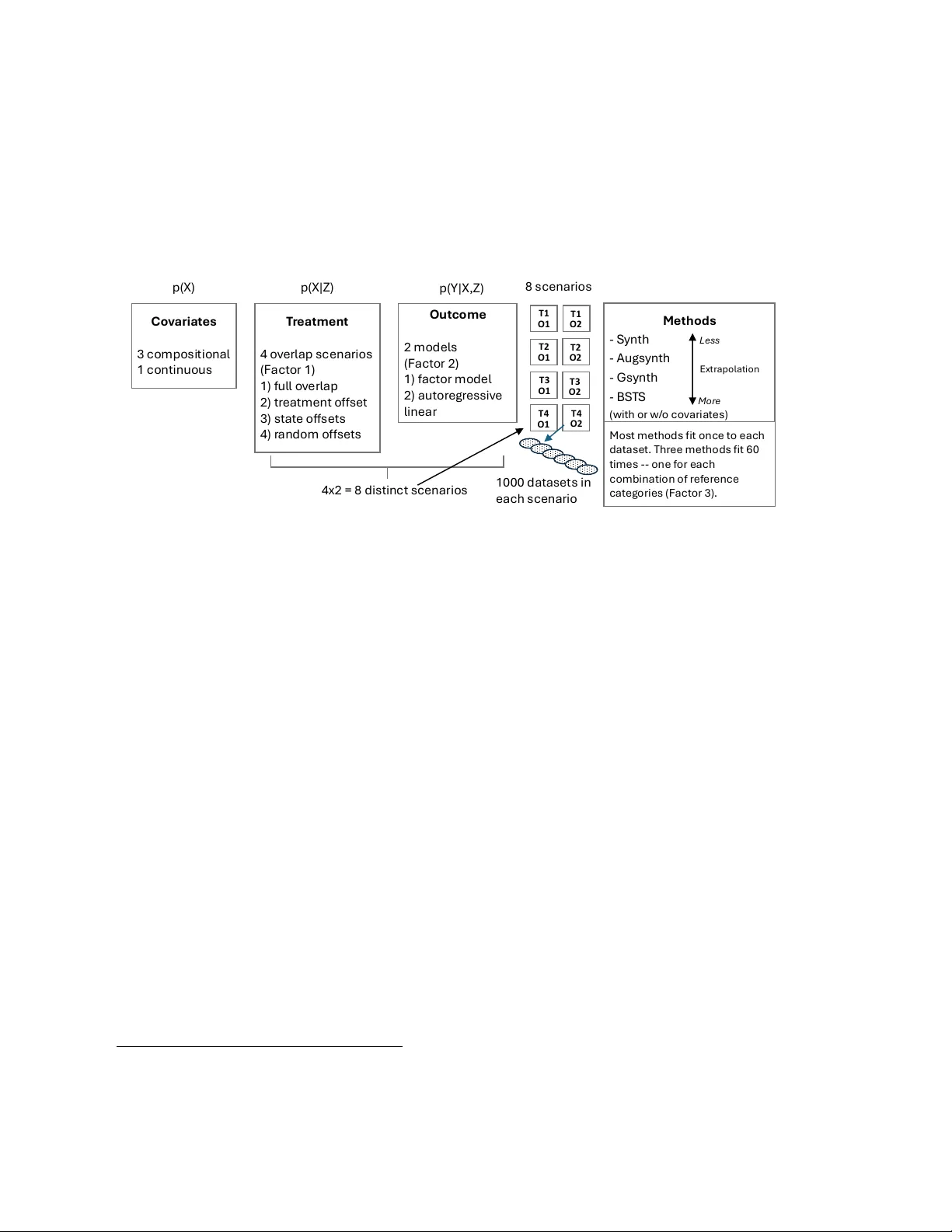
Syn thetic Con trol Misconceptions: Recommendations for Practice Rob ert Pic kett ∗ Jennifer Hill † Sarah Co wan ‡ Marc h 20, 2026 Abstract T o estimate the causal eﬀect of an in terven tion, researchers need to iden tify a con- trol group that represen ts what might ha ve happened to the treatment group in the absence of that in terven tion. This is c hallenging without a randomized exp eriment and further complicated when few units (possibly only one) are treated. Nev erthe- less, when data are a v ailable on units o ver time, syn thetic control (SC) methods pro vide an opp ortunit y to construct a v alid comparison b y diﬀeren tially w eighting con trol units that did not receive the treatment so that their resulting pre-treatmen t tra jectory is similar to that of the treated unit. The hop e is that this weigh ted “pseudo-coun terfactual” can serve as a v alid coun terfactual in the post-treatment time p eriod. Since its origin tw en t y years ago, SC has b een used ov er 5,000 times in the literature (W eb of Science, December 2025), leading to a proliferation of descrip- tions of the method and guidance on prop er usage that is not alw ays accurate and do es not alwa ys align with what the original developers app ear to ha ve intended. As suc h, a num b er of accepted pieces of wisdom ha ve arisen: (1) SC is robust to v arious implemen tations; (2) co v ariates are unnecessary , and (3) pre-treatmen t prediction er- ror should guide mo del selection. W e describ e each in detail and conduct simulations that suggest, both for standard and alternative implementations of SC, that these purp orted truths are not supported by empirical evidence and th us actually represen t misc onc eptions about b est practice. Instead of relying on these misconceptions, w e oﬀer practical advice for more cautious implemen tation and interpretation of results. Keyw ords: Syn thetic Control Metho ds, Sim ulation Study , Causal Inference, Longitudinal Data, Observ ational Study ∗ New Y ork Universit y , Cash T ransfer lab † New Y ork Universit y , Department of Applied Statistics, Social Science, and Humanities ‡ New Y ork Universit y , Department of Sociology and Cash T ransfer Lab 1 1 In tro duction In the tw en t y plus years since Abadie and Gardeazabal in tro duced synthetic con trol (SC) metho ds, researc hers hav e used the approach thousands of times. In 2021, SC w as cited b y Guido Im b ens as one of the most exciting prosp ects in econometrics in his Nob el Prize lecture ( Im b ens , 2021 ). The rapid rise in p opularit y of SC methods ha ve inspired a prolifer- ation of tec hniques and implementations that ha v e outpaced the literature ev aluating these approac hes in applied settings. The primary supp ort for these metho ds rests on proofs that p osit particular data-generating pro cesses, with surprisingly few ev aluations of how these metho ds p erform with ﬁnite pre-treatment observ ations and an unknown underlying data generating pro cess. 1 Brieﬂy , the goal of SC is to ﬁnd a “matc h” for a time series of a particular outcome v ariable prior to an in terv ention in a giv en treated unit. This ‘matc hed’ pre-treatmen t trend is then extrapolated forward in time to the p ost-treatment p erio d, which stands in for the h yp othetical time series in the absence of treatment (the counterfactual). Because it is virtually imp ossible to ﬁnd a single control unit that is a go o d match for the treated unit, w e instead generate a ‘synthetic’ matc h by taking a weigh ted a verage of un treated units on the basis of pre-treatment data. The causal eﬀect estimate is then constructed as the diﬀerence b et w een the outcomes for treated unit and the syn thetic con trol unit. In practice, researchers tend to estimate causal eﬀects that are the av erage of sev eral time- sp eciﬁc treatment eﬀects. Though the logic of SC is fairly straigh tforward, due to the generalit y of the theoretical guidance researchers face a num b er of practical decisions that may not hav e clearly deﬁned b est practices. This has caused some researchers to arriv e at a few misconceptions ab out b est practice in applied settings. • Misconception 1: SC is inv ariant to a n umber of implementation c hoices. This in- cludes the choi ce of algorithm to generate SC w eigh ts and the choice of reference category for categorical or comp ositional cov ariates. • Misconception 2: Including co v ariates is unnecessary , esp ecially if a close pre-treatment matc h for the outcome time-series can b e found without them. 2 • Misconception 3: The closeness of the pre-treatmen t match can b e used to adjudicate b et ween diﬀeren t SC metho ds as well as diﬀerent implemen tation choices within a giv en SC metho d. 1 F or notable exceptions, see Arkhangelsky et al. ( 2021 ); F erman ( 2021 ); F erman and Pin to ( 2021 ); F erman et al. ( 2020 ). 2 There are situations where including cov ariates is untenable, for instance when all pre-treatmen t out- come observ ations are included in the mo del ( Kaul et al. , 2022 ). Here we consider the standard implemen- tation of SC which summarizes the pre-treatment outcome series prior to estimation. F ollo wing F erman et al. ( 2020 ), researc hers may wish to consider these results against a sp eciﬁcation with all pre-treatmen t outcome observ ations and no co v ariates as a robustness c heck. 2 In this pap er, we conduct a simulation exercise to put these misconceptions to an empirical test. This pap er pro ceeds as follows: w e ﬁrst outline an empirical case that motiv ates our exploration. Then, after a brief exp osition of the inner w orkings of SC metho ds, we review these three misconceptions of SC implementation in more detail. W e then presen t evidence from an empirically calibrated sim ulation study that c hallenges these misconceptions in practice. Finally , we conclude with recommendations for practice. 1.1 Empirical Case: Alask a and the P ermanent F und Dividend T o motiv ate our exploration, w e draw on the empirical case of Alask a’s P ermanen t F und Dividend (PFD). In 1976, Alask a b egan inv esting a p ortion of its mineral reven ues into a div ersiﬁed fund in order to ensure long-term ﬁnancial stabilit y for the state. Since 1982 Alask a has paid out a p ortion of the fund’s earned interest to eligible Alask an residents as a dividend, with paymen ts ranging from ab out $ 1040 in 1984 to ab out $ 3,800 in 2022 (in 2026 inﬂation adjusted dollars). 3 This pa ymen t pro vides a p er-family inﬂux of cash roughly comparable to or exceeding pa yments from ma jor so cial support programs including the earned income tax credit (EITC) and in kind pa yments from the supplemen tal nutrition assistance program (SNAP) ( Co w an and Douds , 2022 ). A num b er of pap ers ha ve attempted to identify the causal eﬀects of these annual cash transfers by comparing Alask a b efore and after 1982 on a num b er of outcomes. In particular, researchers hav e used SC methods to explore the PFD’s eﬀect on crime ( Dorsett , 2021 ) and lab or mark et participation ( Jones and Marinescu , 2022 ). T o ensure our sim ulations are in line with practical applications, w e use empirical data from Alask a to calibrate our sim ulation exercise (see Section 4 for details). 4 2 Syn th and its Implemen tation There are a n um b er of statistical pack ages that estimate treatment eﬀects using synthetic con trol metho ds, eac h with slight v ariations. Giv en the ov erwhelming p opularity of the original work by Alb erto Abadie and coauthors 5 ( Abadie and Gardeazabal , 2003 ; Abadie 3 P a ymen ts in several other recent years, for example 2020 and 2025, were also on the order of $ 1000. 4 W e fo cus on this Alask a case study b ecause it has b een used in previous SC work and giv es us a chance to ground our simulations in existing data. W e are not, how ever, claiming that the issues raised in this pap er are the only ones that might be raised with regard to the Alask a PFD. F or instance, the creation of the fund is one of numerous ma jor policy changes in Alask a in the wak e of the oil b o om, including ma jor revisions to the tax co de in 1975 and a complete rep eal of the state income tax in 1980. This raises additional concerns ab out the volatilit y of the pre-treatmen t outcome series and anticipation eﬀects due to multiple related p olicies b eing enacted o ver a short perio d of time just b efore the PFD was rolled out. Those issues hav e b een discussed more thoroughly in the SC literature ( Abadie , 2021 ). The purp ose of this pap er is to focus on the more insidious problems common across a broad range of potential SC applications. 5 The ﬁrst reference to this approach as well as the Synth pack ages developed in Stata and R to implemen t it ( Abadie and Gardeazabal , 2003 ) has b een cited more than 7000 times and the seminal 2010 pap er ( Abadie et al. , 2010 ) has b een cited more than 8000 times. The Synth softw are has b een downloaded more than one million times in Stata and o v er 180,000 times in R. 3 et al. , 2010 ) we use those pack ages as our starting p oin t for describing the metho d. Assume we can write a factor mo del for an outcome Y i,t for unit i in y ear t as Y i,t = δ t + θ t Z i + λ t µ i + α i,t D i,t + ϵ i,t , where δ t is an unobserved factor shared across units (year ﬁxed eﬀect), Z i is a vector of r observ ed co v ariates (observed once p er unit pre-treatment), θ t is an unknown v ector of r time trends shared across units, µ i is a v ector of f unobserv ed co v ariates (observed once per unit), and λ t is an unknown vector of f time trends shared across units. W e will sort the units so the treated unit is the ﬁrst ( i = 1), follo wed b y all control units ( i ∈ { 2 , 3 , . . . n } ). D i,t is a treatment indicator with v alues of 1 when i = 1 (the treated unit) and t > T 0 where T 0 is the last pre-treatmen t p eriod (with 1 ≤ T 0 < T ), making α i,t is the causal eﬀect (deﬁned below). Finally , ϵ i,t is a vector of unobserv ed transitory shocks with mean zero. W e will use Y 1 ,t (1) and Y 1 ,t (0) to denote the potential outcome within the treated state for the treated and con trol conditions, resp ectively , at time t , with α i,t = Y 1 ,t (1) − Y 1 ,t (0). This set-up assumes that there are no treatment eﬀects before the treatmen t starts, that the treated unit is contin ually treated after the treatment starts, and that the treatment has no eﬀect on con trol units. The goal of syn thetic control is to construct a syn thetic coun terfactual unit out of a w eighted combination of control units, restricting these control unit weigh ts to b e conv ex (they are p ositiv e and sum to one) to a void extrap olation. Sp eciﬁcally , if we ﬁnd a vector of non-negative weigh ts, w ∗ j , for each con trol unit j , sub ject to Σ w ∗ j = 1 suc h that J +1 X j =2 w ∗ j Y j,t ≈ Y 1 ,t for all t ≤ T 0 , and J +1 X j =2 w ∗ j Z j ≈ Z 1 then Y 1 ,t (0) − P J +1 j =2 w ∗ j Y j,t will b e b ounded, small, and asymptotically approac h zero as the n umber of pre-interv ention p erio ds gets large relative to the scale of the transitory sho cks, ϵ i,t ( Botosaru and F erman , 2019 ). If these conditions hold, w e can estimate the causal eﬀect as, ˆ α i,t = Y 1 ,t − J +1 X j =2 w ∗ j Y j,t for t ∈ { T 0 + 1 , . . . , T } . 6 Abadie et al. ( 2010 ) suggest that these w eigh ting conditions ma y not hold exactly in practice, and it is up to researchers to ev aluate “if the c harac- teristics of the treated unit are suﬃciently matched by the syn thetic control,” without sp eciﬁc guidelines for ho w to mak e that determination. W e will refer to the amount of 6 Abadie et al. ( 2010 ) also pro v e that the estimator works for an autoregressive mo del with time-v arying 4 pre-treatmen t mismatch b etw een the synthetic con trol and treated units as the amoun t of ‘outcome imbalance,’ and we will measure this imbalance with the pre-treatmen t ro ot mean squared prediction error (RMSPE) 7 giv en by v u u t 1 T 0 T 0 X t =1 ( Y 1 ,t − J +1 X j =2 w ∗ j Y j,t ) 2 In order to ﬁnd the SC w eigh ts, we let ¯ Y K M j represen t M linear combinations of pre- treatmen t outcomes Y i,t (usually just the state-sp eciﬁc mean prior to treatment, 1 T 0 P T 0 t =1 Y i,t ), and then let X 1 = ( Z 1 , ¯ Y K M 1 ) for the treated unit, and X 0 b e the same for eac h of the J control units, i.e., X 0 = ( Z i  =1 , ¯ Y K M i  =1 ). W e then wan t to c ho ose weigh ts W to mini- mize some distance b et ween X 1 and X 0 W . Because we cannot guarantee a match across all co v ariates, we wan t to use a vector of v ariable imp ortance weigh ts V to prioritize our matc hing. W e can then deﬁne a v ariable loss function that reﬂects these priorities: ∥ X 1 − X 0 W ∥ v = p ( X 1 − X 0 W ) ′ V ( X 1 − X 0 W ) T o ﬁnd w eights W ∗ and V ∗ w e can use a tw o-step optimization pro cess. 8 The outer lev el will b e a non-linear optimization that ﬁnds V ∗ = arg min v 1 T 0 T 0 X t =1 ( Y 1 ,t − J +1 X j =2 W ∗ ( V ) Y j,t ) 2 . The inner level of the optimization will b e a quadratic optimizer that ﬁnds W ∗ ( V ) = arg min w ∥ X 1 − X 0 W ∥ v . The nested optimizer is initialized with empirically deriv ed V weigh ts, whic h we will refer to as ‘regression weigh ts.’ This initial V vector is set by taking standardized summed squared regression co eﬃcien ts for all cov ariates in X predicting pre-treatment outcomes in co v ariates and co eﬃcien ts, Y i,t (0) = Y i,t − α i,t D i,t Y i,t +1 (0) = λ t Y i,t (0) + β t +1 Z i,t +1 + µ i,t +1 Z i,t +1 = γ t Y i,t (0) + Π t Z i,t + v i,t +1 . Both sp eciﬁcations assume shared trends in cov ariates Z . W e fo cus for now on the factor mo del for now as it more closely resembles their implementation but the autoregressiv e role will pla y a role in our sim ulation. 7 Other measures of imbalance are p ossible, and indeed diﬀeren t SC pack ages deﬁne diﬀerent balance metrics. W e use RMSPE here because it is common in the literature and in implementations of SC metho ds. 8 There is some con tro v ersy here. Some scholars hav e suggested that this step should b e approached explicitly as a bilev el optimization problem since the standard approac h rarely ﬁnds optimal solutions (these optimal solutions are often corner cases where all weigh t is assigned to one predictor) ( Malo et al. , 2024 ). Others hav e suggested disregarding V entirely , simply setting each v alue of the v ariable imp ortance v ector to 1 ( Ben-Mic hael et al. , 2021 ). 5 all y ears. 9 Sp eciﬁcally , let X b e X 1 app ended to X 0 , ( X 0 , X 1 ), and let X ∗ b e X where all columns ha v e b een divided b y their standard deviations, plus an in tercept column. Then, β k,t = ( X ′ ∗ X ∗ ) − 1 ( X ′ ∗ Y j,t ) for all cov ariates k in X and all t ∈ { 1 , . . . , T 0 } . Finally , let the initial v alue for V b e P t β 2 k,t P k P t β 2 k,t (see also Bohn et al. ( 2014 ); Kaul et al. ( 2022 )). While this empirically initialized nested optimization pro cess is the default implemen- tation used in R, it is not the default for Stata. 10 In Stata, the V matrix is simply set to the empirical estimate P t β 2 k,t P k P t β 2 k,t and a single non-linear optimizer is used to ﬁnd W ∗ conditional on the regression v ariable weigh ts V . 3 Misconceptions of Syn thetic Con trol Ha ving review ed the general set-up for SC metho ds, w e now turn to a discussion of the three misconceptions we see guiding implementation of SC metho ds in practice. 3.1 Misconception 1: Syn thetic Con trol is Robust to Implemen- tation Choices Syn thetic con trol is no w a common to ol among applied researchers, who face many imple- men tation decisions with unclear applied guidance. In this section, w e discuss t wo suc h c hoices: whic h optimization pro cess to use for v ariable w eights, and which reference cate- gory to omit when including categorical or comp ositional cov ariates (or indeed whether to omit a reference category at all). 3.1.1 Misconception 1a: Nested vs Regression W eigh ts are In terc hangeable Abadie et al. ( 2010 , p p. 496) note that the pro ofs of Syn thetic Control’s asymptotic p erformance are v alid for an y c hoice of the v ariable w eigh ts v ector V . This can lead applied researc hers to incorrectly assume that Synth is relatively in v ariable to choices for sp eciﬁc V v ectors - thus treating the nested optimizer, ‘regression weigh ts,’ and a uniform V matrix as somewhat exc hangeable. Diﬀerences in how SC is implemented across the t wo most p opular statistical pack ages (‘Syn th’ in R and Stata) - without clear instructions for when to use one implemen tation or pack age ov er another - makes matters worse. R defaults to the nested optimizer and can only implemen t ‘regression w eights’ by manually inputting them as user-deﬁned custom weigh ts. Stata defaults to ‘regression w eigh ts’ but can use nested weigh ts by sp ecifying the ‘nested’ option. 11 9 If the regression is inestimable, the nested optimizer is instead initialized with uniform V weigh ts. 10 Y ou can implement this tw o-step optimization in Stata by using the ‘nested’ argument. 11 The Stata do cumentation ( https://web.stanford.edu/ ~ jhain/fqa.htm ) provides little guidance as to when y ou should use ‘nested’ vs ‘regression’ weigh ts, simply suggesting ‘nested’ weigh ts as a strategy to impro v e pre-treatmen t ﬁt. 6 In their original pap er, how ev er, Abadie et al. ( 2010 , pp. 496) also p oint out that the c hoice of V weigh ts inﬂuences the mean squared error of the estimator, though w e hav e not seen an empirical assessmen t of ho w substan tial this inﬂuence migh t b e. Th us, for our ﬁrst test, we explore the degree to which SC’s performance depends on choices of V in order to ev aluate whether or not suc h decisions are reasonably inconsequen tial. 3.1.2 Misconception 1b: Reference Category Choice is Inconsequen tial Next, w e turn to the assumption regarding the c hoice of whic h reference category to exclude when including comp ositional or categorical cov ariates in SC. Categorical v ariables (e.g., race, gender, income brac ket, marital status, etc.) often serve as imp ortant predictors of the outcome. F or an example, Jones and Marinescu ( 2022 ) when estimating the eﬀect of the Alask a Permanen t Dividend on labor market participation, include three compositional v ariables: the percentage in age groups (with four categories), education groups (with three categories), and industry groups (with ﬁve categories). When categorical or comp ositional v ariables are included in a linear regression, re- searc hers t ypically omit one category as a reference category . No matter what category is omitted, the predictions from such a mo del w ould not b e aﬀected and the interpretations of all b etw een group comparisons w ould b e recov erable. In contrast, the results of a standard synthetic control analysis ar e sensitive to whic h reference category a researc her chooses. While a regression will enco de the same infor- mation regardless of the reference category omitted, the sums of squared co eﬃcien t mag- nitudes, and thus regression v ariable w eights, are not identical across these settings. F or a sp eciﬁc example, consider one outcome v ariable Y , and mutually exclusiv e and com- pletely exhaustiv e dic hotomous regressors X 1 , X 2 , and X 3 suc h that X 1 + X 2 + X 3 = 1. If E [ Y | ( X 1 = 1)] = 10; E [ Y | ( X 2 = 1)] = 1; E [ Y | ( X 3 = 1)] = − 5 then w e can write equiv alen t regressions: Y = − 5 + 15 ∗ X 1 + 6 ∗ X 2 + ϵ Y = 1 + 9 ∗ X 1 − 6 ∗ X 3 + ϵ Y = 10 − 9 ∗ X 2 − 15 ∗ X 3 + ϵ Though these regressions provide equiv alent conditional exp ectations of Y , the sum of squared coeﬃcients clearly v aries: 261 in the ﬁrst, 117 in the second, and 306 in the third. W e could consider a similar example that includes another predictor α but k eeps the co eﬃcients for X ’s the same: Y = − 5 + 10 ∗ α + 15 ∗ X 1 + 6 ∗ X 2 + ϵ Y = 1 + 10 ∗ α + 9 ∗ X 1 − 6 ∗ X 3 + ϵ Y = 10 + 10 ∗ α − 9 ∗ X 2 − 15 ∗ X 3 + ϵ Though these regressions provide the same information (i.e., reco ver the same contrasts and produce the same predicted v alues), the c hoice of omitted category can change the implied imp ortance of α relative to X in the most p opular version of the syn thetic controls 7 implemen tation. In the ﬁrst equation, α mak es up 10 2 10 2 +6 2 +15 2 ≈ 28% of the total v ariable w eight, in the second it mak es up 10 2 10 2 +9 2 +6 2 ≈ 46% of the w eigh t, and in the third it makes up 10 2 10 2 +15 2 +9 2 ≈ 25% of the w eigh t (see Figure 1 ). In general, if w e c ho ose to omit a category where the conditional exp ectation of Y for that category is farther a w a y from the mean of conditional exp ectations of Y for eac h possible omitted category w e will increase the relativ e contribution of the categorical v ariable X to the v ariable weigh ts V . 1 2 3 0.00 0.25 0.50 0.75 1.00 P ercentage Model V ariable X a Figure 1: Con tributions to V Imp erfect matching b etw een treated and synthetic units pro duces a second la yer of uncertain ty that is indep enden t of the V matrix. The standard logic is that if y ou matc h on all but one category of a comp ositional or categorical v ariable, the linear dep endence among categories will ensure that y ou also match on the category left out. Unfortunately , the curse of dimensionality makes ﬁnding a p erfectly matc hing conv ex com bination of con trol units imp ossible in many applied settings. In practice, man y imp erfect solutions are p ossible, and the sp eciﬁc solution will dep end on which categories are included in the analysis. Th us, selecting diﬀerent reference cat- egories will pro duce slightly diﬀerent syn thetic con trol w eights that in turn yield slightly diﬀeren t matches b et w een the treated and synthetic con trol unit. These diﬀeren t matches pro duce diﬀerent causal estimates. 3.2 Misconception 2: Co v ariates are not necessary when using SC In their pro of for when the synthetic con trol approach can b e unbiased, Abadie et al. ( 2010 ) sho w that if the SC assumptions hold the bias in tro duced by omitting co v ariates go es to zero as the n um b er of pre-treatment time p erio ds grows large relative to transient sho c ks in the outcome (see also Botosaru and F erman ( 2019 ); F erman and Pin to ( 2021 ); Kaul et al. ( 2022 )). The intuition b ehind this result is that b ecause the outcome series is of primary interest, cov ariates only matter to the exten t that they inﬂuence the outcome 8 time series, and if the Syn thetic Con trol metho d can p erfectly repro duce the un treated outcome time series, additionally matching on co v ariates is sup erﬂuous. In other w ords, if y ou can closely align the treated and synthetic outcome tra jectories for a long enough time b efore treatmen t — and the data generating pro cess follows either a factor mo del or a sp eciﬁc autoregressive mo del ( Abadie et al. , 2010 ) — you m ust also hav e aligned on the factors that are relev an t for pro ducing that outcome. This has led to some to de-emphasize the imp ortance of co v ariates in SC analyses ( Botosaru and F erman , 2019 ; Gilc hrist et al. , 2023 ). Others ha ve recommended excluding co v ariates in some circumstances for practical reasons, e.g., when opting to balance on all pre-treatmen t outcomes, which ma y also reduce v ariation in results across plausible implementations ( F erman et al. , 2020 ). W e oﬀer tw o words of caution for those considering omitting co v ariates. First, co v ari- ates may ha ve substantial eﬀects on the p erformance of the estimator, esp ecially when the pre-treatment time series is short ( Kaul et al. , 2022 ). Second, the pre-treatmen t ﬁt diagnostic may b e an unreliable measure of how closely the synthetic con trol resembles the coun terfactual when the pre-treatmen t time series is short ( Abadie , 2021 ). Consider an extreme example where we ha ve observ ations for a single time p oin t prior to treatment and the treated unit’s data absen t treatment can b e written as: Y 1 ,t (0) = 1 + ϵ 1 ,t ; ϵ 1 ,t ∼ N (0 , 1) and data for all con trol units can b e written as: Y j,t = 0 + ϵ j,t ; ϵ j,t ∼ N (0 , 1) In this scenario, if w e hav e a suﬃcient n umber of control units it is quite likely that w e can ﬁnd a p erfect match for the treated unit’s single pre-treatment observ ation. That said, we’v e constructed this p erfect match by selecting con trol units with randomly large v alues of ϵ j, 1 to match the structurally large v alues of Y 1 , 1 . W e’v e eﬀectively o verﬁt our mo del to transien t sho cks rather than structural v ariation in the outcome series. When w e extrap olate the p ost-treatmen t syn thetic control time series, the exp ected v alue of P J +1 j =2 w ∗ j Y j,t will return to zero, while the exp ected v alue of the true counterfactual Y 1 ,t (0) will remain 1. Thus, whatever causal estimate w e generate will b e upw ardly biased by 1 unit in exp ectation. In sum, we can hav e an exact empirical match while ha ving a remark ably p o or match in exp ectation. When there are few pre-treatmen t p erio ds, including relev an t co v ariates may reduce o verﬁtting b y providing additional information. W e explore whether the logic of this to y example holds in general practice in our sim ulation results. 3.3 Misconception 3: Lo w er Pre-T reatmen t Outcome Im balance Suggests Low er Absolute Bias In their original pap ers describing the metho d Abadie et al. ( 2015 , 2010 ) note that if pre-treatmen t outcome im balance is p o or, syn thetic con trol methods are unlik ely to pro- duce unbiased estimates of the treatmen t eﬀect. Ov er time, though, this general caution 9 seems to hav e been in terpreted as a recommendation to use pre-treatment outcome im- balance as a metric for mo del selection. F or example, Panagiotoglou and Lim ( 2022 ) and Oliphan t ( 2022 ) restrict the years they use for pre-treatmen t opimization to impro v e their pre-treatmen t outcome imbalance. Ov eremphasizing the go o dness of ﬁt metric in this w ay is likely to lead to ov erconﬁdence in the mo del results and p otential o verﬁtting to idiosyn- cratic changes in the outcome v ariable ov er short durations. An alternative in terpretation of this strategy of omitting pre-treatmen t data to impro ve goo dness of ﬁt is to view the exercise as a failed pre-treatment placebo test, as it suggests that the syn thetic control mo del is not pro viding reliable pre-treatment predictions across all av ailable data. Others may place too m uch emphasis on pre-treatment outcome im balance in subtler w ays. F or example, Gilc hrist et al. ( 2023 ) and Donohue et al. ( 2019 ) tie the plausibil- it y of synthetic con trol estimates to lo w pre-treatmen t im balance. Although results from syn thetic control mo dels that pro duce large deviations from the pre-treatment time series should b e view ed sk eptically , closely repro ducing a short pre-treatmen t time series is not suﬃcien t for trustw orth y results. Indeed, o ver short durations these mo dels can perfectly ﬁt idiosyncratic noise, producing inaccurate estimates of the future time series. Zimmerman et al. ( 2021 ) and T ownsend et al. ( 2022 ) go further, relying on pre-treatment mean squared prediction error to determine whether or not they include co v ariates in their analyses. Bal- ancing on co v ariates pro vides the opportunity for additional veriﬁcation in the case that mo dels ﬁt to short pre-treatmen t outcomes are in fact pro viding reasonable estimates of the structural v ariation for the treated unit. Simply discarding them when the co v ariates suggest worse ﬁts ignores this p otential w arning. Others rely on pre-treatment balance to guide mo del ﬁtting decisions. Opatrny ( 2021 ) determines which control units to include by examining whic h set pro duces the low est pre- treatmen t RMSPE, and Islam ( 2019 ) and Propheter ( 2020 ) rely on pre-treatmen t RMSPE for v ariable selection — including the set that produces the lo west pre-treatment prediction error. Ideally , these decisions would instead b e made according to theories ab out the pre- treatmen t data generating process, or by follo wing a set pro cedure to minimize p otential bias from sp eciﬁcation searc hing ( F erman et al. , 2020 ). Relatedly , Parast et al. ( 2020 ) dev elop metrics for iden tifying when pre-treatmen t bal- ance is suﬃcient for accepting the syn thetic con trol estimate - but also note that mini- mizing im balance ma y not alw a ys pro duce the most plausible estimate (e.g., using few er pre-treatmen t perio ds). While the intuition b ehind using pre-treatment RMSPE in these w ays is clear, w e hav e not seen this relationship explicitly tested in the literature. In the results b elow, we explore whether pre-treatment outcome im balance is predictive of p ost- treatmen t model p erformance, or whether researchers should only rely on pre-treatment outcome imbalance to iden tify when synthetic con trol metho ds are failing entirely . 4 Sim ulation T o b etter understand the p otential eﬀects of these misconceptions w e conducted a simu- lation analysis to compare the p erformance of a v ariety of approac hes relativ e to a kno wn 10 truth. W e ground our analysis in a facsimile of an observed empirical scenario to better understand how these misconceptions may play a role in practice. The empirical setting w e use to calibrate our sim ulation fo cuses on the eﬀect of the 1982 Alask an P ermanent F und Dividend. In particular, w e use data from the Current P opulation Surv ey (CPS) to estimate pre-treatment relationships b et ween co v ariates and state-sp eciﬁc trends and base our sim ulated data on these estimates. W e outline this pro cess in the next sections and provide further details in App endix A . 4.1 Sim ulation Ov erview Our simulation is designed to explore the tenabilit y of the three misconceptions describ ed ab o ve. As such it is designed with three factors, eac h of which controls either aspects of the data generating process or implemen tation c hoices that could impact p erformance of the treatment eﬀect estimators. Since the original implementation of SC app ears to rest hea vily on the no-extrap olation assumption, our ﬁrst simulation factor creates a range of scenarios that either fully support or violate that assumption. As such this factor creates v ariation in the researcher’s ability to create a synthetic con trol that appro ximates the treated unit prior to treatmen t exp osure. W e ac hieve this b y v arying the empirical o v erlap b etw een the treated and control states when generating the cov ariate distributions. The second simulation factor is implemented in tw o diﬀeren t mo dels for the data gen- erating pro cesss (DGP) for the outcome. The ﬁrst is a factor mo del that closely aligns to the pro ofs laid out by ( Abadie et al. , 2010 ). The second is a linear mo del that resem bles standard regression analyses, but for whic h there is no clear asymptotic pro of as it relates to SC. The third sim ulation factor explores model performance across omitted reference categories for comp ositional or categorical v ariables. W e ev aluate the p erformance of four metho ds (each of whic h is implemen ted in several w ays) across these three sim ulation factors. These four metho ds v ary in the degree to whic h they allow for extrapolation from control units in order to ﬁt the treated outcome series. In order from least extrap olation to most extrap olation, w e test Syn th, Augsynth, GSynth, and Ba yesian Structural Time Series (BSTS). In addition, w e test the p erformance of eac h of these metho ds with and without cov ariates. An o v erview for this sim ulation setup can b e found in Figure 2 . W e describ e each of these steps in the follo wing sections and additional detail can b e found in Appendix A . In App endix B we additionally in v estigate mo del p erformance for our sim ulation settings across three diﬀerent pre-treatmen t time series durations. 4.2 Sim ulation Calibration W e calibrate our sim ulations to “real life” b y ﬁtting mo dels to 10 years of data from the Curren t P opulation Survey Ann ual So cial and Economic Supplemen t (CPS-ASEC). W e then use estimates of those mo del parameters to sim ulate 100 years of new data. Because w e are primarily interested in the Permanen t F und Dividend (PFD), w e use the 10 y ears of 11 Figure 2: Sim ulation Ov erview C o v a r i a t es 3 c o m po s i t io n a l 1 c o n t in uo us T r e a t m e n t 4 o v e r l a p s c e n a r io s ( F a c to r 1 ) 1 ) f ul l o v e r l a p 2 ) tr e a tm e n t o f f s e t 3 ) s ta te o f f s e ts 4 ) r a n do m o f f s e ts p( X ) p( X | Z ) O u t c o m e 2 m o d e l s ( F a c t o r 2 ) 1 ) f a c t o r m o de l 2 ) a ut o r e g r e s s iv e l in e a r 4 x2 = 8 dis t in c t s c e n a r io s p( Y | X , Z ) M e t h o d s - S y n t h - A ug s y n t h - G s y n t h - B S T S ( w i t h o r w / o c o va r i a t e s ) 8 s c e n a r io s L e s s Mo r e E x t r a p o lat i o n T1 O1 T4 O2 T2 O2 T3 O2 T4 O1 T2 O1 T1 O2 T3 O1 M o s t m e t h o d s f i t o n c e t o e a c h d a t a s e t . T h r e e m e t h o d s f i t 6 0 t i m e s -- o n e f o r e a c h c o m b i n a t i o n o f r e f e r e n c e c a t e g o r i e s ( F a c t o r 3 ) . 1 0 0 0 d a t a s e t s in e a c h s c e n a r io data surrounding the implemen tation of the PFD, 1977–1986. 12 Our outcome v ariable of in terest is the prop ortion in the state who are employ ed part-time. The av erage prop ortion w orking part-time across all states in the CPS b et ween 1977 and 1986 is 9.5% with a stan- dard deviation of 1.7%. F or Alask a sp eciﬁcally , the mean is 8.4% with a standard deviation of 0.9%. In our mo dels w e include co v ariates for the following: the racial comp osition of states (percent White, Blac k, and Other, whic h sum to 100%); the educational comp osi- tion of states (percent with less than high sc ho ol education, high sc ho ol, some college, and college or more); the comp osition of p eople w orking in ﬁve industry categories (the per- cen t w orking in agriculture, forestry , ﬁsheries, mining, construction, and manufacturing; the percent working in transp ortation, communications, other public utilities, wholesale trade, or retail trade; the p ercen t working in ﬁnance, insurance, real estate, business and repair services, and p ersonal services; the percent working in entertainmen t and recreation services, professional and related services, public administration, active dut y military , and exp erienced unemplo yed not classiﬁed by industry; and the percent not curren tly in the lab or force; and the av erage self-reported annual wage by state. The inclusion of these three comp ositional cov ariates generates 60 p ossible combinations of reference categories. 13 Our observed time series only spans 10 years (5 years pre-treatment and 5 years p ost- treatmen t), but we need suﬃcient data to estimate synthetic control metho ds. Therefore, 12 1977 w as the ﬁrst y ear Alask a w as included in the CPS-ASEC. 13 Three race categories b y four education categories by ﬁve industry categories pro duces 60 p ossible reference category com binations. 12 w e ”artiﬁcially extend” our sim ulated data. T o do this, w e pretend that our 10 y ears of data actually spanned 100 years (50 pre-treatmen t and 50 p ost-treatmen t). 14 Therefore we relab el observed y ear 1977 as our 0 th y ear in our sim ulation w orld (50 years pre-treatmen t) and 1986 as our 100 th y ear in our sim ulation w orld (50 y ears p ost-treatmen t). Each one y ear gap in the real world then corresp onds to a 10 year gap in the sim ulated world. This means that our sim ulation mo del relies on interp olations betw een observ ed y ears rather than extr ap olations b ey ond the range of our observed co v ariate data. This helps to ensure that the cov ariate data used reﬂect conditions that are likely to exist in the world. 4.2.1 Sim ulating Co v ariates and Inducing T reatmen t Assignmen t T o build the co v ariate p ortion of our data generating pro cess while calibrating to the Alask a data, w e start b y considering a factorization of the join t lik eliho o d of the co v ariates in to the follo wing distributions: the conditional distribution of industry giv en state and y ear; the conditional distribution of education giv en industry , state, and year; the conditional distri- bution of race given industry , education, state, and y ear; and the conditional distribution of wage given the rest. The ﬁrst three conditional distributions are mo deled as Dirichlet regressions and the last as a standard linear regression with normal errors. Sampling pre- dicted v alues from these mo dels and their asso ciated uncertaint y parameters will allow us to preserve observed relationships b etw een cov ariates in our simulated data. The strength of synthetic con trol metho ds lies in their abilit y to reconstruct synthetic coun terfactual units that are plausibly similar to the treated unit prior to treatment. It is crucial, then, to ev aluate how w ell these mo dels can reco ver these plausible counterfactuals when treated units are v ery similar to donor control units, v ersus when treated units are less similar. Recall that SC do esn’t require any one comparison unit to b e v ery similar to the treated unit but rather that a weigh ted com bination of the comparison units is similar to the treated unit. If the comparisons states are systematically diﬀerent, then this w eigh ted a verage will require extrap olation b eyond the observ ed co v ariate space for the con trols in order to create a pseudo-con trol that is suﬃcien tly similar to the treated unit. T o ev aluate the p erformance of these mo dels under diﬀerent conditions, w e generate data from a range of scenarios that v ary based on the exten t to which our treated state (Alask a) is more or less similar in its co v ariate v alues to the 49 other p otential donor con trol states. W e op erationalize these diﬀerences by ﬁtting models with v arying ﬁxed eﬀects structures to the observed data, whic h then inform the mo dels from which w e generate sim ulated data. W e construct four suc h scenarios: 1. In the ful l overlap scenario we omit all state ﬁxed eﬀects from our mo dels th us the structural v ariation in pre-treatment co v ariates for treated and control units is forced to b e identical. 14 While studies with one hundred y ears of data may not o ccur often, recall that synthetic controls can b e used in a wide v ariet y of circumstances with time trends. F or instance, the data could b e measured in minutes, hours, days, or w eeks. In those circumstances, 100 pre-treatment ”time p erio ds” could easily o ccur. 13 2. In the tr e atment oﬀset scenario the pre-treatment co v ariate mo dels allow for a distinct in tercept only for the treated unit (i.e. it alone has a state ﬁxed eﬀect). 3. In the state oﬀset scenario the pre-treatmen t cov ariate mo dels include a state ﬁxed eﬀect for eac h state. This is the closest scenario to the empirically observ ed ov erlap. 4. In the r andom oﬀset scenario the models include a state in tercept randomly dra wn from a shared distribution. By randomly assigning state in tercepts w e allow for idiosyncratic diﬀerences b et ween states within an y giv en simulation dataset, but set the exp ectation of those diﬀerences to b e zero across the full set of simulations. T o sim ulate cov ariate data, we ﬁrst ﬁt eac h mo del based on the empirical data and mo del sp eciﬁcations describ ed ab o v e. W e then use the parameter estimates as means when dra wing co eﬃcien ts for eac h regression model (dra wn from a multiv ariate normal distribution) that simulates 100 years of data. W e can then draw from a Dirichlet (or normal) distribution conditional on these parameters and the observed data. W e pro vide further details in App endix A. 4.2.2 Sim ulating outcomes and treatmen t eﬀects After generating sim ulated co v ariates, our next step is to simulate outcomes, conditional on the co v ariates. As our second sim ulation factor, w e sim ulate outcomes in eac h of tw o diﬀeren t wa ys to reﬂect slightly diﬀeren t assumptions about the nature of the data generat- ing pro cess. One approach assumes an autoregressiv e linear model and the second assumes a factor mo del (consisten t with the original SC assumptions). As with the cov ariate gen- eration, we start b y ﬁtting the assumed mo del to Alask a. T o a void incorp orating an y eﬀects of the true PFD p olicy on the outcome, we only use CPS-ASEC (Alask a) data from years 1977 through 1981 to ﬁt these outcome mo dels. F or the outcome mo dels we do not incorp orate any systematic v ariation across states. Th us, in our four co v ariate scenarios, the outcome mo del is the same for all states; therefore, the diﬀerences b et ween states with regard to outcome v ariables will only o ccur in situations where their co v ariates hav e b een mo deled to b e systematically diﬀeren t. In this sense, these simulations pro vide a generous testing ground for synthetic con trols b ecause if there is ov erlap with resp ect to co v ariates there should also b e ov erlap with resp ect to outcomes. F or the autoregressiv e model, we regress the prop ortion w orking part-time on com- p ositional industry , education, and race v ariables as w ell as our con tinuous a verage wage v ariable. 15 F or the factor mo del, w e ﬁrst calculate state-sp eciﬁc pre-treatmen t means for eac h of our co v ariates in the CPS data. W e then regress the prop ortion w orking part time on year, these state-speciﬁc pre-treatmen t means, and the interaction betw een y ear and these pre-treatment means. As with the co v ariates, w e generate sim ulated outcome v ariables b y dra wing co eﬃcients from their estimated m ultiv ariate normal distribution and 15 Though the proportion w orking part-time is constrained to b e within the range [0,1], w e ﬁt linear regressions for simplicit y . 14 then drawing from a normal distribution conditional on those parameter v alues and the data. Finally , for eac h outcome sim ulation mo del, we add a constan t treatmen t eﬀect for sim ulation years ≥ 50 in the state of Alask a equal to t wo times the observ ed standard deviation of the prop ortion working part-time in Alask a in the CPS-ASEC for years 1977 through 1986. 16 Our simulations will examine how accurately eac h method can replicate this ground truth. In all, the tw o types of outcomes (factor tw o) generated for each of four co v ariate scenarios (factor one) pro duce eigh t distinct simulation scenarios. T o make comparisons as clear as p ossible, cov ariate v alues are iden tical for each pair of outcomes within the four co v ariate scenarios. W e conduct this sim ulation 1,000 times, pro ducing 8 outcome (factor vs autoregressiv e) b y co v ariate (“full o verlap”, “treatmen t oﬀset”, “state oﬀset”, and “random oﬀset”) scenarios eac h with 1,000 sim ulated datasets. Within each of the 8 sim ulation scenarios that capture v ariation in sim ulation factors 1 and 2, we p erform a test of the implications of the v ariation induced b y factor 3, which fo cuses on reference category c hoice. In particular, for eac h of these datasets, we generated a verage causal estimates for all 60 possible reference category com binations for methods that v ary in the w ays that they handle such co v ariates (describ ed in the next section). The resulting uncertain ty across these 60 mo dels then gives us an assessment of ho w sensitiv e these synthetic control causal estimates are to reference category choice. 4.3 Metho d Details Ov erall w e tested t w elv e approac hes. Nine of these implemen tations generate consisten t estimates regardless of omitted reference categories; three do not (describ ed b elo w) and th us w ere used in our examination of the implications of reference category choice (factor 3). W e select this set of implementations b ecause they provide a range of assumptions ab out the data generating pro cess as well as a range of approaches to extrap olation. W e brieﬂy outline the four categories of methods included as well as the speciﬁc implementations used b elo w. 4.3.1 Standard Syn thetic Control The Syn th mo dels used follow the details laid out in ( Abadie et al. , 2010 ) described in this pap er’s in tro duction. Co v ariates can b e included in to the analysis using a nested optimization procedure that balances treated and con trol units on co v ariates, weigh ted for how inﬂuen tial those cov ariates are in predicting the outcome. Both these v ariable imp ortance w eigh ts and donor weigh ts are constrained to b e b et ween 0 and 1, and sum to one, requiring that the syn thetic control unit b e on the con vex h ull of con trol units. In other 16 The constant treatment eﬀect is ≈ 1 . 7%. Because Synthetic Control Metho ds are ﬁt using exclusively pre-treatmen t data, the magnitude of the treatment eﬀect has no eﬀect on the w ∗ w eigh ts, and, in turn, the estimated coun terfactual tra jectory . 15 w ords, this metho d can pro vide an interpolation of control units but cannot extrap olate b ey ond them. W e use four diﬀerent implemen tations of Syn th. The ﬁrst t wo are imp ortan t for the exploring the implications of reference category choice (factor 3) b ecause the estimates are sensitiv e to this choice. These are (1) standard Synth with nested optimizer weigh ts 17 and (2) standard Synth with regression weigh ts. While exploring the implications of the other t wo sim ulation factors we include t w o additional metho d implementations that are inv arian t to reference category choice. The ﬁrst is Synth with all categories included. 18 The second is Synth with no cov ariates. 4.3.2 Augmen ted Syn thetic Con trol Augsyn th ( Ben-Mic hael et al. , 2021 ) augments this standard Syn th estimator b y includ- ing a ridge regression predicting p ost-treatment outcomes among control units with pre- treatmen t outcomes and cov ariates as predictors. This regression comp onent allows regu- larized extrap olation from the con v ex h ull, when it is un tenable to construct a plausible coun terfactual through interpolation alone. 19 This augmentation allo ws for limited extrap- olation from the conv ex hull of con trol units to impro ve pre-treatment ﬁt. Residualized Augsynth modiﬁes the Augsyn th estimator b y setting the ridge p enalt y parameter to zero for co v ariates, but k eeping it greater than 0 for pre-treatment outcomes, creating augmen ted synthetic control weigh ts that p erfectly match on auxiliary cov ariates. Because these weigh ts now p erfectly matc h on cov ariates, it no longer matters whic h ref- erence categories w e omit — as a p erfect match for k − 1 categories of a comp ositional v ariable implies a p erfect match for the k th category as well. T o explore v ariation due to reference category c hoice w e use generic Augsynth . Augsyn th uses a ﬁxed, constan t, V matrix, which means the uncertain ty due to reference category c hoice can only arise from imp erfect matc hing across co v ariates. W e also include t w o meth- o ds that are in v ariant to reference category choice. The ﬁrst is Augsynth with all categories included. The second is Augsynth with no cov ariates. 4.3.3 Generalized Syn thetic Control The generalized syn thetic control (GSyn th) approac h ( Xu , 2017 ) recasts the mo deling prob- lem as a linear interactiv e ﬁxed eﬀects mo del. This mo del writes the outcome as a function of time-v arying co v ariates, a time-v arying treatmen t eﬀect, and the interaction of state and y ear ﬁxed eﬀects. Because the regression co eﬃcien ts are unconstrained, this approach do es not restrict the amoun t of extrap olation from the con v ex h ull of con trol units. The time-v arying treatment eﬀect is estimated b y ﬁrst estimating regression co eﬃcien ts for the 17 The nested optimizer is initialized with regression weigh ts by default and is sensitive to initial v alues. Therefore b y default the reference category still inﬂuences the w eights pro duced by the nested optimizer. 18 This m ust use the nested optimizer, and relies on a uniform initialization for V . 19 Augsyn th also adjusts the SC pro cedure for determining synthetic control w eigh ts by incorp orating a disp ersion p enalty in the estimation and setting v ariable imp ortance w eights, V , to the identit y matrix. 16 time-v arying cov ariates, y ear ﬁxed eﬀects, and con trol state ﬁxed eﬀects on data from only the control data. The treatmen t state ﬁxed eﬀect is estimated by taking the mean of the pre-treatmen t outcome series for the treated state after subtracting the time ﬁxed eﬀects and cov ariate eﬀects estimated from the control unit data. The treatmen t eﬀect, then, is estimated by the diﬀerence in the post-treatment outcome series for the treated state and a counterfactual outcome series constructed by recom bining the eﬀects of time-v arying cov ariates and the interaction of state and year ﬁxed eﬀects. Because this approach incorp orates co v ariates by directly regressing them on the outcome, and as noted earlier, whic h category of a comp ositional or categorical v ariable is omitted as a reference category is inconsequen tial for predicted v alues, this generalized syn thetic con trol method is insensitive to reference category choice. W e implemen t tw o versions of GSyn th, one that includes cov ariates and one that do es not. 4.3.4 Ba yesian Structural Time Series Finally , Ba yesian structural time series (BSTS) ( Bro dersen et al. , 2015 ), reframes the prob- lem as another type of regression mo del — in this case a state-space mo del. This approac h also allo ws for unlimited extrap olation from the conv ex h ull, but presumes a diﬀerent data generating process from GSyn th. This state-space mo del is comp osed of an y or all of 1) a local linear trend, 2) a seasonalit y comp onen t, and 3) the eﬀects of con temp oraneous co v ariates. This model sets the outcome as only the treated state’s outcome series. The co v ariates used to predict this outcome series include the treated state’s contemporaneous co v ariates, the outcome series for control states, and the con temp oraneous cov ariates from con trol states. F or Syn thetic Con trol applications, the state-space mo del is constructed using only data prior to treatmen t. P ost-treatmen t pro jections from this state-space model are then treated as coun terfactual comparisons for the true p ost-treatmen t data for the treated state. This mo del has ﬁft y pre-treatmen t observ ations for the treated state as an outcome, and up to 713 co v ariates in the regression (51 states times one outcome series plus one con tinuous cov ariate plus three race cov ariates plus four education co v ariates plus ﬁve industry cov ariates then subtracting one treated state outcome series). Suc h a regression requires heavy regularization in order to b e estimable. In the case of BSTS, this is done through a spik e-and-slab prior on all cov ariates that eﬀectively “turns oﬀ ’ most cov ariates in the mo del. Because this approac h is so highly regularized, w e included all categories for our comp ositional v ariables and let the mo del “choose” which to keep as part of its larger regularized v ariable selection pro cess. W e include tw o versions of this mo del with resp ect to cov ariates. One includes all co v ariates 20 and one includes none. 20 Of the four methods explored, Augmen ted Syn thetic Con trol and Bay esian Structural Time Series incorp orate regularization in v ariable selection, allowing those models to conv erge despite not omitting collinear reference categories. Syn thetic Control with a nested optimizer (and uniform initialization) do es not directly rely on regression and can similarly incorp orate p erfectly collinear predictors. Only General- ized Synthetic Control requires omitting reference categories for conv ergence, but these regression mo dels pro duce output that are insensitive to reference category choice. 17 5 Results W e organize our sim ulation results by the misconceptions describ ed ab o ve. 5.1 Misconception 1: Synthetic Con trol is In v arian t to Imple- men tation W e start b y exploring the v ariation in p erformance of diﬀeren t syn thetic con trol sp ec- iﬁcations at a high lev el, fo cusing ﬁrst on the aggregate diﬀerences b etw een Augsynth, Syn th with a nested optimizer (R’s default), and Syn th with regression weigh ts (Stata’s default), the primary implementation choices for SC. Figure 3 displays the av erage ro ot mean squared error of the estimated causal eﬀect across all reference category com binations for all simulation scenarios for each of these metho ds. Random Offset, A utoregressive Outcome Random Offset, F actor Outcome State Offset, A utoregressive Outcome State Offset, F actor Outcome T reatment Offset, A utoregressive Outcome T reatment Offset, F actor Outcome Full Overlap , Autoregressiv e Outcome Full Overlap , F actor Outcome 0.0 0.5 1.0 1.5 2.0 Root Mean Squared Error / Outcome SD Augsynth Synth, Nested Synth, Regression Figure 3: Av erage Ro ot Mean Squared Error of the estimated causal eﬀect by Simulation Scenario, Metho d, and Outcome Data Generating Mo del. V ertical jitter added to help distinguish b etw een p oints represen ting metho ds with similar p erformance. This results suggests that there are several scenarios where there is no clear diﬀerence in av erage RMSE of the estimated causal eﬀect across metho ds — particularly b oth “full o verlap” scenarios, and the “treatmen t oﬀset” scenario with an autoregressiv e outcome mo del. Ho w ever, in three scenarios (both “random oﬀset” scenarios and the “treatment oﬀset” scenario with a factor outcome mo del), there is a clear progression in p erformance, with Augsynth having the low est av erage RMSE, follo wed by Synth with nested w eigh ts, and ﬁnally Syn th with regression w eights ha ving the highest av erage RMSE. In the tw o “state oﬀset” scenarios, there is little diﬀerence in the a v erage RMSE b et ween Augsyn th and Syn th with nested weigh ts, but Syn th with regression weigh ts has substan tially higher 18 a verage RMSE. In all, when it comes to av erage RMSE, there appears to be a clear ordering across all simulations — Augsyn th tends to perform the best and Syn th with regression w eights tends to p erform the w orst. The only scenarios where this ordering do esn’t hold, diﬀerences in a verage RMSE across metho ds are negligible. We thus ﬁnd that the choic e of synth implementation c an le ad to substantial variation in the outc omes - especially when there is not p erfect ov erlap b et ween treatment and control units. Figure 4 explores whether reference category choice (factor 3) is truly arbitrary and th us has little to no eﬀect on the resulting estimate. F or eac h of the same set of metho ds used in the previous ﬁgure and for the eight simulation scenarios, this plot displa ys the standard deviation of the av erage treatment eﬀect estimates across all sixty possible refer- ence category com binations as a fraction of the ov erall standard deviation in the outcome v ariable. Random Offset, Autoregressiv e Outcome Random Offset, F actor Outcome State Offset, Autoregressiv e Outcome State Offset, F actor Outcome T reatment Offset, A utoregressive Outcome T reatment Offset, F actor Outcome Full Overlap , Autoregressiv e Outcome Full Overlap , Factor Outcome 0.0 0.1 0.2 0.3 0.4 0.5 Ref erence Categor y SD / Outcome SD method Augsynth Synth, Nested Synth, Regression Figure 4: V ariation in Synthetic Con trol Estimates Due T o Reference Category Choice b y Metho d and Simulation Scenario. V ertical jitter added to help distinguish b et ween p oints represen ting metho ds with similar p erformance. The se emingly arbitr ary choic e of a r efer enc e c ate gory c an marke d ly change the r esults. The amoun t of v ariation in estimates across reference categories is larger for b oth of the Syn th metho ds, ranging from just ov er 5% of the outcome standard deviation in the “full o verlap scenarios” to 35% and 55% for nested and regression w eigh ts resp ectiv ely in the “state oﬀset” scenario with a factor outcome. Contrary to the assumption that the c hoice of reference categories is inconsequential for the resulting A TT estimate, we ﬁnd substantial v ariation in estimates across reference categories for all metho ds in all scenarios, with the most v ariation in Syn th with regression weigh ts estimates and the least v ariation in Augsyn th estimates. While Augsyn th is the least v ariable o v erall, in some scenarios (“state oﬀset”, “random oﬀset”, and “treatmen t oﬀset” with factor outcome models) Augsyn th can still hav e v ariation upw ards of 15% of the outcome standard deviation. 19 5.2 Misconception 2: Co v ariates are not necessary W e next explore the b elief that co v ariates are superﬂuous to syn thetic con trol methods, and that they can be reasonably ignored with little consequence for the resulting estimates. Figure 5 shows the RMSE of the estimated causal eﬀect for Augsyn th, BSTS, GSynth, and Syn th across sim ulations for eac h scenario as a function of ho w eac h metho ds handles co v ariates (e.g. including them or excluding them en tirely). W e include all cov ariates as an option to giv e eac h metho d the b est chance to ﬁt the data (i.e., limitations in mo del p erformance are not due to us arbitrarily excluding crucial information). Our estimation choices provide a sense of the full range of v ariation in implemen tation with resp ect to cov ariate inclusion, but w e imagine that applied researc hers will often ﬁnd themselves somewhere in b et ween these extremes. 0.0 1.0 2.0 3.0 Factor Outcome Model 0.0 1.0 2.0 3.0 Root Mean Squared Error A utoregressive Outcome Model T reatment Offset State Offset Full Overlap Random Offset T reatment Offset State Offset Full Overlap Random Offset T reatment Offset State Offset Full Overlap Random Offset T reatment Offset State Offset Full Overlap Random Offset Augsynth BSTS GSynth Synth All Cov ar iates No Cov ar iates Residualized Root Mean Squared Error / Outcome SD Figure 5: Ro ot mean squared error of the estimated causal eﬀect using All or No Cov ariates b y sim ulation scenario, metho d, and outcome data generating mo del. Horizon tal jitter added to help distinguish b et ween p oin ts representing metho ds with similar p erformance. Figure 5 displays results separately for implemen tations without co v ariates, with all co- v ariates, and residualized for the Augsyn th implementation. F or BSTS and Synth, w e com- pare implementations without co v ariates and with all cov ariates included, and for GSyn th 20 w e compare implemen tations without cov ariates and with all co v ariates and arbitrary ref- erence categories. 21 Within the Augsynth metho ds, residualization tends to pro duce low er RMSE of the estimated causal eﬀect, with the exception b eing the “treatment oﬀset” sce- nario with an autoregressiv e outcome mo del — in whic h b oth the all cov ariates and no co v ariates implementations pro duce similar RMSE that is low er than the RMSE for resid- ualization. F or b oth Synth and BSTS, including all co v ariates tends to reduce the RMSE for the factor outcome mo del, but increase RMSE for the autoregressiv e outcome mo del (though the amoun t of increase for the autoregressiv e outcome mo del is less than the re- duction for the factor outcome mo del). Within GSyn th, implementations that include all co v ariates either ha v e low er or the same RMSE. Over al l, the r elationship b etwe en the inclusion of c ovariates and r o ot me an squar e d err or of the estimate d c ausal eﬀe ct is ambigu- ous, but including c ovariates or r esidualizing tends to pr o duc e lower RMSE than excluding c ovariates entir ely. T o further disentangle the relationship b et w een the inclusion of cov ariates and RMSE of the estimated causal eﬀect, w e include a commonly used measure of how well the syn- thetic state aligns with the treated state’s pre-treatmen t outcome series. W e’ll refer to this measure as ‘Outcome Imbalance’ and calculate it as the mean squared diﬀerence b et ween the treated state’s outcome tra jectory and the synthetic state’s outcome tra jectory prior to treatmen t./fo otnoteThis is often describ ed as ‘Ro ot Mean Squared Prediction Error’ in the literature, but w e refer to ’outcome im balance’ to better distinguish from the root mean squared error of the estimated causal eﬀect. T o explore the h yp othesis that the am biguous relationship b et ween RMSE and cov ariates might b e due to diﬀerences in pre-treatmen t ﬁt, w e compare the a verage absolute bias of metho ds with and without co v ariates conditional on whether including cov ariates improv ed pre-treatmen t outcome imbalance. Figure 6 presents these results for Synth, Augsynth, GSyn th, and BSTS. In the Synth panel (top left), the ﬁrst set of bars sho ws the a verage absolute bias when including all co v ariates impro ves pre-treatmen t outcome im balance relative to excluding all co v ariates (all cov ariates improv es imbalance 64% of the time). When including co v ariates impro ves pre-treatmen t outcome imbalance, including cov ariates also substan tially reduces a verage absolute bias relative to excluding co v ariates. The second group of bars sho ws the re- sults when excluding cov ariates impro ves pre-treatment outcome im balance (36% of the time). Here, as exp ected, excluding cov ariates also reduces a v erage absolute bias relative to including cov ariates — but only slightly . In the Augsynth panel, we see that excluding co v ariates most often results in lo wer pre-treatmen t outcome im balance, but even when this is the case, residualization pro duced the low est av erage absolute bias. In the cases where either ‘residualized’ or ‘all co v ariate’ implemen tations pro duces the low est pre-treatment outcome imbalance, the ‘residualized’ implemen tation still pro duces the lo w est av erage absolute bias, follo w ed by ‘all cov ariates’ and ﬁnally ‘no cov ariates’ pro duces the worst a verage absolute bias. F or GSyn th, including 21 GSyn th pro duces the same estimate regardless of what reference category is omitted. F or the Syn th implemen tation with all cov ariates included, we start with a uniform initialization of the V matrix and b ypass the regression whic h w ould fail due to p erfect collinearity among predictors. 21 A verage Absolute Bias / Outcome SD 0.0 0.2 0.4 0.6 0.8 1.0 Synth "Cov ar iates" Improv e Fit "No Cov ar iates" Improv e Fit (64% of the time) (36% of the time) A verage Absolute Bias / Outcome SD 0.0 0.2 0.4 0.6 0.8 1.0 Augsynth "Cov ar iates" Improv e Fit "No Cov ar iates" Improv e Fit "Residualized" Improv es Fit (2% of the time) (83% of the time) (15% of the time) A verage Absolute Bias / Outcome SD 0.0 0.2 0.4 0.6 0.8 1.0 GSynth "Cov ar iates" Improv e Fit "No Cov ar iates" Improv e Fit (73% of the time) (27% of the time) A verage Absolute Bias / Outcome SD 0.0 0.2 0.4 0.6 0.8 1.0 Bayesian Structural Time Series "All Cov ar iates" Improv e Fit "No Cov ar iates" Improv e Fit (100% of the time) (0% of the time) NA NA All Covariates No Coviariates Residualized Figure 6: The Eﬀect of Cov ariates on Absolute Bias Conditional on Method Implementation that Pro duces the Lo west Imbalance. all cov ariates most often pro duces lo wer pre-treatmen t im balance, and when it does, in- cluding all co v ariates also produces lo w er av erage absolute bias. When excluding co v ariates pro duces lo wer pre-treatmen t imbalance, the ‘all co v ariates’ and ‘no cov ariates’ implemen- tations pro duce nearly identical a verage absolute bias. Finally , for BSTS, including all co v ariates alw ays pro duced low er pre-treatment im balance relative to excluding co v ariates in our simulations. Including all co v ariates in BSTS also reduced a v erage absolute bias relativ e to the implemen tation that excludes co v ariates. In sum, these ﬁgures suggest that implemen tations that pro duce the low est pre-treatmen t outcome imbalance are not necessarily the implementations that pro duce the low est bias. This suggests that an over-r elianc e on pr e-tr e ament outc ome imb alanc e may le ad to over- ﬁtting and worse estimates. 22 5.3 Misconception 3: Lo w er Pre-T reatmen t Outcome Im balance Suggests Low er Absolute Bias W e next turn to the relationship b et ween pre-treatment outcome im balance and absolute bias more generally . Building on the ﬁndings in Figure 6 that suggest that remo ving co v ariates to impro ve pre-treatmen t outcome im balance is unlik ely to reduce absolute bias, w e generate scatterplots of pre-treatmen t outcome im balance and absolute bias for eac h sim ulation scenario and metho d com bination and calculate Sp earman’s rank correlation co eﬃcien t. Figure 7 pro vides t wo examples for the ‘state oﬀset’ simulation scenario with an autoregressiv e outcome mo del. The scatterplot for Synth with all cov ariates included lo oks as exp ected, with a relativ ely strong linear relationship betw een pre-treatmen t outcome im balance and a bsolute bias (the resulting Sp earman’s Rho is 0.449). Interestingly , though, w e do not ﬁnd this relationship across all metho ds. Indeed, the scatterplot for GSyn th is m uch less clear, with a resulting Sp earman’s Rho of 0.04. Figure 8 displa ys Sp earman’s Rho for all metho d and sim ulation scenario combinations to explore this relationship holistically across our simulations. Surprisingly , we ﬁnd that Sp earman’s Rho is often close to zero or ev en negativ e (esp ecially for BSTS implemen- tations). Notably , these relationships are not consisten t across outcome data generating mo dels. F or example, GSyn th metho ds with or without cov ariates in the ‘treatmen t oﬀ- set’ simulation scenario either has a reasonably strong relationship b et w een pre-treatment outcome im balance and absolute bias (factor outcome mo del) or almost no relationship (autoregressiv e outcome model). In this case, when the applied researc her calculates the pre-treatmen t outcome imbalance metric for their GSyn th implementation, they w on’t ha ve a wa y to ascertain whether or not that pre-treatmen t outcome im balance is predictiv e of lo wer absolute bias or not. Ev en for a single metho d within a single simulation scenario, the relationship b etw een pre-treatmen t outcome imb alance and absolute bias can be am biguous. Figure 9 sho ws the scatterplot of pre-treatment outcome im balance and absolute bias for Augsynth without co v ariates in the ‘random oﬀset’ sim ulation scenario with an autoregressiv e outcome model. Here w e see that for a ma jorit y of the 1,000 simulations there is a weak p ositiv e relationship b et ween outcome im balance and absolute bias (blue ov al). There is an outlying cloud of p oin ts, ho wev er, with nearly p erfect pre-treatment ﬁt but with higher than a v erage absolute bias (red o v al). Applied researc hers should th us be cautious of metho ds that pro duce nearly p erfect pre-treatment ﬁt — they may in fact b e to o go o d to b e true. Finally , w e consider the p ossibilit y that an applied researc her tries eac h metho d on a giv en data set, calculates the pre-treatment outcome imbalance, and wan ts to ﬁnd the metho d that will pro duce the lo w est absolute bias. T o ev aluate this situation, we rank eac h of our nine metho ds (Synth with and without cov ariates, GSyn th with and without co v ariates, BSTS with and without co v ariates, Augsyn th with cov ariates, without co v ari- ates, and residualized) by their pre-treatmen t outcome im balance and absolute bias in each of our simulations for all of our sim ulation scenarios. W e plot the prop ortions b y imbalance and bias rank in Figure 10 . As indicated by the higher prop ortions surrounding the main diagonal, there is a general relationship b et ween 23 a metho d’s pre-treatment outcome imbalance and that metho d’s bias. There are some striking oﬀ-diagonal features, how ev er, that suggest researchers should not simply select whic hever metho d pro duces the lo w est pre-treatment outcome imbalance. While the most common outcome when selecting the metho d that generates the lo west pre-treatmen t imbalance is that the metho d also pro duces the low est absolute bias, the third most common outcome is that the metho d produces the worst absolute bias. Selecting the second-b est metho d for pre-treatment im balance ﬁnds the lo w est absolute bias more often than the b est pre-treatmen t imbalance metho d, and do es not result in the highest absolute bias nearly as often. The summary statistics provided in the margins suggest that v ariance in av erage pre- treatmen t im balance b y rank in absolute bias is quite lo w — methods in the top 7 out of 9 in terms of av erage absolute bias hav e v ery similar pre-treatment im balance statistics (within 0.06 of a standard deviation of the outcome). Similarly , the top three metho ds in terms of im balance ha ve nearly iden tical a v erage absolute bias (within 0.04 of an out- come standard deviation of eac h other). While lower pr e-tr e atment outc ome imb alanc e is gener al ly suggestive of lower absolute bias, the r elationship is we ak and c ontains tr oubling outliers. 6 Discussion and Recommendations The accepted truths that dominate the application of syn thetic con trol are actually myths. Throughout our sim ulation results, we consisten tly ﬁnd evidence that these misconceptions are not consisten t with empirical evidence. In this section we summarize our ﬁndings and share sev eral recommendations for practice that are b etter supp orted than the misconcep- tions describ ed ab o ve. It is w orth emphasizing that w e do not exp ect the original authors of the SC technique to b e surprised by these ﬁndings. Indeed many of the issues we describ e here are ec ho es of their own recommendations. On the role of co v ariate weigh ts, for instance, Abadie et al. ( 2010 , 496) notes, “Although our inferen tial pro cedures are v alid for any choice of V , the c hoice of V inﬂuences the mean square error of the estimator.” And in a paper detailing their o wn applied recommendations, Abadie ( 2021 , 400) warns against potential o verﬁtting noting that “In con trast, a small n um b er of pre-interv en tion p erio ds com bined with enough v ariation in the unobserv ed transitory sho c ks ma y result in a close matc h for pretreatmen t outcomes ev en if the synthetic control do es not closely match the v alues of µ 1 . This is a form of ov er-ﬁtting and a p oten tial source of bias.” While our recommendations ma y not b e new, w e b eliev e it is imp ortant to pair these statements with applied examples to con textualize ho w severe these issues can be. W e hope our examples of o v erﬁtting in applied settings, for example, pro v es useful for those who migh t o ver-index on strong pre-treatment ﬁt for short durations. 24 6.1 Do not use regression w eigh ts Abadie et al. ( 2010 , pp. 496) note that “although [their] inferential pro cedures are v alid for an y c hoice of V , the c hoice of V inﬂuences the mean square error of the estimator.” Our simulation results suggest that practitioners hav e paid to o muc h atten tion to the ﬁrst clause of this sen tence and not enough attention to the second. While the c hoice of V we igh ts may be inconsequential asymptotically , in practical applications the c hoice app ears to hav e clear and substantial eﬀects on the p erformance of the estimator. Given the performance of eac h estimator, w e see v ery little reason to rely on implemen tations of Synth with data driv en V w eights deriv ed from regression. Researc hers ma y wan t to consider implemen tations of Syn th that rely on the nested optimization process (though there may b e other reasons to a v oid the nested optimizer, e.g., Kaul et al. , 2022 ; Malo et al. , 2024 ). Ideally , researchers w ould select Augsyn th o ver either of these implementations, and in particular the residualized implemen tation of Augsynth. 6.2 Consider whether y ou require lo calization; in teractive ﬁxed eﬀects may suﬃce One of the selling p oints of SC is that the w eigh ting component lo calizes comparisons to con trol units that are particularly similar to the treated unit (e.g., Arkhangelsky et al. , 2021 ). Our ﬁndings, ho wev er, suggest that in many cases the relatively simpler in teractive ﬁxed eﬀects mo del implemented in GSynth ma y p erform just as w ell (or b etter) than lo calized syn thetic con trol approac hes (see also, Liu et al. , 2022 ). This also suggests that, while theoretically w ell motiv ated, the actual empirical b eneﬁts from syn thetic con trol’s lo calization may b e rather limited. Some hav e argued that this lo calization may mak e SC a more credible causal estimate than comparable ﬁxed eﬀects models (e.g., Arkhangelsky et al. , 2021 ), but giv en the limited diﬀerences w e see in p erformance across our simulations w e are left sk eptical of suc h claims. Additional research is needed to more fully explore the practical b eneﬁts of SC’s lo calized w eights in a broader array of applied settings in particular when there are subgroups of control units that v ary in their similarit y to the treated unit, or in situations where the true data generating pro cesses are highly nonlinear. 6.3 Use cov ariates when feasible As with Abadie et al.’s 2010 note ab out the V matrix, our results suggest that researc hers ha ve put to o m uch emphasis on cov ariates being asymptotically irrelev an t and ha v e not fo- cused enough on the signiﬁcance of cov ariates in applied settings. W e ﬁnd that if co v ariates are relev an t for the outcome of in terest, it is often a go o d idea to include them in the syn- thetic con trol analysis — ev en when excluding cov ariates impro ves pre-treatmen t outcome im balance metrics. While there is considerable v ariation in the importance of cov ariates across sim ulations — when excluding cov ariates reduces bias the gains app ear to b e quite mo derate, but when including co v ariates reduces bias the gains app ear more substantial. Giv en that researc hers are unlik ely to kno w the (unobserv ed) sp eciﬁcs of their data in order 25 to kno w which situation they’re in, the b eneﬁts of including co v ariates app ear to out weigh the costs on a v erage. An alternative is to include outcomes from al l pre-treatment time p erio ds ( F erman et al. , 2020 ) whic h mak es including additional co v ariates in tractable ( Kaul et al. , 2022 ). Ideally , researchers w ould consisten tly rep ort the robustness of their ﬁndings across each of these sp eciﬁcations. 6.4 Only omit reference categories if the c hoice is truly arbitrary If you include comp ositional v ariables among y our co v ariates, be a w are that standard meth- o ds are sensitive to the choice of which reference category y ou omit. The simplest solution to this problem is to instead use metho ds where the c hoice of reference category is truly arbitrary — namely GSynth or residualized Augsynth. If neither of these metho ds are suitable, we recommend not omitting reference categories at all (e.g., Degli Esp osti et al. ( 2023 )). Synth that includes all categories of comp ositional v ariables cannot initialize the V matrix with regression w eights, but our results suggest that the nested optimizer ini- tialized with uniform weigh ts in the V matrix still do es a reasonably go o d job. Augsynth (without residualization) and BSTS implemen tations rely on regularization for v ariable se- lection, and can handle collinear predictors without omitting a reference category . At the v ery least, results from Syn th or Augsynth (without residualization) that omit reference categories should b e interpreted as one of man y plausible estimates, and researc hers should incorp orate that additional uncertain ty when in terpreting these results. Another approac h is to provide all p ossible estimates to the reader. 6.5 Don’t rely hea vily on pre-treatmen t outcome im balance Our sim ulation results ﬁnd remark ably little evidence that pre-treatment outcome im bal- ance is a reliable predictor of bias. While there ma y b e a relationship in some metho d — scenario combinations, that relationship do es not hold generally . Indeed, for some meth- o ds pre-treatment outcome im balance appears to b e en tirely unrelated to the bias of the predictor, regardless of the simulation scenario. While a strong pre-treatment outcome im- balance ma y b e a necessary condition for pro ducing a plausible syn thetic con trol estimate, it does not app ear to be a suﬃcient condition and results should b e interpreted on their theoretical merits in addition to their pre-treatment go o dness of ﬁt. Bey ond within-metho d comparisons, w e would caution against applied researchers us- ing pre-treatmen t outcome balance as a metric to compare p erformance across metho ds. This comparison presumes a stable relationship b et ween outcome im balance and model p erformance whic h does not appear to hold in practice. F or example, within the ‘treat- men t oﬀset’ sim ulation scenario with an autoregressiv e outcome model, GSynth migh t ha ve a low er pre-treatment outcome imbalance than Synth, but the outcome im balance is only predictiv e of bias in the case of Synth. Suc h comparisons are of apples to oranges, and cannot b e used to identify the metho d with the lo w est bias. Finally , w e would caution researc hers that pre-treatmen t outcome imbalance can b e too go o d to b e true. In some metho d/scenario combinations a particularly low pre-treatment 26 outcome im balance is related with worse, not b etter, a v erage bias. This is likely the result of ov er-ﬁtting to the pre-treatmen t outcome series without enough atten tion to how that ﬁt will (or won’t) generalize p ost treatmen t. 6.6 Limitations and F uture Researc h Our sim ulations m ust represent real world scenarios for them to provide practical guidance. While w e ha v e attempted to provide a range of plausible scenarios that are informed b y real w orld asso ciations, we can make no claim that these simulations are representativ e of an y real-w orld data generating pro cess. F urther, our set of sim ulations is in no w a y exhaustive of all p ossible real-w orld scenarios. F uture research should explore how SC metho ds p erform for a broader range of data generating pro cesses, esp ecially ones that are less tailored to SC metho ds (e.g., including non-linearities or processes that evolv e o v er time). Our ﬁndings also suggest that particular metho ds ma y b e more suited to some data generating pro cesses than others. If researchers are able to identify which setting (appro ximately) underlies their data, they may be able to leverage the v ariation w e iden tify to inform mo del selection. T o do so, ho wev er, researchers w ould need to dev elop appropriate diagnostics to describ e their data. W e hop e that suc h developmen t will b e a fruitful area for future researc h. Finally , we ha v e fo cused on pre-treatment RMSPE or ’outcome im balance’ b ecause it is the diagnostic w e ha ve seen most commonly used in the literature. That said, it is certainly not the only diagnostic p ossible. Indeed, Abadie ( 2021 ) suggest at least tw o other diagnostic and robustness c hec ks. The ﬁrst is backdating treatment, where SC metho ds are ﬁt using an arbitrary treatmen t date some time b efore the actual treatmen t occurs. If the synthetic time series is a goo d approximation of the counterfactual time series, then the syn thetic tra jectory b et ween the arbit rary and actual treatmen t dates should be a v ery close ﬁt to the true data. The second is a leav e-one-out test to ev aluate the sensitivity to a particular donor unit or cov ariate included in the mo del. F uture research is needed to ev aluate how w ell these approaches (or some set of new diagnostics) predict mo del p erformance in practice — either alone or in conjunction with pre-treatmen t RMSPE. Such work would hop efully clarify when these diagnostics are ‘go o d enough’ to ensure reasonable estimates or when SC metho ds should b e abandoned in particular applications. 7 Conclusions The rapid rise in p opularit y of Synthetic Con trol metho ds ha ve inspired a proliferation of metho ds, techniques, and implemen tations that hav e outpaced the literature ev aluating these approac hes. This asymmetry has left researchers to try to glean bits of wisdom either from the original pro ofs or from other authors description of the metho d and b est practice in more applied papers to guide their practical applications. Some of the implications from the original theorems, how ever, may b e inapplicable in applied settings and may cause some researc hers to make decisions that are detrimental to their analyses. Moreo ver, some of the descriptions of the metho d and practical guidance in subsequent pap ers by other authors 27 is either incorrect or incomplete. Our analysis rev eals three suc h misconceptions where guidelines from theory lead researc hers to sub-optimal conclusions — the misconception that Synthetic Control is relatively insensitiv e to c hoices made in implementation, the misconception that cov ariates are unnecessary , and the misconception that pre-treatment outcome imbalance is predictiv e of b etter mo del p erformance. W e fear that underlying eac h of these misconceptions is an exaggerated notion of Syn- thetic Control’s robustness. F rom that p ersp ectiv e, it is not surprising that incorp orating additional information b y including cov ariates that are related to the outcome often im- pro ves model p erformance. The settings in whic h cov ariates are asymptotically sup erﬂuous as the n umber of pre-treatment time p erio ds increase require strict assumptions ab out the data generating pro cess. Th us it is dangerous to conﬂate that mathematical result with general advice that co v ariates are typically irrelev an t in practice. Similarly , conﬂating how w ell the synthetic con trol ﬁts the pre-treatment tra jectory with an assessment of how w ell the synthetic control represen ts the coun terfactual app ears ov erly optimistic at b est. The debunking of these misconceptions, and the relativ e comparison of p erformance across metho ds generally , suggest a caution against magical thinking when it comes to Syn thetic Control. Although the metho d’s theoretical precepts are app ealing, the metho d do es not (and should not) pro vide a silv er bullet for all time-series causal questions. In- deed, we ﬁnd that the muc h simpler interactiv e tw o-w ay ﬁxed eﬀects mo del p erforms just as w ell or better than synthetic con trol — at least for these simulations. If this simpler mo del seems to less credibly identify causal eﬀects, we w ould recommend that the more complicated syn thetic con trol metho ds come under the same scrutin y . Though syn thetic con trol metho ds can and do work well in some settings, we encourage researchers to ap- proac h such tools with the same optimistic trepidation they would bring to an y of the more w ell tro dden metho dological techniques. 28 0.00 0.01 0.02 0.03 0.04 0.05 0.06 0.0 0.5 1.0 1.5 2.0 Outcome Imbalance / Outcome Sd Absolute Bias / Outcome SD Spear man' s Rho = 0.449 Relationship for Selected Scenario: Synth, All Cov ariates; State Offset; Autoregressive Outcome 0.00 0.01 0.02 0.03 0.04 0.05 0.06 0.0 0.5 1.0 1.5 2.0 Outcome Imbalance / Outcome SD Absolute Bias / Outcome SD Spear man' s Rho = 0.04 Relationship for Selected Scenario: GSynth; State Offset; A utoregressive Outcome Figure 7: V arying Relationship Betw een Pre-T reatmen t Outcome Imbalance and Absolute Bias Dep ending on Metho d and Scenario with Lo ess Line and Sp earman’s Rho. 29 −0.2 0.2 0.6 Spear man' s Rho Factor Outcome Model −0.2 0.2 0.6 Spear man' s Rho A utoregressive Outcome Model T reatment Offset State Offset Full Overlap Random Offset T reatment Offset State Offset Full Overlap Random Offset T reatment Offset State Offset Full Overlap Random Offset T reatment Offset State Offset Full Overlap Random Offset Augsynth BSTS GSynth Synth All Cov ar iates No Cov ar iates Residualized Spearman's Rho Figure 8: Relationship (Sp earman’s Rho) Betw een Pre-treatmen t Outcome Im balance and Absolute Bias by Sim ulation Scenario, Metho d, Outcome Data Generating Mo del, and Inclusion of Cov ariates. Horizontal jitter added to help distinguish b et w een points repre- sen ting metho ds with similar p erformance. 30 0.000 0.005 0.010 0.015 0.020 0.025 0.030 0.0 0.5 1.0 1.5 2.0 2.5 Outcome Imbalance / Outcome SD Absolute Bias / Outcome SD Figure 9: Lo wer Outcome Im balance Can Produce Higher Absolute Bias — Augsynth with No Cov ariates, ‘Random Oﬀset’ Scenario with a Autoregressive Outcome Mo del. 31 0.017 0.016 0.011 0.014 0.01 0.009 0.009 0.009 0.016 0.018 0.016 0.014 0.015 0.012 0.011 0.01 0.008 0.007 0.014 0.016 0.018 0.016 0.014 0.011 0.011 0.008 0.004 0.011 0.011 0.012 0.013 0.014 0.018 0.015 0.012 0.005 0.008 0.011 0.012 0.012 0.012 0.016 0.018 0.015 0.007 0.009 0.01 0.011 0.011 0.014 0.015 0.015 0.017 0.01 0.01 0.01 0.01 0.01 0.013 0.014 0.014 0.015 0.016 0.016 0.013 0.015 0.013 0.011 0.009 0.01 0.009 0.017 0.008 0.008 0.009 0.007 0.011 0.008 0.01 0.019 0.029 1 2 3 4 5 6 7 8 9 9 8 7 6 5 4 3 2 1 Imbalance Rank Bias Rank 0.01 0.02 Frequency A verage Bias / Outcome SD Given Imbalance Rank 0.475 0.453 0.44 0.667 0.728 0.756 0.81 0.591 0.914 A verage Imbalance / Outcome SD Given Bias Rank 0.109 0.105 0.122 0.096 0.154 0.096 0.111 0.189 0.368 Figure 10: Relationship Bet ween Rank of Pre-T reatmen t Outcome Imbalance and Rank of Absolute Bias Across Metho ds. 32 References Abadie, A. (2021). Using Synthetic Controls: F easibilit y , Data Requiremen ts, and Metho d- ological Asp ects. Journal of Ec onomic Liter atur e , 59(2):391–425. Abadie, A., Diamond, A., and Hainm ueller, J. (2010). Synthetic Control Metho ds for Com- parativ e Case Studies: Estimating the Eﬀect of California’s T obacco Con trol Program. Journal of the Americ an Statistic al Asso ciation , 105(490):493–505. Publisher: T aylor & F rancis eprin t: https:// doi.org/10.1198/jasa.2009.ap08746. Abadie, A., Diamond, A., and Hainm ueller, J. (2015). Comparativ e P olitics and the Syn- thetic Control Metho d. Americ an Journal of Politic al Scienc e , 59(2):495–510. eprin t: h ttps://onlinelibrary .wiley .com/doi/p df/10.1111/a jps.12116. Abadie, A. and Gardeazabal, J. (2003). The Economic Costs of Conﬂict: A Case Study of the Basque Country. A meric an Ec onomic R eview , 93(1):113–132. Arkhangelsky , D., A they , S., Hirsh b erg, D. A., Im b ens, G. W., and W ager, S. (2021). Syn thetic Diﬀerence-in-Diﬀerences. Americ an Ec onomic R eview , 111(12):4088–4118. Ben-Mic hael, E., F eller, A., and Rothstein, J. (2021). The Augmented Syn thetic Con trol Metho d. Journal of the Americ an Statistic al Asso ciation , 116(536):1789–1803. Publisher: T a ylor & F rancis eprint: h ttps://doi.org/10.1080/01621459.2021.1929245. Bohn, S., Lofstrom, M., and Raphael, S. (2014). Did The 2007 Legal Arizona W orkers Act Reduce the State’s Unauthorized Immigran t P opulation? The R eview of Ec onomics and Statistics , 96(2):258–269. Publisher: The MIT Press. Botosaru, I. and F erman, B. (2019). On the role of co v ariates in the synthetic con trol metho d. The Ec onometrics Journal , 22(2):117–130. Bro dersen, K. H., Gallusser, F., Ko ehler, J., Rem y , N., and Scott, S. L. (2015). INFER- RING CA USAL IMP A CT USING BA YESIAN STR UCTURAL TIME-SERIES MOD- ELS. The Annals of Applie d Statistics , 9(1):247–274. Publisher: Institute of Mathemat- ical Statistics. Co wan, S. K. and Douds, K. W. (2022). Examining the Eﬀects of a Univ ersal Cash T ransfer on F ertility. So cial F or c es , 101(2):1003–1030. Degli Esp osti, M., Coll, C. V., da Silv a, E. V., Borges, D., Ro jido, E., Gomes dos Santos, A., Cano, I., and Murray , J. (2023). Eﬀects of the p elotas (brazil) p eace pact on violence and crime: a synth etic control analysis. The L anc et R e gional He alth – Americ as , 19. Donoh ue, J. J., Aneja, A., and W eber, K. D. (2019). Right-to-carry la ws and violent crime: A comprehensive assessment using panel data and a state-level syn thetic con trol analysis. Journal of Empiric al L e gal Studies , 16(2):198–247. 33 Dorsett, R. (2021). A Ba yesian structural time series analysis of the eﬀect of ba- sic income on crime: Evidence from the Alask a Permanen t F und*. Journal of the R oyal Statistic al So ciety: Series A (Statistics in So ciety) , 184(1):179–200. eprin t: h ttps://onlinelibrary .wiley .com/doi/p df/10.1111/rssa.12619. F erman, B. (2021). On the Prop erties of the Syn thetic Control Estimator with Many Periods and Many Controls. Journal of the A meric an Statis- tic al Asso ciation , 116(536):1764–1772. Publisher: T a ylor & F rancis eprin t: h ttps://doi.org/10.1080/01621459.2021.1965613. F erman, B. and Pin to, C. (2021). Syn thetic con trols with imp erfect pretreatmen t ﬁt. Quantitative Ec onomics , 12(4):1197–1221. eprin t: h ttps://onlinelibrary .wiley .com/doi/p df/10.3982/QE1596. F erman, B., Pinto, C., and Possebom, V. (2020). Cherry Picking with Syn thetic Con trols. Journal of Policy Analysis and Management , 39(2):510–532. Gilc hrist, D., Emery , T., Garoupa, N., and Spruk, R. (2023). Syn thetic con trol metho d: A to ol for comparative case studies in economic history . Journal of Ec onomic Surveys , 37(2):409–445. Im b ens, G. (2021). Prize lecture. The Sveriges Riksbank Prize in Economic Sci- ences in Memory of Alfred Nob el 2021, https://www.nobelprize.org/prizes/economic- sciences/2021/im b ens/lecture/. Islam, M. Q. (2019). Lo cal Developmen t Eﬀect of Sports F acilities and Sports T eams: Case Studies Using Syn thetic Con trol Metho d. Journal of Sp orts Ec onomics , 20(2):242–260. Publisher: SA GE Publications. Jones, D. and Marinescu, I. (2022). The lab or market impacts of universal and p ermanen t cash transfers: Evidence from the alask a p ermanent fund. A meric an Ec onomic Journal: Ec onomic Policy , 14(2):315–40. Kaul, A., Kl¨ oßner, S., Pfeifer, G., and Schieler, M. (2022). Standard syn thetic control meth- o ds: The case of using all preinterv en tion outcomes together with cov ariates. Journal of Business & Ec onomic Statistics , 40(3):1362–1376. Liu, L., W ang, Y., and Xu, Y. (2022). A Practical Guide to Counter- factual Estimators for Causal Inference with Time-Series Cross-Sectional Data. A meric an Journal of Politic al Scienc e , 68(1):160–176. eprin t: h ttps://onlinelibrary .wiley .com/doi/p df/10.1111/a jps.12723. Malo, P ., Esk elinen, J., Zhou, X., and Kuosmanen, T. (2024). Computing syn thetic controls using bilevel optimization. Computational Ec onomics , 64(2):1113–1136. Oliphan t, S. N. (2022). Estimating the eﬀect of death p enalty moratoriums on homicide rates using the synthetic con trol metho d. Criminolo gy & Public Policy , 21(4):915–944. 34 Opatrn y , M. (2021). The impact of the Brexit vote on UK ﬁnancial mark ets: a synthetic con trol metho d approac h. Empiric a , 48(2):559–587. P anagiotoglou, D. and Lim, J. (2022). Using syn thetic controls to estimate the p opulation- lev el eﬀects of ontario’s recen tly implemen ted ov erdose prev ention sites and consumption and treatment services. International Journal of Drug Policy , 110:103881. P arast, L., Hun t, P ., Griﬃn, B. A., and Po w ell, D. (2020). When is a match suﬃcient? a score-based balance metric for the synthetic con trol metho d. Journal of Causal Infer enc e , 8(1):209–228. Propheter, G. (2020). The Eﬀect of a New Sp orts F acility on Prop ert y Developmen t: Evidence from Building Permits and a Lo calized Syn thetic Control. Journal of R e gional A nalysis & Policy , 50(1):67–82. T o wnsend, T. N., Hamilton, L. K., Riv era-Aguirre, A., Davis, C. S., Pamplin, I I, J. R., Kline, D., Rudolph, K. E., and Cerd´ a, M. (2022). Use of an In verted Synthetic Control Metho d to Estimate Eﬀects of Recen t Drug Overdose Go o d Samaritan La ws, Ov erall and b y Blac k/White Race/Ethnicit y. A meric an Journal of Epidemiolo gy , 191(10):1783–1791. Xu, Y. (2017). Generalized Syn thetic Control Metho d: Causal Inference with In teractiv e Fixed Eﬀects Mo dels. Politic al A nalysis , 25:1–20. Zimmerman, S. C., Matthay , E. C., Rudolph, K. E., Goin, D. E., F ark as, K., Row e, C. L., and Ahern, J. (2021). California’s Mental Health Services Act and Mortality Due to Sui- cide, Homicide, and Acute Eﬀects of Alcohol: A Syn thetic Con trol Application. A meric an Journal of Epidemiolo gy , 190(10):2107–2115. 35 A Sim ulation Sp eciﬁcs W e ﬁrst mo del eac h of the comp ositional co v ariates with Dirichlet regressions, whic h tak e the general form f ( y | α ) = Γ( P k i =1 α i ) Q k i =1 Γ( α i ) k Y i =1 y α i − 1 i and l n        α 1 α 2 α 3 . . . α k        =        X s , t β 1 + λ s X s , t β 2 + λ s X s , t β 3 + λ s . . . X s , t β n + λ s        where k represen ts the n um b er of mutually exclusive categories for the comp ositional co v ariates and the α parameters control the relative likelihoo d of each. These parameters are themselves a function of year and p ossibly the other cov ariates (with the exception of the ﬁrst cov ariate whic h is mo deled marginally). The λ s parameter v aries dep ending on the ov erlap scenario. The ful l overlap scenario is the simplest scenario where w e set λ s to b e zero; that is, there are no ﬁxed eﬀects to create systematic diﬀerences b et w een states. The tr e atment oﬀset scenario sets λ s to b e a v ector with an Alask a-sp eciﬁc ﬁxed eﬀect and zero for all other states. The state oﬀset scenario sets λ s equal to a state-sp eciﬁc ﬁxed eﬀect. In the r andom oﬀset scenario w e mo del the empirical data just as in the ﬁxed eﬀects scenario, but randomly assign state intercepts for generating data - a pro cess describ ed in more detail b elo w. T o calibrate our simulations to a realistic situation, we base man y of the sim ulation comp onen ts on estimates from ﬁtted v ersions of the simulation mo dels to the CPS-ASEC data. F or the comp ositional v ariables we ﬁt the following mo dels to the CPS-ASEC data: l n       α ind 1 α ind 2 α ind 3 α ind 4 α ind 0       =       β ind 1 0 + β ind 1 1 ∗ y ear s,y + λ s β ind 2 0 + β ind 2 1 ∗ y ear s,y + λ s β ind 3 0 + β ind 3 1 ∗ y ear s,y + λ s β ind 4 0 + β ind 4 1 ∗ y ear s,y + λ s β ind 0 0 + β ind 0 1 ∗ y ear s,y + λ s       Next, we ﬁt mo dels for the educational comp ositional v ariables: ln     α lths α hs α sc α mtc     =     β lths 0 + β lths 1 ∗ y ear s,y + β lths ind ∗ ind s,y + λ s β hs 0 + β hs 1 ∗ y ear s,y + β hs ind ∗ ind s,y + λ s β sc 0 + β sc 1 ∗ y ear s,y + β sc ind ∗ ind s,y + λ s β mtc 0 + β mtc 1 ∗ y ear s,y + β mtc ind ∗ ind s,y + λ s     36 Next, we ﬁt mo dels for the race comp ositional v ariables: ln       α white α black α other       =         β white 0 + β white 1 ∗ y ear s,y + β white ind ∗ ind s,y + β white educ ∗ educ s,y + λ s β black 0 + β black 1 ∗ y ear s,y + β black ind ∗ ind s,y + β black educ ∗ educ s,y + λ s β other 0 + β other 1 ∗ y ear s,y + β other ind ∗ ind s,y + β other educ ∗ educ s,y + λ s         Finally , w e ﬁt a linear regression for the wage v ariable: w ag e s,y = β 0 + β 1 ∗ y ear s,y + β ind ∗ ind s,y + β educ ∗ educ s,y + β race ∗ r ace s,y + λ s + ϵ s,y W e extract from these mo dels estimates of the co eﬃcients and v ariance matrices and insert them in the simulation mo dels as sho wn b elow. T o generate simulated data, w e start with an empt y data set with eac h of the 50 states (plus D.C.) observ ed for years 1 through 100. W e then dra w co eﬃcien ts for the industry mo del, letting ˆ η b e the vector of all estimated ˆ β and ˆ λ s parameters. W e draw co eﬃcien ts from N ( ˆ η , ˆ Σ η ) where ˆ Σ η is the estimated parameter co v ariance matrix. W e then plug our sim ulated year v ariable, ˜ y ear s,y in to the equation to generate predicted ˜ α ind using our randomly drawn ˜ η co eﬃcien ts. Fi- nally , we sim ulate the prop ortion in each of the ﬁv e industry categories, ˜ ind 0 , ˜ ind 1 , . . . , ˜ ind 4, by dra wing from a dirichlet distribution using the generated ˜ α ind . W e generate education comp osi- tional v ariables, ˜ lths, ˜ hs, ˜ sc, ˜ mtc , for eac h state and year in a similar manner, drawing co eﬃcien ts from the education Dirichlet regression mo dels and plugging in our simulated y ear and industry v ariables, then dra wing sim ulated education comp ositional v ariables from a diric hlet distribution using the generated ˜ α educ . The same is true for race v ariables ˜ w hite, ˜ black , ˜ other , where simu- lated year, industry , and educational v ariables are used as predictors. Finally , we generate the w age v ariable, ˜ w ag e by m ultiplying our simulated y ear, industry , education, and race cov ariates b y coeﬃcients dra wn from N ( ˆ η , ˆ Σ η ) where ˆ Σ η is the estimated parameter cov ariance matrix, and then adding noise from N (0 , σ 2 ϵ ). W e rep eated this process of sampling new parameters and generating new co v ariates 1,000 times. W e generate four sets of 1,000 sim ulation datasets – one for each o verlap scenario – b y v arying the nature of λ s in eac h sim ulation. The ﬁrst three sets are straigh tforward manipulations — 1) the ful l overlap scenario sets λ s to zero; 2) the tr e atment oﬀset scenario sets λ s to be an Alask a- sp eciﬁc ﬁxed eﬀect and zero for all other states; and 3) the state oﬀset scenario sets λ s to b e a state speciﬁc ﬁxed eﬀect. The r andom oﬀset scenario is somewhat more complicated. W e start with the regression mo dels as describ ed for the state oﬀset scenario. T o generate the data, how ev er, w e replace state ﬁxed eﬀects with randomly dra wn state in tercepts. Speciﬁcally , we draw intercepts from the distribution N (0 , ( σ λ 3 ) 2 ) where σ λ is the standard deviation of the estimated state ﬁxed eﬀects from the empirical data. By randomly assigning state in tercepts w e allow for idiosyncratic diﬀerences b et ween states within any given simulation dataset, but set the exp ectation of those diﬀerences to b e zero across the full set of simulations. W e divide σ λ b y a factor of three in order 37 to ensure that the resulting v ariability in sim ulated co v ariates is comparable to the v ariabilit y of the empirical CPS-ASEC data. 22 A.1 Sim ulating Outcomes F or eac h of the four ov erlap scenarios, w e generate an outcome v ariable, conditional on the co v ariates, in one of t wo w a ys - with a linear mo del or with a factor mo del. As with the co v ariates, in order to calibrate our simulations to a real-life setting, we start by ﬁtting mo dels to CPS- ASEC data, regressing the proportion working part-time (our hypothetical outcome v ariable) on our comp ositional industry , education, and race v ariables as w ell as our con tin uous a v erage wage v ariable. 23 T o av oid incorp orating eﬀects of the true PFD p olicy on the outcome, w e only use CPS-ASEC data from years 1977 through 1981 to ﬁt these outcome mo dels. F or the linear mo del, w e ﬁt: par t − time s,y = β 0 + β 1 ∗ y ear s,y + β 2 ∗ w ag e s,y + β ind ∗ ind s,y + β educ ∗ educ s,y + β race ∗ r ace s,y + ϵ s,y for y ≤ 1981, with ϵ s,y assumed to b e normally distributed with mean 0. W e extract estimated regression coeﬃcients, ˆ β , as well as the v ariance cov ariance matrix, ˆ Σ β from this model. As with the co v ariates, we then generate simulated outcome v ariables from a linear regression mo del with this structure. First w e draw co eﬃcien ts from N ( ˆ β , ˆ Σ β ). Then we draw outcomes conditional on those parameters and our sim ulated mo del inputs (y ear, w age, industry , education, and race) from ab ov e. F or the factor mo del, w e ﬁrst calculate state-speciﬁc pre-treatmen t means for eac h of our co v ariates. W e then regress the proportion working part time on y ear, these state-sp eciﬁc pre- treatmen t means, and the interaction b etw een y ear and these pre-treatment means. Sp eciﬁcally , w e ﬁt the follo wing mo del: par t − time s,y = β 1 ∗ y ear y + β 2 ∗ ¯ wag e s + β ind ∗ ¯ ind s + β educ ∗ ¯ educ s + β race ∗ ¯ r ace s + β 3 ∗ y ear y ∗ ¯ wag e s + β int ind ∗ ¯ ind s ∗ y ear y + β int educ ∗ ¯ educ s ∗ y ear y + β int race ∗ ¯ r ace s ∗ y ear y + ϵ s,y for y ≤ 1981, with ϵ s,y assumed to be normally distributed with mean 0. T o generate simulated outcomes, w e dra w co eﬃcien ts from N ( ˆ β , ˆ Σ β ) and multiply these co eﬃcien ts by our simulated y ear v ariable, and the state-speciﬁc pre-treatment means of our sim ulated wage, industry , education and race v ariables. Finally , for eac h of the outcome v ariables, w e add a constant treatment eﬀect of ab out 0.017 in the state of Alask a for years 1977 through 1986. 24 22 The necessit y for this adjustmen t lik ely stems from the random assignmen t of state in tercepts breaking the co v ariance b et ween estimated state ﬁxed eﬀects and the other estimated regression parameters. 23 Though the proportion w orking part-time is constrained to b e within the range [0,1], w e ﬁt linear regressions for simplicit y . 24 This constant treatmen t eﬀect represents an eﬀect size of ab out 2 standard deviations. Since Synthetic Con trol Metho ds are ﬁt using exclusiv ely pre-treatment data, the magnitude of the treatment eﬀect has no eﬀect on the w ∗ w eigh ts, and, in turn, the estimated coun terfactual tra jectory . 38 In all, the tw o outcome mo dels are crossed with the four cov ariate scenarios pro duce eigh t distinct sim ulation scenarios. T o make comparisons across scenarios as clear as possible, cov ariate v alues are identical for each pair of outcomes within the four cov ariate scenarios. B V ariation b y pre-treatmen t duration This app endix presen ts ﬁgures analogous to the ones presented in the main text, but for shorter pre-treatmen t time-series durations — speciﬁcally 20 and 5 y ears. In general, results are mark edly similar across durations, with a few notable diﬀerences speciﬁc to particular ﬁgures. B.1 Av erage Ro ot Mean Squared Error of the Estimated Causal Eﬀect b y Sim ulation Scenario, Metho d, and Outcome Data Generating Mo del. Across the three pre-treatment durations, Augsyn th contin ues to generally outp erform Synth metho ds with either nested or regression weigh ts, as measured by root mean squared error of the estimated causal eﬀect. As pre-treatmen t durations get shorter, how ev er, Augsyn th’s im- pro vemen t relative to the Synth metho ds narro ws. This is likely due to standard Synth metho ds (at least as implemented by default as they are here) balancing based on pre-treatmen t av erages rather than the full time series. Thus, Syn th ma y not b e as eﬀectiv e as Augsynth at leveraging longer pre-treatmen t durations for impro v ed mo del ﬁt. On the ﬂip side of that trade oﬀ, Augsyn th ma y b e o v erﬁtting to pre-treatment data when pre-treatmen t durations are short. Random Offset, A utoregressive Outcome Random Offset, F actor Outcome State Offset, A utoregressive Outcome State Offset, F actor Outcome T reatment Offset, A utoregressive Outcome T reatment Offset, F actor Outcome Full Overlap , Autoregressiv e Outcome Full Overlap , F actor Outcome 0.0 0.5 1.0 1.5 2.0 Root Mean Squared Error / Outcome SD Augsynth Synth, Nested Synth, Regression Figure 11: Average Ro ot Mean Squared Error of the Estimated Causal Eﬀect b y Simulation Scenario, Metho d, and Outcome Data Generating Mo del, 20 year pre-p erio d. 39 Random Offset, A utoregressive Outcome Random Offset, F actor Outcome State Offset, A utoregressive Outcome State Offset, F actor Outcome T reatment Offset, A utoregressive Outcome T reatment Offset, F actor Outcome Full Overlap , Autoregressiv e Outcome Full Overlap , F actor Outcome 0.0 0.5 1.0 1.5 2.0 Root Mean Squared Error / Outcome SD Augsynth Synth, Nested Synth, Regression Figure 12: Average Ro ot Mean Squared Error of the Estimated Causal Eﬀect b y Simulation Scenario, Metho d, and Outcome Data Generating Mo del, 5 year pre-p erio d. 40 B.2 V ariation in Syn thetic Con trol Estimates Due T o Reference Category Choice b y Metho d and Sim ulation Scenario. Similarly to the ﬁnding for av erage ro ot mean squared error of the estimated causal eﬀect ab o ve, Augsynth tends to outp erform Synth in uncertaint y across reference categories when pre- treatmen t durations are long, but that p erformance decays as pre-treatment durations b ecomes short. In many scenarios, Augsyn th underp erforms relativ e to Synth in short pre-treatment du- rations in terms of reference category uncertaint y — p erhaps reﬂecting Augsynth’s p oten tial for o verﬁtting to short time-series. Random Offset, Autoregressiv e Outcome Random Offset, F actor Outcome State Offset, Autoregressiv e Outcome State Offset, F actor Outcome T reatment Offset, A utoregressive Outcome T reatment Offset, F actor Outcome Full Overlap , Autoregressiv e Outcome Full Overlap , Factor Outcome 0.1 0.2 0.3 Ref erence Categor y SD / Outcome SD method Augsynth Synth, Nested Synth, Regression Figure 13: V ariation in Synthetic Con trol Estimates Due T o Reference Category Choice b y Metho d and Simulation Scenario, 20 year pre-p erio d. Random Offset, Autoregressiv e Outcome Random Offset, F actor Outcome State Offset, Autoregressiv e Outcome State Offset, F actor Outcome T reatment Offset, A utoregressive Outcome T reatment Offset, F actor Outcome Full Overlap , Autoregressiv e Outcome Full Overlap , Factor Outcome 0.1 0.2 0.3 Ref erence Categor y SD / Outcome SD method Augsynth Synth, Nested Synth, Regression Figure 14: V ariation in Synthetic Con trol Estimates Due T o Reference Category Choice b y Metho d and Simulation Scenario, 5 year pre-p erio d. 41 B.3 Ro ot Mean Squared Error of the Estimated Causal Eﬀect Using All or No Co v ariates b y Sim ulation Scenario, Metho d, and Outcome Data Generating Mo del. The relationship b et ween the inclusion of cov ariates and RMSE of the estimated causal eﬀect is ambiguous for long pre-treatmen t durations, and is increasingly am biguous as pre-treatmen t durations get short. It appears that including co v ariates con tinues to result in slightly low er RMSE ev en in short pre-treatmen t durations, but those impro vemen ts are quite small. 0.0 1.0 2.0 Factor Outcome Model 0.0 1.0 2.0 Root Mean Squared Error A utoregressive Outcome Model T reatment Offset State Offset Full Overlap Random Offset T reatment Offset State Offset Full Overlap Random Offset T reatment Offset State Offset Full Overlap Random Offset T reatment Offset State Offset Full Overlap Random Offset A ugsynth BSTS GSynth Synth All Cov ar iates No Cov ar iates Residualized Root Mean Squared Error / Outcome SD Figure 15: Ro ot Mean Squared Error of the Estimated Causal Eﬀect Using All or No Co v ariates by Sim ulation Scenario, Method, and Outcome Data Generating Mo del, 20 y ear pre-p erio d. 42 0.0 0.5 1.0 1.5 2.0 Factor Outcome Model 0.0 0.5 1.0 1.5 2.0 A utoregressive Outcome Model T reatment Offset State Offset Full Overlap Random Offset T reatment Offset State Offset Full Overlap Random Offset T reatment Offset State Offset Full Overlap Random Offset T reatment Offset State Offset Full Overlap Random Offset Augsynth BSTS Synth All Cov ar iates No Cov ar iates Residualized Root Mean Squared Error / Outcome SD Figure 16: Ro ot Mean Squared Error of the Estimated Causal Eﬀect Using All or No Co v ariates by Sim ulation Scenario, Metho d, and Outcome Data Generating Mo del, 5 y ear pre-p erio d. 43 B.4 The Eﬀect of Co v ariates on Absolute Bias Conditional on Metho d Implemen tation that Pro duces the Low est Im bal- ance. The relationship b et ween the inclusion of co v ariates and av erage absolute bias conditional on whether including cov ariates improv es pre-treatment outcome imbalance (RMSPE) app ears rel- ativ ely consistent across pre-treatment durations. It app ears that including cov ariates tends to result in small improv emen ts in av erage absolute bias across metho ds regardless of whether in- cluding co v ariates impro v es pre-treatmen t RMSPE. A verage Absolute Bias / Outcome SD 0.0 0.2 0.4 0.6 0.8 1.0 1.2 Synth "Cov ar iates" Improv e Fit "No Cov ar iates" Improv e Fit (69% of the time) (31% of the time) A verage Absolute Bias / Outcome SD 0.0 0.2 0.4 0.6 0.8 1.0 1.2 Augsynth "Cov ar iates" Improv e Fit "No Cov ar iates" Improv e Fit "Residualized" Improv es Fit (20% of the time) (66% of the time) (14% of the time) A verage Absolute Bias / Outcome SD 0.0 0.2 0.4 0.6 0.8 1.0 1.2 GSynth "Cov ar iates" Improv e Fit "No Cov ar iates" Improv e Fit (68% of the time) (32% of the time) A verage Absolute Bias / Outcome SD 0.0 0.2 0.4 0.6 0.8 1.0 1.2 Bayesian Structural Time Series "All Cov ar iates" Improv e Fit "No Cov ar iates" Improv e Fit (100% of the time) (0% of the time) NA NA All Covariates No Coviariates Residualized Figure 17: The Eﬀect of Co v ariates on Absolute Bias Conditional on Metho d Implemen- tation that Pro duces the Low est Im balance, 20 year pre-p erio d. 44 A verage Absolute Bias / Outcome SD 0.0 0.2 0.4 0.6 0.8 1.0 1.2 Synth "Cov ar iates" Improv e Fit "No Cov ar iates" Improv e Fit (77% of the time) (23% of the time) A verage Absolute Bias / Outcome SD 0.0 0.2 0.4 0.6 0.8 1.0 1.2 Augsynth "Cov ar iates" Improv e Fit "No Cov ar iates" Improv e Fit "Residualized" Improv es Fit (45% of the time) (45% of the time) (10% of the time) A verage Absolute Bias / Outcome SD 0.0 0.2 0.4 0.6 0.8 1.0 1.2 Bayesian Structural Time Series "All Cov ar iates" Improv e Fit "No Cov ar iates" Improv e Fit (100% of the time) (0% of the time) NA NA All Covariates No Coviariates Residualized Figure 18: The Eﬀect of Co v ariates on Absolute Bias Conditional on Metho d Implemen- tation that Pro duces the Low est Im balance, 5 year pre-p erio d. 45 B.5 Relationship Bet w een Pre-treatmen t Outcome Imbalance and Absolute Bias b y Sim ulation Scenario, Metho d, Outcome Data Generating Mo del, and Inclusion of Co v ariates. Across pre-treatmen t durations, the relationship betw een pre-treatment outcome im balance (RM- SPE) and av erage absolute bias is tenuous at b est. The slight p ositiv e relationship observed for Syn th metho ds in long pre-treatmen t duration declines as the pre-treatment duration declines. −0.2 0.2 0.6 Spear man' s Rho Factor Outcome Model −0.2 0.2 0.6 Spear man' s Rho A utoregressive Outcome Model T reatment Offset State Offset Full Overlap Random Offset T reatment Offset State Offset Full Overlap Random Offset T reatment Offset State Offset Full Overlap Random Offset T reatment Offset State Offset Full Overlap Random Offset Augsynth BSTS GSynth Synth All Cov ar iates No Cov ar iates Residualized Spearman's Rho Figure 19: Relationship (Sp earman’s Rho) Bet w een Pre-treatment Outcome Imbalance and Absolute Bias b y Simulation Scenario, Metho d, Outcome Data Generating Mo del, and Inclusion of Cov ariates, 20 year pre-p erio d. 46 −0.2 0.2 0.6 Spear man' s Rho Factor Outcome Model −0.2 0.2 0.6 Spear man' s Rho A utoregressive Outcome Model T reatment Offset State Offset Full Overlap Random Offset T reatment Offset State Offset Full Overlap Random Offset T reatment Offset State Offset Full Overlap Random Offset T reatment Offset State Offset Full Overlap Random Offset Augsynth BSTS Synth A ugsynth All Cov ar iates No Cov ar iates Residualized Spearman's Rho Figure 20: Relationship (Sp earman’s Rho) Bet w een Pre-treatment Outcome Imbalance and Absolute Bias b y Simulation Scenario, Metho d, Outcome Data Generating Mo del, and Inclusion of Cov ariates, 5 year pre-p erio d. 47 B.6 Relationship Bet w een Rank of Pre-T reatmen t Outcome Im- balance and Rank of Absolute Bias Across Metho ds. The general relationship that metho ds which produce low er pre-treatment im balance tend to pro duce low er a verage absolute bias app ears to hold ev en as pre-treatment durations decline. Across all time perio ds, how ever, we see notable deviations from this general relationship and w ould caution researc hers against choosing a method solely based on lo w er pre-treatmen t outcome im balance (RMSPE). 0.012 0.011 0.01 0.013 0.009 0.008 0.008 0.011 0.028 0.016 0.015 0.014 0.013 0.013 0.012 0.01 0.009 0.01 0.016 0.017 0.016 0.014 0.012 0.012 0.011 0.008 0.005 0.014 0.014 0.014 0.014 0.014 0.015 0.012 0.01 0.005 0.01 0.012 0.012 0.012 0.013 0.016 0.017 0.014 0.007 0.009 0.011 0.012 0.011 0.013 0.015 0.017 0.016 0.009 0.009 0.01 0.011 0.011 0.014 0.014 0.015 0.015 0.011 0.013 0.012 0.013 0.013 0.015 0.011 0.01 0.01 0.015 0.011 0.01 0.011 0.011 0.01 0.009 0.01 0.017 0.02 1 2 3 4 5 6 7 8 9 9 8 7 6 5 4 3 2 1 Imbalance Rank Bias Rank 0.005 0.010 0.015 0.020 0.025 Frequency A verage Bias / Outcome SD Given Imbalance Rank 0.78 0.578 0.53 0.657 0.793 0.833 0.83 0.744 0.776 A verage Imbalance / Outcome SD Given Bias Rank 0.102 0.096 0.103 0.1 0.101 0.089 0.107 0.17 0.214 Figure 21: Relationship Bet ween Rank of Pre-T reatmen t Outcome Imbalance and Rank of Absolute Bias Across Metho ds, 20 year pre-p erio d. 48 0.024 0.025 0.021 0.021 0.018 0.02 0.015 0.025 0.022 0.02 0.02 0.018 0.02 0.018 0.02 0.02 0.021 0.022 0.022 0.022 0.017 0.018 0.019 0.022 0.023 0.023 0.021 0.017 0.017 0.017 0.024 0.023 0.024 0.02 0.019 0.017 0.017 0.023 0.022 0.024 0.018 0.022 0.022 0.023 0.013 0.013 0.014 0.023 0.033 1 2 3 4 5 6 7 7 6 5 4 3 2 1 Imbalance Rank Bias Rank 0.015 0.020 0.025 0.030 Frequency A verage Bias / Outcome SD Given Imbalance Rank 0.716 0.756 0.829 0.837 0.868 0.896 0.811 A verage Imbalance / Outcome SD Given Bias Rank 0.128 0.13 0.088 0.088 0.099 0.163 0.238 Figure 22: Relationship Bet ween Rank of Pre-T reatmen t Outcome Imbalance and Rank of Absolute Bias Across Metho ds, 5 year pre-p erio d. 49

Synthetic Control Misconceptions: Recommendations for Practice

Original Paper

Comments & Academic Discussion

Leave a Comment

Original Paper

Related Papers

Comments & Academic Discussion

Leave a Comment