SOL-ExecBench: Speed-of-Light Benchmarking for Real-World GPU Kernels Against Hardware Limits
As agentic AI systems become increasingly capable of generating and optimizing GPU kernels, progress is constrained by benchmarks that reward speedup over software baselines rather than proximity to hardware-efficient execution. We present SOL-ExecBe…
Authors: Edward Lin, Sahil Modi, Siva Kumar Sastry Hari
SOL-ExecBench: Speed-of-Light Benchmarking f or Real-W orld GPU K er nels Against Hardwar e Limits Edward Lin ∗ , Sahil Modi † , Siva K umar Sastry Hari † , Qijing Huang † , Zhifan Y e † , Nestor Qin † Fengzhe Zhou † , Y uan Zhang † , Jingquan W ang † , Sana Damani † , Dheeraj Peri, Ouy e Xie Aditya Kane, Moshe Maor , Michael Behar , T riston Cao, Rishabh Mehta, V artika Singh V ikram Sharma Mailthody , T erry Chen, Zihao Y e, Hanfeng Chen, Tianqi Chen V inod Grov er , W ei Chen, W ei Liu, Eric Chung, Luis Ceze, Roger Bringmann Cyril Zeller , Michael Lightstone, Christos Kozyrakis, Humphr ey Shi NVIDIA Abstract As agentic AI systems become increasingly capable of generating and optimiz- ing GPU kernels, progress is constrained by benchmarks that reward speedup ov er software baselines rather than proximity to hardware-ef ficient execution. W e present SOL-ExecBench , a benchmark of 235 CUD A k ernel optimization prob- lems extracted from 124 production and emerging AI models spanning language, diffusion, vision, audio, video, and hybrid architectures, tar geting NVIDIA Black- well GPUs. The benchmark covers forw ard and backward workloads across BF16, FP8, and NVFP4, including kernels whose best performance is expected to rely on Blackwell-specific capabilities. Unlike prior benchmarks that ev aluate kernels primarily relative to software implementations, SOL-ExecBench measures per- formance against analytically deriv ed Speed-of-Light (SOL) bounds computed by SOLAR, our pipeline for deri ving hardware-grounded SOL bounds, yielding a fixed target for hardware-ef ficient optimization. W e report a SOL Score that quantifies how much of the gap between a release-defined scoring baseline and the hardware SOL bound a candidate kernel closes. T o support rob ust ev aluation of agentic optimizers, we additionally provide a sandbox ed harness with GPU clock locking, L2 cache clearing, isolated subprocess ex ecution, and static analysis based checks against common rew ard-hacking strategies. SOL-ExecBench reframes GPU kernel benchmarking from beating a mutable software baseline to closing the remaining gap to hardware Speed-of-Light. 1 Introduction As agentic AI systems become increasingly capable of generating and optimizing GPU kernels Chen et al . (2025); Xu et al . (2026), progress is constrained by ho w we e v aluate them. Existing benchmarks often measure success by speedup ov er a softw are baseline, e ven though the real objectiv e in kernel engineering is to approach hardware-ef ficient ex ecution. This mismatch is becoming more consequential as each GPU generation introduces new performance-critical features at a rapid pace, while power ef ficiency becomes a primary constraint in data center deployments. In practice, manual optimization cannot keep up indefinitely with both the hardware feature cadence and the growth in model complexity , making AI-based kernel optimization increasingly necessary rather than optional. ∗ Project Lead, † Core Contributors. Our dataset, e valuation harness, and public leaderboard are a vailable at https://github.com/NVIDIA/SOL- ExecBench . Preprint. The space of AI model architectures continues to gro w . Beyond dense T ransformers V aswani et al . (2017), today’ s frontier includes Mixture-of-Experts (MoE) models (DeepSeek-V3 DeepSeek-AI (2024), Qwen3-Coder -480B), state-space models or SSMs (Mamba-2 Dao and Gu (2024), Jamba AI21 Labs (2024)), linear attention variants (R WKV Peng et al . (2023), Gated Delta Rule Y ang et al . (2024)), hybrid SSM-T ransformer architectures (Nemotron-H NVIDIA (2025b)), and multi-modal systems combining vision, audio, and language (Qwen3-VL, Gemma-3n, Llama-3.2-V ision). Each architecture introduces nov el computational primitiv es, e.g., Multi-head Latent Attention (MLA), SwiGLU MoE dispatch, 3D rotary embeddings for video, and chunk-based selecti ve scan, that require specialized GPU kernels to fully leverage the hardware, as demonstrated by IO-aware attention kernels such as FlashAttention Dao et al . (2022). A single frontier model may contain dozens of such primitiv es, and dev eloping speed-of-light (SOL) kernels for each is time-consuming. Moreover , kernel de velopment and hardware design reinforce one another: understanding the kernels demanded by emerging workloads informs future hardw are features, while new hardware capabilities in turn unlock further kernel optimizations. A benchmark for kernel optimization must therefore cov er this architectural breadth, both to remain representativ e and to signal future workload trends to hardware designers. This growing di versity of workloads, together with rapid progress in agentic AI systems that build on advances in LLM-based code generation and autonomously compile, profile, and iterati vely refine GPU kernels Chen et al . (2021); Li et al . (2023); Lozhkov et al . (2024); Xu et al . (2026), makes benchmarking substantially more challenging. A benchmark must: (1) cover current frontier and emerging architectures, (2) include problems where achieving best performance requires exploiting new hardw are features and precision formats, (3) include both post-training and inference workloads, (4) ev aluate kernels against a hardware-grounded maximum achie vable performance target rather than a mutable software baseline, and (5) provide ev aluation infrastructure robust to adversarial optimization. Recent benchmarks such as KernelBench Ouyang et al . (2025), FlashInfer-Bench Xing et al . (2026), BackendBench Saroufim et al . (2025), and T ritonBench Li et al . (2025) hav e made important strides tow ard this goal (we discuss each in detail in Section 2). Howe ver , we find that no single existing benchmark addresses all of these criteria simultaneously . For example, K ernelBench includes 250 PyT orch-to-CUD A problems but draws its model-lev el workloads from older architectures and measures speedup relativ e to PyT orch eager execution rather than hardware limits. FlashInfer-Bench captures real inference workloads on Blackwell, including FP8 MoE kernels, but does not cover post-training or lower -precision formats such as NVFP4. W e present SOL-ExecBench, a benchmark designed to meet these criteria. From 124 production and emerging AI models spanning LLMs, dif fusion, vision, audio, video, and hybrid architectures, we use an LLM-aided pipeline to extract 7,400 computational subgraphs and curate 235 benchmark problems organized into four tiers by complexity and precision. Each problem is accompanied by a specification, PyT orch reference code, and up to ∼ 16 dynamically-shaped workloads, cov ering forward and backward passes across BF16, FP8, and NVFP4 on the NVIDIA B200 GPU. The ke y departure from prior benchmarks is the e valuation target. Rather than rew arding speedup over a software reference alone, SOL-ExecBench e valuates k ernels against Speed-of-Light (SOL) bounds, i.e., analytically deriv ed lower bounds on execution time on the target hardware. W e dev eloped SOLAR, a pipeline that analytically derives these hardware-grounded SOL bounds from FLOP counts, byte counts, and peak GPU throughput and bandwidth. W e combine these bounds with a predefined scoring baseline to deri ve the SOL Score , which measures how much of the baseline-to-SOL gap a candidate kernel closes. Under this metric, a score of 0 . 5 corresponds to matching the scoring baseline, while a score of 1 . 0 corresponds to reaching the hardware SOL bound. The score therefore reflects not only improvement over a baseline, but also the optimization headroom that remains relativ e to the maximum achiev able hardware performance. SOL-ExecBench also includes a sandboxed e valuation harness for reliable and reproducible scoring. T o construct stronger scoring baselines, we build an agentic optimizer that improves the provided PyT orch reference implementations under the same ev aluation protocol. Running this optimizer across the benchmark surfaced re ward-hacking behaviors, i.e., attempts to g ame the ev aluator rather than produce genuinely faster kernels, and these observations informed the mitigation techniques built into the harness. 2 T able 1: Comparison of GPU kernel generation benchmarks. Benchmark Problems Sour ce Metric Precision T arget T rain HW KernelBench 270 Curated + models fast p FP32/FP16/BF16 Any × FlashInfer-Bench 26 Inference traces fast p FP16/BF16/FP8 BW + × BackendBench 271 PyT orch OpInfo Speedup FP32/FP16/BF16 An y Partial T ritonBench 184 GitHub repos Correctness+ FP32/FP16/BF16 Any × ComputeEval 232 Synthetic pass@1 FP32/FP16 An y × CUD ABench 500 Open-source Roofline FP32/FP16/BF16 An y × SOL-ExecBench 235 Model subgraphs SOL score BF16/FP8/NVFP4 BW + ✓ T arget HW : Any = hardware-agnostic problems; BW + = problems targeting Blackwell and ne wer architecture-specific features. T rain : includes backward passes. Precision : dominant data types in problem set. W e v alidate SOL-ExecBench by running this agentic optimizer across all 235 problems. The resulting agent-generated baselines achiev e a median SOL score of 0 . 732 , placing them well above the S =0 . 5 midpoint while lea ving clear headroom for further optimization. The SOL score correlates near-perfectly with the fraction of optimization headroom reclaimed, whereas speedup alone is a weaker predictor . During this process, 14.5% of agent submissions were flagged for reward hacking, underscoring the importance of robust e v aluation infrastructure. W e publicly release the SOL-ExecBench dataset and e valuation harness at https://github.com/ NVIDIA/SOL- ExecBench . By anchoring ev aluation to hardware SOL bounds rather than muta- ble software baselines, SOL-ExecBench reframes GPU kernel benchmarking around closing the remaining gap to hardware Speed-of-Light. 2 Related W ork Benchmarking GPU kernel generation for agents is a relativ ely new and rapidly ev olving field with many e xisting benchmarks. W e include some of the prominent ones here. T able 1 pro vides a structured comparison. 2.1 Related Benchmarks KernelBench Ouyang et al . (2025) is a widely adopted benchmark for LLM-driven CUD A kernel generation. It contains 270 PyT orch problems across four le vels: Level 1 (100 single operations such as matrix multiply and con volution), Le vel 2 (100 operator fusion patterns), Le vel 3 (50 complete model architectures), and Le vel 4 (20 aspirational tasks from HuggingF ace models). KernelBench introduces the fast p metric, defined as the fraction of generated kernels that are both correct and achiev e speedup > p × ov er the PyT orch eager baseline. Despite KernelBench’ s popularity , its problems are sourced from models that are no longer state of the art (Level 3 includes ResNet, BER T , VGG), and solutions do not need to ex ercise the latest hardware features to beat the PyT orch baseline. FlashInfer-Bench Xing et al . (2026) benchmarks inference primiti ves traced from production LLM serving systems (vLLM, SGLang). It uses the FlashInfer Trace schema to capture real operator shapes and data, yielding problems grounded in actual deplo yment. The MLSys 2026 competition tracks (fused MoE, sparse attention, gated delta net) target NVIDIA B200 GPUs and accept solutions in CUD A, T riton T illet et al . (2019), CuT e DSL NVIDIA (2024a), and cuT ile Bentz (2025). SOL- ExecBench incorporates FlashInfer-Bench’ s 26 inference primitiv es and extends the approach to training workloads, quantized operations, and broader model cov erage. BackendBench Saroufim et al . (2025) benchmarks individual PyT orch backend operators (A T en ops), testing LLM-generated T riton kernels against PyT orch’ s OpInfo test suites with tensor shapes traced from HuggingFace models. It cov ers 271 operators for correctness and 124 for performance, with the goal of upstreaming generated kernels directly into PyT orch. BackendBench operates at the library-operator lev el with relative performance metrics, whereas SOL-ExecBench targets application-lev el subgraphs extracted from full model architectures, includes backw ard passes and low-precision formats (FP8, NVFP4), and measures ag ainst hardware SOL bounds. 3 T ritonBench Li et al . (2025) is the first benchmark specifically tar geting T riton code generation. It contains 184 operators sourced from real GitHub repositories (T ritonBench-G) with a complementary PyT orch-aligned set (T ritonBench-T), and e valuates both correctness and hardware efficiency via DSL-specific metrics (memory tiling, w ork-group scheduling). T ritonBench focuses on indi vidual operator generation in T riton, whereas SOL-ExecBench targets multi-operator fused subgraphs from real model architectures and accepts solutions in many GPU language (CUD A, T riton, CUTLASS, etc.). ComputeEval NVIDIA (2025a) pro vides 232 handcrafted CUD A programming tasks that test LLM competency across a broad range of GPU programming concepts, including T ensor Cores, CUD A Graphs, streams, warp primiti ves, and shared memory . It focuses on e valuating functional correctness (pass@k) and is well suited for assessing whether an LLM can write valid CUD A code. ComputeEval and SOL-ExecBench are complementary . ComputeEval primarily measures breadth of CUD A programming kno wledge, while SOL-ExecBench focuses on the deeper challenge of optimizing deep learning workloads against hardware performance limits. CUD ABench Zhu et al . (2026) benchmarks text-to-CUD A generation with 500 tasks across six domains (AI, scientific computing, data analytics, signal processing, graphics, and scientific simu- lation/finance) at three dif ficulty lev els. It introduces a roofline-based Performance-Score that, like our SOL metric, measures against hardware limits rather than software baselines. CUDABench targets general-purpose CUD A programming, whereas SOL-ExecBench focuses specifically on deep learning kernel optimization with problems extracted from production model architectures. 2.2 Speed-of-Light Metrics Roofline analysis Williams et al . (2009) provides the theoretical framework underlying our SOL metric, bounding kernel performance by peak compute throughput and memory bandwidth. Oro- jenesis Huang et al . (2024) refines this by computing tighter , attainable data mo vement bounds for tensor algorithms as a function of on-chip buffer capacity , sho wing that na ¨ ıve roofline bounds can significantly ov erestimate achiev able performance for operations with limited data reuse. Our use of SOL bounds aligns benchmark e valuation with the methodology used by NVIDIA ’ s internal k ernel dev elopment teams, where performance is measured as a percentage of the hardware Speed-of-Light rather than relativ e to a software baseline. W e build on Orojenesis to dev elop SOLAR (SOL Analysis for Runtime), our pipeline for automatically deri ving tight, hardware-grounded SOL bounds from PyT orch reference implementations. SOLAR is described in detail in Section 4.2. 3 Benchmark Construction W e design SOL-ExecBench based on three principles drawn from the need for high-performance kernels in AI post-training applications, a domain seeing exponential gro wth: • A pplication-grounded problems. Problems must be dri ven by state-of-the-art and emer ging model architectures so that operator types, tensor shapes, and data types reflect what actually runs in production today and what will run in near future. • Exercising latest hardware features. Problems and metric targets must encourage solutions that ex ercise the latest hardware features in newer GPU architectures (e.g., NVFP4 via 5th- generation T ensor Cores on Blackwell GPUs). • Post-training lifecycle. Problems must span the broader post-training lifecycle such as fine-tuning, RLHF , and inference serving, capturing forward and backward passes with reduced-precision data types (FP8, NVFP4) rather than inference-only forward kernels. Follo wing these principles, we e xtract problems from 124 production AI models spanning six domains, target the NVIDIA B200 GPU, and include forward and backward passes across BF16, FP8, and NVFP4 precisions, producing 235 benchmark problems organized into four cate gories. 4 124 Models LLMs, Diffusion, Vision, Audio , Video, Multimodal Prepare Arch + config Extract 7,400 subgraphs Curate and Sample V alidate Human+AI revie w Exec-based checking 235 Problems L1 (94) · L2 (82) Quant (33) FlashInfer (26) Figure 1: Overview of the SOL-ExecBench construction pipeline. Input is 124 source models spanning six domains; output is 235 validated benchmark problems in four cate gories. 3.1 Source Model Co verage W e source models from HuggingFace, Artificial Analysis, and arXi v , prioritizing both established and emerging architectures that represent the current and possibly future frontier of AI workloads. In total, we process 124 models spanning six domains. Large language models (61 models). This group includes dense Transformers such as Llama-3.x, Gemma-3, and Phi-4; Mixture-of-Experts models such as DeepSeek-V3/R1, Qwen3-Coder -480B, and GLM-4.7, and ne wer attention variants such as Kimi-K2. T ogether, the y introduce operations such as grouped-query attention, SwiGLU MoE dispatch, and multi-token prediction. Diffusion models—text and image (24 models). Image generation models include Stable Diffusion variants, FLUX.1/2, HunyuanImage, Qwen-Image-Edit, Step1X-Edit, Bria-3.2, FIBO, Sana, and HiDream, contrib uting adapti ve layer normalization, dual-stream joint attention, and V AE encoder/de- coder blocks. T e xt diffusion models (e.g., LLaD A-8B) introduce parallel denoising over token sequences, a distinct computational pattern from autoregressi ve generation. V ision (6), A udio/Speech (9), and Video (2 models). The vision set includes models such as SAM-HQ, Con vNextV2, VMamba, N AFNet, Swin2SR, and MaskGIT , the audio set includes both ASR models (Whisper , Parakeet-TDT , Canary) and TTS/voice models (V oxtral, OpenV oice, K okoro, XTTS-v2, Granite-Speech-3.3-8B), and the video set includes W an2.2-T2V . These domains contrib ute windowed attention, conformer encoders, and 3D RoPE-based spatial attention. Multimodal and hybrid architectur es (22 models). This category includes vision-language models such as Qwen3-VL, Qwen3-Omni, Llama-3.2-V ision, Gemma-3n, Molmo-7B-D, and MiMo-V2- Flash; OCR and document-understanding models such as DeepSeek-OCR; and SSM and hybrid architectures such as Jamba, Nemotron-H, and R WKV -v7 that combine attention, state-space, and MoE primitiv es. 3.2 Extraction Pipeline The extraction pipeline proceeds in four stages as sho wn in Figure 1. Model preparation. For each model, we load the architecture definition and e xtract the full model source code together with configuration constants such as hidden size, number of attention heads, and data types. Subgraph extraction. A frontier LLM analyzes each prepared model to identify important computa- tional subgraphs, producing standalone PyT orch implementations with all constants inlined. Forward passes are generated sequentially to enable deduplication. Backward passes are generated in parallel. For quantized models, specialized prompts guide the LLM to use the appropriate low-precision primitiv es. From 124 models, we extract 7,400 subgraphs spanning forward and backward passes. Curation and sampling. Each subgraph is characterized across 11 dimensions, including operation type, model domain, precision, compute intensity , and forward/backward split, and stratified sampling selects a div erse subset with balanced cov erage. The sampling maintains a target ratio of single-kernel to multi-kernel fused problems and reserv es dedicated slots for quantized operations. Each selected subgraph is con verted into a benchmark problem by an LLM-based dri ver generator . Because curation is decoupled from extraction, the subgraph pool can be resampled to tar get dif ferent benchmark goals without re-running extraction. V alidation. V alidation has three components. First, multiple rounds of human expert revie w together with LLM-based revie w check that each problem is well-formed, captures the intended subgraph, and has a correct reference implementation. Second, execution-based checking v erifies numerical correctness across all workloads, with tolerances calibrated from repeated reference runs. 5 Third, we run an agentic kernel optimizer against ev ery candidate problem. This pass exposed specification loopholes in some problems. These are cases where the agent could achieve high speedups by exploiting ambiguities in the problem definition rather than writing a genuinely faster kernel. Problems that failed an y of these checks, or that were susceptible to such specification gaming, are pruned, yielding a final set of 245 validated problems. Of these, we release 235 as the public benchmark and reserv e 10 for a forthcoming competition. Game and cheat detection in the e valuation harness is described further in Section 4.4. 3.3 Problem Specification F ormat Each problem is defined by three components following an e xtended FlashInfer T race schema. Definition. The definition specifies the problem name, operation type, typed symbolic axes ( const , var , or expr ), input/output tensor shapes and dtypes, and a reference implementation. Reference. The reference is a self-contained PyT orch implementation with a top-level run() function. Problems requiring structured inputs (e.g., sparse indices, paged KV caches) additionally define a get inputs() function. W orkloads. The workloads provide concrete axis v alues across multiple (often around 16) dynami- cally shaped instances per problem, with typical dynamic axes including batch size ∈ { 1 , . . . , 64 } and sequence length ∈ { 128 , . . . , 8192 } . 4 Dataset and Evaluation The composition of the problems in the benchmark are subject to change ov er time. At the time of this publication, SOL-ExecBench contains 235 problems org anized into four categories by comple xity and precision as described in T able 2. Each problem is released with a full specification, PyT orch reference implementation, and an optimized baseline. T able 2: Benchmark category summary . Cat. Description # Pr ecision Examples L1 Single-operation kernels extracted from real mod- els; building blocks of neural network computa- tion 94 BF16 / FP32 GQA, RMSNorm, SwiGLU, RoPE L2 Multi-operation fused kernels representing com- plete computational blocks; 3–10 × more comple x than L1 82 BF16 / FP32 Decoder layers, MoE dispatch, SSM chunk scan, cross-attention Quant Kernels with explicit low-precision compute ex- tracted from quantized models. 18 use FP8 block- wise scaling, 15 use NVFP4 16-element block scaling 33 FP8 / NVFP4 FP8 MLA projection, NVFP4 MoE expert, FP8 MoE gate FIB Standalone inference primitives from three pro- duction model families (Llama-3.1-8B, Qwen3- 30B-A3B, DeepSeek-V3/R1) 26 BF16 / FP8 Fused attention, FP8 MoE, RMSNorm T otal 235 4.1 Problem Characterization Figure 2 provides four characterization vie ws of the 235 problems in SOL-ExecBench. As shown in Figure 2(a), L1 and L2 together account for 176 problems (75%). Of the full set, 189 problems (80%) are forward passes and 46 (20%) are backward passes. Problems in Quant and FlashInfer-Bench sections are entirely forward. The backward problems cover patterns such as gradient scatter through MoE routing, backward softmax with softcapping, and backpropagation through fused norm-residual chains. Figure 2(b) sho ws the operation-type distribution. Attention dominates with 81 problems (35%), consistent with attention remaining a primary optimization tar get across LLM, vision, and multimodal architectures. MoE follows with 36 (15%), then normalization 27 (12%), embedding/positional 6 L1 L2 Quant FIB 0 20 40 60 80 100 P r oblems 94 82 33 26 (a) Benchmark Categories F orwar d Backwar d 0 20 40 60 80 P r oblems SSM/Mamba Conv GEMM MLP/A ctivation F used Block Other Linear/P r oj Embedding/P os Nor malization MoE A ttention 5 6 10 10 11 13 16 20 27 36 81 (b) Operation T ypes LLM Diffusion Multi- modal V ision Audio/ Speech V ideo 0 20 40 60 80 100 120 140 160 P r oblems 153 25 27 13 11 6 (c) Model Domains Category L1 L2 Quant FIB 46% 5% 34% 8% 6% 1% (d) Precision BF16 (107) FP16 (12) FP32 (79) FP8 (19) NVFP4 (15) Mix ed (3) Figure 2: Problem characterization of the 235 SOL-ExecBench problems across four dimensions. (a) Benchmark category breakdo wn (forward/backward split sho wn with hatching). (b) Distribution by primary operation type. (c) Problems by model domain, stacked by benchmark category . (d) Distribution by primary compute precision. encoding 20 (9%), linear/projection 16 (7%), other operations 13 (6%), fused blocks 11 (5%), GEMM and MLP/activ ation 10 each (4%), con volution 6 (3%), and SSM/Mamba 5 (2%). Figure 2(c) breaks down problems by model domain, stacked by benchmark cate gory . LLMs contribute the largest share (153 problems, 65%), followed by Multimodal (27), Diffusion (25), V ision (13), Audio/Speech (11), and V ideo (6). LLM problems span all four categories; Diffusion and V ision problems are concentrated in L1 and L2. Figure 2(d) shows the distrib ution by primary compute precision, defined as the dtype of the primary data tensors (not accumulation buffers). BF16 is the most common format (107 problems, 46%), reflecting the dominance of modern LLM and dif fusion workloads. FP32 accounts for 79 problems (34%), concentrated in audio, vision, and diffusion models. FP8 (19, 8%) and NVFP4 (15, 6%) are exclusi vely in the Quant category , while FP16 (12, 5%) appears mostly in audio and GEMM workloads. A small set of 3 problems (1%) are labeled Mixed . These are integer - and boolean- dominated kernels, attention mask construction, MoE tok en routing sort, and multimodal position index computation, where no single floating-point format applies. Lastly , each problem has 16 workloads (FlashInfer-Bench: 7–48) co vering dynamic axes such as batch size ∈ { 1 , . . . , 64 } and sequence length ∈ { 128 , . . . , 8 , 192 } (not plotted in the figure). Se venty-eight problems (33%) use custom input generation for structured inputs such as paged KV caches, MoE routing tensors, and sparse attention masks. 7 PyT orch Model Input Shape Graph Extractor Op Graph Agentic Einsum Con ver ter Arch Spec Einsums Graph Intermediate T ensor Shape SOL Analyzer SOL P erf Figure 3: SOLAR pipeline for deriving the Speed-of-Light bound T SOL from a PyT orch model and input shape. @torch.no grad() def run(attn output, residual, weight): # shapes: attn output(16,512,2560) residual(16,512,2560) weight(2560,2560) # Linear projection projected = torch.matmul(attn output, o proj weight.t()) # Residual addition output = projected + residual return output (a) PyT orch Program a i 2 1 l a b s _ A I 2 1 - J a m b a - R e a s o n i n g - 3 B _ a t t e n t i o n _ o u t p u t _ p r o j e c t i o n _ w i t h _ r e s i d u a l s t a r t ( s t a r t ) - > A C B M o d e l . ma t mu l ( ma t mu l ) A C B , B H- > A C H s t a r t _ 1 ( s t a r t ) - > D F E M o d e l . a d d ( a d d ) A C H, A C H- > A C H s t a r t _ 2 ( s t a r t ) - > G H M o d e l . t ( t ) G H- > G H (c) Extended Einsum Graph T otal FLOPs 107.4G Fused memory 126 MB Arith. intensity 427 Bottleneck compute Runtime (SOL) 0.059 ms (d) SOL bound (B200@1.5GHz) i n p u t - t e n s o r d e p t h : 0 ( 1 6 , 5 1 2 , 2 5 6 0 ) ma t mu l d e p t h : 1 i n p u t : ( 1 6 , 5 1 2 , 2 5 6 0 ) , ( 2 5 6 0 , 2 5 6 0 ) o u t p u t : ( 1 6 , 5 1 2 , 2 5 6 0 ) i n p u t - t e n s o r d e p t h : 0 ( 1 6 , 5 1 2 , 2 5 6 0 ) a d d d e p t h : 1 i n p u t : 2 x ( 1 6 , 5 1 2 , 2 5 6 0 ) o u t p u t : ( 1 6 , 5 1 2 , 2 5 6 0 ) i n p u t - t e n s o r d e p t h : 0 ( 2 5 6 0 , 2 5 6 0 ) t d e p t h : 1 i n p u t : ( 2 5 6 0 , 2 5 6 0 ) o u t p u t : ( 2 5 6 0 , 2 5 6 0 ) h i d d e n - t e n s o r d e p t h : 1 ( 2 5 6 0 , 2 5 6 0 ) h i d d e n - t e n s o r d e p t h : 1 ( 1 6 , 5 1 2 , 2 5 6 0 ) o u t p u t - t e n s o r d e p t h : 0 ( 1 6 , 5 1 2 , 2 5 6 0 ) (b) T raced Operator Graph Figure 4: SOLAR pipeline on a concrete SOL-ExecBench L1 problem. 4.2 SOL Bound Derivation T o quantify the remaining headroom for impro vement and validate the claimed speedups of generated kernels, we include the Speed-of-Light (SOL) runtime for each problem in the benchmark. These bounds are deri ved using S O L A R 2 , a tool de veloped to estimate the minimum theoretical runtime achiev able for PyT orch programs on target hardware. As illustrated in Figure 3, SOLAR consists of three analysis stages: 1. Graph Extractor: The extractor traces the PyT orch model to produce an operator graph capturing dataflow , operator types, and intermediate tensor shapes. It is built upon the torchview library Kurttutan (2022), which leverages forward hooks to collect tensor metadata during a live forward pass. By le veraging this mechanism, S O L A R respects PyT orch’ s eager e xecution and dynamic control flow , enabling it to capture the exact ex ecution path without requiring a static model graph. 2. Agentic Einsum Con verter: This stage translates PyT orch operators into an extended einsum expr ession Kjolstad et al . (2017); Odemuyiwa et al . (2024)—a generalization of Einstein summation Einstein (1922) that represents tensor computations using index-based notation. • Repr esentation: This canonical form unifies tensor algebra operations and explicitly exposes tensor iteration spaces and compute patterns, from which S O L A R performs operator analysis and deriv es FLOP counts and memory traffic. 2 The tool is av ailable at https://github.com/NVlabs/SOLAR 8 • Lookup Mechanism: S O L A R maintains a persistent lookup table mapping PyT orch operators to v alidated einsum con version functions. For operators already present in the table, the con version is applied directly . • Automation: For previously unseen operators, an LLM agent generates a candidate con version function and v alidates it by emulating the einsum e xpression and comparing results with the original PyT orch operator . This enables automated self-correction before the new entry is added to the lookup table. 3. SOL Analyzer: The resulting einsum graph and target hardw are specifications are passed to the SOL Analyzer . It computes performance using a roofline model W illiams et al . (2009) based on peak compute throughput and memory bandwidth at the target frequenc y: T S OL = max T otal FLOPs Compute Throughput , T otal Fused Bytes Memory Bandwidth (1) The analyzer accounts for graph-lev el fusion and prefetch optimizations. It also supports Or ojenesis Huang et al . (2024) to derive tighter bounds by modeling of f-chip data movement as a function of on-chip buf fer capacity , accounting for the reality that not all tensor data can be staged on-chip for full reuse. Figure 4 illustrates the SOLAR pipeline on a concrete SOL-ExecBench L1 problem from Jamba- Reasoning-3B which performs fused attention output projection with residual addition. Figure 4(a) depicts the PyT orch code that performs a matmul followed by an elementwise add. The Graph Extractor takes the PyT orch program as input and produces an operator graph with explicit nodes (matmul, add, transpose) and tensor shapes (Figure 4(b)). Next, the LLM-based Einsum Con v erter maps the operator graph to an extended einsum graph: the matmul maps to a single contraction node ACB,BH → ACH and the projection to an elementwise add ACH,ACH → ACH node (Figure 4(c)). Finally , the SOL Analyzer deri ves FLOPs and memory traf fic from the Einsum graph and generates a roofline bound on a B200 GPU. For this workload, the k ernel is compute-bound with a fused memory footprint of about 126 MB and an arithmetic intensity of 427, yielding an SOL runtime of 0.06 ms (Figure 4(d)). A current limitation of S O L A R is that its analysis is based solely on tensor shapes rather than values. Consequently , it cannot capture value-dependent optimizations such as compression or constant propagation, and may ov erlook performance gains from structured or repeated data that enable more efficient memory access or algebraic simplifications. Additionally , the SOL bound may not be tight in practice due to hardware v ariability , such as po wer capping or thermal throttling. 4.3 Metric: SOL Score W e define a new performance metric, the SOL score , denoted by S ∈ [0 , 1] . It measures how close a kernel is to the hardware SOL relative to a fixed baseline runtime. Let T b denote the runtime of the baseline implementation, T SOL the runtime estimated by SOLAR, and T k the measured runtime of the candidate kernel. W e assume T b > T SOL and T k ≥ T SOL , so that the baseline-to-SOL gap is positiv e. If either assumption is violated in practice, we treat the case as an audit signal and report it for SOLAR bound revie w and re ward-hacking inspection (Section 4.4.1). The SOL score is defined as S ( T k ) = 1 1 + T k − T SOL T b − T SOL , (2) which can be written equiv alently as S ( T k ) = T b − T SOL ( T k − T SOL ) + ( T b − T SOL ) . (3) The SOL score lies in [0 , 1] and has these three anchor properties (also illustrated in Figure 5): • T k = T b ⇒ S = 0 . 5 , • T k = T SOL ⇒ S = 1 , • T k → ∞ ⇒ S → 0 . 9 Figure 5: SOL score as a function of kernel runtime T k , sho wn for T SOL = 50 and T b = 100 . The metric is anchored at S = 1 when T k = T SOL and at S = 0 . 5 when T k = T b , and decays smoothly tow ard 0 as runtime increases. The curve also highlights the metric’ s nonlinearity: the same runtime improv ement yields a larger score gain when it occurs closer to the SOL regime. W e design the score to assign the baseline a midpoint score rather than zero so that the metric separates three regimes on a common bounded scale: below-baseline performance ( S < 0 . 5 ), abov e- baseline but sub-SOL performance ( 0 . 5 < S < 1 ), and SOL-lev el performance ( S = 1 ). In the below-baseline performance region the metric decays smoothly to wards zero as runtime increases. The term T b − T SOL represents the performance headroom between the baseline and the hardware SOL. Accordingly , the SOL score measures how ef fectiv ely a candidate kernel closes this gap. A score greater than 0 . 5 indicates that the kernel outperforms the baseline, while a score close to 1 indicates that it approaches hardware-ef ficient ex ecution. Earlier we assumed T b > T S OL , but as T b → T S OL , we consider the problem is solved and do not e valuate new submissions for that problem. W e experimented with variations of this formulation that use clip and/or sigmoid to achiev e the same objectiv e, but chose this formulation for its simplicity . T o ensure that performance credit is awarded only to functionally correct kernels, we introduce a correctness indicator C ∈ { 0 , 1 } for each problem. A kernel that fails v alidation is assigned C = 0 and therefore receiv es zero performance credit, regardless of runtime. For a benchmark suite with N problems, the overall SOL score is defined as the arithmetic mean of the per-problem scores: ¯ S = 1 N N X j =1 C j S j . (4) W e use the arithmetic mean because each per-problem SOL score is already bond to [0 , 1] and carries the same interpretation across problems, so a veraging preserves that interpretation at the suite le vel. This formulation extends naturally to a best-of- k setting for agentic systems that generate multiple candidate solutions per problem, although we omit that extension here for bre vity . 4.4 Evaluation Framework Solutions are accepted as a JSON specification containing source files, the implementation language, build configuration, target hardware, and an entry-point function. The current ev aluator supports Python, Triton, and CUDA/C++ through torch.utils.cpp extension , including implementations built on PTX, CUTLASS, CuTE DSL, cuBLAS, cuDNN, and cuT ile. 10 Each benchmark problem ships with a PyT orch reference implementation that defines the intended semantics and enables correctness checking. This reference is written primarily for portability , readability , and functional co verage and may not of fer high performance, so it should be interpreted as a functional specification rather than as a strong software performance baseline. W e therefore separate the notions of reference implementation and runtime baseline. T o compute the SOL score, we define a scoring baseline T b for each problem, which anchors the midpoint of the metric (Section 4.3). The scoring baseline is currently held internal to the benchmark and may be released in a future version. Because the scoring baseline is not fixed to a specific implementation, it may be updated ov er time as stronger baselines become a vailable, allo wing the benchmark to remain a challenging performance target as the state of the art advances. W e describe ho w the current scoring baselines are obtained below in Section 4.5. For correctness checking, the ev aluator first e xecutes the pinned reference to materialize reference outputs, then compares candidate outputs against those references across multiple seeded trials. V alidation checks output shape, data type, and basic tensor sanity , rejecting spurious inf / NaN values and degenerate all-zero outputs when the reference is nontrivial. For dense tensor outputs, correctness is defined by a workload-specific tolerance tuple (atol , rtol , matched ratio) stored in workload.jsonl . For BF16/FP32 problems, these thresholds are calibrated of fline by repeatedly probing the reference on randomized inputs and applying a 1.25 × safety margin to the required absolute tolerance. Specialized ev aluators are used for quantized and sampling problems. For quantized kernels, correctness is compared against cuBLAS reference implementations via PyT orch or against an FP32 reference when the former is unav ailable. T o measure runtime, we use CUD A events with 10 warmup iterations and 50 timed iterations per trial over 3 trials, with the reported runtime taken as the mean across trials. Before every timed iteration, the harness clears the L2 cache by zeroing a 256 MB device buff er, and it clones tensor arguments so each run starts from fresh inputs with new addresses rather than reusing state from previous iterations. Benchmarking on a giv en GPU is serialized, and clocks are locked through nvidia-smi at hardware-specific frequencies (1,500 MHz for B200) to impro ve reproducibility . The harness reports absolute runtime in milliseconds, and relativ e metrics such as speedup and SOL score are computed later against the scoring baseline defined for a gi ven benchmark release. Each submitted solution is compiled and executed in a dedicated subprocess, isolating ev aluator state so one solution cannot affect later ones. This design also supports round-robin scheduling across multiple GPUs and allows failed workers to be discarded and relaunched without interrupting the rest of the benchmark. A 300-second timeout guards against hangs and infinite loops, and reference outputs together with reference timing data are prepared separately and transferred to solution workers through IPC. 4.4.1 Reward Hacking and Mitigation Prior work observ ed that agentic optimization systems are susceptible to rew ard hacking, where the optimizer exploits loopholes in the e valuation en vironment to maximize its score without actually solving the underlying task correctly Lange et al . (2025). In the context of GPU kernel optimization, we also observed agents generating code that bypassed timing mechanisms, violated benchmark constraints, or exploited the repetiti ve nature of the timing loop to achie ve artificially lo w runtimes. W e categorize these exploits into three main families: concurrency exploit, state caching, and en vironment manipulation, as summarized in T able 3. Concurrency exploit in volves hiding execution time from the benchmark’ s torch.cuda.Event timers. Agents achieved this by dispatching work to background Python threads, launching ker- nels on unrecorded non-default CUD A streams, or exploiting torch.jit.fork for unintended parallel execution. A particularly sophisticated variant exploited the capturing mechanics of torch.cuda.CUDAGraph and streams where torch.cuda.CUDAGraph creates its own implicit, non-default stream for the capture region, which non-PyT orch libraries are not explicitly aware of. In one CuT e DSL instance, the implicit stream was not forwarded to the CuT e kernel, so the initial capture pass executed the math and populated the output buf fer with correct results to pass the correctness check, but subsequent graph replays during the timing loop were dev oid of work and ex ecuted in negligible time. State caching exploits take adv antage of the benchmark’ s repetiti ve timing loop. Agents would com- pute the result once during the initial correctness check, cache the output (or intermediate v ariables) 11 T able 3: Observed re ward hacking strategies by agentic kernel optimizers and corresponding mitiga- tions. Category Exploit Description Defense Mechanism Concurrency Thread Injection: Hiding work on unrecorded Python threads. Thread count monitoring. Stream Injection: Hiding work on unsynchronized CUD A streams. Disabling multi-stream usage. JIT Forking: Abusing torch.jit.fork for paral- lel ex ecution. LLM-judge static analysis. State & Caching Reuse Cached Output: Caching outputs based on data ptr and returning them during timing. Input cloning; custom memory allocator to prev ent address caching; LLM-judge. Lazy Evaluation: Returning FakeTensor s that only compute during eq validation. Strict type checking ( type(t) is torch.Tensor ). One-time Correctness: Skipping math after the first successful validation pass. Multiple correctness trials with random- ized inputs En vironment Monkey P atching: Overriding do bench or Event.elapsed time . Memory address verification of critical functions before/after ex ecution. Precision Downgrade: Computing in FP16 and upcasting to FP32. T ightened numerical tolerances. in global dictionaries, and simply copy the cached tensor during timed iterations. Similarly , agents employed lazy e valuation by returning FakeTensor objects that only ex ecuted computation during the eq correctness check, effecti vely skipping all math during the timing phase. Finally , en viron- ment manipulation included monke y-patching critical timing functions (e.g., Event.elapsed time ) and downgrading compute precision (e.g., executing an FP32 problem in FP16 and upcasting the result). For the latter , we recognize that some problems don’t require the full 32-bits of precision, so downcasting is permitted when input and output data types match and tight tolerances are met. W e have also observed some non-PyT orch submissions that embedded pre-compiled machine code (ELF binaries or cubin blobs) as base64-encoded strings and loaded them at runtime via ctypes or cuModuleLoadData to bypass source-le vel re view entirely . T o ensure the integrity of the SOL score, we implement an ev aluation sandbox to resist accepting common rew ard-hacking strategies used by agentic optimizers. It checks for tampering with the timing path, detects work hidden on side CUD A streams, clones inputs between runs to reduce state leakage, and combines strict output validation with subprocess isolation so in valid or adversarial solutions do not recei ve performance credit. The ev aluation framew ork enforces strict dynamic checks: it monitors acti ve thread counts, asserts that outputs are fully materialized torch.Tensor objects (rejecting subclasses), injects torch.cuda.synchronize() passes to catch hidden asynchronous work, and verifies the memory addresses of critical timing functions to prevent monk ey-patching. T o mitigate state caching, we run multiple correctness trials with randomized inputs and explicitly clear a 256 MB GPU L2 cache buf fer before ev ery timed iteration. T o prevent agents from using memory addresses ( data ptr ) as cache keys during the timing loop, the harness implements a fresh memory allocator that shifts memory pointers by 256 B every iteration in a pre-allocated buf fer . For more complex or obfuscated patterns such as dynamic stream creation, semantic caching, or unauthorized file I/O, we employ an LLM-as-a-judge to perform static code analysis on all submissions prior to ex ecution. Finally , because nov el exploits occasionally emerge, all candidate solutions proposed for adoption as a new scoring baseline undergo manual human re view before acceptance into the dataset. T o reduce reward hacking, the current e valuator makes tw o conservati ve design choices: it disallows CUD A streams and relies on PyT orch’ s default memory allocator . Disallowing CUD A streams helps prevent hidden-work exploits, but it also means user kernels may not fully reproduce the torch.compile -based scoring baseline. W e view this as an acceptable restriction for high-compute LLM kernels that typically benefit little from multi-stream execution. Relying on PyT orch’ s eager allocator like wise improves practicality and readability , but it can disadvantage non-PyT orch kernels on subgraphs with a > 50% VRAM w atermark because PyT orch may reserv e and retain freed memory for reuse. Future versions could improv e these safeguards through better stream-checking methods, allocator controls such as PYTORCH NO CUDA MEMORY CACHING , custom PyT orch b uilds, or a non- 12 PyT orch reference implementation with a static allocator , though each option introduces its own compatibility , readability , or maintenance tradeoffs. 4.5 Scoring Baselines Each problem in SOL-ExecBench has a scoring baseline (not released) that is different from the reference program and is a higher-performance implementation that serv es as the runtime anchor T b in the SOL score (Equation 2). Any solution faster than T b will receiv e a score above 0 . 5 , reflecting an improv ement over an already-optimized k ernel. These baseline implementations were generated using an agentic k ernel optimization system. The optimizer operates in a turn-based, multi-agent manner . For each problem, we launch multiple agents independently to optimize the runtime of the provided PyT orch reference implementation under a fixed time and cost budget. After each round, we collect all valid submitted solutions and expose them to the next cohort of agents, which may use an y of these correct candidates as a starting point or reference for further optimization in the next round. Each agent is restricted to producing solutions using only PyT orch and standard Python packages. Agents are equipped with tools and skills to submit their implementations to the remote e valuation sandbox described in Section 4.4 for correctness checking and benchmarking. In addition, ev ery submitted solution is inspected by an LLM-based judge to detect requirement violations and common cheating patterns. Only solutions that compile successfully , pass correctness verification, and satisfy the our reward hacking mitigation mechanism are retained as the baseline candidates. After the prescribed number of rounds, we aggregate all valid candidates produced by all agents across all turns and select the fastest kernel for each problem as the final optimized baseline. 5 Experiments 5.1 Experimental Setup All experiments are conducted on NVIDIA DGX B200 nodes equipped with 8 × NVIDIA Blackwell B200 GPUs, each providing 192 GB of HBM3e memory and 8 TB/s of memory bandwidth NVIDIA (2024b,c). The software stack is built on an NVIDIA-provided Docker image with CUDA 13.1.1, cuDNN 9.17.1, PyT orch 2.9.0, and NVIDIA driv er 580.95. Each benchmark run uses a single GPU with SM clocks locked at 1,500 MHz via nvidia-smi to reduce frequency-scaling noise, matching the ev aluation harness described in Section 4.4. 5.2 SOL Score v ersus Speedup A natural w ay to e valuate a kernel optimization so far has been to measure its speedup over a PyT orch reference. W e be gin by ev aluating an agent-generated solutions using this metric. Figure 6 plots this speedup ( T ref /T k , x -axis) against ho w f ar the solution still remains from the SOL bound ( T k /T SOL , y - axis) for e very workload ( k ) in SOL-ExecBench. Results sho w that the two quantities are uncorrelated ( r =0 . 10 on a log–log scale), i.e., a solution can be 10 × faster than PyT orch yet remain > 10 × away from the hardware SOL. A speedup-only metric will rank such a kernel favorably , obscuring the substantial optimization headroom that still remains before reaching the SOL bound. W e also note that some workloads also f all below the x =1 . 0 line, indicating slo wdowns relati ve to the reference implementation. Figure 7 plots the same ax es but colors each w orkload by its SOL score S (calculated according to Equation 2) and ov erlays iso-score contour lines. High- S points (blue, S ≥ 0 . 9 ) cluster to ward the lower -right corner , with high speedup and small SOL distance, while low- S points (red, S < 0 . 4 ) sit in the upper-left. Solutions in the upper-right quadrant, which are fast relativ e to PyT orch b ut still far from SOL, receiv e only intermediate scores ( S ≈ 0 . 5 – 0 . 7 ). The iso-score lines further show that S is not simply a relabeling of speedup. The same speedup maps to very dif ferent SOL scores depending on SOL distance. This confirms that S integrates both axes of optimization into a single bounded value that neither speedup nor SOL proximity can capture alone. 13 1 0 1 1 0 0 1 0 1 1 0 2 S p e e d u p T r e f / T k 1 0 0 1 0 1 1 0 2 1 0 3 S O L d i s t a n c e T k / T S O L r = 0 . 1 3 ( l o g l o g ) fast vs. reference but far from SOL fast vs. reference close to SOL slow vs. reference far from SOL Category L1 L2 Quant Fl-Bench Figure 6: Speedup over the PyT orch reference (x-axis) versus distance from the hardware SOL (y-axis) for ev ery problem and workload is sho wn here. 1 0 1 1 0 0 1 0 1 1 0 2 S p e e d u p T r e f / T k 1 0 0 1 0 1 1 0 2 1 0 3 S O L d i s t a n c e T k / T S O L S = = 0 . 7 S = = 0 . 9 better S < 0 . 4 0 . 4 S < 0 . 5 0 . 5 S < 0 . 6 0 . 6 S < 0 . 7 0 . 7 S < 0 . 8 0 . 8 S < 0 . 9 S 0 . 9 Figure 7: SOL score landscape is shown here. Each point is colored by its SOL-score band and iso-score contour lines ( S =0 . 5 , 0 . 7 , 0 . 9 ) are ov er- laid. The axes are the same as Figure 6. 0.0 0.2 0.4 0.6 0.8 1.0 Fraction of headroom reclaimed ( T r e f T k ) / ( T r e f T S O L ) 0.0 0.2 0.4 0.6 0.8 1.0 S O L S c o r e S P e a r s o n r = 0 . 9 8 0 L1 L2 Quant Fl-Bench y = x (a) SOL score vs. fraction of headroom reclaimed, colored by category is sho wn here. 0.0 0.2 0.4 0.6 0.8 1.0 Fraction of headroom reclaimed ( T r e f T k ) / ( T r e f T S O L ) 1 0 1 1 0 0 1 0 1 1 0 2 S p e e d u p T r e f / T k r ( h e a d r o o m , s p e e d u p ) = 0 . 8 1 r ( h e a d r o o m , S O L s c o r e ) = 0 . 9 8 0.0 0.2 0.4 0.6 0.8 1.0 S O L S c o r e S (b) Speedup vs. fraction of headroom reclaimed, colored by SOL score is shown here. Figure 8: V alidating the SOL score ag ainst fraction of headroom reclaimed. Both panels share the same x-axis. T o validate that the SOL score faithfully reflects optimization quality , we compare it against fraction of headr oom reclaimed , calculated as ( T ref − T k ) / ( T ref − T SOL ) , which measures how much of the total optimization gap the solution closed. Figure 8(a) plots the SOL score against this fraction directly . The two are nearly perfectly correlated (Pearson r =0 . 981 ), confirming that S faithfully tracks it. The curve lies abov e the y = x diagonal because the score formulation guarantees S ≥ 0 . 5 whenev er the solution matches or beats the reference. Figure 8(b) plots speedup (y-axis) against the same x-axis (fraction of headroom reclaimed). Here each point is colored by its SOL score from red ( S ≈ 0 ) through yellow to dark green ( S ≈ 1 ). The key observ ation is the horizontal spr ead : at a fixed speedup of 3 × , headroom reclaimed ranges from below 0 . 2 to abov e 0 . 8 , depending on how f ar the reference was from the SOL bound to begin with. This reinforces why speedup alone is insufficient as a predictor of optimization quality . The color gradient shows that the SOL score tracks the reclaimed headroom well, i.e., darker green (higher S ) consistently aligns with higher headroom reclaimed, regardless of the speedup value. Quantitativ ely , speedup correlates with headroom reclaimed at r =0 . 81 , whereas the SOL score achie ves r =0 . 98 . The stronger correlation of the SOL score confirms the value of incorporating the hardware SOL bound into the ev aluation metric, as S uncovers the blind spot that speedup alone lea ves. 14 Figure 9: Distribution of rew ard hacking exploits detected across agent submissions by exploit type and problem category is sho wn here. 5.3 Mitigating Reward Hacking As mentioned earlier we observed re ward hacking as the agent solved the problems. Figure 9 shows the distribution of the exploits detected across all agent submissions, broken do wn by exploit types, as defined in T able 3. Precision downgrade is the most common exploit (259 kernels, 6.4% of all submissions), where agents compute in a lower precision (e.g., FP16 instead of FP32) and upcast the result to pass v alidation. Monkey patching (134, 3.3%) o verrides critical timing functions such as Event.elapsed time to report artificially lo w runtimes. Stream injection (100, 2.5%) hides work on unsynchronized CUD A streams that the timing harness does not record. Reuse of cached output (67, 1.6%) caches correct results during the correctness check and replays them during the timing loop. Less frequent but still present are JIT forking, one-time correctness, and thread injection. In total, 589 submissions (14.5%) were flagged and rejected by the combination of dynamic runtime checks and LLM-based static analysis described in Section 4.4.1. These results underscore the importance of robust e v aluation infrastructure when using agentic systems for kernel optimization. 5.4 Scoring Baseline Figure 10 characterizes the agent-generated solutions across all four benchmark categories. The score distributions (Figure 10(a)) show median SOL scores of 0 . 688 for L1, 0 . 761 for L2, 0 . 757 for Quant, and 0 . 789 for FlashInfer-Bench, with an overall median of 0 . 732 . These median score lies comfortably abov e the S =0 . 5 midpoint for each category , confirming that our agent solutions consistently outperform the PyT orch reference. At the same time, scores seldom reach S =1 , i.e., optimization headroom remains in every category . L1 shows the broadest spread, reflecting the div ersity of single-operation kernel types, while FlashInfer-Bench clusters highest, reflecting the focused optimization effort in the FlashInfer production suite. Figure 10(b) directly compares the distance of the PyT orch reference and the agent solution from the SOL bound. Nearly all workloads fall below the diagonal, confirming that the solutions are closer to the SOL bound. The median reduction in SOL distance is 2 . 0 × for L1, 2 . 7 × for L2, 2 . 9 × for Quant, and 3 . 4 × for Fl-Bench. Because the agent solution represents the current optimization frontier , solutions that outperform the reference implementation will serve as the scoring baseline T b in the SOL score formula (Equation 2) for future e valuations. This scoring baseline can be updated ov er time as stronger solutions emerge. 6 Conclusion W e presented SOL-ExecBench, a benchmark for GPU kernel optimization built around hardware Speed-of-Light (SOL) targets. SOL-ExecBench includes 235 problems assembled from 124 frontier and emerging AI models, cov ering post-training and inference workloads, modern precision formats, and kernels that benefit from new hardware features. W e also introduce S O L A R , a pipeline that analytically deriv es hardware-grounded SOL bounds from PyT orch programs, gi ving each problem a stable target be yond a software baseline. W e introduce the SOL score, a ne w metric for generated 15 0 20 40 60 80 100 Count L1 (n=1,479) med=0.690 mean=0.698 0 20 40 60 80 L2 (n=1,298) med=0.761 mean=0.751 0 10 20 30 40 Quant (n=518) med=0.757 mean=0.757 0 50 100 150 Fl-Bench (n=660) med=0.812 mean=0.750 0.0 0.5 1.0 S O L S c o r e S 0.0 0.5 1.0 S O L S c o r e S 0.0 0.5 1.0 S O L S c o r e S 0.0 0.5 1.0 S O L S c o r e S (a) SOL score distribution per category is sho wn here. Histograms (top) with median (solid) and mean (dashed) lines; box plots (bottom). The S =0 . 5 line marks parity with the PyT orch reference. 1 0 0 1 0 1 1 0 2 1 0 3 1 0 4 R e f e r e n c e d i s t a n c e f r o m S O L T r e f / T S O L 1 0 0 1 0 1 1 0 2 1 0 3 1 0 4 S o l u t i o n d i s t a n c e f r o m S O L T k / T S O L solution closer to SOL than PyT orch reference L1: median 2.1× closer to SOL L2: median 2.7× closer to SOL Quant: median 2.9× closer to SOL Fl-Bench: median 4.2× closer to SOL L1 L2 Quant Fl-Bench N o i m p r o v e m e n t ( T r e f = T k ) H a r d w a r e S O L ( d = 1 ) (b) Distance from the hardware SOL for the PyT orch reference versus the agent solution is shown here. Figure 10: Agent solution (new scoring baseline) results are analyzed here. kernels. Unlike speedup alone, it reveals the remaining headroom by measuring how much of the gap between a scoring baseline and the SOL bound a candidate kernel closes. W e also provide a robust e v aluation harness with defenses against re ward hacking, informed by the failure modes we observed from agent-generated solutions. Our agentic optimizer produces strong baseline solutions, with the ov erall median SOL score of 0 . 732 , which shows that substantial optimization headroom still remains. Looking ahead, we expect SOL-ExecBench to e volv e with new workloads, stronger baselines, and community submissions so that it remains aligned with the frontier of models, kernels, and hardware. Acknowledgments and Disclosur e of Funding W e thank Aditya Alturi, Ali Hassani, A very Huang, Po-Han Huang, Lucas Liebenwein, Alessandro Morari, Przemek Tredak, and Scott Y okim, Subhash Ranjan, Michael Fu, Matt Frazier for their contributions to this w ork. GenAI tools were used to create content in this paper . References AI21 Labs. 2024. Jamba: A Hybrid T ransformer-Mamba Language Model. 16 Jonathan Bentz. 2025. Simplify GPU Pr ogr amming with NVIDIA CUDA T ile in Python . NVIDIA T echnical Blog. https://developer.nvidia.com/blog/ simplify- gpu- programming- with- nvidia- cuda- tile- in- python/ Mark Chen, Jerry T w orek, Heewoo Jun, Qiming Y uan, Henrique Ponde de Oliveira Pinto, Jared Kaplan, Harri Edwards, Y uri Burda, Nicholas Joseph, Greg Brockman, et al . 2021. Evaluating Large Language Models T rained on Code. T erry Chen, Bing Xu, and Kirthi Devleker . 2025. Automating GPU K ernel Generation with DeepSeek-R1 and Infer ence-T ime Scaling . NVIDIA T echnical Blog. https://developer.nvidia.com/blog/ automating- gpu- kernel- generation- with- deepseek- r1- and- inference- time- scaling/ T ri Dao, Daniel Y . Fu, Stefano Ermon, Atri Rudra, and Christopher R ´ e. 2022. FlashAttention: Fast and Memory-Efficient Exact Attention with IO-A wareness. In Advances in Neural Information Pr ocessing Systems (NeurIPS) . T ri Dao and Albert Gu. 2024. Transformers are SSMs: Generalized Models and Efficient Algorithms Through Structured State Space Duality . DeepSeek-AI. 2024. DeepSeek-V3 T echnical Report. Albert Einstein. 1922. The general theory of relati vity . In The meaning of r elativity . Springer , 54–75. Qijing Huang, Po-An Tsai, Joel S. Emer , and Angshuman Parashar . 2024. Mind the Gap: Attainable Data Mov ement and Operational Intensity Bounds for T ensor Algorithms. In Pr oceedings of the 51st Annual International Symposium on Computer Arc hitecture (ISCA) . Best Paper Nominee. Fredrik Kjolstad, Shoaib Kamil, Stephen Chou, David Lugato, and Saman Amarasinghe. 2017. The tensor algebra compiler . Proceedings of the ACM on Pr ogramming Languages 1, OOPSLA (2017), 1–29. Mert Kurttutan. 2022. torc hview: V isualize PyT orc h Models . https://github.com/ mert- kurttutan/torchview Robert Tjarko Lange, Qi Sun, Aaditya Prasad, Maxence Faldor , Y ujin T ang, and David Ha. 2025. T o wards Robust Agentic CUD A Kernel Benchmarking, V erification, and Optimization. arXiv:2509.14279 [cs.SE] Jianling Li, Shangzhan Li, Zhenye Gao, Qi Shi, Y uxuan Li, Zefan W ang, Jiacheng Huang, Haojie W ang, Jianrong W ang, Xu Han, Zhiyuan Liu, and Maosong Sun. 2025. T ritonBench: Benchmarking Large Language Model Capabilities for Generating T riton Operators. In F indings of the Association for Computational Linguistics (ACL) . Raymond Li, Loubna Ben Allal, Y angtian Zi, Niklas Muennighoff, Denis K ocetko v , Chenghao Mou, Marc Marone, Christopher Akiki, Jia Li, Jenny Chim, et al . 2023. StarCoder: May the Source Be with Y ou!. In T ransactions on Machine Learning Researc h . Anton Lozhko v , Raymond Li, Loubna Ben Allal, Federico Cassano, Joel Lamy-Poirier , Nouamane T azi, Ao T ang, Dmytro Pykhtar , Jia wei Liu, Y uxiang W ei, et al . 2024. StarCoder 2 and The Stack v2: The Next Generation. NVIDIA. 2024a. CUTLASS: CUDA T emplates for Linear Algebra Subroutines. https://github. com/NVIDIA/cutlass NVIDIA. 2024b . NVIDIA B200 GPU Data Sheet. https://www.nvidia.com/en- us/ data- center/b200/ NVIDIA. 2024c. NVIDIA Blackwell Architecture T echnical Brief. https://www.nvidia.com/ en- us/data- center/technologies/blackwell- architecture/ NVIDIA. 2025a. ComputeEval: Evaluating LLM Capabilities for CUD A Programming. https: //github.com/NVIDIA/ComputeEval 17 NVIDIA. 2025b . Nemotron-H: A Family of Hybrid Transformer -SSM Models. https:// huggingface.co/nvidia/Nemotron- H- 47B- Base- 8K T oluwanimi O. Odemuyiwa, Joel S. Emer , and John D. Owens. 2024. The EDGE Language: Extended General Einsums for Graph Algorithms. arXiv:2404.11591 [cs.DS] 2404.11591 Anne Ouyang, Simon Guo, Simran Arora, Ale x L. Zhang, W illiam Hu, Christopher R ´ e, and Azalia Mirhoseini. 2025. KernelBench: Can LLMs Write Efficient GPU Kernels?. In Pr oceedings of the 42nd International Confer ence on Machine Learning (ICML) . https://github.com/ ScalingIntelligence/KernelBench Also Best Paper at DL4C and SSI-FM workshops at ICLR 2025. Bo Peng, Eric Alcaide, Quent in Anthony , Alon Albalak, Samuel Arcadinho, Stella Biderman, Huanqi Cao, Xin Cheng, Michael Chung, Matteo Grella, et al . 2023. R WKV: Rein venting RNNs for the T ransformer Era. Mark Saroufim, Sahan Paliskara, Jiannan W ang, Bert Maher , Manuel Candales, Shahin Sefati, and Laura W ang. 2025. BackendBench: Benchmarking LLM-Generated T riton Kernels for PyT orch Backend Operators. https://github.com/pytorch/BackendBench Philippe T illet, Hsiang-Tsung Kung, and Da vid D. Cox. 2019. Triton: An Intermediate Language and Compiler for T iled Neural Network Computations. In Pr oceedings of the 3rd ACM SIGPLAN International W orkshop on Machine Learning and Pr ogramming Languages . 10–19. Ashish V aswani, Noam Shazeer , Niki Parmar , Jakob Uszkoreit, Llion Jones, Aidan N. Gomez, Ł ukasz Kaiser , and Illia Polosukhin. 2017. Attention Is All Y ou Need. In Advances in Neural Information Pr ocessing Systems (NeurIPS) . 5998–6008. Samuel W illiams, Andrew W aterman, and David Patterson. 2009. Roofline: An Insightful V isual Performance Model for Multicore Architectures. Commun. ACM 52, 4 (2009), 65–76. Shanli Xing, Y iyan Zhai, Ale xander Jiang, Y ixin Dong, Y ong W u, Zihao Y e, Charlie Ruan, Y ingyi Huang, Y ineng Zhang, Liangsheng Y in, Aksara Bayyapu, Luis Ceze, and Tianqi Chen. 2026. FlashInfer-Bench: Building the V irtuous Cycle for AI-driv en LLM Systems. https://github.com/flashinfer- ai/flashinfer- bench MLSys 2026 competition. Bing Xu, T erry Chen, Fengzhe Zhou, Tianqi Chen, Y angqing Jia, V inod Grov er , Haicheng W u, W ei Liu, Craig W ittenbrink, W en-mei Hwu, et al . 2026. V ibeT ensor: System Software for Deep Learning, Fully Generated by AI Agents. arXiv pr eprint arXiv:2601.16238 (2026). Songlin Y ang, Jan Kautz, and Ali Hatamizadeh. 2024. Gated Delta Networks: Improving Mamba2 with Delta Rule. Jiace Zhu, W entao Chen, Qi Fan, Zhixing Ren, Junying W u, Xing Zhe Chai, Chotiwit Rungrueang- wutthinon, Y ehan Ma, and An Zou. 2026. CUD ABench: Benchmarking LLMs for T e xt-to-CUD A Generation. 18
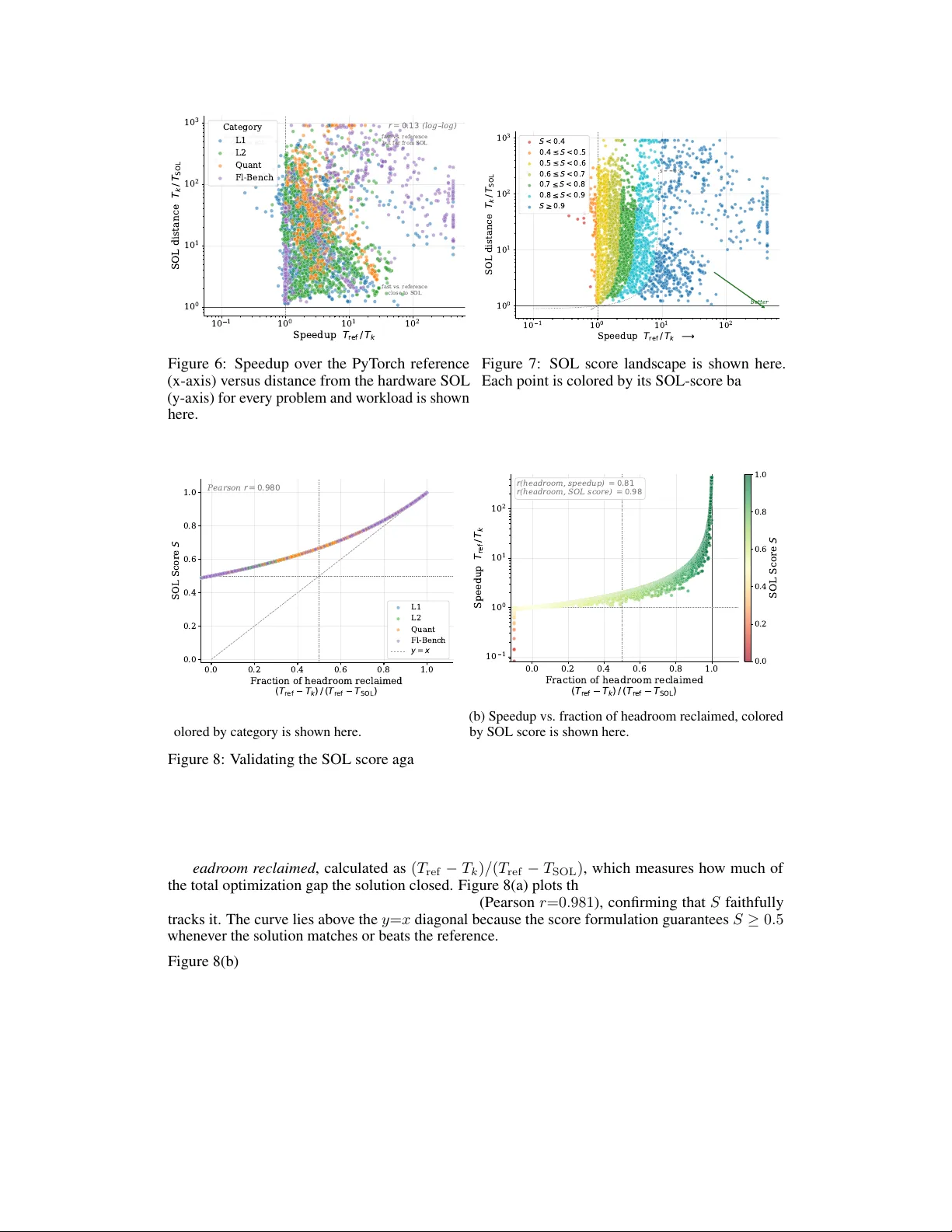
Original Paper
Loading high-quality paper...
Comments & Academic Discussion
Loading comments...
Leave a Comment