Decorated Local Systems and Character Varieties

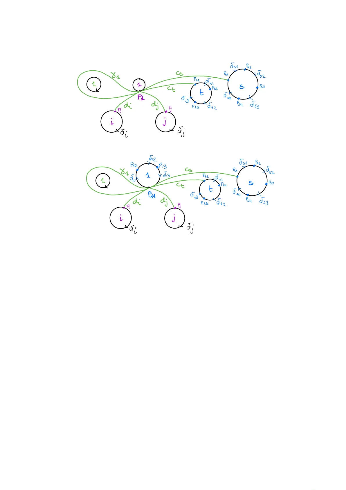
Decorated Local Systems and Character V arieties Benedetta F acciotti, Marta Mazzocco, Nikita Nikolaev March 20, 2026 Abstract The focus of this paper is the study of the moduli space of representations of fundamen- tal groupoids of surfaces Σ with boundaries with values in G := GL n ( C ) . In absence of marked points on the boundary , this moduli space is realized in many equivalent ways: as the moduli space of linear local systems on Σ , as the moduli space of representations of the fundamental groupoid Π 1 (Σ) , as the space of monodromy data and as character variety . By adding marked points to the boundary of Σ in order to capture irregular sin- gularities, the Betti moduli space has been generalized in several ways by many authors. Although it is clear that these different approaches describe essentially the same spaces of mathematical objects, exactly how they ﬁt together has not yet been established. Mo- tivated by the broader programme of establishing an explicit and conceptually coherent relationship between the existing approaches to the study of the decorated Betti moduli space, in this paper , we develop a categorical framework that allows for a systematic deﬁnition of the decorated Betti moduli spaces space, in the presence of higher order poles, designed to specialize to the different points of view encountered in the literature. Contents 1 R eview: Local Systems and Character V arieties 7 1.1 Groupoids and Moduli Spaces . . . . . . . . . . . . . . . . . . . . . . . . . . . . . . . . 7 1.2 Linear Local Systems . . . . . . . . . . . . . . . . . . . . . . . . . . . . . . . . . . . . . 8 1.3 Groupoid R epresentations and Holonomy . . . . . . . . . . . . . . . . . . . . . . . . . 11 1.4 Character V ariety . . . . . . . . . . . . . . . . . . . . . . . . . . . . . . . . . . . . . . . 15 1.5 Monodromy Data . . . . . . . . . . . . . . . . . . . . . . . . . . . . . . . . . . . . . . . 16 2 Surfaces with Marked Boundary 18 2.1 Discrete Fundamental Groupoid . . . . . . . . . . . . . . . . . . . . . . . . . . . . . . . 21 3 Decorated Local Systems 25 3.1 Filtered Local Systems . . . . . . . . . . . . . . . . . . . . . . . . . . . . . . . . . . . . 25 3.2 Framed Local Systems . . . . . . . . . . . . . . . . . . . . . . . . . . . . . . . . . . . . 27 3.3 Projectively Framed Local Systems . . . . . . . . . . . . . . . . . . . . . . . . . . . . . 30 4 Decorated Groupoid R epresentations 30 4.1 Filtered Groupoid Representations . . . . . . . . . . . . . . . . . . . . . . . . . . . . . 30 4.2 Framed and Projectively Framed Groupoid Representations . . . . . . . . . . . . . . . 32 4.3 Discrete and Decorated Groupoid Representations . . . . . . . . . . . . . . . . . . . . . 33 5 F orgetting secondary points 37 1 5.1 Stratiﬁcation by Relative P osition of Adjacent Flags . . . . . . . . . . . . . . . . . . . . 37 5.2 Invariant Flags and Shufﬂed Jordan T ype . . . . . . . . . . . . . . . . . . . . . . . . . . 39 5.3 F orgetful functors . . . . . . . . . . . . . . . . . . . . . . . . . . . . . . . . . . . . . . . 40 6 Decorated Character V arieties 41 6.1 Mixed Conjugation Action Groupoid . . . . . . . . . . . . . . . . . . . . . . . . . . . . 42 6.2 Decorated Representation V ariety . . . . . . . . . . . . . . . . . . . . . . . . . . . . . . 44 6.3 Filtered, Framed and Projectively Framed Character V arieties . . . . . . . . . . . . . . 47 6.4 Finite-Dimensional Presentation . . . . . . . . . . . . . . . . . . . . . . . . . . . . . . . 50 A Proof of Proposition 1.4 52 B Invariant Flags and Shufﬂed Jordan T ypes 57 B.1 Review of Linear Algebra and Jordan T ypes . . . . . . . . . . . . . . . . . . . . . . . . 59 B.2 Shufﬂed Jordan T ypes . . . . . . . . . . . . . . . . . . . . . . . . . . . . . . . . . . . . 61 B.3 Shufﬂed Jordan types from Jordan Basis . . . . . . . . . . . . . . . . . . . . . . . . . . 65 B.4 Invariant Flags as shufﬂed Jordan types . . . . . . . . . . . . . . . . . . . . . . . . . . 66 B.5 Shufﬂed Jordan Matrices . . . . . . . . . . . . . . . . . . . . . . . . . . . . . . . . . . . 67 B.6 B -Conjugacy Classes in B . . . . . . . . . . . . . . . . . . . . . . . . . . . . . . . . . . 70 R eferences 71 Introduction The focus of this paper is the study of moduli spaces of representations of fundamental groupoids of surfaces Σ with boundaries with values in G := GL n ( C ) . In absence of marked points on the boundary , this moduli space is realized in many equivalent ways: as the moduli space Loc G (Σ) of linear local systems on Σ , as the moduli space Rep G  Π 1 (Σ)  of represen- tations of the fundamental groupoid Π 1 (Σ) , as the moduli space Rep G  π 1 (Σ , p )  of mon- odromy data and as character variety X G (Σ) . W e call all these moduli spaces 1 collectively as Betti moduli space . Their equivalence can be stated as follows: Loc G (Σ) ∼ = Rep G  Π 1 (Σ)  ∼ = Rep G  π 1 (Σ , p )  ∼ = X G (Σ) . F or convenience of the reader , we recall these deﬁnitions and the proof of these equivalences in Sections 1.2, 1.3 and 1.4. By adding marked points to the boundary of Σ in order to capture irregular singularities, the Betti moduli space has been generalized in several ways by many authors as summarized below . Although it is clear that these different approaches describe essentially the same spaces of mathematical objects, exactly how they ﬁt together has not yet been established. In this paper , we develop a categorical framework that allows for a clear and systematic deﬁnition of the decorated Betti moduli spaces designed to specialize to the different points of view encountered in the literature. Let us brieﬂy recall the generalizations considered in this paper . 1 When we speak of a moduli space , we think of an appropriate moduli stack, but in almost every instance it is sufﬁcient to restrict our attention to the underlying set of isomorphism classes. 2 The moduli space of linear local systems was enriched by adding ﬁltrations at marked points implicitly in Deligne’s work on regular singular connections [Del70]. The systematic con- struction of moduli spaces of such ﬁltered local systems was later carried out by Simpson in the context of parabolic structures [Sim90], and further extended to irregular singularities by Boalch. Building on this framework, F ock and Goncharov study special positive and deco- rated loci inside these moduli spaces, endowing them with cluster structures and giving rise to higher T eichm ¨ uller spaces [FG06]. The notion of moduli space of ﬁltered 2 was further generalized by Goncharov and Shen [GS19] who introduced the moduli space of pinnings, namely an enrichment of the moduli space of ﬁltered G –local systems on Σ by adding dec- orations on some of the ﬂags. Note that the concept of pinning was essentially introduced by Chevalley and later formalised by T its, Grothendieck, and Demazure in the study of re- ductive algebraic groups. In the context of ﬁltered local systems, pinnings were used by F ock-Goncharov [FG06, §2.2] and Goncharov-Shen who gave an alternative deﬁnition of pinning [GS19, Def 3.7, fn. 12]. If the group is adjoint (e.g., PGL ( C ) but not GL n ( C ) ), then their deﬁnition of pinning is equivalent to the classical notion [GS19, Lemma 3.30]. The moduli space of representations of the fundamental groupoid was generalized by Gual- tieri, Li and Pym in [GLP18] exploting the theory of Lie groupoids and Lie algebroids which is naturally involved in the holomorphic case, in which the Betti moduli space is naturally homeomorphic to the de Rham moduli space of holomorphic connections on a Riemann sur- face. Indeed, any holomorphic connection on a Riemann surface Σ deﬁnes a representation of the space of vector ﬁelds T Σ , which has a structure of a Lie algebroid. A distinguished integration of such a Lie algebroid is the fundamental Lie groupoid Π 1 (Σ) , whose represen- tation corresponds to the parallel transport determined by the connection. By Lie’s second theorem, representations of T Σ and Π 1 (Σ) are equivalent. What they showed is that this construction can be naturally extended to the case of higher order poles by incorporating the effective divisor D encoding the poles and their multiplicities. Hence, as meromorphic connections are representations of the Lie algebroid T Σ ( − D ) of vector ﬁelds vanishing along D , Lie’s second theorem implies they are equivalent to representations of the integrating Lie groupoid Π 1 (Σ , D ) . The moduli space of monodromy data was generalized by Boalch in [Boa01], where he introduced a moduli space that was later called wild character variety in [Boa14]. T opologi- cally , instead of the original Riemann surface, one considers its real oriented blow-up at the poles of the connection. Additional points are then removed at the intersections of circles in tubular neighborhoods around the boundaries created by higher-order poles with the so- called Stokes directions. Algebraically , rather than using the usual notion of representation, the construction employs Stokes representations, deﬁned in [Boa01]. The moduli space is then deﬁned taking the quotient by a speciﬁc action of the centralizer of the irregular type deﬁned around each pole. 2 W e note that in [FG06] the authors use the term framed instead of ﬁltered. 3 Finally , in [CMR17], Chekhov , Mazzocco and R ubtsov deﬁned the so called decorated charac- ter variety , now renamed bordered cusped character variety . The construction of this moduli space involves some topological modiﬁcations to the starting surface, based on [GMN13]. More precisely , while one still needs to consider the real oriented blow-up of the surface at the poles, the approach here differs in that, instead of introducing additional punctures, one designates marked points on the boundaries arising from higher order poles only . T reat- ing the marked points as cusps, the authors assign a Borel subgroup to each of them. The bordered cusped character variety is then the quotient of the representation space of the groupoid of arcs with base points at the cusps by the action by mixed conjugation (see sub- section 6.1) of the unipotent radical of the Borel subgorups associated to the cusps. This approach was then generalized to the n dimensional case in [CMR18]. This paper is motivated by the broader programme of establishing an explicit and concep- tually coherent relationship between all the above existing approaches to the study of the decorated Betti moduli space. As a concrete contribution to this programme, we develop a categorical framework that allows for a systematic deﬁnition of the Betti moduli space in the presence of higher order poles. This viewpoint is also compatible with the Riemann–Hilbert correspondence, whose emphasis on the classiﬁcation of geometric and algebraic objects makes a categorical perspective natural. The ﬁrst key step of our approach is therefore the introduction of suitable groupoids that accurately describe these structures. In order to state the main result of this paper , we brieﬂy introduce the notation for the rele- vant groupoids by providing a rough description of their objects, referring the reader to the appropriate sections for the precise deﬁnitions. A common feature of all these groupoids is that their objects carry certain decorations on the ﬁbers/stalks over the marked points. In this paper , we consider surfaces with marked boundary (Σ , P ) , where Σ is a compact con- nected, oriented, smooth real two-dimensional manifold with boundary components each of which is diffeomorphic to a circle, and P ⊂ ∂ Σ is a ﬁnite set of points. These points carry some extra information as described in Deﬁnition 2.2, but we neglect it in this introduc- tion. F ollowing [FG06], a ﬁltered local system on a surface with marked boundary (Σ , P ) is a pair ( E , F ) consisting of a local system E on Σ endowed with a collection F = {F p : p ∈ P } where F p is a ﬁltration near p (see Deﬁnition 3.1). W e denote the groupoid of ﬁltered local systems, and the corresponding moduli space, respectively by Loc Fi G (Σ , P ) and Loc Fi G (Σ , P ) : = Loc Fi G (Σ , P )  ∼ . Next, a ﬁltered representation of the fundamental groupoid Π 1 (Σ) of a surface with marked boundary (Σ , P ) is a triple ( E , F, Φ) consisting of a representation ( E , Φ) of the fundamental groupoid Π 1 (Σ) endowed with a collection F : = { F p : p ∈ P } of ﬁltrations on the ﬁbres over 4 the marked points which are ﬂat in the sense speciﬁed in Deﬁnition 4.1. W e denote the groupoid of ﬁltered representations of rank n on (Σ , P ) with ﬁltered isomorphisms, and the corresponding moduli space (see Deﬁnition 4.2), by R ep Fi G  Π 1 (Σ) , P  and Rep Fi G  Π 1 (Σ) , P  : = R ep Fi G  Π 1 (Σ) , P  ∼ . Thanks to the fact that the decorations arise only on marked points, the introduction of a discrete model for this groupoid is natural. Therefore, we introduce the groupoid of ﬁltered representations of π 1 (Σ , P ) of rank n , and the corresponding moduli space (see Deﬁnitions 4.12 and 4.13) by R ep Fi G  π 1 (Σ , P )  and Rep Fi G  π 1 (Σ , P )  : = R ep Fi G  π 1 (Σ , P )  ∼ respectively . Finally we consider (see Deﬁnition 6.3) the decorated representation variety of (Σ , P ) , namely the subset R G (Σ , P ) of Hom  π 1 (Σ , P ) , G  consisting of all groupoid homomorphisms ρ : π 1 (Σ , P ) → G which are upper-triangular on loops based at marked points that lie on boundaries corresponding to simple poles. On this, we act by mixed conjugation by the afﬁne algebraic subgroup of G P := G | P | : B P : = Y p ∈ P B = Aut ( C n , C • ) where Aut ( C n , C • ) is the set of automorphisms of C n that preserve the standard ﬂag C • . In this way , we get an action groupoid on an afﬁne algebraic variety: B P ⋉ R G (Σ , P ) with g .ρ : = t ∗ g · ρ · s ∗ g − 1 . Its moduli space (see Deﬁnition 6.8) is called ﬁltered character stack and is deﬁned as the following afﬁne algebraic quotient stacks: X Fi G (Σ , P ) : = R G (Σ , P ) / B P . Similarly , we can introduce framed (and projectively framed) analogues of all the above cat- egories by framing every ﬂag with a basis (or the equivalence class of a basis) and requiring all ﬁltered isomorphisms to be unipotent (or projectively unipotent). W e denote the corre- sponding groupoids and moduli spaces in the same way as above replacing the index Fi by F r (or PF r ). Therefore we will speak of decorated groupoids when referring to both ﬁltered and framed (or projectively framed) groupoids. Establishing the equivalence of these groupoids yields, at the level of objects, a bijection between the underlying sets of the corresponding moduli spaces. 5 Theorem. F or any surface with marked boundary (Σ , P ) , there are canonical equivalences of categories between the groupoids of decorated local systems, decorated representations of the fundamental groupoid Π 1 (Σ) , decorated representations of the discrete fundamental groupoid π 1 (Σ , P ) , and suitable mixed conjugation action groupoids over the decorated representation variety R G (Σ , P ) : Loc □ G (Σ , P ) ∼ = R ep □ G  Π 1 (Σ) , P  ∼ = R ep □ G  π 1 (Σ , P )  ∼ = K □ P ⋉ R G (Σ , P ) , for any □ ∈ { Fi , F r , PF r } where K Fi P : = B P , K F r P : = U P and K F r P : = U × P (see (6.11) ). As a consequence, there are canonical bijections between the corresponding moduli sets:: Loc □ G (Σ , P ) ∼ = Rep □ G  Π 1 (Σ) , P  ∼ = Rep □ G  π 1 (Σ , P )  ∼ = X □ G (Σ , P ) . Since Loc Fi G (Σ , P ) carries a natural cluster variety structure [FG06], this theorem shows that this cluster structure is intrinsic to the ﬁltered Betti moduli space. In the case when all the boundaries coming from simple poles are unmarked, i.e. when P = P I (see Deﬁnition 2.2), and the group is SL n ( C ) , the framed character variety is of the form X F r SL n ( C ) (Σ , P I ) = Hom  π 1 (Σ , P I ) , SL n ( C )  / U P I . This was introduced by Chekhov , Mazzocco and R ubtsov in [CMR17, §4] (who called it the decorated character variety ) based on the work of Li-Bland and ˇ Severa in [L ˇ S15, §6]. These papers have served as one of the main inspirations for this project. In particular , we wanted to prove that the F ock-Goncharov- Shen variables can be used to coordinatize any of the above moduli sets even when some decorations are forgotten - see Remark 6.10. Motivated by this, in Section 5, we show that the map induced by the forgetful functor Loc Fi G (Σ , P ) − → Loc Fi G (Σ , P I ) is a ramiﬁed covering. This paper is organized as follows. In Section 1, we give a careful treatment of the classical setting of linear local systems on surfaces with boundary , representations of the fundamental groupoid, and the relationship between the corresponding character variety and the mod- uli space of monodromy data. In Section 2 we motivate and deﬁne surfaces with marked boundaries, and give a ﬁnite presentation for the fundamental groupoid π 1 (Σ , P ) . In Sec- tion 3, we introduce various notions of local systems, which we collectively call decorated local systems , and we discuss the relationships between them. In Section 4, we reformulate decorated local systems as decorated representations of the fundamental groupoid and the discrete fundamental groupoid. In Section 5, we study the forgetful functors that drop the secondary marked points. In Section 6, we give an explicit description of the moduli space of decorated local systems. 6 Acknowledgements The authors are grateful to Anton Alexseev , Marco Gualtieri, Gabriele R embado and V olodya R ubtsov for many discussions on the topics of this paper . This was funded by the Leverhulme T rust Research Project Grant RPG -2021-047 and by the Proyecto de Generaci ´ on de Conocimiento, PID2024-155686NB -I00 of the Spanish Ministry of Science, Innovation and Universities. 1 R eview: L ocal Systems and Character V arieties In this section, we set the stage by reviewing the classical setting of linear local systems on surfaces with boundary , representations of the fundamental groupoid, and the relationship between the corresponding character variety and the moduli space of monodromy data. W e give a rather careful treatment of the subject for the purpose of completeness as well as to introduce notation and recall basic concepts needed in the rest of the paper . In what follows, we put G : = GL n ( C ) for arbitrary n , and let B and U denote respectively the subgroups consisting of upper-triangular and unipotent upper-triangular matrices in G . W e also let Σ be any surface by which we mean a connected, oriented, topological real two-dimensional manifold with or without boundary . 1.1 Groupoids and Moduli Spaces 1.1.1 Groupoids First, recall that a groupoid is a category in which every morphism is invertible. T o spell this out a little, a groupoid consists of a set of objects X and a set of morphisms G together with several structure maps including a pair of maps s , t : G → X called the source and target maps which respectively extract the source and target objects of a morphism. W e usually say that G is a groupoid over X and write G ⇒ X . There is also an embedding of X into G as the subset of identity morphisms and we typically identify X with its embedded image inside G . A Lie groupoid is a groupoid G ⇒ X such that G and X are topological manifolds (although G may be non-Hausdorff), all the structure maps are continuous, the embedding X  → G is closed, and the source and target maps s , t are submersions. Similarly , we can deﬁne holomorphic and algebraic Lie groupoids. A groupoid homomorphism F : G → G ′ is simply a functor and a Lie groupoid homomorphism is a functor which is also a continuous (resp. holomorphic or algebraic) map. 1.1.2 Moduli spaces Any groupoid G ⇒ X has a corresponding moduli set : it is the set of isomorphism classes of objects in X that we shall denote in any of the following ways: G = X / G = X / ∼ . 7 If x is an object of X , we usually denote its isomorphism class by [ x ] . If the groupoid G ⇒ X carries additional structure — such as continuous, smooth, analytic, or algebraic — then the moduli set G may be enriched to a moduli stack in the respective category . However , these details will not play any appreciable role in our story . So, from now on, when we speak of a moduli space , we think of an appropriate moduli stack, but in almost every instance it is sufﬁcient to restrict our attention to the underlying moduli set. 1.1.3 Three examples of Lie groupoids The ﬁrst example of a Lie groupoid is as follows. If K × X → X is a group action on a set X , then we can form the action groupoid G = K ⋉ X ⇒ X . Its set of morphisms is given by K × X with source and target maps to X given by the natural projection and the group action, respectively: s( k , x ) = x and t( k , x ) = k .x . The composition is given by ( k 2 , x 2 ) ◦ ( k 1 , x 1 ) = ( k 2 k 1 , x 1 ) whenever x 2 = k 1 .x 1 . The corresponding moduli set X / K is the set of all K -orbits in X . Moreover , if X is an afﬁne algebraic variety , K is an afﬁne algebraic group, and the action is algebraic, then G = K ⋉ X ⇒ X is an algebraic Lie groupoid, and the corresponding moduli space G is an algebraic stack equal to the stack-theoretic quotient X / K . Second, the fundamental groupoid Π 1 (Σ) ⇒ Σ of the surface Σ is the space of all con- tinuous paths γ : [0 , 1] → X considered up to homotopy with ﬁxed endpoints. It is a real four-dimensional topological manifold. The restriction of the groupoid Π 1 (Σ) to a subset S ⊂ Σ is by deﬁnition the full subgroupoid Π 1 (Σ) | S : = s − 1 ( S ) ∩ t − 1 ( S ) ⊂ Π 1 (Σ) consisting of paths on Σ that begin and end in S . In particular , for any point p ∈ Σ , the restriction of the fundamental groupoid Π 1 (Σ) to p is nothing but the fundamental group: π 1 (Σ , p ) = Π 1 (Σ)   p = s − 1 ( p ) ∩ t − 1 ( p ) ⊂ Π 1 (Σ) . Thus, the fundamental group π 1 (Σ , p ) is an example of a groupoid over a single point. Third, to any topological complex vector bundle E → Σ , we can naturally associate a Lie groupoid GL ( E ) ⇒ Σ called the transport groupoid . Its objects are the points of Σ and its morphisms are the linear isomorphisms between the ﬁbres of E ; that is, for any pair of points p, q ∈ Σ , the set of morphisms in GL ( E ) from p to q is the set GL ( E | p , E | q ) of all linear isomorphisms E | p ∼ − → E | q . The restriction of GL ( E ) to a point p ∈ Σ is nothing but the automorphism group of the ﬁbre: GL ( E ) | p = GL ( E | p ) ≃ G . 1.2 Linear Local Systems In this paper , by a local system on Σ we shall mean either a linear local system or equiva- lently a G -local system. Let us quickly remind the reader of what these are and how to pass back and forth between the two notions. Linear local systems (more precisely , complex-linear local systems of ﬁnite rank ) are locally 8 constant sheaves E on Σ of ﬁnite-dimensional complex vector spaces. In particular , all stalks E p of E are complex vector spaces of the same dimension called the rank of E . Likewise, a G - local system is a locally constant sheaf ˆ E of sets on Σ equipped with a right G -action such that the stalk ˆ E p of ˆ E at every point p ∈ Σ is a G -torsor; i.e., a set equipped with a free and transitive right G -action. Linear local systems on Σ together with linear sheaf isomorphisms (i.e., sheaf morphisms which are linear isomorphisms on stalks) form a groupoid which, along with the corre- sponding moduli space of local systems , will be respectively denoted by Loc G (Σ) and Loc G (Σ) : = Loc G (Σ)  ∼ . W e usually draw no distinction between G -local systems and linear local systems because their categories are naturally equivalent thanks to the following lemma. Lemma 1.1. There is an equivalence of categories between the groupoid of linear local sys- tems and the groupoid of G -local systems (where morphisms are sheaf morphisms which are G -equivariant maps on stalks) given by the following pair of inverse functors: E 7− → ˆ E = GL ( C n , E ) and ˆ E 7− → E : = ˆ E × G C n Σ . The notation for this pair of functors will be explained in the course of the proof . Proof. If E is a linear local system of rank n , then for any p ∈ Σ the set ˆ E p : = GL ( C n , E p ) of all linear isomorphisms C n ∼ − → E p is a G -torsor: it has a free and transitive right G -action by pre-composition; i.e., f .g = f ◦ g for any f ∈ GL ( C n , E p ) and any g ∈ G = GL ( C n ) . Similarly , the set GL  C n , E ( U )) for any open set U ⊂ Σ has a right G -action though not necessarily free and transitive. Therefore, the correspondence ˆ E : U 7→ GL  C n , E ( U )) is a locally constant sheaf of sets with a right G -action whose stalk at any p ∈ Σ is the G - torsor ˆ E p = GL ( C n , E p ) . In other words, ˆ E is a G -local system, which we call ˆ E = : GL ( C n , E ) by a slight abuse of notation. Conversely , if ˆ E is a G -local system, then E : = ˆ E × G C n Σ is a linear local system on Σ , where C n Σ is the constant sheaf with value C n with its natural right G -action. Recall that in general, if X and Y are two sets equipped with a right G -action, then X × G Y (sometimes called the tensor product of G -sets ) is deﬁned as the quotient set X × Y / ∼ by the equivalence relation ( x.g , y ) ∼ ( x, y .g ) for all x ∈ X , y ∈ Y , and g ∈ G . Let us now explain how these constructions extend to morphisms, thus deﬁning a pair of functors. R ecall that any morphism of sheaves is completely determined on stalks. So a 9 morphism of linear local systems ϕ : E → E ′ induces a linear map on stalks ϕ p : E p → E ′ p which in turn induces a G -equivariant map ˆ ϕ p : GL ( C n , E p ) → GL ( C n , E ′ p ) given by post- composition with ϕ p (i.e., f 7→ ϕ p ◦ f ), which in turn induces a sheaf morphism ˆ ϕ : GL ( C n , E ) → GL ( C n , E ′ ) ; i.e., ˆ ϕ : ˆ E → ˆ E ′ . Conversely , any morphism of G -local systems ˆ ϕ : ˆ E → ˆ E ′ induces a G -equivariant map on stalks ˆ ϕ p : ˆ E p → ˆ E ′ p which in turn induces a linear map ϕ p : ˆ E p × G C n → ˆ E ′ p × G C n given by ( f , v ) 7→  ˆ ϕ p ( f ) , v  and therefore a linear morphism ϕ : E → E ′ . T o see that ϕ p is indeed a linear map, recall that ˆ E ′ p is a G -torsor , so for any f ∈ ˆ E p there is a unique element g ∈ G such that ˆ ϕ p ( f ) = f .g = f ◦ g , and so  ˆ ϕ p ( f ) , v  = ( f .g , v ) ∼ ( f , v g ) . Finally , we explain why these two functors determine an equivalence of categories. F or the sake of lighter notations, let us denote by C and D the categories of linear local systems on Σ and the one of G -local systems on Σ respectively , by F and G the functors F : C 7− → D and G : D 7− → C . If E is a linear local system and ˆ E = GL ( C n , E ) is the associated G -local system, then the associated linear local system E ′ : = ˆ E × G C n Σ is canonically isomorphic to E . The reason is that, at any p ∈ Σ , the stalk E ′ p = ˆ E p × G C n = GL ( C n , E p ) × G C n is canonically isomor- phic to E p because, for any n -dimensional vector space E , there is a canonical isomorphism GL ( C n , E ) × G C n ∼ − → E given by ( f , v ) 7→ f ( v ) . This isomorphism provides natural transformations η : Id C ⇒ G ◦ F and ζ : Id D ⇒ F ◦ G . Finally , we also mention that any diffeomorphism f : Σ ′ → Σ — or , more generally , any homotopy equivalence — induces an equivalence f ∗ : Loc G (Σ) ∼ − → Loc G (Σ ′ ) by pullback. In particular , any local system on Σ restricts to a local system on the interior Σ ◦ ⊂ Σ , and this restriction functor is actually an equivalence of categories Loc G (Σ) ∼ − → Loc G (Σ ◦ ) which has a canonical inverse. Lemma 1.2. F or any surface Σ , any local system E ◦ on the interior Σ ◦ has a canonical extension to a local system E on Σ , thus yielding an inverse pair of restriction-extension functors: Loc G (Σ) ∼ ⇌ Loc G (Σ ◦ ) . Proof. The canonical extension E to Σ of a local system E ◦ on Σ ◦ is deﬁned as follows. F or every boundary point p ∈ ∂ Σ , the stalk E p of E at p is deﬁned as the restriction of E ◦ to the germ of a sectorial neighbourhood of p . Recall that, since Σ is a manifold with boundary , a sectorial neighbourhood of a boundary point p is the intersection with Σ ◦ of a simply connected open boundary chart containing p . More precisely , E p : = lim − → E ◦ ( U ) is the direct limit of vector spaces E ◦ ( U ) indexed over all sectorial neighbourhoods U ⊂ Σ of p . Notice that since E ◦ is locally constant, the vector spaces E ◦ ( U ) stabilise in this limit, and so 10 there is a canonical linear isomorphism E p ∼ − → E ◦ ( U ) for any sectorial neighbourhood U of p . 1.3 Groupoid R epresentations and Holonomy A representation of a groupoid G ⇒ X is by deﬁnition a pair ( E , Φ) consisting of a complex vector bundle E → X and a groupoid morphism Φ : G → GL ( E ) . W e usually write Φ γ : = Φ( γ ) ∈ GL ( E ) for any γ ∈ G . A morphism ϕ : ( E , Φ) → ( E ′ , Φ ′ ) is a bundle map ϕ : E → E ′ which intertwines the homomorphisms Φ , Φ ′ in the following sense. F or any γ ∈ G with source and target p, q ∈ X , we have the following commutative diagram of maps between the ﬁbres of E and E ′ : E p E q E ′ p E ′ q Φ γ φ p φ q Φ ′ γ i.e. ϕ q ◦ Φ γ = Φ ′ γ ◦ ϕ p . (1.1) Moreover , if G is a topological (resp. smooth, holomorphic, algebraic) Lie groupoid, then the vector bundles E and the bundle maps ϕ are required to be continuous (resp. smooth, holomorphic, algebraic). W e denote the groupoid of representations of G ⇒ X of rank n and the corresponding moduli space by R ep G ( G ) and Rep G ( G ) : = R ep G ( G )  ∼ . In the case of the fundamental groupoid, we give the following Deﬁnition 1.3. A representation (or , more precisely , a linear representation of rank n , or a G -representation ) of the fundamental groupoid Π 1 (Σ) ⇒ Σ is a pair ( E , Φ) consisting of a topological complex vector bundle E → Σ of rank n and a (continuous) groupoid homomor- phism Φ : Π 1 (Σ) → GL ( E ) . Likewise, since the fundamental group is a groupoid over a single point and a vector bundle over a single point is a vector space, we recover representations of the fundamental group as groupoid representations. Recall that, given a point p ∈ Σ , a representation of the fundamental group π 1 (Σ , p ) is a pair ( E , φ ) consisting of an n -dimensional complex vector space E and a group homomorphism φ : π 1 (Σ , p ) → GL ( E ) . Since the fundamental group π 1 (Σ , p ) is the restriction of the fundamental groupoid Π 1 (Σ) to the point p , any representation ( E , Φ) of Π 1 (Σ) restricts to a representation of π 1 (Σ , p ) by taking E to be the ﬁbre E p of E at p and φ to be the restriction of Φ . This yields a restriction functor on representations: R : R ep G  Π 1 (Σ)  → R ep G  π 1 (Σ , p )  11 sending ( E , Φ) 7→ ( E , φ ) : =  E p , Φ   π 1 (Σ ,p )  . This functor turns out to be an equivalence of categories with a preferred explicit inverse equivalence that gives a convenient way to extend representations from the fundamental group π 1 (Σ , p ) to the fundamental groupoid Π 1 (Σ) . W e will state and prove this equivalence as part of a more general result (Proposition 1.4) after discussing the holonomy representa- tion. 1.3.1 Holonomy representation Any local system E on Σ induces a representation ( E , Φ) of the fundamental groupoid Π 1 (Σ) by taking the holonomy along paths, and vice versa by taking the deck-transformation- equivariant sections of a constant sheaf on the universal cover of Σ . Let us brieﬂy recall how this works. The holonomy of a local system E along a path γ : [0 , 1] → Σ from p to q ∈ Σ is by deﬁnition the linear isomorphism between on stalks, hol γ : E p ∼ − → E q , (1.2) deﬁned as the composition of canonical isomorphisms E p ∼ − → γ − 1 E  [0 , 1]  ∼ − → E q . When p = q , the isomorphism hol γ is usually called the monodromy of E along a loop γ based at p and denoted by mon γ . The isomorphisms deﬁning hol γ depend only on the homo- topy class of γ relative its endpoint and they exist by virtue of the fact that the inverse-image sheaf γ − 1 E on the interval [0 , 1] is constant because the interval is contractible. Further- more, observe that any sheaf morphism ϕ : E → E ′ deﬁnes a linear map γ − 1 E  [0 , 1]  → γ − 1 E ′  [0 , 1]  , and therefore the holonomies of E and E ′ along any path γ from p to q are related by the commutative diagram E p E q E ′ p E ′ q . hol γ φ p φ q hol ′ γ (1.3) Given a local system E , let O Σ be the sheaf of continuous functions on Σ and consider the vector bundle E : = E ⊗ O Σ (where, in line with common practice, we treat vector bundles interchangeably with their sheaves of sections). The ﬁbre E p of this bundle at any point p ∈ Σ is canonically isomorphic to the stalk E p . Then the holonomy of E deﬁnes a groupoid 12 homomorphism hol : Π 1 (Σ) → GL ( E ) sending γ 7→ hol γ . The result is a representation ( E , Φ) : = ( E ⊗ O Σ , hol) of the fundamental groupoid Π 1 (Σ) called the holonomy representation of E . If, in addition, we ﬁx a basepoint p ∈ Σ , then the restriction of the holonomy representation of E to the fundamental group π 1 (Σ , p ) deter- mines a representation ( E , Φ) : = ( E p , mon p ) with mon p : π 1 (Σ , p ) → GL ( E p ) sending γ 7→ mon γ called the monodromy representation of E at p . Proposition 1.4. There is an equivalence of categories Hol : Loc G (Σ) ∼ − → R ep G  Π 1 (Σ)  sending E 7− → ( E , Φ) : = ( E ⊗ O Σ , hol) called the holonomy representation functor which associates a local system to its holonomy representation. Furthermore, for any p ∈ Σ , the composition of the restriction functor with the holonomy representation functor is an equivalence of categories Mon p : Loc G (Σ) ∼ − → R ep G  π 1 (Σ , p )  sending E 7− → ( E , φ ) : = ( E p , mon p ) called the monodromy representation functor . Consequently , the restriction of represen- tations from the fundamental groupoid Π 1 (Σ) to the fundamental group π 1 (Σ , p ) is also an equivalence of categories: R : R ep G  Π 1 (Σ)  ∼ − → R ep G  π 1 (Σ , p )  sending ( E , Φ) 7→ ( E , φ ) : =  E p , Φ   π 1 (Σ ,p )  . Explicitly , an inverse to the monodromy representation functor Mon p is given by Mon − 1 p : ( E , φ ) 7→ E : =  ˜ Σ × E  /π 1 (Σ , p ) where ˜ Σ → Σ is the universal cover based at p and the quotient is by the diagonal action of π 1 (Σ , p ) by deck transformations on ˜ Σ and by the representation φ on E . Similarly , an inverse functor to the restriction functor R lifts a representation ( E , φ ) of π 1 (Σ , p ) to the holonomy 13 representation of the local system E =  ˜ Σ × E  /π 1 (Σ , p ) ; i.e., R − 1 : = Hol ◦ Mon − 1 p . These notations will be fully explained in the course of the proof (speciﬁcally , see (A.1)) of this classical result. F or clarity , we remark that the holonomy and monodromy representation functors ﬁt into the commutative diagram Loc G (Σ) R ep G  Π 1 (Σ)  R ep G  π 1 (Σ , p )  . Hol Mon p R W e also state the following immediate corollary of Proposition 1.4. Corollary 1.5. There are canonical bijections between the moduli spaces of local systems, of representations of the fundamental groupoid Π 1 (Σ) , and of representations of the fundamental group π 1 (Σ , p ) for any p ∈ Σ : Loc G (Σ) ∼ = Rep G  Π 1 (Σ)  ∼ = Rep G  π 1 (Σ , p )  , given by [ E ] 7→ [Hol( E )] 7→ [Mon p ( E )] . Although Proposition 1.4 is classical, we have found no single reference that cleanly ad- dresses all of its aspects. F or this reason, and because we shall use parts of this proof in the next section, we supply a detailed proof in Appendix A. R emark 1.6. Let us explain in more detail the deﬁnition (1.2) of the holonomy of a local system E along a path γ . First, the inverse image γ − 1 E is by deﬁnition the sheaf on the interval [0 , 1] associated with the presheaf that sends open subsets I ⊂ [0 , 1] to the direct limit of E ( U ) over open subsets U ⊂ Σ containing the image γ (I) ; in symbols, I 7→ lim − → E ( U ) . Concretely , this implies that for any open subset I ⊂ [0 , 1] , there is an open neighbourhood U ⊂ Σ of γ (I) together with a linear map E ( U ) → γ − 1 E (I) . Since E is locally constant, it follows that the inverse image sheaf γ − 1 E is locally constant, too: for any sufﬁciently small open subset I ⊂ [0 , 1] , there is an open neighbourhood U of γ (I) such that the restriction E | U is a constant sheaf on U , which implies that the restriction γ − 1 E   I is a constant sheaf on I with a canonical isomorphism E ( U ) ∼ − → γ − 1 E (I) . But since [0 , 1] is contractible, the locally constant sheaf γ − 1 E is in fact a constant sheaf on [0 , 1] , which means means there is a canonical isomorphism γ − 1 E (I) ∼ − → γ − 1 E  [0 , 1]  for any open subset I ⊂ [0 , 1] . Next, any half-open interval [0 ,  ) is an open subset of [0 , 1] , so any open neighbourhood U of the image γ  [0 ,  )  is in particular an open neighbourhood of p = γ (0) . But since E p is the stalk of the locally constant sheaf E at p , there is by deﬁnition an isomorphism 14 E p ∼ − → E ( U ) for a sufﬁciently small U . Consequently , we ﬁnd the canonical isomorphism E p ∼ − → γ − 1 E  [0 , 1]  used in the deﬁnition of the holonomy hol γ . ◦ 1.4 Character V ariety The advantage of ﬁxing a point p ∈ Σ and reducing our attention to the representations of the fundamental group π 1 (Σ , p ) is that it can be used to give an explicit, ﬁnite-dimensional model of the moduli space Loc G (Σ) . A frame (or framing ) on an n -dimensional vector space E is an isomorphism β : E ∼ − → C n . Equivalently , a frame is a choice of an ordered basis of E or of a group isomorphism GL ( E ) ∼ − → G . Therefore, given any representation ( E , Φ) of π 1 (Σ , p ) , a frame on E induces a group homomorphism ρ : π 1 (Σ , p ) → G deﬁned by ρ : γ 7→ ρ γ : = β ◦ Φ γ ◦ β − 1 . Conversely , any ρ : π 1 (Σ , p ) → G gives rise to the representation ( C n , ρ ) . If ( E , Φ) is a representation with frame β , then changing the frame on E has the effect of conjugating the homomorphism ρ by an element of G . Namely , ρ ′ : γ 7→ ρ ′ γ = g ρ γ g − 1 whenever β ′ ◦ β − 1 = g ∈ G . This formula deﬁnes a conjugation action of G on the set of group homomorphisms, called the representation variety , R G (Σ , p ) : = Hom  π 1 (Σ , p ) , G  . Likewise, if ϕ : ( E , Φ) ∼ − → ( E ′ , Φ ′ ) is an isomorphism and β , β ′ are frames on E , E ′ that determine ρ, ρ ′ ∈ R G (Σ , p ) , then ϕ gives a group element g : = β ′ ◦ ϕ ◦ β − 1 ∈ G which relates ρ and ρ by the same conjugation action: ρ ′ γ = g ρ γ g − 1 for all γ ∈ π 1 (Σ , p ) . This deﬁnes an inclusion functor from the action groupoid G ⋉ R G (Σ , p ) to the groupoid of representations of π 1 (Σ , p ) , and this functor turns out to be an equivalence. Proposition 1.7. There is a canonical equivalence of categories R ep G  π 1 (Σ , p )  ∼ = G ⋉ R G (Σ , p ) . Furthermore, for any p, p ′ ∈ Σ , there is an equivalence of categories G ⋉ R G (Σ , p ) ∼ = G ⋉ R G (Σ , p ′ ) . This equivalence is given by the inclusion functor G ⋉ R G (Σ , p ) ∼ − → R ep G  π 1 (Σ , p )  sending ρ 7− → ( E , Φ) : = ( C n , ρ ) , and viewing any g ∈ G as an isomorphism g : C n → C n . An inverse functor requires a choice of frame β : E ∼ − → C n for every vector space E ∈ V ec G . Once chosen, it is given on objects by ( E , Φ) 7→ ρ where ρ γ : = β ◦ Φ γ ◦ β − 1 for all γ ∈ π 1 (Σ , p ) , and on morphisms by ϕ 7→ g : = β ′ ◦ ϕ ◦ β − 1 . 15 Proof of Proposition 1.7. W e just need to check that any inverse functor deﬁned as suggested above is indeed inverse to the inclusion functor . That it is a left inverse is obvious especially if we choose the identity frame on C n . F or a right inverse, if ( E , Φ) 7→ ρ via a frame β , then β in fact deﬁnes the desired isomorphism from ( E , Φ) to ( C n , ρ ) . If Σ is compact, the representation variety R G (Σ , p ) is a smooth afﬁne algebraic variety [RBC96; Sik12]. If Σ has genus g and no boundary , then the representation variety has dimension n 2 (2 g − 1) + 1 when g ≥ 2 and ( n 2 + n ) g when g = 0 , 1 . If Σ has s ≥ 1 holes then the representation variety has dimension n 2 (2 g + s − 1) . The afﬁne algebraic group G is acting algebraically on the afﬁne algebraic variety R G (Σ , p ) , so the action groupoid G ⋉ R G (Σ , p ) is algebraic. Its moduli space is the well-known algebraic quotient stack called the character variety : X G (Σ) : = R G (Σ , p )  G . Corollary 1.8. There are canonical bijections between the moduli spaces of local systems, rep- resentations of the fundamental groupoid Π 1 (Σ) , representations of the fundamental group π 1 (Σ , p ) for any basepoint p ∈ Σ , and the character stack of Σ : Loc G (Σ) ∼ = Rep G  Π 1 (Σ)  ∼ = Rep G  π 1 (Σ , p )  ∼ = X G (Σ) . Consequently , all these moduli spaces have a natural structure of an afﬁne algebraic quotient stack. Explicitly , the above bijection is deﬁned as the composition Loc G (Σ) → Rep G  π 1 (Σ , p )  → Hom  π 1 (Σ , p ) , G ) / G = X G (Σ) [ E ] 7→ [Mon p ( E )] = [( E p , mon p )] 7→ [ ρ ] where the last arrow involves choosing a frame on the vector space E p . 1.5 Monodromy Data Finally , if Σ is compact of genus g , then it has at most ﬁnitely many boundary components. Then the fundamental group π 1 (Σ , p ) is ﬁnitely generated by 2 g + s generators with one relation, where s ≥ 0 is the total number of punctures and boundary components of Σ , collectively referred to as holes . In fact, if there is at least one hole (i.e., s ≥ 1 ), then π 1 (Σ , p ) is a free group on 2 g + s − 1 generators. A generating set can be obtained by selecting s loops going round the holes of Σ as well as 2 g loops representing the A and B -cycles. More precisely: 1. Choose any collection of 2 g oriented loops α 1 , . . . , α g , β 1 , . . . , β g based at p that deter- 16 mine a basis of A and B -cycles. Namely , if Σ ′ denotes the closed surface obtained from Σ by capping off all boundary components, then the fundamental group π 1 (Σ ′ , p ) is generated by the α i , β i such that Q g i =1 [ α i , β i ] = 1 where [ α i , β i ] : = α i β i α − 1 i β − 1 i is the commutator and 1 = 1 p is the constant path at p . 2. If s ≥ 1 , enumerate all holes of Σ as 1 , . . . , s . F or each i = 1 , . . . , s , let γ i be a positively- oriented loop based at p going round only the i -th hole; i.e., γ i belongs to the conjugacy class in π 1 (Σ , p ) determined by the i -th hole. These generators can be chosen in such a way as to satisfy the relation g ← − Y i =1 [ α i , β i ] s ← − Y i =1 γ i = 1 . (1.4) Here, the left arrow over the product sign indicates that the product is taken from right to left. Therefore, the fundamental group has an explicit presentation π 1 (Σ , p ) ∼ =  α i , β i , γ i   relation (1.4)  . (1.5) The relation (1.4) can be solved for any γ i , but not for any of the α i or β i . Consequently , if s ≥ 1 , then π 1 (Σ , p ) is isomorphic to the free group on 2 g + s − 1 generators. Next, we introduce the following deﬁnition. Deﬁnition 1.9. F or any integers g , s ≥ 0 , a monodromy data in G of type ( g , s ) is any collection of matrices ( A , B , M ) ⊂ G consisting of: • A : = { A 1 , . . . , A g } , B : = { B 1 , . . . , B g } called period monodromies ; • M : = { M 1 , . . . , M s } called standard monodromies ; and satisfying the following relation: g ← − Y i =1 [ A i , B i ] s ← − Y i =1 M i = 1 . (1.6) W e denote the space of monodromy data in G of type ( g , s ) by Mon G ( g , s ) : = n ( A , B , M ) ∈ G 2g + s    relation (1.6) o . Deﬁnition 1.10. T o equip a surface Σ of genus g with s holes with monodromy data is to choose a point p ∈ Σ and an isomorphism R G (Σ , p ) ∼ − → Mon G ( g , s ) . 17 A choice of ﬁnite presentation of the fundamental group π 1 (Σ , p ) of the form (1.5) determines such an isomorphism by associating monodromy data ( A , B , M ) ∈ Mon G ( g , s ) to the genera- tors ( α , β , γ ) of π 1 (Σ , p ) like so: α i 7→ A i , β i 7→ B i , γ i 7→ M i . Note that if s ≥ 1 , then by eliminating one of the matrices M i from the list ( A , B , M ) of generators destroys the relation (1.6). This yields a bijection Mon G ( g , s ) ∼ = G 2g + s − 1 which shows that the set of monodromy data Mon G ( g , s ) is a smooth afﬁne algebraic variety of dimension (2 g + s − 1) n 2 provided that s ≥ 1 . The space of monodromy data Mon G ( g , s ) is equipped with a natural left G -action given by simultaneous conjugation: g . ( A , B , M ) = ( g A g − 1 , g B g − 1 , g M g − 1 ) . Then we arrive at the following classical result. Proposition 1.11. Let Σ be a surface of genus g with s holes. Then there is a non-canonical equivalence of categories between the groupoid of G -local systems on Σ and an action groupoid over the space of monodromy data of type ( g , s ) : Loc G (Σ) ≃ G ⋉ Mon G ( g , s ) . T o obtain such an equivalence, ﬁx a point p ∈ Σ and choose any presentation of the fundamental group π 1 (Σ , p ) of the form (1.5) . Consequently , there is a bijection between the character variety and the moduli space of monodromy data: X G (Σ) ∼ = Mon G ( g , s ) / G . In particular , if s ≥ 1 , then X G (Σ) ∼ = G 2 g + s − 1 / G . Consequently , the moduli space Loc G (Σ) of G - local systems on Σ is an algebraic stack of dimension (2 g − 2) n 2 + 2 if s = 0 and (2 g + s − 2) n 2 + 1 if s ≥ 1 . W e stress that the above equivalence and bijection depend nontrivially on the chosen pre- sentation (1.5) of π 1 (Σ , p ) . 2 Surfaces with Marked Boundary R ecall that a bordered surface is a connected, oriented, smooth real two-dimensional manifold- with-boundary Σ which we also assume to be compact. It has ﬁnitely many boundary com- ponents each of which is diffeomorphic to a circle. A marked bordered surface is a pair consisting of a bordered surface equipped with a ﬁnite nonempty subset of marked points 18 such that each boundary component contains at least one marked point. An isomorphism of marked bordered surfaces is an orientation-preserving diffeomorphism that sends marked points to marked points. R emark 2.1. The terminology for marked bordered surfaces matches what seems to be a broadly accepted meaning in the literature, including F omin-Shapiro-Thurston [FST08, §2], Smith [Smi15], Bridgeland-Smith [B S15, §8], Allegretti-Bridgeland [AB20, §3.6], Allegretti [All21, §2], to name a few . However , it corresponds to what Goncharov [Gon17, §1] and Goncharov-Shen [GS19, §2] call a “decorated surface”. ◦ Marked points in the interior are called punctures . F or our purposes, it will be more natural to work not with marked bordered surfaces but with their real-oriented blowups along the punctures. Concretely , the real-oriented blowup (see, e.g., [Nik24, §1.1]) of any marked bordered surface is a bordered surface Σ obtained by replacing each puncture with a bound- ary circle containing no marked points whilst keeping the rest of the surface, including the boundary marked points, unchanged. Thus, Σ has marked points on some, but not all, boundary components. Furthermore, sometimes it will be important for us to place an extra marked point on each unmarked boundary of Σ yet still be able to distinguish the original boundary circles with marked points from the ones that arose from punctures. This moti- vates the following deﬁnition. Deﬁnition 2.2. A surface with marked boundary is a pair (Σ , P ) where Σ is a compact bordered surface whose boundary components are partitioned as I = I sim ⊔ I reg ⊔ I irr into simple , regular , and irregular boundary circles, and where P ⊂ ∂ Σ is a ﬁnite set of boundary marked points , itself partitioned as P = P I ⊔ P II into respectively primary marked points and secondary marked points . Furthermore, every irregular boundary circle contains at least one primary marked point and no regular ones; every regular boundary circle contains exactly one secondary marked point and no primary ones; and every simple boundary circle contains no marked points at all. An isomorphism f : (Σ , P ) → (Σ ′ , P ′ ) of decorated surfaces is an orientation-preserving homeomorphism f : Σ → Σ ′ with the property that f ( P I ) = P ′ I and f ( P II ) = P ′ II . Often only the relative position of the marked points plays any role. So for almost everything we say , we may allow the subset P ⊂ ∂ Σ to be deﬁned only up to isotopy , which concretely means that marked points can slide continuously along the boundary without crossing each other . Hence, secondary marked points, being the sole occupiers of a regular boundary circle, are free to move around unconstrained. R emark 2.3. F ock-Goncharov [FG06, Def 1.1] use the term “marked surface” which in our 19 language is a surface with marked boundary in which all boundaries are marked. F ock-Rosly [FR99, §2] and F ock-Goncharov [FG07, §2] also use the terms “ciliated surface”, “cilia”, and “holes” which in our language mean respectively a surface with marked boundary with no secondary points, P II = ∅ , primary marked points , and simple boundary circles . Chekhov-Mazzocco [CM18], Chekhov-Mazzocco-R ubtsov [CMR18; CMR17], and Dal Martello- Mazzocco [DM24] use the terms “bordered cusped Riemann surface” or “Riemann surface with bordered” or “boundary cusps” for a manifold Σ g ,s,n whose underlying topological sur- face is in our language a surface with marked boundary with at least one primary marked point, P I  = ∅ and no secondary ones P II = ∅ . Boalch [Boa21] considers a smooth compact complex curve Σ with a ﬁnite subset a ⊂ Σ (using his notation). He then considers its real-oriented blowup ˆ Σ → Σ and decorates its boundary ∂ ˆ Σ with two types of marked points called “singular directions” A ⊂ ∂ ˆ Σ and “Stokes directions” S ⊂ ∂ ˆ Σ . If we drop the complex structure on ˆ Σ and consider just the underlying topological surface, then the pair ( ˆ Σ , A ) is an example of our surface with marked boundary with no secondary marked points. Jordan-Le-Schrader-Shapiro [JLSS21, Def 1.1] use the term “decorated surface” in a quite different way but which can be directly related to ours. Namely , their notion involves regions in Σ separated by simple curves, called “walls”, that are closed or have endpoints on the boundary . Their attention is largely restricted to a subclass called simple decorated surfaces [JLSS21, R em 1.5] which are equivalent to our our surface with marked boundary where all boundaries are marked. ◦ The boundary loop based at a marked point p ∈ P is the loop determined by the boundary circle containing p , oriented according to the natural orientation on the boundary ∂ Σ . W e also consider the punctured boundary ˆ ∂ Σ : = ∂ Σ ∖ P I , punctured along the primary marked points only . It is a union of circles and open intervals. A boundary segment δ ⊂ ∂ Σ is the closure of a simply connected component of the punctured boundary ˆ ∂ Σ . It has a natural orientation matching the orientation of the boundary ∂ Σ . Thus, it is a path δ : [0 , 1] → ∂ Σ completely determined by its endpoints which are two (not necessarily distinct) primary marked points p 1 = δ (0) and p 2 = δ (1) ∈ P I . F or this reason, we may sometimes denote this boundary segment using the interval notation [ p 1 , p 2 ] . W e denote the set of all boundary segments of (Σ , P ) by A = A (Σ , P ) : = { δ boundary segments } . R emark 2.4. Note that Goncharov-Shen introduce the term “coloured decorated surface” which in our language corresponds to a triple (Σ , P , A 0 ) consisting of a surface with marked 20 boundary (Σ , P ) and a sub-collection A 0 ⊂ A of boundary segments (which they call “coloured boundary intervals”). ◦ A surface with marked boundary (Σ , P ) is completely determined up to isomorphism by the genus g of Σ ; an ordered collection s : = ( l, r, d ) of non-negative integers equal respectively to the number of unmarked, marked by secondary points, and marked by primary points boundaries; and an unordered collection m : = { m 1 , . . . , m d } of strictly positive integers equal to the number of primary marked points per boundary circle marked by primary points. In total, (Σ , P ) has s = | s | : = l + r + d holes, r secondary marked points, m = | m | : = m 1 + . . . + m d primary marked points. Also, | P | = m + r . These considerations justify the following Deﬁnition 2.5. A surface with marked boundary (Σ , P ) is called of type ( g , s , m ) , where s : = ( l, r, d ) and m : = ( m 1 , . . . , m d ) , if it has l simple boundaries, r regular boundaries, d irregular boundaries and m i primary marked points on the i -th irregular boundary . 2.1 Discrete F undamental Groupoid Now , let (Σ , P ) be a surface with marked boundary such that P  = ∅ . Deﬁnition 2.6. The discrete fundamental groupoid of a surface with marked boundary (Σ , P ) is the restriction of the fundamental groupoid Π 1 (Σ) to P : π 1 (Σ , P ) : = Π 1 (Σ)   P = s − 1 ( P ) ∩ t − 1 ( P ) ⊂ Π 1 (Σ) . Note that the restricted fundamental groupoid Π 1 (Σ)   P : = s − 1 ( P ) ∩ t − 1 ( P ) makes sense as a groupoid over any subset P ⊂ Σ , not necessarily ﬁnite. However , our interest lies with surfaces with marked boundary: the upshot is that, just as every surface has a naturally associated continuous fundamental groupoid, every surface with marked boundary has a naturally associated discrete fundamental groupoid. W e call π 1 (Σ , P ) discrete because, in contrast to the continuous fundamental groupoid Π 1 (Σ) , it has ﬁnitely many objects P and any two objects are related by a countable collection of arrows. More accurately , the subspace topology on π 1 (Σ , P ) inherited from Π 1 (Σ) is the discrete topology . Even more importantly , as we argue next, the discrete fundamental groupoid π 1 (Σ , P ) is a ﬁnitely -generated groupoid , which means we can ﬁnd a ﬁnite collection of paths γ i ∈ π 1 (Σ , P ) such that any path γ ∈ π 1 (Σ , P ) can be written as a ﬁnite composition of the γ i . R emark 2.7. The discrete fundamental groupoid π 1 (Σ , P ) has been considered by Li–Bland- ˇ Severa [L ˇ S15, §4] who denoted it by Π 1 (Σ , V ) , and by Chekhov-Mazzocco-R ubtsov [CMR17, §4] who called it the “fundamental groupoid of arcs” and denoted it by U . It also appears in Dal Martello-Mazzocco [DM24, §3] who denote it by π a (Σ g ,s,m ) . ◦ Lemma 2.8. F or surface with marked boundary (Σ , P ) , where Σ has genus g and s holes, 21 the discrete fundamental groupoid π 1 (Σ , P ) is ﬁnitely generated by 2 g + s + | P | − 1 elements and one relation. Moreover , if s ≥ 1 , then π 1 (Σ , P ) is freely generated by 2 g + s + | P | − 2 elements. Any choice of such free generators determines (up to isotopy) a graph Γ embedded into Σ with vertices P such that the discrete fundamental groupoid π 1 (Σ , P ) is isomorphic to the free groupoid ΠΓ ⇒ P generated by Γ . Proof. Select any point p 0 ∈ P . R ecall that the fundamental group π 1 (Σ , p 0 ) is ﬁnitely gen- erated by 2 g + s elements satisfying one relation, and that it is in fact isomorphic to the free group on 2 g + s − 1 generators whenever s ≥ 1 . Let us take any such generating set. Next, for every point p ∈ P ∖ p 0 , choose a path from p 0 to p 1 . There are a total of | P | − 1 such paths. Then the resulting collection generates π 1 (Σ , P ) and satisﬁes one relation. 2.1.1 Finite Presentation W e now give a step-by-step prescription of choosing a convenient ﬁnite generating set for the discrete fundamental groupoid π 1 (Σ , P ) of any surface with marked boundary (Σ , P ) . This procedure specialises directly to the classical setting without marked points described in subsection 1.5 by simply choosing the base point of the fundamental group p 0 to lie on a boundary of Σ . Informally speaking, we ﬁrst select the main basepoint p 0 ∈ P . Then we select one distin- guished marked point from each marked boundary circle and choose paths to connect them to the main basepoint p 0 . Then the basis of generators is made up of these paths as well as all the boundary segments connecting the primary marked points, all the loops based at the main basepoint that go round the un-marked boundaries, and ﬁnally the loops that represent the A - and B -cycles. More precisely , our recipe is as follows; see Figure 1. Let (Σ , P ) be a surface with marked boundary of type ( s , m ) , then we make the following choices. 1. Select any main basepoint p 0 ∈ P and choose any collection of 2 g oriented loops α 1 , . . . , α g , β 1 , . . . , β g based at p 0 that determine a basis of A - and B -cycles of Σ . 2. Enumerate all simple boundary circles as 1 , . . . , l . F or each i = 1 , . . . , l , let γ i be a positively-oriented loop based at p 0 going round only the i -th unmarked boundary cir- cle; i.e., γ i belongs to the conjugacy class in π 1 (Σ , p 0 ) determined by the i -th unmarked boundary component. 3. Enumerate all regular boundary circles as 1 , . . . , r , and label the corresponding sec- ondary marked points as p 1 , . . . , p r . Let δ i be the positively-oriented boundary loop based at p i , for each i = 1 , . . . , r . 4. F or each i = 1 , . . . , r , choose a path d i with source p 0 and target p i . In addition, if 22 81 Cs S Ps 3 t 8, 4 to s s 87 8 3 d 12 i j di dj Figure 1: In the top picture the main point is a primary point. In the bottom one, the main point is a secondary point. p 0 ∈ P II , ensure that p 1 = p 0 and that d 1 = 1 is the constant path at p 0 . 5. Enumerate all irregular boundary circles as 1 , . . . , d . F or each i = 1 , . . . , d , select one distinguished marked point on the i -th irregular boundary circle and call it p i, 1 . Let m i ≥ 1 be the number of irregular marked points on the i -th irregular boundary circle, so that m 1 + . . . + m d = m . Enumerate all the m i marked points belonging to this boundary circle as p i,j for j = 1 , . . . , m i in a consecutive fashion starting with p i, 1 and following the positive orientation of the boundary circle. Let δ i,j be the positively- oriented boundary segment with source p i,j and target p i,j +1 , where j is understood mod m i + 1 . 6. F or each i = 1 , . . . , d , choose a path c i with source p 0 and target p i, 1 . In addition, if p 0 ∈ P I , ensure that p 1 , 1 = p 0 and that c 1 = 1 is the constant path at p 0 . In total, this procedure selects 2 g + s + r + m − 1 paths α i , β i , γ i , δ i , δ i,j , c i , d i which we claim generate the discrete fundamental groupoid π 1 (Σ , P ) . T o see this, note if we (right) con- jugate each boundary loop δ i by the connecting path d i , we get a positively-oriented loop based at p 0 going round the i -th regular boundary circle. If we concatenate the boundary 23 segments δ i,j into the boundary circle for each i , and then (right) conjugate by the connect- ing path c i , we likewise obtain a positively-oriented loop based at p 0 going round the i -th irregular boundary circle. More precisely , let us introduce the following notation: γ II i : = d − 1 i δ II i d i , δ II i : = δ i , i = 1 , . . . , r ; γ I i : = c − 1 i δ I i c i , δ I i : = δ i,m i · · · δ i, 1 , i = 1 , . . . , d. W e ﬁnd that the above procedure in particular yields 2 g + s loops α i , β i , γ i , γ II i , γ I i that gen- erate the fundamental group π 1 (Σ , p 0 ) and satisfy the relation g ← − Y i =1 [ α i , β i ] · l ← − Y i =1 γ i · r ← − Y i =1 γ II i · d ← − Y i =1 γ I i = 1 . (2.1) More explicitly in terms of only the generators, this relation reads g ← − Y i =1 [ α i , β i ] · l ← − Y i =1 γ i · r ← − Y i =1 d − 1 i δ i d i · d ← − Y i =1 c − 1 i   m i ← − Y j =1 δ i,j   c i = 1 . (2.2) Observe that this relation can be solved uniquely for any of γ i , δ i , δ i,j , but not for any of α i , β i , c i , d i . Therefore, we can destroy this relation by excluding any one of the paths γ i , δ i , δ i,j from the list of generators. Moreover , we have one extra relation because one of the paths c i or d i is a loop based at p 0 which, without loss of generality , we may take from the outset to be the constant path at p 0 as suggested in the above procedure. Indeed, suppose for deﬁniteness that c 1 is the loop at p 0 . Then we can change the chosen generators to be such that c 1 = 1 : we (left) conjugate every path α i , β i , γ i by c 1 , right multiply every path c i , d i by c − 1 1 , and leave all δ i , δ i,j alone. Notice that all the loops γ i , γ II i , γ I i and each commutator [ α i , β i ] get (left) conjugated by c 1 . This means the lefthand side in (2.1) gets conjugated by c 1 , leaving the relation unchanged. W e summarise this discussion as follows. Lemma 2.9. Let (Σ , P ) be any surface with marked boundary of genus g with s ≥ 1 boundary circles, of which l ≥ 0 are unmarked, r ≥ 0 are regular and d ≥ 0 are irregular . Let m = | P I | . Select any p 0 ∈ P . Then the above procedure determines a ﬁnite presentation of the discrete fundamental groupoid π 1 (Σ , P ) with 2 g + s + r + m − 1 generators and one relation: π 1 (Σ , P ) ∼ = D α i , β i , γ i , δ i , δ i,j , c i , d i ,  i    relation (2.2) E . (2.3) Mind that c 1 = 1 if p 0 ∈ P I and d 1 = 1 if p 0 ∈ P II . In particular , by excluding any one of the paths γ i , δ i , δ i,j from the list of generators in either case gives a ﬁnite presentation with 2 g + s + r + m − 2 and no relations. 24 3 Decorated Local Systems In this section, we introduce various notions of local systems, which we collectively call decorated local systems , and we discuss the relationships between them. W e will sometimes write ( E , F ,  ) for a decorated local system with  = {  p : p ∈ P } where  p stands for the intended decoration on the local ﬁltration F p , including blank (or empty) decoration. Correspondingly , we use a uniform notation Loc □ G for the groupoids and Loc □ G for the corresponding moduli spaces of decorated local systems where □ indicates the type of decoration; e.g., Fi for ﬁltered local systems, F r for framed local systems and PF r for projectively framed local systems. 3.1 Filtered Local Systems The purpose of decorating a surface with marked points is to keep track of allowing to decorate local systems with additional local linear-algebraic data, the most fundamental of which are ﬂags. R ecall that a ﬂag F , by which we shall always mean a complete ﬂag , on an n -dimensional complex vector space E is a nested collection of n distinct subspaces F =  0 = F 0 ⊂ F 1 ⊂ · · · ⊂ F n = E  where dim F i = i. W e refer to a pair ( E , F ) as a ﬁltered vector space . A ﬁltered map ϕ : ( E , F ) → ( E ′ , F ′ ) is a linear map ϕ : E → E ′ that respects the ﬂags in the sense that ϕ ( F i ) ⊂ F ′ i . Let (Σ , P ) be a decorated surface. F or every primary marked point p ∈ P I , let U p ⊂ Σ be any sectorial or arc neighbourhood of p ; i.e., a contractible open subset of respectively Σ or ∂ Σ containing p . F or every secondary marked point p ∈ P II , let U p ⊂ Σ be either the boundary circle C p ⊂ ∂ Σ containing p or any annular neighbourhood of C p ; i.e., an open subset of Σ that contracts onto C p . If E is a local system on Σ , let us denote its restriction to a local system on the subset U p for each p ∈ P by E p : = E | U p . This notation is not to be confused with the stalk of E at p which we denote by E p . If p ∈ P I , then U p is contractible onto p and so there is a canonical isomorphism Γ( U p , E p ) ∼ = E p . However , if p ∈ P II , then U p is a non-contractible loop and so there is no such isomorphism in general; in fact, Γ( U p , E p ) is typically the zero vector space. Deﬁnition 3.1. A ﬁltered local system on a surface with marked boundary (Σ , P ) is a pair ( E , F ) consisting of a local system E on Σ endowed with a collection F = {F p : p ∈ P } where F p is a ﬁltration near p . That is, for any sectorial neighbourhood U p of p , F p is a nested collection of n distinct local subsystems of the restricted local system E p over U p , called a local ﬁltration 25 near p : F p : =  0 = F 0 p ⊂ F 1 p ⊂ · · · ⊂ F n p = E p  where rank( F i p ) = i. A ﬁltered morphism ϕ : ( E , F ) → ( E ′ , F ′ ) between ﬁltered local systems on (Σ , P ) is a mor- phism of sheaves ϕ : E → E ′ whose restriction ϕ p : E p → E ′ p to each subset U p respects the local ﬁltrations in the sense that ϕ p ( F i p ) ⊂ F ′ i p for every i . It is an isomorphism whenever ϕ : E → E ′ is. W e denote the groupoid and the corresponding moduli space of ﬁltered local systems of rank n on (Σ , P ) with ﬁltered isomorphisms by Loc Fi G (Σ , P ) and Loc Fi G (Σ , P ) : = Loc Fi G (Σ , P )  ∼ . Notice that this deﬁnition specialises to the classical situation in the absence of marked points: Loc Fi G (Σ , ∅ ) = Loc G (Σ) . Also, notice that any morphism of ﬁltered local systems is in particular a morphism of local systems, so for any P ′ ⊊ P there is a forgetful functor that drops all local ﬁltrations near the forgotten marked points P ∖ P ′ : Loc Fi G (Σ , P ) → Loc Fi G (Σ , P ′ ) . This functor is surjective on objects and faithful on morphisms but never full. W e remark that in the literature, it is common to encounter local systems decorated by local ﬁltrations only near the primary marked points. Although the Loc Fi G (Σ , P ) → Loc Fi G (Σ , P I ) fails to be an equivalence, the nature of this failure turns out to be ﬁnite up to isomorphism; cf . subsection 5.2. Next, we give a useful alternative characterisation of the groupoid of ﬁltered local systems which concentrates all the ﬁltration information to the stalks at marked points. Lemma 3.2. A ﬁltered local system ( E , F ) on a surface with marked boundary (Σ , P ) is equiva- lently a pair ( E , F ) consisting of a local system E on Σ endowed with a collection F = { F p : p ∈ P } where each F p is a ﬂag in the stalk E p of E at p with the following property . F or every secondary marked point p ∈ P II , the ﬂag F p is invariant under the local monodromy mon γ of E along the boundary loop γ ∈ π 1 (Σ , p ) based at p ; i.e, mon γ ∈ Aut ( E p , F p ) . Similarly , a morphism ϕ : ( E , F ) → ( E ′ , F ′ ) of ﬁltered local systems on (Σ , P ) is equivalently a morphism ϕ : ( E , F ) → ( E ′ , F ′ ) which is deﬁned as a morphism of sheaves ϕ : E → E ′ whose restriction to the stalks at every marked point p ∈ P is a ﬁltered linear map ϕ p : ( E p , F p ) → ( E ′ p , F ′ p ) . In other words, the groupoid Loc Fi G (Σ , P ) of ﬁltered local systems on a surface with marked boundary (Σ , P ) is isomorphic to the groupoid parameterising the pairs ( E , F ) as above. Namely , F p is the stalk of F at p ; conversely , F is the parallel transport of F p to every point of U p . Consequently , Deﬁnition 3.1 is independent of the size of the neighbourhoods U p From 26 now on, we use these characterisations of Loc Fi G (Σ , P ) interchangeably . Proof. F or any p ∈ P , the local ﬁltration F p of a ﬁltered local system ( E , F ) determines a ﬂag in the stalk of E at every point of U p ; in particular , it determines a ﬂag F p in the stalk E p of E at p ∈ U p . Moreover , since F p is a ﬁltration by local subsystems of E p , the holonomy of E along paths contained in U p deﬁnes a ﬁltered isomorphism between any two stalks and in particular a ﬁltered isomorphism with the ﬁltered stalk ( E p , F p ) . Notably , this means the ﬂag F p at any secondary marked point p ∈ P II is invariant under the local monodromy of E around the boundary loop based at p . W e stress, however , that the ﬂags F p at any primary marked point p ∈ P I may not be invariant under the local monodromy: their purpose is only to constrain the possible morphisms of decorated local systems. Conversely , a ﬂag F p in E p determines the local ﬁltration F p over U p by using the holonomy of E to transport F p to every stalk of E along U p . When p ∈ P II is a secondary marked point, this local ﬁltration F p is well-deﬁned if and only if the ﬂag F p is invariant under the local monodromy . R emark 3.3. Our notion of ﬁltered local systems (Deﬁnition 3.1) corresponds to what sev- eral authors call “framed local systems”. This includes F ock-Goncharov [FG06, Def 1.2], Goncharov [Gon17], Allegretti [All17, Def 3.4], Goncharov-Shen [GS19, §3], Allegretti- Bridgeland [AB20, §4], as well as Dal Martello-Mazzocco [DM24, §3] amongst others. It also corresponds to what Jordan-Le-Schrader-Shapiro [JLSS21, Def 1.6] call “decorated lo- cal systems”. In the case of a surface with marked boundary (Σ , P ) with at least one marked point and no unmarked boundaries, our moduli space Loc Fi G (Σ , P ) corresponds to the moduli space X G, ˆ S in the notation of [FG06, Def 1.2], to X G , S in the notation of [GS19], to X ( S , M ) in the notation of [AB20, §4], and to Ch( S ) in the notation of [JLSS21, Def 1.8]. In contrast, we reserve the symbol “ X ” for the decorated character stack/variety introduced below in subsection 6.3, which we will show is isomorphic to Loc Fi G (Σ , P ) but which is deﬁned independently . ◦ 3.2 F ramed L ocal Systems The local ﬁltrations of ﬁltered local systems are often further decorated by linear-algebraic data, the most important of which is a basis adapted to the local ﬁltration. First, let us recall some important deﬁnitions. A frame on a ﬁltered vector space ( E , F ) of dimension n is an isomorphism β : E ∼ − → C n which takes the ﬂag F to the standard ﬂag C • meaning β ( F i ) = C i for every i . In short, it is a ﬁltered isomorphism β : ( E , F ) ∼ − → ( C n , C • ) . Equivalently , it is a choice of basis β = ( e 1 , . . . , e n ) of E adapted to the ﬂag F in the sense that F i = ⟨ e 1 , . . . , e i ⟩ . W e call ( E , F , β ) a framed vector space . 27 F or example, the standard ﬂag C • on C n carries the standard frame , denoted by 1 , given by the identity map id : C n → C n or equivalently by the standard basis of C n . Actually , the information of the ﬂag F in a framed vector space is superﬂuous as it is fully determined by the frame β . So we may equally well say that a framed vector space is a pair ( E , β ) consisting of a vector space equipped with an isomorphism β : E ∼ − → C n . A unipotent isomorphism ϕ : ( E , F , β ) → ( E ′ , F ′ , β ′ ) between two framed vector spaces is a linear isomorphism ϕ : E ∼ − → E ′ whose matrix representation in the two frames is a unipotent upper-triangular matrix β ′ ◦ ϕ ◦ β − 1 ∈ U . In contrast, a strict isomorphism ϕ : ( E , F , β ) → ( E ′ , F ′ , β ′ ) between two framed vector spaces is a linear isomorphism such that β = β ′ ◦ ϕ ; i.e., the matrix representation of ϕ is the identity matrix. A strict isomorphism is necessarily unipotent, and a unipotent isomorphism is necessarily ﬁltered. Deﬁnition 3.4. Let ( E , F ) be any ﬁltered local system on a surface with marked boundary (Σ , P ) . A local frame on ( E , F ) at p ∈ P is a ﬁltered trivialisation in the stalk at p ; i.e., a ﬁltered isomorphism β p : ( E p , F p ) ∼ − → ( C n , C • ) . A frame on ( E , F ) over P is a collection β = { β p : p ∈ P } of local frames, one at each marked point. Any such triple ( E , F , β ) is called a framed local system on (Σ , P ) . Each local frame β p is equivalently a basis β p = ( e 1 , . . . , e n ) of the vector space E p adapted to the ﬂag F p ; i.e., F i p = ⟨ e 1 , . . . , e i ⟩ . It also extends by parallel transport to a trivialisation of the restricted ﬁltered local system β p : ( E p , F p ) ∼ − → ( C n , C • ) over any sectorial or arc neighbourhood U p ⊂ Σ of p . Namely , the basis β p of E p extends to a basis β p = ( e 1 , . . . , e n ) of sections of the local system E over U p ; i.e., e i ∈ Γ( U p , E ) . This basis of sections is adapted to the local ﬁltration F p in the sense that Γ( U p , F p ) = ⟨ e 1 , . . . , e i ⟩ . But beware that, if p is a secondary marked point, the local frame β p : ( E p , F p ) ∼ − → ( C n , C • ) does not in general extend to a trivialisation of the ﬁltered local system ( E p , F p ) over the boundary circle based at p or any annular neighbourhood of it. Deﬁnition 3.5. A unipotent isomorphism ϕ : ( E , F , β ) → ( E ′ , F ′ , β ′ ) between two framed local systems is an isomorphism of the underlying ﬁltered local systems such that each restriction ϕ p : ( E p , F p ) → ( E ′ p , F ′ p ) is unipotent in the sense that its matrix representation with respect to the given frames is a unipotent upper -triangular matrix: β ′ p ◦ ϕ p ◦ β − 1 p ∈ U ⊂ G . W e denote the groupoid and the corresponding moduli space of framed local systems of rank n on (Σ , P ) with unipotent isomorphisms by Loc F r G (Σ , P ) and Loc F r G (Σ , P ) : = Loc F r G (Σ , P )  ∼ . In other words, a unipotent isomorphism ϕ takes each local frame β p to the local frame β ′ p up to a unipotent upper-triangular matrix. Sometimes, the isomorphisms between framed local systems are restricted further to preserve the frames on the nose as follows. Deﬁnition 3.6. A strict isomorphism ϕ : ( E , F , β ) → ( E ′ , F ′ , β ′ ) between two framed local 28 systems over a surface with marked boundary (Σ , P ) is an isomorphism ϕ : E ∼ − → E ′ of the underlying local systems which relates the frame in the sense that β = β ′ ◦ ϕ . W e denote the groupoid and the corresponding moduli space of framed local systems of rank n on (Σ , P ) with strict isomorphisms by Loc sF r G (Σ , P ) and Loc sF r G (Σ , P ) : = Loc sF r G (Σ , P )  ∼ . When referring to a framed local system ( E , F , β ) as an object in this groupoid, we will call it a strictly framed local system on (Σ , P ) . Any framed local system has an underlying ﬁltered local system, and any isomorphism of framed local systems is in particular an isomorphism of ﬁltered local systems. Similarly , any strictly framed local system is in particular a framed local system, and any strict isomorphism is unipotent. Thus, there is a chain of forgetful functors Loc sF r G (Σ , P ) → Loc F r G (Σ , P ) → Loc Fi G (Σ , P ) . Any ﬁltered local system can always be promoted to a framed local system by choosing local frames arbitrarily , whilst the objects of Loc sF r G are literally the same as those of Loc F r G . Consequently , these functors are surjective on objects and faithful on morphisms but never full unless P is empty: the groupoid Loc sF r G has far fewer isomorphisms than Loc F r G which itself has fewer isomorphisms than Loc Fi G . This is analogous to how the identity matrix is in particular a unipotent upper-triangular matrix which is in particular an upper-triangular matrix. As a result, the ﬁrst forgetful functor is actually an embedding. On the other hand, although there are many possible ways to embed the objects of Loc Fi G into the objects of Loc F r G , it is not possible to embed the groupoid Loc Fi G into Loc F r G . R emark 3.7. Our terminology framed local systems (Deﬁnition 3.4) is more in keeping with the well-established terminology from differential geometry where traditionally a “frame” at a point is an ordered basis in the ﬁbre of a given vector bundle. This also closely matches the use of this word by other authors including Boalch [Boa99; Boa01; Boa21], Hiroe- Y amakawa [HY14], and Jordan-Le-Schrader-Shapiro [JLSS21, Def 1.8]. Likewise, our terminology ﬁltered local systems closely matches the similar terminology used by Deligne [Del70], Malgrange [Mal83, §4], Simpson [Sim90, §3], Sabbah [Sab07; Sab12], Boalch [Boa21], Huang-Sun [HS25, Def 3.3], and many others. Flags endowed with a basis for the associated graded are sometimes called decorated ﬂags [GS19, §3.1.2] or afﬁne ﬂags [FG06, p.41], although the latter term is also commonly used for ﬂags in inﬁnite-dimensional vector spaces. On the other hand, we use the word “deco- rated” as a collective adjective to describe ﬂags with extra structure instead. ◦ 29 3.3 Projectively F ramed L ocal Systems A projective frame ¯ β on a ﬁltered vector space ( E , F ) is a frame deﬁned up to a nonzero scalar multiple. In other words, it is a basis β = ( e 1 , . . . , e n ) of E adapted to the ﬂag F but which is deﬁned only up to overall rescaling; i.e., β = ( e 1 , . . . , e n ) ∼ ( te 1 , . . . , te n ) = tβ for any t ∈ C × . A projectively unipotent map ϕ : ( E , F , ¯ β ) → ( E ′ , F ′ , ¯ β ′ ) is a unipotent map up to a scalar factor: i.e., the matrix representation of ϕ with respect to any two representative frames β , β ′ is unipotent up to a nonzero scalar factor: β ′ ◦ ϕ ◦ β − 1 ∈ C × U . Deﬁnition 3.8. Let ( E , F ) be a ﬁltered local system on a surface with marked boundary (Σ , P ) . A local projective frame ˆ β p on ( E , F ) at p ∈ P is a local frame considered up to scale; i.e., ¯ β p is an equivalence class of local frames β p : ( E p , F p ) ∼ − → ( C n , C • ) where β p ∼ tβ p for any t ∈ C × . A projective frame on ( E , F ) is a collection ¯ β =  ¯ β p : p ∈ P  of local projective frames. Any such triple ( E , F , ¯ β ) is called a projectively framed local system . A morphism ϕ : ( E , F , ¯ β ) → ( E ′ , F ′ , ¯ β ′ ) of two projectively framed local systems, called a projectively unipotent morphism , is a ﬁltered morphism ϕ : ( E , F ) → ( E ′ , F ′ ) whose matrix representation with respect to any representative frames β , β ′ is projectively unipotent: β ′ ◦ ϕ ◦ β − 1 ∈ C × U . W e denote the groupoid and the corresponding moduli space of projectively framed local systems of rank n on (Σ , P ) with projectively unipotent morphisms by Loc PF r G (Σ , P ) and Loc PF r G (Σ , P ) : = Loc PF r G (Σ , P )  ∼ . 4 Decorated Groupoid R epresentations In this section we reformulate decorated local systems as decorated representations of the fundamental groupoid and the discrete fundamental groupoid. 4.1 Filtered Groupoid R epresentations Let (Σ , P ) be a decorated surface. As we did at the start of subsection 3.1, for every primary marked point p ∈ P I , let U p ⊂ Σ be any sectorial or arc neighbourhood of p . F or every secondary marked point p ∈ P II , let U p ⊂ Σ be either the boundary circle C p ⊂ ∂ Σ containing p or any annular neighbourhood of C p . If E is a vector bundle on Σ , let us denote its restriction to a vector bundle over the subset U p for each p ∈ P by E p : = E | U p . This notation is not to be confused with the ﬁbre of E at p which we denote by E p . Back in subsection 1.3 (speciﬁcally , Deﬁnition 1.3), we recalled the notion of representations of the fundamental groupoid Π 1 (Σ) ⇒ Σ . W e now enhance this notion by introducing local decorations near the marked points in the form of ﬁltrations which are locally preserved by 30 the representation. Deﬁnition 4.1. A ﬁltered representation of the fundamental groupoid Π 1 (Σ) of a surface with marked boundary (Σ , P ) is a triple ( E , F , Φ) consisting of a representation ( E , Φ) of the fundamental groupoid Π 1 (Σ) endowed with a collection F : = { F p : p ∈ P } of ﬂat local ﬁltrations . That is, for any sectorial neighbourhood U p of p , F p is a nested collection of n distinct vector subbundles of the restricted vector bundle E p over U p , F p : =  0 = F 0 p ⊂ F 1 p ⊂ · · · ⊂ F n p = E p  where rank( F i p ) = i, which is ﬂat with respect to Φ in the following sense. F or every path γ : [0 , 1] → U p , the groupoid homomorphism Φ induces a ﬁltered isomorphism between the corresponding ﬁbres of the vector bundle E p : Φ γ : ( E p , F p )   γ (0) ∼ − → ( E p , F p )   γ (1) . W e stress that in this deﬁnition, the homomorphism Φ : Π 1 (Σ) → GL ( E ) is not assumed to relate in any way the local ﬁltrations near different marked points. These ﬁltrations are merely local decorations on a groupoid representation in the ordinary sense. In light of this, perhaps a more appropriate name would be “locally ﬁltered representations” or “ﬁltration- decorated representations”, but we prefer the shorter one. The primary purpose of these ﬁltrations is instead to constrain the set of possible morphisms between the given represen- tations as deﬁned next. Deﬁnition 4.2. A ﬁltered morphism ϕ : ( E , F , Φ) → ( E ′ , F ′ , Φ ′ ) of two ﬁltered representa- tions of Π 1 (Σ) on (Σ , P ) is a morphism ϕ : ( E , Φ) → ( E ′ , Φ ′ ) of the underlying representations which restricts over every U p to a map of ﬁltered vector bundles ϕ p : ( E p , F p ) → ( E ′ p , F ′ p ) . W e denote the groupoid and the corresponding moduli space of ﬁltered representations of rank n on (Σ , P ) with ﬁltered isomorphisms by R ep Fi G  Π 1 (Σ) , P  and Rep Fi G  Π 1 (Σ) , P  : = R ep Fi G  Π 1 (Σ) , P  ∼ . Next, we give an alternative characterisation of decorated groupoid representations, analo- gous to Lemma 3.2 for ﬁltered local systems. Lemma 4.3. A ﬁltered representation ( E , F , Φ) of the fundamental groupoid Π 1 (Σ) of a surface with marked boundary (Σ , P ) is equivalently a triple ( E , F , Φ) consisting of a representation ( E , Φ) of Π 1 (Σ) decorated by a collection F : = { F p : p ∈ P } where F p is a ﬂag in the ﬁbre E p of E at p with the following addition property . F or every secondary marked point p ∈ P II , the ﬂag F p is invariant under the isomorphism Φ γ : E p → E p where γ ∈ π 1 (Σ , p ) is the boundary loop. Again, it is worth stressing that the homomorphism Φ : Π 1 (Σ) → GL ( E ) is not assumed to relate in any way the local ﬂags at different marked points. The homomorphism Φ is, so to speak, ‘ignorant’ of the ﬂags F p : if γ is any path between p, p ′ ∈ P , we do not require the corresponding isomorphism Φ γ : E p ∼ − → E p ′ to respect the ﬂags F p , F p ′ . The only exception 31 to this are the ﬂags at secondary marked points which must be invariant under the local monodromy . Lemma 4.4. A morphism of two ﬁltered representations of Π 1 (Σ) on (Σ , P ) is equivalently a morphism ϕ : ( E , Φ , F ) → ( E ′ , Φ ′ , F ′ ) consisting of a morphism of representations ϕ : ( E , Φ) → ( E ′ , Φ ′ ) which is ﬁltered at every marked point; i.e., the restriction of ϕ to any p ∈ P is a ﬁltered map ϕ p : ( E p , F p ) → ( E ′ p , F ′ p ) . The key fact about ﬁltered representations of the fundamental groupoid is the following proposition regarding their close relationship with ﬁltered local systems. Proposition 4.5. The holonomy representation functor extends to an equivalence of categories between ﬁltered local systems and ﬁltered fundamental groupoid representations: Hol : Loc Fi G (Σ , P ) ∼ − → R ep Fi G  Π 1 (Σ) , P  . It sends ( E , F ) 7→ ( E , F , Φ) : = ( E ⊗ O Σ , F ⊗ O Σ , hol) . Proof. The holonomy representation functor Hol : Loc G (Σ) ∼ − → R ep G (Σ) was explicitly con- structed in Proposition 1.4. Let ( E , F ) be a ﬁltered local system. The holonomy functor yields a representation ( E , Φ) = ( E ⊗ O Σ , hol) . F or every p ∈ P , the local ﬁltration F p induces a local ﬁltration F p : = F p ⊗ O U p on the bundle E p over U p . This ﬁltration is ﬂat because Φ is the holonomy of E and F p is invariant under the holonomy along paths in U p . If we regard F p as a sheaf on Σ with support on U p , then we can simply write F p = F p ⊗ O Σ as in the statement. As for ﬁltered local systems, the above deﬁnitions specialise to the classical situation without marked points: R ep Fi G  Π 1 (Σ) , ∅  = R ep G  Π 1 (Σ)  . 4.2 F ramed and Projectively Framed Groupoid R epresentations Deﬁnition 4.6. Let ( E , F , Φ) be a ﬁltered representation of the fundamental groupoid Π 1 (Σ) on a surface with marked boundary (Σ , P ) . A local frame β p on ( E , F , Φ) at p ∈ P is a ﬁltered ﬂat trivialisation at p ; i.e., a ﬁltered isomorphism β p : ( E p , F p ) ∼ − → ( C n , C • ) of vector bundles over U p with the following property called ﬂatness with respect to Φ . F or every path γ : [0 , 1] → U p , the groupoid homomorphism Φ satisﬁes β p   γ (1) ◦ Φ γ = β p   γ (0) . A frame on ( E , F , Φ) is a collection β = { β p : P ∈ P } of local frames, one at each marked point. Any such triple ( E , F , Φ) is a called a framed representation of the fundamental groupoid Π 1 (Σ) on the surface with marked boundary (Σ , P ) . Deﬁnition 4.7. A unipotent isomorphism ϕ : ( E , F , Φ , β ) → ( E ′ , F ′ , Φ ′ , β ′ ) of two framed representations of the fundamental groupoid Π 1 (Σ) on the surface with marked boundary (Σ , P ) 32 is a ﬁltered isomorphism such that each restriction ϕ p : ( E p , F p ) → ( E ′ p , F ′ p ) is a unipotent map with respect to the given frames at p . W e denote the groupoid and the corresponding moduli space of framed representations of rank n on (Σ , P ) by R ep F r G  Π 1 (Σ) , P  and Rep F r G  Π 1 (Σ) , P  : = R ep F r G  Π 1 (Σ) , P  ∼ . Analogously , we give the following: Deﬁnition 4.8. Let ( E , F , Φ) be a ﬁltered representation of the fundamental groupoid Π 1 (Σ) on a surface with marked boundary (Σ , P ) . A local projective frame β p on ( E , F , Φ) at p ∈ P is an equivalence class of ﬁltered isomorphisms β p : ( E p , F p ) ∼ − → ( C n , PC • ) of vector bundles over U p which are ﬂat with respect to Φ , where β p ∼ tβ p for any t ∈ C × . A projective frame on ( E , F , Φ) is a collection β = { β p : P ∈ P } of local projective frames, one at each marked point. Any such triple ( E , F , Φ , β ) is a called a ﬁltered projectively framed representation of the fundamental groupoid Π 1 (Σ) on the surface with marked boundary (Σ , P ) . Deﬁnition 4.9. A projectively unipotent isomorphism ϕ : ( E , F , Φ , β ) → ( E ′ , F ′ , Φ ′ , β ′ ) of two projectively framed representations of the fundamental groupoid Π 1 (Σ) on the surface with marked boundary (Σ , P ) is a ﬁltered morphism such that each restriction ϕ p : ( E p , F p ) → ( E ′ p , F ′ p ) is a projectively unipotent map with respect to the given projective frames at p . W e denote the groupoid and the corresponding moduli space of projectively framed representations of rank n on (Σ , P ) by R ep PF r G  Π 1 (Σ) , P  and Rep PF r G  Π 1 (Σ) , P  : = R ep PF r G  Π 1 (Σ) , P  ∼ . The proof of Proposition 4.5 can be easily adapted to the framed case by adding the frame information on the ﬁbers, leading to the following: Proposition 4.10. The holonomy representation functor extends to an equivalence of categories between decorated local systems and decorated representations of the fundamental groupoid: Hol : Loc □ G (Σ , P ) ∼ − → R ep □ G  Π 1 (Σ) , P  , for any □ ∈ { Fi , F r , PF r } . It sends ( E , F ,  ) 7→ ( E , F , Φ ,  ) : = ( E ⊗ O Σ , F ⊗ O Σ , hol ,  ) , where  = ∅ , β , β for □ = Fi , F r , PF r respectively . 4.3 Discrete and Decorated Groupoid R epresentations Now , let us recall the discrete fundamental groupoid π 1 (Σ , P ) ⇒ P introduced in subsec- tion 2.1, deﬁned over any surface with marked boundary (Σ , P ) . The manifestation of its discrete nature from the point of view of representation theory is as follows. Any repre- sentation of π 1 (Σ , P ) involves in particular a complex vector bundle E → P which becomes nothing but a ﬁnite collection of vector spaces E = { E p : p ∈ P } . Correspondingly , a groupoid homomorphism φ : π 1 (Σ , P ) → GL ( E ) becomes a ﬁnitely-generated countable collection of 33 isomorphisms between these vector spaces which is completely determined by its values on the ﬁnite set of generators of π 1 (Σ , P ) . Furthermore, since the discrete fundamental groupoid π 1 (Σ , P ) is a full subgroupoid of Π 1 (Σ) , any representation of Π 1 (Σ) restricts to a representation of π 1 (Σ , P ) . The advantage of this point of view is that it provides a ‘discrete’ model for the representation category of Π 1 (Σ) in the sense of the following lemma that generalises the ﬁnal assertion of Proposition 1.4. Lemma 4.11. F or any surface with marked boundary (Σ , P ) , the restriction functor R ep G  Π 1 (Σ)  ∼ − → R ep G  π 1 (Σ , P )  (4.1) is an equivalence of categories. Explicitly , this restriction functor sends ( E , Φ) 7→ ( E , φ ) : =  E | P , Φ   π 1 (Σ , P )  . An inverse functor is obtained choosing any p ∈ P and restricting a representation ( E , φ ) of π 1 (Σ , P ) to a representation of π 1 (Σ , p ) , then lifting it to the holonomy representation of the local system E : =  ˜ Σ × E p  /π 1 (Σ , p ) where ˜ Σ → Σ is the universal cover based at p . In particular , Lemma 4.11 implies that, for any p ∈ P , the restriction functor R ep G  π 1 (Σ , P )  ∼ − → R ep G  π 1 (Σ , p )  is also an equivalence of categories. Proof of Lemma 4.11. All the necessary ingredients for the proof of this lemma were devel- oped in the course of the proof of Proposition 1.4 (see Appendix A). In particular , select any point p ∈ P and consider the diagram R ep G  Π 1 (Σ)  R ep G  π 1 (Σ , P )  Loc G (Σ) R ep G  π 1 (Σ , p )  , R R ′ R ′′ Hol Mon p (4.2) where R, R ′ , R ′′ are the restriction functors. By Proposition 1.4, R ′ is an equivalence, and we need to show that so is R . This will also imply that R ′′ is an equivalence. It is clear that R is full, but to see that it is faithful we appeal to the diagram (4.2). Sup- pose ( E , Φ) and ( E ′ , Φ ′ ) is a pair of representations of Π 1 (Σ) , and ( E , φ ) : = R ( E , Φ) and ( E ′ , φ ′ ) : = R ( E ′ , Φ ′ ) are their restrictions to representations of π 1 (Σ , P ) . R estrict them further to representations ( E p , φ p ) : = R ′′ ( E , φ ) and ( E ′ p , φ ′ p ) : = R ′′ ( E ′ , φ ′ ) of π 1 (Σ , p ) . The map R ′ = R ′′ ◦ R : Iso  ( E , Φ) , ( E ′ , Φ ′ )  → Iso  ( E p , φ p ) , ( E ′ p , φ ′ p )  is bijective and in particular injective by Proposition 1.4, so it follows that the map R : Iso  ( E , Φ) , ( E ′ , Φ ′ )  → Iso  ( E , φ ) , ( E ′ , φ ′ )  34 must be injective, too. Next, we argue that R is essentially surjective. Suppose ( E , φ ) is a representation of π 1 (Σ , P ) . R estrict it to a representation ( E p , φ p ) : = R ′′ ( E , φ ) of π 1 (Σ , p ) , and lift that to the holonomy representation ( E , Φ) : = Hol( E ) of Π 1 (Σ) of the local system E : =  ˜ Σ × E p  /π 1 (Σ , p ) . Thus, R ′ ( E , Φ) = : ( E ′ p , φ ′ p ) ∼ = ( E p , φ p ) . W e claim that the restricted representation ( E | P , Φ | P ) : = R ( E , Φ) of π 1 (Σ , P ) is isomorphic to the original representation ( E , φ ) . The ﬁrst thing to observe is that the ﬁbre E q of the bundle E → P over any q ∈ P is isomorphic to the ﬁbre E p via the representation φ γ : E q ∼ − → E p in as many ways as there are homotopy classes of paths from q to p . As a result, a vector e in E q determines an inﬁnite collection e = { e γ : = ϕ γ ( e ) } γ of vectors in E p , one for each homotopy class γ ∈ π 1 (Σ , P ) with source q and target p . Equivalently , the collection e is enumerated by points ˜ q in the ﬁbre π − 1 ( q ) of the universal cover π : ˜ Σ → Σ based at p . Any two homotopy classes of paths from q to p form a loop at p , and the components of the inﬁnite collection e are related by the action of the fundamental group π 1 (Σ , p ) through the representation φ p : π 1 (Σ , p ) → GL ( E ) . In other words, upon examining (A.2), we have a canonical isomorphism between E q and the local system’s stalk E q : ν q : E q ∼ − → E q =  π − 1 ( q ) × E p  π 1 (Σ , p ) , (4.3) and this isomorphism intertwines the representation φ and the holonomy of E . At the same time, recall from (A.4) that the ﬁbre E | q of the vector bundle E is also canonically isomorphic to the stalk E q : η q : E | q ∼ − → E q =  π − 1 ( q ) × E p  π 1 (Σ , p ) , (4.4) and this isomorphism also intertwines the holonomy of E with the representation Φ and hence its restriction φ of Φ . W e get an isomorphism ϕ q : = ν − 1 q ◦ η q : E | q ∼ − → E q for every q ∈ P , and therefore a bundle isomorphism ϕ : E | P ∼ − → E which intertwines the representations φ ′ and φ . W e can conclude from Lemma 4.11 that just the mere addition of marked points to the surface Σ without any decorations does not yield any new phenomena from the point of view of representation theory . However , the important observation is that the restriction functor of Lemma 4.11 retains any decoration that a representation of Π 1 (Σ) may have along P , so it acts like a ‘discretisation’ of decorated representations of Π 1 (Σ) . T o phrase this precisely , we introduce the following deﬁnitions. Deﬁnition 4.12. Let (Σ , P ) be any surface with marked boundary . A ﬁltered representation of the discrete fundamental groupoid π 1 (Σ , P ) is a triple ( E , F , φ ) consisting of a complex vector bundle E = { E p : p ∈ P } → P , a ﬁltration F = { F p : p ∈ P } , and a groupoid homomorphism φ : π 1 (Σ , P ) → GL ( E ) satisfying the following additional property . F or every secondary marked point p ∈ P II , the ﬂag F p is invariant under the isomorphism φ γ : E p ∼ − → E p where γ ∈ π 1 (Σ , p ) is the boundary loop based at p . 35 Since E and E ′ are just ﬁnite collections of vector spaces, a bundle map ϕ is nothing but a ﬁnite collection of linear maps ϕ =  ϕ p : ( E p , F p ) → ( E ′ p , F ′ p )   p ∈ P  . Deﬁnition 4.13. A morphism ϕ : ( E , F , φ ) → ( E ′ , F ′ , φ ′ ) of two ﬁltered representations of π 1 (Σ , P ) is a ﬁltered bundle map ϕ : ( E , F ) → ( E ′ , F ′ ) that intertwines the representations φ, φ ′ . W e denote the groupoids and the corresponding moduli spaces of ﬁltered representations of π 1 (Σ , P ) of rank n by R ep Fi G  π 1 (Σ , P )  and Rep Fi G  π 1 (Σ , P )  : = R ep Fi G  π 1 (Σ , P )  ∼ . Analogously , in the framed and projectively framed case we give the following deﬁnitions. Deﬁnition 4.14. Let (Σ , P ) be any with marked boundary . A framed representation of the discrete fundamental groupoid π 1 (Σ , P ) is a quadruple ( E , F , φ, β ) consisting of a ﬁltered repre- sentation ( E , F , φ ) together with a collection β = { β p : p ∈ P } of local frames at each marked point. Deﬁnition 4.15. A unipotent morphism ϕ : ( E , F , φ, β ) → ( E ′ , F ′ , φ ′ , β ′ ) of two framed rep- resentations of π 1 (Σ , P ) is a ﬁltered isomorphism such that each restriction ϕ p : ( E p , F p ) → ( E ′ p , F ′ p ) is a unipotent map with respect to the given frames at p . W e denote the groupoids and the corresponding moduli spaces of framed representations of π 1 (Σ , P ) of rank n by R ep F r G  π 1 (Σ , P )  and Rep F r G  π 1 (Σ , P )  : = R ep F r G  π 1 (Σ , P )  ∼ . Deﬁnition 4.16. Let (Σ , P ) be any surface with marked boundary . A projectively framed representation of the discrete fundamental groupoid π 1 (Σ , P ) is a quadruple ( E , F , φ, β ) con- sisting of a ﬁltered representation ( E , F , φ ) together with a collection β =  β p : p ∈ P  of pro- jective local frames at each marked point. Deﬁnition 4.17. A projectively unipotent morphism ϕ : ( E , F , φ, β ) → ( E ′ , F ′ , φ ′ , β ′ ) of two framed representations of π 1 (Σ , P ) is a ﬁltered isomorphism such that each restriction ϕ p : ( E p , F p ) → ( E ′ p , F ′ p ) is a projectively unipotent map with respect to the given projective frames at p . W e denote the groupoids and the corresponding moduli spaces of framed representations of π 1 (Σ , P ) of rank n by R ep PF r G  π 1 (Σ , P )  and Rep PF r G  π 1 (Σ , P )  : = R ep PF r G  π 1 (Σ , P )  ∼ . In respect of these deﬁnitions, the restriction functor of Lemma 4.11 extends to an equiv- alence of categories for the corresponding ﬁltered representations. W e summarise this as follows. Lemma 4.18. Let (Σ , P ) be any surface with marked boundary with nonempty P . Then the 36 restriction functor R ep □ G  Π 1 (Σ) , P  ∼ − → R ep □ G  π 1 (Σ , P )  is an equivalence of categories for any □ ∈ { Fi , F r , PF r } . T ogether with Proposition 4.10 this lemma immediately implies the following result. Proposition 4.19. F or any surface with marked boundary (Σ , P ) with nonempty P , the re- stricted holonomy representation functor gives an equivalence of Hol : Loc □ G (Σ , P ) ∼ − → R ep □ G  π 1 (Σ , P )  , for any □ ∈ { Fi , F r , PF r } . R emark 4.20. By dropping the decorations, and restricting P to a single point, this result reduces to the second part of Proposition 1.4. ◦ W e can regard these equivalences as providing in a sense a discrete model for the groupoid and moduli space of decorated local systems. 5 F orgetting secondary points In this section, we study the forgetful functors that allow to drop all secondary marked points. In particular , we prove that all vertical arrows in the diagram Loc Fi G (Σ , P ) Rep Fi G  Π 1 (Σ) , P  Rep Fi G  π 1 (Σ , P )  Loc Fi G (Σ , P I ) Rep Fi G  Π 1 (Σ) , P I  Rep Fi G  π 1 (Σ , P I )  ∼ = ∼ = ∼ = ∼ = (5.1) are ramiﬁed coverings of degree ( n !) r where r is the number of secondary marked points; i.e., r = | P II | . W e also describe the ﬁbres of such coverings. In order to do so, we need to study the stratiﬁcation of ﬂags and dive into Jordan types. 5.1 Stratiﬁcation by R elative Position of Adjacent Flags Filtered local systems on a surface with marked boundary have a well-deﬁned collection of invariants obtained by calculating the relative positions of all adjacent pairs of ﬁltrations. The meaning of ‘adjacent’ here is unambiguously provided by the boundary segments of the irregular boundary circles. R ecall that, given a pair of (complete) ﬂags F , F ′ on an n -dimensional vector space, their relative position is deﬁned as the permutation matrix σ : = p os( F , F ′ ) ∈ W whose entries are 37 given by p os( F , F ′ ) ij : = dim F i ∩ F ′ j F i ∩ F ′ j − 1 + F i − 1 ∩ F ′ j ! . Before proceeding, we mention some basic properties of the relative position matrix. If F and F ′ are two ﬂags of lengths m and m ′ in an n -dimensional vector space, then σ = pos( F , F ′ ) is an m × m ′ -matrix whose entries sum up to n . If F and F ′ are complete ﬂags, then σ is a permutation matrix. If σ is the skew-identity matrix, then we say that F and F ′ are transverse (or in general position ) and write F ⋔ F ′ . Isomorphisms preserve the relative position of two ﬂags: p os  ϕ ( F ) , ϕ ( F ′ )  = p os( F , F ′ ) for any linear isomorphism ϕ : E ∼ − → E ′ . Switching the order of the ﬂags transposes the relative position matrix: p os( F , F ′ ) = p os( F ′ , F ) ⊤ . Let (Σ , P ) be any surface with marked boundary with a least one primary marked point. Pick a positively-oriented boundary segment δ ∈ A = A (Σ , P ) with source δ (0) = p 1 and target δ (1) = p 2 ∈ P I . If ( E , F ) is a ﬁltered local system on (Σ , P ) , let ( E p i , F p i ) be the stalk of ( E , F ) at p i . Then we can compare the two (not necessarily distinct) ﬂags F p 1 and F p 2 by parallel transporting them to any common point p in δ . Concretely , let E p be the stalk of E at p ∈ δ , and let hol i : E p i ∼ − → E p be the holonomy of E along a path from p i to p contained in δ . Deﬁnition 5.1. The relative position of the ﬁltrations F p 1 , F p 2 on E over δ , or equivalently of the ﬂags F p 1 , F p 2 over δ , is deﬁned as the relative position of their parallel transport to any common point p ∈ δ : p os( F p 1 , F p 2 ) = p os( F p 1 , F p 2 ) : = p os  hol 1 F p 1 , hol 2 F p 2  ∈ W . The matrix pos( F p 1 , F p 2 ) is independent of p and hence well-deﬁned because the relative position of two ﬂags in a vector space is invariant under isomorphisms. F or exactly the same reason, it is also preserved by isomorphisms of ﬁltered local systems and therefore deﬁnes an invariant. Namely , it is a collection of permutation matrices σ δ labelled by the boundary segments δ ∈ A = A (Σ , P ) ; i.e., an element σ : = ( σ δ ) ∈ W A : = Y δ ∈ A W . Deﬁnition 5.2. W e say that a ﬁltered local system ( E , F ) on (Σ , P ) has adjacent ﬂags in relative position σ ∈ W A if pos  F δ (0) , F δ (1) ) = σ δ for every δ ∈ A . In this case, we write p os( E , F ) : = σ . Such decorated local systems form a full subgroupoid of Loc Fi G (Σ , P ) . W e denote it and its moduli space by Loc Fi G (Σ , P ; σ ) and Loc Fi G (Σ , P ; σ ) : = Loc Fi G (Σ , P ; σ ) / ∼ . The fact that these are full subgroupoids implies immediately that the groupoid of ﬁltered 38 local systems decomposes into the disjoint union of all these subgroupoids given by ﬁxing relative positions of adjacent ﬂags. Proposition 5.3. The groupoid of ﬁltered local systems on (Σ , P ) decomposes into a disjoint union of full subgroupoids enumerated by the ﬁnite set W A of all possible relative positions of pairs of ﬂags at adjacent primary marked points: Loc Fi G (Σ , P ) = a σ ∈ W A Loc Fi G (Σ , P ; σ ) . Consequently , the moduli space of ﬁltered local systems admits a similar decomposition: Loc Fi G (Σ , P ) = a σ ∈ W A Loc Fi G (Σ , P ; σ ) . 5.2 Invariant Flags and Shufﬂed Jordan T ype Let J ⊂ G denote the subset of all invertible Jordan matrices. If φ ∈ Aut ( E ) is an auto- morphism of an n -dimensional vector space E , let J ( φ ) ⊂ J denote the subset of all Jordan matrices that have the same Jordan type as the Jordan type Jt( φ ) of φ : J ( φ ) : =  J ∈ J   Jt( J ) = Jt( φ )  . R ecall that J ( φ ) is a ﬁnite set whose cardinality equals the number of all possible permuta- tions of the distinct eigenvalues of φ and of the Jordan blocks for the same eigenvalue. In particular , if φ has all-distinct eigenvalues, then | J ( φ ) | = n ! . Here, we denote by W ⊂ G the subgroup of permutations. Deﬁnition 5.4. An invertible shufﬂed Jordan matrix is any upper -triangular matrix of the form Z : = τ J τ − 1 where J ∈ J is an invertible Jordan matrix and τ ∈ W is a permutation matrix. Let J W ⊂ G denote the subset of all shufﬂed Jordan matrices, and let J W ( φ ) ⊂ J W be the ﬁnite subset of all shufﬂed Jordan matrices that have the same Jordan type as a given automorphism φ ∈ Aut ( E ) : J W : = n Z = τ J τ − 1 ∈ B    J ∈ J and τ ∈ W o , J W ( φ ) : = n Z = τ J τ − 1 ∈ B    J ∈ J ( φ ) and τ ∈ W o . Equivalently , J W is the set of all pairs ( J, τ ) ∈ J × W such that Z = τ J τ − 1 is upper-triangular , considered up to equivalence: ( J , τ ) ∼ ( J ′ , τ ′ ) if and only if Z = Z ′ which means J = ( τ − 1 τ ′ ) J ′ ( τ − 1 τ ′ ) − 1 . Note that, if a Jordan matrix J ∈ J is diagonal, then of course the conjugate Z = τ J τ − 1 by any permutation τ ∈ W remains diagonal. In general, however , Z = τ J τ − 1 remains upper- 39 triangular for only a subset W ( J ) ⊂ W of permutations which we call shufﬂes of J . Also, note that a shufﬂed Jordan matrix Z ∈ J W may not be a Jordan matrix. See subsection B.5 for more details and examples. 5.3 F orgetful functors W e start by proving the right vertical arrow in diagram (5.1). Let P II = { p 1 , . . . , p r } . F or each i = 1 , . . . , r , denote by δ i ∈ π 1 (Σ , p i ) the boundary loop based at p i . Proposition 5.5. F or any surface with marked boundary (Σ , P ) , the surjective map Rep Fi G  π 1 (Σ , P )  → Rep Fi G  π 1 (Σ , P I )  induced by the forgetful restriction functor is a ramiﬁed covering of degree ( n !) r where r is the number of secondary marked points; i.e., r = | P II | . The cardinality of the ﬁbre can be read off from the Jordan type of the local monodromy at each secondary marked point. Namely , the ﬁbre above an isomorphism class [( E , F , φ )] ∈ Rep Fi G  π 1 (Σ , P I )  is canonically in bijection with the set J W ( φ δ 1 ) × · · · × J W ( φ δ r ) where each δ i is the boundary loop at the secondary marked point p i ∈ P II . In particular , the complement of the branch locus is the open dense subset consisting of all ﬁltered representations ( E , F , φ ) such that each automorphism φ δ i ∈ Aut ( E p i ) has all-distinct eigenvalues. Proof. W e consider the case P I  = ∅ ; the proof in the other case is almost completely iden- tical. W e will explain that any ﬁltered representation of π 1 (Σ , P I ) can be lifted to a ﬁltered representation of π 1 (Σ , P ) in ﬁnitely many ways up to isomorphism. Given a ﬁltered rep- resentation ( E , φ, F ) of π 1 (Σ , P I ) , the underlying undecorated representation ( E , φ ) lifts to an undecorated representation ( ˜ E , ˜ Φ) of Π 1 (Σ) by Lemma 4.11. Then we restrict ( ˜ E , ˜ Φ) to an undecorated representation ( ˜ E , ˜ φ ) of π 1 (Σ , P ) . By (4.3) and (4.4), the ﬁbre ˜ E p of ˜ E at any p ∈ P I is canonically isomorphic to the ﬁbre E p of E at p . Using these canonical iso- morphisms, we transport the ﬂags F in all ﬁbres of E → P I to the corresponding ﬁbres of ˜ E | P I → P I , and we denote these ﬂags by the same letter F . Thus, we have constructed a partially ﬁltered representation ( ˜ E , ˜ φ, F ) of π 1 (Σ , P ) , namely a representation that is ﬁltered only on the ﬁbers above P I . Next, for every p ∈ P ∖ P I , let γ ∈ π 1 (Σ , p ) be the boundary loop based at p . Consider the vector space ˜ E p with the automorphism ˜ φ p : = ˜ φ γ . Endow ˜ E p with any ˜ φ p -invariant ﬂag ˜ F p . The result is a ﬁltered representation ( ˜ E , ˜ φ, ˜ F ) of π 1 (Σ , P ) whose forgetful restriction to a ﬁltered representation of π 1 (Σ , P I ) is canonically isomorphic to ( E , φ, F ) . If for any p ∈ P ∖ P I we make another such choice ˜ F ′ p in ˜ E p , then we obtain a different ﬁltered representation ( ˜ E , ˜ φ, ˜ F ′ ) of π 1 (Σ , P ) whose forgetful restriction is canonically isomorphic to ( E , φ, F ) . T wo such ﬁltered representations are equivalent if and only if there exists, for every 40 p ∈ P ∖ P I , an automorphism ˜ ψ p ∈ Aut ( ˜ E p ) which moves ˜ F p to ˜ F ′ p and commutes with ˜ φ p in the sense that ˜ φ p ˜ ψ p = ˜ ψ p ˜ φ p . By Proposition B.1, for every p ∈ P ∖ P I , there are only ﬁnitely many such equivalences classes of ˜ F p . Finally , it is a Zariski open condition that each φ γ i has all-distinct eigenvalues. Thanks to Proposition 4.19, the following result does not require proof: Proposition 5.6. The surjective map Rep Fi G  Π 1 (Σ) , P  − → Rep Fi G  Π 1 (Σ) , P I  induced by the forgetful functor is a ramiﬁed covering of degree ( n !) r where r is the number of secondary marked points; i.e., r = | P II | . The cardinality of the ﬁbre can be read off from the Jordan type of the local monodromy at each secondary marked point. Namely , the ﬁbre above an isomorphism class [( E , F , Φ)] ∈ Rep Fi G  Π 1 (Σ) , P I  is canonically in bijection with the set J W (Φ δ 1 ) × · · · × J W (Φ δ r ) where each δ i is the boundary loop at the secondary marked point p i ∈ P II In particular , the complement of the branch locus is the open dense subset consisting of all ﬁltered representations ( E , F , Φ) such that each automorphism Φ δ i ∈ Aut ( E p i ) has all- distinct eigenvalues. Finally , thanks to Proposition 4.5, the following result follows: Proposition 5.7. The surjective map between the moduli spaces of ﬁltered local systems Loc Fi G (Σ , P ) − → Loc Fi G (Σ , P I ) (5.2) is a ramiﬁed covering of degree ( n !) r where r is the number of secondary marked points; i.e., r = | P II | . The cardinality of the ﬁbre can be read off from the Jordan type of the local system’s local monodromy at each secondary marked point. Namely , the ﬁbre above an isomorphism class [( E , F )] ∈ Loc Fi G (Σ , P I ) is canonically in bijection with the set of r -tuples of shufﬂed Jordan matrices of the same Jordan type as the local monodromies of E around the boundary loops δ 1 , . . . , δ r ; i.e., the set J W ( φ 1 ) × · · · × J W ( φ r ) where φ i : = mon δ i ( E ) ∈ Aut ( E p i ) . In particular , the complement of the branch locus is the open dense subset consisting of all ﬁltered local systems whose local monodromy at each secondary marked point has all-distinct eigenvalues. 6 Decorated Character V arieties The advantage of considering representations of the discrete fundamental groupoid instead of the continuous fundamental groupoid is that this discrete model allows us to give an 41 explicit description of the moduli space of decorated local systems. This discrete model is the direct analogue of the character variety in the classical situation without marked points. 6.1 Mixed Conjugation Action Groupoid Let (Σ , P ) be any surface with marked boundary and consider the groupoid R ep G  π 1 (Σ , P )  of representations of the discrete fundamental groupoid. Suppose ( E , φ ) is such a representation. Since the vector bundle E → P is merely a ﬁnite collection of vector spaces E = { E p : p ∈ P } , it is always possible to choose a global triviali- sation χ : E ∼ − → C n where C n → P is the trivial vector bundle over P . It is enough to simply ﬁx an isomorphism χ p : E p ∼ − → C n for every p ∈ P . Then the groupoid homomorphism φ : π 1 (Σ , P ) → GL ( E ) determines a groupoid homomorphism ρ : π 1 (Σ , P ) → G , its matrix representation with respect to χ : ρ : = t ∗ χ ◦ φ ◦ s ∗ χ − 1 i.e. ρ γ = t ∗ χ γ ◦ φ γ ◦ s ∗ χ − 1 γ = χ t( γ ) ◦ φ γ ◦ χ − 1 s( γ ) , (6.1) for any γ ∈ π 1 (Σ , P ) . Similarly , suppose ϕ : ( E , φ ) → ( E ′ , φ ′ ) is an isomorphism of representations and we choose trivialisations χ, χ ′ of E , E ′ . Then the linear isomorphism ϕ : E ∼ − → E ′ determines an auto- morphism g : C n → C n deﬁned by the commutative diagram E C n E ′ C n φ χ g χ ′ i.e. g : = χ ′ ◦ ϕ ◦ χ − 1 . (6.2) Since ϕ intertwines the representations φ, φ ′ in the sense that φ ′ γ = ϕ t( γ ) ◦ φ γ ◦ ϕ − 1 s( γ ) for every γ ∈ π 1 (Σ , P ) , it follows that this automorphism g = { g p : p ∈ P } ∈ Aut ( C n ) intertwines their matrix representations ρ, ρ ′ ∈ Hom  π 1 (Σ , P ) , G  in the sense that ρ ′ γ = g t( γ ) ρ γ g − 1 s( γ ) . Of course, an automorphism g of the trivial vector bundle C n → P is nothing but an element of the afﬁne algebraic group G P : = Y p ∈ P G = Aut ( C n ) . (6.3) W e are therefore naturally led to the mixed conjugation action groupoid G P ⋉ Hom  π 1 (Σ , P ) , G  with g .ρ : = t ∗ g · ρ · s ∗ g − 1 . (6.4) More explicitly , for any γ ∈ π 1 (Σ , P ) , this group action is ( g .ρ ) γ = t ∗ g γ · ρ γ · s ∗ g − 1 γ = g t( γ ) ρ γ g − 1 s( γ ) . 42 The discussion above shows that a choice of trivialisation χ : E ∼ − → C n for every rank- n vector bundle E → P determines a functor R ep G  π 1 (Σ , P )  → G P ⋉ Hom  π 1 (Σ , P ) , G  (6.5) sending representations ( E , φ ) and morphisms ϕ to their matrix representations ρ and g given by (6.1) and (6.2). Making a different choice of trivialisations yields different matrix representations and there- fore a different functor . However , any two trivialisations χ, ˜ χ : E ∼ − → C n of the same bundle differ by an automorphism g : = ˜ χ ◦ χ − 1 ∈ Aut ( C n ) = G P so that ˜ χ = g χ . As a result, the two matrix representations ρ, ˜ ρ of φ : π 1 (Σ , P ) → GL ( E ) are related by mixed conjugation by g because ˜ ρ = t ∗ g · ρ · s ∗ g − 1 . Consequently , all such functors (6.5) are naturally isomorphic, and in fact they form an equivalence of categories as stated in the following: Lemma 6.1. F or any surface with marked boundary (Σ , P ) , there is a canonical equivalence of categories R ep G  π 1 (Σ , P )  ∼ = G P ⋉ Hom  π 1 (Σ , P ) , G  . Consequently , for any p ∈ P , there is a canonical bijection Hom  π 1 (Σ , P ) , G  / G P ∼ = Hom  π 1 (Σ , p ) , G  / G = X G (Σ , p ) . Proof. This equivalence of categories is given by the inclusion functor from right to left. Namely , it sends any homomorphism ρ ∈ Hom  π 1 (Σ , P ) , G ) to the representation ( E , φ ) : = ( C n , ρ ) on the trivial vector bundle and regards any group element g ∈ G P = Aut ( C n ) as a bundle automorphism. Any inverse functor is given by matrix representation (6.5) and requires a choice of trivialisation for every vector bundle E → P . W e just have to check that these functors are indeed inverse to one another . Going from right to left to right is obvious because the trivial vector bundle C n → P has a canonical trivialisation, so the functors compose to send ρ 7→ ( C n , ρ ) 7→ ρ and similarly on morphisms. So the right-left-right composition of these functors is equal to the identity functor . F or going from left to right to left, suppose ( E , φ ) is a representation of π 1 (Σ , P ) and let ρ be its matrix representation with respect to the chosen trivialisation χ . Then the functors compose to send ( E , φ ) 7→ ρ 7→ ( C n , ρ ) . But then χ itself deﬁnes the desired isomorphism ( E , φ ) ∼ − → ( C n , ρ ) . Similarly , given any morphism ϕ : ( E , φ ) → ( E ′ , φ ′ ) , the functors compose to send ϕ 7→ g = χ ′ ◦ ϕ ◦ χ − 1 7→ g . This means g ∈ Aut ( C n ) and ϕ form a commutative 43 square ( E , φ ) ( C n , ρ ) ( E ′ , φ ′ ) ( C n , ρ ′ ) . φ χ g χ ′ Thus, the left-to-right-to-left composition of the functors deﬁned above is naturally equiva- lent to the identity functor . 6.2 Decorated R epresentation V ariety Whereas the set of groupoid homomorphisms Hom  Π 1 (Σ) , G  is an inﬁnite-dimensional complex manifold (it is a mapping space), its ‘discrete’ counterpart Hom  π 1 (Σ , P ) , G  is a ﬁnite-dimensional algebraic space. More precisely , we have the following fact that follows immediately from Lemma 2.8. Lemma 6.2. F or any surface with marked boundary (Σ , P ) of genus g with s ≥ 1 holes, the set of groupoid homomorphisms Hom  π 1 (Σ , P ) , G  is a smooth afﬁne algebraic variety of dimen- sion n 2 (2 g + s + | P | − 2) with a non-canonical isomorphism Hom  π 1 (Σ , P ) , G  ∼ = G 2 g + s + | P |− 2 . Any such isomorphism is determined by a choice of free presentation of the discrete fundamental groupoid π 1 (Σ , P ) . Now we introduce the relevant subset of groupoid homomorphisms. Deﬁnition 6.3. Let (Σ , P ) be a surface with marked boundary . Then the decorated representation variety of (Σ , P ) is the subset R G (Σ , P ) of Hom  π 1 (Σ , P ) , G  consisting of all groupoid ho- momorphisms ρ : π 1 (Σ , P ) → G which are upper-triangular on the boundary loop at each secondary marked point: R G (Σ , P ) : = n ρ    ρ δ p ∈ B ∀ p ∈ P II o ⊂ Hom  π 1 (Σ , P ) , G  , where δ p ∈ π 1 (Σ , p ) denotes the boundary loop based at the marked point p ∈ P II . Evidently , in the absence of secondary marked points ( P II = ∅ ), the deﬁning constraint in this deﬁnition becomes vacuous, so we get a simpliﬁcation: R G (Σ , P I ) = Hom  π 1 (Σ , P I ) , G  . Proposition 6.4. Let (Σ , P ) be any surface with marked boundary of genus g with s ≥ 1 holes, r secondary marked points, and m primary marked points. Then the decorated representation variety R G (Σ , P ) is a smooth, closed, afﬁne algebraic subvariety of Hom  π 1 (Σ , P ) , G  , and there 44 is a non-canonical isomorphism R G (Σ , P ) ∼ = G 2 g + s + m − 2 × B r . Consequently , R G (Σ , P ) has dimension n 2 (2 g + s + m − 2) + 1 2 r ( n 2 + n ) . Any such isomorphism is realised by choosing a ﬁnite and free presentation of the discrete fundamental groupoid π 1 (Σ , P ) . W e will prove this proposition by exploiting the fact that decorated representation varieties can be described completely explicitly using the convenient ﬁnite presentations of the dis- crete fundamental groupoid π 1 (Σ , P ) constructed in subsection 2.1. Let (Σ , P ) be any surface with marked boundary of genus g , with s = ( l, r, d ) holes and m = ( m 1 , . . . , m d ) primary marked points. Pick any basepoint p 0 ∈ P , and choose a ﬁnite presentation of π 1 (Σ , P ) as described in Lemma 2.9: π 1 (Σ , P ) ∼ = D α i , β i , γ i , δ i , δ i,j , c i , d i    relation (2.2) E . (6.6) R ecall also that c 1 = 1 if p 0 ∈ P I and d 1 = 1 if p 0 ∈ P II . Then any homomorphism ρ : π 1 (Σ , P ) → G is completely determined by its values on these generators, which we denote as follows: ρ : α i 7→ A i , β i 7→ B i , γ i 7→ M i , δ i 7→ N i , δ i,j 7→ T ij , c i 7→ C i , d i 7→ D i . (6.7) All these matrices are elements of G , and ρ belongs to the decorated representation variety R G (Σ , P ) if and only if each N i ∈ B . Furthermore, we automatically have C 1 = 1 if p 0 ∈ P I and D 1 = 1 if p 0 ∈ P II . Let us organise this collection of matrices into the following notation: A : = { A 1 , . . . , A g } ⊂ G , B : = { B 1 , . . . , B g } ⊂ G , M : = { M 1 , . . . , M l } ⊂ G , N : = { N 1 , . . . , N r } ⊂ B , C : = { C 1 . . . , C d } ⊂ G , D : = { D 1 . . . , D r } ⊂ G T : =  T ij   1 ≤ i ≤ d, 1 ≤ j ≤ m i  ⊂ G . (6.8) These collections of matrices are allowed to be empty; e.g., A , B = ∅ if g = 0 . These matrices satisfy the following relation implied by the relation (2.2) on the corresponding generators of π 1 (Σ , P ) : g ← − Y i =1 [ A i , B i ] · l ← − Y i =1 M i · r ← − Y i =1 D − 1 i N i D i · d ← − Y i =1 C − 1 i   m i ← − Y j =1 T ij   C i = 1 . (6.9) It follows that the decorated representation variety R G (Σ , P ) is in bijection with the set that parameterises the collection of all such matrices satisfying this relation. T o state this more accurately , we ﬁrst introduce the following deﬁnition. Deﬁnition 6.5. Fix any nonnegative integer g , any vector s : = ( l, r, d ) of nonnegative integers, 45 and any vector m : = ( m 1 , . . . , m d ) of strictly positive integers. Put s : = l + d + r and m : = m 1 + . . . + m d . Then we denote the set of all matrices (6.8) satisfying the relation (6.9) by ˆ R G ( g , s , m ) : = n ( A , B , M , T , C , D ; N ) ∈ G 2 g + s + m × B r    relation (6.9) o . W e also single out the following subset R G ( g , s , m ) : = n ( A , B , M , T , C , D ; N )    C 1 = 1 if d ≥ 1 D 1 = 1 if d = 0 , r ≥ 1 o ⊂ ˆ R G ( g , s , m ) . Observe that the relation (6.9) can be solved for any M i , N i , T ij , but not for any of A i , B i , C i . Thus, eliminating any one of M i , N i , T ij from the list destroys the relation. But beware that using this identity to express any N i in terms of all the other matrices in the list does not guarantee that N i is upper-triangular . On the other hand, the matrix M i or T ij (corre- sponding to one of the loops γ i or boundary segments δ i,j , but not a boundary loop δ i ) is completely determined by the relation (6.9). It follows that, if s ≥ 1 , then the sets R G ( g , s , m ) ⊂ ˆ R G ( g , s , m ) are smooth, closed, afﬁne algebraic subvarieties of G 2 g + s + m + r iso- morphic to G 2 g + s + m − 2 × B r and G 2 g + s + m − 1 × B r , respectively . Finally , recall that dim G = n 2 and dim B = 1 2 ( n 2 + n ) . Therefore, we obtain the following result. Lemma 6.6. The sets ˆ R G ( g , s , m ) and R G ( g , s , m ) deﬁned above are smooth, closed, afﬁne algebraic subvarieties of G 2 g + s + m × B r of dimensions n 2 (2 g + s + m − 1) + 1 2 r ( n 2 + n ) and n 2 (2 g + s + m − 2) + 1 2 r ( n 2 + n ) , respectively . Moreover , if l + d ≥ 1 , then eliminating any one of the matrices M i or T ij (i.e., projecting this component away) determines isomorphisms ˆ R G ( g , s , m ) ∼ − → G 2 g + s + m − 1 × B r and R G ( g , s , m ) ∼ − → G 2 g + s + m − 2 × B r . Finally , the following lemma summarises the discussion that led to Deﬁnition 6.5. Lemma 6.7. Let (Σ , P ) be any surface with marked boundary of genus g , with s = ( l , r , d ) holes and m = ( m 1 , . . . , m d ) primary marked points. Pick any basepoint p 0 ∈ P . Choose a ﬁnite presentation of the discrete fundamental groupoid π 1 (Σ , P ) of the form (6.6) . Then the correspondence (6.7) deﬁnes a bijection R G (Σ , P ) ∼ − → R G ( g , s , m ) . (6.10) Proof of Proposition 6.4. This follows from Lemma 6.6 and Lemma 6.7. W e endow ˆ R G (Σ , P ) with the unique algebraic structure for which the bijective map (6.10) is algebraic. Then the subset R G (Σ , P ) inherits the same algebraic structure. One only has to check that if we change the ﬁnite presentation of the discrete fundamental groupoid, this algebraic structure does not change. But this is clear because any other set of generators of the discrete fun- damental groupoid are expressible in terms of the old generators as ﬁnite concatenations. This means any two bijections obtained this way are related by an algebraic automorphism of ˆ R G ( g , s , m ) . 46 6.3 Filtered, F ramed and Projectively F ramed Character V arieties W e are now ready to deﬁne decorated character varieties. T o motivate their deﬁnition, let us brieﬂy return to the discussion we started in subsection 6.1 and examine the groupoid of ﬁltered representations R ep Fi G  π 1 (Σ , P )  . Suppose ( E , F , φ ) is a ﬁltered representation of π 1 (Σ , P ) . It is always possible to choose an isomorphism χ p : E p ∼ − → C n for every p ∈ P which sends the ﬂag F p to the standard ﬂag C • ; i.e., a ﬁltered isomorphism χ p : ( E p , F p ) ∼ − → ( C n , C • ) . This deﬁnes a global trivialisation χ : = { χ p : p ∈ P } : E ∼ − → C n which therefore sends the ﬂag in each ﬁbre to the standard ﬂag; i.e., a ﬁltered isomorphism χ : ( E , F ) ∼ − → ( C n , C • ) . Any other such ﬁltered isomorphism ˜ χ : ( E , F ) ∼ − → ( C n , C • ) differs from χ by an automorphism that preserves the standard ﬂag in each ﬁbre of C n ; i.e., by g = ˜ χ ◦ χ − 1 ∈ Aut ( C n , C • ) . So each component of g = { g p : p ∈ P } is just an upper-triangular matrix, g p ∈ B . Similarly , suppose ϕ : ( E , F , φ ) → ( E ′ , F ′ , φ ′ ) is a ﬁltered isomorphism of representations and we choose trivialisations χ, χ ′ of the ﬁltered bundles ( E , F ) , ( E ′ , F ′ ) . By deﬁnition, ϕ sends each ﬂag F p to F ′ p in each ﬁbre. But this means that its matrix representation must preserve the standard ﬂag; i.e., g = χ ′ ◦ ϕ ◦ χ − 1 ∈ Aut ( C n , C • ) . So, again, we ﬁnd that g p ∈ B for every p ∈ P . Motivated by this, we introduce the following three afﬁne algebraic subgroups of G P = Aut ( C n ) : B P : = Y p ∈ P B = Aut ( C n , C • ) , U P : = Y p ∈ P U = UAut ( C n , C • ) , U × P : = ( C × ) | P | × U P , (6.11) where UAut ( C n , C • ) is the set of unipotent automorphisms of C n that preserve the standard ﬂag. These groups act on the decorated representation variety R G (Σ , P ) by mixed conjugation. So we get three action groupoids on afﬁne algebraic varieties: B P ⋉ R G (Σ , P ) , U P ⋉ R G (Σ , P ) , with g .ρ : = t ∗ g · ρ · s ∗ g − 1 . U × P ⋉ R G (Σ , P ) Their moduli spaces are the primary subject matter of this paper . Deﬁnition 6.8. The ﬁltered character stack , the framed character stack and the projectively framed character stack of any surface with marked boundary (Σ , P ) with nonempty P are re- 47 spectively deﬁned as the following afﬁne algebraic quotient stacks: X Fi G (Σ , P ) : = R G (Σ , P ) / B P , X F r G (Σ , P ) : = R G (Σ , P ) / U P , X PF r G (Σ , P ) : = R G (Σ , P ) / U × P . Collectively , we refer to all these moduli spaces as decorated character stacks . The following lemma is a straightforward consequence of the deﬁnition of P GL n and of the action of U × P , however it is important because it allows to use the F ock-Goncharov-Shen coordinates and their complexiﬁcation to describe X PF r G (Σ , P ) : Lemma 6.9. Let R P G (Σ , P ) : = n ρ    ρ δ p ∈ P B ∀ p ∈ P II o ⊂ Hom  π 1 (Σ , P ) , P GL n  , then we have the following canonical bijection: X PF r G (Σ , P ) ∼ = R P G (Σ , P ) / P U P . Proof. This is a straightforward consequence of the deﬁnition of P GL n and of the action of U × P . R emark 6.10. When P = P I , namely there are no secondary marked points, we can write the decorated character varieties of (Σ , P I ) more explicitly: X Fi G (Σ , P I ) = Hom  π 1 (Σ , P I ) , G  B P I , X F r G (Σ , P I ) = Hom  π 1 (Σ , P I ) , G  U P I , X PF r G (Σ , P I ) = Hom  π 1 (Σ , P I ) , G  U × P I . The framed character variety of the form X F r SL n ( C ) (Σ , P I ) = Hom  π 1 (Σ , P I ) , SL n ( C )  / U P I was introduced by Chekhov-Mazzocco-R ubtsov in [CMR17, §4] (who called it the decorated character variety ) based on the work of Li–Bland- ˇ Severa in [L ˇ S15, §6]. Thanks to the fact that Hom  π 1 (Σ , P I ) , SL n ( C )  / U P I → Hom  π 1 (Σ , P I ) , P G  / P U P I = X PF r G (Σ , P I ) , is a n : 1 covering, Lemma 6.9 combined with the forgetful functor of Section 5, implies that the complexiﬁed F ock-Goncharov-Shen variables coordinatize the Chekhov-Mazzocco- R ubtsov decorated character variety. ◦ Lemma 6.11. F or any surface with marked boundary (Σ , P ) , there are canonical equivalences of categories between the groupoid of decorated representations of the discrete fundamental 48 groupoid π 1 (Σ , P ) and a suitable mixed conjugation action groupoid of the decorated represen- tation variety of (Σ , P ) : R ep Fi G  π 1 (Σ , P )  ∼ = B P ⋉ R G (Σ , P ) , R ep F r G  π 1 (Σ , P )  ∼ = U P ⋉ R G (Σ , P ) , R ep PF r G  π 1 (Σ , P )  ∼ = U × P ⋉ R G (Σ , P ) Proof. Explicitly , these equivalences are given by the inclusion functors from right to left. Namely , the equivalence B P ⋉ R G (Σ , P ) ∼ − → Rep Fi G  π 1 (Σ , P )  sends any homomorphism ρ ∈ R G (Σ , P ) to the representation ( E , F , Φ) : = ( C n , C • , ρ ) . Analogously , the equivalence U P ⋉ R G (Σ , P ) ∼ − → R ep F r G  π 1 (Σ , P )  sends any homomorphism ρ ∈ R G (Σ , P ) to the rep- resentation ( E , F , Φ , β ) : = ( C n , C • , ρ, 1 ) , and similarly the equivalence U × P ⋉ R G (Σ , P ) ∼ − → R ep F r G  π 1 (Σ , P )  sends any homomorphism ρ ∈ R G (Σ , P ) to the representation ( E , F , Φ , ¯ β ) : = ( C n , C • , ρ, [ 1 ]) . In each case, an element g = { g p } ∈ B P , U P or U × P is viewed as a vector bundle automorphism g ∈ Aut ( C n , C • ) , UAut ( C n , C • ) or U × Aut ( C n , C • ) . Any inverse functor is given by matrix representation which requires a choice of trivialisation χ : ( E , F , β ) ∼ − → ( C n , C • , β std ) for every decorated vector bundle over P . Once chosen, it is given for any object ( E , φ, F , β ) and any morphism ϕ by ( E , Φ , F , β ) 7→ ρ : = t ∗ χ ◦ φ ◦ s ∗ χ − 1 and ϕ 7→ g : = χ ′ ◦ ϕ ◦ χ − 1 . Just like in the proof of Lemma 6.1, we only have to check that the functor suggested above deﬁnes an inverse to the inclusion functor . One direction is obvious: ρ 7→ ( C n , ρ, C • , β std ) 7→ ρ and similarly on morphisms. F or the other direction, suppose ( E , φ, F , β ) is a decorated representation of π 1 (Σ , P ) and let ρ be its matrix representation with respect to the cho- sen trivialisation χ . But then χ itself deﬁnes the desired isomorphism χ : ( E , φ, F , β ) ∼ − → ( C n , ρ, C • , β std ) . Lastly , an isomorphism of decorated representations ϕ : ( E , φ, F , β ) → ( E ′ , φ ′ , F ′ , β ′ ) is in particular an isomorphism of representations ϕ : ( E , φ ) → ( E ′ , φ ′ ) . So its matrix representation deﬁnes an element g = { g p : p ∈ P } ∈ G P by g p : = χ ′ p ◦ ϕ p ◦ χ − 1 p ∈ G which necessarily belongs to B P , U P or U × P because ϕ respects decorations. Combined with Proposition 4.19, this lemma implies the following theorem which is one of our main results. Theorem 6.12. F or any surface with marked boundary (Σ , P ) , there are canonical equivalences of categories between the groupoids of decorated local systems, decorated representations of the fundamental groupoid Π 1 (Σ) , decorated representations of the discrete fundamental groupoid π 1 (Σ , P ) , and suitable mixed conjugation action groupoids over the decorated representation 49 variety R G (Σ , P ) : Loc □ G (Σ , P ) ∼ = R ep □ G  Π 1 (Σ) , P  ∼ = R ep □ G  π 1 (Σ , P )  ∼ = K □ P ⋉ R G (Σ , P ) , for any □ ∈ { Fi , F r , PF r } where K Fi P : = B P , K F r P : = U P and K PF r P : = U × P . Corollary 6.13. F or any surface with marked boundary (Σ , P ) with nonempty P , there are canonical bijections between the moduli spaces of decorated local systems, decorated representa- tions of the fundamental groupoid Π 1 (Σ) , decorated representations of the discrete fundamental groupoid π 1 (Σ , P ) , and the decorated character stacks of (Σ , P ) : Loc □ G (Σ , P ) ∼ = Rep □ G  Π 1 (Σ) , P  ∼ = Rep □ G  π 1 (Σ , P )  ∼ = X □ G (Σ , P ) , for any □ ∈ { Fi , F r , PF r } . Consequently , all these moduli spaces have a natural structure of an afﬁne algebraic quotient stack. Collecting the facts from previous sections, we recall that the ﬁrst of these bijections is given by the holonomy representation functor , the second one is given by the restriction functor , and the third one is given by choosing trivialisations of all vector bundles over P . R ecall the ramiﬁed covering of moduli spaces of ﬁltered local systems induced by the forget- ful functor that drops the ﬂags at secondary marked points, as described in section 5. The analogue for ﬁltered character varieties reads as follows. Corollary 6.14. Let (Σ , P ) be any decorated surface. Then the surjective map X Fi G (Σ , P ) − → X Fi G (Σ , P I ) induced by the forgetful restriction functor is a ramiﬁed covering of degree ( n !) r where r is the number of secondary marked points; i.e., r = | P II | . F or any groupoid homomorphism ρ : π 1 (Σ , P I ) → G , the ﬁbre above its equivalence class [ ρ ] ∈ X Fi G (Σ , P I ) is canonically in bijection with the set J W ( ρ δ 1 ) × · · · × J W ( ρ δ r ) of r -tuples of shufﬂed Jordan matrices of the same Jordan type as the value of ρ on the boundary loops δ 1 , . . . , δ r based at the secondary marked points P II = { p 1 , . . . , p r } . In particular , if P consists of secondary marked points only ( P = P II ), then the ﬁltered character variety is a ramiﬁed covering over the usual character variety: X Fi G (Σ , P ) − → X G (Σ) . 6.4 Finite-Dimensional Presentation In this subsection, we give an explicit ﬁnite-dimensional presentation of decorated charac- ter varieties and hence the moduli spaces of decorated local systems and representations encountered in our paper . The key is Lemma 6.6 and Lemma 6.7 which give an explicit ﬁnite-dimensional presentation of the decorated representation variety . 50 Thus, recall the algebraic variety R G ( g , s , m ) from Deﬁnition 6.5. W e deﬁne a left group action on it by the group G m + r as follows. W rite any element x ∈ G m + r as x = ( x ′ , x ′′ ) ∈ G m × G r where x ′ =  x ij : 1 ≤ i ≤ d, 1 ≤ j ≤ m i  ∈ G m , x ′′ = ( x 1 , . . . , x r ) ∈ G r . Then the action of x on any element ( A , B , M , T , C , D ; N ) of ˆ R G ( g , s , m ) is deﬁned by mixed conjugation as follows: x.A i = x 0 A i x − 1 0 , x.B i = x 0 B i x − 1 0 , x.M i = x 0 M i x − 1 0 , x.N i = x i N i x − 1 i , x.C i = x i 1 C i x − 1 0 , x.D i = x i D i x − 1 0 , x.T ij = x i,j +1 T ij x − 1 ij , (6.12) where j is understood mod m i + 1 . The subgroups U m + r ⊂ B m + r ⊂ G m + r +1 inherit the same action, yielding two action groupoids B m + r ⋉ R G ( g , s , m ) and U m + r ⋉ R G ( g , s , m ) . Denote by R G ( g , s , m ) the set R G ( g , s , m ) : = n ( A , B , M , T , C , D ; N )    C 1 = 1 if d ≥ 1 D 1 = 1 if d = 0 , r ≥ 1 o ⊂ ˆ R G ( g , s , m ) . where ( A , B , M , T , C , D ; N ) means that we eliminate one generator M ij or T i by using relation 6.9. Proposition 6.15. Let (Σ , P ) be any surface with marked boundary with nonempty P of genus g with s = ( l, r, d ) holes and m = ( m 1 , . . . , m d ) primary marked points. Let s : = l + r + d and m : = m 1 + . . . + m d . Choose any ﬁnite presentation of the discrete fundamental groupoid π 1 (Σ , P ) of the form (6.6) and distinguish one of the generators γ i or δ i,j . Then there are canonical equivalences of categories Loc □ G (Σ , P ) ∼ = K m + r □ ⋉ R G ( g , s , m ) ∼ = K m + r □ ⋉ ( G 2 g + s + m − 2 × B r ) and therefore canonical bijections Loc □ G (Σ , P ) ∼ = X □ G (Σ , P ) ∼ = R G ( g , s , m ) / K m + r □ ∼ = ( G 2 g + s + m − 2 × B r ) / K m + r □ , for any □ ∈ { Fi , F r , PF r } where K Fi : = B , K F r : = U and K PF r : = U × . Thus, in particular , if P contains no secondary marked points ( r = 0 ), then X Fi G (Σ , P ) ∼ = G 2 g + s + m − 2 / B m , 51 X F r G (Σ , P ) ∼ = G 2 g + s + m − 2 / U m , X F r G (Σ , P ) ∼ = G 2 g + s + m − 2 /  U ×  m . Corollary 6.16. Suppose (Σ , P ) is a surface with marked boundary with nonempty P of genus g with s holes, m primary marked points, and r secondary marked points. Then the moduli spaces of decorated local systems Loc □ G (Σ , P ) are algebraic stacks of dimension dim Loc Fi G (Σ , P ) = (2 g + s − 2) n 2 + 1 2 m ( n 2 − n ) , dim Loc F r G (Σ , P ) = (2 g + s − 2) n 2 + 1 2 m ( n 2 + n ) − r n, dim Loc PF r G (Σ , P ) = (2 g + s − 2) n 2 + 1 2 m ( n 2 + n − 2) − r ( n − 1) . Proof. The dimension is calculated as follows: dim Loc □ G (Σ , P ) = (2 g + s + m − 2) dim G + r dim B − ( m + r ) dim K □ = (2 g + s − 2) dim G + m (dim G − dim K □ ) + r (dim B − dim K □ ) = (2 g + s − 2) n 2 + 1 2 m ( n 2 − n + 2 ν □ ) − r ν □ , where ν Fi = 0 , ν F r = n and ν PF r = n − 1 . Thus, recall the algebraic variety ˆ R G ( g , s , m ) from Deﬁnition 6.5. W e deﬁne a left group action on it by the group G m + r +1 as follows. W rite any element x ∈ G m + r +1 as x = ( x ′ , x ′′ , x 0 ) ∈ G m × G r × G where x ′ =  x ij : 1 ≤ i ≤ d, 1 ≤ j ≤ m i  ∈ G m , x ′′ = ( x 1 , . . . , x r ) ∈ G r , x 0 ∈ G . Then the action of x on any element ( A , B , M , T , C , D ; N ) of ˆ R G ( g , s , m ) is deﬁned by mixed conjugation as follows: x.A i = x 0 A i x − 1 0 , x.B i = x 0 B i x − 1 0 , x.M i = x 0 M i x − 1 0 , x.N i = x i N i x − 1 i , x.C i = x i 1 C i x − 1 0 , x.D i = x i D i x − 1 0 , x.T ij = x i,j +1 T ij x − 1 ij , (6.13) where j is understood mod m i + 1 . The subgroups U m + r × G ⊂ B m + r × G ⊂ G m + r +1 inherit the same action, yielding two action groupoids ( B m + r × G ) ⋉ ˆ R G ( g , s , m ) and ( U m + r × G ) ⋉ ˆ R G ( g , s , m ) . A Proof of Proposition 1.4 The proof is broken down into several parts. 52 E X T E N S I O N O F Hol A N D Mon p T O M O R P H I S M S . The correspondence Hol deﬁned above on objects extends to a functor because any morphism of sheaves ϕ : E → E ′ extends to an O Σ -linear morphism of sheaves ϕ : E ⊗ O Σ → E ′ ⊗ O Σ (and hence a continuous vector bundle map ϕ : E → E ′ ) by acting on the O Σ component by the identity . Since the ﬁbres of E are canonically isomorphic to the corresponding stalks of E , the fact that the induced bundle map ϕ : E → E ′ intertwines the holonomy representations (and therefore deﬁnes a morphism of representations) is the content of the commutative diagram (1.3). Similarly , the correspondence Mon p deﬁned on objects above extends to a functor because any map of sheaves ϕ : E → E ′ restricts to a linear map on stalks ϕ p : E p → E ′ p which intertwines the monodromy representations thanks again to the commutative diagram (1.3). W e need to check that these functors are fully faithful and essentially surjective. F U N C T O R S Hol A N D Mon p A R E F U L L Y FA I T H F U L . The fully faithful nature of Hol follows from the fact that the ﬁbres of E are canonically isomorphic to the corresponding stalks of E , and maps of sheaves are equal if they are equal stalk-by-stalk. F or faithfulness: if ϕ 1 , ϕ 2 : E → E ′ are two maps of sheaves which the holonomy functor sends to the continuous bundle maps ˜ ϕ 1 , ˜ ϕ 2 : E → E ′ such that ˜ ϕ 1 = ˜ ϕ 2 , then ˜ ϕ 1 , ˜ ϕ 2 are in particular equal ﬁbre-by- ﬁbre which means ϕ 1 , ϕ 2 are equal stalk-by-stalk. F or fullness: any continuous bundle map ϕ : E = E ⊗ O Σ → E ′ = E ′ ⊗ O Σ determines linear maps ϕ p : E p → E ′ p ﬁbre-by-ﬁbre and hence linear maps ˜ ϕ p : E p → E ′ p stalk-by-stalk. If ϕ intertwines the corresponding holonomy representations, then these maps glue into a map of sheaves ˜ ϕ : E → E ′ . Similarly , Mon p is fully faithful because the vector space E p is the stalk of E at p . F U N C T O R Mon p I S E S S E N T I A L L Y S U R J E C T I V E . F or the essential surjectivity , consider ﬁrst the monodromy representation functor Mon p . Given a representation ( E , φ ) of π 1 (Σ , p ) , a local system E with monodromy representation isomorphic to ( E , φ ) may be constructed as fol- lows. Begin by noting that the set GL ( C n , E ) of all linear isomorphisms C n ∼ − → E has a nat- ural free and transitive right G -action by pre-composition: f .g = f ◦ g for any f ∈ GL ( C n , E ) and g ∈ G = GL ( C n ) . It also has a natural free and transitive left GL ( E ) -action by post- composition: h.f = h ◦ f for any h ∈ GL ( E ) . Then the representation φ : π 1 (Σ , p ) → GL ( E ) induces a left action of the fundamental group π 1 (Σ , p ) on GL ( C n , E ) by post-composition: γ .f = φ γ ◦ f for any γ ∈ π 1 (Σ , p ) . At the same time, π 1 (Σ , p ) acts on the universal cover π : ˜ Σ → Σ based at p by deck transfor- mations. This action restricts to a free and transitive action on the ﬁbre π − 1 ( q ) ⊂ ˜ Σ of any point q ∈ Σ , and therefore the quotient ˆ E q : =  π − 1 ( q ) × GL ( C n , E )  π 1 (Σ , p ) by the diagonal action of π 1 (Σ , p ) is a set with a free and transitive right G -action; i.e., ˆ E q is a G -torsor . By the same token, π 1 (Σ , p ) acts on the preimage π − 1 ( U ) ⊂ ˜ Σ of any open subset U ⊂ Σ though not necessarily freely and transitively , so the quotient of π − 1 ( U ) × GL ( C n , E ) 53 by the diagonal action of π 1 (Σ , p ) is also a set with a right G -action though not necessarily a G -torsor . Nonetheless, if we let ˆ E be the sheaf associated with the presheaf U 7→  π − 1 ( U ) × GL ( C n , E )  π 1 (Σ , p ) , (A.1) then ˆ E is a locally constant sheaf of sets equipped with a right G -action, and its stalk at any q ∈ Σ is nothing but the G -torsor ˆ E q . In other words, ˆ E is a G -local system and it gives rise to the linear local system E : = ˆ E × G C n Σ as explained in Lemma 1.1. F or the beneﬁt of the reader , we remark that, by abuse of notation, the sheaves ˆ E and E are sometimes denoted in the literature by ˆ E = :  ˜ Σ × GL ( C n , E )  /π 1 (Σ , p ) and E = :  ˜ Σ × E  /π 1 (Σ , p ) . The reason this notation makes sense is that the universal cover ˜ Σ can itself be thought of as a sheaf of sets on Σ (in fact, a π 1 (Σ , p ) -local system on Σ ). F or future use, the stalks of E can be described more explicitly . Using the canonical isomor- phism GL ( C n , E ) × G C n ∼ − → E given by ( f , v ) 7→ f ( v ) , we have that the stalk of E at any point q ∈ Σ is the quotient by the diagonal action of π 1 (Σ , p ) of π − 1 ( q ) × E which is the disjoint inﬁnite union of copies of the vector space E enumerated by the preimages of q on the universal cover ˜ Σ : E q =  π − 1 ( q ) × E  π 1 (Σ , p ) . In other words, a vector e ∈ E q is the same thing as a collection e =  e ˜ q ∈ E : ˜ q ∈ π − 1 ( q )  of inﬁnitely many vectors in E , one for each preimage of q in the universal cover ˜ Σ , whose components are related by the action of the fundamental group π 1 (Σ , p ) through the repre- sentation φ : π 1 (Σ , p ) → GL ( E ) : E q = n e ∈ π − 1 ( q ) × E    e γ . ˜ q = φ γ ( e ˜ q ) for all ˜ q ∈ ˜ U and γ ∈ π 1 (Σ , p ) o , (A.2) where γ . ˜ q denotes the action of the deck transformation determined by γ . In particular , since π 1 (Σ , p ) acts freely and transitively on π − 1 ( q ) for any q ∈ Σ , the stalk E q is isomorphic to the vector space E but not canonically . T o ﬁx such an isomorphism is to choose a point ˜ q in the ﬁbre π − 1 ( q ) , which is the same thing as choosing a path γ on Σ that starts at p and ends at q . This path determines the desired isomorphism which is nothing but the holonomy isomorphism hol γ : E ∼ − → E q of E along γ . On the other hand, since the chosen universal cover ˜ Σ is based at p , the ﬁbre π − 1 ( p ) has a distinguished point corresponding to the constant path at p . Therefore, the stalk E p is canonically isomorphic to E . W e claim now that the monodromy representation of E is isomorphic to ( E , φ ) . Indeed, since the stalk of E at p is canonically isomorphic to E , the monodromy of E around a loop γ ∈ π 1 (Σ , p ) is given by γ .e = φ γ ( e ) for any e ∈ E . This is because under the isomorphism E ∼ = GL ( C n , E ) × G C n , every vector e ∈ E is of the form e = f ( v ) for some ( f , v ) ∈ GL ( C n , E ) × G C n . 54 And the holonomy of the local system ˆ E along γ is computed as γ .f = φ γ ◦ f , which means γ . ( f , v ) = ( γ .f , v ) =  φ γ ◦ f , v  . Consequently , the functor Mon p is essentially surjective, and so the proof that Mon p is an equivalence of categories is complete. F U N C T O R Hol I S E S S E N T I A L S U R J E C T I V E . Now we turn our attention to the essential sur- jectivity of the holonomy representation functor Hol . Given a representation ( E , Φ) of the fundamental groupoid Π 1 (Σ) , let ( E , φ ) be its restriction to a representation of π 1 (Σ , p ) , and then let E be the linear local system with Mon p ( E ) ∼ = ( E , φ ) as constructed above. W e claim that the holonomy representation ( E ′ , Φ ′ ) : = Hol( E ) = ( E ⊗ O Σ , hol) is isomorphic to the original representation ( E , Φ) . The ﬁrst fact we need is that the representation Φ determines canonical local trivialisations of the vector bundle E . More precisely , for any point q ∈ Σ , let E q be the ﬁbre of E at q , and choose any simply connected neighbourhood U ⊂ Σ of q . Then the homomorphism Φ induces a vector bundle isomorphism ψ q : E | U ∼ − → E q ⊗ O U where E q ⊗ O U is the sheaf of continuous sections of the trivial vector bundle E q × U → U . Indeed, for every point q ′ ∈ U , there is a path from q to q ′ which is entirely contained in U . Such paths are unique up to homotopy with ﬁxed endpoints, so for every q ′ ∈ U there is a unique element γ ∈ Π 1 ( U ) which determines an isomorphism Φ γ : E q ∼ − → E q ′ . Since Φ : Π 1 ( U ) → GL ( E | U ) is a continuous map, as q ′ varies continuously in U , the unique element γ varies continuously in Π 1 ( U ) , thereby giving a continuous identiﬁcation of all ﬁbres of E over U with the ﬁbre E q . Furthermore, for any q ′ ∈ U , the change of trivialisation from ψ q to ψ q ′ : E | U ∼ − → E q ′ ⊗ O U is nothing but the isomorphism Φ γ itself , extended to act on the O U -component by the identity: ψ q ′ ◦ ψ − 1 q = Φ γ : E q ⊗ O U ∼ − → E q ′ ⊗ O U . (A.3) Next, we observe that, for essentially the same reason, the vector bundle E is canonically the trivial bundle with ﬁbre E = E p once pulled back to the universal cover . More precisely , let π : ˜ Σ → Σ be the universal cover based at p . Then Φ induces a bundle isomorphism ψ : π ∗ E ∼ − → E ⊗ O ˜ Σ where E ⊗ O ˜ Σ is the sheaf of continuous sections of the trivial vector bundle ˜ Σ × E → ˜ Σ . Indeed, any point ˜ q ∈ ˜ Σ represents a homotopy class γ ∈ Π 1 (Σ) of paths with source p and target q = π ( ˜ q ) . Meanwhile, the ﬁbre of π ∗ E at ˜ q is by deﬁnition equal to the ﬁbre E q , but now we have a canonical isomorphism Φ γ : E p ∼ − → E q . Since ˜ Σ is simply connected, this deﬁnes a global trivialisation of π ∗ E . The third and ﬁnal observation is that local sections of E are precisely the φ -equivariant local sections of the trivial bundle ˜ Σ × E → ˜ Σ . More precisely , suppose ˜ q 1 , ˜ q 2 ∈ ˜ Σ are points in the same ﬁbre over q ∈ Σ . They represent paths γ 1 , γ 2 ∈ Π 1 (Σ) with source p and target q which together form a loop γ − 1 2 ◦ γ 1 ∈ π 1 (Σ , p ) . Now , under the global trivialisation ψ , two vectors e 1 ∈ E ∼ = π ∗ E ˜ q 1 and e 2 ∈ E ∼ = π ∗ E ˜ q 2 determine the same vector in the ﬁbre E q if and only if Φ γ 1 ( e 1 ) = Φ γ 2 ( e 2 ) i.e. e 2 = φ γ ( e 1 ) . Since π ∗ E | π − 1 ( q ) ∼ = π − 1 ( q ) × E , a vector e in E q may be regarded equivalently as a collection e =  e ˜ q ∈ E : ˜ q ∈ π − 1 ( q )  of inﬁnitely many vectors 55 in E enumerated by the ﬁbre π − 1 ( q ) whose components are related by the same action of the fundamental group π 1 (Σ , p ) as in (A.2) through the restriction φ : π 1 (Σ , p ) → GL ( E ) of the given representation Φ . In other words, for every q , there is a canonical isomorphism between the ﬁbre E q and the stalk E q : η q : E q ∼ − → E q =  π − 1 ( q ) × E  π 1 (Σ , p ) . (A.4) W e also note that under this isomorphism, the representation Φ becomes the holonomy of the local system E ; i.e., for every γ ∈ Π 1 (Σ) with source q and target q ′ , there is a commutative diagram: E q E q E q ′ E q ′ . ∼ η q ∼ Φ γ ∼ hol γ ∼ η q ′ (A.5) Combining the above three observations, we conclude that, for every q ∈ Σ and every simply connected neighbourhood U ⊂ Σ of q , there is a canonical isomorphism E | U ∼ − → ψ q E q ⊗ O U ∼ − → η q E q ⊗ O U . (A.6) At the same time, since U is simply connected, the restriction of the local system E to U is a constant sheaf isomorphic to the constant sheaf with value E q . In particular , it gives a canonical trivialisation of the bundle E ′ over U : ν q : E q ⊗ O U ∼ − → ( E ⊗ O Σ ) | U = E ′ | U . Altogether , we have constructed an isomorphism µ q : = ν q ◦ η q ◦ ψ q : E | U ∼ − → E ′ | U . W e can now choose any open covering of Σ by simply connected subsets and glue these local isomorphisms µ q : E | U ∼ − → E ′ | U into a global isomorphism µ : E ∼ − → E ′ , provided they agree on double overlaps. T o see this, it is enough to choose two points q, q ′ ∈ U in an arbitrary simply connected subset U ⊂ Σ and demonstrate that the two isomorphisms µ q , µ q ′ : E | U ∼ − → E ′ | U agree. Let γ ∈ Π 1 ( U ) be the unique-up-to-homotopy path from q to q ′ . R ecall from (A.3) that the trivialisations ψ q and ψ q ′ of E | U are related by the representation Φ γ . Similarly , the trivialisations ν q and ν q ′ of E ′ | U are related by the holonomy hol γ of the local system E along γ . Thus, unravelling their deﬁnition, the isomorphisms µ q and µ q ′ agree by virtue of the commutativity of the following diagram: E | U E q ⊗ O U E q ⊗ O U E ′ | U E | U E q ′ ⊗ O U E q ′ ⊗ O U E ′ | U . ∼ ψ q ∼ η q ∼ Φ γ ∼ ν q ∼ hol γ ∼ ψ q ′ ∼ η q ′ ∼ ν q ′ 56 This diagram also demonstrates the fact that the isomorphism µ : E ∼ − → E ′ intertwines the representations Φ and Φ ′ = hol . This is because they are both groupoid homomorphisms and any path on Σ is the concatenation of ﬁnitely many ‘short’ paths contained entirely in simply connected subsets where the above diagram is valid. This completes the proof that Hol is an equivalence of categories. F U N C T O R R I S A N E Q U I VA L E N C E . Finally , we show that the restriction functor R is also an equivalence of categories. R ecall that the monodromy representation functor Mon p is the composition of the holonomy representation functor Hol and the restriction functor . The essential surjectivity of the restriction functor follows from that of Mon p and Hol . F or if ( E , φ ) is any representation of π 1 (Σ , p ) , let E be a local system such that Mon p ( E ) ∼ = ( E , φ ) , and take ( E , Φ) : = Hol( E ) . Then the restriction of ( E , Φ) to π 1 (Σ , p ) is literally the monodromy representation of E , i.e. R ( E , Φ) = Mon p ( E ) , which we already know is isomorphic to ( E , φ ) . The restriction functor is obviously full but it is less clear why it is faithful. That is to say , if ( E , Φ) , ( E ′ , Φ ′ ) is a pair of representations of Π 1 (Σ) , and ( E , φ ) , ( E ′ , φ ′ ) are their re- strictions to representations of π 1 (Σ , p ) , why does the restriction functor induce a bijec- tion between R : Iso  ( E , Φ) , ( E ′ , Φ ′ )  ∼ − → Iso  ( E , φ ) , ( E ′ , φ ′ )  ? This can be argued as fol- lows. Using the essential surjectivity of Hol and Mon p , let E be a local system such that Hol( E ) = : ( ˜ E , ˜ Φ) ∼ = ( E , Φ) and Mon p ( E ) = : ( ˜ E , ˜ φ ) ∼ = ( E , φ ) . Same for E ′ . By virtue of these isomorphisms, there are bijections Iso  ( E , Φ) , ( E ′ , Φ ′ )  ∼ = Iso  ( ˜ E , ˜ Φ) , ( ˜ E ′ , ˜ Φ ′ )  and Iso  ( E , φ ) , ( E ′ , φ ′ )  ∼ = Iso  ( ˜ E , ˜ φ ) , ( ˜ E ′ , ˜ φ ′ )  . At the same time, we also have bijections Hol : Iso ( E , E ′ ) ∼ − →  ( ˜ E , ˜ Φ) , ( ˜ E ′ , ˜ Φ ′ )  and Mon p : Iso ( E , E ′ ) ∼ − →  ( ˜ E , ˜ φ ) , ( ˜ E ′ , ˜ φ ′ )  . B Invariant Flags and Shufﬂed Jordan T ypes Suppose ( E , φ ) is an n -dimensional complex vector space equipped with an endomorphism φ ∈ End ( E ) . Such a pair is sometimes called a linear system . In this subsection, we ask the following question: What are the possible ways to equip the vector space E with a complete φ -invariant ﬂag F up to an automorphism that commutes with φ ? In other words, we want to understand the moduli set Fi ϕ ( E )  ∼ where Fi ϕ ( E ) : = n F ∈ Fi ( E )    φ ( F i ) ⊂ F i for all i o and F ∼ F ′ if there is a ﬁltered isomorphism ψ : ( E , F ) ∼ − → ( E , F ′ ) such that φψ = ψ φ . W e remark that for E = C n and φ nilpotent, the set Fi ϕ ( C n ) is called the Springer ﬁbre over φ ; see, e.g., [T ym17]. W e will prove the following fact which, as far we can tell, has not yet appeared in the literature. Proposition B.1. F or any ( E , φ ) , the moduli set Fi ϕ ( E ) / ∼ is ﬁnite and its size can be read off from the Jordan type of φ . In particular , if φ has all-distinct eigenvalues, then Fi ϕ ( E ) / ∼ has n ! points which are in one-to-one correspondence with total orders on the set of n eigenvalues of φ . 57 In the case of all-distinct eigenvalues, this proposition follows from Lemma B.5 below . The general assertion will follow as a consequence of Proposition B.11 below which uses the complete invariant of φ -invariant ﬂags on E called shufﬂed Jordan type , introduced in Deﬁni- tion B.7 below . A shufﬂed Jordan type is essentially a total order on the boxes of the Y oung tableau of φ . Thus, any equivalence class in Fi ϕ ( E ) can be described as the set of all complete φ -invariant ﬂags with a ﬁxed shufﬂed Jordan type. Said differently , the moduli set Fi ϕ ( E ) / ∼ is in bijection with the set of all possible shufﬂed Jordan types on ( E , φ ) , and the size of this set can be deduced from the Jordan type of φ . Let us begin by examining a few illustrative examples. Example B.2. If E = C 2 and φ = diag (1 , 2) , then the only two possible φ -invariant ﬂags on E are the standard ﬂag C • =  ⟨ e 1 ⟩ ⊂ C 2  and its opposite ¯ C • =  ⟨ e 2 ⟩ ⊂ C 2  . Any automorphism of C 2 that commutes with φ must be a diagonal matrix, but a diagonal matrix cannot move the standard ﬂag to the opposite ﬂag. Therefore, the moduli set Fi ϕ ( C 2 ) / ∼ for φ = diag(1 , 2) has only two elements because the set Fi ϕ ( C 2 ) itself is ﬁnite and consists of just two inequivalent ﬂags C • and ¯ C • . This is not generally the case: if φ = diag (1 , 1) , then any ﬂag F is φ -invariant, so Fi ϕ ( C 2 ) = Fi ( C 2 ) which is far from a ﬁnite set. However , all these ﬂags are equivalent because any automorphism of C 2 commutes with φ , so Fi ϕ ( C 2 ) / ∼ is a single point. ◦ Example B.3. Next, consider the automorphism of C 3 given by a single Jordan block: φ =    1 1 0 0 1 1 0 0 1    . Then the only φ -invariant ﬂag is the standard ﬂag C • , meaning Fi ϕ ( C 3 ) is a single point. Indeed, if F is a φ -invariant ﬂag, its ﬁrst step F 1 is a one-dimensional φ -invariant subspace that must therefore equal the unique one-dimensional φ -invariant subspace, namely ⟨ e 1 ⟩ . T owards a contradiction, suppose F 2 is not the standard ﬂag, so that e 2 ∈ F 2 and we must have ae 2 + e 3 ∈ F 2 for some a ∈ C . Since F 2 is a φ -invariant subspace, it follows that φ ( ae 2 + e 3 ) = ae 1 + ( a + 1) e 2 + e 3 also belongs to F 2 . But this means that both ae 2 + e 3 and ( a + 1) e 2 + e 3 must also belong to F 2 , so it follows that e 2 ∈ F 2 , a contradiction. ◦ Example B.4. Finally , consider the automorphism of C 3 with triple eigenvalue 1 having two Jordan blocks of size 1 and 2 : φ =    1 0 0 0 1 1 0 0 1    . Then the set Fi ϕ ( C 3 ) has inﬁnitely-many ﬂags which we organise into three separate groups including a continuous one-parameter family of ﬂags { F c } c ∈ C and two other ﬂags F ′ and F ′′ deﬁned as follows: F c =  ⟨ e 1 + ce 2 ⟩ ⊂ ⟨ e 1 , e 2 ⟩ ⊂ C 3  , 58 F ′ =  ⟨ e 2 ⟩ ⊂ ⟨ e 1 , e 2 ⟩ ⊂ C 3  , F ′′ =  ⟨ e 2 ⟩ ⊂ ⟨ e 2 , e 3 ⟩ ⊂ C 3  . Indeed, φ has two eigenvectors e 1 , e 2 so F 1 of any φ -invariant ﬂag F must be generated by some linear combination ae 1 + be 2 . If F 2 contains the generalised eigenvector e 3 , then by the same argument as in Example B.3 it follows that F 1 must be generated by e 2 , yielding F 2 = ⟨ e 2 , e 3 ⟩ . Otherwise, F 2 = ⟨ e 1 , e 2 ⟩ . Any invertible matrix ψ ∈ GL 3 that satisﬁes ψ φ = φψ must be of the following form: ψ =    x 0 y z u v 0 0 u    for some x, y , z , u, v ∈ C with x, u  = 0 . First, we observe that all ﬂags F c are equivalent to each other because the matrix ψ with y , v = 0 , u, x = 1 , and z = c commutes with φ and moves the ﬂag F 0 =  ⟨ e 1 ⟩ ⊂ ⟨ e 1 , e 2 ⟩ ⊂ C 3  to the ﬂag F c . On the other hand, no ψ that commutes with φ can give an equivalence between any two of F 0 , F ′ , F ′′ . Consequently , the moduli set Fi ϕ ( C 3 ) / ∼ consists of three points. ◦ B.1 R eview of Linear Algebra and Jordan T ypes T o state and prove Proposition B.11, we ﬁrst recall some elementary facts from linear al- gebra. Suppose F is any complete φ -invariant ﬂag on E . If φ has all-distinct eigenvalues (so that E decomposes as a direct sum of one-dimensional eigenspaces), then in particular F 1 must be an eigenspace. But then F 2 must contain an eigenvector of φ not in F 1 , so it decomposes into a direct sum of F 1 and another eigenspace. And so on. W e summarise this as follows. Lemma B.5. F or any n -dimensional linear system ( E , φ ) with all-distinct eigenvalues, any φ - invariant ﬂag F is necessarily of the form F i = E λ 1 ⊕ · · · ⊕ E λ i where λ 1 , . . . , λ n are the eigenvalues of φ and E λ i is the λ i -eigenspace. Thus, in this case, Fi ϕ ( E ) / ∼ = Fi ϕ ( E ) is in bijection with the ﬁnite set of size n ! of all possible orders τ = ( λ 1 , . . . , λ n ) of the set of eigenvalues of φ . More generally , for any eigenvalue λ with multiplicity m , we consider the generalised λ - eigenspace E λ : = k er  ( φ − λ id) m  ⊂ E and let ν λ : = ( φ − λ id)   E λ : E λ → E λ . R ecall that E λ is an m -dimensional vector space equipped with a canonical m -step ﬁltration 59 by kernels of powers of the nilpotent part ν λ : 0 ⊂ k er( ν λ ) ⊂ k er( ν 2 λ ) ⊂ · · · ⊂ k er( ν m λ ) = E λ . This is not a ﬂag in general because this sequence typically stabilises to E λ sooner than step m . However , we can always reduce this ﬁltration in a unique way to a partial ﬂag of some length l ≤ m by deleting all duplicate subspaces: E • λ : =  0 ⊂ E 1 λ ⊂ · · · ⊂ E l λ = E λ  where E k λ = k er( ν k λ ) . (B.1) Now , suppose e 0 ∈ E k λ ∖ E k − 1 λ is a generalised eigenvector of φ of some rank k ≥ 1 . Recall that this means ν k λ ( e 0 ) = 0 but e j : = ν j λ ( e 0 )  = 0 for all j = 0 , . . . , k − 1 . These vectors form a Jordan chain { e k − 1 , . . . , e 1 , e 0 } ⊂ E λ of length k ; i.e., an ordered set of linearly independent vectors, spanning a k -dimensional φ -invariant subspace E λ, 0 : = ⟨ e k − 1 , . . . , e 1 , e 0 ⟩ ⊂ E λ . This Jordan chain is called maximal if e 0 ∈ im ( ν λ ) ; i.e., there does not exist e ′ 0 ∈ E λ such that e 0 = ν λ ( e ′ 0 ) . The subspace E λ, 0 spanned by a maximal Jordan chain is sometimes called a Jordan block . Any two Jordan blocks are either equal or disjoint, so every generalised eigenspace decom- poses into a direct sum of Jordan blocks E λ = L b E λ,b . But beware that this decomposition is not unique, for if e 0 and e ′ 0 are two linearly independent generalised eigenvectors of rank k , then e 0 + e ′ 0 and e 0 − e ′ 0 are also generalised eigenvectors of rank k . The vectors e 0 and e ′ 0 generate two linearly independent Jordan chains spanning a pair of Jordan blocks E λ,b and E λ,b ′ . So do the vectors e 0 + e ′ 0 and e 0 − e ′ 0 thus giving another pair of disjoint Jordan blocks E ′ λ,b and E ′ λ,b ′ . But E λ,b ⊕ E λ,b ′ = E ′ λ,b ⊕ E ′ λ,b ′ . The length l in (B.1) is the size of the largest Jordan block in E λ , whilst the dimension of each E k λ is the number of Jordan blocks of size ≥ k . Thus, the dimension of E is partitioned by the dimensions of its generalised eigenspaces, and the dimension of each generalised eigenspace is further partitioned by the sizes of the Jordan blocks in that generalised eigenspace. T o- gether , these partitions are known as the Jordan type of φ . More speciﬁcally , let λ 1 , . . . , λ d be the distinct eigenvalues of φ with respective multiplicities m 1 , . . . , m d . F or each i = 1 , . . . , d , let n i be the total number of Jordan blocks in the generalised λ i -eigenspace and let r i 1 ≥ r i 2 ≥ · · · ≥ r in i be their lengths. They deﬁne a partition m i : = ( m i = r i 1 + . . . + r in i ) . Then the Jordan type of φ is the unordered collection of these partitions labelled by the distinct eigenvalues of φ : Jt( φ ) : = { ( λ 1 , m 1 ) , . . . , ( λ d , m d ) } . Suppose E λ, 0 and E ′ λ, 0 are two Jordan blocks of the same dimension in the same generalised eigenspace, spanned by Jordan chains { e k − 1 , . . . , e 1 , e 0 } and { e ′ k − 1 , . . . , e ′ 1 , e ′ 0 } , respectively . Let ψ ∈ Aut ( E ) be the automorphism that sends e i 7→ e ′ i and vice versa for all i = 0 , . . . , k − 1 60 and leaves all other Jordan blocks untouched. Then ψ commutes with φ because ψ φ ( e i ) = ψ ( λe i + e i +1 ) = λe ′ i + e ′ i +1 = φ ( e ′ i ) = φψ ( e i ) for all i = 0 , . . . , k − 1 where we have set e k = e ′ k : = 0 for convenience. Every Jordan block has its own canonical complete ﬂag given by any Jordan chain that spans it: E • λ, 0 : =  0 ⊂ E 1 λ, 0 ⊂ · · · ⊂ E k λ, 0 = E λ, 0  where E j λ, 0 : = ⟨ e k − 1 , . . . , e k − j ⟩ . Meanwhile, the complete ﬂag F also restricts to a complete ﬂag on any Jordan block E λ, 0 given by intersecting the subspaces of F with E λ, 0 and deleting all duplicate subspaces. The point is that the relation ν λ e j = e j +1 implies φe j = λe j + e j +1 , and this means if e j ∈ F i for some i , then we must have e k − 1 , . . . , e j +1 , e j ⊂ F i because F i is a φ -invariant subspace. In fact, by linear independence, all the vectors in the Jordan chain generated by e 0 necessarily land in lower and lower levels of the ﬂag F ; i.e., if e j ∈ F i ∖ F i − 1 , then we must have e j +1 ∈ F i ′ ∖ F i ′ − 1 for some i ′ < i , and e j +2 ∈ F i ′′ ∖ F i ′′ − 1 for some i ′′ < i ′ , and so on. These observations can be summarised as follows. Lemma B.6. F or any linear system ( E , φ ) , the restriction of any φ -invariant ﬂag F to any Jordan block E λ, 0 must coincide with the canonical ﬂag E • λ, 0 . Moreover , any automorphism ψ ∈ Aut ( E ) that swaps two Jordan chains of the same length within the same generalised eigenspace must necessarily commute with φ . More precisely , suppose E λ, 0 and E ′ λ, 0 are any two Jordan blocks of the same dimension spanned by Jordan chains { e k − 1 , . . . , e 1 , e 0 } and { e ′ k − 1 , . . . , e ′ 1 , e ′ 0 } , respectively . Let ψ ∈ Aut ( E ) be the automorphism that sends e i 7→ e ′ i and vice versa for all i = 0 , . . . , k − 1 and is the identity on all other Jordan blocks. Then ψ φ = φψ . B.2 Shufﬂed Jordan T ypes T o design the complete invariant parameterising the isomorphism classes of Fi ϕ ( E ) , we re- view the Y oung tableau representing the Jordan type of an endomorphism. Jordan blocks in a generalised eigenspace E λ are often organised into a Y oung tableau (using the English convention) such as or λ λ λ 11 12 13 21 22 31 33 41 where each row represents a Jordan block whose size equals the number of boxes in that row . Each column represents a subspace E k λ and the number of boxes in that column equals the dimension of E k λ . Every box is labelled by ij where i is the row number and j is the column number . There is one tableau for every distinct eigenvalue of φ so every box is also labelled by an eigenvalue λ . Let us denote the Y oung tableau of φ by Yt( φ ) . Thus, Yt( φ ) is a collection of boxes labelled by ( λ, ij ) . F or example, if φ has two distinct eigenvalues λ 1 , λ 2 with multiplicities 8 and 3 respectively , four Jordan blocks of sizes 3 , 2 , 2 , 1 in E λ 1 , and two Jordan blocks of sizes 2 , 1 in E λ 2 , then the 61 Y oung tableau Yt( φ ) = Yt 1 ( φ ) ⊔ Yt 2 ( φ ) of φ has two subtableaux labelled by the eigenvalues λ 1 and λ 2 which are as follows. λ 1 λ 1 λ 1 11 12 13 21 22 31 33 41 λ 2 λ 2 11 12 21 When the total number of rows in the tableau is not very large, it is convenient to omit the row-number from the label ij and use distinct colours for all the rows. F or example, the above Y oung tableau can be alternatively displayed as follows. λ 1 λ 1 λ 1 1 2 3 1 2 1 2 1 λ 2 λ 2 1 2 1 Now we are ready to deﬁne the complete invariant parameterising the isomorphism classes of Fi ϕ ( E ) . W e being with a less formal but more intuitive deﬁnition. First, to shufﬂe the rows of a Y oung tableau is to combine all boxes into a single row in a way that preserves the order of the boxes that came from the same row . When all eigenvalues are distinct, this is the same thing as ordering the eigenvalues. More generally , a shufﬂe can arrange the indistinct eigenvalues out of order as long as the order coming from each row is maintained. In addition, we consider two shufﬂes to be equivalent if they only differ by swapping pairs of rows of the same length in the same subtableau, and we call an equivalence class a shufﬂed Jordan type . F or example, some of the many possible ways to shufﬂe the six rows of the above Y oung tableau with eleven boxes are as follows. λ 1 λ 1 λ 1 λ 1 λ 1 λ 1 λ 1 λ 1 λ 2 λ 2 λ 2 1 2 3 1 2 1 2 1 1 2 1 λ 1 λ 1 λ 1 λ 2 λ 1 λ 1 λ 1 λ 1 λ 1 λ 2 λ 2 1 1 2 1 2 3 1 1 2 1 2 λ 1 λ 1 λ 1 λ 1 λ 1 λ 1 λ 1 λ 1 λ 2 λ 2 λ 2 1 2 3 1 2 1 2 1 1 2 1 λ 2 λ 1 λ 1 λ 2 λ 1 λ 1 λ 1 λ 2 λ 1 λ 1 λ 2 1 1 1 1 2 3 2 1 1 2 2 λ 1 λ 1 λ 1 λ 2 λ 2 λ 1 λ 1 λ 1 λ 1 λ 1 λ 2 1 2 3 1 2 1 2 1 1 2 1 λ 1 λ 1 λ 1 λ 2 λ 1 λ 1 λ 1 λ 1 λ 1 λ 2 λ 2 1 1 2 1 2 3 1 1 2 1 2 Notice that the eigenvalue labels λ 1 , λ 2 and the colours may occur in any order , but the order of the boxes within each colour is respected. In contrast, any combination of boxes that contains, say , ··· 2 ··· 1 ··· is disallowed. The top-left and middle-left shufﬂes are equivalent because they can be obtained from one another by swapping the second and third rows in the λ 1 subtableau. Similarly , the top-right and bottom-right shufﬂes are equivalent. In contrast, the top-left and bottom-left shufﬂes are not equivalent because we disallow swapping rows from the λ 1 -subtableau with rows from the λ 2 -subtableau. Obviously , there are too many possible shufﬂed Jordan types in this example to list them all (in fact, 415 800 ; see Lemma B.8 below). F or a much smaller example, consider φ in C 4 with just one eigenvalue and two Jordan chains of lengths 1 and 3 . A quick count reveals that there are only four shufﬂed Jordan types which can be listed in full. 62 λ λ λ 1 2 3 1 λ λ λ λ 1 2 3 1 λ λ λ λ 1 2 1 3 λ λ λ λ 1 1 2 3 λ λ λ λ 1 1 2 3 Even more concretely , in Example B.3 we encountered an automorphism φ in C 3 with just one Jordan block of size 3 . In this case, the Y oung tableau consists of just one row 1 2 3 and no other possible shufﬂes, and this is reﬂected in the fact that C 3 has a unique φ -invariant ﬂag. On the other hand, in Example B.4 we encountered an automorphism φ in C 3 with two Jordan blocks of size 1 and 2 , and we also saw that Fi ϕ ( C 3 ) / ∼ consists of three elements corresponding to the three inequivalent groups of φ -invariant ﬂags F c , F ′ , F ′′ . In this case, the Y oung tableau has two rows of lengths 2 and 1 , and so there are only three possible shufﬂed Jordan types as follows. 1 1 1 2 1 1 1 1 1 1 2 1 1 1 1 1 2 1 1 1 1 2 1 Notice that, up to relabelling using a different set of eigenvalues, the set of all shufﬂed Jordan types depends only on the Jordan type of φ . That is to say , if φ and φ ′ have different eigenvalues but the same Jordan type, there is a one-to-one correspondence between the shufﬂes for φ and the shufﬂes for φ ′ . More formally , given ( E , φ ) , for every distinct eigenvalue λ , let R λ,i denote the ordered col- lection of boxes in row i of the λ -subtableau Yt λ ( φ ) ⊂ Yt( φ ) , let r λ,i be the number of boxes in R λ,i , and let R be the total union of all the boxes: R λ,i : =  λ ij  r j =1 =  λ i 1 , λ i 2 , . . . , λ ir  where r = r λ,i and R : = [ λ,i R λ,i . Deﬁnition B.7. A shufﬂe of the Y oung tableau Yt( φ ) is a choice of total order on the set R whose restriction to each R λ,i ⊂ R coincides with the natural order . W e call two shufﬂes equivalent if one can be obtained from the other by a permutation of two sets R λ,i and R λ,j of the same length, or by a sequence of such permutations. A shufﬂed Jordan type on ( E , φ ) is an equivalence class τ of shufﬂes. Note that if φ has all-distinct eigenvalues, a shufﬂed Jordan type is the same thing as a total order on the eigenvalues. W e denote the set of shufﬂes and shufﬂed Jordan types on ( E , φ ) by Sh  Yt( φ )  : = n shufﬂes on ( E , φ ) o , ShJt ( φ ) : = n shufﬂed Jordan types on ( E , φ ) o = Sh  Yt( φ )  ∼ . T o build a shufﬂed Jordan type for φ , start by drawing n = dim E empty boxes in a row . 63 λ 1 λ 1 λ 1 1 2 3 1 2 1 2 1 λ 2 λ 2 1 2 1 Pick a row from the Y oung tableau of ( E , φ ) , let r 1 be the number of boxes in it, and ﬁll in any r 1 of the n empty boxes. λ 1 λ 1 λ 1 1 2 3 1 2 1 2 1 λ 2 λ 2 1 2 1 λ 1 λ 1 λ 1 1 2 3 Then pick a different row from the Y oung tableau, let r 2 be the number of boxes in it, and ﬁll in any r 2 of the remaining n − r 1 empty boxes. λ 1 λ 1 λ 1 1 2 3 1 2 1 2 1 λ 2 λ 2 1 2 1 λ 1 λ 2 λ 1 λ 1 λ 2 1 1 2 3 2 And so on until we run out of rows in the Y oung tableau. λ 1 λ 1 λ 1 1 2 3 1 2 1 2 1 λ 2 λ 2 1 2 1 λ 1 λ 1 λ 1 λ 2 λ 1 λ 1 λ 1 λ 2 λ 1 λ 2 λ 1 1 1 1 1 2 2 3 2 1 1 2 W e see that the total number of shufﬂes is nothing but a multinomial coefﬁcient   Sh  Yt( φ )    =  n r 1 , r 2 , . . . , r m  = n ! r 1 ! r 2 ! · · · r m ! , where m is the total number of rows in the Y oung tableau. T o take equivalence of shuf- ﬂes into account, we must divide the above multinomial coefﬁcient by the total number of allowed permutations of rows within each subtableau. W e summarise this as follows. Lemma B.8. Let ( E , φ ) be an n -dimensional linear system, and suppose that the Y oung tableau of φ has m rows with lengths r 1 , . . . , r m . F or every distinct eigenvalue λ and every positive integer r , let c λ,r be the number of rows of length r in the λ -subtableau. Let C : = Q c λ,r ! where the product is taken over all distinct eigenvalues λ and all integers r ≥ 1 . Then the total number of possible shufﬂed Jordan types on ( E , φ ) is   Sh  Yt( φ )  / ∼   = 1 C  n r 1 , r 2 , . . . , r m  . In the above example with six rows and eleven boxes, the total number of shufﬂes is 11! / (3!2!2!1!2!1!) = 831 600 . There is just one pair of rows of length 2 in the ﬁrst subtableau, 64 so c λ 1 , 2 = 2 and all other numbers c λ,r are either 1 or 0 . So C = 2! and therefore the total number of shufﬂed Jordan types is 415 800 . B.3 Shufﬂed Jordan types from Jordan Basis The main use of a Y oung tableau in linear algebra is of course to construct a Jordan basis; i.e., a basis of generalised eigenvectors with respect to which φ becomes a Jordan normal form. Generalised eigenvectors in a Jordan basis are labelled by boxes of the Y oung tableau, and so any shufﬂe determines a total order on a Jordan basis. Conversely , any permutation of a Jordan basis determines an shufﬂe so long as it does not scramble amongst themselves the vectors within each Jordan chain. This leads to the following observation. Lemma B.9. Let ( E , φ ) be a linear system. Given a Jordan basis β for φ , the set of permutations of β that preserve the order within each Jordan chain are in one-to-one correspondence with the set of shufﬂes of the Y oung tableau of φ . More concretely , given a linear system ( E , φ ) , choose any Jordan basis β for φ . W rite it as a union of Jordan bases β i for each generalised eigenspace E i , and furthermore write each β i as a union of maximal Jordan chains β ij in E i : β = β 1 ∪ · · · ∪ β d where β i = β i 1 ∪ · · · ∪ β in i . Here, d is the number of distinct eigenvalues of φ and n i is the total number of Jordan blocks in the generalised λ i -eigenspace. Thus, β determines a decomposition of E into Jordan blocks: E = d M i =1 E i = d M i =1 n i M j =1 E ij where E ij : = ⟨ β ij ⟩ . Let Sym ( β ) ∼ = W ⊂ G be the symmetric group on the Jordan basis β , canonically isomorphic to the subgroup of permutation matrices in G ; i.e., Sym ( β ) is the set of all permutations of the basis vectors in β . Any permutation τ ∈ Sym ( β ) gives a new basis τ ( β ) of E but which may not be a Jordan basis. Similarly , Sym ( β ij ) is the symmetric group on each maximal Jordan chain β ij : any permutation of β ij is still a basis of the Jordan block E ij but it is no longer a Jordan chain if the permutation is nontrivial. Any permutation τ ∈ Sym ( β ) induces a permutation τ ij ∈ Sym ( β ij ) on each Jordan chain β ij which records how τ reorders the elements of the set β ij amongst themselves. Let Sh ( β ) ⊂ Sym ( β ) denote the subset of permutations of β that preserve the order within each Jordan chain: Sh ( β ) : = n τ ∈ Sym ( β )    τ ij = 1 ∈ Sym ( β ij ) for all i, j o . Amongst all such permutations, let sh 0 ( β ) ⊂ Sh ( β ) be the subset of permutations which only swap a pair of Jordan chains in the same generalised eigenspace and leave the rest of the Jordan basis unchanged. Let Sh 0 ( β ) ⊂ Sh ( β ) be the subset consisting of all ﬁnite 65 compositions of elements of sh 0 ( β ) . In symbols, sh 0 ( β ) : = n τ ∈ Sh ( β )    τ ( β ij ) = β ij ′ and τ = 1 on β ∖ ( β ij ∪ β ij ′ ) for some i, j, j ′ o , Sh 0 ( β ) : = n τ ∈ Sh ( β )    τ = τ k ◦ · · · ◦ τ 1 for some τ 1 , . . . , τ k ∈ sh 0 ( β ) o . Note that if τ ∈ sh 0 ( β ) and τ ( β ij ) = β ij ′ , then β ij and β ij ′ necessarily have the same length and τ is an order-preserving bijection. Finally , we use Sh 0 ( β ) to introduce an equivalence relation on the set Sh ( β ) by declaring two permutations of β to be equivalent if they differ by an element of Sh 0 ( β ) ; i.e., for all τ , τ ′ ∈ Sh ( β ) , τ ∼ τ ′ : ⇔ τ ′ ◦ τ − 1 ∈ Sh 0 ( β ) . Then we obtain the following sharper version of Lemma B.9. Lemma B.10. Let ( E , φ ) be a linear system, and choose any Jordan basis β for φ . Then the sets Sh ( φ ) and C ( φ ) of shufﬂes and shufﬂed Jordan types on ( E , φ ) are in one-to-one correspondence with the set Sh ( β ) of all permutations of β that preserve the order within each Jordan chain and the set Sh ( φ ) / Sh 0 ( φ ) , respectively: Sh ( φ ) ∼ = Sh ( β ) and C ( φ ) ∼ = Sh ( β ) / Sh 0 ( β ) . B.4 Invariant Flags as shufﬂed Jordan types The main result of this subsection is the following proposition. Proposition B.11. Let ( E , φ ) be a linear system. Any shufﬂed Jordan type determines a com- plete φ -invariant ﬂag uniquely up to a φ -equivariant automorphism. Conversely , any complete φ -invariant ﬂag determines a shufﬂed Jordan type. In particular , if two complete φ -invariant ﬂags F , F ′ are related by a φ -equivariant automorphism ψ ∈ Aut ( E ) (i.e., such that ψ ( F i ) = F ′ i and ψ φ = φψ ), then F , F ′ determine the same shufﬂed Jordan type. In other words, the set Fi ϕ ( E ) / ∼ is ﬁnite and in bijection with the set of shufﬂed Jordan types on ( E , φ ) : Fi ϕ ( E ) / ∼ ∼ = Jt W ( φ ) . Proof. Given a shufﬂed Jordan type, choose any Jordan basis and order it according to any shufﬂe that represents the given shufﬂed Jordan type. The resulting basis ( e 1 , . . . , e n ) deﬁnes a φ -invariant ﬂag F by F i : = ⟨ e 1 , . . . , e i ⟩ . Any other choice of Jordan basis and/or shufﬂe results in a potentially different basis ( e ′ 1 , . . . , e ′ n ) and hence a different complete φ -invariant ﬂag F ′ by F ′ i : = ⟨ e ′ 1 , . . . , e ′ i ⟩ . However , the automorphism ψ ∈ Aut ( E ) obtained as the change- of-basis matrix from ( e i ) to ( e ′ i ) moves the ﬂag F to F ′ , and ψ is the product of several changes of basis corresponding to the individual swaps of pairs of rows of the same length within the same subtableau. By Lemma B.6, any such change-of-basis matrix commutes with φ , so ψ φ = φψ . 66 Conversely , suppose F is a complete φ -invariant ﬂag. W e will construct a basis of generalised eigenvectors adapted to F which is a permutation of a Jordan basis that respects the order within each Jordan chain. Since E decomposes into a direct sum of generalised eigenspaces, it is enough to focus on each individual generalised eigenspace E λ and construct an ordered basis of generalised eigenvectors adapted to the restriction of F . So, without loss of general- ity , let us assume that φ has only one eigenvalue λ so that the whole n -dimensional space E is the generalised λ -eigenspace. Observe that whilst φ satisﬁes φ ( F i ) = F i for each i , its nilpotent part ν : = φ − λ id satisﬁes ν ( F i ) ⊊ F i for each i . R ephrased in more elementary terms, the matrix of φ in any basis adapted to F is upper-triangular but the matrix of ν is strictly-upper triangular . Start by picking any vector e n ∈ F n ∖ F n − 1 . It generates a Jordan chain ( ν k − 1 e n , ν k − 2 e n , . . . , ν e n , e n ) of some length k . These are linearly independent vectors which must therefore belong to different levels of the ﬂag F in the following sense. F or each i = 0 , . . . , k − 1 , there is some n i such that e n i : = ν i e n ∈ F n i yet e n i / ∈ F n i − 1 . Note that 0 < n k − 1 < n k − 2 < . . . < n 1 < n 0 = n . As a result, we have constructed generalised eigenvectors e i ∈ F i ∖ F i − 1 for all i ∈ { n k − 1 , n k − 2 , . . . , n 1 , n 0 } ⊂ { 1 , . . . , n } . Next, let m < n be the largest integer not equal to any n i . W e repeat the above ar- gument by picking a vector e m ∈ F m ∖ F m − 1 and using it to generate another Jordan chain ( ν l − 1 e m , . . . , ν e m , e m ) of some length l . Deﬁne e m i : = ν i e m where m i is such that e m i ∈ F m i ∖ F m i − 1 for all i = 0 , . . . , l − 1 . Again, we have m l − 1 < . . . < m 1 < m 0 = m Since Jordan chains are linearly independent, it follows that all vectors e m i , e n j are linearly independent, and so none of the m i and n j are equal. W e have therefore constructed vectors e i ∈ F i ∖ F i − 1 for all i ∈ { m l − 1 , . . . , m 0 , n k − 1 , . . . , n 0 } ⊂ { 1 , . . . , n } . W e continue this process until we exhaust the set { 1 , . . . , n } . This process stops after a ﬁ- nite number of steps, resulting in the desired basis ( e 1 , . . . , e n ) of generalised eigenvectors adapted to F . Furthermore, every vector e i is a member of a Jordan chain of vectors be- longing to the basis ( e 1 , . . . , e n ) , and each Jordan chain respects the order of this basis. By Lemma B.9, it determines a shufﬂe and hence a shufﬂed Jordan type. Thus, we have a bijection between the set Fi ϕ ( E ) / ∼ and the set of shufﬂed Jordan types Jt W ( φ ) of φ which is ﬁnite by Lemma B.8. B.5 Shufﬂed Jordan Matrices A Jordan matrix is any block-diagonal matrix whose diagonal blocks are of the form λ 1 + N where λ ∈ C ∗ and N is the nilpotent matrix that has 1 ’s on the superdiagonal and 0 ’s elsewhere. Let J ⊂ B denote the subset of all invertible Jordan matrices. If φ ∈ Aut ( E ) is an automorphism of an n -dimensional vector space, let J ( φ ) ⊂ J denote the subset of all Jordan 67 matrices that have the same Jordan type as φ : J ( φ ) : =  J ∈ J   Jt( J ) = Jt( φ )  . R ecall that J ( φ ) is a ﬁnite set whose cardinality equals the number of all possible permuta- tions of the distinct eigenvalues of φ and of the Jordan blocks for the same eigenvalue. In particular , if φ has all-distinct eigenvalues, then | J ( φ ) | = n ! . A shufﬂed Jordan matrix is any upper-triangular matrix of the form Z : = τ J τ − 1 where J ∈ J and τ ∈ W . Given a Jordan matrix J ∈ J , in general the conjugate Z remains upper-triangular only for a subset W ( J ) ⊂ W of permutations τ , which we call (Jordan) shufﬂes of J . In particular , if J is diagonal, then W ( J ) = W ; otherwise, W ( J ) ⊂ W is a proper subset. W e denote the subset of all shufﬂed Jordan matrices by Jt W ⊂ B , and the subset of all shufﬂed Jordan matrices with the same Jordan type as φ by Jt W ( φ ) ⊂ Jt W . In symbols, W ( J ) : = n τ ∈ W    Z = τ J τ − 1 ∈ B o , Jt W : = n Z = τ J τ − 1 ∈ B    J ∈ J , τ ∈ W ( J ) o , Jt W ( φ ) : = n Z = τ J τ − 1 ∈ B    J ∈ J ( φ ) , τ ∈ W ( J ) o . Equivalently , Jt W is the set of all pairs ( J, τ ) ∈ J × W such that J τ is upper-triangular , considered up to equivalence ( J, τ ) ∼ ( J ′ , τ ′ ) : ⇔ τ J τ − 1 = τ ′ J ′ τ ′− 1 : Jt W ∼ = n ( J, τ ) ∈ J × W    τ J τ − 1 ∈ B o  ∼ . Similarly , we deﬁne a generalised shufﬂed Jordan matrix (resp. special-generalised ) to be an upper-triangular matrix of the form J ω = ω J ω − 1 for a Jordan matrix J ∈ J and a generalised permutation matrix ω ∈ N (resp. special-generalised permutation matrix ω ∈ N 0 ). W e denote their subsets similarly: Jt N : = n Z = ω J ω − 1 ∈ B    J ∈ J , ω ∈ N ( J ) o ∼ = n ( J, ω ) ∈ J × N    ω J ω − 1 ∈ B o  ∼ , Jt N 0 : = n Z = ω J ω − 1 ∈ B    J ∈ J , ω ∈ N 0 ( J ) o ∼ = n ( J, ω ) ∈ J × N 0    ω J ω − 1 ∈ B o  ∼ . The natural surjective map Jt : Jt W → Jt that extracts the Jordan type of a shufﬂed Jordan matrix has ﬁnite ﬁbres. In particular , observe that Jt W ( φ ) is a ﬁnite set for any φ ; in fact, ﬁxing a Jordan matrix J ∈ J ( φ ) determines a bijection Jt W ( φ ) ∼ = W ( J ) . The cardinality of the ﬁbre is largest over any generic Jordan type (i.e., with all-distinct eigenvalues) where it equals to n ! (the number of all possible permutations of n eigenvalues) and this ﬁbre is (non-canonically) in bijection with W . In contrast, the cardinality of the ﬁbre is smallest over any Jordan type consisting of a single Jordan block of length n where it equals 1 . 68 There is also a well-deﬁned surjective map diag : Jt W → T that extracts the diagonal part diag( J τ ) ∈ T of a shufﬂed Jordan matrix. This map has ﬁnite ﬁbres too, and in fact it is a bijection onto the dense open subset of T consisting of diagonal matrices with all-distinct diagonal entries. On the other hand, restricting diag over the lower- and lower-dimensional subvarieties of T with coincident diagonal entries, we ﬁnd more and more connected com- ponents of Jt W , enumerated by the possible Jordan types, and the restriction of diag to each of these components is a bijection onto the given subvariety of T . Consequently , Jt W is a stratiﬁed smooth algebraic variety with the largest stratum of dimension n equal to the dimension of T . This structure is easiest seen in low-dimensional examples. Example B.12. If n = 2 , then the preimage Jt 0 W = diag − 1 ( T 0 ) of the dense open subset T 0 ⊂ T = { diag( t 1 , t 2 ) } ∼ = ( C × ) 2 given by t 1  = t 2 consists of the diagonal matrices diag( t 1 , t 2 ) with t 1  = t 2 . The map diag restricts to the obvious bijection Jt 0 W ∼ = T 0 . A cartoon of this situation is depicted in Figure 2a. On the other hand, the preimage of the 1 -dimensional subvariety T 1 ⊂ T given by t 1 = t 2 = : t has two connected components Jt 10 W , Jt 11 W consisting of all the matrices " t 0 0 t # and " t 1 0 t # . The map diag restricts to give the obvious bijections Jt 10 W ∼ = T 1 and Jt 11 W ∼ = T 1 . Furthermore, just as T 1 is contained in the closure of T 0 , the subset Jt 10 W (but not the subset Jt 11 W ) is contained in the closure of Jt 0 W . This gives a description of Jt W as a stratiﬁed algebraic variety with the largest stratum Jt 0 W of dimension 2 isomorphic to T 0 , and two 1 -dimensional strata Jt 10 W , Jt 11 W , each isomorphic to T 1 : Jt W = Jt 0 W ⨿ a i =0 , 1 Jt 1 i W . ◦ Example B.13. If n = 3 , then T = { diag( t 1 , t 2 , t 3 ) } ∼ = ( C × ) 3 has the following rele- vant subsets; see Figure 2b for a cartoon. First, there is the dense open subset T 0 ∼ = { t i  = t j } ⊂ T . Second, there are three 2 -dimensional subsets T 1 ∼ = { t 2 = t 3 = : t  = t 1 } , T 2 ∼ = { t 1 = t 3 = : t  = t 2 } , and T 3 ∼ = { t 1 = t 2 = : t  = t 3 } . Finally , there is the 1 -dimensional subset T 4 ∼ = { t 1 = t 2 = t 3 } . The preimage Jt 0 W : = diag − 1 ( T 0 ) consists of the diagonal ma- trices diag( t 1 , t 2 , t 3 ) with t i  = t j , hence Jt 0 W ∼ = T 0 . On the other hand, the preimages of T 1 , T 2 , T 3 have two connected components each. These preimages Jt ij W = diag − 1 ( T i ) with j = 0 , 1 consist respectively of all matrices of the form    t 1 ∗ 0 0 t 0 0 0 t    ,    t 0 ∗ 0 t 2 0 0 0 t    ,    t 0 0 0 t ∗ 0 0 t 3    , where ∗ is 0 or 1 , and t, t i have the same restrictions as those deﬁning T 1 , T 2 , T 3 in each case. Thus, map diag determines a bijection Jt ij W ∼ = T i . Finally , the preimage of T 4 has ﬁve 69 (a) (b) Figure 2 connected components Jt 4 j W , j = 0 , . . . , 4 , consisting of the matrices    t 0 0 0 t 0 0 0 t    ,    t 1 0 0 t 0 0 0 t    ,    t 0 1 0 t 0 0 0 t    ,    t 0 0 0 t 1 0 0 t    ,    t 1 0 0 t 1 0 0 t    . Notice that the matrix with 1 in the (1 , 3) entry is not a Jordan matrix, but it is a permutation of a Jordan matrix with two Jordan blocks of size 1 and 2 . Again, the map diag restricts to give a bijection Jt 4 j W ∼ = T 4 . Consequently , we obtain a description of Jt W as a stratiﬁed algebraic variety with the largest stratum Jt 0 W of dimension 3 isomorphic to T 0 , and six 2 - dimensional strata Jt ij W pairwise isomorphic to T 1 , T 2 , T 3 , and ﬁve 1 -dimensional strata each isomorphic to T 4 : Jt W = Jt 0 W ⨿ a i =1 , 2 , 3 j =0 , 1 Jt ij W ⨿ a j =0 ,..., 4 Jt 4 j W . ◦ Consequently , we can form the ﬁbre product ˜ G : = G × Jt J W = n ( M , Z ) ∈ G × J W    Jt( M ) = Jt( Z ) o and conclude that the ﬁrst projection ˜ G → G is a ﬁnite ramiﬁed covering of degree n ! . B.6 B -Conjugacy Classes in B The of G -conjugacy classes in G is in one-to-one correspondence with the set of Jordan types: G / G ∼ = Jt . Similarly , we have the following result about conjugacy classes within the Borel subgroup B ⊂ G of upper-triangular matrices. 70 Proposition B.14. The set B / B of B -conjugacy classes in B is in one-to-one correspondence with the set of all shufﬂed Jordan types Jt W in G . Similarly , the sets B / U and B / U of U × - and U × -conjugacy classes in B are in one-to-one correspondence with the sets Jt N and Jt N 0 , respectively . B / B ∼ = Jt W , B / U ∼ = Jt N , B / U × ∼ = Jt N 0 . R eferences [AB20] D. G . L. Allegretti and T. Bridgeland. “The monodromy of meromorphic projective struc- tures”. In: T rans. Amer . Math. Soc. 373.9 (2020), pp. 6321–6367. I S S N : 0002-9947. D O I : 10.1090/tran/8093 . eprint: 1802.02505 (math.GT). [All17] D . G. L. Allegretti. “The cluster symplectic double and moduli spaces of local systems”. In: Proc. Amer . Math. Soc. 145.12 (2017), pp. 5191–5204. I S S N : 0002-9939. D O I : 10 . 1090 / proc / 13726 . eprint: 1509 . 01342 (math.AG). U R L : https : / / doi . org / 10 . 1090 / proc/13726 . [All21] D . G . L. Allegretti. “Stability conditions, cluster varieties, and Riemann-Hilbert problems from surfaces”. In: Adv . Math. 380 (2021), p. 107610. I S S N : 0001-8708. D O I : 10 . 1016/ j.aim.2021.107610 . eprint: 1912.05938 (math.AG). [Boa01] P . Boalch. “Symplectic manifolds and isomonodromic deformations”. In: Adv . Math. 163.2 (2001), pp. 137–205. I S S N : 0001-8708. D O I : 10.1006/aima.2001.1998 . [Boa14] P . P . Boalch. “Geometry and braiding of Stokes data; Fission and wild character varieties”. In: Annals of Mathematics 79 (2014), pp. 301–365. [Boa21] P . P . Boalch. “T opology of the Stokes phenomenon”. In: Integrability , quantization, and geometry . I . V ol. 103. Proc. Sympos. Pure Math. Amer . Math. Soc., Providence, RI, 2021, pp. 55–100. eprint: 1903.12612 (math.AG). [Boa99] P . Boalch. “Symplectic Geometry and Isomonodromic Deformations”. PhD thesis. Univer- sity of Oxford, 1999. U R L : https://www.math.u- psud.fr/ ~ boalch/thesis/ . [BS15] T. Bridgeland and I. Smith. “Quadratic differentials as stability conditions”. In: Publ. Math. Inst. Hautes ´ Etudes Sci. 121 (2015), pp. 155–278. I S S N : 0073-8301. D O I : 10.1007/ s10240- 014- 0066- 5 . eprint: 1302.7030 (math.AG). [CM18] L. Chekhov and M. Mazzocco. “Colliding holes in Riemann surfaces and quantum cluster algebras”. In: Nonlinearity 31.1 (2018), pp. 54–107. I S S N : 0951-7715. D O I : 10 . 1088 / 1361 - 6544 / aa9729 . eprint: 1509 . 07044 (math-ph). U R L : https : / / doi. org / 10 .1088 / 1361- 6544/aa9729 . [CMR17] L. O . Chekhov, M. Mazzocco and V . N. R ubtsov. “P ainlev ´ e monodromy manifolds, deco- rated character varieties, and cluster algebras”. In: Int. Math. R es. Not. IMRN 24 (2017), pp. 7639–7691. I S S N : 1073-7928. D O I : 10 . 1093 / imrn / rnw219 . eprint: 1511 . 03851 (math-ph). U R L : https://doi.org/10.1093/imrn/rnw219 . [CMR18] L. Chekhov, M. Mazzocco and V . Rubtsov. “Algebras of quantum monodromy data and character varieties”. In: Geometry and physics. Vol. I . Oxford Univ . Press, Oxford, 2018, pp. 39–68. I S B N : 978-0-19-880201-3; 978-0-19-880200-6. eprint: 1705 . 01447 (math.AG). 71 [Del70] P . Deligne. ´ Equations diff ´ erentielles ` a points singuliers r ´ eguliers . Lecture Notes in Mathe- matics, V ol. 163. Springer- V erlag, Berlin-New Y ork, 1970, pp. iii+133. [DM24] D. Dal Martello and M. Mazzocco. “Generalized double afﬁne Hecke algebras, their representations, and higher T eichm ¨ uller theory”. In: Adv . Math. 450 (2024), P aper No. 109763, 54. I S S N : 0001-8708,1090-2082. D O I : 10 . 1016 / j . aim . 2024 . 109763 . eprint: 2307.06803 (math.QA). U R L : https://doi.org/10.1016/j.aim.2024.109763 . [FG06] V . F ock and A. Goncharov . “Moduli spaces of local systems and higher T eichm ¨ uller the- ory”. In: Publ. Math. Inst. Hautes ´ Etudes Sci. 103 (2006), pp. 1–211. I S S N : 0073-8301. D O I : 10.1007/s10240- 006- 0039- 4 . eprint: math/0311149 (math.AG). [FG07] V . V . F ock and A. B. Goncharov. “Dual Teichm ¨ uller and lamination spaces”. In: Handbook of Teichm ¨ uller theory . Vol. I . V ol. 11. IRMA Lect. Math. Theor . Phys. Eur . Math. Soc., Z ¨ urich, 2007, pp. 647–684. I S B N : 978-3-03719-029-6. D O I : 10 . 4171 /029 - 1 / 16 . eprint: math/ 0510312 (math.DG). U R L : https :/ / doi- org .bham - ezproxy .idm .oclc . org/ 10. 4171/029- 1/16 . [FR99] V . V . F ock and A. A. R osly. “P oisson structure on moduli of ﬂat connections on Riemann surfaces and the r -matrix”. In: Moscow Seminar in Mathematical Physics . V ol. 191. Amer . Math. Soc. T ransl. Ser . 2. Amer . Math. Soc., Providence, RI, 1999, pp. 67–86. D O I : 10 . 1090 / trans2 / 191 / 03 . eprint: math / 9802054 (math.QA). U R L : https : / / doi - org . sheffield.idm.oclc.org/10.1090/trans2/191/03 . [FST08] S. F omin, M. Shapiro and D. Thurston. “Cluster algebras and triangulated surfaces. I. Cluster complexes”. In: Acta Math. 201.1 (2008), pp. 83–146. I S S N : 0001-5962,1871- 2509. D O I : 10 . 1007 / s11511 - 008 - 0030 - 7 . eprint: math / 0608367 (math.RA). U R L : https://doi.org/10.1007/s11511- 008- 0030- 7 . [GLP18] M. Gualtieri, S. Li and B. Pym. “The Stokes Groupoids”. In: Journal f ¨ ur die reine und angewandte Mathematik 739 (2018), pp. 81–119. [GMN13] D. Gaiotto, G. W . Moore and A. Neitzke. “Spectral Networks and Snakes”. In: Annales Henri P oincare’ 15 (2013), pp. 61–141. [Gon17] A. B. Goncharov . “Ideal webs, moduli spaces of local systems, and 3d Calabi- Y au cat- egories”. In: Algebra, geometry , and physics in the 21st century . V ol. 324. Progr . Math. Birkh ¨ auser/Springer , Cham, 2017, pp. 31–97. D O I : 10 . 1007 / 978 - 3 - 319 - 59939 - 7 \ _2 . eprint: 1607.05228 (math.AG). U R L : https://doi- org.bham - ezproxy.idm.oclc.org/ 10.1007/978- 3- 319- 59939- 7_2 . [GS19] A. Goncharov and L. Shen. “Quantum geometry of moduli spaces of local systems and representation theory”. In: (2019). eprint: 1904.10491 (math.R T). [HS25] P . Huang and H. Sun. “Moduli spaces of ﬁltered G -local systems on curves”. In: Adv . Math. 479 (2025), P aper No. 110420, 42. I S S N : 0001-8708,1090-2082. D O I : 10 . 1016 / j . aim . 2025 . 110420 . eprint: 2304 . 09999 (math.AG). U R L : https : / / doi - org . bham - ezproxy.idm.oclc.org/10.1016/j.aim.2025.110420 . [HY14] K. Hiroe and D . Y amakawa. “Moduli spaces of meromorphic connections and quiver varieties.” English. In: Adv . Math. 266 (2014), pp. 120–151. I S S N : 0001-8708. eprint: 1305.4092 (math.DG). [JLSS21] D. Jordan, I. Le, G . Schrader and A. Shapiro. “Quantum decorated character stacks”. In: (2021). eprint: 2102.12283 (math.QA). 72 [L ˇ S15] D. Li-Bland and P . ˇ Severa. “Moduli spaces for quilted surfaces and Poisson structures”. In: Doc. Math. 20 (2015), pp. 1071–1135. I S S N : 1431-0635. D O I : 10 . 4171 /DM / 514 . eprint: 1212.2097 (math.DG). [Mal83] B. Malgrange. “La classiﬁcation des connexions irr ´ eguli ` eres ` a une variable”. In: Mathe- matics and physics (Paris, 1979/1982) . V ol. 37. Progr . Math. Birkh ¨ auser Boston, Boston, MA, 1983, pp. 381–399. I S B N : 0-8176-3154-2. [Nik24] N. Nikolaev. “Geometry and R esurgence of WKB Solutions of Schr ¨ odinger Equations”. In: (2024). eprint: 2410.17224 (math.DG). [RBC96] A. S. Rapinchuk, V . V . Benyash-Krivetz and V . I. Chernousov. “R epresentation varieties of the fundamental groups of compact orientable surfaces”. In: Israel J. Math. 93 (1996), pp. 29–71. I S S N : 0021-2172. D O I : 10 . 1007 / BF02761093 . U R L : https : / / doi - org . sheffield.idm.oclc.org/10.1007/BF02761093 . [Sab07] C. Sabbah. Isomonodromic deformations and Frobenius manifolds . French. Universitext. An introduction. Springer- V erlag London, Ltd., London; EDP Sciences, Les Ulis, 2007, pp. xiv+279. I S B N : 978-1-84800-053-7; 978-2-7598-0047-6. [Sab12] C. Sabbah. Introduction to Stokes structures . V ol. 2060. Springer, 2012. [Sik12] A. S. Sikora. “Character varieties”. In: T rans. Amer . Math. Soc. 364.10 (2012), pp. 5173– 5208. I S S N : 0002-9947. D O I : 10 . 1090 / S0002- 9947 - 2012 - 05448 - 1 . eprint: 0902 . 2589 (math.R T). [Sim90] C. T. Simpson. “Harmonic bundles on noncompact curves”. In: J. Amer . Math. Soc. 3.3 (1990), pp. 713–770. I S S N : 0894-0347. D O I : 10.1090/S0894- 0347- 1990- 1040197- 8 . [Smi15] I. Smith. “Quiver algebras as Fukaya categories”. In: Geom. T opol. 19.5 (2015), pp. 2557– 2617. I S S N : 1465-3060. D O I : 10.2140/gt.2015.19.2557 . eprint: 1309.0452 (math.SG). U R L : https://doi- org.bham- ezproxy.idm.oclc.org/10.2140/gt.2015.19.2557 . [T ym17] J. T ymoczko. “The geometry and combinatorics of Springer ﬁbers”. In: Around Lang- lands correspondences . V ol. 691. Contemp. Math. Amer . Math. Soc., Providence, RI, 2017, pp. 359–376. I S B N : 978-1-4704-3573-8. D O I : 10 . 1090 / conm / 691 / 13903 . eprint: 1606 . 02760 (math.AG). B E N E D E T TA F A C C I O T T I Universitat P olit ´ ecnica de Catalunya 1 M A R T A M A Z Z O C C O ICREA and Universitat P olit ´ ecnica de Catalunya 2 N I K I TA N I K O L A E V School of Mathematics, University of Birmingham 3 1 EPSEB, A vinguda del Dr Maranon 46-50, 08028 Barcelona, Spain. benedetta.facciotti@upc.edu 2 EPSEB, A vinguda del Dr Maranon 46-50, 08028 Barcelona, Spain. marta.mazzocco@upc.edu 3 W atson Building, Edgbaston, Birmingham, B15 2TT , United Kingdom. n.nikolaev@bham.ac.uk 73

Decorated Local Systems and Character Varieties

Original Paper

Comments & Academic Discussion

Leave a Comment

Original Paper

Related Papers

Comments & Academic Discussion

Leave a Comment