Nonlinear Incompressible Shear Wave Models in Hyperelasticity and Viscoelasticity Frameworks, with Applications to Love Waves

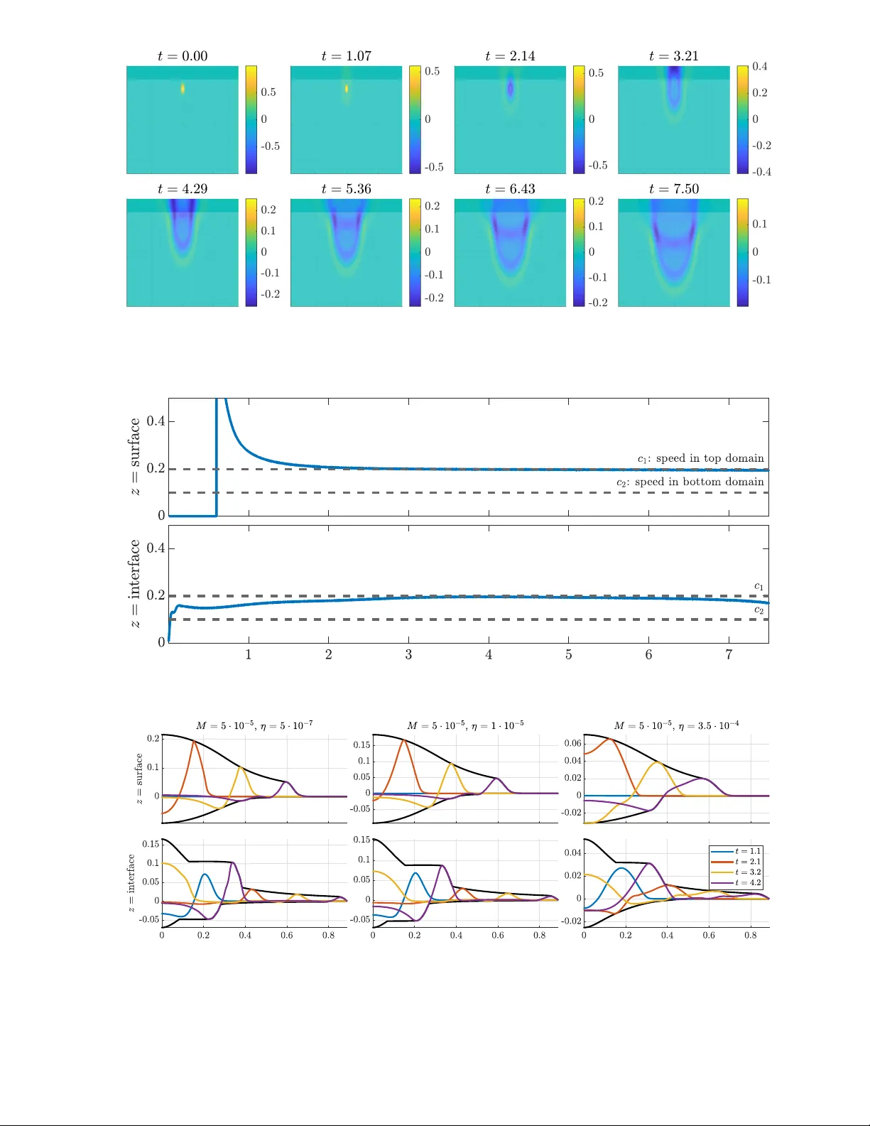
Nonlinear Incompressible Shear W a v e Mo dels in Hyp erelasticit y and Visco elasticit y F ramew orks, with Applications to Lo v e W av es Sha wn Sam uel Carl McAdam ∗ 1 , Sam uel Opoku Agyemang † 1 , and Alexei Cheviak ov ‡ 1 1 Departmen t of Mathematics and Statistics, Universit y of Sask atc hew an Marc h 20, 2026 Abstract General equations describing shear displacemen ts in incompressible h yp erelastic mate- rials, holding for an arbitrary form of strain energy densit y function, are presented and applied to the description of nonlinear Lov e-type w av es propagating on an in terface b e- t ween materials with diﬀeren t mec hanical properties. The mo del is v alid for a broad class of h yp er-visco elastic materials. F or a cubic Y eoh mo del, shear w av e equations contain cubic and quintic diﬀerential p olynomial terms, including viscoelasticity con tributions in terms of dispersion terms that include mixed deriv ativ es u xxt of the material displacement. F ull (2+1)-dimensional n umerical sim ulations of wa ves propagating in the bulk of a tw o-lay ered solid are undertaken and analyzed with resp ect to the source p osition and mec hanical prop- erties of the lay ers. In terfacial nonlinear Lov e wa ves and free upp er surface shear wa ves are track ed; it is demonstrated that in the fully nonlinear case, the v ariable w av e sp eed of interface and surface wa ves generally satisﬁes the linear Lov e w av e existence condition c 1 < | v | < c 2 , while tending to the larger material wa ve sp eed c 1 or c 2 for large times. 1 In tro duction The study of nonlinear shear w av es propagating through an elastic material is fundamentally imp ortan t in v arious areas of science and tec hnology , including material sciences, seismology , geology , natural resource exploration, biological material researc h, and further medical appli- cations. T o brieﬂy review, an elastic material resists external forces and returns to its original form when suc h forces are remov ed (unless the forces are too extreme, causing the material to yield and deform plastically). Commonly , models of elastic materials assume Ho oke’s law, where stress is linearly related to strain. This assumption holds for most materials undergoing small deformations, but neglects nonlinear eﬀects in the stress-strain relation. The present w ork considers ﬁnite deformations of h yp erelastic materials that p ossess a scalar strain energy densit y function W H determining the stress-strain relationship (Section 3 ). Materials such as polymers, rubb ers, foams, and biological tissues exhibit essen tial nonlinear elastic behaviour when they undergo large elastic deformations. This nonlinear elastic behaviour under load or prescribed displacemen t can be modeled through a phenomenological approac h [ 1 ], ph ysical description approach [ 2 ], or use of exp erimen tal data [ 3 ]. The strain energy densit y is ∗ Electronic mail: ssm259@usask.ca † Electronic mail: soa964@usask.ca ‡ Corresp onding Author. Alternative English sp elling: Alexey Shevy ako v. Electronic mail: alexei.che viako v@usask.ca 1 commonly either p ostulated from theoretical considerations or ﬁtted in a certain form from exp erimen tal measurements. The form of the strain energy density is stated in terms of the deformation in v ariants such as principal stretches or matrix in v ariants of Cauch y-Green defor- mation tensors. In addition to h yp erelastic behaviour, one ma y include viscoelastic constitutiv e mo del contributions through, for example, a pseudo-strain energy densit y function dep ending on the rate of c hange of a deformation tensor [ 4 ]. A ma jor application area of linear elasticity theory is seismology . The fundamen tals of seismic w av e theory are built upon the seismic w av e equation modelling a displacement u ( x 1 , x 2 , x 3 ) = ( u 1 , u 2 , u 3 ) propagating through a linear, roughly isotropic material, suc h as Earth lay ers and geological formations: ρ ∂ 2 u i ∂ t 2 = ( λ + µ ) ∂ ∂ x i div u + µ ∆ u i , (1.1) where the Lam ´ e parameters λ, µ > 0 and the densit y ρ > 0 may b e assumed piecewise constant [ 5 ]. The seismic w av e equation follo ws from the equations of motion of a contin uum b o dy and Ho ok e’s law for isotropic materials. T aking λ, µ, and ρ to be piecewise constan t allows one to mo del some of Earth’s anisotrop y , typically as a stack of isotropic lay ers. The full seismic wa v e equation takes the Lam ´ e parameters to b e piecewise smo oth functions of ( x 1 , x 2 , x 3 ), adding complexit y to the equation. Using equation ( 1.1 ), one can determine that the div ergence and curl of u are describ ed b y D’Alem b ert’s equation (the linear wa v e equation) with wa ve sp eeds p ( λ + 2 µ ) /ρ and p µ/ρ resp ectiv ely . Compressional P–w a ves are solutions to the PDE for div u and transverse S–wa v es are solutions to the PDE for curl u . In particular, P–wa v es trav el faster than S–wa ves. P– and S–wa v es are bo dy w av es, and their energy deca ys as 1 /r 2 , where r is the distance from the wa v e front to the fo cus of the initial displacement that caused them, suc h as an earthquake. Surface wa v es tra vel along the surface of the Earth at a slo w er rate than b ody w a ves, but preserv e more of their energy , deca ying as 1 /r . As such, surface w av es dominate seismograms at large distances from an earthquak e’s fo cus and cause a ma jorit y of the damage to h uman structures. One type of surface wa v e is the Lov e wa ve. Lo ve wa v es are horizon tally p olarized transv erse w av es, referred to as shear or SH-wa ves. Ov er large spatial scales (to o large for the ﬂat Earth approximation to apply), Lo v e wa v es form from the interference of S–w av es rep eatedly reﬂecting oﬀ the slowly curving surface of the Earth [ 5 ]. A simpliﬁed model of Lov e wa v es considers t wo isotropic, homogeneous materials in the plane R 2 , that is, the ﬂat-Earth model. The ﬁrst material is represented b y a horizon tal strip of thic kness L , and o verla ys the second material, occupying the space b elo w a horizontal line, say z = 0. W e refer to the line z = 0 as the interface, and the line z = L as the surface. When the materials p ossess diﬀering Y oung’s mo duli, displacements betw een them trav el at diﬀering rates c 1 and c 2 resp ectiv ely . Lo ve wa ves are taken to b e the wa ves that result from the in teractions along the interface of the t wo media. Section 2 reviews this mo del in more detail, and includes an illustration of the domain (Figure 2.1 ). In the fully linear case, it is kno wn that Lo ve wa v es only exist when c 1 < c 2 , whic h we call the Lov e w av e existence condition. The phase velocity v of a Lov e wa ve satisﬁes c 1 < | v | < c 2 . (1.2) Consequen tly , for shear wa v es propagating through linear elastic materials, the discon tin uous w av e sp eed determines the range of allo wable phase velocities. If a seismic ra y attempts to cross the in terface but its angle of incidence is to o large, then the ray is completely reﬂected (b y Snell’s la w). Such seismic rays are then trapped in the upp er lay er in perp etuit y , making the upp er la yer a w av e guide for se ismic ra ys with large angles of incidence. If c 2 < c 1 , suc h a reﬂection is imp ossible so ev ery seismic ray even tually decays into the half space. 2 After assuming the appropriate conditions to use the ﬂat Earth approximation (i.e. consider- ing a rectangle with one face on the Earth’s surface and tens of kilometers deep), we may apply the ab ov e Lov e wa v e mo del with the continen tal crust as the upp er lay er, the solid upp ermost man tle as the half-space, and the Mohoro vi ˇ ci ´ c (Moho) discontin uit y as their interface. Below the o ceanic ﬂo or, the Moho is consistently ab out 10 km deep. Belo w con tinental land mass, the Moho can range b et ween 20 km and 70 km in depth, but a verages ab out 40 km deep. W e may consider the Moho to b e of constant depth whenever the ﬂat Earth appro ximation applies. In the present work, we use contin uum mechanics to derive an equation mo delling nonlinear SH w av es, that is, w av es of ﬁnite amplitude, propagating through a hyperelastic, isotropic, incompressible, homogeneous, neo-Ho ok ean material. The mo del generally allows for signiﬁcant freedom through the c hoice of the constitutiv e strain energy density function W H to approximate nonlinear stress-strain curv es. W e sp ecialize the mo del to a particular strain energy densit y similar to those suggested in Murnaghan [ 6 ] and Bland [ 7 ]. The resulting mo del only requires a go od approximation of the neo-Ho okean material’s stress-strain curve with a cubic diﬀerential p olynomial. F urther, the mo del is a consequence of three necessary balance laws in a contin uum b ody: conserv ation of mass and angular momen tum, and the balance of linear mome n tum. The resulting mo del is given by the linear w av e equation with cubic and quin tic p erturbations, and reduces to the linear model of SH w av es for inﬁnitesimal displacements. F urther, our mo del includes the eﬀects of energy dissipation through the use of a viscosit y p oten tial. It is imp ortan t to note that in mo delling m ultiple shear w av e settings, including earthquakes in particular, it is essen tial to consider ﬁnite displacemen ts and resulting nonlinear PDEs. As v eriﬁed in Bataille and Lund [ 8 ] the displacements and strains in earthquakes are small: the t ypical displacements caused by an earthquake ranges from 10 − 10 m to 10 − 1 m and typical earth- quak e strain of the ground ranges from 10 − 6 to 10 − 2 ; how ev er, Bataille and Lund also argued that nonlinear eﬀects should b e included when modelling surface wa ves b ecause suc h nonlin- earities ma y balance out the disp ersion eﬀects in curren t linear Lov e w a ve mo dels. F urther, the displacements due to seismic wa ves are large near the focus of an earthquake. Because the ﬂat Earth appro ximation is only v alid ov er small spatial scales (hence, near the fo cus of the earthquak e), our nonlinear mo del of SH w av es is ideal for the ﬂat Earth mo del of Lov e w av es. Other applications include the description of shear wa v es in biological tissues and other complex materials (see, e.g., [ 9 ]). The remainder of this pap er is organized as follo ws. In Section 2 , w e review the Linear theory of Lo ve wa v es and the corresp onding solutions. In Section 3 , w e review the equations of motion and constitutiv e mo dels of fully nonlinear h yp erelastic b o dies in the material (Lagrangian) framew ork. In Section 4 , we derive a general partial diﬀerential equation mo del describing the propagation of one- and t w o-dimensional shear wa v es in incompressible hyperelastic materials for an arbitrary strain energy density function. In Section 5 , we generalize the work in Section 4 to include visco elastic eﬀects. In particular, we derive the hyper-visco elastic equation of motion satisﬁed by shear w av es in the cubic Y eoh model framework. In Section 6 , w e numerically analyze the qualitative b eha viour of solutions to the Lo ve w av e equation with ﬁnite displacemen ts. In particular, w av e fronts are eﬃciently track ed, and it is shown that, similar to the linear framew ork, the nonlinear Lo ve-t yp e wa v e speeds generally satisfy the inequality ( 1.2 ). In Section 7 , we use symmetry methods to deriv e exact scaling-in v ariant solutions to our mo del in one spatial dimension. Though unbounded, with certain mo diﬁcations, these solutions provide close agreemen t to the observed n umerical b eha viour. 3 2 Linear theory of Lo v e wa v es In tw o-dimensional space, consider an isotropic la yer of heigh t L o verlying an isotropic elastic half-space and lab el their in terface with the line z = 0. Let u = u ( x, z , t ) be a displacement p erpendicular to this space at the p oin t ( x, z ) and time t . Suppose the displacement u propagates through the space according to the following v ariation of the linear wa v e equation u tt = c ( z ) 2 ( u xx + u z z ) , c ( z ) = ( c 1 if 0 ≤ z < L, c 2 if z < 0 . (2.1) where subscripts denote partial diﬀerentiation whenev er appropriate. W e refer to equation ( 2.1 ) with piecewise constan t wa v e speed as the linear Lo v e w a ve equation. This equation mo dels materials whose elemen ts hav e a linear restoring force resulting from Hooke’s la w. The wa ve sp eed c 2 is tak en to b e a piecewise-constan t function of z b ecause the speed of propagation dep ends on v arious prop erties of the t w o media. Lov e w av es will propagate b et w een the in terface and the upp er b oundary z = L (which we refer to as the surface of this domain). The surface is stress-free, corresp onding to a Neumann b oundary condition u z ( x, L, t ) = 0. A t z → −∞ , u → 0 is assumed. Figure 2.1 illustrates this mo del. + x − z u ( x, −∞ , t ) = 0 F ree space Medium 1: u tt = c 2 1 ( u xx + u z z ) Medium 2: u tt = c 2 2 ( u xx + u z z ) Surface z = L In terface z = 0 ∂ u/∂ z | z = L = 0 Figure 2.1: An isotropic la yer ov erlying an isotropic elastic half-space. The y direction is p erpendicular to this space spanned by x, z . The p ositiv e z direction p oin ts down wards, L is the depth of the isotropic lay er, wa ves tra velling through the isotropic lay er (medium 1) hav e sp eed c 2 1 , and wa ves tra velling through the isotropic elastic half-space (medium 2) hav e sp eed c 2 2 . Commonly , one solves this problem by assuming that for ﬁxed z , a Lo ve w av e has the form of a plane wa v e trav elling along the x direction [ 10 ], u ( x, z , t ) = f ( z ) e ik ( x − v t ) , (2.2) where k is the w av e num b er, v is the phase v elo cit y of the wa v e, and f is some contin uously diﬀeren tiable function of the depth z . Here we aim to solv e for f and ﬁnd an expression for k as a function of v . Note that for ( 2.2 ) to represen t a Lov e w av e, f must decay exp onen tially as z → −∞ . F urther, observ e that the phase v elo cit y is assumed to not dep end on depth z . Substituting ( 2.2 ) into the piecewise linear wa ve equation implies f ′′ ( z ) = k 2 (1 − ( v /c ( z )) 2 ) f ( z ) = ( k 2 (1 − ( v /c 1 ) 2 ) f ( z ) if 0 ≤ z < L, k 2 (1 − ( v /c 2 ) 2 ) f ( z ) if z < 0 , (2.3) 4 and the b oundary conditions imply f ′ ( L ) = f ( −∞ ) = 0. F or any ﬁxed v alue of v , equation ( 2.3 ) b ecomes a Sturm–Liouville b oundary v alue problem (BVP) ( p ( z ) f ′ ( z )) ′ + q ( z ) f ( z ) = − λr ( z ) f ( z ) , where p = 1 , q = 0 , λ = k 2 , and r ( z ) = 1 − ( v /c ( z )) 2 . Recall that for an Sturm–Liouville BVP to b e r e gular , the w eight function r ( z ) m ust b e a p ositive, contin uous function ov er its domain. The ODE in equation ( 2.3 ) is irr e gular b ecause r ( z ) is discontin uous at 0. F or ev ery | v | ∈ ( c 1 , c 2 ) and every n ∈ Z , the following is a coun table set of eigenv alue/function pairs ( k n ( v ) , f n ( z ; v )) for the ab o ve Sturm–Liouville BVP: f n ( z ; v ) = ( cos( k n ( v )Ω 1 ( v )( z − L )) 0 ≤ z < L, cos( k n ( v )Ω 1 ( v ) L ) e | k n ( v ) | Ω 2 ( v ) z z < 0 , (2.4) where Ω 1 ( v ) = p ( v /c 1 ) 2 − 1 , Ω 2 ( v ) = p 1 − ( v /c 2 ) 2 . The deriv ative f ′ n ( z ; v ) must b e contin uous at L , so Ω 1 ( v ) and Ω 2 ( v ) are related by Ω 2 ( v ) = sign( k n ( v ))Ω 1 ( v ) tan( k n ( v )Ω 1 ( v ) L ) . (2.5) Both functions Ω 1 ( v ) , Ω 2 ( v ) must output nonnegativ e real num b ers for the solution f n to satisfy the b oundary conditions and b e contin uously diﬀeren tiable at the in terface z = 0. This deter- mines the range of allow able phase v elo cities v , also called the L ove wave existenc e c ondition ( 1.2 ): c 1 < | v | < c 2 . (2.6) The Lo ve w av e existence condition also implies the w eight function r ( z ) ≤ 0 for z ∈ [0 , L ), which is another reason why the Sturm–Liouville BVP ( 2.3 ) is not regular. One can use equation ( 2.5 ) to solve for eac h eigenv alue k n ( v ), k n ( v ) = 1 L Ω 1 ( v ) (sign( n ) arctan(Ω 2 ( v ) / Ω 1 ( v )) + πn ) = c 1 L p v 2 − c 2 1 sign( n ) arctan c 1 c 2 s c 2 2 − v 2 v 2 − c 2 1 ! + π n ! = sign( n ) k 0 ( v ) + π n L Ω 1 ( v ) . Because k 0 ( v ) is nonzero, there are tw o distinct eigenv alues ± k 0 ( v ) corresp onding to 0, whic h w e lab el with ± k 0 ( v ) = k ± 0 ( v ). W e observe that k − n ( v ) = − k n ( v ) for every n (including n = 0) so the eigenfunctions satisfy f − n ( z , v ) = f n ( z , v ). Eac h eigenfunction then corresponds to t w o distinct eigenv alues ± k n ( v ). The negative n eigenfunctions do not yield new linearly independent solutions; how ever, the ov erall solution mo de f n ( z , v ) e ik n ( v )( x − vt ) do es c hange. Now that w e ha ve an equation for k n , we see that the inequalities are strict in ( 1.2 ) because f n ( z , c 2 ) = ( − 1) n for z < 0 (hence do es not decay as z → −∞ ) and f n ( z , c 1 ) is not contin uously diﬀeren tiable at z = 0. Indeed, f n ( z , c 1 ) = 0 for z ≤ 0 (b ecause k n has a p ole at c 1 ) and ∂ z f n ( z , c 1 ) | z =0 + = − k n ( c 1 )Ω 1 ( c 1 ) sin( k n ( c 1 )Ω 1 ( c 1 ) L )  = 0. There is a countably inﬁnite set of w av e n umbers k n ( v ) corresp onding to a giv en phase velocity v . W e note that k n ( v ) , Ω 1 ( v ) , Ω 2 ( v ) , and f n ( z ; v ) are all even with resp ect to v , so we need only study these function for p ositiv e v . Each k n ( v ) is a strictly decreasing function of v ∈ ( c 1 , c 2 ) 5 for n ≥ 0 b ecause Ω 1 ( v ) strictly increases, Ω 2 ( v ) / Ω 1 ( v ) strictly decreases, and arctan strictly increases. As such, k n ( v ) realizes its minimum at v = c 2 and we hav e the follo wing low er b ound on each k n ( v ), k n ( v ) ≥ k 0 ( c 2 ) + π n L Ω 1 ( c 2 ) ≥ n π c 1 L p c 2 2 − c 2 1 . This result implies there are ﬁnitely man y phase velocities v corresponding to a giv en wa v e n umber k ∗ . F urther, k n restricted to [ c 1 , c 2 ] is in vertible and its in verse has the domain [ nπ c 1 . L p c 2 2 − c 2 1 , sign( n ) ∞ ]. Figure 2.2 plots f n ( z ; v ′ ) for x ∈ [0 , 3 L ] with v ′ = ( c 1 + c 2 ) / 2, and k n ( v ) for v ∈ [ c 1 , c 2 ] b oth for v arious v alues of n . Increasing n by 1 increases k n ( v ) by π / ( L Ω 1 ( v )). This has the eﬀect of increasing the frequency of oscillations of f n ( z ; v ) for z ∈ [0 , L ], and mak es f n ( z ; v ) decay faster for z ≥ L . Increasing n also mak es u ( x, z , t ) = f n ( z ; v ) e ik n ( v )( x − vt ) oscillate more along the x direction. This is illustrated in Figure 2.3 whic h contains plots of fundamental solutions to equation ( 2.1 ) for v arious n and v . Figure 2.2: Left: plots of f 0 ( z ; v ), f 1 ( z ; v ), f 2 ( z ; v ), and f 3 ( z ; v ) for z ∈ [0 , 3 L ] and v = ( c 1 + c 2 ) / 2. Right: plot of k n ( v ) o ver v ∈ [ c 1 , c 2 ] for n = 0 , 1 , 2 , 3. Recall that k n ( v ) strictly increases with n . Other parameters are L = 1, c 1 = 1, c 2 = 2 Figure 2.3: The real part of fundamental solutions f n ( z ; v ) e ik n ( v )( x − v t ) to equation ( 2.1 ) for v arious v and n , with c 1 = 1, c 2 = 2, and L = 1. A solution of the form f n ( z ; v ) e ik n ( v )( x − vt ) exists for each | v | ∈ ( c 1 , c 2 ) and each n ∈ Z . Let D = ( − c 2 , − c 1 ) ∪ ( c 1 , c 2 ), then the most general plane wa v e solution to the linear Lov e w av e 6 equation ( 2.1 ) is of the form u ( x, z , t ) = ∞ X n = −∞ Z D α n ( v ) f n ( z ; v ) e ik n ( v )( x − vt ) d v (2.7) where w e recall that the solution corresponding to n = 0 is coun ted t wice in the ﬁrst line because there are tw o distinct 0 th mo des with eigenv alues ± k 0 ( v ). W e determine the co eﬃcien ts α n ( v ) from suﬃcien tly smo oth initial conditions u ( x, z , 0) = F ( x, z ) and u t ( x, z , 0) = G ( x, z ). Because f n and k n are even ov er v , we hav e F ( x, z ) = ∞ X n = −∞ Z c 2 c 1 ( α n ( v ) + α n ( − v )) f n ( z ; v ) e ik n ( v ) x d v . (2.8) W e can write this as an in verse F ourier transform b y substituting w = k n ( v ). W e observe that the b ounds on eac h integral no w depend on n as shown in the following. Let b n = | n | π c 1 . L p c 2 2 − c 2 1 , then F ( x, z ) = − ∞ X n =0 Z ∞ b n [ α n ( k − 1 n ( w )) + α n ( − k − 1 n ( w ))] k ′ n ( k − 1 n ( w )) f n ( z ; k − 1 n ( w )) e iwx d w + ∞ X n =0 Z − b n −∞ [ α − n ( k − 1 − n ( w )) + α − n ( − k − 1 − n ( w ))] k ′ − n ( k − 1 − n ( w )) f n ( z ; k − 1 − n ( w )) e iwx d w . W e can signiﬁcantly simplify this in tegral b y deﬁning the sequence A 0 , A 1 , . . . of piecewise functions, A n ( w ) =      α n ( k − 1 n ( w )) + α n ( − k − 1 n ( w )) if w ≥ b n , α − n ( k − 1 − n ( w )) + α − n ( − k − 1 − n ( w )) if w ≤ − b n , 0 otherwise. F urther, k − n ( v ) = − k n ( v ), so we hav e k − 1 − n ( w ) = k − 1 n ( − w ). In total, F ( x, z ) = − Z ∞ −∞ e iwx ∞ X n =0 A n ( w ) k ′ n ( k − 1 n ( | w | )) f n ( z ; k − 1 n ( | w | )) d w , and applying the inv erse F ourier transform to b oth sides results in 1 2 π Z ∞ −∞ F ( x, z ) e − iwx d x = − ∞ X n =0 A n ( w ) k ′ n ( k − 1 n ( | w | )) f n ( z ; k − 1 n ( | w | )) . The eigenfunctions from ( 2.3 ) are orthogonal with resp ect to the weigh t function r ( z ; v ) = 1 − ( v /c ( z )) 2 . They satisfy the equation Z L −∞ f n ( z ; v ) f m ( z ; v ) r ( z ; v )d z = ( − L 2 Ω 1 ( v ) 2 if | m | = | n | , 0 otherwise, where the minus sign app ears in the r − norm because r ( z ; v ) < 0 for 0 ≤ z < L . With this, we isolate for each term in the summation ab o ve b y m ultiplying each side by f n ( z ; k − 1 n ( | w | )) r ( z , k − 1 n ( | w | )) and integrating o ver z . The resulting form ula for each A n ( w ) is, A n ( w ) = k ′ n ( k − 1 n ( | w | )) π L Ω 1 ( k − 1 n ( | w | )) 2 Z L −∞ Z ∞ −∞ F ( x, z ) f n ( z ; k − 1 n ( | w | )) r ( z ; k − 1 n ( | w | )) e − iwx d x d z 7 With this, we are halfwa y to solving for each α n ( v ) b ecause, A n ( ± k n ( v )) = k ′ n ( v ) π L Ω 1 ( v ) 2 Z L −∞ Z ∞ −∞ F ( x, z ) f n ( z ; v ) r ( z ; v ) e ∓ ik n ( v ) x d x d z = α ± n ( v ) + α ± n ( − v ) , n ≥ 0 . With the initial condition for u t ( x, z , 0) = G ( x, z ) and the same logic as presen ted ab o v e, we compute a similar formula for the diﬀerence b et ween tw o co eﬃcien ts, ± ( α ± n ( v ) − α ± n ( − v )) = ik ′ n ( v ) π L Ω 1 ( v ) 2 v k n ( v ) Z L −∞ Z ∞ −∞ G ( x, z ) f n ( z ; v ) r ( z ; v ) e ∓ ik n ( v ) x d x d z . F or our purposes, w e only consider u t ( x, z , 0) = 0, so α n ( v ) = α n ( − v ), α − n ( v ) = α n ( v ), and the solution takes the form u ( x, z , t ) = 4 ∞ X n =0 Z c 2 c 1 f n ( z ; v ) cos( k n ( v ) v t ) Re  α n ( v ) e ik n ( v ) x  d v . Implicit in the assumption ( 2.2 ) is that the phase does not c hange with depth z . This assumption is carried through to Equation ( 2.7 ). As a consequence of this assumption and the fact that the Sturm-Liouville problem ( 2.3 ) is not regular, the set of eigenfunctions { f n } is not complete. The decomp osition ( 2.8 ) holds only for a subset of initial conditions of the problem for ( 2.1 ). In Section 6.2 , w e use the metho d of lines to numerically study the initial b ehaviour of linear and nonlinear Lov e wa v es sub ject to a sudden explosion. While doing so, we record the velocity of the wa v es trav elling horizontally along the surface and interface. W e ﬁnd that these velocities initially diﬀer, but even tually take on the same v alue. As suc h, the solution w e derived can describ e suﬃciently large-time b eha viour of a Lov e w av e moving along the x direction. 3 Nonlinear h yp erelasticit y and constitutiv e mo dels The h yp erelasticit y framework provides a natural generalization of linear w av es corresp onding to small displacements in nonlinear materials, including geological formations, to the case where displacemen ts are not small. In this section, we describ e the b eha viour of incompressible hyper- elastic media undergoing ﬁnite (p ossibly large) strains when sub jected to external stress. W e brieﬂy recall the notation and the main ingredien ts of mathematical models in incompressible h yp erelasticit y required for this study (see, e.g., Refs. [ 11 – 14 ] for full details). V ectors and ten- sors are indicated with boldface characters and their en tries are written in italics. En tries of v ectors and tensors are written in italics, and summation in rep eated indices is assumed where appropriate. W e use Cartesian co ordinates and the ﬂat space metric g ij = δ ij . 3.1 Hyp erelastic materials: equations of motion Consider an elastic solid parameterized by material (Lagrangian) co ordinates X = ( X , Y , Z ) = ( X 1 , X 2 , X 3 ) in a spatial region Ω 0 ⊂ R 3 with a piecewise-smo oth boundary . W e call Ω 0 the reference conﬁguration or the natural state of the solid. After deformations, the actual shap e of the solid at time t is given by the time-dependent Eulerian co ordinates x = ( x, y , z ) = ( x 1 , x 2 , x 3 ) in the actual conﬁguration Ω ⊂ R 3 . The Eulerian co ordinates can be in terpreted as an in vertible, smo oth, orientation-preserving map deforming the b o dy ov er time, x = x ( X , t ) = X + u ( X , t ) . (3.1) 8 The map x is also referred to as a deformation ﬁeld. u = u ( X , t ) has the meaning of displacement and is not assumed to b e small. Figure 3.1 illustrates this situation along with area elements, the normal vector N ab out a p oin t X in the reference conﬁguration, and its corresp onding normal v ector n p oin t x in the actual conﬁguration. The velocity and the acceleration of a material p oin t X are given by v ( X , t ) = ∂ x / ∂ t and a ( X , t ) = ∂ 2 x  ∂ t 2 . W e aim to describ e a system of PDEs describing the deformation ﬁeld x in terms of its deriv atives in X and t . The deformation gradient F is the Jacobian of x with resp ect to X , F ( X , t ) = grad X x , F i j = ∂ x i ∂ X j . (3.2) Because x is an orientation-preserving map, J ≡ det( F ) > 0. The map x preserv es volumes for incompressible materials, so J = 1. W e note that when reasonable, w e write formulae in terms of general J , and then substitute J = 1. If the densit y of the elastic material in the Lagrange conﬁguration is represented by ρ 0 = ρ 0 ( X ), the current time-dep enden t mass density in Lagrangian co ordinates tak es the form ρ ( X , t ) = ρ 0 ( X ) /J = ρ 0 ( X ) . The left and righ t Cauc hy-Green deformation tensors B = FF T and C = F T F play an essen tial role in the form ulation of the equations of motion in solid mec hanics. F or our purp oses, w e regard B and C as matrices to av oid unnecessary tensor algebra. B and C are symmetric p ositiv e-deﬁnite and share the same set of eigenv alues. The square ro ots of these eigenv alues determine the singular v alues ( σ 1 , σ 2 , σ 3 ) of F which are referred to as the principal stretches. Let t b e the traction v ector representing force p er unit area acting on the area element d a with unit normal vector n in the actual conﬁguration. According to the Cauch y theorem, t = σ n , where σ = σ ( x , t ) is the symmetric Cauch y stress tensor. Let T b e the corresp onding traction vector in the reference conﬁguration acting on the undeformed area element d A with unit normal vector N . T is giv en by T = PN , where P = P ( X , t ) denotes the asymmetric ﬁrst Piola-Kirc hhoﬀ stress tensor, related to the Cauc h y stress through P = J σ F − T . Here F − T is the in verse of the transp ose of F . The equations of motion of x are given directly in terms of P . The second Piola-Kirchhoﬀ stress tensor S is given in terms of the deformation gradient F and the ﬁrst Piola-Kirchhoﬀ stress tensor P by S = F − 1 P . Figure 3.1: A general illustration of the deformation x ( X , t ) acting on the reference conﬁguration after some time t . The stress tensors P and S can b e explicitly determined b y assuming the form of x (e.g. through sp eciﬁcation of v ariables X 1 , X 2 , or X 3 or their com binations that x 1 , x 2 , or x 3 de- p end on) and a scalar-v alued volumetric h yp erelastic strain energy densit y W H = W H ( X , F ) 9 (sometimes called stored energy density function). In the incompressible hyperelasticity frame- w ork, the Piola-Kirchhoﬀ stress tensors are determined by the strain energy density through the form ulas P = − p F − T + ρ 0 ∂ W H ∂ F = FS , S = − p C − 1 + 2 ρ 0 ∂ W H ∂ C , (3.3) where p = p ( X , t ) denotes h ydrostatic pressure. Partial deriv atives tak en with resp ect to a matrix/tensor are interpreted as a symmetrized partial deriv ative with resp ect to each entry of the matrix/tensor. F or example, the en tries of ∂ W H  ∂ C are given b y  ∂ W H ∂ C  ij = 1 2  ∂ W H ∂ C ij + ∂ W H ∂ C j i  . (3.4) F or isotropic, homogenous, frame-indiﬀeren t, hyperelastic media, the strain energy densit y function can b e written as a function of the three principal in v arian ts I 1 , I 2 , and I 3 of the Cauc hy-Green deformation tensors B and C W H = W H iso ( I 1 , I 2 , I 3 ) . (3.5) The principal inv ariants are the co eﬃcients of the characteristic p olynomial of B , I 1 = tr( B ) , I 2 = 1 2  I 2 1 − tr  B 2  , I 3 = det( B ) = J 2 . (3.6) Generally , a set of inv arian ts can b e an y indep enden t combination of principal stretc hes (meaning they cannot b e written in terms of the other in v ariants). Because x preserves v olumes (i.e. I 3 = J 2 = 1), the strain energy density has a simpler form W H = W H ( I 1 , I 2 ). W e note that when mo delling anisotropic materials, W H additionally dep ends on direction of anisotropy , suc h as the direction of embedded ﬁb ers, through additional inv arian ts (see, e.g., [ 9 , 11 , 12 ] and references therein). The form ulae for W H only in volv e its partial deriv atives, so we may choose the constan t term. Observe that in the natural state x = X , the deformation gradien t F = I is the identit y matrix, and I 1 = I 2 = n in n dimensions. In three dimensions, it is common to tak e W H = W H ( I 1 − 3 , I 2 − 3) . (3.7) W e may then tak e W H (0 , 0) = 0 in the natural state. The follo wing are examples of strain energy density functions. Mo oney-Rivlin solids obey the follo wing strain energy density function W H = a ( I 1 − 3) + b ( I 2 − 3) , (3.8) where a, b ≥ 0 are constant parameters. An y incompressible, lubb er-lik e material is a Mo oney- Rivlin solid. F or b = 0, ( 3.8 ) reduces to the strain energy density function of a neo-Ho ok ean material W H = a ( I 1 − 3) . The linear w a ve equation is the equation of motion for shear wa ves tra v elling through a neo- Ho ok ean solid. There are generalized v ersion of both the Mo oney-Rivlin and neo-Ho ok ean mo dels. The generalized Mo oney-Rivlin function is a biv ariate p olynomial in I 1 − 3 and I 2 − 3, W H = k X i =0 l X j =0 c ij ( I 1 − 3) i ( I 2 − 3) j , (3.9) 10 where c ij are constan t material co eﬃcien ts with c 00 = 0. These model what are called p olynomial-t yp e materials [ 15 ]. One such generalized Mo oney-Rivlin function is the Murnaghan p oten tial. In a t wo-dimensional setting, the Murnaghan p oten tial has b een recently emplo yed in Ref. [ 16 ] to deriv e a w eakly nonlinear analog of the L ove hyp othesis (whic h relates the ra- dial displacement and the longitudinal strain) for a wa v e propagation mo del in an elastic ro d undergoing shear and longitudinal axially symmetric displacements. The generalized neo-Ho ok ean mo del takes the strain energy density function to b e any func- tion of I 1 − 3 without a dep endence on I 2 − 3, W H = W H ( I 1 − 3) . Muc h of the following is restricted to generalized neo-Ho ok ean materials b ecause allowing W H to dep end on I 2 signiﬁcan tly complicates the equations of motion. W e apply the results of the follo wing section to a Y eoh mo del [ 17 ] W H = k X i =0 c i ( I 1 − 3) i , (3.10) with k = 3, resulting in the p olynomial W H = µ ( I 1 − 3) + 1 2 M ( I 1 − 3) 2 + 1 3 A ( I 1 − 3) 3 , (3.11) where µ, M , A are constan ts. F or theoretical reasons explained shortly , it is also desireable for W H to be a con v ex p olynomial. The coeﬃcients of the abov e polynomial mo dels can b e ﬁt to a given material’s stress-strain curv e. F urther generalizations to the ab o v e strain energy densit y functions are p ossible and can b e found in, e.g., [ 18 , 19 ]. These are useful if a material’s stress-strain curve do es not accurately ﬁt to the ab o ve forms. It is desirable for the strain energy density function to b e p olyc onvex . This is the case for generalized Mooney-Rivlin functions (and their sp ecializations) whenev er c ij ≥ 0 for eac h i, j [ 11 ]. Mo dels built from a p olycon vex strain energy density function hav e the following three desirable properties. First, increasing the strain increases the elastic energy . Second, the natural state corresp onds to a stable equilibrium. Lastly , p olyconv exit y guarantees the existence of solutions of b oundary v alue problems in linear elasticity [ 20 ]. Many realistic materials p ossess the ﬁrst t wo prop erties, so they should b e mo delled b y p olycon vex strain energy densit y functions. The last prop erty is desirable in practice. T o provide the mathematical deﬁnition of p olyconv exit y , a real v alued function G = G ( F ) of 3 by 3 tensors is p olycon vex if it can b e written as G ( F ) = g ( F , cof F , det F ) where g is a (t ypically nonunique) conv ex function of the entri es of F , F ’s matrix of cofactors cof F , and det F [ 12 ]. F or the examples, supp ose h : R → R is con v ex. Any function of the form G ( F ) = h (det F ) is polyconv ex but not necessarily con vex with respect to the entries of F . F urther, G ( F ) = h ( | F | ) where | F | denotes the F rob enius norm of F is both p olycon v ex and con vex with resp ect to the entries of F . The full system of equations of motion for incompressible hyperelastic materials in three dimensions is given by ρ 0 ∂ 2 x ∂ t 2 = div X P + D f , (3.12a) PF T = FP T , (3.12b) J = det( F ) = 1 , (3.12c) 11 where D f are the b o dy forces p er unit volume (e.g. gra vity). The i th comp onen t of the divergence of the tensor P with resp ect to the Lagrangian co ordinates X is the div ergence of the i th ro w of P . So, (div X P ) i = div X  P i  = ∂ ∂ X j P i j . The equations of motion are a result of three practical balance la ws (conserv ation of mass and angular momen tum, and balance of linear momentum). The balance law ( 3.12a ) is known as the momentum equation. Equation ( 3.12a ) expresses a conserv ation law if D f = 0, where it b ecomes a total div ergence. The condition ( 3.12b ) expresses conserv ation of angular momentum and is equiv alen t to requiring the Cauc hy stress tensor b e symmetric σ = σ T . F or isotropic materials, as well as in some other cases, this symmetry condition is iden tically satisﬁed (e.g., Ref. [ 19 ]). T o summarize (and provide a preview of the following), one can use equation 3.12 to mo del an incompressible hyperelastic material after assuming the form of x , ﬁtting a strain energy densit y function W H to their material’s stress-strain curv e, and then ﬁnding the ﬁrst Piola- Kirc hhoﬀ stress tensor. This pro cess is made easier when the material is isotropic, homogenous and frame-indiﬀeren t because then W H is a function of three arguments (the principal in v ariants of B = FF T ). In that case , one can assume a general form for W H , then the PDE ( 3.12a ) will mo del any material whose stress- strain curv e is well approximated b y such W H . 4 Nonlinear h yp erelastic shear w a v es 4.1 The general wa ve equation for an arbitrary strain energy densit y function Consider a shear wa ve with displacements in the Y − direction propagating through the X − Z plane (which is antiplane motion) describ ed by x =   x y z   =   X Y Z   +   0 v ( t, X , Z ) 0   . (4.1) Our aim is to deriv e the equations of motion for v ( X , Z , t ). As discussed in Sec tion 3 , these follo w from computing P . The deformation gradien t and its inv erse are F =   1 0 0 v X 1 v Z 0 0 1   , F − 1 =   1 0 0 − v X 1 − v Z 0 0 1   , (4.2) where v X = ∂ v / ∂ X , and v Z = ∂ v / ∂ Z represen t the amoun t of shear. The left and righ t Cauc hy-Green deformation tensors B and C are C =   1 + v 2 X v X v X v Z v X 1 v Z v X v Z v Z 1 + v 2 Z   , B =   1 v X 0 v X v 2 X + v 2 Z + 1 v Z 0 v Z 1   . (4.3) The principal inv ariants for the deformation ﬁeld ( 4.1 ) are I 1 = I 2 = 3 + v 2 X + v 2 Z = 3 + ∥ grad v ∥ 2 = | F | 2 , I 3 = 1 . where | F | is the F rob enius norm of F . The shear displacemen ts ( 4.1 ) are naturally incompressible b ecause I 3 = det( F ) = 1. It is imp ortan t to note that, although I 1 = I 2 , w e cannot use this 12 fact until after expanding ( 3.3 ) and ( 3.4 ). Doing otherwise would miss a necessary condition to ensure the pressure is well deﬁned. Equation ( 3.3 ) yields the ﬁrst Piola-Kirchhoﬀ stress tensor P = − p F − T + 2 W H 1 F − 2 W H 2 B − 1 F − T , (4.4) where W H = W H ( I 1 , I 2 ), W H 1 ≡ ∂ W H ∂ I 1 , W H 2 ≡ ∂ W H ∂ I 2 , and p = p ( X , Z , t ). Substituting ( 4.4 ) in to the equations of motion ( 3.12a ) yield the following system of PDEs q X + 2( W H 2 v 2 X ) X + 2( W H 2 v X v Z ) Z = 0 , q Z + 2( W H 2 v X v Z ) X + 2( W H 2 v 2 Z ) Z = 0 , (4.5a) ρ 0 v tt = 2  ( v X ( W H 1 + W H 2 )) X + ( v Z ( W H 1 + W H 2 )) Z  , (4.5b) where q = p − 2 W H 1 − 2( v 2 X + u 2 Z + 2) W H 2 . Cross diﬀeren tiating the tw o equations for q in ( 4.5a ) yields the compatibility condition  ( W H 2 v X v Z ) X + ( W H 2 v 2 Z ) Z  X −  ( W H 2 v 2 X ) X + ( W H 2 v X v Z ) Z  Z = 0 . (4.6) This condition can b e written in the language of vector calculus as curl  div  W 2 ( || ∇ v || 2 ) ∇ v ⊗ ∇ v  = 0 . The system ( 4.5 ) and ( 4.6 ) is ov erdetermined. Suc h systems do not t ypically hav e solutions, although the problem’s nonlinearit y makes it diﬃcult to determine existence or uniqueness of solutions with conﬁdence. W e also note that, b ecause I 1 = u 2 X + u 2 Z + 3 = I 2 , there are man y diﬀeren t forms of W H resulting in the same equation ( 4.5b ). The strain in a material undergoing a displacement of the form ( 4.1 ) is a univ ariate function of the stress b ecause one can only observe the v alues of W ( I 1 ) = W H ( I 1 , I 1 ) . (4.7) Fitting W to this material’s stress-strain curv e pro vides no information on W H 1 or W H 2 indi- vidually , but en tirely determines the equation ( 4.5b ) as W ′ ( I 1 ) = W H 1 ( I 1 , I 1 ) + W H 2 ( I 1 , I 1 ). W e a void the intricacies of ( 4.6 ) by restricting our atten tion to generalized neo-Ho ok ean materials, where W H 2 = 0. This restricts the resulting mo del’s applicability in practice, b ecause there are materials that necessarily dep end on I 2 . The issue of determining other conditions on W H suc h that W H 2  = 0 and the compatibilit y condition ( 4.6 ) holds for all solutions to ( 4.5b ) has been explored in [ 21 ]. This issue is outside the scop e of the current w ork. Restricting our attention to generalized neo-Ho ok ean materials also mak es it easier to deter- mine whether a strain energy densit y function is p olycon v ex. In [ 22 , Sec. 2.2], Suc ho c ki et al. state that suc h W H ( I 1 ) is polyconv ex if and only if W H ( I 1 ) is con v ex. As such, w e need only enforce W ′′ > 0. F or generalized neo-Ho ok ean materials (i.e. W H 2 = 0), the equations for the hydrostatic pressure reduce to, p X = 2( W ′ ( v 2 X + v 2 Z )) X , p Z = 2( W ′ ( v 2 X + v 2 Z )) Z , yielding the solution in terms of v X and v Z p = 2 W ′ ( v 2 X + v 2 Z ) + p 0 ( t ) , (4.8) where p 0 ( t ) is the am bient hydrostatic pressure. If the gra vity force e = ρ 0 g e Z is tak en into accoun t, equation ( 4.8 ) is replaced by p = 2 W ′ ( v 2 X + v 2 Z ) + p 0 ( t ) + ρ 0 g Z , with Z directed do wnw ard. 13 Principal Result 1. The Y − displac ement v of a she ar wave given in e quation ( 4.1 ) tr avel ling thr ough a gener alize d ne o-Ho oke an material ( W H 2 = 0 so W = W H ( I 1 ) ) satisﬁes the nonline ar wave e quation ( 4.5b ) , explicitly written as ρ 0 v tt = 2 W ′ ( v 2 X + v 2 Z )( v X X + v Z Z ) + 4 W ′′ ( v 2 X + v 2 Z )( v 2 X v X X + 2 v X v Z v X Z + v 2 Z v Z Z ) . (4.9) W e refer to equation ( 4.5b ), ( 4.9 ) as the gener al nonline ar she ar wave e quation . The PDE ( 4.9 ) is linear if and only if W ′′ ≡ ∂ 2 W H ( I 1 )  ∂ I 2 1 = 0 (i.e. W is linear in its single argument I 1 − 3). This is the case for Mooney-Rivlin materials with strain energy densit y f unction W H = a ( I 1 − 3). In this case, the Y oung’s mo dulus is a , the wa ve equation ( 4.9 ) reduces to the linear PDE ρ 0 v tt = 2 a ( v X X + v Z Z ), and the hydrostatic pressure is p = 2 a + ρ 0 g Z . 4.2 The general nonlinear shear wa ve equation for the cubic Y eoh model Substituting the cubic Y eoh mo del ( 3.11 ) into the general nonlinear shear wa v e equation ( 4.9 ) yields ρ 0 v tt = 2  µ + M  v 2 X + v 2 Z  + A  v 2 X + v 2 Z  2  ( v X X + v Z Z ) +4  M + 2 A ( v 2 X + v 2 Z )  ( v 2 X v X X + 2 v X v Z v X Z + v 2 Z v Z Z ) . (4.10a) The hydrostatic pressure ( 4.8 ) in this case is giv en by p = 2  µ + M ( v 2 X + v 2 Z ) + A ( v 2 X + v 2 Z ) 2  + p 0 ( t ) + ρ 0 g Z. (4.10b) Equations ( 4.10 ) contain nonlinear p olynomial terms of the third and ﬁfth orders in terms of v . Cubic eﬀects are controlled by the co eﬃcien t M and quintic eﬀects by the co eﬃcien t A . W riting equation ( 4.10a ) with gradients ∇ = grad ( X,Z ) mak es it more apparent what eﬀects eac h parameter has and that this equation is a total divergence, ρ 0 2 v tt = div h µ + M ∥ ∇ v ∥ 2 + A ∥ ∇ v ∥ 4 i ∇ v  . (4.11) The expression in square brack ets is W 1 comp osed with ∥ ∇ v ∥ 2 . T o our knowledge, the PDEs ( 4.10 ), ( 4.11 ) hav e not previously app eared in the litera- ture. Similar models of nonlinear shear wa ves based on displacemen ts ( 4.1 ) w ere considered in Kaly anasundaram [ 23 ], T eymur [ 24 ], and Rushc hitsky [ 25 , 26 ], who assumed a compressible h yp erelastic material, and employ ed a diﬀerent (Murnaghan) hyperelastic p oten tial. In our ap- proac h, b ecause the deformation ﬁeld ( 4.1 ) naturally preserves volumes, new nonlinear w a ve equations are coupled to the hydrostatic pressure ﬁelds that dep end on displacemen ts according to ( 4.10b ). W e note that b ecause the nonlinearit y in the PDE ( 4.11 ) inv olv es only gradients, the disp er- sion relation for p erturbations v = v 0 + ϵ exp( i ( k 1 X 1 + k 3 X 3 − ω t )) around a constant equilib- rium v 0 coincides with the linear wa v e equation disp ersion relation ω 2 = 2 µ ρ 0 ( k 2 1 + k 2 3 ) . Ho wev er, if the equation ( 4.11 ) is linearized about a uniform shear solution v = v 0 + sX 1 , s = const, that is, in the ansatz v = v 0 + sX 1 + ϵ exp( i ( k 1 X 1 + k 3 X 3 − ω t )), the dispersion relation takes the form ω 2 = 2 ρ 0  µ ( k 2 1 + k 2 3 ) + M s 2 (3 k 2 1 + k 2 3 ) + As 4 (5 k 2 1 + k 2 3 )  . 14 5 Nonlinear Visco elastic shear w a v es In this section, w e add non-elastic eﬀects resp onsible for ener gy dissip ation to our mo del. Consid- ering b oth elasticit y and viscosit y ensures our mo del of large displacements in nonlinear materials remain realistic o ver long perio ds of time. Materials such as geological formations, comp osite materials, and biological tissues exhibit visco elastic prop erties. V arious approaches exist for the mathematical description of visco elasticit y , including rational and irreversible thermo dynamics, ﬁnite visco elasticity , and hyper-visco elasticit y . F or a more detailed review, see Refs. [ 9 , 14 ]. In the curren t w ork, w e use the hyper-visco elasticit y framework [ 27 ]. This framew ork uses both a h yp erelastic strain energy densit y function W H to describe elastic eﬀects, and a dissipative p oten tial W V to describ e viscous phenomena. Hyp er-viscoelastic mo dels hav e also b een used in ﬁb er-reinforced material settings [ 4 , 9 ]. 5.1 Hyp er-visco elastic constitutiv e mo dels In the hyper-visco elasticit y framework, the total stress is represented as a sum of the elastic and the viscous (dissipative) parts W = W H + W V . (5.1) W V is generally a function of C and ˙ C = ∂ C / ∂ t . F or homogenous, isotropic materials, W V can b e written as a function of up to three indep endent in v ariants of C and up to seven independent in v arian ts of ˙ C . Inv ariants of ˙ C are often called pseudo-in v ariants and similarly , W V the pseudo- strain energy densit y function. The second Piola-Kirchhoﬀ tensor from equation ( 3.3 ) is modiﬁed as follows to include the visco elastic stress S V = 2 ρ 0 ∂ W V ∂ ˙ C , (5.2) The total stress tensor is S = S H + S V = − p C − 1 + 2 ρ 0  ∂ W H ∂ C + ∂ W V ∂ ˙ C  . (5.3) As noted in Section 3 , partial deriv ativ es with resp ect to a matrix/tensor are p erformed elemen- t wise and symmetrized similar to equation ( 3.4 ). The equations of motion of the solid are still giv en by ( 3.12 ), with P = FS . F or the present w ork, we use the p oten tial giv en by W V = η 4 J 2 ( I 1 − 3) , J 2 = tr  ˙ C ˙ C  , (5.4) This conv ex p oten tial, linear in J 2 and I 1 − 3, p erformed well in the short-time memory b enc h- marks presented by Pioletti et al. [ 4 ]. F or this b enchmark, the authors could accurately ﬁt the single parameter η to the stress-strain curve of several patellar tendons. T o apply the ab o ve metho d, recall the purely elastic mo del of a shear wa ve with displacements in the Y − direction propagating through the X − Z plane describ ed by ( 4.1 ). Viscous eﬀects are added to this setup using the p oten tial W V ( 5.4 ). The pseudo-inv ariant J 2 tak es the form J 2 = 2  v 2 X t (2 v 2 X + v 2 Z + 1) + 2 v X t v Z t v X v Z + v 2 Z t ( v 2 X + 2 v 2 Z + 1)  . (5.5) Using the com bined elastic-visco elastic second Piola-Kirchhoﬀ stress tensor ( 5.3 ) to obtain P = FS (cf. ( 3.3 )) and substituting the latter in the general equation of motion ( 3.12a ) with zero forcing (i.e. D f = 0 ) yields the following result. 15 Principal Result 2. The Y − displac ement v of she ar waves ( 4.1 ) in the visc o elastic setting with an arbitr ary str ain ener gy density function W and the visc ous p otential ( 5.4 ) satisﬁes the nonline ar wave e quation ρ 0 v tt = 2 (( v X W 1 ) X + ( v Z W 1 ) Z ) + η Q [ v ] , (5.6) wher e Q [ v ] is the visc osity term given by Q [ v ] =  v 2 X v X t  X +  v 2 Z v X t  X +  v 2 X v Z t  Z +  v 2 Z v Z t  Z +2  v 4 X v X t  X +  v 4 Z v X t  X +  v 4 X v Z t  Z + 2  v 4 Z v Z t  Z +  ( v 3 Z v X + v 3 X v Z ) v Z t  X +  ( v 3 Z v X + v 3 X v Z ) v X t  Z +3  v 2 Z v 2 X v X t  X + 3  v 2 Z v 2 X v Z t  Z , (5.7) Equation ( 5.6 ) is the generalization of the nonlinear shear w av e equation ( 4.5b ) onto the viscous case, with η denoting a constan t viscosit y coeﬃcient. By considering only the cubic terms in this equation, one can write Q [ u ] as a total div ergence, Q [ u ] ≈ div  ∥ ∇ v ∥ 2 ∇ v t  . The quintic terms can also b e written as a divergence of some function applied to ∇ v t , but the terms in line 3 of equation ( 5.7 ) require sw apping the en tries of ∇ v t . The pressure terms that follo w from X − and Z − comp onen ts of the equations of motion yield (cf. ( 4.5a )) p X = 2( W 1 ) X + η K 1 [ v ] , p Z = 2( W 1 ) Z + η K 2 [ v ] , (5.8) where K 1 [ v ], K 2 [ v ] are certain expressions omitted here for brevit y . In particular, for the pressure p to b e deﬁned, compatibilit y conditions p X Z = p Z X m ust b e satisﬁed. In principle, the equation for Q [ v ] could b e written in terms of an arbitrary viscosity p oten tial; ho wev er, the expression is to o un weildy to include here. The given viscosity p oten tial is suﬃcient for our purp oses. Readers wishing to alter our construction by using other viscosity p oten tials can access our Maple script up on request. 6 Numerical sim ulations of h yp erelastic and h yp er-visco elastic nonlinear Lo v e w a v e problems W e now pro ceed to use the metho d of lines to numerically study the qualitative b eha viour of Lo ve wa ves propagating through materials gov erned by the general nonlinear shear w av e equations ( 4.9 ) and ( 5.6 ). First, as a reference, we use the neo-Ho ok ean strain energy densit y function W H = a ( I 1 − 3) without viscosit y . This results in the familiar linear Lo ve wa ve equation ( 2.1 ). Second, we study a hyperelastic material go verned b y the cubic Y eoh mo del describ ed in Subsection 3 without viscosity , resulting in the PDE ( 4.10a ). W e ﬁnish by studying a h yp er- visco elastic material go verned by the cubic Y eoh p oten tial and the viscosit y potential from equation ( 5.4 ) resulting in the PDE ( 5.6 ). In ev ery exp eriment, we only consider up to cubic terms, neglecting the quintic ones. F or Lo v e w av es propagating through hyperelastic materials without viscosity , this is equiv alen t to taking A = 0 in equation ( 4.10a ). After including viscosity , w e m ust additionally assume ∥ ∇ v ∥ is suﬃciently small to ensure the quintic terms are dominated b y the low er order (linear and cubic) terms. Similar to Section 2 , we model an isotropic lay er ov erla ying an isotropic half-space by consid- ering the co eﬃcien t µ of ∆ v = ( v xx + v xx ) to b e a piecewise constant function of z . Every other 16 parameter is constan t across the en tire domain. The initial condition is a sudden “Gaussian explosion” centered at a p oin t (0 , z 0 ). v ( x, z , 0) = A exp  − x 2 + ( z − z 0 ) 2 r 2  , v t ( x, z , 0) = 0 , (6.1) where the explosion’s radius r is small relative to the size of the domain. W e compare the b eha viour of eac h solution when an explosion o ccurs in the lo wer half-space ( z 0 < 0) for c 1 < c 2 and c 2 < c 1 , or the upper la y er (0 < z 0 < L ) for c 1 < c 2 . W e do not sho w the case when the explosion o ccurs ab o ve the interface with c 2 < c 1 b ecause the b eha viour is not in teresting. 6.1 Sim ulation setup and metho d for numerical solution The metho d of lines transforms the problem of solving a PDE into the problem of solving a system of coupled initial v alue ODE problems (IVPs), one for eac h p oin t on the discretized spatial domain. The primary adv antage of the method of lines is that there exist fast high-precision metho ds and their softw are implementations for numerically solving the resulting IVPs. F or the follo wing, we use MA TLAB’s ode23 , which combines Runge–Kutta methods of order 2 and 3 to pro duce an error estimate after each time step. The method of lines is straightforw ard to implemen t for PDEs whose domains simple shapes, such as a rectangle or circle. One alternative to the metho d of lines is the ﬁnite elemen t metho d provided, for example, by MA TLAB’s PDE T o olb o x and v arious other free and proprietary soft ware pack ages. Finite element metho ds are b etter suited for complex domain geometries, but our problem domain is simple. In this setting, the ﬁnite elemen t metho d is largely equiv alent to the metho d of lines but requires more w ork p er time step. F or the PDEs ( 2.1 ), ( 4.10a ), and ( 5.6 ), we compute an approximate solution o ver a discretized rectangular domain of width W , height H > L , and step size h . An y p oin t in this discretized domain is of the form ( x j , z k ) = ( − W / 2 + j h x , L − k h z ) ∈ {− W/ 2 , − W / 2 + h x , . . . , W / 2 − h x , W / 2 } × { L, L − h z , . . . , h z − H , − H } . One can derive an ODE for a matrix U ( t ) such that its j, k th en try U j,k ( t ) appro ximates v ( x j , z k , t ); this is achiev ed using ﬁnite diﬀerences to appro ximate spatial deriv ativ es. F or ex- ample, second-order ﬁnite diﬀerences yield the ODEs v tt ( x j , z k , t ) ≈ c ( z k ) 2  v ( x j + h x , z k , t ) + v ( x j − h x , z k , t ) − 2 v ( x j , z k , t ) h 2 x + v ( x j , z k + h, t ) + v ( x j , z k − h, t ) − 2 v ( x j , z k , t ) h 2 z  where c ( z ) = c 1 if z is in the upp er la yer (i.e. for 0 < z < L ), and c ( z ) = c 2 if z is in the lo wer half-space (i.e. for L < z ). The corresp onding ODE for the matrix U ( t ) is U ′′ j,k = c ( z k ) 2  U j +1 ,k + U j − 1 ,k − 2 U j,k h 2 x + U j,k +1 + U j,k − 1 − 2 U j,k h 2 z  . This form ula is only v alid on the in terior of the rectangular domain. The remaining points are determined from the b oundary conditions. Because the initial condition and eac h PDE are symmetric ab out the line x = 0, we need only compute v for x ≥ 0. Our implemen tation of the method of lines in MA TLAB featured second-order ﬁnite diﬀer- ences ov er a rectilinear (non uniform) mesh. The mesh was c hosen suc h that more grid p oints 17 clustered near (0 , L ), and this is for t w o reasons. First, the displacemen ts u are largest (and hence the nonlinear eﬀects are most prominent) at the start of the simulation near the source of the explosion (0 , z 0 ). As the sim ulation progresses, the wa ve trav els in all directions with a m uch smaller amplitude, so it is acceptable to use fewer grid p oints there. F urther, the w av e’s b eha viour ab o v e the in terface z = 0 where it can in teract with b oth the in terface and the surface is of more in terest to us than b eha viour b elo w the interface. As such, fewer grid p oin ts are used b elo w the interface. T o construct this nonuniform partition, we use a pair of smo oth monotone functions ξ ( x ) , η ( z ) : [0 , 1] → [0 , 1] with ﬁxed p oints at 0 and 1 to transform the uniform discretized domain in to a nonuniform one. The non uniform mesh is then giv en by ξ j = W ξ ( x j /W + 1 / 2) − W / 2, η k = ( L + H ) η (( z k + H ) / ( L + H )) − H and we can solv e for the deriv ativ es of u on the nonuni- form mesh with the chain rule. F or clarity , let v 1 b e the deriv ativ e of v with resp ect to its ﬁrst argumen t. The chain rule applied to ( v ( ξ ( x ) , z )) x implies v 1 ( ξ j , z ) = ( v ( ξ j , z )) 1 ξ ′ ( x j ) . W e may appro ximate ( v ( W ξ ( x j /W + 1 / 2) − W/ 2 , z )) 1 with an y ﬁnite diﬀerence metho d o ver the uniform partition { x i } without decreasing that metho d’s rate of conv ergence, b ecause ξ ′ ( x j ) is kno wn exactly . F or our purp oses, the primary adv an tage of constructing a nonuniform partition in this wa y is that second order centered ﬁnite diﬀerences o v er x j − 1 , x j , x j +1 remain second order accurate with the nonuniform mesh. F orm ulae for v ’s other deriv ativ es follo w by the same logic. F or b oth ξ and η , w e use a quadratic of the form p ( x ) = ax 2 + (1 − a ) x with a ∈ [0 , 1]. Observ e that such p is monotone increasing with p (0) = 0 and p (1) = 1. The slop e of p at 0 is 1 − a , and increasing a causes more mesh p oin ts to cluster ab out 0. F or eac h of the following sim ulations, w e assume the surface is stress-free, so v z ( x, 0 , t ) = 0. T o ﬁrst order, this Neumann b oundary condition is equiv alent to requiring U j, 0 ( t ) = U j, 1 ( t ) for all j, t (but higher-order appro ximations would also b e reasonable). The other boundaries are mo delled as rigid walls (so U 0 ,k = U end ,k = U j, end = 0 for all j, k ), but W, H are suﬃcien tly large suc h that these b oundary conditions are irrelev ant to the sim ulation. W e solv e the resulting system of ODEs in MA TLAB with the function ode23 . This function is chosen b ecause it (1) somewhat accoun ts for the stiﬀness inherent in equations with damping such as parab olic equations when discretized by the metho d of lines, (2) do es not ev aluate the ODE’s Jacobian, and (3) uses vector-lev el parallelism to compute the 3D solution matrix U with rep eated matrix addition and scalar m ultiplication. The linear w av e equation and in viscid equation ( 4.10a ) are lik ely not stiﬀ b ecause they do not p ossess any damping terms. The equation ( 5.6 ) lik ely is stiﬀ 1. b ecause of the damping and 2. nonstiﬀ solv ers struggle to solv e the equation numerically . MA TLAB has v arious stiﬀ ODE solvers such as ode15s or ode23s , but these require ev aluating the ODE’s Jacobian. The Jacobian of our ODE is very large b ecause we to ok the mesh as ﬁne as reasonably p ossible on our machine. F or each simulation, there were ab out 250 2 mesh p oin ts resulting in 2 × 250 2 ODEs (one ODE for v and another for v t for each mesh p oin t). Eac h ODE dep ends on the the 4 p oin ts neighbouring ( x j , z k ). As such, the Jacobian w ould b e a (sparse) matrix of size 2 × 250 2 × 250 2 ≈ 10 10 and con tain at least 2 × 4 × 250 2 ≈ 10 5 nonzero en tries. F urther, the nonlinearit y of this PDE system makes the Jacobian’s entries nonconstan t and tric ky to quic kly compute for each time step. As suc h, we b eliev e the stiﬀ solvers are likely not w orth the eﬀort and increased memory usage ov er ode23 . 6.2 Linear shear w av es and linear Lo v e w a ves Figures 6.1 , 6.3 , and 6.5 contain colour plots of a solution of the linear Lov e wa v e equation ( 2.1 ) for v arious times and v alues of z 0 , c 1 , and c 2 . The initial condition is in the top left corner 18 of each ﬁgure, and the in terface in each plot is marked by a c hange of opacity . W e can tell whic h domain has the faster w a ve sp eed based on ho w distorted the w a ve’s curv ature is. If c 1 < c 2 then the outermost wa ve propagating b elo w the in terface lo oks qualitativ ely more lik e a semi-circle than if c 2 < c 1 . Whenever a wa ve crosses the interface, a reﬂection/refraction in teraction o ccurs. So, some prop ortion of the wa v e crossing the interface will reﬂect and trav el in the opp osite direction instead of contin ually trav elling in a straight line. Because the surface is free of damping, the entire wa v e is reﬂected at the surface of the domain. In particular, it is of interest to observe the case when c 2 < c 1 (Figure 6.5 ), which violates the Lov e wa v e existence condition ( 2.6 ). In the n umerical solution, unlike the cases when c 1 < c 2 (e.g., Figure 6.1 ), most of the w a ve energy remains b elo w the in terface, while the wa ve ab ov e the interface app ears to deca y in time. Figures 6.2 , 6.4 , and 6.6 plot the sp eed of the wa ve’s propagation along the interface and the surface of the sim ulations from ﬁgures 6.1 , 6.3 , and 6.5 resp ectiv ely . Recall the linear Lo ve wa v e existence condition ( 2.5 ) which requires these w a ve sp eeds be b et ween c 1 and c 2 . In every simulation we p erformed, the w av e propagating along the interface alw ays tended to the maximum of { c 1 , c 2 } . F or the surface, the w a ves ev entually tended to the maximum of { c 1 , c 2 } . W e see in Figure 6.4 that the w av e sp eed along the surface is only initial ly near the minim um of { c 1 , c 2 } when c 1 < c 2 and the explosion originates from the upp er la yer. The wa v e sp eed ev entually tends to the larger wa ve sp eed because a faster mo ving wa v e reﬂected from the surface b ecomes the outermost w av e. Some time m ust pass until the w a ve tra v els to the surface and to the in terface, and until then, the surface and in terface velocities ma y be tak en to b e zero. Changing of initial z -p osition and the spik e width for the initial explosion further from the interface results in corresp onding diﬀeren t time of surface/in terface wa ve emergence. Because our in terest lies mostly in studying the wa ve’s interactions with the interface, we sa ve computational resources by making the explosion close to the in terface. In Section 2 , w e deriv ed a family of solutions to the linear Lov e wa v e equation by assuming the phase of each individual mode is constant with resp ect to z . This assumption do es not agree with the results derived from ﬁgures 6.2 and 6.4 ; how ever, it b ecomes more reasonable as the sim ulations con tin ue. Indeed, the set of solutions derived in Section 2 does not corresp ond to the initial conditions we simulated. T o compute the wa v e sp eed along the surface (and the in terface after making minor changes to the following), we ﬁrst ﬁnd the largest v alue of x s suc h that | u ( x s , L, t s ) | is greater than some n umerical epsilon (in our case, 10 − 3 ) for each non uniform time step of the sim ulation t s . The v elo cit y is then approximated with ﬁrst-order forward diﬀerences v s ≈ x s − x s − 1 t s − t s − 1 . Rather than use the data U · , 0 ( t s ) ≈ u ( x, L, t s ) directly , w e build a spline from U · , 0 ( t s ) and ev aluate the spline on 500 times more p oin ts. Using a spline is imp ortan t b ecause x s +1 migh t not c hange ov er the time [ t s , t s +1 ] if the mesh is not suﬃcien tly ﬁne or the time step is to o small. In eac h of our simulations, we already take the step size h as small as we can b efore our server runs out of RAM (128GB) and resorts to swap instead. As suc h, the spline roughly increases the resolution of the data sp eciﬁcally along the surface. W e m ust ensure the adaptive time step ∆ t s = t s +1 − t s is not to o small when computing v s , b ecause subtraction, and hence ﬁnite diﬀerences, are not w ell conditioned. So, b efore plotting the wa v e sp eeds, w e cull several time steps so that the resulting ∆ t s is greater than some n umerical epsilon (in our case, ∆ t s > 10 − 3 ). Culling is esp ecially imp ortan t in subsections 6.3 and 6.4 b ecause the ODEs resulting from discretizing the PDEs ( 4.9 ) and ( 5.6 ) are esp ecially stiﬀ during the initial explosion. F or our choice of parameters, such stiﬀness causes ode23 to 19 tak e such small time steps that ov er 90% of the time steps are culled. W e use this algorithm on | u ( x s , 0 , t s ) | to compute the w av e sp eed along the in terface as w ell. This culling is exclusively for computing and plotting the wa v e velocity . 6.3 Nonlinear shear and Lo ve-t yp e wa ves No w, we study the qualitativ e behaviour of the n umerical solutions of equation ( 4.10a ) (resulting from the cubic Y eoh strain energy density function ( 4.9 )) applied to Lov e wa v es propagating through hyperelastic materials, ρ 0 2 v tt = div  [ µ ( z ) + M ∥ ∇ v ∥ 2 + A ∥ ∇ v ∥ 4 ] ∇ v  . (6.2) In each exp eriment, w e tak e A = 0, ignoring the quin tic terms. Again, we mo del an isotropic la yer ov erlying an isotropic elastic half-space by taking µ ( z ) to b e a step function. Figures 6.7 , 6.9 , and 6.11 show the similar plots to those of the previous subsection, but for the n umerical solution of ( 6.2 ) with M = 5 · 10 − 5 . The solution’s qualitativ e behaviour is v ery similar to that of the linear case, even though M w as taken as large as p ossible within the constrain ts of system memory . Increasing M appears to result in a higher frequency of small oscillations in the plots of v ( x, z , t ). It is easier to see these small oscillations after the explosion splits in all directions, greatly decreasing the amplitude. In the plots of the w a ve sp eeds (Figures 6.8 , 6.10 , and 6.12 ) we observe similar qualitative b ehaviour as in the linear case sho wn ab o ve. In particular, there exists an initial p erio d of time where the v elo cit y at the surface is zero; the w av e sp eed along the surface is only initially the minim um of { c 1 , c 2 } when c 1 < c 2 and the explosion originates from the upp er lay er; the v elo cities at the surface and in terface ev entually agree by tending to the v alue of the maximum of { c 1 , c 2 } . 6.4 Hyp er-visco elastic shear and Lo v e-t yp e wa ves W e no w study the qualitativ e b eha viour of the numerical solutions of equation ( 5.6 ) (resulting from the cubic Y eoh strain energy density function ( 4.9 ) and the viscosit y p oten tial ( 5.4 )) applied to Lov e w a ves propagating through hyper-visco elastic materials. In eac h experiment, we take A = 0 and ignore any quin tic eﬀects in the disp ersion term Q [ v ]. The resulting mo del is ρv tt =2 µ ( v xx + v z z ) + 2 M  v 2 x + v 2 z  ( v xx + v z z ) + 2  v 2 x v xx + v 2 z v z z + 2 v x v z v xz  (6.3) + η  v 2 x + v 2 z  ( v xxt + v z zt ) + 2 v xt ( v x v xx + v z v xz ) + 2 v z t ( v x v xz + v z v z z )  . Figures 6.13 , 6.15 , and 6.17 show surface plots of a numerical solution v ( x, z , t ) of equation ( 6.3 ) with M = 5 · 10 − 5 and η = 3 . 5 · 10 − 4 . The behaviour is again similar to that describ ed in the ab o v e t wo subsections; ho wev er, the wa v es disp erse m uch more rapidly throughout the domain. When c 1 < c 2 , the maxim um v alue of u ( x, z , 7 . 5) (the p oin t of largest displacement at the end of the sim ulation) is m uc h less than the equiv alen t sim ulation in the previous sections (lik ely due to the dissipation of energy). When c 2 < c 1 and the Gaussian explosion o ccurs b elo w the interface (Figure 6.17 ), the displacemen t v ( x, z , t ) < 0 for more v alues of x, z than an y of the other exp erimen ts. Our plots of the w a ve sp eeds 6.14 , 6.16 , and 6.18 again shows similar b eha viour to the prior tw o subsections. Figure 6.19 plots env elope s of the solution v ( x, 0 , t ) and v ( x, L, t ) of equation ( 6.3 ) for four v alues of t and four v alues of η . W e see the wa v es b eha v e muc h more predictably as η increases. F or smaller η , the wa v es trav elling at the surface app ear to skew to the right. In the sequel, we study the 1D version of equation ( 6.3 ). In this 1D setting, v xt ( x, t ) is unbounded when x is a lo cal maximum of v ( x, t ). This is not what we observ e in the 2D case. 20 Figure 6.1: Plots of a numerical solution u ( x, z , t ) of equation ( 2.1 ) with c 1 < c 2 after a Gaussian explosion cen tered in the low er half-space (i.e. z 0 < 0 in equation ( 6.1 )). In this and any similar surface plots in this section, x c hanges ov er the horizontal axis and z changes ov er the vertical axis. The parameters are c 1 = 0 . 1, c 2 = 0 . 2, z 0 = − 0 . 1, r = 0 . 05, A = 1, L = 0 . 15, W = 3 . 6, H = 1 . 8, and h = 0 . 005. Figure 6.2: Speed of propagation along the in terface and surface of Figure 6.1 ov er time. 21 Figure 6.3: Plots of a numerical solution of ( 2.1 ) with c 1 < c 2 and z 0 in the upp er la yer. The parameters (b olded to emphasize parameters that diﬀer from previous ﬁgures) are c 1 = 0 . 1, c 2 = 0 . 2, z 0 = 0 . 1 , r = 0 . 05, A = 1, L = 0 . 3 , W = 3 . 6, H = 1 . 6 , and h = 0 . 005. Figure 6.4: Sp eed of propagation along the in terface and surface of Figure 6.3 ov er time. The outermost wa ve at the in terface suddenly mov es at sp eed c 2 around t = 6 . 5 b ecause that is when a faster mo ving wa ve is reﬂected from the surface of the domain passes the initial wa ve. 22 Figure 6.5: Plots of a numerical solution of ( 2.1 ) with c 1 > c 2 and z 0 in the low er half-space. The parameters are c 1 = 0 . 2 , c 2 = 0 . 1 , z 0 = − 0 . 1 , r = 0 . 05, A = 1, L = 0 . 15 , W = 3 . 6, H = 1 . 05 , and h = 0 . 005. Figure 6.6: Speed of propagation along the in terface and surface of Figure 6.5 ov er time. Figure 6.7: Plots of a numerical solution of ( 6.2 ) with c 1 < c 2 and z 0 in the low er half-space. The parameters are c 1 = 0 . 1, c 2 = 0 . 2, z 0 = − 0 . 1, r = 0 . 05, A = 1, L = 0 . 15, M = 5 · 10 − 5 , W = 3 . 6, H = 1 . 8, and h = 0 . 0068 . 23 Figure 6.8: Speed of propagation along the in terface and surface of Figure 6.7 ov er time. Figure 6.9: Plots of a numerical solution of ( 6.2 ) with c 1 < c 2 and z 0 in the upp er lay er. The parameters are c 1 = 0 . 1, c 2 = 0 . 2, z 0 = 0 . 1 , r = 0 . 05, A = 1, L = 0 . 3 , M = 5 · 10 − 5 , W = 3 . 6, H = 1 . 6 , and h = 0 . 0068. Figure 6.10: Speed of propagation along the in terface and surface of Figure 6.9 . 24 Figure 6.11: Plots of a numerical solution of ( 6.2 ) with c 1 > c 2 and z 0 in the low er half-space. The parameters are c 1 = 0 . 2 , c 2 = 0 . 1 , z 0 = − 0 . 1 , r = 0 . 05, A = 1, L = 0 . 15 , M = 5 · 10 − 5 , W = 3 . 6, H = 1 . 05 , and h = 0 . 0068. Figure 6.12: Speed of propagation along the in terface and surface of Figure 6.11 ov er time. Figure 6.13: Plots of a numerical solution of ( 6.3 ) with z 0 in the low er half-space. The parameters are c 1 = 0 . 1, c 2 = 0 . 2, z 0 = − 0 . 1, r = 0 . 05, A = 1, L = 0 . 15, M = 5 · 10 − 5 , η = 3 . 5 · 10 − 4 , W = 3 . 6, H = 1 . 8, and h = 0 . 0068. 25 Figure 6.14: Speed of propagation along the in terface and surface of Figure 6.13 . Figure 6.15: Plots of a n umerical solution of ( 6.3 ) after a Gaussian explosion cen tered in the upp er lay er. The parameters are c 1 = 0 . 1, c 2 = 0 . 2, z 0 = 0 . 1 , r = 0 . 05, A = 1, L = 0 . 3 , M = 5 · 10 − 5 , η = 3 . 5 · 10 − 4 , W = 3 . 6, H = 1 . 05 , and h = 0 . 0068. Figure 6.16: Speed of propagation along the in terface and surface of Figure 6.15 . 26 Figure 6.17: Plots of a numerical solution of ( 6.3 ) with c 1 > c 2 after a Gaussian explosion centered in the lo wer half-space. The parameters are c 1 = 0 . 2 , c 2 = 0 . 1 , z 0 = − 0 . 1 , r = 0 . 05, A = 1, L = 0 . 15 , M = 5 · 10 − 5 , η = 3 . 5 · 10 − 4 , W = 3 . 6, H = 1 . 05, and h = 0 . 0068. Figure 6.18: Speed of propagation along the in terface and surface of Figure 6.17 . Figure 6.19: Plots of numerical solutions v ( x, z , t ) of ( 6.3 ) ov er x (horizontal axis) for ﬁxed z along the interface and top of the domain with c 1 < c 2 after a Gaussian explosion in the low er half-space for v arious v alues of η . The parameters are c 1 = 0 . 1, c 2 = 0 . 2, z 0 = − 0 . 1, r = 1 / 16, A = 0 . 3, L = 0 . 15, W = 2 . 1, H = 2 . 45, and h = 0 . 068. 27 7 Symmetry analysis of the one-dimensional mo del W e are interested in applying the Lie symmetry method to the 1D v ersion of equation ( 6.3 ), giv en by ρu tt = 2( µ + 3 M u 2 x ) u xx + η ( u xt u 2 x ) x . (7.1) The Lie symmetries of a PDE, when they exist, are of interest b ecause they provide an algorith- mic wa y of deriving sp ecial sets of exact solutions, namely , inv ariant solutions. They are one of few metho ds for deriving solutions to nonlinear PDEs. F urther, many familiar ans¨ atze (such as the trav elling w av e ansatz or the self-similar ansatz) are sp ecial cases of Lie symmetries. Equation ( 7.1 ) can b e nondimensionalized b y dividing b oth sides by ρ  = 0 and setting t = η 6 M T , x = η M r µ 18 X , u ( x, t ) = η µ √ 54 M 3 U ( X, T ) . The resulting equation b ecomes U T T = (1 + U 2 X ) U X X + ( U X T U 2 X ) X = U X X + U 2 X U X X + ( U 2 X U X X ) T . (7.2) It is straightforw ard to use a computer algebra softw are pack age to compute each p oin t symmetry of ( 7.2 ). The four symmetry generators of ( 7.2 ) as computed via the implemen tation of Lie’s algorithm in the Maple pack age GeM [ 28 , 29 ] are X 1 = ∂ ∂ x , X 2 = ∂ ∂ t , X 3 = ∂ ∂ u , X 4 = t ∂ ∂ u . Because Lie’s algorithm is complete, these four generators form a basis of the Lie algebra of point symmetries of ( 7.2 ). Sev eral families of solutions to equation ( 7.2 ) can b e deriv ed b y studying the inv arian t curv es of a linear com bination of these symmetry generators. The ﬁrst integrals of X = c ∂ ∂ x + ∂ ∂ t + ( k 1 + tk 2 ) ∂ ∂ u , (7.3) for constants c, k 1 , k 2 ∈ C are I 1 = x − ct and I 2 = k 1 t + k 2 t 2 / 2 − u , so one family of solutions is of the form u ( x, t ) = k 1 t + k 2 t 2 / 2 + F ( x − ct ), where F is any solution to the ODE cF ′ 2 F ′′′ = F ′′ ( F ′ 2 − 2 cF ′ F ′′ + 1 − c 2 ) − k 2 . (7.4) If we require u ( x, t ) to b e b ounded ov er t , then k 1 = k 2 = 0 and equation ( 7.4 ) simply describ es the trav elling wa ve solutions of the PDE ( 7.2 ). It is straightforw ard to derive an exact solution when c = ± 1. In this case, the ODE b ecomes F ′′′ /F ′′ + 2 F ′′ /F ′ = ± 1, whic h yields the family of exact solutions F ( x ) = c 1 + Z x 0 3 q c 2 e sign ( c ) w + c 3 d w (7.5) for some real constan ts c 1 , c 2 , c 3 . A physically realizable w a ve-t yp e tra v elling w av e solution m ust b e b ounded and p ossess a local extrem um. No choice of c 1 , c 2 , c 3 leads to a b ounded solution o ver all of R ; ho wev er, one endp oin t ( ±∞ ) can b e b ounded by taking c 3 = 0. A critical p oint x c of F only exists when c 2 and c 3 ha ve diﬀeren t signs. Suc h x c is a lo cal maxim um or minimum b ecause F ′′ ( x c ) = ±∞ . Figure 7.1 plots such a solution F . F or comparison, Figure 7.2 uses the metho d of lines to plot a n umerical solution of ( 7.2 ) for v arious times after a Gaussian explosion. 28 Figure 7.1: Solution ( 7.5 ) and its spatial deriv ative using c 1 = 1, c 2 = − 1, and c 3 = − c 2 . When comparing this to other plots, note that for the tra velling wa ve with c = 1, u x = − u t . Figure 7.2: Left: the dynamics of the n umerical solution u ( x, t ) and u t ( x, t ) of equation ( 7.2 ) for v arious t . Initially there is a Gaussian explosion at x = 0, after which the system splits into symmetric left- and right- tra velling wa v es; only the righ t half is sho wn. The u env elop e is plotted in black. Righ t: A zoomed-in plot of the ﬁnal v alues of u and u t . 29 The numerical solution quickly evolv es to lo ok lik e a b ounded version of equation ( 7.5 ) (where u tx is unbounded at the maximum of u ). The shap e in the numerical solution in Figure 7.2 is rather stable. T o demonstrate its stability , w e re-solved the ab ov e problem on a domain with perio dic b oundary conditions, took the time span long enough for the wa ve to collide with itself twice, and plotted the results in Figure 7.3 . The nonlinear and dispersive eﬀects are muc h less apparen t o ver time as the w av e amplitude decreases, eﬀectively switching the system into the linear mo de. Figure 7.3: The trav elling wa ve amplitude u ( x, t ) in a domain with p erio dic b oundary conditions for an initial Gaussian explosion u ( x, 0) = e − ln(100)( x 2 +2 . 5) / 0 . 85 2 . W e note that it is p ossible to construct a b ounded contin uously diﬀerentiable piecewise func- tion as a combination of the symmetry inv ariant solutions ( 7.5 ) taking, for example, ( F ′ ( x )) 3 = a      e − x − 1 if 0 ≤ x ≤ b, (1 − e b ) e − x if b < x, − ( F ′ ( − x )) 3 otherwise . Though this formula do es not yield a trav elling wa v e solution itself, it pro duces a well-behav e d w av e when used as an initial condition for the PDE ( 7.2 ) along with the time deriv ative condition u t ( x, t ) = − cF ′ ( x ). The numerical solution is plotted in Figure 7.4 along with the wa ve’s en velope. 8 Discussion W av es trav elling on interfaces b et w een materials with diﬀerent mec hanical prop erties, suc h as Lo ve w av es in geological sciences, are an imp ortant ob ject of study due to their unique propaga- tion prop erties. In this pap er, hyperelasticity and h yp er-visco elasticit y frameworks w ere used to deriv e equations for shear displacements in the Y -direction propagating in ( X , Z )-plane, holding for an arbitrary hyperelastic p oten tial (equation ( 4.9 )). With these framew orks, the linear wa v e equations for the Lov e w av e mo del of interfacial wa v es was generalized to the nonlinear case, in particular, for the cubic Y eoh constitutiv e mo del ( 3.11 ) (equation ( 4.10 )). 30 Figure 7.4: Left: plots of the solutions u ( x, t ) and u t ( x, t ) of equation ( 7.2 ) for v arious t . The initial condition is a piecewise con tinuously diﬀeren tiable function whose pieces are of the form ( 7.5 ). Initially , u t is not diﬀeren tiable at the breakp oints, but smo oths out as the sim ulation progresses. In the context of ﬁb er-reinforced anisotropic solids, it has been previously sho wn that one- dimensional nonlinear wa v es of the form ( 4.11 ) with purely quadratic nonlinearity ( A = 0) led to wa v e breaking [ 9 ], which w as eliminated when a viscosity term was taken in to accoun t. In this w ork, visco elastic eﬀects in one and t wo spatial dimensions w ere describ ed through the pseudop oten tial ( 5.4 ) and the corresp onding the visco elastic stress ( 5.2 ). Nonlinear Lo v e-type w av es propagating along the con tact of t w o solid media (Figure 2.1 ) satisfying the Lo v e w av e existence condition c 1 < | v | < c 2 ( 1.2 ) and the linear Ho okean, non- linear hyperelastic, and nonlinear h yp er-visco elastic equations were studied using the numerical metho d of lines in t w o spatial dimensions (Section 6 ). In terfacial w av es on the con tact of the t w o media and surface w av es at the free surface of the top domain w ere trac ked and their speeds w ere determined; in agreement with the linear Lov e wa v e theory , it was found that the phase v elo cit y of the nonlinear Lov e wa v es satisﬁed the condition ( 1.2 ), with the phase velocity approac hing the larger of the tw o material velocities c 2 (Figures 6.5 – 6.18 ). F or a one-dimensional reduction, the nonlinear wa v e equations ( 7.1 ) in h yp er-visco elastic settings were studied using the p oin t symmetry analysis. The linear com bination of symme- tries ( 7.3 ) yielded an inv ariant solution of a ph ysical wa v e shape; how ev er, that solution was un b ounded. Numerical simulations with appropriate initial conditions demonstrated a qualita- tiv e agreemen t of n umerical and exact solutions, in particular, the propagation of a wa v e with appro ximately constant sp eed and an amplitude decaying due to viscous eﬀects. F uture w ork may include the study of anisotropic eﬀects of Lo v e-type w a ve b eha viour through the use of more general hyperelastic constitutive la ws with additional anisotrop y terms (e.g., [ 9 , 30 ] and references therein). It is also of in terest to apply hyperelasticity theory to derive and study nonlinear generalizations of equations for other (compressional) surface w av es, including Ra yleigh wa v es that propagate along the free surface b et w een a v acuum ov erlaying a solid, Sc holte wa ves that mo v e along ﬂuid-solid in terfaces, and Stoneley w av es that propagate along the interface b et ween tw o elastic solids. The analysis of such wa ves is complicated by the need to use compressible hyperelasticity , which employs a diﬀerent set of strain tensor inv arian ts and results in signiﬁcantly more complex equations of motion. 31 Ac kno wledgements S.M. and S.A. thank the Departmen t of Mathematics and Statistics, Univ ersit y of Sask atc hewan for the supp ort throughout the Master’s thesis program. S.M. and A.C. are grateful to NSER C of Canada for researc h supp ort through a CGS-M gran t and a Disco v ery gran t R GPIN-2024-04308. Addendum The original version of this pap er contains an error in Subsection 4.1 , where we substituted the result I 1 = I 2 = v 2 X + v 2 Z + 3 in to the strain energy densit y function before expanding the form ula for the Piola-Kirc hoﬀ tensor P in ( 3.3 ). In eﬀect, w e implicitly assumed that W H 2 = 0, neglecting the compatibilit y condition ( 4.6 ) necessary to ensure the hydrostatic pressure p is well deﬁned when W H 2  = 0. This led to some minor errors in other examples. These issues are remedied by explicitly stating our fo cus on generalized neo-Ho ok ean materials. These are materials where the strain energy densit y function W H do es not dep end on the second in v arian t: W H 2 = 0. This error led to some other minor errors throughout whic h are no w corrected. Because of our restriction to generalized neo-Ho ok ean materials, an y discussion around the Murnaghan mo del w as replaced with the cubic Y eoh mo del. There w as one other minor error in the caption of Figure 7.3 , which is now corrected. The remainder of the pap er stands without issue. Since publishing, we discov ered numerically breaking wa ve solutions, whic h we include as an app endix. The num b ering for each section, ﬁgure, and equation was adjusted to include this w ork as a chapter in this thesis. A A commen t on radially symmetric w a v e solutions that break n umerically A t the time of publishing, the authors had not observ ed numerically breaking w av e solutions of the PDE u tt = ∇ · ( W ′ ( u 2 X + u 2 Z ) ∇ u ) . (A.1) Equation ( A.1 ) is ( 4.5b ) with each constant absorb ed into W . Since then, we discov ered that it is p ossible for such solutions to break numerically . T o study these solutions at a high resolution, w e assert that the initial conditions and domain are radially symmetric. This assertion results in the (1 + 1)-dimensional PDE r u tt = ( r W ′ ( u 2 r ) u r ) r , (A.2) where r is the radius from the p oin t of symmetry . T aking W ′ ( I 1 ) = a + ϵI 1 yields the equation r u tt = ( r ( u r + ϵu 3 r / 3)) r , u r (0 , t ) = 0 , u ( ∞ , t ) = 0 (A.3) Figure A.1 plots proﬁles of ( A.3 ) at v arious times as computed numerically via the metho d of lines with initial conditions u ( r, 0) = e − r 2 , u t ( r , 0) = − d d r u ( r , 0), and ϵ = 1. F or this mesh, spurious oscillations form in u r as early as t = 6 . 8, and b egin to alter the en velope of u r around t = 7 . 5. These oscillations are typical for n umerically breaking wa v es. The solution u itself remains contin uous, but a sudden c hange in its slop e is eviden t around t = 8 . 3 and r = 10. After the w av e passes, the material remains displaced by at least 0 . 1 for all sim ulation times and app ears to gradually return to its initial conﬁguration. 32 r 0 2 4 6 8 10 12 u 0.2 0.4 0.6 0.8 1 t = 0 t = 2 . 07 t = 4 . 15 t = 6 . 22 t = 8 . 3 Env elop e r 0 2 4 6 8 10 12 u r -0.8 -0.6 -0.4 -0.2 0 t = 0 t = 2 . 07 t = 4 . 15 t = 6 . 22 t = 8 . 3 Env elop e Figure A.1: Proﬁles of a numerical solution of ( A.2 ) (left) and its spatial deriv ative u r (righ t) at v arious times as computed via the metho d of lines for u ( r , 0) = e − r 2 , u t ( r , 0) = − d d r u ( r , 0), W ′ ( I 1 ) = a + ϵI 1 , and ϵ = 1. The n umerical domain is [0 , 12 . 6] discretized by a uniform mesh of step size h = 0 . 00105. T o compare against another metho d of reducing the equation’s dimension, assume u Z = 0 in ( A.1 ) to see u tt = ( W ′ ( u 2 X ) u X ) X . (A.4) Sym b olically , this equation is similar to ( A.2 ), but solutions of these tw o equations b eha v e very diﬀeren tly . F or example, the b oundary conditions are diﬀeren t and ( A.4 ) is missing a factor of the indep endent v ariable X . T aking W ′ ( I 1 ) = a + ϵI 1 yields the equation u tt = ( u X + ϵu 3 X / 3) X . (A.5) The spatial deriv ativ e u X forms a jump discontin uit y around t = 1 . 507 for the same initial conditions and ϵ = 1. It app ears that solutions to ( A.5 ) t ypically break so oner than those of ( A.3 ). References [1] G. Marc kmann and E. V erron, “Comparison of hyperelastic mo dels for rubber-like materials,” R ubb er Chem- istry and T e chnolo gy , v ol. 79, no. 5, pp. 835–858, 2006. [2] L. T reloar, The Physics of Rubb er Elasticity . Oxford Universit y Press, 1975. [3] R. W. Ogden, “Large deformation isotropic elasticity–on the correlation of theory and experiment for in- compressible rubb erlike solids,” Pr o c e e dings of the R oyal So ciety of L ondon. A. Mathematic al and Physic al Scienc es , v ol. 326, no. 1567, pp. 565–584, 1972. [4] D. P . Pioletti and L. R. Rakotomanana, “Non-linear visco elastic laws for soft biological tissues,” Eur op e an Journal of Me chanics-A/Solids , v ol. 19, no. 5, pp. 749–759, 2000. [5] A. Schettino, Quantitative Plate T e ctonics: Physics of the Earth – Plate Kinematics – Ge o dynamics . Cham: Springer In ternational Publishing, 2015. [6] F. D. Murnaghan, Finite Deformation of an Elastic Solid . Wiley , 1951. [7] D. R. Bland, Nonline ar Dynamic Elasticity . Blaisdell Publishing Compan y , 1969. [8] K. Bataille and F. Lund, “Nonlinear w av es in elastic media,” Physic a D: Nonline ar Phenomena , vol. 6, no. 1, pp. 95–104, 1982. [9] A. F. Cheviak ov and J.-F. Ganghoﬀer, “One-dimensional nonlinear elastodynamic models and their local con- serv ation la ws with applications to biological membranes,” Journal of the Me chanic al Behavior of Biome dic al Materials , v ol. 58, pp. 105–121, 2016. [10] K. F. Graﬀ, Wave Motion in Elastic Solids . Courier Corp oration, 2012. [11] P . G. Ciarlet, Mathematical Elasticity. V olume 1: Thr e e-dimensional Elasticity , vol. 20 of Studies in Mathe- matics and its Applic ations . Amsterdam: Elsevier, 1988. 33 [12] J. E. Marsden and T. J. R. Hughes, Mathematic al F oundations of Elasticity . Do ver, 1994. [13] A. F. Bo wer, Applied Me chanics of Solids . CRC press, 2009. [14] M. B. Boubak er, Contribution m ´ ec anique ` a la r ´ eduction des mar ges en radioth ´ er apie de la pr ostate: mo d ´ elisation et simulation num´ erique du mouvement et de la d´ eformation des or ganes p elviens . PhD thesis, Institut National Polytec hnique de Lorraine, 2009. [15] S. Hartmann, “P arameter estimation of hyperelasticity relations of generalized p olynomial-type with con- strain t conditions,” International Journal of Solids and Structur es , v ol. 38, no. 44-45, pp. 7999–8018, 2001. [16] A. Nobili, “A weakly nonlinear Lo ve h yp othesis for longitudinal wa ves in elastic ro ds,” International Journal of Non-Line ar Me chanics , v ol. 163, p. 104737, 2024. [17] O. H. Y eoh, “Some forms of the strain energy function for rubb er,” R ubb er Chemistry and te chnolo gy , vol. 66, no. 5, pp. 754–771, 1993. [18] S. O. Agyemang, “Shear W av e Models in Linear and Nonlinear Elastic Materials,” Master’s thesis, Univ ersity of Sask atchew an, Sask ato on, Canada, 2020. [19] A. F. Cheviako v and J.-F. Ganghoﬀer, “Symmetry prop erties of t wo-dimensional Ciarlet–Mo oney–Rivlin con- stitutiv e models in nonlinear elastodynamics,” Journal of Mathematic al Analysis and Applic ations , v ol. 396, no. 2, pp. 625–639, 2012. [20] N. Kam b ouc hev, J. F ernandez, and R. Rado vitzky , “A polyconv ex model for materials with cubic symmetry ,” Mo del ling and Simulation in Materials Scienc e and Engine ering , v ol. 15, no. 5, p. 451, 2007. [21] E. Pucci and G. Saccomandi, “The anti-plane shear problem in nonlinear elasticity revisited,” Journal of Elasticity , v ol. 113, no. 2, pp. 167–177, 2013. [22] C. Suchocki and S. Jemio lo, “Polycon vex hyperelastic modeling of rubberlike materials,” Journal of the Br azilian So ciety of Me chanic al Scienc es and Engine ering , v ol. 43, no. 7, p. 352, 2021. [23] N. Kalyansaundaram, “Finite-amplitude Lov e-wa v es on an isotropic lay ered half-space,” International Jour- nal of Engine ering Scienc e , vol. 19, no. 2, pp. 287–293, 1981. [24] M. T eymur, “Nonlinear mo dulation of Lo ve w av es in a compressible h yp erelastic la yered half space,” Inter- national Journal of Engine ering Scienc e , v ol. 26, no. 9, pp. 907–927, 1988. [25] J. J. Rushc hitsky , “On a nonlinear description of Lov e w av es,” International Applie d Me chanics , v ol. 49, no. 6, pp. 629–640, 2013. [26] J. J. Rushc hitsky , Nonline ar Elastic Waves in Materials . Springer, 2014. [27] G. A. Holzapfel, Nonline ar Solid Mechanics: A Continuum Appr o ach for Engine ering . Chic hester, England: Wiley and Sons, 2000. [28] A. F. Cheviako v, “GeM softw are pac k age for computation of symmetries and conserv ation laws of diﬀeren tial equations,” Computer Physics Communications , vol. 176, no. 1, pp. 48–61, 2007. [29] A. F. Cheviako v, “Symbolic computation of lo cal symmetries of nonlinear and linear partial and ordinary diﬀeren tial equations,” Mathematics in Computer Scienc e , v ol. 4, no. 2-3, pp. 203–222, 2010. [30] A. Cheviako v, C. Lee, and R. Naz, “Radial wa ves in ﬁb er-reinforced axially symmetric hyperelastic media,” Communic ations in Nonline ar Scienc e and Numeric al Simulation , v ol. 95, p. 105649, 2021. 34

Nonlinear Incompressible Shear Wave Models in Hyperelasticity and Viscoelasticity Frameworks, with Applications to Love Waves

Original Paper

Comments & Academic Discussion

Leave a Comment

Original Paper

Related Papers

Comments & Academic Discussion

Leave a Comment