A Dual Certificate Approach to Sparsity in Infinite-Width Shallow Neural Networks

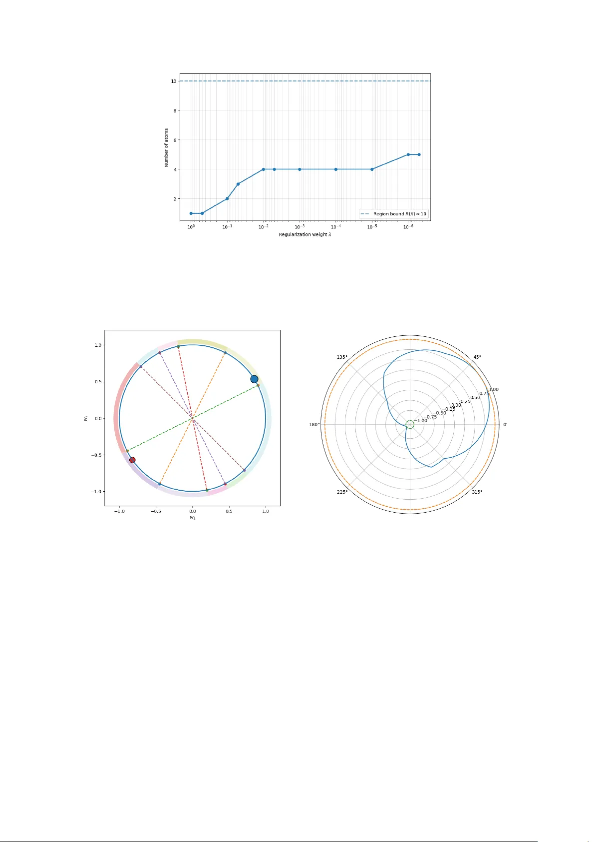
A Dual Certiﬁcate Approac h to Sparsit y in Inﬁnite-Width Shallo w Neural Net w orks Leonardo Del Grande ∗ , Christoph Brune ∗ , Marcello Carioni ∗ Abstract In this paper, we study total v ariation (TV)-regularized training of inﬁnite-width shallow ReLU neural net works, form ulated as a conv ex optimization problem o ver measures on the unit sphere. Our approac h lev erages the duality theory of TV-regularized optimization problems to establish rigorous guarantees on the sparsity of the solutions to the training problem. Our analysis further characterizes how and when this sparsity p ersists in a low noise regime and for small regularization parameter. The key observ ation that motiv ates our analysis is that, for ReLU activ ations, the asso ciated dual certiﬁcate is piecewise linear in the weigh t space. Its linearity regions, which w e name dual regions, are determined by the activ ation patterns of the data via the induced hyperplane arrangement. T aking adv an tage of this structure, we prov e that, on each dual region, the dual certiﬁcate admits at most one extreme v alue. As a consequence, the supp ort of an y minimizer is ﬁnite, and its cardinalit y can b e b ounded from ab ov e by a constant dep ending only on the geometry of the data- induced hyperplane arrangement. Then, we further inv estigate suﬃcien t conditions ensuring uniqueness of suc h sparse solution. Finally , under a suitable non-degeneracy condition on the dual certiﬁcate along the b oundaries of the dual regions, we prov e that in the presence of low lab el noise and for small regularization parameter, solutions to the training problem remain sparse with the same num ber of Dirac deltas. A dditionally , their lo cation and the amplitudes con verge, and, in case the lo cations lie in the interior of a dual region, the conv ergence happ ens with a rate that dep ends linearly on the noise and the regularization parameter. 1 In tro duction T w o-la yer neural net works with K neur ons are parametrized functions F c,w,b : R d → R deﬁned as F c,w,b ( x ) = K X i =1 c i σ ( ⟨ w i , x ⟩ + b i ) , (1.1) where σ : R → R is the so-called activation function , while c i ∈ R and w i ∈ R d are the weigh ts for the output and hidden lay ers of the net work, and b i ∈ R are the biases. F ollo wing the approac h in [ 2 , 22 ] one can consider the formal limit for K → + ∞ , i.e. when the num b er of neurons tends to inﬁnity and replace the sum in (1.1) b y the in tegration ov er a measure taking v alues on the space of weigh ts and biases. In particular, one deﬁnes F µ ( x ) = Z Θ σ ( ⟨ w , x ⟩ + b ) dµ ( w , b ) (1.2) where ( w , b ) ∈ Θ and µ ∈ M ( Θ ) . Problem (1.2) extends (1.1) since by c ho osing measures µ of the form µ = P N i =1 c i δ ( w i ,b i ) one reco vers instances of (1.1) . Moreov er, despite b eing inﬁnite- dimensional it is con vex in the space of measures (1.2) , allowing for insigh ts facilitated by the 2020 Mathematics Sub ject Classiﬁcation: 46A55, 49K27, 49N15, 49Q22, 52A40, 54E35 Keyw ords: conv ex optimization, Dirac deltas, duality , neural netw orks, regions, sparsity , stabilit y ∗ Departmen t of Applied Mathematics, Universit y of T wen te, 7500AE Enschede, The Netherlands ( l.delgrande@utwente.nl , c.brune@utwente.nl , m.c.carioni@utwente.nl ) 1 to ols of conv ex analysis (see for instance [ 9 ]). As often considered in the av ailable literature, the bias b is reabsorbed into the weigh t w b y identifying x = ( x, 1) and w = ( w , b ) , allo wing for a more compact representation F µ ( x ) = Z Θ σ ( ⟨ w , x ⟩ ) dµ ( w ) . In this work, we consider p ositiv ely 1 -homogeneous activ ation functions σ : R → R and, in particular, we often restrict our attention to the ReLU activ ation function deﬁned as σ ( z ) = max { 0 , z } for z ∈ R . Due to such 1 -homogeneity , since σ ( ⟨ w , x ⟩ ) = | w | σ ( ⟨ w / | w | , x ⟩ ) and rescaling the measure µ one can, without loss of expressivit y for F µ , consider measures taking v alues on the sphere, that is Θ = S d − 1 . Suc h a c hoice is also conv enien t, since the compactness of the parameter space allows for w ell-p osed v ariational problems in the space of measures. W e will mak e the choice Θ = S d − 1 throughout this pap er. A ccording to the previous considerations, given a collection of input/output pairs ( x j , y j ) n j =1 for n ∈ N , a typical training problem taking v alues in the space of measures M ( S d − 1 ) can b e deﬁned as min µ ∈ M ( S d − 1 ) 1 2 n X j =1 | F µ ( x j ) − y j | 2 + λ ∥ µ ∥ TV , (1.3) where ∥ µ ∥ TV is the total v ariation norm, deﬁned as ∥ µ ∥ TV = sup  Z φ ( x ) dµ ( x ) : φ ∈ C ( S d − 1 ) such that ∥ φ ∥ ∞ ⩽ 1  . (1.4) In this case, the total v ariation norm acts as a regularizer (whose in tensity is regulated b y λ ). In particular, it has the goal of enforcing sparsity in the solution. This means selecting solutions that are made of a linear combination of Dirac deltas, thus recov ering a classical neural netw ork (with a ﬁnite n umber of neurons). In the regime λ ≪ 1 , problem (1.3) approac hes an in terp olation problem, in whic h the data ﬁdelity term eﬀectively acts as a hard constraint. F ormally , one recov ers the constrained form ulation min µ ∈ M ( S d − 1 ) ∥ µ ∥ TV sub jected to F µ ( x j ) = y j ∀ j. (1.5) W e also remark that total v ariation norm regularization allows to deﬁne a natural representation costs for inﬁnite-width shallow neural netw orks op ening the wa y to the analysis of appro ximation capabilities of shallow neural net works. In deed, for f ∈ L 1 ( S d − 1 ) one can deﬁne ∥ f ∥ B ( S d − 1 ) = inf n ∥ µ ∥ TV : µ ∈ M ( S d − 1 ) , F µ ( x ) = f ( x ) for a.e. x ∈ S d − 1 o , that can b e seen as a representation cost in inﬁnite-width regimes. In analogy with foundational w orks by Barron [ 3 , 4 ], the quantit y ∥ f ∥ B ( S d − 1 ) is also named Barron norm and Barron functions are those functions f ∈ L 1 ( S d − 1 ) suc h that ∥ f ∥ B ( S d − 1 ) < ∞ (see for instance [ 21 ]). Man y imp ortan t works hav e carried out diﬀeren t asp ects of such analysis related either to the study of the representation cost or the appro ximation p o wer of Barron functions [ 18 , 21 , 22 , 23 , 26 , 34 , 38 , 40 ]. 1.1 Sparse guaran tees in inﬁnite-width limit of neural net works: state of the art and sup er-resolution theory It is a natural question to ask under which assumptions solutions of problem (1.3) and (1.5) are sparse, namely their minimizers are made of linear combinations of Dirac deltas of the form µ = N X i =1 c i δ w i . (1.6) 2 As highlighted in [ 6 ] in the context of Repro ducing Kernel Banach Spaces (RKBS), a ﬁrst, partial answ er is provided by so-called representer theorems [ 7 , 8 ]. In particular, when choosing the regularizer R ( µ ) = ∥ µ ∥ T V and assuming that the weigh t space Θ is compact, general representer theorems for inﬁnite-dimensional conv ex optimization problems guaran tee the existence of at least one solution of the form (1.6) , with the num b er of atoms b ounded by N ⩽ n . Such sparsity results hav e b een established in v arious training frameworks [ 5 , 6 , 35 , 36 ]. How ever, empirical evidence suggests that sparsity is not merely an existence prop erty: in practice, all minimizers often app ear to b e sparse even when multiple solutions exist. This naturally raises the question of whether all solutions are sparse. While this question remains largely unexplored in the machine learning literature with few exceptions [ 15 , 32 ], it has been studied in depth in the context of sup er-resolution, where similar problems are form ulated as conv ex optimization problems o ver spaces of measures. In this context, the prop ert y of having unique and sparse solutions is t ypically referred to as exact r e c onstruction . F oundational results [ 11 , 14 , 39 ] identify precise conditions under which exact reconstruction holds for TV-regularized interpolation problems with F ourier constrain ts. These results typically rely on dualit y arguments, where the key to ol is the construction of dual certiﬁcates η , i.e. dual v ariables that certify optimalit y and sparsit y of the primal solution by satisfying the asso ciated ﬁrst order optimalit y conditions [ 25 ]. Bey ond exact reco very , a substan tial bo dy of w ork has fo cused on sparse stabilit y , namely the robustness of sparsity under p erturbations of the problem. In this setting, one seeks conditions ensuring that the sparsit y of the solution p ersists when the regularization parameter λ v aries, and the data and lab els are con taminated b y noise. A series of inﬂuen tial w orks [ 16 , 19 , 20 , 37 ] has shown that sparse stabilit y is go verned b y non-degeneracy prop erties of the dual certiﬁcate asso ciated with the optimization problem. More precisely , stability holds when the dual certiﬁcate saturates its extreme v alues on the supp ort of the underlying sparse measure and exhibits a strict second order b ehavior there, namely lo cal strong concavit y (or con vexit y , dep ending on the sign con ven tion). These conditions preven t the creation or annihilation of atoms under small p erturbations. 1.2 Con tributions of the pap er In this pap er, we study sparsity prop erties of b oth problems (1.3) and (1.5) in the case of the ReLU activ ation function. Our analysis follows a duality-based approach, drawing on classical to ols from optimization in the space of measures and sup er-resolution techniques discussed in the previous part of the introduction. Dualit y metho ds play a central role in inﬁnite-dimensional optimization and in the analysis of sparse representations. Nev ertheless, their systematic use to establish sparsity guarantees for inﬁnite-width neural n et works remains largely unexplored. W e note, how ever, that dualit y techniques hav e app eared in the context of Barron spaces [ 41 ] and in certain ﬁnite-dimensional settings [ 29 ]. W e b egin our analysis by proving that every solution of b oth problems is sparse, and that the num b er of Dirac deltas in any minimizer is uniformly b ounded from ab ov e by a quan tity dep ending only on the ambien t dimension d and on the n umber of data p oin ts n . The k ey observ ation underlying our results is that the dual certiﬁcate associated with the problems can b e written in the explicit form η ( w ) = n X i =1 p i σ ( ⟨ w , x i ⟩ ) , p i ∈ R , w ∈ S d − 1 . When σ is the ReLU activ ation function, η coincides with the restriction to the sphere S d − 1 of a piecewise linear function. More precisely , its linearity regions are determined b y the intersection of the half-spaces { w : ⟨ w , x i ⟩ > 0 } and { w : ⟨ w , x i ⟩ < 0 } , referred to as dual r e gions , and η c hanges slope precisely across their common b oundaries  w : ⟨ w , x j ⟩ = 0  . Due to the geometry of the sphere, this observ ation allo ws us to conclude that in the in terior of each dual region, η ac hieves maximum and minim um in at most one p oint. Moreov er, at the 3 common b oundary of the regions (determined by the v anishing of the scalar pro ducts ⟨ w , x i ⟩ ), a similar analysis can also b e p erformed. Since, b y optimalit y conditions, the extreme v alues of the dual certiﬁcates determine the supp ort of the minimizers, one can then infer the sparsity of the minimizers. A dditionally , b y combinatorial arguments in volving the coun ting of non-empt y dual regions, one can also obtain an upp er b ound on the num b er of Dirac deltas constituting the minimizers. It is important to emphasize that the sparsit y of minimizers alone do es not imply uniqueness. In Section 3.3, we in tro duce suﬃcien t conditions guaran teeing the uniqueness of the minimizer. These conditions rely on tw o key prop erties: ﬁrst, given a sparse measure of the form (1.6) , the asso ciated dual certiﬁcate for problems (1.3) and (1.5) attains the extreme v alues | η ( w ) | = 1 exactly at the supp ort points w i ; second, the corresp onding neural netw ork ev aluations at the data p oints, namely R S d − 1 σ ( ⟨ w , x j ⟩ )d µ ( w ) , are linearly indep endent. In this section w e provide suﬃcien t conditions that guaran tee such linear indep endence. Finally , Section 4 is devoted to the analysis of sparse stabilit y for problem (1.5) . More precisely , w e sho w that, under suitable assumptions on the dual certiﬁcate and for suﬃcien tly small regularization parameters and noise lev els in the lab els, the sparsit y of the solution is preserv ed, with the same n umber of Dirac deltas. Moreo ver, the w eights c i and w i of the minimizer of the p erturb ed problem con verge to the w eights of the unp erturb ed one. As discussed in Section 1.1, a key ingredient for sparse stabilit y is the non-degeneracy of the dual certiﬁcate asso ciated with problem (1.5) . While this remains true in our setting, the piecewise linear structure of the dual certiﬁcate leads to non- degeneracy conditions with an explicit characterization. In particular, when a Dirac delta lies in the interior of a dual region, no additional non-degeneracy condition is required. In contrast, when a Dirac delta is lo cated at the b oundary of a region where the dual certiﬁcate is non-diﬀerentiable, the non-degeneracy is characterized by sign conditions on the (distributional) deriv ativ e of the dual certiﬁcate. Finally , in the case where the supp ort p oints w i lie in the in terior of a dual region, we establish quan titative conv ergence rates for the weigh ts of the minimizer of the p erturb ed problem. More precisely , under suitable linear indep endence assumptions on b oth the neural netw ork ev aluations at the data points and their deriv ativ es, w e prov e that    c i λ,ζ − c i 0    = O ( λ ) ,    w i λ,ζ − w i 0    = O ( λ ) , as λ → 0 and the noise ζ → 0 with ∥ ζ ∥ ⩽ α λ . 2 Notations and preliminaries 2.1 TV-regularized optimization in the space of measures In this section, w e review to ols of optimization in the space of measures we are going to use in the rest of the pap er. W e denote by M ( X ) the Banach space of ﬁnite signed Radon measures on a compact set X ⊂ R d , endo wed with the total v ariation norm. F or any Radon measure µ deﬁned on X , we also denote its supp ort by Supp ( µ ) . W e will consider TV-regularized optimization problems in the space of measures (commonly known as BLASSO [ 1 ]) that will b e written as inf µ ∈ M ( X ) 1 2 ∥ K µ − y ζ ∥ 2 Y + λ ∥ µ ∥ TV , where Y is a separable Hilb ert space, y ζ ∈ Y , K : M ( X ) → Y is a weak*-to-strong con tinuous linear op erator and λ is a p ositiv e parameter. Suc h problems are p opular as inv erse problems in the space of measures with applications to signal pro cessing [ 11 ], sup er-resolution in microscop y [ 17 ], sensor placement [ 33 ], and many others. Often, the measurement y ζ is a noisy p erturbation 4 of a ground truth signal y 0 , that is y ζ = y 0 + ζ . The goal is to reconstruct the optimal µ determining its sparsit y prop erties. In the formal limit ( ∥ ζ ∥ Y , λ ) → (0 , 0) , solutions to P λ ( y ζ ) con verge to solutions to the har d-c onstr aine d interpolation problem: inf µ ∈ M ( X ): K µ = y 0 ∥ µ ∥ TV . Existence of minimizers is guaranteed for all the problems (see for instance [ 12 , Section 3 ]). Moreo ver, this conv ergence can b e made rigorous as in the following classical result [ 27 , Theorem 3.5]. Prop osition 2.1. Supp ose that ther e exists µ ∈ M ( X ) such that K µ = y 0 . Consider se quenc es ζ n ∈ Y and λ n > 0 such that ∥ ζ n ∥ Y → 0 , λ n → 0 , ∥ ζ n ∥ 2 Y λ n → 0 as n → ∞ . Then, any se quenc e of minimizers of inf µ ∈ M ( X ) 1 2 ∥ K µ − y ζ n ∥ 2 Y + λ n ∥ µ ∥ TV has a we ak* c onver ging subse quenc e and e ach limit is a solution to P 0 ( y 0 ) . In p articular, if P 0 ( y 0 ) has a unique minimizer, then the whole se quenc e c onver ges we ak* to it. 2.1.1 Dualit y theory and optimalit y conditions A crucial source of information for minimizers of P λ ( y ζ ) and P 0 ( y 0 ) is given by resp ectiv e dual problems and optimality conditions. The dual problem associated with P λ ( y ζ ) (cf. [ 20 , 24 ]) is max p ∈ Y : ∥ K ∗ p ∥ ∞ ⩽ 1 ⟨ y ζ , p ⟩ − λ 2 ∥ p ∥ 2 Y , ( D λ ( y ζ ) ) while the dual problem asso ciated with P 0 ( y 0 ) is sup p ∈ Y : ∥ K ∗ p ∥ ∞ ⩽ 1 ⟨ y 0 , p ⟩ . ( D 0 ( y 0 ) ) Here K ∗ : Y → C ( X ) denotes the adjoin t op erator deﬁned by ⟨ K µ, p ⟩ Y = R X ( K ∗ p )( x ) dµ ( x ) for all µ ∈ M ( X ) and p ∈ Y , and ∥ · ∥ ∞ is the supremum norm on C ( X ) . Str ong duality holds b et ween P λ ( y ζ ) and D λ ( y ζ ) and the existence of µ λ,ζ ∈ M ( X ) solution to P λ ( y ζ ) and p λ,ζ ∈ Y solution to D λ ( y ζ ) , is equiv alen t to the following optimality conditions:    K ∗ p λ,ζ ∈ ∂ ∥ µ λ,ζ ∥ TV , − p λ,ζ = 1 λ ( K µ λ,ζ − y ζ ) . (2.1) Similarly , strong duality holds betw een P 0 ( y 0 ) and D 0 ( y 0 ) and the existence of µ 0 ∈ M ( X ) solution to P 0 ( y 0 ) and p 0 ∈ Y solution to D 0 ( y 0 ) , is equiv alent to the following optimality conditions: ( K ∗ p 0 ∈ ∂ ∥ µ 0 ∥ TV , K µ 0 = y 0 . (2.2) If η λ,ζ = K ∗ p λ,ζ and η λ,ζ ∈ ∂ ∥ µ λ,ζ ∥ TV , we call η λ,ζ a dual c ertiﬁc ate for µ λ,ζ with resp ect to P λ ( y ζ ) , since the optimality conditions (2.1) guaran tee that µ λ,ζ is a solution to P λ ( y ζ ) . Similarly , if η 0 = K ∗ p 0 and η 0 ∈ ∂ ∥ µ 0 ∥ TV , we call η 0 a dual c ertiﬁc ate for µ 0 with resp ect to P 0 ( y 0 ) , since the optimality conditions (2.2) guaran tee that µ 0 is a solution to P 0 ( y 0 ) . The solution p λ,ζ to D λ ( y ζ ) is unique, since this problem can b e reformulated as the Hilb ert pro jection of y ζ /λ on to the closed con vex set { p ∈ Y : ∥ K ∗ p ∥ ∞ ⩽ 1 } , c.f. [ 20 , Section 2.3]. On the other hand, the solution to D 0 ( y 0 ) is not unique. Among the dual certiﬁcates, an important role is play ed by the minimal-norm dual certiﬁcate deﬁned as follows. 5 Deﬁnition 2.2 (Minimal-norm dual certiﬁcate) . Suppose that there exists a solution to D 0 ( y 0 ) . Then the minimal-norm dual certiﬁcate is deﬁned as η 0 = K ∗ p 0 , where p 0 = argmin {∥ p ∥ Y : p ∈ Y is a solution to D 0 ( y 0 ) } . Since the sub diﬀerential of the total v ariation norm can b e characterized as ∂ ∥ µ ∥ TV =  φ ∈ C ( X ) : ∥ φ ∥ ∞ ⩽ 1 and Z X φ ( x ) dµ = ∥ µ ∥ TV  , one can deduce the following well-kno wn result that relates the extreme v alues of the dual certiﬁcate with the support of the optimal measure. Lemma 2.3. L et η 0 ∈ C ( X ) b e a dual c ertiﬁc ate for µ 0 . Then, µ 0 is a solution to P 0 ( y 0 ) and Supp( µ 0 ) ⊂ { x ∈ X : | η 0 ( x ) | = 1 } . Similarly, if η λ,ζ ∈ C ( X ) is the dual c ertiﬁc ate for µ λ,ζ . Then, µ λ,ζ is a solution to P λ ( y ζ ) and Supp( µ λ,ζ ) ⊂ { x ∈ X : | η λ,ζ ( x ) | = 1 } . 3 Dual regions and sparsity prop erties for inﬁnite-width neural net w orks The goal of this section is to construct and analyze dual certiﬁcates for inﬁnite-width neural net works with ReLU activ ation, and to infer sparsity prop erties of the minimizers. F rom now on, we will identify Y = R n and consider data p oints x j ∈ R d +1 , j = 1 , . . . , n . W e set y 0 := ( y 1 0 , . . . , y n 0 ) and y ζ := ( y 1 ζ , . . . , y n ζ ) . W e will consider b oth the interpolation problem without noise inf µ ∈ M ( S d − 1 ) ∥ µ ∥ TV sub jected to F µ ( x j ) = y j 0 ∀ j ( P 0 ( y 0 ) ) and the TV-regularized empirical loss where the lab els are p erturb ed as y j ζ = y j 0 + ζ j , with ζ = ( ζ 1 , . . . , ζ n ) ∈ R n , inf µ ∈ M ( S d − 1 ) 1 2 n X j =1 | F µ ( x j ) − y j ζ | 2 + λ ∥ µ ∥ TV . ( P λ ( y ζ ) ) W e recall that ∥ · ∥ TV denotes the total v ariation norm, deﬁned in (1.4) . Note that b y deﬁning the linear op erator K : M ( S d − 1 ) → R n as ( K µ ) j := F µ ( x j ) = Z S d − 1 σ ( ⟨ w , x j ⟩ )d µ ( w ) j = 1 , . . . , n, where σ ( z ) = ReLU ( z ) , w e obtain that P 0 ( y 0 ) has the form of a general hard-constrained TV-regularized problem P 0 ( y 0 ) inf µ ∈ M ( S d − 1 ): K µ = y 0 ∥ µ ∥ TV and P λ ( y ζ ) has the form of a general Tikhonov-t yp e regularized problem P λ ( y ζ ) inf µ ∈ M ( S d − 1 ) 1 2 ∥ K µ − y ζ ∥ 2 R n + λ ∥ µ ∥ TV , allo wing us to use the dual certiﬁcate theory dev elop ed in Section 2.1, provided K is weak*-to- strong contin uous. This is veriﬁed in the next easy lemma. 6 Lemma 3.1. The op er ator K : M ( S d − 1 ) → R n is we ak*-to-str ong c ontinuous. Mor e over, its adjoint K ∗ : R n → C ( S d − 1 ) is given by K ∗ p ( w ) = n X j =1 p j σ ( ⟨ w , x j ⟩ ) ∀ p ∈ R n . (3.1) Pr o of. The weak* contin uit y of K is immediate. In particular, since the co domain is ﬁnite- dimensional, K is weak*-to-strong contin uous. T o prov e the characterization of K ∗ it is enough to note that, for all µ ∈ M ( S d − 1 ) , it holds that Z S d − 1 K ∗ p d µ ( w ) = ⟨ K ∗ p, µ ⟩ = ( p, K µ ) R n = n X j =1 p j ( K µ ) j = n X j =1 p j Z S d − 1 σ ( ⟨ w , x j ⟩ )d µ ( w ) = Z S d − 1 n X j =1 p j σ ( ⟨ w , x j ⟩ )d µ ( w ) = ⟨ n X j =1 p j σ ( ⟨ w , x j ⟩ ) , µ ⟩ . W e now specialize, for the sake of clarity in the rest of the pap er, the abstract dual problems from the previous section to the present ReLU setting. In particular, using (3.1) , the dual of the in terp olation problem P 0 ( y 0 ) b ecomes sup p ∈ R n ⟨ p, y 0 ⟩ sub ject to sup w ∈ S d − 1    n X j =1 p j σ ( ⟨ w , x j ⟩ )    ⩽ 1 . ( D 0 ( y 0 ) ) An y maximizer p 0 of D 0 ( y 0 ) yields a dual certiﬁcate η 0 ( w ) := K ∗ p 0 ( w ) = P n j =1 p j 0 σ ( ⟨ w , x j ⟩ ) . Instead, the dual of P λ ( y ζ ) b ecomes sup p ∈ R n ⟨ y ζ , p ⟩ − λ 2 ∥ p ∥ 2 sub ject to sup w ∈ S d − 1    n X j =1 p j σ ( ⟨ w , x j ⟩ )    ⩽ 1 . ( D λ ( y ζ ) ) Giv en the maximizer p λ,ζ of D λ ( y ζ ) , w e deﬁne the dual certiﬁcate η λ,ζ ( w ) := K ∗ p λ,ζ ( w ) = P n j =1 p j λ,ζ σ ( ⟨ w , x j ⟩ ) . Since Y = R n , the dual problem D λ ( y ζ ) admits a (unique) maximizer for ev ery λ > 0 . F or D 0 ( y 0 ) , maximizers may b e not unique; w e will consider the minimal-norm one when needed. Moreov er, by the following standard result (see for example [ 20 , Prop osition 1]), the dual certiﬁcates con verge uniformly in the noiseless regime as the regularization parameter v anishes. Prop osition 3.2 (Conv ergence of the dual certiﬁcates) . L et p λ, 0 b e the unique solution to D λ ( y 0 ) . L et p 0 b e the solution with minimal-norm of D 0 ( y 0 ) . Then, lim λ → 0 + ∥ η λ, 0 − η 0 ∥ ∞ = 0 . Pr o of. By deﬁnition and (3.1), for ev ery w ∈ S d − 1 w e ha ve η λ, 0 ( w ) − η 0 ( w ) = n X j =1  p j λ, 0 − p j 0  σ ( ⟨ w , x j ⟩ ) . Hence, ∥ η λ, 0 − η 0 ∥ ∞ = sup w ∈ S d − 1       n X j =1  p j λ, 0 − p j 0  σ ( ⟨ w , x j ⟩ )       7 ⩽ n X j =1 | p j λ, 0 − p j 0 | sup w ∈ S d − 1 σ ( ⟨ w , x j ⟩ ) . Since σ ( z ) = max { 0 , z } and sup ∥ w ∥ =1 ⟨ w , x j ⟩ = ∥ x j ∥ , w e obtain sup w ∈ S d − 1 σ ( ⟨ w , x j ⟩ ) = ∥ x j ∥ . If w e let C := max 1 ⩽ j ⩽ n ∥ x j ∥ < ∞ , then ∥ η λ, 0 − η 0 ∥ ∞ ⩽ C n X j =1 | p j λ, 0 − p j 0 | = C ∥ p λ, 0 − p 0 ∥ 1 . By [ 20 , Prop osition 1], p λ, 0 → p 0 in R n , implying ∥ p λ, 0 − p 0 ∥ 1 → 0 as λ → 0 . Therefore, it holds lim λ → 0 + ∥ η λ, 0 − η 0 ∥ ∞ = 0 as desired. 3.1 Dual regions Giv en v ectors { x 1 , . . . , x n } ⊂ R d (assume x i  = 0 ), we consider the h yp erplane arrangemen t H i := { w ∈ R d : ⟨ w , x i ⟩ = 0 } , i = 1 , . . . , n, together with the associated op en half-spaces A 1 i := { w ∈ R d : ⟨ w , x i ⟩ > 0 } , A 0 i := { w ∈ R d : ⟨ w , x i ⟩ < 0 } . A binary vector π = ( π 1 , . . . , π n ) ∈ { 0 , 1 } n prescrib es, for each i , a sign pattern for the scalars ⟨ w , x i ⟩ and thus determines the in tersection R π := n \ i =1 A π i i . W e call the (p ossibly empty) op en subset R π ⊂ R d a dual r e gion . The term “dual” emphasizes that these regions live in the weight sp ac e ( w -v ariable), in contrast with the more common “linear region” decomp ositions in input sp ac e ( x -v ariable). In tersections of this type are w ell known in the literature of neural netw orks analysis. W e refer, for example, to the “sectors” of [ 30 , 15 ], the linear regions studied in [ 31 ], and the activ ation regions introduced in [ 28 ]. F or instance, see Figure 1, which depicts the spherical dual regions R π ∩ S 1 for d = n = 2 . Deﬁnition 3.3 (Dual region) . Given π = ( π 1 , . . . , π n ) ∈ { 0 , 1 } n , w e call a dual r e gion asso ciated with π R π := n \ i =1 A π i i . It is well known from classical results on linearly separable dic hotomies/central hyperplane ar- rangemen ts (V apnik–Chervonenkis dimension theory) that the num b er of distinct binary vectors π suc h that the dual region R π is non-empty is at most 2 P d − 1 k =0  n − 1 k  ; equality holds when the h yp erplanes { H i } n i =1 are in general p osition (see, e.g., [ 13 , Theorem 1]). In particular, thanks to the binomial theorem, w e obtain that there are at most 2 n p ossible combinations (indep endent of d ) if and only if n ⩽ d . Instead, if n > d , then, one can b ound the num b er of these com binations b y O ( n d ) (refer to [ 28 , Prop osition 6], [ 30 , Chapter 4]). In what follo ws, w e will denote by Θ the set of binary vectors π such that the region R π is non-empty . Our analysis will necessarily deal with the b oundary of dual regions. T o capture optimality on these sets, w e will in tro duce the concept of higher c o dimension dual regions, obtained b y allowing 8 H 1 H 2 x 1 x 2 R (1 , 1) R (1 , 0) R (0 , 1) R (0 , 0) Figure 1: Dual regions on S 1 induced by tw o inputs ( d = n = 2 ). some of the deﬁning inequalities to b ecome equalities. This yields a natural stratiﬁcation of the w eight space into op en cells of v arying co dimension, which will b e crucial for our study . W e also remark that the need for such structures has already b een noted in [ 28 , 30 ]. Consider the index set I := { 1 , . . . , n } and, for k ⩽ n , let J k = { j 1 , . . . , j k } ⊂ I . W e aim to deﬁne regions of co dimension n − k that b elong to the topological b oundary of a giv en region R π . Deﬁnition 3.4 (Higher–co dimension dual regions) . Let π ∈ { 0 , 1 } n and R π b e as in Deﬁni- tion 3.3. F or J k ⊂ I with | J k | = k , we deﬁne the J k -stratum of R π as follows: R J k π :=  \ j ∈ J k A π j j  ∩  \ z ∈ I \ J k H z  , where H z := { w ∈ R d : ⟨ w , x z ⟩ = 0 } . By con ven tion, R I π = R π . The set R J k π lies in L J k := T z ∈ I \ J k H z , which has co dimension at most | I \ J k | = n − k in R d (and equals n − k if the normals { x z } z ∈ I \ J k are linearly indep endent). Similarly to the codimension zero case, we denote b y Θ J k := { π ∈ { 0 , 1 } n : R J k π  = ∅} the set of sign patterns for whic h the stratum R J k π is non-empty . F or simplicity , we are going to call R J k π again a dual region. Remark 3.5 (Boundary stratiﬁcation) . Let R J k π denote the closure of R J k π in the relativ e top ology of L J k . Here and b elo w, ∂ denotes the b oundary taken in the same relative top ology . Note that the topological b oundary of a region R π can b e simply rewritten as ∂ R π = [ J n − 1 ⊂ I R J n − 1 π , that is, the union of the closures of its co dimension 1 faces. Lo wer dimensional strata are con tained in these closures. More generally , for k = 1 , . . . , n − 2 , the top ological b oundary of R J k π b ecomes: ∂ R J k π = [ J k − 1 ⊂ J k R J k − 1 π , where | J k − 1 | = k − 1 . 9 3.2 Sparse c haracterization and upp er b ounds on the n um b er of Dirac deltas The deriv ation of an exact reconstruction result for the interpolation hard-constrained problem P 0 ( y 0 ) is based on the b ehaviour of the dual certiﬁcate in the du al regions, determined by the input data { x 1 , . . . , x n } . F or this, it is crucial to choose the ReLU as activ ation function σ . First, it is easy to see that since σ ( z ) = ReLU( z ) , for every i = 1 , . . . , n , w e can write σ ( ⟨ w , x i ⟩ ) = π i ⟨ w , x i ⟩ for every w ∈ R π . (3.2) As a consequence the minimal-norm dual certiﬁcate can b e written as a linear function in eac h dual region R π as stated in the next lemma. When ⟨ w , x i ⟩ = 0 w e hav e σ ( ⟨ w , x i ⟩ ) = 0 ; b oundary cases will b e treated via the strata R J k π . Lemma 3.6. Given a binary ve ctor π , for every w ∈ R π , every dual c ertiﬁc ate η 0 c an b e r ewritten as η 0 ( w ) = n X i =1 p i 0 π i ⟨ w , x i ⟩ . Pr o of. The lemma follo ws directly from Lemma 3.1 and (3.2). In particular, every dual certiﬁcate η 0 ∈ C ( S d − 1 ) is the restriction to S d − 1 of a function that is linear on each cone R π and thus globally piecewise linear. This enables us to use the dual certiﬁcate theory summarized in Section 2.1 to obtain information ab out the supp ort of the minimizers of P 0 ( y 0 ) and P λ ( y ζ ) . Indeed, in the next lemma, w e use the piecewise linear structure of the dual certiﬁcate to show that the num b er of p oints where its absolute v alue ac hieves one is ﬁnite. Thanks to the optimalit y conditions in (2.2) , this will imply that the supp ort of the minimizers of P 0 ( y 0 ) is a discrete set (see Corollary 3.10). Lemma 3.7. L et p 0 b e a solution to D 0 ( y 0 ) and let η 0 = K ∗ p 0 b e a dual c ertiﬁc ate. Fix π ∈ { 0 , 1 } n , J k ⊂ I with | J k | = k , and set z 0 := X i ∈ J k p i 0 π i x i , ˜ z 0 := P L J k z 0 , wher e P L J k denotes the ortho gonal pr oje ction onto L J k . If ther e exists w 0 ∈ R J k π ∩ S d − 1 such that | η 0 ( w 0 ) | = 1 , then ˜ z 0  = 0 and w 0 = sign( η 0 ( w 0 )) ˜ z 0 ∥ ˜ z 0 ∥ . Mor e over, | η 0 ( w ) | < 1 for every w ∈  R J k π ∩ S d − 1  \ { w 0 } . Pr o of. First, note that on R J k π ∩ S d − 1 the dual certiﬁcate η 0 can b e written as η 0 ( w ) = X i ∈ J k p i 0 π i ⟨ w , x i ⟩ = ⟨ z 0 , w ⟩ , z 0 := X i ∈ J k p i 0 π i x i . Since w ∈ L J k , we also ha ve ⟨ z 0 , w ⟩ = ⟨ P L J k z 0 , w ⟩ = ⟨ ˜ z 0 , w ⟩ , where ˜ z 0 := P L J k z 0 . Assume there exists w 0 ∈ R J k π ∩ S d − 1 suc h that | η 0 ( w 0 ) | = 1 . Then ˜ z 0  = 0 (otherwise η 0 ≡ 0 on L J k ∩ S d − 1 ). By Cauch y–Sch warz, for every w ∈ L J k ∩ S d − 1 , | η 0 ( w ) | = |⟨ ˜ z 0 , w ⟩| ⩽ ∥ ˜ z 0 ∥ , with equality if and on ly if w = ± ˜ z 0 / ∥ ˜ z 0 ∥ . Since | η 0 ( w 0 ) | = 1 , necessarily ∥ ˜ z 0 ∥ ⩾ 1 , and equality in Cauch y–Sch warz implies w 0 = sign( η 0 ( w 0 )) ˜ z 0 ∥ ˜ z 0 ∥ . 10 T o prov e uniqueness inside R J k π ∩ S d − 1 , supp ose that | η 0 ( ¯ w ) | = 1 for some ¯ w ∈ R J k π ∩ S d − 1 . Then b y the same argumen t ¯ w = ± ˜ z 0 / ∥ ˜ z 0 ∥ . The choice ¯ w = − w 0 is incompatible with b elonging to R J k π . Indeed, for any index i ∈ J k with π i = 1 we hav e ⟨ w 0 , x i ⟩ ⩾ 0 on the closure, hence ⟨− w 0 , x i ⟩ ⩽ 0 , which would force − w 0 to lie in the opp osite half-space (or on the h yp erplane), con tradicting ¯ w ∈ R J k π unless all such scalar pro ducts v anish (which cannot o ccur if | η 0 ( w 0 ) | = 1 ). Therefore ¯ w = w 0 , and the statemen t follows. Remark 3.8. Note that the previous lemma put constraints on the p oin ts where the absolute v alue of the dual certiﬁcate reaches one. In particular, under the assumption of the previous prop osition it also holds that | η 0 ( w ) | < 1 for every w ∈ S J k − 1 ⊂ J k R J k − 1 π ∩ S d − 1 . Moreov er, if w 0 b elongs to a region of 0 -co dimension, that is if k = n , then ˜ z 0 = z 0 . A similar statement holds for the dual certiﬁcate asso ciated with P λ ( y ζ ) . Lemma 3.9. L et p λ,ζ ∈ R n b e the solution to D λ ( y ζ ) and let η λ,ζ = K ∗ p λ,ζ b e the dual c ertiﬁc ate for P λ ( y ζ ) . Fix π ∈ { 0 , 1 } n , J k ⊂ I with | J k | = k , and set z λ,ζ = X i ∈ J k p i λ,ζ π i x i , ˜ z λ,ζ = P L J k z λ,ζ . (3.3) If ther e exists w λ,ζ ∈ R J k π ∩ S d − 1 such that | η λ,ζ ( w λ,ζ ) | = 1 , then ˜ z λ,ζ  = 0 and w λ,ζ = sign( η λ,ζ ( w λ,ζ )) ˜ z λ,ζ ∥ ˜ z λ,ζ ∥ . (3.4) Mor e over, | η λ,ζ ( w ) | < 1 for every w ∈ ( R J k π ∩ S d − 1 ) \ { w λ,ζ } . F rom the previous lemmas it follo ws directly the mentioned sparse c haracterization of minimizers of P 0 ( y 0 ) and P λ ( y ζ ) . Theorem 3.10 (Sparsity of minimizers) . The fol lowing two statements hold: • Ther e exists N ∈ N such that al l the solutions to P 0 ( y 0 ) ar e of the form µ 0 = N X i =1 c i 0 δ w i 0 , wher e c i 0 ∈ R and w i 0 = sign ( η 0 ( w 0 )) z 0 | z 0 | with z 0 = P i ∈ J k p i 0 π i x i for some binary ve ctor π and J k ⊂ I . • Ther e exists M ∈ N such that al l the solutions to P λ ( y ζ ) ar e of the form µ λ,ζ = M X i =1 c i λ,ζ δ w i λ,ζ , wher e c i λ,ζ ∈ R and w i λ,ζ = sign ( η λ,ζ ( w i λ,ζ )) z λ,ζ ∥ z λ,ζ ∥ with z λ,ζ = P i ∈ J k p i λ,ζ π i x i for some binary ve ctor π and J k ⊂ I . Pr o of. The pro of follows from Lemma 3.7 and Lemma 3.9 together with the optimalit y conditions for P 0 ( y 0 ) and P λ ( y ζ ) summarized in Lemma 2.3. 11 F rom a rough estimate one can upp er b ound b oth N and M (w e denote by N max a common upp er b ound depending only on n and d ) in the previous theorem by N max ⩽ 3 n . (3.5) This is obtained as all possible wa ys to c ho ose the sign of eac h scalar pro duct ⟨ w , x i ⟩ for i = 1 , . . . , n ( ⟨ w , x i ⟩ > 0 , ⟨ w , x i ⟩ < 0 or ⟨ w , x i ⟩ = 0 in corresp ondence with regions of higher co dimension). W e are coun ting the ternary activ ation patterns for eac h i ∈ { 1 , . . . , n } . Ho wev er, ﬁner estimates are p ossible, as describ ed in the remaining part of this subsection. Lemma 3.11. The absolute value of the dual c ertiﬁc ate η 0 (r esp. η λ,ζ ) for P 0 ( y 0 ) (r esp. P λ ( y ζ ) ) achieves its maximum in at most max 0 ⩽ k ⩽ n n k ! Ξ ( n − k , d − k ) p oints, wher e Ξ ( n − k , d − k ) denotes the numb er of non-empty r e gions induc e d in R d − k by an arr angement of n − k hyp erplanes and we use the c onvention that Ξ ( n − k , d − k ) = 0 when d − k < 0 . Pr o of. The pro of of the statemen t is the same for the in terp olation problem P 0 ( y 0 ) and for the training problem P λ ( y ζ ) . The pro of is based on the observ ation that if | η | is maximized at some p oin t in a given stratum R J k π for J k ⊂ I , then it cannot b e maximized at any other p oin t in lo wer dimensional strata R J k − 1 π for J k − 1 ⊂ J k . Moreov er, distinct strata corresp ond to disjoint ternary patterns, so maximizers are coun ted by enumerating all the strata. In particular, we ha ve  n k  w ays of c ho osing k ’s x i suc h that ⟨ x i , w ⟩ = 0 . This in tersection of planes determines a set of dimension R d − k . In suc h a set, w e are allow ed to c ho ose the intersection of n − k h yp erplanes that leads to the factor Ξ ( n − k , d − k ) . Remark 3.12. The previous lemma giv es a sharp er estimate with respect to the rough b ound in (3.5). Indeed, since Ξ ( n − k , d − k ) ⩽ 2 n − k , then by the binomial theorem we obtain that max 0 ⩽ k ⩽ n n k ! Ξ ( n − k , d − k ) ⩽ max 0 ⩽ k ⩽ n n k ! 2 n − k ⩽ n X k =0 n k ! 2 n − k = 3 n Therefore, if n ⩽ d the b est b ound w e can get is max 0 ⩽ k ⩽ n n k ! 2 n − k that can b e estimated grossly by 3 n . Even if slightly more precise estimates can b e obtained, we will not enter into these details here. Instead, if n > d it holds that Ξ ( n − k , d − k ) ⩽ O (( n − k ) d − k ) . Hence, taking into account that Ξ ( n − k , d − k ) = 0 when d − k < 0 , it holds that max 0 ⩽ k ⩽ n n k ! Ξ ( n − k , d − k ) ⩽ max 0 ⩽ k ⩽ n n k ! O (( n − k ) d − k ) = max 0 ⩽ k ⩽ n n n − k ! O ( k d − ( n − k ) ) ⩽ max 0 ⩽ k ⩽ n n n − k ! O ( n d − ( n − k ) ) ⩽ n n − k ( n − k )! O ( n d − ( n − k ) ) ⩽ O ( n d ) . Note that this b ound, in the case n > d , is actually equal to O ( Ξ ( n, d )) , that is, prop ortional to the num b er of dual regions. This yields a sharp er estimate than the one provided in [ 15 ]. 12 3.3 Linear indep endence and uniqueness of the minimizers In the previous subsection we pro ved that both problems P 0 ( y 0 ) and P λ ( y ζ ) admit sparse minimizers and we provided an upp er b ound on the num b er of Dirac deltas in any such represen- tation. W e now address uniqueness. As common in the av ailable literature on TV-regularized optimization problems in the space of measures, uniqueness follows from a com bination of (i) a lo calization prop erty of the dual certiﬁcate and (ii) a linear indep endence condition on the measuremen t vectors { K δ w i } . W e provide suﬃcient conditions ensuring (ii) in our ReLU setting. W e caution that our conditions are lik ely not sharp and that a complete characterization lies b ey ond the scop e of this w ork. W e begin b y recalling sev eral deﬁnitions from linear algebra. Deﬁnition 3.13 (Hadamard product) . The Hadamard or entry-wise pro duct of t wo matrices M and N of the same dimension is deﬁned as M ⊙ N := ( M ij · N ij ) . W e will also need the deﬁnition of tr ansversal given for example in [ 10 ]. Deﬁnition 3.14 (T ransversal) . A transversal of an m × n matrix is a set of m en tries, one from eac h ro w and no t wo from the same column. W e also recall that the determinan t of a squ are matrix M = ( m ij ) ∈ R n × n can b e computed as det( M ) := X p ∈P n sign( p ) n Y i =1 m i,p ( i ) ! , where the sum is ov er all permutations p ∈ P n of n elements. Deﬁnition 3.15 (P ermanent) . Given a square matrix M = ( m ij ) ∈ R n × n , the p ermanent of M is deﬁned as p erm( M ) := X p ∈P n n Y i =1 m i,p ( i ) . Let µ 0 = P N i =1 c i 0 δ w i 0 with c i 0 ∈ R and w i 0 ∈ R π i for i = 1 , . . . , N . Let w 0 := ( w 1 0 , . . . , w N 0 ) . W e deﬁne the N × n ev aluation matrix K ( w 0 ) :=        σ ( ⟨ w 1 0 , x 1 ⟩ ) · · · σ ( ⟨ w 1 0 , x n ⟩ ) . . . · · · . . . . . . . . . . . . σ ( ⟨ w N 0 , x 1 ⟩ ) · · · σ ( ⟨ w N 0 , x n ⟩ )        =        π 1 1 ⟨ w 1 0 , x 1 ⟩ · · · π 1 n ⟨ w 1 0 , x n ⟩ . . . · · · . . . . . . . . . . . . π N 1 ⟨ w N 0 , x 1 ⟩ · · · π N n ⟨ w N 0 , x n ⟩        , where π i j := 1 ⟨ w i 0 ,x j ⟩ > 0 so that σ ( ⟨ w i 0 , x j ⟩ ) = π i j ⟨ w i 0 , x j ⟩ . Its i -th row is exactly the measurement v ector ( K δ w i 0 ) ⊤ ∈ R 1 × n . Moreov er, if we denote Π :=        π 1 1 · · · π 1 n . . . · · · . . . . . . . . . . . . π N 1 · · · π N n        , X :=        x 1 1 · · · x n 1 . . . · · · . . . . . . . . . . . . x 1 d · · · x n d        , W :=        w 1 0 , 1 · · · w N 0 , 1 . . . · · · . . . . . . . . . . . . w 1 0 ,d · · · w N 0 ,d        , where w i 0 = ( w i 0 , 1 , . . . , w i 0 ,d ) and x i = ( x i 1 , . . . , x i d ) then we can rewrite K ( w 0 ) = Π ⊙ W ⊤ X . In the following lemma we will prov e that { K δ w i 0 } N i =1 are linearly indep endent under certain assumptions on Π and supp osing that N ⩽ n . Note that such condition is necessary , since otherwise the vectors { K δ w i 0 } N i =1 cannot b e linearly indep enden t. 13 Lemma 3.16. L et µ 0 = P N i =1 c i 0 δ w i 0 with c i 0 ∈ R and w i 0 ∈ R π i , N ⩽ n . Supp ose that the fol lowing c onditions ar e satisﬁe d: i) Some N × N minor of Π , c al le d Π N , has ful l r ank; ii) perm ( Π N ) = | det( Π N ) | . Then, the ve ctors { K δ w i 0 } N i =1 ar e line arly indep endent. Pr o of. By the deﬁnition of K w e hav e to prov e that { σ ( ⟨ w i 0 , x 1 ⟩ ) , . . . , σ ( ⟨ w i 0 , x n ⟩ ) } N i =1 are linearly indep enden t. W e will equiv alen tly prov e that K ( w 0 ) has rank N , that is it has an N × N minor with nonzero determinan t. Let Π N b e an N × N minor of Π whic h is nonsingular by assumption i) , and let ( W ⊤ X ) N b e the corresp onding N × N minor of W ⊤ X (same rows and columns). Set B := ( W ⊤ X ) N , A := Π N ∈ { 0 , 1 } N × N . Then the corresp onding minor of K ( w 0 ) = Π ⊙ ( W ⊤ X ) is A ⊙ B and det( A ⊙ B ) = X p ∈P N sign( p ) N Y i =1 A i,p ( i ) B i,p ( i ) . By assumption i) , there exists at least one p ermutation ¯ p suc h that Q i A i, ¯ p ( i ) = 1 (a transv ersal of ones). Moreov er, by assumption ii) , or equiv alently p erm ( A ) = | det ( A ) | , all p ermutations p with Q i A i,p ( i ) = 1 hav e the same parity , hence the same sign sign ( p ) = s ∈ {± 1 } . F or those p , w e also hav e B i,p ( i ) = ⟨ w i 0 , x p ( i ) ⟩ > 0 , since A i,p ( i ) = 1 means ⟨ w i 0 , x p ( i ) ⟩ > 0 in the asso ciated dual region. Therefore, ev ery nonzero term in the expansion of det ( A ⊙ B ) has the same sign s and is strictly p ositiv e in magnitude, and in particular the term corresp onding to ¯ p is nonzero due to the fact that Q i A i, ¯ p ( i ) = 1 . Hence, det ( A ⊙ B )  = 0 , implying that K ( w 0 ) has rank N . Remark 3.17. Note that in the pro of we are using that the second assumption, that is p erm ( Π N ) = | det ( Π N ) | for 0 - 1 matrices, is equiv alent to all transversals of Π N , i.e. all p er- m utations p with Q N i =1 ( Π N ) i,p ( i ) = 1 , having the same parity . The previous lemma pro vides easy scenarios where the linear indep endence of { K δ w i 0 } N i =1 is ensured. F or example if Π N is a p erm utation matrix, then i ) and ii ) are automatically veriﬁed. T o the b est of our kno wledge, these conditions hav e not been explored in the literature. Extending this line of results is left for future research. W e are now ready to examine uniqueness for the sparse solutions to P 0 ( y 0 ) and P λ ( y ζ ) . W e ﬁrst treat the in terp olation problem P 0 ( y 0 ) , since the analysis for the training problem P λ ( y ζ ) follo ws the same strategy . Let µ 0 = P N i =1 σ i c i 0 δ w i 0 with c i 0 > 0 , σ i ∈ {− 1 , +1 } and w i 0 ∈ S d − 1 satisfy the hard constrain t K µ 0 = y 0 of P 0 ( y 0 ) . If µ 0 is a minimizer, the dual certiﬁcate η 0 satisﬁes η 0 ( w i 0 ) = σ i b y Lemma 2.3. T o conclude uniqueness, w e require that | η 0 | attains its maximum 1 only at the atoms { w i 0 } N i =1 and that the measuremen ts { K δ w i 0 } N i =1 are linearly indep endent (ensured by ( i ) , ( ii ) in Lemma 3.16). Theorem 3.18. L et µ 0 = P N i =1 c i 0 σ i δ w i 0 b e such that y 0 = K µ 0 , with c i 0 > 0 , σ i ∈ {− 1 , 1 } and w i 0 ∈ R π i for al l i = 1 , . . . , N . L et η 0 b e the dual c ertiﬁc ate for µ 0 , and supp ose that { K δ w i 0 } N i =1 ar e line arly indep endent and (LC) | η 0 ( w ) | < 1 for al l w ∈ S d − 1 \ { w 1 0 , . . . w N 0 } . Then, µ 0 is the unique solution to P 0 ( y 0 ) . Pr o of. The pro of follows directly by applying [ 12 , Lemma 4.5]. 14 A verbatim statement holds for the training problem when the dual certiﬁcate for P λ ( y ζ ) plays the role of η 0 . Theorem 3.19. L et µ λ,ζ = P N i =1 c i λ,ζ σ i δ w i λ,ζ , with c i λ,ζ > 0 , σ i ∈ {− 1 , 1 } and w i λ,ζ ∈ R π i for al l i = 1 , . . . , N . L et η λ,ζ b e the dual c ertiﬁc ate for µ λ,ζ , and supp ose that { K δ w i λ,ζ } N i =1 ar e line arly indep endent and ( g LC) | η λ,ζ ( w ) | < 1 for al l w ∈ S d − 1 \ { w 1 λ,ζ , . . . w N λ,ζ } . Then, µ λ,ζ is the unique solution to P λ ( y ζ ) . Remark 3.20. The lo calization condition (LC), together with the optimality conditions ensures that the dual certiﬁcate is maximized only at the Dirac deltas lo cations { w i 0 } N i =1 (and similarly for η λ,ζ ). By Lemmas 3.7–3.9, for each dual region R J k π ∩ S d − 1 the function | η | has at most one p oin t where it can p ossibly attain its maximum (when the region is nonempt y). In particular, in the interior of a region there cannot b e tw o distinct maximizers. Consequen tly , to chec k the lo calization condition it is not necessary to control | η | ev erywhere on S d − 1 but it suﬃces to insp ect the ﬁnite collection of c andidate maximizers and verify that | η | = 1 only on the supp ort of the sparse measure, while all the remaining candidates satisfy | η | < 1 . The size of this candidate set is ﬁnite and is b ounded as in Lemma 3.11 and Remark 3.12. 4 Sparse stabilit y for noisy lab els under regularization In this section, we aim to sho w that for suﬃciently small regularization parameter λ and in a lo w noise regime, every solution to P λ ( y ζ ) has the same num b er of Dirac deltas as the (unique) solution to P 0 ( y 0 ) . Moreov er, the lo cations and w eights are contin uous p erturbations of those of µ 0 as ( λ, ζ ) → (0 , 0) within the admissible set N α,λ 0 deﬁned b elow. Such results are t ypically referred to as exact supp ort r e c overy [ 20 ]. W e consider the following set of admissible parameters/noise levels for λ 0 > 0 and α > 0 : N α,λ 0 = { ( λ, ζ ) ∈ R + × R n : 0 < λ ⩽ λ 0 and ∥ ζ ∥ ⩽ αλ } . This set was introduced in [ 20 ] and describ es the regime in which one exp ects exact supp ort reco very . Let us also deﬁne the extended supp ort as in tro duced in [ 20 ]. Deﬁnition 4.1 (Extended supp ort [ 20 ]) . Let µ 0 ∈ M ( S d − 1 ) b e such that y 0 = K µ 0 and let η 0 ∈ C ( S d − 1 ) denote the minimal-norm dual certiﬁcate asso ciated with P 0 ( y 0 ) . The extended supp ort of the measure µ 0 is deﬁned as Ext( µ 0 ) := n w ∈ S d − 1 : | η 0 ( w ) | = 1 o . Note that Supp ( µ 0 ) ⊂ Ext ( µ 0 ) b y Lemma 2.3. Analogously , for µ λ,ζ with dual certiﬁcate η λ,ζ , set Ext ( µ λ,ζ ) := { w ∈ S d − 1 : | η λ,ζ ( w ) | = 1 } . W e now recall a fundamental result, [ 20 , Lemma 1 ], regarding the supp ort of solutions to P λ ( y ζ ) in the low noise regime and for small regularization parameters. Lemma 4.2. L et p 0 b e the minimal norm solution to D 0 ( y 0 ) , p λ,ζ the solution to D λ ( y ζ ) and µ λ,ζ ∈ M ( S d − 1 ) any solution to P λ ( y ζ ) . Given ε, δ > 0 , ther e exist α > 0 , λ 0 > 0 such that, for al l ( λ, ζ ) ∈ N α,λ 0 , we have ∥ p λ,ζ − p 0 ∥ ⩽ δ and supp µ λ,ζ ⊂ Ext ε ( µ 0 ) , wher e Ext ε ( µ 0 ) := S w ∈ Ext( µ 0 ) B ε ( w ) . 15 Pr o of. The pro of can be adapted straigh tforwardly from [ 20 , Lemma 1 ] by taking in to account Prop osition 3.2. W e now prov e that the solutions to P λ ( y ζ ) are sparse, for small enough parameters/noise levels in the set N α,λ 0 . In particular, the n umber of atoms equals the cardinalit y of the supp ort of the measure µ 0 and their lo cations are uniquely determined. Note that this statement do es not imply uniqueness of the corresp onding coeﬃcients and consequently of the representation. This problem will b e addressed in the next section. Before stating the next prop osition, we introduce an auxiliary set that describ es the common b oundary b etw een tw o diﬀerent regions. Deﬁnition 4.3. Let π ∈ { 0 , 1 } n and let J k ⊂ I . Deﬁne the compatible family of strata as F J k π := n R J ¯ π : R J ¯ π  = ∅ , J k ⊂ J, and ¯ π j = π j ∀ j ∈ J k o . (4.1) As typical in sup er-resolution problems, we will need to imp ose a further non-degeneracy con- dition for the dual certiﬁcate that is related with its strong con vexit y (resp. conca vity) in the minim um (resp. maximum) p oints. Assumption 4.4 (Boundary non-degeneracy condition) . W e deﬁne the following non-degeneracy condition on p oints that b elongs to the b oundary of the dual regions: (ND) Let µ 0 = P N i =1 c i 0 σ i δ w i 0 , with c i 0 > 0 , σ i ∈ {− 1 , +1 } , and assume w i 0 ∈ R J k π ∩ S d − 1 for some k < n . Giv en p 0 the minimal norm solution of D 0 ( y 0 ) , for any R J ¯ π ∈ F J k π , deﬁne z 0 ( J, ¯ π ) := X j ∈ J p j 0 ¯ π j x j , ˜ z 0 ( J, ¯ π ) := P J z 0 ( J, ¯ π ) . W e say that µ 0 satisﬁes (ND) if for any tw o distinct strata R J 1 π 1 , R J 2 π 2 ∈ F J k π suc h that ˜ z 0 ( J ℓ , π ℓ )  = 0 , it holds that ˜ z 0 ( J 1 , π 1 ) ∥ ˜ z 0 ( J 1 , π 1 ) ∥  = ˜ z 0 ( J 2 , π 2 ) ∥ ˜ z 0 ( J 2 , π 2 ) ∥ . W e are no w ready to state and prov e the main result of this section. Prop osition 4.5. L et N ⩽ n . A ssume that µ 0 = P N i =1 c i 0 σ i δ w i 0 , wher e c i 0 > 0 , σ i ∈ {− 1 , +1 } and w i 0 ∈ R J i π i for al l i = 1 , . . . , N , satisﬁes (LC) and (ND) . L et { K δ w i 0 } N i =1 b e line arly indep endent and µ λ,ζ ∈ M ( S d − 1 ) b e any solution to P λ ( y ζ ) . Then, ther e exist α > 0 , λ 0 > 0 such that, for al l ( λ, ζ ) ∈ N α,λ 0 , ther e exists a unique c ol le ction of w i λ,ζ ∈ S d − 1 such that µ λ,ζ = N X i =1 c i λ,ζ σ i δ w i λ,ζ , (4.2) wher e c i λ,ζ > 0 and η λ,ζ ( w i λ,ζ ) = σ i for every i = 1 , . . . , N . Mor e over, as λ → 0 with ∥ ζ ∥ ⩽ α λ , it holds w i λ,ζ → w i 0 , c i λ,ζ → c i 0 . Pr o of. Without loss of generality , assume that σ i = 1 for all i . The argument is lo cal around eac h w i 0 , and the case σ i = − 1 is handled in the same wa y by replacing η with − η on the corresp onding subset of indices. By (LC), | η 0 ( w ) | < 1 for every w  = w i 0 , hence for suﬃcien tly small ε 0 > 0 , Ext( µ 0 ) ∩ B ε 0 ( w i 0 ) = { w i 0 } for every i = 1 , . . . , N . 16 Moreo ver, by Lemma 3.7, if w i 0 ∈ R J i π i then w i 0 = ˜ z i 0 ∥ ˜ z i 0 ∥ , ˜ z i 0 := P J i  X j ∈ J i p j 0 π i j x j  , where p 0 is the dual maximizer in D 0 ( y 0 ) . Fix i and let R J k π = R J k i π i b e the J k -stratum such that w i 0 ∈ R J k π with k ⩽ n . W e wan t to prov e that for ( λ, ζ ) ∈ N α,λ 0 with α, λ 0 suﬃcien tly small, the set Ext ( µ λ,ζ ) ∩ B ε 0 ( w i 0 ) contains at most one p oint. Indeed, by Lemma 4.2 the supp ort of µ λ,ζ lies in S N m =1 B ε 0 ( w m 0 ) for ( λ, ζ ) ∈ N α,λ 0 with α, λ 0 suﬃcien tly small. Thus, showing that Ext ( µ λ,ζ ) ∩ B ε 0 ( w i 0 ) has at most one p oint implies that µ λ,ζ has at most one atom in B ε 0 ( w i 0 ) . Note that with this choice of J k and π , shrinking ε 0 if necessary , the ball B ε 0 ( w i 0 ) can intersect only strata in the compatible family F J k π as deﬁned in (4.1). Arguing as in Lemma 3.6, w e can write the dual certiﬁcate η λ,ζ on the dual region R J ¯ π ∈ F J k π as η λ,ζ ( w ) = X j ∈ J p j λ,ζ ¯ π j ⟨ w , x j ⟩ , w ∈ R J ¯ π , where p λ,ζ ∈ R n is the solution to the dual problem D λ ( y ζ ) . Since R J ¯ π ⊂ L J , for w ∈ R J ¯ π ∩ S d − 1 w e ha ve η λ,ζ ( w ) = ⟨ P J  X j ∈ J p j λ,ζ ¯ π j x j  , w ⟩ = ⟨ ˜ z λ,ζ ( J, ¯ π ) , w ⟩ . Hence, | η λ,ζ ( w ) | ⩽ ∥ ˜ z λ,ζ ( J, ¯ π ) ∥ and equality can hold only if w = ± ˜ z λ,ζ ( J, ¯ π ) / ∥ ˜ z λ,ζ ( J, ¯ π ) ∥ . At most one of these tw o p oints b elongs to the ﬁxed sign region R J ¯ π . Therefore, follo wing the computation made in the proof of Lemma 3.7 for η 0 , in each region R J ¯ π ∩ S d − 1 with R J ¯ π ∈ F J k π , the set Ext ( µ λ,ζ ) contains at most one p oint, and whenev er it is nonempty it must b e of the form w λ,ζ ( J, ¯ π ) = ˜ z λ,ζ ( J, ¯ π ) ∥ ˜ z λ,ζ ( J, ¯ π ) ∥ . No w we w ant to prov e that there exists α, λ 0 suﬃcien tly small suc h that for all ( λ, ζ ) ∈ N α,λ 0 there exists at most one p oin t w ∈ B ε 0 ( w i 0 ) with | η λ,ζ ( w ) | = 1 . Assume by contradiction that this do es not hold. Then, also recalling the ﬁrst step of the pro of, there exist a v anishing sequence ( α n , λ 0 ,n ) , ( λ, ζ ) ∈ N α n ,λ 0 ,n and tw o distinct regions R J 1 π 1 , R J 2 π 2 ∈ F J k π with p oints w 1 ∈ R J 1 π 1 , w 2 ∈ R J 2 π 2 suc h that w 1 , w 2 ∈ Ext ( µ λ,ζ ) ∩ B ε 0 ( w i 0 ) , w 1  = w 2 (note that for easing the notation we are omitting the dep endence of n in ( λ, ζ ) and in the selected dual regions). Since R J 1 π 1 and R J 2 π 2 are assumed distinct, w e hav e that ( J 1 , π 1 )  = ( J 2 , π 2 ) . F or ℓ ∈ { 1 , 2 } set z ℓ λ,ζ := X j ∈ J ℓ p j λ,ζ π ℓ j x j , ˜ z ℓ λ,ζ := P J ℓ z ℓ λ,ζ . Applying the previous step of the pro of again and taking α n , λ 0 ,n small enough, ˜ z ℓ λ,ζ  = 0 and w ℓ = ˜ z ℓ λ,ζ ∥ ˜ z ℓ λ,ζ ∥ , ℓ = 1 , 2 . F or ℓ ∈ { 1 , 2 } deﬁne the linear map ˜ z ℓ ( p ) := P J ℓ  P j ∈ J ℓ p j π ℓ j x j  and ﬁx an arbitrary 0 < ε < ε 0 . Since ˜ z ℓ ( p 0 )  = 0 , the map p 7→ ˜ z ℓ ( p ) / ∥ ˜ z ℓ ( p ) ∥ is contin uous at p 0 . Hence, there exists δ > 0 such that ∥ p − p 0 ∥ ⩽ δ = ⇒      ˜ z ℓ ( p ) ∥ ˜ z ℓ ( p ) ∥ − ˜ z ℓ ( p 0 ) ∥ ˜ z ℓ ( p 0 ) ∥      ⩽ ε, ℓ = 1 , 2 . 17 Applying Lemma 4.2 with this δ , there exist n suﬃcien tly big such that ∥ p λ,ζ − p 0 ∥ ⩽ δ . Therefore,      ˜ z ℓ λ,ζ ∥ ˜ z ℓ λ,ζ ∥ − ˜ z ℓ 0 ∥ ˜ z ℓ 0 ∥      ⩽ ε, ℓ = 1 , 2 , where ˜ z ℓ 0 := P J ℓ  P j ∈ J ℓ p j 0 π ℓ j x j  . Moreov er, b y again applying Lemma 4.2 with n suﬃcien tly big, it holds that w 1 , w 2 ∈ B ε ( w i 0 ) and thus ∥ w 2 − w 1 ∥ ⩽ 2 ε . Therefore, we obtain      ˜ z 1 0 ∥ ˜ z 1 0 ∥ − ˜ z 2 0 ∥ ˜ z 2 0 ∥      ⩽      ˜ z 1 0 ∥ ˜ z 1 0 ∥ − ˜ z 1 λ,ζ ∥ ˜ z 1 λ,ζ ∥      +      ˜ z 1 λ,ζ ∥ ˜ z 1 λ,ζ ∥ − ˜ z 2 λ,ζ ∥ ˜ z 2 λ,ζ ∥      +      ˜ z 2 λ,ζ ∥ ˜ z 2 λ,ζ ∥ − ˜ z 2 0 ∥ ˜ z 2 0 ∥      ⩽ ε + ∥ w 1 − w 2 ∥ + ε ⩽ ε + 2 ε + ε = 4 ε. Since (ND) states that the normalized v ectors ˜ z 0 ( J, ¯ π ) / ∥ ˜ z 0 ( J, ¯ π ) ∥ are pairwise distinct for distinct strata in F J k π , there exists c := min R J 1 π 1 ,R J 2 π 2 ∈F J k π ( J 1 ,π 1 )  =( J 2 ,π 2 )      ˜ z 0 ( J 1 , π 1 ) ∥ ˜ z 0 ( J 1 , π 1 ) ∥ − ˜ z 0 ( J 2 , π 2 ) ∥ ˜ z 0 ( J 2 , π 2 ) ∥      > 0 . Cho osing ε suc h that ε < c/ 4 yields a contradiction. Hence, for each i the follo wing holds: for ( λ, ζ ) ∈ N α,λ 0 with λ 0 , α small enough there exists at most one p oint w ∈ B ε 0 ( w i 0 ) with | η λ,ζ ( w ) | = 1 . This also sho ws that µ λ,ζ admits the represen tation (4.2) with c i λ,ζ ⩾ 0 and η λ,ζ ( w i λ,ζ ) = 1 for all i . Indeed, By Lemma 4.2, the supp ort of the measure µ λ,ζ is contained in Ext ε 0 ( µ 0 ) . Moreov er, optimalit y implies supp µ λ,ζ ⊂ Ext ( µ λ,ζ ) = { w : | η λ,ζ ( w ) | = 1 } . Hence, µ λ,ζ is a ﬁnite sum of Dirac masses, with at most one atom in eac h ball, that is µ λ,ζ = N X i =1 c i λ,ζ δ w i λ,ζ . (4.3) F or each i either supp µ λ,ζ ∩ B ε 0 ( w i 0 ) = ∅ , or there exists a unique p oint w i λ,ζ ∈ B ε ( w i 0 ) such that supp µ λ,ζ ∩ B ε 0 ( w i 0 ) = Ext( µ λ,ζ ) ∩ B ε 0 ( w i 0 ) = { w i λ,ζ } . In the latter case, w i λ,ζ ∈ Ext ( µ λ,ζ ) and η λ,ζ ( w i λ,ζ ) = 1 . In particular, we ma y write (4.3) , where c i λ,ζ ⩾ 0 and c i λ,ζ > 0 if and only if supp µ λ,ζ ∩ B ε ( w i 0 )  = ∅ . Thus, it remains to prov e that c i λ,ζ > 0 for all i when ( λ 0 , α ) is suﬃciently small. By the minimality of µ λ,ζ for P λ ( y ζ ) , λ ∥ µ λ,ζ ∥ TV ⩽ 1 2 ∥ K µ λ,ζ − y 0 − ζ ∥ 2 + λ ∥ µ λ,ζ ∥ TV ⩽ ∥ ζ ∥ 2 2 + λ ∥ µ 0 ∥ TV , where in the second inequality , we used that K µ 0 − y 0 = 0 . Dividing by λ > 0 and using ∥ ζ ∥ ⩽ αλ for ( λ, ζ ) ∈ N α,λ 0 , we obtain a uniform b ound ∥ µ λ,ζ ∥ TV = N X i =1 c i λ,ζ ⩽ ∥ µ 0 ∥ TV + α 2 2 λ 0 , and since ∥ µ λ,ζ ∥ TV = P N i =1 c i λ,ζ is uniformly b ounded, each co eﬃcient c i λ,ζ is uniformly b ounded on N α,λ 0 . Assume by con tradiction that there exist some j and a sequence ( λ k , ζ k ) ∈ N α k ,λ 0 ,k with λ 0 ,k → 0 and α k → 0 , such that c j λ k ,ζ k → 0 as k → ∞ . 18 By the compactness of the sphere and the b oundedness of the co eﬃcients, we can extract a subsequence (not relab elled) suc h that, for eac h i , δ w i λ k ,ζ k ∗ ⇀ δ ˆ w i 0 , c i λ k ,ζ k → ˆ c i 0 , with ˆ c j 0 = 0 . In particular, it holds that µ λ k ,ζ k = N X i =1 c i λ k ,ζ k δ w i λ k ,ζ k ∗ ⇀ N X i =1 ˆ c i 0 δ ˆ w i 0 =: ˆ µ 0 . On the other h and, by the stability result [ 27 , Theorem 3.5] we know that µ λ k ,ζ k ∗ ⇀ µ 0 as k → ∞ . By Theorem 3.18, the minimizer µ 0 of P λ ( y ζ ) is unique, hence necessarily ˆ µ 0 = µ 0 . Since the balls { B ε 0 ( w i 0 ) } N i =1 are pairwise disjoint and supp µ λ k ,ζ k ⊂ S i B ε 0 ( w i 0 ) for k large, the lab eling of atoms is ﬁxed b y the balls. Since µ 0 is uniquely representable (i.e., both the co eﬃcients c i 0 and the p oints w i 0 are unique), we deduce, thanks to the complementarit y assumption, that ˆ c i 0 = c i 0 > 0 , ˆ w i 0 = w i 0 , i = 1 , . . . , N , whic h con tradicts ˆ c j 0 = 0 . Therefore, for ( λ 0 , α ) suﬃciently small, w e ha ve that for all ( λ, ζ ) ∈ N α,λ 0 c i λ,ζ > 0 for all i = 1 , . . . , N obtaining the representation (4.2). Finally , let ( λ k , ζ k ) ∈ N α,λ 0 with ( λ k , ζ k ) → (0 , 0) . By [ 27 , Theorem 3.5] we ha ve µ λ k ,ζ k ∗ ⇀ µ 0 . Since for every k the ball B ε 0 ( w i 0 ) con tains exactly one atom w i λ k ,ζ k of µ λ k ,ζ k with mass c i λ k ,ζ k > 0 , and the balls are pairwise disjoin t we obtain that w i λ k ,ζ k → w i 0 , c i λ k ,ζ k → c i 0 , i = 1 , . . . , N . Remark 4.6. Note that due to Theorem 3.18 that ensures uniqueness of solutions, the empirical measure µ 0 is precisely the solution obtained by the application of the represen ter theorem [ 6 , 7 , 8 ]. This justiﬁes once more why the assumption N ⩽ n is unav oidable. A similar observ ation can also b e made regarding Theorem 4.7. 4.1 Rates of conv ergence and uniqueness of the co eﬃcients In this section w e derive quantitativ e rates for the conv ergences w i λ,ζ → w i 0 , c i λ,ζ → c i 0 , i = 1 , . . . , N , obtained in the previous s ection. W e will show that, lo cally , | c i λ,ζ − c i 0 | + ∥ w i λ,ζ − w i 0 ∥ = O  | λ | + ∥ ζ ∥  , and in particular, along N α,λ 0 , we get O ( λ ) . Note that K ( w 0 ) =        K ∗ e 1 ( w 1 0 ) · · · K ∗ e n ( w 1 0 ) . . . · · · . . . . . . . . . . . . K ∗ e 1 ( w N 0 ) · · · K ∗ e n ( w N 0 )        ∈ R N × n , 19 where e j ∈ R n is the j -th vector of the canonical base of R n . Giv en the op erator K ′ ∗ : R n → C ( S d − 1 ; R d ) deﬁned as K ′ ∗ ( p 1 , . . . , p n )( w ) = n X i =1 p i ∇ S d − 1 σ ( ⟨ w , x i ⟩ ) , where ∇ S d − 1 is the Riemannian gradient on the manifold S d − 1 , w e can also deﬁne the N ( d − 1) × n matrix of ﬁrst deriv atives as K ′ ( w 0 ) :=        ∇ S d − 1 σ ( ⟨ w 1 0 , x 1 ⟩ ) · · · ∇ S d − 1 σ ( ⟨ w 1 0 , x n ⟩ ) . . . · · · . . . . . . . . . . . . ∇ S d − 1 σ ( ⟨ w N 0 , x 1 ⟩ ) · · · ∇ S d − 1 σ ( ⟨ w N 0 , x n ⟩ )        =        K ′ ∗ e 1 ( w 1 0 ) · · · K ′ ∗ e n ( w 1 0 ) . . . · · · . . . . . . . . . . . . K ′ ∗ e 1 ( w N 0 ) · · · K ′ ∗ e n ( w N 0 )        , (4.4) whose entries are tangent v ectors in R d . In particular, w e note that K ′ ∗ p ( w ) ∈ T w S d − 1 ⊂ R d for ev ery p ∈ R n and w ∈ S d − 1 . Therefore, the natural wa y to interpret (4.4) is as the linear map K ′ ( w 0 ) : R n → N × i =1 T w i 0 S d − 1 . Theorem 4.7 (Interior Recov ery) . L et N ⩽ n . A ssume that µ 0 = P N i =1 c i 0 σ i δ w i 0 , wher e c i 0 > 0 , σ i ∈ {− 1 , +1 } , and w i 0 ∈ R π i ∩ S d − 1 for every i = 1 , . . . , N , satisﬁes the ( LC ) . Mor e over, supp ose that { K δ w i 0 } ar e line arly indep endent and " K ( w 0 ) K ′ ( w 0 ) # ∈ R N d × n has ful l r ank N d. (4.5) Then, ther e exists α > 0 , λ 0 > 0 , such that, for al l ( λ, ζ ) ∈ N α,λ 0 , the solution µ λ,ζ to P λ ( y ζ ) is unique and admits a unique r epr esentation of the form: µ λ,ζ = N X i =1 c i λ,ζ σ i δ w i λ,ζ , wher e w i λ,ζ ∈ R π i ∩ S d − 1 such that η λ,ζ ( w i λ,ζ ) = σ i , c i λ,ζ > 0 . Mor e over, for every i = 1 , . . . , N and al l ( λ, ζ ) ∈ N α,λ 0 , it holds:    c i λ,ζ − c i 0    = O ( λ ) ,    w i λ,ζ − w i 0    = O ( λ ) . (4.6) Pr o of. Since the (LC) holds for µ 0 and the measuremen ts are linearly indep endent, w e can apply Prop osition 4.5. Once again we will carry out the pro of considering σ i = 1 for simplicity . Therefore, there exist α > 0 , λ 0 > 0 suc h that, for all ( λ, ζ ) ∈ N α,λ 0 , an y solution µ λ,ζ is comp osed of exactly N Dirac deltas, i.e. µ λ,ζ = N X i =1 c i λ,ζ δ w i λ,ζ , where c i λ,ζ > 0 and w i λ,ζ ∈ R π i ∩ S d − 1 suc h that η λ,ζ ( w i λ,ζ ) = 1 for every i = 1 , . . . , N . In Prop osition 4.5 w e also obtained the uniqueness of the lo cations w i λ,ζ inside each region R π i . T o conclude uniqueness of µ λ,ζ it remains to show the uniqueness of the co eﬃcien ts c i λ,ζ , and to obtain the quantitativ e estimate (4.6) . W e work in a neighborho o d where eac h w i 0 is interior to 20 its activ ation region, so π i is ﬁxed. In particular, w e choose ε > 0 suc h that B ε ( w i 0 ) ∩ S d − 1 ⊂ R π i ∩ S d − 1 for all i . No w, we deﬁne R ( c, w , ζ ) := K N X i =1 c i δ w i − y 0 − ζ ∈ R n , R ( c 0 , w 0 , 0) = 0 , for c ∈ R N and w = ( w 1 , . . . , w N ) ∈ Q N i =1  B ε ( w i 0 ) ∩ S d − 1  . Since µ λ,ζ satisﬁes the optimality conditions, η λ,ζ reac hes its maximum at w j λ,ζ , i.e. K ∗ p λ,ζ ( w j λ,ζ ) = η λ,ζ ( w j λ,ζ ) = 1 . Moreo ver, since w j λ,ζ lies in the interior of R π j , the map η λ,ζ is C 1 near w j λ,ζ , hence ∇ S d − 1 η λ,ζ ( w j λ,ζ ) = 0 . Recalling − λp λ,ζ = K µ λ,ζ − y 0 − ζ and η λ,ζ = K ∗ p λ,ζ , we obtain K ∗  R ( c λ,ζ , w λ,ζ , ζ )  ( w j λ,ζ ) + λ = 0 , j = 1 , . . . , N , (4.7) and K ′ ∗  R ( c λ,ζ , w λ,ζ , ζ )  ( w j λ,ζ ) = 0 in T w j λ,ζ S d − 1 , j = 1 , . . . , N . (4.8) Moreo ver, for ( λ, ζ ) = (0 , 0) we hav e K µ 0 = y 0 , hence the same equations hold at ( c 0 , w 0 ) . T o apply the implicit function theorem, we introduce lo cal charts around w j 0 and express the second equation (4.8) in tangen t co ordinates. F or each j , w e choose a smo oth c hart φ j : U j ⊂ R d − 1 → S d − 1 suc h that φ j (0) = w j 0 and φ j ( U j ) ⊂ B ε ( w j 0 ) ∩ S d − 1 , and write u = ( u 1 , . . . , u N ) ∈ U := U 1 × · · · × U N ⊂ R N ( d − 1) suc h that w ( u ) :=  φ 1 ( u 1 ) , . . . , φ N ( u N )  . W e can then c ho ose, for each j , a C 1 family of linear isometries Π j ( u j ) : T φ j ( u j ) S d − 1 → R d − 1 , Π j ( u j ) is an isometry for ev ery u j ∈ U j . Then, we can deﬁne F = ( F 1 , . . . , F N ) : ( R N × U ) × N α,λ 0 → R N d b y F j ( c, u ; λ, ζ ) :=   K ∗  R ( c, w ( u ) , ζ )  φ j ( u j )  + λ Π j ( u j ) K ′ ∗  R ( c, w ( u ) , ζ )  φ j ( u j )    ∈ R 1+( d − 1) = R d . Since the activ ation pattern is ﬁxed on φ j ( U j ) ⊂ R π j and the maps φ j , Π j are C 1 , the map ( c, u, λ, ζ ) 7→ F ( c, u ; λ, ζ ) is C 1 near ( c 0 , 0; 0 , 0) . Moreov er, (4.7)–(4.8) are equiv alent to F ( c λ,ζ , u λ,ζ ; λ, ζ ) = 0 , (4.9) where u λ,ζ is deﬁned b y w j λ,ζ = φ j ( u j λ,ζ ) (for ( λ, ζ ) small). It also holds that F ( c 0 , 0; 0 , 0) = 0 . No w, we diﬀerentiate F with resp ect to ( c, u ) and we chec k the inv ertibilit y of D ( c,u ) F ( c 0 , 0; 0 , 0) . First, note that for ﬁxed w = ( w 1 , . . . , w N ) , we hav e p 7→ K ( w ) p =  ( K ∗ p )( w 1 ) , . . . , ( K ∗ p )( w N )  ∈ R N , and, in tangent co ordinates deﬁned by Π j ( u j ) , p 7→ K ′ T ( w ( u )) p :=  Π 1 ( u 1 ) K ′ ∗ p ( φ 1 ( u 1 )) , . . . , Π N ( u N ) K ′ ∗ p ( φ N ( u N ))  ∈ R N ( d − 1) . A t u = 0 this giv es the co ordinate representation of K ′ ( w 0 ) , which we denote b y K ′ T ( w 0 ) . With this notation, we can deﬁne A T ( w ( u )) := " K ( w ( u )) K ′ T ( w ( u )) # ∈ R N d × n . If we diﬀerentiate in ( c, u ) , w e get an N d × N d matrix: D ( c,u ) F = D u A T ( w ( u )) R ( c, w ( u ) , ζ ) + A T ( w ( u )) D ( c,u ) R ( c, w ( u ) , ζ ) , 21 where the ﬁrst term v anishes when ev aluated at ( c 0 , 0; 0 , 0) , that is D ( c,u ) F ( c 0 , 0; 0 , 0) = A T ( w 0 ) D ( c,u ) R ( c 0 , w 0 , 0) . (4.10) Therefore, the Jacobian dep ends only on the ﬁrst order v ariation of R . Next, diﬀerentiating R ( c, w ( u ) , ζ ) at ( c 0 , 0 , 0) yields the block form D ( c,u ) R ( c 0 , w 0 , 0) = h K ( w 0 ) ⊤ K ′ T ( w 0 ) ⊤ diag d − 1 ( c 0 ) M i , (4.11) where diag d − 1 ( c 0 ) ∈ R N ( d − 1) × N ( d − 1) is the blo c k-diagonal matrix with ( d − 1) copies of eac h c i 0 , and M ∈ R N ( d − 1) × N ( d − 1) is the blo ck-diagonal matrix M := diag( M 1 , . . . , M N ) , M j := Π j (0) ◦ D φ j (0) ∈ R ( d − 1) × ( d − 1) . Since each φ j is a lo cal chart and eac h Π j (0) is an isometry , every M j (hence M ) is inv ertible. Substituting (4.11) into (4.10) w e obtain the follo wing factorization D ( c,u ) F ( c 0 , 0; 0 , 0) = A T ( w 0 ) A T ( w 0 ) ⊤ " I N 0 0 diag d − 1 ( c 0 ) M # . (4.12) Fix the linear isometries Π j (0) : T w j 0 S d − 1 → R d − 1 for j = 1 , . . . , N , and consider the follo wing linear map J : R N N × j =1 T w j 0 S d − 1 → R N × R N ( d − 1) J ( a ; v 1 , . . . , v N ) = ( a ; Π 1 (0) v 1 , . . . , Π N (0) v N ) . Then, J is an isomorphism and the matrix A T ( w 0 ) is precisely the co ordinate represen tation of the linear map J ◦ h K ( w 0 ) K ′ ( w 0 ) i . Since after the comp osition with an isomorphism the rank do es not c hange, rank( A T ( w 0 )) = rank " K ( w 0 ) K ′ ( w 0 ) #! . In particular, by (4.5) w e hav e rank ( A T ( w 0 )) = N d (full row rank), hence A T ( w 0 ) A T ( w 0 ) ⊤ is symmetric p ositiv e deﬁnite. Moreo ver, since c i 0 > 0 and M is in vertible, the blo c k diagonal matrix in (4.12) is inv ertible. Therefore, D ( c,u ) F ( c 0 , 0; 0 , 0) is in vertible. The implicit function theorem applies. Hence, there exist neighborho o ds B r ( c 0 , 0) ⊂ R N × U and B s ((0 , 0)) ⊂ R × R n , and a unique C 1 map g : B s ((0 , 0)) → B r ( c 0 , 0) , ( λ, ζ ) 7→ ( c ( λ, ζ ) , u ( λ, ζ )) , suc h that g (0 , 0) = ( c 0 , 0) and F ( g ( λ, ζ ); λ, ζ ) = 0 for all ( λ, ζ ) ∈ B s ((0 , 0)) . In particular, since g is C 1 at (0 , 0) , there exists C > 0 suc h that, for ( λ, ζ ) suﬃcien tly small, ∥ ( c ( λ, ζ ) , u ( λ, ζ )) − ( c 0 , 0) ∥ ⩽ C  | λ | + ∥ ζ ∥  . (4.13) Mapping back to the sphere b y w i ( λ, ζ ) := φ i ( u i ( λ, ζ )) and using that φ i is C 1 , (4.13) implies    c i λ,ζ − c i 0    +    w i λ,ζ − w i 0    ⩽ C  | λ | + ∥ ζ ∥  . (4.14) Finally , by Prop osition 4.5 th e lo cations w i λ,ζ are uniquely determined inside each region R π i and satisfy w i λ,ζ → w i 0 , together with c i λ,ζ → c i 0 . Therefore, for ( λ, ζ ) small enough, we hav e ( c λ,ζ , u λ,ζ ) ∈ B r ( c 0 , 0) . Since F ( c λ,ζ , u λ,ζ ; λ, ζ ) = 0 b y (4.9), uniqueness in the IFT implies ( c λ,ζ , u λ,ζ ) = g ( λ, ζ ) , whic h pro ves that c λ,ζ is unique and therefore µ λ,ζ is unique. The rates (4.6) follo w from (4.14) , since on N α,λ 0 it holds ∥ ζ ∥ ⩽ αλ . 22 Remark 4.8. Note that the condition (4.5) forces n ⩾ N d . Moreov er, the linear indep endence of { K δ w i 0 } N i =1 is not implied by (4.5) in general; it is assumed here in order to in vok e Prop osition 4.5 and obtain the lo calization of the reconstructed Dirac deltas. W e note that (4.5) can b e seen as a ﬁnite-dimensional analogue of the condition used in the inﬁnite-dimensional measuremen t setting of [ 20 ], where one works with an observ ation op erator ha ving L 2 measuremen ts (heuristically n = + ∞ ). Regarding the non-degeneracy condition we remark that we do not imp ose (ND), since the lo cations lie in the interior of the dual regions; in this case, (LC) is suﬃcien t to apply Prop osition 4.5. Finally , we remark that a similar argument w ould provide a linear decay of b oth the lo cation and the co eﬃcient errors for ﬁxed λ 0 and a v anishing sequence of noise levels ζ . In this case, the assumptions concerning the linear indep endence of the measurements and (4.5) should clearly b e understo o d with resp ect to the zero-noise reconstruction with λ = λ 0 . 5 Numerical exp erimen ts This section shows simple numerical sim ulations conﬁrming the theoretical ﬁndings of this pap er. F or simplicit y , w e focus on the tw o-dimensional setting ( d = 2 ), where the w eight domain is the unit circle S 1 . The exp erimen ts are designed to displa y the dual-region partition, the behaviour of the dual certiﬁcate η λ,ζ on S 1 , and of the optimal solution µ λ,ζ dep ending on noise lev el and regularization parameter. In particular, w e sho w the sparsity of the recov ered measure (Theorem 3.10), the relationship b etw een the num b er of atoms and the regularization parameter (Lemma 3.11), and the linear conv ergence rates for the w eights and locations under lab el noise (Theorem 4.7). These examples are representativ e, since the aim here is not to optimize predictiv e p erformance but to isolate and visualize the results discussed in the previous sections. 5.1 Mo del and exp erimental setup Giv en inputs x 1 , . . . , x n ∈ R 2 and targets y ∈ R n , we consider the operator ( K µ ) j = Z S 1 σ ( ⟨ w , x j ⟩ ) dµ ( w ) , σ ( t ) = ReLU( t ) , and the TV-regularized empirical risk problem: min µ ∈ M ( S 1 ) 1 2 n X j =1 (( K µ ) j − y j ) 2 + λ ∥ µ ∥ TV , λ > 0 . Numerically , w e approximate µ b y an empirical measure with m Dirac deltas: µ = m X i =1 c i δ w i , w i ∈ S 1 , c i ∈ R , whic h yields the ﬁnite-dimensional ob jective min { ( c i ,w i ) } m i =1 1 2 n X j =1  m X i =1 c i σ ( ⟨ w i , x j ⟩ ) − y j  2 + λ m X i =1 | c i | . (5.1) W e enforce the constraint w i ∈ S 1 b y parametrizing w i = u i / ∥ u i ∥ with unconstrained u i ∈ R 2 and optimizing ov er ( c i , u i ) . 23 5.2 Sim ulations W e train the mo del b y optimizing (5.1) with ADAM using m = 10 5 and random initialization for c and u . In all the exp eriments rep orted in Figures 2–6, we use a ﬁxed set of n = 5 data p oin ts in R 2 : x 1 = (0 . 2 , − 0 . 1) , x 2 = (1 . 0 , 0 . 3) , x 3 = (1 . 0 , 0 . 0) , x 4 = ( − 0 . 4 , 0 . 9) , x 5 = (0 . 5 , 0 . 5) (5.2) and targets y = (0 . 8 , − 0 . 1 , 0 . 3 , − 1 . 2 , 1 . 0) . W e recall that in the ﬁrst three exp eriments the labels are not corrupted by noise ( ζ = 0 ), while in the ﬁnal exp eriment we v ary the noise level to verify the con vergence rates of Theorem 4.7. The data points x i are non-c ol line ar and span multiple directions, so the h yp erplane constrain ts ⟨ w , x j ⟩ = 0 generate a non trivial arrangement on S 1 with multiple dual regions (see Figure 2). As a regularization parameter, we c ho ose λ = 0 . 03 . Every 200 iterations we prune the sequence by removing the atoms corresp onding to co eﬃcien ts with magnitude under the threshold τ prune = 10 − 2 . The result is represented in Figure 2 and it corresp onds to the solution µ λ,ζ = 3 X i =1 c i ∗ δ w i ∗ , (5.3) where w 1 ∗ = ( − 0 . 163 , 0 . 987) , w 2 ∗ = (0 . 287 , − 0 . 958) , w 3 ∗ = ( − 0 . 708 , 0 . 706) , c 1 ∗ = 1 . 312 , c 2 ∗ = 1 . 256 , c 3 ∗ = − 2 . 577 . Figure 2: Dual region decomp osition of S 1 and optimal solution µ λ,ζ . The dashed diameters corresp ond to the b oundaries ⟨ w , x j ⟩ = 0 induced by the ﬁve inputs (5.2) , partitioning S 1 in to sectors on which ( 1 {⟨ w , x j ⟩ > 0 } ) 5 j =1 is constant. W e display the recov ered atoms { w i } 3 i =1 of µ λ,ζ . The arrow corresp onds to the vector ˜ z λ,ζ ∥ ˜ z λ,ζ ∥ as in (3.4) with ˜ z λ,ζ deﬁned in (3.3) . As predicted b y Lemma 3.9, this vector aligns with the location of the Dirac delta of the solution µ λ,ζ b elonging to the in terior of a dual region. 24 Figure 3: Dual certiﬁcate η λ,ζ on S 1 . The dashed circles (orange and green) show the lo cations where η λ,ζ = ± 1 . As exp ected by the optimalit y conditions, the dual certiﬁcate is alwa ys b et ween − 1 and +1 . The p oints where η λ = 1 (resp. η λ = − 1 ) corresp ond exactly to the lo cation of p ositiv e (resp. negative) Dirac deltas in the TV-regularized solution (5.3). W e also study the b ehaviour of the dual certiﬁcate η λ,ζ ∈ C ( S d − 1 ) corresponding to the computed solution µ λ,ζ . In particular, we show that it reac hes the maximum η λ,ζ = 1 at the lo cation of the p ositiv e Dirac deltas of the optimal solution; similarly , it reaches the minim um η λ,ζ = − 1 at the lo cation of the negative Dirac deltas. Such b eha viour is a clear indication that the optimization pro cedure has reached a minimizer of the problem. Moreo ver, we note that the dual certiﬁcate aligns with the unique (p ositiv e) Dirac delta of µ λ,ζ lying in the in terior of a dual region, whic h we denote by w ∗ ∈ R π . As describ ed in Lemma 3.9, it holds that, for p λ,ζ = − 1 λ ( K µ λ,ζ − y ζ ) (see (2.1)) and ˜ z λ = P i p i λ π i x i (see (3.3)), η λ,ζ = sign( w ∗ ) ˜ z λ,ζ ∥ ˜ z λ,ζ ∥ . In Figure 4, while k eeping ﬁxed the data and lab els, we mo dify the v alue of the regularization parameter to observe how the n umber of reconstructed Dirac deltas v aries in the solution µ λ,ζ . W e note that when the regularization parameter decreases, the num b er of Dirac deltas increases, while staying b elow the geometric upp er b ound giv en by Lemma 3.11, which in this case corresp onds to 10 . Finally , in the last experiment, w e v erify the deca y of the co eﬃcients and lo cations of the Dirac deltas in the optimal solution µ λ,ζ predicted by Theorem 4.7 (see also Remark 4.8). W e again w ork in dimension d = 2 and we consider n = 5 data p oints in R 2 : x 1 = (0 . 2 , − 0 . 1) , x 2 = (1 . 0 , − 2) , x 3 = (1 . 0 , 0 . 2) , x 4 = ( − 0 . 4 , − 0 . 2) , x 5 = (0 . 5 , 0 . 5) and targets y = (0 . 8 , − 0 . 1 , 0 . 3 , − 1 . 2 , 1 . 0) . W e ﬁx λ = 0 . 2 and we compute the solution µ λ,ζ = P 2 i =1 c i ∗ δ w i ∗ with no noise. The result is depicted in Figure 5, where w e observe that b oth w i ∗ lie in the in terior of a dual region. While keeping λ ﬁxed, w e p erturb y b y increasingly large noise ζ , ranging from 5 · 10 − 4 to 2 . 4 · 10 − 3 . W e compute the optimal solution µ λ,ζ = P 2 i =1 c i ζ δ w i ζ for all v alues of ζ and in Figure 25 Figure 4: Size of the supp ort dep ending on the regularization parameter. F or λ in the in terv al ( λ max = 1 , λ min = 5 · 10 − 7 , 11 v alues), we compute the cardinalit y of the supp ort of the solution. As exp ected, the n umber of Dirac deltas increases with the decrease of the regularization parameter λ . The maximum num b er of Dirac deltas is, how ever, still b elow the theoretical b ound determined b y the n umber of regions: R ( X ) = 10 . Figure 5: Unp erturb ed solution and dual certiﬁcate for λ = 0 . 2 . L eft: Dual region decomp osition of S 1 and recov ered atoms { w i ∗ } 2 i =1 of the solution µ λ,ζ = P 2 i =1 c i ∗ δ w i ∗ with ζ = 0 . Both atoms lie in the interior of a dual region. R ight: Corresp ondin g dual certiﬁcate η λ,ζ on S 1 . As in Figure 3, it satisﬁes | η λ,ζ | ⩽ 1 everywhere and attains ± 1 exactly at the supp ort of µ λ,ζ . 6 we plot the quan tities L i c ( ζ ) = | c i λ,ζ − c i ∗ | and L i w ( ζ ) = ∥ w i λ,ζ − w i ∗ ∥ for i = 1 , 2 . As predicted by Theorem 4.7, we observ e that these quantities deca y linearly in ∥ ζ ∥ , consisten tly with the b ound O ( λ ) along N α,λ 0 where ∥ ζ ∥ ⩽ αλ . In particular, we ha ve L i c ( ζ ) ⩽ C i c ∥ ζ ∥ and L i w ( ζ ) ⩽ C i w ∥ ζ ∥ for constants C i c and C i w with i = 1 , 2 . One can also v erify that the assumptions of Theorem 4.7 are indeed satisﬁed. Since b oth atoms w 1 ∗ , w 2 ∗ lie in the in terior of their resp ective dual regions R π 1 , R π 2 , the non-degeneracy condition (ND) is not required (cf. Remark 4.8). The lo calization condition (LC) is veriﬁed b y insp ecting the dual certiﬁcate η λ,ζ in Figure 5 (righ t), where we observe that | η λ,ζ ( w ) | < 1 for all w ∈ S 1 \ { w 1 ∗ , w 2 ∗ } . T o v erify the linear indep endence of { K δ w 1 ∗ , K δ w 2 ∗ } w e apply Lemma 3.16. The activ ation patterns of the tw o atoms are π 1 = (1 , 0 , 1 , 0 , 1) and π 2 = (1 , 1 , 0 , 1 , 0) . The 2 × 2 minor 26 of Π corresp onding to columns 1 and 2 equals ( 1 0 1 1 ) , whic h satisﬁes p erm ( Π N ) = | det ( Π N ) | = 1 , so conditions (i) and (ii) of Lemma 3.16 are fulﬁlled. Finally , we verify condition (4.5) . Since d = 2 , the tangen t space T w i ∗ S 1 is one-dimensional, spanned by ( − w i ∗ , 2 , w i ∗ , 1 ) . W e numerically ev aluate the matrix " K ( w ∗ ) K ′ ( w ∗ ) # ∈ R 4 × 5 and obtain singular v alues approximately 2 . 243 , 1 . 204 , 0 . 472 , 0 . 365 , conﬁrming that its rank is 4 = N d . Hence, all h yp otheses of Theorem 4.7 are fulﬁlled. Figure 6: Linear deca y of co eﬃcien ts and lo cations under l ab el noise. L eft: Coeﬃcient mismatc h L i c ( ζ ) = | c i λ,ζ − c i ∗ | as a function of the noise lev el ∥ ζ ∥ for i = 1 , 2 , together with linear ﬁts. Right: Lo cation mismatch L i w ( ζ ) = ∥ w i λ,ζ − w i ∗ ∥ for i = 1 , 2 . Both quantities exhibit the linear dep endence on ∥ ζ ∥ predicted by Theorem 4.7. References [1] J. M. Azais, Y. De Castro, and F. Gam b oa. Spike detection from inaccurate samplings. A pplie d and Computational Harmonic A nalysis , 38(2):177–195, 2015. [2] F. Bach. Breaking the curse of dimensionality with conv ex neural net works. The Journal of Machine L e arning R ese ar ch , 18(1):629–681, 2017. [3] A. R. Barron. Approximation and estimation b ounds for artiﬁcial neural net works. Machine le arning , 14(1):115–133, 1994. [4] A. R. Barron. Universal approximation b ounds for sup erp ositions of a sigmoidal function. IEEE T r ansactions on Information the ory , 39(3):930–945, 2002. [5] F. Bartolucci, M. Carioni, J. A. Iglesias, Y. Korolev, E. Naldi, and S. Vigogna. A Lipschitz spaces view of inﬁnitely wide shallow neural netw orks. arXiv pr eprint arXiv:2410.14591 , 2024. [6] F. Bartolucci, E. De Vito, L. Rosasco, and S. Vigogna. Understanding neural netw orks with repro ducing kernel banach spaces. A pplie d and Computational Harmonic A nalysis , 62:194–236, 2023. [7] C. Boy er, A. Cham b olle, Y. De Castro, V. Duv al, F. de Gourna y , and P . W eiss. On represen ter theorems and con vex regularization. SIAM Journal on Optimization , 29(2):1260– 1281, 2019. 27 [8] K. Bredies and M. Carioni. Sparsity of solutions for v ariational inv erse problems with ﬁnite-dimensional data. Calculus of V ariations and Partial Diﬀer ential Equations , 59(1):14, 2020. [9] K. Bredies and H.K. Pikkarainen. In verse problems in spaces of measures. ESAIM: Contr ol, Optimisation and Calculus of V ariations , 19(1):190–218, 2013. [10] R. A. Brualdi and H. J. Ryser. Combinatorial matrix the ory , volume 39. Springer, 1991. [11] E. J. Candès and C. F ernandez-Granda. T o wards a mathematical theory of sup er-resolution. Communic ations on pur e and applie d Mathematics , 67(6):906–956, 2014. [12] M. Carioni and L. Del Grande. A general theory for exact sparse represen tation reco very in conv ex optimization. arXiv pr eprint arXiv:2311.08072 , 2023. [13] T. M. Cov er. Geometrical and statistical prop erties of systems of linear inequalities with applications in pattern recognition. IEEE T r ansactions on Ele ctr onic Computers , EC- 14(3):326–334, 1965. [14] Y. De Castro and F. Gam b oa. Exact reconstruction using b eurling minimal extrap olation. Journal of Mathematic al A nalysis and applic ations , 395(1):336–354, 2012. [15] J. de Dios and J. Bruna. On sparsity in ov erparametrised shallo w relu netw orks. arXiv pr eprint arXiv:2006.10225 , 2020. [16] Q. Deno yelle, V. Duv al, and G. P eyré. Supp ort recov ery for sparse sup er-resolution of p ositiv e measures. Journal of F ourier A nalysis and A pplic ations , 23:1153–1194, 2017. [17] Q. Denoy elle, V. Duv al, G. P eyré, and E. Soubies. The sliding Frank–Wolfe algorithm and its application to super-resolution microscop y . Inverse Pr oblems , 36(1):014001, 2019. [18] S. Dummer, T. J. Heeringa, and J. A. Iglesias. V ector-v alued repro ducing kernel banac h spaces for neural net works and op erators. arXiv pr eprint arXiv:2509.26371 , 2025. [19] V. Duv al. A characterization of the non-degenerate source condition in sup er-resolution. Information and Infer enc e: A Journal of the IMA , 9(1):235–269, 2020. [20] V. Duv al and G. Peyré. Exact supp ort recov ery for sparse spikes deconv olution. F oundations of Computational Mathematics , 15(5):1315–1355, 2014. [21] W. E, C. Ma, and L. W u. The barron space and the ﬂow-induced function spaces for neural net work mo dels. Constructive Appr oximation , 55(1):369–406, 2022. [22] W. E and S. W o jto wytsch. Represen tation form ulas and p oint wise prop erties for barron functions. Calculus of V ariations and Partial Diﬀer ential Equations , 61(2):46, 2022. [23] W. E and S. W o jtowytsc h. Some observ ations on high-dimensional partial diﬀeren tial equations with barron data. In Mathematic al and Scientiﬁc Machine L e arning , pages 253– 269. PMLR, 2022. [24] I. Ekeland and R. T emam. Convex analysis and variational pr oblems . SIAM, 1999. [25] J.-J. F uc hs. On sparse representations in arbitrary redundant bases. IEEE tr ansactions on Information the ory , 50(6):1341–1344, 2004. [26] T. J. Heeringa, L. Sp ek, F. L. Sch wenninger, and C. Brune. Em b eddings b etw een bar- ron spaces with higher-order activ ation functions. A pplie d and Computational Harmonic A nalysis , 73:101691, 2024. 28 [27] B. Hofmann, B. Kalten bacher, C. Posc hl, and O. Sc herzer. A conv ergence rates result for Tikhono v regularization in Banach spaces with non-smo oth op erators. Inverse Pr oblems , 23(3):987, 2007. [28] K. Karhadkar, M. Murra y , H. T seran, and G. F. Mon tufar. Mildly ov erparameterized relu net works ha ve a fa vorable loss landscap e. T r ansactions of Machine L e arning R ese ar ch , 2024. [29] S. Kim, A. Mishkin, and M. Pilanci. Exploring the loss landscap e of regularized neural net works via con vex duality . arXiv pr eprint arXiv:2411.07729 , 2024. [30] H. Maennel, O. Bousquet, and S. Gelly . Gradient descent quantizes relu net work features. arXiv:1803.08367 , 2018. [31] G. F. Montufar, R. Pascan u, K. Cho, and Y. Bengio. On the n umber of linear regions of deep neural netw orks. A dvanc es in neur al information pr o c essing systems , 27, 2014. [32] M. Na jaf and G. Ongie. Sampling theory for sup er-resolution with implicit neural represen- tations. arXiv pr eprint arXiv:2506.09949 , 2025. [33] I. Neitzel, K. Piep er, B. V exler, and D. W alter. A sparse control approach to optimal sensor placemen t in PDE-constrained parameter estimation problems. Numerische Mathematik , 143(4):943–984, December 2019. [34] G. Ongie, R. Willett, D. Soudry , and N. Srebro. A function space view of b ounded norm inﬁnite width relu nets: The multiv ariate case. arXiv pr eprint arXiv:1910.01635 , 2019. [35] R. Parhi and R. D. Now ak. Banach space represen ter theorems for neural net works and ridge splines. Journal of Machine L e arning R ese ar ch , 22(43):1–40, 2021. [36] R. Parhi and R. D. No wak. What kinds of functions do deep neural netw orks learn? insights from v ariational spline theory . SIAM Journal on Mathematics of Data Scienc e , 4(2):464–489, 2022. [37] C. P o on, N. Keriv en, and G. P eyré. The geometry of oﬀ-the-grid compressed sensing. F oundations of Computational Mathematics , 23(1):241–327, 2023. [38] P . Sa v arese, I. Evron, D. Soudry , and N. Srebro. Ho w do inﬁnite width b ounded norm net works lo ok in function space? In Confer enc e on L e arning The ory , pages 2667–2690. PMLR, 2019. [39] G. Schiebinger, E. Rob ev a, and B. Rech t. Sup erresolution without separation. Information and Infer enc e: A Journal of the IMA , 7(1):1–30, 2018. [40] A. Shevc henk o, V. Kungurtsev, and M. Mondelli. Mean-ﬁeld analysis of piecewise linear solutions for wide relu net works. Journal of Machine L e arning R ese ar ch , 23(130):1–55, 2022. [41] L. Sp ek, T. J. Heeringa, F. L. Sch w enninger, and C. Brune. Duality for neural netw orks through repro ducing k ernel banac h spaces. A pplie d and Computational Harmonic A nalysis , 78:101765, 2025. 29

A Dual Certificate Approach to Sparsity in Infinite-Width Shallow Neural Networks

Original Paper

Comments & Academic Discussion

Leave a Comment

Original Paper

Related Papers

Comments & Academic Discussion

Leave a Comment