The asymptotic version of the Erdős-Sós conjecture and beyond

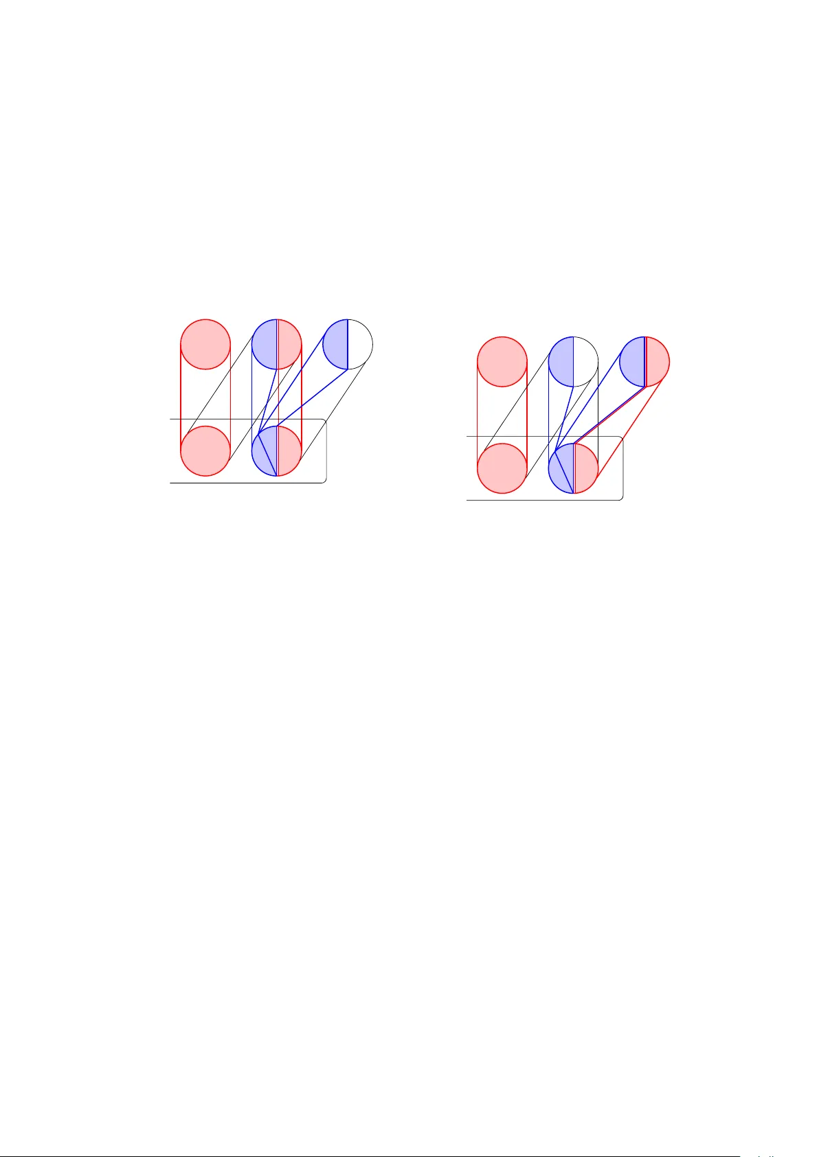
THE ASYMPTOTIC VERSION OF THE ERD ˝ OS-S ´ OS CONJECTURE AND BEYOND AKBAR D A V OODI, DIANA PIGUET, HANKA ˇ RAD A, AND NICOL ´ AS SANHUEZA-MA T AMALA Abstract. Klimo ˇ so v´ a, Piguet, and Rozhoˇ n conjectured that an y graph with mini- m um degree k / 2 and suﬃcien tly man y v ertices of degree k should con tain all trees with k edges. W e pro v e an asymptotic version of this conjecture for dense host graphs. W e obtain in teresting corollaries: the ﬁrst is an asymptotic version of the Erd˝ os–S´ os con- jecture for dense host graphs, which works without an y b ounded-degree restriction on the guest trees. Secondly , by lev eraging recent results b y P okro vsky , we can translate our results to sparse host graphs in the case of b ounded-degree guest trees. Contents 1. In tro duction 2 1.1. Rough sk etc h of the pro of of our main result 4 1.2. Organisation of the pap er 4 2. Notation 4 3. Pro of of the corollaries 5 3.1. Pro of of Corollary 1.4 5 3.2. Pro of of Corollary 1.5 6 3.3. Pro of of Corollary 1.6 8 4. Pro of of the main result 8 4.1. T ree-classes and the T ree-Coating Lemma 9 4.2. Sk ew-matc hing pairs and the Structural Prop osition 9 4.3. Reduced graph and the Embedding Lemma 9 4.4. The pro of of Theorem 1.3 10 5. Coating the T ree 12 6. Sk ew-matc hings and other matc hing structures 13 6.1. F ractional matchings 14 6.2. Sk ew-matc hings 14 6.3. Comparing matc hings 15 6.4. T runcated weigh ted graphs 17 7. F ractional structure of Gallai–Edmonds decompositions 19 7.1. F ractional matchings and c -optimal fractional matc hings 20 7.2. Reac hable v ertices 22 7.3. GE pairs 23 7.4. Separation with GE pairs 24 8. The Matc hing Lemmas 28 8.1. Basic Matc hing Lemmas 28 8.2. Adv anced Matching Lemmas 29 8.3. The pro ofs of the Basic Matching Lemmas 31 8.4. Pro of of the Improv ed Balancing Lemma 33 8.5. Pro of of the Completion Lemma 34 8.6. Pro of of the Greedy Lemmas 41 8.7. Pro of of the ( k , k / 2)-Lemma 44 9. The Structural Prop osition 51 9.1. Sk etc h of the pro of 51 9.2. Pro of of Prop osition 4.2: The fractional matching co v er case 53 1 2 A. DA V OODI, D. PIGUET, H. ˇ RADA, AND N. SANHUEZA-MA T AMALA 9.3. Pro of of Prop osition 4.2: The easy skew case 55 9.4. Pro of of Prop osition 4.2: The sk ew-matc hing co v er case 59 9.5. Pro of of Prop osition 4.2: The balanced case 69 9.6. Pro of of Prop osition 4.2: The large S R case 74 9.7. Pro of of Prop osition 4.2: The ﬂab ellum case 76 9.8. Pro of of Prop osition 4.2: The a v oiding case 79 10. Em b edding the T ree 85 10.1. Preliminaries 86 10.2. Em b edding shrubs 86 10.3. Sk etc h of the pro of 87 10.4. Pro of of Lemma 4.5: Setting the stage 87 10.5. Pro of of Lemma 4.5: Embedding the seeds 89 10.6. Pro of of Lemma 4.5: Allo cating the shrubs 90 10.7. Pro of of Lemma 4.5: Allo cating the ro ots 93 10.8. Pro of of Lemma 4.5: Finding suitable clusters 94 10.9. Pro of of Lemma 4.5: First Em bedding Phase 96 10.10. Pro of of Lemma 4.5: Second Em bedding Phase 99 11. Concluding remarks 101 11.1. Comparison with the pro of prop osed by Ajtai, Koml´ os, Simono vits, and Szemer ´ edi 101 11.2. F urther v ariations on Erd˝ os–S´ os 101 References 102 1. Introduction One of the most classical questions in graph theory is to determine the n um b er of edges in a host graph G that forces the existence of a copy of another guest graph H . T ur´ an’s theorem [ T ur41 ] giv es a complete answ er whenev er H is a clique, and the Erd˝ os– Stone–Simono vits theorem [ ES46 ; ES66 ] gives a satisfactory answer (up to lo w er order terms) for ev ery graph with chromatic n um b er at least 3. How ev er, m uc h less is kno wn for bipartite H , and even the particular case of trees remains widely op en. A seminal conjecture b y Erd˝ os and S´ os [ Erd64 ] says that graphs with av erage degree larger than k − 1 should contain all k -edge trees. Conjecture 1.1 (Erd˝ os–S´ os conjecture) . Ev ery graph G with a v erage degree d ( G ) > k − 1 con tains every tree with k edges. The conjecture has b een veriﬁed for sp eciﬁc families of trees (e.g. paths [ EG59 ], trees with diameter at most four [ McL05 ], spiders [ FHL18 ], etc. See also [ GKL16 ; Dav+18 ] for further v ariations in hypergraphs, and the survey by Stein [ Ste20 ] for more results). Besomi, Stein and Pa v ez-Sign´ e [ BPS21 ] veriﬁed the Erd˝ os–So ´ s conjecture for bounded- degree trees in dense host graphs, which then was extended to sparse host graphs by P okrovskiy [ Pok24b ]. A solution of the Erd˝ os–S´ os conjecture for all large enough trees w as announced in the early 1990s by Ajtai, Koml´ os, Simonovits and Szemer´ edi, though it has not yet b een made av ailable (a sketc h of the pro of can b e found in [ Ajt+15 ]). F or some classes of trees (suc h as stars, paths, trees with diameter at most three) even a weak er condition than that of Conjecture 1.1 on the host graph suﬃces: sp eciﬁcally , it is enough to assume that ∆( G ) ≥ k and δ ( G ) ≥ k / 2 (this can b e seen, e.g. b y follo wing the pro ofs by Erd˝ os and Gallai [ EG59 ]). This is indeed weak er, since if a graph satisﬁes d ( G ) > k − 1 then a w ell-known argument implies that G contains a subgraph G ′ with ∆( G ′ ) ≥ k and δ ( G ′ ) ≥ k / 2. Ho wev er, this new condition on the host graph is not enough to ensure the containmen t of all trees. It fails for trees of diameter four, as shown by examples of Hav et, Reed, Stein and W o o d [ Hav+20 , § 1]. In those examples, the host graphs consist either of tw o THE ASYMPTOTIC VERSION OF THE ERD ˝ OS-S ´ OS CONJECTURE AND BEYOND 3 cliques or a complete bipartite graph together with an extra univ ersal v ertex, whic h turns out to b e the unique vertex of degree at least k . In view of this situation, it is natural to think that p erhaps the following is true: if w e hav e a substantial n umber of v ertices of degree at least k in G (instead of just one), and we also hav e the condition δ ( G ) ≥ k / 2, then we should ﬁnd all k -edge trees as subgraphs of G . A conjecture along these lines was prop osed by Klimo ˇ so v´ a, Piguet, and Rozho ˇ n [ Roz19 , Conjecture 1.4]. Conjecture 1.2 (Klimo ˇ so v´ a, Piguet, Rozho ˇ n) . Ev ery n -vertex graph G with δ ( G ) ≥ k / 2 and at least n/ (2 √ k ) vertices of degree at le ast k con tains all k -edge trees. Our main result is an approximate v ersion of Conjecture 1.2 for dense graphs, i.e., with quadratically many edges. Theorem 1.3 (Main result) . F or any η , q > 0 , ther e exists an n 0 ∈ N such that for every n ≥ n 0 and al l k ≥ q n , any n -vertex gr aph G with minimal de gr e e δ ( G ) ≥ (1 + η ) k / 2 and with at le ast η n vertic es of de gr e e at le ast (1 + η ) k c ontains al l k -e dge tr e es. Theorem 1.3 implies an approximate dense version of the Erd˝ os-S´ os conjecture. Corollary 1.4. F or any η , q > 0 ther e exists an n 0 ∈ N such that for every n ≥ n 0 and al l k ≥ q n any n -vertex gr aph with aver age de gr e e mor e than (1 + η ) k c ontains any tr e e on at most k e dges as its sub gr aph. Corollary 1.4 strengthens similar results by Rozho ˇ n [ Roz19 ] and Besomi, P a vez-Sign ´ e and Stein [ BPS19 ; BPS21 ], whic h had the extra requirement that the trees T to b e found as subgraphs satisfy ∆( T ) = o ( k ). It also gives a pro of indep endent of the one prop osed by Ajtai, Koml´ os, Simonovits, and Szemer´ edi [ Ajt+15 ] in the case the host graph is dense, under the very mild strengthening that its av erage degree is required to b e sligh tly larger than k (see § 11.1 for a comparison b et w een their approach and ours). Recen tly , Reed and Stein [ Ree25 ] announced a resolution of the Erd˝ os–S´ os conjecture for the case of ‘dense trees’, i.e. that one can replace (1 + η ) k with k − 1 in Corollary 1.4 . Both of our results mentioned ab ov e work only in the setting of dense host graphs and linear-sized trees. How ever, a recent k ey structural result by P okrovskiy [ P ok24a ] pro ves that the dense case in fact encapsulates most of the diﬃculty of the general tree- em b edding problem; his result reduces problems about em b edding bounded-degree trees in host graphs (non-necessarily dense) to the case of dense host graphs. In our situation, these to ols allo w us to translate our Theorem 1.3 to the sparse setting, in the case of b ounded-degree trees. Corollary 1.5. F or ∆ ∈ N , and η > 0 , let k 0 ∈ N b e suﬃciently lar ge. Then for any k ≥ k 0 and any gr aph G with minimal de gr e e δ ( G ) ≥ (1 + η ) k / 2 and at le ast η | V ( G ) | vertic es of de gr e e at le ast (1 + η ) k c ontains as its sub gr aph any tr e e T on at most k e dges with b ounde d maximal de gr e e ∆( T ) ≤ ∆ . There is a chance that our metho ds can b e used to attac k other tree-em b edding conjectures which combine minim um and maxim um degree conditions; see § 11.2 for more discussion. As a consequence of Corollary 1.4 , we can quic kly obtain b ounds for the m ulticolour Ramsey n umbers of trees. Giv en graphs T 1 , . . . , T r , the r -c olour R amsey numb er of T 1 , . . . , T r , denoted by R r ( T 1 , . . . , T r ), is the least N so that every complete graph on N v ertices which is edge-coloured with { 1 , . . . , r } , contains a mono chromatic copy of T i in the i th colour, for some i . W e write R r ( T ) if T = T 1 = · · · = T r . Erd˝ os and Graham [ Erd81 ] conjectured that for every r ≥ 2 and every n -vertex tree T , the b ound R r ( T ) ≤ r n + O (1) should hold. This w ould follow from the v alidity of Conjecture 1.1 . The case r = 2 was pro v en by Zhao [ Zha11 ] for all large n . The following result gives an asymptotically tigh t b ound for R r ( T 1 , . . . , T r ) for arbitrary trees, generalising a result of Piguet and Stein [ PS12 ] (for tw o colours) and Klimo ˇ sov´ a, Piguet, and Rozho ˇ n [ KPR20 ] (who assumed further ‘skew’ prop erties of the trees). Also if T = T 1 = · · · = T r note that this gives an approximate version of the conjecture of Erd˝ os and Graham. 4 A. DA V OODI, D. PIGUET, H. ˇ RADA, AND N. SANHUEZA-MA T AMALA Corollary 1.6. F or r ≥ 2 and ε > 0 , ther e exists n 0 such that for any tr e es T 1 , . . . , T r with P r i =1 | V ( T i ) | ≥ n 0 , we have R r ( T 1 , . . . , T r ) ≤ (1 + ε ) P r i =1 | V ( T i ) | . 1.1. Rough sk etch of the pro of of our main result. The pro of follo ws the well- kno wn regularity metho d. First, we prepare both the host graph and the tree for em b edding (i.e., ﬁnding a cop y of the tree within the graph). W e prepare the host graph by applying Szemer ´ edi’s Regularit y Lemma, which yields the so-called r e duc e d gr aph . F or the tree, we ﬁnd a negligible set of cut v ertices that partition the tree in to smaller subtrees with sp eciﬁc prop erties. Next, in the reduced graph, we identify a suitable structure to assist in embedding the tree. This inv olves selecting tw o adjacen t clusters, each with a suﬃciently large degree relative to a structure that matc hes the shap e of the tree. One of these clusters will ha ve a total (w eighted) degree sligh tly greater than k (after re-scaling by the cluster size), a condition guaranteed by the degree-inheritance principle of the cluster graph. The second cluster will be a carefully c hosen neigh b our. These t wo adjacen t clusters will host the cut vertices of the tree. The tree-sp eciﬁc structure is designed to accommo date the small subtrees. While many previous tree-em b edding problems hav e used a simple matc hing for this structure, we hav e dev elop ed a signiﬁcantly more sophisticated ap- proac h – a skew-matching p air . This structure builds on the idea of fractional matching but assigns diﬀerent weigh ts to each end-vertex. This reﬁnemen t enables a muc h more precise replication of the global structure of the tree, oﬀering a substantial impro vemen t o ver previous methods and underscoring its k ey role in pro ving our result. Finally , we em b ed the tree using the structure established in the cluster graph during the previous phase. The embedding pro cess combines standard prop erties of regular pairs with probabilistic arguments. 1.2. Organisation of the pap er. In § 2 , we set some v ery general notation. In § 3 , w e derive from our main result ( Theorem 1.3 ) a pro of of the announced corollaries, Corollary 1.4 and Corollary 1.5 . In § 4 , we ﬁrst give some rough o verview of the pro of, and w e prov e our main result ( Theorem 1.3 ) in § 4.4 , assuming the three main tech- nical prop ositions: the T ree-Coating Lemma ( Lemma 4.1 ), the Structural Prop osition ( Prop osition 4.2 ), and the T ree-Embedding Lemma ( Lemma 4.5 ). In § 5 we prov e the T ree-Coating Lemma. The proof of the Structural Prop osition ( Prop osition 4.2 ) spans the next four sections. In § 6 we give some additional notation and deﬁnitions of the ob jects we will use in that pro of, including the key ‘skew-matc hings’. In § 7 w e inv estigate the structure of skew- matc hings in general graphs, based on known results for matc hings in graphs. In § 8 w e prov e v arious ‘building blo cks’ asso ciated with skew-matc hings that serve as lemmas in our pro of of Prop osition 4.2 (Structural Prop osition); then w e ﬁnally giv e the pro of in § 9 . Finally , in § 10 w e prov e Lemma 4.5 (T ree Embedding Lemma). W e conclude with closing remarks in § 11 . W e remark that the bulk of the length of the pap er is the pro of of the t w o main tec hnical lemmas: the pro of of the Structural Prop osition ( Prop osition 4.2 ) (which is in § 6 – § 9 ) and the pro of of the T ree-Embedding Lemma ( Lemma 4.5 ) ( § 10 ). The latter can b e read indep enden tly of the previous sections (using the deﬁnition of skew-matc hings pair as a black-box). 2. Not a tion Basic notation. W e sometimes use the hierarch y symbol ≪ , where a ≪ b informally means “ a is much smal ler than b ” , and formally translates to “there is a monotone increasing function f : (0 , 1) → (0 , 1) suc h that for an y a, b satisfying a ≤ f ( b ), the follo wing holds”. Graphs. Giv en a graph G and a subset S ⊆ V ( G ), we write G − S to refer to the graph obtained from G after removing S and any edges inciden t to S . THE ASYMPTOTIC VERSION OF THE ERD ˝ OS-S ´ OS CONJECTURE AND BEYOND 5 F or tw o disjoint subsets X and Y of V ( G ), we denote b y d ( X , Y ) the bip artite density of the pair ( X , Y ), deﬁned by d ( X , Y ) := | E ( X , Y ) | | X || Y | , in which | E ( X , Y ) | denotes the n umber of edges b etw een X and Y . F or a graph G , w e denote b y d ( G ) the aver age de gr e e of G , i.e. d ( G ) := 2 | E ( G ) | / | V ( G ) | . F or a vertex v ∈ V ( G ), let N G ( v ) denote the set of neigh b ours of v in G . W e will omit G from the notation if the graph is clear from con text. A vertex-c over of a graph G (or just c over for short) is a set C ⊆ V ( G ) such that for every edge xy ∈ E ( G ) w e ha ve { x, y } ∩ C  = ∅ . A graph H emb e ds in a graph G if there is a subgraph H ′ ⊆ G such that H ′ is isomorphic to H . Digraphs. In digr aphs every edge is orien ted, meaning that it consists of an ordered pair of v ertices, which we shall denote by a pair with an arrow on top (e.g. # » uv to mean the ordered pair ( u, v )) to diﬀerentiate w ell with the non-orien ted pairs. In the digraphs w e will use during our pro ofs w e admit cycles of length 2 (where the pairs of edges # » uv and # » v u are b oth present), but no digraph will hav e parallel edges in the same direction, and we also forbid lo ops. If every time the pair # » uv is present we also ha ve # » v u , we say that the digraph is symmetric . Given a vertex u ∈ V ( G ), the sets N + G ( u ) = { v ∈ V ( G ) : # » uv ∈ E ( G ) } and N − G ( u ) = { v ∈ V ( G ) : # » v u ∈ E ( G ) } are the outneighb ours and inneighb ours of u , resp ectiv ely . Again, we will omit G from the notation if the digraph is clear from con text. Giv en a graph G , its asso ciate d digr aph G ↔ is the digraph with the same vertex set as G and b oth # » uv and # » v u are presen t for each undirected uv ∈ E ( G ). Observe that this digraph is symmetric. Moreo ver, we use V ( G ) instead of V ( G ↔ ) and N G ( u ) instead of N + G ( u ) or N − G ( u ) when we deal with asso ciated digraphs. (It is b ecause in this case, we ha ve V ( G ) = V ( G ↔ ) and N G ( u ) = N + G ( u ) = N − G ( u ).) W eigh ted graphs and digraphs. A weighte d gr aph is a pair ( G, w ) where G is a graph and w : E ( G ) → R + is a function. W e deﬁne the weighte d de gr e e of a vertex v as deg w ( v ) := P u ∈ N ( v ) w ( v u ). W e can implicitly assume that w ( v u ) = 0 for any uv / ∈ E ( G ), so it makes sense to ev aluate w on non-edges of G . Given this assumption, w e also ha ve deg w ( v ) = P u ∈ V ( G ) w ( v u ). Given a set S ⊆ V ( G ), w e also deﬁne deg w ( v , S ) := P u ∈ S w ( v u ). Also, the minimum and maximum weighte d de gr e e are deﬁned as δ w ( G ) := min { deg w ( v ) : v ∈ V ( G ) } , and ∆ w ( G ) := max { deg w ( v ) : v ∈ V ( G ) } , resp ectively . Similarly , for v ∈ V ( G ) we deﬁne N w ( v ) := { u ∈ V ( G ) : w ( v u ) > 0 } . Similarly , we can deﬁne a w eighted digraph putting a w eight on eac h directed edge. W e will mostly consider (w eighted) digr aphs G ↔ asso ciated to w eighted graphs ( G, w ) as w ell with their w eights inherited from G , i.e. w ( # » uv ) = w ( # » v u ) = w ( uv ). Ho wev er, in general the weigh ts in digraphs do not need to b e symmetric, and w e may ha ve symmetric digraph with non-symmetric w eights 1 . Similarly as ab ov e, we can deﬁne degrees in w eighted directed graphs by deg w ( u ) := P u ∈ V ( G ) w ( # » v u ), deg w ( u, S ) := P u ∈ S w ( # » v u ), and N w ( G ) := { u ∈ V ( G ) : w ( # » v u ) > 0 } . 3. Proof of the corollaries 3.1. Pro of of Corollary 1.4 . W e pro ve that our main result ( Theorem 1.3 ) implies the asymptotic version of the Erd˝ os-S´ os Conjecture in the setting of dense graphs ( Corol- lary 1.4 ). Pr o of of Cor ol lary 1.4 . Let k = r n with r ≥ q > 0, and let G b e a graph on n v ertices with a verage degree at least (1 + η ) k . It is well-kno wn [ Die17 , Prop osition 1.2.2] that G 1 F or example, in asso ciated weigh ted digraphs G ↔ after altering its inherited weigh ts; w e may lose symmetry when using the concept of truncated weigh ted digraphs ( Deﬁnition 6.12 ). 6 A. DA V OODI, D. PIGUET, H. ˇ RADA, AND N. SANHUEZA-MA T AMALA con tains an induced subgraph H such that δ ( H ) ≥ d ( H ) / 2 ≥ d ( G ) / 2 ≥ (1 + η ) k / 2. Let m b e the num b er of vertices of H . W e clearly hav e (1 + η ) k / 2 ≤ δ ( H ) < m ≤ n . F or a giv en λ > 0, let X λ b e the set of v ertices of H whose degree in H is at least (1 + λ ) k . Then we hav e (1 + η ) k m ≤ md ( H ) = X v ∈ V ( H ) deg H ( v ) ≤ | X λ | m + ( m − | X λ | )(1 + λ ) k , whic h, by rearranging, giv es | X λ | ≥ ( η − λ ) k m m − (1 + λ ) k ≥ ( η − λ ) k . F rom now on, ﬁx the c hoice λ := η k / ( m + k ). This choice satisﬁes η ≥ λ ≥ η r / (1 + r ), and from the previous calculations w e deduce that H satisﬁes δ ( H ) > (1 + λ ) k/ 2, and has at least ( η − λ ) k = λm vertices of degree at least (1 + λ ) k . Th us, the statement follo ws b y applying Theorem 1.3 to H , with λ pla ying the role of η . ■ 3.2. Pro of of Corollary 1.5 . Now w e prov e Corollary 1.5 , whic h is a sparse version of Theorem 1.3 for b ounded-degree trees. W e shall use the following very recen t ‘hyper- stabilit y’ result of Pokro vskiy [ Pok24a , Theorem 5.2]. Theorem 3.1. F or any ∆ ≥ 1 and ε > 0 , ther e exists d > 0 such that the fol lowing holds. L et T b e a tr e e with d e dges and ∆( T ) ≤ ∆ . F or any n -vertex gr aph G having no c opies of T , it is p ossible to delete εdn e dges to get a gr aph H e ach of whose c omp onents has a vertex-c over of or der at most (2 + ε ) d . W e shall also use the following result of Piguet and Stein [ PS12 , Theorem 2], whic h is a dense approximate version of the Lo ebl–Koml´ os–S´ os conjecture. Theorem 3.2. L et η , q ≫ 1 /n . L et G b e an n -vertex gr aph G and k ≥ q n . If at le ast half of the vertic es in G have de gr e e at le ast (1 + η ) k , then G c ontains every tr e e with at most k e dges. Pr o of of Cor ol lary 1.5 . The pro of consists of several steps. First, w e apply Theorem 3.1 to obtain a subgraph with nearly the same n um b er of edges, but comp osed of a union of comp onents, eac h with a small v ertex-co ver. In the second step, we select a suitable comp onen t to work with and consider tw o cases: either the comp onen t is suﬃciently small, or it is still quite large. In the ﬁrst case, w e reﬁne the comp onen t to obtain a subgraph H 1 whic h retains similar prop erties to the original graph. Exploiting the small size of the comp onent, we reduce the problem to its dense instance and apply Theorem 1.3 (our main result) to H 1 to ﬁnd a copy of the tree. In the second case, we carefully select a small subgraph H 2 of the comp onen t that includes the entire vertex- co ver. This reduction transforms the problem in to the dense instance of the Lo ebl- Koml´ os-S´ os case, so w e can apply Theorem 3.2 to H 2 to obtain a copy of the tree. Step 1: De c omp osition via hyp erstability. Let ∆ ∈ N and η > 0 b e given. Set ε :=  η 8  4 , η ′ := η 6 2 , and let k 0 b e large enough such that it satisﬁes the requiremen t on d in Theorem 3.1 with input ∆ and ε , and ensures k 0 ≥ q n for an y n ≥ n 0 , where q = max  ε − 1 , ∆  and n 0 is the largest threshold required by Theorems 3.2 and 1.3 , so that the conditions of b oth theorems are satisﬁed. Let T b e a tree on at most k edges with ∆( T ) ≤ ∆. Assume that G do es not con tain an y copy of T , as otherwise w e are done. By Theorem 3.1 , we can erase a set of edges E ′ ⊆ E ( G ) with | E ′ | ≤ εk n so that the resulting graph H = ( V ( G ) , E ( G ) \ E ′ ) consists of comp onents C 1 , . . . , C t , eac h of which has a cov er of order at most 3 k . THE ASYMPTOTIC VERSION OF THE ERD ˝ OS-S ´ OS CONJECTURE AND BEYOND 7 Step 2: Comp onent sele ction. Let L := { v ∈ V ( G ) : deg G ( v ) ≥ (1 + η ) k } and L i = L ∩ C i . Let I − := { i ∈ [ t ] : | L i | < η 2 | C i |} and I + := [ t ] \ I − . Let L + := S i ∈ I + L i . W e hav e | L + | = | L | − | L − | ≥ η n − X i ∈ I − | L i | > η n − η 2 X i ∈ I − | C i | ≥ η 2 n  2 − P i ∈ I − | C i | n  ≥ η 2 n. W e shall discard S i ∈ I − C i and consider only H + := S i ∈ I + C i , where each comp onent con tains a substantial p ortion of its v ertices of large degree (in G ). Let B i := { v ∈ C i : deg H ( v ) < deg G ( v ) − η 8 k } . In words, B i corresp onds to those v ertices in C i whose degree dropp ed substantially when erasing the edges E ′ . W e hav e X i ∈ I + | B i | =       [ i ∈ I + B i       ≤       [ i ∈ [ t ] B i       ≤ 2 | E ′ | η k / 8 ≤ 16 εk n η k = 16 ε η n, whic h implies that X i ∈ I + | C i | ≥ X i ∈ I + | L i | = | L + | ≥ η n 2 ≥ η 2 · η 16 ε X i ∈ I + | B i | . Hence, there is an index i 0 ∈ I + suc h that | C i 0 | ≥ η 2 32 ε | B i 0 | . (1) W e select this comp onen t and show there is a cop y of T in C i 0 . Step 3: Smal l c omp onent c ase - r e duction to the dense c ase. First, assume that | C i 0 | < ( η ′ ) − 1 k . Then observe that, by ( 1 ), | B i 0 | ≤ 32 ε η 2 | C i 0 | < 32 ε η ′ η 2 k < η 4 k . Set H 1 := H [ C i 0 \ B i 0 ]. T rivially | V ( H 1 ) | ≤ | C i 0 | holds. Then, as i 0 ∈ I + , w e ha ve | L i 0 ∩ V ( H 1 ) | ≥ | L i 0 | − | B i 0 | ≥ η 2 | C i 0 | − 32 ε η 2 | C i 0 | ≥ η 4 | C i 0 | ≥ η ′ | V ( H 1 ) | . Moreo ver, for ev ery v ∈ V ( H 1 ), w e ha v e deg H 1 ( v ) ≥ deg H ( v ) − | B i 0 | ≥ deg G ( v ) − η 8 k − η 4 k . Therefore, δ ( H 1 ) ≥ (1 + η ) k / 2 − 3 η 4 k / 2 ≥ (1 + η ′ ) k / 2 and for an y v ∈ L i 0 ∩ V ( H 1 ), we obtain deg H 1 ( v ) ≥ (1 + η ) k − 3 η 8 k ≥ (1 + η ′ ) k . W e thus can apply Theorem 1.3 to H 1 (in which w e hav e at least k vertices), with η ′ pla ying the role of η , k / | V ( H 1 ) | implicitly satisfying the role of q , and k corresp onding to itself. This allows us to obtain a cop y of T in H 1 ⊆ G . Step 4: L ar ge c omp onent c ase - r e duction to the L o ebl-Koml´ os-S´ os dense c ase. W e are left to consider the case when | C i 0 | ≥ ( η ′ ) − 1 k . Let D i 0 b e the vertex-co v er of C i 0 of size at most 3 k . This means that every edge in C i 0 is incident to at least one vertex in D i 0 . No w, w e note that | L i 0 | ≥ η 2 | C i 0 | > 32 ε η 2 | C i 0 | + η 4 | C i 0 | ≥ | B i 0 | + η 4 η ′ k ≥ | B i 0 | + 3 | D i 0 | , where the ﬁrst inequality holds since i 0 ∈ I + , and the remaining inequalities follow from ( 1 ), the choices of parameters ε and η ′ , and | D i 0 | ≤ 3 k . Hence, we can c ho ose U i 0 as a subset of L i 0 \ ( D i 0 ∪ B i 0 ) with size 2 | D i 0 | . No w, w e set H 2 := H [ U i 0 ∪ D i 0 ]. Observe that as D i 0 is a v ertex-co ver and disjoin t from U i 0 , so every vertex in U i 0 has all of its neighbors in H 2 in D i 0 . F or any vertex v ∈ U i 0 ∩ V ( H 2 ), w e ha v e deg H 2 ( v ) = deg H ( v ) ≥ deg G ( v ) − η 8 k ≥ (1 + η ′ ) k . This is b ecause deg G ( v ) ≥ (1 + η ) k for v ∈ U i 0 ⊆ L i 0 , and since U i 0 ∩ B i 0 = ∅ , the v ertex v lost at most η 8 k of its degree in passing from G to H . 8 A. DA V OODI, D. PIGUET, H. ˇ RADA, AND N. SANHUEZA-MA T AMALA As ensuring a suﬃcien tly high minim um degree in H 2 is c hallenging, our strategy is to apply Theorem 3.2 instead of Theorem 1.3 to H 2 . T o apply Theorem 3.2 , we note that | V ( H 2 ) | = | U i 0 | + | D i 0 | = 3 | D i 0 | ≤ 9 k . Since | U i 0 | = 2 | D i 0 | > | V ( H 2 ) | 2 , the conditions of Theorem 3.2 are satisﬁed. Thus, we apply Theorem 3.2 to H 2 (in which w e hav e at least k vertices), with k / | V ( H 2 ) | playing the role of q , η ′ pla ying the role of η , and | V ( H 2 ) | playing the role of n . These choices ensure that the conditions of the theorem are satisﬁed, allowing us to ﬁnd a cop y of T in H 2 ⊆ G . This ﬁnishes this case, and since there are no more cases, this ﬁnishes the proof. ■ W e remark that, using the stabilit y result of Pokro vsky ( Theorem 3.1 ) in conjunction with our dense appro ximate v ersion of the Erd˝ os-S´ os conjecture ( Corollary 1.4 ), it is p os- sible to deduce an appro ximate version of the Erd˝ os-S´ os conjecture for b ounded-degree trees in sparse graphs. How ever, this w as already deduced by P okrosvky [ P ok24a , Theo- rem 1.6] from the results of Rozho ˇ n [ Roz19 ] and Besomi, Pa v ez-Sign´ e and Stein [ BPS19 ; BPS21 ] men tioned in the in tro duction. In fact, this strategy w as used to obtain an exact v ersion of the Erd˝ os-S´ os conjecture for large, b ounded-degree trees [ P ok24a , Theorem 1.16]. This strengthening additionally requires further stabilit y analysis based on ideas of Besomi, Pa vez-Sign ´ e and Stein [ BPS21 ], see [ Pok24b ] for full details. 3.3. Pro of of Corollary 1.6 . Pr o of of Cor ol lary 1.6 . W e pro ve it with 2 r ε in place of ε . Let n := P r i =1 | V ( T i ) | , whic h w e assume to b e suﬃcien tly large with resp ect to r and ε ; and let N := (1 + 2 r ε ) n . Let K N b e r -edge-coloured. By a veraging, there m ust exist i ∈ { 1 , . . . , r } suc h that the subgraph G i consisting of the i th coloured edges has av erage degree at least (1 + ε ) max {| V ( T i ) | , εn } . By Corollary 1.4 , G i m ust con tain each tree with at most max {| V ( T i ) | , εn } ≥ | E ( T i ) | edges, so in particular there is an i -coloured cop y of T i in K N , as desired. ■ 4. Proof of the main resul t This section fo cuses on pro ving Theorem 1.3 . The proof relies on the regularity metho d, which consists of three standard steps: pre-pro cessing the host graph G using Szemer ´ edi’s Regularity Lemma ( Theorem 4.3 ) which yields a so-called r e duc e d gr aph that captures the large-scale structure of G . Then, we ﬁnd a suitable structure ( Prop o- sition 4.2 ) in the reduced graph. Finally , w e use the structure in the reduced graph to em b ed the guest tree T in G ( Lemma 4.5 ). Before delving into the pro of, we pro vide some insights and outline three key state- men ts necessary for this pro of. (Readers unfamiliar with the regularit y metho d and its terminology can c heck § 4.3 for the main concepts and deﬁnitions.) W e will iden tify a sp eciﬁc structure in the reduced graph of the host graph, which w e call a skew-matching p air (see Deﬁnition 6.4 ). This structure helps in em b edding the tree. Similar to how a ‘connected matc hing’ in the reduced graph serves as a guide to embed a long path or a cycle in a host graph, a skew-matc hing pair in the reduced graph will corresp ond to a sp eciﬁc part of the host graph where there is enough space to em b ed the tree. How ever, the shap e of the sk ew-matching pair is heavily dep endent on the structure of the tree w e wan t to embed. T o understand what kind of shap e we need, we will observe that an y tree can b e broken do wn into a negligible-sized set of cut v ertices and tw o forests F A , F B that consist of tin y trees. What is most relev ant here is the colour classes (i.e. the natural bipartition) of the forests F A and F B . T rees with forests with colour classes of the same sizes are group ed in to the same tree-class T . Then the skew-matc hing pair enco des and represents some tree-class T . With this structure in mind, we can expand our initial discussion of the three main necessary lemmas for our approac h. W e hav e a host graph G and a guest tree T whic h w e need to embed into G . The ﬁrst element of the pro of is the T ree-Coating Lemma ( Lemma 4.1 ), which guarantees that T belongs to a tree-class T , according to the THE ASYMPTOTIC VERSION OF THE ERD ˝ OS-S ´ OS CONJECTURE AND BEYOND 9 partition into cut vertices and forests which we mentioned b efore. This tree-class T deﬁnes the sk ew-matching pair w e will lo ok for in the reduced graph of G . The second elemen t we need is the Structural Prop osition ( Prop osition 4.2 ), that ensures that the required skew-matc hing pair exists in the reduced graph. Finally , we need the T ree- Em b edding Lemma ( Lemma 4.5 ). This lemma states that if the reduced graph contains a sp eciﬁc skew-matc hing pair, w e can embed in the host graph G an y tree b elonging to the tree-class this pairs represents. This gives an em b edding of T into G , as desired. T o k eep this section from becoming to o complex due to hea vy notation and deﬁnitions, w e are inten tionally lea ving out the precise deﬁnitions of the skew-matc hing pair and the corresp onding tree-classes for now, treating these concepts as black-box structures. W e will provide exact deﬁnitions when needed, in § 6 and § 5 , respectively . 4.1. T ree-classes and the T ree-Coating Lemma. W e b egin by stating our T ree- Coating Lemma. This lemma ensures that any tree T b elongs to a tree-class, dep ending on the outcome of some pro cess whic h decomp oses the tree in to small parts. This decomp osition dep ends on a parameter ρ > 0 which we are free to choose. As explained ab o ve, this gives a set of cut-v ertices of negligible size and tw o forests F A and F B of tin y trees. Let a 1 , a 2 b e the size of the colour classes of F A , and b 1 , b 2 the colour classes of F B . W e then include T in the tree-class T ρ a 1 ,a 2 ,b 1 ,b 2 (see Deﬁnition 5.3 ). F or tec hnical reasons, it is not actually T which is going to b e decomp osed but instead some slightly larger sup ertree T ′ ⊃ T , which is given by the following lemma. Lemma 4.1 (T ree-Coating Lemma) . F or any 1 / 16 ≥ η ≥ ρ > 0 and any tr e e T of size | V ( T ) | ≥ 1000 /ρ , ther e ar e natur al numb ers a i , b i ≥ η | V ( T ) | for i ∈ [2] , and ther e is a tr e e T ′ ⊃ T b elonging to T ρ a 1 ,a 2 ,b 1 ,b 2 with | V ( T ′ ) | ≤ (1 + 4 η ) | V ( T ) | . The pro of of Lemma 4.1 , together with the deﬁnition of T ρ a 1 ,a 2 ,b 1 ,b 2 , are deferred to § 5 . 4.2. Sk ew-matching pairs and the Structural Prop osition. A sk ew-matching σ is a substructure of a weigh ted graph, inspired by the concept of fractional matchin g. W e ha ve a ﬁxed ‘skew’ v alue γ > 0 and for every edge uv w e attribute some non-negative w eight whic h is distributed unequally betw een u and v , in a ratio of γ . The weigh t W ( σ ) of a skew-matc hing σ represents its size, i.e. the sum of all weigh ts assigned to all edges. A ( γ A , γ B )-sk ew-matching pair ( σ A , σ B ) consists of t wo sk ew-matchings σ A and σ B , eac h with resp ectiv e skew parameters γ A and γ B . Additionally , these skew-matc hings will b e w ell-p ositioned relativ e to each other. Prop osition 4.2 (Structural Prop osition) . L et a 1 , a 2 , b 1 , b 2 ∈ N b e such that a 1 + a 2 + b 1 + b 2 = k and let ( H , w ) b e a weighte d gr aph with w : E ( H ) → (0 , 1] such that δ w ( H ) ≥ k 2 and ∆ w ( H ) ≥ k . L et γ A := a 2 a 1 and γ B := b 2 b 1 . Then H admits a ( γ A , γ B ) - skew-matching p air ( σ A , σ B ) with weights W ( σ A ) = a 1 + a 2 and W ( σ B ) = b 1 + b 2 . In § 6 , one can ﬁnd the deﬁnition of a skew-matc hing pair, as w ell as all the notions needed to prov e Proposition 4.2 . Then the pro of of Prop osition 4.2 is given in § 9 . 4.3. Reduced graph and the Embedding Lemma. As already men tioned, we use the Szemer ´ edi Regularit y Lemma [ Sze78 ] on the host graph to obtain a regular partition. The necessary deﬁnitions to work with graph regularity are as follo ws. Given a graph G and ε > 0, a pair ( X , Y ) with X , Y ⊆ V ( G ) disjoin t, is said to b e ε -r e gular , if for any sets X ′ ⊆ X and Y ′ ⊆ Y with | X ′ | ≥ ε | X | and | Y ′ | ≥ ε | Y | it holds that | d ( G [ X ′ , Y ′ ]) − d ( G [ X , Y ]) | < ε . W e say that a partition { V 0 , . . . , V t } of V ( G ) is an ε -r e gular p artition if | V 0 | ≤ ε | V ( G ) | , and for ev ery 1 ≤ i ≤ t , all but at most εt v alues of 1 ≤ j ≤ t are such that the pair ( V i , V j ) is not ε -regular. W e call an ε -regular partition e quitable if | V i | = | V j | for ev ery 1 ≤ i < j ≤ t . The follo wing version of the Regularit y Lemma follo ws b y standard arguments from its ‘degree form’ [ KS96 , Theorem 1.10]. 10 A. DA V OODI, D. PIGUET, H. ˇ RADA, AND N. SANHUEZA-MA T AMALA Theorem 4.3 (Szemer´ edi’s Regularit y Lemma) . F or every ε > 0 ther e is n 0 and M 0 such that every gr aph of size at le ast n 0 admits an ε -r e gular e quitable p artition { V 0 , V 1 , . . . , V t } with 1 /ε ≤ t ≤ M 0 . This regular partition is then captured in a weighte d r e duc e d gr aph , as deﬁned b elow. Deﬁnition 4.4 (W eighted d -reduced graph) . Given a graph G , an ε -regular equitable partition P = { V 0 , . . . , V t } of V ( G ) and d > 0, we deﬁne the d -r e duc e d gr aph Γ d ,ε as follo ws. The vertex set of Γ d ,ε is { 1 , . . . , t } , and there is an edge ij ∈ E (Γ d ,ε ) if and only if the pair ( V i , V j ) is ε -regular and d ( V i , V j ) ≥ d . The weighte d d -r e duc e d gr aph consists of Γ d ,ε endo wed with a natural w eight function w : E (Γ d ,ε ) → [0 , 1] deﬁned by w ( ij ) = d ( V i , V j ). Note that Γ d ,ε dep ends on the choice of the partition P , but since it will alw ays b e clear from con text which partition is b eing used, w e omit it from the notation. W e shall apply the Structural Proposition ( Prop osition 4.2 ) in the weigh ted d -reduced graph Γ d ,ε to obtain a sk ew-matching pair there. That is precisely the input which the next lemma requires, and it provides an embedding of a tree in the original host graph. Lemma 4.5 (T ree Embedding Lemma) . F or any η , d , q > 0 , and t ∈ N , ther e ar e ε = ε ( η , d , q ) , ρ = ρ ( η , d , q , t ) > 0 and n 0 = n 0 ( η , d , q , t ) ∈ N such that for n ≥ n 0 the fol lowing holds. Supp ose G is an n -vertex gr aph, and P = { V 0 , V 1 , . . . , V N } is an ε -r e gular e quitable p artition of G with N ≤ t . Supp ose k ≥ q n and that we have natur al numb ers a 1 , b 1 , a 2 , b 2 ≥ η k such that k = a 1 + a 2 + b 1 + b 2 . Supp ose the weighte d d -r e duc e d gr aph Γ d ,ε c orr esp onding to G admits a ( a 2 /a 1 , b 2 /b 1 ) - skew-matching p air ( σ A , σ B ) , with weights W ( σ A ) ≥ (1 + η )( a 1 + a 2 ) N /n and W ( σ B ) ≥ (1 + η )( b 1 + b 2 ) N /n . Then G c ontains any tr e e T ∈ T ρ a 1 ,a 2 ,b 1 ,b 2 . Lemma 4.5 is prov en in § 10 . 4.4. The pro of of Theorem 1.3 . Now, w e give the pro of of Theorem 1.3 , assuming the v alidit y of the main statemen ts in tro duced b efore ( Lemma 4.1 , Prop osition 4.2 , Lemma 4.5 ). Pr o of of The or em 1.3 . The pro of splits naturally into four steps. Step 1: Setting up the p ar ameters. Supp ose we are given input parameters η > 0 for the approximation factor, and q > 0 for the ratio of the size of the tree s with resp ect to the size of the host graph. W e may assume that q , η ≪ 1, or we just replace them with smaller v alues. W e set the follo wing parameters to satisfy 0 < 1 /n 0 ≪ ρ ≪ 1 / M 0 ≪ ε ≪ d ≪ η , q ≪ 1 , (2) as follows. W e set d := η q 100 , ε := min { d 2 , ε ′ } , where ε ′ is the output of the T ree Embedding Lemma ( Lemma 4.5 ) giv en the input η / 40, d , and q pla ying the roles of η , d , and q re- sp ectiv ely . Let M 0 , n ′ 0 b e the outputs of the Szemer ´ edi Regularit y Lemma ( Theorem 4.3 ) with input ε . Let ρ, n ′′ 0 b e the output of the T ree Embedding Lemma ( Lemma 4.5 ) with input η / 40 , d , q , M 0 in place of η , d , q , t . Finally , let n 0 = max { n ′ 0 , n ′′ 0 , 1000 /ρ } . Step 2: Pr o c essing the tr e e. W e apply the T ree-Coating Lemma ( Lemma 4.1 ) with input η / 12, ρ , and T , playing the roles of η , ρ , and T . W e obtain T ′ ∈ T ρ a 1 ,a 2 ,b 1 ,b 2 with a i , b i ≥ η k 12 ≥ η 20 | V ( T ′ ) | and | V ( T ′ ) | ≤ (1 + η 3 ) k . Recall that, by assumption, the host graph G satisﬁes δ ( G ) ≥ (1 + η ) k 2 ≥ (1 + η 20 ) | V ( T ′ ) | 2 and that at least η n 20 v ertices of G ha ve degree at least (1 + η ) k ≥ (1 + η 20 ) | V ( T ′ ) | . Step 3: Pr ep a ring the host gr aph. W e apply the Szemer ´ edi Regularity Lemma ( Theo- rem 4.3 ) on G with parameter ε . This application yields an ε -regular equitable partition THE ASYMPTOTIC VERSION OF THE ERD ˝ OS-S ´ OS CONJECTURE AND BEYOND 11 { V 0 , V 1 , . . . , V t } , with 1 /ε ≤ t ≤ M 0 . Giv en this partition, we deﬁne the weigh ted d - reduced graph Γ d ,ε endo wed with the weigh t function w : E (Γ d ,ε ) → [0 , 1], deﬁned by w ( ij ) := d ( V i , V j ). Recall that by the deﬁnition of Γ d ,ε , if ( V i , V j ) is not an ε -regular pair, or if d ( V i , V j ) < d , then ij ∈ E (Γ d ,ε ). F rom no w on, let r = k /n . Standard calculations sho w that Γ d ,ε inherits minimum and maximum degree conditions from G . Concretely , w e claim that (Γ d ,ε , w ) satisﬁes δ w (Γ d ,ε ) ≥ (1 + η 40 ) rt 2 and ∆ w (Γ d ,ε ) ≥ (1 + η 40 ) r t . W e give those arguments for complete- ness. Indeed, for i ∈ V (Γ d ,ε ) w e ha v e deg w ( i ) = X j ∈ N Γ d ,ε ( i ) w ( ij ) = X j ∈ N Γ d ,ε ( i ) d ( V i , V j ) ≥   X j ∈ [ t ] \{ i } d ( V i , V j )   − ( ε + d ) t =   X j ∈ [ t ] \{ i } X v ∈ V i deg G ( v , V j ) | V i | 2   − ( ε + d ) t ≥ X v ∈ V i deg G ( v ) − | V i | | V i | 2 − ( ε + d ) t ≥ δ ( G ) | V i | − 1 − ( ε + d ) t ≥ (1 + η ) k / 2 | V i | − (2 ε + d ) t = (1 + η ) r n/ 2 | V i | − (2 ε + d ) t ≥ (1 + η ) r t 2 − (2 ε + d ) t ≥  1 + η 40  r t 2 , where we used | V i | ≤ n/t in the second to last inequality , and r ≥ q and the choice of d , ε in the last inequality . T o calculate ∆ w (Γ d ,ε ), denote b y L the set of v ∈ V ( G ) such that deg w ( v ) ≥ (1 + η ) k = (1 + η ) r n . By the pigeonhole principle, there is an index i ∈ [ t ] with | V i ∩ L | ≥ η n − εn t ≥ η (1 − ε ) n/t ≥ η (1 − ε ) | V i | > ε | V i | . Then deg w ( i ) = X j ∈ N Γ d ,ε ( i ) w ( ij ) = X j ∈ N Γ d ,ε ( i ) d ( V i , V j ) ≥   X j ∈ [ t ] \{ i } d ( V i , V j )   − ( ε + d ) t ≥   X j ∈ [ t ] \{ i } d ( V i ∩ L, V j ) − ε   − ( ε + d ) t ≥   X v ∈ V i ∩ L deg G ( v ) − | V i | | V i ∩ L || V i |   − (2 ε + d ) t ≥   X v ∈ V i ∩ L (1 + η ) k | V i ∩ L || V i |   − 1 − (2 ε + d ) t ≥ (1 + η ) k | V i | − (3 ε + d ) t = (1 + η ) r n | V i | − (3 ε + d ) t ≥ (1 + η ) r t − (3 ε + d ) t ≥  1 + η 40  r t, where we used | V i | ≤ n/t in the second to last inequality , and r ≥ q and the choice of d , ε in the last inequality . These estimates on δ w (Γ d ,ε ) and ∆ w (Γ d ,ε ) allo w us to apply the Structural Prop osition ( Prop osition 4.2 ) with (Γ d ,ε , w ), (1 + η 40 ) r t , (1 + η 40 ) a i t/n and (1 + η 40 ) b i t/n pla ying the roles of ( H, w ), k and a i , b i , for i ∈ [2], resp ectively . W e obtain an ( a 2 a 1 , b 2 b 1 )-sk ew-matching ( σ A , σ B ) with W ( σ A ) = (1 + η 40 )( a 1 + a 2 ) t/n and W ( σ B ) = (1 + η 40 )( b 1 + b 2 ) t/n . Step 4: Emb e dding the tr e e. Having found the sk ew-matching pair in the reduced graph, w e ﬁnalise by applying the T ree Em b edding Lemma ( Lemma 4.5 ). First, w e note that min { a 1 , a 2 } ≥ η 20 | V ( T ′ ) | ≥ η 40  (1 + η 40 ) | V ( T ′ ) |  and similarly for b 1 , b 2 , we hav e that min { b 1 , b 2 } ≥ η 40 ((1 + η 40 ) | V ( T ′ ) | ). Th us, we can apply the T ree Embedding Lemma 12 A. DA V OODI, D. PIGUET, H. ˇ RADA, AND N. SANHUEZA-MA T AMALA ( Lemma 4.5 ) with t and η / 40, pla ying the roles of N and η , resp ectively . W e obtain that G con tains any tree in T ρ a 1 ,b 1 ,a 2 ,b 2 , so in particular T ′ ⊆ G . Since T ⊆ T ′ , this pro ves Theorem 1.3 . ■ 5. Coa ting the Tree T o prepare the embedding, we will ﬁrst partition the trees in to suitably small parts. W e will use the following handy concept from Hladk ´ y, Koml´ os, Piguet, Simonovits, Stein, and Szemer ´ edi [ Hla+17 , Deﬁnition 3.3]. It gives a partition of a tree into smaller trees that also satisfy several additional useful prop erties. If T is a tree ro oted at r , and e T ⊆ T is a subtree with r / ∈ V ( e T ), the se e d of e T is the unique vertex x ∈ V ( T ) \ V ( e T ) which is farthest from r and also b elongs to ev ery ( r , v )-path in T , for ev ery v ∈ V ( e T ). W e emphasize that the seed of e T is not con tained in V ( e T ), and that e T do es not necessarily con tain all descendants of its seed. Deﬁnition 5.1 ( ℓ -ﬁne partition) . Let T b e a tree on k vertices ro oted at a v ertex r . An ℓ -ﬁne p artition of T is a quadruple ( W A , W B , F A , F B ), where W A , W B ⊆ V ( T ) and F A , F B are families of subtrees of T suc h that (A1) the three sets W A , W B , and { V ( T ∗ ) } T ∗ ∈F A ∪F B partition V ( T ) (in particular, the trees in F A ∪ F B are pairwise vertex-disjoin t), (A2) r ∈ W A ∪ W B , (A3) max {| W A | , | W B |} ≤ 336 k /ℓ , (A4) for w 1 , w 2 ∈ W A ∪ W B , the distance b etw een w 1 and w 2 in T is o dd if and only if one of them lies in W A and the other one in W B , (A5) | V ( T ∗ ) | ≤ ℓ for every T ∗ ∈ F A ∪ F B , (A6) V ( T ∗ ) ∩ N ( W B ) = ∅ for every T ∗ ∈ F A , and V ( T ∗ ) ∩ N ( W A ) = ∅ for every T ∗ ∈ F B ; (A7) each tree of F A ∪ F B has its seeds in W A ∪ W B , (A8) | N ( V ( T ∗ )) ∩ ( W A ∪ W B ) | ≤ 2 for each T ∗ ∈ F A ∪ F B , (A9) if N ( V ( T ∗ )) ∩ ( W A ∪ W B ) contains tw o distinct v ertices w 1 , w 2 for some T ∗ ∈ F A ∪ F B , then dist T ( w 1 , w 2 ) ≥ 6. The trees T ∗ ∈ F A ∪ F B will b e called shrubs . W e remark that ℓ -ﬁne partitions can be deﬁned diﬀerently so they satisfy even more prop erties, but w e are only citing those we need. See Figure 1 for a visual representation of a tree together with an ℓ -ﬁne partition. The next lemma [ Hla+17 , Lemma 3.5] says that an y tree has an ℓ -ﬁne partition. Lemma 5.2. L et T b e a tr e e on k vertic es r o ote d at r , and let 1 ≤ ℓ ≤ k . Then T has an ℓ -ﬁne p artition. Deﬁnition 5.3 (T ree-class T ρ a 1 ,a 2 ,b 1 ,b 2 ) . W e denote by T ρ a 1 ,a 2 ,b 1 ,b 2 the set of trees T , suc h that there is a ( ρ | V ( T ) | )-ﬁne partition ( W A , W B , F A , F B ) of T such that | V i ( F A ) | = a i , | V i ( F B ) | = b i , for i ∈ { 1 , 2 } , where V 1 ( F A ) (resp. V 2 ( F A )) is the set of vertices of F A that are at odd (resp. even) distance from W A , and V i ( F B ) are deﬁned analogously with resp ect to W B . As mentioned earlier, for tec hnical reasons we shall work with a tree T ′ ⊃ T which is sligh tly larger than T , but that b elongs to the class T ρ a 1 ,a 2 ,b 1 ,b 2 for some suitable v alues of a 1 , a 2 , b 1 , b 2 . In our case ‘suitable’ will mean that none of these v alues are very small; this fact will b e useful during the embedding phase later. The T ree-Coating Lemma ( Lemma 4.1 ) describ es precisely the pro cess of ﬁnding this sup ertree T ′ . W e no w hav e the to ols and vocabulary to prov e it. W e restate the statement for the conv enience of the reader. THE ASYMPTOTIC VERSION OF THE ERD ˝ OS-S ´ OS CONJECTURE AND BEYOND 13 r ∈ W A T ∗ 2 ∈ F A ∈ W A W B ∋ T ∗ 5 ∈ F B T ∗ 4 ∈ F A T ∗ 1 ∈ F A W B ∋ W A ∋ T ∗ 3 ∈ F A Figure 1. A schematic view of an ℓ -ﬁne partition of a tree with 45 vertices ro oted at r in to W A , W B , F A , F B , satisfying (A1) – (A9) . Lemma 4.1 (T ree-Coating Lemma) . F or any 1 / 16 ≥ η ≥ ρ > 0 and any tr e e T of size | V ( T ) | ≥ 1000 /ρ , ther e ar e natur al numb ers a i , b i ≥ η | V ( T ) | for i ∈ [2] , and ther e is a tr e e T ′ ⊃ T b elonging to T ρ a 1 ,a 2 ,b 1 ,b 2 with | V ( T ′ ) | ≤ (1 + 4 η ) | V ( T ) | . Pr o of of Lemma 4.1 . Pick any vertex r ∈ V ( T ) as the ro ot of T and apply Lemma 5.2 with input T , | V ( T ) | , r , and ρ | V ( T ) | , playing the roles of T , k , r and ℓ to obtain a ρ | V ( T ) | -ﬁne partition of T . First assume that b oth W A and W B are non-empty . Pick a v ertex x A ∈ W A and a vertex x B ∈ W B and attach η | V ( T ) | paths of length 2 to each of the t w o vertices x A and x B . This adds η | V ( T ) | v ertices to F L ∩ V i ( T ) for L ∈ { A, B } and i ∈ [2], where V i ( T ) , i ∈ [2] are the tw o colour classes of T , and increases the size of the tree b y 4 η | V ( T ) | . As 2 ≤ ρ | V ( T ) | , all the newly formed shrubs in F A ∪ F B ha ve size at most ρ | V ( T ′ ) | and th us, the newly obtained tree T ′ b elongs to the class T ρ a 1 ,a 2 ,b 1 ,b 2 , for suitable a i and b i , for i ∈ [2]. If (w.l.o.g.) W A = ∅ , b y Deﬁnition 5.1(A6) , we hav e that F A = ∅ . By (A3) , w e hav e | W B | ≤ 336 /ρ ≤ | V ( T ) | / 2, and therefore |F B ∩ V i ( T ) | ≥ | V ( T ) | / 4 ≥ 4 η | V ( T ) | , for some i ∈ [2]. Add a v ertex x A to W A , connecting it to an y vertex in W B , and as previously attac h η | V ( T ) | paths of length 2 to x A . F or the other side, if the vertices in F B at o dd distance to W B are less than η | V ( T ) | , then place a star with 2 η | V ( T ) | − 1 leav es centred on an arbitrary vertex x B ∈ W B . Otherwise attach η | V ( T ) | − 2 paths of length 2 to some vertex x B ∈ W B and a star with 2 lea ves and connect the centre to x B as well. In this w ay , w e ensure (as 3 ≤ ρ | V ( T ) | ) that the newly created tree b elongs to T ρ a 1 ,a 2 ,b 1 ,b 2 for suitable a i , b i ≥ η | V ( T ) | , i ∈ [2], and that w e hav e increased the tree by exactly 4 η | V ( T ) | v ertices. ■ 6. Skew-ma tchings and other ma tching structures In the next four sections, we pro ve the Structural Prop osition ( Prop osition 4.2 ). In this section, we will introduce the basic deﬁnitions that will allo w us to describ e the structure we will seek in the reduced graph. The basic building blo ck of our argumen t is a “sk ew” orien ted fractional matching, deﬁned in Section 6.2 . Its deﬁnition is inspired by the standard fractional matching, whic h (w e recall) is a w eight function ov er the edges of a graph such that the sum of weigh ts o ver the edges incident to any given v ertex is at most one ( Deﬁnition 6.1 ). As we shall see, a skew-matc hing satisﬁes a similar prop erty , but instead is a w eight function deﬁned o ver oriente d edges of the graph, whic h allo ws us to distribute the w eigh t in every edge in an un balanced w a y . W e remark that essentially equiv alent concepts w ere used b efore (e.g. [ Bal+18 , § 2.4]) in th e con text of graph tilings. 14 A. DA V OODI, D. PIGUET, H. ˇ RADA, AND N. SANHUEZA-MA T AMALA After in tro ducing the main deﬁnitions in § 6.1 and § 6.2 , we introduce many extra auxiliary concepts. In § 6.3 w e in tro duce notation to compare diﬀerent fractional match- ings and sk ew-matchings; and in § 6.4 we introduce the auxiliary notion of the trunc ate d weighte d gr aph . 6.1. F ractional matc hings. The following standard deﬁnition generalises the notion of matc hings to a fractional setting. Deﬁnition 6.1 (F ractional matc hing) . A fr actional matching is a weigh t function µ : E ( G ) → [0 , 1] such that for any vertex v ∈ V ( G ), we hav e P u ∈ N ( v ) µ ( uv ) ≤ 1. W e shall abuse notation here and use the sign µ on vertices as w ell and we call µ ( v ) := X u ∈ N ( v ) µ ( uv ) the weight of µ on v . The weight of a fractional matching µ is W ( µ ) := X e ∈ E ( G ) µ ( e ) . W e sa y that tw o fractional matchings µ ′ and µ ′′ are disjoint if µ ′ ( x ) + µ ′′ ( x ) ≤ 1 for all x ∈ V ( G ). W e denote by V ( µ ) the set of v ertices v ∈ V ( G ) suc h that µ ( v ) > 0. 6.2. Sk ew-matchings. No w we present the deﬁnition of skew-matc hings. Note that, according to our conv ention on G ↔ , b oth edges # » uv and # » v u are present in the follo wing deﬁnition. Deﬁnition 6.2 ( γ -skew orien ted fractional matching) . Let G b e a graph, G ↔ its as- so ciated digraph, and γ ≥ 0. A γ -skew oriente d fr actional matching (or just γ -skew- matching ) is a function σ : E ( G ↔ ) → [0 , 1] such that for any vertex u ∈ V ( G ), X v ∈ N ( u )  1 1 + γ σ ( # » uv ) + γ 1 + γ σ ( # » v u )  ≤ 1 . As explained b efore, γ -skew-matc hings can b e understo o d as fractional matc hings ( Deﬁnition 6.1 ) in graphs where the w eigh t of the edge is distributed in an unbalanced w ay , meaning that one end of the edge gets γ times the w eigh t of the other end, and the direction of this imbalance is given by the direction of the edge in the digraph G ↔ . With a slight abuse of notation, given a γ -skew-matc hing σ w e shall use the symbol σ on vertices as well. W e deﬁne σ ( u ) := σ 1 ( u ) + σ 2 ( u ) , where σ 1 ( u ) := 1 1 + γ X v ∈ N ( u ) σ ( # » uv ) and σ 2 ( u ) := γ 1 + γ X v ∈ N ( u ) σ ( # » v u ) . No w we deﬁne t w o crucial concepts associated with a γ -skew-matc hing σ . The anchor of σ , denoted by A ( σ ), is the set A ( σ ) := { u ∈ V ( G ) : σ 1 ( u ) > 0 } . The weight of σ is W ( σ ) := X e ∈ E ( G ↔ ) σ ( e ) . F or our pro of, we will usually need to w ork with several skew-matc hings, p ossibly with diﬀerent v alues of γ . If σ, σ ′ are γ -skew and γ ′ -sk ew-matchings resp ectively , we sa y σ, σ ′ are disjoint if, for ev ery u ∈ V ( G ), σ ( u ) + σ ′ ( u ) ≤ 1 . THE ASYMPTOTIC VERSION OF THE ERD ˝ OS-S ´ OS CONJECTURE AND BEYOND 15 In what follows, w e often w ork with a w eighted graph ( G, w ) and its asso ciated digraph G ↔ and we do not alwa ys explicitly distinguish b etw een G and G ↔ , as they are in one-to-one corresp ondence. The follo wing deﬁnition is key: it essentially sa ys that a sk ew-matching σ do es not place to o muc h w eight in the neighbourho o d of a vertex u , meaning that it resp ects the w eight dictated by some edge weigh ting w . This will allow us to embed trees using the space, allo wed by σ , that is also joined correctly with u . Deﬁnition 6.3 (Fitting in the w -neighbourho o d) . Let ( G, w ) b e a weigh ted digraph, γ ≥ 0, and u ∈ V ( G ). Given a γ -skew orien ted fractional matc hing σ , we sa y that its anc hor ﬁt s in the w -neighb ourho o d of u if σ 1 ( v ) ≤ w ( # » uv ), for every v ∈ V ( G ). Note that, in particular, if A ( σ ) ﬁts in the w -neighbourho o d of u , then A ( σ ) ⊆ N w ( u ). The follo wing deﬁnition is also key . It corresp onds to t wo skew-matc hings, with diﬀeren t skews, which are disjoin t from each other and they ﬁt in the neigh b orho o ds of tw o v ertices forming an edge cd . This will b e the structure w e desire in the reduced graph. Referencing the ℓ -ﬁne partitions of a tree T discussed b efore: the (few) v ertices of the sets W A , W B will b e mapp ed to the clusters corresp onding to cd , while the shrubs in F A , F B will b e mapp ed in the space ensured b y σ A , σ B , resp ectively . Deﬁnition 6.4 (Edge-anc hored sk ew-matching pair) . Let ( G, w ) be a weigh ted digraph, and γ A , γ B ≥ 0. A ( γ A , γ B ) -skew-matching p air anchor e d in # » cd ∈ E ( G ) is a pair ( σ A , σ B ) suc h that (B1) σ A and σ B are disjoin t, (B2) σ A is a γ A -sk ew-matching, whose anc hor ﬁts in the w -neighbourho o d of c , (B3) σ B is a γ B -sk ew-matching, whose anc hor ﬁts in the w -neighbourho o d of d , and (B4) for every x ∈ N ( c ) ∩ N ( d ), we hav e max { w ( # » cx ) , w ( # » dx ) } ≥ σ 1 A ( x ) + σ 1 B ( x ) . Observ e that there is no weigh t requirement on # » cd . W e say that a w eighted (unoriented) graph ( G, w ) admits a ( γ A , γ B )-sk ew-matching pair ( σ A , σ B ), if ( σ A , σ B ) is deﬁned on its asso ciated w eighted digraph G ↔ and is an- c hored in some edge # » cd ∈ E ( G ↔ ), and w ( cd ) > 0. Remark 6.5. W e can express (B4) equiv alently by saying that there is a partition { X c , X d } of N ( c ) ∩ N ( d ) suc h that for every x ∈ X c , w e hav e w ( # » cx ) ≥ σ 1 A ( x ) + σ 1 B ( x ), and for every x ∈ X d , w e ha v e w ( # » dx ) ≥ σ 1 A ( x ) + σ 1 B ( x ). W e say that a vertex v ∈ V ( G ) is c over e d by a fractional matching σ (or a sk ew orien ted fractional matching) if σ ( v ) = 1. Analogously , w e say that a set U is c over e d , if eac h v ertex v ∈ U is cov ered. Moreov er, we deﬁne V ( σ ) := { v ∈ V ( G ) : σ ( v ) > 0 } . The v alue deg w ( u, σ ) = X v ∈ V ( G ) min { σ ( v ) , w ( # » uv ) } is called the satur ation of N ( u ) b y σ . W e say that σ satur ates N ( u ) ∩ U for some U ⊆ V ( G ), if for every v ertex v ∈ U , we hav e that σ ( v ) ≥ w ( # » uv ). If U = V ( G ), we simply say that σ satur ates the neighbourho o d of u (or satur ates N ( u ) for short). If this happ ens, then deg w ( u ) = deg w ( u, σ ). 6.3. Comparing matc hings. Now w e deﬁne a few relations betw een fractional matc h- ings and skew-matc hings, whic h will allow us to compare them to each other. Notice that b oth edges # » xy and # » y x are often used. W e b egin b y comparing fractional matchings b etw een them. W e write µ ≤ µ ′ for tw o fractional matc hings µ and µ ′ , whenev er µ ( xy ) ≤ µ ′ ( xy ) for ev ery xy ∈ E ( G ). Moreov er, µ = µ ′ if and only if µ ( xy ) = µ ′ ( xy ) for every xy ∈ E ( G ). 16 A. DA V OODI, D. PIGUET, H. ˇ RADA, AND N. SANHUEZA-MA T AMALA Similarly , w e can compare skew-matc hings betw een them, even if they diﬀer in their sk ews. A γ ′ -sk ew-matching σ ′ is a skew sub-matching of a γ -skew matching σ , if for ev ery # » uv ∈ E ( G ↔ ), we hav e σ ′ ( # » uv ) 1+ γ ′ ≤ σ ( # » uv ) 1+ γ and γ ′ 1+ γ ′ σ ′ ( # » uv ) ≤ γ 1+ γ σ ( # » uv ). This is denoted b y σ ′ ≤ σ . In the next deﬁnition we in tro duce the language and notation to compare fractional matc hings with skew-matc hings, and vice versa. Deﬁnition 6.6 ( ⪯ , ⊴ ) . Let G be a graph with associated digraph G ↔ , let σ b e a γ -skew orien ted fractional matching in G ↔ , and let µ b e a fractional matching in G . W e write µ ⪯ σ if for every # » xy ∈ E ( G ↔ ) with µ ( xy ) > 0, we hav e µ ( xy ) ≤ 1 1 + γ σ ( # » xy ) + γ 1 + γ σ ( # » y x ) . Similarly , we write σ ⊴ µ if for ev ery # » xy ∈ E ( G ↔ ) with σ ( # » xy ) + σ ( # » y x ) > 0, we hav e σ ( # » xy ) + γ σ ( # » y x ) 1 + γ ≤ µ ( xy ) . Remark 6.7. W e emphasize that in b oth deﬁnitions, that of µ ⪯ σ and σ ⊴ µ , w e require the inequality to hold for each oriented edge in G ↔ , which means that for eac h (unorien ted) edge xy ∈ E ( G ) we need to verify the inequalit y b oth for # » xy and # » y x . F or instance, in the deﬁnition of µ ⪯ σ we need µ ( xy ) ≤ 1 1 + γ σ ( # » y x ) + γ 1 + γ σ ( # » xy ) to hold as well; and in the deﬁnition of σ ⊴ µ we also need that σ ( # » y x ) + γ σ ( # » xy ) 1 + γ ≤ µ ( xy ) . W e also in tro duce notation to compare multiple skew-matc hings with a fractional matc hing. Let σ i b e a γ i -sk ew-matching for every i ∈ [ k ]. W e write P k i =1 σ i ⊴ µ if for ev ery # » xy ∈ E ( G ↔ ) with P k i =1  σ i ( # » xy ) + σ i ( # » y x )  > 0, w e hav e k X i =1 σ i ( # » xy ) + γ i σ i ( # » y x ) 1 + γ i ≤ µ ( xy ) . Remark 6.8. In the last deﬁnition, w e compute a sum of sk ew-matchings with diﬀeren t sk ews. This sum do es not deﬁne a new skew-matc hing. W e only compare the weigh t of these s k ew-matchings on every oriented edge with the weigh t of the fractional matc hing µ on the corresp onding unoriented edge (and w e do it for b oth p ossible orientations). In this wa y w e inv estigate if all these skew-matc hings together “ﬁt” in a fractional matc hing µ . In other words, if P k i =1 σ i ⊴ µ , w e hav e P k i =1 σ i ( u ) ≤ µ ( u ) ≤ 1 for all u ∈ V ( G ). Observ ation 6.9. Let G b e a graph, G ↔ b e its asso ciated digraph, µ, b µ b e fractional matc hings in G and σ , b σ b e skew fractional matchings in G ↔ . All the v alues µ ( uv ) , σ ( # » uv ) , µ ( u ) , b µ ( u ) are non-negativ e real n um b ers. Therefore, ex- pressions suc h as µ ( uv ) ≤ σ ( # » uv ), µ ( u ) ≤ b µ ( u ), σ ( # » uv ) + µ ( uv ) are well-deﬁned. W e can also gather some straigh tforward observ ations and consequences of our pre- vious deﬁnitions, that will allow us to work more mec hanically with diﬀerent ob jects. (i) Having µ ( u ) ≤ b µ ( u ) for ev ery u ∈ V ( G ) do es not imply that µ ≤ b µ . (ii) Similarly , having σ ⊴ µ do es not imply that σ ( # » uv ) ≤ µ ( uv ) for ev ery uv . (iii) On the other hand, ha ving σ ⊴ µ implies that σ ( u ) ≤ µ ( u ) for every u ∈ V ( G ). (iv) If µ ⪯ σ and σ ⊴ b µ , then µ ≤ b µ . (v) Having σ ⊴ µ and µ ⪯ b σ do es not imply that σ ≤ b σ . (vi) If σ ⊴ µ and W ( σ ) = 2 W ( µ ), then σ ( u ) = µ ( u ) for every u ∈ V ( G ). Note that, in general, we hav e σ ( u )  = P v ∈ N ( u ) σ ( # » uv ) + σ ( # » v u ). THE ASYMPTOTIC VERSION OF THE ERD ˝ OS-S ´ OS CONJECTURE AND BEYOND 17 While fractional matc hings are deﬁned on a non-orien ted graph G and sk ew-matc hings are deﬁned on G ↔ , we can easily obtain a 1-sk ew-matching σ from a fractional match- ing µ . This can be done, for instance, b y choosing an orientation for each edge xy ∈ E ( G ) and setting σ ( # » xy ) = 2 µ ( xy ) and σ ( # » y x ) = 0. W e observe, how ever, that the deﬁnition of “w eight” in both cases diﬀers, b ecause then W ( σ ) = X # » xy ∈ E ( G ↔ ) σ ( # » xy ) = X xy ∈ E ( G ) (2 µ ( xy ) + 0) = 2 W ( µ ) . There are many diﬀeren t 1-skew-matc hings σ that we can deﬁne using a fractional matc hing µ . F or example σ ( # » xy ) = σ ( # » y x ) = µ ( xy ) is also a p ossibilit y . In this c ase, w e again obtain that W ( σ ) = 2 W ( µ ). Con versely , w e can obtain a fractional matc hing µ from a 1-sk ew-matching σ just by “forgetting” the orientation of the edges. Then, w e get W ( µ ) = X xy ∈ E ( G ) µ ( xy ) = X xy ∈ E ( G ) σ ( # » xy ) + σ ( # » y x ) 2 = W ( σ ) 2 . The next lemma encapsulates the ab ov e discussion for future reference. Lemma 6.10. L et G b e a gr aph and G ↔ its asso ciate d digr aph. L et σ b e a 1 -skew- matching in G ↔ . Then G has a fr actional matching µ such that (i) W ( µ ) = 1 2 W ( σ ) , (ii) for al l x ∈ V ( G ) , σ ( x ) = µ ( x ) , and (iii) if σ ′ is a γ -skew-matching in G ↔ such that σ ≤ σ ′ , then µ ⪯ σ ′ . In the following deﬁnition, we extend the concept of c overing and satur ation from fractional matchings or sk ew-matchings, to sum of skew-matc hings, or sum of a fractional matc hing and skew-matc hings. This is done in a natural wa y: the notions of cov ering and saturation refer to the weigh ts that the given ob jects induce on the vertices and do not dep end on the type of ob ject. Deﬁnition 6.11 (Saturation, Co vering) . Let ( G, w ) be a w eighted graph, ( G ↔ , w ) its as- so ciated w eighted digraph, ν 1 , ν 2 represen t fractional matc hings and/or skew-matc hings 2 (including the option of everywhere 0-v alued functions), and u ∈ V ( G ). Then the v alue deg w ( u, ν 1 + ν 2 ) := X v ∈ N w ( u ) min { ν 1 ( v ) + ν 2 ( v ) , w ( # » uv ) } is called the satur ation of N w ( u ) by ν 1 + ν 2 . W e say that ν 1 + ν 2 satur ates the neigh- b ourho o d of u (or satur ates N w ( u ) for short) if deg w ( u ) equals deg w ( u, ν 1 + ν 2 ). Analogously , ν 1 + ν 2 satur ates N w ( u ) ∩ U , for some U ⊆ V ( G ), if for every vertex v ∈ N w ( u ) ∩ U we ha ve ν 1 ( v ) + ν 2 ( v ) ≥ w ( # » uv ). W e say that ν 1 + ν 2 c overs a vertex v ∈ V ( G ) if ν 1 ( v ) + ν 2 ( v ) = 1. W e say that it cov ers a set S ⊆ V ( G ), if it co vers ev ery v ertex v ∈ S . 6.4. T runcated w eighted graphs. Now w e shall deﬁne another imp ortant concept used in our pro ofs, that of a trunc ate d weighte d gr aph . T o motiv ate this deﬁnition, consider the following scenario. Supp ose we need to ﬁnd a fractional matching in a w eighted graph ( G, w ) of suﬃcien tly large w eight, but so far we hav e only found a fractional matching µ of insuﬃcient weigh t. In our settings, we alw ays need to make sure our fractional ob jects (matchings or sk ew-matchings) ‘ﬁt’ in the w -neighbourho o d of a giv en vertex, sa y c . Th us, if we wan t to build another matching ¯ µ , disjoint from µ , and we wan t to consider the sum µ + ¯ µ , we need to k eep in mind that w e can only allo cate weigh t in a v ertex as determined by the weigh t function w . More precisely , for ev ery vertex x ∈ N ( c ) we need to ensure ¯ µ ( x ) + µ ( x ) ≤ w ( # » cx ). T o work with these kinds of restrictions, we will deﬁne a new weigh t function ¯ w , which is essentially w ( # » cx ) − µ ( x ) 2 The v alues of the skew are not relev ant in this deﬁnition. 18 A. DA V OODI, D. PIGUET, H. ˇ RADA, AND N. SANHUEZA-MA T AMALA for every x ∈ V ( G ), so the restriction we just discussed is expressed more succinctly as ¯ µ ( x ) ≤ ¯ w ( # » cx ). Deﬁnition 6.12 (T runcated weigh ted digraph) . Let ( G, w ) b e a weigh ted symmetric digraph and µ b e a fractional matching in G (forgetting the orientation of the edges). F or ev ery directed ux ∈ E ( G ), let ¯ w ( # » ux ) := max { 0 , w ( # » ux ) − µ ( x ) } . W e call ( G, ¯ w ) the µ -trunc ate d weighte d digr aph obtaine d fr om ( G, w ). Remark 6.13. In the previous deﬁnition we need G to be a symmetric digraph, to b e able to deﬁne a fractional matc hing in a meaningful w ay; in fact w e will use it essen tially only for asso ciated digraphs obtained from undirected graphs. But we do not require the weigh ts themselves in ( G, w ) to b e symmetric, and generally the truncated weigh ted digraphs ( G, ¯ w ) will also not hav e symmetric weigh ts. The next prop osition ensures that we can indeed correctly com bine sk ew-matchings as long as they resp ect the weigh ts from a truncated weigh ted digraph; so we ac hiev ed what w e set out to do with the deﬁnition. Prop osition 6.14. L et ( G, w ) b e a weighte d symmetric digr aph, and uv ∈ E ( G ) . L et µ and ¯ µ b e disjoint fr actional matchings in (unoriente d) G and let ( G, ¯ w ) b e the µ -trunc ate d weighte d digr aph obtaine d fr om ( G, w ) . Supp ose that (C1) ( σ A , σ B ) is a ( γ A , γ B ) -skew-matching p air in ( G, w ) anchor e d in # » uv with σ A + σ B ⊴ µ ; and (C2) ( ¯ σ A , ¯ σ B ) is a ( γ A , γ B ) -skew-matching p air in ( G, ¯ w ) anchor e d in # » uv with ¯ σ A + ¯ σ B ⊴ ¯ µ . Then ( σ A + ¯ σ A , σ B + ¯ σ B ) is a ( γ A , γ B ) -skew-matching p air in ( G, w ) , anchor e d in # » uv , with σ A + ¯ σ A + σ B + ¯ σ B ⊴ µ + ¯ µ . Pr o of. W e need to verify the prop erties (B1) – (B4) for ( σ A + ¯ σ A , σ B + ¯ σ B ). The disjoin t- ness of µ and ¯ µ , along with σ A + σ B ⊴ µ and ¯ σ A + ¯ σ B ⊴ ¯ µ , ensure that σ A + ¯ σ A + σ B + ¯ σ B ⊴ µ + ¯ µ . Thus, by Remark 6.8 , we hav e that σ A + ¯ σ A is disjoint from σ B + ¯ σ B , which giv es (B1) . This also gives that σ A + ¯ σ A is a γ A -sk ew-matching and σ B + ¯ σ B is a γ B -sk ew-matching. No w we verify (B2) – (B3) . F or all z ∈ N ¯ w ( u ), we hav e ¯ w ( # » uz ) > 0, and therefore ¯ w ( # » uz ) = w ( # » uz ) − µ ( z ) b y deﬁnition. Then σ 1 A ( z ) + ¯ σ 1 A ( z ) ≤ µ ( z ) + ¯ w ( # » uz ) = w ( # » uz ), where in the ﬁrst inequalit y we used that σ A ⊴ µ and that ¯ σ A ﬁts in the ¯ w -neighbourho o d of u . On the other hand, if ¯ w ( # » uz ) = 0, then ¯ σ 1 A ( z ) = 0. Thus, σ 1 A ( z ) + ¯ σ 1 A ( z ) = σ 1 A ( z ) ≤ w ( # » uz ). Hence, w e hav e that A ( σ A + ¯ σ A ) ﬁts in the w -neighbourho o d of u , whic h giv es (B2) . A symmetric argument gives that A ( σ B + ¯ σ B ) ﬁts in the w -neighbourho o d of v , thus giving (B3) . Finally , consider an y z ∈ N w ( u ) ∩ N w ( v ). Using that A ( ¯ σ A ) , A ( ¯ σ B ) ﬁt in the ¯ w - neigh b ourho o d of u and v resp ectiv ely , we get ¯ σ 1 A ( z ) + σ 1 A ( z ) + ¯ σ 1 B ( z ) + σ 1 B ( z ) ≤ max { ¯ w ( # » uz ) , ¯ w ( # » v z ) } + σ 1 A ( z ) + σ 1 B ( z ) . (3) No w we consider three cases. If z ∈ N ¯ w ( u ) ∩ N ¯ w ( v ), then ¯ w ( # » uz ) = w ( # » uz ) − µ ( z ) and ¯ w ( # » v z ) = w ( # » v z ) − µ ( z ). Using this in ( 3 ) gives ¯ σ 1 A ( z ) + σ 1 A ( z ) + ¯ σ 1 B ( z ) + σ 1 B ( z ) ≤ max { w ( # » uz ) , w ( # » v z ) } + σ 1 A ( z ) + σ 1 B ( z ) − µ ( z ) , and the last term is at most max { w ( # » uz ) , w ( # » v z ) } since σ A + σ B ⊴ µ , thus giving (B4) in this case. Now assume that z ∈ N ¯ w ( u ) \ N ¯ w ( v ). Then 0 < ¯ w ( # » uz ) = w ( # » uz ) − µ ( z ), but ¯ w ( # » v z ) = 0, so max { ¯ w ( # » uz ) , ¯ w ( # » v z ) } = w ( # » uz ) − µ ( z ). Using this in ( 3 ) giv es ¯ σ 1 A ( z ) + σ 1 A ( z ) + ¯ σ 1 B ( z ) + σ 1 B ( z ) ≤ w ( # » uz ) − µ ( z ) + σ 1 A ( z ) + σ 1 B ( z ) ≤ w ( # » uz ) , where again we used σ A + σ B ⊴ µ in the last inequality . The case z ∈ N ¯ w ( v ) \ N ¯ w ( u ) follo ws b y a symmetric argument, so it only remains to chec k the case where z / ∈ N ¯ w ( u ) ∪ THE ASYMPTOTIC VERSION OF THE ERD ˝ OS-S ´ OS CONJECTURE AND BEYOND 19 N ¯ w ( v ). In this case, ¯ w ( # » uz ) = ¯ w ( # » v z ) = 0, so ¯ σ 1 A ( z ) + ¯ σ 1 B ( z ) = 0. Hence, left-hand side of ( 3 ) b ecomes σ 1 A ( z ) + σ 1 B ( z ) ≤ max { w ( # » uz ) , w ( # » v z ) } , where w e used that (B4) holds for ( σ A , σ B ). This gives (B4) , and we are done. ■ Remark 6.15. Proposition 6.14 is meaningful in the case where we take some of the sk ew-matchings to b e identically equal to zero. W e denote such a zero-v alued sk ew- matc hing b y σ ∅ . Indeed, any γ -skew-matc hing σ with its anchor ﬁtting in the w - neigh b ourho o d of a vertex v can b e paired-up with an empt y sk ew-matching to form a ( γ , γ ′ )-sk ew pair ( σ, σ ∅ ) in ( G, w ) for any γ ′ ≥ 0. This will allo w us to apply Prop osi- tion 6.14 replacing the input of a sk ew pair with just a single skew-matc hing. The next prop osition will b e useful to estimate degrees of a v ertex in diﬀeren t com- binations of matchings and weigh ts obtained after truncations. Prop osition 6.16. L et ( G, w ) b e a weighte d symmetric digr aph. L et µ ′ ≤ µ b e fr actional matchings in (unoriente d) G and let ( G, w ′ ) b e the µ ′ -trunc ate d weighte d digr aph obtaine d fr om ( G, w ) . Then deg w ( v , µ ′ ) + deg w ′ ( v , µ − µ ′ ) = deg w ( v , µ ) . Pr o of. W e ha ve deg w ( v , µ ′ )+deg w ′ ( v , µ − µ ′ ) = X x ∈ V ( G )  min { w ( # » v x ) , µ ′ ( x ) } + min { w ′ ( # » v x ) , µ ( x ) − µ ′ ( x ) }  , so it suﬃces to show that, for ev ery x ∈ V ( G ), we hav e min { w ( # » v x ) , µ ′ ( x ) } + min { w ′ ( # » v x ) , µ ( x ) − µ ′ ( x ) } = min { w ( # » v x ) , µ ( x ) } . Supp ose ﬁrst that µ ′ ( x ) < w ( # » v x ) holds. Then w e ha ve w ′ ( # » v x ) = w ( # » v x ) − µ ′ ( x ), and the left-hand side of the desired equalit y b ecomes µ ′ ( x ) + min { w ( # » v x ) − µ ′ ( x ) , µ ( x ) − µ ′ ( x ) } = min { w ( # » v x ) , µ ( x ) } , as w e w anted to sho w. Hence, we can suppose that w ( # » v x ) ≤ µ ′ ( x ). In this case, w e ha v e w ′ ( # » v x ) = 0. Then the left-hand side of the desired equality b ecomes w ( # » v x ), which is also equal to min { w ( # » v x ) , µ ( x ) } since w ( # » v x ) ≤ µ ′ ( x ) ≤ µ ( x ). ■ 7. Fractional str ucture of Gallai–Edmonds decompositions In this section, we inv estigate the structure of sk ew-matchings in general graphs, relying on known structural results ab out matchings in graphs. Our starting p oin t is the classical Gallai–Edmonds decomp osition theorem [ Gal64 ; Edm65 ], whic h provides a v ertex-partition whic h exhibits crucial information ab out maximal matchings in a graph. Recall that a graph G is said to b e factor-critic al if for an y v ertex v ∈ V ( G ) there is a p erfect matching M ⊆ E ( G ) cov ering G − { v } . W e say that a comp onen t of a graph is factor-critic al if the graph induced by this comp onen t is factor-critical. The following statemen t appears in [ Die17 , Theorem 2.2.3]. Theorem 7.1 (Gallai–Edmonds theorem) . F or any gr aph G , ther e is a set S ⊆ V ( G ) , c al le d a separator , such that e ach c omp onent of G − S is factor-critic al and ther e is a matching M S ⊆ E ( G ) b etwe en S and V ( G ) \ S , that c overs S and matches the elements of S into diﬀer ent c omp onents of G − S ; i.e., for any c omp onent K of G − S , we have | V ( K ) ∩ V ( M S ) | ≤ 1 . Giv en a graph G and S ⊆ V ( G ), M S ⊆ E ( G ) as in Theorem 7.1 , we say ( G, S , M S ) is a Gal lai–Edmonds triple . It will b e imp ortant to us to consider the comp onents in G − S and to distinguish whether they correspond to single v ertices or not. W e let K S b e the set of comp onents of G − S , and we let K ∗ S ⊆ K S corresp ond to the non-singleton comp onen ts of G − S . W e also let U S = { v ∈ V ( G ) : { v } ∈ K S \ K ∗ S } b e the set of v ertices corresp onding to singleton comp onents in K S . See Figure 2 for an illustration of all of these ob jects. 20 A. DA V OODI, D. PIGUET, H. ˇ RADA, AND N. SANHUEZA-MA T AMALA S M S K ∗ S Figure 2. A view of a ( G, S, M ) Gallai–Edmonds triple. Note that how ev er there might b e more edges, here we just dra w the matching M S b et ween S and comp onents of G − S by dashed edges. W e also illustrate the notion of a factor-critical component by completing M S with a matc hing (full edges) in eac h non-singleton comp onent of K ∗ − V ( M S ). In our pro ofs we will w ork with fractional and sk ew-fractional matchings which are supp orted on edges b eyond those of M S . The following deﬁnition captures the set of edges that we will use. Deﬁnition 7.2 (Gallai–Edmonds supp ort) . Let ( G, S, M ) b e a Gallai–Edmonds triple. W e say that E S,M ⊆ E ( G ) is the Gal lai–Edmonds supp ort of ( G, S, M ) if E S,M := M ∪ E ( G [ S, U S ]) ∪ [ K ∈K ∗ S E ( G [ K ]) . Remark 7.3. Observe that E S,M do es not include any edge with tw o endp oints in S . 7.1. F ractional matc hings and c -optimal fractional matchings. W e no w consider fractional matchings asso ciated with a Gallai–Edmonds triple ( G, S, M ). The fractional matc hings we consider will b e supp orted by the Gallai–Edmonds supp ort, and cov er b oth the separator S and the non-singleton comp onents of G − S . Deﬁnition 7.4 (F ractional Gallai–Edmonds triple) . Let µ b e a fractional matching in G . W e say that ( G, S , µ ) is a fr actional Gal lai–Edmonds triple if there is a matching M ⊆ E ( G ), such that ( G, S, M ) is a Gallai–Edmonds triple, and (D1) µ is supported in the Gallai–Edmonds supp ort E S,M , (D2) S ∪ S K ∈K ∗ S V ( K ) is cov ered by µ . Among all fractional Gallai–Edmond triples ( G, S, µ ), w e will work with those that are in some sense “optimal” with resp ect to a vertex c : they put as muc h weigh t as p ossible in the neighbourho o d of c ; with resp ect to a weigh t function w on the edges of G . T o formalise this deﬁnition w e will need a fractional notion of an alternating p ath . Deﬁnition 7.5 (Alternating path) . F or a fractional matc hing µ in a graph G and a v ertex u ∈ V ( G ), a µ -alternating p ath starting at u is a path P = ( u, v 1 , v 2 , . . . , v ℓ ) in G starting at u , such that µ ( v 2 i − 1 v 2 i ) > 0 for all i ∈ { 1 , . . . , ⌊ ℓ/ 2 ⌋} . The thickness of P is θ ( P ) := min { µ ( v 2 i − 1 v 2 i ) : i ∈ { 1 , . . . , ⌊ ℓ/ 2 ⌋}} . Giv en this, we can precisely deﬁne what are the fractional matchings we wan t to use in our pro ofs. THE ASYMPTOTIC VERSION OF THE ERD ˝ OS-S ´ OS CONJECTURE AND BEYOND 21 . . . x N µ ( v ) P u u v S µ Figure 3. An alternating path P u in b old red edges starting at u in a ( G, S, M ) Gallai–Edmonds triple structure. The supp ort of the fractional matching µ is illustrated in dashed edges. F or any v ertex v in V ( P u ) ∩ S , the set N µ ( v ) (sho wn in blue) consists of the neighbours of v connected by supp ort edges of µ . Deﬁnition 7.6 ( c -optimal fractional matc hings) . Let ( G, w ) b e a weigh ted graph, G ↔ b e its asso ciated digraph (with inherited w eights), ( G, S, M ) be a Gallai–Edmonds triple, and c ∈ S . W e say that a fractional matching µ is a c -optimal fr actional matching if ( G, S, µ ) is a fractional Gallai–Edmonds triple, and moreov er the following holds. F or eac h singleton comp onent { u } of G − S with µ ( u ) < w ( # » cu ), for each µ -alternating path P u starting at u , and for each v ∈ V ( P u ) ∩ S , let N µ ( v ) = { x ∈ N ( v ) : µ ( v x ) > 0 } . Then w e ha v e (E1) N µ ( v ) consists of singleton components of G − S , (E2) µ ( v ) = 1, (E3) for each x ∈ N µ ( v ) we hav e µ ( x ) ≤ w ( # » cx ) Remark 7.7. If { u } is a singleton comp onen t of G − S with µ ( u ) < w ( # » cu ), then we ha ve N w ( u ) ⊆ S . Also, for each v ∈ N w ( u ) the e dge uv forms a µ -alternating path of length 1. Then in particular prop erties (E1) – (E3) apply to all v ∈ N w ( u ). Remark 7.8. If v is as ab ov e, and x ∈ N µ ( v ), prop erty (E3) implies that w ( # » cx ) ≥ µ ( x ) > 0, so in particular x ∈ N w ( c ). In short, N µ ( v ) ⊆ N w ( c ). The following prop ert y is k ey , and sho ws that indeed c -optimal fractional matc hings exist giv en a Gallai–Edmonds triple ( G, S, M ), as long as we pick c in the separator S . Prop osition 7.9. L et ( G, w ) b e a weighte d gr aph, ( G, S, M ) b e a Gal lai–Edmonds triple, and c ∈ S . Then ther e exists a fr actional Gal lai–Edmonds triple ( G, S, µ ) , such that µ is a c -optimal fr actional matching. T o prov e Prop osition 7.9 we will need the follo wing simple result. Prop osition 7.10. Every factor-critic al gr aph on mor e than one vertex has a p erfe ct fr actional matching. Pr o of. Since G is factor-critical, for each vertex v ∈ V ( G ) there exists a matc hing M v whic h cov ers G − { v } . Let µ v : E ( G ) → { 0 , 1 } b e such that µ v ( M v ) ≡ 1 and µ v ( E ( G ) \ M v ) ≡ 0. Then µ = P v ∈ V ( G ) µ v / ( | V ( G ) | − 1) is a p erfect fractional matc hing of G . ■ Pr o of of Pr op osition 7.9 . Among all p ossible Gallai–Edmonds triples ( G, S, M ), choose one with matching M S that minimizes the n umber of v ertices in N ( c ) whic h lie in singleton comp onen ts of G − S and are not con tained in M S . Let E S,M S b e the corre- sp onding Gallai–Edmonds supp ort of ( G, S, M S ). The matc hing M S can b e understo o d as a fractional matching µ S with weigh ts 1 on M S and 0 on other edges. This fractional matc hing can b e extended to cov er all non-trivial comp onen ts K of G − S ; either by using Proposition 7.10 if V ( K ) ∩ M S = ∅ , or using the factor-criticalit y of K to ﬁnd a 22 A. DA V OODI, D. PIGUET, H. ˇ RADA, AND N. SANHUEZA-MA T AMALA p erfect matching in K − V ( M S ). By doing this, we ha ve obtained a fractional matching µ ′ suc h that (i) µ ′ co vers S , (ii) the only unco vered vertices by µ ′ form isolated comp onents in G − S , (iii) µ ′ is supp orted in E S,M S , and (iv) for each isolated comp onent { u } of G − S , we hav e µ ′ ( u ) ∈ { 0 , 1 } , and µ ′ ( u ) = 1 if and only if u was cov ered by M S . Claim 7.11. µ ′ satisﬁes (E2) and (E1) . Pr o of of the claim. Let { u } b e any singleton comp onent of G − S with µ ′ ( u ) < w ( # » cu ), let P u b e any µ ′ -alternating path P u starting at u , and let v ∈ V ( P u ) ∩ S b e arbitrary . Since µ ′ co vers S , indeed (E2) holds. It only remains to see that (E1) holds. Note that N µ ′ ( v ) ∩ S = ∅ because µ ′ is supp orted in E S,M S . Moreov er, it follo ws from 0 ≤ µ ′ ( u ) < w ( # » cu ) ≤ 1 that u ∈ N ( c ). By (iv) , w e hav e that µ ′ ( u ) = 0, and that u was not co vered b y M S . F or a contradiction, supp ose that x ∈ N µ ′ ( v ) is not a singleton comp onent of G − S . By deﬁnition of N µ ′ ( v ), we hav e that µ ′ ( v x ) > 0. W e also know that x / ∈ S . Since µ ′ is supp orted in E S,M S in fact we deduce that v x ∈ M S . Since v ∈ V ( P u ) ∩ S , we deduce that there exists i ≥ 1 and a µ ′ -alternating path uv 1 v 2 · · · v 2 i − 1 v 2 i with µ ′ ( v 2 j − 1 v 2 j ) = 1 for all 1 ≤ j ≤ i , and v 2 i − 1 = v and v 2 i = x . This implies that v 1 v 2 , . . . , v 2 i − 1 v 2 i ⊆ M S . Deﬁne M ′ S := ( M S \ { v 1 v 2 , . . . , v 2 i − 1 v 2 i } ) ∪ { uv 1 , v 2 v 3 , . . . , v 2 i − 2 v 2 i − 1 } . In summary , by passing from M S to M ′ S w e ha ve uncov ered x but cov ered u . But ( G, S, M ′ S ) is a Gallai–Edmonds triple, and since u ∈ N ( c ) and x do es not form a singleton comp onent in G − S , by passing from M S to M ′ S w e hav e decreased the n umber of vertices in N ( c ) which lie in singleton comp onen ts and are not co vered. This con tradicts the minimality of M S . Thus, (E1) indeed holds. □ Let µ b e the fractional matc hing that maximizes deg w ( c, µ ) among all fractional matc hings µ ′ whose supp ort is a subset of E S,M S and which satisfy (E1) , and (E2) . W e claim that µ satisﬁes (E3) . Aiming at a contradiction, s upp ose this is not the case. Th us, there exist a singleton comp onen t { u } of G − S with µ ( u ) < w ( # » cu ), a µ -alternating path P uv starting at u and ﬁnishing at v ∈ S , and x ∈ N µ ( v ) such that µ ( x ) > w ( # » cx ). W e can assume that among all the p ossible such paths we choose one of shortest length. Using (E1) we obtain that x ∈ G − S . Note that x / ∈ V ( P uv ), as otherwise we can pass to a shorter path. Then the path P consisting of P uv , extended with v x at the end is a µ -alternating path starting from u . Indeed, x ∈ N µ ( v ) and therefore µ ( v x ) > 0, with x / ∈ S . Supp ose P = v 0 v 1 · · · v 2 ℓ with v 0 = u and v 2 ℓ = x . By deﬁnition of P and N µ ( v ), w e ha ve that the thickness θ ( P ) of P (see Deﬁnition 7.5 ) satisﬁes θ ( P ) > 0. By (E1) , we ha ve that E ( P ) ⊆ E S,M S . Let δ := min { µ ( x ) − w ( # » cx ) , w ( # » cu ) − µ ( u ) , θ ( P ) } > 0. W e deﬁne a new fractional matc hing µ P suc h that µ P ( e ) = µ ( e ) if e ∈ E ( P ); and µ P ( v 2 i +1 v 2 i +2 ) := µ ( v 2 i +1 v 2 i +2 ) − δ and µ P ( v 2 i v 2 i +1 ) := µ ( v 2 i v 2 i +1 ) + δ for every i ∈ { 0 , . . . , ℓ − 1 } . Then µ P ( z ) = µ ( z ) for every z ∈ V ( G ) \ { u, x } , and µ P ( x ) ≥ w ( # » cx ). W e also ha ve w ( # » cu ) ≥ µ P ( u ) > µ ( u ). Since u ∈ N ( c ), this implies deg w ( c, µ P ) > deg w ( c, µ ), contradicting the maximality of deg w ( c, µ ) (or equiv alently , our assumption that µ fails to satisfy (E3) ). ■ 7.2. Reac hable vertices. Now we take a closer lo ok at the structure of c -optimal fractional matc hings. Of particular interest are the v ertices outside the separator S that b elong to alternating paths, which we call r e achable . Deﬁnition 7.12 (Reac hable v ertices) . Let ( G, S, M ) b e a Gallai–Edmonds triple, c ∈ S and w : E ( G ) → [0 , 1] be a weigh t function. Let ( G, S, µ ) be a fractional Gallai–Edmonds triple such that µ is c -optimal. W e deﬁne the set R of r e achable vertic es with r esp e ct to c as the set of vertices in V ( G ) \ S con tained in some µ -alternating path P u starting at a singleton comp onent u of G − S with µ ( u ) < w ( # » cu ). Also, let S R = S x ∈R N ( x ). THE ASYMPTOTIC VERSION OF THE ERD ˝ OS-S ´ OS CONJECTURE AND BEYOND 23 If x ∈ R , then either x is a singleton comp onen t in G − S for whic h w ( # » cx ) > 0, or there exists a path P u as in the deﬁnition such that x ∈ V ( P u ). By taking the neigh b our of x in P u that is closer to u , we obtain some v ∈ S such that x ∈ N µ ( v ), so b y Remark 7.8 w e hav e that w ( # » cx ) > 0 as w ell. Hence, in an y case, we hav e v eriﬁed the follo wing three consequences. Observ ation 7.13. W e hav e R ⊆ U S , i.e. R consists only of singleton comp onen ts of G − S . In particular, S R ⊆ S . Observ ation 7.14. If x ∈ R , then w ( # » cx ) > 0. In particular, R ⊆ N w ( c ). Observ ation 7.15. F or every y ∈ R , we hav e that w ( # » cy ) ≥ µ ( y ). The follo wing observ ation allows us to compare the sizes of R and S R . Observ ation 7.16. F or every y ∈ S R and z ∈ V ( H ) such that µ ( y z ) > 0, w e ha ve z ∈ R . In particular, w e hav e X x ∈R µ ( x ) = X y ∈ S R µ ( y ) , and | S R | ≤ |R| . Pr o of. Let y ∈ S R and z ∈ V ( H ) such that µ ( y z ) > 0. W e hav e y z is in the Gallai– Edmonds supp ort, hence z / ∈ S . Since S R is the set of neigh b ourho o ds of vertices in R , there exists r ∈ R suc h that r y ∈ E ( H ). By the deﬁnition of R , y is the endp oint of a suitable µ -alternating path which we can extend b y adding z ; this implies that z ∈ R , as desired. This implies that for ev ery edge such that µ ( xy ) > 0, x ∈ R if and only if y ∈ S R . This yields the claimed equality . Since µ cov ers S (b y prop erty (D2) ), the righ t-hand side equals | S R | . On the other hand, the left-hand side is at most |R| b ecause µ is a fractional matc hing. This prov es the claimed inequality . ■ 7.3. GE pairs. In the pro of of Prop osition 4.2 we shall w ork with the concept of GE p air . This will b e a pair ( ˜ σ , ˜ µ ) consisting of a γ -skew-matc hing ˜ σ and a fractional matc hing ˜ µ , whic h are disjoint. Essen tially , we wan t to generalise the concept of a fractional Gallai–Edmonds triple by allo wing some of the w eight to b e provided by a sk ew-matching, not only by a fractional matching. Deﬁnition 7.17. Let ( G, w ) b e a weigh ted digraph, ( G, S, M ) b e a Gallai–Edmonds triple, c ∈ S , and γ > 1. Let µ b e a c -optimal fractional matching and let R b e the set of reachable vertices with resp ect to c and µ . W e sa y that a pair ( ˜ σ , ˜ µ ) is a γ -GE p air for c with r esp e ct to w and µ , if (F1) ˜ σ is a γ -sk ew-matching, (F2) ˜ µ is a fractional matching disjoint from ˜ σ , (F3) A ( ˜ σ ) is contained in S R , (F4) A ( ˜ σ ) ﬁts in the w -neighbourho o d of c , (F5) V ( ˜ σ ) \ A ( ˜ σ ) ⊆ R . (F6) for all y ∈ R w e hav e ˜ µ ( y ) + ˜ σ ( y ) ≤ w ( # » cy ), (F7) for all y ∈ V ( G ) \ R we hav e ˜ µ ( y ) + ˜ σ ( y ) ≥ w ( # » cy ), (F8) ˜ µ + ˜ σ cov ers S , and (F9) ˜ µ equals to µ when restricted to the graph G − ( R ∪ S R ) and an y supp orting edge of ˜ µ intersecting the set R ∪ S R lies in the bipartite graph G [ R , S R ]. F or brevity , w e will say that ( ˜ σ , ˜ µ ) is a ( G, w , S, M , c, µ, γ ) -GE p air . 24 A. DA V OODI, D. PIGUET, H. ˇ RADA, AND N. SANHUEZA-MA T AMALA Remark 7.18. Note that in our deﬁnition we only consider the case γ > 1. While it is in principle p ossible to deﬁne γ -GE pairs with γ ≤ 1, this will never b e used in our pro ofs. The main reason are prop erties (F3) and (F5) . F or an y the directed edges # » uv with ˜ σ ( # » uv ) > 0 m ust satisfy u ∈ S R and v ∈ R . Hence, if γ ≤ 1 then in such a situation the con tribution of # » uv to the weigh t of u is at least the con tribution of that edge in v . This means that we could replace the weigh t in ˜ σ with some weigh t in µ (whic h cov ers u and v equally) without decreasing the total weigh t. Thus the deﬁnition only represents a real gain ov er fractional Gallai–Edmonds triples in the case γ > 1. Remark 7.19. A γ -GE pair alwa ys exists as, for any c -optimal fractional matc hing µ , the pair ( µ, ∅ ) satisﬁes Deﬁnition 7.17 . F ormally , this follows from the fact that ( G, S, µ ) is a fractional Gallai–Edmonds triple, together with the deﬁnition of R and Observ ations 7.15 and 7.16 . 7.4. Separation with GE pairs. Let ( ˜ σ , ˜ µ ) b e a ( G, w , S, M , c, µ, γ )-GE pair. Among all suc h pairs, we will work with pairs whic h saturate the neigh b ourho o d of c as muc h as p ossible, that is, we wan t that deg w ( c, ˜ µ + ˜ σ ) is maximum ov er all c hoices of ( ˜ σ , ˜ µ ). In suc h a case, we say that ( ˜ σ , ˜ µ ) is optimal . W e adapt a generalization of an alternating path argumen t to obtain some structural information ab out optimal GE pairs; that is the con tent of the next t wo lemmas. Lemma 7.20 (Separating Lemma I) . L et ( ˜ σ , ˜ µ ) b e an optimal ( G, w, S, M , c, µ, γ ) -GE p air. Supp ose ther e exists d ∈ R such that ˜ σ ( d ) + ˜ µ ( d ) < w ( # » cd ) . Then we have ˜ σ ( x ) = w ( # » cx ) for al l x ∈ N w ( c ) ∩ N w ( d ) . . . . S x d y ˜ µ (a) F or simplicity , w e illustrate here the easy case, when w ( # » cd ) = 1 / 2, w ( #» cx ) = w ( # » cy ) = 1, ˜ µ ( xy ) = 1 thus ˜ σ ( x ) = 0, and ˜ σ ( d ) + ˜ µ ( d ) = 0. This situation contradicts the conclusion of Lemma 7.20 . . . . S x d y ˜ µ ′ ˜ σ ′ (b) Assuming γ = 2, w e obtain δ = 1 / 4, and after mo diﬁcation, we hav e a new pair ( ˜ µ ′ , ˜ σ ′ ) with ˜ µ ′ ( xy ) = 1 / 2, ˜ σ ′ ( # » xy ) = 3 / 4, ˜ σ ′ ( # » xd ) = 3 / 4. Observe that we hav e ˜ σ ′ ( d ) + ˜ µ ′ ( d ) = ˜ σ ′ ( d ) = 1 / 2 = w ( # » cd ). Figure 4. Situations in the pro of of Lemma 7.20 . In the second ﬁgure ˜ µ ′ + ˜ σ ′ co vers x and y as in the ﬁrst ﬁgure, but additionally it cov ers also half of d . Hence deg w ( c, ˜ µ ′ + ˜ σ ′ ) > deg w ( c, ˜ µ + ˜ σ ). Therefore, ( ˜ µ , ˜ σ ) was not an optimal GE pair, as assumed. Pr o of. Let d ∈ R as in the statement, and let x ∈ N w ( c ) ∩ N w ( d ) b e arbitrary . Since d ∈ R , we hav e x ∈ S R b y Observ ation 7.13 . W e also ha ve d ∈ N w ( c ) by Observ ation 7.14 . No w, w e lev erage the fact that if there is an y p ossibility to increase the total saturation (w.r.t. c ); then clearly the GE pair ( ˜ σ , ˜ µ ) is not maximizing the saturation of N w ( c ), whic h will b e a contradiction. By (F4) , we ha ve ˜ σ ( x ) ≤ w ( # » cx ). Aiming at a contradiction, supp ose that ˜ σ ( x ) < w ( # » cx ). By (F8) , w e ha v e that ˜ σ ( x ) + ˜ µ ( x ) = 1, so w e m ust hav e ˜ µ ( x ) > 0. Hence, there THE ASYMPTOTIC VERSION OF THE ERD ˝ OS-S ´ OS CONJECTURE AND BEYOND 25 exists y ∈ N ˜ µ ( x ) such that ˜ µ ( xy ) > 0. See Picture (A) of Figure 4 for an example. Note that it could happ en that y = d . Deﬁne δ := min  γ − 1 γ ( w ( # » cx ) − ˜ σ ( x )) , 1 γ ( w ( # » cd ) − ˜ σ ( d ) − ˜ µ ( d )) , γ − 1 γ ˜ µ ( xy )  . (4) The ﬁrst and second terms of this minimum are strictly p ositive b y assumption, and the last term is p ositive by the choice of y . Hence, δ > 0. W e deﬁne ˜ µ ′ b y ˜ µ ′ ( xy ) = ˜ µ ( xy ) − γ γ − 1 δ ( 4 ) ≥ 0 , and ˜ µ ′ ( uv ) = ˜ µ ( uv ), in an y other case. No w, w e supp ose ﬁrst that y  = d . W e deﬁne ˜ σ ′ b y ˜ σ ′ ( # » xd ) = ˜ σ ( # » xd ) + (1 + γ ) δ, ˜ σ ′ ( # » xy ) = ˜ σ ( # » xy ) + 1 + γ γ − 1 δ, and ˜ σ ′ ( # » uv ) = ˜ σ ( # » uv ), in any other case. See Picture (B) of Figure 4 for an illustration. No w, w e ha ve ˜ µ ′ ( d ) + ˜ σ ′ ( d ) = ˜ µ ( d ) + ˜ σ ( d ) + γ δ ( 4 ) ≤ w ( # » cd ) ≤ 1 , (5) ˜ µ ′ ( y ) + ˜ σ ′ ( y ) = ˜ µ ( y ) − γ γ − 1 δ + ˜ σ ( y ) + γ γ − 1 δ = ˜ µ ( y ) + ˜ σ ( y ) (F6) ≤ w ( # » cy ) ≤ 1 , (6) ˜ σ ′ ( x ) + ˜ µ ′ ( x ) = ˜ σ ( x ) + δ + δ γ − 1 + ˜ µ ( x ) − γ γ − 1 δ = ˜ σ ( x ) + ˜ µ ( x ) (F2) = 1 , (7) ˜ σ ′ ( x ) = ˜ σ ( x ) + δ + δ γ − 1 ( 4 ) ≤ w ( # » cx ) . (8) In the case when y = d , we deﬁne σ ′ as b efore for every edge except # » xd , where we set ˜ σ ′ ( # » xd ) = ˜ σ ( # » xd ) + (1 + γ ) δ + 1 + γ γ − 1 δ. Observ e that ( 7 )–( 8 ) still hold with this choice; and instead of ( 5 ) and ( 6 ) we hav e ˜ µ ′ ( d ) + ˜ σ ′ ( d ) = ˜ µ ( d ) − γ γ − 1 δ + ˜ σ ( d ) + γ δ + γ γ − 1 δ ( 4 ) ≤ w ( # » cd ) . (9) W e claim that, in an y case, ( ˜ σ ′ , ˜ µ ′ ) is a ( G, w , S, M , c, µ, γ )-GE pair. First, observe that by the assumption that d ∈ R , w e get that x ∈ S R . T ogether with (F9) on the pair ( ˜ σ , ˜ µ ), w e deduce that y ∈ R . Prop ert y (F1) follows directly from the deﬁnition of ˜ σ ′ and from ( 5 )-( 6 ) and ( 8 )-( 9 ); and (F2) follo ws from ( 5 )-( 7 ) and ( 9 ). Prop erties (F3) and (F5) are trivial, since x ∈ S R and d, y ∈ R . Prop erty (F4) follows from ( 8 ); and (F6) follo ws from ( 5 )-( 6 ) and ( 9 ). W e also hav e that ˜ σ ′ ( z ) + ˜ µ ′ ( z ) = ˜ σ ( z ) + ˜ µ ( z ) for an y z / ∈ { d, x, y } , so to get (F7) and (F8) , it suﬃces to chec k it for x , and this follows from ( 7 ). The last prop ert y (F9) follows from the fact that the pair ( ˜ σ ′ , ˜ µ ′ ) satisﬁes (F9) , together with the fact that x ∈ S R and d, y ∈ R . Finally , w e note that the change in deg w ( c, ˜ σ ′ + ˜ µ ′ ) with resp ect to deg w ( c, ˜ σ + ˜ µ ) dep ends only (p ossibly) on the vertices d , y and x , and we hav e already chec k ed that the c hange in x and in y is zero. F rom ( 5 ) or ( 9 ), w e get deg w ( c, ˜ σ ′ + ˜ µ ′ ) − deg w ( c, ˜ σ + ˜ µ ) = γ δ > 0 where w e used δ > 0 in the last step. This contradicts the optimality of ( ˜ σ , ˜ µ ). ■ 26 A. DA V OODI, D. PIGUET, H. ˇ RADA, AND N. SANHUEZA-MA T AMALA Lemma 7.21 (Separating Lemma I I) . L et ( ˜ σ , ˜ µ ) b e an optimal ( G, w , S, M , c, µ, γ ) -GE p air. Supp ose ther e exists d ∈ R such that ˜ σ ( d ) + ˜ µ ( d ) < w ( # » cd ) . L et σ d ≤ ˜ σ and µ d ≤ ˜ µ b e the γ -skew-matching and fr actional matching, r esp e ctively, obtaine d fr om ˜ σ and ˜ µ , r esp e ctively, by c onsidering only the e dges of their supp ort that interse ct N w ( d ) . Then ther e is no e dge b etwe en the sets { x ∈ N w ( c ) ∩ S : ˜ σ ( x ) < w ( # » cx ) } and { y ∈ N w ( c ) \ S : σ d ( y ) + µ d ( y ) > 0 } . S x z d y µ d σ d ˜ µ . . . (a) F or simplicity , we illustrate here the trivial case, when w ( # » cd ) = w ( #» cx ) = w ( # » cy ) = 1, ˜ µ ( x ) = 1 th us ˜ σ ( x ) = 0, and ˜ σ ( d ) + ˜ µ ( d ) = 1 / 2 < w ( # » cd ). The vertices x and y are connected by an edge, con tradicting the conclusion of Lemma 7.21 . S x z d y µ δ σ d ˜ µ . . . (b) The parameter δ = 1 / 2 in this situation. This amoun t of weigh t in µ d is transferred from z y to z d . The skew matching ˜ σ do esn’t change. Now ˜ σ ( y ) + µ δ ( y ) = 1 / 2 < w ( # » cy ). Figure 5. The new GE pair created in the righ t picture saturates the neigh- b ourho o d of c by the same amount as the one on the left. As xy is an edge the GE pair ( ˜ σ , µ δ ) cannot b e optimal, and thus neither is ( ˜ σ , ˜ µ ), contradicting the assumption of Lemma 7.21 . Pr o of. Arguing by contradiction, w e suppose that there is a vertex x ∈ N w ( c ) ∩ S with w ( # » cx ) > ˜ σ ( x ) that is adjacen t to a vertex y ∈ N w ( c ) \ S with σ d ( y ) + µ d ( y ) > 0. By Separating Lemma I ( Lemma 7.20 ), w e know that x ∈ N w ( d ). This implies, in particular, that y  = d . It also implies that µ d ( x ) = 0. Also observe that, b ecause σ d ( y ) + µ d ( y ) > 0, and the wa y σ d and µ d is deﬁned, we hav e that y ∈ R by (F5) and (F9) . This straightforw ardly leads to x ∈ S R . W e now split the pro of in to tw o cases. Case 1: y ∈ V ( µ d ). First consider the case when y ∈ V ( µ d ), i.e. that µ d ( y ) > 0. Then there m ust exist some z ∈ N w ( d ) ∩ S R with 0 < µ d ( z y ), and thus ˜ µ ( z y ) > 0. Let δ = min n ˜ µ ( z y ) , w ( # » cd ) − ˜ σ ( d ) − ˜ µ ( d ) o . (10) The ﬁrst term is non-zero b y the choice of z ; and the second term is non-zero by our assumption on d . Hence, δ > 0. W e deﬁne a skew matching σ δ and a fractional matc hing µ δ b y setting σ δ ≡ ˜ σ on all edges, and µ δ ( z d ) = ˜ µ ( z d ) + δ, µ δ ( z y ) := ˜ µ ( z y ) − δ, and µ δ = ˜ µ on an y other edge. See Figure 5 for illustration. THE ASYMPTOTIC VERSION OF THE ERD ˝ OS-S ´ OS CONJECTURE AND BEYOND 27 Observ e that the construction also implies that w e ha v e not mo diﬁed the weigh ts of v ertices outside of { z , d, y } . Also observ e that σ δ ( z ) + µ δ ( z ) = ˜ σ ( z ) + ˜ µ ( z ) + δ − δ = ˜ σ ( z ) + ˜ µ ( z ) (F8) = 1 , (11) σ δ ( y ) + µ δ ( y ) = ˜ σ ( y ) + ˜ µ ( y ) − δ (F6) < w ( # » cy ) ≤ 1 , (12) σ δ ( d ) + µ δ ( d ) = ˜ σ ( d ) + ˜ µ ( d ) + δ ( 10 ) ≤ w ( # » cd ) ≤ 1 . (13) W e will show that ( σ δ , µ δ ) is a ( G, w , S , M , c, µ, γ )-GE pair. Prop erties (F1) and (F3) – (F5) are automatic as σ δ ≡ ˜ σ . Prop erty (F2) follo ws from ( 11 )–( 13 ). Prop erty (F6) follo ws from ( 12 )–( 13 ). As d, y ∈ R , w e ha ve that (F7) – (F8) follow from ( 11 ). Finally , prop ert y (F9) follows from the fact that z d ∈ G [ S R , R ]. No w, the fact that there is an edge b et ween x and y and from ( 12 ), we deduce from Lemma 7.20 that ( σ δ , µ δ ) is not an optimal ( G, w, S, M , c, µ, γ )-GE pair. As deg w ( c, σ δ + µ δ ) = deg w ( c, ˜ σ + ˜ µ ) + δ − δ = deg w ( c, ˜ σ + ˜ µ ) , w e deduce that ( ˜ σ , ˜ µ ) is not an optimal ( G, w, S, M , c, µ, γ )-GE pair, either. This is a con tradiction. Case 2: y / ∈ V ( µ d ). Since σ d ( y ) + µ d ( y ) > 0, this implies that y ∈ V ( σ d ) \ V ( µ d ), i.e., there is a z ∈ N w ( d ) suc h that ˜ σ ( # » z y ) > 0 and ˜ µ ( z y ) = 0. By (F3) – (F4) , we hav e that in fact z ∈ N w ( c ) ∩ N w ( d ). S x z d y ˜ µ σ d ( # » z y ) σ d ( # » z d ) . . . (a) The v ertices x and y are connected, contra- dicting the conclusion of Lemma 7.21 . In this pic- ture σ d ( y ) > 0. How ever, y ∈ V ( µ d ) (i.e., we are in Case 2) S x z d y ˜ µ σ δ ( # » z y ) σ δ ( # » z d ) . . . (b) W e obtain a new sk ew-matching σ δ b y increas- ing the weigh t of σ d on the edge z d and decreas- ing it by the same amoun t on the edge z y . This “transfer the empty space” from d to y , which is directly connected to x . Figure 6. In b oth pictures ab ov e, we ha ve a GE pair with the same saturation of N w ( c ). If the ﬁst one is optimal, so is the second one. How ever, this is a con tradiction with Lemma 7.20 . Let δ := min ( σ ( # » z y ) γ , w ( # » cd ) − ˜ σ ( d ) − ˜ µ ( d ) γ ) , (14) F rom the choice of z and our assumption, we hav e that δ > 0. Deﬁne a skew-matc hing σ δ b y setting σ δ ( # » z d ) := ˜ σ ( # » z d ) + (1 + γ ) δ, σ δ ( # » z y ) := ˜ σ ( # » z y ) − (1 + γ ) δ, and σ δ ≡ ˜ σ on all other edges. Also let µ δ ≡ ˜ µ . See Figure 6 for illustration. 28 A. DA V OODI, D. PIGUET, H. ˇ RADA, AND N. SANHUEZA-MA T AMALA Observ e that the construction also implies that we do not mo dify the weigh ts of v ertices outside { z , d, y } . Also note that we hav e σ δ ( d ) + µ δ ( d ) = ˜ σ ( d ) + ˜ µ ( d ) + γ δ ( 14 ) ≤ w ( # » cd ) ≤ 1 , (15) σ δ ( y ) + µ δ ( y ) = ˜ σ ( y ) + ˜ µ ( y ) − γ δ (F6) < w ( # » cy ) ≤ 1 , (16) σ δ ( z ) + µ δ ( z ) = ˜ σ ( z ) + ˜ µ ( z ) + δ − δ = ˜ σ ( z ) + ˜ µ ( z ) (F8) = 1 , (17) σ δ ( z ) = ˜ σ ( z ) + δ − δ = ˜ σ ( z ) ≤ w ( # » cz ) ≤ 1 . (18) W e will show that ( σ δ , µ δ ) is a ( G, w, S, M , c, µ, γ )-GE pair. Prop erties (F1) and (F2) follo w from ( 15 )–( 17 ). Prop erties (F3) and (F5) follow from the deﬁnition of σ δ and that d ∈ R . Prop erty (F4) follo ws from ( 18 ). Prop erty (F6) follows from ( 15 ) and ( 16 ). Prop erties (F7) and (F8) follow from ( 17 ). Finally , (F9) is trivial since µ δ ≡ ˜ µ . Since d, y ∈ N w ( c ), w e ha v e that deg w ( c, σ δ + ˜ µ ) = deg w ( c, ˜ σ + ˜ µ ) + γ δ − γ δ = deg w ( c, ˜ σ + ˜ µ ) . (19) By ( 16 ), using that xy is an edge, Separating Lemma I ( Lemma 7.20 ) implies that ( σ δ , µ δ ) is not an optimal( G, w, S, M , c, µ, γ )-GE pair; but then ( 19 ) implies that neither is ( ˜ σ , ˜ µ ). This is contradiction, and it ﬁnishes the pro of. ■ Remark 7.22. After a careful momen t of reﬂection, one can observe that the statemen ts of Separating Lemma I ( Lemma 7.20 ) and Separating Lemma I I ( Lemma 7.21 ) are ab out the same underlying prop erty , just one step further in an “( ˜ σ + ˜ µ )-alternating path” from d in Lemma 7.21 . Similar prop erties hold for longer “alternating paths”. How ever, for the sak e of simpliﬁcation, here we choose to fo cus on just what we actually need in the pro of. 8. The Ma tching Lemmas T o streamline the pro of of Prop osition 4.2 , we hav e extracted and formalized some recurring argumen ts in to stand-alone lemmas. These lemmas not only simplify the curren t pro of but also oﬀer versatile, black-box to ols that can b e applied in future work in volving skew-matc hing pairs. This section is organised as follows. In § 8.1 we in tro duce basic lemmas that serv e as foundational building blo cks. These lemmas are used directly in the pro of of Prop osi- tion 4.2 or as comp onents of the more intricate ‘adv anced’ matching lemmas presen ted in § 8.2 . There are four adv anced matc hing lemmas: the Impro v ed Balancing Lemma, the Completion Lemma, the Greedy Lemma, and the ( k , k/ 2) Lemma. The pro of of the basic lemmas are presented in § 8.3 , and the next subsections presen t each a pro of of an adv anced matching lemma. 8.1. Basic Matching Lemmas. The ﬁrst lemma determines how large a sk ew- matc hing can b e ﬁtted inside a given fractional matc hing. The set U represents the neigh b ourho o d of a vertex where we wan t the anchor to ﬁt in. Lemma 8.1 (Extending-out) . L et H b e a gr aph and U, V ⊆ V ( H ) b e disjoint sets. Supp ose ther e is a fr actional matching µ b etwe en U and V . Then ther e is a γ -skew- matching σ in H ↔ such that (G1) σ ⊴ µ , (G2) W ( σ ) = (1 + min { γ , γ − 1 } ) W ( µ ) , and (G3) A ( σ ) ⊆ U . The second lemma will b e used in situations where we hav e “access” to the fractional matc hing from b oth sides (i.e., the fractional matching lies within the neighbourho o d of a v ertex). In this situation, we can pack the sk ew-matching more eﬃciently . THE ASYMPTOTIC VERSION OF THE ERD ˝ OS-S ´ OS CONJECTURE AND BEYOND 29 Lemma 8.2 (Balancing-out) . L et H b e a gr aph, and let U ⊆ V ( H ) , such that ther e is a fr actional matching µ in H [ U ] . Then ther e is a γ -skew-matching σ ∈ H ↔ such that (H1) σ ⊴ µ , (H2) W ( σ ) = 2 W ( µ ) , and (H3) A ( σ ) ⊆ U . The next lemma is a more sp eciﬁc version of the previous tw o, stated directly for w eighted graphs. It will pro vide a lo wer b ound on the weigh t of a sk ew-matching that can b e built while respecting the saturation of the neigh b ourho o d of a v ertex b y a fractional matc hing µ . Lemma 8.3 (Combination) . L et ( H , w ) b e a weighte d gr aph, v ∈ V ( H ) , µ a fr actional matching in H and γ ≥ 0 . Then ther e is a γ -skew-matching σ in H ↔ such that (I1) σ ⊴ µ , (I2) W ( σ ) ≥ deg w ( v , µ ) , and (I3) A ( σ ) ﬁts in the w -neighb ourho o d of v . In contrast with the previous lemmas, the next lemma will b e used to build a fractional matc hing from the existence of a sk ew-matching. This lemma is presented in a more general form, where one γ A -sk ew-matching is found inside another γ B -sk ew-matching. Applying this with γ A = 1, this can b e com bined with Lemma 6.10 to obtain fractional matc hings. Lemma 8.4 (Extending-out sk ew-matching) . L et ( H , w ) b e a weighte d gr aph, γ A > 0 and γ B ≥ 1 . L et u ∈ V ( H ) , and σ B b e a γ B -skew-matching in H ↔ such that A ( σ B ) ﬁts in the w -neighb ourho o d of u . Then ther e is a γ A -skew-matching in H ↔ such that (J1) σ A ≤ σ B , (J2) W ( σ A ) = 1+min { γ A ,γ − 1 A } 1+ γ B W ( σ B ) , and (J3) A ( σ A ) ﬁts in the w -neighb ourho o d of u . 8.2. Adv anced Matc hing Lemmas. The ﬁrst of the more complex lemmas gives a condition under which w e can completely ﬁll up a fractional matching with a skew- matc hing pair. Lemma 8.5 (Improv ed balancing) . L et H b e a gr aph and U, V ⊆ V ( H ) b e disjoint sets. Supp ose ther e is a fr actional matching µ running b etwe en U and V . L et α 1 , β 1 > 0 and α 2 , β 2 ≥ 0 b e such that (K1) α 1 + α 2 + β 1 + β 2 = 2 W ( µ ) , (K2) max { α 1 , α 2 } + min { β 1 , β 2 } ≤ W ( µ ) . Set γ A := α 2 /α 1 and γ B := β 2 /β 1 . Then ther e is a γ A -skew-matching σ A and a γ B - skew-matching σ B in H ↔ , such that (K3) σ A + σ B ⊴ µ , (K4) W ( σ A ) = α 1 + α 2 , W ( σ B ) = β 1 + β 2 , (K5) A ( σ A ) ⊆ U , and A ( σ B ) ⊆ U ∪ V . The follo wing lemma is the most complex one. As in the previous lemma, we com bine t wo diﬀerent skew-matc hings and place them disjointly within a fractional matching. Ho wev er, in this case, we imp ose signiﬁcantly weak er conditions for the graph to satisfy , leading to a muc h more challenging scenario. 30 A. DA V OODI, D. PIGUET, H. ˇ RADA, AND N. SANHUEZA-MA T AMALA Lemma 8.6 (Completion) . L et ( H , w ) b e a weighte d gr aph, U, V ⊆ V ( H ) b e disjoint sets, u ∈ V ( H ) , and µ b e a fr actional matching running b etwe en U and V . L et α 1 , β 1 > 0 and α 2 , β 2 ≥ 0 b e such that (L1) for al l y ∈ V , we have µ ( y ) ≤ w ( # » uy ) , (L2) max { α 1 , α 2 } + min { β 1 , β 2 } ≤ W ( µ ) , and (L3) min { α 1 , α 2 } + max { β 1 , β 2 } ≥ W ( µ ) . Set γ A := α 2 /α 1 and γ B := β 2 /β 1 . Then H ↔ admits a γ A -skew-matching σ A and a γ B -skew-matching σ B such that (L4) σ A + σ B ⊴ µ , (L5) W ( σ A ) = α 1 + α 2 , (L6) W ( σ B ) ≥ max { 0 , deg w ( u, µ ) − W ( σ A ) } , (L7) A ( σ A ) ⊆ U , (L8) A ( σ B ) ﬁts in the w -neighb ourho o d of u , and mor e over, (L9) if γ B ≤ 1 , we c an also ensur e that σ A ( y ) + σ B ( y ) = µ ( y ) for al l y ∈ V . During the pro of of Prop osition 4.2 , we repeatedly encoun ter situations where we rely on a minim um degree condition to place our skew-matc hing. W e present three lemmas, whic h ha ve similar, but slightly diﬀerent, scenarios and outcomes. W e recall the notation deg w ( v , S ) := P u ∈ S w ( # » v u ) for v ∈ V ( H ) and S ⊆ V ( H ). Lemma 8.7 (First Greedy Lemma) . L et ( H , w ) b e a weighte d gr aph, u, v ∈ V ( H ) , κ ≥ 0 , ( σ A , σ B ) b e a ( γ A , γ B ) -skew-matching p air in H ↔ anchor e d in # » uv ∈ E ( H ↔ ) , and let U, V ⊆ V ( H ) b e disjoint sets. Supp ose that (M1) deg w ( u, V ) ≥ κ + P x ∈ V ( σ A ( x ) + σ B ( x )) , and (M2) | N w ( x ) ∩ U | ≥ γ A κ + P y ∈ U ( σ A ( y ) + σ B ( y )) , for every x ∈ V . Then ther e is a γ A -skew oriente d fr actional matching σ ′ A in H ↔ with (M3) A ( σ ′ A ) ⊆ V , (M4) W ( σ ′ A ) ≥ (1 + γ A ) κ , (M5) σ ′ A is supp orte d in H [ V , U ] , and such that (M6) ( σ A + σ ′ A , σ B ) is a ( γ A , γ B ) -skew-matching anchor e d in # » uv . Lemma 8.8 (Second Greedy Lemma) . L et ( H , w ) b e a weighte d gr aph, u, v ∈ V ( H ) , κ ≥ 0 , ( σ A , σ B ) b e a ( γ A , γ B ) -skew-matching p air in H ↔ anchor e d in # » uv ∈ E ( H ↔ ) , and let U, V ⊆ V ( H ) b e disjoint sets. Supp ose that (N1) deg w ( u, V ) ≥ κ + P x ∈ V ( σ A ( x ) + σ B ( x )) , (N2) | N w ( x ) ∩ ( U ∪ V ) | ≥ (1 + γ A ) κ + P y ∈ U ∪ V ( σ A ( y ) + σ B ( y )) , for every x ∈ V , Then ther e is a γ A -skew oriente d fr actional matching σ ′ A in H ↔ with (N3) A ( σ ′ A ) ⊆ V , (N4) W ( σ ′ A ) ≥ (1 + γ A ) κ , (N5) σ ′ A is supp orte d in { xy ∈ E ( H ) : x ∈ V , y ∈ V ∪ U } , and such that (N6) ( σ A + σ ′ A , σ B ) is a ( γ A , γ B ) -skew-matching anchor e d in # » uv . THE ASYMPTOTIC VERSION OF THE ERD ˝ OS-S ´ OS CONJECTURE AND BEYOND 31 Lemma 8.9 (Third Greedy Lemma) . L et ( H , w ) b e a weighte d gr aph, u, v ∈ V ( H ) , κ ≥ 0 , ( σ A , σ B ) b e a ( γ A , γ B ) -skew-matching p air in H ↔ anchor e d in # » uv ∈ E ( H ↔ ) , and let U, V ⊆ V ( H ) b e disjoint sets. Supp ose that (O1) | U | ≥ γ A κ + P y ∈ U ( σ A ( y ) + σ B ( y )) , and (O2) deg w ( u, N w ( y ) ∩ V ) ≥ κ + P x ∈ V ( σ A ( x ) + σ B ( x )) , for every y ∈ U . Then ther e is a γ A -skew oriente d fr actional matching σ ′ A in H ↔ with (O3) A ( σ ′ A ) ⊆ V , (O4) W ( σ ′ A ) ≥ (1 + γ A ) κ , (O5) σ ′ A is supp orte d in H [ V , U ] , and such that (O6) ( σ A + σ ′ A , σ B ) is a ( γ A , γ B ) -skew-matching anchor e d in # » uv . The following prop osition will allow us to conclude if there is an edge cd and a skew- matc hing whic h saturates suﬃciently each of the neighbourho o ds of c and d . This lemma (in a less general version, using only matchings) app eared in the w ork of Ajtai, Koml´ os, Simono vits, and Szemer ´ edi [ Ajt+15 ]; we adapt their strategy to our situation. Lemma 8.10 (The ( k , k / 2)-lemma) . L et k ≥ 2 . L et ( H , w ) b e a weighte d gr aph, cd ∈ E ( H ) , and µ a fr actional matching in H , such that (P1) deg w ( c, µ ) ≥ k , and (P2) deg w ( d, µ ) ≥ k / 2 . L et α 1 , β 1 > 0 and α 2 , β 2 ≥ 0 b e such that α 1 + α 2 + β 1 + β 2 = k . Set γ A := α 2 /α 1 and γ B := β 2 /β 1 . Then H ↔ admits a ( γ A , γ B ) -skew-matching p air ( σ A , σ B ) , anchor e d in # » cd or in # » dc , such that (P3) W ( σ A ) = α 1 + α 2 , (P4) W ( σ B ) = β 1 + β 2 , and (P5) σ A + σ B ⊴ µ . 8.3. The pro ofs of the Basic Matc hing Lemmas. W e give the pro of of the Basic Matc hing Lem mas (Lemmas 8.1 – 8.4 ). Pr o of of Lemma 8.1 (Extending-out). F or every xy with x ∈ U and y ∈ V , deﬁne σ ( # » xy ) := (1 + γ ) µ ( xy ) max { 1 , γ } , and set σ to 0 on all other edges. It is straightforw ard to verify that σ is a γ -skew fractional matching. Indeed, for x ∈ U we hav e P y  σ ( − → xy ) / (1 + γ )  = P y µ ( xy ) / max { 1 , γ } ≤ µ ( x ) ≤ 1, and for y ∈ V we hav e P x  γ σ ( − → xy ) / (1 + γ )  = γ P x µ ( xy ) / max { 1 , γ } ≤ µ ( y ) ≤ 1. No w we verify the required prop erties. Since the only edges # » xy with non-zero weigh t ha ve x ∈ U , this readily implies that A ( σ ) ⊆ U , whic h gives (G3) . Also, w e hav e W ( σ ) = X x ∈ U,y ∈ V σ ( # » xy ) = 1 + γ max { 1 , γ } X x ∈ U,y ∈ V µ ( xy ) = (1 + min { γ , γ − 1 } ) W ( µ ) , whic h giv es (G2) . Finally , for x ∈ U and y ∈ V , w e hav e σ ( # » xy ) + γ σ ( # » y x ) 1 + γ = σ ( # » xy ) 1 + γ = µ ( xy ) max { 1 , γ } ≤ µ ( xy ) , 32 A. DA V OODI, D. PIGUET, H. ˇ RADA, AND N. SANHUEZA-MA T AMALA and σ ( # » y x ) + γ σ ( # » xy ) 1 + γ = γ σ ( # » xy ) 1 + γ = γ µ ( xy ) max { 1 , γ } ≤ µ ( xy ) . This means that σ ⊴ µ , so (G1) holds. ■ Pr o of of Lemma 8.2 (Balancing-out). F or every xy with x, y ∈ U , we deﬁne σ ( # » xy ) = σ ( # » y x ) := µ ( xy ); and we set σ to 0 on all other edges. W e hav e W ( σ ) = X { xy ∈ E ( G ) : x,y ∈ U } σ ( # » xy ) + σ ( # » y x ) = X { xy ∈ E ( G ) : x,y ∈ U } 2 µ ( xy ) = 2 W ( µ ) . Therefore, for x, y ∈ U we obtain σ ( # » xy ) + γ σ ( # » y x ) 1 + γ = (1 + γ ) µ ( xy ) 1 + γ = µ ( xy ) , and σ ( # » y x ) + γ σ ( # » xy ) 1 + γ = (1 + γ ) µ ( xy ) 1 + γ = µ ( xy ) . Hence, σ ⊴ µ . Finally , A ( σ ) ⊆ U holds b y construction (b ecause no directed edge with tail outside U receives weigh t). W e th us hav e (H1) – (H3) . ■ Pr o of of Lemma 8.3 (Combination). Let U := V ( µ ), and let ˜ µ ≤ µ b e a maximal frac- tional matc hing so that ˜ µ ( x ) ≤ w ( # » v x ) for all x ∈ U . By Lemma 8.2 there is a γ -skew- matc hing ˜ σ ⊴ ˜ µ of weigh t W ( ˜ σ ) = 2 W ( ˜ µ ) with its anchor A ( ˜ σ ) contained in U . By the c hoice of ˜ µ and ˜ σ ⊴ ˜ µ , w e ha ve that the anchor A ( ˜ σ ) ﬁts in the w -neighbourho o d of v . Let ( H , w ′ ) b e the ˜ µ -truncated weigh ted graph obtained from ( H , w ). W e deﬁne U ′ := N w ′ ( v ) = { x ∈ V ( H ) : w ′ ( # » v x ) > 0 } and V ′ := U \ U ′ . Let µ ′ ≤ µ − ˜ µ b e maximal so that µ ′ ( x ) ≤ w ′ ( # » v x ) for all x ∈ U ′ and has only supp ort edges intersecting U ′ . Observ e that w e hav e w ′ ( # » v x ) = 0 or w ′ ( # » v y ) = 0 for ev ery xy with µ ′ ( xy ) > 0. Indeed, if not, then we could increase ˜ µ ( xy ) by a small ε > 0, sta ying within the edge-wis e b ounds ˜ µ ≤ µ and the vertex b ounds ˜ µ ( x ) ≤ w ( # » v x ) and ˜ µ ( y ) ≤ w ( # » v y ), contradicting the maximalit y of ˜ µ . Hence, µ ′ runs b etw een U ′ and V ′ . Because of this, w e ha ve W ( µ ′ ) = P x ∈ U ′ µ ′ ( x ), and since µ ′ ( x ) ≤ w ′ ( # » v x ) for all x ∈ U ′ then w e also hav e W ( µ ′ ) = deg w ′ ( v , µ ′ ). W e apply Lemma 8.1 with U ′ , V ′ , H , µ ′ pla ying the roles of U, V , H, µ , resp ectively . By doing so, we obtain a γ -sk ew-matc hing σ ′ ∈ H ↔ suc h that σ ′ ⊴ µ ′ , with weigh t W ( σ ′ ) = (1 + min { γ , γ − 1 } ) W ( µ ′ ) ≥ deg w ′ ( v , µ ′ ), and such that its anchor A ( σ ′ ) is con tained in U ′ . By the deﬁnition of U ′ and µ ′ , this implies that A ( σ ′ ) ﬁts in the w ′ -neigh b ourho o d of v . W e apply Prop osition 6.14 (with ( H, w ) , v x, ˜ µ, µ ′ , w ′ , ˜ σ , σ ∅ , σ ′ , and σ ∅ , with an arbi- trary x , playing the role of ( G, w ) , uv , µ, ¯ µ, σ A , σ B , ¯ σ A , and ¯ σ B resp ectiv ely) to consider the sum of ˜ σ and σ ′ Let σ := ˜ σ + σ ′ . Thanks to the deﬁnition of ˜ µ , we hav e σ ⊴ µ . Moreo ver, σ has weigh t W ( σ ) ≥ deg w ( v , ˜ µ ) + deg w ′ ( v , µ − ˜ µ ) = deg w ( v , µ ), where we used deg w ( v , ˜ µ ) = 2 W ( ˜ µ ) and Prop osition 6.16 with H , w , ˜ µ, µ , and w ′ pa ying the role of G, w , µ ′ , µ and w ′ , resp ectively . Also, its anc hor A ( σ ) ﬁts in the w -neighbourho o d of v . This terminates the pro of of Lemma 8.3 . ■ Pr o of of Lemma 8.4 (Extending-out Skew-matching). Deﬁne a γ A -sk ew-matching σ A so that for each # » xy ∈ E ( H ↔ ) with σ B ( # » xy ) > 0, we hav e σ A ( # » xy ) := 1 + min { γ A , γ − 1 A } 1 + γ B σ B ( # » xy ) , and σ A ( # » xy ) := 0 for all other # » xy ∈ E ( H ↔ ). Note that since γ B ≥ 1, we hav e 1 + min { γ A , γ − 1 A } ≤ 2 ≤ 1 + γ B , whic h ensures this indeed deﬁnes a γ A -sk ew-matching. THE ASYMPTOTIC VERSION OF THE ERD ˝ OS-S ´ OS CONJECTURE AND BEYOND 33 Then w e ha v e W ( σ A ) = 1 + min { γ A , γ − 1 A } 1 + γ B W ( σ B ) , whic h giv es (J2) . F or every # » xy ∈ E ( H ↔ ) w e ha v e σ A ( # » xy ) 1 + γ A = 1 + min { γ A , γ − 1 A } 1 + γ A · σ B ( # » xy ) 1 + γ B ≤ σ B ( # » xy ) 1 + γ B . Th us, σ 1 A ( x ) ≤ σ 1 B ( x ) for all x ∈ V ( H ). F urther, for all # » xy ∈ E ( H ↔ ), w e ha v e γ A σ A ( # » xy ) 1 + γ A = γ A + min { ( γ A ) 2 , 1 } 1 + γ A · σ B ( # » xy ) 1 + γ B ≤ γ B σ B ( # » xy ) 1 + γ B , since γ A +min { γ 2 A , 1 } 1+ γ A ≤ 1 (it equals 1 if γ A ≥ 1 and equals γ A if γ A ≤ 1), and γ B ≥ 1. This means that σ A ≤ σ B , so (J1) holds. Finally , from σ 1 A ( x ) ≤ σ 1 B ( x ) we see that A ( σ A ) ﬁts in the w -neigh b ourho o d of u , b ecause A ( σ B ) also ﬁts in the w -neighbourho o d of u , so w e ha ve (J3) . ■ 8.4. Pro of of the Impro ved Balancing Lemma. W e shall need the follo wing aux- iliary ‘allo cation’ lemma. Lemma 8.11. L et α 1 , α 2 , β 1 , β 2 , γ ≥ 0 such that (Q1) α 1 + α 2 + β 1 + β 2 ≤ 2 γ , and (Q2) min { β 1 , β 2 } + max { α 1 , α 2 } ≤ γ , then ther e exist ˆ β 1 ≤ β 1 and ˆ β 2 ≤ β 2 with ˆ β 1 · β 2 = ˆ β 2 · β 1 such that (Q3) ˆ β 1 + ( β 2 − ˆ β 2 ) + α 1 ≤ γ and (Q4) ˆ β 2 + ( β 1 − ˆ β 1 ) + α 2 ≤ γ . Pr o of. Without loss of generalit y w e can assume that β 2 ≥ β 1 . W e will also assume that α 2 ≥ α 1 , and w e explain how to rem o ve this assumption later. Those t w o assumptions imply that β 1 + α 2 ≤ β 1 + α 1 ≤ γ . If β 2 + α 2 ≤ γ , then w e set ˆ β 1 = β 1 and ˆ β 2 = β 2 , from whic h it is straigh tforward to v erify (Q3) – (Q4) . Hence, w e ma y assume that β 2 + α 2 > γ . T ogether with γ ≥ α 2 + β 1 w e get β 2 > γ − α 2 ≥ β 1 . This implies that there exists λ ∈ [0 , 1] such that λβ 2 + (1 − λ ) β 1 = γ − α 2 . Set ˆ β 2 := λβ 2 and ˆ β 1 = λβ 1 . This c hoice giv es ˆ β 2 + ( β 1 − ˆ β 1 ) + α 2 = γ , so (Q4) holds. T o see (Q3) , we note that ˆ β 1 + ( β 2 − ˆ β 2 ) + α 1 = α 1 − ( λβ 2 + (1 − λ ) β 1 ) + β 2 + β 1 = α 1 + α 2 + β 2 + β 1 − γ ≤ γ , where in the last inequality we used (Q1) . Finally , note that b y deﬁning instead ˆ β 2 = (1 − λ ) β 2 and ˆ β 1 = (1 − λ ) β 1 w e get (Q3) – (Q4) with the roles of α 1 , α 2 sw app ed, which remo ves the assumption on α 1 , α 2 . ■ Pr o of of Lemma 8.5 (Impr ove d b alancing). Our assumptions (K1) and (K2) imply that w e can apply Lemma 8.11 with α 1 , α 2 , β 1 , β 2 , W ( µ ) playing the roles of α 1 , α 2 , β 1 , β 2 , γ . W e obtain ˆ β 1 ≤ β 1 and ˆ β 2 ≤ β 2 suc h that ˆ β 2 / ˆ β 1 = β 2 /β 1 = γ B and suc h that ˆ β 1 + ( β 2 − ˆ β 2 ) + α 1 ≤ W ( µ ) , (20) and ˆ β 2 + ( β 1 − ˆ β 1 ) + α 2 ≤ W ( µ ) . (21) 34 A. DA V OODI, D. PIGUET, H. ˇ RADA, AND N. SANHUEZA-MA T AMALA F or every x ∈ U, y ∈ V , we set σ A ( # » xy ) := α 1 + α 2 W ( µ ) µ ( xy ) , σ B ( # » xy ) := ˆ β 1 + ˆ β 2 W ( µ ) µ ( xy ) , and σ B ( # » y x ) := ( β 1 + β 2 ) − ( ˆ β 1 + ˆ β 2 ) W ( µ ) µ ( xy ) , and we put σ A and σ B equal to 0 on all other edges. Note that A ( σ A ) ⊆ U and A ( σ B ) ⊆ U ∪ V , so (K5) holds. The weigh ts are W ( σ A ) = X x ∈ U,y ∈ V σ A ( # » xy ) = α 1 + α 2 W ( µ ) X x ∈ U,y ∈ V µ ( xy ) = α 1 + α 2 and W ( σ B ) = X x ∈ U,y ∈ V  σ B ( # » xy ) + σ B ( # » y x )  = β 1 + β 2 W ( µ ) X x ∈ U,y ∈ V µ ( xy ) = β 1 + β 2 , so (K4) holds. Finally , w e observ e that ˆ β 1 = tβ 1 and ˆ β 2 = tβ 2 , for some t ∈ [0 , 1]. F rom this, it follows that for every x ∈ U, y ∈ V , we hav e σ A ( # » xy ) + γ A σ A ( # » y x ) 1 + γ A + σ B ( # » xy ) + γ B σ B ( # » y x ) 1 + γ B = α 1 + ˆ β 1 + ( β 2 − ˆ β 2 ) W ( µ ) µ ( xy ) ( 20 ) ≤ µ ( xy ) , and γ A σ A ( # » xy ) + σ A ( # » y x ) 1 + γ A + γ B σ B ( # » xy ) + σ B ( # » y x ) 1 + γ B = α 2 + ˆ β 2 + ( β 1 − ˆ β 1 ) W ( µ ) µ ( xy ) ( 21 ) ≤ µ ( xy ) , so σ A + σ B ⊴ µ holds, giving (K3) . ■ 8.5. Pro of of the Completion Lemma. The pro of is tec hnical, so w e divide it in to six main steps. (i) Step 1: Deﬁning σ A . The fractional matc hing µ is suﬃciently large to accommo- date the entire γ A -sk ew-matching σ A . Since the anchor must b e contained in U , there is no ﬂexibilit y in the choice of orientation. W e deﬁne σ A b y distributing its w eigh t proportionally according to the w eight of the fractional m atc hing µ . (ii) Step 2: Partitioning µ and σ A . W e partition µ in to µ ′ and b µ suc h that all of µ ′ can b e “reached from u from b oth sides” (i.e., b oth endp oin ts are in the w - neigh b orho o d of u ). This partition makes µ ′ easier to handle, as we can c ho ose on which side to place the anchor. Similarly , we partition σ A in to σ ′ A and c σ A according to the prop ortions of µ ′ and b µ on eac h edge. (iii) Step 3: Perfe ctly ﬁl ling µ ′ . W e complete σ ′ A b y adding σ ′ B to p erfectly ﬁll µ ′ . This is ac hiev ed in t wo steps, form ulated in Claim 8.12 and Claim 8.13 . In Claim 8.12 , we iden tify a minimum ¯ σ B to comp ensate for the skew in σ ′ A . This requires carefully selecting the orientation of ¯ σ B on each supp ort edge of µ ′ . After compensating for the sk ew in σ ′ A , w e pro ceed to Claim 8.13 , where ¯ σ B is complemen ted by a γ B -sk ew-matching to obtain σ ′ B , balancing its orientations within the remainder of µ ′ . (iv) Step 4: Fitting the r emainder into b µ . The fractional matching b µ can only b e ac- cessed from u on one side, meaning there is no choice regarding the placement of the anc hor for a γ B -sk ew-matching. After removing a fractional sub-matching ˜ µ with b σ A ⊴ ˜ µ (i.e., where b σ A “liv es”), w e ﬁt a γ B -sk ew-matching in to the remaining p ortion b µ − ˜ µ . After these four steps, we will hav e prov en prop er- ties (L1) – (L8) . THE ASYMPTOTIC VERSION OF THE ERD ˝ OS-S ´ OS CONJECTURE AND BEYOND 35 (v) Steps 5 and 6: The c ase γ B ≤ 1 . W e are left to reﬁne our approac h to prov e prop ert y (L9) under the additional assumption that γ B ≤ 1. This is treated in t wo additional steps, dep ending on the case if γ A ≥ 1 and on the case when γ A < 1. When γ A ≥ 1, the skews γ A , γ B w ork in our fav our and the pro of of prop ert y (L9) is straightforw ard using the ob jects we hav e deﬁned so far. Ho wev er, if γ A < 1, we ha ve to deﬁne things diﬀeren tly . Instead of placing a γ B -sk ew-matching in the fractional matching b µ − ˜ µ as previously , w e ﬁrst need to complemen t b σ A with a γ B -sk ew-matching σ that together with b σ A uses the fractional matc hing b µ equally on b oth of its sides. Only then we can complete it with a γ B -sk ew-matching σ ′ to ensure the set V is fully cov ered. Pr o of of Lemma 8.6 (Completion). W e follow the six steps outlined ab o ve. Step 1: Deﬁning σ A . F or all x ∈ U and y ∈ V , w e set σ A ( # » xy ) := α 1 + α 2 W ( µ ) µ ( xy ) , (22) and w e put σ A equal to 0 on all other edges. Observe that W ( σ A ) = X x ∈ U,y ∈ V σ A ( # » xy ) = α 1 + α 2 W ( µ ) X x ∈ U,y ∈ V µ ( xy ) = α 1 + α 2 . (23) By construction, we hav e that A ( σ A ) ⊆ U, (24) i.e. the anchor of σ A is con tained in U . Using (L2) , we also hav e max { 1 , γ A } 1 + γ A σ A ( # » xy ) = max { α 1 , α 2 } α 1 + α 2 σ A ( # » xy ) ≤ W ( µ ) α 1 + α 2 σ A ( # » xy ) = µ ( xy ) , and therefore σ A ⊴ µ . Step 2: Partitioning µ and σ A . Let µ ′ ≤ µ b e a fractional matc hing such that for all x ∈ U and y ∈ V w e hav e µ ′ ( xy ) := min { w ( # » ux ) , µ ( x ) } µ ( x ) µ ( xy ) . (25) By (L1) , we hav e µ ′ ( y ) ≤ µ ( y ) ≤ w ( # » uy ) , for all y ∈ V . (26) Directly from the deﬁnition, we also hav e µ ′ ( x ) = min { w ( # » ux ) , µ ( x ) } , for all x ∈ U. (27) and th us deg w ( u, µ ′ ) = X x ∈ U min { w ( # » ux ) , µ ′ ( x ) } + X y ∈ V min { w ( # » uy ) , µ ′ ( y ) } ( 26 ) , ( 27 ) ≤ X x ∈ U µ ′ ( x ) + X y ∈ V µ ′ ( y ) = 2 W ( µ ′ ) . (28) No w set b µ := µ − µ ′ . (29) W e partition σ A in to the part that will ﬁt in µ ′ and the part that will ﬁt in b µ . F or all x ∈ U, y ∈ V , set σ ′ A ( # » xy ) := µ ′ ( xy ) µ ( xy ) σ A ( # » xy ) = α 1 + α 2 W ( µ ) · µ ′ ( xy ) , (30) and let σ ′ A b e equal to 0 on all other edges. Let b σ A := σ A − σ ′ A . (31) 36 A. DA V OODI, D. PIGUET, H. ˇ RADA, AND N. SANHUEZA-MA T AMALA Concretely , we hav e for x ∈ U, y ∈ V , b σ A ( # » xy ) = b µ ( xy ) µ ( xy ) σ A ( # » xy ) = α 1 + α 2 W ( µ ) · b µ ( xy ) , (32) and b σ A equal to 0 on all other edges. Observe that, b y our construction and the fact that σ A ⊴ µ , w e hav e that σ ′ A ⊴ µ ′ and b σ A ⊴ b µ. (33) Step 3: Fil ling µ ′ p erfe ctly. In the ﬁrst claim, our goal is to counterbalance the skew of σ ′ A b y carefully p ositioning a minimal γ B -sk ew-matching, ensuring that each supp ort edge of the fractional matching carries equal weigh t at b oth endp oints. Claim 8.12. Ther e ar e a fr actional matching ¯ µ ≤ µ ′ and a γ B -skew-matching ¯ σ B such that σ ′ A + ¯ σ B ⊴ ¯ µ , and W ( σ ′ A ) + W ( ¯ σ B ) = 2 W ( ¯ µ ) . Before pro ving the claim, w e gather tw o useful facts for the rest of the pro of. First, w e claim that if max { 1 , γ A } > min { 1 , γ A } , then max { 1 , γ B } > min { 1 , γ B } . (34) Indeed, supp ose otherwise. Then γ A  = 1 and γ B = 1, so α 1  = α 2 and β 1 = β 2 . W e hav e max { α 1 , α 2 } + min { β 1 , β 2 } = max { α 1 , α 2 } + max { β 1 , β 2 } > min { α 1 , α 2 } + max { β 1 , β 2 } (L3) ≥ W ( µ ) (L2) ≥ max { α 1 , α 2 } + min { β 1 , β 2 } , a con tradiction. This prov es ( 34 ). Next, w e gather a useful inequality . Observ e that max { 1 , γ A } 1 + γ A σ ′ A ( # » xy ) + min { β 1 , β 2 } W ( µ ) µ ′ ( xy ) ( 30 ) = max { α 1 , α 2 } + min { β 1 , β 2 } W ( µ ) µ ′ ( xy ) (L3) - (L2) ≤ min { α 1 , α 2 } + max { β 1 , β 2 } W ( µ ) µ ′ ( xy ) = min { 1 , γ A } 1 + γ A σ ′ A ( # » xy ) + max { β 1 , β 2 } W ( µ ) µ ′ ( xy ) . and therefore max { 1 , γ A } − min { 1 , γ A } 1 + γ A σ ′ A ( # » xy ) ≤ max { β 1 , β 2 } − min { β 1 , β 2 } W ( µ ) µ ′ ( xy ) . (35) Pr o of of Claim 8.12 . W e will separate the proof in to t w o cases, depending if (1 − γ A )(1 − γ B ) ≤ 0, or (1 − γ A )(1 − γ B ) > 0. Case 1: (1 − γ A )(1 − γ B ) ≤ 0. W e deﬁne a γ B -sk ew matc hing ¯ σ B as follo ws. If γ A = 1, then ¯ σ B is iden tically zero. Otherwise, if γ A  = 1, for every x ∈ U and every y ∈ V we c ho ose ¯ σ B ( # » xy ) so that ¯ σ B ( # » xy ) := 1 + γ B 1 + γ A · max { 1 , γ A } − min { 1 , γ A } max { 1 , γ B } − min { 1 , γ B } · σ ′ A ( # » xy ) , (36) and ¯ σ B ( # » xy ) = 0 in every other edge. Observ e that if γ A  = 1, by ( 34 ), we also hav e γ B  = 1. T ogether with γ B ≤ 1, this yields γ B < 1, and in particular, max { 1 , γ B } > min { 1 , γ B } and thus ¯ σ B ( # » xy ) is correctly deﬁned. W e claim that σ ′ A + ¯ σ B ⊴ µ ′ (37) holds (note this also veriﬁes that ¯ σ B is indeed a γ B -sk ew matc hing). THE ASYMPTOTIC VERSION OF THE ERD ˝ OS-S ´ OS CONJECTURE AND BEYOND 37 If γ A = 1 then ( 37 ) is immediate, b ecause σ ′ A ⊴ µ ′ is true. Hence, we assume γ A  = 1. W e need to verify , for every x ∈ U , y ∈ V , that σ ′ A ( # » xy ) 1 + γ A + ¯ σ B ( # » xy ) 1 + γ B ≤ µ ′ ( xy ) , (38) and γ A σ ′ A ( # » xy ) 1 + γ A + γ B ¯ σ B ( # » xy ) 1 + γ B ≤ µ ′ ( xy ) , (39) hold, as required by the desired condition ( 37 ). Inequalities ( 35 ) and ( 36 ) together, imply , for each x ∈ U , y ∈ V , that ¯ σ B ( # » xy ) ≤ β 1 + β 2 W ( µ ) µ ′ ( xy ) , and th us max { 1 , γ A } 1 + γ A σ ′ A ( # » xy ) + min { 1 , γ B } 1 + γ B ¯ σ B ( # » xy ) ( 30 ) ≤ max { α 1 , α 2 } + min { β 1 , β 2 } W ( µ ) µ ′ ( xy ) (L2) ≤ µ ′ ( xy ) . (40) No w, from ( 36 ), we obtain min { 1 , γ A } 1 + γ A σ ′ A ( # » xy ) + max { 1 , γ B } 1 + γ B ¯ σ B ( # » xy ) = max { 1 , γ A } 1 + γ A σ ′ A ( # » xy ) + min { 1 , γ B } 1 + γ B ¯ σ B ( # » xy ) ( 40 ) ≤ µ ′ ( xy ) . (41) Inequalities ( 40 ) and ( 41 ) imply ( 38 ) and ( 39 ), as the condition (1 − γ A )(1 − γ B ) ≤ 0 and ( 34 ) imply that γ A > 1 if and only if γ B < 1. Th us indeed ( 37 ) holds. Finally , for every x ∈ U and every y ∈ N µ ′ ( x ), set ¯ µ ( xy ) := min { 1 , γ A } 1 + γ A σ ′ A ( # » xy ) + max { 1 , γ B } 1 + γ B ¯ σ B ( # » xy ) = max { 1 , γ A } 1 + γ A σ ′ A ( # » xy ) + min { 1 , γ B } 1 + γ B ¯ σ B ( # » xy ) , where the equality is due to ( 36 ). F rom the deﬁnition we obtain W ( σ ′ A ) + W ( ¯ σ B ) = 2 W ( ¯ µ ), and that σ ′ A + ¯ σ B ⊴ ¯ µ , as desired. Case 2: (1 − γ A )(1 − γ B ) > 0 In this case, the pro of go es similarly as ab o ve, but the supp ort edges of ¯ σ B will go in the opp osite direction as the supp ort edges of σ ′ A . This means that for every x ∈ U and every y ∈ V we set ¯ σ B ( # » y x ) := 1 + γ B 1 + γ A · max { 1 , γ A } − min { 1 , γ A } max { 1 , γ B } − min { 1 , γ B } · σ ′ A ( # » xy ) , (42) and ¯ σ B = 0 on all other edges. Analogously as ab ov e, w e claim that ( 37 ) holds. W e need to verify for ev ery x ∈ U and ev e ry y ∈ V that σ ′ A ( # » xy ) 1 + γ A + γ B ¯ σ B ( # » y x ) 1 + γ B ≤ µ ′ ( xy ) , (43) and γ A σ ′ A ( # » xy ) 1 + γ A + ¯ σ B ( # » y x ) 1 + γ B ≤ µ ′ ( xy ) . (44) The calculations go verbatim, simply by switching the orientation of the supp ort edges of ¯ σ B and realising that (1 − γ A )(1 − γ B ) > 0 implies that γ A = max { 1 , γ A } if and only if 1 = min { 1 , γ B } . 38 A. DA V OODI, D. PIGUET, H. ˇ RADA, AND N. SANHUEZA-MA T AMALA Then, w e set ¯ µ ( xy ) := min { 1 , γ A } 1 + γ A σ ′ A ( # » xy ) + max { 1 , γ B } 1 + γ B ¯ σ B ( # » y x ) = max { 1 , γ A } 1 + γ A σ ′ A ( # » xy ) + min { 1 , γ B } 1 + γ B ¯ σ B ( # » y x ) for every x ∈ U and every y ∈ N µ ( x ). W e obtain W ( σ ′ A ) + W ( ¯ σ B ) = 2 W ( ¯ µ ), and that σ ′ A + ¯ σ B ⊴ ¯ µ , as desired. □ In this second claim, we complete the remaining unmatched p ortion of the fractional matc hing using a γ B -sk ew-matching, alternating its orien tation to ensure that the w eight on eac h supp ort edge is equally balanced betw een its endp oints. Claim 8.13. Ther e is a γ B -skew-matching σ ′ B with W ( σ ′ A ) + W ( σ ′ B ) = 2 W ( µ ′ ) (45) and σ ′ A + σ ′ B ⊴ µ ′ . (46) Mor e over, σ ′ B ≥ ¯ σ B , and the anchor of σ ′ B ﬁts in the w -neighb ourho o d of u . Pr o of of the claim. Let ( H , ¯ w ) be the ¯ µ -truncated w eigh ted graph obtained from ( H , w ). Recall that µ ′ ≤ µ and that V ( µ ) ⊆ U ∪ V . W e apply Lemma 8.2 (Balancing-out) with µ ′ − ¯ µ in place of µ . W e obtain a γ B -sk ew-matching ˜ σ B ⊴ µ ′ − ¯ µ in H ↔ of weigh t W ( ˜ σ B ) = 2 W ( µ ′ − ¯ µ ) and with its anchor A ( ˜ σ B ) con tained in U ∪ V . Set σ ′ B := ¯ σ B + ˜ σ B . As ˜ σ B ⊴ µ ′ − ¯ µ and σ ′ A + ¯ σ B ⊴ ¯ µ , we ha ve σ ′ A + σ ′ B ⊴ µ ′ , as required, and this also shows that σ ′ B is well-deﬁned. Observ e that σ ′ B ≥ ¯ σ B holds immediately . F rom Claim 8.12 , w e ha v e W ( σ ′ A ) + W ( ¯ σ B ) = 2 W ( ¯ µ ). Thus w e obtain W ( σ ′ A ) + W ( σ ′ B ) = 2 W ( µ ′ ), as required. Finally , using σ ′ B ⊴ µ ′ and b oth ( 26 ) and ( 27 ), we obtain that the anchor A ( σ ′ B ) ﬁts in the w -neighbourho o d of u . □ Step 4: Fitting the r emainder into b µ . Recall that b µ := µ − µ ′ and b σ A := σ A − σ ′ A . By ( 33 ), w e can let ˜ µ ≤ b µ b e a minimal fractional matching suc h that b σ A ⊴ ˜ µ . Recall that σ A (and therefore, b σ A ) is supp orted only in edges # » xy with x ∈ U and y ∈ V . This implies that, for every such # » xy , we hav e ˜ µ ( xy ) = max { 1 , γ A } 1 + γ A σ A ( # » xy ) , and w e ha ve ˜ µ ( xy ) = 0 for any other edge. Hence, w e ha ve W ( ˜ µ ) = max { 1 , γ A } W ( b σ A ) 1 + γ A . (47) No w w e obtain a γ B -sk ew-matching b σ B suc h that b σ B ⊴ b µ − ˜ µ . Claim 8.14. Ther e is a γ B -skew-matching b σ B ⊴ b µ − ˜ µ in H ↔ of weight W ( b σ B ) = (1 + min { γ B , γ − 1 B } ) W ( b µ − ˜ µ ) , (48) and such that A ( b σ B ) ⊆ V . Pr o of of the claim. Recalling the deﬁnitions, we hav e b µ − ˜ µ ≤ b µ = µ − µ ′ ≤ µ . Since µ is a matching running b et ween U and V by assumption, the same is true for b µ − ˜ µ . Hence, the claim follows by applying Lemma 8.1 with b µ − ˜ µ, γ B , V , U playing the roles of µ, γ , U, V . □ Let σ B := b σ B + σ ′ B . Since b σ B ⊴ ˆ µ − ˜ µ ≤ µ − µ ′ and σ ′ B ⊴ µ ′ , it quickly follows that σ B is a γ B -sk ew-matching. Recall that σ A w as deﬁned at the b eginning of the pro of. W e shall prov e that σ A , σ B satisfy the required (L4) – (L8) . THE ASYMPTOTIC VERSION OF THE ERD ˝ OS-S ´ OS CONJECTURE AND BEYOND 39 T o see (L4) , note that σ B + σ A = b σ B + σ ′ B + σ ′ A + b σ A ⊴ ( b µ − e µ ) + µ ′ + e µ = µ, where we used the deﬁnition of σ B and ( 31 ) in the ﬁrst equalit y , and then we used the c hoice of b σ B , ( 46 ) and ( 33 ). Poin t (L5) follows from ( 23 ). T o see (L6) , we shall estimate W ( σ B ) using all our work so far. W e hav e W ( σ B ) = W ( b σ B ) + W ( σ ′ B ) ( 48 ) ≥ W ( b µ − ˜ µ ) + W ( σ ′ B ) ( 45 ) = 2 W ( µ ′ ) − W ( σ ′ A ) + W ( b µ − ˜ µ ) ( 47 ) ≥ 2 W ( µ ′ ) − W ( σ ′ A ) + W ( b µ ) − W ( b σ A ) ( 28 ) ≥ deg w ( u, µ ′ ) − W ( σ ′ A ) + W ( b µ ) − W ( b σ A ) ( 31 ) = deg w ( u, µ ′ ) + W ( b µ ) − W ( σ A ) = X x ∈ V ( H ) min { w ( # » ux ) , µ ′ ( x ) } + W ( b µ ) − W ( σ A ) = X x ∈ U min { w ( # » ux ) , µ ′ ( x ) } + X x ∈ V min { w ( # » ux ) , µ ′ ( x ) } + W ( b µ ) − W ( σ A ) ( 26 ) = X x ∈ U min { w ( # » ux ) , µ ′ ( x ) } + X x ∈ V µ ′ ( x ) + W ( b µ ) − W ( σ A ) = X x ∈ U min { w ( # » ux ) , µ ′ ( x ) } + X x ∈ V µ ′ ( x ) + X x ∈ V ˆ µ ( x ) − W ( σ A ) ( 29 ) = X x ∈ U min { w ( # » ux ) , µ ′ ( x ) } + X x ∈ V µ ( x ) − W ( σ A ) ( 27 ) = X x ∈ U min { w ( # » ux ) , µ ( x ) } + X x ∈ V µ ( x ) − W ( σ A ) ( 26 ) = X x ∈ U ∪ V min { w ( # » ux ) , µ ( x ) } − W ( σ A ) = deg w ( u, µ ) − W ( σ A ) , whic h, together with the ob vious W ( σ B ) ≥ 0, giv es (L6) . P oint (L7) follo ws from ( 24 ). Finally , to v erify (L8) , we need to chec k that σ 1 B ( x ) ≤ w ( # » ux ) for all x ∈ V ( H ). It suﬃces to chec k it for x ∈ U ∪ V . Supp ose ﬁrst that x ∈ U . Note that A ( b σ B ) ⊆ V follo ws from our c hoice in Claim 8.14 , so we hav e b σ 1 B ( x ) = 0, and A ( σ ′ B ) ﬁts in the w -neighbourho o d of u by our c hoice in Claim 8.13 . Hence w e ha ve σ 1 B ( x ) = σ ′ B ( x ) ≤ w ( # » ux ), as required. Now, supp ose that x ∈ V . Here, we ha ve σ 1 B ( x ) ≤ µ ( x ) ≤ w ( # » ux ), where in the ﬁrst inequalit y we used (L4) , and the second inequalit y follows from ( 26 ). Thus (L8) holds. W e hav e thus pro ven (L1) – (L8) and it only remains to prov e (L9) . So we ma y assume that γ B ≤ 1, as otherwise there is nothing to show. Let us explain our strategy here. W e will need to divide the pro of in tw o cases, dep ending if γ A ≥ 1, or not. In an y case, we shall keep the deﬁnition of σ A , σ ′ A , and b σ A as in ( 22 ), ( 30 ), and ( 32 ), as w ell as we shall keep the deﬁnition of σ ′ B from Claim 8.13 and ¯ σ B from Claim 8.12 . W e keep b σ B from Claim 8.14 as well, but w e shall use it to determine σ B only in some cases. This is the part where the v alue of γ A b ecomes relev ant. Indeed, while verifying (L9) is natural in the case when γ A ≥ 1 and γ B ≤ 1, one has to deﬁne things diﬀerently when γ A < 1. In this case, we shall not use b σ B in the deﬁnition of σ B as ab o ve. The main problem is that b σ A do es not saturate ˜ µ in V . 40 A. DA V OODI, D. PIGUET, H. ˇ RADA, AND N. SANHUEZA-MA T AMALA Therefore, it has to b e suitably completed by some γ B -sk ew-matching. T o ac hiev e this, w e shall pro ceed similarly as in Claim 8.12 . This γ B -sk ew-matching is then completed with a γ B -sk ew-matching in a standard w ay to ﬁll the left-o v er of b µ in V . This is p ossible, as γ B ≤ 1. After that, w e glue the resp ective γ A and γ B -sk ew-matchings together and c heck that indeed fulﬁll the required prop erties. Now we turn to the details. Step 5: Satur ating V , c ase γ A ≥ 1 . W e consider ﬁrst the easiest case when γ A ≥ 1. Observ e that A ( b σ B ) ⊆ V implies that b σ B ( # » xy ) = 0 for all x ∈ U, y ∈ V . F rom b σ B ⊴ b µ − e µ w e hav e b σ B ( y ) ≤ b µ ( y ) − e µ ( y ) for all y ∈ V . F rom γ B ≤ 1 and ( 48 ) we get W ( b σ B ) = (1 + γ B ) W ( b µ − e µ ), and therefore X y ∈ V b σ B ( y ) = W ( b σ B ) 1 + γ B = W ( b µ − e µ ) = X y ∈ V ( b µ ( y ) − e µ ( y )) , whic h together with the abov e, implies that for all y ∈ V , w e hav e b σ B ( y ) = b µ ( y ) − ˜ µ ( y ) . No w note that from b σ A ⊴ ˜ µ we hav e b σ A ( y ) ≤ ˜ µ ( y ) for all y ∈ V . Note that from γ A ≥ 1 and ( 47 ), w e obtain γ A W ( b σ A ) = (1 + γ A ) W ( ˜ µ ). T ogether with A ( b σ A ) ⊆ A ( σ A ) ⊆ U , a similar argumen t as ab o ve gives, for all y ∈ V , b σ A ( y ) = ˜ µ ( y ) . Next, by Claim 8.13 w e ha ve σ ′ B + σ ′ A ⊴ µ ′ and W ( σ ′ B ) + W ( σ ′ A ) = 2 W ( µ ′ ). By a similar reasoning as ab ov e, we hav e, for all y ∈ V , σ ′ B ( y ) + σ ′ A ( y ) = µ ′ ( y ) . (49) Using the three equalities ab ov e, together with σ B := b σ B + σ ′ B and ( 31 ), ( 29 ), w e obtain σ A ( y ) + σ B ( y ) = b σ B ( y ) + σ ′ B ( y ) + b σ A ( y ) + σ ′ A ( y ) = b µ ( y ) + µ ′ ( y ) = µ ( y ) for all y ∈ V , thus giving (L9) in the case γ A ≥ 1. Step 6: Satur ating V , c ase γ A < 1 . F rom now on, we can assume, in addition to γ B ≤ 1, that γ A < 1. By ( 34 ), in fact we hav e that γ B < 1. Observe now that (1 − γ A )(1 − γ B ) > 0, as in the second case of Claim 8.12 . W e shall deﬁne a new γ B -sk ew-matching in place of σ B to conclude. Let σ b e the maximal γ B -sk ew-matching with σ + b σ A ⊴ b µ such that for ev ery x ∈ U and ev e ry y ∈ V w e ha ve 1 − γ A 1 + γ A b σ A ( # » xy ) ≥ 1 − γ B 1 + γ B σ ( # » y x ) , (50) and σ = 0 on all other edges. Analogously as in the second case of Claim 8.12 , the def- inition implies that we obtain equality in ( 50 ). The calculations go v erbatim, replacing ¯ σ B b y σ , σ ′ A b y b σ A , and µ ′ b y b µ . Next, let ˜ µ ′ ≤ b µ b e the fractional matc hing such that ˜ µ ′ ( xy ) := b σ A ( # » xy ) 1 + γ A + γ B σ ( # » y x ) 1 + γ B = σ ( # » y x ) 1 + γ B + γ A b σ A ( # » xy ) 1 + γ A , (51) where the equalit y follows from the fact that we ha ve equalit y in ( 50 ) for each # » xy . F rom ( 51 ), w e ha v e W ( b σ A ) + W ( σ ) = 2 W ( ˜ µ ′ ) (52) and, similarly as b efore, we also obtain σ ( y ) + b σ A ( y ) = X x ∈ U σ ( # » y x ) 1 + γ B + γ A b σ A ( # » xy ) 1 + γ A = ˜ µ ′ ( y ) (53) for all y ∈ V . F rom ( 51 ) we also hav e that σ + b σ A ⊴ ˜ µ ′ . (54) THE ASYMPTOTIC VERSION OF THE ERD ˝ OS-S ´ OS CONJECTURE AND BEYOND 41 Recall that γ B < 1. Apply Lemma 8.1 with V , U, b µ − ˜ µ ′ , γ B pla ying the roles of U, V , µ, γ , resp ectively . W e obtain a γ B -sk ew-matching σ ′ ⊴ b µ − ˜ µ ′ in H ↔ of w eigh t W ( σ ′ ) = (1 + γ B ) W ( b µ − ˜ µ ′ ) , (55) with A ( σ ′ ) ⊆ V . In particular, this means that σ ′ 2 ( y ) = 0 for all y ∈ V . Using γ B < 1 and ( 55 ) we obtain, for all y ∈ V , that σ ′ ( y ) = b µ ( y ) − ˜ µ ′ ( y ) . (56) No w we shall ‘glue’ the skew-matc hings together and chec k we indeed hav e the re- quired prop erties. Set σ ′′ B := σ ′ B + σ + σ ′ . W e now claim that σ A , σ ′′ B are the required sk ew-matchings, i.e. they satisfy (L4) – (L9) . T o see (L4) , from ( 46 ) w e hav e σ ′ A + σ ′ B ⊴ µ ′ , from ( 54 ) we hav e σ + b σ A ⊴ ˜ µ ′ , and from the deﬁnition of σ ′ w e ha ve σ ′ ⊴ b µ − ˜ µ ′ . Therefore, by ( 29 ), w e ha ve σ A + σ ′′ B = ( σ ′ A + b σ A ) + ( σ ′ B + σ + σ ′ ) ⊴ µ ′ + ˜ µ ′ + ( b µ − ˜ µ ′ ) = µ so (L4) holds. Item (L5) follows from ( 23 ). T o see (L6) , we estimate W ( σ ′′ B ) = W ( σ ′ B ) + W ( σ ) + W ( σ ′ ) ( 45 ) = 2 W ( µ ′ ) − W ( σ ′ A ) + W ( σ ) + W ( σ ′ ) ( 52 ) = 2 W ( µ ′ ) − W ( σ ′ A ) + 2 W ( ˜ µ ′ ) − W ( b σ A ) + W ( σ ′ ) ( 55 ) = 2 W ( µ ′ ) − W ( σ ′ A ) + 2 W ( ˜ µ ′ ) − W ( b σ A ) + (1 + γ B ) W ( ˆ µ − ˜ µ ′ ) ( 31 ) ≥ 2 W ( µ ′ ) + W ( b µ ) − W ( σ A ) = X x ∈ U µ ′ ( x ) + X y ∈ V ( µ ′ ( y ) + b µ ( y )) − W ( σ A ) ( 27 ) = X x ∈ U min { w ( # » ux ) , µ ( x ) } + X y ∈ V ( µ ′ ( y ) + b µ ( y )) − W ( σ A ) ( 29 ) = X x ∈ U min { w ( # » ux ) , µ ( x ) } + X y ∈ V µ ( y ) − W ( σ A ) ( 26 ) = X x ∈ U min { w ( # » ux ) , µ ( x ) } + X y ∈ V min { w ( # » uy ) , µ ( y ) } − W ( σ A ) = deg w ( u, µ ) − W ( σ A ) , whic h together with the trivial W ( σ ′′ B ) ≥ 0 giv es (L6) . Prop erty (L7) follows from ( 24 ). No w we v erify (L8) . Our deﬁnitions of σ and σ ′ imply that A ( σ ) , A ( σ ′ ) ⊆ V . Hence, for x ∈ U , we hav e that ( σ ′′ B ) 1 ( x ) = ( σ ′ B ) 1 ( x ) ≤ w ( # » ux ), where the inequality follows b ecause A ( σ ′ B ) ﬁts in the w -neighbourho o d of u . F or y ∈ V , from (L4) and ( 26 ) we ha ve ( σ ′′ B ) 1 ( y ) ≤ µ ( y ) ≤ w ( # » uy ). Thus (L8) holds. Finally , we verify (L9) . F or any y ∈ V , w e hav e σ ′′ B ( y ) + σ A ( y ) = σ ′ A ( y ) + σ ′ B ( y ) + b σ A ( y ) + σ ( y ) + σ ′ ( y ) ( 49 ) , ( 53 ) , ( 56 ) = µ ′ ( y ) + ˜ µ ′ ( y ) + b µ ( y ) − ˜ µ ′ ( y ) = µ ′ ( y ) + b µ ( y ) ( 29 ) = µ ( y ) , whic h implies (L9) . This concludes the pro of of Lemma 8.6 . ■ 8.6. Pro of of the Greedy Lemmas. Now w e shall pro ve the ‘Greedy Lemmas’, i.e. Lemmas 8.7 – 8.9 . Pr o of of Lemma 8.7 . W e shall deﬁne the required sk ew-matching σ ′ A b y a greedy iter- ativ e pro cess. W e will deﬁne a sequence σ ′ 0 , . . . , σ ′ t of γ A -sk ew-matchings, where σ ′ i will 42 A. DA V OODI, D. PIGUET, H. ˇ RADA, AND N. SANHUEZA-MA T AMALA b e obtained from σ ′ i − 1 b y increasing the v alue in exactly one edge. Then σ ′ A will b e the ﬁnal sk e w-matc hing obtained at the end of this pro cedure. The follo wing claim ensures we can carry one iterative step of the pro cess. Claim 8.15. L et σ ′ b e a γ A -skew-matching supp orte d in H [ V , U ] with A ( σ ′ ) ⊆ V . If W ( σ ′ ) < (1 + γ A ) κ , then ther e exists x ∈ N w ( u ) ∩ V such that w ( # » ux ) > σ A ( x ) + σ B ( x ) + σ ′ ( x ) , and y ∈ N w ( x ) ∩ U that is not c over e d by σ A + σ B + σ ′ A , i.e. that σ A ( y ) + σ B ( y ) + σ ′ A ( y ) < 1 . Pr o of of the claim. Supp ose the desired x do es not exist. Then, for all x ∈ V w e hav e w ( # » ux ) ≤ σ A ( x ) + σ B ( x ) + σ ′ ( x ). T aking the sum o ver all x ∈ V and using (M1) w e get κ ≤ P x ∈ V σ ′ ( x ) = W ( σ ′ ) / (1 + γ A ), a con tradiction. Now suppose the desired y do es not exist. Then for all y ∈ N w ( x ) ∩ U w e ha ve σ A ( y ) + σ B ( y ) + σ ′ ( y ) ≥ 1. T aking the sum o ver all y ∈ N w ( x ) ∩ U , we obtain | N w ( x ) ∩ U | ≤ P y ∈ N w ( x ) ∩ U ( σ A ( y ) + σ B ( y ) + σ ′ ( y )) ≤ P y ∈ U ( σ A ( y ) + σ B ( y ) + σ ′ ( y )). T ogether with (M2) we obtain κγ A ≤ P y ∈ U σ ′ ( y ) = γ A W ( σ ′ ) / (1 + γ A ), a contradiction. □ Initially , let σ ′ 0 b e the identically zero γ A -sk ew-matching. Next, given i ≥ 0, supp ose that we are giv en σ ′ i , which is supp orted on H [ V , U ], with A ( σ ′ i ) ⊆ V , which is disjoint from σ A + σ B , and such that σ A ( x ) + σ B ( x ) + σ ′ i ( x ) ≤ w ( # » ux ) for all x ∈ V . W e run the follo wing algorithm: (i) If W ( σ ′ i ) ≥ (1 + γ A ) κ , then we set σ ′ A := σ ′ i and w e ﬁnalise the construction. (ii) Otherwise, we ha ve W ( σ ′ i ) < (1 + γ A ) κ . By the claim, there exists x ∈ V and y ∈ N w ( x ) ∩ U such that w ( # » ux ) > σ A ( x ) + σ B ( x ) + σ ′ i ( x ) and σ A ( y ) + σ B ( y ) + σ ′ i ( y ) < 1. W e deﬁne σ ′ i +1 from σ ′ i b y increasing the w eight maximally on # » xy suc h that σ ′ i +1 is still a γ A -sk ew-matching disjoint from σ A + σ B , and such that σ A ( x ) + σ B ( x ) + σ ′ i +1 ( x ) ≤ w ( # » ux ). Observ e that this pro cess strictly increases the w eigh t of the current matching in each iteration, and further, it chooses eac h edge # » xy , for x ∈ V and y ∈ U , at most once. Hence the pro cess must stop in at most | U || V | steps. The γ A -sk ew-matching σ ′ A , b y construction, satisﬁes (M3) – (M5) . It remains to verify (M6) , for which we need to v erify that (B1) – (B4) hold for ( σ A + σ ′ A , σ B ) and # » uv . Prop erty (B1) follows directly from our construction, since σ ′ A is disjoint from σ A + σ B . Prop ert y (B3) is true by assumption, b ecause ( σ A , σ B ) is a ( γ A , γ B )-sk ew-matching pair anchored in # » uv . T o see (B2) , we need to prov e that σ A + σ ′ A ﬁts in the w -neigh b ourho o d of u . Note that for every x ∈ V ( H ) for whic h σ ′ 1 A ( x ) > 0, b y construction we hav e w ( # » ux ) ≥ σ ′ A ( x ) + σ A ( x ) + σ B ( x ) . T ogether with the fact that ( σ A , σ B ) is a ( γ A , γ B )-sk ew-matching pair anc hored in # » uv , this gives (B2) . Prop erty (B4) also follo ws from this inequalit y and the fact that ( σ A , σ B ) is a ( γ A , γ B )-sk ew-matching pair anc hored in # » uv . This ﬁnishes the pro of. ■ Pr o of of Lemma 8.8 . W e ﬁrst shall reserve some space for the anchor of σ ′ A . W e do this b y following a greedy pro cess that deﬁnes a sequence of functions A 0 , A 1 , . . . , each from V ( H ) to [0 , 1], and supp orted on V (i.e. we will ha ve A i ( x ) = 0 for all x / ∈ V ). The next claim will guarantee that we can carry one step of the pro cess. Claim 8.16. L et A : V ( H ) → [0 , 1] b e a function supp orte d on V . Supp ose that P x ∈ V A ( x ) < κ . Then ther e exists x ∈ V such that w ( # » ux ) > σ A ( x ) + σ B ( x ) + A ( x ) . Pr o of of the claim. Supp ose otherwise. Then w e hav e w ( # » ux ) ≤ σ A ( x ) + σ B ( x ) + A ( x ) for all x ∈ V . Summing o ver all x ∈ V , w e obtain deg w ( u, V ) ≤ P x ∈ V ( σ A ( x ) + σ B ( x )) + P x ∈ V A ( x ), whic h together with P x ∈ V A ( x ) < κ con tradicts (N1) . □ Let A 0 : V ( H ) → [0 , 1] b e the identically-zero function. Next, given i ≥ 0 and a function A i : V ( H ) → [0 , 1] supp orted on V , we execute the following pro cess: (i) If P x ∈ V A i ( x ) = κ ; then set A := A i , and halt the pro cess. THE ASYMPTOTIC VERSION OF THE ERD ˝ OS-S ´ OS CONJECTURE AND BEYOND 43 (ii) Otherwise, b y the claim, there exists x ∈ V such that w ( # » ux ) > σ A ( x ) + σ B ( x ) + A ( x ). Deﬁne A i +1 : V ( H ) → [0 , 1] from A i b y increasing the v alue maximally on x , sub ject to σ A ( x ) + σ B ( x ) + A i +1 ( x ) ≤ w ( # » ux ) and P x ∈ V A i +1 ( x ) ≤ κ . Since each x ∈ V can b e chosen at most once during the process, w e must reac h P x ∈ V A i ( x ) = κ after at most | V | steps. Thus the process ends up deﬁning A : V ( H ) → [0 , 1] supp orted on V , suc h that P x ∈ V A ( x ) = κ . No w w e shall use A to deﬁne our desired skew-matc hing σ ′ A . T o do this, w e will also use an iterative pro cess, constructing skew-matc hings σ ′ 0 , σ ′ 1 , . . . and functions A ′ 0 , A ′ 1 , . . . , and we will main tain the inv ariants P x ∈ V ( A ′ i ( x ) + σ ′ 1 i ( x )) = κ and A ( σ ′ i ) ⊆ V during the pro cess. Again, we state a claim ensuring we can carry with one iteration of the pro cess. Claim 8.17. Supp ose A : V ( H ) → [0 , 1] is supp orte d on V and such that P z ∈ V A ( z ) > 0 . Supp ose σ ′ is a γ A -skew-matching such that P z ∈ V ( A ( z ) + σ ′ 1 ( z )) = κ and A ( σ ′ ) ⊆ V . Then ther e exists x ∈ V and y ∈ N w ( x ) ∩ ( U ∪ V ) with A ( x ) > 0 and σ A ( y ) + σ B ( y ) + A ( y ) + σ ′ ( y ) < 1 . Pr o of of the claim. Select an y x ∈ V with A ( x ) > 0. Aiming at a con tradiction, supp ose for all y ∈ N w ( x ) ∩ ( U ∪ V ) w e hav e σ A ( y ) + σ B ( y ) + A ( y ) + σ ′ ( y ) ≥ 1. T aking the sum of σ A ( y ) + σ B ( y ) + A ( y ) + σ ′ ( y ) ov er all y ∈ N w ( x ) ∩ ( U ∪ V ), we get X y ∈ N w ( x ) ∩ ( U ∪ V ) ( σ A ( y ) + σ B ( y ) + A ( y ) + σ ′ ( y )) ≥ | N w ( x ) ∩ ( U ∪ V ) | . (57) On the other hand, from (N2) we get | N w ( x ) ∩ ( U ∪ V ) | ≥ (1 + γ A ) κ + X y ∈ U ∪ V ( σ A ( y ) + σ B ( y )) = γ A κ + X z ∈ V ( A ( z ) + σ ′ ( z )) + X z ∈ U ∪ V ( σ A ( z ) + σ B ( z )) = γ A κ + X z ∈ V σ ′ 1 ( z ) + X z ∈ U ∪ V ( σ A ( z ) + σ B ( z ) + A ( z )) > (1 + γ A ) X z ∈ V σ ′ 1 ( z ) + X z ∈ U ∪ V ( σ A ( z ) + σ B ( z ) + A ( z )) , where in the last step we used P z ∈ V σ ′ 1 ( z ) < κ . F rom A ( σ ′ ) ⊆ V , w e get that (1 + γ A ) X z ∈ V σ ′ 1 ( z ) = X z ∈ V X x ∈ N ( z ) σ ′ ( # » xz ) = X z ∈ U ∪ V σ ′ ( z ) . Com bining the last t wo inequalities w e obtain the desired con tradiction with ( 57 ), whic h pro ves the claim. □ The pro cess is describ ed as follows. Initially , let σ ′ 0 b e the identically-zero skew- matc hing, and let A ′ 0 := A . This clearly satisﬁes P x ∈ V ( A ′ 0 ( x ) + σ ′ 1 0 ( x )) = P x ∈ V A ( x ) = κ and A ( σ ′ 0 ) ⊆ V , as required. Next, giv en i ≥ 0 and A ′ i , σ ′ i with P x ∈ V ( A ′ i ( x ) + σ ′ 1 i ( x )) = κ and A ( σ ′ i ) ⊆ V , we do the follo wing. (i) If P x ∈ V A ′ i ( x ) = 0, then we let A ′ := A ′ i and σ ′ A := σ ′ i , and halt the pro cess. (ii) Otherwise, by the previous claim there exists x ∈ V and y ∈ N w ( x ) ∩ ( U ∪ V ) with A i ( x ) > 0 and σ A ( y ) + σ B ( y ) + A i ( y ) + σ ′ i ( y ) < 1. Let δ b e maxim um suc h that δ ≤ A i ( x ) and γ A δ ≤ 1 − ( σ A ( y ) + σ B ( y ) + A i ( y ) + σ ′ i ( y )). W e deﬁne A i +1 from A i b y decreasing the v alue of A i ( x ) in δ , and w e deﬁne σ ′ i +1 from σ ′ i b y adding (1 + γ A ) δ to the w eight of # » xy . This ensures that σ ′ 1 i ( x ) increases b y δ and σ ′ 2 i ( y ) increases b y γ A δ ; so P x ∈ V ( A ′ i +1 ( x ) + σ ′ 1 i +1 ( x )) = κ holds. 44 A. DA V OODI, D. PIGUET, H. ˇ RADA, AND N. SANHUEZA-MA T AMALA Note that eac h # » xy with x ∈ V , y ∈ U ∪ V is c hosen at most once during the iterations, so the pro cess ﬁnishes after at most | V || V ∪ U | steps. So the pro cess halts, and at the end of the pro cess we hav e obtained a γ A -sk ew-matching σ ′ A , with A ( σ ′ A ) ⊆ V and P x ∈ V σ ′ 1 A ( x ) = κ . W e v erify the required properties (N3) – (N6) . Prop erties (N3) and (N5) follow straight from the construction; and prop ert y (N4) follo ws from A ( σ ′ A ) ⊆ V together with P x ∈ V σ ′ 1 A ( x ) = κ . T o see (N6) , w e need to verify that (B1) – (B4) hold for ( σ A + σ ′ A , σ B ) and # » uv . The construction of σ ′ A implies that σ A + σ ′ A is a γ A -sk ew-matching and for all x ∈ V ( H ) with σ ′ A ( x ) > 0, we ha ve σ 1 A ( x ) + σ B ( x ) + σ ′ 1 A ( x ) ≤ w ( # » ux ). This, together with the fact that ( σ A , σ B ) is a ( γ A , γ B )-sk ew-matching anchored in # » uv , readily gives (B1) – (B4) , and ﬁnishes the pro of. ■ Pr o of of Lemma 8.9 . The pro of pro ceeds analogously to the proof of Lemma 8.7 , with the diﬀerence that as long as W ( σ ′ A ) < (1 + γ A ) κ , we ﬁrst ﬁnd a vertex y ∈ U suc h that σ A ( y ) + σ B ( y ) + σ ′ A ( y ) < 1 and a vertex x ∈ N w ( y ) ∩ V with w ( # » ux ) > σ A ( x ) + σ B ( x ) + σ ′ A ( x ). W e increment σ ′ A b y putting a maximal w eight on # » xy , so that σ ′ A sta ys a γ A -sk ew-matching, σ ′ A is disjoin t from σ A + σ B and σ ′ A ( x ) + σ A ( x ) + σ B ( x ) ≤ w ( # » ux ). Hence, A ( σ ′ A ) ⊆ V , the supp ort edges of σ ′ A run from V to U , the anc hor of σ ′ A ﬁts in the w -neighbourho o d of u , w e hav e W ( σ ′ A ) = (1 + γ A ) κ , and ( σ A + σ ′ A , σ B ) is a ( γ A , γ B )-sk ew-matching anchored in # » uv . ■ 8.7. Pro of of the ( k , k / 2) -Lemma. No w w e prov e the ( k , k / 2)-Lemma, Lemma 8.10 . W e shall need the following auxiliary lemma. In some easy cases, the fractional matc hing can b e partitioned in to tw o disjoint matchings that will host each one of the skew- matc hings from our desired skew-matc hing pair; the next lemma ﬁnds the required sk ew-matchings in this situation. Lemma 8.18 (Filling disjoint matc hings) . L et ( H , w ) b e a weighte d gr aph and uv ∈ E ( H ) . L et µ 1 , µ 2 , µ b e fr actional matchings satisfying µ 1 + µ 2 ≤ µ , and let ( H , ¯ w ) b e the µ 1 -trunc ate d weighte d gr aph obtaine d fr om ( H , w ) . Then, for any γ 1 , γ 2 > 0 , ther e is a ( γ 1 , γ 2 ) -skew-matching p air ( σ 1 , σ 2 ) in ( H, w ) anchor e d in # » uv with (R1) W ( σ 1 ) = deg w ( u, µ 1 ) , (R2) W ( σ 2 ) = deg ¯ w ( v , µ 2 ) , and (R3) σ 1 + σ 2 ⊴ µ . Pr o of. First, we construct σ 1 . T o do so, we use Lemma 8.3 (Com bination) with ob ject ( H , w ) u µ 1 γ 1 in place of ( H , w ) v µ γ W e obtain a γ 1 -sk ew-matching σ 1 in H ↔ with σ ⊴ µ 1 and such that the anchor A ( σ 1 ) ﬁts in the w -neighbourho o d of u . By decreasing the w eight if necessary , we can also assume that W ( σ 1 ) = deg w ( u, µ 1 ). Secondly , we build σ 2 . W e use Lemma 8.3 (Com bination) a second time, no w with ob ject ( H , ¯ w ) v µ 2 γ 2 in place of ( H , w ) v µ γ W e obtain a γ 2 -sk ew-matching σ 2 in H ↔ suc h that σ 2 ⊴ µ 2 and A ( σ 2 ) ﬁts in the ¯ w -neighbourho o d of v . Again, decreasing the w eight if necessary we can assume that W ( σ 2 ) = deg ¯ w ( v , µ 2 ). No w we combine b oth sk ew-matchings to form a skew-matc hing pair. Let σ ∅ b e the empt y sk ew-matching. Applying Prop osition 6.14 (recall Remark 6.15 ) with ob ject ( H , w ) uv µ 1 µ 2 ¯ w ( σ 1 , σ ∅ ) ( σ ∅ , σ 2 ) γ 1 γ 2 in place of ( G, w ) uv µ ¯ µ ¯ w ( σ A , σ B ) ( ¯ σ A , ¯ σ B ) γ A γ B THE ASYMPTOTIC VERSION OF THE ERD ˝ OS-S ´ OS CONJECTURE AND BEYOND 45 w e obtain that ( σ A , σ B ) is a ( γ A , γ B )-sk ew-matching pair in ( H , w ) anc hored in # » uv with σ 1 + σ 2 ⊴ µ . By construction, it satisﬁes (R1) – (R3) . ■ Pr o of of Lemma 8.10 . Without loss of ge neralit y , we may assume that deg w ( c, µ ) = k and deg w ( d, µ ) = k / 2 , (58) as we can decrease the weigh t function w so that it is satisﬁed. A second assumption w e ma y do without loss of generality is α 1 + α 2 ≤ k 2 , (59) as otherwise we can switch the roles of α 1 , α 2 and β 1 , β 2 . The pro of consists of ﬁv e phases. In the ﬁrst phase, we partition the fractional matc hing into meaningful parts, where we will apply some of the matc hing lemmas from this section. Y ou can refer to Figure 7 for illustration of ho w the fractional matc hings are deﬁned. In the second phase, we can construct the required matchings quickly in some ‘easy’ cases, mostly relying on applications of Lemma 8.18 . After this is done, we get some extra assumptions about the w eights of our auxiliary matc hings. Now it will not b e immediately clear whether the ( γ A , γ B )-sk ew-matching pair will be anchored at # » cd or # » dc ; and this decision is made in the third phase. In the fourth phase, we construct partial sk ew-matchings inside the meaningful parts. Finally , in the ﬁfth phase, w e com bine these partial skew-matc hings to form the desired sk ew-matching pair. Step 1: Partitioning the fr actional matching into me aningful bits. Eac h part of the fractional matc hing is connected to v ertices c and d in diﬀerent wa ys. T o handle them systematically , we divide µ in to ‘homogeneous bits’ –groups with similar prop erties–, so that they can b e treated in the same wa y . The fractional matc hing µ d will represent the p ortion that is strongly connected to vertex d (from b oth sides) and can b e eﬃciently pac ked using a skew-matc hing anc hored at d . On the other hand, the fractional matc hing ¯ µ d will b e connected to d from only one side and is further split into µ ′ d , which will also b e connected to vertex c , and µ ∗ , which will b e exclusive or ‘priv ate’ to d . Finally , µ c will be the part of the fractional matc hing that is priv ate to c , and it will include sections that are connected to c either from both sides or from only one side. Let µ d ≤ µ b e a fractional matc hing of maximal w eight such that µ d ( x ) ≤ w ( # » dx ) for all x ∈ V ( H ). Note that this implies that if µ d ( xy ) > 0, then x, y ∈ N w ( d ). W e hav e deg w ( d, µ d ) = 2 W ( µ d ) ≥ deg w ( c, µ d ) . (60) Next, let ( H , w ′ ) b e the µ d -truncated weigh ted graph obtained from ( H , w ) ( Deﬁni- tion 6.12 ). Set U := N w ′ ( d ) and V := V ( H ) \ U . W e ha ve µ d ( x ) = w ( # » dx ) (61) for all x ∈ V . Also observe that for all x ∈ U , from the deﬁnition of w ′ w e ha ve w ′ ( # » dx ) + µ d ( x ) = w ( # » dx ) . (62) No w, let ¯ µ d ≤ µ − µ d b e a maximal fractional matc hing supp orted only on edges in tersecting the set U , and such that ¯ µ d ( x ) ≤ w ′ ( # » dx ) (63) for all x ∈ U . W e claim that ¯ µ d is supp orted in H [ U, V ]. Indeed, otherwise there is an edge xy , completely contained in U , with ¯ µ d ( xy ) > 0. This implies that w ′ ( # » dx ) > 0 and w ′ ( # » dy ) > 0; and therefore w ( # » dx ) > µ d ( x ) and w ( # » dy ) > µ d ( y ); but this contradicts the maximalit y of µ d . Now, the fact that ¯ µ d runs b etw een U and V implies that deg w ′ ( d, ¯ µ d ) = W ( ¯ µ d ) . (64) It also gives ¯ µ d ( x ) + µ d ( x ) = min { w ( # » dx ) , µ ( x ) } 46 A. DA V OODI, D. PIGUET, H. ˇ RADA, AND N. SANHUEZA-MA T AMALA for all x ∈ U , and w ( # » dx ) ( 61 ) = µ d ( x ) ≤ ¯ µ d ( x ) + µ d ( x ) ≤ µ ( x ) for all x ∈ V . This yields deg w ( d, µ d + ¯ µ d ) = deg w ( d, µ ) = k 2 . (65) Moreo ver, observ e that b y construction we hav e µ d ( x ) = min { µ d ( x ) , w ( # » dx ) } for all x ∈ V ( H ). Hence, we hav e 2 W ( µ d ) + W ( ¯ µ d ) ( 60 ) , ( 64 ) = deg w ( d, µ d ) + deg w ′ ( d, ¯ µ d ) = X x ∈ V ( H ) µ d ( x ) + X x ∈ U min { w ′ ( # » dx ) , ¯ µ d ( x ) } = X x ∈ V µ d ( x ) + X x ∈ U  µ d ( x ) + min { w ′ ( # » dx ) , ¯ µ d ( x ) }  = X x ∈ V µ d ( x ) + X x ∈ U min { w ′ ( # » dx ) + µ d ( x ) , ¯ µ d ( x ) + µ d ( x ) } ( 62 ) = X x ∈ V µ d ( x ) + X x ∈ U min { w ( # » dx ) , ¯ µ d ( x ) + µ d ( x ) } ( 61 ) = X x ∈ V min { w ( # » dx ) , µ d ( x ) + ¯ µ d ( x ) } + X x ∈ U min { w ( # » dx ) , ¯ µ d ( x ) + µ d ( x ) } = deg w ( d, µ d + ¯ µ d ) . (66) Let µ ′ d ≤ ¯ µ d b e a fractional matching such that, for all y ∈ V , µ ′ d ( y ) = min { w ′ ( # » cy ) , ¯ µ d ( y ) } . (67) Let µ ∗ := ¯ µ d − µ ′ d . Since µ ∗ , µ ′ d ≤ ¯ µ d and ¯ µ d is supported in H [ U, V ], we hav e that µ ′ d and µ ∗ run b etw een U and V as well. Straigh t from the deﬁnition, w e hav e W ( µ ∗ ) = W ( ¯ µ d ) − W ( µ ′ d ) . (68) Moreo ver, from ¯ µ d = µ ∗ + µ ′ d w e ha ve deg w ( c, µ d + ¯ µ d ) ≤ deg w ( c, µ d + µ ′ d ) + W ( µ ∗ ) . (69) W e ﬁnalise the construction of ob jects by setting µ c := µ − ( µ d + ¯ µ d ). Let ( H , ¯ w ) b e the ¯ µ d -truncated graph obtained from ( H , w ′ ). Observ e that ( H , ¯ w ) also corresp onds to the ( µ d + ¯ µ d )-truncated graph obtained from ( H , w ). Observ e that deg ¯ w ( c, µ c ) = deg w ( c, µ ) − deg w ( c, µ d + ¯ µ d ) ( 58 ) , ( 69 ) ≥ k − deg w ( c, µ d + µ ′ d ) − W ( µ ∗ ) ( 58 ) ≥ 2 deg w ( d, µ ) − 2  W ( µ d ) + W ( µ ′ d )  − W ( µ ∗ ) = 2  deg w ( d, µ d ) + deg w ′ ( d, ¯ µ d )  − 2 W ( µ d ) − 2 W ( µ ′ d ) − W ( µ ∗ ) ( 60 ) , ( 64 ) = 4 W ( µ d ) + 2 W ( ¯ µ d ) − 2 W ( µ d ) − 2 W ( ¯ µ d ) + W ( µ ∗ ) = 2 W ( µ d ) + W ( µ ∗ ) . (70) Step 2: The simple c ases. The most delicate part of the pro of inv olv es handling the fractional matc hing µ ′ d , as its space might b e shared by b oth sk ew-matchings: one anc hored at d and the other at c . Before diving into this diﬃculty , let us ﬁrst get rid of some easier cases, when the fractional matching µ ′ d do es not need to b e shared by the sk ew-matchings. The main outcome after this step is that we will get some numerical information ab out the weigh ts of the auxiliary matchings, encapsulated in inequalities ( 71 ) and ( 79 ). THE ASYMPTOTIC VERSION OF THE ERD ˝ OS-S ´ OS CONJECTURE AND BEYOND 47 y ∈ V x ∈ U µ d µ ′ d µ ∗ µ c w ( # » dx ) , w ( # » dy ) w ( # » cy ) ¯ µ d = µ ′ d + µ ∗ Figure 7. A represen tation of one edge xy and ho w it is partitioned in diﬀeren t fractional matchings. Dep ending on w ( # » dx ) , w ( # » dy ) , w ( # » cy ) the fractional match- ings µ d , µ ′ d , µ ∗ , µ c will lo ok diﬀerently . Note that w ( # » cx ) has not b een repre- sen ted, as it is irrelev ant for the deﬁnition of the diﬀerent fractional matchings. Also µ d ( y ) ma y not necessarily b e “co vered” by N w ( c ) (i.e. µ d ( y ) < w ( # » cy )). Ho wev er, in this case µ ′ d ( xy ) = 0. Also note that µ c ( y ) ma y b e partially “cov- ered” by N w ( c ). How ever, if this is the case, than µ ∗ ( xy ) = 0. The ﬁrst case we consider is when 2 W ( µ d ) + W ( µ ∗ ) ≥ β 1 + β 2 holds. If this holds, then by ( 70 ) w e obtain that deg ¯ w ( c, µ c ) ≥ β 1 + β 2 . On the other hand, ( 65 ) and ( 59 ) together imply that deg w ( d, µ d + ¯ µ d ) ≥ α 1 + α 2 . W e recall that, b y deﬁnition of µ c , w e ha ve µ c + µ d + ¯ µ d ⊴ µ ; and also that ( H , ¯ w ) is the ( µ d + ¯ µ d )-truncated graph obtained from ( H , w ). Th us w e can apply Lemma 8.18 (Filling disjoint matchings) with ob ject ( H , w ) dc µ d + ¯ µ d µ c µ ¯ w γ A γ B in place of ( H , w ) uv µ 1 µ 2 µ ¯ w γ 1 γ 2 to obtain the required ( γ A , γ B )-sk ew-matching pair ( σ A , σ B ) with σ A + σ B ⊴ µ c + µ d + ¯ µ d = µ , and we are done in this case. So, from now on, we may assume that 2 W ( µ d ) + W ( µ ∗ ) < β 1 + β 2 . (71) The second simple case we consider is when 2 W ( µ d ) ≥ α 1 + α 2 . If this holds, then w e recall ( 60 ) and w e use it to select µ ′′ d ≤ µ d to b e suc h that deg w ( d, µ ′′ d ) = 2 W ( µ ′′ d ) = α 1 + α 2 . Also, let µ ′′ c = µ − µ ′′ d . Let ( H , w ′′ ) b e the µ ′′ d -truncated graph obtained from ( H , w ). By applying Prop osition 6.16 with ( H , w ) , µ ′′ d , µ, w ′′ pla ying the role of ( G, w ) , µ ′ , µ, w ′ , w e see that deg w ′′ ( c, µ ′′ c ) = deg w ( c, µ ) − deg w ( c, µ ′′ d ) ≥ k − 2 W ( µ ′′ d ) = β 1 + β 2 . Hence, w e can apply Lemma 8.18 with ob ject ( H , w ) dc µ ′′ d µ ′′ c µ w ′′ γ A γ B in place of ( H , w ) uv µ 1 µ 2 µ ¯ w γ 1 γ 2 to obtain the required ( γ A , γ B )-sk ew-matching pair ( σ A , σ B ) with σ A + σ B ⊴ µ ′′ c + µ ′′ d = µ . Th us, from now on, w e can assume that 2 W ( µ d ) < α 1 + α 2 holds. Finally , the last simple case w e will consider is when α 1 + α 2 ≤ 2 W ( µ d ) + W ( µ ∗ ). Since 2 W ( µ d ) < α 1 + α 2 , w e can select ˆ µ d ≤ µ ∗ to b e such that 2 W ( µ d ) + W ( ˆ µ d ) = α 1 + α 2 . (72) 48 A. DA V OODI, D. PIGUET, H. ˇ RADA, AND N. SANHUEZA-MA T AMALA W e recall that ( H, w ′ ) is the µ d -truncated w eighted graph obtained from ( H , w ). Then, w e can apply Lemma 8.18 with ob ject ( H , w ) dc µ d µ ′ d µ d + µ ′ d w ′ γ A γ B in place of ( H , w ) uv µ 1 µ 2 µ ¯ w γ 1 γ 2 to obtain a ( γ A , γ B )-sk ew-matching pair ( σ ′ A , σ ′ B ) that is anchored in # » dc with W ( σ ′ A ) = deg w ( d, µ d ) = 2 W ( µ d ) (73) and W ( σ ′ B ) = deg w ′ ( c, µ ′ d ) ≥ deg w ( c, µ d + µ ′ d ) − 2 W ( µ d ) = deg w ( c, µ d + µ ′ d ) − W ( σ ′ A ) . (74) Moreo ver, we hav e σ ′ A + σ ′ B ⊴ µ d + µ ′ d . (75) Next, let ( H, ˆ w ) b e the µ ′ d -truncated w eighted graph obtained from ( H, w ′ ). W e recall that U = N w ′ ( d ), and since ˆ w ≤ w ′ w e get N ˆ w ( d ) ⊆ U . W e claim that V ( µ ∗ ) ∩ N ˆ w ( c, V ) = ∅ . (76) Indeed, from ( 67 ) we see that for an y y ∈ V with µ ∗ ( y ) = ¯ µ d ( y ) − µ ′ d ( y ) > 0, w e get ˆ w ( # » cy ) ≤ w ′ ( # » cy ) − µ ′ d ( y ) = µ ′ d ( y ) − µ ′ d ( y ) = 0. W e also recall that, by the deﬁnition of ˆ µ d and ¯ µ d , we hav e ˆ µ d ( x ) ≤ ¯ µ d ( x ) − µ ′ d ( x ) ≤ w ′ ( # » dx ) − µ ′ d ( x ) ≤ ˆ w ( # » dx ) for all x ∈ U . Therefore, we hav e deg ˆ w ( d, ˆ µ d ) = X x ∈ U min { ˆ w ( # » dx ) , ˆ µ d ( x ) } = X x ∈ U ˆ µ d ( x ) = W ( ˆ µ d ) , (77) where in the last equality we used that ˆ µ d ≤ ¯ µ d , and that ¯ µ d is supp orted in H [ U, V ]. W e apply Lemma 8.3 (Com bination) with ob ject ( H , ˆ w ) d ˆ µ d γ A in place of ( H , w ) v µ γ The outcome is an γ A -sk ew-matching σ ′′ A in ( H , ˆ w ), suc h that σ ′′ A ⊴ ˆ µ d , and with weigh t W ( σ ′′ A ) ≥ deg ˆ w ( d, ˆ µ d ). Using ( 77 ), ( 72 ) and ( 73 ), we obtain W ( σ ′′ A ) ≥ deg ˆ w ( d, ˆ µ d ) = W ( ˆ µ d ) = α 1 + α 2 − 2 W ( µ d ) = α 1 + α 2 − W ( σ ′ A ) , (78) so we can assume, decreasing the w eight of σ ′′ A if necessary , that in fact W ( σ ′′ A ) = α 1 + α 2 − W ( σ ′ A ) holds. No w w e wish to apply Proposition 6.14 (recall Remark 6.15 ) with ob ject ( H , w ) ( H , ˆ w ) dc µ d + µ ′ d ˆ µ d ˆ w ( σ ′ A , σ ′ B ) ( σ ′′ A , σ ∅ ) γ A γ B in place of ( G, w ) ( G, ¯ w ) uv µ ¯ µ ¯ w ( σ A , σ B ) ( ¯ σ A , ¯ σ B ) γ A γ B Let us quic kly verify that our choice of ob jects satisﬁes the required conditions. W e ha ve that µ d + µ ′ d and ˆ µ d are disjoint, b ecause ˆ µ d ≤ µ ∗ = ¯ µ d − µ ′ d and ¯ µ d ≤ µ − µ d . W e observe that the choice ˆ w (as the µ ′ d -truncated w eighted graph from ( H , w ′ )) also implies that ( H , ¯ w ) is the ( µ d + µ ′ d )-truncated weigh ted graph obtained from ( H , w ), as required. Given this, then (C1) follows from ( 75 ), and (C2) follows from the choice of σ ′′ A . F rom the application of Prop osition 6.14 we obtain a ( γ A , γ B )-sk ew-matching pair ( σ A , σ ′ B ) in ( H , w ) anc hored in # » dc , where σ A := σ ′ A + σ ′′ A . No w, w e observe that by applying Prop osition 6.16 twice (ﬁrst with ( H, w ) , µ ′ d , µ d + µ ′ d + ˆ µ d , and w ′ pla ying the role of ( G, w ) , µ ′ , µ, , and w ′ , and then with ( H, w ′ ) , µ ′ d , µ ′ d + ˆ µ d , and ˆ w pla ying the role of ( G, w ) , µ ′ , µ , and w ′ ) w e obtain deg w ( c, µ d + µ ′ d + ˆ µ d ) = deg w ′ ( c, µ ′ d + ˆ µ d ) + deg w ( c, µ d ) = deg ˆ w ( c, ˆ µ d ) + deg w ′ ( c, µ ′ d ) + deg w ( c, µ d ) ≤ deg ˆ w ( c, ˆ µ d ) + deg w ′ ( c, µ ′ d ) + 2 W ( µ d ) , THE ASYMPTOTIC VERSION OF THE ERD ˝ OS-S ´ OS CONJECTURE AND BEYOND 49 where in the last inequality we used deg w ( c, µ d ) ≤ 2 W ( µ d ). Next, from ( 76 ) and ˆ µ d ≤ µ ∗ ≤ ¯ µ d ⊆ H [ U, V ], we get that for every edge uv ∈ E ( H ) with u ∈ U , v ∈ V and ˆ µ d ( uv ) > 0, it must hold that ˆ w ( # » cv ) = 0. Hence, w e obtain that deg ˆ w ( c, ˆ µ d ) ≤ W ( ˆ µ d ). Com bining this with the last display ed inequality , w e obtain deg w ( c, µ d + µ ′ d + ˆ µ d ) ≤ W ( ˆ µ d ) + deg w ′ ( c, µ ′ d ) + 2 W ( µ d ) = W ( σ ′ B ) + α 1 + α 2 , where the last equality is now direct by using ( 78 ), ( 74 ) and ( 73 ). Last, let ( H , w ′′ ) b e the ( µ d + µ ′ d + ˆ µ d )-truncated graph obtained from ( H , w ). Using our upp er b ound for deg w ( c, µ d + µ ′ d + ˆ µ d ), w e see that deg w ′′ ( c, µ − ˆ µ d − µ ′ d − µ d ) = deg w ( c, µ ) − deg w ( c, µ d + µ ′ d + ˆ µ d ) ≥ k − W ( σ ′ B ) − α 1 − α 2 . W e apply Lemma 8.3 (Com bination) with ob ject ( H , w ′′ ) c µ − ( µ d + µ ′ d + ¯ µ d ) γ B in place of ( H , w ) v µ γ to obtain a γ B -sk ew-matching σ ′′ B satisfying σ ′′ B ⊴ µ − ( µ d + µ ′ d + ¯ µ d ), and that has w eight W ( σ ′′ B ) = k − W ( σ ′ B ) − α 1 − α 2 = β 1 + β 2 − W ( σ ′ B ). Combined with Proposition 6.14 with ob ject ( H , w ) dc µ d + µ ′ d + ˆ µ d µ − ( µ d + µ ′ d + ˆ µ d ) w ′′ ( σ A , σ ′ B ) ( ∅ , σ ′ B ) in place of ( G, w ) uv µ ¯ µ ¯ w ( σ A , σ B ) ( ¯ σ A , ¯ σ B ) w e get the desired ( γ A , γ B )-sk ew-matching pair ( σ A , σ B ), with σ B := σ ′ B + σ ′′ B and σ A + σ B ⊴ µ . Hence, from now on we may assume that 2 W ( µ d ) + W ( µ ∗ ) < α 1 + α 2 . (79) Step 3: De ciding how to anchor the skew-matching p air. T o manage this eﬀectively , we will use the sophisticated Lemma 8.6 (Completion) in the next step. A t this point, we determine which conﬁguration satisﬁes the conditions, which, in turn, dictates which sk ew-matching should b e anc hored to each v ertex. The fact that µ ′ d go verns ho w the sk ew-matching pair is anc hored, while the other fractional matc hings are irrelev ant, follo ws from the prop erty established b elow in ( 82 ), which states that w e can ﬁt the same amoun t of skew-matc hing in µ c as in µ d . Let a := α 1 + α 2 − 2 W ( µ d ) − W ( µ ∗ ) , b := β 1 + β 2 − 2 W ( µ d ) − W ( µ ∗ ) . By ( 71 ) and ( 79 ), we obtain that a > 0 and b > 0. Set a 1 := a 1 + γ A , a 2 := γ A a 1 , b 1 := b 1 + γ B , b 2 := γ B b 1 . Clearly , a 1 , a 2 , b 1 , b 2 ≥ 0. W e hav e a 1 + a 2 + b 1 + b 2 = α 1 + α 2 + β 1 + β 2 − 4 W ( µ d ) − 2 W ( µ ∗ ) = k − 4 W ( µ d ) − 2 W ( µ ∗ ) ( 58 ) = 2 deg w ( d, µ ) − 4 W ( µ d ) − 2 W ( µ ∗ ) ( 65 ) , ( 66 ) = 2 W ( ¯ µ d ) − 2 W ( µ ∗ ) ( 68 ) = 2 W ( µ ′ d ) . (80) No w, assume that max { a 1 , a 2 } + min { b 1 , b 2 } ≤ W ( µ ′ d ) . (81) 50 A. DA V OODI, D. PIGUET, H. ˇ RADA, AND N. SANHUEZA-MA T AMALA Then, we shall ﬁnd b elow a suitable ( γ A , γ B )-sk ew-matching anc hored in # » dc . In the case ( 81 ) do es not hold, we ﬁnd a suitable ( γ A , γ B )-sk ew-matching anchored in # » cd using the same argumen tation as b elow, just interc hanging α, α i , γ A , a, a i with β , β i , γ B , b, b i . Step 4: Building the skew-matchings. In this phase, we apply the relev ant matc hing lemmas from this section, based on the sp eciﬁc prop erties of the fractional matc hings w e are completing. By Lemma 8.2 (Balancing-out) (with µ d , V ( H ) in place of µ, U ) there is a γ A -sk ew- matc hing ˜ σ A ⊴ µ d in H ↔ of weigh t W ( ˜ σ A ) = 2 W ( µ d ). By the deﬁnition of µ d the anc hor of ˜ σ A ﬁts in the w -neighbourho o d of d . No w, w e wish to apply Lemma 8.6 (Completion) with ob ject ( H , w ′ ) U V a 1 a 2 b 1 b 2 µ ′ d c in place of ( H , w ) U V α 1 α 2 β 1 β 2 µ u T o b e able to do so, w e need to v erify the corresp onding (L1) – (L3) . Prop erties (L1) and (L2) follow from ( 67 ) and ( 81 ), resp ectively; and (L3) follows b y combining ( 81 ) with ( 80 ). The application of the Completion Lemma gives a γ A -sk ew-matching σ ′ A and a γ B -sk ew-matching σ ′ B satisfying (L4) – (L8) . In particular, w e ha ve σ ′ A + σ ′ B ⊴ µ ′ d ; we ha ve W ( σ ′ A ) = a 1 + a 2 = a and W ( σ ′ B ) ≥ deg w ′ ( c, µ ′ d ) − W ( σ ′ A ). Moreo v er, w e hav e A ( σ ′ A ) ⊆ U , and the anchor of σ ′ B ﬁts in the w ′ -neigh b ourho o d of c . W e claim that ( σ ′ A , σ ′ B ) is a ( γ A , γ B )-sk ew-matching pair anchored in # » dc , with resp ect to w ′ . F or this, we need to v erify the required (B1) – (B4) . Property (B1) follo ws from σ ′ A + σ ′ B ⊴ µ ′ d ; and we already v eriﬁed (B3) . Using ( 63 ), w e see that for ev ery x ∈ U , σ ′ 1 A ( x ) + σ ′ 1 B ( x ) ≤ µ ′ d ( x ) ≤ ¯ µ d ( x ) ≤ w ′ ( # » dx ). Since A ( σ ′ A ) ⊆ U and N w ′ ( d ) = U , this gives b oth (B2) and (B4) . Since ( H , w ′ ) is the µ d -truncated weigh ted graph obtained from ( H , w ), and ˜ σ A ⊴ µ d , w e can apply Prop osition 6.14 (with ( H , w ) , dcµ d , µ ′ d , w ′ , ( ˜ σ A , σ ∅ ), and ( σ ′ A , σ ′ B ) playing the role of ( G, w ) , µ, ¯ µ, ¯ w , ( σ A , σ B ), and ( ¯ σ A , ¯ σ B )) to see that the pair ( ˜ σ A + σ ′ A , σ ′ B ) is a ( γ A , γ B )-sk ew-matching pair in H ↔ anc hored in # » dc with ˜ σ A + σ ′ A + σ ′ B ⊴ µ d + µ ′ d . Let ( H, w ∗ ) be the ( µ d + µ ′ d )-truncated graph obtained from ( H, w ). W e wish to apply Lemma 8.1 (Extending-out Lemma) with U, V , H, µ ∗ pla ying the roles of U, V , H, µ ; we can do this b ecause µ ∗ is supp orted in H [ U, V ]. F rom the lemma, we obtain a γ A -sk ew- matc hing σ ∗ A suc h that σ ∗ A ⊴ µ ∗ and its anchor is con tained in U . W e can also assume that W ( σ ∗ A ) = W ( µ ∗ ) (the lemma gives a skew-matc hing with larger weigh t, whic h we can scale down, and this scaling down do es not break the property σ ∗ A ⊴ µ ∗ ). No w w e claim that the anc hor of σ ∗ A ﬁts in the w ∗ -neigh b ourho o d of d . Indeed, since A ( σ ∗ A ) ⊆ A and σ ∗ A ⊴ µ ∗ , it suﬃces to verify that µ ∗ ( x ) ≤ w ∗ ( x ) holds for x ∈ U . Since µ ∗ = ¯ µ d − µ ′ d , from ( 67 ) and ( 62 ) we obtain µ ∗ ( x ) ≤ w ( # » dx ) − ( µ d ( x ) + µ ′ d ( x )), from whic h the desired inequality follows by the deﬁnition of w ∗ . This allows us to apply Prop osition 6.14 (with ( H , w ) , dc, µ d + µ ′ d , µ ∗ , w ∗ , ( ˜ σ A + σ ′ A , σ ′ B ), and ( σ ∗ A , σ ∅ ) pla ying the role of ( G, w ) , µ, ¯ µ, ¯ w , ( σ A , σ B ), and ( ¯ σ A , ¯ σ B )) again, to obtain that the pair ( ˜ σ A + σ ′ A + σ ∗ A , σ ′ B ) is a ( γ A , γ B )-sk ew-matching pair in ( H , w ) anchored in # » dc with ˜ σ A + σ ′ A + σ ∗ A + σ ′ B ⊴ µ d + ¯ µ d . No w, let ( H , ¯ w ) b e the ( µ d + ¯ µ d )-truncated weigh ted graph obtained from ( H , w ). Recall that µ c = µ − ( µ d + ¯ µ d ). W e hav e the following: deg ¯ w ( c, µ c ) = X x ∈ V ( H ) min { ¯ w ( # » cx ) , µ c ( x ) } = X x ∈ V ( H ) max { 0 , min { w ( # » cx ) , µ ( x ) } − ( µ d ( x ) + ¯ µ d ( x )) }} THE ASYMPTOTIC VERSION OF THE ERD ˝ OS-S ´ OS CONJECTURE AND BEYOND 51 ≥ X x ∈ V ( H ) min { w ( # » cx ) , µ ( x ) } − 2 W ( µ d + ¯ µ d ) = deg w ( c, µ ) − 2 W ( µ d + ¯ µ d ) ( 58 ) = 2 deg w ( d, µ ) − 2 W ( µ d + ¯ µ d ) ( 66 ) , ( 65 ) = 2 W ( µ d ) ( 60 ) = deg w ( d, µ d ) . (82) By Lemma 8.3 (Com bination) (with H , ¯ w , µ c , c pla ying the roles of H , w , µ, v ) there exists a γ B -sk ew-matching ˜ σ B ⊴ µ c in ¯ H ↔ with weigh t W ( ˜ σ B ) ≥ deg ¯ w ( c, µ c ), and its anc hor A ( ˜ σ B ) ﬁts in the ¯ w -neighbourho o d of c . Step 5: Gluing skew-matchings to gether. The ﬁnal step is to com bine all the skew- matc hings and verify that the resulting sk ew-matching pair satisﬁes the required prop- erties. W e c heck a quic k inequalit y before proceeding. Note that, since w ′ is the µ d -truncated w eight obtained from w , w e hav e w ′ ( # » cx ) ≥ w ( # » cx ) − µ d ( x ) for eac h x ∈ V ( H ), and therefore deg w ′ ( c, µ ′ d ) + 2 W ( µ d ) ≥ X x ∈ V ( H )  min { w ′ ( # » cx ) , µ ′ d ( x ) } + µ d ( x )  ≥ deg w ( c, µ d + µ ′ d ) (83) By Prop osition 6.14 (with ( H , w ) , dc, µ d + ¯ µ d , µ c , ¯ w , ( ˜ σ A + σ ′ A + σ ∗ A , σ ′ B ), and ( σ ∅ , ˜ σ B ) pla ying the role of ( G, w ) , µ, ¯ µ, ¯ w , ( σ A , σ B ), and ( ¯ σ A , ¯ σ B )) the pair ( ˜ σ A + σ ′ A + σ ∗ A , ˜ σ B + σ ′ B ) is a ( γ A , γ B )-sk ew-matching pair in H ↔ anc hored in # » dc with ˜ σ A + σ ′ A + σ ∗ A + ˜ σ B + σ ′ B ⊴ µ . Set σ A := ˜ σ A + σ ′ A + σ ∗ A and σ B := ˜ σ B + σ ′ B . Then σ A + σ B ⊴ µ . W e hav e that W ( σ A ) = W ( ˜ σ A ) + W ( σ ′ A ) + W ( σ ∗ A ) = 2 W ( µ d ) + W ( µ ∗ ) + a = α 1 + α 2 , and W ( σ B ) = W ( ˜ σ B ) + W ( σ ′ B ) ≥ deg ¯ w ( c, µ c ) + deg w ′ ( c, µ ′ d ) − W ( σ ′ A ) = deg ¯ w ( c, µ c ) + deg w ′ ( c, µ ′ d ) − ( α 1 + α 2 − 2 W ( µ d ) − W ( µ ∗ )) ( 83 ) ≥ deg ¯ w ( c, µ c ) + deg w ( c, µ d + µ ′ d ) + W ( µ ∗ ) − ( α 1 + α 2 ) ( 69 ) ≥ deg ¯ w ( c, µ c ) + deg w ( c, µ d + ¯ µ d ) − ( α 1 + α 2 ) Prop. 6.16 ≥ deg w ( c, µ ) − ( α 1 + α 2 ) ( 58 ) ≥ k − ( α 1 + α 2 ) = β 1 + β 2 . If W ( σ B ) > β 1 + β 2 , w e can scale it down. This ﬁnishes the pro of of Lemma 8.10 . ■ 9. The Structural Proposition The goal of this section is to pro ve the Structural Proposition ( Proposition 4.2 ), whic h w e restate here for con venience. Prop osition 4.2 (Structural Prop osition) . L et a 1 , a 2 , b 1 , b 2 ∈ N b e such that a 1 + a 2 + b 1 + b 2 = k and let ( H , w ) b e a weighte d gr aph with w : E ( H ) → (0 , 1] such that δ w ( H ) ≥ k 2 and ∆ w ( H ) ≥ k . L et γ A := a 2 a 1 and γ B := b 2 b 1 . Then H admits a ( γ A , γ B ) - skew-matching p air ( σ A , σ B ) with weights W ( σ A ) = a 1 + a 2 and W ( σ B ) = b 1 + b 2 . The pro of is split across this section and spans several subsections. W e b egin by giving a sketc h of the pro of, highligh ting the v arious cases that will arise during our analysis. Then we pro ceed with the main pro of in the remaining subsections. 9.1. Sk etch of the pro of. W e aim to ﬁnd appropriate neighbouring vertices c, d in V ( H ) and to construct a suﬃciently large skew-matc hing pair anchored at those tw o v ertices. In the course of the pro of, we will choose c to hav e total degree at least k , and v ertex d to ha ve total degree at least k/ 2. The pro of splits in to sev eral cases, considering diﬀeren t conﬁgurations of the graph H , as well as the diﬀeren t p ossible structures of the pair ( σ A , σ B ) of skew-matc hings. 52 A. DA V OODI, D. PIGUET, H. ˇ RADA, AND N. SANHUEZA-MA T AMALA (i) The fr actional matching c over c ase. In the ﬁrst tw o claims ( Claims 9.1 and 9.2 ), w e consider the situation where a fractional matching obtained from a Gallai- Edmonds triple is suﬃcien t to build the en tire skew-matc hing pair. This arises when the fractional matching cov ers well the neighbourho o d of v ertex c . The case is divided into t w o claims, dep ending on the p osition of c . Claim 9.1 considers the conﬁguration where c lies in the separator S . Then ﬁnding a suit- able vertex d , whose neighbourho o d is also completely cov ered by the fractional matc hing, is easy . The skew-matc hing pair is obtained b y applying the ( k , k/ 2)- Lemma ( Lemma 8.10 ). On the other hand, Claim 9.2 considers the conﬁguration where c do es not lie in the separator S . Then, having c hosen a neighbouring vertex d , it may b e necessary to slightly alter the given fractional matching to ensure it cov ers w ell its neighbourho o d, while still keeping a goo d co v erage of the neighbourho o d of c . After building a suitable fractional matc hing, we again apply the ( k, k / 2)- Lemma ( Lemma 8.10 ). Assuming that we are not in the fractional matching case pro vides imp ortan t structural information ab out the graph, in particular on the existence of the set R and S R from Deﬁnition 7.12 . (ii) The e asy skew c ase . In Claim 9.3 , we consider the case where the sk ew-matching structure has fa v orable parameters, making it easy to build. Then most of the sk ew-matching pair is built using the fractional matc hing from the GE triple, and the left-ov er can be handled with a greedy argumen t. This allo ws us to mak e some basic assumptions on the structure of the sk ew-matching pair we aim to em b ed for the rest of the pro of. (iii) The skew-matching c over c ase . In the next t wo claims ( Claim 9.4 and Claim 9.5 ) w e aim to replace part of the (unsatisfactory) fractional matching b y “blowing it” into a γ B -sk ew-matching in order to co ver the neighbourho o d of c as muc h as p ossible. F or this purp ose, we will use a GE pair ( Deﬁnition 7.17 ). Here, Claim 9.4 will tak e care of the case where the “blow ed part” can actually accom- mo date the whole sk ew-matching σ B . The sk ew-matching σ A will be built within the remaining fractional matching. Secondly , Claim 9.5 co vers the complemen- tary situation where the obtained skew-matc hing is p erhaps not large enough to accommo date the whole one part of the pair, but similarly as in the fr actional matching c ase , it cov ers well the neighbourho o d of c . After this step, we will ha ve found an optimal GE pair, which in particular allo w us to use the Separating Lemmas ( Lemma 7.20 and Lemma 7.21 ), to obtain t wo imp ortant “Separating Claims” in our situation ( Claim 9.6 and Claim 9.7 ). (iv) The b alanc e d c ase . Harnessing the assumptions we made on the conﬁguration of the graph H , in Claim 9.8 we manage to build the required pair of skew- matc hings, under the condition that it is reasonably balanced, i.e., none of the four parts a 1 , a 2 , b 1 , b 2 exceeds half of the total w eight a 1 + a 2 + b 1 + b 2 . This allo ws us to assume from now on that the pair of skew-matc hings has a huge b 2 . (v) The lar ge S R -c ase . This auxiliary case allo ws us to extract further assumptions on the conﬁguration of the graph H . In Claim 9.9 w e assume that the neigh- b ourho o ds of t w o elements of R do not in tersect muc h, leading to the existence of a large S R . The large size of S R allo ws us to build the required pair of skew- matc hing. This enables us to make a crucial assumption for the follo wing case, i.e., that there is a ‘ﬂab ellum structure’ emanating from S R and spreading to R . (vi) The ﬂab el lum c ase . In Claim 9.10 , w e assume the graph H contains a large ‘ﬂab ellum structure’. Intuitiv ely , a ﬂab ellum should ha ve tw o parts: a smaller one, called the base, from whic h the structure ‘expands’ to the second (larger) part. In our graph H , this is represented by a bipartite graph: the smaller colour class ﬁts in S R and forms the base of the ﬂab ellum; the larger colour class contains R and has the prop erty that the neigh b ourho o d of each of its THE ASYMPTOTIC VERSION OF THE ERD ˝ OS-S ´ OS CONJECTURE AND BEYOND 53 v ertices intersects the base substantially . W e shall use the ﬂab ellum to host the (v ery large) σ B and then build σ A someho w in the leftov er of the graph. (vii) The avoiding c ase . Finally , w e treat the last p ossible conﬁguration of the graph H . W e assume that the ‘ﬂab ellum structure’ emanating from S R is to o small to accommo date the whole σ B . W e pro ceed as follows: W e build a large part of σ B within the fractional matching and skew-matc hing co v ering the base of the ﬂab ellum structure. Then we build the rest of σ B and the whole σ A w orking greedily from the part of the neighbourho o d of c that is not cov ered by the ﬂab ellum structure. W e manage to do this b y using the fact that we start from something that is not in the ﬂab ellum structure and thus we can a void its base. W e also heavily exploit the structural information obtained in the “Separating Claims” ( Claim 9.6 and Claim 9.7 ) to av oid the whole fractional matching and sk ew-matching cov ering the base of the ﬂabellum. No w w e b egin our pro of of Prop osition 4.2 , which will take up the rest of this section. Pr o of of Pr op osition 4.2 . F or brevity , sa y that a go o d matching is a ( γ A , γ B )-sk ew- matc hing pair ( σ A , σ B ) anchored in some edge # » xy ∈ E ( H ↔ ) with w ( xy ) > 0 suc h that W ( σ A ) = a 1 + a 2 and W ( σ B ) = b 1 + b 2 . Our goal is to show that H ↔ has a go o d matc hing. Note that if uv ∈ E ( H ) is such that w ( uv ) = 0, then we can remo ve uv from H and this do es not aﬀect an y of our assumptions. Thus we can assume that w ( uv ) > 0 for eac h uv ∈ E ( H ). In particular, for every v ∈ V ( H ) w e ha ve N ( v ) = N H ( v ) = N w ( v ). W e will use this during the whole pro of. Let ( H ↔ , w ) is a weigh ted directed graph asso ciated with ( H , w ), with its weigh t function inherited from ( H , w ), i.e., w ( # » uv ) = w ( # » v u ) = w ( uv ). 9.2. Pro of of Prop osition 4.2 : The fractional matc hing cov er case. W e b egin b y applying the Gallai–Edmonds theorem ( Theorem 7.1 ) on H , which pro vides us with a Gallai–Edmonds triple ( H , S, M S ). Recall that K ∗ S is the set of vertices in non-singleton comp onen ts in H − S , and U S is the set of vertices whic h corresp ond to singleton comp onen ts in H − S . By assumption, there exists a v ertex c with deg w ( c ) ≥ k . Dep ending on the lo cation of c and its neigh b ours within the set S , there are tw o situations where w e can quickly ﬁnd go o d matc hings in ( H , w ), as the next t wo claims show. Recall the meaning of a fractional Gallai–Edmonds triple ( Deﬁnition 7.4 ). Claim 9.1. Supp ose ther e exists c ∈ S and a fr actional Gal lai–Edmonds triple ( H , S , µ ) such that deg w ( c, µ ) ≥ k . Then H ↔ has a go o d matching. Pr o of of Claim 9.1 . Let d ∈ N ( c ) \ S (this exists, b ecause in the Gallai–Edmonds triple, M S matc hes c with some vertex not in S ). Let K b e the comp onent of H − S that contains d , so that N H ( d ) ⊆ S ∪ ( V ( K ) \ { d } ). The deﬁnition of the fractional Gallai–Edmonds triple implies that µ co v ers N H ( d ), so w e hav e deg w ( d, µ ) = deg w ( d ) ≥ δ w ( H ) ≥ k / 2. W e obtain the required go o d matc hing immediately from an application of Lemma 8.10 (the ( k , k/ 2)-Lemma). □ Claim 9.2. Supp ose ther e exists c ∈ V ( H ) \ S with deg w ( c ) ≥ k . Then H ↔ has a go o d matching. Pr o of of Claim 9.2 . Supp ose ﬁrst that there exists d ∈ N ( c ) \ S . In this case, b oth c and d are not in S . Let µ b e any fractional matching such that ( H , S, µ ) is a fractional Gallai–Edmonds triple (at least one must exist, e.g., by applying Prop osition 7.9 with an arbitrary c ′ ∈ S in place of c ). By deﬁnition, µ cov ers all of S and eac h non- singleton comp onent of H − S , and therefore it must cov er N ( c ) ∪ N ( d ). Hence, we ha ve deg w ( c, µ ) ≥ deg w ( c ) ≥ k and deg w ( d, µ ) ≥ deg w ( d ) ≥ δ w ( H ) ≥ k 2 . Then, an 54 A. DA V OODI, D. PIGUET, H. ˇ RADA, AND N. SANHUEZA-MA T AMALA application of the ( k , k / 2)-Lemma ( Lemma 8.10 ) yields the existence of the required go o d matching. F rom now on, we let M = M S for simplicit y of notation. Hence, w e may assume from now on that N ( c ) ⊆ S holds. Pic k d ∈ N H ( c ) ⊆ S arbitrarily . Our ob jectiv e now is to construct a fractional matching µ d that allo ws us to apply the ( k , k / 2)-Lemma once more with input edge cd . The construction of µ d will need sev eral steps, the ﬁrst of which is to deﬁne an auxiliary weigh ted graph ( H , w ′ ) where w ′ is obtained from w by decreasing the weigh t in some of its edges, as follows. Recall that, by assumption, deg w ( d ) ≥ k 2 . W e obtain w ′ from w by decreasing its v alue on the edges inciden t to d so that deg w ′ ( d ) = k 2 , and such that N w ( d ) ∩ U S = N w ′ ( d ) ∩ U S . The only purp ose of w ′ is to deﬁne a suitable µ d as an input of the ( k , k / 2)-Lemma. Our second step to ﬁnd µ d is to construct an initial fractional matc hing µ 1 with the help of the First Greedy Lemma ( Lemma 8.7 ), as follows. Let V = U S ∩ N ( d ), i.e. it consists of all vertices forming singleton comp onents in H − S that are incident to d . Let σ ∅ : E ( H ↔ ) → [0 , 1] b e the function whic h is identically zero ev erywhere, and note that it is (trivially) a 1-skew oriented fractional matc hing. Also, deﬁne κ = deg w ′ ( d, V ). W e wish to apply Lemma 8.7 with ob ject ( H , w ′ ) ( d, c ) S V σ ∅ σ ∅ 1 1 κ in place of ( H , w ) ( u, v ) U V σ A σ B γ A γ B κ W e can indeed do so: condition (M1) reduces to deg w ′ ( d, V ) ≥ κ , which trivially holds. T o chec k (M2) , we note that for any x ∈ V , by our choice of w ′ , w e ha ve N w ′ ( x ) = N w ( x ) = N H ( x ). Since N H ( x ) ⊆ S , we hav e | N w ′ ( x ) ∩ S | = | N H ( x ) | ≥ deg w ( x ) ≥ δ w ( H ) ≥ k 2 = deg w ′ ( d ) ≥ deg w ′ ( d, V ) = κ, as required. Hence, from Lemma 8.7 we obtain a 1-skew oriented fractional matching σ of weigh t W ( σ ) ≥ 2 κ , whose supp ort is contained in H [ V , S ], and suc h that ( σ, σ ∅ ) is anchored in # » dc (with resp ect to w ′ ), and moreov er the anchor of σ is contained in V . Then w e ha ve κ = P u ∈ V w ′ ( # » du ) ≥ P u ∈ V σ 1 ( u ) = 1 2 W ( σ ) = κ . This means that σ saturates N w ′ ( d ) ∩ V . F orgetting the orien tation (formally , by Lemma 6.10 ) we obtain from σ a fractional matc hing µ 1 in H of weigh t deg w ′ ( d, V ) that saturates N w ′ ( d ) ∩ V . Our next step is to obtain a new fractional matching µ 2 to cov er S . Recall that M S ⊆ H is a matc hing such that ( H , S, M S ) is a Gallai–Edmonds triple. Let µ 2 b e a fractional matching supp orted on M S , disjoint from µ 1 , and of maximum p ossible w eight. W e hav e that µ 1 + µ 2 fully co vers S . Next, we obtain a new fractional matching µ 3 to co ver the non-singleton comp onen ts in H − S . F or any comp onen t K of H − S that is not a singleton, there is at most one vertex v ∈ V ( K ) for which µ 2 ( v ) > 0, and every other vertex in K receives zero w eight under µ 2 . As K is factor-critical, there is a p erfect matching M K in K − v . By Prop osition 7.10 there is a fractional matc hing µ ′ K that completely cov ers K . W e shall build a fractional matching µ K b y µ K := µ 2 ( v ) · 1 M K + (1 − µ 2 ( v )) · 1 µ ′ K , so µ K is disjoint from µ 1 + µ 2 and supp orted completely in E ( K ). Let µ 3 = P K µ K , where the sum ranges ov er all non-singleton comp onents of H − S . Then µ 3 is also disjoin t from µ 1 + µ 2 . W e can ﬁnally deﬁne our desired matching as µ d := µ 1 + µ 2 + µ 3 . By construction, µ d co vers S and also cov ers all non-singleton comp onents of H − S . Moreo ver µ d saturates N w ′ ( d ) ∩ V and thus deg w ( d, µ d ) ≥ deg w ′ ( d, µ d ) = deg w ′ ( d ) = k / 2. As µ d co vers S , we ha ve deg w ( c, µ d ) = deg w ( c ) ≥ k . W e can no w use the ( k , k/ 2)-Lemma ( Lemma 8.10 ), with THE ASYMPTOTIC VERSION OF THE ERD ˝ OS-S ´ OS CONJECTURE AND BEYOND 55 ob ject ( H , w ) c d µ d k a 1 a 2 b 1 b 2 in place of ( H , w ) c d µ k α 1 α 2 β 1 β 2 to obtain the required go o d matc hing and conclude the proof. □ No w, we ﬁx imp ortant ob jects (v ertices and fractional matchings) for the remainder of the pro of and record key prop erties of those ob jects. Fix an arbitrary v ertex c with deg w ( c ) ≥ k . If c / ∈ S , w e are done by Claim 9.2 . Hence, we can assume that (S1) c ∈ S . Recall that U S is the set of vertices that corresp ond to singleton comp onents in H − S . No w we apply Proposition 7.9 to ( H , w ), ( H , S, M ) and c . W e obtain a c -optimal fractional matching µ , which means the following: for each u ∈ U S suc h that µ ( u ) < w ( # » cu ), for each µ -alternating path P u starting at u , and for each v ∈ V ( P u ) ∩ S , the set N µ ( v ) = { x ∈ N ( v ) : µ ( v x ) > 0 } satisﬁes (S2) N µ ( v ) ⊆ U S ; (S3) µ ( v ) = 1; and (S4) for every y ∈ N µ ( v ), 0 < µ ( y ) ≤ w ( # » cy ). F rom Remark 7.8 , we get (S5) N µ ( v ) ⊆ N ( c ). Moreo ver, since ( H , S, µ ) is a fractional Gallai–Edmonds triple ( Deﬁnition 7.4 ) we also ha ve (S6) µ is supported in the Gallai–Edmonds supp ort E S,M , and (S7) S ∪ S K ∈K ∗ S V ( K ) is cov ered by µ . In particular, S ∪ S K ∈K ∗ S V ( K ) ⊆ V ( µ ). Let R b e the set of reachable vertices ( Deﬁnition 7.12 ) with resp ect to ( H , S, µ ), also let S R as in that deﬁnition, i.e. the neighbourho o d of the set of reachable v ertices. By Observ ations 7.13 and 7.14 , we hav e that (S8) R ⊆ U S ∩ N w ( c ), and (S9) S R ⊆ S . If deg w ( c, µ ) ≥ k , we would b e done by Claim 9.1 . Hence, w e can assume that (S10) deg w ( c, µ ) < k . Note that in particular, (S10) implies that µ do es not saturate N w ( c ), that is, there exists u ∈ N w ( c ) suc h that µ ( u ) < w ( cu ). By (S7) , w e ha ve that u ∈ U S , i.e., { u } is a singleton comp onent of H − S . This implies that cu is an ( E ( H ) , µ )-alternating path, so u ∈ R . In summary , (S11) N w ( c ) ∩ R ∩ { u : µ ( u ) < w ( # » cu ) }  = ∅ . Since a 1 + a 2 + b 1 + b 2 = k , without loss of generality we can supp ose that a 2 + b 1 ≤ k 2 , (84) as otherwise w e can just swap the roles of a 1 , b 1 with a 2 , b 2 . Set γ A := a 2 a 1 and γ B := b 2 b 1 . 9.3. Pro of of Prop osition 4.2 : The easy skew case. No w we can ﬁnd a go o d matc hing if the skew of the tree satisﬁes a fav ourable condition. Claim 9.3. If a 1 + b 1 ≥ k / 2 , then H ↔ has a go o d matching. 56 A. DA V OODI, D. PIGUET, H. ˇ RADA, AND N. SANHUEZA-MA T AMALA Pr o of of Claim 9.3 . The pro of has three parts. First we will deﬁne auxiliary ob jects: a weigh ted graph ( H , w d ) and a fractional matching µ d , obtained from ( H , w ) and µ , resp ectiv ely; and then gather prop erties of those ob jects. The second part of the pro of is to use the auxiliary ob jects as an input for an application of the Completion Lemma, whic h gives a skew-matc hing as an output. In the third part we apply the Combination and Greedy matc hing lemmas to obtain t wo further skew-matc hings. The com bination of all the skew-matc hings we hav e constructed yields the result. Step 1: Setting the auxiliary obje cts. Let d ∈ N ( c ) ∩ R b e an arbitrary v ertex with µ ( d ) < w ( # » cd ), whic h exists by (S11) . Since d ∈ R , w e ha v e in fact that N ( d ) ⊆ S . W e obtain a new w eighted graph ( H , w d ), where w d is obtained from w by decreas- ing the weigh t function on edges incident to d (other than cd ) in such a wa y that deg w d ( d, µ ) = k / 2 holds. The goal of w d is to deﬁne a fractional matc hing µ d and ﬁlling it completely with some skew-matc hing σ ′ A and σ B . Next, we deﬁne a new fractional matching µ d ≤ µ using the following pro cedure. W e recall that by (S6) w e hav e that µ is not supp orted in any edge with tw o endp oints in S ; and that N w d ( d ) ⊆ N w ( d ) ⊆ S . Initially , w e obtain µ d from µ by setting its v alue on every edge which do es not touc h N w d ( d ) to 0. At this p oin t, we hav e that µ d is supp orted only in edges with one endp oint in N w d ( d ) ⊆ S and the other in V ( H ) \ S . Next, we pro cess every x ∈ N w d ( d ) in turn. If µ d ( x ) ≤ w d ( # » dx ) w e do nothing, otherwise w e decrease the v alue of µ d on the edges incident to x so that µ d ( x ) = w d ( # » dx ) holds. This ﬁnishes the construction of µ d . Note that by our construction, min { µ d ( x ) , w d ( # » dx ) } = µ d ( x ) if x ∈ N w d ( d ), and µ d ( x ) = 0 for x ∈ S \ N w d ( d ). Also, if µ d ( x ) < µ ( x ), then µ d ( x ) = w d ( # » dx ). This implies that min { µ ( x ) , w d ( # » dx ) } = min { µ d ( x ) , w d ( # » dx ) } = µ d ( x ) for every x ∈ N w d ( d ). (85) Using all of this, we get W ( µ d ) = X xy ∈ E ( H ) µ d ( xy ) = X x ∈ N w d ( d ) µ d ( x ) = X x ∈ N w d ( d ) min { µ ( x ) , w d ( # » dx ) } = deg w d ( d, µ ) = k 2 . (86) Before con tinuing, we gather some inequalities. F rom ( 84 ) and the assumption a 1 + b 1 ≥ k / 2, we deduce γ A = a 2 a 1 ≤ 1 . (87) Since a 1 + b 1 ≥ k / 2, we get a 2 + b 2 ≤ k / 2; similarly from ( 84 ) we also ha ve a 1 + b 2 ≥ k / 2. Using all of this and ( 86 ), we get max { b 1 , b 2 } + a 2 ≤ k 2 = deg w d ( d, µ ) = W ( µ d ) ≤ min { b 1 , b 2 } + a 1 . (88) No w w e wan t to use (S2) – (S5) with d playing the role of u , for whic h w e verify the necessary conditions. Since d ∈ R , w e hav e d ∈ U S b y (S8) ; and by the choice of d w e also hav e µ ( d ) < w ( # » cd ) = w d ( # » cd ), so indeed d can play the role of u in that prop erty . F or any x ∈ N w d ( d ), b y Remark 7.7 we ha v e that it can play the role of v in (S2) – (S5) . W e deduce that for an y x ∈ N w d ( d ) and any y ∈ N µ ( x ), b y (S4) we hav e µ d ( y ) ≤ µ ( y ) ≤ w ( # » cy ) = w d ( # » cy ) . (89) Step 2: Applying the Completion L emma. Recall that V ( µ d ) denotes the set of v ertices v such that µ d ( v ) > 0. Now we wan t to apply Lemma 8.6 (Completion) with ob ject ( H , w d ) N w d ( d ) V ( µ d ) \ S b 1 b 2 a 1 a 2 µ d c in place of ( H, w ) U V α 1 α 2 β 1 β 2 µ u THE ASYMPTOTIC VERSION OF THE ERD ˝ OS-S ´ OS CONJECTURE AND BEYOND 57 Let us v erify the required conditions (L1) – (L3) . Since N w d ( d ) ⊆ S , we indeed hav e that N w d ( d ) ∩ ( V ( µ d ) \ S ) = ∅ . By construction, µ d is supp orted only in edges with one endp oint in N w d ( d ) and the other in V ( µ d ) \ S , as required. If y ∈ V ( µ d ) \ S , there exists x ∈ N w d ( d ) suc h that y ∈ N µ ( x ), so from ( 89 ) we get that µ d ( y ) ≤ w d ( # » cy ) for all y ∈ V ( µ d ) \ S , (90) whic h giv es (L1) . Inequalit y ( 88 ) implies (L2) and (L3) . Finally , ( 87 ) also allo ws us to use part (L9) . Hence, H ↔ admits a γ A -sk ew-matching σ ′ A and a γ B -sk ew-matching σ B satisfying (L4) – (L9) . In particular, w e hav e that σ ′ A + σ B ⊴ µ d and W ( σ B ) = b 1 + b 2 . W e also ha ve that W ( σ ′ A ) ≥ deg w d ( c, µ d ) − W ( σ B ) . (91) Moreo ver, we hav e that the anchor A ( σ B ) is contained in N w d ( d ), the anchor A ( σ ′ A ) ﬁts in the w d -neigh b ourho o d of c , and for all y ∈ V ( µ d ) \ S , we hav e σ ′ A ( y ) + σ B ( y ) = µ d ( y ). (92) Note that for each y ∈ V ( µ d ) \ S , w e hav e that there exists x ∈ S ∩ N H ( d ) with µ ( xy ) ≥ µ d ( xy ) > 0. W e hav e d ∈ U S and µ d ( d ) ≤ µ ( d ) < w ( # » cd ). Hence dxy is a µ -alternating path and y is reachable, so V ( µ d ) \ S ⊆ R . Therefore, together with ( 92 ) and ( 86 ), we hav e X y ∈R  σ ′ A ( y ) + σ B ( y )  = X y ∈ V ( µ d ) \ S µ d ( y ) = W ( µ d ) = k 2 . (93) Using σ ′ A + σ B ⊴ µ d and the prop erties of σ ′ A , σ B , we hav e that ( σ ′ A , σ B ) is a ( γ A , γ B )- sk ew pair in ( H , w d ), anc hored in # » cd (w e use ( 85 ) to chec k (B3) and (B4) ). Step 3: Two mor e skew-matchings. Let ( H , w ′ ) b e the µ d -truncated w eighted graph obtained from ( H , w d ). Let µ c = µ − µ d . By Lemma 8.3 (Com bination) there is a γ A -sk ew-matching σ ∗ A ⊴ µ c with its anc hor A ( σ ∗ A ) ﬁtting in the w ′ -neigh b ourho o d of c and of w eight W ( σ ∗ A ) ≥ deg w ′ ( c, µ c ) . (94) By Prop osition 6.14 (with ( H , w d ) , cd, µ d , µ c , w ′ , σ A , σ B , σ ∗ A , and σ ∅ pla ying the role of ( G, w ) , uv , µ, ¯ µ, ¯ w , σ A , σ B , ¯ σ A , and ¯ σ B , resp ectiv ely) w e hav e that ( σ ′ A + σ ∗ A , σ B ) is a ( γ A , γ B )-sk ew pair anchored in # » cd with σ ′ A + σ ∗ A + σ B ⊴ µ . Moreo ver, we ha ve (with explanations to follow) W ( σ ∗ A + σ ′ A + σ B ) ≥ W ( σ ∗ A ) + W ( σ ′ A ) + W ( σ B ) ( 91 ) , ( 94 ) ≥ deg w ′ ( c, µ c ) + deg w d ( c, µ d ) = deg w d ( c, µ ) = deg w ( c, µ ) . Here, the last equality follo ws from the construction of w d , from whic h w e infer w d ( # » cx ) = w ( # » cx ) for all x ∈ V ( H ). The p en ultimate inequality follo ws from Prop osition 6.16 (with ( H , w d ) , µ d , µ , and w ′ pla ying the role of ( G, w ) , µ ′ , µ , and w ′ , respectively). In summary , w e obtain W ( σ ∗ A + σ ′ A + σ B ) ≥ deg w ( c, µ ) . (95) Let κ ′ = ( k − W ( σ B + σ ′ A + σ ∗ A ))(1 + γ A ) − 1 . W e wan t to use the First Greedy Lemma ( Lemma 8.7 ) with ob ject ( H , w ) # » cd ( σ ′ A + σ ∗ A , σ B ) V ( H ) \ R R κ ′ in place of ( H , w ) # » uv ( σ A , σ B ) U V κ T o verify w e can do so, we chec k the required inequalities (M1) and (M2) . W e note ﬁrst that, all s upp ort edges of µ d in tersect N w d ( d ), b y construction. Hence, if y ∈ R 58 A. DA V OODI, D. PIGUET, H. ˇ RADA, AND N. SANHUEZA-MA T AMALA and µ d ( y ) > 0, by ( 89 ) we hav e µ ( y ) ≤ w ( # » cy ). Using this, together with σ ∗ A ⊴ µ c and σ ′ A + σ B ⊴ µ d , w e obtain X x ∈R min { w ( # » cx ) , µ ( x ) } = X x ∈R µ ( x ) = X x ∈R µ c ( x ) + X x ∈R µ d ( x ) ≥ X x ∈R  σ ∗ A ( x ) + σ ′ A ( x ) + σ B ( x )  . (96) Also note that if y ∈ V ( H ) is such that 0 < µ ( y ) < w ( # » cy ), then y / ∈ S (b y (S7) ) and hence y ∈ R by deﬁnition. Hence, X x ∈ V ( H ) \R w ( # » cx ) ≤ X x ∈ V ( µ ) \R min { w ( # » cx ) , µ ( x ) } . (97) Using this, we can verify (M1) . Indeed, deg w ( c, R ) ≥ deg w ( c ) − X x ∈ V ( H ) \R w ( # » cx ) ( 97 ) ≥ deg w ( c ) − X x ∈ V ( µ ) \R min { w ( # » cx ) , µ ( x ) } ≥ k − X x ∈ V ( µ ) \R min { w ( # » cx ) , µ ( x ) } ≥ k − deg w ( c, µ ) + X x ∈R min { w ( # » cx ) , µ ( x ) } ( 95 ) ≥ k − W ( σ ′ A + σ ∗ A + σ B ) + X x ∈R min { w ( # » cx ) , µ ( x ) } ( 96 ) ≥ k − W ( σ ′ A + σ ∗ A + σ B ) + X x ∈R ( σ ′ A ( x ) + σ ∗ A ( x ) + σ B ( x )) ≥ κ ′ + X x ∈R ( σ ′ A ( x ) + σ ∗ A ( x ) + σ B ( x )) , Next, for any x ∈ R , w e ha v e N w ( x ) ⊆ S \ R , so | N w ( x ) ∩ ( V ( H ) \ R ) | ≥ deg w ( x ) ≥ k 2 ( 93 ) ≥ k − X x ∈R ( σ B ( x ) + σ ′ A ( x ) + σ ∗ A ( x )) ≥ k − W ( σ B + σ ′ A + σ ∗ A ) + X y ∈ V ( H ) \R ( σ B ( y ) + σ ′ A ( y ) + σ ∗ A ( y )) ≥ (1 + γ A ) κ ′ + X y ∈ V ( H ) \R ( σ B ( y ) + σ ′ A ( y ) + σ ∗ A ( y )) , whic h is (M2) , as required. The outcome of Lemma 8.7 is a γ A -sk ew-matching ˜ σ A of w eight W ( ˜ σ A ) ≥ (1 + γ A ) κ ′ = k − W ( σ B + σ ′ A + σ ∗ A ) such that σ A := σ ′ A + σ ∗ A + ˜ σ A is such that ( σ A , σ B ) is a ( γ A , γ B )-sk ew- matc hing anchored in # » cd . W e hav e that W ( σ B ) = b 1 + b 2 and W ( σ A ) ≥ k − ( b 1 + b 2 ) = a 1 + a 2 , so we hav e found the required go o d matc hing, proving the claim. □ In the rest of the pro of w e may assume that max { a 1 , a 2 } + b 1 < k 2 . (98) This inequalit y , together with a 1 + a 2 + b 1 + b 2 = k , implies b 2 + min { a 1 , a 2 } > k / 2 > b 1 + max { a 1 , a 2 } ≥ b 1 + min { a 1 , a 2 } , whic h in turn implies b 2 > b 1 . Hence, we hav e THE ASYMPTOTIC VERSION OF THE ERD ˝ OS-S ´ OS CONJECTURE AND BEYOND 59 (S12) γ B = b 2 /b 1 > 1. 9.4. Pro of of Prop osition 4.2 : The skew-matc hing co ver case. In the remainder of the pro of we will need the concept of a GE p air ( Deﬁnition 7.17 ). Recall that we ha ve already deﬁned the fractional matching µ , whic h is c -optimal. W e will let ( ˜ σ , ˜ µ ) b e a ( H , w, S, M , c, γ B )-GE pair, which means that (S13) ˜ σ is a γ B -sk ew-matching, (S14) ˜ µ is a fractional matching disjoint from ˜ σ , (S15) the anchor A ( ˜ σ ) of ˜ σ is contained in S R , (S16) A ( ˜ σ ) ﬁts in the w -neighbourho o d of c , (S17) V ( ˜ σ ) \ A ( ˜ σ ) ⊆ R , (S18) for every y ∈ R we hav e ˜ µ ( y ) + ˜ σ ( y ) ≤ w ( # » cy ), (S19) for every y ∈ V ( H ) \ R we hav e ˜ µ ( y ) + ˜ σ ( y ) ≥ w ( # » cy ), (S20) ˜ µ + ˜ σ cov ers S , and (S21) ˜ µ equals µ when restricted to the graph H − ( R ∪ S R ) and any supp orting edge of ˜ µ in tersecting the set R ∪ S R lies in the bipartite graph H [ R , S R ]. Suc h ob jects exist b y Remark 7.19 . Over all possible ( H , w, S, M , c, γ B )-GE pairs ( ˜ σ , ˜ µ ), w e can assume we choose ( ˜ σ , ˜ µ ) to be optimal, meaning that, ov er the p ossible c hoices, (S22) ˜ µ + ˜ σ maximises the saturation deg w ( c, ˜ µ + ˜ σ ) of N ( c ). As w e shall see now, we can conclude if ˜ σ has enough weigh t. Claim 9.4. Supp ose that W ( ˜ σ ) ≥ b 1 + b 2 . Then H ↔ has a go o d matching. Pr o of of Claim 9.4 . Let d ∈ R b e arbitrary . By (S8) w e ha ve that d ∈ N ( c ). Next, let σ B b e a γ B -sk ew-matching obtained by scaling do wn ˜ σ , so that σ B ≤ ˜ σ and W ( σ B ) = b 1 + b 2 . Let σ ′ B := ˜ σ − σ B , so σ ′ B is a γ B -sk ew-matching of w eight W ( ˜ σ ) − ( b 1 + b 2 ). W e wish to apply Lemma 8.4 (Extending-out skew-matc hing) with ob ject ( H , w ) c σ ′ B 1 γ B in place of ( H , w ) u σ B γ A γ B Indeed we can do so: we ha ve γ B ≥ 1 by (S12) ; and as σ ′ B ≤ ˜ σ , b y (S16) , w e hav e that the anc hor A ( σ ′ B ) ﬁts in the w -neighbourho o d of c . F rom this application we obtain a 1-skew-matc hing σ ′ A of weigh t 2 W ( σ ′ B ) / (1 + γ B ), and such that σ ′ A ≤ σ ′ B . Using Lemma 6.10 , we obtain from σ ′ A a fractional matching µ ˜ σ suc h that W ( µ ˜ σ ) = 1 2 W ( σ ′ A ) = W ( σ ′ B ) 1 + γ B = W ( ˜ σ ) 1 + γ B − b 1 , (99) and, for each x ∈ V ( H ), µ ˜ σ ( x ) = σ ′ A ( x ) , (100) and µ ˜ σ ⪯ ˜ σ − σ B . (101) Note that, since σ ′ A ≤ σ ′ B ≤ ˜ σ , from (S15) we hav e that the anc hor of σ ′ A is in S R . Then (S17) implies that W ( σ ′ A ) = P x ∈ S P y ∈ N ( x ) σ ′ A ( xy ), and the analogous equation for W ( σ ′ B ) also holds. Using σ ′ A ≤ σ ′ B , w e get that W ( σ ′ B ) = X x ∈ S X y ∈ N ( x ) σ ′ B ( xy ) ≥ 1 + γ B 2 X x ∈ S X y ∈ N ( x ) σ ′ A ( xy ) = 1 + γ B 2 W ( σ ′ A ) = W ( σ ′ B ) , so σ ′ B ( xy ) = (1 + γ B ) σ ′ A ( xy ) / 2 holds for every edge. This implies that, for each x ∈ S , σ ′ A ( x ) = σ ′ B ( x ) . (102) 60 A. DA V OODI, D. PIGUET, H. ˇ RADA, AND N. SANHUEZA-MA T AMALA Similarly , the same argument w e used ab o ve sho ws that for each x ∈ S we ha ve σ B ( x ) = σ 1 B ( x ). Moreo ver, since σ B is γ B -sk ew anchored in S , we ha ve (1 + γ B ) P x ∈ S σ 1 B ( x ) = W ( σ B ). Hence (since N ( d ) ⊆ S ), we hav e deg w ( d, σ B ) ≤ X x ∈ S σ 1 B ( x ) = 1 1 + γ B W ( σ B ) = b 1 . (103) No w w e claim that for eac h x ∈ S , we hav e µ ˜ σ ( x ) + ˜ µ ( x ) ≥ w ( # » dx ) − σ B ( x ) . (104) Indeed, let x ∈ S . W e hav e µ ˜ σ ( x ) + ˜ µ ( x ) ( 100 ) = σ ′ A ( x ) + ˜ µ ( x ) ( 102 ) = σ ′ B ( x ) + ˜ µ ( x ) = ( σ ′ B ( x ) + ˜ µ ( x ) + σ B ( x )) − σ B ( x ) = 1 − σ B ( x ) ≥ w ( # » dx ) − σ B ( x ) , in the last line we used that ˜ σ + ˜ µ = σ ′ B + σ B + ˜ µ co vers S by (S20) . This pro ves ( 104 ). Next, consider µ d ≤ µ ˜ σ + ˜ µ to b e a maximal fractional matching suc h that for each x ∈ N ( d ) we hav e µ d ( x ) ≤ max { 0 , w ( # » dx ) − σ B ( x ) } , and µ d ( xy ) = 0 if xy does not in tersect N w ( d ). Since µ ˜ σ ⪯ σ ′ B and σ ′ B ≤ ˜ σ , from (S15) and further since N ( d ) ⊆ S , w e get that µ d is only supp orted in edges with exactly one endpoint in S R . W e claim that, in fact, for eac h x ∈ N ( d ), we hav e µ d ( x ) = max { 0 , w ( # » dx ) − σ B ( x ) } , (105) By the maximal choice of µ d , it is enough to c heck that for all such x , it holds that µ ˜ σ ( x ) + ˜ µ ( x ) ≥ w ( # » dx ) − σ B ( x ), and this is true by ( 104 ). This gives ( 105 ). W e thus hav e W ( µ d ) = X x ∈ N w ( d ) µ d ( x ) ( 105 ) = X x ∈ N w ( d ) max { 0 , w ( # » dx ) − σ B ( x ) } = X x ∈ N w ( d )  w ( # » dx ) − min { w ( # » dx ) , σ B ( x ) }  = deg w ( d ) − deg w ( d, σ B ) ≥ k 2 − deg w ( d, σ B ) ( 103 ) ≥ k 2 − b 1 ( 98 ) ≥ max { a 1 , a 2 } . W e apply Lemma 8.1 (Extending-out) with ob ject H N w ( d ) V ( H ) \ S µ d γ A in place of H U V µ γ to obtain a γ A -sk ew-matching σ A suc h that σ A ⊴ µ d , whic h has weigh t W ( σ A ) ≥ (1 + min { γ A , γ − 1 A } ) W ( µ d ) ≥ a 1 + a 2 , and its anchor A ( σ A ) is contained in N w ( d ). W e claim that ( σ A , σ B ) is the desired ( γ A , γ B )-sk ew-matching, anc hored in # » dc . T o do so, let us v erify (B1) – (B4) . Indeed, by construction, σ A is disjoint from σ B . W e hav e that the anchor A ( σ A ) is contained in N w ( d ). By (S16) and σ B ≤ ˜ σ , we get that A ( σ B ) ﬁts in the w -neighbourho o d of c . Also, for eac h x ∈ N w ( d ) ∩ N w ( c ) for whic h µ d ( x ) > 0 w e ha ve that σ A ( x ) ≤ µ d ( x ) ≤ w ( # » dx ) − σ B ( x ) . In particular, for this we can deduce that the anchor A ( σ A ) ﬁts in the w -neigh b ourho o d of d ; and moreov er, that (B4) holds. This pro ves the claim. □ Owing to Claim 9.4 , we may assume from no w on that W ( ˜ σ ) < b 1 + b 2 . (106) No w w e show that w e are also done if ˜ σ + ˜ µ has suﬃcient weigh t in N w ( c ), i.e., if deg w ( c, ˜ σ + ˜ µ ) ≥ k holds. THE ASYMPTOTIC VERSION OF THE ERD ˝ OS-S ´ OS CONJECTURE AND BEYOND 61 Claim 9.5. If deg w ( c, ˜ σ + ˜ µ ) ≥ k , then H ↔ has a go o d matching. Pr o of of Claim 9.5 . Let d ∈ R b e arbitrary . W e shall build a ( γ A , γ B )-sk ew-matching pair anchored in # » dc . W e summarise the pro of strategy now. The neigh b ourho o d of c receiv es enough weigh t b y ˜ µ + ˜ σ , so w e can build the whole pair within those ob jects. W e shall use the full ˜ σ to start building a γ B -sk ew-matching with a fraction of the total required weigh t. In order to build the left-ov er of the skew pair in ˜ µ , we shall ﬁrst deﬁne a weigh t w ′ , somewhat similarly to a “truncated weigh t” ( Deﬁnition 6.12 ), but with the sk ew-matching ˜ σ pla ying the role of the fractional matc hing µ in that deﬁnition. Next, w e shall partition ˜ µ into three auxiliary fractional matchings µ d , ¯ µ, µ c , and µ ′ , so that they are homogeneous with resp ect to the w eights from c and d . The fractional matching µ d represen ts the part of ˜ µ that is anchored in d and where we can place the γ A -sk ew matc hing, and ¯ µ its complemen t, where only the γ B -sk ew matc hing can b e placed. W e further divide µ d in to tw o matc hings µ c and µ ′ . The matching µ c represen ts the part of µ d that is not only accessible from d , but as w ell acc essible from c on b oth its side, allo wing a lot of ﬂexibility to build the γ B -sk ew matching (using Lemma 8.6 ). Before doing that how ever, we aim to build as muc h of the γ A -sk ew matching in what remains of µ d and µ ′ represen ts ho w muc h of µ d − µ c w e need for that. That is, if we manage to ﬁnd the whole γ A -sk ew matc hing in µ d − µ c , then µ ′ migh t b e slightly smaller that µ d − µ c . This is a special (easier case) w e treat separately in Step 4. If w e do not manage to ﬁnd the whole γ A -sk ew matching in µ d − µ c , then the rest will hav e to share the space with the γ B -sk ew matching in µ c (and µ ′ = µ d − µ c ). The latter situation is the core of the pro of and is in Step 5 further divided in t wo cases (Cases 1 and Case 2) according to ho w muc h of the γ B -sk ew matching we manage to build in µ c b eside the lefto ver of the γ A -sk ew matc hing. Some readers ma y b e sligh tly confused during the pro of with the order in whic h the sk ew matchings and in which order the truncated weigh ts are deﬁned. The philosoph y b ehind it is the follo wing. The fractional matching µ c is deﬁned ﬁrst, w.r.t. w ′ . It is then cut aw ay (reserved for later) and µ d − µ c is ﬁlled using the truncated weigh t ˜ w , obtained from w ′ . Next, the reserv ed fractional matching µ c is used up using the weigh t w ′ . Last, if needed, we cut aw ay the whole µ d , which is already completely used up, and ﬁt whatev er w e can in ¯ µ using the truncated weigh t ¯ w . At the end w e glue the diﬀerent bits together. Step 1: Deﬁning the “trunc ate d weight”. By (S8) we ha ve that d ∈ N w ( c ). W e deﬁne an auxiliary weigh t w ′ b y s etting w ′ ( # » ux ) = ( max { 0 , w ( # » ux ) − ˜ σ ( x ) } if u ∈ { c, d } and x ∈ V ( H ) \ { c, d } , w ( # » ux ) otherwise. As men tioned b efore, w ′ is analogous to a truncated weigh t (Deﬁnition 6.12 ), but tak en instead with resp ect to a sk ew-matching ˜ σ and somewhat simpliﬁed. Observe that deg w ′ ( c, ˜ µ ) = X v ∈ V ( H )  min { w ′ ( # » cx ) + ˜ σ ( x ) , ˜ µ ( x ) + ˜ σ ( x ) } − ˜ σ ( x )  ≥ X x ∈ V ( H ) min { w ( # » cx ) , ˜ µ ( x ) + ˜ σ ( x ) } − W ( ˜ σ ) = deg w ( c, ˜ µ + ˜ σ ) − W ( ˜ σ ) . (107) By (S20) we hav e, for eac h x ∈ S , that ˜ µ ( x ) = 1 − ˜ σ ( x ) ≥ w ( # » dx ) − ˜ σ ( x ); hence w ′ ( # » dx ) ≤ ˜ µ ( x ) holds for each x ∈ S . This implies that deg w ′ ( d, ˜ µ ) = X x ∈ S min { w ′ ( # » dx ) , ˜ µ ( x ) } = X x ∈ S w ′ ( # » dx ) ≥ X x ∈ S ( w ( # » dx ) − ˜ σ ( x )) 62 A. DA V OODI, D. PIGUET, H. ˇ RADA, AND N. SANHUEZA-MA T AMALA = deg w ( d ) − X x ∈ S R ˜ σ ( x ) ≥ k 2 − W ( ˜ σ ) 1 + γ B , (108) where in the last inequality we used (S15) , (S17) and deg w ( d ) ≥ k / 2. Step 2: Deﬁning the auxiliary fr actional matchings. Let µ d ≤ ˜ µ b e a maximal fractional matc hing suc h that for each x ∈ N w ′ ( d ), we hav e µ d ( x ) ≤ w ′ ( # » dx ) and its supp ort edges in tersect N w ′ ( d ). W e hav e µ d ( x ) = min { w ′ ( # » dx ) , ˜ µ ( x ) } for each x ∈ S , and therefore deg w ′ ( d, µ d ) = deg w ′ ( d, ˜ µ ) . (109) No w, let µ c ≤ µ d b e a maximal fractional matching so that µ c ( x ) ≤ w ′ ( # » cx ) for all x ∈ N w ′ ( d ). Similarly , b y construction w e hav e that µ c ( x ) = min { w ′ ( # » cx ) , µ d ( x ) } = min { w ′ ( # » cx ) , w ′ ( # » dx ) , ˜ µ ( x ) } for all x ∈ S . Let µ ′ ≤ µ d − µ c b e maximal such that W ( µ ′ ) ≤ a 1 + a 2 1 + min { γ A , γ − 1 A } . (110) Last, let ( H , ˜ w ) b e the µ c -truncated graph obtained from ( H , w ′ ), let ( H , ¯ w ) b e the µ d -truncated w e igh ted graph obtained from ( H, w ′ ), and set ¯ µ = ˜ µ − µ d . W e now claim the following prop ert y , that we will need repeatedly later: for all v / ∈ S , µ c ( v ) ≤ w ′ ( # » cv ). (111) Indeed, if µ c ( v ) = 0 there is nothing to c heck, so assume µ c ( v ) > 0. W e ha ve 0 < µ c ( v ) ≤ µ d ( v ) ≤ ˜ µ ( v ). In particular, there exists u ∈ S such that µ d ( uv ) > 0. By deﬁnition of µ d , we must ha v e u ∈ N w ′ ( d ) ⊆ S R and also 0 < µ d ( uv ) ≤ ˜ µ ( uv ). By (S21) , w e get v ∈ R . Hence by (S18) w e hav e ˜ µ ( v ) + ˜ σ ( v ) ≤ w ( # » cv ), and th us µ c ( v ) ≤ ˜ µ ( v ) ≤ w ′ ( # » cv ). This sho ws that ( 111 ) holds. Step 3: Starting building the γ A -skew-matching in µ ′ . W e apply Lemma 8.1 (Extending- out) with ob ject H S V ( H ) \ S µ ′ γ A in place of H U V µ γ By doing so, we obtain a γ A -sk ew-matching ˜ σ A in H ↔ suc h that ˜ σ A ⊴ µ ′ ≤ µ d − µ c , (112) of w eigh t W ( ˜ σ A ) = (1 + min { γ A , γ − 1 A } ) W ( µ ′ ) ( 110 ) ≤ a 1 + a 2 , (113) and whose anchor A ( ˜ σ A ) is contained in S . W e claim that the anc hor A ( ˜ σ A ) ﬁts in the ˜ w -neighbourho o d of d . (114) Indeed, for all x ∈ N w ′ ( d ) ⊆ S , using ( 112 ) w e ha v e ˜ σ 1 A ( x ) ≤ µ ′ ( x ) ≤ µ d ( x ) − µ c ( x ) ( 111 ) = µ d ( x ) − min { w ′ ( # » cx ) , µ d ( x ) } = max { 0 , µ d ( x ) − w ′ ( # » cx ) } ≤ max { 0 , w ′ ( # » dx ) − µ c ( x ) } = ˜ w ( # » dx ) , where the last inequality follows from µ d ( x ) ≤ w ′ ( # » dx ) and µ c ( x ) ≤ w ′ ( # » cx ). No w w e claim that W ( ˜ σ A ) ≥ deg ˜ w ( c, µ ′ ) . (115) Indeed, deg ˜ w ( c, µ ′ ) is the sum of the terms min { ˜ w ( # » cx ) , µ ′ ( x ) } , and those are all zero for x ∈ S . Hence the sum incorp orates the weigh t µ ′ of eac h edge at most once, and thus is at most deg ˜ w ( c, µ ′ ) ≤ W ( µ ′ ). Then we get the desired inequality by ( 113 ). Step 4: The sp e cial (e asy) c ase when W ( µ d − µ c ) is lar ge. Before contin uing, w e will sho w that we can conclude in the case where the inequality W ( µ d − µ c ) > W ( µ ′ ) holds. If the fractional matching µ ′ do es not sp end the whole weigh t of µ d − µ c , it means it is big enough to accommo date a whole γ A -sk ew matching of w eight a 1 + a 2 . Indeed, THE ASYMPTOTIC VERSION OF THE ERD ˝ OS-S ´ OS CONJECTURE AND BEYOND 63 w e hav e in this case equality in ( 110 ), leading to equalit y in ( 113 ), i.e. w e hav e that W ( ˜ σ A ) = a 1 + a 2 . This means that all is left to do is to build the rest of the γ B -sk ew fractional matc hing and glue ev erything together. First, w e apply Lemma 8.2 (Balancing-Out) with ob ject H V ( µ c ) µ c γ B in place of H U µ γ to obtain a γ B -sk ew matching b σ B suc h that b σ B ⊴ µ c and W ( b σ B ) = 2 W ( µ c ). Since b σ B ⊴ µ c , together with the fact that µ c ( x ) ≤ w ′ ( # » cx ) for x ∈ S and ( 111 ), implies that in fact b σ B ﬁts in the w ′ -neigh b ourho o d of c . Secondly , we let ( H , ˆ w ) b e the µ ′ -truncated graph obtained from ( H , ˜ w ). W e claim that deg b w ( c, ˜ µ − µ ′ − µ c ) ≥ b 1 + b 2 − W ( b σ B ) − W ( ˜ σ ) . (116) Indeed, using Prop osition 6.16 twice in the ﬁrst tw o equalities ob ject ( H , ˜ w ) µ ′ ˜ µ − µ c ˆ w ob ject ( H , w ′ ) µ c ˜ µ ˜ w in place of ( G, w ) µ ′ µ w ′ w e ha ve deg b w ( c, ˜ µ − µ ′ − µ c ) = deg ˜ w ( c, ˜ µ − µ c ) − deg ˜ w ( c, µ ′ ) = deg w ′ ( c, ˜ µ ) − deg w ′ ( c, µ c ) − deg ˜ w ( c, µ ′ ) ≥ deg w ′ ( c, ˜ µ ) − 2 W ( µ c ) − deg ˜ w ( c, µ ′ ) = deg w ′ ( c, ˜ µ ) − W ( ˆ σ B ) − deg ˜ w ( c, µ ′ ) ( 107 ) ≥ deg w ′ ( c, ˜ µ + ˜ σ ) − W ( ˜ σ ) − W ( ˆ σ B ) − deg ˜ w ( c, µ ′ ) ( 115 ) ≥ deg w ′ ( c, ˜ µ + ˜ σ ) − W ( ˜ σ ) − W ( ˆ σ B ) − W ( ˜ σ A ) ( 113 ) ≥ deg w ′ ( c, ˜ µ + ˜ σ ) − W ( ˜ σ ) − W ( ˆ σ B ) − ( a 1 + a 2 ) = deg w ′ ( c, ˜ µ + ˜ σ ) − k − W ( ˜ σ ) − W ( ˆ σ B ) + ( b 1 + b 2 ) , whic h gives ( 116 ) by recalling that deg w ′ ( c, ˜ µ + ˜ σ ) ≥ k holds by the claim assumption. Thanks to ( 116 ), we can use Lemma 8.3 (Combination) with ob ject ( H , ˆ w ) c ˜ µ − µ c − µ ′ γ B in place of ( H , w ) v µ γ to obtain a γ B -sk ew matching ¯ σ B suc h that ¯ σ B ⊴ ˜ µ − µ c − µ ′ , W ( ¯ σ B ) ≥ b 1 + b 2 − W ( b σ B ) − W ( ˜ σ ), and such that A ( ¯ σ B ) ﬁts in the ˆ w -neighbourho o d of c . W e hav e ﬁnalised the construction of the sk ew matchings, and w e need to ‘glue’ them; namely , we need to argue that ˜ σ + b σ B + ¯ σ B forms a skew-matc hing pair together with ˜ σ A . Recall that σ ∅ is the empty skew-matc hing. W e apply Proposition 6.14 with ob ject ( H , ˜ w ) ( d, c ) µ ′ ˜ µ − µ c − µ ′ ( H , ˆ w ) ˜ σ A σ ∅ σ ∅ ¯ σ B in place of ( H , w ) ( u, v ) µ ¯ µ ( H , ¯ w ) σ A σ B ¯ σ A ¯ σ B to obtain that ( ˜ σ A , ¯ σ B ) is a ( γ A , γ B )-sk ew matching pair in ( H , ˜ w ), anchored in # » dc , with ˜ σ A + ¯ σ B ⊴ ˜ µ − µ c . Next, we apply Prop osition 6.14 again, now with ob ject ( H , w ′ ) ( d, c ) µ c ˜ µ − µ c ( H , ˜ w ) σ ∅ b σ B ˜ σ A ¯ σ B in place of ( H , w ) ( u, v ) µ ¯ µ ( H , ¯ w ) σ A σ B ¯ σ A ¯ σ B 64 A. DA V OODI, D. PIGUET, H. ˇ RADA, AND N. SANHUEZA-MA T AMALA to obtain that ( ˜ σ A , b σ B + ¯ σ B ) is a ( γ A , γ B )-sk ew matching pair in ( H , w ′ ), anc hored in # » dc , with ˜ σ A + ¯ σ B + b σ B ⊴ ˜ µ . W e would like to apply Prop osition 6.14 again to incorp orate ˜ σ , but formally this do es not work b ecause w ′ is not a truncated weigh t obtained from w . Nevertheless, the argumen t is morally the same and we sketc h it for completeness. W e need to show that ( ¯ σ A , b σ B + ¯ σ B + ˜ σ ) is a ( γ A , γ B )-sk ew matching pair in ( H , w ), anchored in # » dc . W e shall v erify (B1) – (B4) . Prop erty (B1) follo ws b ecause ˜ σ A + ¯ σ B + b σ B ⊴ ˜ µ and (S14) . W e already ha ve (B2) . T o see (B3) , let x ∈ N w ( c ). Using prop erty (B3) for ( ¯ σ A , b σ B + ¯ σ B ) and w ′ , w e see that b σ 2 B ( x ) + ¯ σ 1 B ( x ) + ˜ σ 1 ( x ) ≤ w ′ ( # » cx ) + ˜ σ ( x ) = w ( # » cx ), where the last inequalit y is b ecause the anc hor of ˜ σ ﬁts in the w -neighbourho o d of c . Lastly , (B4) follows as in the pro of of Prop osition 6.14 , considering three cases dep ending if x ∈ N w ′ ( c ) and x ∈ N w ′ ( d ), or not; we omit further details. T o ﬁnish, we argued at the b eginning of this step that the assumption W ( µ d − µ c ) > W ( µ ′ ) implies that W ( ˜ σ A ) = a 1 + a 2 , and by construction we ha ve W ( ˜ σ ) + W ( b σ B ) + W ( ¯ σ B ) = b 1 + b 2 . Hence, we are done with the construction in this case. Step 5: The main c ase distinction. Hence, from no w on, we can assume that W ( µ d − µ c ) ≤ W ( µ ′ ). Since µ ′ ≤ µ d − µ c , this implies that µ ′ = µ d − µ c . (117) No w, w e set the auxiliary parameters α 1 := a 1 − W ( ˜ σ A ) 1 + γ A , α 2 := γ A α 1 , β 1 := b 1 − W ( ˜ σ ) 1 + γ B , β 2 := γ B β 1 . Note that α 1 , α 2 ≥ 0 thanks to ( 113 ), and β 1 , β 2 ≥ 0 thanks to ( 106 ). W e will use the parameters α 1 , α 2 , β 1 , β 2 to build auxiliary skew-matc hings in the cases that follow. W e do some preliminary calculations that will b e useful. Using that µ c ( x ) ≤ µ d ( x ) ≤ w ′ ( # » dx ) for all x ∈ S , w e get that W ( µ c ) = deg w ′ ( d, µ c ) and that W ( µ d ) = deg w ′ ( d, µ d ). F rom this, we can observe that W ( µ c ) = deg w ′ ( d, ˜ µ ) + W ( µ c ) − deg w ′ ( d, ˜ µ ) ( 109 ) = deg w ′ ( d, ˜ µ ) + W ( µ c ) − deg w ′ ( d, µ d ) = deg w ′ ( d, ˜ µ ) − W ( µ d − µ c ) ( 117 ) = deg w ′ ( d, ˜ µ ) − W ( µ ′ ) ( 108 ) ≥ k 2 − W ( ˜ σ ) 1 + γ B − W ( µ ′ ) ( 113 ) = k 2 − W ( ˜ σ ) 1 + γ B − max { 1 , γ A } W ( ˜ σ A ) 1 + γ A ( 98 ) > max { a 1 , a 2 } + b 1 − W ( ˜ σ ) 1 + γ B − max { 1 , γ A } W ( ˜ σ A ) 1 + γ A = max { 1 , γ A }  a 1 − W ( ˜ σ A ) 1 + γ A  + β 1 = max { α 1 , α 2 } + β 1 ≥ max { α 1 , α 2 } + min { β 1 , β 2 } . (118) F rom now on, w e separate the pro of of the claim in to tw o cases, dep ending if W ( µ c ) is suﬃcien tly large with resp ect to α 1 , α 2 , β 1 , β 2 or not. Case 1: W ( µ c ) is lar ge. In this case, we will assume that min { α 1 , α 2 } + max { β 1 , β 2 } < W ( µ c ) . (119) THE ASYMPTOTIC VERSION OF THE ERD ˝ OS-S ´ OS CONJECTURE AND BEYOND 65 Since µ c is large enough, we can accommodate the left-ov er of the skew-matc hing pair in it and will not need to use ¯ µ at all. How ever, the setting is such that we cannot guaran tee the use of Lemma 8.6 (Completion), and therefore, we shall hav e to build the sk ew-matching pair in µ c “b y hand”. Case 1, Step I: Building a skew-matching p air in µ c . W e will deﬁne tw o auxiliary sk ew-matchings, b σ A and b σ B , whic h are γ A -sk ew and γ B -sk ew, resp ectiv ely . F or ev ery xy ∈ E ( H ) with x ∈ S , y / ∈ S , we let b σ A ( # » xy ) := α 1 + α 2 W ( µ c ) µ c ( xy ) , and b σ A tak es the v alue 0 in any other case. Note that W ( b σ A ) = X x ∈ S X y / ∈ S α 1 + α 2 W ( µ c ) µ c ( xy ) = α 1 + α 2 . (120) The deﬁnition of b σ B dep ends if γ A < 1 or not. F or brevity , we use the Iv erson brack et notation: for a logical statement P the v alue [ P ] equals 1 if P is true, and 0 otherwise. No w consider any xy ∈ E ( H ) with x ∈ S and y / ∈ S . W e deﬁne b σ B ( # » xy ) := [ γ A < 1] β 1 + β 2 W ( µ c ) µ c ( xy ) , as w ell as b σ B ( # » y x ) := [ γ A ≥ 1] β 1 + β 2 W ( µ c ) µ c ( xy ); and b σ B tak es the v alue 0 in ev ery other ordered edge. Similarly as before, w e can observ e that W ( b σ B ) = β 1 + β 2 . (121) No w, w e claim that b σ A + b σ B ⊴ µ c . T o do this, let xy ∈ E ( H ) b e arbitrary such that x ∈ S and y / ∈ S (as otherwise there is nothing to chec k). Observe that b σ A ( # » xy ) + γ A b σ A ( # » y x ) 1 + γ A + b σ B ( # » xy ) + γ B b σ B ( # » y x ) 1 + γ B =  α 1 + α 2 1 + γ A + ([ γ A < 1] + γ B [ γ A ≥ 1]) β 1 + β 2 1 + γ B  µ c ( xy ) W ( µ c ) = ( α 1 + β 1 ([ γ A < 1] + γ B [ γ A ≥ 1])) µ c ( xy ) W ( µ c ) . By (S12) , we hav e that β 2 = γ B β 1 ≥ β 1 . A brief momen t of reﬂection (considering the cases γ A ≥ 1 and γ A < 1 separately) then implies that α 1 + β 1 ([ γ A < 1] + γ B [ γ A ≥ 1]) is equal either to max { α 1 , α 2 } + min { β 1 , β 2 } or min { α 1 , α 2 } + max { β 1 , β 2 } . In any case, either b y ( 118 ) or ( 119 ), we can conclude this term is at most W ( µ c ). This implies that w e ha ve b σ A ( # » xy ) + γ A b σ A ( # » y x ) 1 + γ A + b σ B ( # » xy ) + γ B b σ B ( # » y x ) 1 + γ B ≤ µ c ( xy ) , as desired. An analogous calculation implies that b σ A ( # » y x ) + γ A b σ A ( # » xy ) 1 + γ A + b σ B ( # » y x ) + γ B b σ B ( # » xy ) 1 + γ B ≤ µ c ( xy ) , th us indeed b σ A + b σ B ⊴ µ c holds. Case 1, Step II: Gluing the skew-matchings to gether. No w, we claim that ( b σ A , b σ B ) is a ( γ A , γ B )-sk ew-matching pair in ( H , w ′ ) anc hored in # » dc , with resp ect to w ′ . W e c hec k the required properties (B1) – (B4) . The disjoin tness of b σ A and b σ B follo ws from b σ A + b σ B ⊴ µ c , so (B1) holds. W e c hec k that b σ A ﬁts in the w ′ -neigh b ourho o d of d . Since b σ A is supported 66 A. DA V OODI, D. PIGUET, H. ˇ RADA, AND N. SANHUEZA-MA T AMALA only in directed edges xy with x ∈ S and y / ∈ S , we ha ve b σ 1 A ( v ) = 0 for eac h v / ∈ S . F or each v ∈ S , again b σ A + b σ B ⊴ µ c implies that b σ 1 A ( v ) ≤ µ c ( v ) ≤ µ d ( v ) ≤ w ′ ( # » dv ) (where we used µ c ≤ µ d , the deﬁnition of µ d , and v ∈ S in the last inequalities); this implies that b σ A ﬁts in the w ′ -neigh b ourho o d of d . No w, we chec k that b σ B ﬁts in the w ′ -neigh b ourho o d of c . If v ∈ S , a similar argumen t as b efore (using the deﬁnition of µ c ) giv es that b σ 1 B ( v ) ≤ µ c ( v ) ≤ w ′ ( # » cv ). Hence, we can supp ose that v / ∈ S . W e ha ve 0 < b σ 1 B ( v ) ≤ µ c ( v ) ≤ w ′ ( # » cv ), where the last inequalit y is from ( 111 ). Th us indeed b σ B ﬁts in the w ′ -neigh b ourho o d of c ; hence (B2) – (B3) hold. Finally , for each v ∈ N w ′ ( c ) ∩ N w ′ ( d ) ⊆ S we hav e b σ 1 A ( v ) + b σ 1 B ( v ) ≤ µ c ( v ) ≤ w ′ ( # » cv ) which gives (B4) . W e ha ve then chec ked that ( b σ A , b σ B ) is a ( γ A , γ B )-sk ew-matching pair in ( H , w ′ ) anc hored in # » dc . Set σ A := b σ A + ˜ σ A , and let σ ∅ b e the identically-zero skew-matc hing. Recalling ( 112 ) and ( 114 ) reveals that we can use Prop osition 6.14 with ob ject ( H , w ′ ) ( d, c ) µ c µ d − µ c ( H , ˜ w ) b σ A b σ B ˜ σ A σ ∅ in place of ( H , w ) ( u, v ) µ ¯ µ ( H , ¯ w ) σ A σ B ¯ σ A ¯ σ B and we get that ( σ A , b σ B ) is a ( γ A , γ B )-sk ew-matching in H ↔ anc hored in # » dc (with respect to w ′ ) with σ A + b σ B ⊴ µ d . W e set σ B := ˜ σ + b σ B . Using ( 120 ) and the deﬁnition of α 1 , α 2 , w e ha v e W ( σ A ) = W ( ˜ σ A ) + α 1 + α 2 = W ( ˜ σ A ) + (1 + γ A )  a 1 − W ( ˜ σ A ) 1 + γ A  = a 1 + a 2 , and similarly , using ( 121 ) and the deﬁnition of β 1 , β 2 , w e ha v e W ( σ B ) = W ( ˜ σ ) + β 1 + β 2 = b 1 + b 2 . T o conclude in this case, we just need to chec k that ( σ A , σ B ) is a ( γ A , γ B )-sk ew- matc hing in H ↔ anc hored in # » dc . Recall that µ d ≤ ˜ µ . Since ˜ µ and ˜ σ are disjoint, so are σ A and σ B , which giv es (B1) . Poin t (B2) follo ws from the fact (that we hav e already c heck ed) that σ A is a γ A -sk ew-matching which ﬁts in the w ′ -neigh b ourho o d of d ; and w ′ ≤ w . T o see (B3) w e need to chec k that σ B is a γ B -sk ew-matching, whose anchor ﬁts in the w -neigh b ourho o d of c . W e already know that b σ B is a γ B -sk ew-matching whose anc hor ﬁts in the w ′ -neigh b ourho o d of c . Because of (S15) and (S17) , we just need to c heck the property for x ∈ S R . In such a case, we hav e σ 1 B ( x ) = b σ 1 B ( x ) + ˜ σ 1 ( x ) = b σ 1 B ( x ) + ˜ σ ( x ) ≤ w ′ ( # » cx ) + ˜ σ ( x ) . (122) W e chec k t wo cases dep ending on the deﬁnition of w ′ . If w ′ ( # » cx ) = 0, then ( 122 ) gives σ 1 B ( x ) ≤ ˜ σ ( x ) ≤ w ( # » cx ), as desired. Otherwise, w e ha ve w ′ ( # » cx ) = w ( # » cx ) − ˜ σ ( x ), so σ 1 B ( x ) ≤ w ( # » cx ), in which case again w e are done. This gives (B3) . Finally , to see (B4) let x ∈ N ( c ) ∩ N ( d ) ⊆ S . Note that σ 1 A ( x ) + σ 1 B ( x ) ≤ µ d ( x ) + ˜ σ ( x ) ≤ w ′ ( # » dx ) + ˜ σ ( x ) ≤ max { w ( # » dx ) , ˜ σ ( x ) } ≤ max { w ( # » dx ) , w ( # » cx ) } , where in the second to last inequality w e used the deﬁnition of w ′ , and in the last inequality we used (S16) . This ﬁnishes the proof in Case 1. Case 2: W ( µ c ) is smal l. W e can assume that Case 1 do es not hold. Hence ( 119 ) fails to hold, and we can assume that min { α 1 , α 2 } + max { β 1 , β 2 } ≥ W ( µ c ) . (123) In this case, since W ( µ c ) is small, w e shall need p ossibly to complemen t whatever we build in µ d b y a γ B -sk ew-matching in ¯ µ . On the other hand, the setting is such that for building a skew-matc hing pair in µ c , w e ma y use Lemma 8.6 (Completion). Case 2, Step I: Building a skew-matching p air in µ c . W e wish to apply Lemma 8.6 (Completion) with ob ject ( H , w ′ ) N w ′ ( d ) V ( H ) \ S c µ c α 1 α 2 β 1 β 2 in place of ( H , w ) U V u µ α 1 α 2 β 1 β 2 THE ASYMPTOTIC VERSION OF THE ERD ˝ OS-S ´ OS CONJECTURE AND BEYOND 67 W e chec k the required h yp othesis. T o chec k (L1) , we need that for all y / ∈ S , µ c ( y ) ≤ w ′ ( # » cy ), and this follows from ( 111 ). The other required inequalities (L2) and (L3) follow from ( 118 ) and ( 123 ), resp ectively . The application of Lemma 8.6 gives us a γ A -sk ew-matching σ ′ A and a γ B -sk ew- matc hing σ ′ B with σ ′ A + σ ′ B ⊴ µ c suc h that W ( σ ′ A ) = a 1 + a 2 − W ( ˜ σ A ) (124) and W ( σ ′ B ) ≥ deg w ′ ( c, µ c ) − W ( σ ′ A ) , (125) the anc hor A ( σ ′ B ) ﬁts in the w ′ -neigh b ourho o d of c , and A ( σ ′ A ) is contained in N w ′ ( d ). W e claim that ( σ ′ A , σ ′ B ) forms a ( γ A , γ B )-sk ew pair in H ↔ anc hored in # » dc , with respect to w ′ . Indeed, (B1) follows from σ ′ A + σ ′ B ⊴ µ c ; we ha v e that A ( σ ′ B ) ﬁts in the w ′ - neigh b ourho o d of c , implying (B3) . T o see (B2) , we need to c hec k that σ ′ A is a γ A - sk ew-matching whose anchor ﬁts in the w ′ -neigh b ourho o d of d . This follo ws b ecause of σ ′ A + σ ′ B ⊴ µ c and the fact that µ c ( x ) ≤ µ d ( x ) ≤ w ′ ( # » xd ) holds for all x ∈ S , by the construction of µ c , µ d . Finally , to see (B4) w e can argue similarly using σ ′ A + σ ′ B ⊴ µ c . Case 2, Step II: Completing the skew-matching p air in ¯ µ . By Lemma 8.3 with ob ject ( H , ¯ w ) c ¯ µ γ B in place of ( H , w ) v µ γ there is a γ B -sk ew-matching σ ∗ B ⊴ ¯ µ of w eight W ( σ ∗ B ) ≥ deg ¯ w ( c, ¯ µ ) (126) with its anchor A ( σ ∗ B ) ﬁtting in the ¯ w -neighbourho o d of c . Case 2, Step III: Gluing the skew-matching p airs to gether. Recall that σ ∅ is the zero sk ew-matching. T ogether with ( 112 ) and ( 114 ), we can use Prop osition 6.14 with ob ject ( H , w ′ ) ( d, c ) µ c µ ′ ( H , ˜ w ) σ ′ A σ ′ B ˜ σ A σ ∅ in place of ( H , w ) ( u, v ) µ ¯ µ ( H , ¯ w ) σ A σ B ¯ σ A ¯ σ B and obtain that the pair ( σ ′ A + ˜ σ A , σ ′ B ) forms a ( γ A , γ B )-sk ew-matching in H anchored in # » dc (w.r.t. w ′ ) with σ ′ A + ˜ σ A + σ ′ B ⊴ µ d . W e apply Prop osition 6.14 once again, this time with ob ject ( H , w ′ ) ( d, c ) µ d ¯ µ ( H , ¯ w ) σ ′ A + ˜ σ A σ ′ B σ ∅ σ ∗ B in place of ( H , w ) ( u, v ) µ ¯ µ ( H , ¯ w ) σ A σ B ¯ σ A ¯ σ B and b y doing so we obtain that ( σ ′ A + ˜ σ A , σ ′ B + σ ∗ B ) is a ( γ A , γ B )-sk ew pair in H ↔ anc hored in # » dc (w.r.t. w ′ ) with σ ′ A + ˜ σ A + σ ′ B + σ ∗ B ≤ ˜ µ . Note that we hav e W ( σ ′ A + ˜ σ A ) ( 124 ) = a 1 + a 2 − W ( ˜ σ A ) + W ( ˜ σ A ) = a 1 + a 2 . (127) Recalling that ( H , ˜ w ) is the µ c -truncated graph obtained from ( H , w ′ ), and that ( H , ¯ w ) is the µ d -truncated w eigh ted graph obtained from ( H, w ′ ); w e also hav e W ( σ ′ B + σ ∗ B ) ( 125 ) , ( 126 ) ≥ deg ¯ w ( c, ¯ µ ) + deg w ′ ( c, µ c ) − W ( σ ′ A ) ( 124 ) = deg ¯ w ( c, ˜ µ − µ d ) + deg w ′ ( c, µ c ) − ( a 1 + a 2 ) + W ( ˜ σ A ) ( 115 ) ≥ deg ¯ w ( c, ˜ µ − µ d ) + deg w ′ ( c, µ c ) + deg ˜ w ( c, µ d − µ c ) − ( a 1 + a 2 ) No w w e apply Prop osition 6.16 twice, to deduce W ( σ ′ B + σ ∗ B ) ≥ deg ¯ w ( c, ˜ µ − µ d ) + deg w ′ ( c, µ d ) − ( a 1 + a 2 ) . ≥ deg w ′ ( c, ˜ µ ) − ( a 1 + a 2 ) ( 107 ) ≥ deg w ( c, ˜ µ + ˜ σ ) − W ( ˜ σ ) − ( a 1 + a 2 ) ≥ k − W ( ˜ σ ) − ( a 1 + a 2 ) , (128) 68 A. DA V OODI, D. PIGUET, H. ˇ RADA, AND N. SANHUEZA-MA T AMALA where the last inequality holds by our assumption in the statement of the claim. W e can ﬁnally deﬁne our ﬁnal sk ew-matc hings that will allo w us to conclude. Let σ B := ˜ σ + σ ′ B + σ ∗ B and σ A = σ ′ A + ˜ σ A . By ( 127 ) and ( 128 ), w e ha ve W ( σ A ) ≥ a 1 + a 2 and W ( σ B ) ≥ k − W ( ˜ σ ) − ( a 1 + a 2 ) + W ( ˜ σ ) = b 1 + b 2 . W e claim that ( σ A , σ B ) is a ( γ A , γ B )-sk ew-matching anchored in # » dc ; this gives the existence of the desired go o d matc hing in H ↔ . W e chec k the required prop erties (B1) – (B4) . T o see (B1) , note that since ˜ µ and ˜ σ are disjoin t and σ A + σ ′ B + σ ∗ B ⊴ ˜ µ , w e hav e that σ A and σ B are disjoint. As ( σ ′ A + ˜ σ A , σ ′ B + σ ∗ B ) is a ( γ A , γ B )-sk ew pair anc hored in # » dc w.r.t. w ′ , the anc hor of σ A = σ ′ A + ˜ σ A ﬁts in the w -neigh b ourho o d of d , so (B2) holds. No w we c hec k that (B3) holds. W e hav e already chec ked that the anchor of σ ′ B + σ ∗ B ﬁts in the w ′ -neigh b ourho o d of c . This means that w e only need to chec k that for any x ∈ V ( H ) with ˜ σ 1 ( x ) > 0, w e hav e that w ( # » cx ) ≥ σ 1 B ( x ) . (129) T o see this, let x b e a v ertex with ˜ σ 1 ( x ) > 0. By (S15) - (S16) , we hav e that x ∈ N w ( c ) ∩ S R . Supp ose ﬁrst that w ′ ( # » cx ) = 0. In this case, µ c ( x ) = 0 and thus σ ′ B ( x ) = 0. Also w e ha ve then that ¯ w ( # » cx ) = 0, and therefore σ ∗ 1 B ( x ) = 0. Hence, w e hav e that σ 1 B ( x ) = ˜ σ 1 B ( x ). By (S16) , we hav e that ˜ σ 1 ( x ) ≤ w ( # » cx ), and therefore we obtain w ( # » cx ) ≥ ˜ σ ( x ) = ˜ σ 1 ( x ) + σ ∗ 1 B ( x ) + σ ′ 1 B ( x ) = σ 1 B ( x ) , so ( 129 ) holds in this case. Hence, w e can assume that w ′ ( # » cx ) > 0. In this case (by the deﬁnition of w ′ ) we hav e w ′ ( # » cx ) = w ( # » cx ) − ˜ σ ( x ). Hence, using that σ ′ B + σ ∗ B ﬁts in the w ′ -neigh b ourho o d of c , we get σ 1 B ( x ) = ˜ σ 1 ( x ) + σ ′ 1 B ( x ) + σ ∗ 1 B ( x ) ≤ ˜ σ ( x ) + w ′ ( # » cx ) = w ( # » cx ) . Hence ( 129 ) holds in all cases, and therefore, (B3) holds. It remains to c heck that (B4) holds. Let x ∈ N w ( c ) ∩ N w ( d ) b e arbitrary . Recall that w e know already that ( σ ′ A + ˜ σ A , σ ′ B + σ ∗ B ) is a ( γ A , γ B )-sk ew pair with resp ect to w ′ . This implies that σ ′ 1 A ( x ) + ˜ σ 1 A ( x ) + σ ′ 1 B ( x ) + σ ∗ 1 B ( x ) ≤ max { w ′ ( # » cx ) , w ′ ( # » dx ) } . Hence, w e ha v e σ 1 A ( x ) + σ 1 B ( x ) = σ ′ 1 A ( x ) + ˜ σ 1 A ( x ) + σ ′ 1 B ( x ) + σ ∗ 1 B ( x ) + ˜ σ 1 ( x ) ≤ max { w ′ ( # » cx ) , w ′ ( # » dx ) } + ˜ σ ( x ) = max { w ( # » cx ) − ˜ σ ( x ) , w ( # » dx ) − ˜ σ ( x ) } + ˜ σ ( x ) = max { w ( # » cx ) , w ( # » dx ) } , where in the second-to-last step w e ha ve used the deﬁnition of w ′ , and the fact that ˜ σ ﬁts in the w -neighbourho o d of c (so w ( # » cx ) ≥ ˜ σ 1 ( x ) = ˜ σ ( x ) holds). Since x w as arbitrary , this implies (B4) holds. This ﬁnishes the pro of of the claim that ( σ A , σ B ) is a go o d matc hing; w hic h in turn ﬁnishes the pro of in Case 2, and the pro of of Claim 9.5 . □ Let ˜ R := { d ∈ V ( H ) : ˜ σ ( d ) + ˜ µ ( d ) < w ( # » cd ) } . If ˜ R is empt y , then we w ould ha ve deg w ( c, ˜ σ + ˜ µ ) = P x ∈ V w ( # » cx ) = deg w ( c ) ≥ k , so w e w ould b e done by Claim 9.5 . Hence, from now on, w e can and will assume that (S23) ˜ R  = ∅ , Observ e that by (S19) we hav e ˜ R ⊆ R . Since ( ˜ σ , ˜ µ ) is an optimal ( H , w , S, M , c, µ, γ B )- GE pair by (S22) , we can apply the Separating Lemmas ( Lemma 7.20 and Lemm a 7.21 ) to it with any choice of d ∈ ˜ R . F rom those applications we directly obtain the follo wing claims. THE ASYMPTOTIC VERSION OF THE ERD ˝ OS-S ´ OS CONJECTURE AND BEYOND 69 Claim 9.6 (First Separating Claim) . F or any d ∈ ˜ R we have ˜ σ ( x ) = w ( # » cx ) for al l x ∈ N w ( c ) ∩ N w ( d ) . Claim 9.7 (Second Separating Claim) . L et d ∈ ˜ R , and let σ d ≤ ˜ σ and µ d ≤ ˜ µ b e the γ B -skew-matching and fr actional matching, r esp e ctively, obtaine d fr om ˜ σ and ˜ µ , r esp e ctively, by c onsidering only the e dges of their supp ort that interse ct N w ( d ) . Then ther e is no e dge b etwe en the sets { x ∈ N w ( c ) ∩ S : ˜ σ ( x ) < w ( # » cx ) } and { y ∈ N w ( c ) \ S : σ d ( y ) + µ d ( y ) > 0 } . 9.5. Pro of of Prop osition 4.2 : The balanced case. No w we hav e the to ols to conclude in the case where b 2 ≤ k / 2. W e discuss a bit ab out our strategy here. This case is still somewhat manageable, in the sense that the γ B -sk ew-matching w ould ﬁt in the fractional matching built on top of the neighbourho o d of d , for some d ∈ R . Ho wev er, we do not hav e the condition that min { b 1 , b 2 } + max { a 1 , a 2 } ≤ k / 2 in order to use directly the Completion Lemma ( Lemma 8.6 ). T o ov ercome this problem and to ensure that we can actually em b ed in the mentioned fractional matc hing ov er N w ( d ) at least as muc h as the degree of c into it, we shall leverage the fact we can ﬁll things more eﬃcien tly b y using the skew-matc hing ˜ σ . Claim 9.8. Supp ose that b 2 ≤ k / 2 . Then H ↔ admits a go o d matching. Pr o of of Claim 9.8 . The pro of has three steps. W e b egin b y picking an y d ∈ ˜ R (this exists, b y (S23) ). Step 1: Building the γ B -skew-matching σ B . Let σ ′ B ≤ ˜ σ b e a maximal γ B -sk ew-matching suc h that for every x ∈ N w ( d ) ∩ N w ( c ) we hav e σ ′ B ( x ) = min { ˜ σ ( x ) , w ( # » dx ) } . W e recall that by (S16) , w e hav e σ ′ B ( x ) ≤ ˜ σ ( x ) = 0 for x / ∈ N w ( c ). Hence, by construction, the anc hor A ( σ ′ B ) ﬁts in the w -neighbourho o d of d . Let w ′ b e the weigh t function deﬁned as w ′ ( # » uv ) =      w ( # » dx ) − σ ′ B ( x ) if { u, v } = { d, x } with x ∈ S, max { 0 , w ( # » cx ) − σ ′ B ( x ) } if { u, v } = { c, x } with x ∈ V ( H ) \ { c } , w ( # » uv ) otherwise. The deﬁnition of w ′ and σ ′ B , and a quick case analysis, shows that for ev ery x ∈ S we ha ve w ′ ( # » dx ) = w ( # » dx ) − σ ′ B ( x ) ≤ 1 − ˜ σ ( x ). F or ev ery x ∈ S w e hav e 1 − ˜ σ ( x ) = ˜ µ ( x ), by (S20) , whic h com bined with the previous b ound giv es, for all x ∈ S , w ′ ( # » dx ) ≤ ˜ µ ( x ) . (130) No w, let ˜ µ d ≤ ˜ µ b e a maximal fractional matching whose supp ort edges intersect N w ′ ( d ), and such that for all x ∈ N w ′ ( d ) ⊆ S , we hav e ˜ µ d ( x ) ≤ w ′ ( # » dx ) and W ( ˜ µ d ) ≤ γ B  b 1 − W ( σ ′ B ) 1 + γ B  . (131) By assumption, we hav e b 2 ≤ k / 2, and therefore γ B  b 1 − W ( σ ′ B ) 1 + γ B  = b 2 − γ B 1 + γ B W ( σ ′ B ) ≤ k 2 − γ B 1 + γ B W ( σ ′ B ) (S12) ≤ k 2 − W ( σ ′ B ) 1 + γ B ≤ X x ∈ S  w ( # » dx ) − σ ′ B ( x )  = X x ∈ S w ′ ( # » dx ) ( 130 ) ≤ deg w ′ ( d, ˜ µ ) . Hence, b y construction, in fact we attain equality in ( 131 ). W e thus hav e W ( ˜ µ d ) = γ B  b 1 − W ( σ ′ B ) 1 + γ B  . (132) W e apply Lemma 8.1 (Extending-out), with 70 A. DA V OODI, D. PIGUET, H. ˇ RADA, AND N. SANHUEZA-MA T AMALA ob ject H N w ′ ( d ) V ( H ) \ S ˜ µ d in place of H U V µ The outcome of this application is an γ B -sk ew-matching ˜ σ B in H ↔ with ˜ σ B ⊴ ˜ µ d , (133) and of weigh t W ( ˜ σ B ) = (1 + min { γ B , γ − 1 B } ) W ( ˜ µ d ) (S12) = (1 + γ − 1 B ) W ( ˜ µ d ) ( 132 ) = b 1 + b 2 − W ( σ ′ B ) , (134) and whose anchor satisﬁes A ( ˜ σ B ) ⊆ N w ′ ( d ) ⊆ S . By the wa y w ′ and ˜ µ d w ere deﬁned and ( 133 ) we hav e that the anc hor A ( ˜ σ B ) ﬁts in the w ′ -neigh b ourho o d of d . (135) W e ﬁnish the construction of σ B b y setting σ B := σ ′ B + ˜ σ B . (136) By ( 134 ), we hav e W ( σ B ) = W ( σ ′ B ) + W ( ˜ σ B ) = b 1 + b 2 . (137) Step 2: Starting to build σ A . In this step, we try to build a γ A -sk ew-matching, which is as large as p ossible, and is con tained in the lefto ver of ˜ µ and in the lefto ver of ˜ σ . By construction, the edges supp orting ˜ µ d in tersect N w ′ ( d ). By Claim 9.6 we ha v e that ˜ σ ( x ) = w ( # » cx ) for all x ∈ N w ( c ) ∩ N w ′ ( d ), and b y (S16) we ha v e ˜ σ ( x ) = w ( # » cx ) = 0 for all x / ∈ N w ( c ). Then (in particular) the equalit y ˜ σ ( x ) = w ( # » cx ) holds for all x ∈ N w ′ ( d ) ∩ V ( ˜ µ d ). F or x ∈ S ∩ N w ( c ), b y the deﬁnition of ˜ µ d w e hav e that if ˜ µ d ( x ) > 0, then w ′ ( # » dx ) > 0. This, by deﬁnition of w ′ , means that w ( # » dx ) > σ ′ B ( x ) for suc h x . By the deﬁnition of σ ′ B , then we hav e σ ′ B ( x ) = ˜ σ ( x ) = w ( # » cx ), whic h then means that w ′ ( # » cx ) = 0. Hence, we hav e that deg w ′ ( c, V ( ˜ µ d ) ∩ S ) = 0 . (138) No w, let y ∈ V ( ˜ µ d ) \ S . F or such y , there exists v ∈ S ∩ N w ( d ) such that 0 < ˜ µ d ( v y ). Because ˜ µ d ≤ ˜ µ , b y (S21) ˜ µ d is supp orted in the edges b et ween S R and R , and thus y ∈ R and th us (S18) implies ˜ µ d ( y ) + ˜ σ ( y ) ≤ ˜ µ ( y ) + ˜ σ ( y ) ≤ w ( # » cy ), implying ˜ µ d ( y ) ≤ w ( # » cy ) − ˜ σ ( y ) ≤ w ′ ( # » cy ). Thus we hav e deg w ′ ( c, ˜ µ d ) = X x ∈ N w ′ ( c ) min { w ′ ( # » cx ) , ˜ µ d ( x ) } ( 138 ) = X x ∈ N w ′ ( c ) \ S min { w ′ ( # » cx ) , ˜ µ d ( x ) } = X x ∈R ˜ µ d ( x ) ≤ W ( ˜ µ d ) ( 134 ) ≤ W ( ˜ σ B ) , (139) using that ˜ µ d is supp orted in the edges b et ween S R and R . Let ( H , ¯ w ) b e the ˜ µ d -truncated weigh ted graph obtained from ( H , w ′ ). W e w an t to apply Lemma 8.4 (Extending-out skew-matc hing) with ob ject ( H , ¯ w ) 1 γ B c ˜ σ − σ ′ B in place of ( H , w ) γ A γ B u σ B T o do so, we recall that γ B > 1, by (S12) . W e also need to chec k that the anchor of ˜ σ − σ ′ B ﬁts in the ¯ w -neighbourho o d of c . Indeed, we hav e A ( ˜ σ − σ ′ B ) ⊆ S R b y (S15) and σ ′ B ≤ ˜ σ , b y deﬁnition. F or any x ∈ S , if ˜ σ ( x ) ≤ w ( # » dx ), we hav e σ ′ B ( x ) = ˜ σ ( x ), so there is nothing to chec k. So we can assume ˜ σ ( x ) > w ( # » dx ), so σ ′ B ( x ) = w ( # » dx ). Then we hav e ˜ σ 1 ( x ) − ( σ ′ B ) 1 ( x ) = ˜ σ ( x ) − σ ′ B ( x ) = ˜ σ ( x ) − w ( # » dx ) ≤ w ( # » cx ) − w ( # » dx ) = w ( # » cx ) − σ ′ B ( x ) + σ ′ B ( x ) − w ( # » dx ) THE ASYMPTOTIC VERSION OF THE ERD ˝ OS-S ´ OS CONJECTURE AND BEYOND 71 ≤ w ′ ( # » cx ) + σ ′ B ( x ) − w ( # » dx ) = w ′ ( # » cx ) − w ′ ( # » dx ) ≤ w ′ ( # » cx ) − ˜ µ d ( x ) = ¯ w ( # » cx ) , as required. The application of Lemma 8.4 then gives a 1-sk ew-matching σ c of weigh t W ( σ c ) = 2 W ( ˜ σ − σ ′ B ) / (1 + γ B ) whose anchor ﬁts in the ¯ w -neighbourho o d of c , and σ c ≤ ˜ σ − σ ′ B . By Lemma 6.10 with ob ject H σ c ˜ σ − σ ′ B γ B in place of G σ σ ′ γ w e get a fractional matc hing µ c suc h that µ c ⪯ ˜ σ − σ ′ B , (140) and W ( µ c ) = W ( ˜ σ − σ ′ B ) 1 + γ B . The last equality and ( 140 ) imply that, in fact, for eac h x ∈ S , we hav e µ c ( x ) = ˜ σ ( x ) − σ ′ B ( x ) , and therefore, for each x ∈ S , µ c ( x ) + ˜ µ ( x ) + σ ′ B ( x ) = ˜ σ ( x ) + ˜ µ ( x ) = 1 ≥ w ( # » cx ) . Observ e that by (S17) (and the fact that µ c ⪯ ˜ σ − σ ′ B and σ ′ B ≤ ˜ σ ), we hav e that µ c ( x ) = σ ′ B ( x ) = 0 for all x ∈ V ( H ) \ ( S ∪ R ). T ogether with (S19) , w e get that for eac h x ∈ V ( H ) \ ( S R ∪ R ), we ha ve µ c ( x ) + ˜ µ ( x ) + σ ′ B ( x ) ≥ w ( # » cx ). T ogether with the last displa yed inequalit y , we in fact hav e deduced that, for all x ∈ V ( H ) \ R , we hav e µ c ( x ) + ˜ µ ( x ) + σ ′ B ( x ) ≥ w ( # » cx ) . (141) As µ c ⪯ ˜ σ − σ ′ B , using (S18) we can deduce that for eac h x ∈ R , µ c ( x ) + ˜ µ ( x ) + σ ′ B ( x ) ≤ ˜ σ ( x ) + ˜ µ ( x ) ≤ w ( # » cx ) . (142) By ˜ µ d ≤ ˜ µ , ( 140 ) and (S14) , w e ha v e that µ c and ˜ µ − ˜ µ d are disjoint and th us µ c + ˜ µ − ˜ µ d is a fractional matching. W e apply Lemma 8.3 (Combination) ob ject ( H , ¯ w ) c µ c + ˜ µ − ˜ µ d γ A in place of ( H , w ) v µ γ to obtain a γ A -sk ew-matching σ ′ A suc h that σ ′ A ⊴ µ c + ˜ µ − ˜ µ d , (143) with w eigh t W ( σ ′ A ) ≥ deg ¯ w ( c, µ c + ˜ µ − ˜ µ d ) , (144) and the anc hor A ( σ ′ A ) ﬁts in the ¯ w -neighbourho o d of c . (145) Recall that σ ∅ is the iden tically-zero matching. Owing to ( 133 ), ( 135 ), ( 143 ), ( 145 ), and the fact that ¯ w is the ˜ µ d -truncated weigh t obtained from w ′ , we can apply Prop o- sition 6.14 with ob ject ( H , w ′ ) cd ˜ µ d µ c + ˜ µ − ˜ µ d ¯ w σ ∅ ˜ σ B σ ′ A σ ∅ in place of ( G, w ) uv µ ¯ µ ¯ w σ A σ B ¯ σ A ¯ σ B to obtain that ( σ ′ A , ˜ σ B ) is a ( γ A , γ B )-sk ew-matching pair in H ↔ , anchored in # » cd (with resp ect to w ′ ) with σ ′ A + ˜ σ B ⊴ µ c + ˜ µ . W e now give further estimates on W ( σ ′ A ). W e hav e W ( σ ′ A ) ( 144 ) ≥ deg ¯ w ( c, µ c + ˜ µ − ˜ µ d ) = X x ∈ N ¯ w ( c ) min { ¯ w ( # » cx ) , µ c ( x ) + ˜ µ ( x ) − ˜ µ d ( x ) } 72 A. DA V OODI, D. PIGUET, H. ˇ RADA, AND N. SANHUEZA-MA T AMALA = X x ∈ N w ′ ( c ) min { ¯ w ( # » cx ) , µ c ( x ) + ˜ µ ( x ) − ˜ µ d ( x ) } ≥ X x ∈ N w ′ ( c ) (min { w ′ ( # » cx ) , µ c ( x ) + ˜ µ ( x ) } − ˜ µ d ( x )) = deg w ′ ( c, µ c + ˜ µ ) − X x ∈ N w ′ ( c ) ˜ µ d ( x ) ( 138 ) ≥ deg w ′ ( c, µ c + ˜ µ ) − W ( ˜ µ d ) ( 139 ) ≥ deg w ′ ( c, µ c + ˜ µ ) − W ( ˜ σ B ) , (146) here in the second line we used that N w ( c ) ⊆ N w ′ ( c ), and then that w ( # » cx ) ≥ w ′ ( # » cx ) − ˜ µ d ( x ), b oth things holding by deﬁnition of w . No w we w an t to show that ( σ ′ A , σ B ) is a ( γ A , γ B )-sk ew-matching pair in H ↔ anc hored in # » cd (with resp ect to w ). F or this, w e need to v erify prop erties (B1) – (B4) . By ( 143 ), ( 140 ), ( 133 ), w e can app eal to the deﬁnition of µ c and σ ′ B to deduce that σ ′ A is disjoin t from σ ′ B + ˜ σ B = σ B , which gives (B1) . As ( σ ′ A , ˜ σ B ) is a ( γ A , γ B )-sk ew pair in H ↔ anc hored in # » cd (with resp ec t to w ′ ), we automatically ha ve that the anc hor A ( σ ′ A ) ﬁts in the w -neigh b ourho o d of c , which giv es (B2) . T o see (B3) , we use σ ′ B + ˜ σ B = σ B together with ( 135 ) to get σ 1 B ( x ) = ( σ ′ B ) 1 ( x ) + ˜ σ 1 B ( x ) ≤ ( σ ′ B ) 1 ( x ) + w ′ ( # » dx ) for all x ∈ V . F rom the deﬁnition of w ′ w e get that the last term is at most w ( # » dx ), whic h giv es (B3) . It remains to chec k (B4) . Let x ∈ N w ( d ) ∩ N w ( c ) b e arbitrary . W e note ﬁrst that σ ′ 1 A ( x ) + ˜ σ 1 B ( x ) ≤ ¯ w ( # » cx ) + ˜ µ d ( x ) ≤ max { w ′ ( # » cx ) , ˜ µ d ( x ) } ≤ max { w ′ ( # » cx ) , w ′ ( # » dx ) } , where in the ﬁrst inequality w e used that the anc hor of σ ′ A ﬁts in the ¯ w -neigh b ourho o d of c together with ( 133 ), in the second we used that ¯ w is the ¯ µ d -truncated weigh t obtained from w ′ , and ﬁnally , we used the deﬁnition of ˜ µ d . Using this, we get σ ′ 1 A ( x ) + σ 1 B ( x ) ≤ max { w ′ ( # » cx ) , w ′ ( # » dx ) } + σ ′ B ( x ) ≤ max { w ( # » cx ) , w ( # » dx ) , σ ′ B ( x ) } , where w e used σ ′ B + ˜ σ B = σ B and the deﬁnition of w ′ . The last term is at most max { w ( # » cx ) , w ( # » dx ) } , b ecause σ ′ B ( x ) ≤ ˜ σ ( x ) ≤ w ( # » cx ) by (S15) – (S16) . This implies (B4) . Step 3: Complementing σ A . Summarising our eﬀorts so far, w e hav e obtained that ( σ ′ A , σ B ) is a ( γ A , γ B )-sk ew-matching anc hored in # » cd , with resp ect to w . By ( 137 ), we only need to fo cus on σ ′ A . In this step, we use a greedy argumen t to complement the already-obtained γ A -sk ew-matching σ ′ A . By doing so, w e will obtain a γ A -sk ew-matching c σ A , so we can conclude our construction b y setting σ A = σ ′ A + c σ A . W e pro ceed as follows. If W ( σ ′ A ) ≥ a 1 + a 2 , then we are actually done (since then ( σ ′ A , σ B ) is the desired go o d matching), so we can ﬁnish b y setting b σ A ≡ 0. Hence, w e can assume that W ( σ ′ A ) < a 1 + a 2 . W e also note that from ( 133 ), ( 136 ), and ( 143 ), we get σ ′ A + σ B − σ ′ B ⊴ ˜ µ + µ c . (147) Let κ ′ := a 1 − W ( σ ′ A ) 1 + γ A . W e wish to apply Lemma 8.7 (First Greedy Lemma), with ob ject ( H , w ) σ ′ A σ B c d R S κ ′ in place of ( H , w ) σ A σ B u v V U κ T o do so, we verify the required prop erties (M1) – (M2) . Indeed, we hav e (using σ ′ B ≤ ˜ σ in the fourth line) deg w ( c, R ) = deg w ( c ) − deg w ( c, V ( H ) \ R ) = deg w ( c ) − X y / ∈R w ( # » cy ) THE ASYMPTOTIC VERSION OF THE ERD ˝ OS-S ´ OS CONJECTURE AND BEYOND 73 ( 141 ) = deg w ( c ) − X y / ∈R min { w ( # » cy ) , ˜ µ ( y ) + σ ′ B ( y ) + µ c ( y ) } = deg w ( c ) − deg w ( c, ˜ µ + σ ′ B + µ c ) + X y ∈R min { w ( # » cy ) , ˜ µ ( y ) + σ ′ B ( y ) + µ c ( y ) } ≥ k − deg w ( c, ˜ µ + ˜ σ + µ c ) + X y ∈R min { w ( # » cy ) , ˜ µ ( y ) + σ ′ B ( y ) + µ c ( y ) } ( 142 ) = k − deg w ( c, ˜ µ + ˜ σ + µ c ) + X y ∈R ( ˜ µ ( y ) + σ ′ B ( y ) + µ c ( y )) ( 144 ) ≥ ( a 1 + a 2 ) − W ( σ ′ A ) + X y ∈R ( ˜ µ ( y ) + σ ′ B ( y ) + µ c ( y )) ( 147 ) ≥ a 1 − W ( σ ′ A ) 1 + γ A + X y ∈R  σ ′ A ( y ) + σ B ( y )  , whic h v eriﬁes (M1) . T o see (M2) , we need to verify , for any x ∈ R , that we hav e deg w ( x, S ) ≥ X y ∈ S  σ B ( y ) + σ ′ A ( y )  +  a 2 − γ A W ( σ ′ A ) 1 + γ A  . (148) Indeed, let x ∈ R be arbitrary . W e ha ve deg w ( x, S ) = deg w ( x ) ≥ k 2 ( 98 ) > b 1 + max { a 1 , a 2 } ( 137 ) = 1 1 + γ B W ( σ B ) + max { a 1 , a 2 } ≥ X y ∈ S σ B ( y ) + max { a 1 , a 2 } = X y ∈ S σ B ( y ) + (max { a 1 , a 2 } − a 2 ) + a 2 . W e also note that X y ∈ S σ ′ A ( y ) ≤ γ A 1 + γ A X ( u,y ) ,y ∈ S σ ′ A ( # » uy ) + 1 1 + γ A X ( y ,u ) ,y ∈ S σ ′ A ( # » y u ) ≤ γ A 1 + γ A W ( σ ′ A ) + 1 − γ A 1 + γ A X ( y ,u ) ,y ∈ S σ ′ A ( # » y u ) ≤ 1 1 + γ A W ( σ ′ A ) , so to reach ( 148 ) it suﬃces to sho w that 1 1 + γ A W ( σ ′ A ) ≤ γ A 1 + γ A W ( σ ′ A ) + (max { a 1 , a 2 } − a 2 ) (149) W e do this as follo ws. Supp ose ﬁrst that a 2 ≥ a 1 , so γ A ≥ 1 and max { a 1 , a 2 } − a 2 = 0. In this case, ( 149 ) follows immediately from γ A ≥ 1. Thus we can assume that a 2 < a 1 , so γ A < 1, and max { a 1 , a 2 } − a 2 = a 1 − a 2 . Recall that we assume W ( σ ′ A ) < a 1 + a 2 , so w e ha ve 1 1 + γ A W ( σ ′ A ) ≤ γ A 1 + γ A W ( σ ′ A ) + 1 − γ A 1 + γ A ( a 1 + a 2 ) = γ A 1 + γ A W ( σ ′ A ) + ( a 2 − a 1 ) , whic h again giv es ( 149 ). Thus indeed ( 148 ) holds, and w e can apply Lemma 8.7 with the ab ov e-mentioned desired parameters. The outcome of Lemma 8.7 is a γ A -sk ew-matching b σ A in H ↔ of weigh t W ( b σ A ) ≥ a 1 + a 2 − W ( σ ′ A ) suc h that ( σ ′ A + b σ A , σ B ) is a ( γ A , γ B )-sk ew-matching anchored in # » cd . Set σ A := σ ′ A + b σ A . W e hav e W ( σ A ) = W ( σ ′ A ) + W ( b σ A ) ≥ W ( σ ′ A ) + a 1 + a 2 − W ( σ ′ A ) = a 1 + a 2 , whic h, toge ther with ( 137 ), implies we hav e found our desired go o d matching. □ 74 A. DA V OODI, D. PIGUET, H. ˇ RADA, AND N. SANHUEZA-MA T AMALA In the following, we may assume that b 2 > k / 2 , (150) and th us a 1 + a 2 + b 1 < k / 2 . (151) 9.6. Pro of of Prop osition 4.2 : The large S R case. In this case we will argue that if the neighbourho o ds of t wo elements of R do not intersect m uc h, the set S R will b e un usually large, allo wing us to conclude. Claim 9.9. If ther e ar e d 1 , d 2 ∈ R such that X u ∈ N w ( d 2 ) w ( # » d 1 u ) ≤ b 1 , (152) then H ↔ has a go o d matching. In the pro of of Claim 9.9 we will not use the GE pair ( ˜ µ, ˜ σ ), but only the c -optimal fractional matc hing µ . Pr o of of Claim 9.9 . Supp ose d 1 , d 2 are as in the statement. The strategy here is to ﬁrst build σ A , which is anchored in S , and its anc hor w -ﬁts in the neighbourho o d of d 1 ∈ R . Then we will set up t w o auxiliary matchings µ A and µ ′ . The third step is to use the condition ( 152 ) to deduce that there is enough space in S R to build σ B , anchored in R , that also w -ﬁts in the neighbourho o d of c . Both matchings will b e found by in v oking Lemma 8.1 (Extending-out). Step 1: Building σ A . Let d 1 , d 2 ∈ R be such that they satisfy ( 152 ). By Observ ation 7.13 , w e hav e N w ( d 1 ) ⊆ S R ⊆ S . By (S7) , each x ∈ N w ( d i ) is cov ered by µ . In particular, 1 = µ ( x ) ≥ w ( # » d i x ) holds. Now, let µ d 1 ≤ µ b e a maximal fractional matching such that for any u ∈ N w ( d 1 ), w e hav e µ d 1 ( u ) ≤ w ( # » d 1 u ). This implies that for any such u , in fact w e ha ve µ d 1 ( u ) = w ( # » d 1 u ), so it follows that W ( µ d 1 ) = deg w ( d 1 , µ d 1 ) = deg w ( d 1 ) ≥ k 2 . (153) No w w e apply Lemma 8.1 (Extending-out), with ob ject H N w ( d 1 ) V ( H ) \ S µ d 1 γ A in place of H U V µ γ and deduce the existence of a γ A -sk ew-matching σ A ⊴ µ d 1 in H ↔ of w eigh t W ( σ A ) = (1 + min { γ A , γ − 1 A } ) W ( µ d 1 ) ≥ W ( µ d 1 ) ( 153 ) ≥ k 2 ( 151 ) ≥ a 1 + a 2 , and suc h that its anchor A ( σ A ) is contained in N w ( d 1 ) ⊆ S . By decreasing the weigh t in the edges of σ A if necessary , we can assume that in fact W ( σ A ) = a 1 + a 2 . (154) By the construction of µ d 1 and the fact that σ A ⊴ µ d 1 , the anchor A ( σ A ) ﬁts in the w -neigh b ourho o d of d 1 . Step 2: Constructing the auxiliary fr actional matchings. No w w e will set up several auxiliary fractional matchings. Deﬁne µ A as a fractional matc hing such that µ A ≤ µ d 1 and minimum such that σ A ⊴ µ A . Note that, by the fact that the anchor of σ A is con tained in S , then the only directed edges with non-zero weigh t in σ A are of the form ( x, y ) with x ∈ S and y / ∈ S . T hen the minimality of µ A implies that for such a pair xy ∈ E ( H ), µ A ( xy ) = 1 1 + γ A max { σ A ( # » xy ) + γ A σ A ( # » y x ) , σ A ( # » y x ) + γ A σ A ( # » xy ) } THE ASYMPTOTIC VERSION OF THE ERD ˝ OS-S ´ OS CONJECTURE AND BEYOND 75 = 1 1 + γ A max { σ A ( # » xy ) , γ A σ A ( # » xy ) } = σ A ( # » xy ) max { 1 , γ A } 1 + γ A = σ A ( # » xy ) max { a 1 , a 2 } a 1 + a 2 , whic h implies that W ( µ A ) = W ( σ A ) max { a 1 , a 2 } a 1 + a 2 = max { a 1 , a 2 } . Therefore, w e conclude that deg w ( d 1 , µ A ) ≤ W ( µ A ) = max { a 1 , a 2 } ≤ a 1 + a 2 . (155) Let ( H , w ′ ) b e the µ A -truncated weigh ted graph obtained from ( H, w ). Now we will deﬁne another fractional matching µ ′ , b y µ ′ ( xy ) = ( µ ( xy ) − µ A ( xy ) xy ∈ H [ R , S R ] 0 otherwise. In words, µ ′ is equal to µ − µ A whenev er the corresp onding edge touches R , and zero otherwise. Note that µ ′ ≤ µ − µ A ≤ µ . T o understand µ ′ w e recall a few consequences of the deﬁnition of reac hable v ertices ( Deﬁnition 7.12 ). By Observ ation 7.15 , together with the deﬁnition of w ′ , w e get that w ′ ( # » cy ) ≥ w ( # » cy ) − µ A ( y ) ≥ µ ′ ( y ) for all y ∈ R , (156) and recall from Observ ation 7.16 that we hav e P x ∈ S R µ ( x ) = P x ∈R µ ( x ). Using this, we obtain deg w ′ ( c, µ ′ ) ≥ X y ∈R min { w ′ ( # » cy ) , µ ′ ( y ) } ( 156 ) ≥ X y ∈R µ ′ ( y ) = X y ∈R ( µ ( y ) − µ A ( y )) ≥ X y ∈R µ ( y ) − W ( µ A ) = X x ∈ S R µ ( x ) − W ( µ A ) (S3) = | S R | − W ( µ A ) ( 155 ) ≥ | S R | − ( a 1 + a 2 ) ≥ | N w ( d 1 ) ∪ N w ( d 2 ) | − ( a 1 + a 2 ) = | N w ( d 2 ) | + | N w ( d 1 ) \ N w ( d 2 ) | − ( a 1 + a 2 ) ≥ deg w ( d 2 ) + deg w ( d 1 , S R \ N w ( d 2 )) − ( a 1 + a 2 ) = deg w ( d 2 ) + deg w ( d 1 ) − deg w ( d 1 , N w ( d 2 )) − ( a 1 + a 2 ) ( 152 ) ≥ deg w ( d 1 ) + deg w ( d 2 ) − ( a 1 + a 2 ) − b 1 ≥ k 2 + k 2 − ( a 1 + a 2 ) − b 1 = b 2 = max { b 1 , b 2 } . Step 3: Building σ B . Now we will use Lemma 8.1 (Extending out), with ob ject H R S R µ ′ γ B in place of H U V µ γ whic h implies the existence of a γ B -sk ew-matching σ B suc h that σ B ⊴ µ ′ , of weigh t W ( σ B ) = b 1 + b 2 ≤ (1 + min { γ B , γ − 1 B } ) deg w ′ ( c, µ ′ ) , and with its anchor A ( σ B ) con tained in R . Thanks to this, together with the fact that σ B ⊴ µ ′ and the deﬁnition of ( H , w ′ ), w e can infer that the anc hor A ( σ B ) ﬁts in the w ′ -neigh b ourho o d of c . By Prop osition 6.14 76 A. DA V OODI, D. PIGUET, H. ˇ RADA, AND N. SANHUEZA-MA T AMALA ob ject ( H , w ) d 1 c µ A µ ′ w ′ σ A σ ∅ σ ∅ σ B in place of ( G, w ) uv µ ¯ µ ¯ w σ A σ B ¯ σ A ¯ σ B w e obtain that ( σ A , σ B ) is a ( γ A , γ B )-sk ew pair anchored in # » d 1 c . □ In the rest of the pro of, w e may assume that for any d, d ′ ∈ R w e hav e that X u ∈ N w ( d ′ ) w ( du ) > b 1 , (157) as otherwise we would b e done by Claim 9.9 . 9.7. Pro of of Prop osition 4.2 : The ﬂab ellum case. Before pro ceeding with the pro of, let us summarise our strategy here. As b 2 is so large (b y inequality ( 150 )), the biggest c hallenge is to ﬁnd enough space for a γ B -sk ew-matching σ B of w eight b 1 + b 2 . F or an y d ∈ R , w e can easily accommo date part (at least half ) of such a γ B -sk ew- matc hing using edges b etw een R and N H ( d ). This is b ecause inequality ( 157 ) makes it actually v e ry easy to ﬁnd space for its anc hor in S R ⊆ S . Unfortunately , R migh t b e to o small to host the whole tail (i.e., the non-anc hor part) of σ B . T o solve this problem, we shall try to extend the space where to place the tail of σ B . T o this aim, we deﬁne b elo w an auxiliary set X d . Here w e sp eciﬁcally use the fact that w e aim to use it only for at most half of the tail of σ B . Claim 9.10 then sa ys that if X d ∪ R is large enough to ﬁt the whole tail of σ B , then we can ﬁnd the required ( γ A , γ B )-sk ew-matching in H . Referencing the ‘ﬂab ellum structure’ described informally at the b eginning of the section when w e sketc hed the pro of; the small ‘base’ of the ﬂab ellum will b e con tained in S R , and the large part will b e X d ∪ R . These tw o structures will b e used to host σ B ; and σ A will b e built after that, in the leftov er. Here is the key deﬁnition for this step. F or any d ∈ R , set X d :=    u ∈ N w ( c ) \ ( R ∪ N w ( d )) : X x ∈ N w ( u ) w ( # » dx ) ≥ b 1 2    . Claim 9.10. Supp ose ther e is d ∈ ˜ R such that |R ∪ X d | ≥ b 2 . Then H ↔ admits a go o d matching. Pr o of of Claim 9.10 . The pro of has three steps. Choosing d as in the statement, in the ﬁrst step, we build a γ B -sk ew-matching σ ∗ B completely outside R , with anchor in N w ( d ) and tail in X d . This matc hing will contain only a fraction of the w eight of the required γ B -sk ew-matching. In the second step, w e build a γ B -sk ew-matching σ ′ B whic h completes the required weigh t, and σ ′ B will b e such that its tail is in R . In the last step, w e build the γ A -sk ew-matching σ A . Recall that ( ˜ µ, ˜ σ ) is the ( H , w , S, M , c, µ, γ B )-GE pair, c hosen on § 9.4 (‘The skew- matc hing co ver case’), and it satisﬁes (S15) – (S22) . Let µ d ≤ ˜ µ and σ d ≤ ˜ σ b e deﬁned as in Claim 9.7 , i.e. discarding from ˜ µ and ˜ σ all supp ort edges not in tersecting N w ( d ). W e deﬁne R cov = R ∩ V ( µ d + σ d ). Observe that V ( µ d + σ d ) = N w ( d ) ∪ R cov (158) Indeed, b y (S20) w e clearly ha ve V ( µ d + σ d ) ∩ S = N w ( d ). Since σ d ≤ ˜ σ , b y (S17) , we ha ve V ( σ d ) \ A ( σ d ) ⊆ R ; and since µ d ≤ ˜ µ by Observ ation 7.16 we hav e V ( µ d ) \ S ⊆ R , whic h implies the equality ab o ve. Step 1: Starting building γ B -skew-matching using X d ∪ ( R \ R cov ) for the tail. Let d b e as in the statement. The goal of this step is to build a γ B -sk ew-matching σ ∗ B . If b 2 < |R cov | , we simply set σ ∗ B ≡ σ ∅ to b e the empty skew-matc hing, and ﬁnalise the construction. Otherwise, we hav e that b 2 ≥ |R cov | . Let κ ′ := b 2 − |R cov | γ B . THE ASYMPTOTIC VERSION OF THE ERD ˝ OS-S ´ OS CONJECTURE AND BEYOND 77 W e wish to apply Lemma 8.9 (Third Greedy Lemma) with ob ject X d ∪ ( R \ R cov ) N w ( d ) d c γ B γ A ( σ ∅ , σ ∅ ) κ ′ in place of U V u v γ A γ B ( σ A , σ B ) κ Observ e that N w ( d ) ⊆ S , so R and N w ( d ) are disjoin t; also X d is disjoin t from N w ( d ) b y deﬁnition. Hence X d ∪ ( R \ R cov ) is disjoin t from N w ( d ). W e need to chec k (O1) – (O2) . With our choice of parameters, (O1) translates to | X d ∪ ( R \ R cov ) | = | X d ∪ R| − |R cov | ≥ b 2 − |R cov | , whic h follows from ( 158 ), the fact that X d is disjoint from R ∪ N w ( d ), and our main assumption |R ∪ X d | ≥ b 2 . T o see (O2) , we gather one extra inequalit y . F rom ( 158 ) w e can deduce that σ d is supp orted b etw een N w ( d ) and R , with the anchor in N w ( d ). Since γ B > 1 by (S12) , w e must ha ve that P x ∈ N ( d ) σ d ( x ) ≤ P x ∈R σ d ( x ). Similarly , using µ d ≤ ˜ µ and Obser- v ation 7.16 w e hav e P x ∈ N ( d ) µ d ( x ) ≤ P x ∈R µ d ( x ). Combining these t wo b ounds, w e obtain k 2 ≤ | N ( d ) | ≤ X x ∈ N ( d ) ( σ d ( x ) + µ d ( x )) ≤ X x ∈R ( σ d ( x ) + µ d ( x )) ≤ |R cov | (159) Next, note that for any y ∈ X d w e ha v e (using the deﬁnition of X d in the ﬁrst inequality), deg w ( d, N w ( y ) ∩ N w ( d )) = X x ∈ N w ( y ) ∩ N w ( d ) w ( # » dx ) = X x ∈ N w ( y ) w ( # » dx ) ≥ b 1 2 = b 2 2 γ B ≥ b 2 − k / 2 γ B ( 159 ) ≥ b 2 − |R cov | γ B , giving the required inequality in this case. Finally , for y ∈ R , w e hav e deg w ( d, N w ( y ) ∩ N w ( d )) = X x ∈ N w ( y ) ∩ N w ( d ) w ( # » dx ) = X x ∈ N w ( y ) w ( # » dx ) ( 157 ) ≥ b 1 , whic h allows us to conclude as b efore. This gives the desired inequalit y for all y ∈ X d ∪ ( R \ R cov ), so we obtain (O2) . As a consequence of the application of Lemma 8.9 , we deduce the existence of a γ B -sk ew-matching σ ∗ B , of weigh t W ( σ ∗ B ) = (1 + γ B ) b 2 − |R cov | γ B ≤ (1 + γ B ) b 1 2 , with its anc hor A ( σ ∗ B ) ﬁtting in the w -neighbourho o d of d and the supp ort edges of σ ∗ B lying in H [ N w ( d ) , X d ∪ ( R \ R cov )]. Therefore, only the anc hor A ( σ ∗ B ) intersects N w ( d ), and σ ∗ B do es not intersect R cov . Note that, no matter if b 2 < |R cov | or not, in b oth cases our construction of σ ∗ B ensures that we hav e W ( σ ∗ B ) = (1 + γ B ) max { 0 , b 2 − |R cov |} γ B , (160) and ensures that all vertices from R cov do not receive any weigh t from σ ∗ B . Step 2: Completing the γ B -skew-matching using R cov for the tail. Let R d ⊆ R cov b e of size |R d | = min {|R cov | , b 2 } . W e wish to apply Lemma 8.9 (Third Greedy Lemma) again, this time with ob ject R d N w ( d ) d c γ B γ A ( σ ∗ B , σ ∅ ) |R d | /γ B in place of U V u v γ A γ B ( σ A , σ B ) κ 78 A. DA V OODI, D. PIGUET, H. ˇ RADA, AND N. SANHUEZA-MA T AMALA Again, w e need to c heck (O1) – (O2) . With our choice of parameters, (O1) translates to |R d | ≥ |R d | + X y ∈R d σ ∗ B ( y ) , whic h indeed holds, since in any case our construction ensures that σ ∗ B has zero weigh t in all vertices of R d ⊆ R cov , so the second sum is identically zero. T o verify (O2) , we note that for every y ∈ R d w e ha ve deg w ( d, N w ( y ) ∩ N w ( d )) = X x ∈ N w ( y ) w ( # » dx ) ( 157 ) > b 1 = b 2 γ B = |R d | + ( b 2 − |R d | ) γ B = |R d | γ B + max { 0 , b 2 − |R cov |} γ B ( 160 ) = |R d | γ B + W ( σ ∗ B ) 1 + γ B = |R d | γ B + X x ∈ N w ( d ) σ ∗ B ( x ) , where the last equality follows from the fact the anchor of σ ∗ B is con tained in N w ( d ). Thanks to Lemma 8.9 , we obtain a γ B -sk ew-matching σ ′ B of w eigh t W ( σ ′ B ) = (1 + γ B ) |R d | γ B ≤ 1 + γ B γ B |R cov | (161) suc h that σ B := σ ∗ B + σ ′ B is a γ B -sk ew-matching in H ↔ , with its anchor A ( σ B ) ﬁtting in the w -neighbourho o d of d . Note that we hav e W ( σ B ) = W ( σ ∗ B ) + W ( σ ′ B ) = (1 + γ B ) b 2 γ B = b 1 + b 2 . (162) Step 3: Building the γ A -skew-matching. In order to build the γ A -sk ew-matching, we shall hea vily lev erage the ‘separation’ prop erties obtained in Claim 9.6 and Claim 9.7 . Indeed, we shall use the fact that there is a “separation” b etw een the (fractional, and sk ew) matching co vering the neigh b ourho o d N w ( d ) and the matc hing built on top of the rest of S R . In this w ay we can guarantee that the γ A -sk ew-matching we build greedily from its anchor can av oid the already-built γ B -sk ew-matching. Let S ˜ σ := { x ∈ S : ˜ σ ( x ) = w ( # » cx ) } . Observe that N w ( d ) ⊆ S ˜ σ , thanks to Claim 9.6 and d ∈ ˜ R . Deﬁne V ′ = N w ( c ) \ ( R d ∪ S ˜ σ ) , U ′ = V ( H ) \ ( R cov ∪ V ′ ) . Clearly , U ′ and V ′ are disjoin t. Since R d ⊆ R cov ⊆ R ⊆ N w ( c ), w e ha ve U ′ ∪ V ′ = V ( H ) \ R d . (163) Our goal now is to apply Lemma 8.8 (Second Greedy Lemma) with ob ject V ′ U ′ # » cd ( σ ∅ , σ B ) a 1 in place of V U # » uv ( σ A , σ B ) κ Let us verify the required (N1) – (N2) conditions hold. By deﬁnition, w e ha ve for all x ∈ S ˜ σ that w ( # » cx ) = ˜ σ ( x ). Using (S15) we also recall that the anchor of ˜ σ is in S R , whic h con tains S ˜ σ . Therefore, deg w ( c, S ˜ σ ) = X x ∈ S ˜ σ w ( # » cx ) = X x ∈ S ˜ σ ˜ σ ( x ) ≤ W ( ˜ σ ) 1 + γ B ( 106 ) < b 1 . (164) Using this, we hav e deg w ( c, N w ( c ) \ ( R d ∪ S ˜ σ )) ≥ deg w ( c ) − deg w ( c, S ˜ σ ) − |R d | ( 164 ) > deg w ( c ) − b 1 − |R d | THE ASYMPTOTIC VERSION OF THE ERD ˝ OS-S ´ OS CONJECTURE AND BEYOND 79 ( 161 ) ≥ k − b 1 − γ B W ( σ ′ B ) 1 + γ B ≥ a 1 + b 2 − γ B W ( σ ′ B ) 1 + γ B ( 162 ) = a 1 + b 2 − γ B 1 + γ B ( b 1 + b 2 − W ( σ ∗ B )) = a 1 + γ B 1 + γ B W ( σ ∗ B ) = a 1 + X x ∈ X d ∪ ( R\R cov ) σ ∗ B ( x ) = a 1 + X x ∈ N w ( c ) \ ( R d ∪ S ˜ σ ) σ ∗ B ( x ) = a 1 + X x ∈ N w ( c ) \ ( R d ∪ S ˜ σ ) σ B ( x ) where the third to last line follows since, b y construction, σ ∗ B only puts weigh t from the tail in X d , i.e. σ ∗ B ( x ) = ( σ ∗ B ) 2 ( x ) for x ∈ X d ; the second to last line follows from the fact that V ( σ ∗ B ) ∩ R d = ∅ and X d ∪ ( R \ R cov ) ⊆ N w ( c ) \ S ˜ σ ; and the last line follo ws from the fact that σ B − σ ∗ B = σ ′ B do es not hav e an y weigh t outside R d ∪ S ˜ σ . This giv es (N1) . T o see that (N2) holds, we pro ceed as follows. First, we hav e X y ∈R cov σ B ( y ) = X y ∈R σ ′ B ( y ) = γ B 1 + γ B W ( σ ′ B ) ( 161 ) = |R d | = min {|R cov | , b 2 } ≥ k 2 , (165) where the last inequality holds by ( 159 ) and ( 150 ). Next, we note that, since R consists of singletons and R d ⊆ R , ev ery neighbour of R d m ust b e in S . Note that Claim 9.7 forbids edges from R cov to S \ S ˜ σ , and R d ⊆ R cov . W e conclude that there is no edge b et ween the set N w ( c ) \ ( R d ∪ S ˜ σ ) and the set R d . Therefore, for an y x ∈ N w ( c ) \ ( R d ∪ S ˜ σ ), w e ha ve | N w ( x ) ∩ ( V ( H ) \ R d ) | ≥ deg w ( x, V ( H ) \ R d ) = deg w ( x ) ≥ k 2 ( 165 ) > k − X y ∈R cov σ B ( y ) = ( a 1 + a 2 ) + W ( σ B ) − X y ∈R cov σ B ( y ) = ( a 1 + a 2 ) + X y ∈ V ( H ) \R cov σ B ( y ) = ( a 1 + a 2 ) + X y ∈ V ( H ) \R d σ B ( y ) , where the last line follows from the fact that V ( σ B ) ∩ R cov ⊆ R d . T ogether with ( 163 ), this giv e s (N2) . As a consequence of the application of Lemma 8.8 , we obtain a γ A -sk ew-matching σ A of weigh t W ( σ A ) = a 1 + a 2 suc h that the pair ( σ A , σ B ) is a ( γ A , γ B )-sk ew-matching pair in H ↔ anc hored in # » cd . T ogether with ( 162 ), this ﬁnishes the pro of of Claim 9.10 . □ 9.8. Pro of of Prop osition 4.2 : The av oiding case. F or the rest of the pro of, w e ma y assume that for ev ery d ∈ ˜ R , w e ha v e |R ∪ X d | < b 2 , (166) as otherwise we would b e done by Claim 9.10 . No w w e will ﬁnalise the pro of of Prop osition 4.2 by constructing a go o d matc hing. The construction will ha v e four main steps. First, we select a suitable region in S R ∪ R 80 A. DA V OODI, D. PIGUET, H. ˇ RADA, AND N. SANHUEZA-MA T AMALA that is “large enough”. After picking this sp ecial region, w e pick the anchor d for the γ A -sk ew-matching to b e a vertex “av oiding” this region. In the second step, we shall construct a partial γ B -sk ew-matching using this region and estimate its size w.r.t. the degree of d into this region. In the third step, we shall construct the γ A -sk ew-matching b y lev eraging the Separation Claims ( Claim 9.6 and Claim 9.7 ) to a void the large, already built, part of the γ B -sk ew-matching. In the last step, we complemen t the already built γ B -sk ew-matching to obtain the full pair. This last step relies on the same a voiding strategy as in Step 3. Step 1: Deﬁning a sep ar ating r e gion and ﬁnding d . Slightly counter-in tuitively , w e ﬁrst pic k an auxiliary v ertex d ′ . This v ertex and, in particular, its large neigh b ourho o d in S R , will allo w us to build a pair ( µ d ′ , σ d ′ ) which w e shall ﬁll b y a γ B -sk ew-matching in the second step. Pic k any d ′ ∈ ˜ R . Let µ d ′ ≤ ˜ µ and σ d ′ ≤ ˜ σ b e as in Claim 9.7 , i.e. they are obtained from µ and σ by setting the w eigh t to zero in all edges not touching N w ( d ′ ), and keeping ev ery other edge intact. W e recall, from (S15) – (S17) , that ˜ σ is supp orted only in directed edges ( u, v ) with u ∈ N w ( c ) ∩ S and v ∈ R . T ogether with ( 106 ), we hav e b 1 > W ( ˜ σ ) 1 + γ B = X x ∈ N w ( c ) ∩ S ˜ σ ( x ) . (167) Also, observ e that by Claim 9.6 , and by the deﬁnition of σ d ′ , w e ha v e deg w ( c, N w ( d ′ )) = X x ∈ N w ( d ′ ) w ( # » cx ) = X x ∈ N w ( d ′ ) ∩ N w ( c ) ˜ σ ( x ) = W ( σ d ′ ) 1 + γ B . (168) Th us, X x ∈ N w ( c ) \ ( R∪ X d ′ ∪ N w ( d ′ )) w ( # » cx ) = deg w ( c, V ( H ) \ ( R ∪ X d ′ ∪ N w ( d ′ ))) ≥ deg w ( c ) − |R ∪ X d ′ | − deg w ( c, N w ( d ′ )) ≥ k − |R ∪ X d ′ | − deg w ( c, N w ( d ′ )) ( 166 ) > k − b 2 − deg w ( c, N w ( d ′ )) ( 168 ) = k − b 2 − X x ∈ N w ( d ′ ) ∩ N w ( c ) ˜ σ ( x ) ≥ b 1 − X x ∈ N w ( d ′ ) ∩ N w ( c ) ˜ σ ( x ) ( 167 ) > X x ∈ N w ( c ) ∩ S ˜ σ ( x ) − X x ∈ N w ( d ′ ) ∩ N w ( c ) ˜ σ ( x ) = X x ∈ ( N w ( c ) \ N w ( d ′ )) ∩ S ˜ σ ( x ) ≥ X x ∈ N w ( c ) \ ( R∪ X d ′ ∪ N w ( d ′ )) ˜ σ ( x ) , where the last inequality follows b ecause every x counted in the last sum and not in the previous sum m ust b elong to N w ( c ) \ ( S ∪ R ), and for those vertices we hav e ˜ σ ( x ) = 0. This chain of inequalities implies that there is at least one vertex d ∈ N w ( c ) \ ( R ∪ X d ′ ∪ N w ( d ′ )) suc h that w ( # » cd ) > ˜ σ ( d ). Pick such a d such that deg w ( d, N w ( d ′ )) is maximum. THE ASYMPTOTIC VERSION OF THE ERD ˝ OS-S ´ OS CONJECTURE AND BEYOND 81 No w, since d ∈ N w ( c ) \ ( R ∪ N w ( d ′ ) ∪ X d ′ ), from the deﬁnition of X d ′ w e ha ve deg w ( d ′ , N w ( d )) = X x ∈ N w ( d ) w ( # » d ′ x ) < b 1 2 . Then, W ( µ d ′ ) + W ( σ ′ d ) 1 + γ B = X x ∈ N w ( d ′ ) ( µ d ′ ( x ) + σ d ′ ( x )) = X x ∈ N w ( d ′ ) ( ˜ µ ( x ) + ˜ σ ( x )) (S20) = | N w ( d ′ ) | (169) ≥ deg w ( d, N ( d ′ )) + deg w ( d ′ ) − deg w ( d ′ , N ( d )) > deg w ( d, N ( d ′ )) + k 2 − b 1 2 . (170) Step 2: Starting to build the γ B -skew-matching. As explained earlier, we build a γ B - sk ew-matching σ ∗ B in V ( µ d ′ ), whic h is then completed by σ d ′ . W e note ﬁrst that V ( µ d ′ ) \ S ⊆ R , (171) that is, µ d ′ is supp orted b et w een R and S R . Indeed, b y construction, V ( µ d ′ ) ∩ S ⊆ N w ( d ′ ) ⊆ S R , since d ′ ∈ R . Since µ d ′ ≤ ˜ µ , b y (S21) for eac h v ∈ V ( µ d ′ ) ∩ S , each edge with non-zero weigh t in µ d ′ joined to v must hav e its other endp oint in R . This allo ws us to apply Lemma 8.1 (Extending out) with ob ject H R S µ d ′ γ B in place of H U V µ γ This application yields a γ B -sk ew-matching σ ∗ B ⊴ µ d ′ of w eigh t W ( σ ∗ B ) = (1 + γ − 1 B ) W ( µ d ′ ) with its anchor A ( σ ∗ B ) con tained in R . Let x ∈ A ( σ ∗ B ) ⊆ R b e arbitrary , and supp ose σ ∗ B ( x ) > 0. Since σ ∗ B ⊴ µ d ′ ≤ ˜ µ , b y (S18) we obtain that ( σ ∗ B ) 1 ( x ) ≤ ˜ µ ( x ) ≤ w ( # » cx ). W e deduce that the anchor A ( σ ∗ B ) ﬁts in the w -neighbourho o d of c . W e hav e W ( σ ∗ B + σ d ′ ) = (1 + γ − 1 B ) W ( µ d ′ ) + (1 + γ B ) W ( σ d ′ ) 1 + γ B = W ( µ ′ d ) + W ( σ d ′ ) 1 + γ B + γ − 1 B W ( µ d ′ ) + γ B 1 + γ B W ( σ d ′ ) ( 170 ) > deg w ( d, N w ( d ′ )) + k − b 1 2 + γ − 1 B  W ( µ ′ d ) + W ( σ d ′ ) 1 + γ B  ( 169 ) ≥ deg w ( d, N w ( d ′ )) + k − b 1 2 + γ − 1 B | N w ( d ′ ) | ≥ deg w ( d, N w ( d ′ )) + k − b 1 + γ − 1 B b 2 2 = deg w ( d, N w ( d ′ )) + k 2 . Hence, b y the maximal choice of d , we hav e that W ( σ ∗ B + σ d ′ ) ≥ deg w ( x, N w ( d ′ )) + k 2 (172) holds for any x ∈ N w ( c ) \ ( R ∪ X d ′ ∪ N w ( d ′ )) that also satisﬁes w ( # » cx ) > ˜ σ ( x ). Step 3: Building the γ A -skew-matching σ A . W e ﬁnd a fractional matching b µ , completely a voiding the already build γ B -sk ew-matching, and we exploit the unique prop erty of the anc hor v ertex d to deduce that d has large degree into this matching, allowing us to build a suﬃciently large γ A -sk ew-matching σ A . 82 A. DA V OODI, D. PIGUET, H. ˇ RADA, AND N. SANHUEZA-MA T AMALA Using that σ ∗ B ⊴ µ d ′ , w e c hec k that γ B 1+ γ B W ( σ ∗ B ) ≤ W ( µ d ′ ). Observe that γ B 1 + γ B W ( σ ∗ B + ˜ σ ) = γ B 1 + γ B W ( σ ∗ B ) + γ B 1 + γ B W ( ˜ σ ) ≤ W ( µ d ′ ) + γ B 1 + γ B W ( ˜ σ ) ≤ |R| < b 2 , where the last line follows b ecause µ d ′ and ˜ σ are disjoint, and supp orted b etw een R and S R , b y ( 171 ) and (S17) ; and the last inequality follows from ( 166 ). Hence, w e deduce W ( ˜ σ + σ ∗ B ) < b 1 + b 2 . No w, note that we hav e V ( µ d ′ + σ d ′ ) ∩ S = N w ( d ′ ) and V ( µ d ′ + σ d ′ ) \ S ⊆ R . Since R consists of singletons, all of its neigh b ours are in S . Hence, since w ( # » cd ) > ˜ σ ( d ), by Claim 9.7 , we hav e that N w ( d ) ∩ V ( µ d ′ + σ d ′ ) = N w ( d ′ ). Therefore, we get deg w ( d, V ( H ) \ V ( µ d ′ + σ d ′ )) = deg w ( d ) − deg w ( d, N w ( d ′ )) ( 172 ) > k 2 −  W ( σ ∗ B + σ d ′ ) − k 2  = k − W ( σ ∗ B + σ d ′ ) = a 1 + a 2 + b 1 + b 2 − W ( σ ∗ B + ˜ σ ) + W ( ˜ σ − σ d ′ ) > a 1 + a 2 + W ( ˜ σ − σ d ′ ) . (173) Let b µ = ˜ µ − µ d ′ . Observ e that V ( b µ ) do es not in tersect V ( µ d ′ + σ d ′ ) ∩ S . Indeed, if 0 < σ d ′ ( x ) < 1, then x ∈ N w ( d ′ ), and thus ˜ µ ( x ) = µ d ′ ( x ). Hence, b µ ( x ) = 0. Deﬁne a w eight function b w b y b w ( # » uv ) = ( max { 0 , w ( # » ux ) − ˜ σ ( x ) − µ d ′ ( x ) } for u ∈ { c, d } , v = x ∈ V ( H ) , w ( # » uv ) otherwise . W e claim that we hav e deg b w ( d, b µ ) > a 1 + a 2 . (174) Indeed, deg b w ( d, b µ ) = X x ∈ V ( H ) min { b w ( # » dx ) , b µ ( x ) } ≥ X x ∈ V ( H ) \ V ( µ d ′ + σ d ′ ) min { b w ( # » dx ) , b µ ( x ) } ≥ X x ∈ V ( H ) \ V ( µ d ′ + σ d ′ ) min { w ( # » dx ) − ˜ σ ( x ) − µ d ′ ( x ) , ˜ µ ( x ) − µ d ′ ( x ) } = X x ∈ V ( H ) \ V ( µ d ′ + σ d ′ ) min { w ( # » dx ) − ˜ σ ( x ) , ˜ µ ( x ) } = X x ∈ V ( H ) \ V ( µ d ′ + σ d ′ )  w ( # » dx ) − ˜ σ ( x )  = X x ∈ V ( H ) \ V ( µ d ′ + σ d ′ )  w ( # » dx ) − ˜ σ ( x ) + σ d ′ ( x )  ≥ deg w  d, V ( H ) \ V ( µ d ′ + σ d ′ )  − X x ∈ V ( H ) \ V ( µ d ′ + σ d ′ )  ˜ σ ( x ) − σ d ′ ( x )  ( 173 ) > a 1 + a 2 + W ( ˜ σ − σ d ′ ) − X x ∈ V ( H ) \ V ( µ d ′ + σ d ′ )  ˜ σ ( x ) − σ d ′ ( x )  ≥ a 1 + a 2 . where in the ﬁfth line w e used N w ( d ) ⊆ S R and (S19) . In the sixth line we used that x / ∈ V ( µ d ′ + σ d ′ ). THE ASYMPTOTIC VERSION OF THE ERD ˝ OS-S ´ OS CONJECTURE AND BEYOND 83 W e apply Lemma 8.3 (Com bination) with ob ject ( H , b w ) d b µ γ A in place of ( H , w ) v µ γ and we obtain as a consequence a γ A -sk ew-matching σ A , whic h satisﬁes σ A ⊴ b µ , and whose w eigh t (scaling down if necessary , using ( 174 )) is W ( σ A ) = a 1 + a 2 . Moreo ver, its anc hor A ( σ A ) ﬁts in the b w -neighbourho o d of d . W e shall argue no w that ( σ A , ˜ σ + σ ∗ B ) is a ( γ A , γ B )-sk ew-matching pair anc hored in # » dc . W e need to chec k prop erties (B1) – (B4) . The disjoin tedness of σ A with ˜ σ + σ ∗ B follo ws from the fact that σ A ⊴ b µ = ˜ µ − µ d ′ and σ ∗ B ⊴ µ d ′ , together with the fact that ˜ µ is disjoin t from ˜ σ . This gives (B1) . W e hav e already stated ab o ve that A ( σ A ) ﬁts in the b w -neighbourho o d of d , whic h gives (B2) of Deﬁnition 6.4 . W e hav e also said that the anc hor A ( σ ∗ B ) ﬁts in the w -neighbourho o d of c , and also we ha ve A ( σ ∗ B ) ⊆ R . By (S15) - (S16) , w e hav e that the anchor A ( ˜ σ ) is con tained in S and ﬁts in the w -neigh b ourho o d of c . As R and S R are disjoint, we ha ve that A ( ˜ σ + σ ∗ B ) ﬁts in the w -neigh b ourho o d of c , so we hav e (B3) . Finally , to see (B4) , w e note ﬁrst that N ( c ) ∩ N ( d ) ⊆ N ( d ) ⊆ S R . Since σ ∗ B is anchored in R , which is disjoin t from S R , for each x ∈ N ( c ) ∩ N ( d ) we ha v e ( σ ∗ B ) 1 ( x ) = 0. Hence, to see (B4) it suﬃces to show, for ev ery x ∈ N ( c ) ∩ N ( d ), that max { w ( # » cx ) , w ( # » dx ) } ≥ σ 1 A ( x ) + ˜ σ 1 ( x ) holds. Supp ose ﬁrst that σ 1 A ( x ) = 0. Then to get the desired inequalit y it suﬃces to c heck that w ( # » cx ) ≥ ˜ σ 1 ( x ) holds, and this is true b ecause the anchor of ˜ σ ﬁts in the w -neigh b ourho o d of c . Hence, w e can assume that σ 1 A ( x ) > 0. Since σ A ⊴ b µ = ˜ µ − µ d ′ , w e hav e that ˜ µ ( x )  = µ d ′ ( x ), meaning that x / ∈ N ( d ′ ), and therefore, µ d ′ ( x ) = 0. On the other hand, since the anchor of σ A ﬁts in the b w -neighbourho o d of d , from σ 1 A ( x ) > 0 w e also hav e that b w ( # » dx ) ≥ σ 1 A ( x ) > 0. F rom the deﬁnition of b w , this implies that b w ( # » dx ) = w ( # » dx ) − ˜ σ ( x ) (since µ d ′ ( x ) = 0). Putting all together, we hav e w ( # » dx ) = b w ( # » dx ) + ˜ σ ( x ) ≥ σ 1 A ( x ) + ˜ σ 1 ( x ) , as desired. This ﬁnishes the veriﬁcation of (B4) . Step 4: Completing the γ B -skew-matching. Ha ving found σ A , we need to extend ˜ σ + σ ∗ B in order to obtain σ B . W e use a similar trick as in the previous step, but instead of pic king an anchor d that av oids σ ∗ B + σ d ′ , we shall select “av oiding vertices” to place the anc hor of b σ B , the missing part of the γ B -sk ew-matching. Using their av oiding properties, w e can greedily build then the tail of b σ B . Deﬁne V := N b w ( c ) \ ( R ∪ X d ′ ∪ N w ( d ′ )) , and U := V ( H ) \ ( V ( σ d ′ + µ d ′ ) ∪ V ) . W e gather ﬁrst some useful observ ations. W e note ﬁrst that, since V ( σ d ′ + µ d ′ ) ⊆ N w ( d ′ ) ∪ R , we hav e that V ∩ V ( σ d ′ + µ d ′ ) = ∅ . This implies that U ∪ V = V ( H ) \ V ( σ d ′ + µ d ′ ) . (175) Supp ose that x / ∈ R ∪ X d ′ . The claim is that x ∈ N ( d ′ ) ∪ V , or w ( # » cx ) = 0. Indeed, supp ose that x / ∈ R ∪ X d ′ ∪ N ( d ′ ) ∪ V . In particular we ha ve x / ∈ N b w ( c ), so b w ( # » cx ) = 0. If x ∈ S , w e hav e µ d ′ ( x ) = 0 (b ecause x / ∈ N ( d ′ )) and w ( # » cx ) ≥ ˜ σ ( x ) (since ˜ σ ﬁts in the w - neigb ourho o d of c ), then b y deﬁnition of ˆ w we ha v e 0 = b w ( # » cx ) = w ( # » cx ) − ˜ σ ( x ) ≥ 0, hence w ( # » cx ) = 0, as desired. On the other hand, if x / ∈ S , then w e hav e that µ d ′ ( x ) = ˜ σ ( x ) = 0 (b y (S17) , ( 171 ) and x / ∈ R ). Then again by deﬁnition of ˆ w we hav e 0 = b w ( # » cx ) = w ( # » cx ) = 84 A. DA V OODI, D. PIGUET, H. ˇ RADA, AND N. SANHUEZA-MA T AMALA 0, as desired. W e conclude that V ( H ) \ ( R ∪ X d ′ ) ⊆ N ( d ′ ) ∪ V ∪ { x : w ( # » cx ) = 0 } , so in particular X x ∈ V ( H ) \ ( R∪ X d ′ ) w ( # » cx ) ≤ X x ∈ N w ( d ′ ) w ( # » cx ) + X x ∈ V w ( # » cx ) . (176) Similarly , again using (S17) we deduce that for each x ∈ ( V ∪ N w ( d )) \ S , w e hav e ˜ σ ( x ) = 0. In particular, since V and N w ( d ′ ) are disjoint, we hav e X x ∈ V ˜ σ ( x ) + X x ∈ N ( d ′ ) ˜ σ ( x ) ≤ X x ∈ S ˜ σ ( x ) . (177) Finally , we observe the following. Supp ose x ∈ N b w ( c ) \ ( R ∪ N ( d ′ )); and consider Y = R ∩ ( V ( µ d ′ + σ d ′ )). W e claim that N ( x ) ∩ Y = ∅ . (178) Indeed, since N ( Y ) ⊆ N ( R ) = S R ⊆ S , it suﬃces to analyse the case where x ∈ S . Since x ∈ N b w ( c ), w e ha ve b w ( # » cx ) > 0. By deﬁnition of b w , this implies that w ( # » cx ) > ˜ σ ( x ) + µ d ′ ( x ) ≥ ˜ σ ( x ). Hence, b y Claim 9.7 , we hav e that x has no neighbours in Y , as desired. W e wish to apply Lemma 8.8 (Second Greedy Lemma) with ob ject V U # » cd ( ˜ σ + σ ∗ B , σ A ) γ B γ A (( b 1 + b 2 ) − W ( σ ∗ B + ˜ σ )) / (1 + γ B ) in place of V U # » uv ( σ A , σ B ) γ A γ B κ Note that U and V are disjoin t. W e verify the required conditions (N1) – (N2) . W e hav e deg w ( c, V ) = X x ∈ V w ( # » cx ) ( 176 ) ≥ X x ∈ V ( H ) \ ( R∪ X d ′ ) w ( # » cx ) − X x ∈ N w ( d ′ ) w ( # » cx ) ≥ X x ∈ V ( H ) w ( # » cx ) − |R ∪ X d ′ | − X x ∈ N w ( d ′ ) w ( # » cx ) Claim 9.6 = X x ∈ V ( H ) w ( # » cx ) − |R ∪ X d ′ | − X x ∈ N w ( d ′ ) ˜ σ ( x ) = deg w ( c ) − |R ∪ X d ′ | − X x ∈ N w ( d ′ ) ˜ σ ( x ) ( 177 ) ≥ deg w ( c ) − |R ∪ X d ′ | − X x ∈ S ˜ σ ( x ) + X x ∈ V ˜ σ ( x ) ( 166 ) ≥ k − b 2 − X x ∈ S R ˜ σ ( x ) + X x ∈ V ˜ σ ( x ) (S15) & (S17) ≥ k − b 2 − W ( ˜ σ ) 1 + γ B + X x ∈ V ˜ σ ( x ) = b 1 − W ( ˜ σ ) 1 + γ B + ( a 1 + a 2 ) + X x ∈ V ˜ σ ( x ) ≥ b 1 − W ( ˜ σ ) 1 + γ B + X x ∈ V σ A ( x ) + X x ∈ V ˜ σ ( x ) ≥ b 1 − W ( ˜ σ + σ ∗ B ) 1 + γ B + X x ∈ V ( σ A ( x ) + ˜ σ ( x ) + σ ∗ B ( x )) , where in the last line w e used that σ ∗ B ⊴ µ d ′ , and for every x ∈ V we hav e µ d ′ ( x ) = 0, since µ d ′ is supp orted betw een N w ( d ′ ) and R . This implies that σ ∗ B ( x ) = 0 for all x ∈ V ; and so indeed we hav e (N1) . THE ASYMPTOTIC VERSION OF THE ERD ˝ OS-S ´ OS CONJECTURE AND BEYOND 85 No w we chec k (N2) . Recall from ( 175 ) that U ∪ V = V ( H ) \ V ( σ d ′ + µ d ′ ), and that µ d ′ and σ d ′ are supp orted in N ( d ′ ) ∪ R . Also notice that if x ∈ V , then b w ( # » cx ) > 0, i.e., w ( # » cx ) > ˜ σ ( x ) and thus ( 172 ) applies to all x ∈ V . Using this, w e hav e, for all x ∈ V , | N ( x ) ∩ ( U ∪ V ) | ≥ deg w ( x, V ∪ U ) ≥ deg w ( x, V ( H ) \ V ( σ d ′ + µ d ′ )) = deg w ( x ) − deg w ( x, R ∩ V ( σ d ′ + µ d ′ )) − deg w ( x, N w ( d ′ )) ≥ k 2 − deg w ( x, R ∩ V ( σ d ′ + µ d ′ )) − deg w ( x, N w ( d ′ )) ( 178 ) = k 2 − deg w ( x, N w ( d ′ )) ( 172 ) ≥ k 2 −  W ( σ ∗ B + σ d ′ ) − k 2  = k − W ( σ ∗ B + σ d ′ ) = b 1 + b 2 − W ( σ ∗ B + ˜ σ ) + W ( ˜ σ − σ d ′ ) + ( a 1 + a 2 ) ≥ b 1 + b 2 − W ( σ ∗ B + ˜ σ ) + W ( ˜ σ − σ d ′ ) + X x ∈ V ∪ U σ A ( x ) ≥ b 1 + b 2 − W ( σ ∗ B + ˜ σ ) + X x ∈ V ∪ U ( σ A ( x ) + ˜ σ ( x ) − σ d ′ ( x )) = ( b 1 + b 2 − W ( σ ∗ B + ˜ σ )) + X x ∈ V ∪ U ( σ A ( x ) + ˜ σ ( x ) + σ ∗ B ( x )) , where in the last inequalit y w e use the fact that σ d ′ ( x ) = σ ∗ B ( x ) = 0 for x ∈ U ∪ V (this follo ws from σ ∗ B ⊴ µ d ′ together with ( 175 )). The outcome of the application of Lemma 8.8 is a γ B -sk ew-matching b σ B in H ↔ of w eight W ( b σ B ) = ( b 1 + b 2 ) − W ( σ ∗ B + ˜ σ ) such that ( b σ B + σ ∗ B + ˜ σ , σ A ) is a ( γ B , γ A )-sk ew- matc hing anc hored in # » cd . W e set σ B := b σ B + σ ∗ B + ˜ σ and hav e W ( σ B ) = b 1 + b 2 . Hence, ( σ A , σ B ) is a go o d matching. This ﬁnishes the pro of of Prop osition 4.2 . ■ 10. Embedding the Tree In this section, w e prov e the T ree Embedding Lemma ( Lemma 4.5 ), which we restate for con venience. Lemma 4.5 (T ree Embedding Lemma) . F or any η , d , q > 0 , and t ∈ N , ther e ar e ε = ε ( η , d , q ) , ρ = ρ ( η , d , q , t ) > 0 and n 0 = n 0 ( η , d , q , t ) ∈ N such that for n ≥ n 0 the fol lowing holds. Supp ose G is an n -vertex gr aph, and P = { V 0 , V 1 , . . . , V N } is an ε -r e gular e quitable p artition of G with N ≤ t . Supp ose k ≥ q n and that we have natur al numb ers a 1 , b 1 , a 2 , b 2 ≥ η k such that k = a 1 + a 2 + b 1 + b 2 . Supp ose the weighte d d -r e duc e d gr aph Γ d ,ε c orr esp onding to G admits a ( a 2 /a 1 , b 2 /b 1 ) - skew-matching p air ( σ A , σ B ) , with weights W ( σ A ) ≥ (1 + η )( a 1 + a 2 ) N /n and W ( σ B ) ≥ (1 + η )( b 1 + b 2 ) N /n . Then G c ontains any tr e e T ∈ T ρ a 1 ,a 2 ,b 1 ,b 2 . The section is organised as follows. W e gather useful results ab out probability and the regularity metho d in § 10.1 . In § 10.2 , w e pro ve a lemma that embeds a ‘shrub’ in a regular pair and will b e used rep eatedly during the pro of. W e give a sketc h of the pro of in § 10.3 . Then w e pro ceed with the main pro of, which is split in several steps, and takes the remainder of the section. 86 A. DA V OODI, D. PIGUET, H. ˇ RADA, AND N. SANHUEZA-MA T AMALA 10.1. Preliminaries. W e will need a b ounded-diﬀerences inequalit y [ McD89 ]. Lemma 10.1. L et X 1 , . . . , X N b e indep endent r andom variables, with X i ∈ Λ i . L et f : Q N i =1 Λ i → R b e a function such that for any z , z ′ ∈ Q N i =1 Λ i which diﬀer only in the k th c o or dinate, we have | f ( z ) − f ( z ′ ) | ≤ c k . Then, the r andom variable X = f ( X 1 , . . . , X N ) satisﬁes, for any t ≥ 0 , Pr[ X ≥ E [ X ] + t ] ≤ exp − 2 t 2 P N i =1 c 2 i ! . W e now collect a few results ab out graph regularit y and regular pairs. Let ( X , Y ) b e an ε -regular pair with density d , and Y ′ ⊆ Y . Say that x ∈ X is typic al to Y ′ if x has at least ( d − ε ) | Y ′ | neighbours in Y ′ . The follo wing fact is well-kno wn (cf. [ Die17 , Lemma 7.5.1]). Lemma 10.2. L et ( X , Y ) b e an ε -r e gular p air, and let Y ′ ⊆ Y with | Y ′ | ≥ ε | Y | . Then al l but at most ε | X | vertic es in X ar e typic al to Y ′ . W e generalise this to deduce that man y vertices are typical to man y sets. Lemma 10.3. L et X , Y 1 , . . . , Y N b e such that ( X , Y i ) is an ε -r e gular p air for e ach 1 ≤ i ≤ N , and for e ach i let Y ′ i ⊆ Y i with | Y ′ i | ≥ ε | Y i | . Then al l but at most √ ε | X | vertic es in X ar e typic al to al l but at most √ εN of the sets Y ′ 1 , . . . , Y ′ N . Pr o of. Let B b e an auxiliary bipartite graph with classes X and [ N ] = { 1 , . . . , N } , where x ∈ X and i ∈ [ N ] are joined by an edge if x is not t ypical to Y ′ i . By Lemma 10.2 , eac h i is adjacent to at most ε | X | edges in B , so B has at most ε | X | N edges. A double- coun ting argumen t shows that the n um b er of vertices of X whic h ha ve degree at least √ εN in B is at most √ ε | X | , as required. ■ 10.2. Em b edding shrubs. Now, we state and pro ve an auxiliary lemma, whic h con- cerns the em b edding of a ‘shrub’ in a regular pair. The pro of follows from v ery standard argumen ts about em b edding in regular pairs, so the reader familiar with graph regularit y ma y safely skip its proof. Deﬁnition 10.4. W e say that ( F , r, x ) is a r o ote d shrub if F is a tree, r ∈ V ( F ), and either x = ∅ or x ∈ V ( F ) and the distance of x to r is even and at least 4. W e sa y that r is the r o ot of F , and if x  = ∅ we call x the adventitious r o ot of F (and say that F has an adv entitious ro ot). Lemma 10.5 (Em b edding a shrub) . Supp ose that 2 ε ≤ d ≤ 1 / 3 and ε < d 2 ˜ η 8 . L et ( F , r, x ) b e a r o ote d shrub. L et ( X , Y ) b e an ε -r e gular p air in a gr aph G with d ( X , Y ) ≥ d and | X | = | Y | . L et U ⊆ X ∪ Y and P ⊂ X b e disjoint sets, and v ∈ X \ P , and supp ose (T1) | X ∩ U | , | Y ∩ U | ≥ ˜ η | X | , (T2) | P | ≥ 2 ε | X | , (T3) deg G ( v , Y ∩ U ) ≥ 2 ε | Y | , (T4) F has at most ε | X | vertic es. Then ther e is an emb e dding φ of F in G with φ ( V ( F ) \ { x, r } ) ⊆ U , φ ( r ) = v , and φ ( x ) ∈ P . Pr o of. Let m = | X | = | Y | . W e supp ose ﬁrst that x  = ∅ , i.e. that F contains an adv entitious ro ot x , and w e deﬁne φ ( x ) ﬁrst. Since | Y ∩ U | ≥ ˜ η m ≥ εm , then Lemma 10.2 implies that all but at most εm vertices in X are t ypical to Y ∩ U . In particular, we ma y select one such typical vertex w whic h lies in P , and we set φ ( x ) = w ∈ P . By the c hoice of w , w e ha ve deg( w , Y ∩ U ) ≥ ( d − ε ) | Y ∩ U | ≥ d ˜ η 2 m . Set N w := N ( w ) ∩ Y ∩ U . If there is no adven titious ro ot in F , we simply set N w := Y ∩ U . In any case, N w ⊆ Y ∩ U is deﬁned and it holds that | N w | ≥ d ˜ η 2 m . THE ASYMPTOTIC VERSION OF THE ERD ˝ OS-S ´ OS CONJECTURE AND BEYOND 87 Let X ′ b e the set of vertices in X that are typical to N w , and let Y ′ b e the set of v ertices in Y that are typical to X ∩ U . Again, Lemma 10.2 implies that | X \ X ′ | ≤ εm and | Y \ Y ′ | ≤ εm . Observe that for every u ∈ X ′ , w e ha v e deg( u, N w ∩ Y ′ ) ≥ ( d − ε ) | N w | − | Y \ Y ′ | ≥ d 2 ˜ η 4 m − εm ≥ εm ≥ | V ( F ) | ; for ev ery u ∈ Y ′ , w e ha v e deg( u, X ′ ∩ U ) ≥ ( d − ε ) | X ∩ U | − | X \ X ′ | ≥ d ˜ η 2 m − εm ≥ εm ≥ | V ( F ) | , and deg( v , Y ′ ∩ U ) ≥ deg ( v , Y ∩ U ) − | Y \ Y ′ | ≥ 2 εm − εm ≥ | V ( F ) | . Therefore w e can greedily em b ed V ( F ) \ { x } in U ∪ { v } so that r is mapp ed to v , the neigh b ours of r are mapp ed to Y ′ , the v ertices of even distance from r in X ′ and the v ertices of o dd distance at least 3 from r to N w ∩ Y ′ . ■ 10.3. Sk etch of the pro of. W e will ﬁnd an em b edding of a tree T in a graph G , pro vided G has a regular partition whose w eighted d -reduced graph has a suitable skew- matc hing pair. The proof will consist of seven steps. (i) Setting the stage. First, we will set the stage and constants. By assumption, the tree T to b e embedded has a corresp onding ﬁne partition ( W A , W B , F A , F B ) whic h decomp oses T into ‘seeds’ and ‘shrubs’. The reduced host graph has a sk ew-matching pair ( σ A , σ B ) which is anchored to an edge ( V c , V d ). W e select buﬀer and reservoir sets U and Q in V ( G ) \ ( V c ∪ V d ). (ii) Emb e dding the se e ds. Next, w e will em b ed the ‘seeds’ of T , meaning we embed W A ∪ W B in to V c ∪ V d . (iii) Al lo c ating the shrubs. Then we will allo cate (but not embed yet) the shrubs from F A ∪ F B in a suitable wa y , according to the weigh ts indicated by ( σ A , σ B ). This is done using a randomised pro cedure. At the end of this step, for each shrub F , w e will ha ve selected a cluster V i where one colour class of the shrub will b e embedded. (iv) Al lo c ating the r o ots. W e reserve, for each shrub F , enough space in the selected cluster V i . W e will select pairwise disjoin t sets R F ⊆ V i , one for each F ∈ F A ∪ F B . This R F will b e a ‘priv ate’ set for the shrub F , with enough space for the em b edding of F . (v) Finding suitable clusters. Having c hosen V i and R F for all shrubs F , we will argue that there is alw ays (even after having embedded some shrubs) a wa y to c ho ose another ‘suitable’ cluster V ℓ for eac h F , in suc h a w ay that there is enough space in G [ V i , V ℓ ] to embed F . (vi) First Emb e dding Phase. In the last tw o steps, we will carry the actual embed- ding of the shrubs. Here, we will try to embed the shrubs in their resp ective c hosen bipartite graphs G [ V i , V j ], av oiding (nearly completely) the reserv oir set Q . How ever, this em b edding can fail for some (few) shrubs. (vii) Se c ond Emb e dding Phase. In this phase, the remaining few shrubs, which failed to b e embedded in the previous phase, are ﬁnally embedded in Q . F or this purp ose, we use Lemma 10.5 . The rest of this section is dedicated to the pro of of Lemma 4.5 , and spans sev eral subsections. 10.4. Pro of of Lemma 4.5 : Setting the stage. Supp ose d , η, q > 0 and t ∈ N are giv en. Set η ′ := q η 3 . 88 A. DA V OODI, D. PIGUET, H. ˇ RADA, AND N. SANHUEZA-MA T AMALA W e assume 0 < d ≪ η ′ ≪ η ≪ 1; otherwise we decrease their v alues to satisfy this hierarc hy . Set ε := d 2 · ( η ′ ) 2 100 , ρ := min  ( η ′ ) 4 η 2 10 3 t 3 , d 2 η 100 , ε 2 t  , n 0 := 4 · 10 3 · t ρ 2 . The parameters satisfy 0 < 1 /n 0 ≪ ρ ≪ ε ≪ d ≪ η ′ ≪ η ≪ 1 . (179) Let G b e a giv en graph on n vertices, and let Γ := Γ d ,ε b e the reduced graph with | V (Γ d ,ε ) | = N ≤ t , and let P = { V 0 , V 1 , . . . , V N } b e the ε -regular equitable partition whic h yields Γ, so i ∈ V (Γ) corresp onds to the cluster V i ⊆ V ( G ). Let w : E (Γ) → { 0 } ∪ [ d , 1] b e the weigh t function deﬁned by w ( ij ) := d ( V i , V j ), if d ( V i , V j ) ≥ d and w ( ij ) = 0, otherwise. Let # » cd b e the edge in E (Γ ↔ ) where ( σ A , σ B ) is anchored. Let m := | V 1 | b e the common size of all clusters V 1 , . . . , V N . Note that since P is an ε -regular equitable partition, we hav e (1 − ε ) n N ≤ m ≤ n N . (180) Let T ∈ T ρ a 1 ,a 2 ,b 1 ,b 2 b e an arbitrary tree, whic h we need to em b ed in to G . Let ( W A , W B , F A , F B ) b e the ( ρ | V ( T ) | )-ﬁne partition of T that witnesses T ∈ T ρ a 1 ,a 2 ,b 1 ,b 2 . By assumption, the v alues a 1 , a 2 , b 1 , b 2 , k must satisfy a 1 + a 2 + b 1 + b 2 = k ≥ q n (181) a 1 , a 2 , b 1 , b 2 ≥ η k . (182) Let γ A := a 2 /a 1 and γ B := b 2 /b 1 . F rom ( 182 ), w e easily get γ A , γ B ≥ η . (183) W e recall that the deﬁnition of σ 1 ( Deﬁnition 6.2 ) implies that, for every i ∈ V (Γ), X j ∈ N Γ ( i ) σ A ( # » ij ) = (1 + γ A ) σ 1 A ( i ) , (184) and similarly , X j ∈ N Γ ( i ) σ B ( # » ij ) = (1 + γ B ) σ 1 B ( i ) . (185) By assumption, w e hav e that ( σ A , σ B ) is a ( γ A , γ B )-sk ew-matching pair anchored in # » cd with weigh ts W ( σ A ) , W ( σ B ). In particular, from (B2) we hav e that if σ 1 A ( i ) > 0, then i ∈ N Γ ( c ), and therefore σ A ( # » ij ) > 0 implies that i ∈ N Γ ( c ) and j ∈ N Γ ( i ). This implies that W ( σ A ) = X e ∈ E (Γ ↔ ) σ A ( e ) = X i ∈ N Γ ( c ) X j ∈ N Γ ( i ) σ A ( # » ij ) = (1 + γ A ) X i ∈ N Γ ( c ) σ 1 A ( i ) , where we used ( 184 ) in the last step. W e also hav e as assumption that W ( σ A ) n ≥ (1 + η )( a 1 + a 2 ) N = (1 + η ) a 1 (1 + γ A ) N . Com bined with the previous calculations, we can write X i ∈ N Γ ( c ) σ 1 A ( i ) ≥ (1 + η ) a 1 N n . (186) The analogous reasoning also yields X i ∈ N Γ ( d ) σ 1 B ( i ) ≥ (1 + η ) b 1 N n . (187) Let 1 ≤ i ≤ N b e arbitrary . By (A3) , we hav e | W A ∪ W B | ≤ 672 | V ( T ) | ρ | V ( T ) | < 10 3 ρ ≤ ρn 4 N < ρ | V i | 2 , (188) THE ASYMPTOTIC VERSION OF THE ERD ˝ OS-S ´ OS CONJECTURE AND BEYOND 89 where the second to last inequality follows from the choice of n 0 and the inequalities n ≥ n 0 and N ≤ t ; and the last inequality follows from ( 180 ). F or any F ⊆ F A denote by V 1 ( F ) and V 2 ( F ) the set of vertices in F at an odd distance, and resp ectiv ely even distance, from W A . Similarly , for F ⊆ F B , we deﬁne V 1 ( F ) and V 2 ( F ) to b e the vertices of F at o dd, and respectively even, distance from W B . Cho ose Q ⊆ V ( G ) \ ( V c ∪ V d ) arbitrarily under the condition that | Q ∩ V i | = η 4 | V i | for every V i ∈ P \ { V c , V d } . W e shall use this set in a second phase of the embedding to deal with a small prop ortion of the shrubs we fail to embed in a ﬁrst attempt. Let U ⊆ V ( G ) \ ( Q ∪ V c ∪ V d ) b e an arbitrary set such that | U ∩ V i | = η 4 | V i | for every V i ∈ P \ { V c , V d } . When w e embed the small shrubs of F A ∪ F B , w e shall use the set U as a buﬀer that will guarantee us we hav e enough free neighbours to choose a typical v ertex from. Thus, by construction, w e ha ve, for each i ∈ [ N ] \ { c, d } , | V i ∩ U | = | V i ∩ Q | = η 4 | V i | = η 4 m. (189) 10.5. Pro of of Lemma 4.5 : Em b edding the seeds. In the following, we ﬁnd a suitable embedding of the seeds of T . More precisely , we shall ﬁnd an embedding φ 0 of T [ W A ∪ W B ] in G [ V c , V d ], and subsets I x ⊆ V (Γ), one for each x ∈ W A ∪ W B , that satisfy (U1) φ 0 ( W A ) ⊆ V c , and φ 0 ( W B ) ⊆ V d ; (U2) for each x ∈ W A , I x ⊆ N Γ ( c ), and for each x ∈ W B , I x ⊆ N Γ ( d ); (U3) | N ( φ 0 ( x )) ∩ V i \ ( Q ∪ U ) | ≥ ( w ( ci ) − ε ) | V i \ ( Q ∪ U ) | and | N ( φ 0 ( x )) ∩ V i ∩ Q | ≥ 7 ε | V i | for each x ∈ W A and for each i ∈ I x , (U4) | N ( φ 0 ( x )) ∩ V i \ ( Q ∪ U ) | ≥ ( w ( di ) − ε ) | V i \ ( Q ∪ U ) | and | N ( φ 0 ( x )) ∩ V i ∩ Q | ≥ 7 ε | V i | for each x ∈ W B and for each i ∈ I x , (U5) P i ∈ I x ∩ I x ′ σ 1 A ( i ) | V i | ≤ 5 √ εn , for every x, x ′ ∈ W A , (U6) P i ∈ I x ∩ I x ′ σ 1 B ( i ) | V i | ≤ 5 √ εn , for every x, x ′ ∈ W B . Let us digest the meaning of some of these prop erties. In tuitiv ely , (U5) says that for every x, x ′ ∈ W A , b oth of the sets I x and I ′ x (and therefore also their intersection) con tains most of N Γ ( c ); and (U3) sa ys that ev ery x ∈ W A will b e embedded in a v ertex φ 0 ( x ) ∈ V c suc h that for each i ∈ I x , φ 0 ( x ) has large degree b oth to V i \ ( Q ∪ U ) and V i ∩ Q . (U6) and (U4) state the analogous prop erties for W B . T o ﬁnd the required embedding, w e will embed the seeds W A ∪ W B in G [ V c , V d ] one after the other. Recall that by Deﬁnition 4.4 , for any j ∈ [ N ], N Γ ( j ) ⊆ V (Γ) denotes the set of indices i such that the cluster V i forms an ε -regular pair together with V j of densit y at least d . Let V ′ c ⊆ V c b e the set of vertices that are t ypical to all but at most √ ε | N Γ ( c ) | of the sets V i \ ( Q ∪ U ) with i ∈ N Γ ( c ) \ { d } , t ypical to all but at most √ ε | N Γ ( c ) | sets Q ∩ V i with i ∈ N Γ ( c ) \ { d } , and typical to V d . Deﬁne V ′ d ⊆ V d analogously . W e estimate the size of V ′ c . By Lemma 10.3 , we see that at most √ ε | V c | vertices in V c are not included in V ′ c b ecause of the ﬁrst requiremen t; and similarly at most √ ε | V c | v ertices fail to b e included in V ′ c b ecause of the second requiremen t. By Lemma 10.2 , at most ε | V c | ≤ √ ε | V c | are lost in V ′ c b ecause of the third requirement. The analysis for V ′ d is the same, and thus, we get that | V ′ c | , | V ′ d | ≥ (1 − 3 √ ε ) | V c | = (1 − 3 √ ε ) | V d | . F rom the deﬁnition of V ′ c and the previous b ound, we hav e that every v ∈ V ′ c satisﬁes deg G ( v , V ′ d ) ≥ ( d − ε ) | V d | − | V d \ V ′ d | ≥ d 2 | V d | ( 188 ) > | W A ∪ W B | , 90 A. DA V OODI, D. PIGUET, H. ˇ RADA, AND N. SANHUEZA-MA T AMALA where in the last step, w e also used d ≥ ρ . Similarly , for any vertex v ∈ V ′ d , we hav e deg( v , V ′ c ) ≥ | W A ∪ W B | . W e can thus deﬁne an embedding φ 0 of T [ W A ∪ W B ] in G [ V ′ c , V ′ d ] v ertex by vertex, in a greedy fashion, in such a wa y that φ 0 ( W A ) ⊆ V ′ c and φ 0 ( W B ) ⊆ V ′ d . Thus, (U1) holds. F or eac h x ∈ W A ∪ W B , let j x ∈ { c, d } b e suc h that φ 0 ( x ) ∈ V j x . W e deﬁne I x ⊆ N Γ ( j x ) \ { c, d } as the set of indices i of the clusters V i for which φ 0 ( x ) is typical to V i \ ( Q ∪ U ) and typical to V i ∩ Q . By construction, (U2) holds. No w, we chec k that the sets I x satisfy (U3) and (U4) . Indeed, for each i ∈ I x , the v ertex φ 0 ( x ) is typical to the set V i \ ( Q ∪ U ), and thus deg G ( φ 0 ( x ) , V i \ ( Q ∪ U )) ≥ ( d ( V j x , V i ) − ε ) | V i \ ( Q ∪ U ) | = ( w ( j x i ) − ε ) | V i \ ( Q ∪ U ) | . Similarly , φ 0 ( x ) is typical to V i ∩ Q , and thus deg G ( φ 0 ( x ) , V i ∩ Q ) ≥ ( d ( V j x , V i ) − ε ) | V i ∩ Q | = ( w ( j x i ) − ε ) | V i ∩ Q | = ( w ( j x i ) − ε ) η 4 | V i | ≥ d 2 η 4 | V i | ( 179 ) > 7 ε | V i | , where in the second to last inequalit y , we used that i ∈ N Γ ( j x ), and therefore w ( j x i ) = d ( V j x , V i ) ≥ d ; together with d ≫ ε . Thus we hav e obtained (U3) and (U4) . No w, we show that the sets I x satisfy (U5) and (U6) . W e fo cus on showing (U5) , as the pro of of (U6) follows mutatis mutandis. Let x, x ′ ∈ W A b e arbitrary . By the deﬁnition of V ′ c , there are at most √ ε | N Γ ( c ) | ≤ √ εN indices i ∈ N Γ ( c ) \ { d } such that φ 0 ( x ) is not t ypical to V i \ ( Q ∪ U ), and at most √ ε | N Γ ( c ) | ≤ √ εN indices i ∈ N Γ ( c ) \ { d } for whic h φ 0 ( x ) is not typical with resp ect to V i ∩ Q . The same can b e said of φ 0 ( x ′ ). Therefore, | N Γ ( c ) \ ( I x ∪ { d } ) | ≤ 2 √ εN and | N Γ ( c ) \ ( I x ′ ∪ { d } ) | ≤ 2 √ εN hold, from whic h w e can deduce that | N Γ ( c ) \ ( I x ∩ I x ′ ) | ≤ 4 √ εN + 1 . Next, note that since ( σ A , σ B ) is a ( γ A , γ B )-sk ew-matching pair anchored in # » cd , then σ A is a γ A -sk ew-matching anc hored in N Γ ( c ). In particular, we ha ve that σ 1 A ( i ) ≤ w ( ci ) ≤ 1 for all i ∈ N Γ ( c ), and σ 1 A ( i ) = 0 for every i ∈ N Γ ( c ). Therefore, we hav e X i ∈ I x ∩ I x ′ σ 1 A ( i ) ≤ X i ∈ ( N Γ ( c ) \ I x ) ∪ ( N Γ ( c ) \ I x ′ ) ∪{ d } σ 1 A ( i ) ≤ | N Γ ( c ) \ ( I x ∩ I x ′ ) | ≤ 5 √ εN . The b ounds in ( 180 ) imply that | V i | = m ≤ n/ N holds for each i ∈ [ N ], so the previous inequalit y yields (U5) . 10.6. Pro of of Lemma 4.5 : Allo cating the shrubs. T o decide where we shall em b ed eac h shrub F of F A ∪ F B , we ﬁrst decide where the colour class containing the ro ot of F should go. W e will use a probabilistic argument to assign a cluster i F for each shrub F ∈ F A ∪ F B . This will b e done in suc h a wa y that the neigh b ours of F (in T ), whic h m ust b e in W A ∪ W B and are already embedded via φ 0 , can b e appropriately joined whenev er w e embed the shrub F in V i F . No w, w e turn to the details. Recall that η ′ := q η 3 . W e will construct partitions F A = F 1 A ∪ · · · ∪ F N A and F B = F 1 B ∪ · · · ∪ F N B suc h that for each i ∈ [ N ], and each L ∈ { A, B } , we hav e (V1) | V 1 ( F i L ) | ≤ (1 − η ′ ) σ 1 L ( i ) | V i \ ( Q ∪ U ) | , (V2) | V 2 ( F i L ) | ≤ (1 − η ′ ) P j ∈ [ N ] γ L 1+ γ L σ L ( # » ij ) | V j \ ( Q ∪ U ) | , (V3) if F i L  = ∅ , then σ 1 L ( i ) ≥ η ′ , (V4) for eac h F ∈ F i A ∪ F i B , we ha ve that i ∈ T x ∈ X F I x , where w e set X F := φ 0 ( N T ( V ( F )) ∩ ( W A ∪ W B )). THE ASYMPTOTIC VERSION OF THE ERD ˝ OS-S ´ OS CONJECTURE AND BEYOND 91 W e show the existence of a suitable partition of F A , since the argumen t for F B can b e done in the same wa y . Let Ξ c := { i ∈ N Γ ( c ) : σ 1 A ( i ) ≥ η ′ } ⊆ V (Γ) . In words, Ξ c are the indices of the clusters whic h w e can use to allo cate trees from F A while complying with (V3) . F or any i / ∈ Ξ c , w e will set F i A := ∅ . Let F ∈ F A , and recall the deﬁnition of X F from Item (V4) . By (A6) – (A7) , we hav e N T ( V ( F )) ∩ W B = ∅ , and therefore X F = φ 0 ( N T ( V ( F )) ∩ ( W A ∪ W B )) ⊆ φ 0 ( W A ) ⊆ V c . Observ e that by (A8) , w e hav e | X F | ≤ 2. F or each F ∈ F A , deﬁne I F := Ξ c ∩ \ x ∈ X F I x , (190) so I F ⊆ Ξ c are the indices corresp onding to the clusters whic h are p ermissible for the allo cation of F . W e will ultimately allocate F to F i A while ensuring that i ∈ I F holds, and this choice will ensure that (V4) holds. Before con tin uing with the pro of, we need the following crucial estimate. Claim 10.6. F or any F ∈ F A , we have ˜ a 1 :=  1 + η 3  a 1 ≤ X i ∈ I F σ 1 A ( i ) | V i \ ( Q ∪ U ) | (191) Pr o of of the claim. Let S F b e the term in the right-hand side of ( 191 ). Using ( 189 ), S F ≥  1 − η 2  m X i ∈ I F σ 1 A ( i ) ( 190 ) ≥  1 − η 2  m    X i ∈ N Γ ( c ) σ 1 A ( i ) − X i ∈ Ξ c σ 1 A ( i ) − X i ∈ T x ∈ X F I x σ 1 A ( i )    . W e estimate the last tw o sums in the last expression. F rom the deﬁnition of Ξ c and ( 180 ), we hav e that P i ∈ Ξ c σ 1 A ( i ) m ≤ η ′ m ( N − | Ξ c | ) ≤ η ′ N m ≤ η ′ n ; and from (U5) , we get that m P i ∈ T x ∈ X F I x σ 1 A ( i ) is at most 5 √ εn . Using this, we obtain S F ≥  1 − η 2    m X i ∈ N Γ ( c ) σ 1 A ( i ) − η ′ n − 5 √ εn   ≥  1 − η 2    m X i ∈ N Γ ( c ) σ 1 A ( i ) − 2 η ′ n   , where in the last inequality , w e used the deﬁnition of ε to deduce 5 √ ε ≤ η ′ . Next, using ( 186 ) and ( 180 ), we get S F ≥  1 − η 2   m (1 + η ) a 1 N n − 2 η ′ n  ≥  1 − η 2   (1 − ε )(1 + η ) a 1 − 2 η ′ n  . Using ( 181 ) and ( 182 ), we get that a 1 ≥ η k ≥ η q n , and together with the choice of η ′ = q η 3 , w e deduce that 2 η ′ n ≤ 2 η 2 a 1 . This gives S F ≥  1 − η 2   (1 − ε )(1 + η ) − 2 η 2  a 1 ≥  1 + η 3  a 1 = ˜ a 1 , where in the last line, we used that ε ≪ η ≪ 1, according to ( 179 ). This pro ves the claim. □ W e will assign eac h shrub F ∈ F A to F i A , b y choosing some i ∈ I F , indep enden tly at random, with probability p i F := Pr[ F ∈ F i A ] = σ 1 A ( i ) P ℓ ∈ I F σ 1 A ( ℓ ) . W e note that, in particular, ( 191 ) implies I F  = ∅ , so the probabilities p i F are well-deﬁned. Note that by construction, any such assignmen t will satisfy (V3) – (V4) . W e shall show 92 A. DA V OODI, D. PIGUET, H. ˇ RADA, AND N. SANHUEZA-MA T AMALA that with non-zero probabilit y also (V1) – (V2) are satisﬁed. This suﬃces to prov e the existence of the desired partition. W e will estimate the exp ectation of | V 1 ( F i A ) | and | V 2 ( F i A ) | for eac h i ∈ Ξ c , then we will show that those v alues are concentrated around its exp ectation. Note that | V 1 ( F i A ) | can b e written as the sum of the indep endent random v ariables { X i F : F ∈ F A } , each of which tak es the v alue | V 1 ( F ) | with probabilit y p i F , and tak es the v alue 0 otherwise. Th us, using the linearity of exp ectation, we hav e that E [ | V 1 ( F i A ) | ] = X F ∈F A p i F | V 1 ( F ) | = X F ∈F A σ 1 A ( i ) P ℓ ∈ I F σ 1 A ( ℓ ) | V 1 ( F ) | ≤ X F ∈F A σ 1 A ( i ) | V i \ ( Q ∪ U ) | ˜ a 1 | V 1 ( F ) | , where in the last inequality , we used ( 191 ), and also the fact that | V i \ ( Q ∪ U ) | is equal for eac h i (whic h follo ws from ( 189 ) and from the fact that Q ∩ U = ∅ ). W e ha ve that P F ∈F A | V 1 ( F ) | = a 1 , and using this, we get E [ | V 1 ( F i A ) | ] ≤ a 1 ˜ a 1 σ 1 A ( i ) | V i \ ( Q ∪ U ) | = σ 1 A ( i ) | V i \ ( Q ∪ U ) | 1 + η 3 ≤  1 − η 4  σ 1 A ( i ) | V i \ ( Q ∪ U ) | . Using these estimates, we hav e (1 − η ′ ) σ 1 A ( i ) | V i \ ( Q ∪ U ) | − E [ | V 1 ( F i A ) | ] ≥  η 4 − η ′  σ 1 A ( i ) | V i \ ( Q ∪ U ) | ≥ η η ′ 16 N n, where w e used σ 1 A ( i ) ≥ η ′ (as i ∈ Ξ c ) and | V i \ ( Q ∪ U ) | ≥ | V i | / 2 (whic h follows from ( 189 )) in the last inequality . No w, note that c hanging the allo cation of a single shrub F c hanges the v alue of | V 1 ( F i A ) | b y at most c F := | V 1 ( F ) | . Since the partition is a ( ρ | V ( T ) | )-ﬁne-partition, w e hav e by (A5) that c F ≤ ρ | V ( T ) | = ρk for ev ery F ∈ F A . Moreo ver, we hav e P F ∈F A c F ≤ k . Therefore, X F ∈F A c 2 F ≤ ( ρk ) X F ∈F A c F ≤ ρk 2 . Putting all together, using Lemma 10.1 and recalling η ′ = q η 3 and k ≤ n , we hav e Pr  | V 1 ( F i A ) | > (1 − η ′ ) σ 1 A ( i ) | V i \ ( Q ∪ U ) |  ≤ Pr  | V 1 ( F i A ) | > E [ | V 1 ( F i A ) | ] + η η ′ 16 N n  ≤ exp    − 2  η η ′ n 16 N  2 P F c 2 F    = exp − 2( q η 4 16 N n ) 2 P F c 2 F ! ≤ exp − 2( q η 4 16 N n ) 2 ρk 2 ! ≤ exp  − q 2 η 8 128 N 2 ρ  < 1 2 N , where in the last inequality , we used ρ < q 2 η 8 / (128 N 2 ln(2 N )), which indeed is v alid b y the c hoice of ρ . Similarly , to control | V 2 ( F i A ) | , we need an upp er b ound on its exp ectation. The main p oin t here is that b y ( 184 ), we hav e that P j ∈ [ N ] γ A 1+ γ A σ A ( # » ij ) = γ A σ 1 A ( i ), and we can use that | V j \ ( Q ∪ U ) | hav e the same size for eac h choice of j ∈ [ N ] again. Th us, (V2) will hold if we ensure that | V 2 ( F i A ) | ≤ (1 − η ′ ) γ A σ 1 A ( i ) | V i \ ( Q ∪ U ) | holds for ev ery i ∈ [ N ]. T o get this, we argue in the same w ay as in the calculation of E [ | V 1 ( F i A ) | ], but now, w e THE ASYMPTOTIC VERSION OF THE ERD ˝ OS-S ´ OS CONJECTURE AND BEYOND 93 use that a 2 = P F ∈F A | V 2 ( F ) | and also a 2 = γ A a 1 . W e hav e that E [ | V 2 ( F i A ) | ] = X F ∈F A p i F | V 2 ( F ) | ≤ a 2 ˜ a 1 σ 1 A ( i ) | V i \ ( Q ∪ U ) | ≤  1 − η 4  γ A σ 1 A ( i ) | V i \ ( Q ∪ U ) | . F rom this, essentially the same argument (using Lemma 10.1 , and our c hoice of ρ ) as b efore gives that Pr  | V 2 ( F i A ) | > (1 − η ′ ) γ A σ 1 A ( i ) | V i \ ( Q ∪ U ) |  < 1 2 N . Th us, using a union bound o ver the at most N p ossible v alues of i , w e see that the ran- dom allo cation satisﬁes (V1) – (V2) sim ultaneously for every i with p ositiv e probabilit y: this implies that the desired partition exists. 10.7. Pro of of Lemma 4.5 : Allo cating the ro ots. No w, we will determine suitable sets to ‘ro ot’ the shrubs. Given a shrub F ∈ F A ∪ F B , recall that b y (A7) , F has a se e d s F ∈ W A ∪ W B . In T , there must b e a unique neigh b our r F of s F inside V ( F ); we will sa y that r F is the r o ot of F . Alternatively , r F is the unique v ertex in V ( F ), which is closest to the ro ot of T . Recall that the seed s F is already embedded in V c ∪ V d via φ 0 . This step aims to deﬁne sets R F , one for each F ∈ F A ∪ F B , that satisfy the following prop erties. (W1) if i ∈ [ N ] is such that F ∈ F i A ∪ F i B , then R F ⊆ V i \ ( Q ∪ U ), (W2) | R F | = | V 1 ( F ) | , (W3) R F ⊆ N G ( φ 0 ( s F )), where s F ∈ W A ∪ W B is the seed of F , (W4) all the sets R F are pairwise-disjoin t. W e pro ceed as follows. Let i ∈ [ N ] for whic h F i A ∪ F i B is non-empt y . Supp ose ﬁrst that i ∈ N Γ ( c ) \ N Γ ( d ). In this case, we hav e σ 1 B ( i ) = 0 < η ′ (the anc hor of σ B ﬁts in the w -neighbourho o d of d ) and thus F i B = ∅ by (V3) . Hence, in this case, w e hav e F i A ∪ F i B ⊆ F A . By (V3) again, w e hav e that σ 1 A ( i ) ≥ η ′ , and therefore σ 1 A ( i ) − ε ≥ (1 − η ′ ) σ 1 A ( i ) (where w e used ε ≤ ( η ′ ) 2 ). Let F ∈ F i A , and let s F ∈ W A b e the seed of F . As the anc hor of σ A ﬁts in the w -neigh b ourho o d of c by (B2) , we ha ve that σ 1 A ( i ) ≤ w ( ci ) = d ( V c , V i ). By (V4) , (U3) and (V1) , w e get | N G ( φ 0 ( s F )) ∩ V i \ ( Q ∪ U ) | ≥ ( w ( ci ) − ε ) | V i \ ( Q ∪ U ) | ≥ ( σ 1 A ( i ) − ε ) | V i \ ( Q ∪ U ) | ≥ (1 − η ′ ) σ 1 A ( i ) | V i \ ( Q ∪ U ) | ≥ | V 1 ( F i A ) | . This means that we can ﬁnd a set R F ⊆  N G ( φ 0 ( s F )) ∩ V i  \ ( Q ∪ U ) of size precisely | R F | = | V 1 ( F ) | . Moreo ver, we can do it in such a w ay that all the sets R F ′ ⊆ V i , for F ′ ∈ F i A , are pairwise-disjoint. (Indeed, for this ﬁxed i w e hav e | N G ( φ 0 ( s F )) ∩ V i \ ( Q ∪ U ) | ≥ | V 1 ( F i A ) | , so choosing the R F one by one uses at most the remaining total demand and preserves enough capacity in V i \ ( Q ∪ U ) for the shrubs still to b e assigned.) The argumen t is analogous if i ∈ N Γ ( d ) \ N Γ ( c ), and in that case we can also ﬁnd pairwise-disjoin t sets R F ⊆ V i , for all shrubs F ∈ F i B . It is only left to consider the case where i ∈ N Γ ( c ) ∩ N Γ ( d ). By (B4) , we ha v e that one of w ( ci ) or w ( di ) is at least σ 1 A ( i ) + σ 1 B ( i ). Without loss of generalit y , w e can assume that the former inequality holds, i.e. w ( ci ) ≥ σ 1 A ( i ) + σ 1 B ( i ) (the pro of in the complementary case is analogous). In this case, w e ﬁrst deﬁne R F for all shrubs F ∈ F i B as ab o ve, whic h w e can do since σ B is anchored in N Γ ( d ). Next, for the remaining shrubs F ∈ F i A with seeds s F , w e note that | N G ( φ 0 ( s F )) ∩ V i \ ( Q ∪ U ) | ≥ ( w ( ci ) − ε ) | V i \ ( Q ∪ U ) | ≥ ( σ 1 A ( i ) + σ 1 B ( i ) − ε ) | V i \ ( Q ∪ U ) | ≥ | V 1 ( F i A ) | + | V 1 ( F i B ) | . 94 A. DA V OODI, D. PIGUET, H. ˇ RADA, AND N. SANHUEZA-MA T AMALA So we can again ﬁnd a set R F ⊆ N ( φ 0 ( s F )) ∩ V i \ ( Q ∪ U ) of size | R F | = | V 1 ( F ) | . Moreov er, w e can ﬁnd suc h set that is also disjoint from every previously chosen R F ′ ⊆ V i . (Here ( w ( ci ) − ε ) | V i \ ( Q ∪ U ) | ≥ | V 1 ( F i A ) | + | V 1 ( F i B ) | , so the same greedy capacity vs demand argumen t ensures pairwise disjointness.) W e hav e thus ensured (W1) – (W4) hold. 10.8. Pro of of Lemma 4.5 : Finding suitable clusters. Summarising what we ha ve done so far: we ha ve already embedded W A ∪ W B in G [ V c ∪ V d ] via φ 0 , we hav e already allo cated each shrub F ∈ F A ∪ F B to a cluster i ∈ V (Γ) where V 1 ( F ) will b e embedded. Moreo ver, for each such shrub, we ha ve also reserved a ‘priv ate’ set R F ⊆ V i of the righ t size | V 1 ( F ) | . No w, for each shrub F ∈ F i A ∪ F i B , we would like to show the existence of another index ℓ ∈ V (Γ), such that F can b e embedded in G [ V i , V ℓ ]. In fact, we will show that w e can ﬁnd so man y such ℓ that some of the graphs G [ V i , V ℓ ] can be used to em b ed F ev en if we ha v e previously embedded other shrubs and we need to a void using the space used b y these shrubs. W e introduce some notation that w e use to work with partial functions from one set to another. Let Z, X ′ ⊆ X , Y b e an arbitrary set and φ : X ′ → Y b e a function. W e sa y that φ is a p artial function from X to Y , and by φ ( Z ), we mean φ ( Z ∩ X ′ ), i.e. the set of images of the elements in Z which do hav e their image deﬁned by φ . No w, recall that φ 0 is the embedding w e ha ve already deﬁned on W A ∪ W B . W e say that a partial function φ : V ( T ) → V ( G ) is a p artial emb e dding of T if (X1) φ extends φ 0 , (X2) φ is deﬁned precisely on W A ∪ W B and S F ∈F V ( F ), where F ⊆ F A ∪ F B ; and (X3) for each i ∈ [ N ], we hav e φ ( V 1 ( F i A ) ∪ V 1 ( F i B )) ⊆ V i . (X4) for each i ∈ [ N ], we hav e φ ( V 2 ( F i A ) ∪ V 2 ( F i B )) ∩ V i = ∅ Th us, a partial embedding is an em b edding deﬁned on the seeds W A ∪ W B and a subset of the shrubs in F A ∪ F B . The last prop ert y means that if a shrub satisﬁes F ∈ F i A ∪ F i B —that is, F is a shrub allo cated to the i th cluster— and its image is deﬁned by φ , then w e naturally must ha ve φ ( V 1 ( F )) ⊆ V i . In the next step, w e will try to extend partial em b eddings b y including one more shrub at a time. Giv en a partial embedding φ , L ∈ { A, B } and 1 ≤ i ≤ N , we will say that ℓ ∈ [ N ] is a tar get index for ( φ, L, i ) if (Y1) | φ ( F i L ) ∩ V ℓ | < (1 + η ′ / 2)(1 − η ′ ) γ L 1+ γ L σ L ( # » iℓ ) | V ℓ \ ( Q ∪ U ) | , and (Y2) ( η ′ ) 2 2 γ L 1+ γ L σ L ( # » iℓ ) | V ℓ \ ( Q ∪ U ) | ≥ ρk . In tuitively , if ℓ is a target index for ( φ, L, i ); then we can try to extend φ b y em b edding a shrub F ∈ F i L in G [ V i , V ℓ ]. Now, we prov e that target indexes alwa ys exist. Claim 10.7 (Finding a target index) . L et φ b e a p artial emb e dding, and let L ∈ { A, B } and 1 ≤ i ≤ N b e such that F i L  = ∅ . Then a tar get index exists for ( φ, L, i ) . Pr o of of the claim. First, w e shall observ e that actually most of the clusters V ℓ sat- isfy (Y2) . In tuitiv ely , if (Y2) fails for a given 1 ≤ ℓ ≤ N , the sk ew-matc hing σ L will ha ve v ery little w eight on the pair # » iℓ . More precisely , we will sho w the follo wing. Denote b y Y ⊆ V (Γ) the set of all ℓ whic h do not satisfy (Y2) . W e claim that X ℓ ∈Y γ L 1 + γ L σ L ( # » iℓ ) | V ℓ \ ( Q ∪ U ) | ≤ η ′ 200 X ℓ ∈ [ N ] γ L 1 + γ L σ L ( # » iℓ ) | V ℓ \ ( Q ∪ U ) | . (192) Let X Y b e the left-hand side of ( 192 ). By deﬁnition, we hav e γ L 1 + γ L σ L ( # » iℓ ) | V ℓ \ ( Q ∪ U ) | < 2 ρk ( η ′ ) 2 THE ASYMPTOTIC VERSION OF THE ERD ˝ OS-S ´ OS CONJECTURE AND BEYOND 95 for an y ℓ ∈ Y , and therefore, we hav e X Y < 2 ρk N ( η ′ ) 2 < η ( η ′ ) 2 400 n N , where w e ha ve used that k ≤ n and ρ < ( η ′ ) 4 η / (800 N 2 ) in the second inequality . F rom ( 180 ), w e can deduce n/ (2 N ) ≤ | V i \ ( Q ∪ U ) | , and therefore X Y ≤ η ( η ′ ) 2 200 | V i \ ( Q ∪ U ) | ≤ η η ′ 200 σ 1 L ( i ) | V i \ ( Q ∪ U ) | , where in the last inequalit y , we used that F i L  = ∅ (b y assumption) together with (V3) . Next, using ( 183 ) ﬁrst and then ( 184 )–( 185 ), w e arrive at X Y ≤ η ′ 200 γ L σ 1 L ( i ) | V i \ ( Q ∪ U ) | ≤ η ′ 200 X ℓ ∈ [ N ] γ L 1 + γ L σ L ( # » iℓ ) | V ℓ \ ( Q ∪ U ) | , so indeed ( 192 ) holds. No w, we argue that there must exist ℓ / ∈ Y whic h satisﬁes (Y1) , i.e. suc h that the inequalit y | φ ( F i L ) ∩ V ℓ | < (1 + η ′ / 2)(1 − η ′ ) γ L 1+ γ L σ L ( # » iℓ ) | V ℓ \ ( Q ∪ U ) | holds. F or this, we will ﬁnd a low er b ound for the sum S := X ℓ ∈Y  1 + η ′ 2  (1 − η ′ ) γ L 1 + γ L σ L ( # » iℓ ) | V ℓ \ ( Q ∪ U ) | . Indeed, w e ha v e S =  1 + η ′ 2  (1 − η ′ ) γ L 1 + γ L X ℓ ∈Y σ L ( # » iℓ ) | V ℓ \ ( Q ∪ U ) | =  1 + η ′ 2  (1 − η ′ ) γ L 1 + γ L   X ℓ ∈ [ N ] σ L ( # » iℓ ) | V ℓ \ ( Q ∪ U ) | − X ℓ ∈Y σ L ( # » iℓ ) | V ℓ \ ( Q ∪ U ) |   ( 192 ) ≥  1 + η ′ 2  (1 − η ′ )  1 − η ′ 200  X ℓ ∈ [ N ] γ L 1 + γ L σ L ( # » iℓ ) | V ℓ \ ( Q ∪ U ) | (V2) ≥  1 + η ′ 2   1 − η ′ 200  | V 2 ( F i L ) | ≥  1 + η ′ 4  | V 2 ( F i L ) | > | V 2 ( F i L ) | . Th us, S > | V 2 ( F i L ) | . T o ﬁnish, w e use that the v ertices in V 1 ( F i L ) are mapp ed only to V i via φ (b ecause φ is a partial embedding), and thus X ℓ / ∈Y | φ ( F i L ) ∩ V ℓ | ≤ X ℓ ∈ N Γ ( i ) | φ ( F i L ) ∩ V ℓ | = | φ ( F i L ) \ V i | ≤ | V 2 ( F i L ) | < S. Hence, there is an ℓ satisfying (Y1) and (Y2) , as required. □ Giv en a partial embedding φ , L ∈ { A, B } and 1 ≤ i ≤ N , let L φ,L,i b e the set of all target indexes for ( φ, L, i ). In this notation, Claim 10.7 ensures that L φ,L,i is non-empt y for φ , L and i whenev er F i L is nonempty . F or technical reasons, we will need to compare the sets L φ,L,i and L φ ′ ,L,i for tw o diﬀeren t partial em b eddings φ, φ ′ . What we need is the follo wing easy fact, whic h says that the set of target indexes is “decreasing”. Claim 10.8. L et L ∈ { A, B } and 1 ≤ i ≤ N , and let φ, φ ′ b e two p artial emb e ddings. If φ ′ extends φ , then L φ ′ ,L,i ⊆ L φ,L,i . Pr o of of the claim. Given ℓ ∈ L φ ′ ,L,i , we need to show that ℓ ∈ L φ,L,i . W e need to c heck that (Y1) – (Y2) hold for ℓ and φ . Since (Y2) dep ends only on i, L, ℓ and not on φ, φ ′ ; we only need to chec k that (Y1) holds. Since φ ′ extends φ , w e hav e that | φ ( F i L ) ∩ V ℓ | ≤ | φ ′ ( F i L ) ∩ V ℓ | . Com bined with the fact that (Y1) holds for ℓ, φ ′ , L, i , this sho ws that (Y1) holds for ℓ, φ, L, i , as required. □ 96 A. DA V OODI, D. PIGUET, H. ˇ RADA, AND N. SANHUEZA-MA T AMALA 10.9. Pro of of Lemma 4.5 : First Embedding Phase. After all this preparation, it is ﬁnally the turn to embed the shrubs in F A ∪ F B . W e will ﬁx an enumeration of all the shrubs and deﬁne our embedding iterativ ely , incorp orating one shrub at a time, resp ecting this order. In a ﬁrst attempt, we shall try to use Lemma 10.5 for eac h shrub while a voiding the set Q for all but a constan t n umber of vertices (whic h will corresp ond to the adven titious ro ots). It turns out that this pro cedure can fail for some shrubs; those will not b e em b edded in this step but instead deferred to the Second Embedding Phase (as we will sho w later, the n umber of vertices of the shrub which will fail to b e em b edded in the First Embedding Phase will be tiny). F rom no w on, we will w ork with a ﬁxed en umeration of the shrubs in F A ∪ F B . Let J := |F A | + |F B | b e the total num b er of shrubs. Let F 1 , F 2 , . . . , F J b e an enumeration of the shrubs in F A ∪ F B , chosen so that eac h tree in F 1 A ∪ F 1 B app ears b efore each tree in F 2 A ∪ F 2 B in the ordering, and so on. F ormally , we will ha ve that for every 1 ≤ i 1 < i 2 ≤ N ; if F j 1 ∈ F i 1 A ∪ F i 1 B and F j 2 ∈ F i 2 A ∪ F i 2 B , then j 1 < j 2 . Recall that for each shrub F ∈ F A ∪ F B , we hav e deﬁned sets X F (in Step 3) and R F (in Step 4), and we hav e identiﬁed a ro ot r F ∈ V ( F ) and a seed s F ∈ W A ∪ W B (in Step 4). If 1 ≤ j ≤ J is such that F = F j , from now on, we will call these ob jects X j , R j , r j , s j , resp ectively . Before contin uing with the em b edding, we will formally obtain “ro oted shrubs” from the shrubs F 1 , . . . , F J to b e able to apply Lemma 10.5 . T o do so, we just need to sp ecify the ro ots and adven titious ro ots in each F j , whic h we do as follo ws. W e hav e already (at the b eginning of Step 4) iden tiﬁed the seed s j ∈ W A ∪ W B and the ro ot r j ∈ V ( F j ) of F j . T is a tree and therefore every v ertex from W A ∪ W B can hav e at most one neigh b our in F j . By (A8) , there are at most tw o neighbours of W A ∪ W B in V ( F j ). If there is no neighbour of W A ∪ W B in V ( F j ) apart from r j , w e set x j = ∅ , i.e. F j has no adv entitious ro ot. Otherwise, there exists x j  = r j in V ( F j ) whic h is a neighbour of W A ∪ W B . By (A9) , x j and r j ha ve distance at least 4 in F j . Thus, we can set x j as the adv entitious root of F j . In all cases, ( F j , r j , x j ) deﬁnes a v alid ro oted shrub, and thus { ( F j , r j , x j ) } J j =1 is a family of vertex-disjoin t ro oted shrubs. No w, we describ e our embedding process in detail. W e begin b y describing tw o certain in v ariants that will b e useful to track during the construction of the embeddings. W e will sa y that a partial embedding φ is r e asonable if (Z1) for all distinct i, ℓ ∈ [ N ], and all L ∈ { A, B } , | φ ( F i L ) ∩ V ℓ | < γ L 1 + γ L σ L ( # » iℓ ) | V ℓ \ ( Q ∪ U ) | . In what follows, we will work with reasonable embeddings only . The second inv ariant w e need concerns the sets of v ertices w e w ould lik e to a void using when embedding F j . F or 1 ≤ j ≤ J , w e will sa y that φ is a j -p artial emb e dding if it is deﬁned only for (a subset of ) the trees in F 1 , . . . , F j (and none of the trees F j +1 , . . . , F J ). In our setting, a ( j − 1)-partial em b edding φ is giv en, and we wan t to ﬁnd space to em b ed F j . W e do not w ant to use v ertices in Q (those are reserv ed for the adv entitious ro ots and the Second Embedding Phase), we do not wan t to use vertices in R k for k > j , and ob viously , we do not w ant to use vertices already used by φ . This deﬁnes the set of forbidden vertic es for ( φ, j ) as Z forb φ,j := Q ∪ im( φ ) ∪ [ j +1 ≤ k ≤ J R k . W e also set Z forb φ,J +1 := Q ∪ im( φ ). The importance of reasonable ( j − 1)-partial em b eddings φ is that they lea ve suﬃcien t space in each cluster while av oiding the forbidden vertices Z forb φ,j . W e express this as a claim. Claim 10.9. L et 1 ≤ j ≤ J + 1 and let φ b e a r e asonable ( j − 1) -p artial emb e dding. Then, for any 1 ≤ i ≤ N , we have | V i \ Z forb φ,j | ≥ | V i ∩ U | . THE ASYMPTOTIC VERSION OF THE ERD ˝ OS-S ´ OS CONJECTURE AND BEYOND 97 Pr o of of the claim. W e ﬁrst estimate the vertices of V i already used b y the V 1 -parts of em b edded shrubs. Since for each i ∈ [ N ] we hav e φ ( V 1 ( F i A ) ∪ V 1 ( F i B )) ⊆ V i , it follows that | V i ∩ φ ( V 1 ( F A ∪ F B )) | = X L ∈{ A,B } X k ∈ [ N ] | V i ∩ φ ( V 1 ( F k L )) | = X L ∈{ A,B } | V i ∩ φ ( V 1 ( F i L )) | . (193) Moreo ver, since φ is a ( j − 1)-partial em b edding, only shrubs among F 1 , . . . , F j − 1 con- tribute to the left-hand side ab ov e; while for k ≥ j + 1, the set R k con tributes | V 1 ( F k ) | whenev er F k ∈ F i A ∪ F i B . Therefore, | V i ∩ φ ( V 1 ( F A ∪ F B )) | + X j +1 ≤ k ≤ J | V i ∩ R k | ≤ | V 1 ( F i A ) | + | V 1 ( F i B ) | . (194) On the other hand, we hav e | V i ∩ φ ( V 2 ( F A ∪ F B )) | = X L ∈{ A,B } X k ∈ [ N ] \{ i } | V i ∩ φ ( V 2 ( F k L )) | ≤ X L ∈{ A,B } X k ∈ [ N ] \{ i } | V i ∩ φ ( F k L ) | (Z1) ≤ X L ∈{ A,B } X k ∈ [ N ] \{ i } γ L 1 + γ L σ L ( # » k i ) | V i \ ( Q ∪ U ) | ≤ | V i \ ( Q ∪ U ) | ( σ 2 A ( i ) + σ 2 B ( i )) , (195) where w e used the deﬁnition of σ 2 A and σ 2 B in the last step. Putting it all together, we hav e | V i \ Z forb φ,j | =       V i \   Q ∪ im( φ ) ∪ [ j +1 ≤ k ≤ J R k         ≥ | V i \ Q | − | V i ∩ φ ( V 1 ( F A ∪ F B )) | − | V i ∩ φ ( V 2 ( F A ∪ F B )) | − X j +1 ≤ k ≤ J | V i ∩ R k | ( 194 ) ≥ | V i \ Q | − | V i ∩ φ ( V 2 ( F A ∪ F B )) | − ( | V 1 ( F i A ) | + | V 1 ( F i B ) | ) (V1) ≥ | V i \ Q | − | V i ∩ φ ( V 2 ( F A ∪ F B )) | − | V i \ ( Q ∪ U ) | ( σ 1 A ( i ) + σ 1 B ( i )) ( 195 ) ≥ | V i \ Q | − | V i \ ( Q ∪ U ) | ( σ 1 A ( i ) + σ 1 B ( i ) + σ 2 A ( i ) + σ 2 B ( i )) ≥ | V i \ Q | − | V i \ ( Q ∪ U ) | ≥ | V i ∩ U | , where in the second to last w e used that σ A , σ B are disjoint skew-matc hings, and in the last inequalit y w e used that U and Q are disjoin t. This prov es the claim. □ The imp ortance of target indices is that they will allo w us to extend reasonable em b eddings to reasonable em b eddings, as sho wn in the following claim. Claim 10.10. L et φ b e a r e asonable p artial emb e dding that do es not emb e d the shrub F j . L et i, L and ℓ b e such that F j ∈ F i L , and that ℓ is a tar get index for ( φ, L, i ) . Supp ose φ ′ extends φ by emb e dding V 1 ( F j ) in V i and V 2 ( F j ) in V ℓ . Then φ ′ is a r e asonable p artial emb e dding. Pr o of of the claim. T o see that (Z1) holds for φ ′ , it is enough to chec k the prop ert y for i , ℓ , and L , since φ is reasonable and the embedding only changed b ecause of F j . Th us, w e ha ve | φ ′ ( F i L ) ∩ V ℓ | ≤ | φ ( F i L ) ∩ V ℓ | + | V 2 ( F j ) | ≤ | φ ( F i L ) ∩ V ℓ | + | V ( F j ) | (A5) ≤ | φ ( F i L ) ∩ V ℓ | + ρk 98 A. DA V OODI, D. PIGUET, H. ˇ RADA, AND N. SANHUEZA-MA T AMALA ≤  (1 + η ′ / 2)(1 − η ′ ) + η ′ 2 2  γ L 1 + γ L σ L ( # » iℓ ) | V ℓ \ ( Q ∪ U ) | , < γ L 1 + γ L σ L ( # » iℓ ) | V ℓ \ ( Q ∪ U ) | , where we used b oth (Y1) – (Y2) of the deﬁnition of the target index in the second to last inequalit y . This prov es that φ ′ is reasonable. □ As w e said before, an em b edding of a considered shrub can fail. Now, w e can p recisely describ e the condition that ensures that the em b edding of a shrub is successful or not. Supp ose 1 ≤ j ≤ J is given, and let φ b e a ( j − 1)-partial embedding. Let 1 ≤ i ≤ N and L ∈ { A, B } b e suc h that F j ∈ F i L . W e say that a target index ℓ ∈ L φ,L,i is suc c essful for F j if there exists v ∈ R j suc h that deg G  v , V ℓ \ Z forb φ,j  ≥ 2 ε | V ℓ | , (196) W e can no w state the follo wing crucial claim. This claim ensures that if a successful target index exists, then a reasonable ( j − 1)-partial em b edding can b e extended to a reasonable j -partial embedding by including F j . Claim 10.11. Supp ose 1 ≤ j ≤ J is given, that 1 ≤ i ≤ N and L ∈ { A, B } ar e such that F j ∈ F i L . Supp ose φ is a r e asonable ( j − 1) -p artial emb e dding such that R j ∩ im( φ ) = ∅ , only adventitious r o ots ar e emb e dde d in Q , and that ℓ is a suc c essful tar get index for ( φ, L, i ) . Then, ther e exists a r e asonable j -p artial emb e dding φ ′ , that extends φ by emb e dding F j in G [ V i , V ℓ ] . Mor e over, φ ′ ( r j ) ∈ R j , φ ′ ( x j ) ∈ Q ∩ V i , and V ( F j ) \ { r j , x j } is mapp e d to ( V i ∪ V ℓ ) \ Z forb φ,j . T o be clear, if x j = ∅ , the ‘moreov er’ part just claims that φ ′ ( r j ) ∈ R j and V ( F j ) \ { r j } is mapp ed to ( V i ∪ V ℓ ) \ Z forb φ,j . Pr o of of the claim. If x j = ∅ , deﬁne P j := ( Q ∩ V i ) \ im( φ ); otherwise x j is an adven titious ro ot of ( F j , r j , x j ). Therefore, by (A8) , x j has a unique neighbour, say y j , in W A ∪ W B . W e deﬁne P j := ( Q ∩ V i ∩ N ( φ 0 ( y j ))) \ im( φ ). Deﬁne ˜ U := ( V i ∪ V ℓ ) \ Z forb φ,j . Since ℓ is successful, w e can c ho ose a v ertex v j ∈ R j that satisﬁes ( 196 ), by the assumption that R j ∩ im( φ ) = ∅ , we know that v j is av ailable to use in the em b edding. W e wish to apply Lemma 10.5 with ob ject V i V ℓ ˜ U P j v j ( F j , r j , x j ) η / 4 in place of X Y U P v ( T , r, x ) ˜ η W e will chec k that the required (T1) – (T4) hold. W e b egin by c hecking (T1) , which means that w e need to prov e that | V i ∩ ˜ U | ≥ η m/ 4 and | V ℓ ∩ ˜ U | ≥ η m/ 4 hold. W e hav e that | V i ∩ ˜ U | = | V i \ Z forb φ,j | , so from Claim 10.9 , w e deduce that | V i ∩ ˜ U | ≥ | V i ∩ U | . F rom ( 189 ), we ha ve that | V i ∩ U | = η m/ 4, so we conclude that | V i ∩ ˜ U | ≥ η m/ 4. The pro of of | V ℓ ∩ ˜ U | ≥ η m/ 4 is identical. T o chec k (T2) , w e must sho w that | P j | ≥ 2 εm holds. W e might supp ose w e are in the case where the adven titious root x j exists and w e ha ve set P j = ( Q ∩ V i ∩ N ( φ 0 ( y j ))) \ im( φ ), the other case is more straightforw ard. By assumption, only adv entitious ro ots are contained in im( φ ) ∩ Q . Since only predecessors of W A ∪ W B can b e adven titious ro ots, we deduce that | im( φ ) ∩ Q | ≤ | W A ∪ W B | ≤ 5 ε | V i | , we used ( 188 ) and ρ ≤ ε in the last step. On the other hand, we ha ve that y j ∈ N T ( V ( F j )) ∩ ( W A ∪ W B ) thus i ∈ I y j b y (V4) , and therefore | Q ∩ V i ∩ N ( φ 0 ( y j )) | ≥ 7 ε | V i | follo ws from (U3) or (U4) . Hence, we ha ve | P j | ≥ | P ∩ V i ∩ N ( φ 0 ( y j )) | − | im( φ ) ∩ Q | ≥ 7 ε | V i | − 5 ε | V i | = 2 ε | V i | , so (T2) holds. Finally , (T3) holds b ecause v j w as chosen to satisfy ( 196 ); and (T4) follows from the fact that we are working with a ρ | V ( T ) | -ﬁne partition Th us, we can use Lemma 10.5 as intended. Deﬁne φ ′ as φ extended by the inclusion of F j . By construction, it is simple to c heck that indeed φ ′ ( r j ) ∈ R j , φ ′ ( x j ) ∈ Q ∩ V i , and V ( F j ) \ { r j , x j } is mapp ed THE ASYMPTOTIC VERSION OF THE ERD ˝ OS-S ´ OS CONJECTURE AND BEYOND 99 to ( V i ∪ V ℓ ) \ Z forb φ,j , as required. Finally , φ ′ is a reasonable j -partial em b edding by Claim 10.10 . □ No w, we can iterativ ely deﬁne j -partial em b eddings for all 0 ≤ j ≤ J . W e will also deﬁne an increasing family T j of trees for all 0 ≤ j ≤ J , T j will corresp ond to the set of p ostp one d shrubs among F 1 , . . . , F j whose embedding failed and hav e b een p ostp oned to the Second Embedding Phase. Recall that φ 0 corresp onds to the already-deﬁned embedding of T [ W A ∪ W B ] done in Step 2. Clearly , φ 0 is reasonable and ( Q ∪ S J k =1 R k ) ∩ im( φ 0 ) = ∅ . Also, let T 0 = ∅ . Next, supp ose w e are given 1 ≤ j ≤ J , the set T j − 1 and a reasonable ( j − 1)- partial em b edding φ j − 1 suc h that S J k = j R k ∩ im( φ j − 1 ) = ∅ and Q ∩ im( φ j − 1 ) con tains only adven titious ro ots. In the j -th round of the embedding pro cess we will deﬁne a reasonable j -partial em b edding φ j whic h extends φ j − 1 , and T j ⊇ T j − 1 , as follo ws. Let L ∈ { A, B } and 1 ≤ i ≤ N such that F j ∈ F i L . W e consider the set L φ j − 1 ,L,i of target indexes for ( φ j − 1 , L, i ). W e know by Claim 10.7 that L φ j − 1 ,L,i is non-empty . There are t wo p ossibilities: either there exists a successful index ℓ ∈ L φ j − 1 ,L,i or not. If there exists a successful ℓ , then by Claim 10.11 there exists a reasonable j -partial embedding φ j whic h extends φ j − 1 , and embeds F j . Moreov er, φ j ( F j ) ∩ Z forb φ j − 1 ,j ⊆ { φ j ( x j ) , φ j ( r j ) } , φ j ( x j ) ⊆ Q , φ j ( r j ) ⊆ R j , R j ⊆ Z forb φ j − 1 ,j \ Q and R k ∩ ( Q ∪ R j ) = ∅ for all k ≥ j + 1. Therefore, we hav e that S J k = j +1 R k ∩ im( φ j ) = ∅ , and Q ∩ im( φ j ) contains only adv entitious roots. In this case, F j w as not p ostp oned and we set T j := T j − 1 . Otherwise, if there is no successful ℓ ∈ L φ j − 1 ,L,i , then, w e set φ j := φ j − 1 and T j := T j − 1 ∪ { F j } . This pro cess ﬁnishes with a ﬁnal J -partial embedding φ ⋆ := φ J and a ﬁnal set of p ostp oned shrubs T ⋆ := T J , b y construction each shrub not in T ⋆ is em b edded by φ ⋆ . Here, we record a crucial prop erty of how w e deﬁned the embeddings. Ev ery shrub F j ∈ T ⋆ w as p ostp oned only if there was no successful index ℓ among all its target indexes. Thus, we hav e (Z2) for ev ery F j ∈ T ⋆ suc h that F j ∈ F i L , every target index ℓ ∈ L φ j − 1 ,L,i , and for ev ery v ∈ R j , w e ha v e deg G  v , V ℓ \ Z forb φ j − 1 ,j  < 2 ε | V ℓ | . 10.10. Pro of of Lemma 4.5 : Second Em b edding Phase. T o conclude the embed- ding of the whole tree T , it only remains to extend the em b edding φ ⋆ b y deﬁning the em b edding of every p ostp oned shrub in T ⋆ . F or eac h 1 ≤ i ≤ N , let T ⋆ i,A = T ⋆ ∩ F i A , T ⋆ i,B = T ⋆ ∩ F i B , and T ⋆ i = T ⋆ i,A ∪ T ⋆ i,B . W e will pro ceed in rounds, extending φ ⋆ one shrub at a time. W e do this by incorp orating each F j ∈ T ⋆ in increasing order of j . The follo w ing claim implies that each set T ⋆ i of p ostp oned trees is tiny . Claim 10.12. F or e ach 1 ≤ i ≤ N and L ∈ { A, B } , we have | V 1 ( T ⋆ i,L ) | ≤ ε | V i | . Pr o of of the claim. T o see this, w e need to carefully track what happ ens when a shrub F is p ostp oned and ends up b elonging in T ⋆ i,L . Let j max b e the maximum v alue of j such that F j ∈ T ⋆ i,L , and let ℓ max b e any target index in L φ j max − 1 ,L,i . W e clearly hav e ℓ max  = i . Now, let j b e arbitrary such that F j ∈ T ⋆ i,L . By the choice of j max , we hav e that j ≤ j max and that φ j max extends φ j , therefore by Claim 10.8 , we hav e that L φ j max − 1 ,L,i ⊆ L φ j − 1 ,L,i . This implies that ℓ max is a target index for ( φ j − 1 , L, i ). Therefore, by (Z2) , w e deduce that for any v ∈ R j , deg G  v , V ℓ max \ Z forb φ j − 1 ,j  < 2 ε | V ℓ max | . (197) No w, we mak e the follo wing crucial observ ation: Because of the w a y we ordered the shrubs, during the deﬁnition of the partial embeddings φ j , φ j +1 , . . . , φ j max , we ha v e only considered trees whic h are in F i A ∪ F i B . This means, b y (W1) , that R j ∪ R j +1 ∪ · · · ∪ R j max 100 A. D A VOODI, D. PIGUET, H. ˇ RADA, AND N. SANHUEZA-MA T AMALA are all contained in V i , and thus are disjoint from V ℓ max . T ogether with im( φ j − 1 ) ⊆ im( φ j max ), this implies that V ℓ max \ Z forb φ j max − 1 ,j max ⊆ V ℓ max \ Z forb φ j − 1 ,j . Com bined with ( 197 ), we obtain that for each v ∈ R j , deg G  v , V ℓ max \ Z forb φ j max − 1 ,j max  < 2 ε | V ℓ max | . (198) Let R i,L := S j R j , where the union is taken o ver all j such that the shrub F j b elongs in T ⋆ i,L . Since j was arbitrary in the argumen t ab ov e, ( 198 ) holds for eac h v ∈ R i,L . Claim 10.9 implies that | V ℓ max \ Z forb φ j max − 1 ,j max | ≥ | V i ∩ U | = η | V i | / 4. Since ε ≪ d ≪ η , w e deduce that 2 ε | V ℓ max | < ( d − ε )    V ℓ max \ Z forb φ j max − 1 ,j max    . Using the terminology of Lemma 10.2 , this and ( 198 ) implies that every v ertex in R i,L is ‘at ypical’ with resp ect to V ℓ max \ Z forb φ j max − 1 ,j max . Th us, Lemma 10.2 implies that | R i,L | ≤ ε | V i | , and we can conclude that | V 1 ( T ⋆ i,L ) | = X j : F j ∈T ⋆ i,L | V 1 ( F j ) | = X j : F j ∈T ⋆ i,L | R j | = | R i,L | , where w e used (W2) in the second to last equality . □ No w, using this claim, we can deﬁne the embedding of the shrubs, as w e explained b efore. The follo wing claim takes care of one round of this pro cess by embedding a single extra shrub. Claim 10.13. L et i, L b e such that F j ∈ T ⋆ i,L , and supp ose φ is a r e asonable p artial emb e dding of T which extends φ ⋆ and do es not emb e d F j . Mor e over, supp ose that im( φ ) ∩ Q ∩ V i c ontains only adventitious r o ots and r o ots of tr e es in T ⋆ i ; and that ℓ is a tar get index for ( φ, i, L ) . Then ther e is a r e asonable p artial emb e dding φ ′ of T which extends φ by emb e dding F j . Mor e over, r j , x j ar e mapp e d to Q ∩ V i , and V ( F j ) \ { r j , x j } is mapp e d to ( V i ∪ V ℓ ) \ ( Q ∪ im( φ )) . Pr o of of the claim. Deﬁne ˜ U := ( V i ∪ V ℓ ) \ ( Q ∪ im( φ )). Note that φ is a reasonable J -partial em b edding and therefore Z forb φ,J +1 = Q ∪ im( φ ) and ˜ U = ( V i ∪ V ℓ ) \ Z forb φ,J +1 . Then Claim 10.9 implies that | V i ∩ ˜ U | ≥ | V i ∩ U | and | V ℓ ∩ ˜ U | ≥ | V ℓ ∩ U | . Recall that s j ∈ W A ∪ W B is the seed of F j and is already em b edded by φ (since it extends φ ⋆ ). W e deﬁne P ′ j := ( N ( φ ( s j )) ∩ Q ∩ V i ) \ im( φ ) as the set of v ertices where w e will lo ok for a vertex to embed r j . By assumption, im( φ ) ∩ Q ∩ V i con tains only adv entitious ro ots and ro ots of trees in T ⋆ i and adven titious ro ots embedded in the First Em b edding Phase, which amoun ts to at most | W A ∪ W B | . Then Claim 10.12 implies that | im( φ ) ∩ Q ∩ V i | ≤ | V 1 ( T ⋆ i,A ) | + | V 1 ( T ⋆ i,B ) | + | W A ∪ W B | ≤ 3 ε | V i | . On the other hand, w e hav e that s j ∈ N T ( V ( F j )) ∩ ( W A ∪ W B ), thus i ∈ I s j b y (V4) , and therefore | Q ∩ V i ∩ N ( φ ( s j )) | ≥ 7 ε | V i | follo ws from (U3) or (U4) . Putting all together, w e hav e that | P ′ j | ≥ 7 ε | V i | − 3 ε | V i | ≥ 4 ε | V i | . Since | V ℓ ∩ ˜ U | ≥ | V ℓ ∩ U | = η 4 | V i | ≥ ε | V i | , Lemma 10.2 implies that all but at most ε | V i | vertices in V i ha ve degree at least ( d − ε ) | V ℓ ∩ ˜ U | ≥ 2 ε | V i | into V ℓ ∩ ˜ U , where the inequalit y follows from ( 179 ). In particular, w e can select a vertex v j ∈ P ′ j suc h that deg G ( v j , V ℓ ∩ ˜ U ) ≥ 2 ε | V i | . No w, we deﬁne the set P j where the adven titious ro ot, if it exists, will b e embedded. The only extra care needed here is that w e cannot use v j . If x j = ∅ , deﬁne P j := ( Q ∩ V i ) \ (im( φ ) ∪ { v j } ); otherwise x j is an adven titious ro ot of ( F j , r j , x j ). Therefore, b y (A8) , x j has a unique neighbour, sa y y j , in W A ∪ W B . W e deﬁne P j := ( Q ∩ V i ∩ N G ( φ ( y j ))) \ (im( φ ) ∪ { v j } ). W e will apply Lemma 10.5 with THE ASYMPTOTIC VERSION OF THE ERD ˝ OS-S ´ OS CONJECTURE AND BEYOND 101 ob ject V i V ℓ ˜ U P j v j ( F j , r j , x j ) η / 4 in place of X Y U P v ( T , r, x ) ˜ η W e will quickly chec k that the required (T1) – (T4) hold. W e hav e already chec ked (T1) . The pro of of (T2) follows along the same lines w e ha ve used to chec k the lo wer b ound on | P ′ j | , so we omit it. The c hoice of v j w as done precisely to ensure that (T3) holds, and (T4) follo ws b y (A5) since we are working with a ρ | V ( T ) | -ﬁne partition. Thus, we can use Lemma 10.5 as intended. Deﬁne φ ′ as φ extended by the inclusion of F j . By construction, w e ha v e that φ ′ ( r j ) = v j ∈ Q ∩ V i , if x j  = ∅ then φ ′ ( x j ) ∈ Q ∩ V i , and V ( F j ) \ { r j , x j } is mapp ed to ( V i ∪ V ℓ ) \ ( Q ∪ im( φ )), as required. Finally , φ ′ is reasonable by Claim 10.10 . □ Giv en the last claim, we can conclude as follows. Let J ⋆ := |T ⋆ | , i.e. the num b er of p ostp oned trees. W e set φ ⋆ 0 := φ ⋆ , which, of course, is a partial embedding of T that extends φ ⋆ . By construction, φ ⋆ only em b eds adven titious roots in Q . Next, assume that 1 ≤ k ≤ J ⋆ is given and that w e hav e constructed a reasonable partial embedding φ ⋆ k − 1 whic h extends φ ⋆ and embeds precisely the ﬁrst k − 1 shrubs in T ⋆ . Assume also that, for each 1 ≤ i ≤ N , im( φ ⋆ k − 1 ) ∩ Q ∩ V i con tains only adven titious ro ots and roots of trees in T ⋆ i . Let F j b e the k th remaining shrub in T ⋆ . Let i, L b e suc h that F j ∈ T ⋆ i,L . Let ℓ b e a target index for ( φ ⋆ k − 1 , L, i ), this exists b y Claim 10.7 . W e apply Claim 10.13 to ﬁnd an reasonable partial em b edding φ ⋆ k whic h extends φ ⋆ k − 1 b y em b edding F j , and moreov er φ ⋆ k ( V ( F j )) ∩ ( Q ∩ V i ) ⊆ { φ ⋆ k ( r j ) , φ ⋆ k ( x j ) } . This implies that φ ⋆ k em b eds precisely the ﬁrst k shrubs of T ⋆ and also, for each 1 ≤ i ≤ N , im( φ ⋆ k ) ∩ Q ∩ V i con tains only adven titious ro ots and ro ots of trees in T ⋆ i ; so we obtained a reasonable partial em b edding which allows us to contin ue this pro cess. A t the end of this pro cess, w e obtain a ﬁnal embedding φ ⋆ J ⋆ . By construction, φ ⋆ J ⋆ extends φ ⋆ and also embeds all shrubs in T ⋆ . Th us, it is an embedding of the whole tree T . This (ﬁnally!) ﬁnishes the pro of of Lemma 4.5 . ■ 11. Concluding remarks 11.1. Comparison with the pro of prop osed b y Ajtai, Koml´ os, Simono vits, and Szemer ´ edi. This comparison is based on p ersonal communication b etw een the second author and Mikl´ os Simono vits and w e fo cus here only on their pro of when sp ecialised to the setting of Corollary 1.4 , i.e., to the so-called appr oximate dense c ase . Their full result is muc h stronger than Corollary 1.4 . The ma jor diﬀerence comes from the basic prop erties we may assume ab out the cluster graph. While in the presen t pap er we ma y only assume that the cluster graph has minim um degree 3 sligh tly more than k/ 2 and maxim um degree slightly larger than k , in the pro of by Ajtai, Koml´ os, Simonovits, and Szemer´ edi, they may assume in addition an a v erage degree slightly ab ov e k . In some parts, they actually exploit only the existence of one cluster of degree sligh tly more than k together with the minimal degree condition, i.e., they use the same prop- erties of the cluster graph as we do. This leads to some similarities b et ween the tw o pro ofs (in the part treated in § 9.2 and § 9.3 ). How ever, then they do use the additional prop ert y of the a verage degree of the cluster graph. Missing this additional prop erty in our setting, we need to ﬁght harder to obtain a suitable structure, treated b y more case distinctions (represen te d b y the cases analysed in § 9.4 – § 9.8 ). 11.2. F urther v ariations on Erd˝ os–S´ os. W e b eliev e that our approac h, com bined with Simonovits’ Stability Metho d and ad ho c analysis of the close-to-extremal graphs, should pro vide a pro of of the Erd˝ os–S´ os conjecture ( Conjecture 1.1 ) in the context of dense graphs. W e recall that the b est-known exact results for Conjecture 1.1 are in 3 F or simplicit y of explanation, in this subsection all degrees in the cluster graph are scaled by a factor corresp onding to the size of a cluster. 102 A. D A VOODI, D. PIGUET, H. ˇ RADA, AND N. SANHUEZA-MA T AMALA the dense setting by Besomi, Pa v ez-Sign´ e and Stein [ BPS21 ], then extended to sparse setting by Pokro vsky [ Pok24b ]; b oth of those results assume the tree is suﬃciently large and that ∆( T ) = O (1). A recent result by Reed and Stein [ RS25 ] prov es the conjecture for large trees whose n umber of vertices is very close to the num b er of v ertices of the host graph, without maxim um degree restrictions on the trees; an extension w as recen tly announced in [ Ree25 ]. Regarding steps tow ards proving Conjecture 1.2 , replacing the minimum-degree re- quiremen t by k / 2 and the large-degree requiremen t by k could probably also b e dealt with using Simonovits’ Stabilit y Metho d, as well. How ever, requiring only a sublinear n umber of vertices of high degree (instead of Ω( n ) suc h v ertices) w ould require a no vel approac h. It is p ossible that our tec hniques w ould also b e of help in studying related tree- em b edding conjectures which combine minimum and maxim um degree conditions; this is in contrast to Conjecture 1.2 whic h requires man y vertices of large degree. W e summarise some of those conjectures, starting with the follo wing conjecture b y Besomi, P av ez-Sign ´ e and Stein [ BPS19 , Conjecture 1.1] Conjecture 11.1 (Besomi, Pa vez-Sign ´ e, Stein) . Let k ∈ N , let α ∈  0 , 1 3  , and let G b e a graph with δ ( G ) ≥ (1 + α ) k 2 and ∆( G ) ≥ 2(1 − α ) k . Then G contai ns each tree with k edges. Hyde and Reed [ HR23 ] prov ed a relaxation of the α = 0 case, where the maximum degree condition is replaced with ∆( G ) ≥ f ( k ), for some larger function of k . Such a relaxation is in some sense necessary , since if δ ( G ) = ⌊ ( k − 1) / 2 ⌋ then one in fact needs ∆( G ) to b e at least quadratic in k , as shown by some examples [ HR23 , § 3]. The maximum degree condition in the previous conjecture is not susp ected to b e b est-p ossible for α = 1 / 3. In that case, there is a previous conjecture by Hav et, Reed, Stein and W o o d [ Ha v+20 , Conjecture 1.1]. Conjecture 11.2 (Ha v et, Reed, Stein, W o o d) . Let k ∈ N , let G be a graph of minimum degree at least ⌊ 2 k / 3 ⌋ and maximum degree at least k . Then every tree with k edges is a subgraph of G . P artial results b y replacing the minimum or maximum degree conditions can be found in [ Hav+20 ]; and a proof in the particular case of spanning trees (i.e. k = n − 1) w as obtained by Reed and Stein [ RS23a ; RS23b ]. Finally , Pokro vskiy , V ersteegen and Williams [ PVW25 ] recen tly made progress b oth on Conjecture 11.1 and Conjecture 11.2 for large, b ounded-degree trees. Ac knowledgmen t. W e w ould like to thank Jan Hladk´ y for drawing our atten tion on the fact that Theorem 1.3 implies the approximate Erd˝ os-S´ os Conjecture for dense graphs ( Corollary 1.4 ). The fourth author thanks Giov anne Santos for discussions. An extended abstract of this work appeared in the proceedings of EUR OCOMB ‘23 [ Da v+23 ]. P art of the work leading to this result was done while all the authors w ere aﬃliated with The Czech Academy of Sciences, Institute of Computer Science and w ere supported b y the long-term strategic developmen t ﬁnancing of the Institute of Computer Science (R V O: 67985807) and by the Czec h Science F oundation, gran t num- b er 19-08740S. N. Sanh ueza-Matamala was supported b y ANID-FONDECYT Iniciaci´ on N º 11220269 gran t and ANID-FONDECYT Regular N º 1251121 grant. References [Ajt+15] Miklos Ajtai, J´ anos Koml´ os, Mikl´ os Simonovits, and Endre Szemer´ edi. Exact solution of the Erd˝ os-S´ os conjecture (2015). T alk at GT2015, Nyb org, Denmark. [Bal+18] J´ ozsef Balogh, Andrew McDow ell, Theo dore Molla, and Richard Mycroft. T riangle-tilings in graphs without large indep endent sets . Combin. Pr obab. Comput. 27 (4) (2018), 449–474. [BPS19] Guido Besomi, Mat ´ ıas Pa vez-Sign ´ e, and May a Stein. Degree conditions for embedding trees . SIAM J. Discr ete Math. 33 (3) (2019), 1521–1555. REFERENCES 103 [BPS21] Guido Besomi, Mat ´ ıas Pa vez-Sign ´ e, and May a Stein. On the Erd˝ os-S´ os conjecture for trees with b ounded degree . Combin. Pr obab. Comput. 30 (5) (2021), 741–761. [Da v+18] Akbar Dav o o di, Ervin Gy˝ ori, Abhishek Meth uku, and Casey T ompkins. An Erd˝ os–Gallai t yp e theorem for uniform h yp ergraphs . Eur ope an Journal of Combinatorics 69 (2018), 159– 162. [Da v+23] Akbar Dav o o di, Diana Piguet, Hank a ˇ Rada, and Nicol´ as Sanhueza-Matamala. Beyond the Erd˝ os–S´ os conjecture . Pr o c e e dings of the 12th Eur op e an Confer enc e on Combinatorics, Gr aph The ory and Applic ations EUROCOMB‘23 . Masaryk Universit y Press, 2023, 328–335. [Die17] Reinhard Diestel. Graph theory . Fifth Edition. V ol. 173. Graduate T exts in Mathematics. Springer, Berlin, 2017, xviii+428. [Edm65] Jac k Edmonds. Paths, trees, and ﬂow ers . Canadian J. Math. 17 (1965), 449–467. [EG59] P . Erd˝ os and T. Gallai. On maximal paths and circuits of graphs . A cta Math. A c ad. Sci. Hungar. 10 (1959), 337–356 (unbound insert). [Erd64] P . Erd˝ os. Extremal problems in graph theory. The ory of Gr aphs and its Applic ations (Pr o c. Symp os. Smolenic e, 1963) . Publ. House Czech. Acad. Sci., Prague, 1964, 29–36. [Erd81] Paul Erd˝ os. Some new problems and results in graph theory and other branches of combi- natorial mathematics. Combinatorics and gr aph the ory (Calcutta, 1980) . V ol. 885. Lecture Notes in Math. Springer, Berlin-New Y ork, 1981, 9–17. [ES46] P . Erd¨ os and A. H. Stone. On the structure of linear graphs . Bul l. Amer. Math. So c. 52 (1946), 1087–1091. [ES66] P . Erd˝ os and M. Simonovits. A limit theorem in graph theory . Studia Sci. Math. Hungar. 1 (1966), 51–57. [FHL18] Genghua F an, Y anmei Hong, and Qinghai Liu. The Erd¨ os-S´ os conjecture for spiders . Preprin t (2018). [Gal64] T. Gallai. Maximale systeme unabh¨ angiger Kan ten . Magyar T ud. Akad. Mat. Kutat´ o Int. K¨ ozl. 9 (1964), 401–413 (1965). [GKL16] Ervin Gy˝ ori, Gyula Y. Katona, and Nathan Lemons. Hyp ergraph extensions of the Erd˝ os- Gallai Theorem . Europ e an Journal of Combinatorics 58 (2016), 238–246. [Ha v+20] F r´ ed´ eric Hav et, Bruce Reed, May a Stein, and Da vid R. W o o d. A v ariant of the Erd¨ os-S´ os conjecture . J. Gr aph The ory 94 (1) (2020), 131–158. [Hla+17] Jan Hladk´ y, J´ anos Koml´ os, Diana Piguet, Mikl´ os Simonovits, May a Stein, and Endre Sze- mer ´ edi. The approximate Lo ebl-Koml´ os-S´ os conjecture IV: Embedding techniques and the pro of of the main result . SIAM J. Discr ete Math. 31 (2) (2017), 1072–1148. [HR23] Joseph Hyde and Bruce Reed. Graphs of minimum degree at least ⌊ d 2 ⌋ and large enough maxim um degree embed every tree with d vertices . Pr o c edia Comput. Sci. 223 (2023), 217– 222. [KPR20] T ereza Klimo ˇ sov´ a, Diana Piguet, and V´ aclav Rozho ˇ n. A version of the Loebl-Koml´ os-S´ os conjecture for skew trees . Europ e an J. Combin. 88 (2020), 103106, 28. [KS96] J. Koml´ os and M. Simonovits. Szemer´ edi’s regularity lemma and its applications in graph theory. Combinatorics, Paul Er d˝ os is eighty, Vol. 2 (Keszthely, 1993) . V ol. 2. Bolyai So c. Math. Stud. J´ anos Bolyai Math. So c., Budap est, 1996, 295–352. [McD89] Colin McDiarmid. On the metho d of b ounded diﬀerences . Surveys in Combinatorics, 1989 (Norwich, 1989) . V ol. 141. London Math. So c. Lecture Note Ser. Cam bridge Univ. Press, Cam bridge, 1989, 148–188. [McL05] Andrew McLennan. The Erd˝ os-S´ os conjecture for trees of diameter four . J. Gr aph The ory 49 (4) (2005), 291–301. [P ok24a] Alexey Pokro vskiy. Hyp erstability in the Erd˝ os-S´ os Conjecture . Preprint (2024). [P ok24b] Alexey P okrovskiy. Notes on embedding trees in graphs with O ( | T | )-sized cov ers . Preprint (2024). [PS12] Diana Piguet and May a Jakobine Stein. An approximate version of the Lo ebl–Koml´ os–S´ os conjecture . Journal of Combinatorial The ory, Series B 102 (1) (2012), 102–125. [PVW25] Alexey Pokro vskiy, Leo V ersteegen, and Ella Williams. Embedding trees using minimum and maxim um degree conditions . Preprint (2025). [Ree25] Bruce Reed. The Erd˝ os-S´ os conjecture and some (minor) v ariants (2025). T alk at LA GOS 2025, Buenos Aires, Argentina. [Roz19] V´ acla v Rozhoˇ n. A local approac h to the Erd˝ os-S´ os conjecture . SIAM J. Discr ete Math. 33 (2) (2019), 643–664. [RS23a] Bruce Reed and May a Stein. Spanning trees in graphs of high minimum degree with a univ ersal v ertex I: An asymptotic result . J. Gr aph The ory 102 (4) (2023), 737–783. [RS23b] Bruce Reed and May a Stein. Spanning trees in graphs of high minimum degree with a univ ersal v ertex I I: A tight result . J. Gr aph The ory 102 (4) (2023), 797–821. [RS25] Bruce Reed and May a Stein. Embedding nearly spanning trees . Combin. Pr ob ab. Comput. 34 (6) (2025), 927–931. 104 REFERENCES [Ste20] May a Stein. T ree containmen t and degree conditions . Discr ete Mathematics and Applic a- tions . V ol. 165. Springer Optim. Appl. Springer, Cham, 2020, 459–486. [Sze78] Endre Szemer´ edi. Regular partitions of graphs. Pr obl` emes c ombinatoir es et th´ eorie des gr aphes (Col lo q. Internat. CNRS, Univ. Orsay, Orsay, 1976) . V ol. 260. Collo q. Internat. CNRS. CNRS, Paris, 1978, 399–401. [T ur41] P´ al T ur´ an. Egy gr´ afelm´ eleti sz´ els˝ o´ ert´ ekfeladatr´ ol . Mat. Fiz. L ap ok 48 (1941), 436–452. [Zha11] Yi Zhao. Pro of of the ( n/ 2 − n/ 2 − n/ 2) conjecture for large n . Ele ctr on. J. Combin. 18 (1) (2011), P ap er 27, 61. The Czech A cademy of Sciences, Institute of Computer Science, Pod V od ´ arenskou v ˇ e ˇ z ´ ı 2, Prague,182 07, Czech Republic Email addr ess : davoodi@cs.cas.cz, piguet@cs.cas.cz Czech Technical University in Prague, F acul ty of Informa tion Technology, Dep ar t- ment of Applied Ma thema tics, Th ´ akuro v a 9, 160 00 Prague 6, Czech Republic Email addr ess : hanka.rada@fit.cvut.cz Dep ar t amento de Ingenier ´ ıa Ma tem ´ atica and CI 2 MA, Universidad de Concepci ´ on, Chile Email addr ess : nsanhuezam@udec.cl

The asymptotic version of the Erdős-Sós conjecture and beyond

Original Paper

Comments & Academic Discussion

Leave a Comment

Original Paper

Related Papers

Comments & Academic Discussion

Leave a Comment