Multivariate GARCH and portfolio variance prediction: A forecast reconciliation perspective

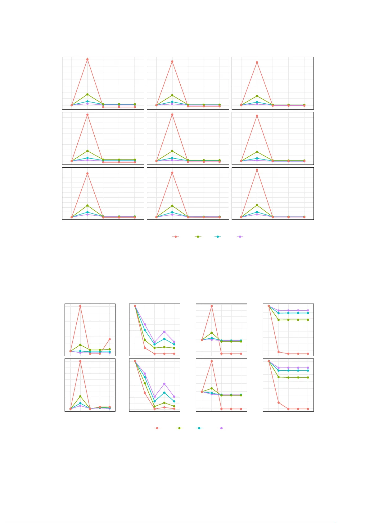
Multiv ariate GAR CH and p ortfolio v ariance prediction: a forecast reconciliation p ersp ectiv e Massimiliano Cap orin ∗ Departmen t of Statistical Sciences Univ ersity of P ado v a, Italy massimiliano.cap orin@unipd.it and Daniele Girolimetto Departmen t of Statistical Sciences Univ ersity of P ado v a, Italy daniele.girolimetto@unip d.it and Eman uele Lop etuso Departmen t of Statistical Sciences Univ ersity of P ado v a, Italy eman uele.lop etuso@unip d.it Marc h 19, 2026 Abstract W e assess the adv an tage of com bining univ ariate and m ultiv ariate portfolio risk forecasts with the aid of forecast reconciliation tec hniques. In our analyzes, w e assume knowledge of p ortfolio weigh ts, a standard for p ortfolio risk management applications. With an extensive sim ulation exp erimen t, we show that, if the true co v ariance is known, forecast reconciliation impro ves o ver a standard m ultiv ariate approac h, in particular when the adopted m ultiv ariate mo del is missp eciﬁed. Ho wev er, if noisy pro xies are used, correctly sp eciﬁed mo dels and the missp eciﬁed ones (for instance, neglecting spillov ers) turn out to b e, in several cases, indis- tinguishable, with forecast reconciliation still providing improv emen ts, even though smaller. The noise in the cov ariance pro xy plays a crucial role both in driving the improv ement of forecast reconciliation and in the identiﬁcation of the optimal mo del. An empirical analy- sis shows how forecast reconciliation can b e adopted with real data to improv e traditional GAR CH-based p ortfolio v ariance forecasts. Keyw ords: Multiv ariate GARCH, F orecast reconciliation, Portfolio Risk JEL: C58. ∗ Corresp onding author: Department of Statistical Sciences, Universit y of Pado v a, Via C. Battisti 241, 35121 P adov a, Italy - email: massimiliano.cap orin@unip d.it - phone: +39-049-827-4199. W e thank Eduardo Rossi, Juan-Angel Jimenez-Martin, Alfonso Nov ales, Esther Ruiz, Helena V eiga, Paolo San- tucci de Magistris, and the participants to the Italian Conference of Economic Statistics (SMEA) 2025, the Computational and Financial Econometrics conference 2025, and the seminars at Univrsidad Carlos I I I Madrid and Univ ersidad Complutense de Madrid for the suggestions, commen ts and stim ulating discussions. The authors ac knowledge ﬁnancial supp ort from pro ject PRIN2022 PRICE: A New Paradigm for High-F requency Finance, 2022C799SX. This study w as funded by the Europ ean Union-NextGeneration EU, Mission 4, Comp onent 2, in the framew ork of the GRINS-Growing Resilient, INclusive and Sustainable pro ject [grant num b ers GRINS PE00000018-CUP C93C22005270001]. 1 1 In tro duction Multiv ariate conditional heterosk edastic mo dels b elonging to the Generalized Auto Regressiv e Conditional Heterosk edasticity (MGAR CH) class are standard to ols in ﬁnancial econometrics. They represen t classic instrumen ts for a range of applications, from risk managemen t to hedging and asset allo cation; see surv eys b y Bau wens et al. (2005), Silv ennoinen and T erasvirta (2009), and F rancq and Zakoian (2019). Among the several sp eciﬁcations prop osed b y the literature (see the surveys previously cited for details), only a few are frequen tly adopted, and these include the Dynamic Conditional Correlation (DCC) mo del of Engle (2002), the Orthogonal GARCH (OGAR CH) mo del of Alexander (2002), and the Scalar BEKK of Ding and Engle (2001), which are feasible even in large dimensional cases. A relev ant c hallenge for MGARCH mo dels is, in fact, related to the so-called curse of dimensionality , that is, the large num b er of parameters of the most ﬂexible mo dels, whic h is sensibly limiting their use. F or instance, the BEKK mo del of Engle and Kroner (1995) is commonly considered only under strong parametric restrictions, suc h as in the just mentioned Scalar-BEKK case, while the VECH sp eciﬁcation (see again Engle and Kroner (1995)) has receiv ed limited atten tion in empirical analyzes. How ev er, restrictions imply a reduction in mo del ﬂexibility , whic h generally corresp onds to a limit in the interdependence across assets sho c ks and/or co v ariances (or correlations). This is in contrast with the empirical evidence suggesting that interdependence is presen t and relev an t, as demonstrated by the v arious w orks re-introducing limited ﬂexibilit y in MGARCH sp eciﬁcations; see, among many others, Cap orin and P aruolo (2015) and Billio et al. (2023). F rom a diﬀerent p erspective, the existence of interdependence is also at the base of the growing literature on systemic risk and ﬁnancial connectedness, originating from the seminal con tribution of Dieb old and Yilmaz (2009); see also (Dieb old and Yilmaz, 2023) and references therein cited. An asp ect not yet fully explored by the literature is the p ossibilit y of indirectly taking in to account the in terdep endence in a MGARCH framew ork and of exploiting its p oten tial in forecasting, thus paving the w ay for p ossible applications either in risk managemen t and p ortfolio allocation. Our intuition tak es the p oin t of view of a risk manager that has to ev aluate the risk (i.e., to predict the v ariance) of an existing p ortfolio. By construction, the weigh ts of the assets are kno wn, and if suﬃcien t historical data are av ailable for the returns or all the assets included in the p ortfolio, backw ard simulated, synthetic, p ortfolio returns can b e derived. The p ortfolio returns are then accoun ting for the interdependence across the assets risk (either in 2 terms of sho c ks or v ariance spillov ers), and this will be captured implicitly b y any univ ariate GAR CH-type mo del we might ﬁt on the p ortfolio returns. Of course, a univ ariate mo del might represen t a to o restrictive sp eciﬁcation, not taking prop erly into accoun t the heterogeneity in the dynamic of assets v ariances, cov ariances and/or correlations, something that could b e provided only by a MGAR CH mo del. F ortunately , the forecasting literature includes to ols for combining a ﬁt of a univ ariate mo del in a synthetic p ortfolio returns series, with a MGARCH mo del adapted to the collection of p ortfolio assets returns; w e refer to forecast reconciliation approaches (Hyndman et al., 2011; Wickramasuriy a et al., 2019; P anagiotelis et al., 2021; Di F onzo and Girolimetto, 2024; Girolimetto and Di F onzo, 2024; Girolimetto et al., 2023; A thanasop oulos et al., 2024). In this work, w e sho w that the prediction of the v ariance of a univ ariate GARCH mo del on p ortfolio returns can b e eﬃciently combined with the prediction of the cov ariance of an MGAR CH sp eciﬁcation to impro ve the prediction of a giv en p ortfolio risk. W e thus contribute b oth to the literature on forecast reconciliation, extending the application of its to ols in ﬁnance (see Cap orin et al., 2024 and Mattera et al. (2025)), and to the MGARCH literature, showing ho w assets interdependence can be accoun ted for. F or what concerns the forecast reconcilia- tion con tribution, we design a reconciliation approach tailored to the p ortfolio-v ariance setting, adapting shrink age-based metho ds to the aggregation constraints implied b y p ortfolio weigh ts. Our pro cedure ensures coherence and preserves the structure of the cov ariance matrix, making the reconciled forecasts more accurate and economically interpretable. Using simulations, we sho w ho w the com bination of univ ariate and multiv ariate forecasts improv es prediction accu- racy , in line with the ﬁndings of Wickramasuriy a et al. (2019) and P anagiotelis et al. (2021). Sp eciﬁcally , when fo cusing on the ﬁnancial econometrics side, in addition to the in tro duction of in terdep endence by means of a univ ariate ﬁt, we provide further contributions. First, w e sho w ho w the predictive p erformance of MGARCH mo dels might deteriorate under missp eciﬁcation. Second, and more relev ant, w e demonstrate that the use of noisy proxies masks the possible presence of interdependence, making MGARCH mo dels neglecting interdependence equiv alen t to the correctly sp eciﬁed ones. The pap er pro ceeds as follows. Section 2 is dev oted to the metho ds that sho w ho w forecast reconciliation can be used for portfolio v ariances, describing both the MGAR CH models and the forecast comparison to ols that we will consider. Section 3 rep orts the simulation design and the results, while Section 4 includes an empirical example with real data. Section 5 concludes 3 the pap er. An extensive Online App endix includes detailed results for the simulations and the empirical study . 2 Metho ds 2.1 F orecast reconciliation for portf olio v ariance As we noted in the in tro duction, the p ortfolio v ariance can be forecast either through a uni- v ariate approach applied directly to portfolio returns or via a b ottom-up strategy leveraging a m ultiv ariate mo del of asset returns. This dual structure provides an ideal setting for the application of forecast reconciliation techniques. W e ﬁrst deﬁne the framework we refer to. Assume that the interest is in the prediction of the p ortfolio v ariance for the next p erio d, a common need in ﬁnancial risk management. If this is the case, the p ortfolio comp osition is assumed to b e known. Therefore, in a setting where N assets are av ailable, w e denote by ω the (known) N − dimensional vector of p ortfolio weigh ts. W e also assume that the returns 1 of the N assets are av ailable ov er a common sample, that is, the N -dimensional vectors r t ∈ R N are observ ed for t = 1 , 2 , . . . , T . The goal is to pro duce a forecast of the p ortfolio v ariance for T + 1. Two approaches are commonly pursued. In the ﬁrst, one computes the p ortfolio returns r p,t = ω ′ r t and ﬁts a univ ariate GAR CH-type mo del to obtain the one-step-ahead forecast σ 2 p,T +1 of the p ortfolio v ariance. 2 In the second approach, a m ultiv ariate GARCH (MGARCH) mo del is ﬁtted to the asset return v ector r t , pro viding a forecast Σ T +1 of the conditional cov ariance matrix. Then, w e recov er the predicted p ortfolio v ariance by aggregating as γ 2 p,T +1 = ω ′ Σ T +1 ω . The presence of a reference forecast recov ered from a univ ariate approac h and of a second forecast obtained b y aggregation of a collection of elements (the predictions of asset v ariances and co v ariances) represen ts a standard situation in forecast reconciliation. Similar settings app ear in non-ﬁnancial applications such as hierarc hical forecasting in demography (Shang and Hyndman, 2017; Li et al., 2019), macro economic (P etrop oulos et al., 2014; Mircetic et al., 2022) energy (Silv a et al., 2018; W ang et al., 2021; Ab olghasemi et al., 2025). In the ﬁnancial literature, notable examples are Cap orin et al. (2024) and Mattera et al. (2025). T o simplify notation, all forecast quan tities are implicitly assumed to refer to the next p eriod, and the 1 F or simplicity , we assume that the returns are de-meaned. 2 F or simplicit y , we do not denote predicted quan tities with hats or conditioning on the av ailable information set, unless it is needed for clarity of the discussion. 4 time subscript T + 1 is omitted throughout the discussion of this subsection: σ 2 p,T +1 ≡ σ 2 p , γ 2 p,T +1 ≡ γ 2 p , Σ T +1 ≡ Σ and σ T +1 ≡ σ . Mo ving back to our setting, the prediction of p ortfolio v ariance using a univ ariate approach, namely σ 2 p , represents the so-called b ase forecast. The construction of the portfolio v ariance prediction by aggregation giv es the b ottom-up alternative γ 2 p , exploiting the informativ e conten t of the risk predictions coming from the single comp onen ts of the p ortfolio and accoun ting for their interdependence (measured by b oth the correlations and the links b et w een v ariances and co v ariances). In general, the base forecast and the b ottom-up forecast do not coincide, that is, σ 2 p  = γ 2 p . T o connect our framew ork with the results of the forecast reconciliation literature, w e express the b ottom-up forecast as a linear combination of the univ ariate underlying elements (v ariances and co v ariances) of Σ : γ 2 p = ω ′ Σ ω =  ω ′ ⊗ ω ′  D N ve ch ( Σ ) = Aσ , (1) where ve ch ( · ) denotes the half-v ectorization op erator, D N is the duplication matrix, 3 and σ is the vector of dimension m = N ( N +1) 2 collecting the diﬀerent elements of Σ . The matrix A = ( ω ′ ⊗ ω ′ ) D N (with size (1 × m )) is also called the aggr e gation (or linear com bination, Girolimetto and Di F onzo, 2024) matrix in the reconciliation literature (Hyndman et al., 2011). Then, the p ortfolio v ariance forecasts obtained from the univ ariate GARCH-t yp e approac h and from the MGARCH mo del can b e reconciled by solving the following generalized least squares problem: argmin e y ( y − e y ) ′ Ω ( y − e y ) sub ject to C e y = 0 , (2) with the solution given by (Stone et al., 1942; Byron, 1978, 1979): e y =  I m +1 − Ω C ′ ( C Ω C ′ ) − 1 C  y , where e y =  e γ 2 p e σ ′  ′ , y =  σ 2 p σ ′  ′ , C = [1 − A ] is the (1 × m + 1) constrain ts matrix, and Ω is a ( m + 1) × ( m + 1) p ositiv e deﬁnite matrix represen ting the co v ariance matrix of the (time series of ) forecast errors of b oth the b ottom-lev el comp onen ts (i.e., the elements of v ector σ t ) and the p ortfolio series (i.e., σ 2 p,t ). Sev eral approac hes ha v e b een prop osed in the literature to estimate Ω , see Athanasopoulos et al. (2024). How ev er, in this work, we consider 3 The duplication matrix satisﬁes ve c ( Σ T +1 ) = D N ve ch ( Σ T +1 ) with vec being the matrix vectorization op erator and has size  N 2 × N ( N +1) 2  . 5 the state-of-the-art shrink age estimators prop osed by Wic kramasuriya et al. (2019), based on the in-sample residuals of the individual forecasting mo dels (see, e.g., Hyndman et al., 2016; P anagiotelis et al., 2021; Cap orin et al., 2024). After reconciliation, the t wo p ortfolio v ariance forecasts coincide b y construction: e γ 2 p = e σ 2 p . 2.1.1 Reconciliation pro cedures and correlation matrix coherence After reconstructing the reconciled co v ariance matrix as e Σ = ve ch − 1 ( e σ ), the corresp onding correlation matrix e R may not satisfy the required prop erties of a prop er correlation matrix. In particular, it may contain oﬀ-diagonal elements with absolute v alues that exceed one, that is, | e ρ i,j | > 1, th us violating the mathematical deﬁnition of a correlation co eﬃcien t. Therefore, we prop ose tw o no vel reconciliation strategies designed to sp eciﬁcally address this issue: (A) Non-linear constrained optimization. Non-linear inequalit y constraints are introduced in the optimization problem 2 such that argmin e y ( y − e y ) Ω ( y − e y ) ′ s . t . C e y = 0 and    g ( y ) i  = j ≤ 1 g ( y ) i = i = 1 , with i, j = 1 , ..., N (3) where g ( e y ) is a function that extracts the correlation matrix from the reconciled co v ariance matrix e Σ and returns the absolute v alues of its elements in vectorized form: g ( e y ) =    ve ch  cor  e Σ     . This non-linear problem might b e solv ed, for instance, using the R pack age Rsolnp (Gha- lanos and Theussl, 2015). (B) Reconciliation via correlation decomp osition. Starting from equation (1), we decomp ose the b ottom-up p ortfolio v ariance a decomp osi- tion of the cov ariance γ 2 p = ω ′ Σ ω = ω ′ S RS ω =  ω ′ ⊗ ω ′  ( S ⊗ S ) D N ve ch ( R ) = A σ ρ , (4) where Σ = S RS is the conditional cov ariance matrix, where S = diag ( σ 1 , σ 2 , . . . , σ N ) is the diagonal matrix of conditional standard deviations of the N assets, 4 , and ρ = ve ch ( R ) 4 M = diag( m ) is the algebraic op erator creating a diagonal matrix M with the vector m b eing the set of diagonal elements. 6 is the v ector of correlations. It follows that the aggregation matrix A σ = ( ω ′ ⊗ ω ′ ) ( S ⊗ S ) D N dep ends on the con- ditional v ariances through S . Th us, once the reconciled vector e σ are obtained from equa- tion (1), we can reconstruct the reconciled cov ariance matrix e Σ = ve ch − 1 ( e σ T +1 ) and compute: e S = I N ⊙ diag( e Σ ) , e A σ =  ω ′ ⊗ ω ′   e S ⊗ e S  D N , e C σ =  1 − e A σ  . Reconciliation is then p erformed directly on correlations: argmin e x ( x − e x ) W ( x − e x ) ′ s . t . e C σ e x = 0 and    − 1 ≤ e ρ i  = j ≤ 1 e ρ i = j = 1 with i, j = 1 , ..., N (5) where e x = h e γ 2 p,T +1 e ρ T +1 i ′ denotes the reconciled forecast v ector, x = h σ 2 p,T +1 ρ T +1 i ′ collects the base forecast of the p ortfolio v ariance and the disaggregated correlation fore- casts, and W is a p ositiv e deﬁnite w eighting matrix represen ting the forecast error v ari- ance of the p ortfolio and the N assets. The quadratic programming problem with linear equalit y and inequality constraints (5) can b e solved using standard numerical optimiza- tion tec hniques, for instance those av ailable in the R pack age FoReco (Girolimetto and Di F onzo, 2025), whic h provides a ﬂexible implementation of reconciliation pro cedures within this framew ork. T aking into account the previous elements, we prop ose a method for reconciling p ortfolio v ariance forecasts to enhance the accuracy of risk estimation b y com bining univ ariate and m ultiv ariate approaches. The steps of this reconciliation pro cedure are describ ed in Algorithm 1. W e stress that the main ob jectiv e of our research is to determine if forecast reconciliation to ols lead to p otential improv emen ts in the prediction of p ortfolio v ariance. Moreo ver, we are also in terested in determining if, by exploiting the information contained in the direct p ortfolio v ariance prediction (based on univ ariate metho ds), we will improv e the prediction based on the commonly adopted MGARCH mo dels, whic h might be miss-sp eciﬁed due to the lac k of v ariance interdependence. In b oth cases, the ev aluation will compare the baseline p ortfolio 7 v ariance forecast with the b ottom-up one and forecast reconciliation, for a given pair of ﬁtted univ ariate GARCH and MGARCH sp eciﬁcations. Algorithm 1: F orecast reconciliation of p ortfolio v ariance Input: P ortfolio weigh ts ω ∈ R N , univ ariate (base) forecast for the p ortfolio v ariance σ 2 p , m ultiv ariate (base) forecast for the N assets cov ariance matrix Σ Output: Reconciled p ortfolio v ariance e γ 2 p , reconciled co v ariance matrix e Σ 1 Compute σ ← ve ch ( Σ ); 2 Compute aggregation matrix: A ← ( ω ′ ⊗ ω ′ ) D N ; 3 Deﬁne the base vector: y ←  σ 2 p σ  ; 4 Deﬁne constraint matrix: C ←  1 − A  ; 5 Solv e the generalized least squares problem (2): e y ←  e γ 2 p e σ  ; 6 Reconstruct reconciled cov ariance matrix: e Σ ← ve ch − 1 ( e σ ); 7 Compute correlation matrix: e R ← cor ( e Σ ); 8 if any oﬀ-diagonal element of e R violates | ρ i,j | > 1 then /* Option A: Non-linear constrained optimization */ 9 Solv e the non-linear constrained optimization problem (3): : e y ←  e γ 2 p e σ  ; 10 Reconstruct reconciled co v ariance matrix: e Σ ← ve ch − 1 ( e σ ); /* (B) Reconciliation via correlation decomposition */ 11 Compute ρ ← ve ch ( R ) with R ← cor ( Σ ); 12 Compute e S = I N ⊙ diag( e Σ ) 1 / 2 ; 13 Compute mo diﬁed aggregation matrix: e A σ ← ( ω ′ ⊗ ω ′ )( e S ⊗ e S ) D N ; 14 Deﬁne the base vector using correlation forecasts: x ←  σ 2 p ρ  ; 15 Deﬁne constrain t: e C σ ← h 1 − e A σ i ; 16 Solv e the linear constrained optimization problem (5): e x =  e γ 2 p e ρ  ; 17 Reconstruct reconciled correlation and cov ariance matrix: e R ← ve ch − 1 ( e ρ ) and e Σ ← e S e R e S 18 end 19 return e γ 2 p and e Σ ; 2.2 Univ ariate and Multiv ariate GAR CH mo dels As mentioned in the previous section, the construction of reconciled forecasts for the p ortfolio v ariance, starting from either portfolio or asset returns, requires the sp eciﬁcation of a univ ariate mo del for the former and of a m ultiv ariate mo del for the latter. F or simplicity , in the case of the p ortfolio returns, we sp ecify a simple GARCH(1,1) mo del: 8 σ 2 p,t = ω + αr 2 p,t − 1 + β σ 2 p,t − 1 . (6) W e are a ware that a more standard approac h is now given by a mo del with asymmetry in the v ariances, but we prefer to maintain no w the coherence in the features captured by the mo del providing the base forecast and the m ultiv ariate mo del b ehind the b ottom-up forecast. F urther generalizations are left for future work. Mo ving to the Multiv ariate GARCH mo dels used to pro duce forecasts, we restrict our at- ten tion to tw o sp eciﬁc cases: the BEKK mo del of Engle and Kroner (1995) and the Dynamic Conditional Correlation (DCC) mo del of Engle (2002). F or the BEKK mo del, we consider the simplest sp eciﬁcation: Σ t = C C ′ + A r t − 1 r ′ t − 1 A + B Σ t − 1 B ′ , (7) where C is low er triangular, while A and B should b e full matrices. How ever, in empirical studies, to deal with the so-called curse of dimensionality , b oth A and B are restricted to b e diagonal or even driv en b y a single parameter, see, among man y others, Engle and Kroner (1995); Ding and Engle (2001); Cap orin and McAleer (2008). The second mo del builds on the DCC dynamic for correlations, accompanied b y a p eculiar dynamic ov er marginals to allow, p oten tially , for v ariance in terdep endence. The mo del we con- sider might b e seen as a sp ecial case of the V ector ARMA-GARCH of Ling and McAleer (2003) with DCC dynamic, and has b een prop osed, in the case of constan t conditional correlation, b y He and T er¨ asvirta (2004), and b y Cap orale et al. (2014) for the DCC mo del. Our target is to maintain mo del feasibility (that is, allo wing for parameter estimation in a tw o-step pro ce- dure, ﬁrst univ ariate GAR CH on the marginals and then the correlation dynamic) and to allow for in terdep endence, limiting attention to p ositiv e spillov er eﬀects; the generalization allo wing for negative parameters as in Conrad and Karanasos (2010) is left to future research. In our sim ulations, the univ ariate mo dels for the single assets are thus sp eciﬁed as follo ws: σ 2 i,t = ω i + β i σ 2 p,t − 1 + n X j =1 α j r 2 j,t − 1 , i = 1 , 2 , . . . n. (8) W e deﬁne the standardized innov ations η i,t = σ − 1 i,t r i,t − 1 for i = 1 , 2 , . . . n and then sp ecify a 9 DCC mo del Q t = (1 − θ 1 − θ 2 ) Γ + θ 1 η t − 1 η ′ t − 1 + θ 2 Q t − 1 (9) Γ t =  ˜ Q t  − 1 Q t  ˜ Q t  − 1 ˜ Q t = diag ( σ 1 ,t , σ 2 ,t , . . . , σ n,t ) . In the follo wing, we refer to this mo del as Extended DCC (DCC with v ariance in teraction, EDCC). In the simulations, we will also consider the restricted sp eciﬁcations of b oth the BEKK and the DCC mo dels. In detail, we will consider the BEKK mo del with scalar parameters and the baseline DCC mo del without interactions (i.e., the marginals are simple GARCH(1,1)). F ollo wing the standard practice, the mo dels are estimated b y Quasi Maximum Lik eliho o d, and in the case of the DCC sp eciﬁcation using a m ulti-step pro cedure, starting from the marginals, then the Γ matrix (with a sample correlation estimator on η t ), and ﬁnally the parameters go verning the correlation dynamic. 2.3 F orecast comparison metho ds In this section, we describ e the metho dologies used to compare the forecast p erformance of diﬀeren t p ortfolio v ariance forecast approac hes. These metho ds include the accuracy of the p oin t forecast using b oth absolute and relative indicators, and emplo y hypothesis testing based on tw o diﬀeren t w ell-kno wn statistical pro cedures: the Diebold and Mariano (1995) test and the Mo del Conﬁdence Set (Hansen et al., 2011). Fiv e diﬀerent approac hes are compared based on their accuracy in forecasting the p ortfolio v ariance. These approac hes include b oth univ ariate and m ultiv ariate mo dels, as w ell as dif- feren t reconciliation tec hniques, aligning with the steps described in Algorithm 1 for forecast reconciliation. The approac hes considered are as follows: b ase The univ ariate model forecast for the p ortfolio v ariance, denoted as σ 2 p in Section 2.1. This approac h assumes that the v ariance of the p ortfolio can b e estimated from the historical data of p ortfolio returns. bu The b ottom-up approach using a m ultiv ariate mo del for the p ortfolio v ariance, expressed as γ 2 p = ω ′ Σ ω in Section 2.1. It ﬁrst forecasts the v ariances and cov ariances of the individual assets and then combines these to estimate the ov erall p ortfolio v ariance. 10 shr The optimal linear reconciliation (in a least squares sense), computed using the expression (2), denoted as e γ 2 p . This metho d inv olv es reconciling forecasts from the univ ariate p ortfolio v ariance forecasts and the v ariance and cov ariance matrix of the N assets. shr A This is an extension of the reconciliation approach shr , which addresses p otential issues arising when the correlation matrix e R contains oﬀ-diagonal elemen ts violating the con- dition | ρ i,j | > 1; see Section 2.2.1 and Option A in Algorithm 1. It applies a non-linear constrained optimization metho d to adjust the forecast correlation matrix, ensuring that all correlations remain within the feasible range of [ − 1 , 1]. shr B This is an extension of the reconciliation approach shr , where reconciliation is p erformed via a correlation decomp osition approach; see Section 2.2.2 and Option B in Algorithm 1. Here, we apply reconciliation using the correlation decomp osition (4) and solving the linear optimization problem (5). This metho d pro vides a more computational eﬃcient alternativ e to shr A . T o ev aluate the point forecast accuracy of the diﬀeren t mo dels, w e employ three widely used metrics:the Mean Squared Error (MSE, Davydenk o and Fildes, 2013), the Mean Absolute Error (MAE, Davydenk o and Fildes, 2013), and the Quasi-Lik eliho o d score (QLIKE, P atton, 2011; Cap orin et al., 2024). Eac h of these metrics provides a distinct p ersp ectiv e on the accuracy of the predicted v ariance. The expressions for these measures are giv en by the following: MSE j,q = 1 M M X i =1  σ 2 − γ 2 i,j,q  2 , (10) MAE j,q = 1 M M X i =1   σ 2 − γ 2 i,j,q   , (11) QLIKE j,q = 1 M M X i =1 " σ 2 γ 2 i,j,q − log σ 2 γ 2 i,j,q ! − 1 # , (12) where σ 2 denotes the true v alue, M denotes the size of the test set, 5 Q denotes the n umber of replications, 6 and γ 2 i,j,q refers to the p ortfolio v ariance forecast from approac h approach j (with j either base , bu , shr , shr A , or shr B ). W e note that while MSE and MAE are symmetric loss functions, QLIKE is asymmetric, with a larger loss asso ciated to under-prediction. T o obtain the o verall accuracy measures, we compute the a verage of each metric across all replications: IND = 1 Q Q X q =1 IND j,q , 5 This is set to 250 for sim ulations in Section 3, and 4037 for applications in Section 4. 6 W e use (500 for sim ulations in Section 3 and 1 for the application in Section 4. 11 and for relativ e accuracy (Davydenk o and Fildes, 2013), we calculate: AvgRelIND x =   Q Y q =1 IND j,q IND x,q   1 Q , where x ∈ { base, bu } and IND represents one of the ev aluation metrics (MSE, MAE, or QLIKE). Sp eciﬁcally , AvgRelIND bu and AvgRelIND base are t w o relativ e indicators that sho w an impro ve- men t in forecast compared to the bu and b ase models, resp ectiv ely . In addition to these ov erall and relativ e measures, w e conduct h yp othesis testing to compare forecast accuracy across diﬀeren t mo dels. W e emplo y the Dieb old and Mariano Diebold and Mariano (1995) (DM) test to ev aluate the null hypothesis of equal predictive accuracy (EP A) b et w een comp eting mo dels, with an ov erall signiﬁcance level set at α = 0 . 05. T o account for m ultiple pairwise comparisons, the DM test is implemen ted using the Bonferroni correction (Dunn, 1961). In addition, we apply the Mo del Conﬁdence Set (MCS) pro cedure prop osed by Hansen et al. (2011) to identify the subset of mo dels that cannot b e statistically distinguished in terms of forecast accuracy , rep orting results at conﬁdence lev els of 70%, 75%, 80%, 85%, 90% and 95%. These tests are crucial in determining whether the observed diﬀerences in forecast p erformance are statistically signiﬁcant or are merely due to randomness in the data. In the following sections, w e will consider the forecast comparison for b oth simulated and observ ed data. In the ﬁrst case, the true p ortfolio v ariance σ 2 is kno wn and will b e used to ev aluate the comp eting approaches. Ho wev er, with real data, the true v ariance is not observ ed and a pro xy m ust b e used. Two solutions are commonly considered, the ﬁrst b eing squared observ ed de-meaned returns. As sho wn by Patton and Sheppard (2009) for the univ ariate case and Laurent et al. (2013) for m ultiv ariate mo dels, this noisy pro xy might lead to non-robust mo del selection for some loss functions, in particular for the MAE (while MSE and QLIKE are loss functions robust the presence of noise in the proxy). An alternative proxy might b e reco vered using high frequency data, and the daily v ariance (cov ariance) is estimated using the Realized V ariance (Realized Cov ariance). Giv en the complexity of sim ulating high frequency data under a Multiv ariate GAR CH mo del, we c hose to ﬁrst consider the noisy proxy in the sim ulation experiments, and then to mimic the existence of a b etter proxy by con taminating with additive noise the true co v ariance. In contrast, realized meas ures will be used, together with the squared returns, as proxies for the unknown v ariance when considering real data. 12 3 Sim ulations 3.1 Sim ulation design W e consider sev eral scenarios with v arying sample sizes and n umber of v ariables. In particular, sim ulated return series are generated for portfolios comprising 9 and 24 assets using four distinct data generating processes: a fully parametrized BEKK, a scalar BEKK, the standard DCC- GAR CH, and the EDCC-GAR CH (incorp orating in teractions). W e begin by illustrating the DGP used in the simulations for the case of 9 assets. The cov ariance matrix in the full BEKK sp eciﬁcation is generated according to equation (7) and setting r t = Σ 1 2 t z t with z t sampled from a Multiv ariate Normal density with zero mean and co v ariance equal to the identit y matrix. In terms of parameters, this formulation represents the most general approach, capturing a broad range of interdependencies. In contrast, the scalar BEKK restricts the dynamics by imp osing that the matrices A and B assume the forms √ αI and √ β I , resp ectiv ely , where α and β are scalars and I denotes identit y . In the scalar BEKK mo del, co v ariance stationarity is guaranteed when α + β < 1. Accord- ingly , in each simulation w e draw α ∼ U (0 . 05 , 0 . 20) and β ∼ U (0 . 70 , 0 . 95). W e then verify the stationarit y condition and, if α + β ≥ 1, we redraw the parameters until α + β < 1 holds. In the full BEKK, the cov ariance stationarity condition dep ends on the eigenv alues: P k ( A ⊗ A ) D k + P k ( B ⊗ B ) D k whic h are required to b e strictly b elo w unit y in modulus; in the previous equation D k represen ts the duplication matrix of size k and P k its generalized in verse. 7 W e considered sp eciﬁc designs for the B matrix. In particular, w e partition B into 3 × 3 blo c ks and, for eac h diagonal blo ck, w e set the entries as follows: the main-diagonal elements are drawn from a uniform distribution on [0 . 70 , 0 . 95], whereas the oﬀ-diagonal elements are dra wn from a uniform distribution on [0 , 0 . 10]. In contrast, A is generated without imp osing an y blo c k structure, and all of its en tries are drawn from a uniform distribution on [0 , 0 . 10]. After generating A and B , w e c hec k the stationarity conditions; if they are not satisﬁed, the parameter dra w is discarded and the matrices are resampled un til the conditions hold. This pro cedure is rep eated indep enden tly for each simulation. F or b oth scalar and full BEKK mo dels, the matrix C is generated as a lo wer triangular 7 The duplication matrix D k satisﬁes ve c ( M ) = D k ve ch ( M ) for a k − dimensional square symmetric matrix M . 13 matrix with random entries, constructed to ensure that the pro duct C C ′ main tains full rank and has a p ositiv e diagonal. The remaining generators are based on the DCC-GARCH framework, as given in (8) and (9). Similarly to the BEKK case, we randomly draw parameters. In each simulation, the parameters gov erning the correlation dynamics are dra wn from uniform distributions, with θ 1 ∼ U (0 . 05 , 0 . 30) and θ 2 ∼ U (0 . 70 , 0 . 85). T o enforce stationarity , we discard the draw if the condition θ 1 + θ 2 < 1 is not satisﬁed and resample the parameters un til it holds. Moreo ver, the elemen ts of Γ are generated as follo ws: ﬁrst, w e sample a matrix A of random Normal num b ers with mean − 0 . 15 and standard deviation 0 . 6; then we compute Q = A ′ A , and normalize it so that it has unit elemen ts on the main diagonal; ﬁnally , we set Γ = 0 . 5 ( Q + Q ′ ) and retain the sim ulated matrix only if the smallest eigenv alue is larger than 1 e − 10. The initial generation of random n umbers ensures that the a verage correlation level is slightly higher than 0 . 4. The diﬀerence b et ween the standard DCC-GARCH and the v arian t with interactions lies in the sp eciﬁcation of individual dynamics. In the simpler DCC mo del, the evolution of v ari- ances follo ws (8), with the DCC-GAR CH co eﬃcien ts α i and β i sampled from the distributions α i ∼ U (0 . 05 , 0 . 15) and β i ∼ U (0 . 7 , 0 . 85), with β j = 0 for j  = i . In the mo del incorp orating in teractions, we represent the collection of v ariances in a matrix form as σ 2 t = ω + A r 2 t − 1 + B σ t , where σ 2 t is the vector of v ariances, B is diagonal and A is unrestricted, p ermitting nonzero oﬀ-diagonal elements. The diagonal entries for A and B are selected from uniform distributions in [0 , 0 . 2] and [0 . 7 , 0 . 85], resp ectiv ely , while the oﬀ-diagonal elemen ts of A are dra wn from U (0 , 0 . 02). The co eﬃcien ts are generated repeatedly un til the eigen v alues of A + B are all within the unit circle, th us guaran teeing cov ariance stationarit y as discussed in Ling and McAleer (2003). F or the simulations with 24 assets, we adopt ﬁxed coeﬃcient designs. F or models suc h as the full BEKK, drawing fully random parameter matrices that (i) satisfy co v ariance stationarity and (ii) yield reasonable parameter v alues (e.g., larger and p ositive diagonal en tries) w ould typically require rep eated draws for each simulation, substan tially increasing the computational burden. W e therefore ﬁx the parameters of the data-generating pro cesses. Sp eciﬁcally , in the scalar BEKK w e set α = 0 . 15 and β = 0 . 80. In the full B EKK, the 14 co eﬃcien t matrices A and B are set to B = I 8 ⊗       0 . 80 0 . 05 0 . 05 0 . 05 0 . 80 0 . 05 0 . 05 0 . 05 0 . 80       , A =        0 . 025 1 8 × 8 0 . 0125 1 8 × 8 0 · 1 8 × 8 0 . 0125 1 8 × 8 0 . 0187 1 8 × 8 0 . 025 1 8 × 8 0 . 0187 1 8 × 8 0 . 0125 1 8 × 8 0 . 0312 1 8 × 8        . F or the DCC–GAR CH mo del, w e set θ 1 = 0 . 15 and θ 2 = 0 . 80, and w e ﬁx the univ ariate GAR CH parameters to α i = 0 . 15 and β i = 0 . 80 for all i . In the model incorporating in teractions, w e c ho ose θ 1 and θ 2 analogously , and w e set B accordingly . Con versely , the matrix A is speciﬁed with 0 . 08 on the main diagonal and 0 . 05 elsewhere. Giv en the parameters, we simulate returns sequences from the v arious data generating pro- cesses, also storing the true conditional co v ariance and correlation matrices. Subsequen tly , on the returns sim ulated from each DGP , w e estimate three m ultiv ariate mo dels, the Scalar BEKK, a standard DCC-GAR CH, and the extended DCC (EDCC); the last mo del is not estimated in all cases. In addition, w e aggregate the multiv ariate returns into a p ortfolio, either using equal w eights, 1 /n , where n denotes the total num b er of assets (8 or 24), or with randomly generated w eights (ensuring that their sum equals 1). On the p ortfolio returns, we estimate a univ ariate GAR CH mo del. F or each scenario, 100 + T + 250 observ ations are sim ulated, the ﬁrst 100 are then discarded to av oid dep endence on starting v alues, T are employ ed for mo del estimation and the ﬁnal 250 reserv ed for out-of-sample ev aluation. All forecasts are one-step ahead, meaning that Σ t +1 is estimated using the observed return r t . F or the p ortfolios with 24 assets we set T = 1000, while for the 9-asset scenario we also consider the alternative sample sizes of T = 500 and T = 2000. F or all sim ulation designs, we p erformed 500 exp erimen ts. 3.2 Results In this subsection, we analyze the simulation results. W e ﬁrst fo cus on univ ariate v ersus mul- tiv ariate mo dels, then highligh t the b eneﬁts of forecast reconciliation, and later discuss the impact of a noisy pro xy . W e stress that we are not contrasting ﬁtted DCC to ﬁtted BEKK or EDCC but rather con trasting the p ortfolio v ariance forecast from a univ ariate GAR CH to those of a MGAR CH mo del and the forecast reconciliation based on the giv en MGARCH. 15 3.2.1 Base vs. b ottom-up: DGPs without in terdep endence W e start by con trasting the p ortfolio v ariance forecasts made following a b ottom-up approac h ( bu ), that is, estimating a MGAR CH mo del, with those obtained b y directly w orking on the p ortfolio returns, that is, with a univ ariate GAR CH mo del ( b ase ). A t ﬁrst we consider a cor- rectly sp eciﬁed MGAR CH model and lo ok at the relativ e accuracy indexes setting the univ ariate mo del as the reference (with a relative index thus equal to 1): see T able 1, columns lab eled b ase and bu ; full results including the v alue of the accuracy indexes are rep orted in the Online App endix. Notably , if we estimate a correctly speciﬁed MGAR CH model, the prediction of p ortfolio risk is closer to the true v alue than the one obtained from a univ ariate GAR CH mo del (miss- sp eciﬁed) ﬁt on p ortfolio returns, that is, w e observe a v alue low er than 1 for the bu case. Note that, as rep orted in the App endix, the accuracy measures decrease with the sample size in all cases, as exp ected. The pattern observed on relativ e accuracy , lo w er bu v alues, do es not depend on the p ortfolio w eigh ts (equal or randomly generated), on the sample size, and on the accuracy measure. W e observe that, for the Scalar-BEKK DGP , the preference for the b ottom-up approac h is attenuated as the sample size increases (the bu v alues increase) and is, o verall, less pronounced than in the DCC-GAR CH case. W e interpret this as a consequence of aggregating returns generated under a Scalar-BEKK mo del with Gaussian inno v ations. In fact, if returns follow r t |I t − 1 ∼ N ( 0 , Σ t ), with I t − 1 b eing the time t − 1 information set, and we set the p ortfolio weigh ts to b e time-inv ariant, ω (and summing up to one), we ha ve ω ′ Σ t ω = σ 2 p,t = ω ′ C C ′ ω + α ω ′ r t − 1 r ′ t − 1 ω + β ω ′ Σ t − 1 ω = ˜ c + α r 2 t − 1 + β σ 2 p,t − 1 with r t − 1 b eing the returns of the portfolio (a w eighted a verage). The preference of the MGAR CH sp eciﬁcation for shorter samples migh t b e linked to the larger amoun t of infor- mation used for parameters estimation ( N series against 1) an eﬀect that tends to disapp ear asymptotically , as suggested b y the closer p erformances for T = 2000 with random weigh ts. A similar aggregation result do es not hold for the DCC-GAR CH mo del due to the heterogeneity in the volatilit y dynamic and the standardization required to obtain the dynamic correlations. In line with this pattern, for increasing sample size, the p erformance of the correctly sp eci- ﬁed MGARCH improv es, with bu v alues decreasing with T . Ov erall, these ﬁrst outcomes are 16 T = 500 T = 1000 T = 2000 Index b ase bu shr shr A shr B b ase bu shr shr A shr B b ase bu shr shr A shr B DGP and Fitted mo del: Scalar BEKK - P ortfolio weigh ts 1 / N MSE 1.000 0.408 0.156 0.156 0.158 1.000 0.427 0.207 0.207 0.212 1.000 0.504 0.276 0.276 0.280 MAE 1.000 0.665 0.385 0.385 0.385 1.000 0.686 0.458 0.458 0.459 1.000 0.739 0.541 0.541 0.542 QLIKE 1.000 0.418 0.158 0.158 0.161 1.000 0.433 0.210 0.210 0.213 1.000 0.504 0.278 0.278 0.281 DGP and Fitted mo del: Scalar BEKK - P ortfolio weigh ts: random MSE 1.000 0.397 0.153 0.153 0.155 1.000 0.411 0.189 0.189 0.190 1.000 0.495 0.276 0.276 0.280 MAE 1.000 0.658 0.382 0.382 0.383 1.000 0.667 0.434 0.434 0.434 1.000 0.734 0.543 0.543 0.544 QLIKE 1.000 0.409 0.157 0.157 0.159 1.000 0.416 0.192 0.192 0.192 1.000 0.496 0.279 0.279 0.282 DGP and Fitted mo del: DCC-GAR CH - Portfolio w eights: 1 / N MSE 1.000 0.285 0.233 0.233 0.234 1.000 0.200 0.173 0.173 0.173 1.000 0.126 0.111 0.111 0.111 MAE 1.000 0.534 0.495 0.494 0.495 1.000 0.459 0.432 0.432 0.433 1.000 0.371 0.352 0.352 0.352 QLIKE 1.000 0.278 0.251 0.251 0.251 1.000 0.209 0.193 0.193 0.193 1.000 0.142 0.132 0.132 0.133 DGP and Fitted mo del: DCC-GAR CH - Portfolio w eights: random MSE 1.000 0.291 0.238 0.238 0.238 1.000 0.212 0.180 0.180 0.180 1.000 0.142 0.119 0.119 0.119 MAE 1.000 0.543 0.503 0.503 0.503 1.000 0.469 0.439 0.439 0.439 1.000 0.391 0.365 0.365 0.365 QLIKE 1.000 0.292 0.265 0.265 0.265 1.000 0.216 0.198 0.198 0.198 1.000 0.154 0.140 0.140 0.140 T able 1: Average relativ e accuracy indexes where the reference forecast is the univ ariate GARCH ﬁtted on simulated p ortfolio returns, and the DGP is either the Scalar BEKK (ﬁrst and second panels) or the DCC-GARCH (third and fourth panels). The top rows rep ort the sample size ( T ) and the v ariance forecast approach, including the univ ariate GARCH on p ortfolio returns, b ase , the b ottom-up approac h using MGARCH mo dels, bu , and the three forecast reconciliation cases discussed in the previous section. The ﬁrst and third panels consider equally weigh ted p ortfolios (the 1 / N case), while the second and fourth consider random p ortfolio weigh ts. All v alues are av erages across 500 replications. In each row, the b est and second b est forecast approaches are in b old and italic, resp ectively . 17 somewhat exp ected. Results start to b e more in teresting if w e consider a misspeciﬁed model, still focusing only on DGPs without an y form of interdependence; see T able 2, again columns lab eled b ase and bu . In terms of levels of accuracy indexes, they decrease with increasing sample size (as exp ected); see the App endix. Mo ving to relative indicators, if we estimate a Scalar BEKK on series generated from a DCC-GAR CH, and fo cus on small sample sizes, the wrongly sp eciﬁed model is providing sup erior forecasts compared to a univ ariate GARCH ﬁtted on portfolio returns. How ev er, as the sample size increases, the b ase and bu approaches tend to con verge, and then bu starts deteriorating with resp ect to b ase . This b eha viour do es not dep end on p ortfolio weigh ts. The outcome is diﬀerent if the DGP is a Scalar BEKK and the ﬁtted mo del is a DCC-GARCH: the univ ariate mo del on portfolio returns is inferior to the misspeciﬁed MGAR CH irrespective of the sample size (and again this do es not dep end on the p ortfolio weigh ts). W e link such evidence, again, to the aggregation of Scalar BEKK into a univ ariate GARCH on p ortfolio returns. In this case, the DCC-GAR CH is clearly miss-sp eciﬁed but its heterogeneit y helps in capturing the diﬀerences in unconditional v ariances (as driven by the diﬀerences across elements in the in tercept). Extending the cross-sectional dimension from N = 9 to N = 24 produces some notable shifts in the simulations. Under correctly sp eciﬁed estimation, when the DGP is DCC-GARCH, the univ ariate baseline no w outp erforms the correctly sp eciﬁed m ultiv ariate mo del—rev ersing the N = 9 ranking. By con trast, when the DGP is Scalar BEKK, the correctly sp eciﬁed m ultiv ariate mo del contin ues to dominate the univ ariate b enchmark, in line with the N = 9 evidence. Under missp eciﬁcation, dimensionality also resh uﬄes the cross-cases. If the DGP is Scalar BEKK but the estimation is p erformed with DCC-GAR CH, the m ultiv ariate sp eciﬁcation p er- forms b etter at N = 24 as in the N = 9 case. Conv ersely , if the DGP is DCC-GARCH and the multiv ariate estimator is a Scalar BEKK, the univ ariate baseline is now preferred. Overall, mo ving from nine to tw en ty-four assets strengthens the bias–v ariance trade-oﬀ and aggregation eﬀects, ero ding the adv an tage of correctly speciﬁed high-dimensional DCC in one case while preserving the edge of Scalar BEKK in the other. Results referring to the N = 24 case are a v ailable in the Online App endix. 18 T = 500 T = 1000 T = 2000 Index b ase bu shr shr A shr B b ase bu shr shr A shr B b ase bu shr shr A shr B DGP: DCC-GAR CH - Fitted mo del: Scalar BEKK - Portfolio weigh ts 1 / N MSE 1.000 0.686 0.595 0.595 0.594 1.000 0.861 0.760 0.760 0.760 1.000 1.002 0.851 0.852 0.852 MAE 1.000 0.848 0.788 0.788 0.788 1.000 0.954 0.888 0.888 0.888 1.000 1.024 0.935 0.935 0.936 QLIKE 1.000 0.763 0.681 0.681 0.681 1.000 0.953 0.846 0.846 0.846 1.000 1.074 0.927 0.927 0.928 DGP: DCC-GAR CH - Fitted mo del: Scalar BEKK - Portfolio weigh ts: random MSE 1.000 0.676 0.559 0.558 0.558 1.000 0.885 0.738 0.738 0.738 1.000 1.104 0.857 0.857 0.857 MAE 1.000 0.843 0.766 0.766 0.766 1.000 0.963 0.875 0.875 0.875 1.000 1.065 0.941 0.941 0.941 QLIKE 1.000 0.756 0.645 0.645 0.645 1.000 0.961 0.819 0.819 0.820 1.000 1.153 0.939 0.939 0.940 DGP: Scalar BEKK - Fitted mo del: DCC-GAR CH - Portfolio weigh ts: 1 / N MSE 1.000 0.773 0.428 0.428 0.444 1.000 0.784 0.477 0.477 0.492 1.000 0.780 0.489 0.489 0.495 MAE 1.000 0.878 0.646 0.646 0.649 1.000 0.899 0.696 0.696 0.699 1.000 0.893 0.716 0.716 0.717 QLIKE 1.000 0.786 0.435 0.435 0.452 1.000 0.799 0.487 0.487 0.496 1.000 0.786 0.494 0.494 0.498 DGP: Scalar BEKK - Fitted mo del: DCC-GAR CH - Portfolio weigh ts: random MSE 1.000 0.839 0.455 0.455 0.459 1.000 0.788 0.485 0.485 0.492 1.000 0.815 0.526 0.526 0.527 MAE 1.000 0.915 0.666 0.666 0.667 1.000 0.895 0.702 0.702 0.703 1.000 0.917 0.742 0.742 0.742 QLIKE 1.000 0.857 0.468 0.468 0.473 1.000 0.800 0.495 0.495 0.503 1.000 0.824 0.533 0.533 0.534 T able 2: Average relativ e accuracy indexes where the reference forecast is the univ ariate GARCH ﬁtted on sim ulated portfolio returns, and the DGP is either the DCC-GARCH (ﬁrst and second panels) or the Scalar BEKK (third and fourth panels). The ﬁtted MGARCH mo dels are missp eciﬁed (and still without interdependence): w e estimate the Scalar BEKK under the DCC-GAR CH DGP , and the DCC-GARCH with data generated from a Scalar BEKK. the The top rows rep ort the sample size ( T ) and the v ariance forecast approach, including the univ ariate GARCH on p ortfolio returns, b ase , the b ottom-up approach using MGAR CH mo dels, bu , and the three forecast reconciliation cases discussed in the previous section. The ﬁrst and third panels consider equally w eighted p ortfolios (the 1 / N case), while the second and fourth consider random p ortfolio weigh ts. All v alues are av erages across 500 replications. In each row, the b est and second b est forecast approac hes are in b old and italic, resp ectiv ely . 19 3.2.2 Base vs. b ottom-up: DGPs with in terdep endence Consider no w the tw o DGPs that include interdependence, namely , the EDCC-GARCH and the BEKK mo dels. Ev en in this case, w e estimate the t wo sp eciﬁcations without in terdep en- dence, the DCC-GAR CH and the Scalar BEKK, and we con trast the p ortfolio v ariance forecast obtained from a univ ariate GAR CH with that of the misspeciﬁed MGAR CH mo dels; see T a- bles 3 and 4, still fo cusing only on columns b ase and bu . F or completeness, w e also estimate the correctly sp eciﬁed mo del under the EDCC-GAR CH DGP (the fully parameterized BEKK estimation remains computationally unfeasible). F or the BEKK DGP the univ ariate mo del is pro viding sup erior forecast abilities compared to either the Scalar BEKK and the DCC-GAR CH. Moreo ver, the p erformance of MGAR CH mo dels worsens, in relativ e terms, with increasing sam- ple size. This is v alid irresp ectiv e of the loss function considered. On the other hand, for the EDCC-GAR CH DGP , the use of a missp eciﬁed DCC-GAR CH provides b etter forecasts than a univ ariate mo del on p ortfolio returns. This is in striking contrast with the result of the ﬁtted Scalar BEKK (on the EDCC-GAR CH DGP) whose forecasts are clearly inferior to those of the univ ariate mo del for sample size abov e 1000. W e link such a ﬁnding to the relatively limited size of the co eﬃcien ts of other asset sho cks in the EDCC-GARCH DGP . The correctly sp eciﬁed mo del clearly fa vors the b ottom-up approac h compared to the univ ariate baseline. All results are equiv alent for equally w eigh ted portfolios and randomly generated p ortfolios. See the Online App endix for detailed results for b oth the N = 9 and the N = 24 cases. Re-running the sim ulations with N = 24 assets yields patterns broadly consistent with the N = 9 case when the DGP is a BEKK: the baseline univ ariate forecast (base) remains preferable to the b ottom-up aggregation (bu), with the gap esp ecially pronounced when the estimated m ultiv ariate mo del is a Scalar BEKK. By con trast, under the EDCC–GAR CH DGP , mo ving to N = 24 makes the univ ariate estimate outp erform the b ottom-up approach b oth when the m ultiv ariate estimator is Scalar BEKK and when it is a standard DCC–GAR CH. Ov erall, higher dimensionalit y ampliﬁes estimation risk and missp eciﬁcation costs in parsimonious m ultiv ariate structures, k eeping the univ ariate baseline a particularly comp etitiv e b enc hmark at N = 24. 3.2.3 F orecast reconciliation T ables from 1 to 4 con tain the results of the three forecast reconciliation approaches that we consider. F rom the estimation of the correctly sp eciﬁed MGARCH mo del without interdepen- dence (T able 1), we ha v e a ﬁrst interesting result: in terms of relative forecast accuracy indexes, 20 T = 500 T = 1000 T = 2000 Index b ase bu shr shr A shr B b ase bu shr shr A shr B b ase bu shr shr A shr B DGP: F ull BEKK - Fitted mo del: Scalar BEKK - P ortfolio weigh ts 1 / N MSE 1.000 19.151 0.663 0.663 0.663 1.000 23.737 0.742 0.742 0.742 1.000 27.699 0.786 0.786 0.786 MAE 1.000 4.745 0.897 0.897 0.897 1.000 5.449 0.941 0.941 0.941 1.000 5.994 0.963 0.963 0.963 QLIKE 1.000 21.092 1.148 1.169 1.148 1.000 27.143 1.229 1.228 1.228 1.000 32.571 1.209 1.214 1.209 DGP: F ull BEKK - Fitted mo del: Scalar BEKK - P ortfolio weigh ts: random MSE 1.000 11.402 0.761 0.761 0.761 1.000 13.696 0.810 0.810 0.810 1.000 15.417 0.832 0.832 0.832 MAE 1.000 3.643 0.930 0.930 0.930 1.000 4.055 0.956 0.956 0.956 1.000 4.371 0.970 0.970 0.970 QLIKE 1.000 11.836 1.163 1.162 1.161 1.000 14.163 1.222 1.221 1.221 1.000 16.291 1.202 1.202 1.202 DGP: F ull BEKK - Fitted mo del: DCC-GAR CH - Portfolio w eights: 1 / N MSE 1.000 7.054 0.557 0.557 0.558 1.000 8.168 0.637 0.637 0.638 1.000 8.968 0.689 0.689 0.690 MAE 1.000 2.700 0.813 0.813 0.813 1.000 2.930 0.858 0.858 0.858 1.000 3.103 0.885 0.885 0.886 QLIKE 1.000 7.432 0.910 0.910 0.910 1.000 8.745 0.937 0.937 0.937 1.000 9.681 0.928 0.928 0.928 DGP: F ull BEKK - Fitted mo del: DCC-GAR CH - Portfolio w eights: random MSE 1.000 4.233 0.691 0.691 0.691 1.000 4.702 0.742 0.742 0.743 1.000 5.000 0.772 0.772 0.772 MAE 1.000 2.083 0.880 0.880 0.880 1.000 2.186 0.908 0.908 0.908 1.000 2.269 0.923 0.923 0.923 QLIKE 1.000 4.184 0.968 0.967 0.967 1.000 4.574 0.989 0.989 0.989 1.000 4.861 0.984 0.984 0.984 DGP: F ull BEKK - Fitted mo del: EDCC-GAR CH - Portfolio w eights: 1 / N MSE 1.000 4.714 0.691 0.691 0.692 1.000 5.485 0.732 0.732 0.733 1.000 5.916 0.774 0.773 0.774 MAE 1.000 2.176 0.883 0.883 0.883 1.000 2.375 0.905 0.905 0.905 1.000 2.497 0.927 0.927 0.927 QLIKE 1.000 4.826 1.038 1.034 1.043 1.000 5.793 1.008 1.008 1.009 1.000 6.360 0.992 0.992 0.993 DGP: F ull BEKK - Fitted mo del: EDCC-GAR CH - Portfolio w eights: random MSE 1.000 2.726 0.841 0.841 0.841 1.000 3.066 0.859 0.859 0.859 1.000 3.184 0.876 0.876 0.876 MAE 1.000 1.648 0.948 0.948 0.948 1.000 1.743 0.958 0.958 0.958 1.000 1.791 0.968 0.968 0.968 QLIKE 1.000 2.621 1.043 1.042 1.041 1.000 2.928 1.042 1.041 1.042 1.000 3.059 1.034 1.034 1.034 T able 3: Average relativ e accuracy indexes where the reference forecast is the univ ariate GARCH ﬁtted on simulated p ortfolio returns, and the DGP is a F ull BEKK. The ﬁtted MGAR CH mo dels are missp eciﬁed: we estimate the Scalar BEKK (ﬁrst and second panels), and the DCC-GAR CH (third and fourth panels). The top ro ws report the sample size ( T ) and the v ariance forecast approac h, including the univ ariate GARCH on portfolio returns, b ase , the b ottom-up approach using MGAR CH mo dels, bu , and the three forecast reconciliation cases discussed in the previous section. The ﬁrst and third panels consider equally w eighted p ortfolios (the 1 / N case), while the second and fourth consider random p ortfolio weigh ts. All v alues are av erages across 500 replications. In each row, the b est and second b est forecast approac hes are in b old and italic, resp ectiv ely . 21 T = 500 T = 1000 T = 2000 Index b ase bu shr shr A shr B b ase bu shr shr A shr B b ase bu shr shr A shr B DGP: EDCC-GAR CH - Fitted mo del: Scalar BEKK - Portfolio weigh ts 1 / N MSE 1.000 0.995 0.801 0.802 0.802 1.000 1.107 0.885 0.885 0.885 1.000 1.186 0.938 0.939 0.938 MAE 1.000 1.037 0.923 0.923 0.923 1.000 1.102 0.966 0.966 0.966 1.000 1.141 0.991 0.991 0.991 QLIKE 1.000 1.130 0.917 0.917 0.917 1.000 1.278 0.991 0.991 0.991 1.000 1.356 1.029 1.029 1.029 DGP: EDCC-GAR CH - Fitted mo del: Scalar BEKK - Portfolio weigh ts: random MSE 1.000 1.048 0.821 0.821 0.821 1.000 1.156 0.895 0.895 0.895 1.000 1.228 0.943 0.943 0.943 MAE 1.000 1.057 0.928 0.928 0.928 1.000 1.119 0.970 0.970 0.970 1.000 1.154 0.990 0.990 0.990 QLIKE 1.000 1.160 0.928 0.928 0.928 1.000 1.307 0.995 0.995 0.995 1.000 1.361 1.025 1.025 1.025 DGP: EDCC-GAR CH - Fitted mo del: DCC-GARCH - P ortfolio weigh ts: 1 / N MSE 1.000 0.662 0.547 0.547 0.547 1.000 0.635 0.548 0.548 0.549 1.000 0.647 0.560 0.560 0.560 MAE 1.000 0.838 0.765 0.765 0.766 1.000 0.824 0.765 0.765 0.766 1.000 0.824 0.769 0.769 0.769 QLIKE 1.000 0.661 0.592 0.592 0.592 1.000 0.641 0.581 0.580 0.581 1.000 0.634 0.579 0.579 0.579 DGP: EDCC-GAR CH - Fitted mo del: DCC-GARCH - P ortfolio weigh ts: random MSE 1.000 0.696 0.588 0.588 0.589 1.000 0.679 0.606 0.606 0.606 1.000 0.662 0.590 0.590 0.590 MAE 1.000 0.857 0.792 0.792 0.792 1.000 0.844 0.797 0.797 0.797 1.000 0.831 0.783 0.783 0.783 QLIKE 1.000 0.692 0.632 0.632 0.632 1.000 0.672 0.628 0.628 0.628 1.000 0.647 0.595 0.594 0.595 DGP: EDCC-GAR CH - Fitted mo del: EDCC-GARCH - P ortfolio weigh ts: 1 / N MSE 1.000 0.431 0.309 0.309 0.310 1.000 0.246 0.206 0.206 0.206 1.000 0.145 0.135 0.135 0.135 MAE 1.000 0.647 0.565 0.565 0.566 1.000 0.493 0.459 0.459 0.459 1.000 0.380 0.371 0.371 0.371 QLIKE 1.000 0.380 0.311 0.311 0.311 1.000 0.221 0.198 0.198 0.198 1.000 0.134 0.130 0.130 0.130 DGP: EDCC-GAR CH - Fitted mo del: EDCC-GARCH - P ortfolio weigh ts: random MSE 1.000 0.483 0.336 0.336 0.338 1.000 0.268 0.223 0.222 0.222 1.000 0.153 0.141 0.141 0.141 MAE 1.000 0.680 0.586 0.586 0.587 1.000 0.512 0.475 0.475 0.475 1.000 0.388 0.376 0.376 0.377 QLIKE 1.000 0.425 0.335 0.335 0.335 1.000 0.241 0.213 0.213 0.213 1.000 0.139 0.134 0.134 0.134 T able 4: Average relativ e accuracy indexes where the reference forecast is the univ ariate GARCH ﬁtted on sim ulated portfolio returns, and the DGP is a EDCC-GAR CH. The ﬁtted MGARCH mo dels are: the Scalar BEKK (ﬁrst and second panels), the DCC-GARCH (third and fourth panels), the EDCC-GAR CH (ﬁfth and sixth panels). The top ro ws rep ort the sample size ( T ) and the v ariance forecast approach, including the univ ariate GAR CH on p ortfolio returns, b ase , the b ottom-up approach using MGARCH mo dels, bu , and the three forecast reconciliation cases discussed in the previous section. The ﬁrst and third panels consider equally weigh ted p ortfolios (the 1 / N case), while the second and fourth consider random p ortfolio weigh ts. All v alues are av erages across 500 replications. In each row, the b est and second b est forecast approac hes are in b old and italic, resp ectiv ely . 22 forecast reconciliation alwa ys improv es with resp ect to the b ottom-up case, that is, the forecast from the correctly sp eciﬁed mo del. In addition, diﬀerences across forecast reconciliation meth- o ds are minimal, and not aﬀected by the p ortfolio w eights (ﬁxed vs. random). F urthermore, in the DCC-GARCH case, we observ e that the distance b et ween the forecast reconciliation cases and the bu tends to reduce with increasing sample size, an eﬀect not present for the Scalar BEKK case; again, w e link this to the aggregation results av ailable for the latter mo del. The evidence in fa v or of forecast reconciliation metho ds is consistent with the literature (see, e.g. Wic kramasuriya et al., 2019), showing that reconciliation enforces aggregation constraints and generally improv es forecast accuracy , with diﬀerences in out-of-sample p erformance relativ e to the base forecasts reﬂecting mainly estimation error eﬀects. If we estimate a missp eciﬁed mo del (without in terdep endence) when the DGP do es not include in terdep endence, the preference for forecast reconciliation metho ds is cleare and presen t under b oth the Scalar BEKK and DCC-GARCH data generating pro cesses. In b oth cases, the preference for reconciliation metho ds slightly w orsens with the increase in the sample size and, in teresting, remains b etter than the b ase case when a missp eciﬁed Scalar BEKK is estimated on a DCC-GAR CH DGP . Similarly to the estimation of a correctly sp eciﬁed mo del, the three forecast reconciliation approac hes are very close to eac h other. Mo ving to the case of DGPs with interdependence, the results diﬀer according to the data generating model. If w e sim ulate data from an EDCC-GAR CH, forecast reconciliation generally impro ves the b ottom-up approach, irresp ective of the ﬁtted mo del and of the p ortfolio w eights; only in the case of a ﬁtted Scalar BEKK and large sample size, reconciliation b ecomes closer to the univ ariate case ( bu) . Moreo ver, as in the previous cases, reconciliation metho ds are similar, with no clear preference for one of the approaches. Diﬀeren tly , if w e sim ulate data from a BEKK, forecast reconciliation improv es under MSE and MAE losses, with a gain that decreases sligh tly with sample size. How ev er, under the QLIKE loss when estimating a Scalar BEKK or an EDCC, the forecast reconciliation seems to not improv e ov er the use of a univ ariate mo del, ev en though, w e m ust admit, the v alues of the loss functions are really close ( bu vs. forecast reconciliation). W e consider now the case where we estimate a correctly sp eciﬁed mo del in the presence of in terdep endence, namely EDCC-GAR CH. 8 The bu approach dominates on the univ ariate one, 8 W e highlight that the BEKK mo del cannot be considered due to its large n umber of parameters, more than 200 with N = 9. 23 as in other correctly sp eciﬁed mo dels (with preference b ecoming more clear with increasing T ). F orecast reconciliation impro v es prediction accuracy , with a decreasing beneﬁt for increasing sample size, and the three metho ds are extremely close to each other. F or N = 24, the ﬁndings are largely consistent with the N = 9 case. When the DGP do es not presen t interdependence, even if the estimated m ultiv ariate mo del is correctly sp eciﬁed, forecast reconciliation still impro ves p erformance, and diﬀerences b et w een reconciliation sc hemes remain small. With N = 24 this preference is still strong, although sligh tly less pronounced than for N = 9. Under in terdep endence, if the DGP is EDCC-GAR CH and the m ultiv ariate estimator is DCC-GAR CH, reconciliation yields clear gains; how ever, when the estimator is Scalar BEKK, the picture changes with resp ect to N = 9: under the QLIKE loss, the univ ariate model is marginally preferred, ev en relativ e to reconciled forecasts. Under the F ull BEKK DGP , the results for N = 9 are conﬁrmed: forecast reconciliation improv es p erformance, with a sligh t adv an tage for the shr A metho d, while under the QLIKE loss, there is no signiﬁcant gain when the m ultiv ariate estimation relies on a Scalar BEKK sp eciﬁcation (the b ase metho d p erforms comparable to reconciled forecasts). Detailed results are av ailable in the Online App endix. 3.2.4 The impact of a noisy pro xy In the previous sections we con trasted the prediction of the p ortfolio v ariance to the true v alue of the p ortfolio v ariance. How ev er, the latter is not observed and is usually replaced b y a pro xy in empirical analyzes. The early literature on v ariance forecasting has focused on the use of squared observed returns to pro xy for the latent conditional v ariance. Similarly , when m ultiple assets are analyzed, the returns cross-product pro xies for the conditional co v ariance. Since early 2000’s with the av ailability of high frequency data, realized v ariances and cov ariances, replaced the squared and cross-pro duct of returns, b eing more precise proxies of the returns conditional v ariances and co v ariances. T o assess the eﬀect of using a proxy in ev aluating the b eneﬁts of forecast reconciliation, we rely on the same sim ulation settings considered abov e. While the returns cross-pro duct is readily av ailable from our simulation, recov ering high frequency data coheren t with the existence of a given GAR CH-type dynamic on the daily returns is complex and c hallenging. W e c hose a simpliﬁed approach, mimicking the reduction in the noise pro vided b y the realized co v ariance estimators using a contaminated pro xy . In detail, we generate a noisy pro xy of the true cov ariance by contaminating the true cov ariance with the returns cross- 24 pro duct. Therefore, we deﬁne the proxy as follows: ˆ Σ t = δ r t r ′ t + (1 − δ ) Σ t , (13) with δ ∈ (0 , 1], and Σ t the true cov ariance (obtained from the sim ulations), r t the simulated daily returns. When δ = 1 w e are setting the pro xy to the cross-pro duct of returns, the most noisy proxy . On the other hand, with δ < 1 we are assuming the noise in the pro xy is smaller, th us mimicking the impro vemen t asso ciated with the use of high frequency data. In the follo wing, we set δ ∈ { 0 . 25 , 0 . 5 , 0 . 75 , 1 } . Giv en that w e hav e four diﬀerent δ v alues for each tuple of DGP , ﬁtted mo del, forecast metho d and sample size, w e graphically represent the av erage relative MSE; see Figures 1 to 3. In all plots, the baseline case is the estimation of the p ortfolio v ariance using a univ ariate GAR CH mo del; notably , this approac h, for a given data generating pro cess is not changing across ﬁtted Multiv ariate GAR CH mo dels. Therefore, if it represents the reference forecasting approac h, the relativ e indicators can b e contrasted b oth across forecasting approac hes and ov er mo dels. In Figures 1 and 2 the DGPs are without in terdep endence, and the patterns share some similarit y: if the noise in the co v ariance proxy is increasing, the diﬀerence b et w een adopted mo deling choices and forecast metho ds ( b ase , bu and reconciliation) tends to disapp ear for increasing sample sizes. In summary , if one b eliev es that the data are not characterized b y v ariance spillov ers, then whatever the mo del and the forecast approach is used, the results will b e v ery close to those of the correctly speciﬁed model and close to a univ ariate GAR CH (all relativ e indicators are close to 1). Moreov er, when the noise is smaller, forecast reconciliation b eneﬁts are limited, smaller than those observed under the true cov ariance, and might also disapp ear, such as in the case of Scalar BEKK. This shows that the improv emen t of forecast reconciliation migh t also b e hidden by even a limited noise in the co v ariance pro xy . When moving to the DGPs with in terdep endence, the results diﬀer. In the case of the EDCC, Figure 3, when ﬁtting the Scalar BEKK and when the noise in the proxy and the sample size b oth increases, the results are v ery close to a baseline univ ariate GAR CH and in some cases ev en worse, with no eﬀect of reconciliation. Unlikely , if a DCC-type mo del is adopted for p ortfolio v ariance forecasting, w e do observe a (limited) reduction in the relative MSE compared to the baseline. Moreov er, forecast reconciliation becomes comparable to the ﬁt of a missp eciﬁed mo del. This suggests that the noise in the proxy also masks the p ossible 25 presence of assets interdependence, making it diﬃcult to identify the correct mo del (we remind that w e can perform a comparison across mo dels). In terms of forecasts precision, suc h a ﬁnding is clearly dep enden t on the strength of the relation across conditional v ariances. The v alues we considered in the simulations are in line with v alues recov ered from the observ ed data. If the DGP is a F ull BEKK, Figure 4, the results show one relev an t elemen t, the multiv ariate mo dels, the bu forecasts, are the worst ev en if the noise in the proxy is not large, and the reconciliation impro ves the forecast qualit y . How ev er, if the noise in the pro xy increases, the ﬁtted models and the forecast approaches tend to conv erge. Again, this suggests that if w e use a noisy cov ariance pro xy the presence of interdependence in the data migh t not b e detected and th us eﬃcien tly exploited in forecast construction; the ﬁnal outcome seems a suggestion for the use of a simpler mo del (for instance a DCC) when in realit y the data dynamic is m uc h more in tricate. Moreo ver, w e conﬁrm previous ﬁndings in the literature on the crucial role of using less noisy cov ariance pro xies for mo del comparison in a forecasting framework. In the case N = 24 ( T = 1000 only), Figure 5, results observed under the Scalar BEKK and BEKK data generating pro cesses are conﬁrmed: in the SBEKK DGP case, correctly sp eciﬁed and misspeciﬁed models are really close one to the other and reconciliation is not impro ving o v er either a univ ariate ﬁt or a b ottom-up approach; for the full BEKK DGP , the noise is making the b ottom-up the worst approach (due to missp eciﬁcation) and forecast reconciliation is not adding muc h to univ ariate mo dels. F or the DCC DGP , forecast reconciliation is improving, with a more eﬀective outcome in the correctly sp eciﬁed mo del case. Diﬀerently , for the EDCC, miss-sp eciﬁcation matters, and b oth DCC and SBEKK are v ery close to the univ ariate case and sligh tly b etter than the b ottom up, in particular for increasing noise in the proxy . This further conﬁrms the imp ortance of using a less noisy proxy for the cov ariance matrix when contrasting forecasting mo dels and approaches, the p oten tial adv an tage of forecast reconciliation, and the risk of not recognizing the existence and relev ance of interdependence in m ultiv ariate GAR CH mo dels. W e close with a note regarding similar plots to those here rep orted and included in the App endix for QLIKE and MAE. In terestingly , even if MAE is an inconsistent loss function for mo del ranking (see Laurent et al. (2013)), the results it provides are in line with those of b oth MSE. QLIKE pro vides results aligned with the other t w o indicators only in the case N = 9. When the cross-sectional dimension increases, QLIKE shows larger preference for the univ ariate approac h. 26 500 1000 2000 DCC EDCC SBEKK base bu shr shr A shr B base bu shr shr A shr B base bu shr shr A shr B 0.98 0.99 1.00 1.00 1.02 1.04 0.96 0.97 0.98 0.99 1.00 MSE DGP: SBEKK δ 0.25 0.5 0.75 1 Figure 1: Average relative MSE where the reference forecast is the univ ariate GARCH ﬁtted on sim ulated p ortfolio returns with equally w eighted p ortfolios (the 1 / N case), and the DGP is a Scalar BEKK. The ﬁtted MGAR CH mo dels are: the DCC-GARCH (ﬁrst row, DCC) and the Scalar BEKK (second row, SBEKK). The columns indicates the sample size ( T ): T = 500 left, T = 1000 center and T = 2000 right column. All v alues are a v erages across the 500 experiments. 3.3 P airwise comparison W e further ev aluate diﬀerences in predictiv e accuracy using pairwise Dieb old–Mariano tests. The Online App endix rep orts summaries in Figures A2–A4, while the corresp onding compar- isons obtained using noisy cov ariance proxies are shown in Figures A5–A7. The ﬁgures highlights meaningful diﬀerences across data-generating pro cesses. When the DGP follo ws the F ull BEKK sp eciﬁcation (BKF), the b ottom-up approac h ( bu ) tends to outper- form the univ ariate p ortfolio-based forecast ( b ase ) in most pairwise comparisons. In con trast, under the DCC-GARCH generator (DCG) the opp osite pattern typically emerges, with the b ase forecast more frequently preferred to bu . This adv antage of the univ ariate approach b e- comes w eaker when the multiv ariate mo del used for estimation diﬀers from the true DGP , such as when Scalar BEKK (SCB) or DIG sp eciﬁcations are emplo y ed, although the b ase forecast generally remains comp etitiv e. Under the Scalar BEKK DGP , the relative ranking b et w een b ase and bu is less systematic and dep ends more strongly on the m ultiv ariate GAR CH used. 27 500 1000 2000 DCC EDCC SBEKK base bu shr shr A shr B base bu shr shr A shr B base bu shr shr A shr B 0.85 0.90 0.95 1.00 0.90 0.95 1.00 0.950 0.975 1.000 MSE DGP: DCC δ 0.25 0.5 0.75 1 Figure 2: Average relative MSE where the reference forecast is the univ ariate GARCH ﬁtted on simulated p ortfolio returns with equally weigh ted p ortfolios (the 1 / N case), and the DGP is a DCC-GARCH. The ﬁtted MGAR CH mo dels are: the DCC-GARCH (ﬁrst ro w, DCC) and the Scalar BEKK (second ro w, SBEKK). The columns indicates the sample size ( T ): T = 500 left, T = 1000 center and T = 20000 righ t column. All v alues are av erages across the 500 exp erimen ts. Across all DGPs, how ev er, forecast reconciliation metho ds consisten tly match or outp erform the b est among the b ase and bu forecasts in pairwise comparisons. This result indicates that reconciliation eﬀectiv ely combines the information con tained in the univ ariate and multiv ariate predictions. When noisy proxies for the co v ariance matrix are used in the ev aluation stage (Figures A5– A7), the diﬀerences b et ween b ase and bu become less pronounced. Nevertheless, reconciliation metho ds remain comp etitiv e and often pro vide improv emen ts relativ e to the individual forecasts, particularly when less stringent signiﬁcance thresholds are considered. 3.4 Mo del Conﬁdence Set T o complemen t the pairwise comparisons, w e apply the Mo del Conﬁdence Set (MCS) pro cedure of Hansen (2005) with detailed results rep orted in the Online App endix. When the true co v ariance matrix is used for ev aluation (T ables A3–A5), forecast reconcilia- 28 500 1000 2000 DCC EDCC SBEKK base bu shr shr A shr B base bu shr shr A shr B base bu shr shr A shr B 0.900 0.925 0.950 0.975 1.000 0.80 0.85 0.90 0.95 1.00 0.96 0.98 1.00 1.02 MSE DGP: EDCC δ 0.25 0.5 0.75 1 Figure 3: Average relative MSE where the reference forecast is the univ ariate GARCH ﬁtted on sim ulated p ortfolio returns with equally w eighted p ortfolios (the 1 / N case), and the DGP is a EDCC-GAR CH. The ﬁtted MGARCH mo dels are: the DCC-GAR CH (ﬁrst row, DCC), the EDCC-GAR CH (second row, EDCC) and the Scalar BEKK (third row, SBEKK). The columns indicates the sample size ( T ): T = 500 left, T = 1000 center and T = 2000 right column. All v alues are av erages across the 500 exp erimen ts. tion metho ds are included in the MCS with v ery high frequency across most simulation designs. In many cases the inclusion frequency of the reconciliation approaches e xceeds 90%, and often remains ab ov e 80%. This pattern holds across sample sizes and portfolio w eighting sc hemes. Among the reconciliation strategies, the diﬀerences are generally small: the shrink age-based reconciled forecasts ( shr and shr A ) typically display v ery similar inclusion frequencies, while shr B tends to enter the conﬁdence set sligh tly less often, although it remains comparable in magnitude. In contrast, the b ottom-up forecast ( bu ) rarely b elongs to the MCS in sev eral sim ulation settings. This is particularly eviden t in designs based on the F ull BEKK generator com bined with DCC-t yp e estimation, where the inclusion frequency of the b ottom-up approac h is close to zero in most cases. The univ ariate p ortfolio-based forecast ( b ase ) p erforms b etter than the b ottom-up alternative and is often included in the MCS, although it t ypically remains b elow the reconciliation metho ds. 29 500 1000 2000 DCC EDCC SBEKK base bu shr shr A shr B base bu shr shr A shr B base bu shr shr A shr B 1.0 1.2 1.4 1.6 1.0 1.1 1.2 1.3 1.4 1.0 1.5 2.0 2.5 3.0 3.5 MSE DGP: BEKK δ 0.25 0.5 0.75 1 Figure 4: Average relative MSE where the reference forecast is the univ ariate GARCH ﬁtted on sim ulated p ortfolio returns with equally w eighted p ortfolios (the 1 / N case), and the DGP is a F ull BEKK. The ﬁtted MGARCH mo dels are: the DCC-GARCH (ﬁrst row, DCC) and the Scalar BEKK (second row, SBEKK). The columns indicates the sample size ( T ): T = 500 left, T = 1000 center and T = 2000 right column. All v alues are a v erages across the 500 experiments. BEKK DCC EDCC SBEKK DCC SBEKK base bu shr shr A shr B base bu shr shr A shr B base bu shr shr A shr B base bu shr shr A shr B 0.985 0.990 0.995 1.000 0.985 0.990 0.995 1.000 0.975 1.000 1.025 1.050 1.075 0.99 1.00 1.01 1.02 0.6 0.7 0.8 0.9 1.0 0.80 0.85 0.90 0.95 1.00 1.00 1.04 1.08 1.12 1 2 3 4 5 MSE δ 0.25 0.5 0.75 1 Figure 5: Average relativ e MSE where the reference forecast is the univ ariate GARCH ﬁtted on sim ulated p ortfolio returns with equally w eighted p ortfolios (the 1 / N case) for 24 assets, and the DGP is rep orted in eac h column (BEKK, DCC, EDCC and SBEKK). The ﬁtted MGARCH mo dels are: the DCC-GARCH (ﬁrst row, DCC) and the Scalar BEKK (second row, SBEKK). All v alues are av erages across the 500 exp erimen ts. 30 Diﬀerences across data-generating pro cesses nev ertheless emerge. Under the BEKK-based generator, reconciliation clearly dominates b oth b ase and bu . F or DCC-based generators the gap b et ween reconciliation and the univ ariate approach b ecomes smaller, and the b ase forecast often enters the conﬁdence set with mo derate frequency . Under the Scalar BEKK generator the relativ e ranking b etw een b ase and bu b ecomes less systematic and dep ends more strongly on the m ultiv ariate mo del used for estimation. The same qualitative conclusions hold when the n umber of assets is increased (T ables A11– A13). F orecast reconciliation remains the class of metho ds most frequently included in the MCS, conﬁrming that combining univ ariate and multiv ariate information provides robust im- pro vemen ts in predictiv e accuracy . When noisy cov ariance proxies are used for ev aluation (T ables A7–A9), the evidence becomes less clear-cut. In these settings the inclusion frequencies of the diﬀerent approaches b ecome more similar, and b oth the univ ariate and m ultiv ariate forecasts app ear more often in the conﬁdence set. Nev ertheless, reconciliation metho ds remain comp etitiv e and contin ue to b elong to the MCS in a large fraction of the simulation designs. 4 An example with real data W e p erform an empirical analysis using daily returns from 28 constituen ts of the Dow Jones In- dustrial Av erage index, whic h are contin uously a v ailable from Jan uary 2, 2003, to Decem b er 31, 2024. Excluding week ends and bank holidays, the sample includes a total of 5,537 observ ations. F or the same p eriod, we also collect the daily Realized Cov ariance, based on 1-minute returns. All data is sourced from the Capir e database and is freely av ailable at capire.stat.unipd.it . F ollo wing the approac h used in the sim ulations, w e estimate both m ultiv ariate mo dels on the set of the 28 assets as well as a univ ariate mo del on an equally w eighted p ortfolio. The multi- v ariate mo dels w e consider are: the DCC-GAR CH, with univ ariate GARCH(1,1) as marginals; the Extended DCC-GAR CH; the Scalar BEKK. In the univ ariate approach also considers a GAR CH(1,1) mo del. Estimates are obtained using a rolling window of the most recent 1,500 observ ations. All the mo dels are re-estimated on the ﬁrst day of each month, and the estimated co eﬃcien ts are then used to generate v ariance forecasts with a horizon up to one month (22 observ ations), starting from each day of the month. F orecasts are pro duced on a one-step-ahead basis (i.e., 31 ﬁxed parameters within the month, but moving the information set on a daily basis). T ables 5 to 7 rep ort forecast ev aluation results for a single mo del, contrastin g comp eting forecast construction approaches, namely , the univ ariate GAR CH on equally weigh ted p ortfolio returns (baseline), the b ottom-up of the multiv ariate GARCH mo dels, and the three forecast reconciliation cases. The tables provide comparisons across diﬀeren t forecasting horizons, one da y , one week (5 days) and one mon th (22 days). When forecasts are obtained by ﬁtting a DCC mo del, the results diﬀer across loss functions. In fact, for QLIKE the baseline univ ariate approach has the low est loss function v alue and is alw ays included in the conﬁdence set; moreov er, the b ase approach is alw ays statistically sup e- rior to the b ottom-up case (see the Dieb old-Mariano test outcomes). This evidence is consistent across forecast horizons. Diﬀerently , for MAE and MSE the use of forecast reconciliation pro- vides b etter results, even though the mo del conﬁdence set alwa ys includes the univ ariate-based forecasts. The b ottom-up case is part of the conﬁdence set only for the daily horizon. F or the Scalar-BEKK mo del, T able 6, the results are more fa vorable to the univ ariate model (except for the MSE and one da y horizon, where shr B is preferred). Notably , the MCS never includes the b ottom-up case (i.e., the direct use of the multiv ariate GAR CH). Finally , when ﬁtting the EDCC, the only mo del partially accounting for interdependence, while the loss function v alues suggest a preference for forecast reconciliation ( shr ) in most cases (QLIKE is tilted to ward the univ ariate approach for weekly and monthly horizons, while MAE suggest b ottom-up at the w eekly horizon), the MCS includes most forecast approac hes, and the Diebold-Mariano tests suggest, with larger frequencies, that the b ottom-up approach is inferior to the oth ers. These re- sults sho w some heterogeneity , and are fo cuses on a single mo del, across forecasting approac hes. T aking a more general viewp oin t, and applying Mo del Conﬁdence Set across mo dels and fore- casts, using a 20% threshold for exclusion from the set, a more clear picture em erges, see T able 8. The only mo del whic h is almost alw a ys included in the c onﬁdence set is the EDCC (it is excluded under the QLIKE function for weekly and mon thly horizons), while the most excluded mo del is the Scalar BEKK. F orecast reconciliation approac hes when they are excluded from the conﬁdence set, they ha ve larger p-v alues compared to the b ottom-up cases. Under QLIKE the univ ariate approac h seems the b est at the monthly horizon, while for other horizons and for the other loss functions, the conﬁdence set alw ays include the EDCC under forecast reconciliation ( shr case). In summary , the use of forecast reconciliation in general improv es the forecast abil- it y of MGARCH mo dels, in particular, in situations where we cannot exclude the existence of 32 in terdep endence and the proxy of the cov ariance matrix is not to o noisy . 5 Conclusion Through simulations, we show that forecast reconciliation approaches might improv e forecast accuracy of p ortfolio risk when the underlying model is a Multiv ariate GARCH, p ossibly includ- ing in terdep endence. Our results also shed light on the role exerted by noisy proxies in forecast ev aluation, highlighting the fundamental impact of the noise that could mask the p ossible pres- ence of in terdep endence across conditional v ariances and cov ariances. An empirical example illustrates the use of reconciliation with real data and a proxy base d on realized cov ariances. Our conclusions provide a ﬁrst lo ok at the role of forecast reconciliation in risk management settings, where the fo cus mo ves tow ard quantiles and conditional exp ectations. Although cur- ren t researc h is moving in that direction, w e believe that this topic represents an in teresting area for future developmen ts. References Ab olghasemi, M., Girolimetto, D., Di F onzo, T., 2025. Impro ving cross-temp oral forecasts reconciliation accuracy and utility in energy mark et. Applied energy 394, 126053. doi: 10. 1016/j.apenergy.2025.126053 . Alexander, C., 2002. Principal comp onen t mo dels for generating large garch co v ariance matrices. Economic Notes 31, 337–359. A thanasop oulos, G., Hyndman, R.J., Kourentzes, N., Panagiotelis, A., 2024. F orecast reconcil- iation: A review. International Journal of F orecasting 40, 430–456. Bau wens, L., Laurent, S., Rom b outs, J., 2005. Multiv ariate garch mo dels: a survey . Journal of Applied Econometrics 21, 79–109. Billio, M., Caporin, M., F rattarolo, L., P elizzon, L., 2023. Net works in risk spillov ers: A m ultiv ariate garc h p ersp ectiv e. Econometrics and Statistics 28, 1–29. Byron, R.P ., 1978. The estimation of large so cial account matrices. Journal of the Ro yal Statistical So ciet y . Series A 141, 359–367. doi: 10.2307/2344807 . 33 Da y W eek Month base bu shr shr A shr B base bu shr shr A shr B base bu shr shr A shr B Base forecasts: DCC-GAR CH MSE 0.416 0.317 0.307 0.307 0.307 1.141 1.117 1.064 1.064 1.064 1.474 1.666 1.547 1.547 1.547 AvgRelMSE base 1.000 0.761 0.738 0.738 0.738 1.000 0.980 0.933 0.933 0.933 1.000 1.130 1.050 1.050 1.050 AvgRelMSE bu 1.314 1.000 0.969 0.969 0.969 1.021 1.000 0.952 0.952 0.952 0.885 1.000 0.928 0.928 0.928 p -v alue dm base 0.196 0.099 0.099 0.099 0.408 0.123 0.123 0.123 0.992 0.934 0.934 0.934 p -v alue dm bu 0.804 0.401 0.401 0.401 0.592 0.082 0.082 0.082 0.008 < 0 . 001 < 0 . 001 < 0 . 001 p -v alue MCS 0.479 0.681 1.000 1.000 1.000 0.838 0.838 1.000 1.000 1.000 1.000 0.309 0.547 0.547 0.547 MAE 0.343 0.329 0.328 0.328 0.328 0.391 0.381 0.370 0.370 0.370 0.381 0.397 0.377 0.377 0.377 AvgRelMAE base 1.000 0.958 0.955 0.955 0.955 1.000 0.975 0.944 0.944 0.944 1.000 1.042 0.987 0.987 0.987 AvgRelMAE bu 1.044 1.000 0.997 0.997 0.997 1.026 1.000 0.969 0.969 0.969 0.960 1.000 0.948 0.948 0.948 p -v alue dm base 0.335 0.219 0.219 0.219 0.258 0.009 0.009 0.009 0.992 0.122 0.122 0.122 p -v alue dm bu 0.665 0.476 0.476 0.476 0.742 0.054 0.054 0.054 0.008 < 0 . 001 < 0 . 001 < 0 . 001 p -v alue MCS 0.709 0.932 1.000 1.000 1.000 0.577 0.577 1.000 1.000 1.000 0.586 0.118 1.000 1.000 1.000 QLIKE 0.181 0.211 0.182 0.182 0.182 0.203 0.271 0.226 0.226 0.226 0.202 0.275 0.226 0.226 0.226 AvgRelQLIKE base 1.000 1.166 1.005 1.005 1.005 1.000 1.337 1.115 1.115 1.115 1.000 1.361 1.122 1.122 1.122 AvgRelQLIKE bu 0.858 1.000 0.862 0.862 0.862 0.748 1.000 0.834 0.834 0.834 0.735 1.000 0.824 0.824 0.824 p -v alue dm base 0.968 0.542 0.542 0.542 1.000 0.999 0.999 0.999 1.000 1.000 1.000 1.000 p -v alue dm bu 0.032 < 0 . 001 < 0 . 001 < 0 . 001 < 0 . 001 < 0 . 001 < 0 . 001 < 0 . 001 < 0 . 001 < 0 . 001 < 0 . 001 < 0 . 001 p -v alue MCS 1.000 0.003 0.907 0.907 0.907 1.000 < 0 . 001 0.025 0.025 0.025 1.000 < 0 . 001 < 0 . 001 < 0 . 001 < 0 . 001 T able 5: F orecast ev aluation of DCC–GARCH base forecasts and reconciliation sc hemes across forecast horizons (Day , W eek, Mon th). The table rep orts the Mean Squared Error (MSE), Mean Absolute Error (MAE), and QLIKE loss functions, together with av erage relative p erformance measures (AvgRelMSE, AvgRelMAE, AvgRelQLIKE) computed with resp ect to the base and b ottom-up ( bu ) b enchmarks. The Dieb old–Mariano ( p -v alue dm ) and Mo del Conﬁdence Set ( p -v alue MCS) statistics are rep orted to examine the statistical signiﬁcance of forecast diﬀerentials. The b est result within each row is shown in b old, and the second-b est in italics. 34 Da y W eek Mon th base bu shr shr A shr B base bu shr shr A shr B base bu shr shr A shr B Base forecasts: SBEKK-GARCH MSE 0.416 0.563 0.418 0.421 0.416 1.141 1.392 1.142 1.143 1.141 1.474 2.127 1.632 1.632 1.631 AvgRelMSE base 1.000 1.353 1.004 1.011 0.998 1.000 1.220 1.001 1.002 1.001 1.000 1.443 1.107 1.107 1.107 AvgRelMSE bu 0.739 1.000 0.742 0.747 0.738 0.820 1.000 0.821 0.821 0.820 0.693 1.000 0.767 0.767 0.767 p -v alue dm base 0.894 0.512 0.535 0.495 0.974 0.514 0.521 0.505 1.000 0.998 0.998 0.998 p -v alue dm bu 0.106 0.038 0.041 0.036 0.026 0.003 0.003 0.003 < 0 . 001 < 0 . 001 < 0 . 001 < 0 . 001 p -v alue MCS 0.986 0.008 0.946 0.806 1.000 1.000 0.140 0.975 0.940 0.993 1.000 0.082 0.281 0.281 0.285 MAE 0.343 0.492 0.365 0.368 0.365 0.391 0.559 0.405 0.407 0.406 0.381 0.571 0.408 0.408 0.409 AvgRelMAE base 1.000 1.435 1.062 1.073 1.063 1.000 1.429 1.035 1.039 1.038 1.000 1.497 1.070 1.070 1.073 AvgRelMAE bu 0.697 1.000 0.740 0.748 0.741 0.700 1.000 0.724 0.727 0.726 0.668 1.000 0.715 0.715 0.717 p -v alue dm base 1.000 0.941 0.966 0.943 1.000 0.981 0.989 0.987 1.000 1.000 1.000 1.000 p -v alue dm bu < 0 . 001 < 0 . 001 < 0 . 001 < 0 . 001 < 0 . 001 < 0 . 001 < 0 . 001 < 0 . 001 < 0 . 001 < 0 . 001 < 0 . 001 < 0 . 001 p -v alue MCS 1.000 < 0 . 001 0.047 0.008 0.044 1.000 < 0 . 001 0.198 0.139 0.151 1.000 < 0 . 001 0.001 0.001 < 0 . 001 QLIKE 0.181 0.326 0.191 0.215 0.187 0.203 0.413 0.232 0.247 0.232 0.202 0.449 0.238 0.247 0.238 AvgRelQLIKE base 1.000 1.804 1.054 1.189 1.036 1.000 2.037 1.143 1.218 1.143 1.000 2.225 1.177 1.223 1.182 AvgRelQLIKE bu 0.554 1.000 0.584 0.659 0.574 0.491 1.000 0.561 0.598 0.561 0.449 1.000 0.529 0.550 0.531 p -v alue dm base 1.000 0.837 0.984 0.731 1.000 1.000 1.000 1.000 1.000 1.000 1.000 1.000 p -v alue dm bu < 0 . 001 < 0 . 001 < 0 . 001 < 0 . 001 < 0 . 001 < 0 . 001 < 0 . 001 < 0 . 001 < 0 . 001 < 0 . 001 < 0 . 001 < 0 . 001 p -v alue MCS 1.000 < 0 . 001 0.199 0.083 0.554 1.000 < 0 . 001 0.011 0.006 0.011 1.000 0.001 0.001 0.001 0.001 T able 6: F orecast ev aluation of SBEKK–GAR CH base forecasts and reconciliation sc hemes across forecast horizons (Day , W eek, Mon th). The table rep orts the Mean Squared Error (MSE), Mean Absolute Error (MAE), and QLIKE loss functions, together with av erage relativ e p erformance measures (AvgRelMSE, AvgRelMAE, AvgRelQLIKE) computed with resp ect to the base and b ottom-up ( bu ) b enchmarks. The Dieb old–Mariano ( p -v alue dm ) and Mo del Conﬁdence Set ( p -v alue MCS) statistics are rep orted to examine the statistical signiﬁcance of forecast diﬀerentials. The b est result within each row is shown in b old, and the second-b est in italics. 35 Da y W eek Mon th base bu shr shr A shr B base bu shr shr A shr B base bu shr shr A shr B Base forecasts: EDCC-GARCH MSE 0.416 0.254 0.243 0.246 0.244 1.141 0.985 0.983 0.984 0.983 1.474 1.350 1.349 1.350 1.350 AvgRelMSE base 1.000 0.611 0.584 0.590 0.585 1.000 0.863 0.862 0.862 0.862 1.000 0.916 0.916 0.916 0.916 AvgRelMSE bu 1.637 1.000 0.956 0.966 0.958 1.159 1.000 0.999 0.999 0.999 1.091 1.000 0.999 0.999 0.999 p -v alue dm base 0.074 0.054 0.056 0.054 0.017 0.009 0.010 0.009 0.011 0.004 0.004 0.004 p -v alue dm bu 0.926 0.087 0.146 0.092 0.983 0.435 0.463 0.439 0.989 0.448 0.455 0.449 p -v alue MCS 0.250 0.325 1.000 0.383 0.383 0.306 0.964 1.000 0.964 0.964 0.156 0.935 1.000 0.935 0.935 MAE 0.343 0.306 0.299 0.301 0.299 0.391 0.344 0.345 0.345 0.345 0.381 0.360 0.359 0.359 0.359 AvgRelMAE base 1.000 0.891 0.870 0.877 0.872 1.000 0.879 0.881 0.882 0.882 1.000 0.945 0.941 0.942 0.941 AvgRelMAE bu 1.123 1.000 0.977 0.985 0.979 1.137 1.000 1.002 1.004 1.003 1.058 1.000 0.996 0.996 0.996 p -v alue dm base 0.114 0.069 0.077 0.070 < 0 . 001 < 0 . 001 < 0 . 001 < 0 . 001 < 0 . 001 < 0 . 001 < 0 . 001 < 0 . 001 p -v alue dm bu 0.886 0.033 0.098 0.037 1.000 0.658 0.734 0.674 1.000 0.045 0.058 0.048 p -v alue MCS 0.270 0.270 1.000 0.383 0.383 0.061 1.000 0.852 0.695 0.832 0.104 0.469 1.000 0.469 0.469 QLIKE 0.181 0.183 0.176 0.177 0.176 0.203 0.214 0.208 0.209 0.209 0.202 0.221 0.215 0.215 0.215 AvgRelQLIKE base 1.000 1.011 0.972 0.977 0.972 1.000 1.056 1.027 1.028 1.027 1.000 1.095 1.064 1.065 1.064 AvgRelQLIKE bu 0.989 1.000 0.961 0.966 0.961 0.947 1.000 0.973 0.973 0.973 0.913 1.000 0.972 0.972 0.972 p -v alue dm base 0.556 0.348 0.375 0.350 0.942 0.812 0.820 0.813 1.000 1.000 1.000 1.000 p -v alue dm bu 0.444 < 0 . 001 0.003 < 0 . 001 0.058 < 0 . 001 < 0 . 001 < 0 . 001 < 0 . 001 < 0 . 001 < 0 . 001 < 0 . 001 p -v alue MCS 0.679 0.356 1.000 0.679 0.679 1.000 0.038 0.469 0.426 0.465 1.000 < 0 . 001 0.028 0.026 0.028 T able 7: F orecast ev aluation of EDCC–GARCH base forecasts and reconciliation sc hemes across forecast horizons (Da y , W eek, Month). The table rep orts the Mean Squared Error (MSE), Mean Absolute Error (MAE), and QLIKE loss functions, together with av erage relative p erformance measures (AvgRelMSE, AvgRelMAE, AvgRelQLIKE) computed with resp ect to the base and b ottom-up ( bu ) b enchmarks. The Dieb old–Mariano ( p -v alue dm ) and Mo del Conﬁdence Set ( p -v alue MCS) statistics are rep orted to examine the statistical signiﬁcance of forecast diﬀerentials. The b est result within each row is shown in b old, and the second-b est in italics. 36 MSE MAE QLIKE Base forecasts Approach Day W eek Month Da y W eek Month Da y W eek Month GAR CH base 0.423 0.306 0.325 0.300 0.061 0.127 0.832 1.000 1.000 EDCC-GAR CH bu 0.423 0.964 0.935 0.300 1.000 0.469 0.832 0.085 0.006 EDCC-GAR CH shr 1.000 1.000 1.000 1.000 0.852 1.000 1.000 0.469 0.028 EDCC-GAR CH shr B 0.423 0.964 0.935 0.383 0.832 0.469 0.832 0.465 0.028 EDCC-GAR CH shr A 0.423 0.964 0.935 0.383 0.695 0.469 0.832 0.426 0.026 DCC-GAR CH bu 0.423 0.305 0.216 0.300 0.025 0.006 0.017 0.001 0.001 DCC-GAR CH shr 0.423 0.305 0.314 0.300 0.045 0.127 0.832 0.085 0.005 DCC-GAR CH shr B 0.423 0.305 0.318 0.300 0.045 0.127 0.832 0.085 0.005 DCC-GAR CH shr A 0.423 0.305 0.325 0.300 0.045 0.127 0.832 0.085 0.006 SBEKK-GAR CH bu 0.017 0.066 0.138 < 0 . 001 < 0 . 001 < 0 . 001 < 0 . 001 < 0 . 001 0.001 SBEKK-GAR CH shr 0.252 0.253 0.163 0.073 0.023 0.002 0.332 0.085 0.001 SBEKK-GAR CH shr B 0.255 0.263 0.163 0.060 0.017 0.001 0.563 0.085 0.001 SBEKK-GAR CH shr A 0.218 0.230 0.162 0.073 0.020 0.001 0.155 0.007 0.001 T able 8: Mo del Conﬁdence Set ( p -v alue MCS) for all the forecasting approach across forecast horizons (Da y , W eek, Month) and loss functions (MSE, MAE, QLIKE). Byron, R.P ., 1979. Corrigenda: The estimation of large so cial account matrices. Journal of the Ro yal Statistical So ciet y . Series A 142, 405. doi: 10.2307/2982515 . Cap orale, G., Hun ter, J., Menla Ali, F., 2014. On the link ages b etw een sto c k prices and exc hange rates: Evidence from the banking crisis of 2007–2010. International Review of Financial Analysis 33, 87–103. Cap orin, M., Di F onzo, T., Girolimetto, D., 2024. Exploiting in traday decomp ositions in realized v olatility forecasting: A forecast reconciliation approac h. Journal of Financial Econometrics 22, 1759–1784. Cap orin, M., McAleer, M., 2008. Scalar b ekk and indirect dcc. Journal of F orecasting 27, 537–549. Cap orin, M., Paruolo, P ., 2015. Pro ximity-structured multiv ariate volatilit y models. Econo- metric Reviews 34, 559–593. Conrad, C., Karanasos, M., 2010. Negativ e volatilit y spillo vers in the unrestructed eccc-garc h mo del. Econometric Theory 26, 838–862. Da vydenko, A., Fildes, R., 2013. Measuring forecasting accuracy: The case of judgmental adjustmen ts to sku-level demand forecasts. In ternational Journal of F orecasting 29, 510–522. doi: 10.1016/j.ijforecast.2012.09.002 . 37 Di F onzo, T., Girolimetto, D., 2024. F orecast com bination-based forecast reconciliation: In- sigh ts and extensions. International Journal of F orecasting 40, 490–514. doi: 10.1016/j. ijforecast.2022.07.001 . Dieb old, F., Yilmaz, K., 2009. Measuring ﬁnancial asset return and volatilit y spillov ers, with application to global equity markets. Economic Journal 119, 158–171. Dieb old, F., Yilmaz, K., 2023. On the past, present, and future of the dieb old–yilmaz approac h to dynamic net work connectedness. Journal of Econometrics 234, 115–120. Dieb old, F.X., Mariano, R.S., 1995. Comparing predictive accuracy . Journal of Business & Economic Statistics 13, 253–263. Ding, Z., Engle, R., 2001. Large scale conditional cov ariance mo delling, estimation and testing. Academia Economic P ap ers 29, 157–184. Dunn, O.J., 1961. Multiple comparisons among means. Journal of the American Statistical Asso ciation 56, 52–64. doi: 10.1080/01621459.1961.10482090 . Engle, R., 2002. Dynamic conditional correlation: A simple class of multiv ariate general- ized autoregressive conditional heteroskedasticit y mo dels. Journal of Business and Economic Statistics 20, 339–350. Engle, R., Kroner, K., 1995. Multiv ariate simultaneous generalized arch. Econometric Theory 11, 122–150. F rancq, C., Zak oian, J.M., 2019. GARCH Mo dels: Structure, Statistical Inference and Financial Applications. Wiley , London. Ghalanos, A., Theussl, S., 2015. Rsolnp: General non-linear optimization using augmen ted lagrange m ultiplier metho d. R pac k age doi: 10.32614/CRAN.package.Rsolnp . Girolimetto, D., A thanasop oulos, G., Di F onzo, T., Hyndman, R.J., 2023. Cross-temp oral prob- abilistic forecast reconciliation: Metho dological and practical issues. International Journal of F orecasting doi: 10.1016/j.ijforecast.2023.10.003 . Girolimetto, D., Di F onzo, T., 2024. P oint and probabilistic forecast reconciliation for general linearly constrained multiple time series. Statistical Methods & Applications , 581–607doi: 10. 1007/s10260- 023- 00738- 6 . 38 Girolimetto, D., Di F onzo, T., 2025. F oReco: F orecast reconciliation. R pack age doi: 10.32614/ cran.package.foreco . Hansen, P .R., 2005. A T est for Sup erior Predictive Abilit y. Journal of Business & Economic Statistics 23, 365–380. doi: 10.1198/073500105000000063 . Hansen, P .R., Lunde, A., Nason, J.M., 2011. The Mo del Conﬁdence Set. Econometrica 79, 453–497. doi: 10.3982/ECTA5771 . He, C., T er¨ asvirta, T., 2004. An extended constant conditional correlation garc h mo del and its fourth-momen t structure. Econometric Theory 20, 904–926. Hyndman, R.J., Ahmed, R.A., A thanasop oulos, G., Shang, H.L., 2011. Optimal com bination forecasts for hierarchical time series. Computational Statistics and Data Analysis 55, 2579– 2589. doi: 10.1016/j.csda.2011.03.006 . Hyndman, R.J., Lee, A.J., W ang, E., 2016. F ast computation of reconciled forecasts for hi- erarc hical and group ed time series. Computational Statistics and Data Analysis 97, 16–32. doi: 10.1016/j.csda.2015.11.007 . Lauren t, S., Rombouts, J., Violan te, F., 2013. On loss function and ranking forecasting p erfor- mances of m ultiv ariate volatilit y mo dels. Journal of Econometrics 173, 1–10. Li, H., Li, H., Lu, Y., Panagiotelis, A., 2019. A forecast reconciliation approac h to cause-of- death mortalit y mo deling. Insurance, mathematics & economics 86, 122–133. doi: 10.1016/ j.insmatheco.2019.02.011 . Ling, S., McAleer, M., 2003. Asymptotic theory for a vector arma-garch mo del. Econometric Theory 19, 278–308. Mattera, R., Athanasopoulos, G., Hyndman, R., 2025. Improving out-of-sample forecasts of sto c k price indexes with forecast reconciliation and clustering. Quan titative Finance 24, 1641–1667. doi: 10.1080/14697688.2024.2412687 . Mircetic, D., Rostami-T abar, B., Nikolicic, S., Maslaric, M., 2022. F orecasting hierarchical time series in supply chains: an empirical in vestigation. International Journal of Pro duction Researc h 60, 2514–2533. doi: 10.1080/00207543.2021.1896817 . 39 P anagiotelis, A., Athanasopoulos, G., Gamakumara, P ., Hyndman, R.J., 2021. F orecast rec- onciliation: A geometric view with new insigh ts on bias correction. International Journal of F orecasting 37, 343–359. doi: 10.1016/j.ijforecast.2020.06.004 . P atton, A.J., 2011. V olatility forecast comparison using imp erfect volatilit y pro xies. Journal of Econometrics 160, 246–256. doi: 10.1016/j.jeconom.2010.03.034 . P atton, A.J., Sheppard, K., 2009. Optimal combination of realised volatilit y estimators. Inter- national Journal of F orecasting 25, 218–238. doi: 10.1016/j.ijforecast.2009.01.011 . P etrop oulos, F., Makridakis, S., Assimakopoulos, V., Nikolopoulos, K., 2014. ‘Horses for Courses’ in demand forecasting. Europ ean Journal of Operational Research 237, 152–163. doi: 10.1016/j.ejor.2014.02.036 . Shang, H.L., Hyndman, R.J., 2017. Group ed functional time series forecasting: An application to age-sp eciﬁc mortalit y rates. Journal of Computational and Graphical Statistics: 26, 330– 343. doi: 10.1080/10618600.2016.1237877 . Silv a, F.L., Souza, R.C., Oliveira, F.L.C., Lourenco, P .M., Calili, R.F., 2018. A b ottom-up metho dology for long term electricity consumption forecasting of an industrial sector - Appli- cation to pulp and pap er sector in Brazil. Energy 144, 1107–1118. doi: 10.1016/j.energy. 2017.12.078 . Silv ennoinen, A., T erasvirta, T., 2009. Multiv ariate garch mo dels, in: Andersen, T., Da vis, R., Kreiss, J.P ., Mikosc h, T. (Eds.), Handb ook of Financial Econometrics. Springer Berlin Heidelb erg, pp. 201–229. Stone, R., Champ erno wne, D.G., Meade, J.E., 1942. The precision of national income estimates. The Review of Economic Studies 9, 111–125. doi: 10.2307/2967664 . W ang, S., Deng, X., Chen, H., Shin, Q., Xu, D., 2021. A b ottom-up short-term residential load forecasting approach based on appliance characteristic analysis and multi-task learning. Electric P ow er Systems Research 196, 107233. doi: 10.1016/j.epsr.2021.107233 . Wic kramasuriya, S.L., Athanasopoulos, G., Hyndman, R.J., 2019. Optimal F orecast Reconcili- ation for Hierarc hical and Group ed Time Series Through T race Minimization. Journal of the American Statistical Asso ciation 114, 804–819. doi: 10.1080/01621459.2018.1448825 . 40 Online app endix: Multiv ariate GAR CH and p ortfolio v ariance prediction: a forecast reconciliation p ersp ectiv e Massimiliano Cap orin ∗ Departmen t of Statistical Sciences Univ ersity of Pado v a, Italy massimiliano.cap orin@unipd.it and Daniele Girolimetto Departmen t of Statistical Sciences Univ ersity of Pado v a, Italy daniele.girolimetto@unip d.it and Eman uele Lop etuso Departmen t of Statistical Sciences Univ ersity of Pado v a, Italy eman uele.lop etuso@unip d.it Marc h 19, 2026 Con ten ts A1 Simulation results 2 A1.1 T rue p ortfolio v ariance and co v ariance matrix of N = 9 assets . . . . . . . . . . . 2 A1.2 Pro xy p ortfolio v ariance and cov ariance matrix of N = 9 assets . . . . . . . . . . 39 A1.2.1 Visual results . . . . . . . . . . . . . . . . . . . . . . . . . . . . . . . . . . 144 A1.3 T rue p ortfolio v ariance and co v ariance matrix of N = 24 assets . . . . . . . . . . 156 A1.4 Pro xy p ortfolio v ariance and cov ariance matrix of N = 24 assets . . . . . . . . . 167 A1.4.1 Visual results . . . . . . . . . . . . . . . . . . . . . . . . . . . . . . . . . . 200 A2 Real data exp eriment: using a proxy 203 ∗ Corresp onding author: Department of Statistical Sciences, Universit y of P adov a, Via C. Battisti 241, 35121 P adov a, Italy - email: massimiliano.cap orin@unip d.it - phone: +39-049-827-4199. 1 A1 Sim ulation results T able A1: Notation used in the simulations, including p ortfolio weigh ting schemes, MGAR CH mo dels, and forecasting approaches. Notation Description P ortfolio weigh ting sc heme: EQ P ortfolio w eights equal to 1 / N R W Random p ortfolio weigh ts MGAR CH mo dels for the DGP and estimation: BKF F ull BEKK mo del DCG Dynamic Conditional Correlation GARCH mo del EDCC Extended Dynamic Conditional Correlation GARCH mo del SCB Scalar BEKK GARCH mo del F orecasting approac hes: base Univ ariate GARCH ﬁtted on p ortfolio returns bu Bottom-up forecast obtained from the multiv ariate cov ariance matrix shr F orecast reconciliation using shrink age estimator shr A Reconciliation with non-linear constrained optimization shr B Reconciliation based on correlation decomp osition A1.1 T rue p ortfolio v ariance and cov ariance matrix of N = 9 assets 2 T able A2: Av erage accuracy indices across diﬀeren t sim ulation settings. Eac h setting is identiﬁed by a lab el comp osed of three elements: (i) the data-generating pro cess (DGP), (ii) the MGAR CH mo del used for estimation, and (iii) the p ortfolio weigh ting scheme (see T able A1 for details). The top ro ws indicate the sample size ( T ) and the v ariance forecasting metho d emplo y ed: the univ ariate GARCH on portfolio returns (base), the b ottom-up approach using MGARCH mo dels (bu), and the three forecast reconciliation strategies discussed in the pap er ( shr , shr A , shr B ). The rep orted accuracy measures are group ed into three categories: av erage accuracy indices (MSE, MAE, QLIKE); av erage relative measures (AvgRelMSE, AvgRelMAE, AvgRelQLIKE) using the univ ariate and the m ultiv ariate GAR CH forecast as the b enc hmark. T = 500 T = 1000 T = 2000 Index base bu shr shr A shr B base bu shr shr A shr B base bu shr shr A shr B BKF – DCC – EQ Aver age indexes MSE 129.132 744.274 52.480 52.458 52.510 172.623 1445.672 94.363 93.321 96.412 128.564 1408.928 56.598 56.473 56.673 MAE 3.383 8.029 2.502 2.501 2.502 2.835 7.573 2.333 2.332 2.335 2.670 8.128 2.245 2.244 2.246 QLIKE 0.012 0.072 0.011 0.011 0.011 0.008 0.062 0.008 0.008 0.008 0.006 0.055 0.006 0.006 0.006 R elative indexes (b ase b enchmark) AvgRelMSE 1.000 7.054 0.557 0.557 0.558 1.000 8.168 0.637 0.637 0.638 1.000 8.968 0.689 0.689 0.690 AvgRelMAE 1.000 2.700 0.813 0.813 0.813 1.000 2.930 0.858 0.858 0.858 1.000 3.103 0.885 0.885 0.886 AvgRelQLIKE 1.000 7.432 0.910 0.910 0.910 1.000 8.745 0.937 0.937 0.937 1.000 9.681 0.928 0.928 0.928 R elative indexes (bu b enchmark) AvgRelMSE 0.142 1.000 0.079 0.079 0.079 0.122 1.000 0.078 0.078 0.078 0.112 1.000 0.077 0.077 0.077 AvgRelMAE 0.370 1.000 0.301 0.301 0.301 0.341 1.000 0.293 0.293 0.293 0.322 1.000 0.285 0.285 0.285 AvgRelQLIKE 0.135 1.000 0.122 0.122 0.122 0.114 1.000 0.107 0.107 0.107 0.103 1.000 0.096 0.096 0.096 BKF – DCC – R W Aver age indexes MSE 160.604 755.806 71.833 71.821 71.848 230.8 1184.2 112.7 111.8 114.4 180.665 1462.023 73.334 73.317 73.532 MAE 4.002 8.109 3.184 3.184 3.184 3.498 7.425 2.955 2.955 2.956 3.340 8.191 2.881 2.880 2.881 QLIKE 0.017 0.069 0.017 0.017 0.017 0.013 0.060 0.013 0.013 0.013 0.011 0.052 0.011 0.011 0.011 R elative indexes (b ase b enchmark) AvgRelMSE 1.000 4.233 0.691 0.691 0.691 1.000 4.702 0.742 0.742 0.743 1.000 5.000 0.772 0.772 0.772 AvgRelMAE 1.000 2.083 0.880 0.880 0.880 1.000 2.186 0.908 0.908 0.908 1.000 2.269 0.923 0.923 0.923 AvgRelQLIKE 1.000 4.184 0.968 0.967 0.967 1.000 4.574 0.989 0.989 0.989 1.000 4.861 0.984 0.984 0.984 R elative indexes (bu b enchmark) AvgRelMSE 0.236 1.000 0.163 0.163 0.163 0.213 1.000 0.158 0.158 0.158 0.200 1.000 0.154 0.154 0.154 AvgRelMAE 0.480 1.000 0.422 0.422 0.422 0.458 1.000 0.415 0.415 0.415 0.441 1.000 0.407 0.407 0.407 AvgRelQLIKE 0.239 1.000 0.231 0.231 0.231 0.219 1.000 0.216 0.216 0.216 0.206 1.000 0.202 0.202 0.202 3 T able A2: Av erage accuracy indices across diﬀeren t sim ulation settings. Eac h setting is identiﬁed by a lab el comp osed of three elements: (i) the data-generating pro cess (DGP), (ii) the MGAR CH mo del used for estimation, and (iii) the p ortfolio weigh ting scheme (see T able A1 for details). The top ro ws indicate the sample size ( T ) and the v ariance forecasting metho d emplo y ed: the univ ariate GARCH on portfolio returns (base), the b ottom-up approach using MGARCH mo dels (bu), and the three forecast reconciliation strategies discussed in the pap er ( shr , shr A , shr B ). The rep orted accuracy measures are group ed into three categories: av erage accuracy indices (MSE, MAE, QLIKE); av erage relative measures (AvgRelMSE, AvgRelMAE, AvgRelQLIKE) using the univ ariate and the m ultiv ariate GAR CH forecast as the b enc hmark. (c ontinue d) T = 500 T = 1000 T = 2000 Index base bu shr shr A shr B base bu shr shr A shr B base bu shr shr A shr B BKF – EDCC – EQ Aver age indexes MSE 129.132 408.524 73.182 73.177 73.181 172.6 881.3 124.7 124.6 124.6 128.564 534.952 81.123 81.082 81.111 MAE 3.383 6.256 2.846 2.846 2.846 2.835 5.999 2.543 2.543 2.543 2.670 6.040 2.435 2.434 2.435 QLIKE 0.012 0.046 0.013 0.013 0.017 0.008 0.042 0.008 0.008 0.008 0.006 0.037 0.006 0.006 0.006 R elative indexes (b ase b enchmark) AvgRelMSE 1.000 4.714 0.691 0.691 0.692 1.000 5.485 0.732 0.732 0.733 1.000 5.916 0.774 0.773 0.774 AvgRelMAE 1.000 2.176 0.883 0.883 0.883 1.000 2.375 0.905 0.905 0.905 1.000 2.497 0.927 0.927 0.927 AvgRelQLIKE 1.000 4.826 1.038 1.034 1.043 1.000 5.793 1.008 1.008 1.009 1.000 6.360 0.992 0.992 0.993 R elative indexes (bu b enchmark) AvgRelMSE 0.212 1.000 0.147 0.147 0.147 0.182 1.000 0.133 0.133 0.134 0.169 1.000 0.131 0.131 0.131 AvgRelMAE 0.460 1.000 0.406 0.406 0.406 0.421 1.000 0.381 0.381 0.381 0.400 1.000 0.371 0.371 0.371 AvgRelQLIKE 0.207 1.000 0.215 0.214 0.216 0.173 1.000 0.174 0.174 0.174 0.157 1.000 0.156 0.156 0.156 BKF – EDCC – R W Aver age indexes MSE 160.6 376.3 120.8 120.9 120.8 230.8 651.7 164.5 163.6 164.5 180.7 518.5 141.4 141.4 141.4 MAE 4.002 6.170 3.658 3.658 3.657 3.498 5.752 3.222 3.219 3.221 3.340 5.947 3.167 3.166 3.166 QLIKE 0.017 0.042 0.018 0.018 0.018 0.013 0.038 0.014 0.014 0.014 0.011 0.034 0.012 0.012 0.012 R elative indexes (b ase b enchmark) AvgRelMSE 1.000 2.726 0.841 0.841 0.841 1.000 3.066 0.859 0.859 0.859 1.000 3.184 0.876 0.876 0.876 AvgRelMAE 1.000 1.648 0.948 0.948 0.948 1.000 1.743 0.958 0.958 0.958 1.000 1.791 0.968 0.968 0.968 AvgRelQLIKE 1.000 2.621 1.043 1.042 1.041 1.000 2.928 1.042 1.041 1.042 1.000 3.059 1.034 1.034 1.034 R elative indexes (bu b enchmark) AvgRelMSE 0.367 1.000 0.309 0.309 0.308 0.326 1.000 0.280 0.280 0.280 0.314 1.000 0.275 0.275 0.275 AvgRelMAE 0.607 1.000 0.575 0.575 0.575 0.574 1.000 0.550 0.550 0.550 0.558 1.000 0.540 0.540 0.540 AvgRelQLIKE 0.382 1.000 0.398 0.398 0.397 0.342 1.000 0.356 0.356 0.356 0.327 1.000 0.338 0.338 0.338 4 T able A2: Av erage accuracy indices across diﬀeren t sim ulation settings. Eac h setting is identiﬁed by a lab el comp osed of three elements: (i) the data-generating pro cess (DGP), (ii) the MGAR CH mo del used for estimation, and (iii) the p ortfolio weigh ting scheme (see T able A1 for details). The top ro ws indicate the sample size ( T ) and the v ariance forecasting metho d emplo y ed: the univ ariate GARCH on portfolio returns (base), the b ottom-up approach using MGARCH mo dels (bu), and the three forecast reconciliation strategies discussed in the pap er ( shr , shr A , shr B ). The rep orted accuracy measures are group ed into three categories: av erage accuracy indices (MSE, MAE, QLIKE); av erage relative measures (AvgRelMSE, AvgRelMAE, AvgRelQLIKE) using the univ ariate and the m ultiv ariate GAR CH forecast as the b enc hmark. (c ontinue d) T = 500 T = 1000 T = 2000 Index base bu shr shr A shr B base bu shr shr A shr B base bu shr shr A shr B BKF – SCB – EQ Aver age indexes MSE 129.132 3302.387 67.166 67.166 67.164 172.6 4298.0 107.5 107.5 107.5 128.564 5461.335 66.779 66.780 66.781 MAE 3.383 16.808 2.907 2.907 2.906 2.835 16.080 2.618 2.618 2.618 2.670 17.363 2.448 2.448 2.448 QLIKE 0.012 0.205 0.036 3.974 0.035 0.008 0.192 0.014 0.014 0.014 0.006 0.187 0.008 0.009 0.008 R elative indexes (b ase b enchmark) AvgRelMSE 1.000 19.151 0.663 0.663 0.663 1.000 23.737 0.742 0.742 0.742 1.000 27.699 0.786 0.786 0.786 AvgRelMAE 1.000 4.745 0.897 0.897 0.897 1.000 5.449 0.941 0.941 0.941 1.000 5.994 0.963 0.963 0.963 AvgRelQLIKE 1.000 21.092 1.148 1.169 1.148 1.000 27.143 1.229 1.228 1.228 1.000 32.571 1.209 1.214 1.209 R elative indexes (bu b enchmark) AvgRelMSE 0.052 1.000 0.035 0.035 0.035 0.042 1.000 0.031 0.031 0.031 0.036 1.000 0.028 0.028 0.028 AvgRelMAE 0.211 1.000 0.189 0.189 0.189 0.184 1.000 0.173 0.173 0.173 0.167 1.000 0.161 0.161 0.161 AvgRelQLIKE 0.047 1.000 0.054 0.055 0.054 0.037 1.000 0.045 0.045 0.045 0.031 1.000 0.037 0.037 0.037 BKF – SCB – R W Aver age indexes MSE 160.604 3233.492 84.254 84.251 84.242 230.8 3910.9 131.5 131.5 131.5 180.665 5728.886 84.046 84.045 84.046 MAE 4.002 16.903 3.494 3.494 3.494 3.498 15.969 3.224 3.224 3.224 3.340 17.488 3.058 3.058 3.058 QLIKE 0.017 0.194 0.044 0.044 0.043 0.013 0.182 0.100 0.091 0.091 0.011 0.178 0.015 0.015 0.015 R elative indexes (b ase b enchmark) AvgRelMSE 1.000 11.402 0.761 0.761 0.761 1.000 13.696 0.810 0.810 0.810 1.000 15.417 0.832 0.832 0.832 AvgRelMAE 1.000 3.643 0.930 0.930 0.930 1.000 4.055 0.956 0.956 0.956 1.000 4.371 0.970 0.970 0.970 AvgRelQLIKE 1.000 11.836 1.163 1.162 1.161 1.000 14.163 1.222 1.221 1.221 1.000 16.291 1.202 1.202 1.202 R elative indexes (bu b enchmark) AvgRelMSE 0.088 1.000 0.067 0.067 0.067 0.073 1.000 0.059 0.059 0.059 0.065 1.000 0.054 0.054 0.054 AvgRelMAE 0.274 1.000 0.255 0.255 0.255 0.247 1.000 0.236 0.236 0.236 0.229 1.000 0.222 0.222 0.222 AvgRelQLIKE 0.084 1.000 0.098 0.098 0.098 0.071 1.000 0.086 0.086 0.086 0.061 1.000 0.074 0.074 0.074 5 T able A2: Av erage accuracy indices across diﬀeren t sim ulation settings. Eac h setting is identiﬁed by a lab el comp osed of three elements: (i) the data-generating pro cess (DGP), (ii) the MGAR CH mo del used for estimation, and (iii) the p ortfolio weigh ting scheme (see T able A1 for details). The top ro ws indicate the sample size ( T ) and the v ariance forecasting metho d emplo y ed: the univ ariate GARCH on portfolio returns (base), the b ottom-up approach using MGARCH mo dels (bu), and the three forecast reconciliation strategies discussed in the pap er ( shr , shr A , shr B ). The rep orted accuracy measures are group ed into three categories: av erage accuracy indices (MSE, MAE, QLIKE); av erage relative measures (AvgRelMSE, AvgRelMAE, AvgRelQLIKE) using the univ ariate and the m ultiv ariate GAR CH forecast as the b enc hmark. (c ontinue d) T = 500 T = 1000 T = 2000 Index base bu shr shr A shr B base bu shr shr A shr B base bu shr shr A shr B DCC – DCC – EQ Aver age indexes MSE 0.00009 0.00005 0.00003 0.00003 0.00003 0.00015 0.00004 0.00002 0.00002 0.00002 0.000100 0.000010 0.000006 0.000006 0.000006 MAE 0.004 0.002 0.002 0.002 0.002 0.004 0.002 0.002 0.002 0.002 0.004 0.001 0.001 0.001 0.001 QLIKE 0.018 0.005 0.005 0.005 0.005 0.013 0.003 0.003 0.003 0.003 0.012 0.002 0.002 0.002 0.002 R elative indexes (b ase b enchmark) AvgRelMSE 1.000 0.285 0.233 0.233 0.234 1.000 0.200 0.173 0.173 0.173 1.000 0.126 0.111 0.111 0.111 AvgRelMAE 1.000 0.534 0.495 0.494 0.495 1.000 0.459 0.432 0.432 0.433 1.000 0.371 0.352 0.352 0.352 AvgRelQLIKE 1.000 0.278 0.251 0.251 0.251 1.000 0.209 0.193 0.193 0.193 1.000 0.142 0.132 0.132 0.133 R elative indexes (bu b enchmark) AvgRelMSE 3.510 1.000 0.818 0.818 0.820 5.002 1.000 0.865 0.865 0.867 7.964 1.000 0.886 0.886 0.887 AvgRelMAE 1.873 1.000 0.926 0.926 0.927 2.180 1.000 0.943 0.943 0.943 2.698 1.000 0.949 0.949 0.949 AvgRelQLIKE 3.600 1.000 0.904 0.904 0.904 4.783 1.000 0.925 0.925 0.925 7.023 1.000 0.930 0.930 0.931 DCC – DCC – R W Aver age indexes MSE 0.00021 0.00014 0.00006 0.00006 0.00006 0.00015 0.00004 0.00003 0.00003 0.00003 0.000149 0.000014 0.000010 0.000010 0.000010 MAE 0.006 0.003 0.003 0.003 0.003 0.005 0.002 0.002 0.002 0.002 0.005 0.002 0.002 0.002 0.002 QLIKE 0.019 0.006 0.005 0.005 0.005 0.013 0.003 0.003 0.003 0.003 0.011 0.002 0.002 0.002 0.002 R elative indexes (b ase b enchmark) AvgRelMSE 1.000 0.291 0.238 0.238 0.238 1.000 0.212 0.180 0.180 0.180 1.000 0.142 0.119 0.119 0.119 AvgRelMAE 1.000 0.543 0.503 0.503 0.503 1.000 0.469 0.439 0.439 0.439 1.000 0.391 0.365 0.365 0.365 AvgRelQLIKE 1.000 0.292 0.265 0.265 0.265 1.000 0.216 0.198 0.198 0.198 1.000 0.154 0.140 0.140 0.140 R elative indexes (bu b enchmark) AvgRelMSE 3.433 1.000 0.816 0.816 0.818 4.718 1.000 0.847 0.847 0.849 7.061 1.000 0.842 0.842 0.842 AvgRelMAE 1.841 1.000 0.925 0.925 0.925 2.134 1.000 0.936 0.936 0.936 2.556 1.000 0.932 0.932 0.932 AvgRelQLIKE 3.428 1.000 0.908 0.908 0.908 4.639 1.000 0.917 0.917 0.918 6.507 1.000 0.914 0.914 0.914 6 T able A2: Av erage accuracy indices across diﬀeren t sim ulation settings. Eac h setting is identiﬁed by a lab el comp osed of three elements: (i) the data-generating pro cess (DGP), (ii) the MGAR CH mo del used for estimation, and (iii) the p ortfolio weigh ting scheme (see T able A1 for details). The top ro ws indicate the sample size ( T ) and the v ariance forecasting metho d emplo y ed: the univ ariate GARCH on portfolio returns (base), the b ottom-up approach using MGARCH mo dels (bu), and the three forecast reconciliation strategies discussed in the pap er ( shr , shr A , shr B ). The rep orted accuracy measures are group ed into three categories: av erage accuracy indices (MSE, MAE, QLIKE); av erage relative measures (AvgRelMSE, AvgRelMAE, AvgRelQLIKE) using the univ ariate and the m ultiv ariate GAR CH forecast as the b enc hmark. (c ontinue d) T = 500 T = 1000 T = 2000 Index base bu shr shr A shr B base bu shr shr A shr B base bu shr shr A shr B DCC – EDCC – EQ Aver age indexes MSE 0.00009 0.00009 0.00004 0.00004 0.00004 0.00015 0.00005 0.00003 0.00003 0.00003 0.000100 0.000015 0.000008 0.000008 0.000008 MAE 0.004 0.003 0.003 0.003 0.003 0.004 0.002 0.002 0.002 0.002 0.004 0.002 0.001 0.001 0.001 QLIKE 0.018 0.009 0.007 0.007 0.007 0.013 0.004 0.004 0.004 0.004 0.012 0.002 0.002 0.002 0.002 R elative indexes (b ase b enchmark) AvgRelMSE 1.000 0.578 0.387 0.387 0.387 1.000 0.319 0.256 0.256 0.257 1.000 0.179 0.161 0.161 0.161 AvgRelMAE 1.000 0.749 0.630 0.630 0.630 1.000 0.572 0.519 0.519 0.519 1.000 0.437 0.416 0.416 0.416 AvgRelQLIKE 1.000 0.568 0.412 0.412 0.412 1.000 0.335 0.281 0.281 0.281 1.000 0.202 0.184 0.184 0.184 R elative indexes (bu b enchmark) AvgRelMSE 1.730 1.000 0.669 0.669 0.670 3.135 1.000 0.803 0.803 0.805 5.592 1.000 0.900 0.899 0.901 AvgRelMAE 1.335 1.000 0.841 0.841 0.841 1.747 1.000 0.907 0.907 0.908 2.290 1.000 0.953 0.953 0.953 AvgRelQLIKE 1.760 1.000 0.726 0.726 0.726 2.988 1.000 0.840 0.840 0.840 4.956 1.000 0.910 0.910 0.910 DCC – EDCC – R W Aver age indexes MSE 0.00021 0.00030 0.00009 0.00009 0.00009 0.00015 0.00005 0.00004 0.00004 0.00004 0.00015 0.00002 0.00001 0.00001 0.00001 MAE 0.006 0.005 0.004 0.004 0.004 0.005 0.003 0.002 0.002 0.002 0.005 0.002 0.002 0.002 0.002 QLIKE 0.019 0.011 0.008 0.008 0.008 0.013 0.005 0.004 0.004 0.004 0.011 0.002 0.002 0.002 0.002 R elative indexes (b ase b enchmark) AvgRelMSE 1.000 0.611 0.411 0.411 0.412 1.000 0.348 0.272 0.272 0.272 1.000 0.208 0.179 0.179 0.179 AvgRelMAE 1.000 0.773 0.652 0.652 0.652 1.000 0.594 0.532 0.532 0.532 1.000 0.466 0.437 0.437 0.437 AvgRelQLIKE 1.000 0.616 0.447 0.447 0.447 1.000 0.367 0.299 0.299 0.299 1.000 0.227 0.202 0.202 0.202 R elative indexes (bu b enchmark) AvgRelMSE 1.636 1.000 0.673 0.673 0.674 2.870 1.000 0.781 0.781 0.781 4.813 1.000 0.859 0.859 0.860 AvgRelMAE 1.293 1.000 0.843 0.843 0.843 1.683 1.000 0.895 0.895 0.896 2.146 1.000 0.939 0.939 0.939 AvgRelQLIKE 1.623 1.000 0.725 0.725 0.725 2.724 1.000 0.814 0.814 0.814 4.413 1.000 0.890 0.890 0.890 7 T able A2: Av erage accuracy indices across diﬀeren t sim ulation settings. Eac h setting is identiﬁed by a lab el comp osed of three elements: (i) the data-generating pro cess (DGP), (ii) the MGAR CH mo del used for estimation, and (iii) the p ortfolio weigh ting scheme (see T able A1 for details). The top ro ws indicate the sample size ( T ) and the v ariance forecasting metho d emplo y ed: the univ ariate GARCH on portfolio returns (base), the b ottom-up approach using MGARCH mo dels (bu), and the three forecast reconciliation strategies discussed in the pap er ( shr , shr A , shr B ). The rep orted accuracy measures are group ed into three categories: av erage accuracy indices (MSE, MAE, QLIKE); av erage relative measures (AvgRelMSE, AvgRelMAE, AvgRelQLIKE) using the univ ariate and the m ultiv ariate GAR CH forecast as the b enc hmark. (c ontinue d) T = 500 T = 1000 T = 2000 Index base bu shr shr A shr B base bu shr shr A shr B base bu shr shr A shr B DCC – SCB – EQ Aver age indexes MSE 0.00009 0.00009 0.00006 0.00006 0.00006 0.00015 0.00010 0.00008 0.00008 0.00008 0.00010 0.00013 0.00008 0.00008 0.00008 MAE 0.004 0.004 0.003 0.003 0.003 0.004 0.004 0.003 0.003 0.003 0.004 0.004 0.003 0.003 0.003 QLIKE 0.018 0.016 0.056 0.056 0.056 0.013 0.014 0.012 0.012 0.012 0.012 0.014 0.012 0.012 0.012 R elative indexes (b ase b enchmark) AvgRelMSE 1.000 0.686 0.595 0.595 0.594 1.000 0.861 0.760 0.760 0.760 1.000 1.002 0.851 0.852 0.852 AvgRelMAE 1.000 0.848 0.788 0.788 0.788 1.000 0.954 0.888 0.888 0.888 1.000 1.024 0.935 0.935 0.936 AvgRelQLIKE 1.000 0.763 0.681 0.681 0.681 1.000 0.953 0.846 0.846 0.846 1.000 1.074 0.927 0.927 0.928 R elative indexes (bu b enchmark) AvgRelMSE 1.457 1.000 0.866 0.866 0.866 1.162 1.000 0.883 0.883 0.883 0.998 1.000 0.850 0.850 0.850 AvgRelMAE 1.179 1.000 0.929 0.929 0.929 1.048 1.000 0.931 0.931 0.931 0.977 1.000 0.913 0.914 0.914 AvgRelQLIKE 1.310 1.000 0.892 0.892 0.892 1.049 1.000 0.888 0.888 0.888 0.931 1.000 0.863 0.863 0.863 DCC – SCB – R W Aver age indexes MSE 0.0002 0.0002 0.0001 0.0001 0.0001 0.00015 0.00016 0.00010 0.00010 0.00010 0.00015 0.00034 0.00010 0.00010 0.00010 MAE 0.006 0.006 0.005 0.005 0.005 0.005 0.005 0.004 0.004 0.004 0.005 0.006 0.004 0.004 0.004 QLIKE 0.019 0.017 0.310 0.310 0.310 0.013 0.015 0.012 0.012 0.012 0.011 0.015 0.012 0.012 0.012 R elative indexes (b ase b enchmark) AvgRelMSE 1.000 0.676 0.559 0.558 0.558 1.000 0.885 0.738 0.738 0.738 1.000 1.104 0.857 0.857 0.857 AvgRelMAE 1.000 0.843 0.766 0.766 0.766 1.000 0.963 0.875 0.875 0.875 1.000 1.065 0.941 0.941 0.941 AvgRelQLIKE 1.000 0.756 0.645 0.645 0.645 1.000 0.961 0.819 0.819 0.820 1.000 1.153 0.939 0.939 0.940 R elative indexes (bu b enchmark) AvgRelMSE 1.480 1.000 0.826 0.826 0.826 1.129 1.000 0.833 0.833 0.833 0.906 1.000 0.776 0.776 0.776 AvgRelMAE 1.186 1.000 0.909 0.909 0.909 1.038 1.000 0.909 0.909 0.909 0.939 1.000 0.884 0.884 0.884 AvgRelQLIKE 1.322 1.000 0.853 0.853 0.853 1.041 1.000 0.853 0.853 0.853 0.867 1.000 0.814 0.814 0.815 8 T able A2: Av erage accuracy indices across diﬀeren t sim ulation settings. Eac h setting is identiﬁed by a lab el comp osed of three elements: (i) the data-generating pro cess (DGP), (ii) the MGAR CH mo del used for estimation, and (iii) the p ortfolio weigh ting scheme (see T able A1 for details). The top ro ws indicate the sample size ( T ) and the v ariance forecasting metho d emplo y ed: the univ ariate GARCH on portfolio returns (base), the b ottom-up approach using MGARCH mo dels (bu), and the three forecast reconciliation strategies discussed in the pap er ( shr , shr A , shr B ). The rep orted accuracy measures are group ed into three categories: av erage accuracy indices (MSE, MAE, QLIKE); av erage relative measures (AvgRelMSE, AvgRelMAE, AvgRelQLIKE) using the univ ariate and the m ultiv ariate GAR CH forecast as the b enc hmark. (c ontinue d) T = 500 T = 1000 T = 2000 Index base bu shr shr A shr B base bu shr shr A shr B base bu shr shr A shr B EDCC – DCC – EQ Aver age indexes MSE 0.003 0.002 0.001 0.001 0.001 0.003 0.002 0.002 0.002 0.002 0.003 0.002 0.001 0.001 0.001 MAE 0.015 0.013 0.011 0.011 0.011 0.015 0.011 0.011 0.011 0.011 0.015 0.012 0.011 0.011 0.011 QLIKE 0.025 0.016 0.015 0.015 0.015 0.022 0.013 0.012 0.012 0.012 0.020 0.012 0.011 0.011 0.011 R elative indexes (b ase b enchmark) AvgRelMSE 1.000 0.662 0.547 0.547 0.547 1.000 0.635 0.548 0.548 0.549 1.000 0.647 0.560 0.560 0.560 AvgRelMAE 1.000 0.838 0.765 0.765 0.766 1.000 0.824 0.765 0.765 0.766 1.000 0.824 0.769 0.769 0.769 AvgRelQLIKE 1.000 0.661 0.592 0.592 0.592 1.000 0.641 0.581 0.580 0.581 1.000 0.634 0.579 0.579 0.579 R elative indexes (bu b enchmark) AvgRelMSE 1.512 1.000 0.826 0.826 0.827 1.576 1.000 0.863 0.863 0.865 1.547 1.000 0.866 0.865 0.866 AvgRelMAE 1.193 1.000 0.913 0.913 0.914 1.213 1.000 0.928 0.928 0.929 1.214 1.000 0.933 0.933 0.933 AvgRelQLIKE 1.513 1.000 0.895 0.895 0.895 1.559 1.000 0.905 0.905 0.906 1.578 1.000 0.914 0.914 0.914 EDCC – DCC – R W Aver age indexes MSE 0.008 0.005 0.004 0.004 0.004 0.004 0.002 0.002 0.002 0.002 0.004 0.003 0.003 0.003 0.003 MAE 0.021 0.018 0.017 0.017 0.017 0.020 0.016 0.015 0.015 0.015 0.020 0.016 0.015 0.015 0.015 QLIKE 0.025 0.018 0.016 0.016 0.016 0.023 0.014 0.014 0.014 0.014 0.020 0.013 0.012 0.012 0.012 R elative indexes (b ase b enchmark) AvgRelMSE 1.000 0.696 0.588 0.588 0.589 1.000 0.679 0.606 0.606 0.606 1.000 0.662 0.590 0.590 0.590 AvgRelMAE 1.000 0.857 0.792 0.792 0.792 1.000 0.844 0.797 0.797 0.797 1.000 0.831 0.783 0.783 0.783 AvgRelQLIKE 1.000 0.692 0.632 0.632 0.632 1.000 0.672 0.628 0.628 0.628 1.000 0.647 0.595 0.594 0.595 R elative indexes (bu b enchmark) AvgRelMSE 1.437 1.000 0.845 0.845 0.847 1.473 1.000 0.893 0.893 0.893 1.510 1.000 0.891 0.891 0.891 AvgRelMAE 1.167 1.000 0.924 0.924 0.924 1.185 1.000 0.944 0.944 0.944 1.203 1.000 0.942 0.942 0.942 AvgRelQLIKE 1.445 1.000 0.913 0.913 0.913 1.487 1.000 0.934 0.934 0.934 1.546 1.000 0.919 0.919 0.920 9 T able A2: Av erage accuracy indices across diﬀeren t sim ulation settings. Eac h setting is identiﬁed by a lab el comp osed of three elements: (i) the data-generating pro cess (DGP), (ii) the MGAR CH mo del used for estimation, and (iii) the p ortfolio weigh ting scheme (see T able A1 for details). The top ro ws indicate the sample size ( T ) and the v ariance forecasting metho d emplo y ed: the univ ariate GARCH on portfolio returns (base), the b ottom-up approach using MGARCH mo dels (bu), and the three forecast reconciliation strategies discussed in the pap er ( shr , shr A , shr B ). The rep orted accuracy measures are group ed into three categories: av erage accuracy indices (MSE, MAE, QLIKE); av erage relative measures (AvgRelMSE, AvgRelMAE, AvgRelQLIKE) using the univ ariate and the m ultiv ariate GAR CH forecast as the b enc hmark. (c ontinue d) T = 500 T = 1000 T = 2000 Index base bu shr shr A shr B base bu shr shr A shr B base bu shr shr A shr B EDCC – EDCC – EQ Aver age indexes MSE 0.0034 0.0010 0.0006 0.0006 0.0006 0.0025 0.0005 0.0004 0.0004 0.0004 0.0028 0.0003 0.0003 0.0003 0.0003 MAE 0.015 0.010 0.008 0.008 0.008 0.015 0.007 0.006 0.006 0.006 0.015 0.005 0.005 0.005 0.005 QLIKE 0.025 0.010 0.008 0.008 0.008 0.022 0.005 0.004 0.004 0.004 0.020 0.003 0.003 0.003 0.003 R elative indexes (b ase b enchmark) AvgRelMSE 1.000 0.431 0.309 0.309 0.310 1.000 0.246 0.206 0.206 0.206 1.000 0.145 0.135 0.135 0.135 AvgRelMAE 1.000 0.647 0.565 0.565 0.566 1.000 0.493 0.459 0.459 0.459 1.000 0.380 0.371 0.371 0.371 AvgRelQLIKE 1.000 0.380 0.311 0.311 0.311 1.000 0.221 0.198 0.198 0.198 1.000 0.134 0.130 0.130 0.130 R elative indexes (bu b enchmark) AvgRelMSE 2.319 1.000 0.718 0.718 0.720 4.064 1.000 0.837 0.837 0.837 6.888 1.000 0.929 0.929 0.929 AvgRelMAE 1.547 1.000 0.874 0.874 0.875 2.030 1.000 0.932 0.932 0.932 2.632 1.000 0.976 0.976 0.976 AvgRelQLIKE 2.632 1.000 0.818 0.818 0.819 4.534 1.000 0.898 0.898 0.898 7.465 1.000 0.973 0.973 0.973 EDCC – EDCC – R W Aver age indexes MSE 0.008 0.005 0.002 0.002 0.002 0.0038 0.0008 0.0007 0.0007 0.0007 0.0042 0.0007 0.0006 0.0006 0.0006 MAE 0.021 0.015 0.012 0.012 0.012 0.020 0.009 0.009 0.009 0.009 0.020 0.008 0.007 0.007 0.007 QLIKE 0.025 0.011 0.009 0.009 0.009 0.023 0.005 0.005 0.005 0.005 0.020 0.003 0.003 0.003 0.003 R elative indexes (b ase b enchmark) AvgRelMSE 1.000 0.483 0.336 0.336 0.338 1.000 0.268 0.223 0.222 0.222 1.000 0.153 0.141 0.141 0.141 AvgRelMAE 1.000 0.680 0.586 0.586 0.587 1.000 0.512 0.475 0.475 0.475 1.000 0.388 0.376 0.376 0.377 AvgRelQLIKE 1.000 0.425 0.335 0.335 0.335 1.000 0.241 0.213 0.213 0.213 1.000 0.139 0.134 0.134 0.134 R elative indexes (bu b enchmark) AvgRelMSE 2.068 1.000 0.696 0.696 0.698 3.727 1.000 0.829 0.829 0.829 6.554 1.000 0.924 0.924 0.924 AvgRelMAE 1.470 1.000 0.862 0.862 0.863 1.955 1.000 0.929 0.929 0.929 2.580 1.000 0.971 0.971 0.972 AvgRelQLIKE 2.351 1.000 0.788 0.787 0.788 4.155 1.000 0.886 0.886 0.886 7.185 1.000 0.966 0.966 0.966 10 T able A2: Av erage accuracy indices across diﬀeren t sim ulation settings. Eac h setting is identiﬁed by a lab el comp osed of three elements: (i) the data-generating pro cess (DGP), (ii) the MGAR CH mo del used for estimation, and (iii) the p ortfolio weigh ting scheme (see T able A1 for details). The top ro ws indicate the sample size ( T ) and the v ariance forecasting metho d emplo y ed: the univ ariate GARCH on portfolio returns (base), the b ottom-up approach using MGARCH mo dels (bu), and the three forecast reconciliation strategies discussed in the pap er ( shr , shr A , shr B ). The rep orted accuracy measures are group ed into three categories: av erage accuracy indices (MSE, MAE, QLIKE); av erage relative measures (AvgRelMSE, AvgRelMAE, AvgRelQLIKE) using the univ ariate and the m ultiv ariate GAR CH forecast as the b enc hmark. (c ontinue d) T = 500 T = 1000 T = 2000 Index base bu shr shr A shr B base bu shr shr A shr B base bu shr shr A shr B EDCC – SCB – EQ Aver age indexes MSE 0.003 0.005 0.003 0.003 0.003 0.003 0.004 0.002 0.002 0.002 0.003 0.007 0.003 0.003 0.003 MAE 0.015 0.018 0.015 0.015 0.015 0.015 0.018 0.014 0.014 0.014 0.015 0.020 0.015 0.015 0.015 QLIKE 0.025 0.030 0.023 0.023 0.023 0.022 0.030 0.022 0.022 0.022 0.020 0.029 0.021 0.021 0.021 R elative indexes (b ase b enchmark) AvgRelMSE 1.000 0.995 0.801 0.802 0.802 1.000 1.107 0.885 0.885 0.885 1.000 1.186 0.938 0.939 0.938 AvgRelMAE 1.000 1.037 0.923 0.923 0.923 1.000 1.102 0.966 0.966 0.966 1.000 1.141 0.991 0.991 0.991 AvgRelQLIKE 1.000 1.130 0.917 0.917 0.917 1.000 1.278 0.991 0.991 0.991 1.000 1.356 1.029 1.029 1.029 R elative indexes (bu b enchmark) AvgRelMSE 1.005 1.000 0.805 0.806 0.806 0.903 1.000 0.799 0.799 0.799 0.843 1.000 0.791 0.791 0.791 AvgRelMAE 0.964 1.000 0.891 0.891 0.891 0.908 1.000 0.877 0.877 0.877 0.876 1.000 0.869 0.869 0.869 AvgRelQLIKE 0.885 1.000 0.811 0.811 0.811 0.783 1.000 0.775 0.775 0.775 0.738 1.000 0.759 0.759 0.759 EDCC – SCB – R W Aver age indexes MSE 0.008 0.016 0.007 0.007 0.007 0.004 0.006 0.003 0.003 0.003 0.004 0.015 0.004 0.004 0.004 MAE 0.021 0.026 0.020 0.020 0.020 0.020 0.024 0.019 0.019 0.019 0.020 0.027 0.020 0.020 0.020 QLIKE 0.025 0.031 0.026 0.026 0.026 0.023 0.031 0.023 0.023 0.023 0.020 0.029 0.021 0.021 0.021 R elative indexes (b ase b enchmark) AvgRelMSE 1.000 1.048 0.821 0.821 0.821 1.000 1.156 0.895 0.895 0.895 1.000 1.228 0.943 0.943 0.943 AvgRelMAE 1.000 1.057 0.928 0.928 0.928 1.000 1.119 0.970 0.970 0.970 1.000 1.154 0.990 0.990 0.990 AvgRelQLIKE 1.000 1.160 0.928 0.928 0.928 1.000 1.307 0.995 0.995 0.995 1.000 1.361 1.025 1.025 1.025 R elative indexes (bu b enchmark) AvgRelMSE 0.954 1.000 0.783 0.783 0.783 0.865 1.000 0.774 0.774 0.774 0.814 1.000 0.768 0.768 0.768 AvgRelMAE 0.946 1.000 0.878 0.878 0.878 0.893 1.000 0.867 0.867 0.867 0.866 1.000 0.857 0.857 0.857 AvgRelQLIKE 0.862 1.000 0.800 0.800 0.800 0.765 1.000 0.761 0.761 0.761 0.735 1.000 0.753 0.753 0.753 11 T able A2: Av erage accuracy indices across diﬀeren t sim ulation settings. Eac h setting is identiﬁed by a lab el comp osed of three elements: (i) the data-generating pro cess (DGP), (ii) the MGAR CH mo del used for estimation, and (iii) the p ortfolio weigh ting scheme (see T able A1 for details). The top ro ws indicate the sample size ( T ) and the v ariance forecasting metho d emplo y ed: the univ ariate GARCH on portfolio returns (base), the b ottom-up approach using MGARCH mo dels (bu), and the three forecast reconciliation strategies discussed in the pap er ( shr , shr A , shr B ). The rep orted accuracy measures are group ed into three categories: av erage accuracy indices (MSE, MAE, QLIKE); av erage relative measures (AvgRelMSE, AvgRelMAE, AvgRelQLIKE) using the univ ariate and the m ultiv ariate GAR CH forecast as the b enc hmark. (c ontinue d) T = 500 T = 1000 T = 2000 Index base bu shr shr A shr B base bu shr shr A shr B base bu shr shr A shr B SCB – DCC – EQ Aver age indexes MSE 0.042 0.025 0.017 0.017 0.017 0.021 0.013 0.010 0.010 0.010 0.014 0.008 0.006 0.006 0.006 MAE 0.126 0.103 0.081 0.081 0.082 0.090 0.077 0.062 0.062 0.063 0.072 0.060 0.051 0.051 0.051 QLIKE 0.004 0.003 0.002 0.002 0.002 0.002 0.002 0.001 0.001 0.001 0.0013 0.0009 0.0007 0.0007 0.0007 R elative indexes (b ase b enchmark) AvgRelMSE 1.000 0.773 0.428 0.428 0.444 1.000 0.784 0.477 0.477 0.492 1.000 0.780 0.489 0.489 0.495 AvgRelMAE 1.000 0.878 0.646 0.646 0.649 1.000 0.899 0.696 0.696 0.699 1.000 0.893 0.716 0.716 0.717 AvgRelQLIKE 1.000 0.786 0.435 0.435 0.452 1.000 0.799 0.487 0.487 0.496 1.000 0.786 0.494 0.494 0.498 R elative indexes (bu b enchmark) AvgRelMSE 1.293 1.000 0.554 0.554 0.574 1.276 1.000 0.609 0.609 0.628 1.282 1.000 0.627 0.627 0.634 AvgRelMAE 1.139 1.000 0.736 0.736 0.739 1.113 1.000 0.775 0.775 0.777 1.120 1.000 0.802 0.802 0.803 AvgRelQLIKE 1.272 1.000 0.554 0.554 0.575 1.251 1.000 0.609 0.609 0.620 1.272 1.000 0.629 0.629 0.633 SCB – DCC – R W Aver age indexes MSE 0.073 0.047 0.034 0.034 0.034 0.042 0.026 0.019 0.019 0.019 0.022 0.014 0.011 0.011 0.011 MAE 0.166 0.142 0.114 0.114 0.114 0.124 0.104 0.088 0.088 0.088 0.092 0.079 0.068 0.068 0.068 QLIKE 0.004 0.003 0.002 0.002 0.002 0.002 0.002 0.001 0.001 0.001 0.0012 0.0009 0.0007 0.0007 0.0007 R elative indexes (b ase b enchmark) AvgRelMSE 1.000 0.839 0.455 0.455 0.459 1.000 0.788 0.485 0.485 0.492 1.000 0.815 0.526 0.526 0.527 AvgRelMAE 1.000 0.915 0.666 0.666 0.667 1.000 0.895 0.702 0.702 0.703 1.000 0.917 0.742 0.742 0.742 AvgRelQLIKE 1.000 0.857 0.468 0.468 0.473 1.000 0.800 0.495 0.495 0.503 1.000 0.824 0.533 0.533 0.534 R elative indexes (bu b enchmark) AvgRelMSE 1.191 1.000 0.542 0.542 0.547 1.269 1.000 0.615 0.615 0.624 1.227 1.000 0.646 0.646 0.647 AvgRelMAE 1.093 1.000 0.728 0.728 0.728 1.118 1.000 0.784 0.784 0.785 1.091 1.000 0.810 0.810 0.810 AvgRelQLIKE 1.167 1.000 0.546 0.546 0.552 1.250 1.000 0.619 0.619 0.628 1.214 1.000 0.647 0.647 0.648 12 T able A2: Av erage accuracy indices across diﬀeren t sim ulation settings. Eac h setting is identiﬁed by a lab el comp osed of three elements: (i) the data-generating pro cess (DGP), (ii) the MGAR CH mo del used for estimation, and (iii) the p ortfolio weigh ting scheme (see T able A1 for details). The top ro ws indicate the sample size ( T ) and the v ariance forecasting metho d emplo y ed: the univ ariate GARCH on portfolio returns (base), the b ottom-up approach using MGARCH mo dels (bu), and the three forecast reconciliation strategies discussed in the pap er ( shr , shr A , shr B ). The rep orted accuracy measures are group ed into three categories: av erage accuracy indices (MSE, MAE, QLIKE); av erage relative measures (AvgRelMSE, AvgRelMAE, AvgRelQLIKE) using the univ ariate and the m ultiv ariate GAR CH forecast as the b enc hmark. (c ontinue d) T = 500 T = 1000 T = 2000 Index base bu shr shr A shr B base bu shr shr A shr B base bu shr shr A shr B SCB – EDCC – EQ Aver age indexes MSE 0.042 0.064 0.029 0.029 0.029 0.021 0.033 0.016 0.016 0.016 0.014 0.019 0.010 0.010 0.011 MAE 0.126 0.162 0.107 0.107 0.107 0.090 0.118 0.079 0.079 0.079 0.072 0.088 0.063 0.063 0.064 QLIKE 0.004 0.006 0.003 0.003 0.003 0.002 0.003 0.002 0.002 0.002 0.0013 0.0019 0.0010 0.0010 0.0010 R elative indexes (b ase b enchmark) AvgRelMSE 1.000 2.816 0.788 0.788 0.821 1.000 2.442 0.798 0.798 0.817 1.000 2.125 0.782 0.782 0.811 AvgRelMAE 1.000 1.558 0.881 0.881 0.886 1.000 1.492 0.895 0.895 0.897 1.000 1.403 0.891 0.891 0.894 AvgRelQLIKE 1.000 2.697 0.794 0.794 0.816 1.000 2.391 0.805 0.805 0.819 1.000 2.098 0.785 0.785 0.804 R elative indexes (bu b enchmark) AvgRelMSE 0.355 1.000 0.280 0.280 0.291 0.410 1.000 0.327 0.327 0.334 0.471 1.000 0.368 0.368 0.382 AvgRelMAE 0.642 1.000 0.565 0.565 0.568 0.670 1.000 0.600 0.600 0.601 0.713 1.000 0.635 0.635 0.637 AvgRelQLIKE 0.371 1.000 0.294 0.294 0.302 0.418 1.000 0.337 0.337 0.343 0.477 1.000 0.374 0.374 0.383 SCB – EDCC – R W Aver age indexes MSE 0.073 0.125 0.053 0.053 0.053 0.042 0.069 0.031 0.031 0.031 0.022 0.035 0.017 0.017 0.017 MAE 0.166 0.225 0.146 0.146 0.146 0.124 0.164 0.109 0.109 0.109 0.092 0.120 0.082 0.082 0.082 QLIKE 0.004 0.007 0.003 0.003 0.003 0.002 0.004 0.002 0.002 0.002 0.0012 0.0020 0.0009 0.0009 0.0009 R elative indexes (b ase b enchmark) AvgRelMSE 1.000 2.997 0.811 0.811 0.829 1.000 2.454 0.799 0.799 0.811 1.000 2.259 0.809 0.809 0.821 AvgRelMAE 1.000 1.613 0.900 0.900 0.902 1.000 1.474 0.892 0.892 0.893 1.000 1.452 0.906 0.906 0.907 AvgRelQLIKE 1.000 2.880 0.825 0.825 0.837 1.000 2.387 0.805 0.805 0.815 1.000 2.235 0.813 0.813 0.822 R elative indexes (bu b enchmark) AvgRelMSE 0.334 1.000 0.271 0.271 0.277 0.408 1.000 0.326 0.326 0.331 0.443 1.000 0.358 0.358 0.363 AvgRelMAE 0.620 1.000 0.558 0.558 0.559 0.678 1.000 0.605 0.605 0.606 0.689 1.000 0.624 0.624 0.625 AvgRelQLIKE 0.347 1.000 0.286 0.286 0.290 0.419 1.000 0.337 0.337 0.341 0.447 1.000 0.364 0.364 0.368 13 T able A2: Av erage accuracy indices across diﬀeren t sim ulation settings. Eac h setting is identiﬁed by a lab el comp osed of three elements: (i) the data-generating pro cess (DGP), (ii) the MGAR CH mo del used for estimation, and (iii) the p ortfolio weigh ting scheme (see T able A1 for details). The top ro ws indicate the sample size ( T ) and the v ariance forecasting metho d emplo y ed: the univ ariate GARCH on portfolio returns (base), the b ottom-up approach using MGARCH mo dels (bu), and the three forecast reconciliation strategies discussed in the pap er ( shr , shr A , shr B ). The rep orted accuracy measures are group ed into three categories: av erage accuracy indices (MSE, MAE, QLIKE); av erage relative measures (AvgRelMSE, AvgRelMAE, AvgRelQLIKE) using the univ ariate and the m ultiv ariate GAR CH forecast as the b enc hmark. (c ontinue d) T = 500 T = 1000 T = 2000 Index base bu shr shr A shr B base bu shr shr A shr B base bu shr shr A shr B SCB – SCB – EQ Aver age indexes MSE 0.042 0.021 0.009 0.009 0.009 0.021 0.011 0.007 0.007 0.007 0.014 0.009 0.005 0.005 0.005 MAE 0.126 0.087 0.056 0.056 0.056 0.090 0.066 0.048 0.048 0.048 0.072 0.056 0.043 0.043 0.043 QLIKE 0.0037 0.0019 0.0009 0.0009 0.0010 0.0021 0.0011 0.0007 0.0007 0.0007 0.0013 0.0009 0.0005 0.0005 0.0005 R elative indexes (b ase b enchmark) AvgRelMSE 1.000 0.408 0.156 0.156 0.158 1.000 0.427 0.207 0.207 0.212 1.000 0.504 0.276 0.276 0.280 AvgRelMAE 1.000 0.665 0.385 0.385 0.385 1.000 0.686 0.458 0.458 0.459 1.000 0.739 0.541 0.541 0.542 AvgRelQLIKE 1.000 0.418 0.158 0.158 0.161 1.000 0.433 0.210 0.210 0.213 1.000 0.504 0.278 0.278 0.281 R elative indexes (bu b enchmark) AvgRelMSE 2.453 1.000 0.383 0.383 0.387 2.344 1.000 0.486 0.486 0.497 1.984 1.000 0.547 0.547 0.555 AvgRelMAE 1.503 1.000 0.579 0.579 0.579 1.458 1.000 0.667 0.667 0.669 1.353 1.000 0.733 0.733 0.733 AvgRelQLIKE 2.392 1.000 0.379 0.379 0.384 2.308 1.000 0.485 0.485 0.492 1.984 1.000 0.553 0.553 0.558 SCB – SCB – R W Aver age indexes MSE 0.073 0.031 0.016 0.016 0.016 0.042 0.020 0.011 0.011 0.011 0.022 0.013 0.008 0.008 0.008 MAE 0.166 0.112 0.074 0.074 0.074 0.124 0.088 0.063 0.063 0.063 0.092 0.071 0.055 0.055 0.055 QLIKE 0.0038 0.0019 0.0009 0.0009 0.0010 0.0022 0.0011 0.0006 0.0006 0.0006 0.0012 0.0008 0.0005 0.0005 0.0005 R elative indexes (b ase b enchmark) AvgRelMSE 1.000 0.397 0.153 0.153 0.155 1.000 0.411 0.189 0.189 0.190 1.000 0.495 0.276 0.276 0.280 AvgRelMAE 1.000 0.658 0.382 0.382 0.383 1.000 0.667 0.434 0.434 0.434 1.000 0.734 0.543 0.543 0.544 AvgRelQLIKE 1.000 0.409 0.157 0.157 0.159 1.000 0.416 0.192 0.192 0.192 1.000 0.496 0.279 0.279 0.282 R elative indexes (bu b enchmark) AvgRelMSE 2.518 1.000 0.386 0.386 0.391 2.436 1.000 0.461 0.461 0.462 2.022 1.000 0.557 0.557 0.566 AvgRelMAE 1.520 1.000 0.581 0.581 0.581 1.500 1.000 0.651 0.651 0.652 1.362 1.000 0.740 0.740 0.741 AvgRelQLIKE 2.443 1.000 0.382 0.382 0.389 2.402 1.000 0.461 0.461 0.462 2.015 1.000 0.561 0.561 0.569 14 T able A3: The num ber of times (in %) that mo del is in the Mo del Conﬁdence Set with diﬀerent thresholds ( γ ∈ { 70% , 75% , 80% , 85% m 90% , 95% } ) across diﬀerent simulation settings using the MAE as loss function. Each setting is iden tiﬁed by a lab el comp osed of three elements: (i) the data-generating pro cess (DGP), (ii) the MGAR CH mo del used for estimation, and (iii) the p ortfolio weigh ting scheme (see T able A1 for details). The sample size ( T ) is also rep orted for each setting. The top rows indicate the noisy level of the proxy δ ∈ { 0 . 25 , 0 . 5 , 0 . 75 , 1 } and the v ariance forecasting metho d employ ed: the univ ariate GARCH on p ortfolio returns (base), the b ottom-up approach using MGAR CH mo dels (bu), and the three forecast reconciliation strategies discussed in the pap er ( shr , shr A , shr B ). T = 500 T = 1000 T = 2000 Threshold base bu shr shr A shr B base bu shr shr A shr B base bu shr shr A shr B BKF – DCC – EQ 70 45.4 0.6 83.4 83.6 84.0 44.8 0.4 84.4 85.6 84.4 43.6 0.0 81.6 83.4 83.2 75 46.8 0.6 84.6 84.6 85.4 47.0 0.4 85.6 86.6 86.2 47.2 0.0 84.2 85.0 85.6 80 49.4 1.0 86.6 86.2 87.6 50.6 0.4 86.8 87.8 87.8 49.8 0.0 85.6 86.0 87.0 85 52.2 1.0 88.8 88.4 89.4 54.4 0.6 90.0 89.6 90.0 53.6 0.0 87.6 87.4 88.6 90 56.6 1.4 91.0 91.2 91.0 59.0 0.6 91.4 91.4 91.4 57.8 0.0 89.6 89.8 90.6 95 64.0 3.0 92.2 92.2 92.4 65.4 1.6 93.0 93.0 93.2 64.6 1.0 92.2 92.2 92.0 BKF – DCC – R W 70 52.0 2.2 80.8 81.4 82.0 51.4 1.4 85.4 85.6 86.6 55.2 1.0 84.6 85.8 85.2 75 54.4 2.6 82.2 82.4 83.4 55.2 1.8 87.2 88.0 88.2 58.2 1.0 86.0 87.0 87.4 80 58.0 2.8 85.0 85.4 85.6 59.0 2.0 89.0 89.2 90.2 60.8 1.2 88.0 88.6 89.0 85 62.2 3.4 87.0 87.2 87.6 64.4 2.8 90.8 90.4 90.8 66.0 1.2 90.4 90.8 91.0 90 65.2 3.6 89.2 89.2 89.8 69.8 4.0 92.0 91.8 92.0 70.4 1.2 92.6 92.4 92.0 95 73.2 6.6 92.0 92.0 92.0 76.8 6.4 94.4 94.4 94.4 77.4 4.0 94.4 94.4 94.4 BKF – EDCC – EQ 70 52.4 3.2 83.4 83.6 84.8 55.0 2.6 81.6 82.2 82.8 54.4 1.0 82.0 82.4 82.8 75 55.0 3.2 84.6 84.6 86.0 57.0 3.0 83.4 84.0 84.6 56.6 1.2 83.6 83.8 84.2 80 58.0 3.4 86.2 85.6 86.8 60.8 3.0 84.8 84.8 85.4 59.6 1.4 85.0 84.8 85.8 85 62.0 3.6 88.0 87.2 88.4 64.6 3.2 86.2 85.8 86.6 62.2 1.4 85.6 85.4 86.4 90 66.8 4.6 89.0 88.8 89.8 67.6 4.0 87.2 87.2 88.0 68.0 1.6 87.6 87.6 87.6 95 74.6 8.2 92.8 92.6 92.6 75.6 5.6 89.8 89.8 89.6 77.0 2.8 89.8 89.8 90.0 15 T able A3: The num ber of times (in %) that mo del is in the Mo del Conﬁdence Set with diﬀerent thresholds ( γ ∈ { 70% , 75% , 80% , 85% m 90% , 95% } ) across diﬀerent simulation settings using the MAE as loss function. Each setting is iden tiﬁed by a lab el comp osed of three elements: (i) the data-generating pro cess (DGP), (ii) the MGAR CH mo del used for estimation, and (iii) the p ortfolio weigh ting scheme (see T able A1 for details). The sample size ( T ) is also rep orted for each setting. The top rows indicate the noisy level of the proxy δ ∈ { 0 . 25 , 0 . 5 , 0 . 75 , 1 } and the v ariance forecasting metho d employ ed: the univ ariate GARCH on p ortfolio returns (base), the b ottom-up approach using MGAR CH mo dels (bu), and the three forecast reconciliation strategies discussed in the pap er ( shr , shr A , shr B ). (c ontinue d) T = 500 T = 1000 T = 2000 Threshold base bu shr shr A shr B base bu shr shr A shr B base bu shr shr A shr B BKF – EDCC – R W 70 65.6 8.6 81.2 81.8 83.0 69.8 7.8 82.4 82.2 84.0 69.8 5.2 79.2 79.6 81.2 75 69.0 9.6 83.8 84.2 85.0 72.6 8.6 84.0 84.2 86.2 72.2 6.0 81.8 82.2 83.0 80 70.6 10.8 85.8 85.8 87.0 75.0 9.2 86.0 86.0 87.4 75.0 7.2 84.4 84.4 84.8 85 73.2 12.2 87.8 87.8 88.4 77.8 10.4 87.8 87.8 88.8 78.0 8.8 87.2 87.0 87.4 90 79.2 16.4 91.0 91.0 91.4 81.6 12.8 89.6 89.8 91.0 82.2 11.0 90.2 90.2 90.4 95 86.6 23.2 93.8 93.8 94.0 88.0 18.4 94.6 94.6 95.2 88.2 17.0 93.8 93.8 93.6 BKF – SCB – EQ 70 57.4 0.2 78.2 79.0 79.0 59.6 0.0 77.2 77.2 78.0 60.2 0.0 79.0 79.0 78.8 75 59.0 0.2 79.2 80.0 80.0 62.0 0.0 79.4 79.4 80.0 62.2 0.0 80.6 80.8 80.4 80 61.8 0.2 81.8 82.4 82.4 64.6 0.0 81.2 81.0 81.4 64.2 0.0 81.6 81.6 81.4 85 64.8 0.2 83.6 83.8 83.8 66.6 0.0 81.6 81.4 81.8 68.2 0.0 82.6 82.6 82.6 90 68.2 0.2 85.4 85.4 85.6 70.4 0.0 83.8 83.6 83.8 72.8 0.0 83.8 83.6 83.6 95 73.0 0.6 86.8 86.8 86.8 75.0 0.0 86.2 86.2 86.2 79.8 0.0 86.2 86.2 86.2 BKF – SCB – R W 70 59.0 0.4 79.0 79.2 80.0 61.0 0.2 79.8 79.6 80.6 66.2 0.0 78.6 78.6 78.6 75 61.8 0.4 81.0 81.0 81.6 63.8 0.2 81.2 81.0 81.8 68.6 0.0 81.0 81.0 81.0 80 65.4 0.4 82.6 82.6 83.0 67.6 0.2 82.4 82.0 82.6 72.0 0.0 82.8 82.8 82.8 85 69.8 0.4 84.2 84.2 84.4 70.4 0.4 85.2 85.0 85.2 76.0 0.2 84.2 84.2 84.2 90 73.2 0.4 86.4 86.6 86.4 74.6 0.6 87.0 87.0 87.2 79.0 0.2 87.0 87.0 87.0 95 79.2 1.0 89.2 89.2 89.0 79.8 1.2 89.6 89.6 89.6 84.8 0.6 90.0 90.0 90.0 DCC – DCC – EQ 70 11.0 60.0 81.2 81.2 81.2 6.6 58.8 78.4 78.6 78.8 2.6 61.8 79.0 78.8 78.8 75 11.8 64.0 83.4 83.4 82.8 7.2 62.6 79.0 79.2 79.4 3.0 63.8 80.2 80.0 80.0 80 13.0 65.4 85.6 85.6 85.2 8.0 66.6 81.8 82.4 81.8 3.4 65.2 81.8 81.8 81.6 85 14.8 69.0 87.0 87.2 86.8 9.2 69.6 84.6 85.2 84.8 4.0 68.6 84.4 84.2 83.8 90 17.2 72.8 89.2 89.8 89.4 10.2 73.2 86.6 86.8 86.8 5.4 74.0 86.2 86.2 86.0 95 22.2 80.0 91.6 91.8 91.8 14.8 79.2 90.4 90.4 90.4 7.8 78.6 89.6 89.6 89.4 16 T able A3: The num ber of times (in %) that mo del is in the Mo del Conﬁdence Set with diﬀerent thresholds ( γ ∈ { 70% , 75% , 80% , 85% m 90% , 95% } ) across diﬀerent simulation settings using the MAE as loss function. Each setting is iden tiﬁed by a lab el comp osed of three elements: (i) the data-generating pro cess (DGP), (ii) the MGAR CH mo del used for estimation, and (iii) the p ortfolio weigh ting scheme (see T able A1 for details). The sample size ( T ) is also rep orted for each setting. The top rows indicate the noisy level of the proxy δ ∈ { 0 . 25 , 0 . 5 , 0 . 75 , 1 } and the v ariance forecasting metho d employ ed: the univ ariate GARCH on p ortfolio returns (base), the b ottom-up approach using MGAR CH mo dels (bu), and the three forecast reconciliation strategies discussed in the pap er ( shr , shr A , shr B ). (c ontinue d) T = 500 T = 1000 T = 2000 Threshold base bu shr shr A shr B base bu shr shr A shr B base bu shr shr A shr B DCC – DCC – R W 70 12.4 61.4 80.0 80.4 81.6 8.4 61.0 81.2 81.6 81.6 3.6 57.2 81.4 81.6 82.0 75 13.4 63.6 83.6 84.0 84.4 9.2 64.2 84.0 84.0 84.2 4.2 59.4 83.2 83.2 83.4 80 14.2 67.0 85.8 86.4 87.0 11.0 67.8 85.4 85.4 85.8 4.8 62.2 84.8 84.8 85.0 85 16.0 70.4 89.0 89.4 89.0 12.4 71.4 87.2 87.2 87.6 5.4 65.8 86.0 86.0 86.4 90 18.4 76.0 91.2 91.2 90.6 14.2 75.2 90.2 90.2 90.0 6.6 71.0 88.4 88.4 88.8 95 23.0 81.8 94.4 94.4 94.2 17.2 79.8 92.6 92.6 92.0 8.8 77.6 91.0 91.2 91.0 DCC – EDCC – EQ 70 18.2 44.0 86.6 86.8 89.0 11.8 54.0 84.0 84.6 83.6 5.2 63.0 77.2 78.0 78.0 75 21.0 46.8 88.2 88.2 90.0 13.0 57.4 86.8 87.0 86.2 6.0 64.4 79.6 80.2 80.2 80 25.2 52.2 91.0 90.8 91.4 13.2 60.8 88.6 88.8 88.6 6.4 67.0 81.8 82.2 82.4 85 28.8 57.0 92.4 92.0 92.6 14.6 63.8 90.0 90.4 90.0 8.0 70.6 84.4 84.6 84.4 90 33.6 63.6 93.8 93.6 93.8 18.8 69.2 91.8 92.0 91.8 9.6 73.6 86.8 87.0 87.0 95 42.0 73.6 95.6 95.6 95.4 24.2 78.2 93.8 93.8 94.0 16.0 80.4 91.8 91.8 92.0 DCC – EDCC – R W 70 23.4 47.8 84.4 84.4 85.2 16.0 57.0 84.6 85.6 86.0 6.0 60.4 81.6 81.8 81.4 75 26.2 51.6 86.0 86.0 86.6 16.6 59.0 86.6 87.4 88.0 7.6 63.8 83.0 83.2 82.8 80 29.6 55.2 86.8 87.0 88.0 17.8 62.4 88.2 88.8 89.4 9.0 66.6 84.2 84.4 84.0 85 32.6 59.4 89.4 88.8 89.6 20.0 65.8 91.0 91.4 91.4 10.0 69.8 85.8 86.2 85.8 90 36.6 66.2 92.4 92.2 92.6 23.0 71.2 92.4 92.8 92.8 12.2 73.4 90.0 90.0 89.8 95 44.4 75.0 95.0 95.4 95.6 26.8 76.2 94.4 94.4 94.4 15.8 80.0 93.0 93.0 93.0 DCC – SCB – EQ 70 37.0 68.0 80.0 79.4 79.8 52.0 66.2 77.0 77.0 78.2 59.4 56.8 75.0 74.6 74.8 75 39.4 70.0 81.4 80.8 81.0 54.2 68.4 80.4 80.4 81.4 62.6 60.2 77.4 77.0 77.2 80 42.6 72.6 82.6 82.0 82.6 57.8 71.0 84.2 84.2 84.6 66.6 64.4 79.8 79.8 80.6 85 45.0 76.2 85.2 84.8 85.0 61.8 74.2 86.8 86.8 86.8 68.8 68.4 83.4 83.8 84.0 90 49.6 79.2 87.6 87.4 87.2 64.2 78.8 89.0 89.0 88.8 73.8 72.6 87.0 87.0 87.0 95 56.2 83.2 90.6 90.6 90.6 71.0 82.0 91.4 91.4 91.2 78.0 77.6 91.2 91.2 91.2 17 T able A3: The num ber of times (in %) that mo del is in the Mo del Conﬁdence Set with diﬀerent thresholds ( γ ∈ { 70% , 75% , 80% , 85% m 90% , 95% } ) across diﬀerent simulation settings using the MAE as loss function. Each setting is iden tiﬁed by a lab el comp osed of three elements: (i) the data-generating pro cess (DGP), (ii) the MGAR CH mo del used for estimation, and (iii) the p ortfolio weigh ting scheme (see T able A1 for details). The sample size ( T ) is also rep orted for each setting. The top rows indicate the noisy level of the proxy δ ∈ { 0 . 25 , 0 . 5 , 0 . 75 , 1 } and the v ariance forecasting metho d employ ed: the univ ariate GARCH on p ortfolio returns (base), the b ottom-up approach using MGAR CH mo dels (bu), and the three forecast reconciliation strategies discussed in the pap er ( shr , shr A , shr B ). (c ontinue d) T = 500 T = 1000 T = 2000 Threshold base bu shr shr A shr B base bu shr shr A shr B base bu shr shr A shr B DCC – SCB – R W 70 36.2 59.8 78.2 77.4 79.6 52.6 57.4 74.6 74.6 75.0 63.8 56.0 78.8 79.2 78.6 75 38.2 62.8 80.2 79.4 81.6 54.4 60.6 78.8 79.0 79.2 66.2 58.2 81.0 81.2 81.0 80 40.2 66.0 82.6 82.2 83.8 57.2 62.6 81.6 81.8 81.8 68.8 61.8 83.6 84.0 83.4 85 42.2 67.8 87.0 86.4 87.6 60.6 65.4 84.6 85.0 85.0 72.2 66.2 86.4 86.6 86.6 90 46.2 71.8 89.2 89.2 89.6 65.4 71.2 87.6 87.6 87.6 76.8 70.8 89.0 89.0 89.2 95 51.4 75.8 92.0 92.0 92.0 70.2 77.6 90.2 90.2 90.2 83.4 77.2 93.2 93.2 93.0 EDCC – DCC – EQ 70 34.6 59.4 80.6 81.6 82.6 32.2 60.8 80.4 80.8 80.6 32.0 64.0 82.0 82.6 83.0 75 35.6 60.8 83.0 83.8 84.6 34.2 64.0 83.6 83.8 84.0 35.6 67.0 85.4 85.8 86.2 80 38.6 64.4 87.0 87.2 88.0 37.2 67.2 86.8 86.8 87.2 38.2 70.4 87.2 87.6 87.8 85 41.4 66.8 89.2 89.6 89.8 39.0 70.6 88.2 88.4 89.0 41.4 73.0 90.2 90.4 90.6 90 45.8 70.8 91.0 91.6 91.6 42.8 75.2 90.4 90.2 90.8 44.6 76.2 91.6 91.8 91.8 95 52.4 78.4 93.8 94.0 94.0 51.8 80.8 94.8 94.8 94.8 52.0 81.4 94.6 94.6 94.6 EDCC – DCC – R W 70 36.4 62.8 78.4 78.8 78.8 37.8 64.4 78.8 79.4 80.2 32.8 63.6 79.4 80.0 80.8 75 38.8 64.8 80.6 81.2 81.0 39.4 67.8 80.6 81.4 81.4 35.0 65.6 81.6 82.2 82.6 80 40.6 68.2 83.8 84.4 84.4 42.2 73.0 83.0 83.8 83.8 37.2 69.0 84.0 83.8 84.6 85 42.4 72.4 86.6 87.2 86.8 45.8 75.8 85.2 85.8 85.8 41.0 72.6 86.6 86.6 87.2 90 47.2 76.6 89.6 89.8 89.6 50.4 79.0 89.2 89.6 89.6 45.6 77.4 89.4 89.4 89.4 95 53.8 82.8 94.0 94.0 93.6 59.4 83.8 93.4 93.4 93.6 53.2 83.4 92.6 92.6 92.6 EDCC – EDCC – EQ 70 14.8 51.0 86.2 86.0 86.8 6.6 60.6 81.8 83.0 83.6 2.2 65.8 78.6 78.0 79.0 75 16.2 54.6 87.8 87.6 88.4 7.4 63.8 84.0 84.8 85.6 2.4 67.8 79.6 79.0 80.0 80 18.6 56.8 89.8 89.0 89.8 8.2 68.2 87.4 88.0 87.8 2.8 72.2 82.0 81.8 82.0 85 22.0 61.2 92.6 91.4 92.0 9.4 72.0 87.8 88.4 88.4 3.8 74.8 83.6 83.4 83.6 90 25.8 67.2 94.6 94.2 94.4 11.0 75.6 90.4 90.8 90.6 5.0 79.8 86.0 86.0 85.8 95 33.0 73.8 96.0 96.0 96.0 15.0 80.8 93.6 93.6 93.6 6.8 85.2 89.0 89.0 89.0 18 T able A3: The num ber of times (in %) that mo del is in the Mo del Conﬁdence Set with diﬀerent thresholds ( γ ∈ { 70% , 75% , 80% , 85% m 90% , 95% } ) across diﬀerent simulation settings using the MAE as loss function. Each setting is iden tiﬁed by a lab el comp osed of three elements: (i) the data-generating pro cess (DGP), (ii) the MGAR CH mo del used for estimation, and (iii) the p ortfolio weigh ting scheme (see T able A1 for details). The sample size ( T ) is also rep orted for each setting. The top rows indicate the noisy level of the proxy δ ∈ { 0 . 25 , 0 . 5 , 0 . 75 , 1 } and the v ariance forecasting metho d employ ed: the univ ariate GARCH on p ortfolio returns (base), the b ottom-up approach using MGAR CH mo dels (bu), and the three forecast reconciliation strategies discussed in the pap er ( shr , shr A , shr B ). (c ontinue d) T = 500 T = 1000 T = 2000 Threshold base bu shr shr A shr B base bu shr shr A shr B base bu shr shr A shr B EDCC – EDCC – R W 70 14.0 51.2 85.4 84.6 85.4 6.0 56.2 83.2 83.0 83.6 1.2 63.8 79.8 79.8 80.6 75 16.2 54.2 87.2 86.8 87.0 7.0 60.0 84.4 84.2 85.0 2.0 69.0 82.2 82.2 82.6 80 18.0 56.8 89.6 89.0 88.8 8.0 62.8 87.0 86.6 87.4 2.2 71.2 83.6 83.6 84.2 85 21.2 60.0 92.0 91.6 91.6 10.0 67.2 89.0 88.8 89.4 2.6 73.8 85.6 85.6 85.8 90 24.6 66.0 93.0 92.8 92.6 12.6 73.2 92.0 91.8 92.0 3.6 79.0 87.6 87.4 87.4 95 32.0 73.8 95.2 95.4 95.2 16.6 80.0 93.8 93.8 93.8 5.8 84.2 89.4 89.4 89.6 EDCC – SCB – EQ 70 65.2 51.8 75.6 75.6 76.2 71.8 49.4 77.2 77.2 77.2 78.2 47.8 75.2 75.0 75.0 75 67.8 54.0 78.0 78.2 78.6 75.2 51.6 78.8 78.6 78.8 80.0 50.6 76.8 76.6 76.8 80 71.0 58.4 80.0 80.4 80.4 78.4 54.6 80.2 80.0 80.2 81.4 54.2 79.2 79.0 79.0 85 73.2 61.2 82.0 82.2 82.6 80.4 57.2 82.0 81.8 82.0 84.0 57.2 81.4 81.2 81.2 90 76.0 66.6 86.6 86.8 86.6 83.8 62.6 85.0 85.2 85.0 86.8 62.2 84.2 84.2 84.0 95 81.6 73.6 90.0 90.0 90.0 89.2 69.6 88.8 88.8 89.0 90.4 67.8 87.8 88.0 87.8 EDCC – SCB – R W 70 64.2 54.0 75.8 75.8 76.0 72.0 49.6 74.0 74.2 74.4 77.8 45.8 72.4 72.4 72.4 75 67.2 56.4 78.2 78.2 78.4 75.0 51.8 76.2 76.4 76.6 80.2 48.0 75.0 75.0 75.0 80 68.8 59.0 80.8 81.0 81.0 77.0 54.0 80.0 80.2 80.2 83.4 50.6 78.4 78.4 78.4 85 71.4 63.2 83.6 83.6 83.6 80.4 55.8 82.0 82.2 82.2 84.8 54.2 81.8 81.8 82.0 90 74.6 65.4 85.6 85.6 85.6 84.0 59.4 84.2 84.2 84.2 87.8 60.0 84.8 84.8 84.8 95 77.8 71.4 89.6 89.6 89.6 88.0 66.8 88.4 88.4 88.4 90.8 65.6 88.2 88.2 88.2 SCB – DCC – EQ 70 23.0 38.4 80.6 80.6 80.4 22.4 38.2 83.2 83.2 83.2 29.2 45.4 84.2 84.2 84.2 75 24.0 40.2 82.6 82.6 82.4 23.6 40.2 85.4 85.4 85.4 31.4 47.4 85.2 85.2 85.2 80 26.0 42.8 83.6 83.6 83.4 25.8 42.6 87.0 87.0 87.0 33.2 49.6 85.8 85.8 85.8 85 27.4 44.6 85.0 85.0 84.8 29.6 45.6 88.2 88.2 88.2 33.6 51.4 86.8 86.8 86.8 90 29.6 47.4 86.2 86.2 86.2 32.6 49.2 89.2 89.2 89.2 39.0 55.4 88.8 88.8 88.8 95 31.4 50.2 89.6 89.6 89.6 35.6 53.8 90.6 90.6 90.6 43.2 59.8 91.4 91.4 91.4 19 T able A3: The num ber of times (in %) that mo del is in the Mo del Conﬁdence Set with diﬀerent thresholds ( γ ∈ { 70% , 75% , 80% , 85% m 90% , 95% } ) across diﬀerent simulation settings using the MAE as loss function. Each setting is iden tiﬁed by a lab el comp osed of three elements: (i) the data-generating pro cess (DGP), (ii) the MGAR CH mo del used for estimation, and (iii) the p ortfolio weigh ting scheme (see T able A1 for details). The sample size ( T ) is also rep orted for each setting. The top rows indicate the noisy level of the proxy δ ∈ { 0 . 25 , 0 . 5 , 0 . 75 , 1 } and the v ariance forecasting metho d employ ed: the univ ariate GARCH on p ortfolio returns (base), the b ottom-up approach using MGAR CH mo dels (bu), and the three forecast reconciliation strategies discussed in the pap er ( shr , shr A , shr B ). (c ontinue d) T = 500 T = 1000 T = 2000 Threshold base bu shr shr A shr B base bu shr shr A shr B base bu shr shr A shr B SCB – DCC – R W 70 24.2 35.0 85.2 85.2 85.0 26.4 41.0 83.6 83.6 83.4 34.2 41.4 85.8 85.8 85.8 75 26.2 37.6 86.2 86.2 86.0 27.4 42.0 84.4 84.4 84.2 35.8 43.2 87.0 87.0 87.0 80 27.8 39.4 87.2 87.2 87.2 29.2 44.4 86.0 86.0 86.0 37.4 46.0 88.8 88.8 88.8 85 28.4 41.4 88.0 88.0 88.0 31.6 46.6 87.6 87.6 87.6 40.2 50.0 89.6 89.6 89.6 90 31.0 44.0 89.6 89.6 89.6 34.8 50.8 89.4 89.4 89.4 43.0 53.4 91.6 91.6 91.6 95 34.0 48.2 91.2 91.2 91.2 38.2 53.8 91.4 91.4 91.4 47.6 57.4 94.4 94.4 94.4 SCB – EDCC – EQ 70 38.0 19.8 87.2 87.2 87.2 42.6 21.6 87.6 88.0 87.8 46.2 26.6 86.8 86.8 86.6 75 40.2 21.4 88.4 88.2 88.2 46.6 24.4 88.4 88.6 88.6 48.4 27.8 87.8 87.8 87.6 80 43.6 22.6 89.2 88.8 88.8 50.4 25.6 90.2 90.2 90.2 52.6 31.2 89.8 89.8 89.6 85 47.8 24.6 90.2 90.0 89.8 55.4 28.6 91.4 91.4 91.4 55.8 33.4 92.6 92.6 92.4 90 52.6 27.2 92.2 92.0 92.0 58.6 30.6 92.8 92.8 92.8 61.4 36.2 93.0 93.0 92.8 95 60.2 30.6 93.6 93.6 93.6 64.6 33.4 95.0 95.0 95.0 66.4 40.0 94.4 94.4 94.4 SCB – EDCC – R W 70 41.0 19.4 86.6 87.0 86.8 45.0 21.8 87.2 87.0 87.2 51.4 25.0 86.8 86.8 86.6 75 45.0 20.2 87.0 87.4 87.2 47.4 23.0 88.6 88.4 88.6 53.2 25.8 88.6 88.6 88.6 80 47.4 22.2 88.6 88.8 88.6 50.8 25.8 89.0 88.8 89.0 55.8 27.2 89.6 89.6 89.6 85 52.6 25.2 89.8 90.0 89.8 54.2 27.8 90.8 90.8 90.8 60.2 28.8 91.4 91.4 91.4 90 57.8 26.8 91.4 91.4 91.4 57.2 30.0 92.6 92.6 92.6 64.2 31.6 92.2 92.2 92.2 95 64.0 31.8 94.2 94.2 94.2 62.8 33.4 94.6 94.6 94.6 70.8 36.8 93.6 93.6 93.6 SCB – SCB – EQ 70 12.8 25.4 88.2 88.4 88.0 15.2 30.8 89.4 89.2 89.2 18.6 33.8 84.4 84.4 84.4 75 13.6 26.8 88.8 89.0 88.6 16.8 32.2 90.2 90.0 90.0 20.0 35.2 85.8 85.8 85.8 80 14.6 29.0 90.2 90.4 90.0 17.8 34.0 91.6 91.4 91.4 20.8 36.8 87.2 87.2 87.2 85 16.2 30.4 91.2 91.4 91.0 18.8 34.6 92.4 92.2 92.2 22.0 39.4 87.6 87.6 87.6 90 16.8 32.8 92.2 92.4 92.2 20.4 35.2 93.6 93.6 93.6 24.8 41.6 89.8 89.8 89.8 95 19.4 36.0 94.2 94.2 94.2 21.6 39.0 94.0 94.0 94.0 27.4 45.4 92.4 92.4 92.4 20 T able A3: The num ber of times (in %) that mo del is in the Mo del Conﬁdence Set with diﬀerent thresholds ( γ ∈ { 70% , 75% , 80% , 85% m 90% , 95% } ) across diﬀerent simulation settings using the MAE as loss function. Each setting is iden tiﬁed by a lab el comp osed of three elements: (i) the data-generating pro cess (DGP), (ii) the MGAR CH mo del used for estimation, and (iii) the p ortfolio weigh ting scheme (see T able A1 for details). The sample size ( T ) is also rep orted for each setting. The top rows indicate the noisy level of the proxy δ ∈ { 0 . 25 , 0 . 5 , 0 . 75 , 1 } and the v ariance forecasting metho d employ ed: the univ ariate GARCH on p ortfolio returns (base), the b ottom-up approach using MGAR CH mo dels (bu), and the three forecast reconciliation strategies discussed in the pap er ( shr , shr A , shr B ). (c ontinue d) T = 500 T = 1000 T = 2000 Threshold base bu shr shr A shr B base bu shr shr A shr B base bu shr shr A shr B SCB – SCB – R W 70 13.0 26.2 91.8 91.6 91.6 12.8 29.4 90.0 90.0 90.0 20.0 33.8 86.0 86.0 86.0 75 14.0 27.8 92.4 92.4 92.4 13.4 30.2 90.4 90.4 90.4 21.2 35.6 86.8 86.8 86.8 80 14.8 29.2 93.0 93.0 93.0 14.4 31.4 92.0 92.0 92.0 22.4 37.8 87.8 87.8 87.8 85 15.8 30.6 93.4 93.4 93.4 15.0 33.8 93.0 93.0 93.0 23.8 39.6 89.6 89.6 89.6 90 17.2 32.2 94.2 94.2 94.2 16.8 36.8 93.8 93.8 93.8 25.0 43.0 91.6 91.6 91.6 95 19.4 35.0 95.2 95.2 95.2 18.4 39.8 95.0 95.0 95.0 27.6 46.4 93.4 93.4 93.4 21 T able A4: The num ber of times (in %) that mo del is in the Mo del Conﬁdence Set with diﬀerent thresholds ( γ ∈ { 70% , 75% , 80% , 85% m 90% , 95% } ) across diﬀerent simulation settings using the MSE as loss function. Each setting is iden tiﬁed by a label comp osed of three elemen ts: (i) the data-generating pro cess (DGP), (ii) the MGAR CH mo del used for estimation, and (iii) the p ortfolio weigh ting scheme (see T able A1 for details). The sample size ( T ) is also rep orted for each setting. The top rows indicate the noisy level of the proxy δ ∈ { 0 . 25 , 0 . 5 , 0 . 75 , 1 } and the v ariance forecasting metho d employ ed: the univ ariate GARCH on p ortfolio returns (base), the b ottom-up approach using MGAR CH mo dels (bu), and the three forecast reconciliation strategies discussed in the pap er ( shr , shr A , shr B ). T = 500 T = 1000 T = 2000 Threshold base bu shr shr A shr B base bu shr shr A shr B base bu shr shr A shr B BKF – DCC – EQ 70 33.4 0.8 87.4 87.0 87.8 35.6 0.6 87.0 88.2 89.0 33.4 0.6 88.0 88.4 88.4 75 35.6 0.8 88.2 87.8 88.4 38.8 0.8 89.2 89.2 90.4 37.4 0.6 89.0 89.4 90.4 80 39.4 1.2 90.2 89.0 90.6 41.4 0.8 90.6 90.4 92.2 40.8 0.6 90.2 90.0 90.8 85 43.2 1.6 91.4 90.0 91.4 44.8 1.0 91.8 91.6 93.0 45.8 1.0 91.8 92.0 92.2 90 52.8 4.0 93.4 92.8 93.0 52.6 4.8 93.6 93.2 93.8 54.6 2.8 93.2 92.8 93.2 95 65.8 22.0 94.6 94.6 94.6 66.8 20.6 95.0 95.0 95.0 68.2 22.2 94.4 94.4 94.2 BKF – DCC – R W 70 42.4 1.6 86.0 87.0 87.4 43.8 2.4 87.2 86.8 87.6 47.2 1.2 87.2 89.4 90.2 75 45.6 2.0 88.6 88.6 89.4 47.2 2.6 88.8 88.4 89.0 50.8 1.4 88.4 90.4 91.2 80 48.4 2.8 90.2 89.8 91.2 52.4 3.0 91.4 90.8 92.4 54.4 1.4 91.2 92.4 93.0 85 55.0 3.8 91.8 92.0 92.2 59.4 3.6 93.2 92.4 94.0 59.0 3.0 92.6 93.6 94.0 90 63.0 7.8 93.6 93.6 93.6 67.4 8.4 94.8 94.4 95.2 68.0 5.4 94.6 95.2 95.2 95 77.4 27.4 96.0 96.0 96.0 79.6 26.8 97.2 97.2 97.2 83.0 24.8 97.4 97.4 97.2 BKF – EDCC – EQ 70 42.0 2.8 86.4 87.4 88.0 45.8 1.8 82.8 82.8 84.4 44.0 1.2 84.0 83.8 84.4 75 44.8 3.4 88.0 88.4 89.8 49.0 2.2 83.6 84.0 85.4 47.0 1.4 85.4 84.8 86.4 80 48.4 4.0 89.2 89.6 90.6 52.0 2.4 85.6 85.8 87.4 51.4 1.8 88.2 88.2 89.0 85 53.8 5.0 90.6 91.2 91.6 56.4 3.4 87.6 87.6 89.2 58.0 2.8 89.2 89.0 89.8 90 61.0 8.6 92.6 92.8 93.0 64.4 7.4 90.6 90.4 90.6 63.8 4.4 90.2 90.2 90.6 95 75.8 27.8 96.4 96.4 96.2 76.6 25.2 93.0 93.0 93.0 77.6 21.8 92.2 92.2 92.2 22 T able A4: The num ber of times (in %) that mo del is in the Mo del Conﬁdence Set with diﬀerent thresholds ( γ ∈ { 70% , 75% , 80% , 85% m 90% , 95% } ) across diﬀerent simulation settings using the MSE as loss function. Each setting is iden tiﬁed by a label comp osed of three elemen ts: (i) the data-generating pro cess (DGP), (ii) the MGAR CH mo del used for estimation, and (iii) the p ortfolio weigh ting scheme (see T able A1 for details). The sample size ( T ) is also rep orted for each setting. The top rows indicate the noisy level of the proxy δ ∈ { 0 . 25 , 0 . 5 , 0 . 75 , 1 } and the v ariance forecasting metho d employ ed: the univ ariate GARCH on p ortfolio returns (base), the b ottom-up approach using MGAR CH mo dels (bu), and the three forecast reconciliation strategies discussed in the pap er ( shr , shr A , shr B ). (c ontinue d) T = 500 T = 1000 T = 2000 Threshold base bu shr shr A shr B base bu shr shr A shr B base bu shr shr A shr B BKF – EDCC – R W 70 59.6 10.2 82.6 83.2 86.4 58.6 8.0 81.4 81.6 83.8 62.4 6.2 84.8 84.8 86.0 75 63.0 12.8 85.0 85.0 88.8 62.6 9.0 84.4 84.2 86.0 65.8 7.4 87.2 86.8 88.4 80 66.2 14.4 88.0 87.6 90.6 66.8 10.0 87.2 86.8 88.4 68.6 7.8 89.6 89.0 90.4 85 70.6 17.4 90.8 90.6 92.4 72.0 13.6 90.0 90.0 91.8 73.2 9.8 90.6 90.4 91.0 90 75.6 22.4 93.4 93.2 94.2 78.8 18.8 93.4 93.0 93.8 78.2 15.4 93.8 93.8 93.8 95 89.4 42.0 96.6 96.6 96.6 89.4 38.4 96.4 96.4 96.4 89.6 34.8 96.8 96.8 96.8 BKF – SCB – EQ 70 40.2 0.2 84.0 83.8 85.6 45.0 0.0 85.0 84.0 86.4 46.4 0.0 85.4 85.2 85.8 75 44.8 0.2 85.2 85.0 86.2 48.2 0.0 86.8 86.0 87.6 50.4 0.0 86.4 86.0 86.6 80 48.6 0.4 86.6 86.0 87.6 51.6 0.0 87.6 86.8 88.2 54.8 0.0 87.8 87.6 88.0 85 53.8 0.4 87.4 87.0 88.8 57.6 0.0 89.0 88.4 89.2 60.4 0.0 88.8 88.8 89.0 90 61.0 1.8 89.6 89.4 90.4 64.8 2.2 90.4 90.2 90.6 66.4 0.8 90.0 90.0 90.2 95 72.0 16.6 91.6 91.6 91.6 74.6 17.0 92.8 92.8 92.8 77.2 15.2 91.4 91.4 91.4 BKF – SCB – R W 70 47.8 0.4 85.0 85.2 87.2 50.6 0.2 84.8 85.2 86.4 54.2 0.2 85.6 85.8 86.8 75 52.8 0.4 86.2 86.2 87.8 55.8 0.4 86.8 87.0 88.0 58.4 0.2 88.2 87.8 88.6 80 56.8 0.8 87.6 87.8 88.4 59.6 0.4 87.8 88.2 88.4 61.6 0.2 89.6 89.2 90.0 85 61.0 0.8 89.4 89.2 89.6 65.0 0.4 89.6 89.4 90.0 66.6 0.2 90.4 90.2 90.4 90 68.8 2.4 91.0 90.6 91.0 72.4 3.0 91.4 91.4 91.6 73.8 1.0 91.8 91.8 91.8 95 80.8 17.6 91.8 91.8 91.8 83.8 17.8 93.4 93.4 93.4 86.4 16.4 93.2 93.2 93.2 DCC – DCC – EQ 70 11.6 60.4 84.6 85.0 83.4 7.4 60.8 79.4 79.2 78.8 2.2 60.8 80.4 80.4 78.6 75 13.0 63.8 85.6 85.8 85.2 7.8 63.2 81.2 81.0 81.0 2.6 63.4 82.2 82.2 80.4 80 14.4 67.6 87.6 87.8 87.6 9.4 66.8 83.0 83.0 82.8 3.4 66.2 84.4 84.4 82.6 85 16.0 71.8 90.2 90.4 90.4 10.4 71.4 84.8 84.8 84.8 3.8 69.0 85.8 85.8 84.0 90 20.4 78.2 93.4 93.4 92.8 13.6 77.4 89.2 89.2 88.8 6.2 75.4 89.2 89.2 89.0 95 34.4 88.8 95.2 95.2 95.0 27.0 85.0 93.6 93.6 93.6 19.0 84.4 92.4 92.4 92.6 23 T able A4: The num ber of times (in %) that mo del is in the Mo del Conﬁdence Set with diﬀerent thresholds ( γ ∈ { 70% , 75% , 80% , 85% m 90% , 95% } ) across diﬀerent simulation settings using the MSE as loss function. Each setting is iden tiﬁed by a label comp osed of three elemen ts: (i) the data-generating pro cess (DGP), (ii) the MGAR CH mo del used for estimation, and (iii) the p ortfolio weigh ting scheme (see T able A1 for details). The sample size ( T ) is also rep orted for each setting. The top rows indicate the noisy level of the proxy δ ∈ { 0 . 25 , 0 . 5 , 0 . 75 , 1 } and the v ariance forecasting metho d employ ed: the univ ariate GARCH on p ortfolio returns (base), the b ottom-up approach using MGAR CH mo dels (bu), and the three forecast reconciliation strategies discussed in the pap er ( shr , shr A , shr B ). (c ontinue d) T = 500 T = 1000 T = 2000 Threshold base bu shr shr A shr B base bu shr shr A shr B base bu shr shr A shr B DCC – DCC – R W 70 12.0 59.4 83.2 83.8 83.2 7.0 60.0 80.4 80.6 79.6 3.4 57.4 85.0 85.0 84.2 75 13.6 62.8 84.8 85.2 84.8 7.8 62.0 83.8 84.0 82.6 3.6 59.6 86.0 86.2 85.2 80 14.8 65.8 88.6 88.8 88.2 11.0 66.6 86.6 86.8 86.0 4.2 64.0 87.8 88.0 87.2 85 17.4 71.4 90.4 90.6 90.2 12.0 71.8 89.0 89.0 88.0 4.4 68.8 89.2 89.4 88.4 90 22.2 78.2 92.4 92.4 92.4 15.6 76.0 90.6 90.6 90.6 8.0 75.4 90.2 90.2 90.2 95 34.6 87.0 96.0 96.0 96.2 26.4 84.0 93.8 94.0 93.6 20.8 83.6 94.4 94.4 94.4 DCC – EDCC – EQ 70 21.2 45.6 90.6 90.6 89.6 11.4 57.4 83.4 83.4 83.6 5.2 63.2 79.4 79.6 79.0 75 24.2 50.2 91.8 91.6 90.6 12.8 60.6 85.4 85.4 85.6 6.4 65.4 81.4 81.6 81.0 80 26.6 53.8 93.0 92.6 92.2 14.8 64.2 88.6 88.6 88.2 7.0 68.8 83.4 83.4 83.0 85 32.4 59.8 93.4 93.2 92.8 17.8 69.6 90.6 90.6 90.2 8.4 73.6 86.2 86.2 86.0 90 41.6 70.0 95.4 95.2 95.8 23.0 76.2 93.0 93.0 92.8 13.0 79.0 88.6 88.6 88.8 95 56.8 80.8 97.4 97.4 97.4 37.6 84.8 95.2 95.2 95.2 27.2 86.2 94.6 94.6 94.6 DCC – EDCC – R W 70 24.6 46.2 86.2 86.2 86.6 15.4 55.2 86.6 86.8 86.6 8.2 60.8 83.2 83.0 82.4 75 27.4 51.0 88.4 88.0 89.2 17.2 60.0 88.0 87.8 88.4 8.8 64.4 85.4 85.2 84.6 80 31.2 54.8 91.0 90.6 90.8 20.4 63.8 90.2 90.0 90.6 9.0 67.2 88.0 87.8 87.0 85 35.2 60.6 93.2 92.6 93.4 23.4 67.4 91.6 91.4 92.0 11.6 72.2 88.6 88.4 88.0 90 42.2 68.6 95.6 95.0 95.8 29.0 75.0 94.0 93.8 93.8 15.8 77.0 91.0 91.0 90.4 95 54.8 80.0 97.8 97.8 98.0 41.2 83.6 96.8 96.8 96.8 30.6 87.0 95.8 95.8 95.8 DCC – SCB – EQ 70 36.2 69.6 79.2 79.0 79.6 51.2 66.8 77.6 77.8 78.4 58.8 61.0 75.6 75.6 75.8 75 38.0 72.6 80.4 80.2 80.8 53.8 69.8 80.2 80.2 81.2 60.0 62.6 78.2 78.0 77.8 80 40.8 74.6 83.0 83.0 83.4 57.4 72.4 83.0 83.0 84.2 62.4 65.6 81.2 81.2 81.0 85 44.6 77.8 85.8 85.8 85.8 60.8 75.6 86.4 86.6 87.0 66.8 69.2 86.2 86.4 86.6 90 51.0 81.0 89.0 89.0 88.8 65.8 80.6 89.4 89.6 89.6 70.8 75.8 89.6 89.6 89.8 95 62.6 88.4 93.0 93.0 93.0 73.8 87.4 94.6 94.6 94.6 81.8 84.4 94.4 94.4 94.4 24 T able A4: The num ber of times (in %) that mo del is in the Mo del Conﬁdence Set with diﬀerent thresholds ( γ ∈ { 70% , 75% , 80% , 85% m 90% , 95% } ) across diﬀerent simulation settings using the MSE as loss function. Each setting is iden tiﬁed by a label comp osed of three elemen ts: (i) the data-generating pro cess (DGP), (ii) the MGAR CH mo del used for estimation, and (iii) the p ortfolio weigh ting scheme (see T able A1 for details). The sample size ( T ) is also rep orted for each setting. The top rows indicate the noisy level of the proxy δ ∈ { 0 . 25 , 0 . 5 , 0 . 75 , 1 } and the v ariance forecasting metho d employ ed: the univ ariate GARCH on p ortfolio returns (base), the b ottom-up approach using MGAR CH mo dels (bu), and the three forecast reconciliation strategies discussed in the pap er ( shr , shr A , shr B ). (c ontinue d) T = 500 T = 1000 T = 2000 Threshold base bu shr shr A shr B base bu shr shr A shr B base bu shr shr A shr B DCC – SCB – R W 70 34.0 59.2 79.4 79.4 79.4 49.4 57.0 74.0 73.6 75.2 62.2 56.4 79.2 80.2 80.8 75 35.6 60.8 81.6 81.8 81.8 51.8 61.0 78.4 78.0 79.4 64.8 60.8 82.0 82.6 83.2 80 38.8 63.8 85.6 85.4 85.4 54.2 65.0 82.8 82.2 83.0 67.2 63.8 84.4 85.0 85.0 85 42.4 68.6 88.8 88.4 88.6 59.4 70.6 86.4 86.0 86.6 72.6 68.2 87.6 88.0 88.0 90 48.4 73.4 91.0 91.0 91.0 64.0 75.8 90.0 89.6 89.8 79.0 74.0 90.2 90.6 90.8 95 60.0 83.2 94.0 94.0 94.0 72.4 83.0 92.8 92.8 93.0 85.6 83.2 94.0 94.2 94.4 EDCC – DCC – EQ 70 33.0 61.4 82.2 82.8 83.0 30.8 64.0 82.4 83.2 82.6 30.0 63.8 83.6 83.4 82.4 75 36.2 64.8 83.8 84.4 84.4 33.8 66.0 84.0 84.8 84.0 33.6 67.0 86.4 86.4 85.4 80 38.0 67.0 86.8 87.4 87.6 37.2 71.2 86.6 86.8 86.4 38.4 70.4 87.6 87.6 87.2 85 42.0 71.4 89.6 90.0 90.8 40.8 76.8 89.4 89.6 89.2 42.0 75.0 89.8 89.8 89.4 90 50.6 77.0 92.8 92.8 92.8 47.8 81.0 91.8 92.0 91.6 48.2 80.0 92.4 92.4 92.6 95 61.0 86.6 96.6 96.6 96.6 61.0 88.2 96.0 96.0 96.0 62.8 86.0 96.2 96.2 96.4 EDCC – DCC – R W 70 33.8 65.4 81.4 81.6 81.0 34.2 66.8 80.4 80.2 81.8 34.0 65.6 78.2 78.4 79.0 75 36.8 68.2 83.8 84.0 84.0 37.4 70.4 82.2 82.4 83.2 36.0 68.0 81.8 82.0 82.2 80 40.4 71.8 85.2 85.2 85.4 40.2 75.4 85.6 85.8 86.4 38.6 72.0 83.4 83.6 83.8 85 45.2 74.6 88.0 88.0 88.0 45.0 80.4 88.6 88.4 88.6 41.8 77.6 88.8 88.8 88.8 90 52.4 80.2 92.2 92.2 92.4 53.8 84.4 91.4 91.4 91.6 50.2 82.6 91.4 91.4 91.4 95 64.0 88.0 97.0 97.0 96.6 63.8 89.2 95.0 95.0 95.0 62.8 88.2 94.8 94.8 94.8 EDCC – EDCC – EQ 70 16.6 51.4 87.6 87.0 88.6 7.4 59.6 86.0 86.2 85.8 4.0 65.0 79.2 79.2 79.0 75 19.0 55.0 89.4 88.8 89.2 8.4 62.4 87.8 88.0 87.6 4.2 68.4 81.8 81.6 81.6 80 23.4 58.8 91.2 90.4 91.2 9.6 65.6 89.4 89.4 88.8 4.8 74.0 84.0 83.8 83.6 85 28.2 64.8 93.2 92.8 93.4 11.0 71.2 91.4 91.4 90.8 5.2 78.2 86.8 86.8 86.8 90 35.8 72.0 96.2 96.0 96.0 15.6 77.0 93.6 93.6 93.4 7.8 82.8 90.2 89.6 90.0 95 51.2 83.0 97.8 97.8 97.8 33.6 85.0 96.4 96.4 96.6 22.8 90.4 93.6 93.6 93.6 25 T able A4: The num ber of times (in %) that mo del is in the Mo del Conﬁdence Set with diﬀerent thresholds ( γ ∈ { 70% , 75% , 80% , 85% m 90% , 95% } ) across diﬀerent simulation settings using the MSE as loss function. Each setting is iden tiﬁed by a label comp osed of three elemen ts: (i) the data-generating pro cess (DGP), (ii) the MGAR CH mo del used for estimation, and (iii) the p ortfolio weigh ting scheme (see T able A1 for details). The sample size ( T ) is also rep orted for each setting. The top rows indicate the noisy level of the proxy δ ∈ { 0 . 25 , 0 . 5 , 0 . 75 , 1 } and the v ariance forecasting metho d employ ed: the univ ariate GARCH on p ortfolio returns (base), the b ottom-up approach using MGAR CH mo dels (bu), and the three forecast reconciliation strategies discussed in the pap er ( shr , shr A , shr B ). (c ontinue d) T = 500 T = 1000 T = 2000 Threshold base bu shr shr A shr B base bu shr shr A shr B base bu shr shr A shr B EDCC – EDCC – R W 70 18.6 51.4 87.2 87.2 86.4 8.4 55.6 86.6 86.6 86.4 3.0 65.4 79.8 80.0 79.2 75 20.8 54.4 88.4 88.4 87.6 9.6 59.8 88.2 88.6 88.2 4.0 69.8 82.2 82.2 82.0 80 24.2 59.4 90.2 89.6 89.0 10.2 63.8 89.4 89.8 89.4 4.6 71.6 84.2 84.2 83.8 85 27.8 64.4 91.2 91.2 90.8 12.4 70.2 91.4 91.6 91.4 5.2 77.4 86.6 86.6 86.4 90 34.2 72.8 94.4 94.8 94.2 18.2 78.6 95.2 95.4 95.2 6.8 81.6 90.0 90.0 89.8 95 49.6 84.2 97.2 97.2 97.2 34.0 87.0 97.2 97.2 97.2 21.0 89.0 93.8 93.8 93.8 EDCC – SCB – EQ 70 64.0 56.0 78.0 78.2 78.8 65.6 53.4 78.0 78.2 78.4 72.2 54.8 75.4 75.4 75.8 75 67.0 59.4 81.4 81.6 81.8 70.6 57.4 80.2 80.4 81.0 75.4 57.8 79.0 79.0 79.0 80 70.0 62.8 84.4 84.4 84.6 74.0 60.4 83.2 83.4 83.8 79.0 62.2 81.8 81.8 81.8 85 75.0 68.2 88.2 88.2 88.2 78.4 63.6 85.6 85.6 86.0 82.6 66.0 84.0 84.0 84.2 90 78.4 74.2 91.4 91.4 91.6 84.0 69.0 89.2 89.2 89.2 87.8 71.8 88.4 88.4 88.4 95 85.2 83.0 94.2 94.2 94.2 89.6 79.4 92.6 92.6 92.8 92.4 80.6 93.2 93.2 93.2 EDCC – SCB – R W 70 61.2 55.4 79.0 79.0 79.0 70.0 54.6 77.2 77.4 77.8 75.0 51.8 76.4 76.4 76.6 75 65.8 59.0 82.6 82.4 82.4 73.4 57.6 80.8 81.0 81.2 77.2 55.8 80.4 80.4 80.2 80 68.4 63.6 85.2 85.2 85.0 76.0 60.2 82.6 82.4 82.8 80.4 58.6 82.6 82.6 82.6 85 72.2 66.4 88.4 88.4 88.2 79.4 64.0 84.4 84.2 84.6 84.6 63.6 86.6 86.6 86.6 90 78.2 70.6 91.6 91.6 91.6 82.2 68.8 88.4 88.2 88.4 88.2 70.0 90.0 90.0 90.0 95 85.0 81.2 94.4 94.4 94.2 91.4 79.0 94.0 94.0 94.0 95.0 79.2 93.4 93.4 93.4 SCB – DCC – EQ 70 22.0 36.0 89.4 89.4 89.4 19.0 36.8 91.0 91.0 91.0 25.8 39.0 91.8 91.8 91.8 75 22.8 37.2 89.8 89.8 89.8 20.6 39.8 92.2 92.2 92.2 27.2 43.0 93.0 93.0 93.0 80 24.8 40.6 91.2 91.2 91.2 22.4 41.4 92.8 92.8 92.8 29.8 46.6 93.0 93.0 93.0 85 26.4 42.8 92.8 92.8 92.8 25.2 45.4 93.8 93.8 93.8 31.8 48.8 93.8 93.8 93.8 90 30.0 46.0 94.6 94.6 94.6 29.2 50.4 94.8 94.8 94.8 35.2 53.0 94.4 94.4 94.4 95 33.0 50.4 95.6 95.6 95.6 34.0 55.8 95.0 95.0 95.0 41.6 60.0 96.2 96.2 96.2 26 T able A4: The num ber of times (in %) that mo del is in the Mo del Conﬁdence Set with diﬀerent thresholds ( γ ∈ { 70% , 75% , 80% , 85% m 90% , 95% } ) across diﬀerent simulation settings using the MSE as loss function. Each setting is iden tiﬁed by a label comp osed of three elemen ts: (i) the data-generating pro cess (DGP), (ii) the MGAR CH mo del used for estimation, and (iii) the p ortfolio weigh ting scheme (see T able A1 for details). The sample size ( T ) is also rep orted for each setting. The top rows indicate the noisy level of the proxy δ ∈ { 0 . 25 , 0 . 5 , 0 . 75 , 1 } and the v ariance forecasting metho d employ ed: the univ ariate GARCH on p ortfolio returns (base), the b ottom-up approach using MGAR CH mo dels (bu), and the three forecast reconciliation strategies discussed in the pap er ( shr , shr A , shr B ). (c ontinue d) T = 500 T = 1000 T = 2000 Threshold base bu shr shr A shr B base bu shr shr A shr B base bu shr shr A shr B SCB – DCC – R W 70 22.2 33.8 92.2 92.2 92.2 21.0 36.2 92.4 92.4 92.4 27.8 39.8 92.8 92.8 92.8 75 23.8 35.2 92.6 92.6 92.6 23.0 39.2 92.8 92.8 92.8 30.2 41.6 93.4 93.4 93.4 80 26.4 38.4 93.6 93.6 93.6 26.4 41.4 94.0 94.0 94.0 32.6 44.0 94.6 94.6 94.6 85 28.8 40.4 94.8 94.8 94.8 28.8 43.8 94.8 94.8 94.8 35.4 46.8 95.6 95.6 95.6 90 31.2 44.0 95.0 95.0 95.0 31.6 48.6 95.6 95.6 95.6 39.0 50.2 96.8 96.8 96.8 95 35.0 49.2 97.0 97.0 97.0 37.6 55.0 96.2 96.2 96.2 45.6 55.0 97.2 97.2 97.2 SCB – EDCC – EQ 70 38.8 14.0 92.4 92.4 92.8 43.4 15.6 93.4 93.6 93.4 39.8 22.4 92.0 92.0 91.8 75 41.2 14.8 93.8 93.8 94.0 46.8 17.4 94.4 94.4 94.4 44.2 23.6 93.0 93.0 92.8 80 46.2 16.8 94.6 94.6 94.8 49.8 19.2 95.4 95.4 95.4 49.6 26.2 94.2 94.2 94.0 85 50.0 19.8 94.8 94.8 95.0 53.0 22.4 96.2 96.2 96.2 55.8 28.8 95.0 95.0 94.8 90 56.4 22.8 96.0 96.0 96.2 58.4 26.0 97.6 97.6 97.6 60.4 32.6 95.8 95.8 95.8 95 65.2 28.4 97.8 97.8 97.8 65.2 30.0 98.2 98.2 98.2 67.2 38.2 96.6 96.6 96.6 SCB – EDCC – R W 70 43.0 14.8 91.4 91.6 91.4 42.2 15.8 93.0 93.0 93.2 47.2 19.2 90.4 90.4 90.2 75 46.4 16.6 93.2 93.4 93.2 45.2 17.8 93.6 93.6 93.8 49.6 20.6 91.0 91.0 90.8 80 51.8 18.6 94.8 95.0 94.8 48.2 19.2 94.4 94.4 94.6 54.0 22.4 92.2 92.2 92.0 85 54.8 20.0 95.6 95.8 95.6 53.6 21.6 95.2 95.2 95.2 59.2 25.6 93.2 93.2 93.0 90 60.8 22.6 96.2 96.4 96.2 60.0 25.0 96.6 96.6 96.6 63.8 28.0 95.0 95.0 95.0 95 68.4 27.2 97.8 97.8 97.8 67.6 29.2 98.0 98.0 98.0 72.4 33.8 96.4 96.4 96.4 SCB – SCB – EQ 70 10.4 25.0 96.4 96.4 96.4 9.4 26.0 96.4 96.4 96. 2 12.0 30.6 96.2 96.2 96.2 75 11.2 27.4 97.0 97.0 97.0 10.2 27.6 96.8 96.6 96.6 13.0 31.6 96.4 96.4 96.4 80 12.0 29.2 98.0 98.0 98.0 11.6 29.8 97.2 97.2 97.2 14.6 34.2 96.6 96.6 96.6 85 12.8 31.6 98.8 98.8 98.8 13.2 31.4 98.0 98.0 98.0 16.8 36.6 97.0 97.0 97.0 90 13.8 34.0 99.0 99.0 99.0 16.4 35.2 98.4 98.4 98.4 19.4 39.4 97.6 97.6 97.6 95 18.4 37.4 99.4 99.4 99.4 19.8 41.2 99.2 99.2 99.2 22.8 43.6 99.0 99.0 99.0 27 T able A4: The num ber of times (in %) that mo del is in the Mo del Conﬁdence Set with diﬀerent thresholds ( γ ∈ { 70% , 75% , 80% , 85% m 90% , 95% } ) across diﬀerent simulation settings using the MSE as loss function. Each setting is iden tiﬁed by a label comp osed of three elemen ts: (i) the data-generating pro cess (DGP), (ii) the MGAR CH mo del used for estimation, and (iii) the p ortfolio weigh ting scheme (see T able A1 for details). The sample size ( T ) is also rep orted for each setting. The top rows indicate the noisy level of the proxy δ ∈ { 0 . 25 , 0 . 5 , 0 . 75 , 1 } and the v ariance forecasting metho d employ ed: the univ ariate GARCH on p ortfolio returns (base), the b ottom-up approach using MGAR CH mo dels (bu), and the three forecast reconciliation strategies discussed in the pap er ( shr , shr A , shr B ). (c ontinue d) T = 500 T = 1000 T = 2000 Threshold base bu shr shr A shr B base bu shr shr A shr B base bu shr shr A shr B SCB – SCB – R W 70 9.4 23.8 95.0 95.0 95.0 8.2 24.8 96.2 96.2 96.2 14.4 30.0 96.0 96.0 96.0 75 10.0 25.8 95.4 95.4 95.4 9.0 26.2 96.4 96.4 96.4 16.0 32.4 96.8 96.8 96.8 80 11.2 26.8 96.4 96.4 96.4 10.0 28.2 96.8 96.8 96.8 18.0 33.8 97.4 97.4 97.4 85 13.0 28.2 97.4 97.4 97.4 11.0 31.0 97.0 97.0 97.0 19.8 35.6 98.2 98.2 98.2 90 14.8 30.8 97.8 97.8 97.8 12.2 34.0 98.0 98.0 98.0 20.6 37.8 98.8 98.8 98.8 95 18.0 35.0 98.4 98.4 98.4 14.4 38.4 98.6 98.6 98.6 24.4 43.0 99.6 99.6 99.6 28 T able A5: The num ber of times (in %) that mo del is in the Mo del Conﬁdence Set with diﬀerent thresholds ( γ ∈ { 70% , 75% , 80% , 85% m 90% , 95% } ) across diﬀeren t sim ulation settings using the QLIKE as loss function. Each setting is iden tiﬁed b y a lab el composed of three elements: (i) the data-generating pro cess (DGP), (ii) the MGAR CH mo del used for estimation, and (iii) the p ortfolio weigh ting scheme (see T able A1 for details). The sample size ( T ) is also rep orted for each setting. The top rows indicate the noisy level of the proxy δ ∈ { 0 . 25 , 0 . 5 , 0 . 75 , 1 } and the v ariance forecasting metho d employ ed: the univ ariate GARCH on p ortfolio returns (base), the b ottom-up approach using MGAR CH mo dels (bu), and the three forecast reconciliation strategies discussed in the pap er ( shr , shr A , shr B ). T = 500 T = 1000 T = 2000 Threshold base bu shr shr A shr B base bu shr shr A shr B base bu shr shr A shr B BKF – DCC – EQ 70 56.2 0.4 65.2 66.8 66.2 59.0 0.4 68.4 69.0 69.2 55.2 0.0 72.8 72.8 73.2 75 57.8 0.8 67.8 69.2 68.4 59.6 0.4 71.2 71.6 72.2 56.8 0.0 74.2 74.6 75.0 80 59.8 1.0 71.0 72.0 71.4 61.6 0.6 73.2 73.6 74.2 58.6 0.0 77.0 77.4 77.6 85 61.0 1.2 74.4 75.0 74.6 63.8 0.8 76.6 77.0 77.2 60.2 0.0 79.4 79.6 79.8 90 63.2 1.8 77.6 77.8 77.6 65.8 0.8 79.0 79.4 79.2 62.4 0.2 81.2 81.4 81.4 95 66.4 2.8 82.8 82.8 82.8 69.0 1.0 83.2 83.2 83.2 66.0 0.2 85.8 85.8 85.8 BKF – DCC – R W 70 64.0 2.2 67.8 68.8 69.6 63.2 2.0 72.2 74.0 73.0 64.0 1.0 70.6 71.2 72.6 75 65.4 2.6 71.2 72.2 72.6 65.2 2.2 74.0 75.4 74.8 65.8 1.2 73.4 74.2 75.4 80 68.2 3.2 74.6 75.6 75.2 66.8 2.2 77.6 79.0 78.2 67.8 1.2 77.2 77.8 77.8 85 71.6 4.2 78.4 79.2 79.0 68.8 2.6 79.0 80.0 79.6 69.4 2.0 81.4 81.6 81.8 90 72.8 4.4 81.4 82.2 82.2 72.4 3.2 83.2 83.8 83.6 74.2 2.6 85.8 86.4 86.2 95 76.6 7.0 87.4 87.4 87.4 77.6 4.8 87.4 87.6 87.6 79.6 3.4 91.6 91.4 91.6 BKF – EDCC – EQ 70 63.6 3.6 66.2 66.8 66.6 67.4 1.4 66.2 66.6 67.0 61.2 0.2 70.6 70.2 71.2 75 64.4 3.8 67.4 68.2 67.8 69.0 1.6 68.8 69.2 69.6 62.4 0.2 73.4 73.0 74.0 80 65.6 3.8 70.2 71.2 71.2 70.6 1.6 71.4 71.6 71.6 64.6 0.2 76.4 76.2 76.8 85 68.0 4.2 73.4 74.2 73.8 72.4 1.6 74.0 74.0 74.0 69.0 0.2 79.0 78.8 79.2 90 71.4 4.8 78.0 78.2 78.2 75.6 2.2 76.6 76.6 76.8 70.6 0.2 81.0 81.2 81.6 95 75.8 6.6 82.8 82.8 83.0 78.6 3.4 81.8 81.8 82.0 75.2 0.4 85.6 85.6 85.4 29 T able A5: The num ber of times (in %) that mo del is in the Mo del Conﬁdence Set with diﬀerent thresholds ( γ ∈ { 70% , 75% , 80% , 85% m 90% , 95% } ) across diﬀeren t sim ulation settings using the QLIKE as loss function. Each setting is iden tiﬁed b y a lab el composed of three elements: (i) the data-generating pro cess (DGP), (ii) the MGAR CH mo del used for estimation, and (iii) the p ortfolio weigh ting scheme (see T able A1 for details). The sample size ( T ) is also rep orted for each setting. The top rows indicate the noisy level of the proxy δ ∈ { 0 . 25 , 0 . 5 , 0 . 75 , 1 } and the v ariance forecasting metho d employ ed: the univ ariate GARCH on p ortfolio returns (base), the b ottom-up approach using MGAR CH mo dels (bu), and the three forecast reconciliation strategies discussed in the pap er ( shr , shr A , shr B ). (c ontinue d) T = 500 T = 1000 T = 2000 Threshold base bu shr shr A shr B base bu shr shr A shr B base bu shr shr A shr B BKF – EDCC – R W 70 73.6 8.6 67.0 66.0 67.2 76.2 6.6 68.6 68.8 69.4 77.0 5.8 68.8 69.2 69.8 75 74.6 9.4 69.0 67.6 69.2 79.0 7.6 72.0 72.2 72.2 78.4 5.8 70.6 71.2 71.6 80 76.8 10.4 73.8 73.0 74.4 80.8 8.0 74.0 74.0 74.2 80.8 6.4 74.4 74.8 75.2 85 79.2 12.8 76.2 75.6 77.2 82.2 9.0 79.2 79.2 79.4 82.6 7.0 78.4 78.6 78.8 90 82.8 16.6 81.4 80.6 81.6 85.8 12.0 84.2 84.0 84.2 86.0 8.4 83.4 83.8 84.0 95 86.2 21.4 87.6 87.4 87.2 88.2 16.4 88.4 88.4 88.6 91.0 12.6 89.0 89.0 89.4 BKF – SCB – EQ 70 66.0 0.6 57.4 57.4 57.4 70.6 0.2 54.4 54.4 54.6 71.4 0.0 58.8 58.8 59.0 75 67.2 0.6 59.8 59.8 59.8 71.6 0.2 57.0 57.2 57.2 73.4 0.0 60.6 60.6 60.8 80 68.2 1.0 62.4 62.4 62.6 72.4 0.2 59.8 59.8 60.0 75.4 0.0 63.2 63.2 63.4 85 69.4 1.2 65.4 65.0 65.0 74.0 0.2 63.0 63.0 63.2 77.0 0.0 66.2 66.2 66.4 90 70.8 1.4 69.6 69.4 69.4 75.0 0.2 68.4 68.2 68.2 78.6 0.0 70.8 70.8 70.8 95 74.0 2.6 75.2 75.2 75.2 77.8 0.6 73.8 73.8 73.8 81.8 0.0 75.4 75.4 75.4 BKF – SCB – R W 70 71.6 0.8 59.6 60.0 59.8 73.2 0.4 57.4 57.0 56.8 76.8 0.0 57.8 57.8 57.6 75 72.8 1.4 62.4 62.8 63.0 73.8 0.4 61.4 61.2 60.8 79.0 0.0 59.8 59.8 59.6 80 75.4 1.6 65.2 65.4 65.8 76.2 0.6 65.2 65.0 64.8 79.8 0.0 62.8 62.8 62.6 85 76.8 2.2 68.8 68.8 69.0 78.8 0.8 68.8 68.8 68.6 83.6 0.0 67.0 67.0 67.0 90 78.2 2.6 73.2 73.4 73.4 81.6 1.4 74.0 74.0 74.2 86.2 0.4 73.6 73.6 73.6 95 80.4 4.0 80.0 80.0 80.0 84.2 2.2 80.4 80.4 80.4 88.6 0.4 81.6 81.6 81.6 DCC – DCC – EQ 70 8.8 61.6 77.4 76.6 77.2 5.8 59.2 76.0 75.6 75.6 2.2 59.8 72.6 72.2 72.6 75 9.4 63.6 80.2 79.6 80.2 6.8 61.2 77.0 76.8 76.6 2.6 62.4 74.4 74.0 74.2 80 10.6 66.6 82.0 81.6 82.4 7.4 64.4 78.0 77.8 77.6 2.8 63.8 76.4 76.2 76.2 85 12.4 70.2 84.0 84.0 84.4 9.0 67.2 81.0 81.0 81.2 4.0 66.6 78.8 78.6 78.4 90 15.6 73.2 87.2 87.2 86.8 10.8 70.8 83.8 84.0 84.2 4.8 70.6 81.4 81.2 81.0 95 19.6 80.0 91.2 91.2 91.0 14.4 77.6 88.8 88.8 88.8 6.6 77.0 86.8 86.8 86.8 30 T able A5: The num ber of times (in %) that mo del is in the Mo del Conﬁdence Set with diﬀerent thresholds ( γ ∈ { 70% , 75% , 80% , 85% m 90% , 95% } ) across diﬀeren t sim ulation settings using the QLIKE as loss function. Each setting is iden tiﬁed b y a lab el composed of three elements: (i) the data-generating pro cess (DGP), (ii) the MGAR CH mo del used for estimation, and (iii) the p ortfolio weigh ting scheme (see T able A1 for details). The sample size ( T ) is also rep orted for each setting. The top rows indicate the noisy level of the proxy δ ∈ { 0 . 25 , 0 . 5 , 0 . 75 , 1 } and the v ariance forecasting metho d employ ed: the univ ariate GARCH on p ortfolio returns (base), the b ottom-up approach using MGAR CH mo dels (bu), and the three forecast reconciliation strategies discussed in the pap er ( shr , shr A , shr B ). (c ontinue d) T = 500 T = 1000 T = 2000 Threshold base bu shr shr A shr B base bu shr shr A shr B base bu shr shr A shr B DCC – DCC – R W 70 11.0 62.8 76.8 76.2 76.6 6.8 62.6 77.0 76.8 76.6 2.6 54. 8 77.2 77.2 77.2 75 11.8 66.2 78.0 77.4 77.8 7.2 63.8 79.6 79.2 79.6 2.8 58.2 78.4 78.2 78.2 80 12.4 68.0 79.6 79.4 79.4 8.8 67.4 82.0 81.4 82.0 3.4 62.4 79.6 79.4 79.4 85 13.4 70.4 81.8 81.6 82.0 9.4 70.0 82.6 82.0 82.6 4.2 65.2 81.6 81.6 81.6 90 15.4 75.2 84.2 84.0 84.4 12.0 74.8 84.4 83.8 84.4 5.2 69.2 83.6 83.4 83.6 95 19.0 80.6 88.2 88.2 88.2 15.6 80.8 87.8 87.8 87.6 8.0 75.8 87.0 87.0 87.0 DCC – EDCC – EQ 70 16.4 43.0 84.0 84.0 85.8 8.8 50.6 82.6 82.2 81.6 4.6 54.6 73.4 73.4 73.8 75 19.2 46.6 85.2 85.0 86.6 9.4 53.2 83.6 83.2 82.4 5.6 56.2 75.8 75.8 76.2 80 22.4 51.4 87.2 86.6 88.4 11.8 57.6 85.0 84.6 84.4 6.2 58.0 79.4 79.2 79.6 85 26.2 56.0 89.6 89.4 90.4 13.0 60.6 87.6 87.2 86.8 7.4 61.8 80.4 80.6 81.0 90 31.6 62.6 92.8 92.6 93.0 16.8 64.8 90.4 90.2 89.4 9.0 66.6 81.6 81.6 82.2 95 41.6 71.0 94.8 94.8 94.6 22.8 74.2 93.0 93.0 93.0 13.4 75.0 86.4 86.4 86.6 DCC – EDCC – R W 70 22.0 44.2 83.4 82.8 84.0 13.0 51.2 84.4 84.2 84.8 4.6 51.0 78.0 78.0 78.4 75 25.6 48.8 85.6 85.2 86.0 14.0 53.6 85.6 85.6 85.8 5.2 54.0 79.4 79.4 79.8 80 28.4 52.4 87.8 87.0 87.4 15.8 57.2 87.4 87.2 87.6 7.2 57.6 82.0 81.8 81.8 85 31.4 57.4 89.8 89.0 89.4 18.2 61.8 89.2 89.0 89.4 8.4 61.6 83.6 83.4 83.4 90 36.4 62.6 91.8 91.4 91.4 21.4 65.6 91.2 91.0 91.6 10.0 69.4 85.8 85.6 85.6 95 44.2 70.4 93.6 93.6 93.6 27.8 74.4 94.4 94.2 94.2 15.2 77.0 90.0 90.0 90.0 DCC – SCB – EQ 70 41.6 65.6 75.0 75.4 75.6 54.2 61.0 72.8 72.8 72.6 62.4 55.8 70.2 70.0 70.2 75 43.2 67.2 77.2 77.8 77.6 55.6 63.4 75.2 75.2 75.0 64.4 59.4 73.6 73.4 73.6 80 44.6 69.6 78.6 79.2 79.4 57.8 65.6 77.8 77.8 77.6 65.2 62.4 76.6 76.4 76.8 85 47.8 72.8 81.2 81.6 81.6 62.0 69.6 82.0 82.0 81.8 68.0 64.2 79.2 79.2 78.8 90 51.6 75.6 83.8 83.8 84.0 66.2 73.0 84.8 84.8 84.8 72.0 68.4 82.2 82.2 82.0 95 58.0 81.2 87.2 87.2 87.2 73.2 78.8 89.0 89.0 89.0 76.6 74.0 88.4 88.4 88.6 31 T able A5: The num ber of times (in %) that mo del is in the Mo del Conﬁdence Set with diﬀerent thresholds ( γ ∈ { 70% , 75% , 80% , 85% m 90% , 95% } ) across diﬀeren t sim ulation settings using the QLIKE as loss function. Each setting is iden tiﬁed b y a lab el composed of three elements: (i) the data-generating pro cess (DGP), (ii) the MGAR CH mo del used for estimation, and (iii) the p ortfolio weigh ting scheme (see T able A1 for details). The sample size ( T ) is also rep orted for each setting. The top rows indicate the noisy level of the proxy δ ∈ { 0 . 25 , 0 . 5 , 0 . 75 , 1 } and the v ariance forecasting metho d employ ed: the univ ariate GARCH on p ortfolio returns (base), the b ottom-up approach using MGAR CH mo dels (bu), and the three forecast reconciliation strategies discussed in the pap er ( shr , shr A , shr B ). (c ontinue d) T = 500 T = 1000 T = 2000 Threshold base bu shr shr A shr B base bu shr shr A shr B base bu shr shr A shr B DCC – SCB – R W 70 36.8 55.6 75.2 74.8 75.6 53.2 56.4 71.8 71.8 72.2 64.2 53.8 77.0 76.8 76.8 75 38.8 57.8 77.8 77.8 78.2 55.4 59.6 74.0 74.0 74.2 66.6 58.0 78.8 78.6 78.8 80 40.4 59.8 78.8 78.8 79.2 57.2 60.6 75.4 75.6 76.0 69.8 60.4 80.0 79.8 80.0 85 43.8 64.0 81.8 81.6 81.6 60.2 65.2 80.6 80.8 80.6 72.2 63.0 82.4 82.6 82.2 90 46.8 67.6 84.6 84.6 84.6 64.6 69.8 84.0 84.0 84.2 76.2 67.0 85.6 85.8 85.8 95 52.2 74.2 88.0 88.0 88.0 71.6 76.4 89.2 89.2 89.0 82.2 75.2 90.2 90.0 89.8 EDCC – DCC – EQ 70 31.2 61.0 76.8 77.6 78.4 25.8 60.8 78.4 77.6 78.2 28.4 62.0 78.6 79.4 79.4 75 33.6 63.6 79.2 79.6 80.6 29.8 63.4 82.0 81.4 82.0 30.2 64.6 82.4 82.8 82.8 80 36.4 67.4 83.0 83.4 84.0 32.6 67.0 85.4 85.0 85.2 32.4 68.0 84.0 84.2 84.6 85 39.6 70.2 85.4 85.6 86.2 35.6 70.6 87.6 87.6 88.0 35.2 70.0 87.6 87.6 87.8 90 44.6 76.0 87.4 87.6 88.0 40.2 74.2 90.4 90.6 91.0 39.2 74.8 89.4 89.4 89.6 95 52.2 80.2 92.2 92.2 92.2 47.6 81.4 94.8 94.8 94.8 48.4 80.0 92.6 92.6 92.6 EDCC – DCC – R W 70 33.4 64.8 72.2 72.8 74.0 32.4 65.8 77.0 76.6 76.4 29.8 63.4 78.4 77.8 77.8 75 34.8 67.8 74.8 75.2 76.4 34.4 68.0 78.8 78.6 78.4 31.0 65.8 80.4 79.8 79.6 80 37.0 70.4 78.0 78.2 79.6 36.8 70.0 81.2 81.2 81.0 33.0 69.8 83.2 82.8 82.4 85 40.2 72.4 81.4 81.2 82.2 39.8 73.8 84.6 85.2 84.6 36.8 72.4 85.6 85.6 85.4 90 44.2 76.4 84.8 84.8 85.2 44.6 78.0 87.8 87.8 87.6 41.0 76.2 88.0 88.0 88.0 95 50.4 82.2 90.0 90.2 90.2 54.4 83.0 91.4 91.4 91.4 49.2 82.0 91.0 91.0 91.0 EDCC – EDCC – EQ 70 12.6 52.0 82.0 82.4 82.8 2.4 55.2 78.6 78.2 79.2 0.8 63.4 74.2 74.2 74.8 75 13.6 53.6 84.0 84.4 85.2 2.6 58.0 80.2 79.8 80.8 1.2 65.8 75.8 75.4 76.4 80 15.4 56.2 86.2 86.6 87.4 3.2 59.8 82.0 81.6 82.8 1.4 68.4 77.4 77.2 77.6 85 17.6 60.0 87.8 88.2 89.2 4.0 63.4 84.6 84.0 84.8 2.4 70.6 80.6 80.6 80.8 90 20.2 64.8 91.2 91.2 91.6 6.2 68.6 87.0 86.6 87.0 3.2 75.2 82.6 82.6 82.6 95 28.4 74.2 93.4 93.4 93.4 13.4 77.4 90.8 90.8 90.8 5.6 81.2 85.4 85.4 85.4 32 T able A5: The num ber of times (in %) that mo del is in the Mo del Conﬁdence Set with diﬀerent thresholds ( γ ∈ { 70% , 75% , 80% , 85% m 90% , 95% } ) across diﬀeren t sim ulation settings using the QLIKE as loss function. Each setting is iden tiﬁed b y a lab el composed of three elements: (i) the data-generating pro cess (DGP), (ii) the MGAR CH mo del used for estimation, and (iii) the p ortfolio weigh ting scheme (see T able A1 for details). The sample size ( T ) is also rep orted for each setting. The top rows indicate the noisy level of the proxy δ ∈ { 0 . 25 , 0 . 5 , 0 . 75 , 1 } and the v ariance forecasting metho d employ ed: the univ ariate GARCH on p ortfolio returns (base), the b ottom-up approach using MGAR CH mo dels (bu), and the three forecast reconciliation strategies discussed in the pap er ( shr , shr A , shr B ). (c ontinue d) T = 500 T = 1000 T = 2000 Threshold base bu shr shr A shr B base bu shr shr A shr B base bu shr shr A shr B EDCC – EDCC – R W 70 11.8 49.8 83.0 83.0 83.6 3.8 52.2 77.8 78.2 79.6 1.4 64.8 74.0 74.0 74.2 75 12.8 52.6 84.6 84.6 85.0 4.2 55.0 79.0 79.4 80.4 1.8 66.4 76.4 76.6 76.8 80 14.4 56.4 85.6 85.6 86.4 5.0 58.8 80.8 81.2 82.0 2.0 69.6 77.0 77.2 77.4 85 16.6 60.0 88.0 88.2 88.8 6.8 63.4 83.6 83.8 85.0 2.2 72.6 79.4 79.6 80.0 90 21.2 64.6 90.4 90.4 90.8 8.4 67.4 87.2 87.4 87.8 2.8 75.8 83.0 83.0 83.2 95 30.8 73.8 94.0 94.0 94.0 13.4 76.4 91.4 91.4 91.4 5.4 83.2 86.6 86.6 86.6 EDCC – SCB – EQ 70 64.6 51.4 66.6 67.0 66.8 75.4 44.8 70.0 69.8 70.0 78.4 43.0 66.8 66.8 66.6 75 67.4 52.8 69.8 69.8 69.6 77.4 46.8 72.0 71.8 72.0 80.8 44.6 70.2 70.2 70.2 80 70.2 54.6 72.4 72.4 72.2 79.4 50.0 73.4 73.4 73.2 83.0 46.8 73.2 73.2 73.2 85 72.4 58.0 76.6 76.6 76.6 81.6 54.0 76.2 76.2 76.2 85.6 51.6 76.4 76.4 76.4 90 75.6 63.4 80.8 80.8 80.8 84.4 58.0 79.2 79.2 79.2 87.8 57.0 80.0 79.8 80.0 95 80.2 69.4 86.6 86.6 86.6 87.6 64.4 83.4 83.4 83.2 90.2 63.0 85.0 85.0 85.0 EDCC – SCB – R W 70 62.0 53.0 65.8 65.6 65.6 71.6 42.0 68.0 68.0 68.0 77.8 43.0 68.2 68.2 68.2 75 64.8 55.0 69.2 69.2 69.4 73.4 45.4 70.2 70.0 70.0 79.6 45.8 70.2 70.2 70.2 80 66.8 57.2 72.0 71.8 72.0 74.4 48.8 72.4 72.2 72.2 82.0 48.2 72.6 72.6 72.6 85 71.0 59.8 75.8 75.8 75.4 78.0 51.6 76.2 76.2 76.4 85.0 51.6 75.6 75.6 75.6 90 75.2 62.6 79.8 79.8 79.8 81.2 55.4 79.8 79.8 79.8 87.6 55.8 78.2 78.2 78.2 95 81.0 68.0 84.4 84.4 84.4 86.8 62.8 84.2 84.2 84.2 92.4 63.0 83.6 83.6 83.4 SCB – DCC – EQ 70 20.6 36.8 87.4 87.4 87.4 18.8 37.4 90.4 90.4 90.4 26.2 40.4 91.6 91.6 91.6 75 21.6 38.4 89.0 89.0 89.0 20.8 39.0 91.4 91.4 91.4 28.0 42.8 92.4 92.4 92.4 80 23.0 40.2 89.8 89.8 89.8 22.2 40.6 92.4 92.4 92.4 30.0 44.6 92.6 92.6 92.6 85 26.0 43.4 91.2 91.2 91.2 24.4 43.4 93.0 93.0 93.0 33.0 48.0 93.0 93.0 93.0 90 28.2 46.0 93.4 93.4 93.4 28.0 48.4 93.8 93.8 93.8 35.4 52.2 94.6 94.6 94.6 95 32.2 49.4 95.6 95.6 95.6 33.0 54.4 95.6 95.6 95.6 40.2 58.8 96.0 96.0 96.0 33 T able A5: The num ber of times (in %) that mo del is in the Mo del Conﬁdence Set with diﬀerent thresholds ( γ ∈ { 70% , 75% , 80% , 85% m 90% , 95% } ) across diﬀeren t sim ulation settings using the QLIKE as loss function. Each setting is iden tiﬁed b y a lab el composed of three elements: (i) the data-generating pro cess (DGP), (ii) the MGAR CH mo del used for estimation, and (iii) the p ortfolio weigh ting scheme (see T able A1 for details). The sample size ( T ) is also rep orted for each setting. The top rows indicate the noisy level of the proxy δ ∈ { 0 . 25 , 0 . 5 , 0 . 75 , 1 } and the v ariance forecasting metho d employ ed: the univ ariate GARCH on p ortfolio returns (base), the b ottom-up approach using MGAR CH mo dels (bu), and the three forecast reconciliation strategies discussed in the pap er ( shr , shr A , shr B ). (c ontinue d) T = 500 T = 1000 T = 2000 Threshold base bu shr shr A shr B base bu shr shr A shr B base bu shr shr A shr B SCB – DCC – R W 70 23.2 31.2 90.0 90.0 90.0 21.8 36.4 90.6 90.6 90.6 27.6 38.0 92.2 92.2 92.2 75 23.8 34.0 90.8 90.8 90.8 23.4 39.2 92.2 92.2 92.2 29.6 40.0 93.4 93.4 93.4 80 25.6 37.4 92.0 92.0 92.0 26.4 41.2 93.0 93.0 93.0 33.0 43.4 94.6 94.6 94.6 85 28.4 40.6 92.6 92.6 92.6 29.8 44.8 94.6 94.6 94.6 35.4 45.4 95.8 95.8 95.8 90 30.8 43.8 94.2 94.2 94.2 32.6 48.0 95.4 95.4 95.4 40.0 49.4 96.8 96.8 96.8 95 34.0 48.4 95.6 95.6 95.6 37.4 53.0 96.4 96.4 96.4 45.2 55.6 97.4 97.4 97.4 SCB – EDCC – EQ 70 37.8 12.8 92.0 92.0 92.0 44.4 16.6 93.2 93.6 93.6 40.4 22.4 91.8 91.8 91.6 75 40.0 14.0 93.0 93.0 93.2 46.6 18.0 94.4 94.8 94.8 44.6 24.0 92.8 92.8 92.6 80 43.8 15.2 93.8 93.8 93.8 49.6 20.6 94.6 95.2 94.8 48.0 25.6 93.4 93.4 93.2 85 48.2 19.2 94.4 94.2 94.2 52.6 21.6 96.2 96.2 96.2 54.8 29.4 94.2 94.2 94.0 90 53.4 21.8 95.8 95.6 95.6 58.2 24.2 97.2 97.2 97.2 61.0 32.0 95.2 95.2 95.0 95 62.6 25.0 97.6 97.6 97.6 66.4 28.8 98.4 98.4 98.4 67.4 36.0 96.6 96.6 96.6 SCB – EDCC – R W 70 41.8 13.8 90.0 89.6 89.8 41.6 16.6 91.4 91.8 91.6 47.0 19.2 89.8 89.8 89.4 75 44.8 15.6 91.0 90.8 91.0 44.4 17.2 92.6 92.8 92.6 50.8 21.2 91.0 91.0 90.6 80 49.6 18.4 92.8 92.6 92.8 47.6 19.0 94.2 94.4 94.2 55.4 22.6 92.0 92.0 91.6 85 53.0 20.2 94.2 94.0 94.0 53.4 20.8 95.4 95.6 95.4 59.0 24.4 93.6 93.6 93.2 90 58.2 22.2 95.6 95.6 95.6 58.0 23.0 96.4 96.6 96.4 64.0 27.6 95.2 95.2 94.8 95 66.6 25.2 96.8 96.8 96.8 66.8 28.2 98.0 98.0 98.0 71.0 32.6 96.0 96.0 96.0 SCB – SCB – EQ 70 10.0 26.6 96.6 96.6 96.6 9.0 26.2 96.4 96.6 96.4 13.0 31.6 94.6 94.6 94.6 75 11.0 27.4 96.6 96.6 96.6 10.4 28.0 96.6 96.6 96.6 14.0 33.6 95.0 95.0 95.0 80 11.4 28.8 96.8 96.8 96.8 11.4 29.6 97.6 97.6 97.6 14.8 36.2 95.8 95.8 95.8 85 13.0 31.4 97.6 97.6 97.6 13.0 32.2 97.8 97.8 97.8 17.2 37.8 97.0 97.0 97.0 90 14.8 34.6 98.8 98.8 98.8 15.4 36.4 98.2 98.2 98.2 19.6 40.8 97.6 97.6 97.6 95 17.2 37.8 99.2 99.2 99.2 18.8 40.4 98.6 98.6 98.6 22.6 44.0 98.6 98.6 98.6 34 T able A5: The num ber of times (in %) that mo del is in the Mo del Conﬁdence Set with diﬀerent thresholds ( γ ∈ { 70% , 75% , 80% , 85% m 90% , 95% } ) across diﬀeren t sim ulation settings using the QLIKE as loss function. Each setting is iden tiﬁed b y a lab el composed of three elements: (i) the data-generating pro cess (DGP), (ii) the MGAR CH mo del used for estimation, and (iii) the p ortfolio weigh ting scheme (see T able A1 for details). The sample size ( T ) is also rep orted for each setting. The top rows indicate the noisy level of the proxy δ ∈ { 0 . 25 , 0 . 5 , 0 . 75 , 1 } and the v ariance forecasting metho d employ ed: the univ ariate GARCH on p ortfolio returns (base), the b ottom-up approach using MGAR CH mo dels (bu), and the three forecast reconciliation strategies discussed in the pap er ( shr , shr A , shr B ). (c ontinue d) T = 500 T = 1000 T = 2000 Threshold base bu shr shr A shr B base bu shr shr A shr B base bu shr shr A shr B SCB – SCB – R W 70 10.4 24.4 95.6 95.6 95.6 8.2 24.8 95.6 95.6 95.4 13.8 29.4 95.8 95.8 95.8 75 11.2 26.2 96.0 96.0 96.0 9.0 26.6 95.6 95.6 95.4 15.2 30.8 96.8 96.8 96.8 80 11.6 27.2 96.8 96.8 96.8 10.4 30.0 96.2 96.2 96.0 17.0 32.8 97.2 97.2 97.2 85 12.8 28.4 97.0 97.0 97.0 11.4 32.8 97.0 97.0 97.0 19.4 36.4 98.0 98.0 98.0 90 14.2 30.2 97.4 97.4 97.4 12.0 34.6 97.4 97.4 97.4 21.2 39.2 98.8 98.8 98.8 95 17.0 33.6 98.0 98.0 98.0 14.8 38.6 98.0 98.0 98.0 23.6 43.4 99.6 99.6 99.6 35 0 43 43 43 99 99 99 99 9 0 0 0 9 0 0 0 9 0 0 0 1 30 30 30 94 95 95 95 9 1 0 0 9 1 0 0 8 1 0 0 0 35 35 35 100 100 100 100 16 0 0 0 16 0 0 0 16 0 0 0 79 87 87 87 2 31 31 31 1 9 0 0 1 9 0 0 1 9 0 0 54 79 79 79 11 48 47 48 1 5 0 0 1 5 0 0 1 5 0 0 45 57 57 57 15 26 26 26 6 8 0 0 6 8 0 0 6 8 0 0 48 60 60 60 11 32 32 32 3 5 0 0 3 5 0 0 3 5 0 0 64 82 82 82 4 40 40 40 0 5 0 0 0 5 0 0 0 5 0 0 17 31 31 31 31 40 40 40 11 6 0 0 11 6 0 0 10 6 0 0 51 73 73 73 27 52 52 52 5 7 0 0 5 7 0 0 5 7 0 0 12 47 47 46 58 76 76 75 2 3 0 0 2 3 0 0 2 3 0 0 62 84 84 84 23 66 66 65 2 3 0 0 2 3 0 0 2 3 0 0 0 38 38 37 99 99 99 99 8 0 0 0 8 0 0 0 8 0 0 0 0 27 27 27 97 96 96 96 11 0 0 0 11 0 0 0 10 0 0 0 0 29 29 29 100 100 100 100 16 0 0 0 16 0 0 0 16 0 0 0 88 92 92 92 1 31 31 31 1 13 0 0 1 13 0 0 1 13 0 0 75 87 87 87 3 37 37 37 1 10 0 0 1 10 0 0 1 10 0 0 32 43 43 42 19 28 28 28 9 7 0 0 9 7 0 0 9 6 0 0 50 62 62 62 8 33 33 32 2 6 0 0 2 6 0 0 2 6 0 0 82 92 92 92 0 28 28 28 0 9 0 0 0 9 0 0 0 9 0 0 12 23 23 23 35 43 43 43 13 5 0 0 13 5 0 0 13 5 0 0 49 70 70 69 25 50 50 49 3 7 0 0 3 7 0 0 3 7 0 0 12 40 40 39 56 74 74 74 3 2 0 0 3 2 0 0 3 2 0 0 65 79 79 78 17 62 62 61 1 3 0 0 1 3 0 0 1 3 0 0 0 32 33 32 99 100 100 100 8 0 0 0 8 0 0 0 8 0 0 0 0 23 23 23 98 99 99 98 9 0 0 0 9 0 0 0 9 0 0 0 0 22 22 21 100 100 100 100 17 0 0 0 17 0 0 0 17 0 0 0 94 96 96 96 0 30 30 30 0 14 0 0 0 14 0 0 0 14 0 0 88 93 93 93 0 30 30 30 0 14 0 0 0 14 0 0 0 14 0 0 23 32 31 31 26 34 34 34 10 7 0 0 10 7 0 0 10 7 0 0 48 60 60 59 6 28 28 28 3 7 0 0 3 7 0 0 3 7 0 0 95 97 97 97 0 22 22 22 0 14 0 0 0 14 0 0 0 14 0 0 9 18 18 18 38 41 41 41 13 4 0 0 13 4 0 0 13 4 0 0 45 63 63 63 22 45 45 45 4 6 0 0 4 6 0 0 4 6 0 0 12 42 42 42 54 69 69 68 4 2 0 0 4 2 0 0 4 2 0 0 60 73 73 73 18 55 55 55 3 5 0 0 3 5 0 0 3 5 0 0 0 32 32 32 97 97 97 97 9 0 0 0 9 0 0 0 9 0 0 0 2 21 21 21 81 85 85 85 7 1 0 0 7 1 0 0 7 1 0 0 0 29 29 29 100 100 100 100 14 0 0 0 14 0 0 0 14 0 0 0 76 87 87 87 3 30 30 29 0 8 0 0 0 8 0 0 0 8 0 0 52 72 72 72 12 44 44 44 2 6 0 0 2 6 0 0 2 5 0 0 48 59 59 58 17 33 33 33 6 7 0 0 6 7 0 0 5 7 0 0 47 58 58 58 13 28 28 28 3 6 0 0 3 6 0 0 3 5 0 0 60 83 83 83 5 42 42 42 1 6 0 0 1 6 0 0 1 6 0 0 20 32 32 32 31 40 40 40 10 6 0 0 10 6 0 0 10 6 0 0 47 68 68 68 29 55 55 54 3 5 0 0 3 5 0 0 3 5 0 0 11 39 39 38 61 75 75 75 2 4 0 0 2 4 0 0 2 4 0 0 66 83 83 83 19 68 68 68 1 4 0 0 1 4 0 0 1 4 0 0 0 27 27 27 96 97 97 97 6 0 0 0 6 0 0 0 6 0 0 0 2 17 17 17 86 87 87 87 6 1 0 0 6 1 0 0 6 1 0 0 0 23 23 23 100 100 100 100 12 0 0 0 12 0 0 0 11 0 0 0 85 91 91 91 1 31 31 31 0 10 0 0 0 10 0 0 0 10 0 0 71 84 84 84 5 39 39 39 0 9 0 0 0 9 0 0 0 9 0 0 33 41 41 41 23 34 34 34 8 8 0 0 8 8 0 0 8 8 0 0 45 53 53 53 8 29 29 29 3 9 0 0 3 9 0 0 3 9 0 0 82 94 94 94 1 31 31 31 0 8 0 0 0 8 0 0 0 8 0 0 10 20 20 20 37 46 46 46 12 3 0 0 12 3 0 0 12 3 0 0 48 68 68 67 24 50 50 49 2 6 0 0 2 6 0 0 2 6 0 0 12 41 41 40 57 71 71 71 2 2 0 0 2 2 0 0 2 2 0 0 68 82 82 82 16 61 61 60 2 3 0 0 2 3 0 0 2 3 0 0 0 23 23 23 98 98 98 98 6 0 0 0 6 0 0 0 6 0 0 0 1 15 15 14 87 88 88 88 7 1 0 0 7 1 0 0 7 1 0 0 0 18 18 18 100 100 100 100 13 0 0 0 13 0 0 0 13 0 0 0 92 96 96 96 0 33 33 33 0 13 0 0 0 13 0 0 0 13 0 0 85 92 92 92 1 33 33 33 0 11 0 0 0 11 0 0 0 11 0 0 17 26 26 26 27 33 33 33 9 6 0 0 9 6 0 0 9 6 0 0 49 59 59 59 8 28 28 28 4 7 0 0 4 7 0 0 4 7 0 0 94 98 98 98 0 21 21 21 0 12 0 0 0 12 0 0 0 12 0 0 8 15 15 15 38 44 44 44 13 4 0 0 13 4 0 0 13 4 0 0 42 57 57 57 22 45 45 45 4 4 0 0 4 4 0 0 4 3 0 0 10 37 37 36 53 71 71 71 4 3 0 0 4 3 0 0 4 3 0 0 60 74 74 74 21 53 53 53 3 4 0 0 3 4 0 0 3 4 0 0 SCB − SCB − EQ − T = 500 SCB − SCB − EQ − T = 1000 SCB − SCB − EQ − T = 2000 SCB − SCB − RW − T = 500 SCB − SCB − RW − T = 1000 SCB − SCB − RW − T = 2000 SCB − EDCC − EQ − T = 500 SCB − EDCC − EQ − T = 1000 SCB − EDCC − EQ − T = 2000 SCB − EDCC − RW − T = 500 SCB − EDCC − RW − T = 1000 SCB − EDCC − RW − T = 2000 SCB − DCC − EQ − T = 500 SCB − DCC − EQ − T = 1000 SCB − DCC − EQ − T = 2000 SCB − DCC − RW − T = 500 SCB − DCC − RW − T = 1000 SCB − DCC − RW − T = 2000 EDCC − SCB − EQ − T = 500 EDCC − SCB − EQ − T = 1000 EDCC − SCB − EQ − T = 2000 EDCC − SCB − RW − T = 500 EDCC − SCB − RW − T = 1000 EDCC − SCB − RW − T = 2000 EDCC − EDCC − EQ − T = 500 EDCC − EDCC − EQ − T = 1000 EDCC − EDCC − EQ − T = 2000 EDCC − EDCC − RW − T = 500 EDCC − EDCC − RW − T = 1000 EDCC − EDCC − RW − T = 2000 EDCC − DCC − EQ − T = 500 EDCC − DCC − EQ − T = 1000 EDCC − DCC − EQ − T = 2000 EDCC − DCC − RW − T = 500 EDCC − DCC − RW − T = 1000 EDCC − DCC − RW − T = 2000 DCC − SCB − EQ − T = 500 DCC − SCB − EQ − T = 1000 DCC − SCB − EQ − T = 2000 DCC − SCB − RW − T = 500 DCC − SCB − RW − T = 1000 DCC − SCB − RW − T = 2000 DCC − EDCC − EQ − T = 500 DCC − EDCC − EQ − T = 1000 DCC − EDCC − EQ − T = 2000 DCC − EDCC − RW − T = 500 DCC − EDCC − RW − T = 1000 DCC − EDCC − RW − T = 2000 DCC − DCC − EQ − T = 500 DCC − DCC − EQ − T = 1000 DCC − DCC − EQ − T = 2000 DCC − DCC − RW − T = 500 DCC − DCC − RW − T = 1000 DCC − DCC − RW − T = 2000 BKF − SCB − EQ − T = 500 BKF − SCB − EQ − T = 1000 BKF − SCB − EQ − T = 2000 BKF − SCB − RW − T = 500 BKF − SCB − RW − T = 1000 BKF − SCB − RW − T = 2000 BKF − EDCC − EQ − T = 500 BKF − EDCC − EQ − T = 1000 BKF − EDCC − EQ − T = 2000 BKF − EDCC − RW − T = 500 BKF − EDCC − RW − T = 1000 BKF − EDCC − RW − T = 2000 BKF − DCC − EQ − T = 500 BKF − DCC − EQ − T = 1000 BKF − DCC − EQ − T = 2000 BKF − DCC − RW − T = 500 BKF − DCC − RW − T = 1000 BKF − DCC − RW − T = 2000 base bu shr shr A shr B base bu shr shr A shr B base bu shr shr A shr B base bu shr shr A shr B base bu shr shr A shr B base bu shr shr A shr B shr B shr A shr bu base shr B shr A shr bu base shr B shr A shr bu base shr B shr A shr bu base shr B shr A shr bu base shr B shr A shr bu base shr B shr A shr bu base shr B shr A shr bu base shr B shr A shr bu base shr B shr A shr bu base shr B shr A shr bu base shr B shr A shr bu base shr B shr A shr bu base shr B shr A shr bu base shr B shr A shr bu base shr B shr A shr bu base shr B shr A shr bu base shr B shr A shr bu base shr B shr A shr bu base shr B shr A shr bu base shr B shr A shr bu base shr B shr A shr bu base shr B shr A shr bu base shr B shr A shr bu base y−axis is more accurate than x−axis, p−v alue = 0.05 Figure A1: Qualitativ e ev aluation using the Diebold-Mariano across diﬀeren t sim ulation set- tings using an absolute loss function. Eac h setting is iden tiﬁed b y a label composed of three elemen ts: (i) the data-generating pro cess (DGP), (ii) the MGARCH mo del used for estimation, and (iii) the p ortfolio w eighting sc heme (see T able A1 for details). The sample size ( T ) is also rep orted. The ro ws and columns indicate the v ariance forecasting metho d emplo yed: the uni- v ariate GARCH on p ortfolio returns (base), the b ottom-up approach using MGARCH mo dels (bu), and the three forecast reconciliation strategies discussed in the pap er ( shr , shr A , shr B ). Eac h cell rep orts the n umber of times (in %) the forecasting mo del in the row statistically outp erforms (p-v alues < 0 . 05 and using Bonferroni correction) the mo del in the column. 36 0 39 39 39 93 93 93 93 5 0 0 0 5 0 0 0 5 0 0 0 1 32 32 32 89 90 90 90 4 1 0 0 4 1 0 0 4 1 0 0 0 34 34 34 97 97 97 97 8 0 0 0 8 0 0 0 8 0 0 0 67 80 80 80 1 24 24 24 0 6 0 0 0 6 0 0 0 5 0 0 42 68 68 68 8 37 37 36 1 3 0 0 1 3 0 0 1 3 0 0 38 49 49 49 10 21 21 21 5 7 0 0 5 7 0 0 5 7 0 0 40 48 48 48 9 27 27 27 1 3 0 0 1 3 0 0 1 3 0 0 50 72 72 72 3 30 30 29 0 3 0 0 0 3 0 0 0 3 0 0 13 24 24 24 21 31 31 31 6 4 0 0 6 4 0 0 6 4 0 0 48 69 69 68 26 51 51 50 2 3 0 0 2 3 0 0 2 3 0 0 7 40 40 39 60 76 76 75 2 1 0 0 2 1 0 0 2 1 0 0 65 83 83 83 21 60 60 59 0 0 0 0 0 0 0 0 0 0 0 0 0 28 28 28 91 91 91 91 4 0 0 0 4 0 0 0 4 0 0 0 0 23 23 23 88 88 88 88 5 0 0 0 5 0 0 0 5 0 0 0 0 24 24 24 96 96 96 96 8 0 0 0 8 0 0 0 8 0 0 0 80 86 86 86 1 23 23 23 0 10 0 0 0 10 0 0 0 10 0 0 66 81 81 81 2 29 29 29 0 8 0 0 0 8 0 0 0 8 0 0 28 36 36 35 15 24 24 24 8 6 0 0 8 6 0 0 8 5 0 0 45 52 51 51 5 27 27 26 1 5 0 0 1 5 0 0 1 5 0 0 72 82 82 82 0 23 23 23 0 6 0 0 0 6 0 0 0 6 0 0 9 20 20 20 26 33 33 33 9 4 0 0 9 4 0 0 9 4 0 0 46 68 68 67 24 48 48 47 1 3 0 0 1 3 0 0 1 3 0 0 8 36 36 35 56 75 75 74 2 0 0 0 2 0 0 0 2 0 0 0 66 81 81 81 14 56 56 55 0 1 0 0 0 1 0 0 0 1 0 0 0 22 22 22 91 90 90 90 4 0 0 0 4 0 0 0 4 0 0 0 0 15 15 15 92 90 90 90 6 0 0 0 6 0 0 0 6 0 0 0 0 18 18 18 97 97 97 97 8 0 0 0 8 0 0 0 8 0 0 0 89 92 92 92 0 25 25 24 0 9 0 0 0 9 0 0 0 9 0 0 83 88 88 88 0 22 22 22 0 10 0 0 0 10 0 0 0 10 0 0 19 27 27 27 19 24 24 24 8 6 0 0 8 6 0 0 7 6 0 0 43 52 52 52 4 23 23 23 2 6 0 0 2 6 0 0 2 6 0 0 85 88 88 88 0 13 13 13 0 8 0 0 0 8 0 0 0 7 0 0 8 15 15 15 25 30 30 30 8 4 0 0 8 4 0 0 8 4 0 0 44 65 65 65 21 46 46 45 2 3 0 0 2 3 0 0 2 3 0 0 8 39 39 38 53 70 70 68 3 1 0 0 3 1 0 0 3 1 0 0 63 78 78 77 15 49 49 49 0 2 0 0 0 2 0 0 0 2 0 0 0 29 29 29 90 88 88 88 4 0 0 0 4 0 0 0 4 0 0 0 2 22 22 21 73 75 75 75 5 1 0 0 5 1 0 0 5 1 0 0 0 25 25 25 96 96 96 96 8 0 0 0 8 0 0 0 8 0 0 0 68 80 80 80 2 22 23 23 0 6 0 0 0 6 0 0 0 6 0 0 44 65 65 65 11 35 35 35 2 3 0 0 2 3 0 0 2 3 0 0 43 53 53 53 14 28 28 28 4 6 0 0 4 6 0 0 4 6 0 0 40 48 48 47 9 23 23 23 2 4 0 0 2 4 0 0 2 4 0 0 48 70 70 70 3 32 32 32 0 3 0 0 0 3 0 0 0 3 0 0 15 27 27 27 23 31 31 31 6 3 0 0 6 3 0 0 6 3 0 0 41 66 66 66 26 50 50 50 2 2 0 0 2 2 0 0 2 2 0 0 8 31 31 30 61 76 76 75 3 1 0 0 3 1 0 0 3 1 0 0 66 82 82 82 17 62 62 62 1 2 0 0 1 2 0 0 1 2 0 0 0 19 19 19 87 85 85 85 2 0 0 0 2 0 0 0 2 0 0 0 1 15 15 15 76 75 75 75 4 1 0 0 4 1 0 0 4 1 0 0 0 20 20 20 94 94 94 94 8 0 0 0 8 0 0 0 8 0 0 0 79 85 85 85 1 24 24 23 0 8 0 0 0 8 0 0 0 8 0 0 62 77 77 77 4 32 32 32 0 5 0 0 0 5 0 0 0 5 0 0 30 37 37 37 16 26 26 26 6 7 0 0 6 7 0 0 6 7 0 0 38 48 48 48 4 22 23 22 2 6 0 0 2 6 0 0 2 6 0 0 72 83 82 82 1 23 23 23 0 4 0 0 0 4 0 0 0 4 0 0 8 17 17 17 27 35 35 35 8 3 0 0 8 3 0 0 8 3 0 0 45 66 66 66 23 47 47 46 1 4 0 0 1 4 0 0 1 4 0 0 9 36 36 35 57 74 74 73 1 1 0 0 1 1 0 0 1 1 0 0 68 83 83 83 13 55 55 55 0 1 0 0 0 1 0 0 0 1 0 0 0 16 16 16 89 86 86 86 3 0 0 0 3 0 0 0 3 0 0 0 1 14 14 14 78 77 77 77 4 0 0 0 4 0 0 0 4 0 0 0 0 15 15 15 97 96 96 96 7 0 0 0 7 0 0 0 7 0 0 0 86 91 91 91 0 26 26 26 0 8 0 0 0 8 0 0 0 8 0 0 78 85 85 85 0 25 25 25 0 7 0 0 0 7 0 0 0 6 0 0 14 24 24 24 20 25 25 25 7 5 0 0 7 5 0 0 7 5 0 0 41 47 47 47 5 23 23 22 2 7 0 0 2 7 0 0 2 6 0 0 85 89 89 89 0 17 17 17 0 10 0 0 0 10 0 0 0 10 0 0 7 14 14 14 27 31 31 30 8 3 0 0 8 3 0 0 8 3 0 0 42 59 59 58 22 44 44 43 1 2 0 0 1 2 0 0 1 2 0 0 7 32 32 32 54 71 71 70 3 1 0 0 3 1 0 0 3 1 0 0 64 76 76 75 18 48 48 48 0 2 0 0 0 2 0 0 0 2 0 0 SCB − SCB − EQ − T = 500 SCB − SCB − EQ − T = 1000 SCB − SCB − EQ − T = 2000 SCB − SCB − RW − T = 500 SCB − SCB − RW − T = 1000 SCB − SCB − RW − T = 2000 SCB − EDCC − EQ − T = 500 SCB − EDCC − EQ − T = 1000 SCB − EDCC − EQ − T = 2000 SCB − EDCC − RW − T = 500 SCB − EDCC − RW − T = 1000 SCB − EDCC − RW − T = 2000 SCB − DCC − EQ − T = 500 SCB − DCC − EQ − T = 1000 SCB − DCC − EQ − T = 2000 SCB − DCC − RW − T = 500 SCB − DCC − RW − T = 1000 SCB − DCC − RW − T = 2000 EDCC − SCB − EQ − T = 500 EDCC − SCB − EQ − T = 1000 EDCC − SCB − EQ − T = 2000 EDCC − SCB − RW − T = 500 EDCC − SCB − RW − T = 1000 EDCC − SCB − RW − T = 2000 EDCC − EDCC − EQ − T = 500 EDCC − EDCC − EQ − T = 1000 EDCC − EDCC − EQ − T = 2000 EDCC − EDCC − RW − T = 500 EDCC − EDCC − RW − T = 1000 EDCC − EDCC − RW − T = 2000 EDCC − DCC − EQ − T = 500 EDCC − DCC − EQ − T = 1000 EDCC − DCC − EQ − T = 2000 EDCC − DCC − RW − T = 500 EDCC − DCC − RW − T = 1000 EDCC − DCC − RW − T = 2000 DCC − SCB − EQ − T = 500 DCC − SCB − EQ − T = 1000 DCC − SCB − EQ − T = 2000 DCC − SCB − RW − T = 500 DCC − SCB − RW − T = 1000 DCC − SCB − RW − T = 2000 DCC − EDCC − EQ − T = 500 DCC − EDCC − EQ − T = 1000 DCC − EDCC − EQ − T = 2000 DCC − EDCC − RW − T = 500 DCC − EDCC − RW − T = 1000 DCC − EDCC − RW − T = 2000 DCC − DCC − EQ − T = 500 DCC − DCC − EQ − T = 1000 DCC − DCC − EQ − T = 2000 DCC − DCC − RW − T = 500 DCC − DCC − RW − T = 1000 DCC − DCC − RW − T = 2000 BKF − SCB − EQ − T = 500 BKF − SCB − EQ − T = 1000 BKF − SCB − EQ − T = 2000 BKF − SCB − RW − T = 500 BKF − SCB − RW − T = 1000 BKF − SCB − RW − T = 2000 BKF − EDCC − EQ − T = 500 BKF − EDCC − EQ − T = 1000 BKF − EDCC − EQ − T = 2000 BKF − EDCC − RW − T = 500 BKF − EDCC − RW − T = 1000 BKF − EDCC − RW − T = 2000 BKF − DCC − EQ − T = 500 BKF − DCC − EQ − T = 1000 BKF − DCC − EQ − T = 2000 BKF − DCC − RW − T = 500 BKF − DCC − RW − T = 1000 BKF − DCC − RW − T = 2000 base bu shr shr A shr B base bu shr shr A shr B base bu shr shr A shr B base bu shr shr A shr B base bu shr shr A shr B base bu shr shr A shr B shr B shr A shr bu base shr B shr A shr bu base shr B shr A shr bu base shr B shr A shr bu base shr B shr A shr bu base shr B shr A shr bu base shr B shr A shr bu base shr B shr A shr bu base shr B shr A shr bu base shr B shr A shr bu base shr B shr A shr bu base shr B shr A shr bu base shr B shr A shr bu base shr B shr A shr bu base shr B shr A shr bu base shr B shr A shr bu base shr B shr A shr bu base shr B shr A shr bu base shr B shr A shr bu base shr B shr A shr bu base shr B shr A shr bu base shr B shr A shr bu base shr B shr A shr bu base shr B shr A shr bu base y−axis is more accurate than x−axis, p−v alue = 0.05 Figure A2: Qualitativ e ev aluation using the Dieb old-Mariano across diﬀerent sim ulation settings using a square loss function. Each setting is iden tiﬁed b y a lab el comp osed of three elemen ts: (i) the data-generating pro cess (DGP), (ii) the MGAR CH mo del used for estimation, and (iii) the p ortfolio w eigh ting scheme (see T able A1 for details). The sample size ( T ) is also rep orted. The ro ws and columns indicate the v ariance forecasting metho d employ ed: the univ ariate GARCH on p ortfolio returns (base), the b ottom-up approac h using MGARCH mo dels (bu), and the three forecast reconciliation strategies discussed in the pap er ( shr , shr A , shr B ). Each cell reports the n umber of times (in %) the forecasting mo del in the row statistically outp erforms (p-v alues < 0 . 05 and using Bonferroni correction) the mo del in the column. 37 0 38 38 37 99 98 98 98 28 0 0 0 28 0 0 0 28 0 0 0 1 29 29 29 97 94 94 94 26 1 0 0 26 1 0 0 26 1 0 0 0 30 30 29 100 99 99 99 39 0 0 0 39 0 0 0 39 0 0 0 82 91 91 91 2 33 33 33 1 15 0 0 1 15 0 0 1 15 0 0 55 83 83 83 9 52 52 52 1 9 0 0 1 9 0 0 1 9 0 0 45 58 58 58 17 35 35 35 8 13 0 0 8 13 0 0 8 13 0 0 50 63 63 63 10 35 35 35 4 10 0 0 4 10 0 0 4 10 0 0 70 87 87 87 4 45 45 45 1 10 0 0 1 10 0 0 1 10 0 0 20 35 35 35 38 49 49 49 19 8 0 0 19 8 0 0 19 8 0 0 50 72 72 71 27 54 54 53 3 3 0 0 3 3 0 0 3 3 0 0 9 44 44 44 63 81 81 80 2 1 0 0 2 1 0 0 2 1 0 0 65 84 84 84 21 62 62 61 0 1 0 0 0 1 0 0 0 1 0 0 0 33 33 33 100 99 99 99 24 0 0 0 24 0 0 0 24 0 0 0 0 25 25 25 98 97 97 97 26 0 0 0 26 0 0 0 26 0 0 0 0 24 24 24 100 100 100 100 41 0 0 0 41 0 0 0 40 0 0 0 88 92 92 92 2 34 34 34 1 19 0 0 1 19 0 0 1 19 0 0 76 89 89 89 3 42 42 42 1 12 0 0 1 12 0 0 1 12 0 0 32 44 44 43 24 36 36 36 14 11 0 0 14 11 0 0 14 11 0 0 55 67 67 67 8 34 34 33 2 11 0 0 2 10 0 0 2 10 0 0 88 96 96 96 0 35 35 34 0 14 0 0 0 14 0 0 0 14 0 0 13 26 26 26 44 54 54 54 21 6 0 0 21 6 0 0 21 6 0 0 48 70 70 70 25 50 50 49 1 3 0 0 1 3 0 0 1 3 0 0 10 37 37 37 59 79 79 77 2 1 0 0 2 1 0 0 2 1 0 0 67 84 84 83 15 58 58 57 0 1 0 0 0 1 0 0 0 1 0 0 0 35 35 35 100 100 100 100 21 0 0 0 21 0 0 0 21 0 0 0 0 28 28 28 100 99 99 99 21 0 0 0 21 0 0 0 21 0 0 0 0 20 20 20 100 100 100 100 38 0 0 0 37 0 0 0 38 0 0 0 95 96 96 96 1 35 35 35 0 19 0 0 0 19 0 0 0 19 0 0 90 95 95 95 1 41 41 40 0 20 0 0 0 20 0 0 0 19 0 0 24 35 35 34 31 38 38 38 17 12 0 0 17 12 0 0 17 12 0 0 56 67 67 67 7 32 32 32 3 10 0 0 3 10 0 0 3 10 0 0 97 98 98 98 0 28 28 28 0 20 0 0 0 20 0 0 0 20 0 0 9 19 19 19 47 56 56 56 22 6 0 0 22 6 0 0 22 6 0 0 45 67 67 66 21 48 48 48 2 3 0 0 2 3 0 0 2 3 0 0 10 42 42 41 55 72 72 70 3 1 0 0 3 1 0 0 3 1 0 0 65 79 79 79 15 52 52 52 0 2 0 0 0 2 0 0 0 2 0 0 0 29 29 29 98 96 96 96 22 0 0 0 22 0 0 0 22 0 0 0 2 19 19 18 87 84 85 85 22 1 0 0 22 1 0 0 22 1 0 0 0 23 23 23 100 97 97 97 31 0 0 0 31 0 0 0 31 0 0 0 80 90 90 90 3 32 32 32 1 16 0 0 1 16 0 0 1 16 0 0 51 76 76 76 13 52 52 52 1 8 0 0 1 8 0 0 1 8 0 0 48 61 61 61 20 43 43 43 10 12 0 0 10 12 0 0 9 12 0 0 53 64 64 63 13 33 33 33 6 13 0 0 6 13 0 0 5 13 0 0 68 88 88 88 5 46 46 46 1 9 0 0 1 9 0 0 1 9 0 0 22 36 36 36 37 47 47 47 18 10 0 0 18 10 0 0 18 10 0 0 44 68 68 68 29 54 54 53 2 3 0 0 2 3 0 0 2 3 0 0 9 34 34 34 65 81 81 80 3 1 0 0 3 1 0 0 3 1 0 0 68 84 84 84 18 64 64 64 1 2 0 0 1 2 0 0 1 2 0 0 0 27 27 27 98 96 96 96 20 0 0 0 20 0 0 0 20 0 0 0 1 16 16 16 88 89 89 89 19 1 0 0 19 1 0 0 18 1 0 0 0 19 19 19 99 98 98 98 31 0 0 0 31 0 0 0 31 0 0 0 86 93 93 93 1 32 32 32 0 17 0 0 0 17 0 0 0 16 0 0 71 89 89 89 5 44 44 44 0 10 0 0 0 10 0 0 0 10 0 0 33 45 45 45 24 38 38 38 14 13 0 0 14 13 0 0 14 13 0 0 50 61 61 60 9 30 30 30 4 14 0 0 4 14 0 0 4 15 0 0 87 96 96 96 0 37 37 36 0 14 0 0 0 14 0 0 0 14 0 0 12 26 26 26 45 55 55 55 23 5 0 0 23 5 0 0 23 5 0 0 46 69 69 69 23 50 50 50 1 4 0 0 1 4 0 0 1 4 0 0 11 39 39 38 61 78 78 78 2 1 0 0 2 1 0 0 2 1 0 0 70 85 85 85 14 57 57 57 0 1 0 0 0 1 0 0 0 1 0 0 0 24 24 24 99 97 97 97 18 0 0 0 18 0 0 0 17 0 0 0 1 14 14 13 91 90 90 90 18 0 0 0 18 0 0 0 18 0 0 0 0 14 14 14 100 100 100 100 34 0 0 0 34 0 0 0 34 0 0 0 93 97 97 97 0 37 37 37 0 19 0 0 0 19 0 0 0 19 0 0 87 95 95 95 1 41 41 41 0 15 0 0 0 15 0 0 0 15 0 0 18 32 32 32 30 39 39 39 18 9 0 0 18 9 0 0 17 9 0 0 55 65 65 65 8 31 31 31 4 10 0 0 4 10 0 0 4 10 0 0 96 98 98 98 0 26 26 26 0 20 0 0 0 20 0 0 0 20 0 0 8 20 20 20 44 55 55 55 24 5 0 0 24 5 0 0 24 5 0 0 43 61 61 61 22 47 47 46 1 2 0 0 1 2 0 0 1 2 0 0 9 34 34 34 56 76 76 75 3 1 0 0 3 1 0 0 3 1 0 0 65 77 77 77 19 51 51 51 0 2 0 0 0 2 0 0 0 2 0 0 SCB − SCB − EQ − T = 500 SCB − SCB − EQ − T = 1000 SCB − SCB − EQ − T = 2000 SCB − SCB − RW − T = 500 SCB − SCB − RW − T = 1000 SCB − SCB − RW − T = 2000 SCB − EDCC − EQ − T = 500 SCB − EDCC − EQ − T = 1000 SCB − EDCC − EQ − T = 2000 SCB − EDCC − RW − T = 500 SCB − EDCC − RW − T = 1000 SCB − EDCC − RW − T = 2000 SCB − DCC − EQ − T = 500 SCB − DCC − EQ − T = 1000 SCB − DCC − EQ − T = 2000 SCB − DCC − RW − T = 500 SCB − DCC − RW − T = 1000 SCB − DCC − RW − T = 2000 EDCC − SCB − EQ − T = 500 EDCC − SCB − EQ − T = 1000 EDCC − SCB − EQ − T = 2000 EDCC − SCB − RW − T = 500 EDCC − SCB − RW − T = 1000 EDCC − SCB − RW − T = 2000 EDCC − EDCC − EQ − T = 500 EDCC − EDCC − EQ − T = 1000 EDCC − EDCC − EQ − T = 2000 EDCC − EDCC − RW − T = 500 EDCC − EDCC − RW − T = 1000 EDCC − EDCC − RW − T = 2000 EDCC − DCC − EQ − T = 500 EDCC − DCC − EQ − T = 1000 EDCC − DCC − EQ − T = 2000 EDCC − DCC − RW − T = 500 EDCC − DCC − RW − T = 1000 EDCC − DCC − RW − T = 2000 DCC − SCB − EQ − T = 500 DCC − SCB − EQ − T = 1000 DCC − SCB − EQ − T = 2000 DCC − SCB − RW − T = 500 DCC − SCB − RW − T = 1000 DCC − SCB − RW − T = 2000 DCC − EDCC − EQ − T = 500 DCC − EDCC − EQ − T = 1000 DCC − EDCC − EQ − T = 2000 DCC − EDCC − RW − T = 500 DCC − EDCC − RW − T = 1000 DCC − EDCC − RW − T = 2000 DCC − DCC − EQ − T = 500 DCC − DCC − EQ − T = 1000 DCC − DCC − EQ − T = 2000 DCC − DCC − RW − T = 500 DCC − DCC − RW − T = 1000 DCC − DCC − RW − T = 2000 BKF − SCB − EQ − T = 500 BKF − SCB − EQ − T = 1000 BKF − SCB − EQ − T = 2000 BKF − SCB − RW − T = 500 BKF − SCB − RW − T = 1000 BKF − SCB − RW − T = 2000 BKF − EDCC − EQ − T = 500 BKF − EDCC − EQ − T = 1000 BKF − EDCC − EQ − T = 2000 BKF − EDCC − RW − T = 500 BKF − EDCC − RW − T = 1000 BKF − EDCC − RW − T = 2000 BKF − DCC − EQ − T = 500 BKF − DCC − EQ − T = 1000 BKF − DCC − EQ − T = 2000 BKF − DCC − RW − T = 500 BKF − DCC − RW − T = 1000 BKF − DCC − RW − T = 2000 base bu shr shr A shr B base bu shr shr A shr B base bu shr shr A shr B base bu shr shr A shr B base bu shr shr A shr B base bu shr shr A shr B shr B shr A shr bu base shr B shr A shr bu base shr B shr A shr bu base shr B shr A shr bu base shr B shr A shr bu base shr B shr A shr bu base shr B shr A shr bu base shr B shr A shr bu base shr B shr A shr bu base shr B shr A shr bu base shr B shr A shr bu base shr B shr A shr bu base shr B shr A shr bu base shr B shr A shr bu base shr B shr A shr bu base shr B shr A shr bu base shr B shr A shr bu base shr B shr A shr bu base shr B shr A shr bu base shr B shr A shr bu base shr B shr A shr bu base shr B shr A shr bu base shr B shr A shr bu base shr B shr A shr bu base y−axis is more accurate than x−axis, p−v alue = 0.05 Figure A3: Qualitativ e ev aluation using the Dieb old-Mariano across diﬀerent sim ulation settings using a QLIKE loss function. Eac h setting is identiﬁed b y a lab el comp osed of three elemen ts: (i) the data-generating pro cess (DGP), (ii) the MGAR CH mo del used for estimation, and (iii) the p ortfolio w eigh ting scheme (see T able A1 for details). The sample size ( T ) is also rep orted. The ro ws and columns indicate the v ariance forecasting metho d employ ed: the univ ariate GARCH on p ortfolio returns (base), the b ottom-up approac h using MGARCH mo dels (bu), and the three forecast reconciliation strategies discussed in the pap er ( shr , shr A , shr B ). Each cell reports the n umber of times (in %) the forecasting mo del in the row statistically outp erforms (p-v alues < 0 . 05 and using Bonferroni correction) the mo del in the column. 38 A1.2 Pro xy p ortfolio v ariance and cov ariance matrix of N = 9 assets 39 T able A6: Av erage accuracy indices across diﬀeren t sim ulation settings. Eac h setting is identiﬁed by a lab el comp osed of three elements: (i) the data-generating pro cess (DGP), (ii) the MGAR CH mo del used for estimation, and (iii) the p ortfolio weigh ting scheme (see T able A1 for details). The sample size ( T ) is also rep orted for each setting. The top rows indicate the noisy level of the proxy δ ∈ { 0 . 25 , 0 . 5 , 0 . 75 , 1 } and the v ariance forecasting metho d employ ed: the univ ariate GARCH on p ortfolio returns (base), the b ottom-up approach using MGAR CH mo dels (bu), and the three forecast reconciliation strategies discussed in the pap er ( shr , shr A , shr B ). The rep orted accuracy measures are group ed in to three categories: a verage accuracy indices (MSE, MAE, QLIKE); av erage relative measures (AvgRelMSE, AvgRelMAE, AvgRelQLIKE) using the univ ariate and the m ultiv ariate GAR CH forecast as the b enc hmark. δ = 0 . 25 δ = 0 . 5 δ = 0 . 75 δ = 1 Index base bu shr shr A shr B base bu shr shr A shr B base bu shr shr A shr B base bu shr shr A shr B BKF – DCC – EQ ( T = 500 ) Aver age indexes MSE 817.0 1352.0 792.0 791.5 792.0 2971.7 3426.5 3028.4 3028.3 3028.4 6593.1 6967.7 6686.4 6686.3 6686.4 11681.3 11975.7 11770.6 11770.5 11770.6 MAE 7.531 10.118 7.449 7.448 7.449 14.240 14.870 14.156 14.156 14.156 21.284 21.112 21.005 21.005 21.005 28.397 27.913 27.953 27.952 27.953 QLIKE 0.056 0.114 0.057 0.057 0.057 0.173 0.228 0.183 0.183 0.183 0.395 0.447 0.413 0.413 0.413 1.295 1.344 1.319 1.319 1.319 R elative indexes (b ase b enchmark) AvgRelMSE 1.000 1.708 0.970 0.970 0.970 1.000 1.166 1.014 1.014 1.014 1.000 1.057 1.011 1.011 1.011 1.000 1.022 1.005 1.005 1.005 AvgRelMAE 1.000 1.408 0.994 0.994 0.994 1.000 1.085 1.009 1.009 1.009 1.000 1.021 1.004 1.004 1.004 1.000 1.005 1.001 1.000 1.001 AvgRelQLIKE 1.000 1.909 1.011 1.011 1.011 1.000 1.286 1.051 1.051 1.051 1.000 1.122 1.045 1.045 1.045 1.000 1.037 1.018 1.018 1.018 R elative indexes (bu b enchmark) AvgRelMSE 0.586 1.000 0.568 0.568 0.568 0.857 1.000 0.869 0.869 0.869 0.946 1.000 0.956 0.956 0.956 0.979 1.000 0.984 0.984 0.984 AvgRelMAE 0.710 1.000 0.706 0.706 0.706 0.922 1.000 0.930 0.930 0.930 0.980 1.000 0.984 0.984 0.984 0.995 1.000 0.995 0.995 0.995 AvgRelQLIKE 0.524 1.000 0.529 0.529 0.529 0.777 1.000 0.817 0.817 0.817 0.891 1.000 0.931 0.931 0.931 0.965 1.000 0.982 0.982 0.982 BKF – DCC – EQ ( T = 1000 ) Aver age indexes MSE 1219.3 2241.0 1210.4 1212.3 1210.3 4655.5 5425.8 4691.3 4691.3 4691.3 10481.2 11000.1 10495.4 10495.5 10495.4 18696.3 18963.8 18597.8 18597.9 18597.8 MAE 7.183 9.612 7.157 7.159 7.157 13.894 14.305 13.676 13.676 13.676 20.836 20.476 20.411 20.411 20.411 27.822 27.196 27.234 27.233 27.233 QLIKE 0.052 0.104 0.053 0.053 0.053 0.170 0.220 0.177 0.177 0.177 0.393 0.439 0.406 0.406 0.406 1.291 1.335 1.310 1.310 1.310 R elative indexes (b ase b enchmark) AvgRelMSE 1.000 1.674 0.982 0.982 0.982 1.000 1.152 1.007 1.007 1.007 1.000 1.051 1.005 1.005 1.005 1.000 1.019 1.001 1.001 1.001 AvgRelMAE 1.000 1.379 0.999 0.999 0.999 1.000 1.071 1.003 1.003 1.003 1.000 1.016 1.000 1.000 1.000 1.000 1.002 0.998 0.998 0.998 AvgRelQLIKE 1.000 1.870 1.012 1.012 1.012 1.000 1.263 1.037 1.037 1.037 1.000 1.110 1.033 1.033 1.033 1.000 1.033 1.014 1.014 1.014 R elative indexes (bu b enchmark) AvgRelMSE 0.597 1.000 0.587 0.587 0.586 0.868 1.000 0.874 0.874 0.874 0.951 1.000 0.956 0.956 0.956 0.982 1.000 0.983 0.983 0.983 AvgRelMAE 0.725 1.000 0.724 0.724 0.724 0.934 1.000 0.937 0.937 0.937 0.985 1.000 0.985 0.985 0.985 0.998 1.000 0.996 0.996 0.996 AvgRelQLIKE 0.535 1.000 0.541 0.541 0.541 0.792 1.000 0.821 0.821 0.821 0.901 1.000 0.930 0.930 0.930 0.968 1.000 0.982 0.982 0.982 40 T able A6: Av erage accuracy indices across diﬀeren t sim ulation settings. Eac h setting is identiﬁed by a lab el comp osed of three elements: (i) the data-generating pro cess (DGP), (ii) the MGAR CH mo del used for estimation, and (iii) the p ortfolio weigh ting scheme (see T able A1 for details). The sample size ( T ) is also rep orted for each setting. The top rows indicate the noisy level of the proxy δ ∈ { 0 . 25 , 0 . 5 , 0 . 75 , 1 } and the v ariance forecasting metho d employ ed: the univ ariate GARCH on p ortfolio returns (base), the b ottom-up approach using MGAR CH mo dels (bu), and the three forecast reconciliation strategies discussed in the pap er ( shr , shr A , shr B ). The rep orted accuracy measures are group ed in to three categories: a verage accuracy indices (MSE, MAE, QLIKE); av erage relative measures (AvgRelMSE, AvgRelMAE, AvgRelQLIKE) using the univ ariate and the m ultiv ariate GAR CH forecast as the b enc hmark. (c ontinue d) δ = 0 . 25 δ = 0 . 5 δ = 0 . 75 δ = 1 Index base bu shr shr A shr B base bu shr shr A shr B base bu shr shr A shr B base bu shr shr A shr B BKF – DCC – EQ ( T = 2000 ) Aver age indexes MSE 1334.4 2459.1 1315.8 1315.1 1315.6 5218.3 6187.2 5318.2 5315.3 5318.1 11780.2 12593.4 11987.6 11987.4 11987.6 21020.2 21677.6 21271.9 21271.9 21271.9 MAE 7.870 10.263 7.912 7.913 7.912 15.547 15.600 15.321 15.317 15.321 23.376 22.775 22.900 22.900 22.900 31.233 30.383 30.569 30.569 30.569 QLIKE 0.050 0.097 0.051 0.051 0.051 0.168 0.213 0.173 0.173 0.173 0.390 0.433 0.401 0.401 0.401 1.287 1.327 1.302 1.302 1.302 R elative indexes (b ase b enchmark) AvgRelMSE 1.000 1.662 0.992 0.992 0.992 1.000 1.142 1.004 1.004 1.004 1.000 1.046 1.001 1.001 1.001 1.000 1.016 0.998 0.998 0.998 AvgRelMAE 1.000 1.363 1.004 1.004 1.004 1.000 1.060 1.002 1.002 1.002 1.000 1.012 0.998 0.998 0.998 1.000 1.001 0.997 0.997 0.997 AvgRelQLIKE 1.000 1.852 1.011 1.011 1.011 1.000 1.251 1.029 1.029 1.029 1.000 1.104 1.026 1.026 1.026 1.000 1.031 1.012 1.012 1.012 R elative indexes (bu b enchmark) AvgRelMSE 0.602 1.000 0.597 0.597 0.597 0.876 1.000 0.879 0.879 0.879 0.956 1.000 0.957 0.957 0.957 0.985 1.000 0.983 0.983 0.983 AvgRelMAE 0.733 1.000 0.737 0.737 0.737 0.943 1.000 0.945 0.945 0.945 0.988 1.000 0.986 0.987 0.986 0.999 1.000 0.996 0.996 0.996 AvgRelQLIKE 0.540 1.000 0.546 0.546 0.546 0.799 1.000 0.823 0.823 0.823 0.905 1.000 0.929 0.929 0.929 0.970 1.000 0.981 0.981 0.981 BKF – DCC – R W ( T = 500 ) Aver age indexes MSE 844.4 1364.0 818.5 818.4 818.5 3001.1 3445.1 3057.2 3057.0 3057.2 6630.8 6999.2 6720.5 6721.5 6720.5 11733.5 12026.2 11819.4 11819.6 11819.4 MAE 7.978 10.333 7.884 7.882 7.883 14.696 15.285 14.628 14.627 14.628 21.891 21.712 21.621 21.621 21.620 29.185 28.708 28.750 28.750 28.750 QLIKE 0.062 0.110 0.062 0.062 0.062 0.179 0.225 0.187 0.187 0.187 0.400 0.444 0.416 0.416 0.416 1.299 1.340 1.319 1.319 1.319 R elative indexes (b ase b enchmark) AvgRelMSE 1.000 1.562 0.974 0.974 0.974 1.000 1.139 1.014 1.014 1.014 1.000 1.048 1.010 1.010 1.010 1.000 1.018 1.004 1.004 1.004 AvgRelMAE 1.000 1.329 0.994 0.994 0.994 1.000 1.071 1.008 1.008 1.008 1.000 1.017 1.003 1.003 1.003 1.000 1.004 1.000 1.000 1.000 AvgRelQLIKE 1.000 1.688 1.007 1.007 1.007 1.000 1.232 1.044 1.044 1.044 1.000 1.101 1.038 1.038 1.038 1.000 1.031 1.015 1.015 1.015 R elative indexes (bu b enchmark) AvgRelMSE 0.640 1.000 0.623 0.623 0.623 0.878 1.000 0.890 0.890 0.890 0.954 1.000 0.964 0.964 0.964 0.983 1.000 0.986 0.986 0.986 AvgRelMAE 0.753 1.000 0.748 0.748 0.748 0.933 1.000 0.941 0.941 0.941 0.984 1.000 0.987 0.987 0.987 0.997 1.000 0.996 0.996 0.996 AvgRelQLIKE 0.592 1.000 0.596 0.596 0.596 0.812 1.000 0.847 0.847 0.847 0.909 1.000 0.943 0.943 0.943 0.970 1.000 0.985 0.985 0.985 41 T able A6: Av erage accuracy indices across diﬀeren t sim ulation settings. Eac h setting is identiﬁed by a lab el comp osed of three elements: (i) the data-generating pro cess (DGP), (ii) the MGAR CH mo del used for estimation, and (iii) the p ortfolio weigh ting scheme (see T able A1 for details). The sample size ( T ) is also rep orted for each setting. The top rows indicate the noisy level of the proxy δ ∈ { 0 . 25 , 0 . 5 , 0 . 75 , 1 } and the v ariance forecasting metho d employ ed: the univ ariate GARCH on p ortfolio returns (base), the b ottom-up approach using MGAR CH mo dels (bu), and the three forecast reconciliation strategies discussed in the pap er ( shr , shr A , shr B ). The rep orted accuracy measures are group ed in to three categories: a verage accuracy indices (MSE, MAE, QLIKE); av erage relative measures (AvgRelMSE, AvgRelMAE, AvgRelQLIKE) using the univ ariate and the m ultiv ariate GAR CH forecast as the b enc hmark. (c ontinue d) δ = 0 . 25 δ = 0 . 5 δ = 0 . 75 δ = 1 Index base bu shr shr A shr B base bu shr shr A shr B base bu shr shr A shr B base bu shr shr A shr B BKF – DCC – R W ( T = 1000 ) Aver age indexes MSE 1177.0 1929.5 1162.2 1164.0 1162.2 4321.3 4872.9 4365.3 4365.4 4365.3 9663.7 10014.4 9678.3 9678.3 9678.3 17204.1 17354.0 17118.1 17118.1 17118.1 MAE 7.496 9.610 7.447 7.450 7.447 14.122 14.506 13.955 13.955 13.955 21.107 20.806 20.753 20.753 20.753 28.161 27.626 27.667 27.667 27.667 QLIKE 0.058 0.101 0.058 0.058 0.058 0.175 0.217 0.181 0.181 0.181 0.397 0.436 0.409 0.409 0.409 1.295 1.332 1.311 1.311 1.311 R elative indexes (b ase b enchmark) AvgRelMSE 1.000 1.534 0.980 0.980 0.980 1.000 1.127 1.006 1.006 1.006 1.000 1.043 1.005 1.005 1.005 1.000 1.016 1.001 1.001 1.001 AvgRelMAE 1.000 1.303 0.996 0.996 0.996 1.000 1.058 1.002 1.002 1.002 1.000 1.011 0.999 0.999 0.999 1.000 1.000 0.997 0.997 0.997 AvgRelQLIKE 1.000 1.653 1.004 1.004 1.004 1.000 1.211 1.029 1.029 1.029 1.000 1.090 1.027 1.027 1.027 1.000 1.027 1.012 1.012 1.012 R elative indexes (bu b enchmark) AvgRelMSE 0.652 1.000 0.639 0.639 0.639 0.888 1.000 0.893 0.893 0.893 0.959 1.000 0.964 0.964 0.964 0.985 1.000 0.986 0.986 0.986 AvgRelMAE 0.767 1.000 0.764 0.764 0.764 0.945 1.000 0.947 0.947 0.947 0.989 1.000 0.988 0.988 0.988 1.000 1.000 0.997 0.997 0.997 AvgRelQLIKE 0.605 1.000 0.607 0.607 0.607 0.826 1.000 0.850 0.850 0.850 0.917 1.000 0.942 0.942 0.942 0.973 1.000 0.985 0.985 0.985 BKF – DCC – R W ( T = 2000 ) Aver age indexes MSE 1435.1 2567.9 1407.4 1407.7 1407.3 5507.1 6491.2 5627.4 5624.3 5627.3 12396.6 13232.1 12637.6 12635.9 12637.6 22103.6 22790.6 22394.3 22394.3 22394.3 MAE 8.264 10.475 8.302 8.302 8.301 16.013 16.038 15.804 15.799 15.803 24.026 23.436 23.571 23.570 23.571 32.088 31.266 31.454 31.453 31.454 QLIKE 0.055 0.095 0.056 0.056 0.056 0.173 0.210 0.177 0.177 0.177 0.395 0.430 0.404 0.404 0.404 1.292 1.325 1.305 1.305 1.305 R elative indexes (b ase b enchmark) AvgRelMSE 1.000 1.518 0.987 0.987 0.987 1.000 1.117 1.003 1.003 1.003 1.000 1.038 1.001 1.001 1.001 1.000 1.012 0.998 0.998 0.998 AvgRelMAE 1.000 1.290 1.001 1.001 1.001 1.000 1.048 1.001 1.001 1.001 1.000 1.008 0.998 0.998 0.998 1.000 0.999 0.996 0.996 0.996 AvgRelQLIKE 1.000 1.641 1.006 1.006 1.006 1.000 1.203 1.023 1.023 1.023 1.000 1.086 1.022 1.022 1.022 1.000 1.026 1.010 1.010 1.010 R elative indexes (bu b enchmark) AvgRelMSE 0.659 1.000 0.650 0.650 0.650 0.895 1.000 0.898 0.898 0.898 0.964 1.000 0.965 0.965 0.965 0.988 1.000 0.986 0.986 0.986 AvgRelMAE 0.775 1.000 0.776 0.776 0.776 0.954 1.000 0.954 0.954 0.954 0.992 1.000 0.990 0.990 0.990 1.001 1.000 0.997 0.997 0.997 AvgRelQLIKE 0.610 1.000 0.613 0.613 0.613 0.831 1.000 0.851 0.851 0.851 0.921 1.000 0.941 0.941 0.941 0.975 1.000 0.985 0.985 0.985 42 T able A6: Av erage accuracy indices across diﬀeren t sim ulation settings. Eac h setting is identiﬁed by a lab el comp osed of three elements: (i) the data-generating pro cess (DGP), (ii) the MGAR CH mo del used for estimation, and (iii) the p ortfolio weigh ting scheme (see T able A1 for details). The sample size ( T ) is also rep orted for each setting. The top rows indicate the noisy level of the proxy δ ∈ { 0 . 25 , 0 . 5 , 0 . 75 , 1 } and the v ariance forecasting metho d employ ed: the univ ariate GARCH on p ortfolio returns (base), the b ottom-up approach using MGAR CH mo dels (bu), and the three forecast reconciliation strategies discussed in the pap er ( shr , shr A , shr B ). The rep orted accuracy measures are group ed in to three categories: a verage accuracy indices (MSE, MAE, QLIKE); av erage relative measures (AvgRelMSE, AvgRelMAE, AvgRelQLIKE) using the univ ariate and the m ultiv ariate GAR CH forecast as the b enc hmark. (c ontinue d) δ = 0 . 25 δ = 0 . 5 δ = 0 . 75 δ = 1 Index base bu shr shr A shr B base bu shr shr A shr B base bu shr shr A shr B base bu shr shr A shr B BKF – EDCC – EQ ( T = 500 ) Aver age indexes MSE 817.0 1070.3 821.3 821.3 821.3 2971.7 3198.9 3039.4 3039.2 3039.4 6593.1 6794.2 6686.7 6686.6 6686.7 11681.3 11856.2 11778.4 11778.3 11778.4 MAE 7.531 8.813 7.487 7.487 7.487 14.240 14.270 14.082 14.082 14.082 21.284 20.948 20.967 20.966 20.967 28.397 27.910 27.964 27.964 27.964 QLIKE 0.056 0.089 0.058 0.058 0.058 0.173 0.205 0.182 0.182 0.182 0.395 0.425 0.409 0.409 0.409 1.295 1.323 1.312 1.312 1.312 R elative indexes (b ase b enchmark) AvgRelMSE 1.000 1.424 0.989 0.989 0.989 1.000 1.093 1.013 1.013 1.013 1.000 1.028 1.006 1.006 1.006 1.000 1.008 1.000 1.000 1.000 AvgRelMAE 1.000 1.229 0.996 0.996 0.996 1.000 1.025 0.997 0.997 0.997 1.000 0.997 0.993 0.993 0.993 1.000 0.991 0.991 0.991 0.991 AvgRelQLIKE 1.000 1.541 1.029 1.029 1.029 1.000 1.169 1.047 1.047 1.047 1.000 1.071 1.034 1.034 1.034 1.000 1.021 1.013 1.013 1.013 R elative indexes (bu b enchmark) AvgRelMSE 0.702 1.000 0.695 0.695 0.695 0.915 1.000 0.927 0.927 0.927 0.973 1.000 0.979 0.979 0.979 0.992 1.000 0.993 0.993 0.993 AvgRelMAE 0.813 1.000 0.810 0.810 0.810 0.976 1.000 0.972 0.972 0.972 1.003 1.000 0.996 0.996 0.996 1.009 1.000 1.000 1.000 1.000 AvgRelQLIKE 0.649 1.000 0.668 0.668 0.668 0.855 1.000 0.895 0.895 0.895 0.933 1.000 0.965 0.965 0.965 0.979 1.000 0.992 0.992 0.992 BKF – EDCC – EQ ( T = 1000 ) Aver age indexes MSE 1219.3 1788.3 1215.2 1215.3 1215.3 4655.5 5084.8 4727.5 4727.5 4727.5 10481.2 10770.8 10535.5 10535.5 10535.5 18696.3 18846.2 18677.7 18677.7 18677.7 MAE 7.183 8.422 7.101 7.102 7.101 13.894 13.759 13.585 13.585 13.585 20.836 20.325 20.351 20.351 20.351 27.822 27.159 27.216 27.216 27.216 QLIKE 0.052 0.085 0.054 0.054 0.054 0.170 0.201 0.177 0.177 0.177 0.393 0.422 0.404 0.404 0.404 1.291 1.318 1.306 1.306 1.306 R elative indexes (b ase b enchmark) AvgRelMSE 1.000 1.425 0.992 0.992 0.993 1.000 1.091 1.007 1.007 1.007 1.000 1.028 1.003 1.003 1.003 1.000 1.008 0.999 0.999 0.999 AvgRelMAE 1.000 1.220 0.996 0.996 0.996 1.000 1.021 0.994 0.994 0.994 1.000 0.995 0.991 0.991 0.991 1.000 0.990 0.990 0.990 0.990 AvgRelQLIKE 1.000 1.548 1.026 1.026 1.026 1.000 1.165 1.037 1.037 1.037 1.000 1.069 1.028 1.028 1.028 1.000 1.020 1.011 1.011 1.011 R elative indexes (bu b enchmark) AvgRelMSE 0.702 1.000 0.696 0.696 0.697 0.917 1.000 0.924 0.924 0.924 0.973 1.000 0.976 0.976 0.976 0.992 1.000 0.991 0.991 0.991 AvgRelMAE 0.820 1.000 0.817 0.817 0.817 0.979 1.000 0.973 0.973 0.973 1.006 1.000 0.996 0.996 0.996 1.010 1.000 1.000 1.000 1.000 AvgRelQLIKE 0.646 1.000 0.663 0.663 0.663 0.858 1.000 0.890 0.890 0.890 0.936 1.000 0.962 0.962 0.962 0.980 1.000 0.991 0.991 0.991 43 T able A6: Av erage accuracy indices across diﬀeren t sim ulation settings. Eac h setting is identiﬁed by a lab el comp osed of three elements: (i) the data-generating pro cess (DGP), (ii) the MGAR CH mo del used for estimation, and (iii) the p ortfolio weigh ting scheme (see T able A1 for details). The sample size ( T ) is also rep orted for each setting. The top rows indicate the noisy level of the proxy δ ∈ { 0 . 25 , 0 . 5 , 0 . 75 , 1 } and the v ariance forecasting metho d employ ed: the univ ariate GARCH on p ortfolio returns (base), the b ottom-up approach using MGAR CH mo dels (bu), and the three forecast reconciliation strategies discussed in the pap er ( shr , shr A , shr B ). The rep orted accuracy measures are group ed in to three categories: a verage accuracy indices (MSE, MAE, QLIKE); av erage relative measures (AvgRelMSE, AvgRelMAE, AvgRelQLIKE) using the univ ariate and the m ultiv ariate GAR CH forecast as the b enc hmark. (c ontinue d) δ = 0 . 25 δ = 0 . 5 δ = 0 . 75 δ = 1 Index base bu shr shr A shr B base bu shr shr A shr B base bu shr shr A shr B base bu shr shr A shr B BKF – EDCC – EQ ( T = 2000 ) Aver age indexes MSE 1334.4 1684.5 1356.3 1356.8 1356.4 5218.3 5512.0 5322.1 5322.2 5322.2 11780.2 12017.6 11909.7 11909.7 11909.7 21020.2 21201.2 21140.8 21140.8 21140.8 MAE 7.870 8.744 7.815 7.815 7.815 15.547 15.188 15.216 15.217 15.216 23.376 22.729 22.858 22.859 22.858 31.233 30.465 30.590 30.590 30.590 QLIKE 0.050 0.080 0.052 0.052 0.052 0.168 0.197 0.174 0.174 0.174 0.390 0.418 0.400 0.400 0.400 1.287 1.313 1.300 1.300 1.300 R elative indexes (b ase b enchmark) AvgRelMSE 1.000 1.414 0.999 0.999 0.999 1.000 1.084 1.004 1.004 1.004 1.000 1.024 1.000 1.000 1.000 1.000 1.006 0.997 0.997 0.997 AvgRelMAE 1.000 1.206 1.002 1.002 1.002 1.000 1.017 0.994 0.994 0.994 1.000 0.994 0.991 0.991 0.991 1.000 0.990 0.991 0.991 0.991 AvgRelQLIKE 1.000 1.545 1.026 1.026 1.026 1.000 1.162 1.031 1.031 1.031 1.000 1.067 1.024 1.024 1.024 1.000 1.020 1.010 1.010 1.010 R elative indexes (bu b enchmark) AvgRelMSE 0.707 1.000 0.707 0.707 0.707 0.922 1.000 0.926 0.926 0.926 0.976 1.000 0.977 0.977 0.977 0.994 1.000 0.992 0.992 0.992 AvgRelMAE 0.829 1.000 0.831 0.831 0.831 0.984 1.000 0.978 0.978 0.978 1.006 1.000 0.997 0.997 0.997 1.010 1.000 1.000 1.000 1.000 AvgRelQLIKE 0.647 1.000 0.664 0.664 0.664 0.861 1.000 0.888 0.888 0.888 0.937 1.000 0.959 0.959 0.959 0.981 1.000 0.990 0.990 0.990 BKF – EDCC – R W ( T = 500 ) Aver age indexes MSE 844.4 1044.0 853.9 853.9 853.9 3001.1 3184.7 3063.5 3063.5 3063.4 6630.8 6798.3 6717.9 6717.8 6717.9 11733.5 11884.8 11827.1 11827.1 11827.1 MAE 7.978 8.928 7.918 7.917 7.917 14.696 14.635 14.509 14.509 14.509 21.891 21.545 21.571 21.571 21.571 29.185 28.723 28.773 28.773 28.773 QLIKE 0.062 0.085 0.063 0.063 0.063 0.179 0.201 0.184 0.184 0.184 0.400 0.421 0.410 0.410 0.410 1.299 1.319 1.310 1.310 1.310 R elative indexes (b ase b enchmark) AvgRelMSE 1.000 1.289 0.988 0.988 0.988 1.000 1.064 1.006 1.006 1.006 1.000 1.018 1.002 1.002 1.002 1.000 1.004 0.998 0.998 0.998 AvgRelMAE 1.000 1.153 0.992 0.992 0.992 1.000 1.012 0.993 0.993 0.993 1.000 0.993 0.991 0.991 0.991 1.000 0.990 0.990 0.990 0.990 AvgRelQLIKE 1.000 1.351 1.016 1.016 1.016 1.000 1.117 1.031 1.031 1.031 1.000 1.050 1.023 1.023 1.023 1.000 1.015 1.009 1.009 1.009 R elative indexes (bu b enchmark) AvgRelMSE 0.776 1.000 0.767 0.767 0.767 0.940 1.000 0.945 0.945 0.945 0.982 1.000 0.984 0.984 0.984 0.996 1.000 0.994 0.994 0.994 AvgRelMAE 0.867 1.000 0.860 0.860 0.860 0.988 1.000 0.980 0.980 0.980 1.007 1.000 0.998 0.998 0.998 1.010 1.000 1.000 1.000 1.000 AvgRelQLIKE 0.740 1.000 0.752 0.752 0.752 0.895 1.000 0.923 0.923 0.923 0.952 1.000 0.974 0.974 0.974 0.985 1.000 0.994 0.994 0.994 44 T able A6: Av erage accuracy indices across diﬀeren t sim ulation settings. Eac h setting is identiﬁed by a lab el comp osed of three elements: (i) the data-generating pro cess (DGP), (ii) the MGAR CH mo del used for estimation, and (iii) the p ortfolio weigh ting scheme (see T able A1 for details). The sample size ( T ) is also rep orted for each setting. The top rows indicate the noisy level of the proxy δ ∈ { 0 . 25 , 0 . 5 , 0 . 75 , 1 } and the v ariance forecasting metho d employ ed: the univ ariate GARCH on p ortfolio returns (base), the b ottom-up approach using MGAR CH mo dels (bu), and the three forecast reconciliation strategies discussed in the pap er ( shr , shr A , shr B ). The rep orted accuracy measures are group ed in to three categories: a verage accuracy indices (MSE, MAE, QLIKE); av erage relative measures (AvgRelMSE, AvgRelMAE, AvgRelQLIKE) using the univ ariate and the m ultiv ariate GAR CH forecast as the b enc hmark. (c ontinue d) δ = 0 . 25 δ = 0 . 5 δ = 0 . 75 δ = 1 Index base bu shr shr A shr B base bu shr shr A shr B base bu shr shr A shr B base bu shr shr A shr B BKF – EDCC – R W ( T = 1000 ) Aver age indexes MSE 1177.0 1508.5 1175.9 1175.9 1175.9 4321.3 4563.3 4377.1 4377.1 4377.1 9663.7 9816.1 9698.1 9698.1 9698.1 17204.1 17267.0 17185.2 17185.2 17185.2 MAE 7.496 8.361 7.369 7.369 7.369 14.122 13.936 13.823 13.823 13.823 21.107 20.641 20.675 20.675 20.675 28.161 27.590 27.641 27.641 27.641 QLIKE 0.058 0.081 0.059 0.058 0.058 0.175 0.197 0.180 0.180 0.180 0.397 0.418 0.405 0.405 0.405 1.295 1.314 1.305 1.305 1.305 R elative indexes (b ase b enchmark) AvgRelMSE 1.000 1.297 0.990 0.990 0.990 1.000 1.066 1.004 1.004 1.004 1.000 1.019 1.001 1.001 1.001 1.000 1.004 0.998 0.998 0.998 AvgRelMAE 1.000 1.148 0.991 0.991 0.991 1.000 1.009 0.990 0.990 0.990 1.000 0.991 0.989 0.989 0.989 1.000 0.989 0.989 0.989 0.989 AvgRelQLIKE 1.000 1.356 1.013 1.013 1.013 1.000 1.114 1.024 1.024 1.024 1.000 1.048 1.019 1.019 1.019 1.000 1.014 1.007 1.007 1.007 R elative indexes (bu b enchmark) AvgRelMSE 0.771 1.000 0.763 0.763 0.763 0.938 1.000 0.942 0.942 0.942 0.981 1.000 0.982 0.982 0.982 0.996 1.000 0.993 0.993 0.993 AvgRelMAE 0.871 1.000 0.864 0.864 0.864 0.991 1.000 0.982 0.982 0.982 1.009 1.000 0.998 0.998 0.998 1.011 1.000 1.001 1.001 1.001 AvgRelQLIKE 0.737 1.000 0.747 0.747 0.747 0.898 1.000 0.919 0.919 0.919 0.954 1.000 0.972 0.972 0.972 0.986 1.000 0.993 0.993 0.993 BKF – EDCC – R W ( T = 2000 ) Aver age indexes MSE 1435.1 1728.1 1455.4 1455.1 1455.4 5507.1 5755.2 5605.5 5605.5 5605.5 12396.6 12599.9 12517.9 12517.9 12517.9 22103.6 22262.1 22217.5 22217.5 22217.5 MAE 8.264 8.878 8.153 8.152 8.152 16.013 15.605 15.658 15.658 15.658 24.026 23.387 23.511 23.511 23.511 32.088 31.350 31.463 31.463 31.463 QLIKE 0.055 0.077 0.056 0.056 0.056 0.173 0.193 0.176 0.176 0.176 0.395 0.414 0.401 0.401 0.401 1.292 1.310 1.300 1.300 1.300 R elative indexes (b ase b enchmark) AvgRelMSE 1.000 1.280 0.991 0.991 0.991 1.000 1.057 1.000 1.000 1.000 1.000 1.015 0.998 0.998 0.998 1.000 1.002 0.996 0.996 0.996 AvgRelMAE 1.000 1.134 0.994 0.994 0.994 1.000 1.003 0.990 0.990 0.990 1.000 0.990 0.989 0.989 0.989 1.000 0.989 0.989 0.989 0.989 AvgRelQLIKE 1.000 1.352 1.012 1.012 1.012 1.000 1.112 1.020 1.020 1.020 1.000 1.047 1.016 1.016 1.016 1.000 1.014 1.007 1.007 1.007 R elative indexes (bu b enchmark) AvgRelMSE 0.782 1.000 0.775 0.775 0.775 0.946 1.000 0.945 0.945 0.945 0.985 1.000 0.983 0.983 0.983 0.998 1.000 0.994 0.994 0.994 AvgRelMAE 0.882 1.000 0.876 0.876 0.876 0.997 1.000 0.987 0.987 0.987 1.010 1.000 0.999 0.999 0.999 1.012 1.000 1.001 1.001 1.001 AvgRelQLIKE 0.740 1.000 0.749 0.749 0.749 0.900 1.000 0.917 0.917 0.917 0.955 1.000 0.970 0.970 0.970 0.986 1.000 0.993 0.993 0.993 45 T able A6: Av erage accuracy indices across diﬀeren t sim ulation settings. Eac h setting is identiﬁed by a lab el comp osed of three elements: (i) the data-generating pro cess (DGP), (ii) the MGAR CH mo del used for estimation, and (iii) the p ortfolio weigh ting scheme (see T able A1 for details). The sample size ( T ) is also rep orted for each setting. The top rows indicate the noisy level of the proxy δ ∈ { 0 . 25 , 0 . 5 , 0 . 75 , 1 } and the v ariance forecasting metho d employ ed: the univ ariate GARCH on p ortfolio returns (base), the b ottom-up approach using MGAR CH mo dels (bu), and the three forecast reconciliation strategies discussed in the pap er ( shr , shr A , shr B ). The rep orted accuracy measures are group ed in to three categories: a verage accuracy indices (MSE, MAE, QLIKE); av erage relative measures (AvgRelMSE, AvgRelMAE, AvgRelQLIKE) using the univ ariate and the m ultiv ariate GAR CH forecast as the b enc hmark. (c ontinue d) δ = 0 . 25 δ = 0 . 5 δ = 0 . 75 δ = 1 Index base bu shr shr A shr B base bu shr shr A shr B base bu shr shr A shr B base bu shr shr A shr B BKF – SCB – EQ ( T = 500 ) Aver age indexes MSE 817.0 3724.7 787.7 787.7 787.5 2971.7 5613.8 2978.6 2962.2 2977.6 6593.1 8969.6 6701.8 6689.6 6700.9 11681.3 13792.2 11913.1 11903.0 11912.4 MAE 7.531 17.824 7.616 7.616 7.615 14.240 20.640 14.572 14.557 14.571 21.284 24.995 21.761 21.750 21.760 28.397 30.805 28.942 28.926 28.941 QLIKE 0.056 0.242 0.069 0.071 0.069 0.173 0.352 0.185 0.185 0.185 0.395 0.567 0.424 0.424 0.424 1.295 1.459 1.340 1.340 1.340 R elative indexes (b ase b enchmark) AvgRelMSE 1.000 3.227 0.981 0.981 0.981 1.000 1.590 1.019 1.019 1.019 1.000 1.252 1.028 1.028 1.028 1.000 1.132 1.027 1.026 1.027 AvgRelMAE 1.000 2.142 1.004 1.004 1.004 1.000 1.390 1.031 1.031 1.031 1.000 1.177 1.038 1.038 1.038 1.000 1.106 1.038 1.038 1.038 AvgRelQLIKE 1.000 3.816 1.046 1.051 1.045 1.000 1.891 1.059 1.059 1.059 1.000 1.389 1.068 1.068 1.068 1.000 1.121 1.034 1.034 1.034 R elative indexes (bu b enchmark) AvgRelMSE 0.310 1.000 0.304 0.304 0.304 0.629 1.000 0.641 0.641 0.641 0.799 1.000 0.822 0.822 0.822 0.884 1.000 0.907 0.907 0.907 AvgRelMAE 0.467 1.000 0.469 0.469 0.469 0.720 1.000 0.742 0.742 0.742 0.849 1.000 0.881 0.881 0.881 0.904 1.000 0.938 0.938 0.938 AvgRelQLIKE 0.262 1.000 0.274 0.276 0.274 0.529 1.000 0.560 0.560 0.560 0.720 1.000 0.769 0.769 0.769 0.892 1.000 0.923 0.923 0.923 BKF – SCB – EQ ( T = 1000 ) Aver age indexes MSE 1219.3 4785.2 1233.5 1233.1 1233.2 4655.5 7661.8 4826.1 4835.1 4825.8 10481.2 12927.8 10639.6 10630.2 10639.2 18696.3 20583.3 18647.5 18643.0 18647.3 MAE 7.183 17.135 7.334 7.334 7.334 13.894 19.959 14.151 14.158 14.150 20.836 24.301 21.150 21.137 21.150 27.822 30.059 28.171 28.163 28.170 QLIKE 0.052 0.231 0.055 0.058 0.055 0.170 0.343 0.180 0.180 0.180 0.393 0.560 0.418 0.418 0.418 1.291 1.453 1.332 1.332 1.332 R elative indexes (b ase b enchmark) AvgRelMSE 1.000 3.268 0.991 0.991 0.991 1.000 1.579 1.012 1.012 1.012 1.000 1.244 1.018 1.018 1.018 1.000 1.127 1.018 1.018 1.018 AvgRelMAE 1.000 2.179 1.008 1.008 1.008 1.000 1.395 1.026 1.026 1.026 1.000 1.183 1.033 1.033 1.033 1.000 1.110 1.034 1.034 1.034 AvgRelQLIKE 1.000 3.921 1.039 1.046 1.038 1.000 1.891 1.052 1.052 1.052 1.000 1.386 1.059 1.059 1.059 1.000 1.120 1.031 1.030 1.031 R elative indexes (bu b enchmark) AvgRelMSE 0.306 1.000 0.303 0.303 0.303 0.633 1.000 0.641 0.641 0.641 0.804 1.000 0.818 0.818 0.818 0.887 1.000 0.903 0.903 0.903 AvgRelMAE 0.459 1.000 0.463 0.463 0.463 0.717 1.000 0.736 0.736 0.736 0.846 1.000 0.873 0.873 0.873 0.901 1.000 0.932 0.932 0.932 AvgRelQLIKE 0.255 1.000 0.265 0.267 0.265 0.529 1.000 0.556 0.556 0.556 0.722 1.000 0.764 0.764 0.764 0.893 1.000 0.920 0.920 0.920 46 T able A6: Av erage accuracy indices across diﬀeren t sim ulation settings. Eac h setting is identiﬁed by a lab el comp osed of three elements: (i) the data-generating pro cess (DGP), (ii) the MGAR CH mo del used for estimation, and (iii) the p ortfolio weigh ting scheme (see T able A1 for details). The sample size ( T ) is also rep orted for each setting. The top rows indicate the noisy level of the proxy δ ∈ { 0 . 25 , 0 . 5 , 0 . 75 , 1 } and the v ariance forecasting metho d employ ed: the univ ariate GARCH on p ortfolio returns (base), the b ottom-up approach using MGAR CH mo dels (bu), and the three forecast reconciliation strategies discussed in the pap er ( shr , shr A , shr B ). The rep orted accuracy measures are group ed in to three categories: a verage accuracy indices (MSE, MAE, QLIKE); av erage relative measures (AvgRelMSE, AvgRelMAE, AvgRelQLIKE) using the univ ariate and the m ultiv ariate GAR CH forecast as the b enc hmark. (c ontinue d) δ = 0 . 25 δ = 0 . 5 δ = 0 . 75 δ = 1 Index base bu shr shr A shr B base bu shr shr A shr B base bu shr shr A shr B base bu shr shr A shr B BKF – SCB – EQ ( T = 2000 ) Aver age indexes MSE 1334.4 6298.3 1319.2 1319.2 1319.3 5218.3 9813.3 5243.8 5243.1 5243.6 11780.2 16006.3 11915.3 11902.0 11915.1 21020.2 24877.4 21317.8 21224.5 21317.3 MAE 7.870 18.547 8.015 8.015 8.015 15.547 21.600 15.737 15.737 15.737 23.376 26.373 23.567 23.554 23.567 31.233 32.929 31.401 31.368 31.401 QLIKE 0.050 0.227 0.052 0.052 0.052 0.168 0.341 0.175 0.175 0.175 0.390 0.559 0.410 0.410 0.410 1.287 1.452 1.320 1.320 1.320 R elative indexes (b ase b enchmark) AvgRelMSE 1.000 3.418 0.997 0.997 0.997 1.000 1.611 1.011 1.011 1.011 1.000 1.259 1.015 1.015 1.015 1.000 1.136 1.015 1.015 1.015 AvgRelMAE 1.000 2.229 1.011 1.011 1.011 1.000 1.408 1.025 1.025 1.025 1.000 1.190 1.031 1.031 1.031 1.000 1.117 1.032 1.032 1.032 AvgRelQLIKE 1.000 4.087 1.024 1.024 1.024 1.000 1.925 1.041 1.041 1.041 1.000 1.400 1.048 1.048 1.048 1.000 1.123 1.025 1.025 1.025 R elative indexes (bu b enchmark) AvgRelMSE 0.293 1.000 0.292 0.292 0.292 0.621 1.000 0.627 0.627 0.627 0.794 1.000 0.806 0.806 0.806 0.880 1.000 0.894 0.893 0.894 AvgRelMAE 0.449 1.000 0.453 0.453 0.453 0.710 1.000 0.728 0.728 0.728 0.840 1.000 0.866 0.866 0.866 0.896 1.000 0.925 0.924 0.925 AvgRelQLIKE 0.245 1.000 0.251 0.251 0.251 0.519 1.000 0.541 0.541 0.541 0.714 1.000 0.749 0.749 0.749 0.890 1.000 0.913 0.913 0.913 BKF – SCB – R W ( T = 500 ) Aver age indexes MSE 844.4 3657.1 802.3 802.3 802.2 3001.1 5553.6 3002.3 3008.5 3001.7 6630.8 8923.1 6740.9 6758.9 6740.6 11733.5 13765.5 11963.6 11939.0 11963.0 MAE 7.978 18.006 8.002 8.002 8.002 14.696 20.991 15.023 15.023 15.022 21.891 25.554 22.367 22.357 22.365 29.185 31.561 29.722 29.693 29.721 QLIKE 0.062 0.232 0.069 19.532 0.069 0.179 0.342 0.188 0.188 0.188 0.400 0.557 0.426 0.426 0.426 1.299 1.448 1.339 1.339 1.339 R elative indexes (b ase b enchmark) AvgRelMSE 1.000 2.901 0.979 0.979 0.979 1.000 1.535 1.017 1.017 1.017 1.000 1.231 1.026 1.026 1.026 1.000 1.121 1.025 1.025 1.025 AvgRelMAE 1.000 1.999 1.000 1.000 1.000 1.000 1.359 1.028 1.028 1.028 1.000 1.165 1.035 1.035 1.035 1.000 1.098 1.035 1.035 1.035 AvgRelQLIKE 1.000 3.317 1.036 1.072 1.035 1.000 1.785 1.049 1.049 1.049 1.000 1.349 1.060 1.060 1.060 1.000 1.110 1.030 1.030 1.030 R elative indexes (bu b enchmark) AvgRelMSE 0.345 1.000 0.338 0.338 0.337 0.652 1.000 0.663 0.663 0.663 0.813 1.000 0.834 0.834 0.834 0.892 1.000 0.914 0.914 0.914 AvgRelMAE 0.500 1.000 0.500 0.500 0.500 0.736 1.000 0.756 0.756 0.756 0.859 1.000 0.889 0.889 0.889 0.911 1.000 0.942 0.942 0.942 AvgRelQLIKE 0.301 1.000 0.312 0.323 0.312 0.560 1.000 0.588 0.588 0.588 0.741 1.000 0.785 0.785 0.785 0.901 1.000 0.929 0.929 0.929 47 T able A6: Av erage accuracy indices across diﬀeren t sim ulation settings. Eac h setting is identiﬁed by a lab el comp osed of three elements: (i) the data-generating pro cess (DGP), (ii) the MGAR CH mo del used for estimation, and (iii) the p ortfolio weigh ting scheme (see T able A1 for details). The sample size ( T ) is also rep orted for each setting. The top rows indicate the noisy level of the proxy δ ∈ { 0 . 25 , 0 . 5 , 0 . 75 , 1 } and the v ariance forecasting metho d employ ed: the univ ariate GARCH on p ortfolio returns (base), the b ottom-up approach using MGAR CH mo dels (bu), and the three forecast reconciliation strategies discussed in the pap er ( shr , shr A , shr B ). The rep orted accuracy measures are group ed in to three categories: a verage accuracy indices (MSE, MAE, QLIKE); av erage relative measures (AvgRelMSE, AvgRelMAE, AvgRelQLIKE) using the univ ariate and the m ultiv ariate GAR CH forecast as the b enc hmark. (c ontinue d) δ = 0 . 25 δ = 0 . 5 δ = 0 . 75 δ = 1 Index base bu shr shr A shr B base bu shr shr A shr B base bu shr shr A shr B base bu shr shr A shr B BKF – SCB – R W ( T = 1000 ) Aver age indexes MSE 1177.0 4358.6 1172.0 1171.8 1171.9 4321.3 7004.4 4505.3 4510.1 4505.4 9663.7 11848.2 9842.0 9840.5 9841.8 17204.1 18890.1 17199.3 17189.8 17199.1 MAE 7.496 17.102 7.591 7.592 7.591 14.122 20.064 14.396 14.400 14.396 21.107 24.561 21.469 21.466 21.469 28.161 30.437 28.581 28.571 28.581 QLIKE 0.058 0.221 0.060 0.060 0.060 0.175 0.333 0.183 0.183 0.183 0.397 0.550 0.419 0.419 0.419 1.295 1.443 1.332 1.332 1.332 R elative indexes (b ase b enchmark) AvgRelMSE 1.000 2.942 0.986 0.986 0.986 1.000 1.525 1.010 1.010 1.010 1.000 1.224 1.017 1.017 1.017 1.000 1.117 1.017 1.017 1.017 AvgRelMAE 1.000 2.037 1.002 1.002 1.002 1.000 1.363 1.022 1.022 1.022 1.000 1.168 1.030 1.030 1.030 1.000 1.101 1.031 1.031 1.031 AvgRelQLIKE 1.000 3.407 1.030 1.034 1.029 1.000 1.787 1.040 1.040 1.040 1.000 1.347 1.051 1.051 1.051 1.000 1.109 1.027 1.027 1.027 R elative indexes (bu b enchmark) AvgRelMSE 0.340 1.000 0.335 0.335 0.335 0.656 1.000 0.662 0.662 0.662 0.817 1.000 0.831 0.831 0.831 0.895 1.000 0.910 0.910 0.910 AvgRelMAE 0.491 1.000 0.492 0.492 0.492 0.734 1.000 0.750 0.750 0.750 0.856 1.000 0.881 0.881 0.881 0.908 1.000 0.936 0.936 0.936 AvgRelQLIKE 0.294 1.000 0.302 0.304 0.302 0.560 1.000 0.582 0.582 0.582 0.742 1.000 0.780 0.780 0.780 0.902 1.000 0.926 0.926 0.926 BKF – SCB – R W ( T = 2000 ) Aver age indexes MSE 1435.1 6606.8 1397.2 1397.2 1397.2 5507.1 10302.2 5527.5 5520.5 5527.3 12396.6 16815.2 12555.7 12560.8 12555.3 22103.6 26145.7 22449.2 22449.9 22449.0 MAE 8.264 18.760 8.387 8.387 8.387 16.013 21.970 16.198 16.194 16.198 24.026 26.948 24.221 24.225 24.221 32.088 33.730 32.261 32.251 32.260 QLIKE 0.055 0.219 0.057 0.057 0.057 0.173 0.332 0.179 0.179 0.179 0.395 0.550 0.412 0.412 0.412 1.292 1.444 1.321 1.321 1.321 R elative indexes (b ase b enchmark) AvgRelMSE 1.000 3.052 0.991 0.991 0.991 1.000 1.549 1.008 1.008 1.008 1.000 1.235 1.013 1.013 1.013 1.000 1.123 1.013 1.013 1.013 AvgRelMAE 1.000 2.080 1.004 1.004 1.004 1.000 1.375 1.020 1.020 1.020 1.000 1.176 1.027 1.027 1.027 1.000 1.108 1.029 1.029 1.029 AvgRelQLIKE 1.000 3.546 1.021 1.021 1.021 1.000 1.822 1.032 1.032 1.032 1.000 1.362 1.041 1.041 1.041 1.000 1.113 1.022 1.022 1.022 R elative indexes (bu b enchmark) AvgRelMSE 0.328 1.000 0.325 0.325 0.325 0.645 1.000 0.650 0.650 0.650 0.810 1.000 0.820 0.820 0.820 0.890 1.000 0.902 0.902 0.902 AvgRelMAE 0.481 1.000 0.482 0.482 0.482 0.727 1.000 0.742 0.742 0.742 0.851 1.000 0.874 0.874 0.874 0.903 1.000 0.929 0.929 0.929 AvgRelQLIKE 0.282 1.000 0.288 0.288 0.288 0.549 1.000 0.566 0.567 0.566 0.734 1.000 0.764 0.764 0.764 0.899 1.000 0.919 0.919 0.919 48 T able A6: Av erage accuracy indices across diﬀeren t sim ulation settings. Eac h setting is identiﬁed by a lab el comp osed of three elements: (i) the data-generating pro cess (DGP), (ii) the MGAR CH mo del used for estimation, and (iii) the p ortfolio weigh ting scheme (see T able A1 for details). The sample size ( T ) is also rep orted for each setting. The top rows indicate the noisy level of the proxy δ ∈ { 0 . 25 , 0 . 5 , 0 . 75 , 1 } and the v ariance forecasting metho d employ ed: the univ ariate GARCH on p ortfolio returns (base), the b ottom-up approach using MGAR CH mo dels (bu), and the three forecast reconciliation strategies discussed in the pap er ( shr , shr A , shr B ). The rep orted accuracy measures are group ed in to three categories: a verage accuracy indices (MSE, MAE, QLIKE); av erage relative measures (AvgRelMSE, AvgRelMAE, AvgRelQLIKE) using the univ ariate and the m ultiv ariate GAR CH forecast as the b enc hmark. (c ontinue d) δ = 0 . 25 δ = 0 . 5 δ = 0 . 75 δ = 1 Index base bu shr shr A shr B base bu shr shr A shr B base bu shr shr A shr B base bu shr shr A shr B DCC – DCC – EQ ( T = 500 ) Aver age indexes MSE 0.0004 0.0004 0.0004 0.0004 0.0004 0.001 0.001 0.001 0.001 0.001 0.003 0.003 0.003 0.003 0.003 0.005 0.005 0.005 0.005 0.005 MAE 0.009 0.008 0.008 0.008 0.008 0.016 0.015 0.015 0.015 0.015 0.023 0.023 0.023 0.023 0.023 0.031 0.031 0.031 0.031 0.031 QLIKE 0.062 0.049 0.051 0.051 0.050 0.178 0.165 0.168 0.168 0.168 0.398 0.384 0.388 0.388 0.388 1.288 1.273 1.279 1.279 1.279 R elative indexes (b ase b enchmark) AvgRelMSE 1.000 0.843 0.855 0.855 0.855 1.000 0.947 0.959 0.959 0.958 1.000 0.974 0.981 0.981 0.981 1.000 0.985 0.989 0.989 0.989 AvgRelMAE 1.000 0.896 0.908 0.908 0.908 1.000 0.967 0.976 0.976 0.976 1.000 0.983 0.988 0.988 0.988 1.000 0.989 0.993 0.993 0.993 AvgRelQLIKE 1.000 0.806 0.828 0.828 0.828 1.000 0.926 0.945 0.945 0.944 1.000 0.965 0.976 0.976 0.976 1.000 0.988 0.992 0.992 0.992 R elative indexes (bu b enchmark) AvgRelMSE 1.187 1.000 1.015 1.015 1.015 1.056 1.000 1.012 1.012 1.012 1.027 1.000 1.007 1.007 1.007 1.016 1.000 1.005 1.005 1.005 AvgRelMAE 1.116 1.000 1.013 1.013 1.013 1.034 1.000 1.009 1.009 1.009 1.017 1.000 1.005 1.005 1.005 1.011 1.000 1.004 1.004 1.004 AvgRelQLIKE 1.241 1.000 1.028 1.028 1.027 1.080 1.000 1.020 1.020 1.020 1.037 1.000 1.012 1.012 1.012 1.012 1.000 1.004 1.004 1.004 DCC – DCC – EQ ( T = 1000 ) Aver age indexes MSE 0.0007 0.0006 0.0006 0.0006 0.0006 0.002 0.002 0.002 0.002 0.002 0.005 0.005 0.005 0.005 0.005 0.009 0.009 0.009 0.009 0.009 MAE 0.009 0.008 0.008 0.008 0.008 0.016 0.015 0.015 0.015 0.015 0.023 0.023 0.023 0.023 0.023 0.031 0.031 0.031 0.031 0.031 QLIKE 0.057 0.047 0.047 0.047 0.047 0.172 0.162 0.164 0.164 0.164 0.391 0.381 0.383 0.383 0.383 1.290 1.279 1.282 1.282 1.282 R elative indexes (b ase b enchmark) AvgRelMSE 1.000 0.860 0.870 0.870 0.870 1.000 0.960 0.967 0.967 0.967 1.000 0.982 0.986 0.986 0.986 1.000 0.990 0.992 0.992 0.992 AvgRelMAE 1.000 0.912 0.921 0.921 0.920 1.000 0.975 0.980 0.980 0.980 1.000 0.988 0.991 0.991 0.991 1.000 0.992 0.994 0.994 0.994 AvgRelQLIKE 1.000 0.829 0.843 0.843 0.843 1.000 0.940 0.953 0.953 0.953 1.000 0.973 0.980 0.980 0.980 1.000 0.992 0.994 0.994 0.994 R elative indexes (bu b enchmark) AvgRelMSE 1.162 1.000 1.012 1.012 1.011 1.042 1.000 1.007 1.007 1.007 1.018 1.000 1.004 1.004 1.004 1.010 1.000 1.002 1.002 1.002 AvgRelMAE 1.096 1.000 1.009 1.009 1.009 1.026 1.000 1.006 1.006 1.006 1.013 1.000 1.003 1.003 1.003 1.008 1.000 1.002 1.002 1.002 AvgRelQLIKE 1.207 1.000 1.017 1.017 1.017 1.063 1.000 1.013 1.013 1.013 1.028 1.000 1.007 1.007 1.007 1.008 1.000 1.002 1.002 1.002 49 T able A6: Av erage accuracy indices across diﬀeren t sim ulation settings. Eac h setting is identiﬁed by a lab el comp osed of three elements: (i) the data-generating pro cess (DGP), (ii) the MGAR CH mo del used for estimation, and (iii) the p ortfolio weigh ting scheme (see T able A1 for details). The sample size ( T ) is also rep orted for each setting. The top rows indicate the noisy level of the proxy δ ∈ { 0 . 25 , 0 . 5 , 0 . 75 , 1 } and the v ariance forecasting metho d employ ed: the univ ariate GARCH on p ortfolio returns (base), the b ottom-up approach using MGAR CH mo dels (bu), and the three forecast reconciliation strategies discussed in the pap er ( shr , shr A , shr B ). The rep orted accuracy measures are group ed in to three categories: a verage accuracy indices (MSE, MAE, QLIKE); av erage relative measures (AvgRelMSE, AvgRelMAE, AvgRelQLIKE) using the univ ariate and the m ultiv ariate GAR CH forecast as the b enc hmark. (c ontinue d) δ = 0 . 25 δ = 0 . 5 δ = 0 . 75 δ = 1 Index base bu shr shr A shr B base bu shr shr A shr B base bu shr shr A shr B base bu shr shr A shr B DCC – DCC – EQ ( T = 2000 ) Aver age indexes MSE 0.0005 0.0004 0.0004 0.0004 0.0004 0.002 0.002 0.002 0.002 0.002 0.003 0.003 0.003 0.003 0.003 0.006 0.006 0.006 0.006 0.006 MAE 0.009 0.008 0.008 0.008 0.008 0.016 0.016 0.016 0.016 0.016 0.024 0.024 0.024 0.024 0.024 0.032 0.032 0.032 0.032 0.032 QLIKE 0.056 0.046 0.047 0.047 0.047 0.172 0.162 0.164 0.164 0.164 0.392 0.382 0.384 0.384 0.384 1.281 1.271 1.274 1.274 1.274 R elative indexes (b ase b enchmark) AvgRelMSE 1.000 0.857 0.867 0.867 0.867 1.000 0.959 0.966 0.966 0.966 1.000 0.982 0.986 0.986 0.986 1.000 0.990 0.992 0.992 0.992 AvgRelMAE 1.000 0.917 0.922 0.922 0.922 1.000 0.978 0.982 0.982 0.982 1.000 0.990 0.992 0.992 0.992 1.000 0.994 0.995 0.995 0.995 AvgRelQLIKE 1.000 0.829 0.839 0.839 0.839 1.000 0.943 0.953 0.953 0.953 1.000 0.975 0.981 0.981 0.981 1.000 0.992 0.994 0.994 0.994 R elative indexes (bu b enchmark) AvgRelMSE 1.167 1.000 1.011 1.011 1.011 1.043 1.000 1.007 1.007 1.007 1.018 1.000 1.004 1.004 1.004 1.010 1.000 1.002 1.002 1.002 AvgRelMAE 1.091 1.000 1.006 1.006 1.006 1.022 1.000 1.004 1.004 1.004 1.010 1.000 1.002 1.002 1.002 1.006 1.000 1.001 1.001 1.001 AvgRelQLIKE 1.206 1.000 1.012 1.012 1.012 1.061 1.000 1.011 1.011 1.011 1.026 1.000 1.006 1.006 1.006 1.008 1.000 1.002 1.002 1.002 DCC – DCC – R W ( T = 500 ) Aver age indexes MSE 0.0009 0.0009 0.0008 0.0008 0.0008 0.003 0.003 0.003 0.003 0.003 0.007 0.007 0.007 0.007 0.007 0.012 0.012 0.012 0.012 0.012 MAE 0.012 0.011 0.011 0.011 0.011 0.021 0.021 0.021 0.021 0.021 0.031 0.031 0.031 0.031 0.031 0.042 0.041 0.041 0.041 0.041 QLIKE 0.064 0.050 0.051 0.051 0.051 0.180 0.166 0.169 0.169 0.169 0.400 0.385 0.389 0.389 0.389 1.292 1.277 1.282 1.282 1.282 R elative indexes (b ase b enchmark) AvgRelMSE 1.000 0.840 0.850 0.850 0.850 1.000 0.949 0.958 0.958 0.958 1.000 0.976 0.981 0.981 0.981 1.000 0.986 0.989 0.989 0.989 AvgRelMAE 1.000 0.898 0.906 0.906 0.906 1.000 0.970 0.976 0.976 0.976 1.000 0.986 0.989 0.989 0.989 1.000 0.991 0.993 0.993 0.993 AvgRelQLIKE 1.000 0.806 0.825 0.825 0.825 1.000 0.927 0.943 0.943 0.943 1.000 0.966 0.975 0.975 0.975 1.000 0.989 0.992 0.992 0.992 R elative indexes (bu b enchmark) AvgRelMSE 1.191 1.000 1.012 1.012 1.012 1.054 1.000 1.010 1.010 1.010 1.025 1.000 1.005 1.005 1.005 1.014 1.000 1.003 1.003 1.003 AvgRelMAE 1.114 1.000 1.009 1.009 1.009 1.031 1.000 1.006 1.006 1.006 1.014 1.000 1.003 1.003 1.003 1.009 1.000 1.002 1.002 1.002 AvgRelQLIKE 1.241 1.000 1.024 1.024 1.024 1.079 1.000 1.017 1.017 1.017 1.036 1.000 1.010 1.010 1.010 1.011 1.000 1.003 1.003 1.003 50 T able A6: Av erage accuracy indices across diﬀeren t sim ulation settings. Eac h setting is identiﬁed by a lab el comp osed of three elements: (i) the data-generating pro cess (DGP), (ii) the MGAR CH mo del used for estimation, and (iii) the p ortfolio weigh ting scheme (see T able A1 for details). The sample size ( T ) is also rep orted for each setting. The top rows indicate the noisy level of the proxy δ ∈ { 0 . 25 , 0 . 5 , 0 . 75 , 1 } and the v ariance forecasting metho d employ ed: the univ ariate GARCH on p ortfolio returns (base), the b ottom-up approach using MGAR CH mo dels (bu), and the three forecast reconciliation strategies discussed in the pap er ( shr , shr A , shr B ). The rep orted accuracy measures are group ed in to three categories: a verage accuracy indices (MSE, MAE, QLIKE); av erage relative measures (AvgRelMSE, AvgRelMAE, AvgRelQLIKE) using the univ ariate and the m ultiv ariate GAR CH forecast as the b enc hmark. (c ontinue d) δ = 0 . 25 δ = 0 . 5 δ = 0 . 75 δ = 1 Index base bu shr shr A shr B base bu shr shr A shr B base bu shr shr A shr B base bu shr shr A shr B DCC – DCC – R W ( T = 1000 ) Aver age indexes MSE 0.001 0.001 0.001 0.001 0.001 0.004 0.004 0.004 0.004 0.004 0.009 0.009 0.009 0.009 0.009 0.016 0.015 0.015 0.015 0.015 MAE 0.011 0.010 0.010 0.010 0.010 0.021 0.020 0.020 0.020 0.020 0.031 0.030 0.031 0.031 0.031 0.041 0.041 0.041 0.041 0.041 QLIKE 0.057 0.047 0.047 0.047 0.047 0.172 0.162 0.164 0.164 0.164 0.391 0.380 0.383 0.383 0.383 1.280 1.269 1.272 1.272 1.272 R elative indexes (b ase b enchmark) AvgRelMSE 1.000 0.861 0.871 0.871 0.871 1.000 0.959 0.966 0.966 0.966 1.000 0.981 0.985 0.985 0.985 1.000 0.990 0.992 0.992 0.992 AvgRelMAE 1.000 0.914 0.921 0.921 0.921 1.000 0.975 0.980 0.980 0.980 1.000 0.987 0.990 0.990 0.990 1.000 0.992 0.994 0.994 0.994 AvgRelQLIKE 1.000 0.831 0.846 0.846 0.846 1.000 0.941 0.953 0.953 0.953 1.000 0.974 0.980 0.980 0.980 1.000 0.992 0.994 0.994 0.994 R elative indexes (bu b enchmark) AvgRelMSE 1.161 1.000 1.011 1.011 1.011 1.043 1.000 1.007 1.007 1.007 1.019 1.000 1.004 1.004 1.004 1.010 1.000 1.002 1.002 1.002 AvgRelMAE 1.094 1.000 1.008 1.008 1.008 1.026 1.000 1.005 1.005 1.005 1.013 1.000 1.003 1.003 1.003 1.009 1.000 1.002 1.002 1.002 AvgRelQLIKE 1.204 1.000 1.018 1.018 1.018 1.062 1.000 1.013 1.013 1.013 1.027 1.000 1.007 1.007 1.007 1.008 1.000 1.002 1.002 1.002 DCC – DCC – R W ( T = 2000 ) Aver age indexes MSE 0.0008 0.0007 0.0007 0.0007 0.0007 0.003 0.003 0.003 0.003 0.003 0.007 0.006 0.006 0.006 0.006 0.012 0.011 0.011 0.011 0.011 MAE 0.011 0.010 0.010 0.010 0.010 0.021 0.021 0.021 0.021 0.021 0.031 0.031 0.031 0.031 0.031 0.042 0.042 0.042 0.042 0.042 QLIKE 0.056 0.046 0.047 0.047 0.047 0.172 0.162 0.164 0.164 0.164 0.392 0.382 0.385 0.385 0.385 1.285 1.276 1.278 1.278 1.278 R elative indexes (b ase b enchmark) AvgRelMSE 1.000 0.870 0.876 0.876 0.876 1.000 0.962 0.968 0.968 0.968 1.000 0.983 0.986 0.986 0.986 1.000 0.991 0.993 0.992 0.992 AvgRelMAE 1.000 0.923 0.928 0.928 0.928 1.000 0.979 0.983 0.983 0.983 1.000 0.990 0.992 0.992 0.992 1.000 0.994 0.995 0.995 0.995 AvgRelQLIKE 1.000 0.841 0.850 0.850 0.850 1.000 0.946 0.955 0.955 0.955 1.000 0.976 0.981 0.981 0.981 1.000 0.992 0.994 0.994 0.994 R elative indexes (bu b enchmark) AvgRelMSE 1.150 1.000 1.008 1.008 1.008 1.039 1.000 1.006 1.006 1.006 1.017 1.000 1.003 1.003 1.003 1.009 1.000 1.002 1.002 1.002 AvgRelMAE 1.083 1.000 1.005 1.005 1.005 1.021 1.000 1.003 1.003 1.003 1.010 1.000 1.002 1.002 1.002 1.006 1.000 1.001 1.001 1.001 AvgRelQLIKE 1.189 1.000 1.010 1.010 1.010 1.057 1.000 1.010 1.010 1.010 1.025 1.000 1.006 1.006 1.006 1.008 1.000 1.002 1.002 1.002 51 T able A6: Av erage accuracy indices across diﬀeren t sim ulation settings. Eac h setting is identiﬁed by a lab el comp osed of three elements: (i) the data-generating pro cess (DGP), (ii) the MGAR CH mo del used for estimation, and (iii) the p ortfolio weigh ting scheme (see T able A1 for details). The sample size ( T ) is also rep orted for each setting. The top rows indicate the noisy level of the proxy δ ∈ { 0 . 25 , 0 . 5 , 0 . 75 , 1 } and the v ariance forecasting metho d employ ed: the univ ariate GARCH on p ortfolio returns (base), the b ottom-up approach using MGAR CH mo dels (bu), and the three forecast reconciliation strategies discussed in the pap er ( shr , shr A , shr B ). The rep orted accuracy measures are group ed in to three categories: a verage accuracy indices (MSE, MAE, QLIKE); av erage relative measures (AvgRelMSE, AvgRelMAE, AvgRelQLIKE) using the univ ariate and the m ultiv ariate GAR CH forecast as the b enc hmark. (c ontinue d) δ = 0 . 25 δ = 0 . 5 δ = 0 . 75 δ = 1 Index base bu shr shr A shr B base bu shr shr A shr B base bu shr shr A shr B base bu shr shr A shr B DCC – EDCC – EQ ( T = 500 ) Aver age indexes MSE 0.0004 0.0004 0.0004 0.0004 0.0004 0.001 0.001 0.001 0.001 0.001 0.003 0.003 0.003 0.003 0.003 0.005 0.005 0.005 0.005 0.005 MAE 0.009 0.008 0.008 0.008 0.008 0.016 0.015 0.016 0.016 0.016 0.023 0.023 0.023 0.023 0.023 0.031 0.031 0.031 0.031 0.031 QLIKE 0.062 0.053 0.052 0.052 0.052 0.178 0.169 0.169 0.169 0.169 0.398 0.388 0.389 0.389 0.389 1.288 1.278 1.280 1.280 1.280 R elative indexes (b ase b enchmark) AvgRelMSE 1.000 0.901 0.878 0.878 0.878 1.000 0.967 0.964 0.964 0.964 1.000 0.983 0.984 0.984 0.983 1.000 0.990 0.990 0.990 0.990 AvgRelMAE 1.000 0.925 0.919 0.919 0.919 1.000 0.975 0.978 0.978 0.978 1.000 0.986 0.989 0.989 0.989 1.000 0.991 0.993 0.993 0.993 AvgRelQLIKE 1.000 0.874 0.855 0.855 0.855 1.000 0.951 0.951 0.951 0.951 1.000 0.976 0.978 0.979 0.978 1.000 0.992 0.993 0.993 0.993 R elative indexes (bu b enchmark) AvgRelMSE 1.109 1.000 0.974 0.974 0.974 1.035 1.000 0.998 0.998 0.997 1.017 1.000 1.000 1.000 1.000 1.010 1.000 1.001 1.001 1.000 AvgRelMAE 1.081 1.000 0.994 0.994 0.994 1.026 1.000 1.003 1.003 1.003 1.014 1.000 1.003 1.003 1.003 1.009 1.000 1.002 1.002 1.002 AvgRelQLIKE 1.144 1.000 0.978 0.978 0.978 1.052 1.000 1.001 1.001 1.001 1.025 1.000 1.003 1.003 1.002 1.008 1.000 1.001 1.001 1.001 DCC – EDCC – EQ ( T = 1000 ) Aver age indexes MSE 0.0007 0.0006 0.0006 0.0006 0.0006 0.002 0.002 0.002 0.002 0.002 0.005 0.005 0.005 0.005 0.005 0.009 0.009 0.009 0.009 0.009 MAE 0.009 0.008 0.008 0.008 0.008 0.016 0.015 0.015 0.015 0.015 0.023 0.023 0.023 0.023 0.023 0.031 0.031 0.031 0.031 0.031 QLIKE 0.057 0.048 0.048 0.048 0.048 0.172 0.163 0.164 0.164 0.164 0.391 0.382 0.384 0.384 0.384 1.290 1.281 1.283 1.283 1.283 R elative indexes (b ase b enchmark) AvgRelMSE 1.000 0.879 0.879 0.879 0.879 1.000 0.965 0.968 0.968 0.968 1.000 0.985 0.986 0.986 0.986 1.000 0.992 0.993 0.993 0.993 AvgRelMAE 1.000 0.917 0.922 0.922 0.922 1.000 0.975 0.980 0.980 0.980 1.000 0.987 0.990 0.990 0.990 1.000 0.991 0.994 0.994 0.994 AvgRelQLIKE 1.000 0.854 0.854 0.854 0.854 1.000 0.949 0.956 0.956 0.956 1.000 0.977 0.981 0.981 0.981 1.000 0.993 0.995 0.995 0.995 R elative indexes (bu b enchmark) AvgRelMSE 1.137 1.000 1.000 1.000 1.000 1.036 1.000 1.003 1.003 1.003 1.016 1.000 1.002 1.002 1.002 1.008 1.000 1.001 1.001 1.001 AvgRelMAE 1.091 1.000 1.006 1.006 1.006 1.026 1.000 1.005 1.005 1.005 1.013 1.000 1.003 1.003 1.003 1.009 1.000 1.002 1.002 1.002 AvgRelQLIKE 1.171 1.000 1.000 1.000 1.000 1.053 1.000 1.006 1.006 1.006 1.023 1.000 1.004 1.004 1.004 1.007 1.000 1.001 1.001 1.001 52 T able A6: Av erage accuracy indices across diﬀeren t sim ulation settings. Eac h setting is identiﬁed by a lab el comp osed of three elements: (i) the data-generating pro cess (DGP), (ii) the MGAR CH mo del used for estimation, and (iii) the p ortfolio weigh ting scheme (see T able A1 for details). The sample size ( T ) is also rep orted for each setting. The top rows indicate the noisy level of the proxy δ ∈ { 0 . 25 , 0 . 5 , 0 . 75 , 1 } and the v ariance forecasting metho d employ ed: the univ ariate GARCH on p ortfolio returns (base), the b ottom-up approach using MGAR CH mo dels (bu), and the three forecast reconciliation strategies discussed in the pap er ( shr , shr A , shr B ). The rep orted accuracy measures are group ed in to three categories: a verage accuracy indices (MSE, MAE, QLIKE); av erage relative measures (AvgRelMSE, AvgRelMAE, AvgRelQLIKE) using the univ ariate and the m ultiv ariate GAR CH forecast as the b enc hmark. (c ontinue d) δ = 0 . 25 δ = 0 . 5 δ = 0 . 75 δ = 1 Index base bu shr shr A shr B base bu shr shr A shr B base bu shr shr A shr B base bu shr shr A shr B DCC – EDCC – EQ ( T = 2000 ) Aver age indexes MSE 0.0005 0.0004 0.0004 0.0004 0.0004 0.002 0.002 0.002 0.002 0.002 0.003 0.003 0.003 0.003 0.003 0.006 0.006 0.006 0.006 0.006 MAE 0.009 0.008 0.008 0.008 0.008 0.016 0.016 0.016 0.016 0.016 0.024 0.024 0.024 0.024 0.024 0.032 0.032 0.032 0.032 0.032 QLIKE 0.056 0.047 0.047 0.047 0.047 0.172 0.163 0.164 0.164 0.164 0.392 0.382 0.384 0.384 0.384 1.281 1.271 1.274 1.274 1.274 R elative indexes (b ase b enchmark) AvgRelMSE 1.000 0.865 0.871 0.871 0.871 1.000 0.961 0.967 0.967 0.966 1.000 0.983 0.986 0.986 0.986 1.000 0.991 0.992 0.992 0.992 AvgRelMAE 1.000 0.918 0.922 0.922 0.922 1.000 0.978 0.982 0.982 0.982 1.000 0.990 0.992 0.992 0.992 1.000 0.994 0.995 0.995 0.995 AvgRelQLIKE 1.000 0.838 0.843 0.843 0.843 1.000 0.945 0.953 0.953 0.953 1.000 0.976 0.981 0.981 0.980 1.000 0.992 0.994 0.994 0.994 R elative indexes (bu b enchmark) AvgRelMSE 1.156 1.000 1.007 1.007 1.007 1.040 1.000 1.006 1.006 1.005 1.017 1.000 1.003 1.003 1.003 1.009 1.000 1.002 1.002 1.002 AvgRelMAE 1.089 1.000 1.005 1.005 1.005 1.022 1.000 1.004 1.004 1.004 1.010 1.000 1.002 1.002 1.002 1.006 1.000 1.001 1.001 1.001 AvgRelQLIKE 1.194 1.000 1.007 1.007 1.007 1.058 1.000 1.009 1.009 1.008 1.025 1.000 1.005 1.005 1.005 1.008 1.000 1.002 1.002 1.002 DCC – EDCC – R W ( T = 500 ) Aver age indexes MSE 0.0009 0.0010 0.0008 0.0008 0.0008 0.003 0.003 0.003 0.003 0.003 0.007 0.007 0.007 0.007 0.007 0.012 0.012 0.012 0.012 0.012 MAE 0.012 0.011 0.011 0.011 0.011 0.021 0.021 0.021 0.021 0.021 0.031 0.031 0.031 0.031 0.031 0.042 0.041 0.041 0.041 0.041 QLIKE 0.064 0.055 0.053 0.053 0.053 0.180 0.171 0.170 0.170 0.170 0.400 0.391 0.391 0.391 0.391 1.292 1.283 1.283 1.283 1.283 R elative indexes (b ase b enchmark) AvgRelMSE 1.000 0.912 0.877 0.877 0.877 1.000 0.974 0.965 0.965 0.965 1.000 0.989 0.985 0.985 0.985 1.000 0.994 0.991 0.991 0.991 AvgRelMAE 1.000 0.934 0.919 0.919 0.919 1.000 0.981 0.978 0.978 0.978 1.000 0.991 0.990 0.990 0.990 1.000 0.995 0.994 0.994 0.994 AvgRelQLIKE 1.000 0.883 0.856 0.856 0.856 1.000 0.955 0.951 0.951 0.951 1.000 0.979 0.979 0.979 0.979 1.000 0.993 0.993 0.993 0.993 R elative indexes (bu b enchmark) AvgRelMSE 1.097 1.000 0.962 0.962 0.962 1.027 1.000 0.991 0.991 0.991 1.011 1.000 0.996 0.996 0.996 1.006 1.000 0.997 0.997 0.997 AvgRelMAE 1.071 1.000 0.984 0.984 0.984 1.020 1.000 0.998 0.998 0.998 1.009 1.000 0.999 0.999 0.999 1.005 1.000 0.999 0.999 0.999 AvgRelQLIKE 1.132 1.000 0.969 0.969 0.968 1.047 1.000 0.996 0.996 0.996 1.022 1.000 1.000 1.000 1.000 1.007 1.000 1.000 1.000 1.000 53 T able A6: Av erage accuracy indices across diﬀeren t sim ulation settings. Eac h setting is identiﬁed by a lab el comp osed of three elements: (i) the data-generating pro cess (DGP), (ii) the MGAR CH mo del used for estimation, and (iii) the p ortfolio weigh ting scheme (see T able A1 for details). The sample size ( T ) is also rep orted for each setting. The top rows indicate the noisy level of the proxy δ ∈ { 0 . 25 , 0 . 5 , 0 . 75 , 1 } and the v ariance forecasting metho d employ ed: the univ ariate GARCH on p ortfolio returns (base), the b ottom-up approach using MGAR CH mo dels (bu), and the three forecast reconciliation strategies discussed in the pap er ( shr , shr A , shr B ). The rep orted accuracy measures are group ed in to three categories: a verage accuracy indices (MSE, MAE, QLIKE); av erage relative measures (AvgRelMSE, AvgRelMAE, AvgRelQLIKE) using the univ ariate and the m ultiv ariate GAR CH forecast as the b enc hmark. (c ontinue d) δ = 0 . 25 δ = 0 . 5 δ = 0 . 75 δ = 1 Index base bu shr shr A shr B base bu shr shr A shr B base bu shr shr A shr B base bu shr shr A shr B DCC – EDCC – R W ( T = 1000 ) Aver age indexes MSE 0.001 0.001 0.001 0.001 0.001 0.004 0.004 0.004 0.004 0.004 0.009 0.009 0.009 0.009 0.009 0.016 0.015 0.015 0.015 0.015 MAE 0.011 0.010 0.010 0.010 0.010 0.021 0.020 0.020 0.020 0.020 0.031 0.030 0.031 0.031 0.031 0.041 0.041 0.041 0.041 0.041 QLIKE 0.057 0.048 0.048 0.048 0.048 0.172 0.163 0.164 0.164 0.164 0.391 0.382 0.383 0.383 0.383 1.280 1.272 1.273 1.273 1.273 R elative indexes (b ase b enchmark) AvgRelMSE 1.000 0.884 0.880 0.880 0.880 1.000 0.966 0.968 0.968 0.968 1.000 0.985 0.986 0.986 0.986 1.000 0.992 0.992 0.992 0.992 AvgRelMAE 1.000 0.921 0.924 0.924 0.924 1.000 0.976 0.980 0.980 0.980 1.000 0.987 0.990 0.990 0.990 1.000 0.991 0.994 0.994 0.994 AvgRelQLIKE 1.000 0.862 0.859 0.859 0.859 1.000 0.952 0.957 0.957 0.957 1.000 0.979 0.982 0.982 0.982 1.000 0.994 0.995 0.995 0.995 R elative indexes (bu b enchmark) AvgRelMSE 1.131 1.000 0.995 0.995 0.995 1.035 1.000 1.002 1.002 1.002 1.015 1.000 1.001 1.001 1.001 1.008 1.000 1.001 1.001 1.001 AvgRelMAE 1.085 1.000 1.002 1.002 1.002 1.025 1.000 1.004 1.004 1.004 1.013 1.000 1.003 1.003 1.003 1.009 1.000 1.002 1.002 1.002 AvgRelQLIKE 1.161 1.000 0.997 0.997 0.997 1.050 1.000 1.005 1.005 1.005 1.022 1.000 1.003 1.003 1.003 1.007 1.000 1.001 1.001 1.001 DCC – EDCC – R W ( T = 2000 ) Aver age indexes MSE 0.0008 0.0007 0.0007 0.0007 0.0007 0.003 0.003 0.003 0.003 0.003 0.007 0.006 0.006 0.006 0.006 0.012 0.011 0.011 0.011 0.011 MAE 0.011 0.010 0.010 0.010 0.010 0.021 0.021 0.021 0.021 0.021 0.031 0.031 0.031 0.031 0.031 0.042 0.042 0.042 0.042 0.042 QLIKE 0.056 0.047 0.047 0.047 0.047 0.172 0.163 0.164 0.164 0.164 0.392 0.383 0.385 0.385 0.385 1.285 1.276 1.278 1.278 1.278 R elative indexes (b ase b enchmark) AvgRelMSE 1.000 0.879 0.881 0.881 0.881 1.000 0.965 0.969 0.969 0.969 1.000 0.984 0.987 0.987 0.987 1.000 0.991 0.993 0.993 0.993 AvgRelMAE 1.000 0.926 0.929 0.929 0.929 1.000 0.980 0.983 0.983 0.983 1.000 0.990 0.992 0.992 0.992 1.000 0.994 0.995 0.995 0.995 AvgRelQLIKE 1.000 0.852 0.855 0.855 0.855 1.000 0.950 0.956 0.956 0.956 1.000 0.977 0.982 0.982 0.982 1.000 0.993 0.994 0.994 0.994 R elative indexes (bu b enchmark) AvgRelMSE 1.137 1.000 1.003 1.002 1.002 1.036 1.000 1.004 1.004 1.004 1.016 1.000 1.002 1.002 1.002 1.009 1.000 1.001 1.001 1.001 AvgRelMAE 1.080 1.000 1.003 1.003 1.003 1.021 1.000 1.003 1.003 1.003 1.010 1.000 1.002 1.002 1.002 1.006 1.000 1.001 1.001 1.001 AvgRelQLIKE 1.173 1.000 1.003 1.003 1.003 1.053 1.000 1.007 1.007 1.007 1.023 1.000 1.005 1.005 1.005 1.007 1.000 1.002 1.002 1.002 54 T able A6: Av erage accuracy indices across diﬀeren t sim ulation settings. Eac h setting is identiﬁed by a lab el comp osed of three elements: (i) the data-generating pro cess (DGP), (ii) the MGAR CH mo del used for estimation, and (iii) the p ortfolio weigh ting scheme (see T able A1 for details). The sample size ( T ) is also rep orted for each setting. The top rows indicate the noisy level of the proxy δ ∈ { 0 . 25 , 0 . 5 , 0 . 75 , 1 } and the v ariance forecasting metho d employ ed: the univ ariate GARCH on p ortfolio returns (base), the b ottom-up approach using MGAR CH mo dels (bu), and the three forecast reconciliation strategies discussed in the pap er ( shr , shr A , shr B ). The rep orted accuracy measures are group ed in to three categories: a verage accuracy indices (MSE, MAE, QLIKE); av erage relative measures (AvgRelMSE, AvgRelMAE, AvgRelQLIKE) using the univ ariate and the m ultiv ariate GAR CH forecast as the b enc hmark. (c ontinue d) δ = 0 . 25 δ = 0 . 5 δ = 0 . 75 δ = 1 Index base bu shr shr A shr B base bu shr shr A shr B base bu shr shr A shr B base bu shr shr A shr B DCC – SCB – EQ ( T = 500 ) Aver age indexes MSE 0.0004 0.0004 0.0004 0.0004 0.0004 0.001 0.001 0.001 0.001 0.001 0.003 0.003 0.003 0.003 0.003 0.005 0.005 0.005 0.005 0.005 MAE 0.009 0.009 0.008 0.008 0.008 0.016 0.016 0.016 0.016 0.016 0.023 0.023 0.023 0.023 0.023 0.031 0.031 0.031 0.031 0.031 QLIKE 0.062 0.060 0.058 0.058 0.058 0.178 0.175 0.175 0.175 0.175 0.398 0.394 0.394 0.394 0.394 1.288 1.284 1.284 1.284 1.284 R elative indexes (b ase b enchmark) AvgRelMSE 1.000 0.933 0.931 0.931 0.931 1.000 0.977 0.981 0.981 0.981 1.000 0.989 0.992 0.992 0.992 1.000 0.993 0.995 0.995 0.995 AvgRelMAE 1.000 0.960 0.961 0.961 0.961 1.000 0.987 0.991 0.991 0.991 1.000 0.993 0.996 0.996 0.996 1.000 0.996 0.998 0.998 0.998 AvgRelQLIKE 1.000 0.943 0.934 0.934 0.934 1.000 0.977 0.979 0.979 0.979 1.000 0.988 0.990 0.990 0.990 1.000 0.996 0.997 0.997 0.997 R elative indexes (bu b enchmark) AvgRelMSE 1.072 1.000 0.998 0.998 0.998 1.023 1.000 1.004 1.004 1.004 1.011 1.000 1.003 1.003 1.003 1.007 1.000 1.002 1.002 1.002 AvgRelMAE 1.041 1.000 1.000 1.000 1.000 1.013 1.000 1.004 1.004 1.004 1.007 1.000 1.003 1.003 1.003 1.004 1.000 1.002 1.002 1.002 AvgRelQLIKE 1.061 1.000 0.991 0.991 0.991 1.023 1.000 1.002 1.002 1.002 1.012 1.000 1.002 1.002 1.002 1.004 1.000 1.001 1.001 1.001 DCC – SCB – EQ ( T = 1000 ) Aver age indexes MSE 0.0007 0.0006 0.0007 0.0007 0.0007 0.002 0.002 0.002 0.002 0.002 0.005 0.005 0.005 0.005 0.005 0.009 0.009 0.009 0.009 0.009 MAE 0.009 0.008 0.008 0.008 0.008 0.016 0.016 0.016 0.016 0.016 0.023 0.023 0.023 0.023 0.023 0.031 0.031 0.031 0.031 0.031 QLIKE 0.057 0.058 0.055 0.055 0.055 0.172 0.173 0.171 0.171 0.171 0.391 0.392 0.390 0.390 0.390 1.290 1.290 1.289 1.289 1.289 R elative indexes (b ase b enchmark) AvgRelMSE 1.000 0.983 0.969 0.969 0.969 1.000 0.994 0.992 0.992 0.992 1.000 0.997 0.996 0.996 0.996 1.000 0.997 0.998 0.998 0.998 AvgRelMAE 1.000 0.990 0.981 0.981 0.981 1.000 0.995 0.995 0.995 0.995 1.000 0.997 0.997 0.997 0.997 1.000 0.998 0.998 0.998 0.998 AvgRelQLIKE 1.000 1.004 0.976 0.976 0.976 1.000 1.002 0.993 0.993 0.993 1.000 1.000 0.997 0.997 0.997 1.000 1.000 0.999 0.999 0.999 R elative indexes (bu b enchmark) AvgRelMSE 1.017 1.000 0.985 0.985 0.985 1.006 1.000 0.998 0.998 0.998 1.003 1.000 1.000 1.000 1.000 1.003 1.000 1.000 1.000 1.000 AvgRelMAE 1.010 1.000 0.991 0.991 0.991 1.005 1.000 0.999 0.999 0.999 1.003 1.000 1.000 1.000 1.000 1.002 1.000 1.000 1.000 1.000 AvgRelQLIKE 0.996 1.000 0.972 0.972 0.972 0.998 1.000 0.992 0.992 0.992 1.000 1.000 0.997 0.997 0.997 1.000 1.000 0.999 0.999 0.999 55 T able A6: Av erage accuracy indices across diﬀeren t sim ulation settings. Eac h setting is identiﬁed by a lab el comp osed of three elements: (i) the data-generating pro cess (DGP), (ii) the MGAR CH mo del used for estimation, and (iii) the p ortfolio weigh ting scheme (see T able A1 for details). The sample size ( T ) is also rep orted for each setting. The top rows indicate the noisy level of the proxy δ ∈ { 0 . 25 , 0 . 5 , 0 . 75 , 1 } and the v ariance forecasting metho d employ ed: the univ ariate GARCH on p ortfolio returns (base), the b ottom-up approach using MGAR CH mo dels (bu), and the three forecast reconciliation strategies discussed in the pap er ( shr , shr A , shr B ). The rep orted accuracy measures are group ed in to three categories: a verage accuracy indices (MSE, MAE, QLIKE); av erage relative measures (AvgRelMSE, AvgRelMAE, AvgRelQLIKE) using the univ ariate and the m ultiv ariate GAR CH forecast as the b enc hmark. (c ontinue d) δ = 0 . 25 δ = 0 . 5 δ = 0 . 75 δ = 1 Index base bu shr shr A shr B base bu shr shr A shr B base bu shr shr A shr B base bu shr shr A shr B DCC – SCB – EQ ( T = 2000 ) Aver age indexes MSE 0.0005 0.0005 0.0005 0.0005 0.0005 0.002 0.002 0.002 0.002 0.002 0.003 0.004 0.003 0.003 0.003 0.006 0.006 0.006 0.006 0.006 MAE 0.009 0.009 0.009 0.009 0.009 0.016 0.016 0.016 0.016 0.016 0.024 0.024 0.024 0.024 0.024 0.032 0.032 0.032 0.032 0.032 QLIKE 0.056 0.059 0.056 0.056 0.056 0.172 0.175 0.172 0.172 0.172 0.392 0.394 0.391 0.391 0.391 1.281 1.283 1.281 1.281 1.281 R elative indexes (b ase b enchmark) AvgRelMSE 1.000 1.012 0.984 0.984 0.984 1.000 1.004 0.996 0.996 0.996 1.000 1.001 0.998 0.998 0.998 1.000 1.000 0.999 0.999 0.999 AvgRelMAE 1.000 1.005 0.988 0.988 0.988 1.000 1.000 0.997 0.997 0.997 1.000 0.999 0.998 0.998 0.998 1.000 0.999 0.999 0.999 0.999 AvgRelQLIKE 1.000 1.031 0.989 0.989 0.989 1.000 1.011 0.997 0.997 0.997 1.000 1.005 0.999 0.999 0.999 1.000 1.001 1.000 1.000 1.000 R elative indexes (bu b enchmark) AvgRelMSE 0.989 1.000 0.972 0.972 0.972 0.996 1.000 0.992 0.992 0.992 0.999 1.000 0.996 0.996 0.996 1.000 1.000 0.998 0.998 0.998 AvgRelMAE 0.995 1.000 0.983 0.983 0.983 1.000 1.000 0.997 0.997 0.997 1.001 1.000 0.999 0.999 0.999 1.001 1.000 1.000 1.000 1.000 AvgRelQLIKE 0.970 1.000 0.960 0.960 0.960 0.989 1.000 0.986 0.986 0.986 0.995 1.000 0.994 0.994 0.994 0.999 1.000 0.998 0.998 0.998 DCC – SCB – R W ( T = 500 ) Aver age indexes MSE 0.0009 0.0009 0.0008 0.0008 0.0008 0.003 0.003 0.003 0.003 0.003 0.007 0.007 0.007 0.007 0.007 0.012 0.012 0.012 0.012 0.012 MAE 0.012 0.012 0.011 0.011 0.011 0.021 0.021 0.021 0.021 0.021 0.031 0.032 0.031 0.031 0.031 0.042 0.042 0.042 0.042 0.042 QLIKE 0.064 0.061 0.058 0.058 0.058 0.180 0.176 0.175 0.175 0.175 0.400 0.395 0.395 0.395 0.395 1.292 1.287 1.287 1.287 1.287 R elative indexes (b ase b enchmark) AvgRelMSE 1.000 0.928 0.919 0.919 0.919 1.000 0.977 0.979 0.979 0.979 1.000 0.990 0.991 0.991 0.991 1.000 0.994 0.995 0.995 0.995 AvgRelMAE 1.000 0.960 0.954 0.954 0.954 1.000 0.989 0.990 0.990 0.990 1.000 0.996 0.996 0.996 0.996 1.000 0.998 0.998 0.998 0.998 AvgRelQLIKE 1.000 0.941 0.925 0.925 0.924 1.000 0.977 0.977 0.977 0.976 1.000 0.988 0.990 0.990 0.990 1.000 0.996 0.997 0.997 0.997 R elative indexes (bu b enchmark) AvgRelMSE 1.077 1.000 0.990 0.990 0.990 1.023 1.000 1.001 1.001 1.001 1.011 1.000 1.001 1.001 1.001 1.006 1.000 1.001 1.001 1.001 AvgRelMAE 1.042 1.000 0.994 0.994 0.994 1.011 1.000 1.001 1.001 1.001 1.005 1.000 1.001 1.001 1.001 1.002 1.000 1.000 1.000 1.000 AvgRelQLIKE 1.063 1.000 0.983 0.983 0.982 1.024 1.000 1.000 1.000 1.000 1.012 1.000 1.001 1.001 1.001 1.004 1.000 1.001 1.001 1.001 56 T able A6: Av erage accuracy indices across diﬀeren t sim ulation settings. Eac h setting is identiﬁed by a lab el comp osed of three elements: (i) the data-generating pro cess (DGP), (ii) the MGAR CH mo del used for estimation, and (iii) the p ortfolio weigh ting scheme (see T able A1 for details). The sample size ( T ) is also rep orted for each setting. The top rows indicate the noisy level of the proxy δ ∈ { 0 . 25 , 0 . 5 , 0 . 75 , 1 } and the v ariance forecasting metho d employ ed: the univ ariate GARCH on p ortfolio returns (base), the b ottom-up approach using MGAR CH mo dels (bu), and the three forecast reconciliation strategies discussed in the pap er ( shr , shr A , shr B ). The rep orted accuracy measures are group ed in to three categories: a verage accuracy indices (MSE, MAE, QLIKE); av erage relative measures (AvgRelMSE, AvgRelMAE, AvgRelQLIKE) using the univ ariate and the m ultiv ariate GAR CH forecast as the b enc hmark. (c ontinue d) δ = 0 . 25 δ = 0 . 5 δ = 0 . 75 δ = 1 Index base bu shr shr A shr B base bu shr shr A shr B base bu shr shr A shr B base bu shr shr A shr B DCC – SCB – R W ( T = 1000 ) Aver age indexes MSE 0.001 0.001 0.001 0.001 0.001 0.004 0.004 0.004 0.004 0.004 0.009 0.009 0.009 0.009 0.009 0.016 0.015 0.015 0.015 0.015 MAE 0.011 0.011 0.011 0.011 0.011 0.021 0.021 0.021 0.021 0.021 0.031 0.031 0.031 0.031 0.031 0.041 0.041 0.041 0.041 0.041 QLIKE 0.057 0.058 0.055 0.055 0.055 0.172 0.173 0.171 0.171 0.171 0.391 0.392 0.390 0.390 0.390 1.280 1.281 1.279 1.279 1.279 R elative indexes (b ase b enchmark) AvgRelMSE 1.000 0.990 0.969 0.969 0.969 1.000 0.998 0.993 0.993 0.993 1.000 0.999 0.997 0.997 0.997 1.000 1.000 0.998 0.998 0.998 AvgRelMAE 1.000 0.993 0.981 0.981 0.981 1.000 0.997 0.995 0.995 0.995 1.000 0.998 0.998 0.998 0.998 1.000 0.999 0.999 0.999 0.999 AvgRelQLIKE 1.000 1.007 0.975 0.975 0.975 1.000 1.004 0.994 0.994 0.994 1.000 1.002 0.998 0.998 0.998 1.000 1.000 0.999 0.999 0.999 R elative indexes (bu b enchmark) AvgRelMSE 1.010 1.000 0.978 0.978 0.978 1.002 1.000 0.994 0.994 0.994 1.001 1.000 0.998 0.998 0.998 1.000 1.000 0.999 0.999 0.999 AvgRelMAE 1.007 1.000 0.987 0.988 0.987 1.003 1.000 0.998 0.998 0.998 1.002 1.000 0.999 0.999 0.999 1.001 1.000 1.000 1.000 1.000 AvgRelQLIKE 0.993 1.000 0.968 0.968 0.968 0.996 1.000 0.990 0.990 0.990 0.998 1.000 0.996 0.996 0.996 1.000 1.000 0.999 0.999 0.999 DCC – SCB – R W ( T = 2000 ) Aver age indexes MSE 0.0008 0.0010 0.0008 0.0008 0.0008 0.003 0.003 0.003 0.003 0.003 0.007 0.007 0.007 0.007 0.007 0.012 0.012 0.012 0.012 0.012 MAE 0.011 0.012 0.011 0.011 0.011 0.021 0.021 0.021 0.021 0.021 0.031 0.032 0.031 0.031 0.031 0.042 0.042 0.042 0.042 0.042 QLIKE 0.056 0.059 0.055 0.055 0.055 0.172 0.176 0.172 0.172 0.172 0.392 0.396 0.392 0.392 0.392 1.285 1.289 1.286 1.286 1.286 R elative indexes (b ase b enchmark) AvgRelMSE 1.000 1.030 0.986 0.986 0.986 1.000 1.011 0.997 0.997 0.997 1.000 1.006 0.999 0.999 0.999 1.000 1.004 1.000 1.000 1.000 AvgRelMAE 1.000 1.014 0.991 0.991 0.991 1.000 1.004 0.998 0.998 0.998 1.000 1.002 0.999 0.999 0.999 1.000 1.001 1.000 1.000 1.000 AvgRelQLIKE 1.000 1.048 0.992 0.992 0.992 1.000 1.018 0.999 0.999 0.999 1.000 1.008 1.000 1.000 1.000 1.000 1.003 1.000 1.000 1.000 R elative indexes (bu b enchmark) AvgRelMSE 0.971 1.000 0.957 0.957 0.957 0.989 1.000 0.986 0.986 0.986 0.994 1.000 0.993 0.993 0.993 0.996 1.000 0.996 0.996 0.996 AvgRelMAE 0.986 1.000 0.977 0.977 0.977 0.996 1.000 0.994 0.994 0.994 0.998 1.000 0.998 0.998 0.998 0.999 1.000 0.999 0.999 0.999 AvgRelQLIKE 0.954 1.000 0.946 0.946 0.947 0.982 1.000 0.981 0.981 0.981 0.992 1.000 0.992 0.992 0.992 0.997 1.000 0.998 0.998 0.998 57 T able A6: Av erage accuracy indices across diﬀeren t sim ulation settings. Eac h setting is identiﬁed by a lab el comp osed of three elements: (i) the data-generating pro cess (DGP), (ii) the MGAR CH mo del used for estimation, and (iii) the p ortfolio weigh ting scheme (see T able A1 for details). The sample size ( T ) is also rep orted for each setting. The top rows indicate the noisy level of the proxy δ ∈ { 0 . 25 , 0 . 5 , 0 . 75 , 1 } and the v ariance forecasting metho d employ ed: the univ ariate GARCH on p ortfolio returns (base), the b ottom-up approach using MGAR CH mo dels (bu), and the three forecast reconciliation strategies discussed in the pap er ( shr , shr A , shr B ). The rep orted accuracy measures are group ed in to three categories: a verage accuracy indices (MSE, MAE, QLIKE); av erage relative measures (AvgRelMSE, AvgRelMAE, AvgRelQLIKE) using the univ ariate and the m ultiv ariate GAR CH forecast as the b enc hmark. (c ontinue d) δ = 0 . 25 δ = 0 . 5 δ = 0 . 75 δ = 1 Index base bu shr shr A shr B base bu shr shr A shr B base bu shr shr A shr B base bu shr shr A shr B EDCC – DCC – EQ ( T = 500 ) Aver age indexes MSE 0.011 0.009 0.009 0.009 0.009 0.031 0.029 0.029 0.029 0.029 0.065 0.062 0.063 0.063 0.063 0.112 0.109 0.110 0.110 0.110 MAE 0.027 0.025 0.025 0.025 0.025 0.046 0.045 0.045 0.045 0.045 0.068 0.067 0.067 0.067 0.067 0.089 0.089 0.089 0.089 0.089 QLIKE 0.069 0.060 0.060 0.060 0.060 0.184 0.174 0.177 0.177 0.177 0.403 0.392 0.395 0.395 0.395 1.286 1.275 1.279 1.279 1.279 R elative indexes (b ase b enchmark) AvgRelMSE 1.000 0.893 0.900 0.900 0.899 1.000 0.960 0.969 0.969 0.969 1.000 0.979 0.985 0.985 0.985 1.000 0.987 0.991 0.991 0.991 AvgRelMAE 1.000 0.947 0.945 0.945 0.945 1.000 0.985 0.985 0.985 0.985 1.000 0.994 0.993 0.993 0.993 1.000 0.997 0.996 0.996 0.996 AvgRelQLIKE 1.000 0.876 0.885 0.885 0.885 1.000 0.948 0.961 0.961 0.961 1.000 0.975 0.982 0.982 0.982 1.000 0.991 0.994 0.994 0.994 R elative indexes (bu b enchmark) AvgRelMSE 1.119 1.000 1.007 1.007 1.007 1.042 1.000 1.010 1.010 1.010 1.022 1.000 1.006 1.006 1.006 1.014 1.000 1.004 1.004 1.004 AvgRelMAE 1.056 1.000 0.998 0.998 0.998 1.016 1.000 1.001 1.001 1.001 1.006 1.000 0.999 0.999 0.999 1.003 1.000 0.999 0.999 0.999 AvgRelQLIKE 1.142 1.000 1.011 1.011 1.011 1.054 1.000 1.014 1.014 1.014 1.026 1.000 1.008 1.008 1.008 1.009 1.000 1.003 1.003 1.003 EDCC – DCC – EQ ( T = 1000 ) Aver age indexes MSE 0.008 0.007 0.008 0.008 0.008 0.026 0.025 0.025 0.025 0.025 0.055 0.054 0.054 0.054 0.054 0.096 0.095 0.095 0.095 0.095 MAE 0.026 0.024 0.024 0.024 0.024 0.045 0.044 0.044 0.044 0.044 0.066 0.066 0.066 0.066 0.066 0.087 0.087 0.087 0.087 0.087 QLIKE 0.067 0.058 0.059 0.059 0.059 0.183 0.174 0.176 0.176 0.176 0.404 0.394 0.397 0.397 0.397 1.297 1.287 1.291 1.291 1.291 R elative indexes (b ase b enchmark) AvgRelMSE 1.000 0.904 0.909 0.909 0.909 1.000 0.968 0.974 0.974 0.974 1.000 0.984 0.988 0.988 0.988 1.000 0.991 0.993 0.993 0.993 AvgRelMAE 1.000 0.956 0.953 0.953 0.953 1.000 0.992 0.989 0.989 0.989 1.000 0.998 0.996 0.996 0.996 1.000 1.000 0.998 0.998 0.998 AvgRelQLIKE 1.000 0.878 0.890 0.890 0.890 1.000 0.951 0.964 0.964 0.964 1.000 0.977 0.984 0.984 0.984 1.000 0.992 0.995 0.995 0.995 R elative indexes (bu b enchmark) AvgRelMSE 1.106 1.000 1.006 1.006 1.006 1.033 1.000 1.007 1.007 1.007 1.016 1.000 1.004 1.004 1.004 1.009 1.000 1.002 1.002 1.002 AvgRelMAE 1.046 1.000 0.998 0.998 0.998 1.008 1.000 0.998 0.998 0.998 1.002 1.000 0.997 0.997 0.997 1.000 1.000 0.998 0.998 0.998 AvgRelQLIKE 1.139 1.000 1.014 1.014 1.014 1.051 1.000 1.013 1.013 1.013 1.024 1.000 1.007 1.007 1.007 1.008 1.000 1.003 1.003 1.003 58 T able A6: Av erage accuracy indices across diﬀeren t sim ulation settings. Eac h setting is identiﬁed by a lab el comp osed of three elements: (i) the data-generating pro cess (DGP), (ii) the MGAR CH mo del used for estimation, and (iii) the p ortfolio weigh ting scheme (see T able A1 for details). The sample size ( T ) is also rep orted for each setting. The top rows indicate the noisy level of the proxy δ ∈ { 0 . 25 , 0 . 5 , 0 . 75 , 1 } and the v ariance forecasting metho d employ ed: the univ ariate GARCH on p ortfolio returns (base), the b ottom-up approach using MGAR CH mo dels (bu), and the three forecast reconciliation strategies discussed in the pap er ( shr , shr A , shr B ). The rep orted accuracy measures are group ed in to three categories: a verage accuracy indices (MSE, MAE, QLIKE); av erage relative measures (AvgRelMSE, AvgRelMAE, AvgRelQLIKE) using the univ ariate and the m ultiv ariate GAR CH forecast as the b enc hmark. (c ontinue d) δ = 0 . 25 δ = 0 . 5 δ = 0 . 75 δ = 1 Index base bu shr shr A shr B base bu shr shr A shr B base bu shr shr A shr B base bu shr shr A shr B EDCC – DCC – EQ ( T = 2000 ) Aver age indexes MSE 0.013 0.012 0.012 0.012 0.012 0.044 0.042 0.042 0.042 0.042 0.095 0.093 0.093 0.093 0.093 0.167 0.164 0.165 0.165 0.165 MAE 0.030 0.027 0.028 0.028 0.028 0.052 0.051 0.051 0.051 0.051 0.077 0.076 0.076 0.076 0.076 0.102 0.101 0.101 0.101 0.101 QLIKE 0.064 0.056 0.057 0.057 0.057 0.180 0.171 0.173 0.173 0.173 0.399 0.390 0.393 0.393 0.393 1.291 1.282 1.285 1.285 1.285 R elative indexes (b ase b enchmark) AvgRelMSE 1.000 0.904 0.913 0.913 0.913 1.000 0.967 0.975 0.975 0.975 1.000 0.984 0.988 0.988 0.988 1.000 0.990 0.993 0.993 0.993 AvgRelMAE 1.000 0.951 0.953 0.953 0.953 1.000 0.989 0.989 0.989 0.989 1.000 0.996 0.995 0.995 0.995 1.000 0.998 0.997 0.997 0.997 AvgRelQLIKE 1.000 0.881 0.893 0.893 0.894 1.000 0.955 0.966 0.966 0.966 1.000 0.979 0.985 0.985 0.985 1.000 0.993 0.995 0.995 0.995 R elative indexes (bu b enchmark) AvgRelMSE 1.106 1.000 1.010 1.010 1.010 1.034 1.000 1.008 1.008 1.008 1.017 1.000 1.005 1.005 1.005 1.010 1.000 1.003 1.003 1.003 AvgRelMAE 1.051 1.000 1.001 1.001 1.001 1.011 1.000 1.000 1.000 1.000 1.004 1.000 0.999 0.999 0.999 1.002 1.000 0.999 0.999 0.999 AvgRelQLIKE 1.135 1.000 1.014 1.014 1.014 1.047 1.000 1.011 1.011 1.011 1.022 1.000 1.006 1.006 1.006 1.007 1.000 1.002 1.002 1.002 EDCC – DCC – R W ( T = 500 ) Aver age indexes MSE 0.029 0.026 0.026 0.026 0.026 0.091 0.087 0.087 0.087 0.087 0.193 0.188 0.189 0.189 0.189 0.335 0.330 0.331 0.331 0.331 MAE 0.038 0.036 0.036 0.036 0.036 0.066 0.065 0.065 0.065 0.065 0.097 0.095 0.096 0.096 0.096 0.128 0.127 0.127 0.127 0.127 QLIKE 0.069 0.061 0.061 0.061 0.061 0.184 0.175 0.177 0.177 0.177 0.402 0.393 0.396 0.396 0.396 1.292 1.282 1.285 1.285 1.285 R elative indexes (b ase b enchmark) AvgRelMSE 1.000 0.910 0.909 0.909 0.909 1.000 0.968 0.972 0.972 0.972 1.000 0.983 0.986 0.986 0.986 1.000 0.989 0.991 0.991 0.991 AvgRelMAE 1.000 0.953 0.949 0.949 0.949 1.000 0.987 0.986 0.986 0.986 1.000 0.994 0.993 0.993 0.993 1.000 0.997 0.995 0.995 0.995 AvgRelQLIKE 1.000 0.892 0.898 0.898 0.898 1.000 0.955 0.966 0.966 0.966 1.000 0.978 0.984 0.984 0.984 1.000 0.992 0.995 0.995 0.995 R elative indexes (bu b enchmark) AvgRelMSE 1.098 1.000 0.999 0.999 0.999 1.033 1.000 1.004 1.004 1.004 1.017 1.000 1.003 1.003 1.003 1.011 1.000 1.002 1.002 1.002 AvgRelMAE 1.049 1.000 0.996 0.996 0.996 1.014 1.000 0.999 0.999 0.999 1.006 1.000 0.999 0.999 0.999 1.003 1.000 0.999 0.999 0.999 AvgRelQLIKE 1.122 1.000 1.008 1.008 1.008 1.047 1.000 1.011 1.011 1.011 1.023 1.000 1.007 1.007 1.007 1.008 1.000 1.003 1.003 1.003 59 T able A6: Av erage accuracy indices across diﬀeren t sim ulation settings. Eac h setting is identiﬁed by a lab el comp osed of three elements: (i) the data-generating pro cess (DGP), (ii) the MGAR CH mo del used for estimation, and (iii) the p ortfolio weigh ting scheme (see T able A1 for details). The sample size ( T ) is also rep orted for each setting. The top rows indicate the noisy level of the proxy δ ∈ { 0 . 25 , 0 . 5 , 0 . 75 , 1 } and the v ariance forecasting metho d employ ed: the univ ariate GARCH on p ortfolio returns (base), the b ottom-up approach using MGAR CH mo dels (bu), and the three forecast reconciliation strategies discussed in the pap er ( shr , shr A , shr B ). The rep orted accuracy measures are group ed in to three categories: a verage accuracy indices (MSE, MAE, QLIKE); av erage relative measures (AvgRelMSE, AvgRelMAE, AvgRelQLIKE) using the univ ariate and the m ultiv ariate GAR CH forecast as the b enc hmark. (c ontinue d) δ = 0 . 25 δ = 0 . 5 δ = 0 . 75 δ = 1 Index base bu shr shr A shr B base bu shr shr A shr B base bu shr shr A shr B base bu shr shr A shr B EDCC – DCC – R W ( T = 1000 ) Aver age indexes MSE 0.014 0.012 0.013 0.013 0.013 0.046 0.044 0.045 0.045 0.045 0.100 0.097 0.098 0.098 0.098 0.175 0.172 0.173 0.173 0.173 MAE 0.035 0.033 0.033 0.033 0.033 0.061 0.060 0.060 0.060 0.060 0.090 0.089 0.089 0.089 0.089 0.119 0.118 0.118 0.118 0.118 QLIKE 0.067 0.058 0.059 0.059 0.059 0.183 0.174 0.176 0.176 0.176 0.404 0.394 0.397 0.397 0.397 1.295 1.285 1.288 1.288 1.288 R elative indexes (b ase b enchmark) AvgRelMSE 1.000 0.914 0.917 0.917 0.917 1.000 0.970 0.976 0.976 0.976 1.000 0.985 0.988 0.988 0.988 1.000 0.991 0.993 0.993 0.993 AvgRelMAE 1.000 0.957 0.955 0.955 0.955 1.000 0.990 0.989 0.989 0.989 1.000 0.997 0.995 0.995 0.995 1.000 0.999 0.997 0.997 0.997 AvgRelQLIKE 1.000 0.887 0.898 0.898 0.898 1.000 0.954 0.965 0.965 0.965 1.000 0.978 0.984 0.984 0.984 1.000 0.992 0.995 0.995 0.995 R elative indexes (bu b enchmark) AvgRelMSE 1.095 1.000 1.003 1.003 1.003 1.031 1.000 1.006 1.006 1.006 1.015 1.000 1.004 1.004 1.004 1.009 1.000 1.002 1.002 1.002 AvgRelMAE 1.045 1.000 0.999 0.999 0.999 1.010 1.000 0.999 0.999 0.999 1.003 1.000 0.999 0.999 0.999 1.001 1.000 0.999 0.999 0.999 AvgRelQLIKE 1.127 1.000 1.012 1.012 1.012 1.048 1.000 1.011 1.011 1.011 1.023 1.000 1.007 1.007 1.007 1.008 1.000 1.002 1.002 1.002 EDCC – DCC – R W ( T = 2000 ) Aver age indexes MSE 0.030 0.029 0.029 0.029 0.029 0.109 0.107 0.107 0.107 0.107 0.240 0.237 0.238 0.238 0.238 0.423 0.420 0.421 0.421 0.421 MAE 0.041 0.038 0.038 0.038 0.038 0.072 0.071 0.071 0.071 0.071 0.106 0.105 0.105 0.105 0.105 0.140 0.139 0.140 0.140 0.140 QLIKE 0.064 0.057 0.057 0.057 0.057 0.180 0.172 0.174 0.174 0.174 0.400 0.392 0.394 0.394 0.394 1.299 1.291 1.293 1.293 1.293 R elative indexes (b ase b enchmark) AvgRelMSE 1.000 0.912 0.921 0.921 0.921 1.000 0.970 0.978 0.978 0.978 1.000 0.985 0.989 0.989 0.990 1.000 0.991 0.994 0.994 0.994 AvgRelMAE 1.000 0.960 0.959 0.959 0.959 1.000 0.992 0.991 0.991 0.991 1.000 0.998 0.996 0.996 0.996 1.000 0.999 0.998 0.998 0.998 AvgRelQLIKE 1.000 0.889 0.899 0.899 0.898 1.000 0.958 0.967 0.967 0.967 1.000 0.980 0.986 0.986 0.986 1.000 0.994 0.996 0.996 0.996 R elative indexes (bu b enchmark) AvgRelMSE 1.096 1.000 1.009 1.009 1.009 1.031 1.000 1.007 1.007 1.007 1.015 1.000 1.004 1.004 1.004 1.009 1.000 1.003 1.003 1.003 AvgRelMAE 1.042 1.000 0.999 0.999 0.999 1.008 1.000 0.999 0.999 0.999 1.002 1.000 0.999 0.999 0.999 1.001 1.000 0.999 0.999 0.999 AvgRelQLIKE 1.125 1.000 1.011 1.011 1.011 1.044 1.000 1.010 1.010 1.010 1.020 1.000 1.006 1.006 1.006 1.006 1.000 1.002 1.002 1.002 60 T able A6: Av erage accuracy indices across diﬀeren t sim ulation settings. Eac h setting is identiﬁed by a lab el comp osed of three elements: (i) the data-generating pro cess (DGP), (ii) the MGAR CH mo del used for estimation, and (iii) the p ortfolio weigh ting scheme (see T able A1 for details). The sample size ( T ) is also rep orted for each setting. The top rows indicate the noisy level of the proxy δ ∈ { 0 . 25 , 0 . 5 , 0 . 75 , 1 } and the v ariance forecasting metho d employ ed: the univ ariate GARCH on p ortfolio returns (base), the b ottom-up approach using MGAR CH mo dels (bu), and the three forecast reconciliation strategies discussed in the pap er ( shr , shr A , shr B ). The rep orted accuracy measures are group ed in to three categories: a verage accuracy indices (MSE, MAE, QLIKE); av erage relative measures (AvgRelMSE, AvgRelMAE, AvgRelQLIKE) using the univ ariate and the m ultiv ariate GAR CH forecast as the b enc hmark. (c ontinue d) δ = 0 . 25 δ = 0 . 5 δ = 0 . 75 δ = 1 Index base bu shr shr A shr B base bu shr shr A shr B base bu shr shr A shr B base bu shr shr A shr B EDCC – EDCC – EQ ( T = 500 ) Aver age indexes MSE 0.011 0.008 0.008 0.008 0.008 0.031 0.028 0.028 0.028 0.028 0.065 0.061 0.062 0.062 0.062 0.112 0.108 0.109 0.109 0.109 MAE 0.027 0.023 0.023 0.023 0.023 0.046 0.045 0.045 0.045 0.045 0.068 0.066 0.066 0.066 0.066 0.089 0.089 0.088 0.088 0.088 QLIKE 0.069 0.053 0.053 0.053 0.053 0.184 0.168 0.170 0.170 0.170 0.403 0.385 0.389 0.389 0.389 1.286 1.268 1.273 1.273 1.273 R elative indexes (b ase b enchmark) AvgRelMSE 1.000 0.841 0.828 0.828 0.828 1.000 0.946 0.949 0.949 0.949 1.000 0.974 0.977 0.977 0.977 1.000 0.985 0.987 0.987 0.987 AvgRelMAE 1.000 0.889 0.888 0.888 0.888 1.000 0.966 0.970 0.970 0.971 1.000 0.984 0.987 0.987 0.987 1.000 0.990 0.992 0.992 0.992 AvgRelQLIKE 1.000 0.783 0.785 0.785 0.785 1.000 0.913 0.926 0.926 0.926 1.000 0.958 0.967 0.967 0.967 1.000 0.986 0.989 0.989 0.989 R elative indexes (bu b enchmark) AvgRelMSE 1.190 1.000 0.985 0.985 0.986 1.057 1.000 1.004 1.004 1.004 1.027 1.000 1.003 1.003 1.003 1.015 1.000 1.002 1.002 1.002 AvgRelMAE 1.124 1.000 0.999 0.999 0.999 1.035 1.000 1.004 1.004 1.004 1.016 1.000 1.003 1.003 1.003 1.010 1.000 1.002 1.002 1.002 AvgRelQLIKE 1.277 1.000 1.003 1.003 1.003 1.095 1.000 1.014 1.014 1.014 1.044 1.000 1.009 1.009 1.009 1.014 1.000 1.003 1.003 1.003 EDCC – EDCC – EQ ( T = 1000 ) Aver age indexes MSE 0.008 0.006 0.007 0.007 0.007 0.026 0.024 0.024 0.024 0.024 0.055 0.053 0.054 0.054 0.054 0.096 0.094 0.095 0.095 0.095 MAE 0.026 0.022 0.023 0.023 0.023 0.045 0.044 0.044 0.044 0.044 0.066 0.065 0.065 0.065 0.065 0.087 0.087 0.087 0.087 0.087 QLIKE 0.067 0.049 0.050 0.050 0.050 0.183 0.165 0.169 0.169 0.169 0.404 0.385 0.390 0.390 0.390 1.297 1.279 1.283 1.283 1.283 R elative indexes (b ase b enchmark) AvgRelMSE 1.000 0.812 0.821 0.821 0.821 1.000 0.941 0.950 0.950 0.950 1.000 0.973 0.978 0.978 0.978 1.000 0.985 0.988 0.988 0.988 AvgRelMAE 1.000 0.872 0.882 0.882 0.882 1.000 0.963 0.970 0.970 0.970 1.000 0.983 0.987 0.987 0.987 1.000 0.990 0.992 0.992 0.992 AvgRelQLIKE 1.000 0.752 0.771 0.771 0.771 1.000 0.905 0.923 0.923 0.923 1.000 0.955 0.966 0.966 0.966 1.000 0.986 0.989 0.989 0.989 R elative indexes (bu b enchmark) AvgRelMSE 1.232 1.000 1.012 1.012 1.012 1.063 1.000 1.009 1.009 1.010 1.028 1.000 1.005 1.005 1.005 1.015 1.000 1.003 1.003 1.003 AvgRelMAE 1.147 1.000 1.011 1.011 1.011 1.038 1.000 1.007 1.007 1.007 1.018 1.000 1.004 1.004 1.004 1.010 1.000 1.002 1.002 1.003 AvgRelQLIKE 1.330 1.000 1.025 1.025 1.025 1.105 1.000 1.020 1.020 1.020 1.047 1.000 1.011 1.011 1.011 1.015 1.000 1.004 1.004 1.004 61 T able A6: Av erage accuracy indices across diﬀeren t sim ulation settings. Eac h setting is identiﬁed by a lab el comp osed of three elements: (i) the data-generating pro cess (DGP), (ii) the MGAR CH mo del used for estimation, and (iii) the p ortfolio weigh ting scheme (see T able A1 for details). The sample size ( T ) is also rep orted for each setting. The top rows indicate the noisy level of the proxy δ ∈ { 0 . 25 , 0 . 5 , 0 . 75 , 1 } and the v ariance forecasting metho d employ ed: the univ ariate GARCH on p ortfolio returns (base), the b ottom-up approach using MGAR CH mo dels (bu), and the three forecast reconciliation strategies discussed in the pap er ( shr , shr A , shr B ). The rep orted accuracy measures are group ed in to three categories: a verage accuracy indices (MSE, MAE, QLIKE); av erage relative measures (AvgRelMSE, AvgRelMAE, AvgRelQLIKE) using the univ ariate and the m ultiv ariate GAR CH forecast as the b enc hmark. (c ontinue d) δ = 0 . 25 δ = 0 . 5 δ = 0 . 75 δ = 1 Index base bu shr shr A shr B base bu shr shr A shr B base bu shr shr A shr B base bu shr shr A shr B EDCC – EDCC – EQ ( T = 2000 ) Aver age indexes MSE 0.013 0.011 0.011 0.011 0.011 0.044 0.041 0.042 0.042 0.042 0.095 0.093 0.093 0.093 0.093 0.167 0.165 0.165 0.165 0.165 MAE 0.030 0.026 0.026 0.026 0.026 0.052 0.051 0.051 0.051 0.051 0.077 0.076 0.076 0.076 0.076 0.102 0.101 0.101 0.101 0.101 QLIKE 0.064 0.046 0.049 0.049 0.049 0.180 0.162 0.166 0.166 0.166 0.399 0.380 0.385 0.385 0.385 1.291 1.272 1.278 1.278 1.278 R elative indexes (b ase b enchmark) AvgRelMSE 1.000 0.801 0.823 0.823 0.823 1.000 0.938 0.952 0.952 0.952 1.000 0.972 0.979 0.979 0.979 1.000 0.984 0.988 0.988 0.988 AvgRelMAE 1.000 0.864 0.881 0.881 0.881 1.000 0.959 0.970 0.970 0.970 1.000 0.980 0.987 0.986 0.987 1.000 0.987 0.992 0.992 0.992 AvgRelQLIKE 1.000 0.735 0.765 0.765 0.765 1.000 0.900 0.924 0.924 0.924 1.000 0.954 0.967 0.967 0.967 1.000 0.985 0.990 0.990 0.990 R elative indexes (bu b enchmark) AvgRelMSE 1.248 1.000 1.027 1.027 1.027 1.066 1.000 1.015 1.015 1.014 1.029 1.000 1.008 1.008 1.008 1.016 1.000 1.005 1.005 1.005 AvgRelMAE 1.158 1.000 1.020 1.020 1.020 1.042 1.000 1.011 1.011 1.011 1.021 1.000 1.007 1.007 1.007 1.013 1.000 1.005 1.005 1.005 AvgRelQLIKE 1.361 1.000 1.041 1.041 1.041 1.111 1.000 1.026 1.026 1.026 1.049 1.000 1.014 1.014 1.014 1.015 1.000 1.005 1.005 1.005 EDCC – EDCC – R W ( T = 500 ) Aver age indexes MSE 0.029 0.026 0.024 0.024 0.024 0.091 0.086 0.085 0.085 0.085 0.193 0.187 0.186 0.186 0.186 0.335 0.328 0.328 0.328 0.328 MAE 0.038 0.034 0.034 0.034 0.034 0.066 0.064 0.064 0.064 0.064 0.097 0.095 0.095 0.095 0.095 0.128 0.126 0.126 0.126 0.126 QLIKE 0.069 0.055 0.054 0.054 0.054 0.184 0.169 0.170 0.170 0.170 0.402 0.387 0.389 0.389 0.389 1.292 1.276 1.279 1.279 1.279 R elative indexes (b ase b enchmark) AvgRelMSE 1.000 0.862 0.837 0.837 0.837 1.000 0.956 0.952 0.952 0.952 1.000 0.980 0.978 0.978 0.978 1.000 0.988 0.987 0.987 0.987 AvgRelMAE 1.000 0.897 0.891 0.891 0.891 1.000 0.968 0.970 0.970 0.970 1.000 0.984 0.986 0.986 0.986 1.000 0.990 0.991 0.991 0.991 AvgRelQLIKE 1.000 0.804 0.794 0.794 0.794 1.000 0.922 0.928 0.928 0.928 1.000 0.963 0.968 0.968 0.968 1.000 0.988 0.990 0.990 0.990 R elative indexes (bu b enchmark) AvgRelMSE 1.160 1.000 0.971 0.971 0.971 1.046 1.000 0.996 0.996 0.996 1.021 1.000 0.998 0.998 0.998 1.012 1.000 0.999 0.999 0.999 AvgRelMAE 1.114 1.000 0.992 0.992 0.992 1.033 1.000 1.002 1.002 1.002 1.016 1.000 1.002 1.002 1.002 1.010 1.000 1.001 1.001 1.001 AvgRelQLIKE 1.244 1.000 0.988 0.988 0.988 1.084 1.000 1.006 1.006 1.006 1.039 1.000 1.005 1.005 1.005 1.012 1.000 1.002 1.002 1.002 62 T able A6: Av erage accuracy indices across diﬀeren t sim ulation settings. Eac h setting is identiﬁed by a lab el comp osed of three elements: (i) the data-generating pro cess (DGP), (ii) the MGAR CH mo del used for estimation, and (iii) the p ortfolio weigh ting scheme (see T able A1 for details). The sample size ( T ) is also rep orted for each setting. The top rows indicate the noisy level of the proxy δ ∈ { 0 . 25 , 0 . 5 , 0 . 75 , 1 } and the v ariance forecasting metho d employ ed: the univ ariate GARCH on p ortfolio returns (base), the b ottom-up approach using MGAR CH mo dels (bu), and the three forecast reconciliation strategies discussed in the pap er ( shr , shr A , shr B ). The rep orted accuracy measures are group ed in to three categories: a verage accuracy indices (MSE, MAE, QLIKE); av erage relative measures (AvgRelMSE, AvgRelMAE, AvgRelQLIKE) using the univ ariate and the m ultiv ariate GAR CH forecast as the b enc hmark. (c ontinue d) δ = 0 . 25 δ = 0 . 5 δ = 0 . 75 δ = 1 Index base bu shr shr A shr B base bu shr shr A shr B base bu shr shr A shr B base bu shr shr A shr B EDCC – EDCC – R W ( T = 1000 ) Aver age indexes MSE 0.014 0.012 0.012 0.012 0.012 0.046 0.044 0.045 0.045 0.045 0.100 0.098 0.098 0.098 0.098 0.175 0.173 0.174 0.174 0.174 MAE 0.035 0.030 0.031 0.031 0.031 0.061 0.059 0.059 0.059 0.059 0.090 0.088 0.088 0.088 0.088 0.119 0.118 0.118 0.118 0.118 QLIKE 0.067 0.049 0.050 0.050 0.050 0.183 0.165 0.168 0.168 0.168 0.404 0.385 0.389 0.389 0.389 1.295 1.276 1.281 1.281 1.281 R elative indexes (b ase b enchmark) AvgRelMSE 1.000 0.815 0.822 0.822 0.822 1.000 0.941 0.949 0.949 0.949 1.000 0.973 0.978 0.978 0.978 1.000 0.985 0.988 0.988 0.988 AvgRelMAE 1.000 0.871 0.881 0.881 0.881 1.000 0.961 0.968 0.968 0.968 1.000 0.981 0.986 0.986 0.986 1.000 0.988 0.991 0.991 0.991 AvgRelQLIKE 1.000 0.755 0.771 0.771 0.771 1.000 0.906 0.923 0.923 0.923 1.000 0.955 0.966 0.966 0.966 1.000 0.985 0.989 0.989 0.989 R elative indexes (bu b enchmark) AvgRelMSE 1.228 1.000 1.009 1.009 1.009 1.063 1.000 1.009 1.009 1.009 1.028 1.000 1.005 1.005 1.005 1.015 1.000 1.003 1.003 1.003 AvgRelMAE 1.148 1.000 1.011 1.011 1.011 1.041 1.000 1.008 1.008 1.008 1.019 1.000 1.005 1.005 1.005 1.012 1.000 1.003 1.003 1.003 AvgRelQLIKE 1.325 1.000 1.022 1.022 1.022 1.104 1.000 1.019 1.019 1.019 1.047 1.000 1.011 1.011 1.011 1.015 1.000 1.004 1.004 1.004 EDCC – EDCC – R W ( T = 2000 ) Aver age indexes MSE 0.030 0.027 0.027 0.027 0.027 0.109 0.106 0.106 0.106 0.106 0.240 0.236 0.237 0.237 0.237 0.423 0.420 0.420 0.420 0.420 MAE 0.041 0.035 0.036 0.036 0.036 0.072 0.070 0.070 0.070 0.070 0.106 0.104 0.105 0.105 0.105 0.140 0.139 0.140 0.140 0.140 QLIKE 0.064 0.047 0.049 0.049 0.049 0.180 0.162 0.166 0.166 0.166 0.400 0.381 0.386 0.386 0.386 1.299 1.280 1.286 1.286 1.286 R elative indexes (b ase b enchmark) AvgRelMSE 1.000 0.800 0.821 0.821 0.821 1.000 0.937 0.951 0.951 0.951 1.000 0.971 0.979 0.979 0.979 1.000 0.983 0.988 0.988 0.988 AvgRelMAE 1.000 0.866 0.882 0.882 0.882 1.000 0.960 0.971 0.971 0.971 1.000 0.981 0.987 0.987 0.987 1.000 0.988 0.992 0.992 0.992 AvgRelQLIKE 1.000 0.734 0.763 0.763 0.763 1.000 0.901 0.923 0.923 0.923 1.000 0.954 0.967 0.967 0.967 1.000 0.985 0.990 0.990 0.990 R elative indexes (bu b enchmark) AvgRelMSE 1.250 1.000 1.027 1.027 1.026 1.067 1.000 1.015 1.015 1.015 1.030 1.000 1.008 1.008 1.008 1.017 1.000 1.005 1.005 1.005 AvgRelMAE 1.155 1.000 1.018 1.018 1.018 1.041 1.000 1.010 1.010 1.011 1.020 1.000 1.006 1.006 1.006 1.012 1.000 1.004 1.004 1.004 AvgRelQLIKE 1.362 1.000 1.039 1.039 1.038 1.110 1.000 1.025 1.025 1.025 1.048 1.000 1.014 1.014 1.014 1.015 1.000 1.005 1.005 1.005 63 T able A6: Av erage accuracy indices across diﬀeren t sim ulation settings. Eac h setting is identiﬁed by a lab el comp osed of three elements: (i) the data-generating pro cess (DGP), (ii) the MGAR CH mo del used for estimation, and (iii) the p ortfolio weigh ting scheme (see T able A1 for details). The sample size ( T ) is also rep orted for each setting. The top rows indicate the noisy level of the proxy δ ∈ { 0 . 25 , 0 . 5 , 0 . 75 , 1 } and the v ariance forecasting metho d employ ed: the univ ariate GARCH on p ortfolio returns (base), the b ottom-up approach using MGAR CH mo dels (bu), and the three forecast reconciliation strategies discussed in the pap er ( shr , shr A , shr B ). The rep orted accuracy measures are group ed in to three categories: a verage accuracy indices (MSE, MAE, QLIKE); av erage relative measures (AvgRelMSE, AvgRelMAE, AvgRelQLIKE) using the univ ariate and the m ultiv ariate GAR CH forecast as the b enc hmark. (c ontinue d) δ = 0 . 25 δ = 0 . 5 δ = 0 . 75 δ = 1 Index base bu shr shr A shr B base bu shr shr A shr B base bu shr shr A shr B base bu shr shr A shr B EDCC – SCB – EQ ( T = 500 ) Aver age indexes MSE 0.011 0.011 0.010 0.010 0.010 0.031 0.031 0.030 0.030 0.030 0.065 0.065 0.064 0.064 0.064 0.112 0.111 0.111 0.111 0.111 MAE 0.027 0.028 0.026 0.026 0.026 0.046 0.046 0.046 0.046 0.046 0.068 0.067 0.067 0.067 0.067 0.089 0.089 0.089 0.089 0.089 QLIKE 0.069 0.073 0.067 0.067 0.067 0.184 0.187 0.183 0.183 0.183 0.403 0.404 0.401 0.401 0.401 1.286 1.287 1.284 1.284 1.284 R elative indexes (b ase b enchmark) AvgRelMSE 1.000 0.980 0.952 0.952 0.952 1.000 0.984 0.982 0.982 0.982 1.000 0.987 0.990 0.990 0.990 1.000 0.989 0.993 0.993 0.993 AvgRelMAE 1.000 0.999 0.979 0.979 0.979 1.000 0.995 0.994 0.994 0.994 1.000 0.996 0.997 0.997 0.997 1.000 0.997 0.998 0.998 0.998 AvgRelQLIKE 1.000 1.040 0.977 0.977 0.977 1.000 1.012 0.992 0.992 0.992 1.000 1.003 0.996 0.996 0.996 1.000 1.000 0.998 0.998 0.998 R elative indexes (bu b enchmark) AvgRelMSE 1.020 1.000 0.971 0.971 0.971 1.017 1.000 0.998 0.998 0.998 1.013 1.000 1.003 1.003 1.003 1.011 1.000 1.004 1.004 1.004 AvgRelMAE 1.001 1.000 0.980 0.980 0.980 1.005 1.000 0.999 0.999 0.999 1.004 1.000 1.001 1.001 1.001 1.003 1.000 1.001 1.001 1.001 AvgRelQLIKE 0.962 1.000 0.939 0.939 0.939 0.988 1.000 0.981 0.981 0.981 0.997 1.000 0.992 0.992 0.992 1.000 1.000 0.998 0.998 0.998 EDCC – SCB – EQ ( T = 1000 ) Aver age indexes MSE 0.008 0.009 0.008 0.008 0.008 0.026 0.027 0.026 0.026 0.026 0.055 0.056 0.055 0.055 0.055 0.096 0.097 0.096 0.096 0.096 MAE 0.026 0.028 0.026 0.026 0.026 0.045 0.046 0.045 0.045 0.045 0.066 0.066 0.066 0.066 0.066 0.087 0.088 0.087 0.087 0.087 QLIKE 0.067 0.074 0.067 0.067 0.067 0.183 0.190 0.184 0.184 0.184 0.404 0.410 0.404 0.404 0.404 1.297 1.304 1.298 1.298 1.298 R elative indexes (b ase b enchmark) AvgRelMSE 1.000 1.021 0.976 0.976 0.976 1.000 1.002 0.992 0.992 0.992 1.000 0.997 0.995 0.995 0.995 1.000 0.997 0.996 0.996 0.996 AvgRelMAE 1.000 1.028 0.995 0.995 0.995 1.000 1.008 1.000 1.000 1.000 1.000 1.004 1.000 1.000 1.000 1.000 1.002 1.000 1.000 1.000 AvgRelQLIKE 1.000 1.091 1.003 1.003 1.003 1.000 1.035 1.004 1.004 1.004 1.000 1.015 1.002 1.002 1.002 1.000 1.005 1.001 1.001 1.001 R elative indexes (bu b enchmark) AvgRelMSE 0.979 1.000 0.955 0.955 0.955 0.998 1.000 0.990 0.990 0.990 1.003 1.000 0.997 0.997 0.997 1.003 1.000 1.000 1.000 1.000 AvgRelMAE 0.973 1.000 0.968 0.968 0.968 0.992 1.000 0.992 0.992 0.992 0.996 1.000 0.997 0.997 0.997 0.998 1.000 0.998 0.998 0.998 AvgRelQLIKE 0.917 1.000 0.919 0.919 0.919 0.967 1.000 0.970 0.970 0.970 0.985 1.000 0.987 0.987 0.987 0.995 1.000 0.996 0.996 0.996 64 T able A6: Av erage accuracy indices across diﬀeren t sim ulation settings. Eac h setting is identiﬁed by a lab el comp osed of three elements: (i) the data-generating pro cess (DGP), (ii) the MGAR CH mo del used for estimation, and (iii) the p ortfolio weigh ting scheme (see T able A1 for details). The sample size ( T ) is also rep orted for each setting. The top rows indicate the noisy level of the proxy δ ∈ { 0 . 25 , 0 . 5 , 0 . 75 , 1 } and the v ariance forecasting metho d employ ed: the univ ariate GARCH on p ortfolio returns (base), the b ottom-up approach using MGAR CH mo dels (bu), and the three forecast reconciliation strategies discussed in the pap er ( shr , shr A , shr B ). The rep orted accuracy measures are group ed in to three categories: a verage accuracy indices (MSE, MAE, QLIKE); av erage relative measures (AvgRelMSE, AvgRelMAE, AvgRelQLIKE) using the univ ariate and the m ultiv ariate GAR CH forecast as the b enc hmark. (c ontinue d) δ = 0 . 25 δ = 0 . 5 δ = 0 . 75 δ = 1 Index base bu shr shr A shr B base bu shr shr A shr B base bu shr shr A shr B base bu shr shr A shr B EDCC – SCB – EQ ( T = 2000 ) Aver age indexes MSE 0.013 0.016 0.013 0.013 0.013 0.044 0.046 0.044 0.044 0.044 0.095 0.096 0.094 0.094 0.094 0.167 0.166 0.165 0.165 0.165 MAE 0.030 0.031 0.029 0.029 0.029 0.052 0.052 0.052 0.052 0.052 0.077 0.076 0.076 0.076 0.076 0.102 0.101 0.101 0.101 0.101 QLIKE 0.064 0.073 0.065 0.065 0.065 0.180 0.188 0.181 0.181 0.181 0.399 0.407 0.400 0.400 0.400 1.291 1.299 1.292 1.292 1.292 R elative indexes (b ase b enchmark) AvgRelMSE 1.000 1.035 0.987 0.987 0.987 1.000 1.006 0.994 0.994 0.994 1.000 1.000 0.996 0.996 0.996 1.000 0.998 0.997 0.997 0.997 AvgRelMAE 1.000 1.036 1.000 1.000 1.000 1.000 1.011 1.001 1.001 1.001 1.000 1.006 1.001 1.001 1.001 1.000 1.004 1.000 1.000 1.000 AvgRelQLIKE 1.000 1.113 1.014 1.014 1.014 1.000 1.044 1.007 1.007 1.007 1.000 1.020 1.004 1.004 1.004 1.000 1.006 1.001 1.001 1.001 R elative indexes (bu b enchmark) AvgRelMSE 0.966 1.000 0.954 0.954 0.953 0.994 1.000 0.989 0.989 0.989 1.000 1.000 0.996 0.996 0.996 1.002 1.000 0.999 0.999 0.999 AvgRelMAE 0.965 1.000 0.965 0.965 0.965 0.989 1.000 0.990 0.990 0.990 0.994 1.000 0.995 0.995 0.995 0.996 1.000 0.997 0.997 0.997 AvgRelQLIKE 0.899 1.000 0.911 0.911 0.911 0.958 1.000 0.965 0.965 0.965 0.980 1.000 0.984 0.984 0.984 0.994 1.000 0.995 0.995 0.995 EDCC – SCB – R W ( T = 500 ) Aver age indexes MSE 0.029 0.036 0.028 0.028 0.028 0.091 0.096 0.090 0.090 0.090 0.193 0.197 0.192 0.192 0.192 0.335 0.338 0.333 0.333 0.333 MAE 0.038 0.040 0.038 0.038 0.038 0.066 0.067 0.066 0.066 0.066 0.097 0.097 0.096 0.096 0.096 0.128 0.128 0.127 0.127 0.127 QLIKE 0.069 0.074 0.068 0.068 0.068 0.184 0.188 0.183 0.183 0.183 0.402 0.405 0.401 0.401 0.401 1.292 1.294 1.290 1.290 1.290 R elative indexes (b ase b enchmark) AvgRelMSE 1.000 0.995 0.956 0.956 0.956 1.000 0.990 0.984 0.984 0.984 1.000 0.990 0.991 0.991 0.991 1.000 0.992 0.993 0.993 0.993 AvgRelMAE 1.000 1.006 0.981 0.981 0.981 1.000 0.998 0.995 0.995 0.995 1.000 0.997 0.997 0.997 0.997 1.000 0.997 0.998 0.998 0.998 AvgRelQLIKE 1.000 1.052 0.982 0.982 0.982 1.000 1.018 0.995 0.995 0.995 1.000 1.006 0.997 0.997 0.997 1.000 1.001 0.999 0.999 0.999 R elative indexes (bu b enchmark) AvgRelMSE 1.005 1.000 0.961 0.961 0.961 1.010 1.000 0.994 0.994 0.994 1.010 1.000 1.000 1.000 1.000 1.008 1.000 1.002 1.002 1.002 AvgRelMAE 0.994 1.000 0.976 0.976 0.976 1.002 1.000 0.997 0.997 0.997 1.003 1.000 1.000 1.000 1.000 1.003 1.000 1.001 1.001 1.001 AvgRelQLIKE 0.951 1.000 0.934 0.934 0.934 0.983 1.000 0.978 0.978 0.978 0.994 1.000 0.991 0.991 0.991 0.999 1.000 0.997 0.997 0.997 65 T able A6: Av erage accuracy indices across diﬀeren t sim ulation settings. Eac h setting is identiﬁed by a lab el comp osed of three elements: (i) the data-generating pro cess (DGP), (ii) the MGAR CH mo del used for estimation, and (iii) the p ortfolio weigh ting scheme (see T able A1 for details). The sample size ( T ) is also rep orted for each setting. The top rows indicate the noisy level of the proxy δ ∈ { 0 . 25 , 0 . 5 , 0 . 75 , 1 } and the v ariance forecasting metho d employ ed: the univ ariate GARCH on p ortfolio returns (base), the b ottom-up approach using MGAR CH mo dels (bu), and the three forecast reconciliation strategies discussed in the pap er ( shr , shr A , shr B ). The rep orted accuracy measures are group ed in to three categories: a verage accuracy indices (MSE, MAE, QLIKE); av erage relative measures (AvgRelMSE, AvgRelMAE, AvgRelQLIKE) using the univ ariate and the m ultiv ariate GAR CH forecast as the b enc hmark. (c ontinue d) δ = 0 . 25 δ = 0 . 5 δ = 0 . 75 δ = 1 Index base bu shr shr A shr B base bu shr shr A shr B base bu shr shr A shr B base bu shr shr A shr B EDCC – SCB – R W ( T = 1000 ) Aver age indexes MSE 0.014 0.017 0.014 0.014 0.014 0.046 0.048 0.046 0.046 0.046 0.100 0.101 0.100 0.100 0.100 0.175 0.176 0.174 0.174 0.174 MAE 0.035 0.037 0.035 0.035 0.035 0.061 0.062 0.061 0.061 0.061 0.090 0.090 0.089 0.089 0.089 0.119 0.119 0.118 0.118 0.118 QLIKE 0.067 0.075 0.067 0.067 0.067 0.183 0.191 0.184 0.184 0.184 0.404 0.411 0.405 0.405 0.405 1.295 1.302 1.296 1.296 1.296 R elative indexes (b ase b enchmark) AvgRelMSE 1.000 1.026 0.977 0.977 0.977 1.000 1.002 0.992 0.992 0.992 1.000 0.998 0.995 0.995 0.995 1.000 0.996 0.996 0.996 0.996 AvgRelMAE 1.000 1.028 0.995 0.995 0.995 1.000 1.006 0.999 0.999 0.999 1.000 1.002 1.000 1.000 1.000 1.000 1.001 1.000 1.000 1.000 AvgRelQLIKE 1.000 1.099 1.005 1.005 1.005 1.000 1.037 1.005 1.005 1.005 1.000 1.017 1.002 1.002 1.002 1.000 1.005 1.001 1.001 1.001 R elative indexes (bu b enchmark) AvgRelMSE 0.974 1.000 0.952 0.952 0.952 0.998 1.000 0.989 0.989 0.989 1.002 1.000 0.997 0.997 0.997 1.004 1.000 1.000 1.000 1.000 AvgRelMAE 0.973 1.000 0.968 0.968 0.968 0.994 1.000 0.993 0.993 0.993 0.998 1.000 0.998 0.998 0.998 0.999 1.000 0.999 0.999 0.999 AvgRelQLIKE 0.910 1.000 0.915 0.915 0.915 0.964 1.000 0.969 0.969 0.969 0.984 1.000 0.986 0.986 0.986 0.995 1.000 0.996 0.996 0.996 EDCC – SCB – R W ( T = 2000 ) Aver age indexes MSE 0.030 0.040 0.031 0.031 0.031 0.109 0.117 0.109 0.109 0.109 0.240 0.246 0.239 0.239 0.239 0.423 0.427 0.422 0.422 0.422 MAE 0.041 0.043 0.040 0.040 0.040 0.072 0.072 0.071 0.071 0.071 0.106 0.105 0.105 0.105 0.105 0.140 0.139 0.140 0.140 0.140 QLIKE 0.064 0.073 0.065 0.065 0.065 0.180 0.189 0.182 0.182 0.182 0.400 0.408 0.402 0.402 0.402 1.299 1.308 1.301 1.301 1.301 R elative indexes (b ase b enchmark) AvgRelMSE 1.000 1.047 0.989 0.989 0.989 1.000 1.010 0.996 0.996 0.996 1.000 1.002 0.997 0.997 0.997 1.000 0.999 0.997 0.997 0.997 AvgRelMAE 1.000 1.043 1.001 1.001 1.001 1.000 1.014 1.002 1.002 1.002 1.000 1.007 1.001 1.001 1.001 1.000 1.005 1.001 1.001 1.001 AvgRelQLIKE 1.000 1.116 1.015 1.015 1.015 1.000 1.045 1.009 1.009 1.009 1.000 1.021 1.004 1.004 1.004 1.000 1.007 1.001 1.001 1.001 R elative indexes (bu b enchmark) AvgRelMSE 0.955 1.000 0.945 0.945 0.945 0.990 1.000 0.985 0.985 0.985 0.998 1.000 0.995 0.995 0.995 1.001 1.000 0.998 0.998 0.998 AvgRelMAE 0.959 1.000 0.960 0.960 0.960 0.986 1.000 0.988 0.988 0.988 0.993 1.000 0.994 0.994 0.994 0.995 1.000 0.996 0.996 0.996 AvgRelQLIKE 0.896 1.000 0.909 0.909 0.909 0.957 1.000 0.965 0.965 0.965 0.979 1.000 0.984 0.984 0.984 0.993 1.000 0.995 0.995 0.995 66 T able A6: Av erage accuracy indices across diﬀeren t sim ulation settings. Eac h setting is identiﬁed by a lab el comp osed of three elements: (i) the data-generating pro cess (DGP), (ii) the MGAR CH mo del used for estimation, and (iii) the p ortfolio weigh ting scheme (see T able A1 for details). The sample size ( T ) is also rep orted for each setting. The top rows indicate the noisy level of the proxy δ ∈ { 0 . 25 , 0 . 5 , 0 . 75 , 1 } and the v ariance forecasting metho d employ ed: the univ ariate GARCH on p ortfolio returns (base), the b ottom-up approach using MGAR CH mo dels (bu), and the three forecast reconciliation strategies discussed in the pap er ( shr , shr A , shr B ). The rep orted accuracy measures are group ed in to three categories: a verage accuracy indices (MSE, MAE, QLIKE); av erage relative measures (AvgRelMSE, AvgRelMAE, AvgRelQLIKE) using the univ ariate and the m ultiv ariate GAR CH forecast as the b enc hmark. (c ontinue d) δ = 0 . 25 δ = 0 . 5 δ = 0 . 75 δ = 1 Index base bu shr shr A shr B base bu shr shr A shr B base bu shr shr A shr B base bu shr shr A shr B SCB – DCC – EQ ( T = 500 ) Aver age indexes MSE 0.681 0.657 0.657 0.657 0.658 2.590 2.559 2.565 2.565 2.565 5.770 5.732 5.741 5.741 5.741 10.219 10.175 10.187 10.187 10.187 MAE 0.463 0.457 0.457 0.457 0.457 0.907 0.903 0.904 0.904 0.904 1.355 1.352 1.353 1.353 1.353 1.805 1.802 1.803 1.803 1.803 QLIKE 0.048 0.046 0.046 0.046 0.046 0.163 0.161 0.162 0.162 0.162 0.383 0.380 0.381 0.381 0.381 1.278 1.275 1.276 1.276 1.276 R elative indexes (b ase b enchmark) AvgRelMSE 1.000 0.974 0.975 0.975 0.978 1.000 0.991 0.993 0.993 0.994 1.000 0.995 0.997 0.997 0.997 1.000 0.996 0.998 0.998 0.998 AvgRelMAE 1.000 0.987 0.989 0.989 0.989 1.000 0.995 0.997 0.997 0.997 1.000 0.997 0.999 0.999 0.999 1.000 0.998 0.999 0.999 0.999 AvgRelQLIKE 1.000 0.969 0.970 0.970 0.971 1.000 0.987 0.991 0.991 0.991 1.000 0.993 0.996 0.996 0.996 1.000 0.997 0.999 0.999 0.999 R elative indexes (bu b enchmark) AvgRelMSE 1.027 1.000 1.002 1.002 1.004 1.010 1.000 1.003 1.003 1.004 1.005 1.000 1.002 1.002 1.002 1.004 1.000 1.002 1.002 1.002 AvgRelMAE 1.013 1.000 1.002 1.002 1.002 1.005 1.000 1.002 1.002 1.002 1.003 1.000 1.001 1.001 1.001 1.002 1.000 1.001 1.001 1.001 AvgRelQLIKE 1.032 1.000 1.001 1.001 1.002 1.013 1.000 1.004 1.004 1.004 1.007 1.000 1.003 1.003 1.003 1.003 1.000 1.001 1.001 1.001 SCB – DCC – EQ ( T = 1000 ) Aver age indexes MSE 0.645 0.635 0.635 0.635 0.635 2.517 2.505 2.506 2.506 2.507 5.636 5.622 5.625 5.625 5.625 10.003 9.987 9.991 9.991 9.991 MAE 0.454 0.450 0.450 0.450 0.450 0.900 0.897 0.898 0.898 0.898 1.348 1.345 1.346 1.346 1.346 1.797 1.795 1.795 1.795 1.795 QLIKE 0.047 0.046 0.046 0.046 0.046 0.163 0.162 0.162 0.162 0.162 0.383 0.382 0.382 0.382 0.382 1.281 1.279 1.280 1.280 1.280 R elative indexes (b ase b enchmark) AvgRelMSE 1.000 0.985 0.986 0.986 0.989 1.000 0.995 0.996 0.996 0.997 1.000 0.997 0.998 0.998 0.998 1.000 0.998 0.999 0.999 0.999 AvgRelMAE 1.000 0.992 0.993 0.993 0.993 1.000 0.997 0.998 0.998 0.998 1.000 0.998 0.999 0.999 0.999 1.000 0.999 0.999 0.999 0.999 AvgRelQLIKE 1.000 0.982 0.983 0.983 0.984 1.000 0.993 0.995 0.995 0.995 1.000 0.996 0.998 0.998 0.998 1.000 0.999 0.999 0.999 0.999 R elative indexes (bu b enchmark) AvgRelMSE 1.016 1.000 1.001 1.001 1.004 1.005 1.000 1.002 1.002 1.003 1.003 1.000 1.001 1.001 1.001 1.002 1.000 1.001 1.001 1.001 AvgRelMAE 1.009 1.000 1.001 1.001 1.002 1.003 1.000 1.001 1.001 1.001 1.002 1.000 1.001 1.001 1.001 1.001 1.000 1.001 1.001 1.001 AvgRelQLIKE 1.019 1.000 1.001 1.001 1.002 1.007 1.000 1.002 1.002 1.002 1.004 1.000 1.001 1.001 1.002 1.001 1.000 1.001 1.001 1.001 67 T able A6: Av erage accuracy indices across diﬀeren t sim ulation settings. Eac h setting is identiﬁed by a lab el comp osed of three elements: (i) the data-generating pro cess (DGP), (ii) the MGAR CH mo del used for estimation, and (iii) the p ortfolio weigh ting scheme (see T able A1 for details). The sample size ( T ) is also rep orted for each setting. The top rows indicate the noisy level of the proxy δ ∈ { 0 . 25 , 0 . 5 , 0 . 75 , 1 } and the v ariance forecasting metho d employ ed: the univ ariate GARCH on p ortfolio returns (base), the b ottom-up approach using MGAR CH mo dels (bu), and the three forecast reconciliation strategies discussed in the pap er ( shr , shr A , shr B ). The rep orted accuracy measures are group ed in to three categories: a verage accuracy indices (MSE, MAE, QLIKE); av erage relative measures (AvgRelMSE, AvgRelMAE, AvgRelQLIKE) using the univ ariate and the m ultiv ariate GAR CH forecast as the b enc hmark. (c ontinue d) δ = 0 . 25 δ = 0 . 5 δ = 0 . 75 δ = 1 Index base bu shr shr A shr B base bu shr shr A shr B base bu shr shr A shr B base bu shr shr A shr B SCB – DCC – EQ ( T = 2000 ) Aver age indexes MSE 0.626 0.620 0.620 0.620 0.620 2.465 2.459 2.460 2.460 2.460 5.532 5.525 5.527 5.527 5.527 9.827 9.819 9.821 9.821 9.821 MAE 0.451 0.449 0.449 0.449 0.449 0.898 0.897 0.897 0.897 0.897 1.347 1.347 1.346 1.346 1.346 1.796 1.796 1.796 1.796 1.796 QLIKE 0.045 0.045 0.045 0.045 0.045 0.161 0.160 0.160 0.160 0.160 0.381 0.380 0.380 0.380 0.380 1.275 1.275 1.275 1.275 1.275 R elative indexes (b ase b enchmark) AvgRelMSE 1.000 0.993 0.993 0.993 0.996 1.000 0.998 0.998 0.998 0.999 1.000 0.999 0.999 0.999 0.999 1.000 0.999 0.999 0.999 0.999 AvgRelMAE 1.000 0.997 0.997 0.997 0.997 1.000 0.999 0.999 0.999 0.999 1.000 1.000 1.000 1.000 1.000 1.000 1.000 1.000 1.000 1.000 AvgRelQLIKE 1.000 0.990 0.990 0.990 0.991 1.000 0.996 0.997 0.997 0.998 1.000 0.998 0.999 0.999 0.999 1.000 0.999 1.000 1.000 1.000 R elative indexes (bu b enchmark) AvgRelMSE 1.008 1.000 1.000 1.000 1.003 1.002 1.000 1.001 1.001 1.002 1.001 1.000 1.000 1.000 1.000 1.001 1.000 1.000 1.000 1.000 AvgRelMAE 1.003 1.000 1.000 1.000 1.000 1.001 1.000 1.000 1.000 1.000 1.000 1.000 1.000 1.000 1.000 1.000 1.000 1.000 1.000 1.000 AvgRelQLIKE 1.010 1.000 1.000 1.000 1.001 1.004 1.000 1.001 1.001 1.001 1.002 1.000 1.001 1.001 1.001 1.001 1.000 1.000 1.000 1.000 SCB – DCC – R W ( T = 500 ) Aver age indexes MSE 1.223 1.190 1.187 1.187 1.188 4.661 4.622 4.626 4.626 4.626 10.388 10.343 10.351 10.351 10.351 18.404 18.353 18.364 18.364 18.364 MAE 0.613 0.607 0.606 0.606 0.606 1.201 1.199 1.199 1.199 1.199 1.796 1.794 1.795 1.795 1.795 2.392 2.391 2.392 2.392 2.392 QLIKE 0.048 0.047 0.046 0.046 0.047 0.163 0.162 0.162 0.162 0.162 0.383 0.381 0.381 0.381 0.381 1.278 1.276 1.277 1.277 1.277 R elative indexes (b ase b enchmark) AvgRelMSE 1.000 0.980 0.978 0.978 0.979 1.000 0.993 0.994 0.994 0.994 1.000 0.996 0.997 0.997 0.997 1.000 0.997 0.998 0.998 0.998 AvgRelMAE 1.000 0.991 0.990 0.990 0.990 1.000 0.997 0.998 0.998 0.998 1.000 0.999 0.999 0.999 0.999 1.000 0.999 0.999 0.999 0.999 AvgRelQLIKE 1.000 0.977 0.973 0.973 0.974 1.000 0.991 0.992 0.992 0.992 1.000 0.995 0.996 0.996 0.997 1.000 0.998 0.999 0.999 0.999 R elative indexes (bu b enchmark) AvgRelMSE 1.021 1.000 0.998 0.998 0.999 1.007 1.000 1.001 1.001 1.001 1.004 1.000 1.001 1.001 1.001 1.003 1.000 1.001 1.001 1.001 AvgRelMAE 1.009 1.000 0.999 0.999 0.999 1.003 1.000 1.001 1.001 1.001 1.001 1.000 1.000 1.000 1.001 1.001 1.000 1.000 1.000 1.000 AvgRelQLIKE 1.024 1.000 0.996 0.996 0.997 1.009 1.000 1.002 1.002 1.002 1.005 1.000 1.001 1.001 1.001 1.002 1.000 1.001 1.001 1.001 68 T able A6: Av erage accuracy indices across diﬀeren t sim ulation settings. Eac h setting is identiﬁed by a lab el comp osed of three elements: (i) the data-generating pro cess (DGP), (ii) the MGAR CH mo del used for estimation, and (iii) the p ortfolio weigh ting scheme (see T able A1 for details). The sample size ( T ) is also rep orted for each setting. The top rows indicate the noisy level of the proxy δ ∈ { 0 . 25 , 0 . 5 , 0 . 75 , 1 } and the v ariance forecasting metho d employ ed: the univ ariate GARCH on p ortfolio returns (base), the b ottom-up approach using MGAR CH mo dels (bu), and the three forecast reconciliation strategies discussed in the pap er ( shr , shr A , shr B ). The rep orted accuracy measures are group ed in to three categories: a verage accuracy indices (MSE, MAE, QLIKE); av erage relative measures (AvgRelMSE, AvgRelMAE, AvgRelQLIKE) using the univ ariate and the m ultiv ariate GAR CH forecast as the b enc hmark. (c ontinue d) δ = 0 . 25 δ = 0 . 5 δ = 0 . 75 δ = 1 Index base bu shr shr A shr B base bu shr shr A shr B base bu shr shr A shr B base bu shr shr A shr B SCB – DCC – R W ( T = 1000 ) Aver age indexes MSE 1.186 1.162 1.162 1.162 1.163 4.611 4.579 4.583 4.583 4.584 10.316 10.276 10.284 10.284 10.285 18.301 18.253 18.264 18.264 18.264 MAE 0.606 0.602 0.602 0.602 0.602 1.200 1.198 1.197 1.197 1.198 1.797 1.795 1.795 1.795 1.795 2.395 2.394 2.394 2.394 2.394 QLIKE 0.047 0.046 0.046 0.046 0.046 0.163 0.162 0.162 0.162 0.162 0.383 0.382 0.382 0.382 0.382 1.276 1.275 1.276 1.276 1.276 R elative indexes (b ase b enchmark) AvgRelMSE 1.000 0.987 0.987 0.987 0.988 1.000 0.996 0.997 0.997 0.997 1.000 0.998 0.998 0.998 0.998 1.000 0.998 0.999 0.999 0.999 AvgRelMAE 1.000 0.995 0.993 0.993 0.994 1.000 0.999 0.998 0.998 0.999 1.000 0.999 0.999 0.999 0.999 1.000 1.000 0.999 0.999 0.999 AvgRelQLIKE 1.000 0.984 0.984 0.984 0.984 1.000 0.994 0.995 0.995 0.995 1.000 0.997 0.998 0.998 0.998 1.000 0.999 0.999 0.999 0.999 R elative indexes (bu b enchmark) AvgRelMSE 1.013 1.000 1.000 1.000 1.001 1.004 1.000 1.001 1.001 1.001 1.002 1.000 1.001 1.001 1.001 1.002 1.000 1.001 1.001 1.001 AvgRelMAE 1.005 1.000 0.999 0.999 0.999 1.001 1.000 1.000 1.000 1.000 1.001 1.000 1.000 1.000 1.000 1.000 1.000 1.000 1.000 1.000 AvgRelQLIKE 1.017 1.000 1.000 1.000 1.001 1.006 1.000 1.001 1.001 1.002 1.003 1.000 1.001 1.001 1.001 1.001 1.000 1.000 1.000 1.000 SCB – DCC – R W ( T = 2000 ) Aver age indexes MSE 1.135 1.127 1.126 1.126 1.126 4.480 4.471 4.471 4.471 4.471 10.055 10.045 10.046 10.046 10.046 17.860 17.849 17.851 17.851 17.851 MAE 0.600 0.599 0.598 0.598 0.598 1.195 1.194 1.194 1.194 1.194 1.791 1.790 1.790 1.790 1.790 2.388 2.387 2.387 2.387 2.387 QLIKE 0.045 0.045 0.045 0.045 0.045 0.161 0.160 0.160 0.160 0.160 0.380 0.379 0.380 0.380 0.380 1.267 1.267 1.267 1.267 1.267 R elative indexes (b ase b enchmark) AvgRelMSE 1.000 0.994 0.993 0.993 0.994 1.000 0.998 0.998 0.998 0.999 1.000 0.999 0.999 0.999 0.999 1.000 0.999 1.000 1.000 1.000 AvgRelMAE 1.000 0.997 0.997 0.997 0.997 1.000 0.999 0.999 0.999 0.999 1.000 1.000 1.000 1.000 1.000 1.000 1.000 1.000 1.000 1.000 AvgRelQLIKE 1.000 0.992 0.991 0.991 0.992 1.000 0.997 0.998 0.998 0.998 1.000 0.998 0.999 0.999 0.999 1.000 0.999 1.000 1.000 1.000 R elative indexes (bu b enchmark) AvgRelMSE 1.006 1.000 1.000 1.000 1.000 1.002 1.000 1.000 1.000 1.001 1.001 1.000 1.000 1.000 1.000 1.001 1.000 1.000 1.000 1.000 AvgRelMAE 1.003 1.000 0.999 0.999 1.000 1.001 1.000 1.000 1.000 1.000 1.000 1.000 1.000 1.000 1.000 1.000 1.000 1.000 1.000 1.000 AvgRelQLIKE 1.008 1.000 1.000 1.000 1.000 1.003 1.000 1.001 1.001 1.001 1.002 1.000 1.000 1.000 1.000 1.001 1.000 1.000 1.000 1.000 69 T able A6: Av erage accuracy indices across diﬀeren t sim ulation settings. Eac h setting is identiﬁed by a lab el comp osed of three elements: (i) the data-generating pro cess (DGP), (ii) the MGAR CH mo del used for estimation, and (iii) the p ortfolio weigh ting scheme (see T able A1 for details). The sample size ( T ) is also rep orted for each setting. The top rows indicate the noisy level of the proxy δ ∈ { 0 . 25 , 0 . 5 , 0 . 75 , 1 } and the v ariance forecasting metho d employ ed: the univ ariate GARCH on p ortfolio returns (base), the b ottom-up approach using MGAR CH mo dels (bu), and the three forecast reconciliation strategies discussed in the pap er ( shr , shr A , shr B ). The rep orted accuracy measures are group ed in to three categories: a verage accuracy indices (MSE, MAE, QLIKE); av erage relative measures (AvgRelMSE, AvgRelMAE, AvgRelQLIKE) using the univ ariate and the m ultiv ariate GAR CH forecast as the b enc hmark. (c ontinue d) δ = 0 . 25 δ = 0 . 5 δ = 0 . 75 δ = 1 Index base bu shr shr A shr B base bu shr shr A shr B base bu shr shr A shr B base bu shr shr A shr B SCB – EDCC – EQ ( T = 500 ) Aver age indexes MSE 0.681 0.696 0.668 0.668 0.668 2.590 2.599 2.577 2.578 2.577 5.770 5.773 5.755 5.755 5.755 10.219 10.217 10.202 10.202 10.202 MAE 0.463 0.473 0.460 0.460 0.460 0.907 0.912 0.906 0.906 0.906 1.355 1.359 1.355 1.355 1.355 1.805 1.808 1.805 1.805 1.805 QLIKE 0.048 0.050 0.047 0.047 0.047 0.163 0.165 0.163 0.163 0.163 0.383 0.384 0.382 0.382 0.382 1.278 1.279 1.277 1.277 1.277 R elative indexes (b ase b enchmark) AvgRelMSE 1.000 1.044 0.987 0.987 0.992 1.000 1.010 0.997 0.997 0.998 1.000 1.003 0.998 0.998 0.999 1.000 1.001 0.999 0.999 0.999 AvgRelMAE 1.000 1.025 0.995 0.995 0.995 1.000 1.007 0.999 0.999 0.999 1.000 1.003 1.000 1.000 1.000 1.000 1.002 1.000 1.000 1.000 AvgRelQLIKE 1.000 1.051 0.985 0.985 0.986 1.000 1.011 0.996 0.996 0.996 1.000 1.003 0.998 0.998 0.998 1.000 1.001 0.999 0.999 0.999 R elative indexes (bu b enchmark) AvgRelMSE 0.958 1.000 0.945 0.945 0.950 0.990 1.000 0.987 0.987 0.989 0.997 1.000 0.995 0.995 0.995 0.999 1.000 0.997 0.997 0.997 AvgRelMAE 0.975 1.000 0.970 0.970 0.971 0.993 1.000 0.992 0.992 0.993 0.997 1.000 0.996 0.996 0.997 0.998 1.000 0.998 0.998 0.998 AvgRelQLIKE 0.951 1.000 0.937 0.937 0.938 0.989 1.000 0.985 0.985 0.985 0.997 1.000 0.995 0.995 0.995 0.999 1.000 0.999 0.999 0.999 SCB – EDCC – EQ ( T = 1000 ) Aver age indexes MSE 0.645 0.657 0.642 0.642 0.642 2.517 2.528 2.516 2.516 2.516 5.636 5.647 5.636 5.636 5.637 10.003 10.013 10.004 10.004 10.004 MAE 0.454 0.459 0.453 0.453 0.453 0.900 0.902 0.899 0.899 0.899 1.348 1.350 1.348 1.348 1.348 1.797 1.798 1.797 1.797 1.797 QLIKE 0.047 0.048 0.046 0.046 0.046 0.163 0.164 0.162 0.162 0.162 0.383 0.384 0.383 0.383 0.383 1.281 1.281 1.281 1.281 1.281 R elative indexes (b ase b enchmark) AvgRelMSE 1.000 1.019 0.993 0.993 0.996 1.000 1.004 0.998 0.998 0.999 1.000 1.001 0.999 0.999 0.999 1.000 1.000 0.999 0.999 0.999 AvgRelMAE 1.000 1.011 0.997 0.997 0.998 1.000 1.003 1.000 1.000 1.000 1.000 1.001 1.000 1.000 1.000 1.000 1.001 1.000 1.000 1.000 AvgRelQLIKE 1.000 1.023 0.991 0.991 0.992 1.000 1.005 0.998 0.998 0.998 1.000 1.001 0.999 0.999 0.999 1.000 1.000 1.000 1.000 1.000 R elative indexes (bu b enchmark) AvgRelMSE 0.981 1.000 0.974 0.974 0.977 0.996 1.000 0.994 0.994 0.996 0.999 1.000 0.998 0.998 0.998 1.000 1.000 0.999 0.999 0.999 AvgRelMAE 0.989 1.000 0.986 0.986 0.987 0.997 1.000 0.997 0.997 0.997 0.999 1.000 0.998 0.998 0.999 0.999 1.000 0.999 0.999 0.999 AvgRelQLIKE 0.977 1.000 0.968 0.968 0.969 0.995 1.000 0.993 0.993 0.993 0.999 1.000 0.998 0.998 0.998 1.000 1.000 0.999 0.999 0.999 70 T able A6: Av erage accuracy indices across diﬀeren t sim ulation settings. Eac h setting is identiﬁed by a lab el comp osed of three elements: (i) the data-generating pro cess (DGP), (ii) the MGAR CH mo del used for estimation, and (iii) the p ortfolio weigh ting scheme (see T able A1 for details). The sample size ( T ) is also rep orted for each setting. The top rows indicate the noisy level of the proxy δ ∈ { 0 . 25 , 0 . 5 , 0 . 75 , 1 } and the v ariance forecasting metho d employ ed: the univ ariate GARCH on p ortfolio returns (base), the b ottom-up approach using MGAR CH mo dels (bu), and the three forecast reconciliation strategies discussed in the pap er ( shr , shr A , shr B ). The rep orted accuracy measures are group ed in to three categories: a verage accuracy indices (MSE, MAE, QLIKE); av erage relative measures (AvgRelMSE, AvgRelMAE, AvgRelQLIKE) using the univ ariate and the m ultiv ariate GAR CH forecast as the b enc hmark. (c ontinue d) δ = 0 . 25 δ = 0 . 5 δ = 0 . 75 δ = 1 Index base bu shr shr A shr B base bu shr shr A shr B base bu shr shr A shr B base bu shr shr A shr B SCB – EDCC – EQ ( T = 2000 ) Aver age indexes MSE 0.626 0.632 0.624 0.624 0.625 2.465 2.472 2.466 2.466 2.466 5.532 5.539 5.534 5.534 5.534 9.827 9.834 9.829 9.829 9.829 MAE 0.451 0.453 0.450 0.450 0.450 0.898 0.899 0.898 0.898 0.898 1.347 1.348 1.347 1.347 1.347 1.796 1.797 1.796 1.796 1.796 QLIKE 0.045 0.046 0.045 0.045 0.045 0.161 0.161 0.161 0.161 0.161 0.381 0.381 0.380 0.380 0.380 1.275 1.276 1.275 1.275 1.275 R elative indexes (b ase b enchmark) AvgRelMSE 1.000 1.010 0.997 0.997 1.001 1.000 1.002 0.999 0.999 1.001 1.000 1.001 1.000 1.000 1.000 1.000 1.000 1.000 1.000 1.000 AvgRelMAE 1.000 1.006 0.998 0.998 0.999 1.000 1.002 1.000 1.000 1.000 1.000 1.001 1.000 1.000 1.000 1.000 1.000 1.000 1.000 1.000 AvgRelQLIKE 1.000 1.012 0.995 0.995 0.996 1.000 1.003 0.999 0.999 0.999 1.000 1.001 1.000 1.000 1.000 1.000 1.000 1.000 1.000 1.000 R elative indexes (bu b enchmark) AvgRelMSE 0.990 1.000 0.987 0.987 0.991 0.998 1.000 0.997 0.997 0.999 0.999 1.000 0.999 0.999 0.999 1.000 1.000 1.000 1.000 1.000 AvgRelMAE 0.994 1.000 0.993 0.993 0.994 0.998 1.000 0.998 0.998 0.998 0.999 1.000 0.999 0.999 0.999 1.000 1.000 0.999 0.999 0.999 AvgRelQLIKE 0.988 1.000 0.984 0.984 0.985 0.997 1.000 0.996 0.996 0.997 0.999 1.000 0.999 0.999 0.999 1.000 1.000 1.000 1.000 1.000 SCB – EDCC – R W ( T = 500 ) Aver age indexes MSE 1.223 1.265 1.205 1.205 1.206 4.661 4.694 4.645 4.644 4.645 10.388 10.413 10.368 10.368 10.369 18.404 18.420 18.380 18.379 18.380 MAE 0.613 0.629 0.610 0.610 0.611 1.201 1.210 1.201 1.201 1.201 1.796 1.803 1.797 1.797 1.797 2.392 2.398 2.393 2.393 2.393 QLIKE 0.048 0.051 0.047 0.047 0.047 0.163 0.166 0.163 0.163 0.163 0.383 0.385 0.382 0.382 0.382 1.278 1.280 1.277 1.277 1.277 R elative indexes (b ase b enchmark) AvgRelMSE 1.000 1.058 0.990 0.990 0.991 1.000 1.014 0.998 0.998 0.998 1.000 1.006 0.999 0.999 0.999 1.000 1.003 0.999 0.999 0.999 AvgRelMAE 1.000 1.032 0.996 0.996 0.997 1.000 1.009 1.000 1.000 1.000 1.000 1.005 1.000 1.000 1.000 1.000 1.003 1.000 1.000 1.000 AvgRelQLIKE 1.000 1.067 0.988 0.988 0.989 1.000 1.018 0.997 0.997 0.997 1.000 1.007 0.999 0.999 0.999 1.000 1.002 1.000 1.000 1.000 R elative indexes (bu b enchmark) AvgRelMSE 0.946 1.000 0.936 0.936 0.937 0.986 1.000 0.984 0.984 0.984 0.994 1.000 0.993 0.993 0.993 0.997 1.000 0.996 0.996 0.996 AvgRelMAE 0.969 1.000 0.966 0.966 0.966 0.991 1.000 0.991 0.991 0.991 0.995 1.000 0.996 0.996 0.996 0.997 1.000 0.997 0.997 0.997 AvgRelQLIKE 0.937 1.000 0.927 0.927 0.927 0.983 1.000 0.980 0.980 0.980 0.993 1.000 0.992 0.992 0.992 0.998 1.000 0.998 0.998 0.998 71 T able A6: Av erage accuracy indices across diﬀeren t sim ulation settings. Eac h setting is identiﬁed by a lab el comp osed of three elements: (i) the data-generating pro cess (DGP), (ii) the MGAR CH mo del used for estimation, and (iii) the p ortfolio weigh ting scheme (see T able A1 for details). The sample size ( T ) is also rep orted for each setting. The top rows indicate the noisy level of the proxy δ ∈ { 0 . 25 , 0 . 5 , 0 . 75 , 1 } and the v ariance forecasting metho d employ ed: the univ ariate GARCH on p ortfolio returns (base), the b ottom-up approach using MGAR CH mo dels (bu), and the three forecast reconciliation strategies discussed in the pap er ( shr , shr A , shr B ). The rep orted accuracy measures are group ed in to three categories: a verage accuracy indices (MSE, MAE, QLIKE); av erage relative measures (AvgRelMSE, AvgRelMAE, AvgRelQLIKE) using the univ ariate and the m ultiv ariate GAR CH forecast as the b enc hmark. (c ontinue d) δ = 0 . 25 δ = 0 . 5 δ = 0 . 75 δ = 1 Index base bu shr shr A shr B base bu shr shr A shr B base bu shr shr A shr B base bu shr shr A shr B SCB – EDCC – R W ( T = 1000 ) Aver age indexes MSE 1.186 1.206 1.176 1.176 1.177 4.611 4.624 4.601 4.601 4.602 10.316 10.323 10.304 10.304 10.305 18.301 18.303 18.286 18.286 18.286 MAE 0.606 0.614 0.604 0.604 0.605 1.200 1.204 1.199 1.199 1.199 1.797 1.800 1.796 1.796 1.797 2.395 2.397 2.395 2.395 2.395 QLIKE 0.047 0.048 0.046 0.046 0.046 0.163 0.164 0.163 0.163 0.163 0.383 0.384 0.383 0.383 0.383 1.276 1.277 1.276 1.276 1.276 R elative indexes (b ase b enchmark) AvgRelMSE 1.000 1.025 0.994 0.994 0.995 1.000 1.006 0.999 0.999 0.999 1.000 1.002 0.999 0.999 0.999 1.000 1.001 1.000 1.000 1.000 AvgRelMAE 1.000 1.015 0.997 0.997 0.998 1.000 1.004 1.000 1.000 1.000 1.000 1.002 1.000 1.000 1.000 1.000 1.001 1.000 1.000 1.000 AvgRelQLIKE 1.000 1.030 0.992 0.992 0.993 1.000 1.007 0.998 0.998 0.998 1.000 1.003 0.999 0.999 0.999 1.000 1.001 1.000 1.000 1.000 R elative indexes (bu b enchmark) AvgRelMSE 0.975 1.000 0.969 0.969 0.970 0.994 1.000 0.993 0.993 0.993 0.998 1.000 0.997 0.997 0.997 0.999 1.000 0.998 0.998 0.998 AvgRelMAE 0.985 1.000 0.983 0.983 0.983 0.996 1.000 0.995 0.995 0.995 0.998 1.000 0.998 0.998 0.998 0.999 1.000 0.999 0.999 0.999 AvgRelQLIKE 0.971 1.000 0.963 0.963 0.964 0.993 1.000 0.991 0.991 0.991 0.998 1.000 0.996 0.996 0.997 0.999 1.000 0.999 0.999 0.999 SCB – EDCC – R W ( T = 2000 ) Aver age indexes MSE 1.135 1.152 1.134 1.134 1.135 4.480 4.499 4.483 4.483 4.483 10.055 10.076 10.061 10.061 10.061 17.860 17.884 17.869 17.869 17.869 MAE 0.600 0.604 0.599 0.599 0.599 1.195 1.196 1.194 1.194 1.194 1.791 1.792 1.791 1.791 1.791 2.388 2.389 2.387 2.387 2.387 QLIKE 0.045 0.046 0.045 0.045 0.045 0.161 0.161 0.161 0.161 0.161 0.380 0.381 0.380 0.380 0.380 1.267 1.268 1.267 1.267 1.267 R elative indexes (b ase b enchmark) AvgRelMSE 1.000 1.014 0.998 0.998 0.999 1.000 1.003 1.000 1.000 1.000 1.000 1.001 1.000 1.000 1.000 1.000 1.001 1.000 1.000 1.000 AvgRelMAE 1.000 1.006 0.998 0.998 0.999 1.000 1.001 1.000 1.000 1.000 1.000 1.001 1.000 1.000 1.000 1.000 1.000 1.000 1.000 1.000 AvgRelQLIKE 1.000 1.017 0.997 0.997 0.998 1.000 1.004 1.000 1.000 1.000 1.000 1.002 1.000 1.000 1.000 1.000 1.000 1.000 1.000 1.000 R elative indexes (bu b enchmark) AvgRelMSE 0.986 1.000 0.984 0.984 0.985 0.997 1.000 0.996 0.996 0.997 0.999 1.000 0.999 0.999 0.999 0.999 1.000 0.999 0.999 0.999 AvgRelMAE 0.994 1.000 0.992 0.992 0.993 0.999 1.000 0.998 0.998 0.998 0.999 1.000 0.999 0.999 0.999 1.000 1.000 1.000 1.000 1.000 AvgRelQLIKE 0.983 1.000 0.980 0.980 0.981 0.996 1.000 0.995 0.995 0.995 0.998 1.000 0.998 0.998 0.998 1.000 1.000 1.000 1.000 1.000 72 T able A6: Av erage accuracy indices across diﬀeren t sim ulation settings. Eac h setting is identiﬁed by a lab el comp osed of three elements: (i) the data-generating pro cess (DGP), (ii) the MGAR CH mo del used for estimation, and (iii) the p ortfolio weigh ting scheme (see T able A1 for details). The sample size ( T ) is also rep orted for each setting. The top rows indicate the noisy level of the proxy δ ∈ { 0 . 25 , 0 . 5 , 0 . 75 , 1 } and the v ariance forecasting metho d employ ed: the univ ariate GARCH on p ortfolio returns (base), the b ottom-up approach using MGAR CH mo dels (bu), and the three forecast reconciliation strategies discussed in the pap er ( shr , shr A , shr B ). The rep orted accuracy measures are group ed in to three categories: a verage accuracy indices (MSE, MAE, QLIKE); av erage relative measures (AvgRelMSE, AvgRelMAE, AvgRelQLIKE) using the univ ariate and the m ultiv ariate GAR CH forecast as the b enc hmark. (c ontinue d) δ = 0 . 25 δ = 0 . 5 δ = 0 . 75 δ = 1 Index base bu shr shr A shr B base bu shr shr A shr B base bu shr shr A shr B base bu shr shr A shr B SCB – SCB – EQ ( T = 500 ) Aver age indexes MSE 0.681 0.650 0.649 0.649 0.650 2.590 2.549 2.556 2.556 2.556 5.770 5.718 5.731 5.731 5.731 10.219 10.157 10.175 10.175 10.175 MAE 0.463 0.454 0.454 0.454 0.454 0.907 0.901 0.902 0.902 0.902 1.355 1.350 1.352 1.352 1.352 1.805 1.801 1.802 1.802 1.802 QLIKE 0.048 0.045 0.046 0.046 0.046 0.163 0.160 0.161 0.161 0.161 0.383 0.379 0.380 0.380 0.380 1.278 1.273 1.275 1.275 1.275 R elative indexes (b ase b enchmark) AvgRelMSE 1.000 0.959 0.967 0.967 0.969 1.000 0.986 0.991 0.991 0.992 1.000 0.992 0.995 0.995 0.995 1.000 0.995 0.997 0.997 0.997 AvgRelMAE 1.000 0.978 0.984 0.984 0.984 1.000 0.992 0.996 0.996 0.996 1.000 0.995 0.998 0.998 0.998 1.000 0.997 0.998 0.998 0.998 AvgRelQLIKE 1.000 0.949 0.959 0.959 0.959 1.000 0.980 0.987 0.987 0.987 1.000 0.989 0.994 0.994 0.994 1.000 0.996 0.998 0.998 0.998 R elative indexes (bu b enchmark) AvgRelMSE 1.043 1.000 1.008 1.008 1.010 1.015 1.000 1.005 1.005 1.006 1.008 1.000 1.004 1.004 1.004 1.005 1.000 1.003 1.003 1.003 AvgRelMAE 1.022 1.000 1.006 1.006 1.006 1.008 1.000 1.004 1.004 1.004 1.005 1.000 1.002 1.002 1.002 1.003 1.000 1.002 1.002 1.002 AvgRelQLIKE 1.054 1.000 1.011 1.011 1.011 1.021 1.000 1.008 1.008 1.008 1.011 1.000 1.005 1.005 1.005 1.004 1.000 1.002 1.002 1.002 SCB – SCB – EQ ( T = 1000 ) Aver age indexes MSE 0.645 0.630 0.631 0.631 0.632 2.517 2.498 2.502 2.502 2.502 5.636 5.613 5.619 5.619 5.619 10.003 9.975 9.984 9.984 9.984 MAE 0.454 0.449 0.450 0.450 0.450 0.900 0.896 0.897 0.897 0.897 1.348 1.345 1.346 1.346 1.346 1.797 1.794 1.795 1.795 1.795 QLIKE 0.047 0.045 0.045 0.045 0.045 0.163 0.161 0.162 0.162 0.162 0.383 0.381 0.382 0.382 0.382 1.281 1.278 1.280 1.280 1.280 R elative indexes (b ase b enchmark) AvgRelMSE 1.000 0.975 0.981 0.981 0.984 1.000 0.991 0.995 0.995 0.996 1.000 0.995 0.997 0.997 0.997 1.000 0.997 0.998 0.998 0.998 AvgRelMAE 1.000 0.987 0.991 0.991 0.992 1.000 0.996 0.998 0.998 0.998 1.000 0.997 0.999 0.999 0.999 1.000 0.998 0.999 0.999 0.999 AvgRelQLIKE 1.000 0.968 0.977 0.977 0.977 1.000 0.988 0.993 0.993 0.993 1.000 0.993 0.997 0.997 0.997 1.000 0.998 0.999 0.999 0.999 R elative indexes (bu b enchmark) AvgRelMSE 1.025 1.000 1.006 1.006 1.009 1.009 1.000 1.004 1.004 1.004 1.005 1.000 1.002 1.002 1.002 1.003 1.000 1.002 1.002 1.002 AvgRelMAE 1.013 1.000 1.004 1.004 1.004 1.005 1.000 1.002 1.002 1.002 1.003 1.000 1.001 1.001 1.001 1.002 1.000 1.001 1.001 1.001 AvgRelQLIKE 1.033 1.000 1.008 1.008 1.009 1.012 1.000 1.005 1.005 1.005 1.007 1.000 1.003 1.003 1.003 1.002 1.000 1.001 1.001 1.001 73 T able A6: Av erage accuracy indices across diﬀeren t sim ulation settings. Eac h setting is identiﬁed by a lab el comp osed of three elements: (i) the data-generating pro cess (DGP), (ii) the MGAR CH mo del used for estimation, and (iii) the p ortfolio weigh ting scheme (see T able A1 for details). The sample size ( T ) is also rep orted for each setting. The top rows indicate the noisy level of the proxy δ ∈ { 0 . 25 , 0 . 5 , 0 . 75 , 1 } and the v ariance forecasting metho d employ ed: the univ ariate GARCH on p ortfolio returns (base), the b ottom-up approach using MGAR CH mo dels (bu), and the three forecast reconciliation strategies discussed in the pap er ( shr , shr A , shr B ). The rep orted accuracy measures are group ed in to three categories: a verage accuracy indices (MSE, MAE, QLIKE); av erage relative measures (AvgRelMSE, AvgRelMAE, AvgRelQLIKE) using the univ ariate and the m ultiv ariate GAR CH forecast as the b enc hmark. (c ontinue d) δ = 0 . 25 δ = 0 . 5 δ = 0 . 75 δ = 1 Index base bu shr shr A shr B base bu shr shr A shr B base bu shr shr A shr B base bu shr shr A shr B SCB – SCB – EQ ( T = 2000 ) Aver age indexes MSE 0.626 0.620 0.619 0.619 0.619 2.465 2.458 2.458 2.458 2.459 5.532 5.524 5.525 5.525 5.525 9.827 9.817 9.819 9.819 9.819 MAE 0.451 0.449 0.449 0.449 0.449 0.898 0.897 0.897 0.897 0.897 1.347 1.347 1.346 1.346 1.346 1.796 1.796 1.796 1.796 1.796 QLIKE 0.045 0.045 0.045 0.045 0.045 0.161 0.160 0.160 0.160 0.160 0.381 0.380 0.380 0.380 0.380 1.275 1.274 1.275 1.275 1.275 R elative indexes (b ase b enchmark) AvgRelMSE 1.000 0.990 0.991 0.991 0.994 1.000 0.997 0.998 0.998 0.999 1.000 0.998 0.999 0.999 0.999 1.000 0.999 0.999 0.999 0.999 AvgRelMAE 1.000 0.996 0.996 0.996 0.996 1.000 0.999 0.999 0.999 0.999 1.000 0.999 0.999 0.999 1.000 1.000 1.000 1.000 1.000 1.000 AvgRelQLIKE 1.000 0.987 0.988 0.988 0.989 1.000 0.995 0.997 0.997 0.997 1.000 0.997 0.998 0.998 0.998 1.000 0.999 0.999 0.999 0.999 R elative indexes (bu b enchmark) AvgRelMSE 1.010 1.000 1.001 1.001 1.004 1.003 1.000 1.001 1.001 1.002 1.002 1.000 1.001 1.001 1.001 1.001 1.000 1.001 1.000 1.001 AvgRelMAE 1.004 1.000 1.000 1.000 1.000 1.001 1.000 1.000 1.000 1.000 1.001 1.000 1.000 1.000 1.000 1.000 1.000 1.000 1.000 1.000 AvgRelQLIKE 1.013 1.000 1.001 1.001 1.002 1.005 1.000 1.001 1.001 1.002 1.003 1.000 1.001 1.001 1.001 1.001 1.000 1.000 1.000 1.000 SCB – SCB – R W ( T = 500 ) Aver age indexes MSE 1.223 1.167 1.169 1.169 1.170 4.661 4.592 4.605 4.605 4.606 10.388 10.306 10.327 10.327 10.327 18.404 18.309 18.336 18.336 18.336 MAE 0.613 0.601 0.602 0.602 0.603 1.201 1.195 1.197 1.197 1.197 1.796 1.792 1.793 1.793 1.794 2.392 2.389 2.391 2.391 2.391 QLIKE 0.048 0.045 0.046 0.046 0.046 0.163 0.160 0.161 0.161 0.161 0.383 0.379 0.380 0.380 0.380 1.278 1.273 1.275 1.275 1.275 R elative indexes (b ase b enchmark) AvgRelMSE 1.000 0.958 0.966 0.966 0.967 1.000 0.986 0.991 0.991 0.991 1.000 0.992 0.995 0.995 0.996 1.000 0.995 0.997 0.997 0.997 AvgRelMAE 1.000 0.980 0.984 0.984 0.984 1.000 0.994 0.996 0.996 0.996 1.000 0.996 0.998 0.998 0.998 1.000 0.998 0.999 0.999 0.999 AvgRelQLIKE 1.000 0.948 0.958 0.958 0.958 1.000 0.981 0.987 0.987 0.987 1.000 0.990 0.994 0.994 0.994 1.000 0.996 0.998 0.998 0.998 R elative indexes (bu b enchmark) AvgRelMSE 1.044 1.000 1.008 1.008 1.009 1.014 1.000 1.005 1.005 1.005 1.008 1.000 1.003 1.003 1.003 1.005 1.000 1.002 1.002 1.002 AvgRelMAE 1.021 1.000 1.005 1.005 1.005 1.006 1.000 1.003 1.003 1.003 1.004 1.000 1.002 1.002 1.002 1.002 1.000 1.001 1.001 1.001 AvgRelQLIKE 1.054 1.000 1.010 1.010 1.010 1.020 1.000 1.007 1.007 1.007 1.010 1.000 1.004 1.004 1.004 1.004 1.000 1.002 1.002 1.002 74 T able A6: Av erage accuracy indices across diﬀeren t sim ulation settings. Eac h setting is identiﬁed by a lab el comp osed of three elements: (i) the data-generating pro cess (DGP), (ii) the MGAR CH mo del used for estimation, and (iii) the p ortfolio weigh ting scheme (see T able A1 for details). The sample size ( T ) is also rep orted for each setting. The top rows indicate the noisy level of the proxy δ ∈ { 0 . 25 , 0 . 5 , 0 . 75 , 1 } and the v ariance forecasting metho d employ ed: the univ ariate GARCH on p ortfolio returns (base), the b ottom-up approach using MGAR CH mo dels (bu), and the three forecast reconciliation strategies discussed in the pap er ( shr , shr A , shr B ). The rep orted accuracy measures are group ed in to three categories: a verage accuracy indices (MSE, MAE, QLIKE); av erage relative measures (AvgRelMSE, AvgRelMAE, AvgRelQLIKE) using the univ ariate and the m ultiv ariate GAR CH forecast as the b enc hmark. (c ontinue d) δ = 0 . 25 δ = 0 . 5 δ = 0 . 75 δ = 1 Index base bu shr shr A shr B base bu shr shr A shr B base bu shr shr A shr B base bu shr shr A shr B SCB – SCB – R W ( T = 1000 ) Aver age indexes MSE 1.186 1.152 1.153 1.153 1.154 4.611 4.565 4.574 4.574 4.574 10.316 10.258 10.273 10.273 10.273 18.301 18.232 18.252 18.252 18.252 MAE 0.606 0.600 0.600 0.600 0.600 1.200 1.196 1.197 1.197 1.197 1.797 1.794 1.795 1.795 1.795 2.395 2.393 2.393 2.393 2.393 QLIKE 0.047 0.045 0.046 0.046 0.046 0.163 0.161 0.162 0.162 0.162 0.383 0.381 0.382 0.382 0.382 1.276 1.273 1.275 1.275 1.275 R elative indexes (b ase b enchmark) AvgRelMSE 1.000 0.976 0.981 0.981 0.982 1.000 0.991 0.995 0.995 0.995 1.000 0.995 0.997 0.997 0.997 1.000 0.997 0.998 0.998 0.998 AvgRelMAE 1.000 0.989 0.991 0.991 0.991 1.000 0.997 0.998 0.998 0.998 1.000 0.998 0.999 0.999 0.999 1.000 0.999 0.999 0.999 0.999 AvgRelQLIKE 1.000 0.968 0.976 0.976 0.976 1.000 0.988 0.993 0.993 0.993 1.000 0.993 0.996 0.996 0.996 1.000 0.998 0.999 0.999 0.999 R elative indexes (bu b enchmark) AvgRelMSE 1.025 1.000 1.006 1.006 1.006 1.009 1.000 1.003 1.003 1.003 1.005 1.000 1.002 1.002 1.002 1.003 1.000 1.001 1.001 1.001 AvgRelMAE 1.011 1.000 1.003 1.003 1.003 1.004 1.000 1.001 1.001 1.001 1.002 1.000 1.001 1.001 1.001 1.001 1.000 1.000 1.000 1.000 AvgRelQLIKE 1.033 1.000 1.008 1.008 1.008 1.012 1.000 1.005 1.005 1.005 1.007 1.000 1.003 1.003 1.003 1.002 1.000 1.001 1.001 1.001 SCB – SCB – R W ( T = 2000 ) Aver age indexes MSE 1.135 1.124 1.123 1.123 1.123 4.480 4.465 4.467 4.467 4.467 10.055 10.037 10.041 10.041 10.041 17.860 17.840 17.845 17.845 17.845 MAE 0.600 0.597 0.597 0.597 0.597 1.195 1.193 1.193 1.193 1.193 1.791 1.790 1.790 1.790 1.790 2.388 2.387 2.387 2.387 2.387 QLIKE 0.045 0.045 0.045 0.045 0.045 0.161 0.160 0.160 0.160 0.160 0.380 0.379 0.379 0.379 0.379 1.267 1.266 1.267 1.267 1.267 R elative indexes (b ase b enchmark) AvgRelMSE 1.000 0.990 0.991 0.991 0.992 1.000 0.997 0.998 0.998 0.998 1.000 0.998 0.999 0.999 0.999 1.000 0.999 0.999 0.999 0.999 AvgRelMAE 1.000 0.995 0.995 0.995 0.995 1.000 0.998 0.999 0.999 0.999 1.000 0.999 0.999 0.999 0.999 1.000 0.999 1.000 1.000 1.000 AvgRelQLIKE 1.000 0.987 0.988 0.988 0.989 1.000 0.995 0.997 0.997 0.997 1.000 0.997 0.998 0.998 0.998 1.000 0.999 0.999 0.999 0.999 R elative indexes (bu b enchmark) AvgRelMSE 1.010 1.000 1.001 1.001 1.002 1.003 1.000 1.001 1.001 1.001 1.002 1.000 1.001 1.001 1.001 1.001 1.000 1.001 1.001 1.001 AvgRelMAE 1.005 1.000 1.000 1.000 1.001 1.002 1.000 1.000 1.000 1.000 1.001 1.000 1.000 1.000 1.000 1.001 1.000 1.000 1.000 1.000 AvgRelQLIKE 1.013 1.000 1.001 1.001 1.002 1.005 1.000 1.002 1.002 1.002 1.003 1.000 1.001 1.001 1.001 1.001 1.000 1.000 1.000 1.000 75 T able A7: The num ber of times (in %) that mo del is in the Mo del Conﬁdence Set with diﬀerent thresholds ( γ ∈ { 70% , 75% , 80% , 85% m 90% , 95% } ) across diﬀerent simulation settings using the MAE as loss function. Each setting is iden tiﬁed by a lab el comp osed of three elements: (i) the data-generating pro cess (DGP), (ii) the MGAR CH mo del used for estimation, and (iii) the p ortfolio weigh ting scheme (see T able A1 for details). The sample size ( T ) is also rep orted for each setting. The top rows indicate the noisy level of the proxy δ ∈ { 0 . 25 , 0 . 5 , 0 . 75 , 1 } and the v ariance forecasting metho d employ ed: the univ ariate GARCH on p ortfolio returns (base), the b ottom-up approach using MGAR CH mo dels (bu), and the three forecast reconciliation strategies discussed in the pap er ( shr , shr A , shr B ). δ = 0 . 25 δ = 0 . 5 δ = 0 . 75 δ = 1 Threshold base bu shr shr A shr B base bu shr shr A shr B base bu shr shr A shr B base bu shr shr A shr B BKF – DCC – EQ ( T = 500 ) 70 70.4 6.2 71.0 70.0 72.2 90.0 37.2 62.8 62.6 62.8 83.6 66.6 65.0 65.0 65.0 74.8 76.4 61.0 61.0 61.0 75 73.8 6.8 73.2 72.2 74.4 91.0 39.6 66.0 65.8 66.2 85.2 69.8 68.0 68.0 68.0 78.4 78.4 65.2 65.2 65.2 80 75.4 7.2 76.6 75.6 78.0 91.8 43.0 70.4 70.2 70.6 86.4 73.8 71.2 71.2 71.2 81.2 79.6 68.2 68.2 68.2 85 79.6 7.8 79.8 78.8 80.6 93.2 47.6 73.8 74.0 74.2 87.8 75.4 75.0 75.0 75.0 83.4 81.4 72.4 72.4 72.4 90 82.4 9.8 82.8 82.8 83.2 95.0 53.6 77.0 76.8 77.0 90.8 78.6 78.0 78.0 78.0 86.8 82.6 76.4 76.4 76.4 95 86.6 15.0 88.4 88.6 88.8 97.4 62.8 82.4 82.4 82.4 94.4 82.6 83.4 83.4 83.4 91.8 86.8 82.8 82.8 82.8 BKF – DCC – EQ ( T = 1000 ) 70 78.6 6.2 71.4 71.6 71.8 89.6 44.0 69.4 69.4 69.6 82.8 70.6 68.4 68.6 68.6 75.2 77.6 63.6 63.6 63.6 75 80.4 7.0 74.6 74.4 74.8 91.4 49.4 73.0 73.0 73.2 85.0 73.2 71.2 71.4 71.4 78.0 79.6 67.2 67.2 67.2 80 83.6 8.0 78.4 78.2 78.6 92.4 54.0 77.2 77.2 77.4 87.0 76.2 74.0 74.2 74.2 80.6 81.8 72.2 72.2 72.2 85 86.0 8.6 82.0 82.0 82.4 94.2 58.4 82.0 82.0 82.0 90.2 78.8 80.2 80.2 80.2 84.2 84.6 78.4 78.4 78.4 90 89.0 11.2 86.4 86.4 86.4 95.8 65.0 87.6 87.6 87.6 92.0 82.0 86.0 86.0 86.0 88.2 88.4 84.6 84.6 84.6 95 92.4 16.2 91.0 91.0 91.0 98.6 71.2 91.0 91.0 91.0 95.2 88.0 90.2 90.2 90.2 92.8 92.2 89.4 89.4 89.4 BKF – DCC – EQ ( T = 2000 ) 70 81.2 7.2 72.4 72.2 73.0 86.4 54.4 68.6 68.4 68.6 76.0 71.6 63.4 63.4 63.4 69.8 77.2 57.2 57.2 57.2 75 83.2 8.4 75.2 74.8 75.6 88.0 56.2 72.0 71.8 72.0 77.2 74.0 66.4 66.4 66.4 73.2 79.0 59.8 59.8 59.8 80 85.6 9.8 78.2 78.0 78.8 89.4 59.6 75.4 75.4 75.4 80.8 76.0 69.6 69.6 69.6 75.2 81.6 66.0 66.0 66.0 85 87.8 11.4 82.4 81.8 83.0 92.4 63.2 79.8 79.8 79.8 83.2 78.6 74.8 74.8 74.8 78.0 83.8 69.8 69.8 69.6 90 89.8 14.0 87.2 87.0 87.2 94.6 67.4 83.4 83.4 83.2 87.4 82.4 79.2 79.0 79.2 83.4 85.6 75.4 75.6 75.4 95 92.6 18.6 91.2 91.2 91.2 96.6 73.4 86.8 87.0 86.8 91.6 86.4 85.2 85.0 85.2 88.0 88.0 82.8 82.8 82.8 BKF – DCC – R W ( T = 500 ) 70 72.6 7.8 73.6 74.0 75.6 90.2 42.0 61.4 61.6 61.6 81.8 68.8 62.8 62.8 62.8 73.8 75.4 59.8 59.8 59.8 75 75.0 8.8 76.2 76.6 78.0 91.4 45.4 65.4 65.4 65.4 84.8 71.8 68.0 68.0 68.0 77.6 76.8 65.6 65.6 65.6 80 77.4 10.4 80.4 80.2 81.0 92.2 48.0 69.2 69.4 69.2 86.6 74.6 71.0 71.0 71.0 79.8 78.4 68.6 68.6 68.6 85 80.0 11.6 83.2 83.2 84.0 92.6 51.8 72.8 73.0 72.8 88.6 77.4 76.4 76.4 76.4 83.2 81.6 72.6 72.6 72.6 90 83.4 14.8 85.2 85.2 85.8 94.2 57.4 78.0 78.0 78.0 91.4 80.6 80.4 80.4 80.4 87.0 85.8 78.8 78.8 78.8 95 90.2 21.2 89.6 89.8 90.0 97.2 65.4 83.4 83.4 83.4 94.8 84.4 85.6 85.6 85.6 91.4 88.4 83.4 83.4 83.4 76 T able A7: The num ber of times (in %) that mo del is in the Mo del Conﬁdence Set with diﬀerent thresholds ( γ ∈ { 70% , 75% , 80% , 85% m 90% , 95% } ) across diﬀerent simulation settings using the MAE as loss function. Each setting is iden tiﬁed by a lab el comp osed of three elements: (i) the data-generating pro cess (DGP), (ii) the MGAR CH mo del used for estimation, and (iii) the p ortfolio weigh ting scheme (see T able A1 for details). The sample size ( T ) is also rep orted for each setting. The top rows indicate the noisy level of the proxy δ ∈ { 0 . 25 , 0 . 5 , 0 . 75 , 1 } and the v ariance forecasting metho d employ ed: the univ ariate GARCH on p ortfolio returns (base), the b ottom-up approach using MGAR CH mo dels (bu), and the three forecast reconciliation strategies discussed in the pap er ( shr , shr A , shr B ). (c ontinue d) δ = 0 . 25 δ = 0 . 5 δ = 0 . 75 δ = 1 Threshold base bu shr shr A shr B base bu shr shr A shr B base bu shr shr A shr B base bu shr shr A shr B BKF – DCC – R W ( T = 1000 ) 70 80.2 9.6 74.6 74.6 75.6 89.8 48.8 69.2 69.2 69.2 82.2 73.4 67.8 67.8 67.8 74.8 79.4 63.8 63.8 63.8 75 82.4 10.6 77.8 77.8 78.4 92.0 52.0 71.8 71.8 71.8 84.0 75.4 73.0 73.0 73.0 78.0 81.4 67.8 67.8 67.8 80 83.6 11.2 80.2 80.2 80.8 93.0 56.4 76.6 76.6 76.6 86.6 78.0 74.8 74.8 74.8 80.6 83.8 72.0 72.0 72.0 85 87.2 12.6 83.8 83.6 84.4 94.4 63.0 80.8 80.8 80.8 89.2 82.4 79.8 79.8 79.8 84.6 86.0 77.6 77.6 77.6 90 91.0 17.2 88.0 88.0 88.2 96.0 69.4 85.4 85.4 85.4 92.0 84.4 85.0 85.0 85.0 87.2 89.8 82.6 82.6 82.6 95 94.8 23.8 92.2 92.0 92.0 98.0 75.0 90.2 90.2 90.2 94.4 89.6 91.0 91.0 91.0 93.0 92.6 88.8 88.8 88.8 BKF – DCC – R W ( T = 2000 ) 70 81.4 10.0 75.6 75.8 76.6 87.0 57.6 71.2 71.0 71.2 75.2 75.0 62.4 62.4 62.4 69.4 79.2 58.2 58.2 58.2 75 83.6 10.4 77.8 78.0 78.6 89.0 61.0 74.0 73.8 74.0 77.8 77.2 65.4 65.4 65.4 72.6 80.6 62.0 62.2 62.0 80 85.2 12.0 80.2 80.0 80.6 90.6 63.4 76.8 76.8 76.8 80.0 79.0 69.4 69.6 69.4 75.6 82.0 65.4 65.6 65.4 85 87.6 14.0 83.8 83.6 84.0 93.0 67.0 78.8 78.8 78.8 82.8 81.0 75.0 75.0 75.0 79.4 84.4 69.4 69.4 69.2 90 90.4 18.2 88.2 88.2 88.4 95.0 71.8 83.6 83.4 83.4 86.2 84.0 79.2 79.2 79.2 82.2 86.4 75.0 75.0 75.0 95 94.0 25.8 91.4 91.4 91.4 96.0 77.4 88.2 88.4 88.2 92.4 87.6 85.4 85.4 85.4 88.2 89.0 83.8 83.8 83.8 BKF – EDCC – EQ ( T = 500 ) 70 78.6 18.4 73.0 72.8 74.2 82.6 62.0 70.4 70.4 70.4 71.8 81.0 65.4 65.4 65.4 66.0 83.6 62.4 62.4 62.4 75 81.2 20.0 77.0 77.2 78.2 83.4 65.4 74.2 74.2 74.2 74.8 82.8 69.6 69.6 69.6 69.8 85.8 68.2 68.2 68.2 80 84.6 21.8 78.4 78.6 79.4 85.8 68.4 78.4 78.4 78.4 78.6 85.0 74.8 74.8 74.8 72.4 87.8 71.6 71.6 71.6 85 87.8 24.0 82.6 82.8 83.4 88.0 72.6 82.4 82.4 82.4 81.8 86.6 80.0 80.0 80.0 76.4 90.0 76.4 76.4 76.4 90 90.6 27.2 88.0 88.0 88.4 91.2 76.8 86.8 86.8 86.8 84.6 89.8 85.4 85.4 85.4 81.2 92.4 81.2 81.2 81.2 95 93.6 33.4 92.8 92.8 92.8 95.0 83.2 90.6 90.6 90.6 90.0 93.0 91.4 91.4 91.4 86.8 94.8 88.8 88.8 88.8 BKF – EDCC – EQ ( T = 1000 ) 70 81.2 18.8 75.0 75.2 75.4 81.0 69.4 75.6 75.6 75.6 68.6 83.4 67.4 67.4 67.4 63.2 88.6 63.4 63.4 63.4 75 83.6 21.4 78.0 78.0 78.4 84.6 71.4 78.4 78.4 78.4 70.4 85.8 71.6 71.6 71.6 65.4 90.0 66.6 66.6 66.6 80 86.6 23.0 81.0 81.0 81.4 85.6 73.8 81.6 81.6 81.6 74.2 88.4 76.2 76.2 76.2 68.0 91.0 70.8 70.8 71.0 85 90.0 26.2 85.2 85.2 85.4 87.0 77.6 85.6 85.6 85.6 80.0 90.6 80.2 80.2 80.4 72.6 92.6 75.6 75.6 75.6 90 92.8 29.6 88.6 88.6 88.8 90.8 80.6 89.0 89.0 89.0 83.4 92.6 86.0 86.0 86.0 79.0 94.2 82.8 82.8 82.8 95 94.6 36.4 93.8 93.8 93.8 94.0 87.6 92.8 92.8 92.8 90.0 95.0 91.0 91.0 91.0 86.6 96.6 89.6 89.6 89.6 77 T able A7: The num ber of times (in %) that mo del is in the Mo del Conﬁdence Set with diﬀerent thresholds ( γ ∈ { 70% , 75% , 80% , 85% m 90% , 95% } ) across diﬀerent simulation settings using the MAE as loss function. Each setting is iden tiﬁed by a lab el comp osed of three elements: (i) the data-generating pro cess (DGP), (ii) the MGAR CH mo del used for estimation, and (iii) the p ortfolio weigh ting scheme (see T able A1 for details). The sample size ( T ) is also rep orted for each setting. The top rows indicate the noisy level of the proxy δ ∈ { 0 . 25 , 0 . 5 , 0 . 75 , 1 } and the v ariance forecasting metho d employ ed: the univ ariate GARCH on p ortfolio returns (base), the b ottom-up approach using MGAR CH mo dels (bu), and the three forecast reconciliation strategies discussed in the pap er ( shr , shr A , shr B ). (c ontinue d) δ = 0 . 25 δ = 0 . 5 δ = 0 . 75 δ = 1 Threshold base bu shr shr A shr B base bu shr shr A shr B base bu shr shr A shr B base bu shr shr A shr B BKF – EDCC – EQ ( T = 2000 ) 70 82.2 22.2 73.0 72.8 73.4 74.4 72.0 70.6 70.6 70.6 63.2 84.6 61.4 61.4 61.4 56.6 86.2 53.6 53.6 53.6 75 83.4 23.2 76.6 76.4 77.0 77.6 74.8 74.8 74.8 74.8 66.8 85.6 65.0 65.0 65.0 60.0 86.4 58.2 58.2 58.2 80 85.6 25.0 80.2 79.8 80.4 80.4 77.4 76.8 76.6 76.6 70.0 86.2 68.4 68.4 68.4 64.0 87.4 63.8 63.8 63.8 85 88.8 28.8 84.6 84.2 84.8 83.4 80.2 80.4 80.4 80.4 75.4 87.0 72.6 72.6 72.6 69.0 89.2 70.0 70.0 70.0 90 93.2 34.6 89.0 89.0 89.0 87.6 83.0 84.6 84.6 84.6 79.0 89.0 78.2 78.2 78.2 74.8 91.2 74.4 74.4 74.4 95 96.4 42.0 93.4 93.4 93.4 92.0 86.0 89.4 89.4 89.4 85.6 92.2 85.0 85.0 85.0 82.4 94.0 81.2 81.2 81.2 BKF – EDCC – R W ( T = 500 ) 70 81.0 30.6 77.0 76.6 77.2 79.0 71.2 74.8 74.8 74.8 70.0 84.2 69.8 69.8 69.8 63.2 87.0 63.4 63.2 63.2 75 83.6 32.6 78.8 78.4 79.0 81.6 74.4 77.0 77.0 77.0 73.8 85.8 73.6 73.6 73.6 67.4 88.2 69.8 69.8 69.8 80 86.0 35.2 82.4 82.0 82.4 83.6 76.2 80.4 80.4 80.4 76.8 87.6 76.8 76.8 76.8 71.6 89.8 73.4 73.4 73.4 85 88.0 38.2 86.6 86.2 86.6 86.4 79.2 84.0 84.0 84.0 80.6 89.6 80.2 80.2 80.2 76.4 90.8 77.6 77.6 77.6 90 91.6 44.2 89.4 89.4 89.4 89.8 82.2 87.8 87.8 87.8 85.0 91.4 85.8 85.8 85.8 81.8 92.0 81.8 81.8 81.8 95 94.8 52.4 93.0 93.0 93.0 93.8 87.2 91.2 91.2 91.2 89.6 93.6 90.2 90.2 90.2 88.0 94.4 88.0 88.0 88.0 BKF – EDCC – R W ( T = 1000 ) 70 81.0 31.0 80.6 80.4 81.0 78.6 75.2 75.0 74.8 74.8 66.8 85.8 67.4 67.4 67.4 60.2 89.0 62.6 62.4 62.4 75 82.6 32.4 82.2 82.0 82.2 81.0 78.8 79.4 79.4 79.4 70.2 88.0 73.0 73.0 73.0 63.8 91.8 68.8 68.8 68.8 80 86.4 34.4 85.0 84.8 85.0 83.6 80.2 82.0 82.0 82.0 75.4 90.8 78.4 78.4 78.4 69.8 93.8 72.8 72.8 72.8 85 88.4 37.4 89.0 88.8 89.2 85.4 82.2 84.8 84.8 84.8 79.4 93.4 81.4 81.4 81.4 74.4 94.6 78.2 78.2 78.2 90 92.4 42.6 92.8 92.6 92.8 88.4 86.4 88.2 88.2 88.2 83.6 95.2 85.6 85.6 85.6 79.6 96.2 83.6 83.6 83.6 95 96.2 52.0 96.0 96.0 96.0 92.0 91.4 92.4 92.6 92.6 88.8 96.6 90.0 90.0 90.0 86.8 97.2 89.2 89.2 89.2 BKF – EDCC – R W ( T = 2000 ) 70 77.8 34.2 77.8 77.8 77.8 69.8 79.2 70.8 70.8 70.8 59.6 87.8 59.6 59.6 59.6 54.6 88.2 53.8 53.8 53.8 75 81.4 37.0 79.4 79.4 79.4 73.8 81.8 73.4 73.4 73.4 62.8 88.4 63.0 63.0 63.0 56.6 88.6 57.0 57.0 57.0 80 83.8 40.6 82.8 82.8 82.8 76.0 82.8 76.0 76.0 76.0 67.0 89.0 66.6 66.6 66.6 62.2 89.0 62.6 62.6 62.6 85 88.0 43.6 86.8 86.8 87.0 79.0 85.0 79.6 79.6 79.6 71.4 89.8 70.4 70.4 70.4 66.6 90.4 66.2 66.2 66.2 90 91.2 49.6 91.2 91.2 91.0 83.0 86.6 83.2 83.2 83.2 75.4 91.0 76.2 76.2 76.2 72.2 92.2 71.6 71.6 71.6 95 95.2 58.4 95.0 95.0 95.0 89.2 89.6 88.8 88.8 88.8 83.0 93.2 84.4 84.4 84.4 79.0 94.2 83.4 83.4 83.4 78 T able A7: The num ber of times (in %) that mo del is in the Mo del Conﬁdence Set with diﬀerent thresholds ( γ ∈ { 70% , 75% , 80% , 85% m 90% , 95% } ) across diﬀerent simulation settings using the MAE as loss function. Each setting is iden tiﬁed by a lab el comp osed of three elements: (i) the data-generating pro cess (DGP), (ii) the MGAR CH mo del used for estimation, and (iii) the p ortfolio weigh ting scheme (see T able A1 for details). The sample size ( T ) is also rep orted for each setting. The top rows indicate the noisy level of the proxy δ ∈ { 0 . 25 , 0 . 5 , 0 . 75 , 1 } and the v ariance forecasting metho d employ ed: the univ ariate GARCH on p ortfolio returns (base), the b ottom-up approach using MGAR CH mo dels (bu), and the three forecast reconciliation strategies discussed in the pap er ( shr , shr A , shr B ). (c ontinue d) δ = 0 . 25 δ = 0 . 5 δ = 0 . 75 δ = 1 Threshold base bu shr shr A shr B base bu shr shr A shr B base bu shr shr A shr B base bu shr shr A shr B BKF – SCB – EQ ( T = 500 ) 70 72.0 0.0 68.6 68.6 69.2 90.8 3.0 56.0 56.4 56.4 95.8 29.4 57.2 57.6 56.8 93.8 47.2 58.6 58.8 58.8 75 74.0 0.2 70.8 70.8 71.4 92.4 3.8 58.0 58.4 58.4 96.0 31.2 57.8 58.2 57.4 95.2 50.2 60.8 61.2 61.0 80 76.0 0.2 73.0 73.0 73.4 93.4 4.4 61.0 61.4 61.2 97.2 34.2 61.4 62.0 61.0 95.8 53.4 63.0 63.2 63.0 85 78.4 0.2 76.6 76.6 76.8 94.6 6.4 66.0 66.4 66.2 97.2 38.0 65.2 65.2 64.6 96.6 56.8 67.6 67.8 67.6 90 81.2 0.2 79.6 79.6 79.6 96.6 9.8 69.6 69.8 69.4 98.0 43.2 70.2 70.2 70.0 97.0 60.0 71.2 71.2 71.2 95 84.8 0.6 83.2 83.2 83.2 98.2 16.4 74.8 75.0 74.8 99.0 51.4 73.8 74.0 73.8 98.2 66.8 75.0 75.0 75.0 BKF – SCB – EQ ( T = 1000 ) 70 75.0 0.0 64.2 64.2 64.8 91.6 3.0 55.6 55.4 55.4 95.2 25.2 56.0 56.2 55.8 93.0 45.4 55.2 55.4 55.4 75 76.4 0.0 66.6 66.6 67.2 92.8 3.2 58.0 57.8 57.8 96.4 29.2 58.8 59.0 58.6 93.8 48.2 58.6 58.8 58.8 80 77.8 0.0 70.0 70.0 70.6 94.0 4.6 60.2 60.2 60.2 97.8 33.8 62.0 62.2 62.2 94.8 51.6 61.8 62.0 62.0 85 80.0 0.0 71.8 71.8 72.4 96.2 6.2 63.6 63.6 63.6 98.0 37.4 64.6 64.8 64.8 96.2 55.6 63.8 63.8 63.8 90 82.4 0.0 77.0 77.0 77.2 96.8 8.2 67.2 67.2 67.2 98.6 44.4 67.8 68.0 68.0 97.8 59.0 67.8 67.8 67.8 95 86.4 0.6 81.8 81.8 81.8 98.4 15.2 73.6 73.6 73.6 99.2 53.4 73.6 73.6 73.6 98.4 65.2 72.6 72.6 72.6 BKF – SCB – EQ ( T = 2000 ) 70 76.8 0.0 63.8 63.6 63.8 88.6 3.4 53.0 53.0 53.0 94.8 31.2 55.0 55.0 55.0 89.6 45.0 52.0 52.2 52.0 75 77.8 0.0 65.6 65.4 65.6 89.8 4.8 56.4 56.4 56.4 95.6 34.6 57.4 57.4 57.4 90.8 47.2 55.2 55.4 55.2 80 79.0 0.0 68.0 67.8 68.0 90.8 6.0 59.8 59.8 59.8 96.6 37.4 59.8 60.0 59.8 92.6 49.8 57.2 57.4 57.2 85 81.6 0.0 72.0 71.8 72.0 92.2 8.2 63.2 63.2 63.2 97.6 41.0 62.4 62.6 62.6 94.4 52.2 60.6 61.0 60.8 90 85.0 0.0 75.8 75.6 75.8 94.0 10.8 67.0 67.0 67.0 98.0 46.2 66.2 66.2 66.2 95.2 55.2 64.8 65.2 64.8 95 87.4 0.2 80.6 80.6 80.6 96.6 17.4 72.0 72.0 72.0 98.8 52.2 70.0 70.0 70.0 96.0 60.8 69.8 69.8 69.8 BKF – SCB – R W ( T = 500 ) 70 70.4 0.0 73.4 73.6 74.0 92.8 4.2 54.6 54.6 54.8 96.2 30.6 56.6 57.4 57.2 94.4 48.4 61.2 61.6 61.2 75 72.0 0.0 75.4 75.6 75.8 94.0 5.0 57.8 57.8 58.0 96.6 32.2 59.8 60.4 60.2 95.4 50.0 62.8 63.0 62.8 80 74.8 0.0 76.6 77.0 77.0 94.6 6.6 61.2 61.2 61.4 97.2 34.4 62.2 62.6 62.6 96.4 54.0 65.4 65.6 65.4 85 78.0 0.0 78.8 79.0 79.0 96.2 9.4 65.0 65.0 65.0 97.6 38.6 66.4 66.8 66.8 97.2 58.2 68.4 68.6 68.4 90 81.8 0.4 81.6 81.6 81.6 96.8 11.6 68.2 68.2 68.2 98.2 45.4 71.0 71.0 71.0 97.4 63.4 71.4 71.4 71.4 95 86.6 1.4 85.6 85.6 85.6 97.8 17.4 75.6 75.6 75.6 99.0 53.0 75.6 75.6 75.6 98.4 69.4 76.4 76.2 76.4 79 T able A7: The num ber of times (in %) that mo del is in the Mo del Conﬁdence Set with diﬀerent thresholds ( γ ∈ { 70% , 75% , 80% , 85% m 90% , 95% } ) across diﬀerent simulation settings using the MAE as loss function. Each setting is iden tiﬁed by a lab el comp osed of three elements: (i) the data-generating pro cess (DGP), (ii) the MGAR CH mo del used for estimation, and (iii) the p ortfolio weigh ting scheme (see T able A1 for details). The sample size ( T ) is also rep orted for each setting. The top rows indicate the noisy level of the proxy δ ∈ { 0 . 25 , 0 . 5 , 0 . 75 , 1 } and the v ariance forecasting metho d employ ed: the univ ariate GARCH on p ortfolio returns (base), the b ottom-up approach using MGAR CH mo dels (bu), and the three forecast reconciliation strategies discussed in the pap er ( shr , shr A , shr B ). (c ontinue d) δ = 0 . 25 δ = 0 . 5 δ = 0 . 75 δ = 1 Threshold base bu shr shr A shr B base bu shr shr A shr B base bu shr shr A shr B base bu shr shr A shr B BKF – SCB – R W ( T = 1000 ) 70 73.6 0.6 70.0 70.0 70.6 93.4 5.2 54.2 54.2 54.2 95.0 25.8 56.2 56.8 56.4 93.2 45.0 55.0 55.2 55.0 75 75.0 0.6 73.4 73.4 74.0 94.4 5.6 57.2 57.4 57.4 96.6 27.6 59.4 59.6 59.4 95.4 49.0 59.0 59.0 59.0 80 76.8 0.8 75.6 75.8 76.2 95.4 6.4 60.2 60.2 60.2 97.4 33.0 62.8 63.2 62.8 95.8 52.2 61.6 61.6 61.6 85 78.8 1.0 79.4 79.2 79.6 96.6 8.0 62.6 62.6 62.6 98.2 38.6 65.6 65.6 65.6 96.4 55.4 65.0 65.0 65.0 90 82.6 1.0 83.6 83.6 83.6 97.4 9.4 67.6 67.6 67.6 98.6 45.4 68.8 68.8 68.8 97.2 59.0 68.8 68.8 68.8 95 86.8 2.4 87.0 87.0 87.0 98.6 16.4 72.8 72.8 72.8 99.4 52.8 73.6 73.6 73.6 97.8 65.6 73.6 73.6 73.6 BKF – SCB – R W ( T = 2000 ) 70 74.8 0.2 70.8 70.6 70.8 90.0 4.0 56.2 56.2 56.2 95.2 32.0 55.4 55.4 55.4 89.2 45.4 52.6 52.6 52.4 75 76.4 0.2 72.8 72.6 72.8 91.0 6.4 58.6 58.6 58.6 96.2 35.4 57.6 57.6 57.6 90.4 47.0 56.0 56.0 56.0 80 79.4 0.2 75.0 74.8 75.0 92.2 7.6 62.0 62.0 62.0 96.8 38.6 60.2 60.2 60.2 93.8 50.0 58.4 58.4 58.4 85 80.8 0.2 76.8 76.6 76.8 93.6 10.0 65.2 65.2 65.2 97.6 42.0 63.0 63.0 63.0 94.4 53.2 61.4 61.2 61.4 90 83.0 0.2 80.2 80.0 80.0 94.4 13.4 69.0 69.0 69.0 97.8 47.6 65.8 65.8 65.8 95.4 57.2 65.0 65.0 65.0 95 86.2 1.0 84.6 84.6 84.4 95.8 19.4 73.8 73.8 73.8 98.2 52.4 71.0 71.0 71.0 96.8 62.4 69.4 69.4 69.4 DCC – DCC – EQ ( T = 500 ) 70 28.6 89.8 59.2 59.2 59.8 49.6 86.8 52.6 52.8 52.4 56.2 83.8 48.4 48.6 49.0 59.4 82.8 48.2 48.2 48.8 75 30.6 91.4 63.0 63.0 63.8 52.4 88.0 55.8 56.0 55.8 58.4 86.0 53.0 53.0 53.4 61.4 84.2 52.2 52.2 52.6 80 33.2 91.8 66.6 66.6 67.0 55.2 89.4 59.6 59.8 59.8 61.2 87.8 56.6 57.0 56.8 64.2 86.4 57.0 56.8 57.4 85 37.8 93.8 68.0 68.2 68.4 58.8 90.2 64.6 64.8 64.8 64.4 88.6 61.8 61.6 62.0 67.6 87.8 60.6 60.4 60.4 90 40.4 94.8 72.4 72.4 72.4 63.4 92.4 70.8 70.8 70.6 69.0 91.2 68.0 67.8 68.2 70.8 90.4 66.0 66.2 66.2 95 48.4 96.6 77.6 77.6 77.6 69.8 93.6 75.8 75.8 76.0 75.8 93.0 73.6 73.4 73.4 77.2 92.4 73.2 73.0 73.0 DCC – DCC – EQ ( T = 1000 ) 70 26.8 88.6 59.0 59.0 59.0 51.2 86.6 51.8 52.0 52.0 56.8 83.6 49.8 50.0 49.8 60.4 82.0 48.4 48.8 49.0 75 30.2 89.6 62.2 62.4 62.8 54.2 88.2 55.6 55.6 55.6 61.0 86.0 54.0 54.0 54.0 63.4 83.6 53.4 53.4 52.8 80 32.8 91.0 66.2 66.2 67.0 58.0 88.8 60.0 60.2 59.8 64.0 87.8 58.4 58.4 58.0 65.8 86.6 57.4 57.6 57.2 85 36.4 93.4 70.8 70.8 70.8 61.6 90.4 63.4 63.4 63.0 66.4 88.2 61.4 61.2 61.0 68.6 88.0 60.6 60.6 60.4 90 42.4 94.6 75.8 75.6 75.6 65.2 92.4 68.0 68.0 68.2 70.2 91.0 67.4 67.4 67.4 72.2 90.0 66.6 66.6 66.6 95 50.4 96.6 81.2 81.2 81.2 72.0 93.8 75.0 75.0 75.0 75.6 93.2 74.2 74.2 74.2 77.2 92.6 72.8 72.8 72.8 80 T able A7: The num ber of times (in %) that mo del is in the Mo del Conﬁdence Set with diﬀerent thresholds ( γ ∈ { 70% , 75% , 80% , 85% m 90% , 95% } ) across diﬀerent simulation settings using the MAE as loss function. Each setting is iden tiﬁed by a lab el comp osed of three elements: (i) the data-generating pro cess (DGP), (ii) the MGAR CH mo del used for estimation, and (iii) the p ortfolio weigh ting scheme (see T able A1 for details). The sample size ( T ) is also rep orted for each setting. The top rows indicate the noisy level of the proxy δ ∈ { 0 . 25 , 0 . 5 , 0 . 75 , 1 } and the v ariance forecasting metho d employ ed: the univ ariate GARCH on p ortfolio returns (base), the b ottom-up approach using MGAR CH mo dels (bu), and the three forecast reconciliation strategies discussed in the pap er ( shr , shr A , shr B ). (c ontinue d) δ = 0 . 25 δ = 0 . 5 δ = 0 . 75 δ = 1 Threshold base bu shr shr A shr B base bu shr shr A shr B base bu shr shr A shr B base bu shr shr A shr B DCC – DCC – EQ ( T = 2000 ) 70 29.0 91.8 61.2 61.4 61.4 53.0 87.2 54.8 55.2 55.0 59.6 83.4 50.8 51.0 50.6 62.6 82.6 50.4 50.6 50.6 75 31.0 93.4 64.4 64.4 64.4 56.0 88.2 58.8 58.8 58.6 61.8 85.2 54.0 54.6 54.2 64.8 83.6 52.4 52.8 52.8 80 33.0 94.8 67.6 67.6 67.8 59.8 90.0 62.0 62.0 62.2 64.8 87.2 57.8 58.2 58.2 66.2 86.2 56.4 56.6 56.4 85 36.4 96.2 70.6 70.6 70.6 62.2 92.2 66.4 66.4 66.4 67.0 89.0 64.0 64.2 64.0 69.0 88.4 62.4 62.8 62.6 90 42.0 97.0 75.2 75.4 74.8 67.0 94.0 71.4 71.4 71.6 69.6 92.0 70.8 70.8 71.0 72.8 90.6 69.8 69.8 69.8 95 51.4 98.2 81.8 81.8 81.8 72.2 95.8 79.2 79.2 79.2 77.6 94.6 79.0 79.0 79.2 79.6 94.0 78.6 78.6 78.6 DCC – DCC – R W ( T = 500 ) 70 29.0 87.2 63.6 63.4 63.6 52.6 85.0 55.8 56.0 56.0 58.8 81.6 51.8 51.8 52.4 62.4 80.6 49.4 49.4 49.4 75 31.6 88.8 66.0 65.8 65.8 55.8 86.8 60.4 60.6 60.4 62.0 83.0 54.6 54.6 54.8 64.2 81.8 52.8 52.8 53.0 80 34.4 90.0 67.8 67.8 68.0 58.4 88.6 62.4 62.6 62.8 63.8 84.6 58.6 58.6 58.8 66.6 83.6 56.6 56.6 56.6 85 39.6 91.6 70.8 70.8 70.8 61.0 89.0 66.2 66.4 66.4 66.0 86.8 61.8 62.0 62.4 69.0 85.4 61.6 61.6 61.8 90 42.4 92.6 75.4 75.4 75.4 64.8 91.2 71.6 71.6 71.6 70.0 88.0 68.2 68.2 68.2 72.6 87.2 64.6 64.6 64.8 95 49.4 95.0 80.0 80.0 79.8 72.0 94.2 78.6 78.6 78.6 75.6 91.8 75.2 75.2 75.2 77.2 90.4 73.6 73.4 73.6 DCC – DCC – R W ( T = 1000 ) 70 28.6 89.8 61.2 60.8 60.8 51.0 86.4 53.4 53.4 53.0 57.6 84.0 49.2 49.4 49.2 59.4 83.2 46.8 46.8 47.0 75 31.2 90.6 64.0 63.8 64.0 53.4 88.0 57.2 57.2 57.2 59.6 85.0 53.0 53.0 52.8 61.2 84.2 51.4 51.4 51.2 80 33.2 92.6 66.6 66.4 66.4 56.4 90.2 60.2 60.2 60.0 61.8 87.6 57.0 57.0 57.0 64.2 85.8 55.8 55.8 55.6 85 38.0 94.2 69.8 69.6 69.6 60.2 91.0 64.8 64.8 64.6 65.8 89.2 62.6 62.6 62.4 66.8 88.8 61.6 61.6 61.2 90 41.4 95.4 75.4 75.2 75.2 64.8 92.8 69.8 69.8 69.8 69.0 92.2 68.2 68.2 67.8 70.4 91.0 67.4 67.4 67.2 95 49.6 97.6 80.6 80.8 80.8 71.2 96.0 78.2 78.4 78.4 76.6 95.0 77.4 77.4 77.4 77.6 94.8 75.8 75.8 75.8 DCC – DCC – R W ( T = 2000 ) 70 33.8 90.4 61.4 61.4 61.4 53.6 88.2 56.6 56.6 56.2 60.8 84.8 53.2 53.2 53.2 64.0 83.2 51.8 51.8 51.8 75 35.6 91.8 64.6 64.4 64.6 57.2 89.6 60.0 60.0 60.0 63.6 86.8 57.4 57.4 57.2 66.0 85.6 56.0 56.0 56.0 80 38.4 93.4 67.6 67.6 67.4 60.4 91.0 64.0 64.0 63.8 65.4 88.8 62.6 62.8 62.4 68.0 87.4 61.4 61.6 61.4 85 41.4 95.2 70.2 70.2 70.0 64.4 92.4 68.8 68.6 68.8 69.4 90.6 67.2 67.2 67.0 72.0 89.6 66.6 66.6 66.4 90 47.6 96.8 76.0 76.0 76.2 68.2 93.4 74.6 74.8 74.6 73.0 92.4 73.8 74.0 73.4 75.8 91.8 72.8 73.0 72.6 95 56.4 97.6 82.8 82.8 82.8 75.8 95.8 82.0 82.0 82.0 80.4 95.0 81.4 81.4 81.0 81.8 94.6 80.8 80.8 80.4 81 T able A7: The num ber of times (in %) that mo del is in the Mo del Conﬁdence Set with diﬀerent thresholds ( γ ∈ { 70% , 75% , 80% , 85% m 90% , 95% } ) across diﬀerent simulation settings using the MAE as loss function. Each setting is iden tiﬁed by a lab el comp osed of three elements: (i) the data-generating pro cess (DGP), (ii) the MGAR CH mo del used for estimation, and (iii) the p ortfolio weigh ting scheme (see T able A1 for details). The sample size ( T ) is also rep orted for each setting. The top rows indicate the noisy level of the proxy δ ∈ { 0 . 25 , 0 . 5 , 0 . 75 , 1 } and the v ariance forecasting metho d employ ed: the univ ariate GARCH on p ortfolio returns (base), the b ottom-up approach using MGAR CH mo dels (bu), and the three forecast reconciliation strategies discussed in the pap er ( shr , shr A , shr B ). (c ontinue d) δ = 0 . 25 δ = 0 . 5 δ = 0 . 75 δ = 1 Threshold base bu shr shr A shr B base bu shr shr A shr B base bu shr shr A shr B base bu shr shr A shr B DCC – EDCC – EQ ( T = 500 ) 70 38.4 79.6 67.8 67.8 68.0 57.4 82.4 57.4 57.6 57.4 60.8 81.6 52.8 52.8 53.4 61.4 81.0 51.4 51.6 51.2 75 39.8 81.6 71.8 71.8 71.8 58.8 85.4 62.0 62.2 61.8 62.0 83.2 57.4 57.4 58.0 63.4 83.0 56.8 56.8 56.8 80 44.8 84.8 74.2 74.2 74.4 61.2 86.8 65.8 66.0 65.8 64.4 85.6 61.2 61.2 61.8 66.2 84.8 59.8 60.0 59.8 85 49.4 88.4 78.0 78.0 78.0 65.0 88.6 70.2 70.6 70.4 68.6 87.8 66.8 66.8 67.0 70.4 87.4 64.2 64.2 63.8 90 53.6 90.8 81.4 81.4 81.8 69.8 90.0 75.2 75.2 75.4 72.2 90.4 72.2 72.2 72.0 74.6 90.6 69.4 69.6 69.2 95 59.4 94.6 86.4 86.4 86.4 76.0 92.6 80.6 80.6 81.2 79.4 93.0 79.2 79.2 79.0 79.6 92.8 78.2 78.4 78.6 DCC – EDCC – EQ ( T = 1000 ) 70 32.2 87.8 66.2 66.4 66.4 54.4 86.6 53.8 54.0 53.6 58.6 83.8 50.0 50.0 50.0 59.2 82.6 48.0 48.0 47.8 75 34.0 89.8 68.2 68.4 68.4 57.0 87.6 56.8 57.0 56.6 60.0 85.6 55.0 55.0 54.8 62.6 85.0 53.0 53.0 52.8 80 38.2 91.2 70.0 70.0 69.8 60.8 89.8 60.8 60.8 60.6 63.8 87.2 58.8 58.8 58.8 65.6 85.8 56.6 56.6 56.4 85 42.4 93.0 73.8 74.0 73.6 64.4 90.6 65.6 65.8 65.4 66.8 89.4 63.0 63.0 63.0 68.0 88.4 61.6 61.6 61.2 90 48.6 94.4 78.0 78.0 77.8 68.0 92.4 69.6 69.8 69.4 70.0 91.6 68.0 68.0 68.2 71.6 91.0 67.8 67.8 67.8 95 55.4 96.8 83.2 83.2 83.2 71.4 94.6 76.2 76.2 76.2 74.6 93.6 75.2 75.2 75.2 76.6 93.6 74.4 74.4 74.4 DCC – EDCC – EQ ( T = 2000 ) 70 31.6 88.0 63.0 62.8 63.0 54.4 85.4 52.8 53.0 53.2 58.4 82.2 48.2 49.0 48.6 61.6 81.4 47.0 46.8 47.4 75 34.6 90.4 64.8 64.6 64.4 56.4 86.6 55.6 55.8 56.0 61.4 83.8 53.6 54.0 53.8 63.8 83.0 50.8 50.8 51.2 80 36.0 91.6 68.6 68.6 68.4 59.2 88.4 60.4 60.4 60.8 63.2 86.0 57.4 57.6 57.8 65.2 84.4 55.0 55.6 55.2 85 39.4 93.6 72.6 72.4 72.6 62.2 90.0 65.8 65.8 65.8 67.0 87.6 62.6 63.0 62.6 68.0 87.4 60.4 60.6 60.4 90 43.8 95.0 77.2 77.2 77.4 66.6 92.6 71.0 71.0 71.0 69.0 89.8 69.8 69.8 69.6 71.6 89.4 68.0 68.2 68.0 95 52.6 97.6 80.6 80.8 81.0 71.4 95.6 78.0 78.0 78.0 75.6 94.8 78.4 78.4 78.4 78.6 93.8 77.8 77.8 77.8 DCC – EDCC – R W ( T = 500 ) 70 40.0 76.4 71.0 71.0 71.0 60.6 81.4 63.2 63.4 63.2 64.2 79.8 57.4 57.4 57.8 65.4 79.4 54.0 53.8 54.4 75 44.4 80.0 73.4 73.6 73.6 62.6 82.4 67.0 67.2 66.8 65.2 82.6 60.6 60.6 61.0 67.0 81.2 57.6 57.8 58.0 80 46.0 82.2 76.6 77.0 77.2 64.2 84.6 68.8 68.8 69.0 67.6 84.0 64.8 64.8 65.2 69.6 84.2 62.6 62.6 62.8 85 49.0 85.2 78.8 79.2 79.4 68.4 87.8 73.6 73.8 74.0 70.4 86.8 68.6 68.8 69.4 72.2 87.0 67.6 67.6 68.0 90 52.8 87.2 83.0 83.4 83.4 72.0 90.0 77.8 78.0 78.0 75.0 89.4 73.8 73.8 74.2 76.2 89.0 72.2 72.2 72.4 95 61.8 91.2 87.8 87.8 87.8 77.8 92.6 83.2 83.2 83.2 80.4 92.8 80.2 80.0 80.0 80.6 91.8 77.8 77.8 78.0 82 T able A7: The num ber of times (in %) that mo del is in the Mo del Conﬁdence Set with diﬀerent thresholds ( γ ∈ { 70% , 75% , 80% , 85% m 90% , 95% } ) across diﬀerent simulation settings using the MAE as loss function. Each setting is iden tiﬁed by a lab el comp osed of three elements: (i) the data-generating pro cess (DGP), (ii) the MGAR CH mo del used for estimation, and (iii) the p ortfolio weigh ting scheme (see T able A1 for details). The sample size ( T ) is also rep orted for each setting. The top rows indicate the noisy level of the proxy δ ∈ { 0 . 25 , 0 . 5 , 0 . 75 , 1 } and the v ariance forecasting metho d employ ed: the univ ariate GARCH on p ortfolio returns (base), the b ottom-up approach using MGAR CH mo dels (bu), and the three forecast reconciliation strategies discussed in the pap er ( shr , shr A , shr B ). (c ontinue d) δ = 0 . 25 δ = 0 . 5 δ = 0 . 75 δ = 1 Threshold base bu shr shr A shr B base bu shr shr A shr B base bu shr shr A shr B base bu shr shr A shr B DCC – EDCC – R W ( T = 1000 ) 70 35.0 86.4 67.0 67.4 67.0 53.6 85.0 56.4 56.4 56.0 58.2 84.0 52.0 52.0 52.4 60.6 83.8 50.8 50.8 50.8 75 37.8 87.8 71.4 71.6 71.6 56.0 88.4 59.4 59.4 58.8 61.2 84.8 57.6 57.4 57.0 62.4 85.0 54.6 54.8 54.6 80 40.0 90.0 74.4 74.4 74.4 58.2 90.0 64.4 64.4 64.4 63.4 88.2 60.8 60.8 60.6 65.4 86.4 59.6 59.6 59.4 85 45.4 92.4 77.4 77.6 78.0 62.2 91.2 70.4 70.4 70.4 67.2 90.8 65.4 65.4 65.4 69.0 89.4 64.2 64.2 64.2 90 48.6 94.8 81.2 81.4 81.6 67.2 93.4 75.0 75.0 75.0 70.8 92.0 72.0 72.2 72.0 73.0 92.0 70.6 70.6 70.6 95 56.8 97.4 85.6 85.6 85.6 76.4 96.0 80.6 80.6 80.6 78.8 95.0 79.2 79.4 79.4 80.0 94.8 79.2 79.2 79.4 DCC – EDCC – R W ( T = 2000 ) 70 35.0 86.0 63.6 63.6 63.8 53.8 86.0 55.2 55.2 54.8 59.4 84.6 52.2 52.2 52.0 61.8 83.0 51.8 51.8 51.6 75 38.0 87.8 66.8 66.8 67.0 56.6 87.0 59.8 59.8 59.8 62.4 85.4 56.2 56.2 56.0 64.6 85.0 55.2 55.2 55.0 80 41.4 89.6 70.8 70.8 70.6 60.0 89.6 65.0 65.0 64.8 66.0 87.6 60.8 60.8 60.6 68.4 86.4 60.6 60.6 60.4 85 45.0 93.2 72.6 72.6 72.8 64.0 90.8 68.8 68.8 68.8 69.2 89.8 65.8 65.8 66.0 70.8 89.2 64.8 64.8 64.6 90 49.0 95.2 78.4 78.4 78.2 69.4 93.4 73.6 73.6 73.6 72.0 92.2 71.8 72.0 72.2 73.8 91.6 71.0 71.2 71.0 95 57.2 97.4 83.6 83.6 83.6 75.8 96.0 80.0 80.0 80.0 80.0 95.2 80.2 80.2 80.2 80.2 94.4 79.4 79.4 79.4 DCC – SCB – EQ ( T = 500 ) 70 44.6 79.6 49.0 48.8 49.0 54.0 77.4 40.4 40.4 40.6 56.0 75.4 37.8 37.8 37.8 56.8 74.0 35.8 35.8 35.8 75 46.2 80.4 52.6 52.4 52.8 56.0 78.4 43.0 43.0 43.0 58.4 76.8 40.2 40.2 40.4 58.4 75.0 38.2 38.2 38.2 80 48.0 82.2 55.0 54.8 55.4 57.6 80.0 46.6 46.6 46.4 60.4 78.4 42.6 42.6 42.6 61.0 77.2 42.0 42.0 42.0 85 51.2 83.6 58.8 58.6 59.0 60.0 81.6 49.8 49.8 49.8 62.8 80.8 46.6 46.6 46.4 63.0 79.2 45.6 45.6 45.4 90 56.8 86.2 63.0 63.0 62.8 64.0 83.4 54.0 54.0 54.0 65.0 82.6 50.6 50.6 50.6 64.6 81.0 50.4 50.4 50.4 95 62.4 89.2 68.2 68.0 68.2 68.0 86.4 60.6 60.6 60.8 69.0 84.6 60.0 60.0 59.6 70.4 84.2 58.4 58.4 58.4 DCC – SCB – EQ ( T = 1000 ) 70 54.6 78.8 52.4 52.4 52.6 57.8 77.6 41.6 41.6 41.8 59.0 77.8 39.0 39.0 39.0 58.8 78.0 37.4 37.4 37.4 75 56.8 80.4 54.8 54.8 55.0 60.0 78.4 45.0 45.0 45.2 60.4 78.6 42.4 42.4 42.4 61.2 78.8 42.4 42.4 42.4 80 60.4 81.4 58.4 58.2 58.6 63.4 80.6 49.6 49.6 49.8 64.6 80.2 47.6 47.6 47.6 63.8 79.8 46.6 46.6 46.6 85 62.8 83.0 63.8 63.8 64.0 66.0 81.8 52.2 52.2 52.4 66.8 82.0 50.4 50.4 50.4 66.6 82.4 50.4 50.4 50.4 90 67.2 84.2 67.8 67.8 68.0 68.4 83.4 57.6 57.4 57.8 68.6 84.0 54.2 54.0 54.2 68.8 84.2 54.2 54.2 54.2 95 72.0 87.4 73.2 73.2 73.4 72.2 87.6 65.4 65.4 65.4 73.2 87.0 62.6 62.6 62.6 73.2 86.6 60.4 60.4 60.4 83 T able A7: The num ber of times (in %) that mo del is in the Mo del Conﬁdence Set with diﬀerent thresholds ( γ ∈ { 70% , 75% , 80% , 85% m 90% , 95% } ) across diﬀerent simulation settings using the MAE as loss function. Each setting is iden tiﬁed by a lab el comp osed of three elements: (i) the data-generating pro cess (DGP), (ii) the MGAR CH mo del used for estimation, and (iii) the p ortfolio weigh ting scheme (see T able A1 for details). The sample size ( T ) is also rep orted for each setting. The top rows indicate the noisy level of the proxy δ ∈ { 0 . 25 , 0 . 5 , 0 . 75 , 1 } and the v ariance forecasting metho d employ ed: the univ ariate GARCH on p ortfolio returns (base), the b ottom-up approach using MGAR CH mo dels (bu), and the three forecast reconciliation strategies discussed in the pap er ( shr , shr A , shr B ). (c ontinue d) δ = 0 . 25 δ = 0 . 5 δ = 0 . 75 δ = 1 Threshold base bu shr shr A shr B base bu shr shr A shr B base bu shr shr A shr B base bu shr shr A shr B DCC – SCB – EQ ( T = 2000 ) 70 56.8 71.6 51.2 51.4 51.0 59.6 76.0 40.2 40.2 40.2 58.2 76.2 37.4 37.2 37.2 58.6 76.2 36.2 36.2 36.2 75 59.0 73.8 54.4 54.6 54.4 62.4 76.6 43.6 43.6 43.4 61.0 77.4 40.0 40.0 39.8 60.6 77.6 39.2 39.2 39.0 80 61.6 75.8 58.0 57.8 57.6 63.2 78.6 46.0 46.0 45.8 62.8 79.8 44.4 44.4 44.2 62.4 80.0 43.6 43.6 43.4 85 65.4 77.0 61.2 61.2 61.2 65.6 80.2 49.4 49.4 49.4 64.6 80.6 47.4 47.4 47.4 64.8 80.6 46.4 46.4 46.4 90 67.4 80.4 65.4 65.4 65.2 67.2 82.8 54.0 54.0 54.0 67.8 82.2 51.8 51.8 51.8 67.4 82.4 51.2 51.2 51.2 95 72.2 83.8 72.0 72.0 72.2 70.2 84.8 58.8 58.8 58.8 70.8 85.0 58.2 58.2 58.2 71.2 85.2 58.0 58.0 58.0 DCC – SCB – R W ( T = 500 ) 70 43.0 77.4 52.0 52.2 52.2 55.0 77.0 42.2 42.2 42.2 57.4 73.8 36.8 36.6 36.8 58.6 73.0 35.6 35.6 35.6 75 45.0 78.2 54.8 54.8 55.2 56.6 77.8 45.2 45.0 45.0 59.2 75.4 43.4 43.4 43.4 60.8 74.2 39.6 39.8 39.4 80 47.8 79.8 56.8 57.0 57.2 59.6 79.8 49.2 49.2 49.0 61.8 76.0 46.0 46.2 46.0 63.2 76.4 43.2 43.4 43.4 85 50.2 82.2 59.6 59.8 59.6 61.6 81.4 52.4 52.4 52.6 64.4 78.0 49.4 49.6 49.6 65.4 78.2 48.4 48.2 48.0 90 54.0 84.4 66.4 66.4 66.4 64.8 83.2 59.6 59.6 59.4 68.6 80.6 55.2 55.2 55.0 69.4 80.2 53.8 53.8 53.6 95 60.6 87.0 73.4 73.4 73.4 71.6 85.6 65.8 65.8 65.8 73.2 84.0 62.0 62.0 62.0 74.4 82.6 60.2 60.4 60.4 DCC – SCB – R W ( T = 1000 ) 70 57.8 75.0 53.8 53.8 54.2 60.4 77.8 43.4 43.4 43.4 61.0 79.0 43.0 43.0 43.4 61.2 79.2 43.0 43.0 43.0 75 59.4 77.2 57.2 57.0 57.4 61.0 78.4 45.6 45.6 45.6 62.2 79.6 44.6 44.6 45.0 62.6 80.0 44.2 44.2 44.2 80 61.2 78.2 60.0 60.0 60.2 62.6 79.0 50.0 49.8 49.8 64.0 80.2 48.8 48.6 48.8 64.0 80.6 48.0 48.0 48.2 85 64.8 80.0 65.0 65.0 65.2 66.2 81.4 54.0 54.0 54.0 66.8 82.2 52.8 52.8 52.8 67.0 81.8 51.8 51.8 51.6 90 67.2 82.8 69.0 69.0 69.2 68.4 84.2 58.4 58.4 58.4 69.8 84.0 58.0 58.0 58.0 70.0 84.0 56.6 56.6 56.6 95 70.8 87.2 73.8 73.8 73.8 72.4 87.8 66.4 66.2 66.4 73.6 87.4 64.0 64.0 63.8 74.0 87.4 63.2 63.2 63.2 DCC – SCB – R W ( T = 2000 ) 70 61.2 72.2 57.6 57.6 58.0 59.8 78.6 42.8 42.8 43.0 59.2 78.8 39.8 40.0 39.6 59.0 78.4 39.6 39.6 39.6 75 63.8 74.0 60.4 60.2 60.6 61.2 79.8 45.2 45.2 45.4 61.0 80.0 43.6 43.6 43.4 60.8 80.4 42.6 42.6 42.6 80 66.0 76.2 62.8 62.8 63.4 62.8 81.4 48.0 48.0 48.0 63.0 81.6 46.8 46.8 46.8 62.6 82.4 46.8 46.6 46.8 85 69.4 78.0 66.8 66.6 67.2 65.6 83.0 52.6 52.6 52.8 65.2 83.2 51.4 51.4 51.4 65.0 83.4 50.4 50.2 50.4 90 72.4 80.6 70.2 70.4 70.8 68.4 85.2 57.6 57.4 57.6 69.0 85.2 56.8 56.8 57.0 69.0 85.6 55.2 55.2 55.4 95 77.6 84.0 78.8 78.8 78.8 74.2 88.4 67.2 67.2 67.2 73.0 89.0 65.2 65.2 65.2 73.6 88.8 64.2 64.2 64.2 84 T able A7: The num ber of times (in %) that mo del is in the Mo del Conﬁdence Set with diﬀerent thresholds ( γ ∈ { 70% , 75% , 80% , 85% m 90% , 95% } ) across diﬀerent simulation settings using the MAE as loss function. Each setting is iden tiﬁed by a lab el comp osed of three elements: (i) the data-generating pro cess (DGP), (ii) the MGAR CH mo del used for estimation, and (iii) the p ortfolio weigh ting scheme (see T able A1 for details). The sample size ( T ) is also rep orted for each setting. The top rows indicate the noisy level of the proxy δ ∈ { 0 . 25 , 0 . 5 , 0 . 75 , 1 } and the v ariance forecasting metho d employ ed: the univ ariate GARCH on p ortfolio returns (base), the b ottom-up approach using MGAR CH mo dels (bu), and the three forecast reconciliation strategies discussed in the pap er ( shr , shr A , shr B ). (c ontinue d) δ = 0 . 25 δ = 0 . 5 δ = 0 . 75 δ = 1 Threshold base bu shr shr A shr B base bu shr shr A shr B base bu shr shr A shr B base bu shr shr A shr B EDCC – DCC – EQ ( T = 500 ) 70 41.6 81.2 57.6 57.8 58.8 56.6 81.0 56.0 56.2 56.4 63.4 78.0 52.8 52.8 53.4 65.8 76.2 50.8 50.8 51.0 75 43.0 81.6 60.8 60.8 62.0 59.8 82.0 59.8 60.0 60.0 67.2 80.0 59.2 59.2 59.0 70.4 77.4 54.8 54.8 54.6 80 46.2 83.0 65.2 65.2 66.0 65.4 84.0 65.6 65.6 65.8 70.6 81.6 63.0 63.0 63.0 72.8 80.2 60.4 60.4 60.2 85 50.4 84.4 70.0 70.0 70.6 68.0 86.4 71.0 70.8 70.8 74.2 84.8 69.4 69.4 69.4 75.6 82.8 67.4 67.4 67.2 90 55.2 87.8 76.6 76.6 76.8 73.4 88.8 75.0 75.0 75.0 78.0 88.4 73.8 73.8 73.8 80.2 87.4 73.0 73.0 72.8 95 64.6 91.0 84.0 84.0 84.0 80.2 90.8 82.4 82.4 82.2 85.2 90.4 80.8 80.8 80.6 86.2 89.6 79.8 79.8 79.6 EDCC – DCC – EQ ( T = 1000 ) 70 44.4 82.6 57.6 57.6 57.8 59.6 80.8 56.4 56.4 56.4 68.0 76.8 56.8 56.8 56.8 71.8 75.2 55.4 55.4 55.2 75 47.2 84.8 60.6 60.6 61.0 61.8 81.6 60.2 60.2 60.2 71.4 78.8 60.0 60.0 60.0 75.0 77.2 59.2 59.2 59.2 80 50.0 86.4 63.8 63.8 63.8 65.2 83.4 66.4 66.4 66.2 75.6 80.8 64.6 64.6 64.8 77.8 79.8 62.4 62.4 62.4 85 53.0 87.6 68.2 68.2 68.4 70.4 85.6 70.6 70.6 70.8 78.6 82.2 69.8 69.8 69.8 80.0 81.6 68.6 68.6 68.6 90 59.2 89.6 74.0 74.2 74.4 76.8 89.0 76.2 76.2 76.2 83.0 86.4 76.0 76.0 75.8 85.0 85.6 76.0 76.2 76.0 95 67.6 92.2 81.8 82.0 82.0 84.2 90.6 83.4 83.4 83.4 88.8 89.6 82.6 82.6 82.8 89.8 89.2 82.6 82.6 82.6 EDCC – DCC – EQ ( T = 2000 ) 70 42.4 82.6 59.6 59.4 59.0 59.6 83.2 56.6 56.6 56.2 68.2 81.2 55.4 55.4 55.2 71.0 80.4 56.0 56.0 56.2 75 44.0 83.6 62.0 62.0 61.8 62.8 84.2 61.8 61.8 61.8 71.0 82.0 60.6 60.6 60.0 72.8 82.0 57.6 57.6 57.8 80 48.2 85.0 65.0 65.0 64.8 65.6 85.4 64.8 64.8 64.8 73.0 83.8 64.6 64.6 64.6 76.0 83.2 63.4 63.4 63.6 85 51.8 87.4 69.6 69.4 69.6 69.8 87.8 70.0 70.0 69.8 76.8 85.4 69.8 69.8 69.8 79.6 84.6 69.4 69.4 69.6 90 57.0 89.4 74.6 74.6 74.6 74.2 89.4 77.0 77.0 77.0 81.6 87.4 76.0 76.0 75.8 83.4 87.0 75.6 75.8 75.6 95 65.4 93.4 82.0 82.2 82.2 82.2 92.4 85.6 85.6 85.4 87.2 91.8 86.6 86.6 86.6 89.4 91.6 86.0 86.0 86.0 EDCC – DCC – R W ( T = 500 ) 70 43.0 82.0 61.2 61.2 61.0 59.0 82.2 57.2 57.2 56.8 63.2 79.2 52.6 52.6 52.4 66.8 78.4 49.0 49.0 49.0 75 46.6 83.6 64.2 64.2 64.0 62.4 83.6 60.4 60.4 60.0 66.8 81.2 57.6 57.8 57.6 68.2 79.4 53.6 53.8 53.6 80 50.0 85.2 67.6 67.6 67.6 64.6 86.6 66.0 66.0 66.0 69.8 82.4 62.2 62.0 62.2 70.8 81.8 59.8 59.8 59.6 85 54.6 87.0 71.6 71.6 71.8 68.0 87.4 70.6 70.4 70.6 73.2 85.4 67.2 67.2 67.2 75.0 84.2 65.8 65.8 65.6 90 58.8 88.2 76.2 76.2 76.2 73.6 89.0 76.2 76.2 76.2 77.4 87.8 73.0 73.0 73.0 79.8 86.4 71.6 71.6 71.4 95 67.4 92.0 83.0 83.2 83.2 80.8 92.8 82.8 82.8 82.8 83.4 91.0 80.8 80.6 81.0 85.0 89.8 79.2 79.2 79.6 85 T able A7: The num ber of times (in %) that mo del is in the Mo del Conﬁdence Set with diﬀerent thresholds ( γ ∈ { 70% , 75% , 80% , 85% m 90% , 95% } ) across diﬀerent simulation settings using the MAE as loss function. Each setting is iden tiﬁed by a lab el comp osed of three elements: (i) the data-generating pro cess (DGP), (ii) the MGAR CH mo del used for estimation, and (iii) the p ortfolio weigh ting scheme (see T able A1 for details). The sample size ( T ) is also rep orted for each setting. The top rows indicate the noisy level of the proxy δ ∈ { 0 . 25 , 0 . 5 , 0 . 75 , 1 } and the v ariance forecasting metho d employ ed: the univ ariate GARCH on p ortfolio returns (base), the b ottom-up approach using MGAR CH mo dels (bu), and the three forecast reconciliation strategies discussed in the pap er ( shr , shr A , shr B ). (c ontinue d) δ = 0 . 25 δ = 0 . 5 δ = 0 . 75 δ = 1 Threshold base bu shr shr A shr B base bu shr shr A shr B base bu shr shr A shr B base bu shr shr A shr B EDCC – DCC – R W ( T = 1000 ) 70 45.4 84.6 61.6 61.6 61.2 62.8 84.2 62.8 62.8 62.8 69.6 81.8 61.0 61.0 60.8 72.4 79.4 59.0 59.0 58.8 75 48.2 85.8 64.8 64.8 64.8 67.0 85.2 65.8 65.8 65.8 73.2 83.2 65.4 65.4 65.4 75.0 81.2 62.6 62.6 62.6 80 52.4 87.6 67.8 67.8 67.8 69.4 86.4 70.0 70.0 69.8 75.8 85.4 70.0 70.0 69.8 78.6 83.8 68.2 68.2 68.2 85 56.0 89.0 72.6 72.6 72.8 73.6 88.0 73.4 73.4 73.2 80.0 86.8 73.8 73.8 74.0 82.4 85.8 72.6 72.6 72.8 90 61.4 89.8 76.4 76.4 76.6 78.0 90.2 79.4 79.4 79.4 84.4 87.8 79.0 79.0 79.2 87.0 87.0 78.4 78.4 78.4 95 69.0 91.0 82.4 82.4 82.6 84.2 91.8 85.6 85.6 85.6 89.6 91.6 86.0 86.0 86.0 90.8 91.0 85.0 85.0 85.0 EDCC – DCC – R W ( T = 2000 ) 70 47.4 82.8 56.2 56.2 56.4 62.0 81.4 57.6 57.6 57.4 68.8 79.2 56.4 56.4 56.4 71.4 78.0 53.8 53.8 53.8 75 50.4 85.4 60.6 60.6 60.2 64.6 83.2 61.6 61.6 61.6 72.4 81.0 60.2 60.2 60.2 74.6 80.2 59.2 59.2 59.2 80 52.8 86.8 64.6 64.6 64.6 67.6 84.8 65.8 65.8 65.8 76.0 82.4 65.2 65.2 65.6 77.6 81.6 64.0 64.0 64.0 85 56.2 88.6 69.2 69.2 69.2 71.8 86.8 70.2 70.2 70.2 79.4 84.0 72.0 72.0 72.0 81.0 83.2 68.8 68.8 69.0 90 62.6 90.2 74.4 74.4 74.4 78.0 89.2 76.4 76.4 76.4 84.6 87.0 77.2 77.2 77.2 85.8 86.0 75.2 75.2 75.2 95 69.4 92.0 82.4 82.4 82.4 83.6 91.6 82.8 82.8 82.8 88.0 90.4 84.2 84.2 84.2 89.6 89.0 82.8 82.6 82.8 EDCC – EDCC – EQ ( T = 500 ) 70 28.6 84.0 67.8 67.4 68.0 50.2 86.8 59.2 59.2 58.8 56.4 84.2 54.0 53.8 53.6 59.4 82.2 51.8 51.8 51.8 75 30.6 87.0 69.2 69.0 69.6 52.6 88.6 62.0 62.0 61.8 58.8 85.8 58.0 57.8 57.8 61.0 84.4 55.6 55.6 55.6 80 32.8 88.2 71.0 70.8 71.0 54.6 90.6 65.0 64.8 64.8 60.6 87.8 63.0 63.0 62.8 63.4 86.2 61.4 61.4 61.2 85 36.2 90.6 73.8 73.6 73.6 57.2 91.6 68.6 68.6 68.6 64.6 89.6 66.4 66.4 66.4 67.0 89.4 66.0 66.0 65.8 90 41.2 93.4 77.2 77.2 77.6 62.0 92.6 73.2 73.2 73.0 69.0 91.6 71.6 71.6 71.2 71.6 91.4 69.6 69.8 69.6 95 48.8 95.8 83.0 83.0 82.6 69.0 95.0 79.6 79.6 79.2 75.2 94.0 78.4 78.4 78.2 78.0 94.0 78.2 78.2 78.0 EDCC – EDCC – EQ ( T = 1000 ) 70 20.2 88.6 63.0 63.0 62.8 49.2 90.0 59.6 59.6 59.2 57.2 87.6 58.0 58.2 58.0 60.6 85.2 55.8 55.8 55.6 75 23.2 91.0 65.2 65.4 65.2 50.8 91.2 63.0 63.0 62.4 59.8 88.8 61.4 61.6 61.4 62.8 87.2 61.0 61.0 60.8 80 24.6 92.6 70.0 70.0 70.0 54.2 91.8 67.0 67.2 66.2 62.2 90.0 66.8 66.6 66.6 66.4 88.8 65.2 65.2 64.6 85 28.6 95.0 73.0 73.0 72.6 57.8 93.2 70.4 70.4 69.8 66.6 91.8 69.6 69.4 69.4 70.6 91.0 68.4 68.4 68.2 90 33.4 96.6 76.0 76.0 76.0 62.4 94.8 75.6 75.6 74.8 71.8 93.6 73.2 73.0 73.2 74.8 92.0 72.4 72.2 72.4 95 41.2 97.4 82.0 82.0 82.0 69.6 95.6 79.4 79.4 79.2 77.2 95.2 78.6 78.6 78.6 79.0 94.6 78.4 78.4 78.4 86 T able A7: The num ber of times (in %) that mo del is in the Mo del Conﬁdence Set with diﬀerent thresholds ( γ ∈ { 70% , 75% , 80% , 85% m 90% , 95% } ) across diﬀerent simulation settings using the MAE as loss function. Each setting is iden tiﬁed by a lab el comp osed of three elements: (i) the data-generating pro cess (DGP), (ii) the MGAR CH mo del used for estimation, and (iii) the p ortfolio weigh ting scheme (see T able A1 for details). The sample size ( T ) is also rep orted for each setting. The top rows indicate the noisy level of the proxy δ ∈ { 0 . 25 , 0 . 5 , 0 . 75 , 1 } and the v ariance forecasting metho d employ ed: the univ ariate GARCH on p ortfolio returns (base), the b ottom-up approach using MGAR CH mo dels (bu), and the three forecast reconciliation strategies discussed in the pap er ( shr , shr A , shr B ). (c ontinue d) δ = 0 . 25 δ = 0 . 5 δ = 0 . 75 δ = 1 Threshold base bu shr shr A shr B base bu shr shr A shr B base bu shr shr A shr B base bu shr shr A shr B EDCC – EDCC – EQ ( T = 2000 ) 70 13.8 93.8 54.2 54.0 53.8 43.2 92.0 53.2 53.2 53.2 52.0 90.0 50.4 50.4 50.6 56.0 87.8 50.8 50.8 50.6 75 15.4 94.6 56.0 55.8 55.6 45.8 92.8 56.8 56.8 57.0 53.8 91.2 55.4 55.4 55.0 58.0 89.6 54.2 54.4 54.2 80 18.0 95.4 59.0 58.8 58.6 47.6 94.2 60.2 60.4 60.2 56.2 92.4 59.8 59.8 59.8 59.8 91.6 58.8 58.8 58.4 85 20.8 96.6 62.8 62.4 62.4 51.2 95.8 65.2 65.2 65.0 60.6 93.6 64.6 64.6 64.2 63.6 93.0 63.6 63.6 63.4 90 24.4 98.2 69.4 69.2 68.4 56.6 97.6 68.6 68.6 68.2 64.8 95.6 69.8 69.8 69.2 68.2 95.2 70.2 70.2 70.0 95 30.2 98.6 75.8 76.0 75.8 66.6 98.8 78.4 78.4 78.4 73.6 98.0 79.0 79.0 78.4 76.0 97.4 78.6 78.6 78.6 EDCC – EDCC – R W ( T = 500 ) 70 26.8 78.6 68.6 68.4 69.6 50.2 85.2 61.0 61.0 61.0 57.4 82.6 55.6 55.4 55.8 60.0 82.0 53.4 53.4 53.6 75 28.8 81.4 71.2 71.0 71.4 52.6 86.8 64.4 64.6 64.6 59.8 84.6 59.6 59.6 59.6 62.4 84.0 57.6 57.6 57.2 80 32.2 84.0 73.6 73.4 73.8 56.4 88.2 67.4 67.4 67.2 63.2 86.6 63.4 63.4 63.8 66.4 86.2 61.0 61.0 61.0 85 37.8 89.0 75.2 75.4 75.6 60.2 90.4 69.8 69.8 69.6 66.4 89.6 67.4 67.4 67.8 68.8 88.4 65.8 65.8 66.0 90 41.8 90.8 79.6 79.6 79.8 63.4 92.6 75.6 75.6 75.4 69.8 91.6 73.8 73.8 74.0 73.0 91.6 72.6 72.6 72.8 95 49.6 95.0 84.6 84.6 84.6 71.4 95.0 81.6 81.6 81.6 77.6 94.0 79.8 80.0 79.8 78.8 94.0 79.6 79.6 79.4 EDCC – EDCC – R W ( T = 1000 ) 70 20.6 89.8 63.2 63.2 64.0 46.6 90.6 58.4 58.4 58.0 55.6 87.8 54.2 54.2 54.0 57.8 86.8 51.4 51.6 51.4 75 23.0 92.0 66.2 66.2 67.0 48.8 93.0 60.0 60.0 60.0 56.8 88.8 58.0 57.8 57.8 59.6 88.0 55.2 55.4 55.4 80 25.4 93.6 69.4 69.4 69.6 51.8 93.8 63.6 63.6 63.6 58.8 91.0 63.0 63.0 62.8 61.8 89.2 60.2 60.4 60.2 85 28.2 95.0 71.2 71.2 71.4 54.4 94.6 69.0 69.0 69.0 61.8 93.4 68.4 68.6 68.2 65.4 91.4 67.8 67.8 67.2 90 31.4 97.2 75.2 75.4 75.4 58.4 96.6 75.2 75.2 75.0 68.4 96.0 74.0 74.0 73.8 71.0 95.2 73.6 73.6 73.0 95 38.8 98.2 82.8 82.8 82.6 69.4 97.6 81.8 81.8 81.6 77.4 97.4 80.8 80.8 80.2 79.8 97.0 81.0 81.0 80.6 EDCC – EDCC – R W ( T = 2000 ) 70 13.4 91.8 51.8 51.4 52.4 41.8 92.6 51.6 51.6 51.4 50.0 89.8 50.0 50.0 49.8 53.2 88.2 49.6 49.6 49.4 75 14.8 92.6 54.2 53.6 54.6 44.4 93.6 55.4 55.4 55.2 52.2 91.2 54.6 54.4 54.2 56.2 89.8 55.0 55.0 55.0 80 17.0 93.6 58.0 57.6 58.0 47.4 96.0 58.8 58.8 58.4 55.6 92.6 60.0 59.8 60.0 59.4 91.6 59.0 58.8 59.0 85 20.0 96.0 60.8 60.8 61.0 50.4 97.0 64.2 64.2 64.2 59.4 94.6 64.0 63.8 64.0 63.8 93.6 64.2 64.2 64.2 90 23.6 97.0 67.4 67.4 67.4 55.8 97.4 68.0 68.0 68.2 65.2 96.0 69.2 69.2 69.0 67.8 95.6 68.8 68.8 68.6 95 30.8 99.0 77.4 77.4 77.2 64.0 98.2 77.2 77.4 77.4 72.2 97.4 78.2 78.2 78.0 75.2 96.8 78.2 78.2 78.2 87 T able A7: The num ber of times (in %) that mo del is in the Mo del Conﬁdence Set with diﬀerent thresholds ( γ ∈ { 70% , 75% , 80% , 85% m 90% , 95% } ) across diﬀerent simulation settings using the MAE as loss function. Each setting is iden tiﬁed by a lab el comp osed of three elements: (i) the data-generating pro cess (DGP), (ii) the MGAR CH mo del used for estimation, and (iii) the p ortfolio weigh ting scheme (see T able A1 for details). The sample size ( T ) is also rep orted for each setting. The top rows indicate the noisy level of the proxy δ ∈ { 0 . 25 , 0 . 5 , 0 . 75 , 1 } and the v ariance forecasting metho d employ ed: the univ ariate GARCH on p ortfolio returns (base), the b ottom-up approach using MGAR CH mo dels (bu), and the three forecast reconciliation strategies discussed in the pap er ( shr , shr A , shr B ). (c ontinue d) δ = 0 . 25 δ = 0 . 5 δ = 0 . 75 δ = 1 Threshold base bu shr shr A shr B base bu shr shr A shr B base bu shr shr A shr B base bu shr shr A shr B EDCC – SCB – EQ ( T = 500 ) 70 64.4 72.2 63.0 63.0 63.0 65.8 79.4 54.8 54.8 54.6 65.6 80.2 52.6 52.6 52.4 65.4 80.6 51.4 51.6 51.6 75 66.0 74.6 64.6 64.6 64.6 67.8 80.4 58.4 58.4 58.2 67.2 82.2 55.8 55.8 55.6 67.4 82.0 55.0 55.2 55.2 80 67.6 76.8 68.0 68.0 68.2 70.0 83.0 61.2 61.2 60.8 69.8 83.4 59.4 59.6 59.4 70.4 84.4 58.8 58.8 58.6 85 70.4 79.6 72.8 72.8 72.6 70.8 84.8 65.0 65.0 64.8 72.8 85.4 63.0 63.0 62.8 72.6 86.8 62.8 62.8 62.6 90 72.8 82.4 76.4 76.4 76.4 74.0 87.2 69.6 69.6 69.6 75.6 87.6 68.8 68.8 68.8 76.0 89.2 66.8 66.8 66.8 95 77.4 86.6 81.4 81.4 81.4 79.8 89.6 76.8 76.8 76.8 81.0 90.8 75.0 75.2 74.8 81.0 91.0 74.0 74.0 74.0 EDCC – SCB – EQ ( T = 1000 ) 70 70.6 65.0 59.6 59.6 59.8 69.2 71.4 51.0 51.0 51.2 68.2 75.0 50.6 50.8 50.8 68.2 75.2 49.0 49.0 49.0 75 72.6 66.4 64.0 64.0 64.0 70.4 72.8 54.2 54.0 54.4 70.0 77.8 54.0 54.0 54.0 69.6 77.0 52.4 52.4 52.4 80 75.0 68.8 68.0 68.0 68.2 72.2 75.8 58.6 58.6 58.6 71.4 79.4 57.4 57.4 57.4 70.8 80.4 56.0 56.0 56.0 85 77.6 71.0 71.2 71.2 71.4 75.0 79.4 63.2 63.2 63.2 74.4 82.0 62.0 62.0 62.0 73.8 83.8 61.4 61.4 61.4 90 80.8 76.6 74.4 74.4 74.6 78.2 84.0 69.2 69.2 69.2 77.4 85.0 67.0 67.0 67.0 76.8 85.6 66.2 66.2 66.2 95 84.4 81.0 81.2 81.2 81.4 83.2 87.0 74.4 74.4 74.4 81.6 88.2 72.8 72.8 72.8 81.8 88.6 72.6 72.6 72.6 EDCC – SCB – EQ ( T = 2000 ) 70 73.6 66.0 58.0 58.2 58.2 70.6 70.2 49.4 49.4 49.4 67.8 70.6 45.8 45.8 45.8 66.6 72.0 43.2 43.2 43.0 75 75.4 67.2 62.2 62.4 62.2 72.2 72.0 52.2 52.2 52.2 70.4 73.2 49.8 49.8 49.8 69.2 73.8 48.0 48.0 48.0 80 77.4 68.8 64.8 64.8 64.8 73.4 74.8 55.6 55.6 55.6 72.8 76.4 52.8 52.8 52.8 71.8 76.8 52.0 52.0 52.0 85 79.8 72.2 66.8 66.8 66.8 75.8 77.4 58.8 58.8 58.8 74.0 78.6 56.2 56.2 56.2 73.8 79.4 55.8 55.8 55.8 90 82.8 74.8 72.2 72.2 72.2 77.8 80.2 64.6 64.6 64.6 76.2 81.6 60.8 60.8 60.8 76.0 82.4 60.6 60.6 60.6 95 85.4 80.4 77.4 77.4 77.4 81.8 83.8 70.8 70.8 70.8 81.4 83.8 69.0 69.0 69.0 80.8 85.2 68.2 68.2 68.2 EDCC – SCB – R W ( T = 500 ) 70 65.2 69.4 61.0 61.0 61.0 65.6 74.8 52.6 52.6 52.6 66.2 76.4 49.4 49.6 49.2 66.2 78.0 48.0 48.0 47.8 75 68.0 71.6 63.8 63.8 63.8 67.6 75.2 54.4 54.4 54.6 67.8 79.0 52.4 52.4 52.6 68.6 79.0 51.2 51.2 51.4 80 69.8 73.8 65.8 65.8 66.0 69.8 77.4 57.2 57.2 57.2 70.4 80.4 55.6 55.6 55.6 70.6 81.0 55.6 55.6 55.6 85 72.8 77.2 69.0 69.0 69.2 71.2 80.6 62.8 62.8 62.6 72.2 82.0 59.4 59.4 59.4 72.6 82.6 59.2 59.2 59.2 90 75.0 79.6 73.8 73.8 74.0 74.6 84.8 67.8 67.8 67.6 75.2 84.8 64.6 64.4 64.4 74.6 85.4 64.8 64.8 64.8 95 78.0 84.0 78.6 78.6 78.6 78.8 88.8 75.0 75.0 75.0 79.4 88.0 73.0 73.0 73.0 80.4 88.0 71.2 71.2 71.2 88 T able A7: The num ber of times (in %) that mo del is in the Mo del Conﬁdence Set with diﬀerent thresholds ( γ ∈ { 70% , 75% , 80% , 85% m 90% , 95% } ) across diﬀerent simulation settings using the MAE as loss function. Each setting is iden tiﬁed by a lab el comp osed of three elements: (i) the data-generating pro cess (DGP), (ii) the MGAR CH mo del used for estimation, and (iii) the p ortfolio weigh ting scheme (see T able A1 for details). The sample size ( T ) is also rep orted for each setting. The top rows indicate the noisy level of the proxy δ ∈ { 0 . 25 , 0 . 5 , 0 . 75 , 1 } and the v ariance forecasting metho d employ ed: the univ ariate GARCH on p ortfolio returns (base), the b ottom-up approach using MGAR CH mo dels (bu), and the three forecast reconciliation strategies discussed in the pap er ( shr , shr A , shr B ). (c ontinue d) δ = 0 . 25 δ = 0 . 5 δ = 0 . 75 δ = 1 Threshold base bu shr shr A shr B base bu shr shr A shr B base bu shr shr A shr B base bu shr shr A shr B EDCC – SCB – R W ( T = 1000 ) 70 70.8 65.2 61.6 61.6 61.6 69.4 75.0 54.6 54.6 54.6 67.8 77.4 51.2 51.2 51.4 66.4 78.2 49.8 49.8 49.8 75 72.6 68.2 64.4 64.4 64.4 71.4 77.2 58.8 58.8 58.8 69.6 79.0 55.0 55.0 55.0 69.6 79.6 53.8 53.8 53.8 80 74.6 71.6 67.4 67.4 67.4 73.0 79.2 61.0 61.0 60.8 71.8 80.2 57.8 57.8 57.8 71.6 81.6 57.8 57.8 57.8 85 77.0 73.6 71.0 71.0 71.0 75.4 81.0 65.4 65.4 65.2 74.4 82.8 62.8 62.8 62.6 74.2 83.6 60.4 60.4 60.4 90 80.4 76.4 75.8 75.8 75.8 78.4 85.2 69.8 69.8 69.8 77.8 85.8 68.2 68.2 68.0 77.2 86.8 66.4 66.4 66.2 95 85.0 81.0 82.4 82.4 82.4 81.6 88.4 76.0 76.0 76.0 81.6 89.2 73.6 73.6 73.4 81.2 89.6 73.8 73.8 73.6 EDCC – SCB – R W ( T = 2000 ) 70 76.2 62.6 59.6 59.6 59.6 71.6 70.8 50.0 50.0 50.0 71.0 73.0 48.8 48.8 49.2 70.6 73.2 47.0 47.0 47.0 75 77.6 64.8 62.2 62.2 62.2 73.2 71.8 54.0 54.0 54.0 72.6 74.6 53.0 53.0 53.0 72.4 75.4 51.8 51.8 51.8 80 79.4 66.6 66.2 66.2 66.2 75.2 74.8 59.8 59.8 59.8 75.8 76.0 57.0 57.0 57.2 75.2 77.2 55.6 55.6 55.6 85 81.8 70.0 69.2 69.2 69.2 77.8 77.4 64.0 63.8 63.8 77.4 79.6 61.8 61.8 61.8 77.6 80.2 61.6 61.6 61.6 90 83.4 74.8 72.6 72.6 72.6 81.4 80.2 68.2 68.2 68.0 81.2 82.2 65.6 65.6 65.6 81.0 81.6 65.6 65.6 65.6 95 86.6 79.0 78.8 78.8 78.8 84.4 84.0 71.8 71.8 71.8 83.6 84.6 70.8 70.8 70.8 83.6 85.4 71.6 71.6 71.6 SCB – DCC – EQ ( T = 500 ) 70 57.2 65.4 36.4 36.4 36.0 60.2 64.4 28.8 28.8 29.0 59.8 63.2 26.0 26.2 26.2 60.6 62.8 25.4 25.4 25.0 75 58.4 66.6 39.8 39.8 39.6 60.4 65.2 30.6 30.6 30.8 61.0 64.4 28.6 28.8 29.0 61.6 63.6 27.4 27.4 27.4 80 60.0 68.6 42.6 42.6 42.4 61.8 66.4 33.8 33.8 34.0 62.6 66.0 31.6 31.6 31.8 63.4 66.2 31.8 31.8 31.8 85 62.8 71.0 47.8 47.8 47.6 64.8 67.8 38.6 38.6 39.0 65.2 66.8 35.4 35.2 35.6 65.4 67.4 35.4 35.4 35.4 90 65.4 73.4 51.2 51.2 51.4 67.6 70.4 43.0 43.0 43.2 69.4 70.0 41.4 41.4 41.6 68.8 69.6 39.6 39.6 39.8 95 69.0 75.8 58.2 58.2 58.4 71.0 73.8 48.8 48.6 48.8 71.8 72.6 47.4 47.4 47.6 71.8 72.0 46.0 46.2 46.0 SCB – DCC – EQ ( T = 1000 ) 70 58.6 68.4 37.0 37.0 37.4 61.2 67.2 32.2 32.2 32.8 62.6 66.2 30.0 30.0 30.8 61.4 65.8 29.6 29.6 29.6 75 60.0 69.8 41.4 41.4 42.0 63.4 68.6 36.0 36.0 36.8 63.6 67.8 33.8 33.8 34.4 63.6 67.2 32.6 32.6 32.6 80 62.4 71.0 43.4 43.4 44.0 65.6 69.4 39.0 39.0 40.0 66.2 68.6 37.6 37.4 38.2 65.4 68.8 35.8 35.8 35.6 85 64.6 73.2 47.8 47.8 47.8 67.6 70.6 43.2 43.2 44.4 68.4 70.2 42.0 42.0 42.8 68.4 69.8 40.0 40.0 40.0 90 68.2 76.0 53.0 53.0 53.2 71.2 72.6 49.0 49.0 49.2 71.8 72.0 47.2 47.2 47.6 71.0 71.2 45.4 45.4 45.2 95 72.6 79.2 60.4 60.4 60.4 74.8 78.4 56.2 56.2 56.4 76.0 77.8 55.4 55.4 55.6 75.4 77.4 53.0 52.8 53.0 89 T able A7: The num ber of times (in %) that mo del is in the Mo del Conﬁdence Set with diﬀerent thresholds ( γ ∈ { 70% , 75% , 80% , 85% m 90% , 95% } ) across diﬀerent simulation settings using the MAE as loss function. Each setting is iden tiﬁed by a lab el comp osed of three elements: (i) the data-generating pro cess (DGP), (ii) the MGAR CH mo del used for estimation, and (iii) the p ortfolio weigh ting scheme (see T able A1 for details). The sample size ( T ) is also rep orted for each setting. The top rows indicate the noisy level of the proxy δ ∈ { 0 . 25 , 0 . 5 , 0 . 75 , 1 } and the v ariance forecasting metho d employ ed: the univ ariate GARCH on p ortfolio returns (base), the b ottom-up approach using MGAR CH mo dels (bu), and the three forecast reconciliation strategies discussed in the pap er ( shr , shr A , shr B ). (c ontinue d) δ = 0 . 25 δ = 0 . 5 δ = 0 . 75 δ = 1 Threshold base bu shr shr A shr B base bu shr shr A shr B base bu shr shr A shr B base bu shr shr A shr B SCB – DCC – EQ ( T = 2000 ) 70 68.2 74.0 51.0 51.0 51.0 70.2 70.8 43.8 43.8 44.0 70.4 70.2 42.0 42.0 42.2 70.8 70.0 42.0 42.0 41.8 75 70.2 75.6 53.6 53.6 53.8 72.6 72.4 48.8 48.8 49.2 72.8 71.6 46.8 46.8 46.8 72.4 71.4 45.2 45.2 45.0 80 73.2 77.4 58.2 58.2 58.6 75.2 74.4 52.4 52.4 52.8 74.8 73.4 50.2 50.2 50.4 74.6 72.8 48.8 48.8 48.8 85 75.4 79.0 61.0 61.0 61.2 77.4 76.4 57.8 57.8 58.2 77.2 76.0 56.0 56.0 56.4 77.6 75.6 54.6 54.6 54.6 90 78.4 81.2 64.6 64.6 64.8 79.4 79.2 62.0 62.0 62.2 79.8 78.8 61.2 61.2 61.2 79.8 78.2 59.6 59.6 59.6 95 81.2 84.0 69.6 69.8 69.6 83.0 82.8 68.0 68.0 67.8 83.4 82.0 67.6 67.6 67.4 83.2 81.8 66.0 66.0 65.8 SCB – DCC – R W ( T = 500 ) 70 57.0 66.6 37.0 37.0 37.4 60.4 66.2 31.6 31.6 32.0 61.4 64.2 29.0 29.0 29.2 61.8 64.4 28.0 28.0 28.0 75 59.0 68.2 40.6 40.6 41.0 62.2 67.0 34.4 34.4 35.0 63.8 66.2 33.2 33.2 33.6 63.8 65.8 31.8 31.8 31.6 80 60.8 70.0 43.4 43.4 43.8 63.8 68.4 37.4 37.4 38.0 65.2 67.8 36.2 36.2 36.8 66.0 67.0 35.8 35.8 35.8 85 63.0 71.0 48.8 48.8 49.2 67.0 70.4 42.8 42.8 43.2 67.6 69.8 39.8 39.8 40.4 67.6 68.8 37.8 37.8 37.8 90 66.6 73.2 53.4 53.4 53.4 69.4 71.6 46.6 46.8 47.2 69.8 71.4 44.2 44.2 44.8 70.2 70.6 43.0 43.0 43.0 95 71.2 76.8 59.6 59.6 59.4 73.0 75.6 51.8 51.8 51.8 73.4 75.6 50.4 50.4 50.4 73.2 74.6 49.2 49.4 49.0 SCB – DCC – R W ( T = 1000 ) 70 63.0 70.6 44.8 44.8 44.8 66.8 69.0 40.0 40.0 40.0 67.4 68.4 38.0 38.0 38.2 67.6 67.8 37.4 37.4 37.2 75 64.8 72.6 47.2 47.2 47.2 67.8 70.2 43.4 43.4 43.2 68.6 70.2 42.6 42.6 42.6 68.6 70.2 41.6 41.6 41.6 80 66.4 74.0 49.0 49.0 49.2 70.2 71.8 47.0 47.0 47.0 70.4 71.2 45.6 45.6 45.4 70.6 71.6 44.6 44.6 44.6 85 68.0 74.8 53.8 53.6 53.8 72.2 73.8 49.8 49.8 50.0 72.8 73.6 48.8 48.8 49.0 73.2 74.2 48.2 48.2 48.2 90 71.0 76.2 58.0 58.0 58.0 74.2 75.6 53.0 53.0 53.0 74.8 76.0 52.0 52.0 52.0 74.8 76.0 51.4 51.4 51.4 95 75.8 80.0 65.6 65.6 65.6 78.6 77.8 61.6 61.6 61.6 79.0 78.0 60.0 60.0 60.0 78.8 77.2 58.0 58.0 58.0 SCB – DCC – R W ( T = 2000 ) 70 71.8 72.4 51.2 51.2 51.6 72.8 70.4 45.8 45.8 46.6 73.4 69.4 45.4 45.4 45.8 72.8 69.0 43.0 43.0 43.0 75 73.8 74.0 55.6 55.6 55.8 74.8 72.4 49.8 49.8 50.6 75.0 71.6 48.8 48.8 49.2 74.6 71.2 47.6 47.6 47.6 80 76.6 75.2 59.4 59.4 59.6 77.0 75.0 55.4 55.4 56.0 77.4 74.2 54.2 54.2 54.6 76.8 73.2 52.4 52.4 52.4 85 79.0 78.0 63.4 63.4 63.4 79.6 77.2 60.0 60.0 60.6 80.4 77.0 58.8 58.8 59.2 80.6 76.4 57.6 57.6 57.6 90 82.4 80.6 68.2 68.2 68.2 83.2 79.4 65.0 65.0 65.4 82.6 78.6 63.4 63.4 63.6 83.2 78.2 62.2 62.2 62.2 95 85.8 83.2 74.4 74.4 74.2 86.2 82.8 71.8 71.8 72.0 86.8 81.8 70.4 70.4 70.6 86.6 81.6 69.2 69.2 69.2 90 T able A7: The num ber of times (in %) that mo del is in the Mo del Conﬁdence Set with diﬀerent thresholds ( γ ∈ { 70% , 75% , 80% , 85% m 90% , 95% } ) across diﬀerent simulation settings using the MAE as loss function. Each setting is iden tiﬁed by a lab el comp osed of three elements: (i) the data-generating pro cess (DGP), (ii) the MGAR CH mo del used for estimation, and (iii) the p ortfolio weigh ting scheme (see T able A1 for details). The sample size ( T ) is also rep orted for each setting. The top rows indicate the noisy level of the proxy δ ∈ { 0 . 25 , 0 . 5 , 0 . 75 , 1 } and the v ariance forecasting metho d employ ed: the univ ariate GARCH on p ortfolio returns (base), the b ottom-up approach using MGAR CH mo dels (bu), and the three forecast reconciliation strategies discussed in the pap er ( shr , shr A , shr B ). (c ontinue d) δ = 0 . 25 δ = 0 . 5 δ = 0 . 75 δ = 1 Threshold base bu shr shr A shr B base bu shr shr A shr B base bu shr shr A shr B base bu shr shr A shr B SCB – EDCC – EQ ( T = 500 ) 70 78.6 50.0 55.4 55.4 55.2 77.4 59.4 47.4 47.4 47.6 75.8 62.6 45.4 45.4 45.4 74.6 64.0 44.8 44.8 44.6 75 80.2 51.6 58.4 58.2 57.8 79.2 62.6 52.2 52.2 52.2 77.8 64.8 50.2 50.2 50.2 76.4 66.0 48.2 48.2 48.2 80 81.4 53.8 63.0 63.0 62.6 80.4 65.0 56.6 56.6 56.8 79.4 66.6 55.2 55.2 55.4 78.6 68.4 53.2 53.2 53.2 85 83.0 55.6 66.4 66.4 66.2 82.0 67.2 60.2 60.4 60.4 81.2 70.2 59.0 59.0 58.8 80.2 71.6 57.4 57.4 57.2 90 84.6 59.6 71.2 71.2 71.6 84.0 71.0 65.4 65.4 65.6 83.2 73.0 63.6 63.6 63.6 82.8 74.2 61.2 61.2 61.0 95 87.6 65.6 78.0 78.0 78.2 86.6 75.4 72.8 73.0 72.8 86.6 78.0 71.4 71.6 71.6 85.8 78.8 70.6 70.6 70.4 SCB – EDCC – EQ ( T = 1000 ) 70 79.4 59.8 57.8 57.8 57.4 77.2 66.2 51.6 51.6 51.4 76.2 68.2 50.0 50.0 50.4 75.6 68.2 48.2 48.2 48.2 75 80.8 61.2 61.6 61.6 61.4 78.8 68.4 55.8 56.0 55.6 77.8 70.2 52.8 52.8 52.8 77.0 70.8 51.8 51.8 51.8 80 82.2 64.2 66.2 66.2 65.8 81.8 70.2 59.2 59.2 59.4 80.2 71.8 56.8 56.8 56.8 79.8 72.8 56.2 56.2 56.0 85 83.6 67.8 69.6 69.6 69.2 83.8 73.0 63.4 63.4 63.6 83.2 74.8 62.2 62.2 62.4 82.6 74.6 60.4 60.4 60.4 90 86.2 71.2 72.8 72.8 72.6 86.0 76.0 68.2 68.2 68.4 86.0 78.0 67.6 67.6 68.0 86.2 78.2 66.6 66.6 66.6 95 90.2 75.2 80.0 80.0 80.0 89.8 81.0 75.2 75.2 75.4 89.4 81.4 73.8 73.8 74.2 88.6 81.6 73.8 73.8 73.8 SCB – EDCC – EQ ( T = 2000 ) 70 80.0 67.2 62.6 62.6 62.6 78.2 70.2 55.6 55.6 55.4 77.2 71.4 52.4 52.4 52.8 76.4 71.8 51.4 51.4 51.4 75 81.8 68.8 65.0 65.0 65.0 81.0 72.6 58.8 58.8 58.8 79.6 72.4 56.0 56.0 56.2 78.8 73.0 54.8 54.8 54.6 80 84.0 71.0 68.2 68.2 68.4 83.0 74.2 62.4 62.4 62.6 81.4 75.2 59.8 59.8 59.8 80.4 75.8 59.2 59.2 59.0 85 85.6 75.4 72.0 72.0 72.0 84.4 76.8 67.2 67.2 67.4 84.8 78.2 65.4 65.4 65.8 84.0 78.6 64.2 64.2 64.2 90 88.0 78.0 77.2 77.2 77.2 87.0 80.8 72.4 72.4 72.6 86.6 80.6 70.4 70.4 70.8 86.0 81.0 70.0 70.0 70.0 95 90.6 84.4 83.6 83.6 83.8 89.6 85.2 79.0 79.0 79.2 89.4 86.2 77.8 77.8 78.0 89.4 86.0 77.0 77.0 77.0 SCB – EDCC – R W ( T = 500 ) 70 82.6 49.2 60.2 60.2 60.2 79.6 60.2 54.0 54.0 54.0 77.6 64.6 50.2 50.2 50.2 76.6 66.2 47.4 47.6 47.0 75 84.4 51.6 63.4 63.4 63.2 81.0 62.2 58.0 58.0 57.8 79.4 66.6 54.4 54.6 54.4 78.2 68.2 51.6 51.8 51.4 80 85.4 53.8 66.6 66.6 66.4 82.4 65.0 59.4 59.4 59.6 81.0 69.0 57.2 57.4 57.0 80.2 70.8 55.8 55.8 55.8 85 86.4 56.4 70.8 70.8 70.8 83.6 69.0 64.4 64.4 64.4 83.4 72.0 62.0 62.2 62.0 82.0 72.8 60.4 60.4 60.4 90 88.4 59.8 75.2 75.2 75.4 86.0 72.4 69.2 69.2 69.2 85.2 74.6 66.6 66.8 66.6 84.2 76.8 65.0 65.0 65.0 95 90.0 66.0 82.6 82.6 82.6 88.6 76.4 76.4 76.4 76.4 87.8 80.4 74.4 74.6 74.2 86.6 81.0 72.2 72.6 72.4 91 T able A7: The num ber of times (in %) that mo del is in the Mo del Conﬁdence Set with diﬀerent thresholds ( γ ∈ { 70% , 75% , 80% , 85% m 90% , 95% } ) across diﬀerent simulation settings using the MAE as loss function. Each setting is iden tiﬁed by a lab el comp osed of three elements: (i) the data-generating pro cess (DGP), (ii) the MGAR CH mo del used for estimation, and (iii) the p ortfolio weigh ting scheme (see T able A1 for details). The sample size ( T ) is also rep orted for each setting. The top rows indicate the noisy level of the proxy δ ∈ { 0 . 25 , 0 . 5 , 0 . 75 , 1 } and the v ariance forecasting metho d employ ed: the univ ariate GARCH on p ortfolio returns (base), the b ottom-up approach using MGAR CH mo dels (bu), and the three forecast reconciliation strategies discussed in the pap er ( shr , shr A , shr B ). (c ontinue d) δ = 0 . 25 δ = 0 . 5 δ = 0 . 75 δ = 1 Threshold base bu shr shr A shr B base bu shr shr A shr B base bu shr shr A shr B base bu shr shr A shr B SCB – EDCC – R W ( T = 1000 ) 70 81.4 58.6 64.0 64.0 64.0 79.8 66.6 55.8 55.8 55.8 79.2 69.8 52.6 52.6 52.6 78.4 70.4 52.8 52.8 52.8 75 83.0 60.8 66.8 66.8 66.8 81.6 69.6 60.4 60.4 60.2 80.6 71.8 57.6 57.6 57.4 79.8 72.4 55.6 55.6 55.6 80 84.4 63.4 69.2 69.2 69.6 83.2 71.6 65.4 65.4 65.6 82.4 74.6 61.8 61.8 61.8 82.0 74.2 59.2 59.2 59.2 85 86.8 67.0 74.6 74.6 74.8 84.8 75.2 69.8 69.8 70.2 84.4 77.0 67.6 67.6 68.0 83.4 77.8 65.4 65.6 65.6 90 89.0 71.8 79.8 79.8 80.0 87.2 78.8 75.4 75.4 75.6 86.4 80.4 73.0 73.0 73.2 85.8 80.2 70.2 70.2 70.2 95 92.0 76.8 85.0 85.0 85.2 91.4 83.0 80.6 80.6 80.8 90.6 84.2 80.0 80.0 80.2 90.6 84.8 79.0 79.0 79.0 SCB – EDCC – R W ( T = 2000 ) 70 81.0 66.4 62.2 62.2 62.0 79.2 70.6 56.0 56.0 56.2 77.8 72.6 53.4 53.4 53.8 76.8 73.0 52.4 52.4 52.2 75 82.8 69.0 67.4 67.4 67.2 81.0 73.8 61.4 61.4 61.4 79.6 74.8 59.6 59.6 59.6 78.6 75.2 57.4 57.4 57.2 80 85.0 71.8 71.8 71.8 71.6 82.6 75.8 65.4 65.4 65.4 81.0 78.2 64.0 64.0 64.0 80.8 78.4 62.4 62.4 62.0 85 86.8 74.8 75.4 75.4 75.4 85.2 79.6 69.8 69.8 70.0 84.8 80.8 68.0 68.0 68.4 84.0 80.2 66.4 66.4 66.4 90 89.0 79.6 80.4 80.4 80.4 87.6 83.6 76.8 76.8 77.0 86.6 83.4 74.6 74.4 74.8 86.2 83.4 73.0 73.0 73.0 95 92.6 85.6 87.0 87.0 87.0 91.4 88.2 82.6 82.6 82.6 91.0 88.8 81.2 81.4 81.4 91.0 88.4 79.8 79.8 80.0 SCB – SCB – EQ ( T = 500 ) 70 49.2 68.0 28.8 28.8 28.8 55.2 64.2 21.6 21.6 21.8 55.8 64.0 21.0 21.0 21.4 56.0 63.0 20.8 20.8 20.8 75 50.8 68.0 30.8 30.8 30.8 56.0 64.6 23.2 23.2 23.4 56.2 64.4 22.4 22.4 22.6 56.4 64.0 22.4 22.4 22.2 80 51.8 68.6 33.4 33.4 33.4 56.4 65.4 24.6 24.6 24.8 56.6 64.4 23.8 23.8 24.2 57.0 64.2 23.2 23.2 23.2 85 53.4 69.8 36.2 36.2 36.2 58.0 66.2 27.2 27.2 27.4 58.0 65.8 25.6 25.6 26.2 58.6 65.4 25.8 25.8 25.8 90 56.2 71.0 39.2 39.2 39.2 60.2 67.8 31.2 31.2 31.4 60.8 67.6 28.8 28.8 29.4 61.0 67.2 29.6 29.6 29.6 95 58.6 74.0 42.4 42.4 42.2 61.8 70.4 34.6 34.6 34.8 62.4 69.8 33.8 33.8 34.4 62.8 69.6 33.4 33.4 33.4 SCB – SCB – EQ ( T = 1000 ) 70 56.4 69.8 34.6 34.6 35.2 60.4 66.2 29.4 29.4 30.0 61.2 65.2 28.0 28.0 28.6 61.2 65.2 27.6 27.4 27.6 75 58.4 70.0 36.6 36.6 37.2 61.8 66.8 31.4 31.4 32.0 62.4 65.8 30.4 30.2 30.8 62.0 65.6 29.4 29.4 29.4 80 59.4 70.6 39.8 39.8 40.4 64.0 67.4 35.0 34.8 35.4 64.8 67.0 34.0 34.0 34.4 64.8 66.4 33.4 33.4 33.4 85 62.0 72.0 43.4 43.4 44.0 66.6 68.2 38.0 38.0 38.4 66.0 68.4 36.4 36.4 36.8 66.2 68.2 35.4 35.4 35.4 90 65.8 74.0 47.4 47.4 48.0 68.0 70.6 42.0 42.0 42.2 68.0 70.0 39.6 39.6 40.0 67.8 69.4 38.4 38.4 38.4 95 69.2 76.2 51.6 51.6 52.2 70.6 73.2 46.6 46.6 46.4 70.6 72.2 45.6 45.6 45.4 70.4 71.4 44.2 44.2 44.0 92 T able A7: The num ber of times (in %) that mo del is in the Mo del Conﬁdence Set with diﬀerent thresholds ( γ ∈ { 70% , 75% , 80% , 85% m 90% , 95% } ) across diﬀerent simulation settings using the MAE as loss function. Each setting is iden tiﬁed by a lab el comp osed of three elements: (i) the data-generating pro cess (DGP), (ii) the MGAR CH mo del used for estimation, and (iii) the p ortfolio weigh ting scheme (see T able A1 for details). The sample size ( T ) is also rep orted for each setting. The top rows indicate the noisy level of the proxy δ ∈ { 0 . 25 , 0 . 5 , 0 . 75 , 1 } and the v ariance forecasting metho d employ ed: the univ ariate GARCH on p ortfolio returns (base), the b ottom-up approach using MGAR CH mo dels (bu), and the three forecast reconciliation strategies discussed in the pap er ( shr , shr A , shr B ). (c ontinue d) δ = 0 . 25 δ = 0 . 5 δ = 0 . 75 δ = 1 Threshold base bu shr shr A shr B base bu shr shr A shr B base bu shr shr A shr B base bu shr shr A shr B SCB – SCB – EQ ( T = 2000 ) 70 60.6 73.0 40.0 40.0 40.2 64.0 71.0 39.2 39.2 40.0 65.8 70.6 38.2 38.2 38.4 65.6 69.6 37.0 36.8 37.0 75 62.0 73.6 42.6 42.6 42.8 65.8 73.0 41.4 41.4 41.8 66.6 71.6 40.0 40.0 40.2 66.2 70.4 38.6 38.6 38.6 80 63.8 75.6 44.8 44.8 45.0 67.6 74.2 44.4 44.4 44.8 67.8 73.2 42.6 42.6 42.8 68.2 72.0 42.2 42.2 42.2 85 65.6 76.6 47.8 47.8 48.0 68.8 75.8 47.0 47.0 47.4 69.6 75.2 47.0 47.0 47.2 70.2 75.0 45.6 45.6 45.6 90 69.2 78.6 51.8 51.8 52.0 71.0 77.4 50.4 50.4 50.8 72.0 77.0 50.4 50.4 50.6 71.8 76.2 49.8 49.8 49.8 95 71.6 79.6 54.4 54.4 54.6 73.2 79.8 54.2 54.2 54.6 73.8 79.0 54.6 54.8 54.8 74.4 78.6 53.8 53.8 53.8 SCB – SCB – R W ( T = 500 ) 70 48.0 68.6 29.6 29.6 30.0 54.6 66.4 26.4 26.4 26.4 56.8 66.0 24.6 24.6 24.8 57.6 65.8 25.4 25.4 25.4 75 49.6 70.2 31.6 31.6 31.8 56.2 66.4 28.0 28.0 28.4 58.0 66.2 26.2 26.2 26.6 58.8 66.0 26.0 26.0 26.0 80 50.8 71.8 33.6 33.6 33.8 57.8 67.0 28.8 28.8 29.2 59.2 67.0 28.2 28.2 28.6 59.2 66.4 27.4 27.4 27.4 85 52.6 73.0 36.2 36.2 36.4 59.0 68.6 30.8 30.8 31.2 60.2 67.6 30.2 30.2 30.6 60.6 67.4 29.6 29.6 29.6 90 56.0 74.0 40.8 40.8 40.8 61.4 69.6 33.4 33.4 33.4 61.6 68.6 33.0 33.2 33.2 62.6 68.6 32.2 32.2 32.2 95 59.4 75.2 46.0 46.0 46.0 64.0 71.2 38.2 38.2 38.2 65.0 71.0 37.4 37.4 37.4 65.0 70.6 36.4 36.4 36.4 SCB – SCB – R W ( T = 1000 ) 70 55.2 70.2 33.8 33.8 34.0 60.8 66.4 30.0 30.0 30.8 61.6 66.2 29.0 29.0 29.6 62.0 65.2 28.6 28.6 28.6 75 56.2 70.6 35.6 35.6 35.8 61.8 67.0 31.8 31.8 32.6 62.6 66.8 32.0 32.0 32.4 63.6 65.4 30.4 30.4 30.4 80 58.2 71.6 37.8 37.8 38.0 63.8 67.6 35.2 35.2 35.8 65.2 67.2 33.6 33.6 34.0 65.0 66.6 32.2 32.2 32.4 85 61.0 72.2 40.4 40.4 40.6 65.0 68.6 37.8 37.8 38.4 65.8 68.0 36.0 36.0 36.4 66.0 67.4 34.8 34.8 34.8 90 63.2 73.6 45.2 45.2 45.6 67.2 70.2 41.0 41.0 41.8 67.6 69.0 38.8 38.8 39.2 67.4 68.8 36.8 36.8 36.8 95 65.6 76.6 50.6 50.6 50.6 69.0 73.2 45.8 45.8 46.0 69.6 72.4 45.4 45.4 45.6 70.0 71.8 44.2 44.2 44.4 SCB – SCB – R W ( T = 2000 ) 70 59.4 72.8 42.8 42.8 43.0 65.4 70.0 38.8 38.8 39.0 66.0 69.4 37.2 37.2 37.4 66.2 68.4 36.2 36.2 36.2 75 62.4 74.4 45.6 45.6 45.8 66.4 72.2 42.0 42.0 42.2 67.4 70.8 40.0 40.0 40.2 67.6 70.2 39.6 39.6 39.6 80 64.2 76.0 47.8 47.8 48.0 68.2 74.2 45.0 45.0 45.2 68.6 72.2 42.6 42.6 42.8 69.0 71.2 41.6 41.6 41.6 85 66.6 77.2 50.6 50.6 50.8 70.6 75.2 49.0 49.0 49.2 70.4 74.4 46.8 46.8 47.0 70.4 73.4 45.4 45.4 45.4 90 69.4 79.6 54.8 54.8 55.0 71.2 78.0 51.8 51.8 52.0 71.8 76.8 49.8 49.8 50.0 71.8 75.8 48.8 48.8 48.8 95 72.0 81.4 59.4 59.4 59.6 74.6 79.8 56.6 56.6 56.8 74.6 80.0 56.4 56.4 56.6 75.8 79.8 56.4 56.4 56.4 93 T able A8: The num ber of times (in %) that mo del is in the Mo del Conﬁdence Set with diﬀerent thresholds ( γ ∈ { 70% , 75% , 80% , 85% m 90% , 95% } ) across diﬀerent simulation settings using the MSE as loss function. Each setting is iden tiﬁed by a label comp osed of three elemen ts: (i) the data-generating pro cess (DGP), (ii) the MGAR CH mo del used for estimation, and (iii) the p ortfolio weigh ting scheme (see T able A1 for details). The sample size ( T ) is also rep orted for each setting. The top rows indicate the noisy level of the proxy δ ∈ { 0 . 25 , 0 . 5 , 0 . 75 , 1 } and the v ariance forecasting metho d employ ed: the univ ariate GARCH on p ortfolio returns (base), the b ottom-up approach using MGAR CH mo dels (bu), and the three forecast reconciliation strategies discussed in the pap er ( shr , shr A , shr B ). δ = 0 . 25 δ = 0 . 5 δ = 0 . 75 δ = 1 Threshold base bu shr shr A shr B base bu shr shr A shr B base bu shr shr A shr B base bu shr shr A shr B BKF – DCC – EQ ( T = 500 ) 70 62.2 5.2 80.6 80.6 81.6 93.0 18.2 59.6 59.6 59.8 93.0 46.4 67.6 67.6 67.6 85.8 66.2 76.4 76.4 76.4 75 65.8 5.8 82.2 82.2 82.8 94.0 21.6 63.6 63.6 63.8 94.0 49.6 72.4 72.4 72.4 88.0 70.2 79.4 79.4 79.4 80 70.4 6.8 85.6 85.6 86.2 94.6 25.2 68.8 68.8 69.0 94.6 53.6 77.0 77.0 77.0 90.6 75.4 83.0 83.0 83.0 85 76.8 8.6 88.6 88.4 89.0 96.6 31.4 77.0 77.0 77.2 94.8 60.8 83.0 83.0 83.0 91.8 81.4 88.0 88.0 88.0 90 83.0 12.0 91.8 91.4 91.8 97.8 42.6 84.0 84.0 84.0 96.0 71.0 87.2 87.2 87.2 94.2 87.4 92.4 92.4 92.4 95 88.0 33.6 94.4 94.4 94.2 98.8 60.6 92.0 92.0 92.0 98.2 84.2 95.0 95.0 95.0 96.4 94.0 96.8 96.8 96.8 BKF – DCC – EQ ( T = 1000 ) 70 73.8 4.4 82.8 82.4 83.6 92.2 21.8 75.2 75.4 75.4 89.8 55.2 80.4 80.4 80.4 82.4 75.4 83.0 83.0 83.0 75 76.4 5.0 86.2 86.2 86.8 93.2 26.2 79.2 79.2 79.2 93.4 58.4 83.4 83.6 83.4 85.4 80.2 87.8 87.8 87.8 80 79.8 5.6 89.2 89.2 89.8 95.4 31.6 83.4 83.4 83.4 94.2 63.2 88.2 88.2 88.2 88.0 84.2 90.8 90.8 90.8 85 83.4 7.6 91.2 91.0 91.6 96.2 37.6 88.4 88.4 88.4 95.4 70.4 90.6 90.6 90.6 90.0 87.0 92.2 92.2 92.2 90 87.8 14.6 93.8 93.8 94.0 98.4 46.4 92.4 92.4 92.4 97.6 79.0 93.8 93.8 93.8 92.2 92.2 95.0 95.0 95.0 95 94.4 33.2 96.8 96.8 96.6 99.6 69.0 95.6 95.6 95.6 99.0 91.0 97.6 97.6 97.6 96.2 96.4 97.8 97.8 97.8 BKF – DCC – EQ ( T = 2000 ) 70 77.0 2.4 84.4 84.6 84.8 90.8 23.8 80.8 80.8 81.2 88.8 54.4 83.6 83.6 83.8 82.6 76.8 85.0 85.0 85.0 75 81.6 3.6 86.2 86.4 86.6 93.4 27.2 83.8 83.6 84.0 90.4 60.8 87.8 87.8 87.8 84.2 80.6 87.6 87.6 87.6 80 85.2 4.2 88.4 88.6 88.6 96.2 31.8 87.4 87.2 87.4 92.2 66.0 89.8 89.8 89.8 87.0 84.0 90.2 90.2 90.2 85 89.4 6.8 91.2 91.0 91.0 97.6 37.8 92.6 92.6 92.6 94.6 73.2 94.0 94.0 94.0 89.4 88.2 93.0 93.0 93.0 90 94.0 13.4 94.2 94.2 94.2 98.0 47.8 95.2 95.0 95.2 95.8 80.0 96.6 96.4 96.6 91.2 93.4 96.0 96.0 96.0 95 96.8 37.2 96.6 96.6 96.6 99.6 69.6 97.6 97.6 97.6 98.4 89.8 98.2 98.2 98.2 94.6 96.2 98.0 98.0 98.0 BKF – DCC – R W ( T = 500 ) 70 66.0 7.2 79.6 79.4 81.2 93.6 23.2 59.8 59.8 59.8 92.0 49.0 66.0 66.0 66.0 84.6 68.0 74.8 74.8 74.8 75 69.6 7.8 82.4 82.0 83.2 94.0 27.6 63.8 64.0 64.0 92.8 53.2 72.2 72.2 72.2 86.8 72.8 78.0 78.0 78.0 80 72.0 9.2 85.6 85.4 86.4 94.4 30.6 69.8 70.0 70.0 94.0 59.2 77.0 77.0 77.0 88.6 76.6 82.4 82.4 82.4 85 76.8 11.8 88.8 88.8 89.0 95.8 38.4 75.4 75.4 75.4 94.6 65.8 83.6 83.6 83.6 90.4 82.4 87.4 87.4 87.4 90 84.0 17.6 92.0 92.0 92.6 96.6 48.8 83.6 83.6 83.6 95.8 75.8 88.8 88.8 88.8 93.2 89.2 92.2 92.2 92.2 95 91.2 41.6 95.6 95.6 95.6 98.2 66.6 91.8 91.8 91.8 97.0 86.2 94.4 94.4 94.4 95.8 94.6 96.0 96.0 96.0 94 T able A8: The num ber of times (in %) that mo del is in the Mo del Conﬁdence Set with diﬀerent thresholds ( γ ∈ { 70% , 75% , 80% , 85% m 90% , 95% } ) across diﬀerent simulation settings using the MSE as loss function. Each setting is iden tiﬁed by a label comp osed of three elemen ts: (i) the data-generating pro cess (DGP), (ii) the MGAR CH mo del used for estimation, and (iii) the p ortfolio weigh ting scheme (see T able A1 for details). The sample size ( T ) is also rep orted for each setting. The top rows indicate the noisy level of the proxy δ ∈ { 0 . 25 , 0 . 5 , 0 . 75 , 1 } and the v ariance forecasting metho d employ ed: the univ ariate GARCH on p ortfolio returns (base), the b ottom-up approach using MGAR CH mo dels (bu), and the three forecast reconciliation strategies discussed in the pap er ( shr , shr A , shr B ). (c ontinue d) δ = 0 . 25 δ = 0 . 5 δ = 0 . 75 δ = 1 Threshold base bu shr shr A shr B base bu shr shr A shr B base bu shr shr A shr B base bu shr shr A shr B BKF – DCC – R W ( T = 1000 ) 70 73.0 7.2 81.8 81.6 83.0 92.0 28.4 72.0 72.0 72.0 88.4 59.0 77.0 77.0 77.0 79.6 76.2 81.6 81.6 81.6 75 76.8 7.8 85.2 85.0 86.2 94.2 32.0 78.4 78.4 78.4 91.2 62.4 80.8 80.8 80.8 83.0 80.4 84.8 84.8 84.8 80 80.8 10.0 88.4 88.0 89.0 95.4 36.2 81.8 82.0 81.8 92.8 68.6 85.6 85.6 85.6 85.6 84.6 88.0 88.0 88.0 85 86.4 13.0 92.2 92.0 92.6 96.8 43.6 86.8 87.0 87.2 94.0 74.8 89.8 89.8 89.8 88.8 86.8 90.4 90.4 90.4 90 91.6 20.2 94.4 94.4 94.8 99.2 53.8 92.2 92.2 92.2 95.8 82.8 93.4 93.4 93.4 91.2 93.6 94.8 94.8 94.8 95 96.4 42.4 97.4 97.4 97.6 99.8 73.2 96.8 96.8 96.8 98.0 91.0 97.8 97.8 97.8 95.6 96.8 97.8 97.8 97.8 BKF – DCC – R W ( T = 2000 ) 70 77.4 6.2 84.6 84.0 85.2 91.0 28.8 78.0 78.2 78.2 89.2 58.6 84.2 84.2 84.2 81.4 76.8 84.8 84.8 84.8 75 79.6 6.8 85.8 85.4 86.4 93.0 32.4 81.6 81.8 81.6 90.6 63.6 87.4 87.4 87.4 84.0 80.8 87.8 87.8 87.8 80 83.4 8.2 88.4 88.4 89.0 94.8 38.0 86.6 86.8 86.6 91.4 69.4 90.0 90.0 90.0 85.4 86.2 89.0 89.0 89.0 85 89.6 11.6 91.8 91.6 92.0 96.6 45.8 91.8 92.0 91.8 93.4 75.8 93.6 93.6 93.6 87.4 91.0 92.4 92.4 92.4 90 93.6 17.6 94.8 94.4 94.4 98.8 57.0 94.4 94.6 94.4 95.4 83.0 95.8 95.8 95.8 91.2 94.0 95.6 95.6 95.6 95 97.8 42.2 97.2 97.2 97.2 99.4 76.0 97.2 97.2 97.2 97.8 91.8 98.0 98.0 98.0 94.8 96.4 97.0 97.0 97.0 BKF – EDCC – EQ ( T = 500 ) 70 75.2 8.8 76.8 77.2 77.8 94.2 31.8 61.6 61.8 61.6 89.2 56.6 71.8 71.8 71.8 81.2 75.6 79.0 79.0 79.0 75 78.0 10.0 78.8 79.2 79.6 95.0 35.6 66.0 66.0 66.0 91.0 62.4 76.0 76.0 76.0 84.0 78.2 81.8 81.8 81.8 80 81.4 11.6 81.8 81.8 82.0 95.8 41.2 71.2 71.2 71.2 92.2 68.4 81.0 81.0 81.0 86.0 84.4 85.6 85.8 85.6 85 85.6 14.2 85.2 85.4 85.8 96.6 48.2 79.0 79.0 79.0 94.0 74.2 87.8 87.8 87.8 88.8 89.4 91.4 91.4 91.4 90 89.0 22.6 90.6 90.8 90.8 97.4 59.4 86.0 86.0 86.0 95.4 83.8 92.4 92.4 92.4 92.2 93.8 95.4 95.4 95.4 95 94.2 42.8 95.0 95.0 95.0 98.6 73.4 93.0 93.0 93.0 97.8 92.2 97.8 97.8 97.8 95.8 97.8 98.6 98.6 98.6 BKF – EDCC – EQ ( T = 1000 ) 70 77.0 7.6 79.8 79.8 80.0 93.2 38.2 74.2 74.2 74.2 86.6 66.8 80.0 80.0 80.0 77.2 82.6 84.2 84.2 84.2 75 80.0 9.4 82.2 82.4 82.4 94.2 42.4 78.0 78.0 78.0 89.4 71.8 83.8 83.8 83.8 80.8 86.6 88.6 88.6 88.6 80 83.6 12.2 85.8 85.8 85.6 95.0 46.8 82.0 82.2 82.2 92.2 76.6 88.8 88.8 88.8 83.4 89.2 89.2 89.2 89.2 85 86.2 17.2 89.8 89.8 89.8 96.2 52.0 87.2 87.2 87.2 94.2 82.8 91.6 91.6 91.6 87.2 92.6 92.2 92.2 92.2 90 89.4 25.4 93.8 93.8 93.8 98.0 63.0 92.0 92.0 92.0 95.4 89.0 94.6 94.6 94.6 90.2 95.8 95.8 95.8 95.8 95 95.4 44.2 96.0 96.0 96.0 99.0 78.6 97.4 97.4 97.4 97.4 94.4 98.2 98.2 98.2 95.4 98.4 98.6 98.6 98.6 95 T able A8: The num ber of times (in %) that mo del is in the Mo del Conﬁdence Set with diﬀerent thresholds ( γ ∈ { 70% , 75% , 80% , 85% m 90% , 95% } ) across diﬀerent simulation settings using the MSE as loss function. Each setting is iden tiﬁed by a label comp osed of three elemen ts: (i) the data-generating pro cess (DGP), (ii) the MGAR CH mo del used for estimation, and (iii) the p ortfolio weigh ting scheme (see T able A1 for details). The sample size ( T ) is also rep orted for each setting. The top rows indicate the noisy level of the proxy δ ∈ { 0 . 25 , 0 . 5 , 0 . 75 , 1 } and the v ariance forecasting metho d employ ed: the univ ariate GARCH on p ortfolio returns (base), the b ottom-up approach using MGAR CH mo dels (bu), and the three forecast reconciliation strategies discussed in the pap er ( shr , shr A , shr B ). (c ontinue d) δ = 0 . 25 δ = 0 . 5 δ = 0 . 75 δ = 1 Threshold base bu shr shr A shr B base bu shr shr A shr B base bu shr shr A shr B base bu shr shr A shr B BKF – EDCC – EQ ( T = 2000 ) 70 81.8 9.0 78.6 78.0 78.8 90.8 39.6 80.4 80.4 80.4 87.6 67.2 83.6 83.6 83.6 77.8 83.8 84.8 84.8 84.8 75 85.8 10.4 81.2 81.0 81.6 93.8 43.4 83.4 83.4 83.4 89.6 72.8 87.2 87.2 87.2 81.2 87.4 87.4 87.4 87.4 80 88.4 13.2 85.2 85.0 85.2 96.0 48.4 86.6 86.6 86.6 91.8 77.6 89.4 89.4 89.4 84.6 89.4 89.4 89.4 89.4 85 91.0 16.4 88.4 88.2 88.6 96.4 56.6 89.6 89.6 89.6 93.4 83.2 92.8 92.8 92.8 88.2 93.0 92.6 92.6 92.6 90 95.4 23.4 92.4 92.2 92.6 97.8 64.8 93.8 93.8 93.8 95.2 88.2 96.0 96.0 96.0 91.6 95.8 95.4 95.4 95.4 95 98.2 44.4 95.6 95.6 95.8 98.4 80.4 98.2 98.2 98.2 97.2 95.4 98.4 98.4 98.4 95.0 98.4 98.0 98.0 98.0 BKF – EDCC – R W ( T = 500 ) 70 80.0 22.2 77.6 77.6 77.6 88.8 42.0 68.0 68.0 68.0 84.2 66.2 75.4 75.4 75.4 77.2 77.2 76.2 76.2 76.2 75 82.0 25.0 79.6 79.6 79.4 90.2 47.2 72.2 72.2 72.2 86.0 71.0 79.6 79.6 79.6 80.0 79.6 81.0 81.0 81.0 80 85.4 27.6 83.8 83.8 83.6 92.4 53.6 77.0 77.0 76.8 87.6 75.4 84.2 84.2 84.2 82.4 85.6 87.0 87.0 87.0 85 87.8 29.6 87.8 87.8 87.6 94.0 60.4 83.4 83.4 83.4 90.0 81.4 88.8 88.8 88.8 85.6 90.4 91.0 91.0 91.0 90 92.0 39.2 91.8 91.8 91.8 95.4 68.6 89.4 89.4 89.4 92.6 87.6 93.4 93.4 93.4 90.4 94.2 95.6 95.6 95.6 95 96.0 59.2 95.8 95.8 95.8 97.2 84.2 94.4 94.6 94.6 95.8 95.0 98.4 98.4 98.4 94.0 98.6 99.0 99.0 99.0 BKF – EDCC – R W ( T = 1000 ) 70 78.6 20.2 80.8 80.6 81.4 90.0 47.2 76.6 76.6 76.6 82.8 72.8 81.0 81.0 81.0 74.8 85.2 80.2 80.2 80.2 75 81.8 22.6 84.4 84.2 84.8 92.2 52.8 80.8 80.6 80.8 84.6 77.4 84.2 84.2 84.2 77.4 88.2 83.4 83.4 83.4 80 86.4 26.0 88.0 87.8 88.2 93.8 58.0 83.8 83.8 83.8 87.6 81.8 89.0 89.0 89.0 80.6 90.4 89.0 89.0 89.0 85 90.2 30.6 91.4 91.4 91.8 95.0 66.4 88.4 88.4 88.4 90.4 86.8 92.2 92.2 92.2 85.0 92.6 92.2 92.2 92.2 90 93.4 39.8 94.6 94.6 95.0 96.4 75.8 93.2 93.2 93.2 94.0 91.2 96.2 96.2 96.2 89.0 97.4 96.4 96.4 96.4 95 97.6 60.4 97.4 97.4 97.4 98.2 88.8 98.2 98.2 98.2 96.8 96.6 99.0 99.0 99.0 94.4 99.2 98.6 98.6 98.6 BKF – EDCC – R W ( T = 2000 ) 70 78.2 21.4 83.6 83.0 84.0 87.8 50.4 80.6 80.6 80.4 81.6 72.2 82.2 82.2 82.2 75.8 84.2 82.4 82.4 82.4 75 82.6 23.2 86.2 86.0 86.2 89.8 55.0 83.4 83.4 83.4 84.0 76.8 85.6 85.6 85.6 77.6 86.8 85.8 85.8 85.8 80 86.8 26.4 89.6 89.2 89.4 91.0 59.6 87.4 87.4 87.4 87.2 80.8 88.0 88.0 88.0 79.2 90.8 88.2 88.2 88.2 85 90.0 30.8 92.0 91.8 91.8 93.4 66.6 91.6 91.6 91.6 88.6 86.6 91.8 91.8 91.8 83.4 93.0 90.8 90.8 90.8 90 93.8 42.6 95.2 95.0 95.0 95.2 74.8 94.4 94.4 94.4 91.6 91.0 94.6 94.6 94.6 87.2 96.2 93.6 93.6 93.6 95 96.6 62.4 97.8 97.8 97.8 97.0 86.4 97.8 97.8 97.8 94.2 96.0 97.2 97.2 97.2 92.6 97.8 96.6 96.6 96.6 96 T able A8: The num ber of times (in %) that mo del is in the Mo del Conﬁdence Set with diﬀerent thresholds ( γ ∈ { 70% , 75% , 80% , 85% m 90% , 95% } ) across diﬀerent simulation settings using the MSE as loss function. Each setting is iden tiﬁed by a label comp osed of three elemen ts: (i) the data-generating pro cess (DGP), (ii) the MGAR CH mo del used for estimation, and (iii) the p ortfolio weigh ting scheme (see T able A1 for details). The sample size ( T ) is also rep orted for each setting. The top rows indicate the noisy level of the proxy δ ∈ { 0 . 25 , 0 . 5 , 0 . 75 , 1 } and the v ariance forecasting metho d employ ed: the univ ariate GARCH on p ortfolio returns (base), the b ottom-up approach using MGAR CH mo dels (bu), and the three forecast reconciliation strategies discussed in the pap er ( shr , shr A , shr B ). (c ontinue d) δ = 0 . 25 δ = 0 . 5 δ = 0 . 75 δ = 1 Threshold base bu shr shr A shr B base bu shr shr A shr B base bu shr shr A shr B base bu shr shr A shr B BKF – SCB – EQ ( T = 500 ) 70 65.0 0.2 80.6 80.2 81.4 85.2 1.0 69.2 69.4 69.6 93.4 9.4 67.4 67.6 67.6 96.2 26.4 74.6 74.6 74.6 75 69.4 0.4 83.8 83.6 84.0 87.4 1.2 73.8 74.0 73.8 95.2 11.0 72.4 72.6 72.6 97.2 29.6 78.4 78.6 78.4 80 73.2 0.4 86.0 86.0 86.2 89.6 1.4 77.8 77.8 77.8 97.2 14.2 77.8 77.8 77.8 97.8 35.6 82.6 82.6 82.6 85 79.0 0.4 88.0 88.2 88.2 92.2 2.8 81.0 81.0 81.0 98.0 19.0 82.6 82.6 82.6 98.4 45.0 86.0 86.0 86.0 90 83.6 1.8 89.4 89.6 89.6 94.2 7.4 87.2 87.2 87.2 99.2 28.0 86.6 86.8 86.6 98.6 57.6 89.2 89.2 89.2 95 89.4 19.8 92.8 92.8 92.8 97.6 27.4 91.2 91.2 91.2 99.8 49.2 91.4 91.4 91.4 99.2 72.2 91.8 91.8 91.8 BKF – SCB – EQ ( T = 1000 ) 70 76.6 0.0 79.8 79.6 80.2 87.6 1.2 76.0 76.0 76.2 90.0 7.6 76.0 75.8 76.0 94.4 27.2 77.6 77.8 77.6 75 79.0 0.0 82.6 82.4 82.6 88.8 1.2 78.4 78.2 78.4 92.4 9.2 78.8 78.4 78.8 95.8 31.2 81.4 81.6 81.6 80 82.0 0.0 85.0 84.8 85.0 90.8 1.8 81.8 81.8 81.8 94.4 11.6 82.4 82.2 82.4 97.2 38.0 83.8 84.0 84.0 85 85.0 0.0 87.8 87.6 87.8 93.4 3.6 86.0 86.0 86.0 97.6 17.2 84.6 84.6 84.6 97.8 45.4 87.2 87.4 87.4 90 89.4 2.2 90.6 90.4 90.6 96.0 8.6 89.4 89.4 89.4 98.6 28.4 89.4 89.4 89.4 98.8 57.8 90.2 90.2 90.2 95 93.8 18.4 93.0 93.0 93.0 98.4 27.2 93.6 93.6 93.6 99.8 49.2 93.0 93.0 93.0 99.0 72.4 92.8 92.8 92.8 BKF – SCB – EQ ( T = 2000 ) 70 80.6 0.0 83.0 83.0 83.2 84.8 0.6 78.0 78.0 78.0 91.6 8.6 80.2 80.2 80.2 94.6 24.8 82.2 82.6 82.2 75 84.6 0.0 84.8 84.8 85.0 88.0 0.8 80.6 80.6 80.6 93.6 10.8 83.6 83.8 83.6 95.8 29.0 85.4 85.6 85.4 80 87.6 0.0 87.4 87.4 87.6 90.6 1.4 84.0 84.0 84.0 95.6 14.6 86.6 86.6 86.6 97.2 34.8 87.4 87.4 87.4 85 90.8 0.0 88.6 88.6 88.8 93.2 2.4 87.2 87.2 87.2 97.6 19.2 88.0 88.0 88.0 99.2 42.8 88.8 88.8 88.8 90 93.2 0.8 91.0 91.0 91.0 95.8 7.6 90.0 90.0 90.0 99.2 27.8 90.4 90.6 90.4 99.4 55.4 90.0 90.2 90.0 95 97.0 18.4 93.2 93.2 93.2 98.2 27.2 93.2 93.2 93.2 99.8 48.2 92.0 92.0 92.0 99.6 68.8 91.6 91.6 91.6 BKF – SCB – R W ( T = 500 ) 70 65.4 0.6 81.0 81.2 81.6 86.8 1.8 67.2 67.4 67.2 94.2 11.6 65.4 66.6 65.8 96.2 29.8 70.6 71.4 70.6 75 68.8 0.8 83.0 83.4 83.6 88.4 2.4 69.6 69.8 69.4 96.2 13.8 70.0 70.6 70.6 96.8 33.8 75.8 76.0 75.8 80 73.2 1.0 84.6 84.8 85.0 90.2 3.4 74.0 74.4 74.0 97.4 16.6 76.2 76.4 76.4 97.2 39.8 81.2 81.4 81.2 85 77.8 1.2 87.2 87.4 87.6 92.2 5.2 79.2 79.4 79.2 98.6 21.6 81.8 81.8 81.8 97.8 46.2 85.4 85.6 85.6 90 86.0 2.0 90.0 90.0 90.0 96.2 10.0 85.8 86.0 85.8 98.8 32.6 87.0 87.2 87.0 98.8 58.8 89.0 89.0 89.0 95 90.8 21.4 93.0 93.0 93.0 98.4 32.2 91.8 91.8 91.8 99.6 51.6 91.4 91.4 91.4 99.4 73.0 92.0 92.0 92.0 97 T able A8: The num ber of times (in %) that mo del is in the Mo del Conﬁdence Set with diﬀerent thresholds ( γ ∈ { 70% , 75% , 80% , 85% m 90% , 95% } ) across diﬀerent simulation settings using the MSE as loss function. Each setting is iden tiﬁed by a label comp osed of three elemen ts: (i) the data-generating pro cess (DGP), (ii) the MGAR CH mo del used for estimation, and (iii) the p ortfolio weigh ting scheme (see T able A1 for details). The sample size ( T ) is also rep orted for each setting. The top rows indicate the noisy level of the proxy δ ∈ { 0 . 25 , 0 . 5 , 0 . 75 , 1 } and the v ariance forecasting metho d employ ed: the univ ariate GARCH on p ortfolio returns (base), the b ottom-up approach using MGAR CH mo dels (bu), and the three forecast reconciliation strategies discussed in the pap er ( shr , shr A , shr B ). (c ontinue d) δ = 0 . 25 δ = 0 . 5 δ = 0 . 75 δ = 1 Threshold base bu shr shr A shr B base bu shr shr A shr B base bu shr shr A shr B base bu shr shr A shr B BKF – SCB – R W ( T = 1000 ) 70 76.2 1.0 82.6 82.4 82.8 87.8 2.2 76.0 76.0 76.0 91.4 11.0 73.0 73.0 73.0 95.6 30.8 75.0 75.0 75.0 75 78.4 1.0 84.4 84.2 84.6 90.4 2.4 77.6 77.4 77.6 94.4 12.8 75.8 75.8 75.8 96.4 34.0 78.4 78.4 78.4 80 81.8 1.0 85.8 85.8 86.0 92.6 3.6 80.2 80.2 80.2 95.0 14.4 81.0 81.0 81.0 97.4 41.4 82.4 82.4 82.4 85 86.2 1.2 87.8 87.8 88.4 93.6 5.4 85.0 85.0 85.0 96.4 19.6 84.4 84.4 84.4 97.8 47.6 85.8 85.8 85.8 90 90.0 4.2 91.0 91.0 91.4 95.4 9.8 89.8 89.8 89.8 98.4 31.4 88.8 88.8 88.8 98.2 59.0 90.2 90.2 90.2 95 95.4 20.6 92.2 92.2 92.4 98.2 29.2 93.6 93.6 93.6 99.4 52.4 93.4 93.4 93.4 99.0 74.0 93.0 93.0 93.0 BKF – SCB – R W ( T = 2000 ) 70 79.0 0.4 83.6 83.0 83.0 86.2 1.4 74.6 74.6 74.6 92.2 11.0 78.6 78.6 78.6 95.4 27.2 81.6 81.6 81.6 75 82.2 0.4 85.8 85.4 85.2 88.8 1.8 77.8 77.8 77.8 94.4 13.4 80.8 80.8 80.8 97.2 31.4 84.6 84.8 84.6 80 85.2 0.4 87.6 87.2 87.2 91.8 3.0 81.4 81.4 81.4 97.0 16.4 85.0 85.0 85.0 97.8 37.2 86.8 86.6 86.8 85 90.4 0.4 88.6 88.2 88.2 94.0 4.2 84.8 84.8 84.8 97.6 20.6 88.2 88.2 88.2 98.2 43.4 88.4 88.6 88.4 90 94.6 1.6 90.6 90.4 90.6 97.0 9.4 89.2 89.2 89.4 99.2 30.2 90.2 90.2 90.2 98.8 53.6 90.4 90.6 90.4 95 97.8 20.0 93.8 93.8 94.0 99.4 31.0 92.8 92.8 92.8 99.6 50.0 92.2 92.4 92.4 99.4 68.6 92.0 92.0 92.0 DCC – DCC – EQ ( T = 500 ) 70 19.4 90.6 62.8 63.0 63.4 35.8 94.4 58.4 58.6 59.0 46.2 92.8 60.0 60.4 60.6 53.2 92.2 61.8 62.0 61.2 75 22.0 93.2 67.6 67.6 67.4 39.4 95.2 63.6 63.8 64.0 49.2 94.2 64.8 65.2 65.0 56.4 93.2 67.0 67.2 66.8 80 24.2 95.0 70.4 70.6 70.2 42.6 96.4 69.8 70.0 69.2 53.4 95.2 70.0 70.2 69.6 61.6 94.8 73.0 73.0 72.8 85 26.8 96.2 75.4 75.6 75.2 47.2 98.0 74.6 74.8 74.4 59.8 97.2 76.8 77.0 76.8 66.6 96.2 78.2 78.6 78.2 90 33.4 97.4 80.6 80.6 80.4 54.0 98.8 81.8 81.8 82.0 65.8 98.0 82.6 82.8 82.8 73.8 97.4 83.0 83.2 83.2 95 48.8 99.4 86.6 86.6 86.6 68.4 99.2 88.6 88.6 88.6 78.2 99.0 89.6 89.6 89.6 83.8 98.6 90.0 89.8 89.8 DCC – DCC – EQ ( T = 1000 ) 70 17.0 91.6 63.6 63.4 63.6 39.2 95.6 67.0 67.0 67.2 54.8 93.8 68.4 68.4 68.8 64.2 91.8 71.0 71.0 71.0 75 19.4 93.4 66.6 66.6 66.6 43.0 96.0 71.0 71.0 71.2 58.8 95.2 73.4 73.4 74.2 67.2 93.6 73.2 73.2 73.6 80 22.0 95.6 72.0 72.0 71.8 47.6 96.8 74.6 74.6 74.8 64.0 95.8 76.6 76.6 77.0 69.8 94.8 77.6 77.6 78.0 85 25.8 96.8 76.8 77.0 76.8 53.0 98.2 78.8 78.6 79.4 69.8 96.8 81.4 81.4 81.4 74.0 96.4 82.2 82.2 82.6 90 33.4 97.8 80.8 80.6 80.8 61.6 98.6 84.6 84.6 84.8 74.2 98.6 85.2 85.2 85.4 80.0 97.6 85.8 85.8 85.8 95 48.0 98.4 90.2 90.2 90.0 72.2 99.2 90.4 90.4 90.4 82.8 98.8 91.2 91.2 91.2 87.8 98.2 91.8 91.8 91.8 98 T able A8: The num ber of times (in %) that mo del is in the Mo del Conﬁdence Set with diﬀerent thresholds ( γ ∈ { 70% , 75% , 80% , 85% m 90% , 95% } ) across diﬀerent simulation settings using the MSE as loss function. Each setting is iden tiﬁed by a label comp osed of three elemen ts: (i) the data-generating pro cess (DGP), (ii) the MGAR CH mo del used for estimation, and (iii) the p ortfolio weigh ting scheme (see T able A1 for details). The sample size ( T ) is also rep orted for each setting. The top rows indicate the noisy level of the proxy δ ∈ { 0 . 25 , 0 . 5 , 0 . 75 , 1 } and the v ariance forecasting metho d employ ed: the univ ariate GARCH on p ortfolio returns (base), the b ottom-up approach using MGAR CH mo dels (bu), and the three forecast reconciliation strategies discussed in the pap er ( shr , shr A , shr B ). (c ontinue d) δ = 0 . 25 δ = 0 . 5 δ = 0 . 75 δ = 1 Threshold base bu shr shr A shr B base bu shr shr A shr B base bu shr shr A shr B base bu shr shr A shr B DCC – DCC – EQ ( T = 2000 ) 70 13.4 94.6 63.4 63.4 63.4 38.2 97.0 69.4 69.6 70.0 55.2 94.8 70.6 71.0 70.8 63.6 93.6 71.0 71.0 71.2 75 15.8 96.0 67.0 67.0 67.0 42.6 97.2 72.4 72.6 73.0 59.6 96.0 74.6 74.6 74.8 68.0 94.8 76.2 76.2 76.2 80 18.4 97.0 72.8 73.0 72.8 47.2 97.8 77.6 77.4 77.8 64.6 96.6 80.0 80.0 80.2 72.6 95.8 80.6 80.8 80.8 85 23.6 99.0 78.0 78.2 78.2 52.4 99.0 81.0 81.0 81.0 70.6 98.0 84.6 84.6 84.8 77.0 97.0 85.8 85.8 85.8 90 31.6 99.4 85.0 85.0 84.8 62.2 99.4 87.4 87.4 87.6 76.8 99.2 88.8 88.8 89.2 83.0 98.6 90.2 90.4 91.0 95 46.4 99.8 92.2 92.2 92.2 75.6 99.6 94.0 94.0 94.0 87.2 99.4 95.0 95.0 95.0 92.0 99.2 95.4 95.4 95.6 DCC – DCC – R W ( T = 500 ) 70 21.0 89.4 64.0 63.8 64.4 35.8 92.0 62.8 63.0 62.8 50.0 93.2 64.8 65.0 64.8 58.4 90.8 66.2 66.2 66.4 75 23.2 91.2 68.8 68.4 68.6 38.8 93.6 66.6 66.8 66.8 53.4 94.2 68.6 68.8 68.6 61.2 93.0 70.0 70.4 70.4 80 27.6 93.4 72.2 72.0 72.4 45.6 95.0 72.4 72.6 72.4 58.2 95.0 73.6 73.8 73.6 65.8 95.0 75.2 75.2 75.2 85 30.0 95.0 76.6 76.4 76.6 50.0 96.0 76.0 76.2 75.8 64.4 96.0 79.6 79.6 79.6 71.2 96.0 81.4 81.4 81.4 90 34.8 96.2 82.6 82.6 82.4 56.6 97.8 83.2 83.2 83.2 72.2 97.2 85.6 85.6 85.6 79.0 96.6 85.8 85.8 85.8 95 48.4 98.0 89.4 89.4 89.4 72.0 98.8 90.0 90.0 90.0 81.8 98.0 91.8 91.8 91.8 86.0 98.2 92.4 92.4 92.4 DCC – DCC – R W ( T = 1000 ) 70 18.8 92.4 65.6 65.4 65.4 38.2 95.8 66.8 66.8 66.4 54.6 95.6 70.2 70.2 70.0 62.2 93.8 71.0 71.0 70.8 75 21.0 93.8 69.4 69.2 69.6 42.6 97.0 70.4 70.4 70.6 57.0 96.4 74.8 74.8 74.6 65.2 95.0 74.6 74.6 74.2 80 23.6 95.2 71.8 71.6 71.8 47.6 97.6 76.4 76.4 76.4 63.4 97.2 78.8 78.8 78.8 70.8 96.0 79.6 79.6 79.4 85 27.8 96.6 76.6 76.6 76.4 53.0 98.0 80.2 80.2 80.4 68.0 97.6 82.8 82.8 82.8 75.6 97.2 83.4 83.4 83.6 90 35.0 98.2 82.0 82.2 82.2 61.6 98.6 84.6 84.6 84.6 76.2 98.4 86.6 86.6 86.8 82.2 98.0 87.6 87.6 87.4 95 48.2 99.0 89.6 89.6 89.8 73.6 99.4 91.0 91.0 91.0 84.4 99.2 91.8 91.8 91.8 88.4 98.8 93.2 93.2 93.2 DCC – DCC – R W ( T = 2000 ) 70 18.6 93.0 65.0 65.2 65.4 41.2 95.8 66.6 66.6 66.4 53.2 93.0 68.2 68.2 67.8 61.6 92.4 68.2 68.4 68.2 75 22.6 95.2 69.8 70.0 69.8 45.2 96.2 70.4 70.6 70.0 57.2 94.8 71.8 72.0 71.6 65.8 93.0 72.0 72.0 71.8 80 25.2 97.0 74.4 74.6 74.6 47.8 97.6 75.4 75.6 75.2 62.4 96.4 76.2 76.4 76.4 69.8 94.6 77.8 78.2 77.8 85 28.4 97.4 78.4 78.4 78.4 52.4 97.6 80.2 80.4 80.0 68.4 96.8 81.0 81.2 81.0 74.8 96.2 81.8 82.0 81.8 90 34.8 99.0 84.4 84.4 84.4 60.8 98.4 85.6 85.6 85.6 76.4 97.8 87.0 87.0 87.0 82.0 96.8 87.8 87.8 87.8 95 48.4 99.8 91.2 91.2 91.2 75.8 99.6 92.8 92.8 92.8 86.4 99.2 93.6 93.6 93.6 89.6 98.6 94.0 94.0 94.0 99 T able A8: The num ber of times (in %) that mo del is in the Mo del Conﬁdence Set with diﬀerent thresholds ( γ ∈ { 70% , 75% , 80% , 85% m 90% , 95% } ) across diﬀerent simulation settings using the MSE as loss function. Each setting is iden tiﬁed by a label comp osed of three elemen ts: (i) the data-generating pro cess (DGP), (ii) the MGAR CH mo del used for estimation, and (iii) the p ortfolio weigh ting scheme (see T able A1 for details). The sample size ( T ) is also rep orted for each setting. The top rows indicate the noisy level of the proxy δ ∈ { 0 . 25 , 0 . 5 , 0 . 75 , 1 } and the v ariance forecasting metho d employ ed: the univ ariate GARCH on p ortfolio returns (base), the b ottom-up approach using MGAR CH mo dels (bu), and the three forecast reconciliation strategies discussed in the pap er ( shr , shr A , shr B ). (c ontinue d) δ = 0 . 25 δ = 0 . 5 δ = 0 . 75 δ = 1 Threshold base bu shr shr A shr B base bu shr shr A shr B base bu shr shr A shr B base bu shr shr A shr B DCC – EDCC – EQ ( T = 500 ) 70 34.2 75.8 79.6 79.8 79.2 50.4 88.2 74.4 74.4 74.2 56.8 89.8 72.2 72.2 72.2 61.0 89.6 71.4 71.4 71.4 75 38.0 78.8 81.4 81.6 81.4 53.4 90.2 77.0 77.0 77.0 60.8 91.0 75.8 75.8 75.6 65.4 91.2 75.4 75.4 75.2 80 43.6 83.6 85.4 85.2 85.0 55.8 91.2 81.2 81.2 81.2 64.0 91.8 80.2 80.2 80.0 69.4 92.6 78.6 79.0 78.6 85 48.0 88.0 89.8 89.8 89.2 60.8 92.4 85.8 85.8 85.2 70.8 93.6 85.2 85.0 85.0 75.6 94.2 83.4 83.4 83.2 90 55.0 90.8 92.6 92.6 92.4 68.8 95.2 90.2 90.2 90.0 76.8 95.6 88.2 88.2 88.2 81.2 95.4 87.8 87.8 87.8 95 66.6 95.8 95.2 95.2 95.0 78.8 97.0 94.2 94.2 94.2 85.0 98.0 92.6 92.6 92.6 88.0 97.6 93.0 93.2 93.2 DCC – EDCC – EQ ( T = 1000 ) 70 27.6 86.2 77.0 76.4 77.2 47.0 94.0 73.2 73.2 73.4 59.0 92.4 71.6 71.4 71.6 66.2 91.0 72.2 72.2 72.2 75 29.2 88.8 80.4 80.2 80.4 51.2 94.6 75.8 75.8 75.6 64.2 94.0 76.0 76.0 76.0 67.8 92.4 76.8 76.8 76.8 80 33.0 92.0 83.0 82.8 82.8 54.8 96.2 81.6 81.8 81.8 68.0 95.2 80.6 80.6 80.8 72.8 94.2 80.8 80.8 80.8 85 38.2 94.4 85.6 85.4 85.6 59.2 97.0 85.2 85.4 85.2 71.2 96.4 84.0 84.0 84.0 76.4 95.8 83.4 83.4 83.4 90 46.2 96.8 90.4 90.0 90.2 67.6 97.6 89.0 89.2 89.2 77.4 97.2 89.2 89.2 89.2 82.6 97.2 87.8 87.8 87.6 95 59.4 98.6 93.6 93.6 93.6 77.8 98.4 93.4 93.4 93.4 85.6 98.6 93.4 93.4 93.4 87.8 98.2 93.4 93.4 93.4 DCC – EDCC – EQ ( T = 2000 ) 70 19.4 93.0 73.2 73.0 73.2 42.2 95.8 73.4 73.6 73.8 57.0 94.8 72.6 72.6 72.8 66.2 92.8 72.4 72.4 72.6 75 21.8 94.6 76.4 76.4 76.4 45.4 96.6 76.6 76.4 76.8 61.0 95.4 76.8 76.8 77.0 69.8 95.0 77.2 77.4 77.4 80 24.6 96.2 79.8 79.6 79.6 51.4 98.0 80.6 80.4 80.8 66.0 96.6 81.0 80.8 80.8 72.8 95.4 81.0 81.2 81.2 85 28.6 97.6 84.2 84.4 84.4 58.0 98.8 84.0 83.8 84.0 71.0 97.8 86.4 86.2 86.2 77.4 96.6 87.0 87.0 86.8 90 37.4 98.6 89.2 89.0 89.6 64.6 99.2 89.4 89.6 89.6 79.2 98.6 91.6 91.2 91.2 83.6 98.2 91.0 91.2 91.2 95 51.0 99.0 94.8 94.8 95.0 78.6 99.8 95.2 95.2 95.0 87.8 99.4 96.2 96.2 96.2 91.6 99.2 96.4 96.4 96.4 DCC – EDCC – R W ( T = 500 ) 70 38.6 72.4 79.2 79.0 79.8 52.8 83.0 75.2 75.0 75.4 63.0 86.0 74.4 74.4 74.2 68.6 85.8 74.4 74.4 74.6 75 41.4 75.4 81.6 81.4 82.2 56.2 84.8 79.0 78.6 78.8 67.2 86.6 77.2 77.2 77.2 72.4 87.4 77.2 77.2 77.0 80 44.4 79.6 84.4 84.0 84.8 59.8 87.8 83.4 83.2 83.4 71.0 88.8 81.0 81.2 81.0 76.6 90.2 81.4 81.4 81.4 85 49.6 83.8 88.2 87.8 88.0 64.6 90.4 85.8 85.6 85.8 76.4 92.8 86.0 86.0 85.8 80.8 92.6 85.6 85.8 85.4 90 55.8 87.8 91.4 91.4 91.2 72.4 93.2 89.4 89.4 89.4 80.8 94.2 90.6 90.4 90.4 84.8 94.4 90.6 90.6 90.6 95 67.2 93.2 95.6 95.6 95.6 82.8 95.4 94.8 94.8 94.8 89.0 97.2 95.0 95.0 95.0 91.6 97.6 95.2 95.2 95.2 100 T able A8: The num ber of times (in %) that mo del is in the Mo del Conﬁdence Set with diﬀerent thresholds ( γ ∈ { 70% , 75% , 80% , 85% m 90% , 95% } ) across diﬀerent simulation settings using the MSE as loss function. Each setting is iden tiﬁed by a label comp osed of three elemen ts: (i) the data-generating pro cess (DGP), (ii) the MGAR CH mo del used for estimation, and (iii) the p ortfolio weigh ting scheme (see T able A1 for details). The sample size ( T ) is also rep orted for each setting. The top rows indicate the noisy level of the proxy δ ∈ { 0 . 25 , 0 . 5 , 0 . 75 , 1 } and the v ariance forecasting metho d employ ed: the univ ariate GARCH on p ortfolio returns (base), the b ottom-up approach using MGAR CH mo dels (bu), and the three forecast reconciliation strategies discussed in the pap er ( shr , shr A , shr B ). (c ontinue d) δ = 0 . 25 δ = 0 . 5 δ = 0 . 75 δ = 1 Threshold base bu shr shr A shr B base bu shr shr A shr B base bu shr shr A shr B base bu shr shr A shr B DCC – EDCC – R W ( T = 1000 ) 70 32.2 87.0 78.2 78.0 78.4 48.2 93.8 76.2 76.4 76.2 62.6 93.0 76.2 76.2 76.2 66.4 90.6 76.0 76.0 76.0 75 35.0 89.2 81.8 81.8 82.0 52.2 95.2 79.4 79.4 79.4 64.6 93.8 79.6 79.6 79.8 70.6 93.0 79.4 79.4 79.4 80 37.8 92.0 85.0 85.0 85.0 55.6 95.8 82.8 82.8 82.8 68.8 94.6 83.4 83.4 83.6 74.8 94.6 83.0 83.0 83.0 85 42.8 93.6 88.4 89.0 88.6 62.2 96.6 86.2 86.2 85.8 73.4 96.6 86.8 86.8 86.8 80.0 95.8 87.4 87.4 87.4 90 48.2 96.6 92.0 92.4 92.6 69.4 97.6 89.2 89.2 89.4 80.4 97.4 91.0 91.0 90.8 86.0 97.2 90.8 90.8 90.8 95 61.4 97.4 96.0 96.0 96.0 80.8 98.8 95.6 95.6 95.6 88.2 98.8 96.0 96.0 96.2 91.2 98.8 95.8 95.8 95.8 DCC – EDCC – R W ( T = 2000 ) 70 24.6 89.6 72.6 73.0 73.4 45.4 93.6 68.6 68.2 68.2 56.2 91.6 68.0 68.0 68.0 64.4 90.2 68.2 68.2 68.4 75 27.0 92.2 75.4 75.6 76.2 48.6 94.2 72.0 72.0 71.8 59.0 92.6 72.2 72.2 72.0 67.6 91.6 71.8 71.8 71.8 80 29.4 94.6 78.8 79.0 79.6 51.2 95.2 76.8 77.0 76.6 63.6 93.6 77.2 77.4 77.2 72.0 92.8 77.0 77.2 77.0 85 33.8 96.2 82.6 82.6 83.0 57.2 96.4 82.8 83.0 82.8 69.8 95.2 82.2 82.4 82.2 76.8 94.4 81.4 81.6 81.6 90 42.6 97.4 88.6 88.4 88.8 63.4 97.2 87.2 87.2 87.0 79.2 96.6 88.8 88.8 88.8 83.2 96.4 87.6 87.6 87.8 95 54.8 98.4 94.8 94.8 94.8 78.2 99.0 93.4 93.4 93.4 87.2 98.0 94.0 94.0 94.2 89.8 97.8 94.2 94.2 94.2 DCC – SCB – EQ ( T = 500 ) 70 36.4 86.4 52.4 52.4 53.0 45.0 88.6 53.2 53.2 53.2 50.2 88.6 53.2 53.2 53.2 53.2 88.6 55.0 55.0 54.8 75 39.0 87.4 55.4 55.4 55.8 48.6 89.6 57.0 57.0 57.0 53.6 90.0 58.4 58.4 58.4 58.0 90.2 58.6 58.6 58.6 80 42.0 89.0 60.6 60.6 60.8 52.8 90.6 61.0 61.0 61.0 57.4 91.6 61.6 61.6 61.4 62.8 92.0 62.6 62.6 62.6 85 46.8 91.0 66.2 66.2 66.4 56.6 92.6 66.4 66.4 66.4 62.2 93.0 68.6 68.6 68.4 66.6 92.8 68.0 68.0 68.0 90 53.0 92.2 74.2 74.0 74.2 64.4 94.2 74.2 74.2 74.0 68.6 95.0 75.4 75.4 75.4 71.8 95.2 74.8 74.8 74.8 95 62.8 95.4 84.2 84.2 84.2 73.4 96.2 82.4 82.4 82.4 78.6 97.0 82.6 82.6 82.6 80.2 97.2 83.6 83.6 83.6 DCC – SCB – EQ ( T = 1000 ) 70 54.6 78.8 61.6 61.8 61.6 59.8 83.6 59.4 59.4 59.2 60.8 84.8 55.6 55.6 55.6 62.0 85.2 55.8 55.8 55.8 75 57.8 80.4 66.2 66.2 66.0 63.4 85.8 62.4 62.4 62.4 63.2 86.8 60.0 60.0 60.0 66.0 87.2 59.0 59.0 59.0 80 62.8 81.6 70.2 70.2 70.2 66.0 87.2 65.2 65.2 65.2 68.0 87.8 64.0 64.0 64.0 68.2 89.2 63.4 63.4 63.6 85 66.0 83.2 74.4 74.4 74.4 69.2 89.4 70.2 70.2 70.4 71.8 89.6 69.2 69.2 69.6 71.4 90.2 71.0 71.0 71.0 90 71.2 88.2 80.8 80.8 80.8 74.8 91.6 76.8 76.8 76.8 75.2 91.6 75.6 75.6 75.6 78.0 92.0 74.8 74.8 74.8 95 79.2 92.4 86.8 86.8 86.8 81.4 93.0 86.2 86.2 86.2 82.8 93.6 83.8 83.8 83.8 84.2 93.8 84.6 84.6 84.6 101 T able A8: The num ber of times (in %) that mo del is in the Mo del Conﬁdence Set with diﬀerent thresholds ( γ ∈ { 70% , 75% , 80% , 85% m 90% , 95% } ) across diﬀerent simulation settings using the MSE as loss function. Each setting is iden tiﬁed by a label comp osed of three elemen ts: (i) the data-generating pro cess (DGP), (ii) the MGAR CH mo del used for estimation, and (iii) the p ortfolio weigh ting scheme (see T able A1 for details). The sample size ( T ) is also rep orted for each setting. The top rows indicate the noisy level of the proxy δ ∈ { 0 . 25 , 0 . 5 , 0 . 75 , 1 } and the v ariance forecasting metho d employ ed: the univ ariate GARCH on p ortfolio returns (base), the b ottom-up approach using MGAR CH mo dels (bu), and the three forecast reconciliation strategies discussed in the pap er ( shr , shr A , shr B ). (c ontinue d) δ = 0 . 25 δ = 0 . 5 δ = 0 . 75 δ = 1 Threshold base bu shr shr A shr B base bu shr shr A shr B base bu shr shr A shr B base bu shr shr A shr B DCC – SCB – EQ ( T = 2000 ) 70 62.2 71.2 62.2 62.2 62.2 66.0 78.0 58.8 58.8 58.8 66.8 82.0 59.8 59.8 59.8 67.8 82.8 59.0 59.0 59.0 75 64.6 74.4 65.6 65.6 65.8 68.6 81.4 64.0 64.0 64.0 69.6 84.0 64.0 64.0 64.0 71.4 84.8 63.8 63.8 63.8 80 68.0 77.2 70.8 70.8 70.8 71.8 84.4 69.0 69.0 69.0 73.4 86.4 68.0 68.0 68.0 75.0 87.0 68.2 68.2 68.2 85 72.4 79.6 76.8 76.6 76.6 75.2 87.2 72.6 72.6 72.6 76.4 88.4 72.4 72.4 72.4 78.2 89.4 71.8 71.8 71.8 90 78.4 85.4 81.4 81.4 81.4 80.6 89.2 78.6 78.6 78.8 81.8 91.0 77.0 77.2 77.2 82.0 92.2 78.6 78.6 78.6 95 85.6 89.2 87.8 87.8 87.8 86.8 92.4 86.2 86.2 86.4 87.6 93.2 86.0 86.0 86.2 87.4 94.2 85.4 85.4 85.6 DCC – SCB – R W ( T = 500 ) 70 39.8 80.2 54.4 54.4 54.6 46.0 87.0 53.8 53.8 53.6 52.2 88.6 54.0 54.2 54.0 55.8 89.4 55.4 55.4 55.4 75 42.4 83.4 59.2 59.2 59.4 48.8 88.6 58.4 58.4 58.4 54.8 89.4 58.6 58.6 58.6 59.6 89.6 60.4 60.4 60.6 80 44.4 85.8 62.2 62.2 62.4 53.2 90.2 62.8 62.6 62.6 58.2 90.4 63.0 63.0 63.0 63.4 91.0 64.8 64.8 64.8 85 47.8 87.0 67.2 67.4 67.4 57.4 91.0 66.4 66.4 66.4 63.6 92.6 67.8 67.8 67.8 68.2 93.2 68.6 68.4 68.6 90 53.2 88.6 72.4 72.4 72.4 62.6 92.6 73.2 73.2 73.2 69.2 94.4 75.0 75.0 75.0 73.2 94.6 75.4 75.4 75.4 95 65.4 93.2 83.4 83.4 83.4 72.2 95.4 83.6 83.6 83.6 78.4 95.6 83.4 83.4 83.4 81.6 95.6 83.6 83.6 83.6 DCC – SCB – R W ( T = 1000 ) 70 54.8 75.4 57.6 57.8 58.2 58.4 82.2 58.6 58.6 58.4 62.0 84.8 58.8 58.8 58.6 62.8 86.6 58.4 58.4 58.0 75 55.8 78.6 61.8 62.0 62.6 61.4 85.2 61.4 61.4 61.4 65.0 87.0 61.4 61.4 61.4 65.6 87.8 61.0 61.0 60.8 80 57.8 81.2 65.8 66.0 66.2 64.8 87.6 65.4 65.4 65.4 67.8 89.4 65.0 65.0 65.2 68.8 89.6 65.6 65.6 65.4 85 62.2 84.0 70.4 70.2 70.4 67.8 89.8 69.6 69.6 69.6 72.0 90.8 70.6 70.6 70.6 73.4 91.2 70.2 70.2 70.2 90 66.0 87.4 77.4 77.4 77.4 74.2 91.8 76.8 76.8 76.8 76.6 92.4 76.8 76.8 76.8 77.8 92.6 77.4 77.4 77.4 95 76.2 91.2 85.6 85.6 85.6 81.8 94.4 84.6 84.6 84.6 83.0 94.2 84.2 84.2 84.2 84.2 94.2 82.8 82.8 82.8 DCC – SCB – R W ( T = 2000 ) 70 69.2 69.6 67.6 67.4 67.8 69.6 74.6 59.2 59.2 59.6 69.6 78.8 57.4 57.4 57.8 70.0 80.6 57.4 57.4 57.4 75 71.4 71.6 71.0 70.8 71.0 72.4 77.4 63.8 63.6 64.0 72.2 81.2 62.6 62.4 62.8 73.0 81.6 61.2 61.2 61.4 80 74.2 74.2 74.2 74.2 74.0 74.8 80.2 67.8 67.8 67.8 75.2 83.6 67.2 67.2 67.4 76.0 84.8 67.6 67.4 67.6 85 76.8 77.8 79.2 79.2 79.0 78.8 83.6 73.4 73.4 73.4 79.6 86.6 74.4 74.4 74.2 79.2 88.6 73.6 73.6 73.6 90 81.8 81.6 84.2 84.2 84.2 82.4 87.4 80.8 80.8 80.8 84.0 90.2 80.0 80.0 80.0 83.8 91.2 79.8 79.8 79.8 95 86.6 86.6 89.8 89.8 89.8 88.8 91.4 88.0 88.0 88.0 88.0 92.6 85.8 85.8 85.8 88.6 92.8 86.2 86.2 86.2 102 T able A8: The num ber of times (in %) that mo del is in the Mo del Conﬁdence Set with diﬀerent thresholds ( γ ∈ { 70% , 75% , 80% , 85% m 90% , 95% } ) across diﬀerent simulation settings using the MSE as loss function. Each setting is iden tiﬁed by a label comp osed of three elemen ts: (i) the data-generating pro cess (DGP), (ii) the MGAR CH mo del used for estimation, and (iii) the p ortfolio weigh ting scheme (see T able A1 for details). The sample size ( T ) is also rep orted for each setting. The top rows indicate the noisy level of the proxy δ ∈ { 0 . 25 , 0 . 5 , 0 . 75 , 1 } and the v ariance forecasting metho d employ ed: the univ ariate GARCH on p ortfolio returns (base), the b ottom-up approach using MGAR CH mo dels (bu), and the three forecast reconciliation strategies discussed in the pap er ( shr , shr A , shr B ). (c ontinue d) δ = 0 . 25 δ = 0 . 5 δ = 0 . 75 δ = 1 Threshold base bu shr shr A shr B base bu shr shr A shr B base bu shr shr A shr B base bu shr shr A shr B EDCC – DCC – EQ ( T = 500 ) 70 34.2 86.8 56.2 56.6 57.0 41.0 91.2 56.6 56.6 57.0 48.6 92.4 56.6 56.6 56.6 51.8 91.6 59.8 59.6 59.8 75 36.0 88.0 59.4 59.8 60.0 42.6 91.8 62.4 62.2 62.6 52.4 93.2 61.6 61.6 61.4 55.6 93.2 65.2 65.2 65.0 80 38.6 89.6 64.6 64.8 65.0 47.0 93.2 66.2 66.2 66.4 55.4 95.6 68.2 68.2 68.6 60.0 94.4 70.0 70.0 70.0 85 43.0 90.8 68.6 68.8 69.0 55.0 95.2 71.6 71.6 71.6 61.0 96.6 74.2 74.2 74.6 67.8 96.2 76.2 76.2 76.2 90 51.2 92.6 76.8 76.8 77.0 62.4 97.2 77.6 77.6 77.8 69.8 97.4 81.8 81.8 82.0 75.6 97.6 85.2 85.0 85.0 95 66.2 96.4 85.8 85.6 85.8 76.0 97.8 87.2 87.2 87.2 83.2 98.6 91.4 91.4 91.4 87.2 98.6 92.6 92.6 92.6 EDCC – DCC – EQ ( T = 1000 ) 70 35.0 87.4 58.2 58.4 58.0 45.8 90.8 57.8 57.8 57.8 52.4 91.8 59.4 59.4 59.8 56.0 91.8 60.4 60.4 60.4 75 36.8 88.4 62.4 62.6 62.2 49.4 92.2 61.4 61.4 61.4 56.0 93.4 64.4 64.4 64.8 60.8 92.6 66.0 66.0 65.8 80 40.6 90.0 65.2 65.4 65.4 51.8 94.2 66.2 66.2 66.0 59.4 94.8 70.4 70.4 70.8 66.0 94.2 72.2 72.2 72.2 85 44.6 92.4 70.6 70.8 70.8 56.8 95.0 73.0 73.0 72.8 66.4 95.6 75.0 75.2 75.2 71.6 95.0 78.6 78.6 78.4 90 53.6 93.6 77.0 77.2 77.2 66.6 95.6 81.0 81.0 81.0 74.4 95.8 83.0 83.0 83.0 78.6 95.6 83.2 83.2 83.2 95 68.0 95.0 85.0 85.0 85.0 78.8 96.6 88.4 88.4 88.4 85.6 96.0 90.0 90.0 90.0 89.0 96.2 91.6 91.6 91.6 EDCC – DCC – EQ ( T = 2000 ) 70 30.0 87.8 55.2 55.2 55.2 39.8 92.4 54.0 54.0 53.6 48.2 92.8 60.2 60.0 59.4 54.8 91.8 62.2 62.2 61.8 75 33.4 88.4 58.6 58.6 58.8 44.0 93.6 58.6 58.6 58.4 53.2 93.2 62.8 62.8 62.8 61.2 93.6 65.8 65.8 65.8 80 36.6 89.6 61.6 61.6 61.8 48.4 94.4 63.4 63.4 63.4 59.0 94.8 67.2 67.2 67.0 66.4 94.2 70.6 70.6 70.6 85 41.2 91.6 67.0 67.0 67.0 55.6 95.2 68.6 68.6 68.6 67.0 96.0 71.8 71.8 71.8 70.2 96.2 75.6 75.6 75.6 90 51.4 93.0 75.8 75.8 75.8 65.4 96.0 76.2 76.2 76.2 73.2 97.0 80.2 80.2 80.2 77.8 97.0 82.2 82.2 82.2 95 67.0 95.0 83.2 83.2 83.2 78.0 97.4 84.6 84.6 84.6 83.4 97.2 87.2 87.2 87.2 87.4 97.4 89.4 89.4 89.4 EDCC – DCC – R W ( T = 500 ) 70 35.8 85.0 59.6 60.0 59.2 45.4 90.2 61.0 61.0 61.2 51.8 92.0 63.8 63.8 64.0 56.0 90.8 63.8 63.6 64.0 75 39.6 87.2 62.4 62.6 62.0 48.6 91.8 64.2 64.0 64.0 55.8 93.0 67.4 67.6 67.4 60.6 92.4 68.2 68.2 68.0 80 42.8 89.0 67.0 67.2 67.0 53.8 93.6 69.2 69.0 69.2 60.6 95.4 71.2 71.2 71.2 65.4 94.6 73.2 73.2 73.0 85 48.0 90.6 70.6 70.8 70.6 60.0 96.0 74.8 74.6 74.6 65.0 95.6 77.6 77.6 77.8 71.8 95.8 77.8 77.8 77.8 90 55.0 92.8 78.4 78.6 78.4 68.0 96.6 81.0 81.0 81.0 75.6 96.6 83.6 83.6 83.6 79.4 96.8 84.2 84.2 84.2 95 68.4 94.2 86.2 86.2 86.2 78.0 98.0 89.0 89.0 89.0 85.8 98.4 91.4 91.4 91.4 88.2 98.4 92.6 92.6 92.6 103 T able A8: The num ber of times (in %) that mo del is in the Mo del Conﬁdence Set with diﬀerent thresholds ( γ ∈ { 70% , 75% , 80% , 85% m 90% , 95% } ) across diﬀerent simulation settings using the MSE as loss function. Each setting is iden tiﬁed by a label comp osed of three elemen ts: (i) the data-generating pro cess (DGP), (ii) the MGAR CH mo del used for estimation, and (iii) the p ortfolio weigh ting scheme (see T able A1 for details). The sample size ( T ) is also rep orted for each setting. The top rows indicate the noisy level of the proxy δ ∈ { 0 . 25 , 0 . 5 , 0 . 75 , 1 } and the v ariance forecasting metho d employ ed: the univ ariate GARCH on p ortfolio returns (base), the b ottom-up approach using MGAR CH mo dels (bu), and the three forecast reconciliation strategies discussed in the pap er ( shr , shr A , shr B ). (c ontinue d) δ = 0 . 25 δ = 0 . 5 δ = 0 . 75 δ = 1 Threshold base bu shr shr A shr B base bu shr shr A shr B base bu shr shr A shr B base bu shr shr A shr B EDCC – DCC – R W ( T = 1000 ) 70 35.6 89.8 60.8 60.8 61.0 45.2 92.0 60.6 60.6 60.8 53.6 91.2 61.6 61.6 61.8 58.6 92.2 63.2 63.2 63.4 75 39.2 91.2 63.8 64.0 64.2 50.4 93.4 64.8 64.8 64.6 57.4 93.6 66.2 66.2 66.0 62.4 92.8 68.4 68.4 68.4 80 43.8 92.0 69.0 69.0 69.2 54.2 94.0 69.6 69.6 69.8 62.2 95.2 70.2 70.2 70.4 66.8 95.2 72.8 72.8 73.0 85 50.2 92.6 73.8 73.8 73.8 62.0 95.0 74.6 74.6 74.6 68.0 95.8 76.8 76.8 76.8 73.2 96.6 78.4 78.4 78.4 90 58.0 93.8 79.2 79.2 79.2 69.4 96.0 80.6 80.6 80.6 75.4 96.8 84.2 84.2 84.2 80.6 97.4 85.8 85.8 85.6 95 72.2 95.2 84.4 84.4 84.4 80.6 97.6 89.0 89.0 89.0 87.6 97.8 91.4 91.4 91.4 90.2 98.0 92.2 92.2 92.2 EDCC – DCC – R W ( T = 2000 ) 70 34.6 88.4 55.8 55.8 56.0 44.8 90.6 55.4 55.6 55.8 51.6 91.0 59.8 59.8 59.8 58.0 91.0 61.2 61.2 61.0 75 38.8 90.2 58.2 58.2 58.4 47.0 92.2 59.4 59.6 59.2 55.2 92.2 64.6 64.6 64.6 61.2 92.4 65.8 65.8 66.0 80 42.8 91.4 62.0 62.0 62.0 52.4 93.2 64.2 64.2 64.2 61.4 93.6 68.8 68.8 68.8 65.6 94.2 70.6 70.6 70.6 85 47.4 92.8 67.6 67.6 67.8 56.8 94.6 70.4 70.4 70.4 67.2 95.6 73.0 73.0 73.2 71.0 95.8 76.2 76.2 76.2 90 56.6 94.2 75.0 75.0 75.0 66.6 96.2 77.6 77.6 77.6 74.6 97.2 80.6 80.6 80.6 79.8 97.6 84.6 84.6 84.6 95 68.4 95.6 82.4 82.4 82.4 76.8 97.6 85.8 85.8 85.8 83.8 98.2 88.4 88.4 88.4 88.6 98.4 89.6 89.6 89.6 EDCC – EDCC – EQ ( T = 500 ) 70 25.2 81.6 75.4 74.6 75.2 40.4 92.4 72.8 72.8 72.2 51.6 93.2 69.4 69.4 69.0 57.8 92.2 70.0 70.0 69.6 75 28.0 84.4 78.4 77.8 78.6 45.0 93.2 75.8 75.8 75.4 54.0 94.0 73.4 73.2 72.8 61.2 93.8 74.6 74.6 74.4 80 32.0 87.8 80.4 79.8 80.2 49.6 94.8 78.2 78.2 78.0 58.8 94.6 78.4 78.4 78.2 65.6 95.0 78.0 78.2 77.8 85 37.0 91.2 83.6 83.6 83.2 54.2 96.2 81.2 81.2 81.4 64.6 96.0 83.4 83.4 83.4 69.8 95.8 83.2 83.2 83.2 90 45.4 95.2 87.4 87.4 87.4 62.8 97.2 85.6 85.6 85.6 72.4 97.2 88.2 88.0 88.0 78.6 96.4 88.4 88.4 88.2 95 58.6 97.4 92.8 92.8 92.8 75.4 98.6 92.2 92.2 91.8 83.0 99.2 93.4 93.4 93.2 88.0 99.0 94.6 94.6 94.6 EDCC – EDCC – EQ ( T = 1000 ) 70 16.4 89.4 71.8 71.8 71.6 36.2 94.2 71.8 71.6 71.6 49.8 93.0 72.6 72.6 72.4 58.0 91.8 71.6 71.4 71.2 75 18.6 91.8 76.4 76.4 76.2 39.8 95.0 75.4 75.4 75.6 54.2 95.0 76.2 76.2 76.2 61.8 93.0 75.0 75.0 74.8 80 21.6 93.2 80.2 80.2 80.0 45.0 96.4 79.4 79.4 79.4 58.2 95.8 78.8 78.8 78.8 67.4 94.8 78.4 78.4 78.2 85 27.8 95.6 83.0 83.0 82.6 51.0 98.0 82.8 82.8 82.8 65.6 96.8 83.8 84.0 84.0 72.8 96.0 84.6 84.6 84.4 90 35.6 97.2 87.6 87.6 87.4 60.4 98.8 89.0 89.0 88.8 74.8 97.8 89.8 89.8 89.8 80.8 96.6 89.8 89.8 89.8 95 54.0 98.4 93.2 93.2 93.2 73.6 99.6 93.8 93.8 93.8 84.0 99.2 94.8 94.8 95.0 88.6 99.0 95.6 95.6 95.6 104 T able A8: The num ber of times (in %) that mo del is in the Mo del Conﬁdence Set with diﬀerent thresholds ( γ ∈ { 70% , 75% , 80% , 85% m 90% , 95% } ) across diﬀerent simulation settings using the MSE as loss function. Each setting is iden tiﬁed by a label comp osed of three elemen ts: (i) the data-generating pro cess (DGP), (ii) the MGAR CH mo del used for estimation, and (iii) the p ortfolio weigh ting scheme (see T able A1 for details). The sample size ( T ) is also rep orted for each setting. The top rows indicate the noisy level of the proxy δ ∈ { 0 . 25 , 0 . 5 , 0 . 75 , 1 } and the v ariance forecasting metho d employ ed: the univ ariate GARCH on p ortfolio returns (base), the b ottom-up approach using MGAR CH mo dels (bu), and the three forecast reconciliation strategies discussed in the pap er ( shr , shr A , shr B ). (c ontinue d) δ = 0 . 25 δ = 0 . 5 δ = 0 . 75 δ = 1 Threshold base bu shr shr A shr B base bu shr shr A shr B base bu shr shr A shr B base bu shr shr A shr B EDCC – EDCC – EQ ( T = 2000 ) 70 11.6 93.8 60.8 60.8 60.6 31.6 96.6 63.6 63.6 63.0 45.6 96.0 66.4 66.4 66.4 53.0 95.0 69.2 69.4 69.2 75 13.0 95.4 63.6 63.6 63.4 34.4 98.0 68.0 68.0 67.6 50.8 97.0 71.0 71.0 71.0 59.2 96.2 73.6 73.6 73.2 80 16.0 96.8 70.6 70.6 70.6 39.2 98.8 71.6 71.6 71.6 55.2 97.8 75.6 75.6 75.8 64.0 97.0 77.6 77.6 77.8 85 20.6 97.6 75.4 75.6 75.4 46.2 99.0 76.8 76.8 76.8 61.4 98.6 80.0 80.0 80.2 70.2 98.0 82.6 82.6 83.0 90 27.8 98.6 81.0 81.0 81.0 54.6 99.4 83.0 83.0 83.2 69.6 99.2 87.0 87.0 87.2 78.6 98.8 89.2 89.2 89.0 95 44.0 99.6 89.2 89.2 89.2 69.0 99.4 91.8 91.8 91.8 82.0 99.4 92.0 92.0 92.0 86.8 99.2 93.0 93.0 93.0 EDCC – EDCC – R W ( T = 500 ) 70 29.4 78.2 77.6 77.2 77.8 47.2 90.6 76.0 76.4 76.4 58.0 90.4 76.2 76.4 76.2 62.8 89.0 74.2 74.4 74.4 75 33.8 82.8 79.8 79.8 80.2 51.0 92.8 78.2 78.2 78.2 61.8 91.8 79.4 79.6 79.6 66.8 91.0 77.4 77.6 77.2 80 38.0 85.8 82.8 82.8 82.8 54.8 94.4 81.8 81.8 81.6 66.4 93.2 82.2 82.2 82.2 70.6 92.4 80.8 81.0 81.0 85 42.8 89.4 85.4 85.4 85.2 60.8 96.2 84.8 84.8 84.8 69.2 96.2 85.4 85.4 85.4 74.6 95.0 86.0 86.0 86.0 90 50.8 94.8 89.2 89.4 89.4 66.4 97.4 89.0 89.0 89.0 74.2 97.6 90.2 90.2 90.2 78.8 97.4 90.8 90.8 90.8 95 61.2 97.8 94.2 94.2 94.2 74.6 98.8 93.0 93.0 93.0 83.0 98.6 93.4 93.4 93.4 86.8 99.0 93.6 93.6 93.6 EDCC – EDCC – R W ( T = 1000 ) 70 15.8 86.6 70.8 70.2 71.4 34.2 94.0 67.4 67.4 67.4 46.4 92.0 68.8 68.8 68.8 57.0 90.6 70.2 70.2 69.6 75 18.8 88.6 74.0 73.6 74.6 37.6 95.4 70.2 70.2 70.4 50.2 94.0 73.2 73.2 72.8 61.6 92.6 73.4 73.4 73.2 80 21.8 92.0 78.0 77.8 78.6 42.2 96.4 75.4 75.4 75.6 56.6 95.6 78.2 78.2 78.0 66.6 94.2 78.0 78.0 78.0 85 26.6 94.8 82.0 81.8 82.2 48.4 97.6 80.4 80.4 80.4 65.2 97.2 82.2 82.2 82.2 72.6 95.6 83.4 83.4 83.2 90 32.6 97.4 86.2 86.0 86.2 57.2 98.2 87.6 87.6 87.6 73.8 98.2 87.6 87.6 87.4 78.8 97.8 88.6 88.8 88.6 95 47.0 98.6 92.4 92.4 92.4 73.0 99.4 94.4 94.4 94.4 84.0 99.0 94.6 94.6 94.6 87.6 99.0 95.4 95.4 95.6 EDCC – EDCC – R W ( T = 2000 ) 70 12.6 92.2 59.6 59.6 59.6 29.4 97.4 61.0 60.8 61.2 42.4 95.4 64.8 64.6 64.8 52.4 93.8 67.2 67.0 67.2 75 14.4 93.6 64.2 64.2 64.4 32.0 98.0 64.0 63.6 63.8 46.6 96.6 69.2 69.2 69.2 58.2 95.0 71.0 70.8 70.8 80 17.0 96.6 67.6 67.6 67.6 35.6 98.4 69.4 69.4 69.0 52.8 97.4 74.2 74.0 74.0 63.6 96.0 75.4 75.4 75.4 85 20.6 98.0 72.6 72.4 72.2 41.6 98.8 75.0 75.0 74.6 59.6 98.4 79.2 79.2 78.8 69.2 97.4 80.4 80.4 80.6 90 26.2 98.8 80.4 80.4 80.6 50.6 99.4 82.2 82.2 82.0 67.2 99.2 84.4 84.4 84.4 76.4 99.0 87.6 87.6 87.6 95 43.0 99.4 87.8 87.8 87.8 66.6 99.8 89.2 89.2 89.2 79.6 99.4 92.8 92.8 92.8 87.0 99.2 94.4 94.4 94.6 105 T able A8: The num ber of times (in %) that mo del is in the Mo del Conﬁdence Set with diﬀerent thresholds ( γ ∈ { 70% , 75% , 80% , 85% m 90% , 95% } ) across diﬀerent simulation settings using the MSE as loss function. Each setting is iden tiﬁed by a label comp osed of three elemen ts: (i) the data-generating pro cess (DGP), (ii) the MGAR CH mo del used for estimation, and (iii) the p ortfolio weigh ting scheme (see T able A1 for details). The sample size ( T ) is also rep orted for each setting. The top rows indicate the noisy level of the proxy δ ∈ { 0 . 25 , 0 . 5 , 0 . 75 , 1 } and the v ariance forecasting metho d employ ed: the univ ariate GARCH on p ortfolio returns (base), the b ottom-up approach using MGAR CH mo dels (bu), and the three forecast reconciliation strategies discussed in the pap er ( shr , shr A , shr B ). (c ontinue d) δ = 0 . 25 δ = 0 . 5 δ = 0 . 75 δ = 1 Threshold base bu shr shr A shr B base bu shr shr A shr B base bu shr shr A shr B base bu shr shr A shr B EDCC – SCB – EQ ( T = 500 ) 70 59.0 75.6 69.0 69.0 68.8 56.8 88.6 67.8 67.8 67.6 56.0 90.8 63.8 63.8 63.8 54.4 92.8 59.8 59.8 59.8 75 62.4 78.4 73.0 73.0 72.8 59.4 89.2 71.0 71.0 71.0 58.6 92.8 66.2 66.2 66.2 57.4 94.2 64.4 64.4 64.4 80 65.6 82.2 77.2 77.2 77.4 62.6 90.6 75.4 75.4 75.6 63.0 94.6 69.2 69.2 69.2 60.8 95.2 68.4 68.4 68.4 85 69.4 85.6 82.2 82.2 82.2 67.8 92.0 79.2 79.2 79.2 66.6 96.0 74.0 74.0 74.0 66.4 96.6 71.0 71.0 71.0 90 74.8 89.0 86.0 86.0 86.0 73.8 95.4 83.8 83.8 83.6 72.4 97.2 81.2 81.2 81.2 73.2 97.2 77.8 77.8 77.8 95 82.8 93.4 91.6 91.6 91.6 81.6 97.2 89.0 89.0 89.0 82.4 98.0 88.4 88.4 88.4 82.2 98.6 87.4 87.4 87.4 EDCC – SCB – EQ ( T = 1000 ) 70 69.8 71.6 68.6 68.4 68.4 67.0 79.4 67.0 66.8 67.2 66.4 84.8 63.6 63.6 63.8 64.6 87.6 61.6 61.6 61.6 75 72.6 73.8 71.4 71.2 71.2 69.6 82.6 70.0 70.0 70.4 68.2 86.2 67.0 67.0 67.2 66.4 89.8 65.4 65.4 65.4 80 74.8 75.8 75.2 75.0 75.0 73.4 84.8 74.4 74.6 74.6 71.2 89.4 72.6 72.6 72.6 70.0 91.4 68.8 68.8 68.8 85 78.0 77.2 80.2 80.2 80.2 77.8 87.4 79.2 79.2 79.4 74.2 91.2 77.0 77.0 77.0 72.8 93.0 74.2 74.2 74.2 90 82.4 82.0 85.2 85.2 85.0 81.4 91.4 84.0 84.0 84.2 79.6 94.0 82.8 82.8 82.8 77.8 94.8 80.2 80.2 80.2 95 88.4 89.4 91.2 91.2 91.2 87.8 94.4 90.4 90.4 90.4 87.0 95.8 88.0 88.0 88.0 86.2 96.0 88.0 88.0 88.0 EDCC – SCB – EQ ( T = 2000 ) 70 73.4 69.8 71.8 72.0 71.8 70.2 81.8 70.0 70.0 70.0 67.8 87.2 68.2 68.2 68.2 66.6 89.2 66.0 66.0 66.0 75 76.4 73.8 75.8 76.0 76.0 72.6 83.4 73.2 73.4 73.4 71.2 89.0 71.2 71.4 71.4 68.4 90.4 69.4 69.4 69.4 80 78.4 77.2 79.8 80.0 80.0 75.8 85.8 78.0 78.0 78.0 74.4 90.6 77.4 77.6 77.6 72.6 91.6 74.0 74.0 74.0 85 83.0 80.4 83.2 83.2 83.2 80.0 89.0 82.4 82.4 82.4 79.2 92.0 81.2 81.2 81.2 78.0 93.6 79.8 79.8 79.8 90 87.0 84.4 87.6 87.4 87.4 85.2 93.0 86.8 86.8 87.0 83.0 94.4 86.4 86.4 86.4 82.8 95.4 85.2 85.2 85.2 95 92.2 90.0 93.2 93.2 93.2 91.8 94.6 92.0 92.0 92.0 91.2 96.6 92.0 92.0 92.0 90.0 97.4 90.6 90.6 90.8 EDCC – SCB – R W ( T = 500 ) 70 58.8 74.2 70.2 70.0 70.0 58.2 85.6 64.6 64.6 64.6 56.0 89.8 63.2 63.2 63.2 57.2 90.6 61.0 61.0 61.0 75 62.0 75.4 73.4 73.4 73.4 61.2 88.6 69.4 69.4 69.4 60.0 91.0 67.6 67.6 67.6 60.6 91.8 64.6 64.6 64.6 80 65.6 78.6 76.0 76.0 75.8 63.6 89.6 72.4 72.4 72.4 64.6 92.6 70.8 70.8 70.8 64.6 93.6 68.8 68.8 68.8 85 69.2 82.0 79.2 79.2 79.2 68.6 91.2 78.0 78.0 78.0 69.0 93.8 74.6 74.6 74.6 69.2 94.8 73.8 73.8 73.8 90 75.4 86.0 83.6 83.6 83.6 74.4 93.0 82.2 82.2 82.2 74.6 95.6 78.2 78.2 78.2 73.8 96.4 77.6 77.6 77.6 95 81.8 91.0 89.6 89.6 89.6 82.0 95.8 87.8 88.0 87.8 81.0 97.6 85.8 85.8 85.8 81.4 97.4 84.8 84.8 84.8 106 T able A8: The num ber of times (in %) that mo del is in the Mo del Conﬁdence Set with diﬀerent thresholds ( γ ∈ { 70% , 75% , 80% , 85% m 90% , 95% } ) across diﬀerent simulation settings using the MSE as loss function. Each setting is iden tiﬁed by a label comp osed of three elemen ts: (i) the data-generating pro cess (DGP), (ii) the MGAR CH mo del used for estimation, and (iii) the p ortfolio weigh ting scheme (see T able A1 for details). The sample size ( T ) is also rep orted for each setting. The top rows indicate the noisy level of the proxy δ ∈ { 0 . 25 , 0 . 5 , 0 . 75 , 1 } and the v ariance forecasting metho d employ ed: the univ ariate GARCH on p ortfolio returns (base), the b ottom-up approach using MGAR CH mo dels (bu), and the three forecast reconciliation strategies discussed in the pap er ( shr , shr A , shr B ). (c ontinue d) δ = 0 . 25 δ = 0 . 5 δ = 0 . 75 δ = 1 Threshold base bu shr shr A shr B base bu shr shr A shr B base bu shr shr A shr B base bu shr shr A shr B EDCC – SCB – R W ( T = 1000 ) 70 71.6 69.8 70.0 70.0 70.0 68.4 80.4 69.6 69.4 69.4 63.6 85.8 64.8 64.8 64.6 63.8 88.2 63.2 63.2 63.2 75 74.2 72.4 73.6 73.6 73.6 71.2 83.0 72.4 72.4 72.2 66.8 87.8 70.6 70.6 70.4 65.8 90.6 67.6 67.6 67.6 80 78.0 74.4 77.0 77.0 77.0 74.6 84.8 76.8 76.8 76.6 72.0 90.0 73.6 73.6 73.6 69.2 91.8 71.6 71.6 71.6 85 81.8 76.8 80.6 80.6 80.6 78.0 86.6 80.0 80.0 80.0 76.0 91.8 78.4 78.4 78.4 74.0 92.8 75.8 75.8 75.8 90 85.4 80.8 85.4 85.4 85.4 81.8 90.8 84.8 84.8 84.8 79.8 93.6 81.4 81.4 81.4 78.6 95.4 80.2 80.2 80.2 95 90.0 87.4 91.2 91.2 91.2 88.0 94.0 90.2 90.2 90.2 85.6 95.8 88.6 88.6 88.4 85.0 96.8 87.2 87.2 87.2 EDCC – SCB – R W ( T = 2000 ) 70 74.2 67.2 70.6 70.6 70.6 72.4 79.6 70.0 70.0 70.0 68.0 84.6 67.4 67.2 67.2 66.2 87.8 63.6 63.6 63.6 75 77.2 70.2 73.8 73.8 73.8 74.6 82.0 72.6 72.6 72.6 71.0 87.2 70.8 70.6 70.6 68.2 89.2 67.2 67.2 67.2 80 79.8 72.4 77.8 77.8 77.8 77.0 83.4 76.6 76.6 76.6 73.8 88.0 74.6 74.6 74.4 72.4 90.4 72.0 72.0 71.8 85 83.4 76.8 83.6 83.6 83.6 80.0 86.8 81.4 81.4 81.4 78.2 90.2 79.8 79.8 79.8 76.6 92.6 77.6 77.6 77.6 90 86.6 82.4 88.8 88.8 88.8 84.8 90.0 86.8 86.8 86.8 84.2 93.0 84.6 84.6 84.6 82.6 94.6 84.2 84.2 84.2 95 93.4 88.6 93.4 93.4 93.4 91.0 92.8 91.8 91.8 91.8 90.2 95.0 90.0 90.0 90.0 89.6 96.2 89.4 89.4 89.6 SCB – DCC – EQ ( T = 500 ) 70 53.4 80.6 61.8 61.8 61.4 62.8 87.2 65.6 65.6 65.6 66.2 88.2 66.6 66.6 67.0 67.8 87.6 65.2 65.2 65.2 75 56.4 82.0 65.6 65.6 65.4 66.2 88.8 71.4 71.4 71.4 70.8 89.4 71.6 71.6 71.8 72.4 89.0 69.2 69.2 69.2 80 58.4 83.2 68.6 68.6 68.2 68.8 90.4 76.0 76.0 75.6 75.0 90.4 76.8 76.8 77.0 76.4 90.6 74.4 74.6 74.4 85 61.8 85.4 73.4 73.4 73.2 73.0 92.0 80.2 80.2 80.0 78.8 93.2 81.2 81.2 81.0 79.2 93.4 81.0 81.0 81.2 90 65.8 87.4 77.8 77.8 77.8 78.2 94.4 84.2 84.2 84.0 82.2 95.6 86.6 86.6 86.6 85.2 95.4 86.4 86.4 86.4 95 72.2 91.4 82.4 82.4 82.2 84.6 97.0 89.0 89.0 89.0 88.0 97.8 90.8 90.8 90.8 90.2 97.6 90.0 90.0 90.0 SCB – DCC – EQ ( T = 1000 ) 70 57.4 83.4 60.0 60.0 60.0 65.6 84.6 61.8 62.0 62.0 68.4 86.2 62.2 62.2 62.4 70.0 86.4 62.2 62.2 62.0 75 60.2 84.2 64.0 64.0 63.8 67.6 86.6 65.8 65.8 66.0 72.0 87.6 66.2 66.2 66.6 73.0 87.2 68.2 68.2 68.2 80 61.4 84.8 68.6 68.6 68.4 70.6 88.6 69.8 69.8 70.0 75.2 89.4 72.6 72.6 72.8 77.6 89.8 72.8 72.8 72.8 85 65.4 87.0 73.6 73.6 73.8 74.6 91.0 76.8 76.8 77.0 79.4 91.6 77.2 77.2 77.6 80.0 91.6 77.6 77.6 77.6 90 70.4 89.0 79.4 79.4 79.2 80.4 94.0 82.0 82.0 82.2 83.8 94.0 83.6 83.6 84.0 85.8 93.8 84.6 84.6 84.4 95 77.0 91.2 86.4 86.4 86.4 85.4 95.6 90.2 90.2 90.6 88.6 97.0 90.8 90.8 91.0 89.8 97.0 90.4 90.4 90.4 107 T able A8: The num ber of times (in %) that mo del is in the Mo del Conﬁdence Set with diﬀerent thresholds ( γ ∈ { 70% , 75% , 80% , 85% m 90% , 95% } ) across diﬀerent simulation settings using the MSE as loss function. Each setting is iden tiﬁed by a label comp osed of three elemen ts: (i) the data-generating pro cess (DGP), (ii) the MGAR CH mo del used for estimation, and (iii) the p ortfolio weigh ting scheme (see T able A1 for details). The sample size ( T ) is also rep orted for each setting. The top rows indicate the noisy level of the proxy δ ∈ { 0 . 25 , 0 . 5 , 0 . 75 , 1 } and the v ariance forecasting metho d employ ed: the univ ariate GARCH on p ortfolio returns (base), the b ottom-up approach using MGAR CH mo dels (bu), and the three forecast reconciliation strategies discussed in the pap er ( shr , shr A , shr B ). (c ontinue d) δ = 0 . 25 δ = 0 . 5 δ = 0 . 75 δ = 1 Threshold base bu shr shr A shr B base bu shr shr A shr B base bu shr shr A shr B base bu shr shr A shr B SCB – DCC – EQ ( T = 2000 ) 70 66.6 85.6 71.2 71.2 71.4 74.4 85.2 68.6 68.6 68.8 76.6 85.6 69.2 69.2 69.2 77.6 84.6 67.2 67.2 67.0 75 70.6 87.4 73.2 73.2 73.4 77.4 87.0 71.8 71.8 72.0 79.0 87.4 71.6 71.6 71.8 80.4 86.8 70.8 70.8 70.8 80 73.0 88.2 76.4 76.4 76.6 80.2 89.2 76.2 76.2 76.4 82.6 88.6 75.4 75.4 75.6 82.4 88.6 75.2 75.2 75.2 85 76.0 89.6 80.0 80.0 80.2 83.4 90.4 80.4 80.4 80.4 85.4 91.0 80.8 80.8 80.8 86.4 90.4 80.0 80.0 80.0 90 80.0 91.4 85.6 85.6 85.6 87.8 92.4 86.0 86.0 86.0 89.6 92.0 85.8 85.8 85.8 89.6 92.0 84.8 84.8 84.8 95 88.8 93.8 91.2 91.2 91.2 93.0 94.8 92.6 92.6 92.6 94.2 94.2 90.8 90.8 90.8 94.6 94.0 90.0 90.0 89.8 SCB – DCC – R W ( T = 500 ) 70 56.6 77.0 60.8 60.8 60.8 65.4 83.0 64.2 64.2 64.4 69.2 84.8 62.8 62.8 63.2 70.4 85.2 64.6 64.6 64.2 75 58.6 78.2 62.6 62.6 62.6 67.8 85.4 67.8 67.8 68.0 72.0 86.4 68.4 68.6 68.6 74.0 87.2 68.6 68.6 68.6 80 61.2 80.4 67.4 67.4 67.4 70.2 86.8 71.8 71.8 71.4 74.8 88.2 73.6 73.6 73.6 76.4 90.0 73.8 73.8 73.8 85 64.6 81.4 71.2 71.2 71.0 74.8 88.4 77.2 77.2 77.2 79.2 91.0 79.6 79.8 79.2 80.2 92.2 79.0 79.0 79.0 90 67.2 84.4 75.4 75.4 75.4 78.0 90.8 80.6 80.6 80.6 82.8 93.2 83.6 83.6 83.6 84.2 94.0 84.2 84.2 84.2 95 72.8 87.0 80.4 80.4 80.4 83.0 93.8 87.6 87.6 87.6 87.6 96.0 90.6 90.6 90.6 89.0 95.8 90.4 90.4 90.4 SCB – DCC – R W ( T = 1000 ) 70 60.2 83.0 67.2 67.2 67.2 67.0 85.8 65.4 65.4 65.4 69.6 87.2 64.6 64.6 64.6 71.2 85.8 63.8 63.8 63.6 75 62.4 83.8 69.8 69.8 69.8 71.2 88.2 68.6 68.6 68.6 71.8 88.0 69.8 69.8 69.8 73.2 87.6 69.8 69.8 69.8 80 66.2 85.4 72.8 73.0 72.6 74.0 89.2 74.6 74.6 74.6 76.8 89.6 74.4 74.4 74.6 79.4 89.2 75.2 75.2 75.2 85 69.4 87.8 76.0 76.0 75.8 77.6 90.8 79.0 79.0 79.2 81.6 91.2 79.6 79.6 79.8 83.0 90.8 79.2 79.2 79.2 90 73.4 90.0 80.6 80.6 80.6 82.6 92.8 83.8 83.8 84.0 85.4 93.2 84.4 84.4 84.6 87.4 93.6 83.8 83.8 83.8 95 79.2 91.8 87.6 87.6 87.8 87.4 95.6 90.2 90.2 90.4 90.2 95.8 90.8 90.8 91.0 91.8 96.2 91.6 91.6 91.6 SCB – DCC – R W ( T = 2000 ) 70 66.6 82.0 68.0 68.0 68.2 74.2 83.0 67.2 67.2 68.4 77.2 83.2 67.4 67.4 68.0 79.0 83.2 67.4 67.4 67.4 75 70.0 83.2 73.0 73.0 73.2 78.6 84.4 70.4 70.6 71.4 79.8 85.6 71.2 71.2 71.8 81.6 86.0 71.4 71.4 71.6 80 74.4 85.4 77.0 77.0 77.2 81.0 87.8 75.6 75.6 76.2 83.0 87.4 76.2 76.2 76.4 84.2 88.4 76.0 76.0 76.0 85 78.4 88.0 82.0 82.0 82.2 84.0 90.6 81.2 81.2 81.8 86.6 91.4 81.8 81.8 81.8 87.0 91.2 80.8 80.8 80.8 90 83.2 90.4 85.2 85.2 85.4 88.0 92.4 87.2 87.2 87.4 89.8 93.0 86.8 86.8 86.8 89.4 93.0 85.4 85.4 85.4 95 88.4 93.0 90.8 90.8 91.0 93.0 94.8 92.2 92.2 92.2 94.2 95.4 91.0 91.0 91.2 94.0 95.4 90.4 90.4 90.4 108 T able A8: The num ber of times (in %) that mo del is in the Mo del Conﬁdence Set with diﬀerent thresholds ( γ ∈ { 70% , 75% , 80% , 85% m 90% , 95% } ) across diﬀerent simulation settings using the MSE as loss function. Each setting is iden tiﬁed by a label comp osed of three elemen ts: (i) the data-generating pro cess (DGP), (ii) the MGAR CH mo del used for estimation, and (iii) the p ortfolio weigh ting scheme (see T able A1 for details). The sample size ( T ) is also rep orted for each setting. The top rows indicate the noisy level of the proxy δ ∈ { 0 . 25 , 0 . 5 , 0 . 75 , 1 } and the v ariance forecasting metho d employ ed: the univ ariate GARCH on p ortfolio returns (base), the b ottom-up approach using MGAR CH mo dels (bu), and the three forecast reconciliation strategies discussed in the pap er ( shr , shr A , shr B ). (c ontinue d) δ = 0 . 25 δ = 0 . 5 δ = 0 . 75 δ = 1 Threshold base bu shr shr A shr B base bu shr shr A shr B base bu shr shr A shr B base bu shr shr A shr B SCB – EDCC – EQ ( T = 500 ) 70 83.8 44.0 77.8 77.8 77.6 86.2 61.8 77.0 77.2 77.4 85.6 71.6 76.0 76.2 76.4 82.4 75.2 75.0 75.0 75.0 75 87.4 46.6 79.2 79.2 79.0 88.6 64.4 80.2 80.4 80.6 88.0 74.0 79.2 79.2 79.4 86.4 78.6 77.8 77.8 77.8 80 89.2 49.2 83.2 83.2 82.8 90.4 68.4 83.2 83.4 83.6 90.2 76.8 82.2 82.2 82.2 89.4 81.8 81.8 81.8 81.8 85 90.0 51.6 86.4 86.4 86.2 91.0 73.0 86.4 86.4 86.4 91.2 80.8 85.8 85.8 86.0 91.2 84.4 85.2 85.2 85.0 90 91.8 56.6 89.0 89.0 89.0 92.8 77.6 89.4 89.4 89.4 92.8 84.0 89.0 89.2 89.2 92.8 87.2 89.0 89.0 89.0 95 93.2 62.8 92.2 92.2 92.2 95.2 82.2 93.6 93.6 93.6 95.2 88.4 92.8 92.8 92.8 95.2 90.2 92.6 92.6 92.6 SCB – EDCC – EQ ( T = 1000 ) 70 84.0 56.2 79.8 79.8 79.6 84.2 70.2 76.4 76.4 76.4 84.8 74.6 74.6 74.8 74.8 84.0 78.2 72.8 72.8 72.8 75 85.8 58.8 82.8 82.8 82.8 86.8 73.2 80.2 80.2 80.2 86.6 77.8 78.4 78.4 78.2 86.8 80.4 76.6 76.6 76.6 80 88.8 62.2 84.6 84.8 84.8 89.8 76.4 82.8 82.8 83.0 89.0 80.2 82.0 82.0 81.8 89.4 82.2 80.4 80.4 80.4 85 91.0 66.4 87.6 87.6 87.2 91.8 78.2 85.8 85.8 86.0 92.2 84.4 84.2 84.2 84.4 92.4 85.8 83.0 83.0 83.0 90 92.8 71.0 89.4 89.4 89.2 93.4 83.2 90.0 90.0 89.8 94.0 87.4 88.6 88.8 88.8 93.8 88.4 88.2 88.2 88.2 95 94.6 77.2 93.0 93.0 92.8 95.0 87.4 92.8 92.8 92.4 95.4 91.0 93.4 93.4 93.6 95.8 92.0 94.0 94.0 94.0 SCB – EDCC – EQ ( T = 2000 ) 70 86.6 59.4 80.0 80.0 80.0 85.2 70.8 74.6 74.6 74.6 84.6 74.6 70.6 70.6 70.8 83.8 76.4 68.2 68.2 68.2 75 88.4 62.4 81.8 81.8 82.0 87.2 74.4 77.4 77.4 77.8 86.2 77.8 75.2 75.2 75.2 85.2 80.8 72.6 72.6 72.6 80 89.4 66.6 84.4 84.4 84.6 89.0 78.4 80.8 81.0 81.2 88.8 82.4 79.0 79.0 79.4 87.8 83.2 77.2 77.2 77.2 85 91.0 71.4 87.2 87.2 87.4 92.0 83.4 86.0 86.0 86.4 90.8 86.4 84.6 84.6 85.0 89.8 86.8 84.0 84.2 84.0 90 93.4 77.2 90.0 90.0 90.2 93.4 87.4 89.6 89.6 90.0 93.6 89.2 89.6 89.6 89.8 94.2 90.6 88.2 88.2 88.2 95 96.2 82.8 93.8 93.8 94.0 96.4 90.8 94.2 94.2 94.4 97.0 92.6 93.6 93.6 93.6 97.2 93.4 93.2 93.0 93.2 SCB – EDCC – R W ( T = 500 ) 70 85.6 39.0 75.0 75.0 75.0 87.8 58.2 77.8 77.8 77.6 88.0 70.0 77.4 77.4 77.6 87.2 73.2 76.4 76.4 76.4 75 87.6 41.4 78.0 78.0 77.8 89.6 61.8 82.0 82.0 82.2 89.4 72.8 81.4 81.4 81.8 89.2 76.6 80.8 80.8 80.8 80 89.8 44.6 84.0 84.0 83.6 91.0 64.6 85.0 85.0 85.2 91.4 75.8 84.4 84.2 84.4 90.8 78.6 84.4 84.4 84.4 85 90.8 47.8 87.2 87.2 86.8 92.2 70.4 87.2 87.2 86.8 93.4 79.0 87.0 87.2 86.6 93.0 82.4 86.2 86.2 86.2 90 91.8 51.0 89.8 89.8 89.6 93.4 75.8 89.6 89.6 89.4 94.8 83.2 90.2 90.4 90.2 95.0 86.6 90.4 90.4 90.4 95 93.2 59.2 92.6 92.6 92.4 96.0 82.4 94.0 94.0 94.0 96.8 88.2 93.6 93.8 93.6 96.8 91.2 93.6 93.8 93.6 109 T able A8: The num ber of times (in %) that mo del is in the Mo del Conﬁdence Set with diﬀerent thresholds ( γ ∈ { 70% , 75% , 80% , 85% m 90% , 95% } ) across diﬀerent simulation settings using the MSE as loss function. Each setting is iden tiﬁed by a label comp osed of three elemen ts: (i) the data-generating pro cess (DGP), (ii) the MGAR CH mo del used for estimation, and (iii) the p ortfolio weigh ting scheme (see T able A1 for details). The sample size ( T ) is also rep orted for each setting. The top rows indicate the noisy level of the proxy δ ∈ { 0 . 25 , 0 . 5 , 0 . 75 , 1 } and the v ariance forecasting metho d employ ed: the univ ariate GARCH on p ortfolio returns (base), the b ottom-up approach using MGAR CH mo dels (bu), and the three forecast reconciliation strategies discussed in the pap er ( shr , shr A , shr B ). (c ontinue d) δ = 0 . 25 δ = 0 . 5 δ = 0 . 75 δ = 1 Threshold base bu shr shr A shr B base bu shr shr A shr B base bu shr shr A shr B base bu shr shr A shr B SCB – EDCC – R W ( T = 1000 ) 70 85.4 51.4 78.4 78.4 78.4 86.4 67.2 75.8 75.8 76.2 85.8 73.2 74.2 74.2 74.2 85.8 75.6 72.8 72.8 73.0 75 87.0 54.4 81.0 81.0 81.0 88.6 69.6 78.2 78.2 78.6 87.8 74.4 79.0 79.0 79.2 87.0 77.6 76.4 76.4 76.6 80 89.2 57.0 84.8 84.8 84.8 90.2 72.8 80.8 80.8 81.2 89.6 79.2 80.8 80.8 81.0 88.6 81.4 80.6 80.6 80.8 85 90.4 61.8 88.0 88.0 88.0 92.0 76.2 85.4 85.4 86.0 91.4 83.0 83.6 83.6 84.0 91.4 85.0 83.4 83.4 83.6 90 92.0 66.2 90.2 90.2 90.0 92.4 81.6 88.6 88.6 89.2 93.4 86.8 87.4 87.4 88.0 93.0 88.2 87.2 87.2 87.2 95 93.4 73.6 93.0 93.0 92.8 95.4 88.0 92.4 92.4 92.4 95.4 90.6 92.2 92.2 92.4 95.2 92.2 92.2 92.2 92.2 SCB – EDCC – R W ( T = 2000 ) 70 86.8 56.0 75.8 75.8 75.8 86.8 68.4 71.6 71.4 71.2 86.6 72.4 69.4 69.6 69.8 86.2 75.2 68.2 68.2 68.2 75 89.6 58.8 79.8 79.8 79.8 89.0 72.4 75.0 75.0 74.8 87.6 76.0 74.4 74.4 74.8 87.2 77.0 72.8 72.8 72.8 80 91.8 63.0 82.8 82.8 82.8 90.8 74.6 79.6 79.6 80.0 90.2 79.4 79.0 79.0 79.0 89.6 80.2 77.2 77.2 77.2 85 93.6 69.2 86.4 86.4 86.2 92.6 79.4 83.0 83.0 83.2 92.0 82.4 82.4 82.4 82.6 91.6 83.8 81.6 81.6 81.4 90 94.6 74.6 89.8 89.8 90.0 94.4 82.4 87.6 87.6 87.6 94.2 85.8 86.2 86.2 86.4 94.2 86.8 85.6 85.6 85.4 95 96.4 78.2 92.6 92.6 92.6 96.4 88.0 92.2 92.2 92.2 96.4 90.2 92.2 92.2 92.4 96.4 91.0 91.2 91.2 91.0 SCB – SCB – EQ ( T = 500 ) 70 32.0 91.0 45.2 45.2 45.0 43.0 96.0 51.8 51.8 52.0 51.0 95.6 55.0 55.0 55.4 55.6 94.6 55.4 55.4 55.4 75 34.8 91.4 48.8 48.8 48.8 47.0 96.4 55.4 55.4 55.8 54.6 96.2 59.8 59.8 60.0 57.8 95.2 61.0 61.0 61.0 80 37.2 93.0 54.4 54.4 54.2 52.0 97.0 61.4 61.4 61.6 58.0 96.8 63.8 63.8 64.0 63.2 96.4 65.6 65.6 65.6 85 41.4 93.8 57.6 57.6 57.6 55.8 97.8 66.8 66.8 66.8 63.0 97.8 70.0 70.0 70.0 68.8 98.0 72.6 72.6 72.6 90 46.2 95.0 64.4 64.4 64.4 61.8 98.0 72.8 72.8 73.0 69.2 98.2 77.6 77.6 77.6 74.2 98.2 79.2 79.2 79.2 95 52.6 96.2 71.2 71.2 71.2 68.6 98.6 81.6 81.6 81.6 79.0 98.8 85.0 85.0 85.0 82.4 98.8 86.2 86.2 86.2 SCB – SCB – EQ ( T = 1000 ) 70 39.6 94.0 50.0 50.0 50.4 47.6 95.0 55.0 55.0 55.2 53.2 94.6 55.4 55.4 55.4 57.8 93.2 55.8 55.8 55.8 75 42.2 94.8 53.6 53.6 53.8 52.0 96.0 57.6 57.6 57.8 58.8 95.4 61.8 61.8 61.8 61.2 94.8 62.2 62.2 62.2 80 46.0 95.8 57.6 57.6 57.6 56.8 96.6 63.4 63.4 63.8 65.4 96.0 67.6 67.6 67.6 66.2 95.6 68.0 68.0 68.0 85 49.2 96.8 62.6 62.6 62.8 64.2 97.0 70.0 70.0 70.0 69.4 97.0 72.2 72.2 72.2 70.6 97.0 73.2 73.2 73.2 90 54.6 97.0 67.6 67.6 67.6 69.4 98.2 77.6 77.6 77.6 75.2 97.8 80.8 80.8 81.0 77.4 97.8 81.6 81.6 81.4 95 62.8 97.0 76.4 76.4 76.2 79.0 98.4 84.8 84.8 84.8 83.4 98.6 86.4 86.4 86.4 85.8 98.8 86.8 86.8 86.8 110 T able A8: The num ber of times (in %) that mo del is in the Mo del Conﬁdence Set with diﬀerent thresholds ( γ ∈ { 70% , 75% , 80% , 85% m 90% , 95% } ) across diﬀerent simulation settings using the MSE as loss function. Each setting is iden tiﬁed by a label comp osed of three elemen ts: (i) the data-generating pro cess (DGP), (ii) the MGAR CH mo del used for estimation, and (iii) the p ortfolio weigh ting scheme (see T able A1 for details). The sample size ( T ) is also rep orted for each setting. The top rows indicate the noisy level of the proxy δ ∈ { 0 . 25 , 0 . 5 , 0 . 75 , 1 } and the v ariance forecasting metho d employ ed: the univ ariate GARCH on p ortfolio returns (base), the b ottom-up approach using MGAR CH mo dels (bu), and the three forecast reconciliation strategies discussed in the pap er ( shr , shr A , shr B ). (c ontinue d) δ = 0 . 25 δ = 0 . 5 δ = 0 . 75 δ = 1 Threshold base bu shr shr A shr B base bu shr shr A shr B base bu shr shr A shr B base bu shr shr A shr B SCB – SCB – EQ ( T = 2000 ) 70 51.4 92.2 61.2 61.2 61.4 62.0 92.6 62.4 62.4 63.0 65.2 91.6 64.2 64.2 64.4 67.4 90.6 64.6 64.6 64.6 75 56.0 93.8 64.6 64.6 64.8 65.6 93.8 68.0 68.0 68.6 69.0 92.6 69.0 69.0 69.4 72.2 92.0 68.4 68.4 68.4 80 60.8 95.2 66.8 66.8 67.2 68.8 95.2 72.2 72.2 72.8 74.6 93.6 74.2 74.2 74.6 75.8 93.0 74.2 74.2 74.2 85 64.6 95.8 72.2 72.2 72.4 74.6 96.6 78.0 78.0 78.4 79.6 95.8 79.8 79.8 80.0 80.8 95.2 79.4 79.4 79.4 90 69.6 96.6 79.2 79.0 79.2 81.6 97.4 84.0 84.0 84.0 83.8 97.2 83.8 83.8 83.8 85.4 96.8 84.2 84.2 84.2 95 78.0 97.6 87.6 87.6 87.6 88.0 98.2 89.0 89.0 89.2 89.2 98.0 90.4 90.4 90.4 90.2 97.6 89.4 89.4 89.4 SCB – SCB – R W ( T = 500 ) 70 31.8 92.4 46.4 46.4 46.4 40.4 95.0 51.8 51.8 52.0 51.2 95.8 55.8 55.8 55.8 55.4 95.4 59.4 59.4 59.4 75 33.4 92.4 49.4 49.4 49.6 46.0 95.4 56.6 56.6 56.8 56.2 95.8 62.4 62.4 62.4 60.4 96.0 65.8 65.8 65.8 80 36.4 93.4 53.2 53.2 53.4 52.0 96.0 62.0 62.0 62.0 60.2 96.8 69.0 69.0 69.0 65.2 97.0 70.4 70.4 70.4 85 40.0 94.4 59.4 59.4 59.6 56.8 97.0 68.4 68.4 68.4 67.6 97.6 74.4 74.4 74.4 70.2 97.8 75.0 75.0 75.0 90 45.4 95.8 65.2 65.2 65.4 65.4 98.0 76.2 76.2 76.0 73.0 98.4 80.0 80.0 80.0 76.2 98.4 82.0 82.0 82.0 95 52.6 96.6 72.2 72.2 72.4 72.4 99.0 84.0 84.0 84.0 81.0 98.6 89.0 89.0 89.0 84.0 98.6 89.6 89.6 89.6 SCB – SCB – R W ( T = 1000 ) 70 36.0 95.0 49.2 49.2 49.2 48.8 95.2 54.6 54.6 55.0 55.6 94.6 58.2 58.2 58.6 59.8 94.0 60.0 60.0 60.0 75 38.6 95.6 53.0 53.0 53.0 52.6 95.4 59.6 59.4 59.8 61.0 95.4 63.0 63.0 63.2 65.0 95.2 65.8 65.8 65.8 80 43.2 95.8 56.6 56.6 56.8 56.6 96.4 64.2 64.2 64.4 65.2 96.4 69.0 69.0 69.2 68.8 96.0 69.8 69.8 69.6 85 46.8 96.8 61.0 61.0 61.2 63.8 97.0 71.4 71.4 71.6 70.8 96.8 74.2 74.2 74.4 73.8 96.6 75.2 75.2 75.2 90 52.0 97.6 68.2 68.2 68.2 71.8 98.2 78.2 78.2 78.2 76.0 97.6 78.0 78.0 78.0 78.6 97.4 77.8 77.8 77.8 95 62.0 98.2 74.8 74.8 74.8 79.0 98.8 83.4 83.4 83.4 83.2 98.2 85.4 85.4 85.4 85.2 98.0 85.8 85.8 85.8 SCB – SCB – R W ( T = 2000 ) 70 49.4 92.2 61.0 61.0 61.2 60.2 91.8 60.2 60.2 60.6 65.0 90.8 63.0 63.0 63.2 66.8 90.2 61.8 61.8 61.8 75 52.4 93.2 63.4 63.4 63.6 64.6 93.6 65.8 65.8 66.2 69.4 92.6 68.0 68.0 68.2 70.6 91.6 67.4 67.4 67.4 80 57.0 95.6 67.0 66.8 67.0 68.8 94.8 72.0 72.0 72.4 73.8 94.0 72.6 72.6 72.8 75.8 93.6 72.4 72.4 72.4 85 59.6 96.2 72.2 72.2 71.8 74.4 96.2 79.2 79.2 79.4 79.4 94.8 78.4 78.4 78.4 80.8 94.2 78.6 78.6 78.6 90 67.4 97.0 79.0 79.0 79.0 80.4 97.2 84.8 84.8 84.8 85.2 96.4 85.8 85.8 85.8 84.8 95.6 83.6 83.6 83.6 95 76.8 98.2 87.4 87.4 87.4 88.8 98.2 90.6 90.6 90.6 89.6 98.2 90.2 90.2 90.4 90.4 97.8 89.4 89.4 89.4 111 T able A9: The num ber of times (in %) that mo del is in the Mo del Conﬁdence Set with diﬀerent thresholds ( γ ∈ { 70% , 75% , 80% , 85% m 90% , 95% } ) across diﬀeren t sim ulation settings using the QLIKE as loss function. Each setting is iden tiﬁed b y a lab el composed of three elements: (i) the data-generating pro cess (DGP), (ii) the MGAR CH mo del used for estimation, and (iii) the p ortfolio weigh ting scheme (see T able A1 for details). The sample size ( T ) is also rep orted for each setting. The top rows indicate the noisy level of the proxy δ ∈ { 0 . 25 , 0 . 5 , 0 . 75 , 1 } and the v ariance forecasting metho d employ ed: the univ ariate GARCH on p ortfolio returns (base), the b ottom-up approach using MGAR CH mo dels (bu), and the three forecast reconciliation strategies discussed in the pap er ( shr , shr A , shr B ). δ = 0 . 25 δ = 0 . 5 δ = 0 . 75 δ = 1 Threshold base bu shr shr A shr B base bu shr shr A shr B base bu shr shr A shr B base bu shr shr A shr B BKF – DCC – EQ ( T = 500 ) 70 70.6 1.8 65.0 64.4 65.8 97.0 6.8 38.0 38.0 38.0 96.8 21.2 40.4 40.4 40.4 95.4 35.4 46.0 46.0 46.0 75 72.0 2.0 66.2 65.8 66.8 98.0 8.2 41.8 41.8 41.8 97.2 24.4 43.8 43.8 43.8 96.0 39.6 51.6 51.6 51.6 80 73.4 2.4 68.8 68.6 69.2 98.6 10.6 47.4 47.4 47.4 97.8 28.2 49.8 49.8 49.8 96.0 43.6 56.4 56.4 56.4 85 76.4 2.6 72.4 72.0 72.8 99.0 12.6 53.6 53.6 53.6 98.0 33.8 56.6 56.6 56.6 96.8 49.4 61.8 61.8 61.8 90 80.4 3.4 76.0 75.8 76.6 99.2 16.8 60.8 60.8 60.8 98.6 39.4 63.8 63.8 63.8 97.6 58.6 70.6 70.6 70.6 95 86.8 5.6 81.2 81.2 81.2 99.4 27.4 70.8 70.8 70.8 98.8 53.4 74.2 74.2 74.2 98.6 71.0 81.0 81.0 81.0 BKF – DCC – EQ ( T = 1000 ) 70 77.0 0.4 66.2 66.0 66.2 97.0 7.6 49.6 49.6 49.6 99.2 22.6 50.8 50.8 50.8 96.8 39.4 57.0 57.0 57.0 75 78.8 0.4 68.6 68.4 68.6 97.8 9.2 54.6 54.6 54.6 99.4 27.0 56.0 56.0 56.0 97.8 45.2 61.4 61.4 61.4 80 81.4 0.8 71.0 70.8 71.2 98.6 10.8 59.8 59.8 59.8 99.8 31.0 61.8 61.8 61.8 98.0 50.4 66.6 66.6 66.6 85 84.6 1.2 72.4 72.4 72.6 99.0 14.6 65.6 65.6 65.6 99.8 38.4 67.2 67.2 67.2 98.6 57.8 71.4 71.4 71.4 90 87.6 1.6 76.0 76.2 76.4 99.0 19.2 71.2 71.2 71.2 100.0 47.6 73.2 73.2 73.2 99.2 64.2 77.2 77.2 77.2 95 92.0 4.4 83.2 83.2 83.2 99.4 31.2 80.8 80.8 80.8 100.0 58.8 82.2 82.2 82.2 99.6 77.0 85.2 85.2 85.2 BKF – DCC – EQ ( T = 2000 ) 70 77.2 0.6 64.8 64.6 66.0 96.8 8.4 51.2 51.2 51.2 97.2 23.4 52.2 52.0 52.0 94.0 38.8 54.6 54.6 54.6 75 80.0 0.8 68.2 68.0 68.8 97.4 10.0 55.0 55.0 55.0 98.0 26.2 56.6 56.6 56.6 95.4 43.2 61.0 61.0 61.0 80 82.2 0.8 71.4 71.2 72.6 98.0 11.8 60.0 60.0 59.8 98.6 30.4 62.0 62.0 62.0 96.4 48.2 65.0 65.0 65.0 85 84.0 1.4 74.8 74.6 75.8 98.2 16.2 66.6 66.6 66.6 98.8 37.6 67.8 67.8 67.8 97.4 53.4 71.2 71.2 71.2 90 87.4 2.8 80.8 80.8 81.6 98.6 20.0 73.2 73.2 73.2 99.0 44.8 74.8 74.8 74.8 98.4 61.6 79.2 79.2 79.2 95 92.4 4.6 87.8 87.6 87.6 98.8 31.2 82.8 82.8 82.8 99.6 57.8 85.4 85.4 85.4 98.8 73.6 87.6 87.6 87.6 BKF – DCC – R W ( T = 500 ) 70 70.8 3.0 66.0 65.8 66.8 97.0 10.2 41.0 41.0 40.8 96.0 26.0 42.6 42.6 42.6 95.4 40.2 51.6 51.6 51.6 75 74.2 4.4 67.6 67.4 68.6 97.4 12.2 45.4 45.4 45.6 97.0 30.8 48.0 48.0 48.2 95.6 44.8 55.6 55.6 55.6 80 75.8 4.8 72.0 71.8 73.0 97.8 15.0 49.2 49.2 49.2 97.4 34.4 55.0 55.0 55.0 96.0 51.0 59.4 59.4 59.4 85 78.4 5.6 75.8 75.4 76.4 98.4 20.0 55.4 55.4 55.6 97.6 38.2 60.6 60.6 60.6 96.6 57.6 66.8 66.8 66.8 90 82.2 7.6 80.2 80.0 81.0 98.4 25.8 63.4 63.4 63.4 97.8 47.6 67.2 67.2 67.2 97.2 64.4 72.2 72.2 72.2 95 88.6 10.4 84.4 84.4 84.4 99.0 36.2 74.8 74.8 74.8 98.2 60.8 76.4 76.4 76.4 97.6 74.2 81.4 81.4 81.4 112 T able A9: The num ber of times (in %) that mo del is in the Mo del Conﬁdence Set with diﬀerent thresholds ( γ ∈ { 70% , 75% , 80% , 85% m 90% , 95% } ) across diﬀeren t sim ulation settings using the QLIKE as loss function. Each setting is iden tiﬁed b y a lab el composed of three elements: (i) the data-generating pro cess (DGP), (ii) the MGAR CH mo del used for estimation, and (iii) the p ortfolio weigh ting scheme (see T able A1 for details). The sample size ( T ) is also rep orted for each setting. The top rows indicate the noisy level of the proxy δ ∈ { 0 . 25 , 0 . 5 , 0 . 75 , 1 } and the v ariance forecasting metho d employ ed: the univ ariate GARCH on p ortfolio returns (base), the b ottom-up approach using MGAR CH mo dels (bu), and the three forecast reconciliation strategies discussed in the pap er ( shr , shr A , shr B ). (c ontinue d) δ = 0 . 25 δ = 0 . 5 δ = 0 . 75 δ = 1 Threshold base bu shr shr A shr B base bu shr shr A shr B base bu shr shr A shr B base bu shr shr A shr B BKF – DCC – R W ( T = 1000 ) 70 78.2 3.2 68.2 68.4 69.2 98.6 12.4 50.6 50.6 50.6 97.6 29.8 52.8 52.8 52.8 95.2 45.0 58.2 58.2 58.2 75 79.8 3.2 71.0 71.0 71.8 99.0 16.2 55.2 55.2 55.2 98.0 31.8 57.4 57.4 57.4 95.8 49.8 62.6 62.6 62.6 80 80.2 3.6 72.4 72.4 73.2 99.2 18.6 60.4 60.4 60.4 98.4 35.0 61.4 61.4 61.4 97.4 54.8 67.6 67.6 67.6 85 82.8 4.0 76.2 76.2 76.8 99.4 20.8 66.2 66.2 66.2 98.8 43.4 68.0 68.0 68.0 97.8 60.6 72.6 72.6 72.6 90 87.6 6.0 81.4 81.2 82.4 99.4 25.2 72.0 72.0 72.0 99.4 53.2 75.8 75.8 75.8 98.4 69.4 79.0 79.0 79.0 95 93.2 11.0 87.0 87.0 87.0 99.8 38.6 83.4 83.4 83.4 99.8 65.2 85.2 85.2 85.2 99.0 80.0 87.8 87.8 87.8 BKF – DCC – R W ( T = 2000 ) 70 78.4 2.8 69.8 69.6 70.6 96.8 13.2 55.0 54.8 55.0 97.4 28.2 55.2 55.2 55.2 94.2 41.8 57.8 57.8 57.8 75 81.0 3.4 73.2 73.2 73.6 97.8 15.6 58.8 58.8 58.6 98.0 32.0 58.0 58.0 58.0 95.2 45.8 61.0 61.0 61.0 80 82.8 3.6 76.2 76.2 76.4 98.2 18.0 64.0 64.0 64.0 98.4 37.4 62.4 62.4 62.4 96.2 52.6 68.0 68.0 68.0 85 86.2 4.2 80.2 80.2 80.4 98.4 23.0 69.2 69.2 69.2 98.8 41.8 69.8 69.8 69.8 96.8 59.8 74.8 74.8 74.8 90 89.4 5.4 83.6 83.4 83.4 98.8 27.4 76.8 76.8 76.8 98.8 50.6 78.4 78.4 78.4 98.2 68.0 80.8 80.8 80.8 95 93.8 10.2 90.4 90.2 90.2 99.0 39.6 85.6 85.6 85.6 99.4 64.4 85.6 85.6 85.6 98.6 77.8 88.2 88.2 88.2 BKF – EDCC – EQ ( T = 500 ) 70 80.4 3.6 59.2 59.2 59.4 98.0 16.0 39.6 39.6 39.6 96.4 32.8 46.2 46.2 46.2 94.4 47.0 54.2 54.2 54.2 75 81.8 4.0 61.2 61.2 61.4 98.2 19.0 44.8 44.8 44.8 97.8 36.4 51.2 51.2 51.2 95.2 51.6 59.6 59.6 59.6 80 83.6 4.4 64.2 64.2 64.4 98.4 21.6 49.6 49.6 49.6 98.0 40.8 57.2 57.2 57.2 96.2 56.6 63.6 63.6 63.6 85 85.8 5.4 67.0 67.0 67.2 98.8 26.2 55.0 55.0 55.0 98.0 48.0 61.8 61.8 61.8 97.2 60.6 69.2 69.2 69.2 90 88.4 7.8 72.6 72.6 72.6 99.2 33.0 61.4 61.4 61.4 98.8 54.0 69.4 69.4 69.4 97.8 67.0 76.6 76.6 76.6 95 91.6 15.0 81.4 81.4 81.4 99.4 43.2 71.6 71.6 71.6 99.4 65.4 80.0 80.0 80.0 99.2 78.8 86.2 86.2 86.2 BKF – EDCC – EQ ( T = 1000 ) 70 81.2 3.2 62.0 62.0 62.4 97.8 15.0 49.0 49.0 49.0 97.6 35.8 52.6 52.6 52.6 94.4 50.6 60.4 60.4 60.4 75 83.2 3.2 64.8 64.8 65.2 98.4 18.2 53.6 53.6 53.6 98.2 40.0 57.0 57.2 57.2 96.0 53.8 63.8 63.8 63.8 80 85.8 3.8 66.4 66.4 67.0 98.6 22.6 58.8 58.8 58.8 98.6 44.8 63.6 63.6 63.6 97.0 60.2 67.4 67.4 67.4 85 87.4 4.4 70.4 70.4 70.8 99.2 26.0 64.4 64.4 64.4 98.8 50.2 68.4 68.4 68.4 97.8 66.8 74.8 74.8 74.8 90 90.4 5.8 77.2 77.2 77.2 99.8 33.2 70.2 70.4 70.2 99.0 58.0 76.8 76.8 76.8 98.6 73.0 81.4 81.4 81.4 95 93.4 11.0 83.2 83.2 82.6 99.8 45.6 82.2 82.2 82.2 99.4 71.6 85.2 85.2 85.2 99.0 82.8 88.6 88.6 88.6 113 T able A9: The num ber of times (in %) that mo del is in the Mo del Conﬁdence Set with diﬀerent thresholds ( γ ∈ { 70% , 75% , 80% , 85% m 90% , 95% } ) across diﬀeren t sim ulation settings using the QLIKE as loss function. Each setting is iden tiﬁed b y a lab el composed of three elements: (i) the data-generating pro cess (DGP), (ii) the MGAR CH mo del used for estimation, and (iii) the p ortfolio weigh ting scheme (see T able A1 for details). The sample size ( T ) is also rep orted for each setting. The top rows indicate the noisy level of the proxy δ ∈ { 0 . 25 , 0 . 5 , 0 . 75 , 1 } and the v ariance forecasting metho d employ ed: the univ ariate GARCH on p ortfolio returns (base), the b ottom-up approach using MGAR CH mo dels (bu), and the three forecast reconciliation strategies discussed in the pap er ( shr , shr A , shr B ). (c ontinue d) δ = 0 . 25 δ = 0 . 5 δ = 0 . 75 δ = 1 Threshold base bu shr shr A shr B base bu shr shr A shr B base bu shr shr A shr B base bu shr shr A shr B BKF – EDCC – EQ ( T = 2000 ) 70 82.2 2.0 62.8 62.8 62.6 96.8 16.8 50.6 50.6 50.6 96.2 34.0 53.0 53.0 53.0 93.6 45.8 57.4 57.4 57.4 75 84.6 3.0 65.0 65.2 65.4 97.4 20.0 54.4 54.4 54.4 97.2 36.4 56.8 56.8 56.8 94.4 51.2 63.8 63.8 63.8 80 86.0 3.6 67.6 67.8 67.4 97.8 22.6 60.6 60.6 60.6 97.6 41.0 62.4 62.4 62.4 95.0 58.4 68.6 68.6 68.6 85 88.2 4.8 72.0 72.0 72.2 98.2 25.4 67.6 67.6 67.6 98.6 47.8 70.0 70.0 70.0 95.8 64.6 74.0 74.0 74.0 90 90.0 6.6 77.2 77.2 77.2 98.6 31.2 72.4 72.4 72.4 99.0 57.0 76.6 76.6 76.6 97.0 71.0 80.4 80.4 80.4 95 94.6 11.0 86.0 86.0 86.0 98.6 44.2 82.4 82.4 82.4 99.2 69.2 85.6 85.6 85.6 98.6 82.2 88.6 88.6 88.6 BKF – EDCC – R W ( T = 500 ) 70 85.0 14.8 64.0 64.0 64.6 94.4 30.8 56.4 56.4 56.4 94.2 46.8 58.6 58.6 58.6 91.8 58.2 62.6 62.6 62.6 75 86.6 16.2 67.0 67.2 67.6 96.8 33.4 59.2 59.2 59.2 95.4 51.0 63.0 63.0 63.0 94.0 61.8 66.6 66.6 66.6 80 89.4 19.0 72.0 72.2 72.4 97.0 35.8 63.6 63.6 63.6 95.8 54.4 65.6 65.6 65.6 94.6 65.6 72.6 72.6 72.6 85 90.0 21.6 77.6 77.6 77.8 98.0 41.6 68.0 68.0 68.0 96.8 59.8 72.6 72.8 72.6 95.6 72.0 76.2 76.2 76.2 90 91.4 25.2 81.6 81.6 81.8 98.2 49.0 74.2 74.2 74.2 97.8 68.0 78.4 78.4 78.4 96.6 76.4 82.4 82.4 82.4 95 95.2 34.6 87.8 87.8 87.8 98.8 61.0 83.0 83.0 83.0 98.6 78.0 87.8 87.8 87.8 98.4 85.4 91.0 91.0 91.0 BKF – EDCC – R W ( T = 1000 ) 70 84.0 12.4 70.0 69.6 70.6 96.4 29.8 59.2 59.2 59.4 94.8 46.0 62.2 62.2 62.2 91.4 60.4 65.0 65.0 65.0 75 86.4 13.0 74.6 74.2 75.0 96.8 33.0 63.6 63.6 63.6 95.6 50.0 66.2 66.2 66.2 92.6 64.0 70.0 70.0 70.0 80 87.6 15.4 78.2 77.8 78.4 97.0 37.2 69.4 69.6 69.4 96.2 56.8 71.8 71.8 71.8 93.8 68.2 74.8 74.8 74.8 85 91.2 17.4 80.8 80.6 81.2 97.8 41.6 75.2 75.6 75.2 97.0 63.8 76.2 76.2 76.2 95.8 74.4 79.2 79.2 79.2 90 93.2 22.6 84.6 84.4 84.6 98.2 49.4 80.4 80.4 80.4 97.6 71.6 83.2 83.2 83.2 97.2 80.0 84.8 84.8 84.8 95 96.6 31.2 90.2 90.2 90.2 98.2 63.0 88.0 88.0 88.0 97.8 80.8 89.4 89.4 89.4 97.6 89.4 92.0 92.0 92.0 BKF – EDCC – R W ( T = 2000 ) 70 84.8 13.0 71.6 71.6 72.2 93.6 31.0 63.8 63.8 63.8 92.4 46.0 63.2 63.2 63.2 89.4 58.2 63.8 63.8 63.8 75 86.8 15.4 75.8 75.8 76.0 95.0 35.0 68.4 68.4 68.4 92.8 49.8 68.0 68.0 68.0 91.2 61.0 69.2 69.2 69.2 80 89.2 17.2 79.4 79.4 79.4 96.4 38.0 71.8 71.8 71.8 93.6 55.0 72.4 72.4 72.4 91.6 66.6 73.4 73.4 73.4 85 91.0 19.2 82.8 82.8 82.8 97.6 42.2 76.2 76.2 76.2 95.0 60.4 76.8 76.8 76.8 93.0 70.4 78.2 78.2 78.2 90 93.4 22.2 86.8 86.8 87.0 98.2 49.6 80.6 80.6 80.6 96.6 66.4 82.4 82.4 82.4 95.0 75.4 85.2 85.2 85.2 95 95.4 30.6 92.8 92.8 92.8 99.0 60.8 88.4 88.4 88.4 98.6 77.2 90.6 90.6 90.6 97.6 87.4 90.8 90.8 90.8 114 T able A9: The num ber of times (in %) that mo del is in the Mo del Conﬁdence Set with diﬀerent thresholds ( γ ∈ { 70% , 75% , 80% , 85% m 90% , 95% } ) across diﬀeren t sim ulation settings using the QLIKE as loss function. Each setting is iden tiﬁed b y a lab el composed of three elements: (i) the data-generating pro cess (DGP), (ii) the MGAR CH mo del used for estimation, and (iii) the p ortfolio weigh ting scheme (see T able A1 for details). The sample size ( T ) is also rep orted for each setting. The top rows indicate the noisy level of the proxy δ ∈ { 0 . 25 , 0 . 5 , 0 . 75 , 1 } and the v ariance forecasting metho d employ ed: the univ ariate GARCH on p ortfolio returns (base), the b ottom-up approach using MGAR CH mo dels (bu), and the three forecast reconciliation strategies discussed in the pap er ( shr , shr A , shr B ). (c ontinue d) δ = 0 . 25 δ = 0 . 5 δ = 0 . 75 δ = 1 Threshold base bu shr shr A shr B base bu shr shr A shr B base bu shr shr A shr B base bu shr shr A shr B BKF – SCB – EQ ( T = 500 ) 70 72.2 0.4 64.6 64.6 64.8 89.0 0.4 51.6 51.8 51.8 97.4 4.6 42.0 42.2 42.2 98.6 15.6 44.4 44.8 44.4 75 74.0 0.6 67.2 67.2 67.2 90.4 0.6 55.2 55.4 55.4 98.4 6.6 46.2 46.4 46.4 99.2 17.8 47.8 47.8 47.8 80 77.0 0.6 69.2 69.2 69.2 92.2 0.8 61.8 62.0 61.8 98.8 8.4 53.0 53.0 52.8 99.4 20.8 53.0 53.0 53.0 85 80.6 0.6 73.6 73.6 73.6 94.0 1.0 65.0 65.2 65.0 99.8 11.4 57.6 57.6 57.6 99.4 26.2 57.6 57.6 57.6 90 82.2 0.8 75.4 75.4 75.4 94.8 2.4 70.2 70.2 70.2 99.8 16.0 63.0 63.0 63.0 99.4 31.2 65.0 65.0 65.0 95 86.0 1.8 79.6 79.6 79.6 97.4 8.6 78.8 78.8 78.8 100.0 26.4 72.6 72.8 72.6 99.6 45.4 75.8 75.8 75.8 BKF – SCB – EQ ( T = 1000 ) 70 80.6 0.2 63.6 63.6 64.2 93.0 1.0 57.6 57.6 57.4 98.6 4.2 47.6 47.8 47.6 98.4 11.6 47.0 47.0 47.0 75 82.8 0.2 64.6 64.6 65.2 94.2 1.2 60.8 60.8 60.8 99.0 4.6 52.2 52.2 52.2 99.0 13.6 51.4 51.4 51.4 80 85.8 0.2 67.6 67.6 68.0 95.2 1.6 65.0 65.0 65.0 99.0 5.2 58.0 58.0 58.0 99.0 15.8 57.0 57.0 57.0 85 87.8 0.2 71.8 71.8 71.8 96.2 1.8 69.4 69.4 69.4 99.8 7.2 63.8 63.8 63.8 99.4 20.2 63.8 63.8 63.8 90 90.2 0.2 75.8 75.8 75.8 97.6 2.8 74.0 74.0 74.0 100.0 10.2 69.6 69.6 69.6 99.6 28.4 71.8 71.8 71.8 95 95.0 1.2 80.8 80.8 80.8 98.6 6.8 81.2 81.2 81.2 100.0 21.6 79.2 79.2 79.2 99.8 41.2 78.8 78.8 78.8 BKF – SCB – EQ ( T = 2000 ) 70 83.4 0.0 67.4 67.2 67.4 91.2 0.4 58.0 58.0 58.0 97.0 4.8 50.8 50.8 50.8 98.4 10.4 49.8 49.8 49.8 75 85.2 0.0 70.4 70.2 70.6 92.6 0.4 63.8 63.8 63.8 97.8 5.8 55.4 55.4 55.4 99.0 12.8 53.8 53.8 53.8 80 87.2 0.0 73.4 73.2 73.6 93.8 1.0 69.6 69.6 69.6 99.0 7.2 60.4 60.4 60.4 99.2 16.2 60.0 60.2 60.0 85 88.8 0.0 75.2 75.0 75.4 95.2 1.8 74.0 74.0 74.0 99.0 8.8 66.4 66.4 66.4 99.4 21.0 65.6 65.6 65.6 90 91.6 0.0 79.2 79.4 79.4 96.4 2.6 77.8 77.8 77.8 99.6 12.2 73.0 73.0 73.0 99.6 28.4 71.6 71.6 71.6 95 94.8 0.8 85.8 85.8 85.8 98.8 6.6 84.6 84.6 84.6 100.0 22.2 81.2 81.2 81.2 99.6 39.0 80.2 80.2 80.2 BKF – SCB – R W ( T = 500 ) 70 74.4 1.0 65.2 65.2 66.0 89.0 1.0 52.8 52.8 53.0 97.8 8.0 45.0 45.2 45.0 98.4 18.6 46.6 46.8 46.6 75 77.4 1.0 68.4 68.4 68.8 90.4 1.4 56.2 56.4 56.4 98.6 9.2 49.4 49.8 49.4 98.4 20.6 50.8 51.6 50.8 80 79.4 1.2 70.4 70.4 71.0 92.0 1.8 62.0 62.2 62.2 99.0 11.2 54.8 54.8 54.8 99.2 24.0 55.0 55.2 55.0 85 83.0 1.4 73.4 73.6 74.0 93.4 3.0 66.4 66.4 66.4 99.8 14.4 58.6 58.6 58.6 99.4 29.4 60.0 60.0 60.0 90 85.4 1.6 78.4 78.4 78.4 95.0 5.8 71.2 71.2 71.2 99.8 18.8 66.0 66.0 66.0 99.6 36.6 66.0 66.0 66.0 95 87.6 3.4 82.4 82.4 82.4 97.4 14.2 78.6 78.6 78.6 99.8 30.4 74.0 74.0 74.0 99.6 48.0 74.2 74.2 74.2 115 T able A9: The num ber of times (in %) that mo del is in the Mo del Conﬁdence Set with diﬀerent thresholds ( γ ∈ { 70% , 75% , 80% , 85% m 90% , 95% } ) across diﬀeren t sim ulation settings using the QLIKE as loss function. Each setting is iden tiﬁed b y a lab el composed of three elements: (i) the data-generating pro cess (DGP), (ii) the MGAR CH mo del used for estimation, and (iii) the p ortfolio weigh ting scheme (see T able A1 for details). The sample size ( T ) is also rep orted for each setting. The top rows indicate the noisy level of the proxy δ ∈ { 0 . 25 , 0 . 5 , 0 . 75 , 1 } and the v ariance forecasting metho d employ ed: the univ ariate GARCH on p ortfolio returns (base), the b ottom-up approach using MGAR CH mo dels (bu), and the three forecast reconciliation strategies discussed in the pap er ( shr , shr A , shr B ). (c ontinue d) δ = 0 . 25 δ = 0 . 5 δ = 0 . 75 δ = 1 Threshold base bu shr shr A shr B base bu shr shr A shr B base bu shr shr A shr B base bu shr shr A shr B BKF – SCB – R W ( T = 1000 ) 70 80.6 1.0 65.2 65.0 65.2 92.0 2.0 57.8 57.8 57.8 98.2 6.4 50.2 50.0 50.2 98.0 14.2 49.0 49.0 49.0 75 81.6 1.0 68.8 68.8 69.2 93.8 2.6 62.2 62.2 62.2 98.4 6.8 54.0 53.8 54.0 98.2 16.4 52.0 52.0 52.0 80 84.4 1.0 71.2 71.4 71.6 95.2 2.8 65.6 65.6 65.6 98.8 7.8 58.2 58.2 58.2 98.6 20.6 56.4 56.4 56.4 85 87.8 1.2 74.6 74.6 75.0 96.2 4.2 72.0 72.0 72.0 99.2 9.8 64.0 64.0 64.0 98.8 24.4 63.6 63.8 63.6 90 90.0 1.6 78.8 78.6 79.0 97.6 5.4 75.2 75.2 75.2 99.6 13.6 70.6 70.6 70.6 99.0 31.0 72.0 72.0 72.0 95 94.6 2.6 84.8 84.8 85.0 98.4 8.4 83.4 83.4 83.4 99.8 26.2 79.8 79.8 79.8 99.2 43.2 79.6 79.6 79.6 BKF – SCB – R W ( T = 2000 ) 70 85.8 0.2 67.8 67.8 68.0 91.8 1.4 64.2 64.2 64.2 97.6 7.0 55.0 55.0 55.0 98.4 13.2 51.0 51.4 51.0 75 87.6 0.2 71.0 71.0 71.2 93.2 1.6 68.0 68.0 68.0 98.6 8.2 57.6 57.6 57.6 98.8 16.4 56.0 56.0 56.0 80 89.4 0.2 73.6 73.6 73.6 94.6 2.0 71.6 71.6 71.6 99.2 9.4 63.4 63.2 63.4 99.0 19.0 61.0 61.0 61.0 85 91.4 0.2 77.2 77.0 77.2 95.4 2.8 76.4 76.4 76.4 99.2 10.8 69.2 69.2 69.2 99.0 23.8 66.6 66.4 66.6 90 93.2 0.2 83.4 83.4 83.4 96.4 4.4 80.4 80.4 80.4 99.6 15.0 73.4 73.4 73.4 99.4 30.2 72.4 72.4 72.4 95 96.2 2.0 88.2 88.2 88.2 98.8 10.0 85.8 85.8 85.8 99.8 26.4 82.8 82.8 82.8 99.4 42.2 80.6 80.6 80.6 DCC – DCC – EQ ( T = 500 ) 70 15.2 89.0 60.8 61.0 61.4 31.2 94.6 61.8 62.0 62.0 45.0 94.6 64.0 64.2 63.8 54.8 93.4 65.4 65.4 65.0 75 16.0 90.6 63.6 63.8 64.2 35.2 95.8 63.6 63.8 63.8 48.8 94.8 67.2 67.4 67.0 58.2 94.4 67.6 67.8 67.6 80 18.0 92.0 67.4 67.4 67.8 38.8 96.6 67.6 67.8 67.6 53.4 95.8 70.4 70.8 70.4 62.2 95.4 70.6 70.6 70.4 85 20.6 93.6 71.8 71.8 71.8 42.8 97.8 71.8 71.8 72.0 58.4 97.0 74.4 74.4 74.6 65.6 96.4 75.2 75.2 75.2 90 25.6 96.2 76.2 76.2 76.2 48.2 98.4 78.0 78.0 78.4 64.4 97.8 80.2 80.2 80.2 71.2 97.0 80.8 80.8 80.6 95 34.0 98.0 81.6 81.6 81.6 57.6 99.0 84.6 84.8 85.0 72.4 99.0 87.0 87.0 87.0 80.0 99.0 88.2 88.2 88.4 DCC – DCC – EQ ( T = 1000 ) 70 14.0 90.6 64.2 64.4 64.4 35.4 95.8 65.4 65.4 65.0 51.2 95.6 67.2 67.2 67.4 59.0 94.8 69.4 69.4 69.0 75 16.6 91.8 68.2 68.4 67.8 39.4 97.4 68.2 68.2 68.0 53.6 96.6 70.6 70.6 70.6 62.4 96.4 73.0 73.0 72.6 80 19.8 93.8 71.4 71.4 70.8 43.2 97.8 71.4 71.4 71.4 58.8 97.0 73.8 73.8 73.4 66.4 97.0 75.2 75.2 75.2 85 23.0 95.6 74.0 74.0 73.6 47.2 98.4 75.8 76.0 75.8 63.2 97.6 77.4 77.6 77.8 70.8 97.6 79.0 79.2 79.0 90 25.8 96.6 79.2 79.2 78.8 54.4 99.0 79.0 79.2 79.2 69.0 98.0 81.6 81.8 81.8 74.6 98.2 84.4 84.6 85.0 95 36.8 97.6 84.4 84.4 84.2 65.2 99.4 85.6 85.6 85.2 76.8 99.6 89.4 89.6 89.6 84.2 99.0 92.2 92.4 92.4 116 T able A9: The num ber of times (in %) that mo del is in the Mo del Conﬁdence Set with diﬀerent thresholds ( γ ∈ { 70% , 75% , 80% , 85% m 90% , 95% } ) across diﬀeren t sim ulation settings using the QLIKE as loss function. Each setting is iden tiﬁed b y a lab el composed of three elements: (i) the data-generating pro cess (DGP), (ii) the MGAR CH mo del used for estimation, and (iii) the p ortfolio weigh ting scheme (see T able A1 for details). The sample size ( T ) is also rep orted for each setting. The top rows indicate the noisy level of the proxy δ ∈ { 0 . 25 , 0 . 5 , 0 . 75 , 1 } and the v ariance forecasting metho d employ ed: the univ ariate GARCH on p ortfolio returns (base), the b ottom-up approach using MGAR CH mo dels (bu), and the three forecast reconciliation strategies discussed in the pap er ( shr , shr A , shr B ). (c ontinue d) δ = 0 . 25 δ = 0 . 5 δ = 0 . 75 δ = 1 Threshold base bu shr shr A shr B base bu shr shr A shr B base bu shr shr A shr B base bu shr shr A shr B DCC – DCC – EQ ( T = 2000 ) 70 11.8 91.2 64.2 64.0 64.0 35.2 96.2 65.2 65.4 65.4 49.6 96.0 66.6 66.8 66.6 59.2 94.6 67.8 68.0 68.0 75 13.6 93.0 66.8 66.8 66.8 37.6 96.8 69.2 69.4 69.0 54.2 96.4 70.8 71.0 71.0 62.4 95.8 73.0 73.0 73.0 80 16.2 94.6 70.2 70.0 70.2 42.4 97.4 72.0 72.0 72.4 56.4 96.4 75.2 75.4 75.4 66.4 96.4 77.0 77.0 77.2 85 20.0 96.8 75.2 75.0 75.0 45.4 98.4 77.2 77.0 77.2 62.2 97.2 80.2 80.4 80.4 71.8 96.8 80.6 80.4 80.6 90 24.0 97.6 80.8 80.6 80.8 51.6 99.0 82.2 82.4 82.2 68.8 98.0 85.4 85.2 85.0 78.0 97.4 86.0 86.0 86.0 95 33.6 98.6 87.0 87.0 87.0 62.6 99.8 87.2 87.2 87.4 77.4 99.4 90.2 90.2 90.2 84.0 98.4 91.6 91.6 91.6 DCC – DCC – R W ( T = 500 ) 70 19.0 91.0 60.4 59.8 60.4 35.6 93.8 62.6 62.6 62.4 48.2 92.4 64.6 64.6 64.2 56.8 91.6 64.6 64.6 64.8 75 20.2 93.2 62.4 62.0 62.8 39.2 94.6 66.2 66.2 66.0 50.4 93.2 68.2 68.2 68.2 59.0 92.2 68.6 68.6 68.6 80 22.4 94.0 67.0 66.8 67.6 42.0 95.6 69.6 69.6 69.6 55.2 94.4 72.8 72.8 72.8 63.8 93.0 74.0 74.0 74.0 85 25.4 95.6 71.4 71.2 71.6 46.0 96.6 74.0 74.0 74.2 60.0 95.6 75.8 75.8 75.6 67.8 94.4 78.8 79.0 79.0 90 28.8 96.8 77.2 77.2 77.8 51.6 97.4 79.8 79.8 79.6 67.2 97.0 81.2 81.2 81.2 73.2 96.4 83.6 83.6 83.6 95 39.4 97.8 84.0 84.0 84.2 62.4 98.6 85.8 85.8 85.8 76.0 98.2 89.0 88.8 88.8 83.2 98.6 89.2 89.2 89.4 DCC – DCC – R W ( T = 1000 ) 70 16.0 92.4 62.4 62.2 62.4 32.2 96.6 65.6 65.6 65.6 48.2 94.6 69.0 69.0 68.6 59.0 93.8 69.4 69.6 69.6 75 17.6 94.6 65.0 64.8 65.0 33.6 97.2 70.2 70.0 70.2 53.8 96.0 73.0 73.2 73.0 62.8 94.8 74.2 74.4 74.4 80 20.8 96.2 69.0 68.8 69.0 38.6 98.0 74.6 74.4 74.4 57.0 96.8 77.4 77.4 77.2 66.6 95.8 79.6 79.6 79.6 85 23.8 96.6 74.8 74.8 75.0 46.0 98.8 78.4 78.4 78.0 62.2 97.8 81.6 81.6 81.6 73.0 97.4 83.8 83.8 83.8 90 28.2 97.6 80.2 80.2 80.0 53.2 99.2 83.8 83.8 83.8 70.4 98.8 86.0 86.0 86.0 80.2 98.2 87.8 87.8 87.8 95 34.6 99.0 86.4 86.4 86.2 64.6 99.4 89.2 89.2 88.6 81.4 99.4 91.2 91.0 91.0 85.6 99.2 91.4 91.2 91.6 DCC – DCC – R W ( T = 2000 ) 70 14.8 89.6 65.6 65.6 66.0 37.8 94.2 64.4 64.4 64.8 51.6 94.8 66.0 66.2 66.2 59.2 93.6 66.4 66.4 66.2 75 15.6 91.8 68.2 68.2 68.4 41.6 96.4 67.2 67.2 67.4 55.0 95.4 69.2 69.2 69.2 61.2 94.2 69.6 69.6 69.6 80 18.2 92.8 69.8 69.8 69.8 44.2 97.4 69.8 70.0 69.8 57.6 95.8 73.6 73.6 73.6 64.0 95.4 75.0 75.0 75.0 85 22.2 94.4 74.8 74.8 74.8 49.2 98.6 75.6 75.6 75.4 61.4 97.0 78.6 78.6 78.4 70.8 96.4 81.6 81.6 81.4 90 28.2 97.2 80.0 80.0 79.8 54.8 99.0 81.4 81.4 81.4 68.2 98.2 84.2 84.2 84.2 78.4 97.2 85.2 85.2 85.2 95 37.6 98.6 87.4 87.4 87.4 65.2 99.2 88.2 88.2 88.2 80.0 98.8 89.6 89.6 89.6 86.2 98.6 90.6 90.6 90.6 117 T able A9: The num ber of times (in %) that mo del is in the Mo del Conﬁdence Set with diﬀerent thresholds ( γ ∈ { 70% , 75% , 80% , 85% m 90% , 95% } ) across diﬀeren t sim ulation settings using the QLIKE as loss function. Each setting is iden tiﬁed b y a lab el composed of three elements: (i) the data-generating pro cess (DGP), (ii) the MGAR CH mo del used for estimation, and (iii) the p ortfolio weigh ting scheme (see T able A1 for details). The sample size ( T ) is also rep orted for each setting. The top rows indicate the noisy level of the proxy δ ∈ { 0 . 25 , 0 . 5 , 0 . 75 , 1 } and the v ariance forecasting metho d employ ed: the univ ariate GARCH on p ortfolio returns (base), the b ottom-up approach using MGAR CH mo dels (bu), and the three forecast reconciliation strategies discussed in the pap er ( shr , shr A , shr B ). (c ontinue d) δ = 0 . 25 δ = 0 . 5 δ = 0 . 75 δ = 1 Threshold base bu shr shr A shr B base bu shr shr A shr B base bu shr shr A shr B base bu shr shr A shr B DCC – EDCC – EQ ( T = 500 ) 70 32.8 75.8 79.2 78.8 79.6 48.6 87.4 77.0 77.4 77.2 57.4 88.4 74.8 74.8 74.6 64.0 88.4 72.4 72.4 72.4 75 35.8 78.6 81.6 81.6 81.6 50.6 88.0 78.4 78.6 78.4 61.0 89.2 77.4 77.4 77.4 68.0 89.6 77.4 77.4 77.6 80 38.2 82.0 84.6 84.6 84.6 54.8 89.0 81.6 81.8 81.4 66.4 90.6 81.0 81.0 80.8 72.8 91.6 80.4 80.4 80.4 85 42.6 85.2 87.0 87.4 86.8 59.4 91.0 84.6 84.6 84.4 70.8 93.0 84.8 84.8 84.6 76.8 94.2 84.2 84.4 84.2 90 47.4 88.6 89.2 89.4 89.2 65.2 93.6 88.6 88.8 88.4 76.2 95.8 89.0 89.0 88.8 81.0 95.6 88.8 88.8 88.8 95 58.4 91.8 93.6 93.6 93.6 73.0 96.6 93.4 93.4 93.4 82.8 97.2 93.0 93.0 93.2 86.4 97.6 93.4 93.4 93.4 DCC – EDCC – EQ ( T = 1000 ) 70 25.4 84.0 78.2 78.0 78.6 46.4 92.6 73.6 73.6 73.8 57.0 92.6 72.6 72.6 72.4 64.4 91.4 71.6 71.6 71.4 75 29.0 87.0 80.0 80.2 80.6 48.6 94.2 77.8 77.8 77.8 60.2 94.2 76.4 76.4 76.2 66.2 92.8 75.0 75.0 74.8 80 31.8 89.0 82.2 82.2 82.4 52.8 95.0 81.0 81.0 81.0 64.6 94.8 80.6 80.6 80.4 70.6 95.4 79.6 79.6 79.6 85 36.0 93.0 85.6 85.6 86.0 55.8 96.4 84.2 84.2 84.0 68.4 96.6 83.8 83.8 83.4 74.6 96.6 84.0 84.2 83.6 90 40.0 95.0 89.0 89.2 89.2 61.8 98.0 88.0 88.0 87.6 74.8 97.2 87.6 87.6 87.6 79.2 97.0 88.8 88.8 88.8 95 48.2 97.4 91.8 91.8 92.2 72.6 99.0 92.2 92.2 91.8 80.2 99.0 93.8 93.8 93.6 85.8 98.2 94.0 94.0 94.0 DCC – EDCC – EQ ( T = 2000 ) 70 19.2 90.2 72.6 72.6 73.4 38.8 96.4 72.0 71.8 72.2 52.4 94.4 71.0 70.8 71.0 60.6 93.6 72.4 72.6 72.4 75 21.0 92.0 76.4 76.4 76.8 42.0 97.2 74.2 74.0 74.2 57.6 95.4 75.2 75.2 75.4 66.0 94.6 75.2 75.6 75.4 80 22.6 94.6 78.6 78.6 79.2 46.6 97.6 77.8 77.6 77.8 60.6 96.2 79.4 79.2 79.4 69.6 95.4 79.0 79.0 79.0 85 25.2 96.8 83.6 83.6 83.8 51.4 98.8 80.8 80.6 80.6 66.4 97.2 82.0 81.8 82.0 73.6 96.0 83.8 83.8 83.8 90 31.2 98.0 87.8 87.8 88.2 58.2 99.8 83.8 83.8 83.8 71.2 98.4 86.4 86.4 86.4 77.6 98.2 87.8 87.8 87.8 95 41.4 99.0 90.4 90.4 90.4 66.6 99.8 90.2 90.2 90.2 78.8 99.6 91.6 91.6 91.8 85.6 99.2 93.0 93.0 93.2 DCC – EDCC – R W ( T = 500 ) 70 39.4 73.6 79.0 79.0 79.0 52.8 82.0 75.8 75.8 76.0 61.2 84.4 75.2 75.2 75.2 66.8 84.8 72.8 72.8 72.8 75 42.2 76.4 80.8 80.6 80.8 55.2 84.0 78.2 78.2 78.2 64.2 85.6 76.8 76.8 77.2 70.4 86.4 77.8 77.8 77.8 80 44.0 78.8 83.4 83.4 83.8 58.2 86.0 82.0 82.0 82.2 68.4 87.2 81.2 81.2 81.2 73.0 88.8 81.6 81.6 81.6 85 46.4 81.6 85.2 85.2 85.6 62.0 89.2 85.4 85.4 85.2 71.6 90.2 84.8 84.8 85.2 76.6 92.0 84.6 84.6 84.6 90 50.4 84.6 89.6 89.6 89.8 66.2 91.4 89.0 89.0 89.0 75.8 93.4 89.8 89.8 89.8 81.6 93.6 88.8 88.8 88.8 95 60.2 89.0 93.4 93.4 93.2 75.4 95.8 93.4 93.4 93.0 84.2 96.8 94.8 94.8 94.8 89.2 97.6 94.6 94.6 94.6 118 T able A9: The num ber of times (in %) that mo del is in the Mo del Conﬁdence Set with diﬀerent thresholds ( γ ∈ { 70% , 75% , 80% , 85% m 90% , 95% } ) across diﬀeren t sim ulation settings using the QLIKE as loss function. Each setting is iden tiﬁed b y a lab el composed of three elements: (i) the data-generating pro cess (DGP), (ii) the MGAR CH mo del used for estimation, and (iii) the p ortfolio weigh ting scheme (see T able A1 for details). The sample size ( T ) is also rep orted for each setting. The top rows indicate the noisy level of the proxy δ ∈ { 0 . 25 , 0 . 5 , 0 . 75 , 1 } and the v ariance forecasting metho d employ ed: the univ ariate GARCH on p ortfolio returns (base), the b ottom-up approach using MGAR CH mo dels (bu), and the three forecast reconciliation strategies discussed in the pap er ( shr , shr A , shr B ). (c ontinue d) δ = 0 . 25 δ = 0 . 5 δ = 0 . 75 δ = 1 Threshold base bu shr shr A shr B base bu shr shr A shr B base bu shr shr A shr B base bu shr shr A shr B DCC – EDCC – R W ( T = 1000 ) 70 28.2 84.6 79.6 80.0 80.2 44.2 91.6 75.8 75.8 76.0 57.2 92.6 75.6 75.6 75.4 64.8 91.6 73.8 73.8 73.8 75 31.6 87.8 81.2 81.2 81.4 46.8 93.2 78.2 78.2 78.2 60.4 93.2 79.4 79.4 79.4 69.2 92.6 77.6 77.6 77.4 80 33.4 91.0 82.6 82.6 82.6 50.2 95.2 81.6 81.4 81.4 65.8 94.4 81.4 81.4 81.4 74.6 93.8 81.8 81.8 82.0 85 37.8 93.6 84.6 84.6 84.8 55.0 96.4 86.2 86.2 85.8 71.8 95.2 85.4 85.4 85.2 79.4 94.8 86.0 86.0 85.8 90 42.2 95.4 89.0 89.0 89.0 64.0 97.8 89.8 89.8 89.6 79.4 95.6 89.8 89.8 89.6 84.2 95.8 90.0 89.8 90.0 95 52.6 96.8 93.2 93.2 93.4 75.0 98.2 93.2 93.2 93.2 85.6 98.2 93.8 93.8 93.8 89.2 97.6 94.2 94.2 94.0 DCC – EDCC – R W ( T = 2000 ) 70 20.8 87.0 76.0 75.8 76.0 43.2 94.2 70.6 70.4 70.6 55.6 93.4 69.4 69.4 69.2 60.8 91.2 70.4 70.4 70.4 75 23.6 89.4 79.2 79.0 79.4 46.2 95.2 74.4 74.2 74.2 57.4 93.8 75.2 75.2 75.2 63.4 93.0 75.2 75.0 74.8 80 26.6 92.2 81.4 81.2 81.4 47.8 96.4 77.8 77.8 77.8 60.2 95.2 78.8 78.8 78.6 67.6 94.2 78.4 78.4 78.4 85 29.2 94.4 83.6 83.4 83.6 53.0 97.4 82.8 82.8 82.6 66.4 96.8 83.4 83.4 83.4 73.2 95.8 83.8 83.8 83.8 90 36.0 97.0 87.6 87.4 87.6 60.2 98.4 86.0 86.0 86.0 72.0 97.6 87.2 87.2 87.2 80.4 97.4 88.2 88.2 88.2 95 45.8 98.2 92.2 92.2 92.2 70.0 99.0 90.8 90.8 90.8 82.0 98.8 92.0 92.0 91.8 87.2 98.4 92.4 92.4 92.4 DCC – SCB – EQ ( T = 500 ) 70 44.2 81.6 59.4 59.4 60.0 51.0 84.8 61.6 61.6 61.6 57.8 87.4 63.6 63.6 63.6 61.4 88.8 64.6 64.6 64.6 75 44.8 83.2 61.0 61.0 61.6 54.4 87.0 64.4 64.4 64.4 60.0 89.0 67.6 67.6 67.4 65.6 90.4 68.6 68.6 68.6 80 47.4 85.0 64.8 64.8 65.6 58.6 88.4 69.2 69.2 69.2 64.0 90.6 72.0 72.0 72.0 69.6 91.2 73.4 73.4 73.4 85 51.2 86.0 67.8 67.8 68.2 62.2 90.6 73.4 73.4 73.4 69.6 91.8 76.8 76.8 76.8 73.8 92.8 77.6 77.6 77.6 90 56.2 87.8 72.4 72.4 72.6 68.0 91.8 79.0 79.0 79.0 74.6 94.0 81.6 81.6 81.6 78.8 94.0 82.2 82.2 82.0 95 63.6 91.2 80.0 80.0 80.0 75.4 95.4 85.6 85.6 85.6 81.0 96.0 89.2 89.2 89.2 85.4 97.2 90.0 90.0 90.0 DCC – SCB – EQ ( T = 1000 ) 70 60.6 73.8 68.2 68.2 68.2 69.8 79.2 68.6 68.6 68.8 72.4 81.2 67.8 67.8 67.8 74.6 82.0 68.4 68.4 68.4 75 63.8 76.4 71.2 71.0 71.0 72.8 81.4 72.4 72.4 72.6 76.6 83.2 73.4 73.4 73.4 78.2 83.6 73.8 73.8 73.8 80 66.6 78.6 75.6 75.4 75.6 75.6 83.0 76.0 76.0 76.2 79.0 86.0 76.0 76.0 76.0 80.8 86.4 75.6 75.6 75.6 85 70.0 80.0 79.4 79.4 79.4 79.2 85.4 79.4 79.4 79.6 82.0 87.2 80.0 80.0 80.2 84.6 89.4 81.8 81.8 81.8 90 73.6 83.6 83.4 83.4 83.4 82.6 87.4 84.2 84.2 84.4 85.6 90.2 86.4 86.4 86.6 87.4 92.2 86.6 86.6 86.8 95 81.4 86.2 87.8 87.8 87.8 88.6 91.6 90.2 90.2 90.2 91.6 94.6 92.4 92.4 92.4 91.6 96.0 92.6 92.6 92.6 119 T able A9: The num ber of times (in %) that mo del is in the Mo del Conﬁdence Set with diﬀerent thresholds ( γ ∈ { 70% , 75% , 80% , 85% m 90% , 95% } ) across diﬀeren t sim ulation settings using the QLIKE as loss function. Each setting is iden tiﬁed b y a lab el composed of three elements: (i) the data-generating pro cess (DGP), (ii) the MGAR CH mo del used for estimation, and (iii) the p ortfolio weigh ting scheme (see T able A1 for details). The sample size ( T ) is also rep orted for each setting. The top rows indicate the noisy level of the proxy δ ∈ { 0 . 25 , 0 . 5 , 0 . 75 , 1 } and the v ariance forecasting metho d employ ed: the univ ariate GARCH on p ortfolio returns (base), the b ottom-up approach using MGAR CH mo dels (bu), and the three forecast reconciliation strategies discussed in the pap er ( shr , shr A , shr B ). (c ontinue d) δ = 0 . 25 δ = 0 . 5 δ = 0 . 75 δ = 1 Threshold base bu shr shr A shr B base bu shr shr A shr B base bu shr shr A shr B base bu shr shr A shr B DCC – SCB – EQ ( T = 2000 ) 70 68.6 67.2 63.0 62.6 62.6 73.6 72.2 66.0 66.2 66.0 76.4 75.0 65.4 65.4 65.6 77.4 77.8 65.2 65.2 65.4 75 70.4 68.8 67.6 67.6 67.4 76.6 74.4 69.4 69.4 69.4 78.6 77.6 69.2 69.2 69.4 79.8 80.8 69.6 69.6 69.8 80 73.2 70.2 71.6 71.6 71.4 78.6 77.4 73.0 73.0 73.0 81.6 80.2 72.8 72.8 72.8 82.0 82.0 73.2 73.2 73.4 85 76.8 71.8 76.0 76.0 75.8 82.0 80.2 76.2 76.2 76.2 83.2 83.8 77.2 77.2 77.2 85.0 84.2 79.2 79.2 79.2 90 79.6 76.4 80.6 80.6 80.6 86.4 82.0 81.6 81.6 81.6 87.8 85.2 83.0 83.0 83.0 88.4 87.8 84.4 84.4 84.4 95 86.4 80.6 86.0 86.0 86.0 90.2 87.6 87.2 87.2 87.0 91.6 90.2 89.8 89.8 89.8 91.8 92.4 91.4 91.4 91.4 DCC – SCB – R W ( T = 500 ) 70 42.6 76.8 57.8 57.8 58.2 52.2 84.4 62.2 62.2 62.4 59.6 86.4 65.2 65.2 65.0 64.8 87.4 67.6 67.6 67.6 75 45.2 77.6 61.2 61.2 61.6 57.0 85.4 65.8 65.8 66.0 62.0 87.4 68.4 68.4 68.4 68.8 89.6 70.6 70.6 70.6 80 48.4 79.6 63.8 63.8 64.0 60.8 86.6 69.4 69.4 69.4 66.6 89.6 72.4 72.4 72.4 72.4 91.8 74.8 74.8 74.8 85 50.6 82.4 69.0 69.0 69.0 63.8 88.2 73.2 73.2 73.4 71.2 91.0 77.8 77.8 77.8 76.2 92.6 79.4 79.4 79.2 90 56.2 84.6 75.6 75.6 75.4 69.0 91.0 80.2 80.2 80.6 76.2 93.6 83.0 83.0 83.0 81.6 93.8 84.4 84.4 84.2 95 62.6 88.6 83.0 83.0 83.0 75.0 93.8 86.0 86.0 86.0 84.0 95.6 90.0 90.0 90.0 88.6 95.8 92.2 92.2 92.2 DCC – SCB – R W ( T = 1000 ) 70 60.4 72.0 65.0 65.0 65.0 68.0 79.6 66.4 66.4 66.4 73.2 81.8 69.6 69.6 69.6 75.2 82.8 68.4 68.4 68.4 75 64.6 74.2 67.6 67.6 67.6 71.4 80.8 69.8 69.8 69.8 77.0 83.4 71.6 71.6 71.6 77.8 85.6 73.2 73.2 73.2 80 67.8 76.8 70.0 70.0 70.0 75.4 82.8 73.8 73.8 73.8 80.0 85.8 76.0 76.0 76.0 80.8 87.4 77.2 77.2 77.2 85 70.4 78.8 73.8 74.0 73.8 78.0 84.8 78.6 78.6 78.6 82.4 88.2 79.6 79.6 79.6 83.6 89.8 81.0 81.0 81.0 90 74.4 81.4 79.0 79.2 79.0 82.0 87.4 83.2 83.2 83.2 85.0 90.6 84.2 84.0 84.0 85.8 92.2 85.4 85.2 85.2 95 78.6 86.6 84.8 84.8 84.8 87.2 90.2 88.0 88.0 88.0 89.0 93.4 90.0 90.0 90.0 90.6 95.2 91.2 91.2 91.2 DCC – SCB – R W ( T = 2000 ) 70 71.8 66.2 68.6 68.6 68.8 76.6 72.0 69.2 69.2 69.2 78.8 77.0 69.4 69.4 69.4 79.8 79.4 68.0 68.0 68.0 75 74.6 69.0 72.8 73.0 72.8 78.4 75.2 72.8 72.8 72.8 81.8 78.8 72.6 72.6 72.6 82.4 81.4 71.6 71.6 71.6 80 77.0 71.2 76.4 76.4 76.4 82.4 77.2 76.4 76.4 76.4 83.8 81.4 76.0 76.0 76.0 84.6 82.2 75.2 75.2 75.2 85 79.8 73.4 79.6 79.6 79.6 85.4 80.0 79.2 79.2 79.2 85.8 83.4 80.6 80.6 80.6 86.8 84.8 81.0 81.0 81.0 90 84.8 76.8 83.4 83.4 83.4 88.4 82.8 85.8 85.8 85.8 90.6 86.0 85.2 85.2 85.2 90.0 87.2 85.4 85.4 85.4 95 89.6 79.2 89.2 89.2 89.2 93.8 86.4 90.6 90.6 90.6 93.8 89.2 91.2 91.2 91.2 93.0 91.2 90.6 90.6 90.6 120 T able A9: The num ber of times (in %) that mo del is in the Mo del Conﬁdence Set with diﬀerent thresholds ( γ ∈ { 70% , 75% , 80% , 85% m 90% , 95% } ) across diﬀeren t sim ulation settings using the QLIKE as loss function. Each setting is iden tiﬁed b y a lab el composed of three elements: (i) the data-generating pro cess (DGP), (ii) the MGAR CH mo del used for estimation, and (iii) the p ortfolio weigh ting scheme (see T able A1 for details). The sample size ( T ) is also rep orted for each setting. The top rows indicate the noisy level of the proxy δ ∈ { 0 . 25 , 0 . 5 , 0 . 75 , 1 } and the v ariance forecasting metho d employ ed: the univ ariate GARCH on p ortfolio returns (base), the b ottom-up approach using MGAR CH mo dels (bu), and the three forecast reconciliation strategies discussed in the pap er ( shr , shr A , shr B ). (c ontinue d) δ = 0 . 25 δ = 0 . 5 δ = 0 . 75 δ = 1 Threshold base bu shr shr A shr B base bu shr shr A shr B base bu shr shr A shr B base bu shr shr A shr B EDCC – DCC – EQ ( T = 500 ) 70 34.4 83.8 54.0 53.6 54.4 41.6 88.4 56.2 56.0 56.0 49.8 89.8 57.0 57.0 57.0 54.6 89.8 59.6 59.6 59.6 75 35.4 84.8 57.8 57.2 57.8 44.8 89.8 58.6 58.6 58.4 51.2 91.2 62.4 62.4 62.4 56.8 92.2 64.0 64.0 63.8 80 38.0 86.2 62.0 61.6 62.4 48.8 91.0 62.2 62.2 62.2 54.0 92.4 67.0 67.0 67.0 60.4 93.6 68.8 68.8 69.0 85 41.6 88.0 65.4 65.0 65.4 52.8 92.6 68.2 68.2 68.4 59.2 94.2 72.8 72.8 73.0 66.2 94.8 76.0 76.0 75.8 90 47.2 89.6 70.0 69.8 70.2 57.0 93.2 73.6 73.6 73.8 66.4 95.8 78.6 78.6 78.6 72.8 96.8 82.2 82.2 82.2 95 55.6 92.8 78.8 78.8 78.8 66.2 95.6 82.4 82.4 82.4 76.4 98.0 85.8 85.8 85.8 83.2 98.0 89.2 89.2 89.0 EDCC – DCC – EQ ( T = 1000 ) 70 31.2 85.4 59.8 60.2 59.4 44.4 91.8 59.8 59.8 59.2 53.2 91.4 63.4 63.4 63.2 58.6 91.0 65.8 65.8 65.4 75 33.8 87.2 62.0 62.6 62.0 47.6 92.6 62.4 62.4 62.0 56.2 93.2 65.6 65.6 65.4 62.4 93.2 68.8 68.8 68.6 80 37.0 88.6 66.4 66.6 66.2 50.8 93.2 65.8 65.8 65.2 59.6 94.6 69.6 69.6 69.0 65.4 94.6 72.0 72.0 71.8 85 42.0 90.8 69.0 69.2 69.0 54.8 94.2 69.6 69.6 69.0 64.2 95.0 74.4 74.4 74.2 71.8 95.6 77.2 77.2 77.0 90 47.2 92.6 72.8 72.8 73.0 61.6 95.6 74.2 74.2 73.8 71.4 96.4 78.6 78.8 78.6 76.6 96.8 83.0 83.0 83.0 95 56.4 94.6 77.0 77.0 77.0 68.4 96.6 81.6 81.6 81.2 78.8 97.6 86.8 86.8 86.8 84.4 98.2 88.6 88.6 88.6 EDCC – DCC – EQ ( T = 2000 ) 70 31.8 86.0 58.4 58.2 58.0 43.0 91.6 58.0 58.2 58.4 54.0 93.4 61.6 61.6 61.4 58.6 93.2 64.4 64.4 64.6 75 33.8 87.6 60.0 59.8 60.0 45.2 93.4 61.6 61.6 61.8 56.0 94.2 64.8 64.8 64.8 62.2 93.8 68.0 68.0 68.0 80 35.8 89.6 62.8 62.8 62.8 50.2 94.6 64.4 64.4 64.6 59.2 94.8 67.6 67.6 67.8 65.2 95.2 72.0 72.0 72.0 85 41.2 90.4 65.6 65.6 65.6 55.2 95.2 66.8 66.8 66.8 63.4 95.4 72.0 72.0 71.8 69.0 95.8 76.6 76.6 76.6 90 46.6 92.4 69.8 69.8 70.0 58.6 96.2 71.6 71.6 71.6 68.2 96.6 77.6 77.6 77.6 75.4 96.6 80.6 80.6 80.6 95 54.4 94.0 75.2 75.2 75.2 67.2 97.6 78.0 78.0 78.0 76.0 97.8 84.4 84.4 84.4 83.0 98.4 87.0 87.0 87.0 EDCC – DCC – R W ( T = 500 ) 70 36.6 83.4 55.2 55.2 55.0 46.4 87.8 59.6 59.6 59.6 53.2 90.8 64.0 64.0 64.0 59.6 91.6 66.8 66.8 66.8 75 39.8 84.8 58.2 58.2 58.4 48.8 90.0 62.6 62.6 62.6 55.4 93.0 66.8 66.8 67.0 63.0 92.6 70.4 70.4 70.4 80 42.2 85.6 62.0 62.0 62.2 51.8 90.6 67.0 67.0 67.0 59.2 94.2 71.2 71.2 71.2 66.8 94.0 73.0 73.0 73.2 85 45.4 87.0 66.0 66.0 66.0 55.0 92.8 69.4 69.4 69.4 64.4 94.8 74.0 74.0 74.0 70.8 94.8 77.2 77.2 77.2 90 48.6 88.6 71.2 71.2 71.2 60.6 93.6 74.6 74.6 74.4 70.4 95.2 78.8 78.8 78.6 75.8 95.4 81.2 81.2 81.0 95 55.0 91.0 78.4 78.4 78.4 68.2 95.8 81.0 81.0 81.0 77.0 97.4 86.4 86.4 86.2 83.4 97.8 89.8 89.8 90.0 121 T able A9: The num ber of times (in %) that mo del is in the Mo del Conﬁdence Set with diﬀerent thresholds ( γ ∈ { 70% , 75% , 80% , 85% m 90% , 95% } ) across diﬀeren t sim ulation settings using the QLIKE as loss function. Each setting is iden tiﬁed b y a lab el composed of three elements: (i) the data-generating pro cess (DGP), (ii) the MGAR CH mo del used for estimation, and (iii) the p ortfolio weigh ting scheme (see T able A1 for details). The sample size ( T ) is also rep orted for each setting. The top rows indicate the noisy level of the proxy δ ∈ { 0 . 25 , 0 . 5 , 0 . 75 , 1 } and the v ariance forecasting metho d employ ed: the univ ariate GARCH on p ortfolio returns (base), the b ottom-up approach using MGAR CH mo dels (bu), and the three forecast reconciliation strategies discussed in the pap er ( shr , shr A , shr B ). (c ontinue d) δ = 0 . 25 δ = 0 . 5 δ = 0 . 75 δ = 1 Threshold base bu shr shr A shr B base bu shr shr A shr B base bu shr shr A shr B base bu shr shr A shr B EDCC – DCC – R W ( T = 1000 ) 70 36.6 85.0 59.6 59.4 59.6 45.0 88.6 59.8 60.0 60.2 53.2 90.0 63.0 63.0 63.2 58.4 90.6 65.6 65.6 65.2 75 39.6 86.8 61.8 61.6 61.6 48.6 90.0 63.2 63.4 63.8 55.4 91.6 67.4 67.4 67.4 62.4 92.8 69.0 69.0 69.0 80 41.2 88.2 66.0 65.6 65.4 50.0 91.8 67.6 67.8 67.8 58.6 93.4 70.6 70.6 70.4 65.8 94.4 73.8 73.8 73.6 85 45.2 89.4 68.6 68.4 68.2 55.4 93.6 70.6 70.8 70.6 63.6 95.0 74.6 74.8 74.6 71.0 95.8 78.6 78.6 78.4 90 49.4 91.8 72.4 72.2 72.2 60.0 94.8 75.6 75.8 75.8 72.0 96.6 79.4 79.4 79.4 78.2 96.8 83.8 83.8 83.6 95 57.6 93.6 80.2 80.2 79.8 70.2 96.8 82.6 82.6 82.8 80.0 97.8 86.6 86.6 86.4 84.2 98.2 88.4 88.4 88.4 EDCC – DCC – R W ( T = 2000 ) 70 36.2 84.6 56.6 56.8 56.8 43.6 89.6 56.8 56.8 57.0 52.4 90.4 61.2 61.2 61.6 59.8 90.2 64.0 64.0 64.2 75 36.8 85.2 59.8 60.0 60.0 47.8 90.4 61.8 61.8 61.8 56.8 92.2 65.4 65.4 65.8 63.2 92.6 67.2 67.2 67.2 80 39.6 87.2 61.8 62.0 61.8 51.0 91.8 64.8 64.8 65.0 61.4 93.0 70.2 70.2 70.2 67.2 94.0 71.4 71.4 71.4 85 42.8 89.2 65.4 65.6 65.4 56.2 93.6 68.8 68.8 69.0 65.8 95.0 72.0 72.0 72.2 71.0 95.0 76.0 76.0 76.0 90 49.2 91.8 70.6 70.8 70.6 61.8 95.6 72.6 72.6 72.6 70.0 96.0 76.4 76.4 76.4 77.0 96.2 80.4 80.4 80.4 95 57.6 94.0 77.0 77.0 77.0 69.4 97.0 79.8 79.8 79.6 77.6 97.8 83.6 83.6 83.6 83.4 98.0 86.8 86.8 86.8 EDCC – EDCC – EQ ( T = 500 ) 70 17.2 76.4 70.6 70.4 71.8 31.6 91.0 68.4 68.2 68.6 44.0 93.2 69.4 69.4 69.4 52.6 93.0 70.0 70.0 70.0 75 19.6 80.0 73.6 73.4 74.8 35.2 93.4 71.2 71.0 70.8 48.2 94.2 72.2 72.2 72.2 56.4 94.4 72.8 72.8 72.8 80 22.0 82.8 76.0 75.8 76.6 40.2 94.8 74.8 74.6 74.6 52.8 95.6 75.6 75.6 75.8 61.0 95.6 77.0 77.0 76.8 85 25.4 87.6 79.2 79.2 79.6 44.2 95.4 78.2 78.2 78.0 56.8 96.6 79.6 79.6 79.6 65.0 96.2 81.4 81.4 81.4 90 31.0 91.0 83.2 83.4 83.4 51.2 97.2 82.2 82.2 82.0 62.0 97.6 84.6 84.4 84.4 71.8 97.8 85.6 85.4 85.6 95 40.4 95.4 88.6 88.6 88.4 60.6 98.6 88.6 88.6 88.6 73.0 99.2 90.2 90.2 90.2 80.8 99.2 91.2 91.2 91.2 EDCC – EDCC – EQ ( T = 1000 ) 70 8.6 87.6 66.8 67.2 67.4 26.4 96.2 66.6 66.6 66.8 42.0 95.2 69.8 70.0 70.2 53.6 94.8 72.4 72.4 72.2 75 10.4 90.8 69.6 70.0 70.2 30.6 96.8 69.2 69.2 69.6 47.4 96.4 72.2 72.2 72.2 57.6 95.8 75.4 75.4 75.4 80 11.4 92.2 72.4 72.6 73.0 33.2 97.2 73.2 73.2 73.4 51.4 97.2 75.6 75.6 75.8 63.0 97.0 79.8 79.8 79.8 85 15.6 95.4 76.2 76.2 76.8 38.2 98.0 77.6 77.6 77.4 58.4 98.0 81.8 81.8 81.8 67.0 98.0 81.8 81.8 81.6 90 21.0 96.6 81.6 81.6 81.4 46.6 99.2 81.4 81.4 81.2 64.4 99.4 84.6 84.6 84.6 72.8 98.6 86.4 86.4 86.4 95 29.0 98.2 86.0 86.0 86.0 57.8 99.6 87.6 87.6 87.4 72.8 99.8 89.6 89.6 89.6 81.0 100.0 92.0 92.0 92.0 122 T able A9: The num ber of times (in %) that mo del is in the Mo del Conﬁdence Set with diﬀerent thresholds ( γ ∈ { 70% , 75% , 80% , 85% m 90% , 95% } ) across diﬀeren t sim ulation settings using the QLIKE as loss function. Each setting is iden tiﬁed b y a lab el composed of three elements: (i) the data-generating pro cess (DGP), (ii) the MGAR CH mo del used for estimation, and (iii) the p ortfolio weigh ting scheme (see T able A1 for details). The sample size ( T ) is also rep orted for each setting. The top rows indicate the noisy level of the proxy δ ∈ { 0 . 25 , 0 . 5 , 0 . 75 , 1 } and the v ariance forecasting metho d employ ed: the univ ariate GARCH on p ortfolio returns (base), the b ottom-up approach using MGAR CH mo dels (bu), and the three forecast reconciliation strategies discussed in the pap er ( shr , shr A , shr B ). (c ontinue d) δ = 0 . 25 δ = 0 . 5 δ = 0 . 75 δ = 1 Threshold base bu shr shr A shr B base bu shr shr A shr B base bu shr shr A shr B base bu shr shr A shr B EDCC – EDCC – EQ ( T = 2000 ) 70 4.6 91.8 55.0 55.2 55.2 18.6 98.2 56.0 56.0 55.2 32.6 96.8 58.0 58.0 58.2 41.8 95.8 61.0 61.0 61.2 75 6.4 93.6 59.2 59.4 59.4 20.2 98.4 58.8 58.8 58.4 36.6 97.2 61.2 61.2 61.4 45.2 96.2 65.6 65.6 65.4 80 7.4 95.2 62.8 63.0 63.0 24.4 98.4 62.4 62.6 62.6 39.2 97.6 66.8 66.8 66.6 51.6 97.2 71.8 71.8 71.6 85 8.6 96.2 65.6 65.8 65.6 29.8 99.0 67.2 67.4 67.4 43.0 98.2 73.0 73.0 72.6 59.2 97.6 76.6 76.6 76.4 90 11.6 97.8 70.8 71.0 70.6 35.0 99.2 74.4 74.4 74.4 53.4 98.8 79.6 79.6 79.2 66.4 98.0 82.0 82.0 82.0 95 19.2 98.8 78.4 78.4 78.2 45.2 99.6 80.0 80.0 80.0 66.4 99.6 84.4 84.4 84.4 77.4 99.2 87.6 87.6 87.6 EDCC – EDCC – R W ( T = 500 ) 70 19.0 72.8 73.0 73.0 74.0 37.0 90.6 73.0 73.0 73.6 50.8 92.4 75.0 75.0 75.2 57.0 91.4 73.8 73.8 73.8 75 22.6 77.8 76.4 76.6 77.6 41.8 93.4 75.6 75.6 75.8 54.4 93.2 77.2 77.2 77.4 60.4 93.0 76.4 76.4 76.6 80 24.8 81.6 79.2 79.4 80.2 45.6 94.2 78.0 78.0 78.0 58.0 93.8 80.0 80.0 80.0 65.8 94.4 80.2 80.0 80.2 85 30.4 85.6 81.6 82.0 82.0 51.2 96.0 81.2 81.2 81.0 61.4 96.4 82.2 82.2 82.2 70.6 95.2 83.2 83.2 83.2 90 35.0 90.6 84.8 84.8 84.8 55.6 96.8 84.2 84.2 84.2 68.0 97.2 85.8 85.8 85.6 75.8 97.6 86.4 86.4 86.4 95 43.4 95.4 89.0 89.0 89.0 64.8 98.0 88.8 88.8 88.8 77.4 98.2 90.8 90.8 90.6 82.6 98.8 91.2 91.2 91.2 EDCC – EDCC – R W ( T = 1000 ) 70 10.8 85.4 67.8 67.6 68.0 26.6 95.0 66.8 66.8 67.0 42.4 95.0 70.0 69.8 69.8 51.0 93.8 70.8 71.0 70.8 75 12.6 88.8 70.4 70.2 70.2 28.8 95.8 68.8 68.8 68.6 46.2 96.0 73.0 72.8 72.8 53.6 95.2 75.8 75.8 75.6 80 14.6 91.8 73.0 72.8 72.8 33.6 96.6 73.0 73.0 73.0 48.8 97.4 77.2 77.0 77.0 58.8 97.0 78.2 78.2 78.0 85 16.8 94.4 76.2 76.0 76.0 39.4 97.6 76.6 76.6 76.6 53.4 98.0 80.2 80.2 80.2 63.6 97.6 82.2 82.2 82.2 90 19.2 95.0 79.2 79.0 79.2 44.2 99.2 81.2 81.2 81.0 61.0 99.2 83.8 83.8 83.6 70.6 98.4 85.8 85.8 85.8 95 27.8 96.6 85.0 85.0 85.0 55.2 99.6 87.0 87.0 86.8 71.2 99.8 87.8 87.8 87.8 81.0 99.2 90.4 90.4 90.4 EDCC – EDCC – R W ( T = 2000 ) 70 6.0 91.2 55.6 55.4 55.8 19.0 95.8 57.6 57.6 57.8 33.8 96.2 60.2 60.2 60.4 45.8 95.2 62.0 62.2 62.2 75 6.0 92.2 57.8 57.8 58.2 21.4 96.8 60.4 60.4 60.6 37.0 96.4 63.8 63.8 64.2 51.2 96.2 65.6 65.6 65.4 80 8.0 93.6 62.2 62.2 62.4 25.0 97.6 62.2 62.2 62.4 43.0 97.0 67.0 67.0 67.2 54.8 96.8 70.8 70.8 70.6 85 8.8 94.8 66.0 66.0 66.2 28.0 98.4 67.0 67.0 67.2 48.4 97.4 72.8 72.8 72.4 60.2 97.0 74.0 74.0 74.4 90 13.0 96.2 70.0 70.0 70.2 35.2 99.0 73.6 73.6 73.6 55.6 98.8 76.6 76.6 76.6 66.2 98.0 79.6 79.6 79.4 95 19.6 98.2 77.0 77.0 77.0 45.6 99.8 80.2 80.2 80.0 65.2 99.4 83.6 83.6 83.6 74.0 99.2 85.4 85.4 85.4 123 T able A9: The num ber of times (in %) that mo del is in the Mo del Conﬁdence Set with diﬀerent thresholds ( γ ∈ { 70% , 75% , 80% , 85% m 90% , 95% } ) across diﬀeren t sim ulation settings using the QLIKE as loss function. Each setting is iden tiﬁed b y a lab el composed of three elements: (i) the data-generating pro cess (DGP), (ii) the MGAR CH mo del used for estimation, and (iii) the p ortfolio weigh ting scheme (see T able A1 for details). The sample size ( T ) is also rep orted for each setting. The top rows indicate the noisy level of the proxy δ ∈ { 0 . 25 , 0 . 5 , 0 . 75 , 1 } and the v ariance forecasting metho d employ ed: the univ ariate GARCH on p ortfolio returns (base), the b ottom-up approach using MGAR CH mo dels (bu), and the three forecast reconciliation strategies discussed in the pap er ( shr , shr A , shr B ). (c ontinue d) δ = 0 . 25 δ = 0 . 5 δ = 0 . 75 δ = 1 Threshold base bu shr shr A shr B base bu shr shr A shr B base bu shr shr A shr B base bu shr shr A shr B EDCC – SCB – EQ ( T = 500 ) 70 68.2 63.2 64.8 64.8 64.8 69.8 72.4 67.6 67.6 67.6 72.6 77.0 70.6 70.6 70.6 73.6 80.6 71.2 71.2 71.2 75 69.0 65.6 68.2 68.2 68.2 73.0 74.6 71.8 71.8 71.8 76.0 80.6 73.0 73.0 73.0 75.8 83.2 74.8 74.8 74.8 80 72.2 67.4 71.4 71.4 71.4 75.2 76.6 74.0 74.0 74.0 78.0 83.0 77.0 77.0 77.0 78.4 85.4 77.6 77.6 77.6 85 75.2 71.2 75.0 75.0 75.0 78.2 79.0 77.2 77.2 77.2 80.4 85.0 79.4 79.4 79.4 81.8 89.0 81.0 81.0 81.0 90 77.8 75.6 79.2 79.2 79.2 81.2 82.4 83.0 83.0 83.0 83.2 87.6 82.8 82.8 82.4 85.0 90.8 84.4 84.4 84.4 95 81.8 80.0 85.4 85.4 85.4 85.2 87.8 86.2 86.2 86.2 87.6 91.6 88.6 88.6 88.6 90.0 93.6 89.2 89.2 89.2 EDCC – SCB – EQ ( T = 1000 ) 70 78.6 54.8 64.6 64.4 64.4 80.0 62.8 64.8 64.8 64.8 80.0 71.0 67.8 68.0 67.8 80.8 73.6 67.8 67.8 67.8 75 79.8 56.4 67.4 67.2 67.2 81.4 65.6 68.8 68.8 68.8 82.6 72.4 71.6 71.6 71.6 84.2 75.2 70.8 70.8 70.8 80 81.8 59.4 70.6 70.4 70.4 83.6 69.6 73.0 73.0 73.0 85.4 74.6 75.0 75.0 75.0 85.4 77.2 75.8 75.8 75.8 85 85.2 63.4 73.8 73.6 73.6 85.8 73.4 77.6 77.6 77.6 87.4 77.0 79.0 79.0 79.0 87.8 81.4 79.8 79.8 79.8 90 86.4 68.0 78.2 78.0 78.0 89.0 76.6 83.0 83.0 83.0 90.4 81.0 84.0 84.0 84.0 90.4 85.6 85.2 85.2 85.2 95 90.0 74.8 83.8 83.8 83.8 92.6 82.4 86.4 86.4 86.4 94.8 86.6 89.6 89.6 89.6 94.2 90.2 90.4 90.4 90.4 EDCC – SCB – EQ ( T = 2000 ) 70 85.0 48.4 64.4 64.4 64.4 86.2 56.4 67.6 67.6 67.6 85.8 62.6 69.6 69.6 69.6 85.0 67.4 69.8 69.8 69.8 75 86.4 51.2 67.8 67.8 67.8 87.0 60.2 71.0 71.0 71.0 87.4 66.4 72.6 72.6 72.6 86.8 70.2 73.4 73.4 73.4 80 88.2 54.8 70.8 70.8 70.8 89.6 64.0 74.6 74.6 74.6 89.8 69.4 76.8 76.8 76.8 89.4 75.8 78.2 78.2 78.2 85 90.0 58.4 74.4 74.4 74.4 90.6 69.0 78.4 78.4 78.4 91.0 74.4 80.2 80.2 80.2 91.6 80.8 81.0 81.0 81.0 90 91.2 63.2 79.6 79.6 79.6 92.2 72.8 82.0 82.0 82.0 92.8 81.6 83.6 83.6 83.6 92.8 85.4 86.2 86.2 86.2 95 94.0 71.2 85.6 85.6 85.6 94.6 80.2 87.8 87.8 87.8 94.2 87.0 89.6 89.6 89.6 95.0 90.8 92.0 92.0 92.0 EDCC – SCB – R W ( T = 500 ) 70 66.4 61.4 62.4 62.4 62.4 71.6 69.6 63.4 63.4 63.4 72.8 74.4 65.8 65.8 65.8 73.4 79.0 68.6 68.6 68.6 75 66.8 63.2 64.4 64.4 64.4 72.8 73.0 66.6 66.6 66.6 75.2 76.8 70.4 70.4 70.4 75.0 81.2 70.8 70.8 70.8 80 70.6 66.2 68.6 68.6 68.6 75.6 75.2 71.0 71.0 71.2 78.4 78.6 75.2 75.2 75.4 78.6 83.4 76.6 76.6 76.4 85 73.2 69.0 71.4 71.4 71.4 78.6 78.0 75.4 75.4 75.4 80.6 81.6 79.2 79.2 79.2 82.6 85.0 80.6 80.6 81.0 90 76.6 73.8 74.6 74.6 74.6 81.2 80.0 80.8 80.8 80.8 83.2 85.0 84.6 84.6 84.6 85.0 88.6 84.8 84.8 84.8 95 81.8 78.2 81.2 81.2 81.2 85.8 83.6 86.4 86.6 86.4 88.6 89.2 87.8 87.8 87.8 89.8 92.8 89.8 89.8 89.8 124 T able A9: The num ber of times (in %) that mo del is in the Mo del Conﬁdence Set with diﬀerent thresholds ( γ ∈ { 70% , 75% , 80% , 85% m 90% , 95% } ) across diﬀeren t sim ulation settings using the QLIKE as loss function. Each setting is iden tiﬁed b y a lab el composed of three elements: (i) the data-generating pro cess (DGP), (ii) the MGAR CH mo del used for estimation, and (iii) the p ortfolio weigh ting scheme (see T able A1 for details). The sample size ( T ) is also rep orted for each setting. The top rows indicate the noisy level of the proxy δ ∈ { 0 . 25 , 0 . 5 , 0 . 75 , 1 } and the v ariance forecasting metho d employ ed: the univ ariate GARCH on p ortfolio returns (base), the b ottom-up approach using MGAR CH mo dels (bu), and the three forecast reconciliation strategies discussed in the pap er ( shr , shr A , shr B ). (c ontinue d) δ = 0 . 25 δ = 0 . 5 δ = 0 . 75 δ = 1 Threshold base bu shr shr A shr B base bu shr shr A shr B base bu shr shr A shr B base bu shr shr A shr B EDCC – SCB – R W ( T = 1000 ) 70 79.2 51.2 62.4 62.4 62.8 81.4 61.0 64.4 64.4 64.6 80.8 68.6 65.8 65.8 66.2 80.4 73.2 67.4 67.4 67.8 75 80.6 54.2 65.6 65.6 66.0 83.4 63.4 68.6 68.6 68.8 83.2 71.4 70.4 70.4 70.8 82.4 76.0 72.2 72.2 72.6 80 82.4 57.4 69.2 69.2 69.6 85.0 67.6 71.8 71.8 72.0 84.8 74.2 74.2 74.0 74.4 85.8 78.6 75.8 75.8 76.2 85 84.2 60.6 73.2 73.2 73.6 87.4 71.0 76.2 76.2 76.4 88.0 77.8 79.0 79.0 79.2 88.0 81.2 80.8 81.0 81.0 90 86.8 65.6 77.6 77.6 77.8 88.8 75.4 83.0 83.0 83.0 90.8 81.6 84.2 84.2 84.2 91.0 85.4 86.4 86.4 86.4 95 90.2 72.8 83.0 83.0 83.0 92.6 82.8 87.4 87.4 87.4 93.8 86.6 90.0 90.0 90.0 93.4 89.8 91.8 91.8 91.8 EDCC – SCB – R W ( T = 2000 ) 70 84.2 48.8 62.8 62.8 62.8 86.2 57.4 66.0 66.0 66.0 86.4 63.2 67.8 67.8 67.8 85.4 67.0 67.0 67.0 67.0 75 85.8 51.0 66.2 66.2 66.2 87.2 61.2 69.6 69.6 69.6 87.4 66.2 71.4 71.4 71.4 86.4 71.6 73.2 73.2 73.2 80 87.6 54.4 69.0 69.0 69.0 88.4 64.0 72.6 72.6 72.6 89.0 70.2 75.8 75.8 75.8 88.4 75.4 76.2 76.2 76.2 85 89.2 57.4 73.0 73.0 73.0 90.6 67.8 77.6 77.6 77.6 90.2 75.0 80.4 80.4 80.4 90.0 80.6 80.6 80.6 80.6 90 91.6 62.0 78.8 78.8 78.8 92.2 73.2 82.8 82.8 82.8 93.0 80.8 85.2 85.2 85.2 91.8 84.2 87.2 87.2 87.2 95 94.0 68.8 84.2 84.2 84.2 95.0 80.6 87.0 87.0 87.0 94.8 86.0 90.0 90.0 90.0 94.8 90.0 90.6 90.6 90.6 SCB – DCC – EQ ( T = 500 ) 70 53.2 80.8 61.6 61.6 61.6 63.0 87.8 66.6 66.6 66.6 65.8 88.8 67.0 67.0 67.6 69.0 88.4 65.0 65.0 65.0 75 55.0 82.0 64.6 64.6 64.4 65.4 90.0 69.8 69.8 69.8 69.4 90.2 71.6 71.6 72.0 72.4 89.8 69.8 69.8 69.8 80 59.2 83.8 68.4 68.4 68.2 69.4 91.8 75.2 75.2 75.2 75.2 91.2 76.8 76.8 77.2 77.2 91.2 75.6 75.6 75.4 85 61.2 86.2 72.6 72.6 72.6 73.8 93.4 79.8 79.8 79.6 79.8 94.2 81.4 81.4 81.4 81.8 93.6 81.4 81.4 81.4 90 65.4 88.0 76.4 76.4 76.2 79.4 94.8 84.0 84.0 83.8 84.0 97.2 86.2 86.2 86.2 85.4 96.2 86.2 86.2 86.2 95 70.6 92.2 82.6 82.6 82.4 85.2 96.8 89.4 89.4 89.4 89.4 97.6 91.6 91.6 91.6 91.0 97.8 91.4 91.4 91.4 SCB – DCC – EQ ( T = 1000 ) 70 58.2 83.6 60.4 60.4 60.2 65.4 84.6 62.0 62.0 62.0 69.6 85.4 62.2 62.2 62.8 71.8 86.0 62.6 62.6 62.6 75 59.8 83.8 65.0 65.0 64.6 68.0 86.0 67.4 67.4 67.6 72.8 86.4 66.8 66.8 67.4 74.8 87.4 67.6 67.6 67.6 80 61.2 85.6 69.2 69.2 69.0 72.0 88.6 70.4 70.4 70.4 75.8 89.2 71.8 71.8 72.2 78.6 89.8 73.0 73.0 73.0 85 65.4 87.0 73.6 73.6 73.4 75.8 91.0 76.4 76.4 76.6 79.4 92.4 78.2 78.2 78.6 81.6 92.0 78.6 78.6 78.6 90 71.0 88.4 79.2 79.2 79.2 81.0 94.2 82.8 82.8 83.4 85.0 94.0 84.2 84.2 84.6 87.0 94.6 85.0 85.0 85.0 95 78.6 91.2 86.6 86.6 86.6 86.6 96.0 89.4 89.4 89.8 89.8 97.0 90.0 90.0 90.4 90.6 97.4 90.6 90.6 90.6 125 T able A9: The num ber of times (in %) that mo del is in the Mo del Conﬁdence Set with diﬀerent thresholds ( γ ∈ { 70% , 75% , 80% , 85% m 90% , 95% } ) across diﬀeren t sim ulation settings using the QLIKE as loss function. Each setting is iden tiﬁed b y a lab el composed of three elements: (i) the data-generating pro cess (DGP), (ii) the MGAR CH mo del used for estimation, and (iii) the p ortfolio weigh ting scheme (see T able A1 for details). The sample size ( T ) is also rep orted for each setting. The top rows indicate the noisy level of the proxy δ ∈ { 0 . 25 , 0 . 5 , 0 . 75 , 1 } and the v ariance forecasting metho d employ ed: the univ ariate GARCH on p ortfolio returns (base), the b ottom-up approach using MGAR CH mo dels (bu), and the three forecast reconciliation strategies discussed in the pap er ( shr , shr A , shr B ). (c ontinue d) δ = 0 . 25 δ = 0 . 5 δ = 0 . 75 δ = 1 Threshold base bu shr shr A shr B base bu shr shr A shr B base bu shr shr A shr B base bu shr shr A shr B SCB – DCC – EQ ( T = 2000 ) 70 67.6 85.6 70.8 70.8 70.8 74.2 84.8 67.6 67.6 68.0 77.4 84.8 68.8 68.6 68.8 78.2 84.8 67.8 67.8 67.4 75 71.0 87.4 72.8 72.8 73.0 76.8 87.4 71.8 71.8 71.8 80.4 87.0 71.2 71.2 71.4 81.4 87.2 71.2 71.2 71.2 80 73.2 88.2 76.2 76.2 76.2 80.8 89.4 75.8 75.8 75.8 82.4 89.0 75.8 76.0 76.0 83.4 89.0 75.6 75.6 75.4 85 76.4 89.4 80.0 80.0 80.0 84.0 90.8 80.0 80.0 80.0 85.6 91.0 80.2 80.2 80.2 86.4 90.6 79.8 79.8 79.8 90 81.0 91.2 85.6 85.6 85.6 87.8 92.8 85.6 85.6 85.6 89.8 92.8 85.4 85.4 85.4 90.0 92.6 84.8 84.8 84.8 95 88.0 94.0 91.4 91.4 91.4 93.2 94.8 92.0 92.0 92.0 94.2 94.2 90.6 90.6 90.6 94.0 94.2 89.6 89.6 89.6 SCB – DCC – R W ( T = 500 ) 70 57.2 77.4 61.0 61.0 61.0 65.2 83.0 64.8 64.8 65.0 69.8 84.4 64.2 64.2 64.6 71.0 85.8 63.8 63.8 64.0 75 59.0 78.8 63.6 63.6 63.6 68.4 85.2 68.6 68.6 68.8 72.4 85.8 69.0 69.0 69.6 74.6 87.2 69.0 69.2 69.0 80 62.4 80.6 67.0 67.0 67.0 71.2 87.0 72.0 72.0 72.0 76.0 89.6 75.4 75.4 75.4 77.4 90.8 75.0 75.0 75.0 85 65.6 81.8 70.6 70.6 70.4 75.4 89.0 76.8 76.8 76.8 79.2 91.8 80.0 80.0 80.2 81.0 93.0 79.2 79.2 79.2 90 68.8 84.8 75.4 75.4 75.2 79.8 92.0 82.2 82.2 82.0 83.8 94.4 84.0 84.0 84.0 86.0 94.8 85.0 85.0 85.0 95 73.6 87.0 80.2 80.2 80.2 84.4 95.0 87.2 87.2 87.2 89.0 97.2 91.2 91.2 91.2 91.4 96.8 90.6 90.6 90.6 SCB – DCC – R W ( T = 1000 ) 70 61.2 82.6 67.2 67.2 67.2 68.4 85.8 65.4 65.4 65.2 70.6 87.0 64.0 64.0 64.2 71.4 86.4 63.8 63.8 63.6 75 64.2 84.2 70.2 70.2 70.2 71.6 87.6 69.6 69.6 69.8 73.4 88.2 70.0 70.0 70.2 75.8 88.0 69.6 69.6 69.4 80 67.4 86.2 73.4 73.4 73.0 76.2 89.6 74.4 74.4 74.6 77.8 90.2 74.2 74.2 74.2 80.8 89.8 75.6 75.6 75.6 85 70.6 87.2 75.8 75.8 76.0 78.2 90.8 79.2 79.2 79.4 82.6 90.8 81.0 81.0 81.2 84.6 91.0 80.2 80.2 80.2 90 75.0 90.4 80.6 80.6 80.8 83.2 94.2 84.2 84.2 84.4 87.2 93.2 84.6 84.6 84.8 87.8 93.2 84.8 84.8 84.8 95 80.0 92.2 87.4 87.4 87.6 89.6 95.6 90.0 90.0 90.2 91.0 96.0 91.0 91.0 91.2 92.8 96.0 91.6 91.6 91.6 SCB – DCC – R W ( T = 2000 ) 70 68.0 82.0 68.6 68.6 69.0 76.0 83.4 67.6 67.6 68.4 77.8 84.0 67.8 67.8 68.4 79.4 84.0 67.2 67.2 67.2 75 71.2 83.8 73.2 73.2 73.4 78.0 85.8 72.6 72.6 73.2 81.2 85.6 71.8 71.8 72.0 82.4 86.2 71.4 71.6 71.6 80 73.4 85.6 77.0 77.0 77.2 81.8 88.2 75.4 75.4 76.0 83.0 89.0 76.2 76.2 76.2 83.8 88.6 76.6 76.6 76.6 85 78.4 88.2 82.2 82.2 82.4 84.0 90.4 79.8 79.6 80.2 86.8 91.8 80.8 80.8 80.8 87.0 92.0 80.4 80.4 80.4 90 83.4 90.2 85.6 85.6 85.8 88.0 93.0 87.0 87.0 87.2 89.8 93.2 86.0 86.0 86.0 90.2 93.2 86.2 86.2 86.2 95 88.8 93.4 90.4 90.4 90.6 93.0 95.6 92.2 92.2 92.2 94.2 95.6 90.8 90.8 91.0 94.0 95.8 90.2 90.2 90.2 126 T able A9: The num ber of times (in %) that mo del is in the Mo del Conﬁdence Set with diﬀerent thresholds ( γ ∈ { 70% , 75% , 80% , 85% m 90% , 95% } ) across diﬀeren t sim ulation settings using the QLIKE as loss function. Each setting is iden tiﬁed b y a lab el composed of three elements: (i) the data-generating pro cess (DGP), (ii) the MGAR CH mo del used for estimation, and (iii) the p ortfolio weigh ting scheme (see T able A1 for details). The sample size ( T ) is also rep orted for each setting. The top rows indicate the noisy level of the proxy δ ∈ { 0 . 25 , 0 . 5 , 0 . 75 , 1 } and the v ariance forecasting metho d employ ed: the univ ariate GARCH on p ortfolio returns (base), the b ottom-up approach using MGAR CH mo dels (bu), and the three forecast reconciliation strategies discussed in the pap er ( shr , shr A , shr B ). (c ontinue d) δ = 0 . 25 δ = 0 . 5 δ = 0 . 75 δ = 1 Threshold base bu shr shr A shr B base bu shr shr A shr B base bu shr shr A shr B base bu shr shr A shr B SCB – EDCC – EQ ( T = 500 ) 70 83.4 43.4 79.0 79.0 78.8 85.2 63.8 77.6 77.8 77.8 84.2 74.8 76.2 76.2 76.2 83.6 79.8 74.8 74.8 74.8 75 85.6 46.8 81.0 81.0 81.2 87.8 68.6 80.2 80.4 80.4 87.4 78.6 79.6 79.6 79.8 86.4 81.8 77.4 77.4 77.4 80 87.6 50.6 83.0 83.0 82.8 90.0 72.6 83.4 83.4 83.6 89.8 80.4 81.8 81.8 81.6 88.8 83.4 81.8 81.8 81.8 85 89.0 53.6 86.8 86.8 86.4 92.2 76.4 86.0 86.0 86.2 91.2 83.0 85.6 85.6 85.8 91.0 85.8 85.6 85.6 85.6 90 91.0 59.6 87.6 87.6 87.4 93.2 80.2 90.0 90.0 90.0 93.6 86.2 88.8 88.8 89.0 93.4 88.2 89.0 89.0 89.0 95 93.6 67.2 92.0 92.0 92.0 95.2 84.4 93.4 93.4 93.4 95.6 90.6 92.4 92.4 92.4 95.4 93.6 92.4 92.4 92.4 SCB – EDCC – EQ ( T = 1000 ) 70 85.2 57.4 80.4 80.4 80.4 83.8 70.4 76.2 76.2 76.2 84.4 77.0 74.6 74.6 74.6 83.6 79.2 71.4 71.4 71.4 75 86.2 59.4 83.2 83.2 83.2 86.2 73.6 80.0 80.0 80.0 86.8 79.4 77.0 77.0 77.2 86.4 81.8 76.0 76.0 76.0 80 88.4 62.8 85.4 85.4 85.2 89.4 77.8 82.6 82.6 82.6 89.2 82.4 81.4 81.4 81.2 89.2 83.4 79.6 79.6 79.6 85 90.6 66.6 87.2 87.2 87.2 91.8 81.0 84.4 84.4 84.4 92.2 84.6 83.8 83.8 84.0 92.2 86.0 83.2 83.2 83.2 90 93.0 70.6 89.0 89.0 89.0 93.8 84.0 89.6 89.6 89.6 94.0 87.8 88.2 88.2 88.2 93.8 88.6 87.4 87.4 87.4 95 94.4 78.0 93.4 93.4 93.2 95.4 88.8 93.0 93.0 92.6 96.0 92.2 92.8 92.8 92.8 95.6 93.2 93.4 93.4 93.4 SCB – EDCC – EQ ( T = 2000 ) 70 86.0 60.4 79.2 79.0 79.2 84.0 72.0 74.0 74.0 74.2 84.4 76.0 70.4 70.4 70.8 84.6 78.6 69.2 68.8 69.2 75 88.4 63.6 81.4 81.4 81.6 86.4 76.0 77.6 77.6 78.0 86.0 80.2 74.6 74.6 75.0 85.6 81.8 73.0 73.0 72.8 80 90.0 67.6 84.2 84.2 84.6 89.4 80.8 81.0 81.0 81.4 88.0 83.2 78.6 78.6 78.8 87.8 84.4 77.2 77.2 77.2 85 91.8 73.8 87.2 87.2 87.2 92.2 84.6 86.0 86.0 86.4 89.8 86.8 85.0 84.8 85.0 89.8 88.0 84.2 84.2 84.2 90 94.0 77.8 91.0 91.0 91.0 93.8 87.2 89.2 89.2 89.6 94.2 89.6 88.8 88.8 89.0 93.8 90.8 88.0 88.0 88.0 95 95.8 83.0 94.4 94.4 94.4 96.6 91.6 93.4 93.4 93.6 97.2 93.0 93.4 93.4 93.6 96.8 93.4 93.2 93.2 93.2 SCB – EDCC – R W ( T = 500 ) 70 85.6 39.8 75.8 75.8 75.6 87.4 60.2 77.6 77.6 78.2 87.6 72.0 77.2 77.2 77.4 86.6 75.4 75.0 75.2 75.2 75 87.4 42.4 79.0 79.0 78.8 89.6 64.0 80.8 80.8 81.0 88.8 75.0 81.4 81.4 81.6 88.6 77.6 80.6 80.6 80.6 80 88.4 45.8 82.0 82.0 81.8 91.6 68.6 84.0 84.0 84.2 91.4 77.8 84.8 84.6 84.8 89.8 81.6 84.2 84.2 84.2 85 89.8 48.2 85.6 85.6 85.4 92.6 74.4 86.6 86.6 86.4 93.4 80.6 86.4 86.8 86.4 92.6 85.2 87.0 87.2 87.0 90 91.6 52.8 89.4 89.4 89.2 94.2 78.6 90.0 90.0 89.4 95.2 85.4 89.6 89.8 89.4 95.4 89.4 89.4 89.4 89.4 95 93.0 60.0 92.8 92.8 92.6 96.0 83.6 93.8 93.8 93.6 96.4 90.8 94.2 94.4 94.2 96.6 93.2 93.6 93.8 93.6 127 T able A9: The num ber of times (in %) that mo del is in the Mo del Conﬁdence Set with diﬀerent thresholds ( γ ∈ { 70% , 75% , 80% , 85% m 90% , 95% } ) across diﬀeren t sim ulation settings using the QLIKE as loss function. Each setting is iden tiﬁed b y a lab el composed of three elements: (i) the data-generating pro cess (DGP), (ii) the MGAR CH mo del used for estimation, and (iii) the p ortfolio weigh ting scheme (see T able A1 for details). The sample size ( T ) is also rep orted for each setting. The top rows indicate the noisy level of the proxy δ ∈ { 0 . 25 , 0 . 5 , 0 . 75 , 1 } and the v ariance forecasting metho d employ ed: the univ ariate GARCH on p ortfolio returns (base), the b ottom-up approach using MGAR CH mo dels (bu), and the three forecast reconciliation strategies discussed in the pap er ( shr , shr A , shr B ). (c ontinue d) δ = 0 . 25 δ = 0 . 5 δ = 0 . 75 δ = 1 Threshold base bu shr shr A shr B base bu shr shr A shr B base bu shr shr A shr B base bu shr shr A shr B SCB – EDCC – R W ( T = 1000 ) 70 84.6 52.0 77.4 77.4 77.6 86.4 68.2 75.4 75.4 75.4 86.2 73.8 73.6 73.6 73.6 85.6 76.2 70.8 70.8 71.0 75 87.0 56.0 80.8 80.8 81.0 88.0 71.4 78.0 78.0 78.4 87.4 75.8 77.0 77.0 77.0 86.8 79.2 75.4 75.4 75.6 80 88.6 59.2 84.4 84.4 84.6 90.2 73.2 80.2 80.2 80.6 88.6 79.4 80.4 80.4 80.6 88.8 83.0 79.6 79.6 79.8 85 90.2 62.2 87.0 87.0 87.0 92.2 76.8 85.0 85.0 85.4 91.2 83.2 83.0 83.0 83.4 90.6 85.2 83.4 83.4 83.6 90 92.2 66.8 89.8 89.8 89.6 92.6 82.2 88.4 88.4 89.0 93.2 88.2 88.0 88.0 88.4 93.0 89.2 87.2 87.2 87.2 95 93.6 73.0 93.6 93.6 93.4 95.4 88.2 92.2 92.2 92.4 95.4 91.6 91.8 92.0 92.2 95.6 92.8 91.8 91.8 91.8 SCB – EDCC – R W ( T = 2000 ) 70 87.8 57.8 77.2 77.2 77.2 87.4 70.6 71.8 71.8 71.8 86.0 74.0 71.2 71.2 71.6 85.6 76.4 69.2 69.2 69.2 75 89.6 61.4 79.8 79.8 79.8 89.4 73.6 75.8 75.8 75.6 87.6 77.2 75.2 75.2 75.8 86.8 79.2 73.2 73.2 73.2 80 91.2 65.0 83.0 83.0 83.0 90.6 76.2 79.6 79.6 79.8 90.4 80.4 78.6 78.6 79.0 90.2 82.2 78.0 78.0 78.0 85 93.6 69.6 86.4 86.4 86.4 92.8 79.4 83.2 83.2 83.2 92.2 84.2 83.0 83.0 83.2 92.2 85.0 81.8 81.8 81.6 90 94.4 74.4 90.0 90.0 90.2 94.6 83.6 87.2 87.2 87.0 94.4 87.4 85.6 85.6 85.8 94.4 87.8 85.4 85.4 85.4 95 95.6 78.8 92.4 92.4 92.4 96.8 88.8 91.8 91.8 91.8 96.4 90.8 91.8 91.8 92.0 96.2 91.2 91.6 91.6 91.4 SCB – SCB – EQ ( T = 500 ) 70 31.4 90.8 45.8 45.8 45.6 43.6 95.6 53.0 53.2 53.2 51.8 95.2 55.0 55.0 55.0 55.6 94.4 56.2 56.2 56.2 75 34.2 91.0 49.0 49.0 48.8 47.6 96.2 56.0 56.0 56.2 54.6 96.8 59.8 59.8 60.0 59.0 95.6 60.6 60.6 60.6 80 37.6 92.0 54.0 54.0 53.8 51.8 97.0 61.0 61.0 61.2 58.6 97.2 64.4 64.4 64.8 64.8 97.0 66.2 66.2 66.2 85 41.6 93.4 58.4 58.4 58.0 56.2 97.8 66.4 66.4 66.8 64.0 98.0 69.0 69.0 69.2 68.4 97.8 73.6 73.6 73.6 90 46.8 95.0 63.8 63.8 63.6 62.0 98.2 72.8 72.6 72.8 69.4 98.4 77.4 77.4 77.8 75.0 98.2 80.2 80.2 80.2 95 52.8 96.4 72.6 72.6 72.4 69.4 99.0 83.0 83.0 83.0 79.8 98.8 86.0 86.0 86.0 82.8 99.0 87.8 87.8 87.8 SCB – SCB – EQ ( T = 1000 ) 70 40.4 93.8 49.6 49.6 50.2 49.6 95.2 54.8 54.8 54.8 54.0 94.4 55.2 55.2 55.4 58.0 93.6 55.6 55.6 55.6 75 43.4 95.0 54.0 54.0 54.2 52.8 95.8 58.0 58.0 58.2 60.0 95.0 62.4 62.4 62.4 62.0 94.6 62.2 62.2 62.2 80 46.4 96.0 57.2 57.2 57.6 57.8 96.6 64.2 64.2 64.4 66.4 96.0 67.8 67.8 68.0 67.8 95.4 67.4 67.4 67.4 85 50.6 96.6 62.8 62.8 63.0 64.8 96.8 69.8 69.8 70.0 70.8 97.0 73.4 73.4 73.4 71.6 97.0 74.6 74.6 74.4 90 55.6 97.0 68.2 68.2 68.2 70.6 98.4 77.8 77.8 77.8 76.8 97.8 80.2 80.2 80.2 79.4 97.6 82.2 82.2 82.2 95 63.2 97.4 76.6 76.6 76.4 80.0 98.4 84.4 84.4 84.4 84.6 98.6 86.8 87.0 87.0 87.0 98.6 87.4 87.4 87.6 128 T able A9: The num ber of times (in %) that mo del is in the Mo del Conﬁdence Set with diﬀerent thresholds ( γ ∈ { 70% , 75% , 80% , 85% m 90% , 95% } ) across diﬀeren t sim ulation settings using the QLIKE as loss function. Each setting is iden tiﬁed b y a lab el composed of three elements: (i) the data-generating pro cess (DGP), (ii) the MGAR CH mo del used for estimation, and (iii) the p ortfolio weigh ting scheme (see T able A1 for details). The sample size ( T ) is also rep orted for each setting. The top rows indicate the noisy level of the proxy δ ∈ { 0 . 25 , 0 . 5 , 0 . 75 , 1 } and the v ariance forecasting metho d employ ed: the univ ariate GARCH on p ortfolio returns (base), the b ottom-up approach using MGAR CH mo dels (bu), and the three forecast reconciliation strategies discussed in the pap er ( shr , shr A , shr B ). (c ontinue d) δ = 0 . 25 δ = 0 . 5 δ = 0 . 75 δ = 1 Threshold base bu shr shr A shr B base bu shr shr A shr B base bu shr shr A shr B base bu shr shr A shr B SCB – SCB – EQ ( T = 2000 ) 70 52.2 92.4 60.8 60.8 61.2 63.2 93.2 64.0 64.0 64.4 66.6 91.2 65.0 65.0 65.2 68.6 91.0 64.6 64.6 64.4 75 56.2 94.0 64.2 64.2 64.6 66.2 94.2 67.6 67.6 68.0 70.0 93.0 70.0 70.0 70.0 73.6 92.2 69.6 69.6 69.6 80 60.8 95.0 68.2 68.2 68.6 70.0 95.4 72.8 72.8 73.0 75.0 94.2 75.0 75.0 75.2 77.4 93.4 74.2 74.2 74.2 85 63.6 95.6 72.8 72.8 73.0 75.8 96.4 77.8 77.8 78.0 80.2 95.8 79.0 79.0 79.2 81.2 95.4 79.4 79.6 79.4 90 70.2 96.6 78.8 79.0 79.0 81.8 97.4 84.2 84.4 84.4 84.2 96.6 83.8 83.8 83.6 85.6 96.6 84.2 84.2 84.2 95 78.8 97.6 87.4 87.4 87.4 88.2 98.0 89.0 89.0 89.2 89.4 98.0 90.0 90.0 90.0 89.8 97.4 89.4 89.4 89.4 SCB – SCB – R W ( T = 500 ) 70 32.2 92.0 46.2 46.2 46.0 42.2 95.2 52.4 52.4 52.8 52.2 95.6 56.4 56.4 56.4 56.2 95.6 59.6 59.6 59.6 75 34.8 92.2 49.4 49.4 49.2 46.8 95.6 56.8 56.8 56.8 56.6 96.2 62.2 62.2 62.2 60.6 96.2 65.8 65.8 65.8 80 37.0 93.0 53.4 53.4 53.4 52.8 96.2 62.0 62.0 62.0 61.6 96.8 69.0 69.2 69.0 67.6 97.0 71.0 71.0 71.0 85 40.2 94.2 58.2 58.2 58.4 58.6 97.2 68.6 68.6 68.6 69.4 97.6 75.0 75.0 75.0 71.8 97.6 75.8 75.8 75.8 90 45.2 95.6 64.4 64.4 64.6 66.0 98.0 76.0 76.0 76.0 73.6 98.4 80.6 80.6 80.6 76.6 98.2 83.0 83.0 83.0 95 54.2 96.6 71.8 71.8 72.0 74.0 99.0 85.2 85.2 85.2 82.0 98.6 89.2 89.2 89.2 86.0 98.6 90.0 90.0 90.0 SCB – SCB – R W ( T = 1000 ) 70 36.2 94.8 49.4 49.4 49.4 49.2 94.8 54.6 54.6 54.8 56.4 94.4 58.6 58.6 59.0 60.0 93.8 61.0 61.0 61.0 75 39.8 95.4 52.4 52.4 52.4 53.6 95.6 59.8 59.8 60.0 61.4 95.0 64.4 64.4 64.6 66.0 95.4 66.2 66.4 66.4 80 43.2 95.6 56.8 56.8 57.0 58.8 96.2 65.2 65.2 65.4 66.8 96.0 68.8 68.8 69.0 70.6 96.0 69.8 69.8 69.6 85 47.2 96.6 60.6 60.6 60.8 64.8 96.8 71.8 71.8 72.0 72.6 96.4 74.4 74.4 74.6 74.4 96.6 75.0 75.0 75.0 90 54.0 97.2 67.2 67.2 67.2 72.6 98.2 78.4 78.4 78.4 77.6 97.6 78.4 78.4 78.4 80.0 96.8 78.2 78.2 78.2 95 62.0 98.2 75.2 75.2 75.2 80.2 98.8 83.8 83.8 83.8 83.0 98.4 85.8 85.8 85.8 86.0 98.0 86.4 86.4 86.4 SCB – SCB – R W ( T = 2000 ) 70 49.2 92.0 60.0 60.0 60.4 60.8 92.0 60.4 60.4 60.8 66.8 90.2 63.2 63.2 63.4 67.6 90.2 61.8 61.8 61.8 75 52.8 93.8 63.4 63.4 63.8 65.4 93.4 66.8 66.8 67.2 70.0 92.4 66.8 66.8 67.0 70.8 91.6 67.0 67.0 67.0 80 56.8 94.8 67.0 67.0 67.4 70.2 95.0 72.2 72.2 72.6 74.2 93.8 72.6 72.6 72.8 75.6 93.2 71.6 71.6 71.6 85 60.4 96.0 72.4 72.4 72.2 74.6 96.2 78.0 77.8 78.0 79.4 95.0 78.8 79.0 78.8 81.2 94.2 78.6 78.6 78.4 90 68.2 97.2 79.4 79.4 79.4 81.2 97.2 85.2 85.2 85.2 85.0 96.4 85.0 85.0 85.0 85.4 96.0 83.4 83.4 83.4 95 77.8 98.0 87.6 87.6 87.6 88.6 98.2 90.4 90.4 90.4 90.2 98.0 90.4 90.4 90.6 90.4 97.8 89.4 89.4 89.4 129 130 1 2 2 2 12 14 14 14 10 0 0 0 10 0 0 0 10 0 0 0 2 2 2 2 3 4 4 4 2 1 0 0 2 1 0 0 2 1 0 0 0 1 1 1 27 33 33 33 22 0 0 0 22 0 0 0 22 0 0 0 11 13 13 12 2 3 3 3 1 9 0 0 1 9 0 0 1 9 0 0 8 11 11 11 1 2 2 2 1 7 0 0 1 7 0 0 1 7 0 0 17 18 18 18 5 5 5 5 4 16 0 0 4 16 0 0 4 16 0 0 5 6 6 6 2 4 4 4 2 4 0 0 2 4 0 0 2 4 0 0 8 13 13 13 2 2 2 2 0 6 0 0 0 6 0 0 0 6 0 0 9 10 10 10 5 5 5 5 4 8 0 0 4 8 0 0 4 8 0 0 20 20 20 20 13 14 14 14 12 19 0 0 12 19 0 0 12 19 0 0 8 9 9 9 6 6 6 6 5 8 0 0 5 8 0 0 5 8 0 0 30 30 30 30 20 21 21 21 19 30 0 0 19 30 0 0 19 30 0 0 1 1 1 1 6 9 9 9 5 0 0 0 5 0 0 0 5 0 0 0 3 3 3 3 2 3 3 3 2 1 0 0 2 1 0 0 2 1 0 0 0 1 1 1 32 37 37 37 25 0 0 0 25 0 0 0 25 0 0 0 10 12 12 12 2 2 2 2 1 7 0 0 1 7 0 0 1 7 0 0 9 11 11 11 1 1 1 2 1 7 0 0 1 7 0 0 1 7 0 0 17 18 18 18 6 7 7 7 5 16 0 0 5 16 0 0 5 16 0 0 3 3 3 3 5 5 5 5 4 2 0 0 4 2 0 0 3 2 0 0 8 11 11 11 1 1 1 1 1 6 0 0 1 6 0 0 1 6 0 0 8 9 9 9 7 8 8 8 6 8 0 0 6 8 0 0 6 8 0 0 15 15 15 15 8 9 9 9 8 14 0 0 8 14 0 0 8 14 0 0 4 4 4 4 3 4 4 4 3 3 0 0 3 3 0 0 3 3 0 0 22 22 22 22 17 17 17 17 16 22 0 0 16 22 0 0 16 22 0 0 1 1 1 1 9 12 12 12 8 1 0 0 8 1 0 0 8 1 0 0 3 3 3 3 5 6 6 6 4 1 0 0 4 1 0 0 4 1 0 0 0 1 1 1 36 40 40 40 27 0 0 0 27 0 0 0 27 0 0 0 6 7 7 7 1 1 1 1 1 5 0 0 1 5 0 0 1 5 0 0 7 10 10 10 1 1 1 1 1 5 0 0 1 5 0 0 1 5 0 0 16 18 18 18 8 8 8 8 7 16 0 0 7 16 0 0 7 16 0 0 2 3 3 3 3 3 3 3 2 1 0 0 2 1 0 0 2 1 0 0 7 11 11 11 0 0 0 0 0 6 0 0 0 6 0 0 0 6 0 0 7 8 8 8 10 11 11 11 8 7 0 0 8 7 0 0 8 7 0 0 10 10 10 10 6 6 6 6 6 9 0 0 6 9 0 0 6 9 0 0 4 5 5 5 3 3 3 3 3 4 0 0 3 4 0 0 3 4 0 0 17 17 17 17 11 12 12 12 11 17 0 0 11 17 0 0 11 17 0 0 1 1 1 1 10 12 12 12 9 1 0 0 9 1 0 0 9 1 0 0 1 2 2 2 3 5 5 5 3 1 0 0 3 1 0 0 3 1 0 0 0 0 0 0 27 32 32 32 22 0 0 0 22 0 0 0 22 0 0 0 11 12 12 12 2 3 3 2 1 8 0 0 1 8 0 0 1 8 0 0 7 10 10 10 2 3 3 3 1 4 0 0 1 4 0 0 1 4 0 0 18 20 20 20 6 6 6 6 5 17 0 0 5 17 0 0 5 17 0 0 4 6 6 6 3 5 5 5 2 3 0 0 2 3 0 0 2 3 0 0 9 12 12 12 1 1 1 1 0 6 0 0 0 6 0 0 0 6 0 0 11 11 11 11 5 6 6 6 4 10 0 0 4 10 0 0 4 10 0 0 15 16 16 16 15 16 16 16 15 14 0 0 15 14 0 0 15 14 0 0 5 6 6 6 4 5 5 5 3 4 0 0 3 4 0 0 3 4 0 0 28 29 29 29 21 22 22 22 21 28 0 0 21 28 0 0 21 28 0 0 1 1 1 1 6 8 8 8 5 1 0 0 5 1 0 0 5 1 0 0 2 2 2 2 2 2 2 2 2 1 0 0 2 1 0 0 2 1 0 0 0 0 0 0 31 36 36 36 24 0 0 0 24 0 0 0 24 0 0 0 7 9 9 9 2 2 2 2 0 7 0 0 0 7 0 0 0 7 0 0 7 10 10 10 1 1 1 2 1 5 0 0 1 5 0 0 1 5 0 0 15 16 16 16 6 7 7 7 6 14 0 0 6 14 0 0 6 14 0 0 2 2 2 2 4 5 5 5 4 1 0 0 4 1 0 0 4 1 0 0 7 10 10 10 1 1 1 1 1 5 0 0 1 5 0 0 1 5 0 0 8 9 9 9 5 6 6 6 4 8 0 0 4 8 0 0 4 8 0 0 11 11 11 11 10 10 10 10 9 10 0 0 9 10 0 0 9 10 0 0 3 3 3 3 3 4 4 4 3 3 0 0 3 3 0 0 3 3 0 0 23 23 23 23 17 17 17 17 17 23 0 0 17 23 0 0 17 23 0 0 1 1 1 1 9 10 10 10 6 1 0 0 6 1 0 0 6 1 0 0 3 3 3 3 4 5 5 5 4 1 0 0 4 1 0 0 4 1 0 0 0 1 1 1 35 40 40 40 27 0 0 0 27 0 0 0 27 0 0 0 7 8 8 8 1 1 1 1 1 5 0 0 1 5 0 0 1 5 0 0 7 9 9 9 1 2 2 2 0 5 0 0 0 5 0 0 0 5 0 0 13 14 14 14 5 6 6 6 5 12 0 0 5 12 0 0 5 12 0 0 2 3 3 3 4 5 5 5 2 2 0 0 2 2 0 0 2 2 0 0 7 9 9 9 1 1 1 1 1 4 0 0 1 4 0 0 0 4 0 0 8 9 9 9 9 10 10 10 8 8 0 0 8 8 0 0 8 8 0 0 7 8 8 8 5 5 5 5 5 7 0 0 5 7 0 0 5 7 0 0 4 5 5 5 2 2 2 2 2 3 0 0 2 3 0 0 2 3 0 0 17 17 17 16 8 8 8 8 8 16 0 0 8 16 0 0 8 16 0 0 SCB − SCB − EQ − T = 500 SCB − SCB − EQ − T = 1000 SCB − SCB − EQ − T = 2000 SCB − SCB − RW − T = 500 SCB − SCB − RW − T = 1000 SCB − SCB − RW − T = 2000 SCB − EDCC − EQ − T = 500 SCB − EDCC − EQ − T = 1000 SCB − EDCC − EQ − T = 2000 SCB − EDCC − RW − T = 500 SCB − EDCC − RW − T = 1000 SCB − EDCC − RW − T = 2000 SCB − DCC − EQ − T = 500 SCB − DCC − EQ − T = 1000 SCB − DCC − EQ − T = 2000 SCB − DCC − RW − T = 500 SCB − DCC − RW − T = 1000 SCB − DCC − RW − T = 2000 EDCC − SCB − EQ − T = 500 EDCC − SCB − EQ − T = 1000 EDCC − SCB − EQ − T = 2000 EDCC − SCB − RW − T = 500 EDCC − SCB − RW − T = 1000 EDCC − SCB − RW − T = 2000 EDCC − EDCC − EQ − T = 500 EDCC − EDCC − EQ − T = 1000 EDCC − EDCC − EQ − T = 2000 EDCC − EDCC − RW − T = 500 EDCC − EDCC − RW − T = 1000 EDCC − EDCC − RW − T = 2000 EDCC − DCC − EQ − T = 500 EDCC − DCC − EQ − T = 1000 EDCC − DCC − EQ − T = 2000 EDCC − DCC − RW − T = 500 EDCC − DCC − RW − T = 1000 EDCC − DCC − RW − T = 2000 DCC − SCB − EQ − T = 500 DCC − SCB − EQ − T = 1000 DCC − SCB − EQ − T = 2000 DCC − SCB − RW − T = 500 DCC − SCB − RW − T = 1000 DCC − SCB − RW − T = 2000 DCC − EDCC − EQ − T = 500 DCC − EDCC − EQ − T = 1000 DCC − EDCC − EQ − T = 2000 DCC − EDCC − RW − T = 500 DCC − EDCC − RW − T = 1000 DCC − EDCC − RW − T = 2000 DCC − DCC − EQ − T = 500 DCC − DCC − EQ − T = 1000 DCC − DCC − EQ − T = 2000 DCC − DCC − RW − T = 500 DCC − DCC − RW − T = 1000 DCC − DCC − RW − T = 2000 BKF − SCB − EQ − T = 500 BKF − SCB − EQ − T = 1000 BKF − SCB − EQ − T = 2000 BKF − SCB − RW − T = 500 BKF − SCB − RW − T = 1000 BKF − SCB − RW − T = 2000 BKF − EDCC − EQ − T = 500 BKF − EDCC − EQ − T = 1000 BKF − EDCC − EQ − T = 2000 BKF − EDCC − RW − T = 500 BKF − EDCC − RW − T = 1000 BKF − EDCC − RW − T = 2000 BKF − DCC − EQ − T = 500 BKF − DCC − EQ − T = 1000 BKF − DCC − EQ − T = 2000 BKF − DCC − RW − T = 500 BKF − DCC − RW − T = 1000 BKF − DCC − RW − T = 2000 base bu shr shr A shr B base bu shr shr A shr B base bu shr shr A shr B base bu shr shr A shr B base bu shr shr A shr B base bu shr shr A shr B shr B shr A shr bu base shr B shr A shr bu base shr B shr A shr bu base shr B shr A shr bu base shr B shr A shr bu base shr B shr A shr bu base shr B shr A shr bu base shr B shr A shr bu base shr B shr A shr bu base shr B shr A shr bu base shr B shr A shr bu base shr B shr A shr bu base shr B shr A shr bu base shr B shr A shr bu base shr B shr A shr bu base shr B shr A shr bu base shr B shr A shr bu base shr B shr A shr bu base shr B shr A shr bu base shr B shr A shr bu base shr B shr A shr bu base shr B shr A shr bu base shr B shr A shr bu base shr B shr A shr bu base y−axis is more accurate than x−axis, p−v alue = 0.05 Figure A4: Qualitativ e ev aluation using the Dieb old-Mariano across diﬀerent sim ulation settings using an absolute loss function and noisy lev el δ = 1. Eac h setting is identiﬁed by a lab el comp osed of three elements: (i) the data-generating pro cess (DGP), (ii) the MGARCH mo del used for estimation, and (iii) the p ortfolio w eigh ting sc heme (see T able A1 for details). The sample size ( T ) is also rep orted. The ro ws and columns indicate the v ariance forecasting method emplo yed: the univ ariate GARCH on p ortfolio returns (base), the b ottom-up approach using MGAR CH mo dels (bu), and the three forecast reconciliation strategies discussed in the pap er ( shr , shr A , shr B ). Eac h cell rep orts the num b er of times (in %) the forecasting mo del in the ro w statistically outp erforms (p-v alues < 0 . 05 and using Bonferroni correction) the mo del in the column. 131 1 1 1 1 14 17 17 17 12 0 0 0 12 0 0 0 12 0 0 0 2 2 2 2 4 7 7 7 3 0 0 0 3 0 0 0 3 0 0 0 0 1 1 1 37 44 44 44 24 0 0 0 24 0 0 0 24 0 0 0 11 15 15 15 1 2 2 2 1 9 0 0 1 9 0 0 1 9 0 0 10 12 12 12 2 2 2 2 1 7 0 0 1 7 0 0 1 7 0 0 17 19 19 19 5 5 5 5 4 16 0 0 4 16 0 0 4 16 0 0 5 7 7 7 3 4 4 4 2 4 0 0 2 4 0 0 2 4 0 0 11 15 15 15 2 2 2 2 0 7 0 0 0 7 0 0 0 7 0 0 9 11 11 11 5 6 6 6 4 8 0 0 4 8 0 0 4 8 0 0 20 21 21 20 12 13 13 13 11 19 0 0 11 19 0 0 11 18 0 0 8 9 9 9 6 6 6 6 5 7 0 0 5 7 0 0 4 6 0 0 30 30 30 30 20 21 21 21 18 30 0 0 18 30 0 0 18 30 0 0 0 1 1 1 8 12 12 12 5 0 0 0 5 0 0 0 5 0 0 0 2 3 3 3 3 5 5 5 2 1 0 0 2 1 0 0 2 1 0 0 0 1 1 1 39 46 46 46 25 0 0 0 25 0 0 0 25 0 0 0 11 13 13 13 1 2 2 2 1 8 0 0 1 8 0 0 1 8 0 0 9 13 13 13 2 2 2 2 1 7 0 0 1 7 0 0 1 7 0 0 17 18 18 18 6 7 7 7 5 16 0 0 5 16 0 0 5 16 0 0 4 4 4 4 5 5 5 5 3 2 0 0 3 2 0 0 3 2 0 0 10 15 15 15 1 1 1 1 1 6 0 0 1 6 0 0 1 6 0 0 8 9 9 9 7 9 9 9 7 7 0 0 7 7 0 0 7 7 0 0 15 15 15 15 8 9 9 8 7 15 0 0 7 15 0 0 7 14 0 0 4 4 4 4 3 4 4 4 3 3 0 0 3 3 0 0 2 3 0 0 22 23 23 22 16 17 17 16 16 22 0 0 16 22 0 0 15 21 0 0 1 1 1 1 11 13 13 13 8 1 0 0 8 1 0 0 8 1 0 0 1 3 3 3 6 8 8 8 4 1 0 0 4 1 0 0 4 1 0 0 0 1 1 1 42 47 47 47 27 0 0 0 27 0 0 0 27 0 0 0 6 11 11 10 1 1 1 1 0 5 0 0 0 5 0 0 0 5 0 0 8 11 11 11 1 1 1 1 1 5 0 0 1 5 0 0 1 5 0 0 17 18 18 18 8 8 8 8 7 16 0 0 7 16 0 0 7 16 0 0 2 4 4 4 3 4 4 4 2 2 0 0 2 2 0 0 2 2 0 0 9 14 14 14 0 0 0 0 0 6 0 0 0 6 0 0 0 6 0 0 8 9 9 9 10 12 12 12 9 7 0 0 9 7 0 0 9 7 0 0 10 11 11 10 6 7 7 7 5 9 0 0 5 9 0 0 5 9 0 0 4 5 5 5 3 4 4 4 3 3 0 0 3 3 0 0 3 3 0 0 17 17 17 17 12 12 12 11 11 17 0 0 11 17 0 0 10 17 0 0 1 1 1 1 12 15 15 15 11 0 0 0 11 0 0 0 11 0 0 0 1 1 1 1 4 6 6 6 3 1 0 0 3 1 0 0 3 1 0 0 0 0 0 0 35 43 43 43 23 0 0 0 23 0 0 0 23 0 0 0 11 14 14 14 2 2 2 2 1 8 0 0 1 8 0 0 1 8 0 0 8 10 10 11 2 3 3 3 1 5 0 0 1 5 0 0 1 5 0 0 19 20 20 20 6 6 6 6 6 17 0 0 6 17 0 0 6 17 0 0 4 6 6 6 4 5 5 5 2 3 0 0 2 3 0 0 1 3 0 0 9 14 14 14 1 2 2 2 0 6 0 0 0 6 0 0 0 6 0 0 12 12 13 12 5 6 6 6 5 10 0 0 5 10 0 0 5 10 0 0 16 16 16 16 15 16 16 15 14 14 0 0 14 14 0 0 14 14 0 0 5 6 6 6 5 6 6 6 3 4 0 0 3 4 0 0 3 4 0 0 29 29 29 28 21 22 22 22 20 29 0 0 20 29 0 0 20 28 0 0 1 1 1 1 8 10 10 10 5 0 0 0 5 0 0 0 5 0 0 0 1 2 2 2 2 3 3 3 2 1 0 0 2 1 0 0 2 1 0 0 0 0 0 0 37 44 44 44 24 0 0 0 24 0 0 0 24 0 0 0 9 11 11 11 2 2 2 2 0 7 0 0 0 7 0 0 0 7 0 0 9 11 11 11 1 2 2 2 0 5 0 0 0 5 0 0 0 5 0 0 16 17 17 17 6 6 6 6 5 14 0 0 5 14 0 0 5 14 0 0 2 3 3 3 4 5 5 5 3 1 0 0 3 1 0 0 3 1 0 0 8 12 12 12 1 1 1 1 0 5 0 0 0 5 0 0 0 5 0 0 8 10 10 10 6 7 7 7 5 7 0 0 5 7 0 0 5 7 0 0 11 11 11 11 10 10 10 10 9 10 0 0 9 10 0 0 8 10 0 0 3 3 3 3 3 4 4 4 2 2 0 0 2 2 0 0 2 2 0 0 23 23 23 23 17 17 17 16 16 22 0 0 16 22 0 0 15 22 0 0 1 1 1 1 10 11 11 11 7 1 0 0 7 1 0 0 7 1 0 0 2 3 3 3 5 6 6 6 4 1 0 0 4 1 0 0 4 1 0 0 0 1 1 1 40 45 45 45 26 0 0 0 26 0 0 0 26 0 0 0 8 10 10 10 1 1 1 1 1 5 0 0 1 5 0 0 1 5 0 0 8 11 11 11 1 2 2 2 0 6 0 0 0 6 0 0 0 6 0 0 13 15 15 15 6 7 7 7 5 12 0 0 5 12 0 0 5 12 0 0 4 5 5 5 3 5 5 5 2 2 0 0 2 2 0 0 2 2 0 0 8 12 12 12 1 1 1 1 0 5 0 0 0 5 0 0 0 5 0 0 8 9 9 9 10 10 10 10 8 8 0 0 8 8 0 0 8 8 0 0 7 8 8 8 5 5 5 5 4 7 0 0 4 7 0 0 4 7 0 0 3 4 4 4 2 2 2 2 2 3 0 0 2 3 0 0 1 3 0 0 16 17 17 16 8 8 8 8 8 16 0 0 8 16 0 0 8 16 0 0 SCB − SCB − EQ − T = 500 SCB − SCB − EQ − T = 1000 SCB − SCB − EQ − T = 2000 SCB − SCB − RW − T = 500 SCB − SCB − RW − T = 1000 SCB − SCB − RW − T = 2000 SCB − EDCC − EQ − T = 500 SCB − EDCC − EQ − T = 1000 SCB − EDCC − EQ − T = 2000 SCB − EDCC − RW − T = 500 SCB − EDCC − RW − T = 1000 SCB − EDCC − RW − T = 2000 SCB − DCC − EQ − T = 500 SCB − DCC − EQ − T = 1000 SCB − DCC − EQ − T = 2000 SCB − DCC − RW − T = 500 SCB − DCC − RW − T = 1000 SCB − DCC − RW − T = 2000 EDCC − SCB − EQ − T = 500 EDCC − SCB − EQ − T = 1000 EDCC − SCB − EQ − T = 2000 EDCC − SCB − RW − T = 500 EDCC − SCB − RW − T = 1000 EDCC − SCB − RW − T = 2000 EDCC − EDCC − EQ − T = 500 EDCC − EDCC − EQ − T = 1000 EDCC − EDCC − EQ − T = 2000 EDCC − EDCC − RW − T = 500 EDCC − EDCC − RW − T = 1000 EDCC − EDCC − RW − T = 2000 EDCC − DCC − EQ − T = 500 EDCC − DCC − EQ − T = 1000 EDCC − DCC − EQ − T = 2000 EDCC − DCC − RW − T = 500 EDCC − DCC − RW − T = 1000 EDCC − DCC − RW − T = 2000 DCC − SCB − EQ − T = 500 DCC − SCB − EQ − T = 1000 DCC − SCB − EQ − T = 2000 DCC − SCB − RW − T = 500 DCC − SCB − RW − T = 1000 DCC − SCB − RW − T = 2000 DCC − EDCC − EQ − T = 500 DCC − EDCC − EQ − T = 1000 DCC − EDCC − EQ − T = 2000 DCC − EDCC − RW − T = 500 DCC − EDCC − RW − T = 1000 DCC − EDCC − RW − T = 2000 DCC − DCC − EQ − T = 500 DCC − DCC − EQ − T = 1000 DCC − DCC − EQ − T = 2000 DCC − DCC − RW − T = 500 DCC − DCC − RW − T = 1000 DCC − DCC − RW − T = 2000 BKF − SCB − EQ − T = 500 BKF − SCB − EQ − T = 1000 BKF − SCB − EQ − T = 2000 BKF − SCB − RW − T = 500 BKF − SCB − RW − T = 1000 BKF − SCB − RW − T = 2000 BKF − EDCC − EQ − T = 500 BKF − EDCC − EQ − T = 1000 BKF − EDCC − EQ − T = 2000 BKF − EDCC − RW − T = 500 BKF − EDCC − RW − T = 1000 BKF − EDCC − RW − T = 2000 BKF − DCC − EQ − T = 500 BKF − DCC − EQ − T = 1000 BKF − DCC − EQ − T = 2000 BKF − DCC − RW − T = 500 BKF − DCC − RW − T = 1000 BKF − DCC − RW − T = 2000 base bu shr shr A shr B base bu shr shr A shr B base bu shr shr A shr B base bu shr shr A shr B base bu shr shr A shr B base bu shr shr A shr B shr B shr A shr bu base shr B shr A shr bu base shr B shr A shr bu base shr B shr A shr bu base shr B shr A shr bu base shr B shr A shr bu base shr B shr A shr bu base shr B shr A shr bu base shr B shr A shr bu base shr B shr A shr bu base shr B shr A shr bu base shr B shr A shr bu base shr B shr A shr bu base shr B shr A shr bu base shr B shr A shr bu base shr B shr A shr bu base shr B shr A shr bu base shr B shr A shr bu base shr B shr A shr bu base shr B shr A shr bu base shr B shr A shr bu base shr B shr A shr bu base shr B shr A shr bu base shr B shr A shr bu base y−axis is more accurate than x−axis, p−v alue = 0.05 Figure A5: Qualitativ e ev aluation using the Dieb old-Mariano across diﬀerent sim ulation settings using an absolute loss function and noisy lev el δ = 0 . 75. Each setting is identiﬁed by a lab el comp osed of three elements: (i) the data-generating pro cess (DGP), (ii) the MGARCH mo del used for estimation, and (iii) the p ortfolio w eigh ting sc heme (see T able A1 for details). The sample size ( T ) is also rep orted. The ro ws and columns indicate the v ariance forecasting method emplo yed: the univ ariate GARCH on p ortfolio returns (base), the b ottom-up approach using MGAR CH mo dels (bu), and the three forecast reconciliation strategies discussed in the pap er ( shr , shr A , shr B ). Eac h cell rep orts the num b er of times (in %) the forecasting mo del in the ro w statistically outp erforms (p-v alues < 0 . 05 and using Bonferroni correction) the mo del in the column. 132 0 2 2 2 31 37 37 37 13 0 0 0 13 0 0 0 13 0 0 0 1 2 2 2 10 15 15 15 4 0 0 0 4 0 0 0 4 0 0 0 0 2 2 2 78 83 83 83 21 0 0 0 21 0 0 0 21 0 0 0 14 20 20 20 1 2 2 2 1 9 0 0 1 9 0 0 1 9 0 0 11 16 16 16 1 2 2 2 1 6 0 0 1 6 0 0 1 6 0 0 19 22 22 22 5 6 6 6 3 16 0 0 3 16 0 0 3 16 0 0 7 11 11 11 3 4 4 4 1 4 0 0 1 4 0 0 1 4 0 0 14 21 21 21 1 3 3 3 0 7 0 0 0 7 0 0 0 7 0 0 10 13 13 13 5 7 7 7 4 8 0 0 4 8 0 0 4 8 0 0 20 20 20 20 11 13 13 13 9 19 0 0 9 19 0 0 9 18 0 0 7 9 9 9 6 7 7 7 4 5 0 0 4 5 0 0 4 5 0 0 31 31 31 31 18 19 19 19 15 30 0 0 15 30 0 0 15 30 0 0 0 1 1 1 20 27 27 27 6 0 0 0 6 0 0 0 6 0 0 0 2 2 2 2 8 11 11 11 2 0 0 0 2 0 0 0 2 0 0 0 0 1 1 1 78 83 83 83 25 0 0 0 25 0 0 0 25 0 0 0 13 17 17 17 0 2 2 2 0 8 0 0 0 8 0 0 0 8 0 0 11 16 16 16 1 2 2 2 0 7 0 0 0 7 0 0 0 7 0 0 17 19 19 19 6 7 7 7 5 15 0 0 5 15 0 0 5 15 0 0 5 8 8 8 5 5 5 5 2 4 0 0 2 4 0 0 2 4 0 0 13 20 20 20 1 1 1 1 0 6 0 0 0 6 0 0 0 6 0 0 8 9 9 9 9 11 11 11 7 6 0 0 7 6 0 0 7 6 0 0 14 15 15 15 8 9 9 9 7 13 0 0 7 13 0 0 7 13 0 0 3 4 4 4 4 5 5 5 3 3 0 0 3 3 0 0 2 3 0 0 22 24 24 23 14 15 15 15 13 21 0 0 13 21 0 0 13 21 0 0 0 1 1 1 19 21 21 21 8 0 0 0 8 0 0 0 8 0 0 0 0 2 2 2 10 11 11 11 5 0 0 0 5 0 0 0 5 0 0 0 0 1 1 1 75 79 79 79 24 0 0 0 24 0 0 0 24 0 0 0 10 16 16 16 1 1 1 1 0 5 0 0 0 5 0 0 0 5 0 0 10 17 17 17 1 1 1 1 0 5 0 0 0 5 0 0 0 5 0 0 16 18 18 18 9 10 10 10 6 14 0 0 6 14 0 0 6 14 0 0 5 8 8 7 3 3 3 4 1 2 0 0 1 2 0 0 1 2 0 0 14 22 22 22 0 0 0 0 0 7 0 0 0 7 0 0 0 7 0 0 8 8 8 8 11 14 14 14 9 7 0 0 9 7 0 0 9 7 0 0 10 11 11 11 6 7 7 7 5 9 0 0 5 9 0 0 5 9 0 0 4 5 5 5 4 4 4 4 3 4 0 0 3 4 0 0 3 4 0 0 17 18 18 17 11 11 11 10 9 17 0 0 9 17 0 0 9 17 0 0 1 1 1 1 26 34 34 34 12 0 0 0 12 0 0 0 12 0 0 0 1 2 2 2 7 13 13 13 4 0 0 0 4 0 0 0 4 0 0 0 0 1 1 1 76 81 81 81 22 0 0 0 22 0 0 0 22 0 0 0 12 18 18 18 2 2 2 2 1 8 0 0 1 8 0 0 1 8 0 0 9 12 12 12 2 3 3 3 1 5 0 0 1 5 0 0 1 5 0 0 20 23 23 23 6 7 7 7 5 17 0 0 5 17 0 0 5 17 0 0 5 9 9 9 4 5 5 5 1 3 0 0 1 3 0 0 1 3 0 0 12 20 20 19 0 3 3 2 0 7 0 0 0 7 0 0 0 7 0 0 11 13 13 13 6 8 8 8 4 9 0 0 4 9 0 0 4 9 0 0 16 17 17 16 14 15 15 15 12 15 0 0 12 15 0 0 12 14 0 0 5 6 6 6 5 8 8 8 3 3 0 0 3 3 0 0 3 3 0 0 29 30 30 30 19 21 21 21 17 29 0 0 17 29 0 0 17 28 0 0 0 1 1 1 17 22 22 22 5 0 0 0 5 0 0 0 5 0 0 0 1 2 2 2 5 8 8 8 2 0 0 0 2 0 0 0 2 0 0 0 0 1 1 1 76 81 81 81 23 0 0 0 23 0 0 0 23 0 0 0 12 17 17 17 0 1 1 1 0 7 0 0 0 7 0 0 0 7 0 0 12 15 15 15 0 2 2 2 0 6 0 0 0 6 0 0 0 6 0 0 16 18 18 18 5 6 6 6 5 13 0 0 5 13 0 0 5 13 0 0 4 5 5 5 4 5 5 5 3 2 0 0 3 2 0 0 3 2 0 0 12 20 20 20 1 2 2 2 0 5 0 0 0 5 0 0 0 5 0 0 8 9 9 9 8 10 10 10 6 6 0 0 6 6 0 0 6 6 0 0 11 11 11 11 9 10 10 10 8 11 0 0 8 11 0 0 8 10 0 0 3 4 4 4 4 5 5 5 2 2 0 0 2 2 0 0 2 2 0 0 23 24 24 24 15 16 16 15 13 22 0 0 13 22 0 0 13 22 0 0 0 1 1 1 14 18 18 18 7 0 0 0 7 0 0 0 7 0 0 0 1 3 3 3 7 8 8 8 4 0 0 0 4 0 0 0 4 0 0 0 0 2 2 2 73 76 76 76 23 0 0 0 23 0 0 0 23 0 0 0 10 14 14 14 1 1 1 1 0 5 0 0 0 5 0 0 0 5 0 0 9 14 14 14 1 1 1 1 0 5 0 0 0 5 0 0 0 5 0 0 13 16 16 15 7 7 7 7 5 11 0 0 5 11 0 0 5 11 0 0 5 7 7 7 3 5 5 5 2 4 0 0 2 4 0 0 2 4 0 0 12 21 21 21 0 1 1 1 0 6 0 0 0 6 0 0 0 6 0 0 8 9 9 9 11 13 13 13 9 7 0 0 9 7 0 0 9 7 0 0 7 8 8 8 5 5 5 5 4 6 0 0 4 6 0 0 4 6 0 0 3 4 4 4 2 3 3 3 2 3 0 0 2 3 0 0 1 3 0 0 16 17 17 17 8 9 9 8 7 16 0 0 7 16 0 0 7 16 0 0 SCB − SCB − EQ − T = 500 SCB − SCB − EQ − T = 1000 SCB − SCB − EQ − T = 2000 SCB − SCB − RW − T = 500 SCB − SCB − RW − T = 1000 SCB − SCB − RW − T = 2000 SCB − EDCC − EQ − T = 500 SCB − EDCC − EQ − T = 1000 SCB − EDCC − EQ − T = 2000 SCB − EDCC − RW − T = 500 SCB − EDCC − RW − T = 1000 SCB − EDCC − RW − T = 2000 SCB − DCC − EQ − T = 500 SCB − DCC − EQ − T = 1000 SCB − DCC − EQ − T = 2000 SCB − DCC − RW − T = 500 SCB − DCC − RW − T = 1000 SCB − DCC − RW − T = 2000 EDCC − SCB − EQ − T = 500 EDCC − SCB − EQ − T = 1000 EDCC − SCB − EQ − T = 2000 EDCC − SCB − RW − T = 500 EDCC − SCB − RW − T = 1000 EDCC − SCB − RW − T = 2000 EDCC − EDCC − EQ − T = 500 EDCC − EDCC − EQ − T = 1000 EDCC − EDCC − EQ − T = 2000 EDCC − EDCC − RW − T = 500 EDCC − EDCC − RW − T = 1000 EDCC − EDCC − RW − T = 2000 EDCC − DCC − EQ − T = 500 EDCC − DCC − EQ − T = 1000 EDCC − DCC − EQ − T = 2000 EDCC − DCC − RW − T = 500 EDCC − DCC − RW − T = 1000 EDCC − DCC − RW − T = 2000 DCC − SCB − EQ − T = 500 DCC − SCB − EQ − T = 1000 DCC − SCB − EQ − T = 2000 DCC − SCB − RW − T = 500 DCC − SCB − RW − T = 1000 DCC − SCB − RW − T = 2000 DCC − EDCC − EQ − T = 500 DCC − EDCC − EQ − T = 1000 DCC − EDCC − EQ − T = 2000 DCC − EDCC − RW − T = 500 DCC − EDCC − RW − T = 1000 DCC − EDCC − RW − T = 2000 DCC − DCC − EQ − T = 500 DCC − DCC − EQ − T = 1000 DCC − DCC − EQ − T = 2000 DCC − DCC − RW − T = 500 DCC − DCC − RW − T = 1000 DCC − DCC − RW − T = 2000 BKF − SCB − EQ − T = 500 BKF − SCB − EQ − T = 1000 BKF − SCB − EQ − T = 2000 BKF − SCB − RW − T = 500 BKF − SCB − RW − T = 1000 BKF − SCB − RW − T = 2000 BKF − EDCC − EQ − T = 500 BKF − EDCC − EQ − T = 1000 BKF − EDCC − EQ − T = 2000 BKF − EDCC − RW − T = 500 BKF − EDCC − RW − T = 1000 BKF − EDCC − RW − T = 2000 BKF − DCC − EQ − T = 500 BKF − DCC − EQ − T = 1000 BKF − DCC − EQ − T = 2000 BKF − DCC − RW − T = 500 BKF − DCC − RW − T = 1000 BKF − DCC − RW − T = 2000 base bu shr shr A shr B base bu shr shr A shr B base bu shr shr A shr B base bu shr shr A shr B base bu shr shr A shr B base bu shr shr A shr B shr B shr A shr bu base shr B shr A shr bu base shr B shr A shr bu base shr B shr A shr bu base shr B shr A shr bu base shr B shr A shr bu base shr B shr A shr bu base shr B shr A shr bu base shr B shr A shr bu base shr B shr A shr bu base shr B shr A shr bu base shr B shr A shr bu base shr B shr A shr bu base shr B shr A shr bu base shr B shr A shr bu base shr B shr A shr bu base shr B shr A shr bu base shr B shr A shr bu base shr B shr A shr bu base shr B shr A shr bu base shr B shr A shr bu base shr B shr A shr bu base shr B shr A shr bu base shr B shr A shr bu base y−axis is more accurate than x−axis, p−v alue = 0.05 Figure A6: Qualitativ e ev aluation using the Dieb old-Mariano across diﬀerent sim ulation settings using an absolute loss function and noisy lev el δ = 0 . 5. Each setting is iden tiﬁed b y a lab el comp osed of three elements: (i) the data-generating pro cess (DGP), (ii) the MGARCH mo del used for estimation, and (iii) the p ortfolio w eigh ting sc heme (see T able A1 for details). The sample size ( T ) is also rep orted. The ro ws and columns indicate the v ariance forecasting method emplo yed: the univ ariate GARCH on p ortfolio returns (base), the b ottom-up approach using MGAR CH mo dels (bu), and the three forecast reconciliation strategies discussed in the pap er ( shr , shr A , shr B ). Eac h cell rep orts the num b er of times (in %) the forecasting mo del in the ro w statistically outp erforms (p-v alues < 0 . 05 and using Bonferroni correction) the mo del in the column. 133 0 10 10 10 81 85 85 85 9 0 0 0 9 0 0 0 9 0 0 0 1 3 3 3 60 68 68 68 6 1 0 0 6 1 0 0 6 1 0 0 0 12 12 12 100 100 100 100 13 0 0 0 13 0 0 0 13 0 0 0 30 46 46 46 1 2 2 2 0 10 0 0 0 10 0 0 0 10 0 0 21 38 38 38 1 5 5 5 0 6 0 0 0 6 0 0 0 6 0 0 26 33 33 33 5 7 7 7 3 13 0 0 3 13 0 0 3 13 0 0 20 33 33 33 4 8 8 8 2 8 0 0 2 8 0 0 2 8 0 0 30 51 51 51 1 4 4 4 0 8 0 0 0 8 0 0 0 8 0 0 11 18 18 18 10 14 14 14 4 8 0 0 4 8 0 0 4 8 0 0 19 22 22 21 10 13 13 13 7 17 0 0 7 17 0 0 6 16 0 0 5 10 10 9 10 16 16 16 2 3 0 0 2 3 0 0 2 3 0 0 31 33 33 33 15 17 17 17 10 28 0 0 10 28 0 0 10 27 0 0 0 3 3 3 80 82 82 82 6 0 0 0 6 0 0 0 6 0 0 0 1 4 4 4 55 61 61 61 3 0 0 0 3 0 0 0 3 0 0 0 0 8 8 8 100 100 100 100 15 0 0 0 15 0 0 0 15 0 0 0 27 40 40 40 0 2 1 1 0 8 0 0 0 8 0 0 0 8 0 0 22 37 37 37 0 2 2 2 0 6 0 0 0 6 0 0 0 6 0 0 17 21 21 21 8 10 10 10 4 11 0 0 4 11 0 0 4 11 0 0 20 29 29 29 4 7 7 7 1 9 0 0 1 9 0 0 1 9 0 0 35 55 55 54 1 2 2 2 0 6 0 0 0 6 0 0 0 6 0 0 8 12 12 12 15 20 20 20 8 6 0 0 8 6 0 0 8 6 0 0 14 15 15 15 7 9 9 8 5 13 0 0 5 13 0 0 5 13 0 0 3 5 5 5 6 9 9 8 2 2 0 0 2 2 0 0 2 3 0 0 24 25 25 25 11 12 12 12 9 22 0 0 9 22 0 0 9 22 0 0 0 3 3 3 77 79 79 79 6 0 0 0 6 0 0 0 6 0 0 0 0 3 3 3 50 54 54 54 4 0 0 0 4 0 0 0 4 0 0 0 0 8 8 8 100 100 100 100 14 0 0 0 14 0 0 0 14 0 0 0 27 35 35 35 0 1 1 1 0 5 0 0 0 5 0 0 0 5 0 0 27 36 36 36 0 2 2 2 0 5 0 0 0 5 0 0 0 5 0 0 15 20 20 19 12 14 14 14 6 9 0 0 6 9 0 0 6 9 0 0 22 28 28 28 4 8 8 7 2 9 0 0 2 9 0 0 2 9 0 0 39 58 58 59 0 1 1 1 0 9 0 0 0 9 0 0 0 9 0 0 5 8 8 8 16 19 19 19 10 4 0 0 10 4 0 0 10 4 0 0 10 12 12 12 5 7 7 7 4 8 0 0 4 8 0 0 4 8 0 0 3 6 5 5 4 6 6 6 2 3 0 0 2 3 0 0 2 3 0 0 18 19 19 19 8 9 9 9 7 17 0 0 7 17 0 0 7 17 0 0 0 8 8 8 77 81 81 81 7 0 0 0 7 0 0 0 7 0 0 0 2 4 4 4 44 52 52 52 5 1 0 0 5 1 0 0 5 1 0 0 0 11 11 11 99 99 99 99 11 0 0 0 11 0 0 0 11 0 0 0 30 44 44 44 1 3 3 3 1 9 0 0 1 9 0 0 1 9 0 0 19 34 34 34 3 7 7 7 1 5 0 0 1 5 0 0 1 4 0 0 25 35 35 35 7 10 10 10 4 13 0 0 4 13 0 0 4 13 0 0 20 30 30 29 3 9 9 9 1 7 0 0 1 7 0 0 1 7 0 0 26 48 48 48 1 6 6 6 0 6 0 0 0 6 0 0 0 6 0 0 12 20 20 20 12 16 16 16 6 8 0 0 6 8 0 0 6 8 0 0 16 19 19 18 13 14 14 14 10 13 0 0 10 13 0 0 9 12 0 0 3 7 7 7 11 16 16 15 2 2 0 0 2 2 0 0 2 2 0 0 31 33 33 32 14 16 16 16 12 27 0 0 12 27 0 0 12 27 0 0 0 4 4 4 74 75 75 75 5 0 0 0 5 0 0 0 5 0 0 0 1 3 3 3 41 47 47 47 3 0 0 0 3 0 0 0 3 0 0 0 0 8 8 8 98 98 98 98 13 0 0 0 13 0 0 0 13 0 0 0 28 41 41 40 0 1 1 1 0 7 0 0 0 7 0 0 0 7 0 0 21 35 35 35 0 2 2 2 0 5 0 0 0 5 0 0 0 5 0 0 15 20 20 20 8 9 9 9 4 10 0 0 4 10 0 0 4 10 0 0 16 24 24 24 5 7 7 7 2 6 0 0 2 6 0 0 2 6 0 0 33 54 54 54 0 2 2 2 0 6 0 0 0 6 0 0 0 6 0 0 7 10 10 10 15 19 19 19 8 4 0 0 8 4 0 0 8 4 0 0 12 14 14 13 8 10 10 10 6 10 0 0 6 10 0 0 6 10 0 0 3 5 5 5 5 8 8 8 1 2 0 0 1 2 0 0 1 2 0 0 24 26 26 25 11 13 13 12 9 23 0 0 9 23 0 0 9 22 0 0 0 3 3 3 72 72 72 72 4 0 0 0 4 0 0 0 4 0 0 0 1 4 4 4 35 39 39 39 2 0 0 0 2 0 0 0 2 0 0 0 0 8 8 8 100 100 100 100 12 0 0 0 12 0 0 0 12 0 0 0 22 33 33 33 0 1 1 1 0 6 0 0 0 6 0 0 0 6 0 0 21 31 31 31 0 2 2 2 0 5 0 0 0 5 0 0 0 5 0 0 11 16 16 16 11 12 12 12 5 7 0 0 5 7 0 0 5 7 0 0 18 26 26 26 4 7 7 8 2 8 0 0 2 8 0 0 2 8 0 0 42 59 59 59 0 1 1 1 0 8 0 0 0 8 0 0 0 8 0 0 8 9 9 9 17 19 20 19 10 4 0 0 10 4 0 0 9 4 0 0 7 9 9 9 5 5 5 5 4 6 0 0 4 6 0 0 4 6 0 0 4 5 5 5 3 5 5 4 2 2 0 0 2 2 0 0 1 2 0 0 17 18 18 18 8 8 8 8 6 16 0 0 6 16 0 0 6 16 0 0 SCB − SCB − EQ − T = 500 SCB − SCB − EQ − T = 1000 SCB − SCB − EQ − T = 2000 SCB − SCB − RW − T = 500 SCB − SCB − RW − T = 1000 SCB − SCB − RW − T = 2000 SCB − EDCC − EQ − T = 500 SCB − EDCC − EQ − T = 1000 SCB − EDCC − EQ − T = 2000 SCB − EDCC − RW − T = 500 SCB − EDCC − RW − T = 1000 SCB − EDCC − RW − T = 2000 SCB − DCC − EQ − T = 500 SCB − DCC − EQ − T = 1000 SCB − DCC − EQ − T = 2000 SCB − DCC − RW − T = 500 SCB − DCC − RW − T = 1000 SCB − DCC − RW − T = 2000 EDCC − SCB − EQ − T = 500 EDCC − SCB − EQ − T = 1000 EDCC − SCB − EQ − T = 2000 EDCC − SCB − RW − T = 500 EDCC − SCB − RW − T = 1000 EDCC − SCB − RW − T = 2000 EDCC − EDCC − EQ − T = 500 EDCC − EDCC − EQ − T = 1000 EDCC − EDCC − EQ − T = 2000 EDCC − EDCC − RW − T = 500 EDCC − EDCC − RW − T = 1000 EDCC − EDCC − RW − T = 2000 EDCC − DCC − EQ − T = 500 EDCC − DCC − EQ − T = 1000 EDCC − DCC − EQ − T = 2000 EDCC − DCC − RW − T = 500 EDCC − DCC − RW − T = 1000 EDCC − DCC − RW − T = 2000 DCC − SCB − EQ − T = 500 DCC − SCB − EQ − T = 1000 DCC − SCB − EQ − T = 2000 DCC − SCB − RW − T = 500 DCC − SCB − RW − T = 1000 DCC − SCB − RW − T = 2000 DCC − EDCC − EQ − T = 500 DCC − EDCC − EQ − T = 1000 DCC − EDCC − EQ − T = 2000 DCC − EDCC − RW − T = 500 DCC − EDCC − RW − T = 1000 DCC − EDCC − RW − T = 2000 DCC − DCC − EQ − T = 500 DCC − DCC − EQ − T = 1000 DCC − DCC − EQ − T = 2000 DCC − DCC − RW − T = 500 DCC − DCC − RW − T = 1000 DCC − DCC − RW − T = 2000 BKF − SCB − EQ − T = 500 BKF − SCB − EQ − T = 1000 BKF − SCB − EQ − T = 2000 BKF − SCB − RW − T = 500 BKF − SCB − RW − T = 1000 BKF − SCB − RW − T = 2000 BKF − EDCC − EQ − T = 500 BKF − EDCC − EQ − T = 1000 BKF − EDCC − EQ − T = 2000 BKF − EDCC − RW − T = 500 BKF − EDCC − RW − T = 1000 BKF − EDCC − RW − T = 2000 BKF − DCC − EQ − T = 500 BKF − DCC − EQ − T = 1000 BKF − DCC − EQ − T = 2000 BKF − DCC − RW − T = 500 BKF − DCC − RW − T = 1000 BKF − DCC − RW − T = 2000 base bu shr shr A shr B base bu shr shr A shr B base bu shr shr A shr B base bu shr shr A shr B base bu shr shr A shr B base bu shr shr A shr B shr B shr A shr bu base shr B shr A shr bu base shr B shr A shr bu base shr B shr A shr bu base shr B shr A shr bu base shr B shr A shr bu base shr B shr A shr bu base shr B shr A shr bu base shr B shr A shr bu base shr B shr A shr bu base shr B shr A shr bu base shr B shr A shr bu base shr B shr A shr bu base shr B shr A shr bu base shr B shr A shr bu base shr B shr A shr bu base shr B shr A shr bu base shr B shr A shr bu base shr B shr A shr bu base shr B shr A shr bu base shr B shr A shr bu base shr B shr A shr bu base shr B shr A shr bu base shr B shr A shr bu base y−axis is more accurate than x−axis, p−v alue = 0.05 Figure A7: Qualitativ e ev aluation using the Dieb old-Mariano across diﬀerent sim ulation settings using an absolute loss function and noisy lev el δ = 0 . 25. Each setting is identiﬁed by a lab el comp osed of three elements: (i) the data-generating pro cess (DGP), (ii) the MGARCH mo del used for estimation, and (iii) the p ortfolio w eigh ting sc heme (see T able A1 for details). The sample size ( T ) is also rep orted. The ro ws and columns indicate the v ariance forecasting method emplo yed: the univ ariate GARCH on p ortfolio returns (base), the b ottom-up approach using MGAR CH mo dels (bu), and the three forecast reconciliation strategies discussed in the pap er ( shr , shr A , shr B ). Eac h cell rep orts the num b er of times (in %) the forecasting mo del in the ro w statistically outp erforms (p-v alues < 0 . 05 and using Bonferroni correction) the mo del in the column. 134 0 0 0 0 1 2 2 2 0 0 0 0 0 0 0 0 0 0 0 0 0 0 0 0 0 0 0 0 0 0 0 0 0 0 0 0 0 0 0 0 0 0 0 0 10 17 17 17 5 0 0 0 5 0 0 0 5 0 0 0 1 1 1 1 0 0 0 0 0 0 0 0 0 0 0 0 0 0 0 0 1 1 1 1 0 0 0 0 0 0 0 0 0 0 0 0 0 0 0 0 1 1 1 1 0 1 1 1 0 0 0 0 0 0 0 0 0 0 0 0 1 1 1 1 0 0 0 0 0 0 0 0 0 0 0 0 0 0 0 0 0 1 1 1 0 0 0 0 0 0 0 0 0 0 0 0 0 0 0 0 0 1 1 1 0 1 1 1 0 0 0 0 0 0 0 0 0 0 0 0 1 1 1 1 0 0 0 0 0 1 0 0 0 1 0 0 0 1 0 0 0 0 0 0 0 0 0 0 0 0 0 0 0 0 0 0 0 0 0 0 0 1 1 1 0 0 0 0 0 0 0 0 0 0 0 0 0 0 0 0 0 0 0 0 1 2 3 2 0 0 0 0 0 0 0 0 0 0 0 0 0 0 0 0 0 1 1 1 0 0 0 0 0 0 0 0 0 0 0 0 0 0 0 0 10 19 19 19 4 0 0 0 4 0 0 0 4 0 0 0 0 1 1 1 0 0 0 0 0 0 0 0 0 0 0 0 0 0 0 0 0 1 1 0 0 0 0 0 0 0 0 0 0 0 0 0 0 0 0 0 0 0 0 0 0 0 0 0 0 0 0 0 0 0 0 0 0 0 0 0 0 0 0 0 0 1 1 1 0 0 0 0 0 0 0 0 0 0 0 0 0 1 1 1 0 0 0 0 0 0 0 0 0 0 0 0 0 0 0 0 0 0 0 0 1 2 2 2 0 0 0 0 0 0 0 0 0 0 0 0 0 0 0 0 0 0 0 0 0 0 0 0 0 0 0 0 0 0 0 0 0 0 0 0 0 0 0 0 0 0 0 0 0 0 0 0 0 0 0 0 0 1 1 1 0 0 0 0 0 0 0 0 0 0 0 0 0 0 0 0 0 0 0 0 1 2 2 2 0 0 0 0 0 0 0 0 0 0 0 0 0 0 0 0 0 1 1 1 0 0 0 0 0 0 0 0 0 0 0 0 0 0 0 0 12 18 18 18 4 0 0 0 4 0 0 0 4 0 0 0 0 0 0 0 0 0 0 0 0 0 0 0 0 0 0 0 0 0 0 0 0 0 0 0 0 0 0 0 0 0 0 0 0 0 0 0 0 0 0 0 0 0 0 0 0 1 1 1 0 0 0 0 0 0 0 0 0 0 0 0 0 0 0 0 0 0 0 0 0 0 0 0 0 0 0 0 0 0 0 0 0 1 1 1 0 0 0 0 0 0 0 0 0 0 0 0 0 0 0 0 0 0 0 0 1 1 1 1 0 0 0 0 0 0 0 0 0 0 0 0 0 0 0 0 0 0 0 0 0 0 0 0 0 0 0 0 0 0 0 0 0 0 0 0 0 0 0 0 0 0 0 0 0 0 0 0 0 0 0 0 0 0 0 0 0 0 0 0 0 0 0 0 0 0 0 0 0 0 0 0 0 0 0 0 1 2 2 2 0 0 0 0 0 0 0 0 0 0 0 0 0 0 0 0 0 0 0 0 0 0 0 0 0 0 0 0 0 0 0 0 0 0 0 0 10 16 16 16 5 0 0 0 5 0 0 0 5 0 0 0 0 1 1 1 0 0 0 0 0 0 0 0 0 0 0 0 0 0 0 0 0 0 0 0 0 0 0 0 0 0 0 0 0 0 0 0 0 0 0 0 0 0 0 0 1 1 1 1 0 0 0 0 0 0 0 0 0 0 0 0 1 1 1 1 0 0 0 0 0 0 0 0 0 0 0 0 0 0 0 0 0 1 1 1 0 0 0 0 0 0 0 0 0 0 0 0 0 0 0 0 1 1 1 1 0 1 1 1 0 0 0 0 0 0 0 0 0 0 0 0 0 0 0 0 0 0 0 0 0 0 0 0 0 0 0 0 0 0 0 0 0 0 0 0 0 0 0 0 0 0 0 0 0 0 0 0 0 0 0 0 0 0 0 0 0 0 0 0 0 0 0 0 0 0 0 0 0 0 0 0 0 0 0 0 0 1 1 1 0 0 0 0 0 0 0 0 0 0 0 0 0 0 0 0 0 0 0 0 0 0 0 0 0 0 0 0 0 0 0 0 0 0 0 0 10 18 18 18 4 0 0 0 4 0 0 0 4 0 0 0 0 0 0 0 0 0 0 0 0 0 0 0 0 0 0 0 0 0 0 0 0 1 1 1 0 0 0 0 0 0 0 0 0 0 0 0 0 0 0 0 0 1 1 1 1 1 1 1 0 0 0 0 0 0 0 0 0 0 0 0 0 1 1 1 0 0 0 0 0 0 0 0 0 0 0 0 0 0 0 0 0 1 1 1 0 0 0 0 0 0 0 0 0 0 0 0 0 0 0 0 0 1 1 1 1 2 2 2 0 0 0 0 0 0 0 0 0 0 0 0 0 0 0 0 0 0 0 0 0 0 0 0 0 0 0 0 0 0 0 0 0 0 0 0 0 0 0 0 0 0 0 0 0 0 0 0 0 0 0 0 0 0 0 0 0 0 0 0 0 0 0 0 0 0 0 0 0 0 0 0 0 0 0 0 1 2 2 2 0 0 0 0 0 0 0 0 0 0 0 0 0 0 0 0 0 1 1 1 0 0 0 0 0 0 0 0 0 0 0 0 0 0 0 0 11 17 17 17 4 0 0 0 4 0 0 0 4 0 0 0 0 0 0 0 0 0 0 0 0 0 0 0 0 0 0 0 0 0 0 0 0 0 0 0 0 0 0 0 0 0 0 0 0 0 0 0 0 0 0 0 0 0 0 0 0 1 1 1 0 0 0 0 0 0 0 0 0 0 0 0 0 0 0 0 0 0 0 0 0 0 0 0 0 0 0 0 0 0 0 0 0 1 1 1 0 0 0 0 0 0 0 0 0 0 0 0 0 0 0 0 0 0 0 0 1 1 1 1 0 0 0 0 0 0 0 0 0 0 0 0 0 0 0 0 0 0 0 0 0 0 0 0 0 0 0 0 0 0 0 0 0 0 0 0 0 0 0 0 0 0 0 0 0 0 0 0 0 0 0 0 0 0 0 0 0 0 0 0 0 0 0 0 0 0 0 0 0 0 0 0 SCB − SCB − EQ − T = 500 SCB − SCB − EQ − T = 1000 SCB − SCB − EQ − T = 2000 SCB − SCB − RW − T = 500 SCB − SCB − RW − T = 1000 SCB − SCB − RW − T = 2000 SCB − EDCC − EQ − T = 500 SCB − EDCC − EQ − T = 1000 SCB − EDCC − EQ − T = 2000 SCB − EDCC − RW − T = 500 SCB − EDCC − RW − T = 1000 SCB − EDCC − RW − T = 2000 SCB − DCC − EQ − T = 500 SCB − DCC − EQ − T = 1000 SCB − DCC − EQ − T = 2000 SCB − DCC − RW − T = 500 SCB − DCC − RW − T = 1000 SCB − DCC − RW − T = 2000 EDCC − SCB − EQ − T = 500 EDCC − SCB − EQ − T = 1000 EDCC − SCB − EQ − T = 2000 EDCC − SCB − RW − T = 500 EDCC − SCB − RW − T = 1000 EDCC − SCB − RW − T = 2000 EDCC − EDCC − EQ − T = 500 EDCC − EDCC − EQ − T = 1000 EDCC − EDCC − EQ − T = 2000 EDCC − EDCC − RW − T = 500 EDCC − EDCC − RW − T = 1000 EDCC − EDCC − RW − T = 2000 EDCC − DCC − EQ − T = 500 EDCC − DCC − EQ − T = 1000 EDCC − DCC − EQ − T = 2000 EDCC − DCC − RW − T = 500 EDCC − DCC − RW − T = 1000 EDCC − DCC − RW − T = 2000 DCC − SCB − EQ − T = 500 DCC − SCB − EQ − T = 1000 DCC − SCB − EQ − T = 2000 DCC − SCB − RW − T = 500 DCC − SCB − RW − T = 1000 DCC − SCB − RW − T = 2000 DCC − EDCC − EQ − T = 500 DCC − EDCC − EQ − T = 1000 DCC − EDCC − EQ − T = 2000 DCC − EDCC − RW − T = 500 DCC − EDCC − RW − T = 1000 DCC − EDCC − RW − T = 2000 DCC − DCC − EQ − T = 500 DCC − DCC − EQ − T = 1000 DCC − DCC − EQ − T = 2000 DCC − DCC − RW − T = 500 DCC − DCC − RW − T = 1000 DCC − DCC − RW − T = 2000 BKF − SCB − EQ − T = 500 BKF − SCB − EQ − T = 1000 BKF − SCB − EQ − T = 2000 BKF − SCB − RW − T = 500 BKF − SCB − RW − T = 1000 BKF − SCB − RW − T = 2000 BKF − EDCC − EQ − T = 500 BKF − EDCC − EQ − T = 1000 BKF − EDCC − EQ − T = 2000 BKF − EDCC − RW − T = 500 BKF − EDCC − RW − T = 1000 BKF − EDCC − RW − T = 2000 BKF − DCC − EQ − T = 500 BKF − DCC − EQ − T = 1000 BKF − DCC − EQ − T = 2000 BKF − DCC − RW − T = 500 BKF − DCC − RW − T = 1000 BKF − DCC − RW − T = 2000 base bu shr shr A shr B base bu shr shr A shr B base bu shr shr A shr B base bu shr shr A shr B base bu shr shr A shr B base bu shr shr A shr B shr B shr A shr bu base shr B shr A shr bu base shr B shr A shr bu base shr B shr A shr bu base shr B shr A shr bu base shr B shr A shr bu base shr B shr A shr bu base shr B shr A shr bu base shr B shr A shr bu base shr B shr A shr bu base shr B shr A shr bu base shr B shr A shr bu base shr B shr A shr bu base shr B shr A shr bu base shr B shr A shr bu base shr B shr A shr bu base shr B shr A shr bu base shr B shr A shr bu base shr B shr A shr bu base shr B shr A shr bu base shr B shr A shr bu base shr B shr A shr bu base shr B shr A shr bu base shr B shr A shr bu base y−axis is more accurate than x−axis, p−v alue = 0.05 Figure A8: Qualitativ e ev aluation using the Dieb old-Mariano across diﬀerent sim ulation settings using a square loss function and noisy lev el δ = 1. Each setting is iden tiﬁed b y a label comp osed of three elements: (i) the data-generating pro cess (DGP), (ii) the MGARCH mo del used for estimation, and (iii) the p ortfolio weigh ting scheme (see T able A1 for details). The sample size ( T ) is also rep orted. The ro ws and columns indicate the v ariance forecasting metho d employ ed: the univ ariate GARCH on p ortfolio returns (base), the b ottom-up approac h using MGAR CH mo dels (bu), and the three forecast reconciliation strategies discussed in the pap er ( shr , shr A , shr B ). Eac h cell reports the n umber of times (in %) the forecasting mo del in the ro w statistically outp erforms (p-v alues < 0 . 05 and using Bonferroni correction) the mo del in the column. 135 0 0 0 0 3 6 6 6 1 0 0 0 1 0 0 0 1 0 0 0 0 0 0 0 0 1 1 1 0 0 0 0 0 0 0 0 0 0 0 0 0 0 0 0 17 26 26 26 6 0 0 0 6 0 0 0 6 0 0 0 1 2 2 2 0 0 0 0 0 0 0 0 0 0 0 0 0 0 0 0 1 1 1 1 0 0 0 0 0 0 0 0 0 0 0 0 0 0 0 0 1 1 1 1 1 1 1 1 0 0 0 0 0 0 0 0 0 0 0 0 1 2 2 2 0 0 0 0 0 1 0 0 0 1 0 0 0 1 0 0 0 4 4 4 0 0 0 0 0 0 0 0 0 0 0 0 0 0 0 0 0 1 1 1 1 1 1 1 0 0 0 0 0 0 0 0 0 0 0 0 1 1 1 1 0 0 0 0 0 1 0 0 0 1 0 0 0 0 0 0 0 0 0 0 0 0 0 0 0 0 0 0 0 0 0 0 0 0 0 0 1 1 1 1 0 0 0 0 0 0 0 0 0 0 0 0 0 0 0 0 0 0 0 0 2 5 5 5 1 0 0 0 1 0 0 0 1 0 0 0 0 0 0 0 0 2 2 2 0 0 0 0 0 0 0 0 0 0 0 0 0 0 0 0 19 27 27 27 3 0 0 0 3 0 0 0 3 0 0 0 1 1 1 1 0 0 0 0 0 0 0 0 0 0 0 0 0 0 0 0 0 1 1 1 0 0 0 0 0 0 0 0 0 0 0 0 0 0 0 0 0 1 1 1 0 1 1 1 0 0 0 0 0 0 0 0 0 0 0 0 0 0 0 0 0 1 1 1 0 0 0 0 0 0 0 0 0 0 0 0 0 1 1 1 0 0 0 0 0 0 0 0 0 0 0 0 0 0 0 0 0 1 1 1 2 3 3 3 1 0 0 0 1 0 0 0 1 0 0 0 0 0 0 0 0 0 0 0 0 0 0 0 0 0 0 0 0 0 0 0 0 0 0 0 0 0 0 0 0 0 0 0 0 0 0 0 0 0 0 0 1 1 1 1 0 0 0 0 0 0 0 0 0 0 0 0 0 0 0 0 0 0 0 0 1 3 3 3 0 0 0 0 0 0 0 0 0 0 0 0 0 0 0 0 0 2 2 2 0 0 0 0 0 0 0 0 0 0 0 0 0 0 0 0 19 26 26 26 5 0 0 0 5 0 0 0 5 0 0 0 0 0 0 0 0 0 0 0 0 0 0 0 0 0 0 0 0 0 0 0 0 0 0 0 0 0 0 0 0 0 0 0 0 0 0 0 0 0 0 0 0 0 0 0 1 1 1 1 0 0 0 0 0 0 0 0 0 0 0 0 0 1 1 1 0 0 0 0 0 0 0 0 0 0 0 0 0 0 0 0 0 1 1 1 0 0 0 0 0 0 0 0 0 0 0 0 0 0 0 0 0 0 0 0 1 2 2 2 0 0 0 0 0 0 0 0 0 0 0 0 0 0 0 0 0 0 0 0 0 0 0 0 0 0 0 0 0 0 0 0 0 0 0 0 0 0 0 0 0 0 0 0 0 0 0 0 0 0 0 0 0 0 0 0 0 0 0 0 0 0 0 0 0 0 0 0 0 0 0 0 0 0 0 0 2 6 6 6 1 0 0 0 1 0 0 0 1 0 0 0 0 0 0 0 0 1 1 1 0 0 0 0 0 0 0 0 0 0 0 0 0 0 0 0 16 25 25 25 5 0 0 0 5 0 0 0 5 0 0 0 1 1 1 1 0 0 0 0 0 0 0 0 0 0 0 0 0 0 0 0 0 1 1 1 0 0 0 0 0 0 0 0 0 0 0 0 0 0 0 0 0 1 1 1 1 1 1 1 0 0 0 0 0 0 0 0 0 0 0 0 1 1 1 1 0 0 0 0 0 0 0 0 0 0 0 0 0 0 0 0 1 3 3 3 0 0 0 0 0 0 0 0 0 0 0 0 0 0 0 0 1 1 1 1 1 2 2 2 0 0 0 0 0 0 0 0 0 0 0 0 0 0 0 0 0 0 0 0 0 0 0 0 0 0 0 0 0 0 0 0 0 0 0 0 0 1 1 1 0 0 0 0 0 0 0 0 0 0 0 0 0 1 1 1 0 0 0 0 0 0 0 0 0 0 0 0 0 0 0 0 0 0 0 0 1 3 3 3 0 0 0 0 0 0 0 0 0 0 0 0 0 0 0 0 0 0 0 0 0 0 0 0 0 0 0 0 0 0 0 0 0 0 0 0 16 26 26 26 4 0 0 0 4 0 0 0 4 0 0 0 0 1 1 1 0 0 0 0 0 0 0 0 0 0 0 0 0 0 0 0 0 1 1 1 0 0 0 0 0 0 0 0 0 0 0 0 0 0 0 0 0 1 1 1 1 1 1 1 1 0 0 0 1 0 0 0 1 0 0 0 1 1 1 1 0 1 1 1 0 0 0 0 0 0 0 0 0 0 0 0 0 1 1 1 0 0 0 0 0 0 0 0 0 0 0 0 0 0 0 0 0 1 1 1 1 2 2 2 1 0 0 0 1 0 0 0 1 0 0 0 0 0 0 0 0 0 0 0 0 0 0 0 0 0 0 0 0 0 0 0 0 0 0 0 0 1 1 1 0 0 0 0 0 0 0 0 0 0 0 0 0 1 1 1 0 0 0 0 0 0 0 0 0 0 0 0 0 0 0 0 0 0 0 0 1 3 3 3 0 0 0 0 0 0 0 0 0 0 0 0 0 0 0 0 0 2 2 2 0 0 0 0 0 0 0 0 0 0 0 0 0 0 0 0 18 25 25 25 4 0 0 0 4 0 0 0 4 0 0 0 0 0 0 0 0 0 0 0 0 0 0 0 0 0 0 0 0 0 0 0 0 0 0 0 0 0 0 0 0 0 0 0 0 0 0 0 0 0 0 0 0 0 0 0 1 2 2 2 0 0 0 0 0 0 0 0 0 0 0 0 1 1 1 1 0 0 0 0 0 1 0 0 0 1 0 0 0 1 0 0 0 1 1 1 0 0 0 0 0 0 0 0 0 0 0 0 0 0 0 0 0 0 0 0 2 2 2 2 1 0 0 0 1 0 0 0 1 0 0 0 0 0 0 0 0 0 0 0 0 0 0 0 0 0 0 0 0 0 0 0 0 0 0 0 0 0 0 0 0 0 0 0 0 0 0 0 0 0 0 0 0 0 0 0 0 0 0 0 0 0 0 0 0 0 0 0 0 0 0 0 SCB − SCB − EQ − T = 500 SCB − SCB − EQ − T = 1000 SCB − SCB − EQ − T = 2000 SCB − SCB − RW − T = 500 SCB − SCB − RW − T = 1000 SCB − SCB − RW − T = 2000 SCB − EDCC − EQ − T = 500 SCB − EDCC − EQ − T = 1000 SCB − EDCC − EQ − T = 2000 SCB − EDCC − RW − T = 500 SCB − EDCC − RW − T = 1000 SCB − EDCC − RW − T = 2000 SCB − DCC − EQ − T = 500 SCB − DCC − EQ − T = 1000 SCB − DCC − EQ − T = 2000 SCB − DCC − RW − T = 500 SCB − DCC − RW − T = 1000 SCB − DCC − RW − T = 2000 EDCC − SCB − EQ − T = 500 EDCC − SCB − EQ − T = 1000 EDCC − SCB − EQ − T = 2000 EDCC − SCB − RW − T = 500 EDCC − SCB − RW − T = 1000 EDCC − SCB − RW − T = 2000 EDCC − EDCC − EQ − T = 500 EDCC − EDCC − EQ − T = 1000 EDCC − EDCC − EQ − T = 2000 EDCC − EDCC − RW − T = 500 EDCC − EDCC − RW − T = 1000 EDCC − EDCC − RW − T = 2000 EDCC − DCC − EQ − T = 500 EDCC − DCC − EQ − T = 1000 EDCC − DCC − EQ − T = 2000 EDCC − DCC − RW − T = 500 EDCC − DCC − RW − T = 1000 EDCC − DCC − RW − T = 2000 DCC − SCB − EQ − T = 500 DCC − SCB − EQ − T = 1000 DCC − SCB − EQ − T = 2000 DCC − SCB − RW − T = 500 DCC − SCB − RW − T = 1000 DCC − SCB − RW − T = 2000 DCC − EDCC − EQ − T = 500 DCC − EDCC − EQ − T = 1000 DCC − EDCC − EQ − T = 2000 DCC − EDCC − RW − T = 500 DCC − EDCC − RW − T = 1000 DCC − EDCC − RW − T = 2000 DCC − DCC − EQ − T = 500 DCC − DCC − EQ − T = 1000 DCC − DCC − EQ − T = 2000 DCC − DCC − RW − T = 500 DCC − DCC − RW − T = 1000 DCC − DCC − RW − T = 2000 BKF − SCB − EQ − T = 500 BKF − SCB − EQ − T = 1000 BKF − SCB − EQ − T = 2000 BKF − SCB − RW − T = 500 BKF − SCB − RW − T = 1000 BKF − SCB − RW − T = 2000 BKF − EDCC − EQ − T = 500 BKF − EDCC − EQ − T = 1000 BKF − EDCC − EQ − T = 2000 BKF − EDCC − RW − T = 500 BKF − EDCC − RW − T = 1000 BKF − EDCC − RW − T = 2000 BKF − DCC − EQ − T = 500 BKF − DCC − EQ − T = 1000 BKF − DCC − EQ − T = 2000 BKF − DCC − RW − T = 500 BKF − DCC − RW − T = 1000 BKF − DCC − RW − T = 2000 base bu shr shr A shr B base bu shr shr A shr B base bu shr shr A shr B base bu shr shr A shr B base bu shr shr A shr B base bu shr shr A shr B shr B shr A shr bu base shr B shr A shr bu base shr B shr A shr bu base shr B shr A shr bu base shr B shr A shr bu base shr B shr A shr bu base shr B shr A shr bu base shr B shr A shr bu base shr B shr A shr bu base shr B shr A shr bu base shr B shr A shr bu base shr B shr A shr bu base shr B shr A shr bu base shr B shr A shr bu base shr B shr A shr bu base shr B shr A shr bu base shr B shr A shr bu base shr B shr A shr bu base shr B shr A shr bu base shr B shr A shr bu base shr B shr A shr bu base shr B shr A shr bu base shr B shr A shr bu base shr B shr A shr bu base y−axis is more accurate than x−axis, p−v alue = 0.05 Figure A9: Qualitativ e ev aluation using the Dieb old-Mariano across diﬀerent sim ulation settings using a square loss function and noisy lev el δ = 0 . 75. Eac h setting is identiﬁed b y a lab el comp osed of three elements: (i) the data-generating pro cess (DGP), (ii) the MGARCH mo del used for estimation, and (iii) the p ortfolio w eigh ting sc heme (see T able A1 for details). The sample size ( T ) is also rep orted. The ro ws and columns indicate the v ariance forecasting method emplo yed: the univ ariate GARCH on p ortfolio returns (base), the b ottom-up approach using MGAR CH mo dels (bu), and the three forecast reconciliation strategies discussed in the pap er ( shr , shr A , shr B ). Eac h cell rep orts the num b er of times (in %) the forecasting mo del in the ro w statistically outp erforms (p-v alues < 0 . 05 and using Bonferroni correction) the mo del in the column. 136 0 1 1 1 16 25 25 25 3 0 0 0 3 0 0 0 3 0 0 0 0 0 0 0 4 10 10 10 1 0 0 0 1 0 0 0 1 0 0 0 0 0 0 0 50 63 63 63 5 0 0 0 5 0 0 0 5 0 0 0 2 6 6 6 0 0 0 0 0 1 0 0 0 1 0 0 0 1 0 0 1 4 4 4 0 0 0 0 0 1 0 0 0 1 0 0 0 1 0 0 2 3 3 3 1 2 2 2 0 1 0 0 0 1 0 0 0 1 0 0 2 5 5 5 0 0 0 0 0 1 0 0 0 1 0 0 0 1 0 0 2 9 9 9 0 0 0 0 0 0 0 0 0 0 0 0 0 0 0 0 1 3 3 3 1 2 2 2 0 1 0 0 0 1 0 0 0 1 0 0 2 3 3 2 0 0 0 0 0 1 0 0 0 1 0 0 0 0 0 0 1 1 1 1 0 1 1 1 0 0 0 0 0 0 0 0 0 0 0 0 1 3 3 3 0 0 0 0 0 0 0 0 0 0 0 0 0 0 0 0 0 0 0 0 10 13 13 13 1 0 0 0 1 0 0 0 1 0 0 0 0 0 0 0 3 6 6 6 0 0 0 0 0 0 0 0 0 0 0 0 0 0 0 0 50 57 57 57 4 0 0 0 4 0 0 0 4 0 0 0 1 4 4 3 0 0 0 0 0 1 0 0 0 1 0 0 0 1 0 0 1 3 3 3 0 0 0 0 0 0 0 0 0 0 0 0 0 0 0 0 1 2 2 2 1 1 1 1 0 0 0 0 0 0 0 0 0 0 0 0 2 4 4 4 0 1 1 1 0 0 0 0 0 0 0 0 0 0 0 0 1 6 6 6 0 0 0 0 0 0 0 0 0 0 0 0 0 0 0 0 1 1 1 1 3 3 3 3 2 1 0 0 2 1 0 0 2 1 0 0 1 1 1 1 0 0 0 0 0 1 0 0 0 1 0 0 0 1 0 0 0 0 0 0 0 0 0 0 0 0 0 0 0 0 0 0 0 0 0 0 1 2 2 2 0 0 0 0 0 1 0 0 0 1 0 0 0 1 0 0 0 0 0 0 7 9 9 10 1 0 0 0 1 0 0 0 1 0 0 0 0 0 0 0 2 5 5 5 0 0 0 0 0 0 0 0 0 0 0 0 0 0 0 0 49 56 56 56 4 0 0 0 4 0 0 0 4 0 0 0 0 2 2 2 0 0 0 0 0 0 0 0 0 0 0 0 0 0 0 0 0 2 2 2 0 0 0 0 0 0 0 0 0 0 0 0 0 0 0 0 1 1 1 1 1 2 2 2 0 0 0 0 0 0 0 0 0 0 0 0 2 4 4 4 0 0 0 0 0 1 0 0 0 1 0 0 0 1 0 0 1 6 6 6 0 0 0 0 0 0 0 0 0 0 0 0 0 0 0 0 0 1 1 1 3 4 4 4 1 0 0 0 1 0 0 0 1 0 0 0 0 0 0 0 0 0 0 0 0 0 0 0 0 0 0 0 0 0 0 0 0 0 0 0 0 0 0 0 0 0 0 0 0 0 0 0 0 0 0 0 0 0 0 0 0 0 0 0 0 0 0 0 0 0 0 0 0 0 0 0 0 0 0 0 13 21 21 21 4 0 0 0 4 0 0 0 4 0 0 0 0 0 0 0 3 7 7 7 0 0 0 0 0 0 0 0 0 0 0 0 0 0 0 0 46 59 59 59 5 0 0 0 5 0 0 0 5 0 0 0 2 4 4 4 0 0 0 0 0 0 0 0 0 0 0 0 0 0 0 0 1 4 4 4 0 1 1 1 0 0 0 0 0 0 0 0 0 0 0 0 1 4 4 4 1 2 2 2 0 0 0 0 0 0 0 0 0 0 0 0 2 4 4 4 0 0 0 0 0 1 0 0 0 1 0 0 0 1 0 0 1 7 7 7 0 0 0 0 0 0 0 0 0 0 0 0 0 0 0 0 1 3 2 2 2 2 2 2 1 1 0 0 1 1 0 0 1 1 0 0 1 2 2 2 0 0 0 0 0 0 0 0 0 0 0 0 0 0 0 0 0 1 1 1 1 4 4 4 0 0 0 0 0 0 0 0 0 0 0 0 1 3 3 3 0 0 0 0 0 0 0 0 0 0 0 0 0 0 0 0 0 0 0 0 8 11 11 11 0 0 0 0 0 0 0 0 0 0 0 0 0 0 0 0 2 4 4 4 0 0 0 0 0 0 0 0 0 0 0 0 0 0 0 0 47 52 52 52 3 0 0 0 3 0 0 0 3 0 0 0 1 3 3 3 0 0 0 0 0 0 0 0 0 0 0 0 0 0 0 0 1 3 3 2 0 0 0 0 0 0 0 0 0 0 0 0 0 0 0 0 1 2 2 2 1 1 1 1 1 0 0 0 1 0 0 0 1 0 0 0 2 3 3 3 0 1 1 1 0 1 0 0 0 1 0 0 0 1 0 0 1 5 5 5 0 0 0 0 0 0 0 0 0 0 0 0 0 0 0 0 1 1 1 1 2 3 3 3 1 0 0 0 1 0 0 0 1 0 0 0 0 1 1 0 0 0 0 0 0 0 0 0 0 0 0 0 0 0 0 0 0 0 0 0 1 1 1 1 0 0 0 0 0 0 0 0 0 0 0 0 1 2 2 2 0 0 0 0 0 0 0 0 0 0 0 0 0 0 0 0 0 0 0 0 6 8 8 8 0 0 0 0 0 0 0 0 0 0 0 0 0 0 0 0 2 4 4 4 0 0 0 0 0 0 0 0 0 0 0 0 0 0 0 0 47 52 52 52 4 0 0 0 4 0 0 0 4 0 0 0 0 2 2 2 0 0 0 0 0 0 0 0 0 0 0 0 0 0 0 0 0 2 2 1 0 0 0 0 0 0 0 0 0 0 0 0 0 0 0 0 0 1 1 1 2 2 2 2 1 0 0 0 1 0 0 0 1 0 0 0 1 3 3 3 0 0 0 0 0 1 0 0 0 1 0 0 0 1 0 0 1 6 6 6 0 0 0 0 0 0 0 0 0 0 0 0 0 0 0 0 0 1 1 1 3 3 3 3 1 0 0 0 1 0 0 0 1 0 0 0 0 0 0 0 0 0 0 0 0 0 0 0 0 0 0 0 0 0 0 0 0 0 0 0 0 0 0 0 0 0 0 0 0 0 0 0 0 0 0 0 0 1 1 1 0 0 0 0 0 0 0 0 0 0 0 0 0 0 0 0 SCB − SCB − EQ − T = 500 SCB − SCB − EQ − T = 1000 SCB − SCB − EQ − T = 2000 SCB − SCB − RW − T = 500 SCB − SCB − RW − T = 1000 SCB − SCB − RW − T = 2000 SCB − EDCC − EQ − T = 500 SCB − EDCC − EQ − T = 1000 SCB − EDCC − EQ − T = 2000 SCB − EDCC − RW − T = 500 SCB − EDCC − RW − T = 1000 SCB − EDCC − RW − T = 2000 SCB − DCC − EQ − T = 500 SCB − DCC − EQ − T = 1000 SCB − DCC − EQ − T = 2000 SCB − DCC − RW − T = 500 SCB − DCC − RW − T = 1000 SCB − DCC − RW − T = 2000 EDCC − SCB − EQ − T = 500 EDCC − SCB − EQ − T = 1000 EDCC − SCB − EQ − T = 2000 EDCC − SCB − RW − T = 500 EDCC − SCB − RW − T = 1000 EDCC − SCB − RW − T = 2000 EDCC − EDCC − EQ − T = 500 EDCC − EDCC − EQ − T = 1000 EDCC − EDCC − EQ − T = 2000 EDCC − EDCC − RW − T = 500 EDCC − EDCC − RW − T = 1000 EDCC − EDCC − RW − T = 2000 EDCC − DCC − EQ − T = 500 EDCC − DCC − EQ − T = 1000 EDCC − DCC − EQ − T = 2000 EDCC − DCC − RW − T = 500 EDCC − DCC − RW − T = 1000 EDCC − DCC − RW − T = 2000 DCC − SCB − EQ − T = 500 DCC − SCB − EQ − T = 1000 DCC − SCB − EQ − T = 2000 DCC − SCB − RW − T = 500 DCC − SCB − RW − T = 1000 DCC − SCB − RW − T = 2000 DCC − EDCC − EQ − T = 500 DCC − EDCC − EQ − T = 1000 DCC − EDCC − EQ − T = 2000 DCC − EDCC − RW − T = 500 DCC − EDCC − RW − T = 1000 DCC − EDCC − RW − T = 2000 DCC − DCC − EQ − T = 500 DCC − DCC − EQ − T = 1000 DCC − DCC − EQ − T = 2000 DCC − DCC − RW − T = 500 DCC − DCC − RW − T = 1000 DCC − DCC − RW − T = 2000 BKF − SCB − EQ − T = 500 BKF − SCB − EQ − T = 1000 BKF − SCB − EQ − T = 2000 BKF − SCB − RW − T = 500 BKF − SCB − RW − T = 1000 BKF − SCB − RW − T = 2000 BKF − EDCC − EQ − T = 500 BKF − EDCC − EQ − T = 1000 BKF − EDCC − EQ − T = 2000 BKF − EDCC − RW − T = 500 BKF − EDCC − RW − T = 1000 BKF − EDCC − RW − T = 2000 BKF − DCC − EQ − T = 500 BKF − DCC − EQ − T = 1000 BKF − DCC − EQ − T = 2000 BKF − DCC − RW − T = 500 BKF − DCC − RW − T = 1000 BKF − DCC − RW − T = 2000 base bu shr shr A shr B base bu shr shr A shr B base bu shr shr A shr B base bu shr shr A shr B base bu shr shr A shr B base bu shr shr A shr B shr B shr A shr bu base shr B shr A shr bu base shr B shr A shr bu base shr B shr A shr bu base shr B shr A shr bu base shr B shr A shr bu base shr B shr A shr bu base shr B shr A shr bu base shr B shr A shr bu base shr B shr A shr bu base shr B shr A shr bu base shr B shr A shr bu base shr B shr A shr bu base shr B shr A shr bu base shr B shr A shr bu base shr B shr A shr bu base shr B shr A shr bu base shr B shr A shr bu base shr B shr A shr bu base shr B shr A shr bu base shr B shr A shr bu base shr B shr A shr bu base shr B shr A shr bu base shr B shr A shr bu base y−axis is more accurate than x−axis, p−v alue = 0.05 Figure A10: Qualitativ e ev aluation using the Dieb old-Mariano across diﬀerent simulation set- tings using a square loss function and noisy lev el δ = 0 . 5. Eac h setting is iden tiﬁed by a lab el comp osed of three elements: (i) the data-generating pro cess (DGP), (ii) the MGARCH mo del used for estimation, and (iii) the p ortfolio w eigh ting sc heme (see T able A1 for details). The sample size ( T ) is also rep orted. The ro ws and columns indicate the v ariance forecasting method emplo yed: the univ ariate GARCH on p ortfolio returns (base), the b ottom-up approach using MGAR CH mo dels (bu), and the three forecast reconciliation strategies discussed in the pap er ( shr , shr A , shr B ). Eac h cell rep orts the num b er of times (in %) the forecasting mo del in the ro w statistically outp erforms (p-v alues < 0 . 05 and using Bonferroni correction) the mo del in the column. 137 0 5 5 5 71 73 73 73 3 0 0 0 3 0 0 0 3 0 0 0 1 2 2 2 49 55 55 55 2 0 0 0 2 0 0 0 2 0 0 0 0 5 5 5 96 96 96 96 5 0 0 0 5 0 0 0 5 0 0 0 13 28 28 27 0 0 0 0 0 2 0 0 0 2 0 0 0 2 0 0 6 18 18 18 1 3 3 3 0 2 0 0 0 2 0 0 0 2 0 0 8 16 16 16 3 3 3 3 1 4 0 0 1 4 0 0 1 4 0 0 14 20 20 20 1 3 3 3 0 5 0 0 0 5 0 0 0 5 0 0 13 26 26 26 0 2 2 2 0 1 0 0 0 1 0 0 0 1 0 0 4 8 8 8 4 6 6 6 2 2 0 0 2 2 0 0 2 2 0 0 7 11 11 10 1 1 1 1 1 2 0 0 1 2 0 0 1 2 0 0 1 3 3 3 5 11 11 11 1 0 0 0 1 0 0 0 0 0 0 0 11 18 18 18 1 1 1 1 0 4 0 0 0 4 0 0 0 4 0 0 0 1 1 1 60 60 60 60 2 0 0 0 2 0 0 0 2 0 0 0 0 1 1 1 44 48 48 48 1 0 0 0 1 0 0 0 1 0 0 0 0 1 1 1 94 94 94 94 4 0 0 0 4 0 0 0 4 0 0 0 7 22 22 21 0 0 0 0 0 2 0 0 0 2 0 0 0 2 0 0 5 17 17 17 0 0 0 0 0 1 0 0 0 1 0 0 0 1 0 0 4 7 7 7 3 4 4 4 0 2 0 0 0 2 0 0 0 2 0 0 11 20 20 20 1 3 3 3 0 5 0 0 0 5 0 0 0 5 0 0 11 26 26 26 0 0 0 0 0 1 0 0 0 1 0 0 0 1 0 0 2 4 4 4 7 10 10 10 3 1 0 0 3 1 0 0 3 1 0 0 2 5 5 5 0 0 0 0 0 1 0 0 0 1 0 0 0 1 0 0 1 1 1 1 2 5 5 4 0 0 0 0 0 0 0 0 0 0 0 0 6 11 11 10 0 0 0 0 0 3 0 0 0 3 0 0 0 2 0 0 0 0 0 0 59 58 58 58 1 0 0 0 1 0 0 0 1 0 0 0 0 0 0 0 39 42 42 42 1 0 0 0 1 0 0 0 1 0 0 0 0 0 0 0 96 95 95 95 4 0 0 0 4 0 0 0 4 0 0 0 6 15 15 15 0 0 0 0 0 0 0 0 0 0 0 0 0 0 0 0 6 13 13 13 0 0 0 0 0 0 0 0 0 0 0 0 0 0 0 0 3 4 4 4 4 5 5 5 1 2 0 0 1 2 0 0 1 2 0 0 15 19 19 19 0 3 3 3 0 5 0 0 0 5 0 0 0 5 0 0 15 29 29 29 0 0 0 0 0 1 0 0 0 1 0 0 0 1 0 0 1 3 3 3 6 8 8 8 3 1 0 0 3 1 0 0 3 1 0 0 1 2 2 2 0 0 0 0 0 1 0 0 0 1 0 0 0 1 0 0 0 1 1 0 0 1 1 1 0 0 0 0 0 0 0 0 0 0 0 0 2 3 3 3 1 1 1 1 0 1 0 0 0 1 0 0 0 1 0 0 0 6 6 6 64 65 65 65 3 0 0 0 3 0 0 0 3 0 0 0 1 2 2 2 34 41 41 41 2 0 0 0 2 0 0 0 2 0 0 0 0 7 7 7 93 93 93 93 5 0 0 0 5 0 0 0 5 0 0 0 12 26 26 26 0 1 1 1 0 1 0 0 0 1 0 0 0 1 0 0 6 18 18 18 1 4 4 4 0 1 0 0 0 1 0 0 0 1 0 0 11 18 18 18 3 3 3 4 0 2 0 0 0 2 0 0 0 2 0 0 11 21 21 21 1 3 3 3 0 3 0 0 0 3 0 0 0 3 0 0 11 28 28 28 0 2 2 2 0 1 0 0 0 1 0 0 0 1 0 0 4 10 10 10 6 9 9 9 1 2 0 0 1 2 0 0 1 2 0 0 6 11 11 10 1 2 2 2 1 2 0 0 1 2 0 0 1 2 0 0 1 3 3 3 7 13 13 13 0 0 0 0 0 0 0 0 0 0 0 0 11 19 19 19 1 1 1 1 0 4 0 0 0 4 0 0 0 4 0 0 0 2 2 2 51 50 50 50 1 0 0 0 1 0 0 0 1 0 0 0 0 1 1 1 30 35 35 35 1 0 0 0 1 0 0 0 1 0 0 0 0 2 2 2 91 90 90 90 3 0 0 0 3 0 0 0 3 0 0 0 8 19 19 19 0 0 0 0 0 1 0 0 0 1 0 0 0 1 0 0 5 16 16 16 0 0 0 0 0 0 0 0 0 0 0 0 0 0 0 0 4 7 7 7 2 2 2 2 1 1 0 0 1 1 0 0 1 1 0 0 10 17 17 17 1 4 4 4 0 4 0 0 0 4 0 0 0 4 0 0 10 27 27 27 0 0 0 0 0 1 0 0 0 1 0 0 0 1 0 0 2 4 4 4 6 10 10 10 3 1 0 0 3 1 0 0 3 1 0 0 3 5 5 5 0 0 0 0 0 1 0 0 0 1 0 0 0 1 0 0 0 1 1 1 3 7 7 6 0 0 0 0 0 0 0 0 0 0 0 0 6 10 10 10 0 0 0 0 0 4 0 0 0 4 0 0 0 4 0 0 0 0 0 0 48 47 47 47 1 0 0 0 1 0 0 0 1 0 0 0 0 1 1 1 27 31 31 32 1 0 0 0 1 0 0 0 1 0 0 0 0 1 1 1 95 93 93 93 3 0 0 0 3 0 0 0 3 0 0 0 7 15 15 15 0 0 0 0 0 0 0 0 0 0 0 0 0 0 0 0 6 12 12 12 0 0 0 0 0 0 0 0 0 0 0 0 0 0 0 0 1 3 3 3 4 5 5 5 1 0 0 0 1 0 0 0 1 0 0 0 12 18 18 18 1 3 3 3 0 6 0 0 0 6 0 0 0 6 0 0 16 28 28 28 0 0 0 0 0 1 0 0 0 1 0 0 0 1 0 0 1 1 1 1 6 9 9 9 2 1 0 0 2 1 0 0 2 1 0 0 1 2 2 2 0 0 0 0 0 1 0 0 0 1 0 0 0 1 0 0 0 0 0 0 0 2 2 2 0 0 0 0 0 0 0 0 0 0 0 0 2 2 2 2 0 0 0 0 0 1 0 0 0 1 0 0 0 1 0 0 SCB − SCB − EQ − T = 500 SCB − SCB − EQ − T = 1000 SCB − SCB − EQ − T = 2000 SCB − SCB − RW − T = 500 SCB − SCB − RW − T = 1000 SCB − SCB − RW − T = 2000 SCB − EDCC − EQ − T = 500 SCB − EDCC − EQ − T = 1000 SCB − EDCC − EQ − T = 2000 SCB − EDCC − RW − T = 500 SCB − EDCC − RW − T = 1000 SCB − EDCC − RW − T = 2000 SCB − DCC − EQ − T = 500 SCB − DCC − EQ − T = 1000 SCB − DCC − EQ − T = 2000 SCB − DCC − RW − T = 500 SCB − DCC − RW − T = 1000 SCB − DCC − RW − T = 2000 EDCC − SCB − EQ − T = 500 EDCC − SCB − EQ − T = 1000 EDCC − SCB − EQ − T = 2000 EDCC − SCB − RW − T = 500 EDCC − SCB − RW − T = 1000 EDCC − SCB − RW − T = 2000 EDCC − EDCC − EQ − T = 500 EDCC − EDCC − EQ − T = 1000 EDCC − EDCC − EQ − T = 2000 EDCC − EDCC − RW − T = 500 EDCC − EDCC − RW − T = 1000 EDCC − EDCC − RW − T = 2000 EDCC − DCC − EQ − T = 500 EDCC − DCC − EQ − T = 1000 EDCC − DCC − EQ − T = 2000 EDCC − DCC − RW − T = 500 EDCC − DCC − RW − T = 1000 EDCC − DCC − RW − T = 2000 DCC − SCB − EQ − T = 500 DCC − SCB − EQ − T = 1000 DCC − SCB − EQ − T = 2000 DCC − SCB − RW − T = 500 DCC − SCB − RW − T = 1000 DCC − SCB − RW − T = 2000 DCC − EDCC − EQ − T = 500 DCC − EDCC − EQ − T = 1000 DCC − EDCC − EQ − T = 2000 DCC − EDCC − RW − T = 500 DCC − EDCC − RW − T = 1000 DCC − EDCC − RW − T = 2000 DCC − DCC − EQ − T = 500 DCC − DCC − EQ − T = 1000 DCC − DCC − EQ − T = 2000 DCC − DCC − RW − T = 500 DCC − DCC − RW − T = 1000 DCC − DCC − RW − T = 2000 BKF − SCB − EQ − T = 500 BKF − SCB − EQ − T = 1000 BKF − SCB − EQ − T = 2000 BKF − SCB − RW − T = 500 BKF − SCB − RW − T = 1000 BKF − SCB − RW − T = 2000 BKF − EDCC − EQ − T = 500 BKF − EDCC − EQ − T = 1000 BKF − EDCC − EQ − T = 2000 BKF − EDCC − RW − T = 500 BKF − EDCC − RW − T = 1000 BKF − EDCC − RW − T = 2000 BKF − DCC − EQ − T = 500 BKF − DCC − EQ − T = 1000 BKF − DCC − EQ − T = 2000 BKF − DCC − RW − T = 500 BKF − DCC − RW − T = 1000 BKF − DCC − RW − T = 2000 base bu shr shr A shr B base bu shr shr A shr B base bu shr shr A shr B base bu shr shr A shr B base bu shr shr A shr B base bu shr shr A shr B shr B shr A shr bu base shr B shr A shr bu base shr B shr A shr bu base shr B shr A shr bu base shr B shr A shr bu base shr B shr A shr bu base shr B shr A shr bu base shr B shr A shr bu base shr B shr A shr bu base shr B shr A shr bu base shr B shr A shr bu base shr B shr A shr bu base shr B shr A shr bu base shr B shr A shr bu base shr B shr A shr bu base shr B shr A shr bu base shr B shr A shr bu base shr B shr A shr bu base shr B shr A shr bu base shr B shr A shr bu base shr B shr A shr bu base shr B shr A shr bu base shr B shr A shr bu base shr B shr A shr bu base y−axis is more accurate than x−axis, p−v alue = 0.05 Figure A11: Qualitativ e ev aluation using the Dieb old-Mariano across diﬀerent simulation set- tings using a square loss function and noisy level δ = 0 . 25. Each setting is identiﬁed by a lab el comp osed of three elements: (i) the data-generating pro cess (DGP), (ii) the MGARCH mo del used for estimation, and (iii) the p ortfolio weigh ting scheme (see T able A1 for details). The sample size ( T ) is also rep orted. The rows and columns indicate the v ariance forecasting metho d emplo yed: the univ ariate GARCH on p ortfolio returns (base), the b ottom-up approac h using MGARCH mo dels (bu), and the three forecast reconciliation strategies discussed in the pap er ( shr , shr A , shr B ). Each cell rep orts the n umber of times (in %) the forecasting mo del in the ro w statistically outp erforms (p-v alues < 0 . 05 and using Bonferroni correction) the mo del in the column. 138 0 0 0 0 10 18 18 18 7 1 0 0 7 1 0 0 7 1 0 0 0 0 0 0 4 6 6 6 3 0 0 0 3 0 0 0 3 0 0 0 0 0 0 0 29 43 43 43 14 0 0 0 14 0 0 0 14 0 0 0 1 2 2 2 0 0 0 0 0 1 0 0 0 1 0 0 0 1 0 0 1 2 2 2 0 0 0 0 0 0 0 0 0 0 0 0 0 0 0 0 0 1 1 1 1 1 1 1 1 0 0 0 1 0 0 0 1 0 0 0 0 1 1 1 0 0 0 0 0 0 0 0 0 0 0 0 0 0 0 0 0 2 2 2 0 0 0 0 0 0 0 0 0 0 0 0 0 0 0 0 1 1 1 1 1 3 3 3 1 1 0 0 1 1 0 0 1 1 0 0 0 1 1 1 0 0 0 0 0 0 0 0 0 0 0 0 0 0 0 0 0 0 0 0 0 0 0 0 0 0 0 0 0 0 0 0 0 0 0 0 0 0 0 0 0 0 0 0 0 0 0 0 0 0 0 0 0 0 0 0 0 0 0 0 6 13 13 13 3 0 0 0 3 0 0 0 3 0 0 0 0 0 0 0 2 5 5 5 1 1 0 0 1 1 0 0 1 1 0 0 0 0 0 0 27 46 46 46 10 0 0 0 10 0 0 0 10 0 0 0 1 1 1 1 0 0 0 0 0 0 0 0 0 0 0 0 0 0 0 0 0 1 1 1 0 0 0 0 0 0 0 0 0 0 0 0 0 0 0 0 0 1 1 1 1 1 1 1 0 0 0 0 0 0 0 0 0 0 0 0 1 1 1 1 0 0 0 0 0 1 0 0 0 1 0 0 0 1 0 0 1 2 2 2 0 0 0 0 0 0 0 0 0 0 0 0 0 0 0 0 1 1 1 1 3 5 5 5 1 0 0 0 1 0 0 0 1 0 0 0 0 0 0 0 0 0 0 0 0 0 0 0 0 0 0 0 0 0 0 0 0 0 0 0 0 0 0 0 0 0 0 0 0 0 0 0 0 0 0 0 0 1 1 1 0 0 0 0 0 0 0 0 0 0 0 0 0 0 0 0 0 0 0 0 5 11 11 11 2 0 0 0 2 0 0 0 2 0 0 0 0 0 0 0 2 6 6 6 1 0 0 0 1 0 0 0 1 0 0 0 0 0 0 0 30 46 46 46 8 0 0 0 8 0 0 0 8 0 0 0 0 1 1 1 0 0 0 0 0 0 0 0 0 0 0 0 0 0 0 0 0 1 1 1 0 0 0 0 0 0 0 0 0 0 0 0 0 0 0 0 0 0 0 0 0 1 1 1 0 0 0 0 0 0 0 0 0 0 0 0 0 0 0 0 0 0 0 0 0 0 0 0 0 0 0 0 0 0 0 0 0 1 1 1 0 0 0 0 0 0 0 0 0 0 0 0 0 0 0 0 0 1 1 1 2 5 5 5 1 0 0 0 1 0 0 0 1 0 0 0 0 0 0 0 0 0 0 0 0 0 0 0 0 0 0 0 0 0 0 0 0 0 0 0 0 0 0 0 0 0 0 0 0 0 0 0 0 0 0 0 0 0 0 0 0 0 0 0 0 0 0 0 0 0 0 0 0 0 0 0 0 0 0 0 7 13 13 13 5 1 0 0 5 1 0 0 5 1 0 0 0 0 0 0 1 4 4 4 1 0 0 0 1 0 0 0 1 0 0 0 0 0 0 0 27 39 39 39 11 0 0 0 11 0 0 0 11 0 0 0 1 2 2 2 0 0 0 0 0 0 0 0 0 0 0 0 0 0 0 0 1 2 2 2 0 0 0 0 0 0 0 0 0 0 0 0 0 0 0 0 1 1 1 1 1 2 2 2 1 0 0 0 1 0 0 0 1 0 0 0 1 2 2 2 0 0 0 0 0 0 0 0 0 0 0 0 0 0 0 0 1 2 2 2 0 0 0 0 0 0 0 0 0 0 0 0 0 0 0 0 1 2 2 2 1 3 3 3 1 0 0 0 1 0 0 0 1 0 0 0 0 0 0 0 0 0 0 0 0 0 0 0 0 0 0 0 0 0 0 0 0 0 0 0 0 0 0 0 0 0 0 0 0 0 0 0 0 0 0 0 0 0 0 0 0 0 0 0 0 0 0 0 0 0 0 0 0 0 0 0 0 0 0 0 4 9 9 9 2 0 0 0 2 0 0 0 2 0 0 0 0 0 0 0 1 2 2 2 1 0 0 0 1 0 0 0 1 0 0 0 0 0 0 0 25 41 41 41 9 0 0 0 9 0 0 0 9 0 0 0 0 1 2 1 0 0 0 0 0 0 0 0 0 0 0 0 0 0 0 0 0 1 1 1 0 0 0 0 0 0 0 0 0 0 0 0 0 0 0 0 0 1 1 1 1 1 1 1 0 0 0 0 0 0 0 0 0 0 0 0 0 1 1 1 0 0 0 0 0 0 0 0 0 0 0 0 0 0 0 0 1 2 2 2 0 0 0 0 0 0 0 0 0 0 0 0 0 0 0 0 1 1 1 1 2 5 5 5 1 1 0 0 1 1 0 0 1 1 0 0 0 0 0 0 0 0 0 0 0 0 0 0 0 0 0 0 0 0 0 0 0 0 0 0 0 0 0 0 0 0 0 0 0 0 0 0 0 0 0 0 0 0 0 0 0 0 0 0 0 0 0 0 0 0 0 0 0 0 0 0 0 0 0 0 4 9 9 9 2 0 0 0 2 0 0 0 2 0 0 0 0 0 0 0 2 5 5 5 1 0 0 0 1 0 0 0 1 0 0 0 0 0 0 0 28 43 43 43 8 0 0 0 8 0 0 0 8 0 0 0 1 1 1 1 0 0 0 0 0 0 0 0 0 0 0 0 0 0 0 0 1 1 1 1 0 0 0 0 0 1 0 0 0 1 0 0 0 1 0 0 0 1 1 1 1 2 2 2 0 0 0 0 0 0 0 0 0 0 0 0 0 0 0 0 0 0 0 0 0 0 0 0 0 0 0 0 0 0 0 0 0 1 1 1 0 0 0 0 0 0 0 0 0 0 0 0 0 0 0 0 0 0 0 0 2 5 5 5 1 0 0 0 1 0 0 0 1 0 0 0 0 0 0 0 0 0 0 0 0 0 0 0 0 0 0 0 0 0 0 0 0 0 0 0 0 0 0 0 0 0 0 0 0 0 0 0 0 0 0 0 0 0 0 0 0 0 0 0 0 0 0 0 0 0 0 0 0 0 0 0 SCB − SCB − EQ − T = 500 SCB − SCB − EQ − T = 1000 SCB − SCB − EQ − T = 2000 SCB − SCB − RW − T = 500 SCB − SCB − RW − T = 1000 SCB − SCB − RW − T = 2000 SCB − EDCC − EQ − T = 500 SCB − EDCC − EQ − T = 1000 SCB − EDCC − EQ − T = 2000 SCB − EDCC − RW − T = 500 SCB − EDCC − RW − T = 1000 SCB − EDCC − RW − T = 2000 SCB − DCC − EQ − T = 500 SCB − DCC − EQ − T = 1000 SCB − DCC − EQ − T = 2000 SCB − DCC − RW − T = 500 SCB − DCC − RW − T = 1000 SCB − DCC − RW − T = 2000 EDCC − SCB − EQ − T = 500 EDCC − SCB − EQ − T = 1000 EDCC − SCB − EQ − T = 2000 EDCC − SCB − RW − T = 500 EDCC − SCB − RW − T = 1000 EDCC − SCB − RW − T = 2000 EDCC − EDCC − EQ − T = 500 EDCC − EDCC − EQ − T = 1000 EDCC − EDCC − EQ − T = 2000 EDCC − EDCC − RW − T = 500 EDCC − EDCC − RW − T = 1000 EDCC − EDCC − RW − T = 2000 EDCC − DCC − EQ − T = 500 EDCC − DCC − EQ − T = 1000 EDCC − DCC − EQ − T = 2000 EDCC − DCC − RW − T = 500 EDCC − DCC − RW − T = 1000 EDCC − DCC − RW − T = 2000 DCC − SCB − EQ − T = 500 DCC − SCB − EQ − T = 1000 DCC − SCB − EQ − T = 2000 DCC − SCB − RW − T = 500 DCC − SCB − RW − T = 1000 DCC − SCB − RW − T = 2000 DCC − EDCC − EQ − T = 500 DCC − EDCC − EQ − T = 1000 DCC − EDCC − EQ − T = 2000 DCC − EDCC − RW − T = 500 DCC − EDCC − RW − T = 1000 DCC − EDCC − RW − T = 2000 DCC − DCC − EQ − T = 500 DCC − DCC − EQ − T = 1000 DCC − DCC − EQ − T = 2000 DCC − DCC − RW − T = 500 DCC − DCC − RW − T = 1000 DCC − DCC − RW − T = 2000 BKF − SCB − EQ − T = 500 BKF − SCB − EQ − T = 1000 BKF − SCB − EQ − T = 2000 BKF − SCB − RW − T = 500 BKF − SCB − RW − T = 1000 BKF − SCB − RW − T = 2000 BKF − EDCC − EQ − T = 500 BKF − EDCC − EQ − T = 1000 BKF − EDCC − EQ − T = 2000 BKF − EDCC − RW − T = 500 BKF − EDCC − RW − T = 1000 BKF − EDCC − RW − T = 2000 BKF − DCC − EQ − T = 500 BKF − DCC − EQ − T = 1000 BKF − DCC − EQ − T = 2000 BKF − DCC − RW − T = 500 BKF − DCC − RW − T = 1000 BKF − DCC − RW − T = 2000 base bu shr shr A shr B base bu shr shr A shr B base bu shr shr A shr B base bu shr shr A shr B base bu shr shr A shr B base bu shr shr A shr B shr B shr A shr bu base shr B shr A shr bu base shr B shr A shr bu base shr B shr A shr bu base shr B shr A shr bu base shr B shr A shr bu base shr B shr A shr bu base shr B shr A shr bu base shr B shr A shr bu base shr B shr A shr bu base shr B shr A shr bu base shr B shr A shr bu base shr B shr A shr bu base shr B shr A shr bu base shr B shr A shr bu base shr B shr A shr bu base shr B shr A shr bu base shr B shr A shr bu base shr B shr A shr bu base shr B shr A shr bu base shr B shr A shr bu base shr B shr A shr bu base shr B shr A shr bu base shr B shr A shr bu base y−axis is more accurate than x−axis, p−v alue = 0.05 Figure A12: Qualitativ e ev aluation using the Dieb old-Mariano across diﬀerent simulation set- tings using a QLIKE loss function and noisy level δ = 1. Eac h setting is identiﬁed by a lab el comp osed of three elements: (i) the data-generating pro cess (DGP), (ii) the MGARCH mo del used for estimation, and (iii) the p ortfolio w eigh ting sc heme (see T able A1 for details). The sample size ( T ) is also rep orted. The ro ws and columns indicate the v ariance forecasting method emplo yed: the univ ariate GARCH on p ortfolio returns (base), the b ottom-up approach using MGAR CH mo dels (bu), and the three forecast reconciliation strategies discussed in the pap er ( shr , shr A , shr B ). Eac h cell rep orts the num b er of times (in %) the forecasting mo del in the ro w statistically outp erforms (p-v alues < 0 . 05 and using Bonferroni correction) the mo del in the column. 139 0 0 0 0 19 36 36 36 11 0 0 0 11 0 0 0 11 0 0 0 0 0 0 0 9 19 19 19 6 0 0 0 6 0 0 0 6 0 0 0 0 0 0 0 50 68 68 68 15 0 0 0 15 0 0 0 15 0 0 0 1 4 4 4 0 0 0 0 0 1 0 0 0 1 0 0 0 1 0 0 1 2 2 2 0 0 0 0 0 1 0 0 0 1 0 0 0 1 0 0 1 2 2 2 1 2 2 2 1 0 0 0 1 0 0 0 1 0 0 0 2 4 4 4 0 0 0 0 0 1 0 0 0 1 0 0 0 1 0 0 1 6 6 6 0 0 0 0 0 0 0 0 0 0 0 0 0 0 0 0 1 3 3 3 3 6 6 6 2 1 0 0 2 1 0 0 2 1 0 0 1 1 1 1 0 0 0 0 0 1 0 0 0 1 0 0 0 0 0 0 0 1 1 0 0 0 0 0 0 0 0 0 0 0 0 0 0 0 0 0 0 1 1 1 0 0 0 0 0 0 0 0 0 0 0 0 0 0 0 0 0 0 0 0 14 29 29 29 6 0 0 0 6 0 0 0 6 0 0 0 0 0 0 0 8 15 15 15 4 0 0 0 4 0 0 0 4 0 0 0 0 0 0 0 51 68 68 68 12 0 0 0 12 0 0 0 12 0 0 0 1 3 3 3 0 0 0 0 0 0 0 0 0 0 0 0 0 0 0 0 0 3 3 3 0 0 0 0 0 0 0 0 0 0 0 0 0 0 0 0 1 2 2 2 1 2 2 2 1 0 0 0 1 0 0 0 1 0 0 0 2 2 2 2 0 0 0 0 0 1 0 0 0 1 0 0 0 1 0 0 1 4 4 4 0 0 0 0 0 1 0 0 0 1 0 0 0 1 0 0 1 1 1 1 4 9 9 9 2 0 0 0 2 0 0 0 2 0 0 0 0 0 0 0 0 0 0 0 0 0 0 0 0 0 0 0 0 0 0 0 0 0 0 0 0 0 0 0 0 0 0 0 0 0 0 0 0 0 0 0 1 1 1 1 0 0 0 0 0 0 0 0 0 0 0 0 0 0 0 0 0 0 0 0 11 26 26 26 3 0 0 0 3 0 0 0 3 0 0 0 0 0 0 0 6 14 14 14 2 0 0 0 2 0 0 0 2 0 0 0 0 0 0 0 54 69 69 69 9 0 0 0 9 0 0 0 9 0 0 0 1 2 2 2 0 0 0 0 0 0 0 0 0 0 0 0 0 0 0 0 1 2 2 2 0 0 0 0 0 0 0 0 0 0 0 0 0 0 0 0 0 1 1 1 1 2 2 2 0 0 0 0 0 0 0 0 0 0 0 0 0 1 1 1 0 0 0 0 0 0 0 0 0 0 0 0 0 0 0 0 1 3 3 3 0 0 0 0 0 0 0 0 0 0 0 0 0 0 0 0 0 1 1 1 5 8 8 8 1 0 0 0 1 0 0 0 1 0 0 0 0 0 0 0 0 0 0 0 0 0 0 0 0 0 0 0 0 0 0 0 0 0 0 0 0 0 0 0 0 0 0 0 0 0 0 0 0 0 0 0 0 0 0 0 0 0 0 0 0 0 0 0 0 0 0 0 0 0 0 0 0 0 0 0 16 30 30 30 9 0 0 0 9 0 0 0 9 0 0 0 0 0 0 0 5 11 11 11 3 0 0 0 3 0 0 0 3 0 0 0 0 0 0 0 47 63 63 63 14 0 0 0 14 0 0 0 14 0 0 0 2 5 5 5 0 0 0 0 0 1 0 0 0 1 0 0 0 1 0 0 1 3 3 3 0 1 1 1 0 0 0 0 0 0 0 0 0 0 0 0 1 3 3 3 2 2 2 2 1 0 0 0 1 0 0 0 1 0 0 0 2 3 3 3 0 0 0 0 0 0 0 0 0 0 0 0 0 0 0 0 2 4 4 4 0 0 0 0 0 0 0 0 0 0 0 0 0 0 0 0 1 3 3 3 3 6 6 6 1 1 0 0 1 1 0 0 1 1 0 0 0 0 0 0 0 0 0 0 0 0 0 0 0 0 0 0 0 0 0 0 0 0 0 0 0 1 1 1 0 0 0 0 0 0 0 0 0 0 0 0 0 1 1 1 0 0 0 0 0 0 0 0 0 0 0 0 0 0 0 0 0 0 0 0 11 22 22 22 4 0 0 0 4 0 0 0 4 0 0 0 0 0 0 0 5 9 9 9 2 1 0 0 2 1 0 0 2 1 0 0 0 0 0 0 46 62 62 62 10 0 0 0 10 0 0 0 10 0 0 0 0 3 3 3 0 0 0 0 0 0 0 0 0 0 0 0 0 0 0 0 0 2 2 2 0 0 0 0 0 0 0 0 0 0 0 0 0 0 0 0 1 1 1 1 1 2 2 2 0 0 0 0 0 0 0 0 0 0 0 0 1 2 2 2 0 1 1 1 0 1 0 0 0 1 0 0 0 1 0 0 1 4 4 4 0 0 0 0 0 0 0 0 0 0 0 0 0 0 0 0 1 1 1 1 4 9 9 9 2 1 0 0 2 1 0 0 2 1 0 0 0 0 0 0 0 0 0 0 0 0 0 0 0 0 0 0 0 0 0 0 0 0 0 0 0 0 0 0 0 0 0 0 0 0 0 0 0 0 0 0 1 1 1 1 0 0 0 0 0 0 0 0 0 0 0 0 0 0 0 0 0 0 0 0 8 20 20 20 2 0 0 0 2 0 0 0 2 0 0 0 0 0 0 0 4 10 10 10 2 0 0 0 2 0 0 0 2 0 0 0 0 0 0 0 49 63 63 63 7 0 0 0 7 0 0 0 7 0 0 0 1 2 2 2 0 0 0 0 0 0 0 0 0 0 0 0 0 0 0 0 1 2 2 2 0 0 0 0 0 1 0 0 0 1 0 0 0 1 0 0 0 1 1 1 2 3 3 3 0 0 0 0 0 0 0 0 0 0 0 0 1 1 1 1 0 0 0 0 0 1 0 0 0 1 0 0 0 1 0 0 1 3 3 3 0 0 0 0 0 0 0 0 0 0 0 0 0 0 0 0 0 0 0 0 5 9 9 9 1 0 0 0 1 0 0 0 1 0 0 0 0 0 0 0 0 0 0 0 0 0 0 0 0 0 0 0 0 0 0 0 0 0 0 0 0 0 0 0 0 0 0 0 0 0 0 0 0 0 0 0 0 0 0 0 0 0 0 0 0 0 0 0 0 0 0 0 0 0 0 0 SCB − SCB − EQ − T = 500 SCB − SCB − EQ − T = 1000 SCB − SCB − EQ − T = 2000 SCB − SCB − RW − T = 500 SCB − SCB − RW − T = 1000 SCB − SCB − RW − T = 2000 SCB − EDCC − EQ − T = 500 SCB − EDCC − EQ − T = 1000 SCB − EDCC − EQ − T = 2000 SCB − EDCC − RW − T = 500 SCB − EDCC − RW − T = 1000 SCB − EDCC − RW − T = 2000 SCB − DCC − EQ − T = 500 SCB − DCC − EQ − T = 1000 SCB − DCC − EQ − T = 2000 SCB − DCC − RW − T = 500 SCB − DCC − RW − T = 1000 SCB − DCC − RW − T = 2000 EDCC − SCB − EQ − T = 500 EDCC − SCB − EQ − T = 1000 EDCC − SCB − EQ − T = 2000 EDCC − SCB − RW − T = 500 EDCC − SCB − RW − T = 1000 EDCC − SCB − RW − T = 2000 EDCC − EDCC − EQ − T = 500 EDCC − EDCC − EQ − T = 1000 EDCC − EDCC − EQ − T = 2000 EDCC − EDCC − RW − T = 500 EDCC − EDCC − RW − T = 1000 EDCC − EDCC − RW − T = 2000 EDCC − DCC − EQ − T = 500 EDCC − DCC − EQ − T = 1000 EDCC − DCC − EQ − T = 2000 EDCC − DCC − RW − T = 500 EDCC − DCC − RW − T = 1000 EDCC − DCC − RW − T = 2000 DCC − SCB − EQ − T = 500 DCC − SCB − EQ − T = 1000 DCC − SCB − EQ − T = 2000 DCC − SCB − RW − T = 500 DCC − SCB − RW − T = 1000 DCC − SCB − RW − T = 2000 DCC − EDCC − EQ − T = 500 DCC − EDCC − EQ − T = 1000 DCC − EDCC − EQ − T = 2000 DCC − EDCC − RW − T = 500 DCC − EDCC − RW − T = 1000 DCC − EDCC − RW − T = 2000 DCC − DCC − EQ − T = 500 DCC − DCC − EQ − T = 1000 DCC − DCC − EQ − T = 2000 DCC − DCC − RW − T = 500 DCC − DCC − RW − T = 1000 DCC − DCC − RW − T = 2000 BKF − SCB − EQ − T = 500 BKF − SCB − EQ − T = 1000 BKF − SCB − EQ − T = 2000 BKF − SCB − RW − T = 500 BKF − SCB − RW − T = 1000 BKF − SCB − RW − T = 2000 BKF − EDCC − EQ − T = 500 BKF − EDCC − EQ − T = 1000 BKF − EDCC − EQ − T = 2000 BKF − EDCC − RW − T = 500 BKF − EDCC − RW − T = 1000 BKF − EDCC − RW − T = 2000 BKF − DCC − EQ − T = 500 BKF − DCC − EQ − T = 1000 BKF − DCC − EQ − T = 2000 BKF − DCC − RW − T = 500 BKF − DCC − RW − T = 1000 BKF − DCC − RW − T = 2000 base bu shr shr A shr B base bu shr shr A shr B base bu shr shr A shr B base bu shr shr A shr B base bu shr shr A shr B base bu shr shr A shr B shr B shr A shr bu base shr B shr A shr bu base shr B shr A shr bu base shr B shr A shr bu base shr B shr A shr bu base shr B shr A shr bu base shr B shr A shr bu base shr B shr A shr bu base shr B shr A shr bu base shr B shr A shr bu base shr B shr A shr bu base shr B shr A shr bu base shr B shr A shr bu base shr B shr A shr bu base shr B shr A shr bu base shr B shr A shr bu base shr B shr A shr bu base shr B shr A shr bu base shr B shr A shr bu base shr B shr A shr bu base shr B shr A shr bu base shr B shr A shr bu base shr B shr A shr bu base shr B shr A shr bu base y−axis is more accurate than x−axis, p−v alue = 0.05 Figure A13: Qualitativ e ev aluation using the Dieb old-Mariano across diﬀerent simulation set- tings using a QLIKE loss function and noisy level δ = 0 . 75. Each setting is identiﬁed b y a lab el comp osed of three elements: (i) the data-generating pro cess (DGP), (ii) the MGARCH mo del used for estimation, and (iii) the p ortfolio weigh ting scheme (see T able A1 for details). The sample size ( T ) is also rep orted. The rows and columns indicate the v ariance forecasting metho d emplo yed: the univ ariate GARCH on p ortfolio returns (base), the b ottom-up approac h using MGARCH mo dels (bu), and the three forecast reconciliation strategies discussed in the pap er ( shr , shr A , shr B ). Each cell rep orts the n umber of times (in %) the forecasting mo del in the ro w statistically outp erforms (p-v alues < 0 . 05 and using Bonferroni correction) the mo del in the column. 140 0 0 0 0 49 67 67 67 15 0 0 0 15 0 0 0 15 0 0 0 0 0 0 0 28 46 46 46 11 0 0 0 11 0 0 0 11 0 0 0 0 1 1 1 83 90 90 90 15 0 0 0 15 0 0 0 15 0 0 0 5 13 13 13 0 0 0 0 0 1 0 0 0 1 0 0 0 2 0 0 3 9 9 8 0 1 1 1 0 1 0 0 0 1 0 0 0 1 0 0 4 10 10 9 2 3 3 3 1 1 0 0 1 1 0 0 1 1 0 0 5 12 12 12 0 2 2 1 0 2 0 0 0 2 0 0 0 2 0 0 5 17 17 16 0 0 0 0 0 1 0 0 0 1 0 0 0 1 0 0 3 6 6 6 6 12 12 12 4 1 0 0 4 1 0 0 4 1 0 0 1 2 2 2 0 0 0 0 0 1 0 0 0 1 0 0 0 0 0 0 1 1 1 1 0 1 1 1 0 0 0 0 0 0 0 0 0 0 0 0 1 4 4 3 0 0 0 0 0 0 0 0 0 0 0 0 0 0 0 0 0 0 0 0 41 59 59 59 9 0 0 0 9 0 0 0 9 0 0 0 0 0 0 0 24 41 41 41 7 0 0 0 7 0 0 0 7 0 0 0 0 0 0 0 85 91 91 91 13 0 0 0 13 0 0 0 13 0 0 0 3 10 10 10 0 0 0 0 0 0 0 0 0 0 0 0 0 0 0 0 2 8 8 8 0 0 0 0 0 0 0 0 0 0 0 0 0 0 0 0 2 3 3 3 2 4 4 4 1 1 0 0 1 1 0 0 1 1 0 0 3 7 7 7 0 0 0 0 0 2 0 0 0 2 0 0 0 2 0 0 5 13 13 13 0 0 0 0 0 2 0 0 0 2 0 0 0 2 0 0 1 2 2 2 9 16 16 16 4 1 0 0 4 1 0 0 4 1 0 0 1 1 1 1 0 0 0 0 0 0 0 0 0 0 0 0 0 0 0 0 0 0 0 0 0 0 0 0 0 0 0 0 0 0 0 0 0 0 0 0 1 2 2 2 0 0 0 0 0 1 0 0 0 1 0 0 0 1 0 0 0 0 0 0 40 55 55 55 4 0 0 0 4 0 0 0 4 0 0 0 0 0 0 0 22 39 39 39 4 0 0 0 4 0 0 0 4 0 0 0 0 0 0 0 84 89 88 89 9 0 0 0 9 0 0 0 9 0 0 0 3 7 7 7 0 0 0 0 0 1 0 0 0 1 0 0 0 0 0 0 2 6 6 6 0 0 0 0 0 1 0 0 0 1 0 0 0 1 0 0 1 1 1 1 2 3 3 3 0 1 0 0 0 1 0 0 0 1 0 0 2 6 6 6 0 1 1 1 0 2 0 0 0 2 0 0 0 2 0 0 4 16 16 16 0 0 0 0 0 1 0 0 0 1 0 0 0 1 0 0 1 2 2 2 9 14 14 14 3 0 0 0 3 0 0 0 3 0 0 0 0 0 0 0 0 0 0 0 0 0 0 0 0 0 0 0 0 0 0 0 0 0 0 0 0 0 0 0 0 0 0 0 0 0 0 0 0 0 0 0 0 0 0 0 0 0 0 0 0 0 0 0 0 0 0 0 0 0 0 0 0 0 0 0 42 58 58 58 14 0 0 0 14 0 0 0 14 0 0 0 0 0 0 0 16 32 32 32 6 0 0 0 6 0 0 0 6 0 0 0 0 1 1 1 78 85 85 85 14 0 0 0 14 0 0 0 14 0 0 0 6 14 14 14 0 0 0 0 0 2 0 0 0 2 0 0 0 2 0 0 3 11 11 10 0 1 1 1 0 1 0 0 0 1 0 0 0 1 0 0 3 9 9 9 3 5 5 5 1 1 0 0 1 1 0 0 1 1 0 0 4 10 10 10 1 1 1 1 0 2 0 0 0 2 0 0 0 2 0 0 4 14 14 13 0 1 1 1 0 2 0 0 0 2 0 0 0 2 0 0 3 6 6 6 7 14 14 14 3 2 0 0 3 2 0 0 3 2 0 0 1 2 2 2 0 0 0 0 0 0 0 0 0 0 0 0 0 0 0 0 0 0 0 0 1 2 2 2 0 0 0 0 0 0 0 0 0 0 0 0 1 3 3 3 0 0 0 0 0 0 0 0 0 0 0 0 0 0 0 0 0 0 0 0 33 47 47 47 8 0 0 0 8 0 0 0 8 0 0 0 0 0 0 0 15 27 27 27 4 1 0 0 4 1 0 0 4 1 0 0 0 0 0 0 80 85 85 85 9 0 0 0 9 0 0 0 9 0 0 0 3 8 8 8 0 0 0 0 0 0 0 0 0 0 0 0 0 0 0 0 2 8 8 8 0 0 0 0 0 0 0 0 0 0 0 0 0 0 0 0 1 3 3 3 2 4 4 4 1 0 0 0 1 0 0 0 1 0 0 0 4 6 6 6 0 1 1 1 0 2 0 0 0 2 0 0 0 2 0 0 4 14 14 13 0 0 0 0 0 1 0 0 0 1 0 0 0 1 0 0 2 2 2 2 9 15 15 15 4 1 0 0 4 1 0 0 4 1 0 0 0 1 1 0 0 0 0 0 0 0 0 0 0 0 0 0 0 0 0 0 0 0 0 0 0 1 1 1 0 0 0 0 0 0 0 0 0 0 0 0 1 1 1 1 0 0 0 0 0 0 0 0 0 0 0 0 0 0 0 0 0 0 0 0 30 46 46 46 4 0 0 0 4 0 0 0 4 0 0 0 0 0 0 0 13 26 26 26 4 0 0 0 4 0 0 0 4 0 0 0 0 0 0 0 78 84 84 84 6 0 0 0 6 0 0 0 6 0 0 0 2 6 6 6 0 0 0 0 0 1 0 0 0 1 0 0 0 1 0 0 2 6 6 6 0 0 0 0 0 0 0 0 0 0 0 0 0 0 0 0 0 1 1 1 3 4 4 4 1 0 0 0 1 0 0 0 1 0 0 0 3 7 7 7 0 1 1 1 0 2 0 0 0 2 0 0 0 2 0 0 4 17 17 17 0 0 0 0 0 0 0 0 0 0 0 0 0 0 0 0 0 1 1 1 9 15 15 15 3 0 0 0 3 0 0 0 3 0 0 0 0 0 0 0 0 0 0 0 0 0 0 0 0 0 0 0 0 0 0 0 0 0 0 0 0 0 0 0 0 0 0 0 0 0 0 0 0 0 0 0 0 0 0 0 0 0 0 0 0 0 0 0 0 0 0 0 0 0 0 0 SCB − SCB − EQ − T = 500 SCB − SCB − EQ − T = 1000 SCB − SCB − EQ − T = 2000 SCB − SCB − RW − T = 500 SCB − SCB − RW − T = 1000 SCB − SCB − RW − T = 2000 SCB − EDCC − EQ − T = 500 SCB − EDCC − EQ − T = 1000 SCB − EDCC − EQ − T = 2000 SCB − EDCC − RW − T = 500 SCB − EDCC − RW − T = 1000 SCB − EDCC − RW − T = 2000 SCB − DCC − EQ − T = 500 SCB − DCC − EQ − T = 1000 SCB − DCC − EQ − T = 2000 SCB − DCC − RW − T = 500 SCB − DCC − RW − T = 1000 SCB − DCC − RW − T = 2000 EDCC − SCB − EQ − T = 500 EDCC − SCB − EQ − T = 1000 EDCC − SCB − EQ − T = 2000 EDCC − SCB − RW − T = 500 EDCC − SCB − RW − T = 1000 EDCC − SCB − RW − T = 2000 EDCC − EDCC − EQ − T = 500 EDCC − EDCC − EQ − T = 1000 EDCC − EDCC − EQ − T = 2000 EDCC − EDCC − RW − T = 500 EDCC − EDCC − RW − T = 1000 EDCC − EDCC − RW − T = 2000 EDCC − DCC − EQ − T = 500 EDCC − DCC − EQ − T = 1000 EDCC − DCC − EQ − T = 2000 EDCC − DCC − RW − T = 500 EDCC − DCC − RW − T = 1000 EDCC − DCC − RW − T = 2000 DCC − SCB − EQ − T = 500 DCC − SCB − EQ − T = 1000 DCC − SCB − EQ − T = 2000 DCC − SCB − RW − T = 500 DCC − SCB − RW − T = 1000 DCC − SCB − RW − T = 2000 DCC − EDCC − EQ − T = 500 DCC − EDCC − EQ − T = 1000 DCC − EDCC − EQ − T = 2000 DCC − EDCC − RW − T = 500 DCC − EDCC − RW − T = 1000 DCC − EDCC − RW − T = 2000 DCC − DCC − EQ − T = 500 DCC − DCC − EQ − T = 1000 DCC − DCC − EQ − T = 2000 DCC − DCC − RW − T = 500 DCC − DCC − RW − T = 1000 DCC − DCC − RW − T = 2000 BKF − SCB − EQ − T = 500 BKF − SCB − EQ − T = 1000 BKF − SCB − EQ − T = 2000 BKF − SCB − RW − T = 500 BKF − SCB − RW − T = 1000 BKF − SCB − RW − T = 2000 BKF − EDCC − EQ − T = 500 BKF − EDCC − EQ − T = 1000 BKF − EDCC − EQ − T = 2000 BKF − EDCC − RW − T = 500 BKF − EDCC − RW − T = 1000 BKF − EDCC − RW − T = 2000 BKF − DCC − EQ − T = 500 BKF − DCC − EQ − T = 1000 BKF − DCC − EQ − T = 2000 BKF − DCC − RW − T = 500 BKF − DCC − RW − T = 1000 BKF − DCC − RW − T = 2000 base bu shr shr A shr B base bu shr shr A shr B base bu shr shr A shr B base bu shr shr A shr B base bu shr shr A shr B base bu shr shr A shr B shr B shr A shr bu base shr B shr A shr bu base shr B shr A shr bu base shr B shr A shr bu base shr B shr A shr bu base shr B shr A shr bu base shr B shr A shr bu base shr B shr A shr bu base shr B shr A shr bu base shr B shr A shr bu base shr B shr A shr bu base shr B shr A shr bu base shr B shr A shr bu base shr B shr A shr bu base shr B shr A shr bu base shr B shr A shr bu base shr B shr A shr bu base shr B shr A shr bu base shr B shr A shr bu base shr B shr A shr bu base shr B shr A shr bu base shr B shr A shr bu base shr B shr A shr bu base shr B shr A shr bu base y−axis is more accurate than x−axis, p−v alue = 0.05 Figure A14: Qualitativ e ev aluation using the Dieb old-Mariano across diﬀerent simulation set- tings using a QLIKE loss function and noisy lev el δ = 0 . 5. Each setting is iden tiﬁed by a lab el comp osed of three elements: (i) the data-generating pro cess (DGP), (ii) the MGARCH mo del used for estimation, and (iii) the p ortfolio weigh ting scheme (see T able A1 for details). The sample size ( T ) is also rep orted. The rows and columns indicate the v ariance forecasting metho d emplo yed: the univ ariate GARCH on p ortfolio returns (base), the b ottom-up approac h using MGARCH mo dels (bu), and the three forecast reconciliation strategies discussed in the pap er ( shr , shr A , shr B ). Each cell rep orts the n umber of times (in %) the forecasting mo del in the ro w statistically outp erforms (p-v alues < 0 . 05 and using Bonferroni correction) the mo del in the column. 141 0 9 9 9 91 93 93 93 14 0 0 0 14 0 0 0 14 0 0 0 1 4 4 4 74 82 82 82 14 1 0 0 14 1 0 0 14 1 0 0 0 7 7 8 100 99 99 99 15 0 0 0 15 0 0 0 15 0 0 0 28 52 52 51 0 1 1 1 0 5 0 0 0 5 0 0 0 5 0 0 14 34 34 34 1 6 6 6 0 3 0 0 0 3 0 0 0 3 0 0 16 30 30 30 5 8 8 8 2 6 0 0 2 6 0 0 2 6 0 0 25 37 37 37 3 8 8 8 1 9 0 0 1 9 0 0 1 9 0 0 25 48 48 48 0 4 4 4 0 4 0 0 0 4 0 0 0 4 0 0 8 16 16 16 18 24 24 24 8 5 0 0 8 5 0 0 8 5 0 0 7 11 11 10 1 1 1 1 1 2 0 0 1 2 0 0 1 2 0 0 1 4 4 3 5 10 10 10 0 0 0 0 0 0 0 0 0 0 0 0 11 19 19 18 1 1 1 1 0 4 0 0 0 4 0 0 0 4 0 0 0 4 4 4 90 91 91 91 11 0 0 0 11 0 0 0 11 0 0 0 0 3 3 3 73 81 81 81 11 1 0 0 11 1 0 0 11 1 0 0 0 2 2 2 100 99 99 99 12 0 0 0 12 0 0 0 12 0 0 0 22 39 39 39 0 1 1 1 0 3 0 0 0 3 0 0 0 3 0 0 15 34 34 34 0 1 1 1 0 1 0 0 0 1 0 0 0 1 0 0 6 12 12 12 7 10 10 10 2 3 0 0 2 3 0 0 2 3 0 0 20 33 33 33 1 5 5 5 0 10 0 0 0 10 0 0 0 10 0 0 27 54 54 54 0 0 0 0 0 3 0 0 0 3 0 0 0 3 0 0 4 8 8 8 20 29 29 29 11 3 0 0 11 3 0 0 11 3 0 0 3 5 5 5 0 0 0 0 0 1 0 0 0 1 0 0 0 1 0 0 1 1 1 1 2 4 4 4 0 0 0 0 0 0 0 0 0 0 0 0 6 11 11 10 0 0 0 0 0 3 0 0 0 3 0 0 0 2 0 0 0 2 2 2 90 91 91 91 5 0 0 0 5 0 0 0 5 0 0 0 0 1 1 1 74 80 80 80 7 0 0 0 7 0 0 0 7 0 0 0 0 1 1 1 100 100 100 100 7 0 0 0 7 0 0 0 7 0 0 0 20 37 37 37 0 0 0 0 0 1 0 0 0 1 0 0 0 1 0 0 19 34 34 34 0 0 0 0 0 1 0 0 0 1 0 0 0 1 0 0 4 6 6 6 7 10 10 10 2 2 0 0 2 2 0 0 2 2 0 0 23 31 31 31 1 4 4 4 0 9 0 0 0 9 0 0 0 9 0 0 38 61 61 61 0 0 0 0 0 4 0 0 0 4 0 0 0 4 0 0 2 4 4 4 24 32 32 32 10 2 0 0 10 2 0 0 10 2 0 0 1 3 3 2 0 0 0 0 0 1 0 0 0 1 0 0 0 1 0 0 0 0 0 0 0 1 1 1 0 0 0 0 0 0 0 0 0 0 0 0 2 3 3 3 0 1 1 1 0 1 0 0 0 1 0 0 0 1 0 0 0 8 8 8 83 88 88 88 13 0 0 0 13 0 0 0 13 0 0 0 1 3 3 3 51 64 64 64 9 1 0 0 9 1 0 0 9 1 0 0 0 7 7 7 98 98 98 98 12 0 0 0 12 0 0 0 12 0 0 0 26 46 46 46 0 1 1 1 0 5 0 0 0 5 0 0 0 5 0 0 14 33 33 33 1 6 6 6 0 3 0 0 0 3 0 0 0 3 0 0 16 27 27 27 8 10 10 10 4 5 0 0 4 5 0 0 4 5 0 0 23 36 36 35 3 9 9 9 1 8 0 0 1 8 0 0 1 8 0 0 22 47 47 47 1 6 6 6 0 5 0 0 0 5 0 0 0 5 0 0 8 16 16 16 19 27 27 27 8 5 0 0 8 5 0 0 8 5 0 0 6 13 13 13 1 2 2 2 1 2 0 0 1 2 0 0 1 2 0 0 1 4 4 4 8 13 13 13 0 0 0 0 0 0 0 0 0 0 0 0 11 21 21 21 1 1 1 1 0 4 0 0 0 4 0 0 0 4 0 0 0 4 4 4 82 82 82 82 9 0 0 0 9 0 0 0 9 0 0 0 0 2 2 2 52 62 62 63 5 0 0 0 5 0 0 0 5 0 0 0 0 3 3 3 98 97 96 97 9 0 0 0 9 0 0 0 9 0 0 0 21 43 43 43 0 0 0 0 0 3 0 0 0 3 0 0 0 3 0 0 13 34 34 34 0 1 1 1 0 0 0 0 0 0 0 0 0 0 0 0 8 15 15 14 6 9 9 9 2 4 0 0 2 4 0 0 2 4 0 0 19 31 31 31 2 5 5 5 1 8 0 0 1 8 0 0 1 8 0 0 28 54 54 54 0 1 1 1 0 4 0 0 0 4 0 0 0 4 0 0 3 7 7 7 23 31 31 31 10 2 0 0 10 2 0 0 10 2 0 0 3 5 5 5 0 0 0 0 0 1 0 0 0 1 0 0 0 1 0 0 0 1 1 1 3 6 6 6 0 0 0 0 0 0 0 0 0 0 0 0 5 11 11 10 1 1 1 1 0 3 0 0 0 3 0 0 0 3 0 0 0 1 1 1 82 81 81 81 5 0 0 0 5 0 0 0 5 0 0 0 0 2 2 2 52 60 60 60 4 0 0 0 4 0 0 0 4 0 0 0 0 1 1 1 99 97 97 97 5 0 0 0 5 0 0 0 5 0 0 0 17 31 31 31 0 0 0 0 0 1 0 0 0 1 0 0 0 1 0 0 14 27 27 27 0 0 0 0 0 1 0 0 0 1 0 0 0 1 0 0 2 4 4 4 9 12 12 12 3 1 0 0 3 1 0 0 3 1 0 0 19 30 30 30 2 4 4 4 1 8 0 0 1 8 0 0 1 8 0 0 38 60 60 60 0 0 0 0 0 4 0 0 0 4 0 0 0 4 0 0 2 4 4 4 23 32 32 32 10 1 0 0 10 1 0 0 10 1 0 0 1 2 2 2 0 0 0 0 0 1 0 0 0 1 0 0 0 1 0 0 0 0 0 0 0 2 2 1 0 0 0 0 0 0 0 0 0 0 0 0 2 2 2 2 0 0 0 0 0 1 0 0 0 1 0 0 0 1 0 0 SCB − SCB − EQ − T = 500 SCB − SCB − EQ − T = 1000 SCB − SCB − EQ − T = 2000 SCB − SCB − RW − T = 500 SCB − SCB − RW − T = 1000 SCB − SCB − RW − T = 2000 SCB − EDCC − EQ − T = 500 SCB − EDCC − EQ − T = 1000 SCB − EDCC − EQ − T = 2000 SCB − EDCC − RW − T = 500 SCB − EDCC − RW − T = 1000 SCB − EDCC − RW − T = 2000 SCB − DCC − EQ − T = 500 SCB − DCC − EQ − T = 1000 SCB − DCC − EQ − T = 2000 SCB − DCC − RW − T = 500 SCB − DCC − RW − T = 1000 SCB − DCC − RW − T = 2000 EDCC − SCB − EQ − T = 500 EDCC − SCB − EQ − T = 1000 EDCC − SCB − EQ − T = 2000 EDCC − SCB − RW − T = 500 EDCC − SCB − RW − T = 1000 EDCC − SCB − RW − T = 2000 EDCC − EDCC − EQ − T = 500 EDCC − EDCC − EQ − T = 1000 EDCC − EDCC − EQ − T = 2000 EDCC − EDCC − RW − T = 500 EDCC − EDCC − RW − T = 1000 EDCC − EDCC − RW − T = 2000 EDCC − DCC − EQ − T = 500 EDCC − DCC − EQ − T = 1000 EDCC − DCC − EQ − T = 2000 EDCC − DCC − RW − T = 500 EDCC − DCC − RW − T = 1000 EDCC − DCC − RW − T = 2000 DCC − SCB − EQ − T = 500 DCC − SCB − EQ − T = 1000 DCC − SCB − EQ − T = 2000 DCC − SCB − RW − T = 500 DCC − SCB − RW − T = 1000 DCC − SCB − RW − T = 2000 DCC − EDCC − EQ − T = 500 DCC − EDCC − EQ − T = 1000 DCC − EDCC − EQ − T = 2000 DCC − EDCC − RW − T = 500 DCC − EDCC − RW − T = 1000 DCC − EDCC − RW − T = 2000 DCC − DCC − EQ − T = 500 DCC − DCC − EQ − T = 1000 DCC − DCC − EQ − T = 2000 DCC − DCC − RW − T = 500 DCC − DCC − RW − T = 1000 DCC − DCC − RW − T = 2000 BKF − SCB − EQ − T = 500 BKF − SCB − EQ − T = 1000 BKF − SCB − EQ − T = 2000 BKF − SCB − RW − T = 500 BKF − SCB − RW − T = 1000 BKF − SCB − RW − T = 2000 BKF − EDCC − EQ − T = 500 BKF − EDCC − EQ − T = 1000 BKF − EDCC − EQ − T = 2000 BKF − EDCC − RW − T = 500 BKF − EDCC − RW − T = 1000 BKF − EDCC − RW − T = 2000 BKF − DCC − EQ − T = 500 BKF − DCC − EQ − T = 1000 BKF − DCC − EQ − T = 2000 BKF − DCC − RW − T = 500 BKF − DCC − RW − T = 1000 BKF − DCC − RW − T = 2000 base bu shr shr A shr B base bu shr shr A shr B base bu shr shr A shr B base bu shr shr A shr B base bu shr shr A shr B base bu shr shr A shr B shr B shr A shr bu base shr B shr A shr bu base shr B shr A shr bu base shr B shr A shr bu base shr B shr A shr bu base shr B shr A shr bu base shr B shr A shr bu base shr B shr A shr bu base shr B shr A shr bu base shr B shr A shr bu base shr B shr A shr bu base shr B shr A shr bu base shr B shr A shr bu base shr B shr A shr bu base shr B shr A shr bu base shr B shr A shr bu base shr B shr A shr bu base shr B shr A shr bu base shr B shr A shr bu base shr B shr A shr bu base shr B shr A shr bu base shr B shr A shr bu base shr B shr A shr bu base shr B shr A shr bu base y−axis is more accurate than x−axis, p−v alue = 0.05 Figure A15: Qualitativ e ev aluation using the Dieb old-Mariano across diﬀerent simulation set- tings using a QLIKE loss function and noisy level δ = 0 . 25. Each setting is identiﬁed b y a lab el comp osed of three elements: (i) the data-generating pro cess (DGP), (ii) the MGARCH mo del used for estimation, and (iii) the p ortfolio weigh ting scheme (see T able A1 for details). The sample size ( T ) is also rep orted. The rows and columns indicate the v ariance forecasting metho d emplo yed: the univ ariate GARCH on p ortfolio returns (base), the b ottom-up approac h using MGARCH mo dels (bu), and the three forecast reconciliation strategies discussed in the pap er ( shr , shr A , shr B ). Each cell rep orts the n umber of times (in %) the forecasting mo del in the ro w statistically outp erforms (p-v alues < 0 . 05 and using Bonferroni correction) the mo del in the column. 142 143 A1.2.1 Visual results 500 1000 2000 DCC EDCC SBEKK base bu shr shr A shr B base bu shr shr A shr B base bu shr shr A shr B 0.98 0.99 1.00 1.00 1.02 1.04 0.96 0.97 0.98 0.99 1.00 MSE DGP: SBEKK δ 0.25 0.5 0.75 1 Figure A16: Average relative MSE where the reference forecast is the univ ariate GAR CH ﬁtted on sim ulated p ortfolio returns with equally w eighted p ortfolios (the 1 / N case), and the DGP is a Scalar BEKK. The ﬁtted MGAR CH mo dels are: the DCC-GARCH (ﬁrst row, DCC) and the Scalar BEKK (second row, SBEKK). The columns indicates the sample size ( T ): T = 500 left, T = 1000 center and T = 2000 right column. All v alues are a v erages across the 500 experiments. 500 1000 2000 DCC EDCC SBEKK base bu shr shr A shr B base bu shr shr A shr B base bu shr shr A shr B 0.85 0.90 0.95 1.00 0.90 0.95 1.00 0.950 0.975 1.000 MSE DGP: DCC δ 0.25 0.5 0.75 1 Figure A17: Average relative MSE where the reference forecast is the univ ariate GAR CH ﬁtted on simulated p ortfolio returns with equally weigh ted p ortfolios (the 1 / N case), and the DGP is a DCC-GARCH. The ﬁtted MGAR CH mo dels are: the DCC-GARCH (ﬁrst ro w, DCC) and the Scalar BEKK (second ro w, SBEKK). The columns indicates the sample size ( T ): T = 500 left, T = 1000 center and T = 20000 righ t column. All v alues are av erages across the 500 exp erimen ts. 144 500 1000 2000 DCC EDCC SBEKK base bu shr shr A shr B base bu shr shr A shr B base bu shr shr A shr B 0.900 0.925 0.950 0.975 1.000 0.80 0.85 0.90 0.95 1.00 0.96 0.98 1.00 1.02 MSE DGP: EDCC δ 0.25 0.5 0.75 1 Figure A18: Average relative MSE where the reference forecast is the univ ariate GAR CH ﬁtted on sim ulated p ortfolio returns with equally w eighted p ortfolios (the 1 / N case), and the DGP is a EDCC-GAR CH. The ﬁtted MGARCH mo dels are: the DCC-GAR CH (ﬁrst row, DCC), the EDCC-GAR CH (second row, EDCC) and the Scalar BEKK (third row, SBEKK). The columns indicates the sample size ( T ): T = 500 left, T = 1000 center and T = 2000 right column. All v alues are av erages across the 500 exp erimen ts. 500 1000 2000 DCC EDCC SBEKK base bu shr shr A shr B base bu shr shr A shr B base bu shr shr A shr B 1.0 1.2 1.4 1.6 1.0 1.1 1.2 1.3 1.4 1.0 1.5 2.0 2.5 3.0 3.5 MSE DGP: BEKK δ 0.25 0.5 0.75 1 Figure A19: Average relative MSE where the reference forecast is the univ ariate GAR CH ﬁtted on sim ulated p ortfolio returns with equally w eighted p ortfolios (the 1 / N case), and the DGP is a F ull BEKK. The ﬁtted MGARCH mo dels are: the DCC-GARCH (ﬁrst row, DCC) and the Scalar BEKK (second row, SBEKK). The columns indicates the sample size ( T ): T = 500 left, T = 1000 center and T = 2000 right column. All v alues are a v erages across the 500 experiments. 145 500 1000 2000 DCC EDCC SBEKK base bu shr shr A shr B base bu shr shr A shr B base bu shr shr A shr B 0.990 0.995 1.000 1.00 1.01 1.02 0.980 0.985 0.990 0.995 1.000 MAE DGP: SBEKK δ 0.25 0.5 0.75 1 Figure A20: Av erage relative MAE where the reference forecast is the univ ariate GARCH ﬁtted on sim ulated p ortfolio returns with equally w eighted p ortfolios (the 1 / N case), and the DGP is a Scalar BEKK. The ﬁtted MGAR CH mo dels are: the DCC-GARCH (ﬁrst row, DCC) and the Scalar BEKK (second row, SBEKK). The columns indicates the sample size ( T ): T = 500 left, T = 1000 center and T = 2000 right column. All v alues are a v erages across the 500 experiments. 500 1000 2000 DCC EDCC SBEKK base bu shr shr A shr B base bu shr shr A shr B base bu shr shr A shr B 0.900 0.925 0.950 0.975 1.000 0.92 0.94 0.96 0.98 1.00 0.96 0.97 0.98 0.99 1.00 MAE DGP: DCC δ 0.25 0.5 0.75 1 Figure A21: Av erage relative MAE where the reference forecast is the univ ariate GARCH ﬁtted on simulated p ortfolio returns with equally weigh ted p ortfolios (the 1 / N case), and the DGP is a DCC-GARCH. The ﬁtted MGAR CH mo dels are: the DCC-GARCH (ﬁrst ro w, DCC) and the Scalar BEKK (second ro w, SBEKK). The columns indicates the sample size ( T ): T = 500 left, T = 1000 center and T = 20000 righ t column. All v alues are av erages across the 500 exp erimen ts. 146 500 1000 2000 DCC EDCC SBEKK base bu shr shr A shr B base bu shr shr A shr B base bu shr shr A shr B 0.96 0.98 1.00 0.90 0.95 1.00 0.98 1.00 1.02 MAE DGP: EDCC δ 0.25 0.5 0.75 1 Figure A22: Av erage relative MAE where the reference forecast is the univ ariate GARCH ﬁtted on sim ulated p ortfolio returns with equally w eighted p ortfolios (the 1 / N case), and the DGP is a EDCC-GAR CH. The ﬁtted MGARCH mo dels are: the DCC-GAR CH (ﬁrst row, DCC), the EDCC-GAR CH (second row, EDCC) and the Scalar BEKK (third row, SBEKK). The columns indicates the sample size ( T ): T = 500 left, T = 1000 center and T = 2000 right column. All v alues are av erages across the 500 exp erimen ts. 500 1000 2000 DCC EDCC SBEKK base bu shr shr A shr B base bu shr shr A shr B base bu shr shr A shr B 1.0 1.1 1.2 1.3 1.4 1.00 1.05 1.10 1.15 1.20 1.00 1.25 1.50 1.75 2.00 2.25 MAE DGP: BEKK δ 0.25 0.5 0.75 1 Figure A23: Av erage relative MAE where the reference forecast is the univ ariate GARCH ﬁtted on sim ulated p ortfolio returns with equally w eighted p ortfolios (the 1 / N case), and the DGP is a F ull BEKK. The ﬁtted MGARCH mo dels are: the DCC-GARCH (ﬁrst row, DCC) and the Scalar BEKK (second row, SBEKK). The columns indicates the sample size ( T ): T = 500 left, T = 1000 center and T = 2000 right column. All v alues are a v erages across the 500 experiments. 147 500 1000 2000 DCC EDCC SBEKK base bu shr shr A shr B base bu shr shr A shr B base bu shr shr A shr B 0.97 0.98 0.99 1.00 1.00 1.02 1.04 0.95 0.96 0.97 0.98 0.99 1.00 QLIKE DGP: SBEKK δ 0.25 0.5 0.75 1 Figure A24: Av erage relative QLIKE where the reference forecast is the univ ariate GARCH ﬁtted on simulated p ortfolio returns with equally weigh ted p ortfolios (the 1 / N case), and the DGP is a Scalar BEKK. The ﬁtted MGARCH mo dels are: the DCC-GARCH (ﬁrst row, DCC) and the Scalar BEKK (second row, SBEKK). The columns indicates the sample size ( T ): T = 500 left, T = 1000 cen ter and T = 2000 right column. All v alues are av erages across the 500 exp erimen ts. 500 1000 2000 DCC EDCC SBEKK base bu shr shr A shr B base bu shr shr A shr B base bu shr shr A shr B 0.80 0.85 0.90 0.95 1.00 0.85 0.90 0.95 1.00 0.950 0.975 1.000 1.025 QLIKE DGP: DCC δ 0.25 0.5 0.75 1 Figure A25: Av erage relative QLIKE where the reference forecast is the univ ariate GARCH ﬁtted on simulated p ortfolio returns with equally weigh ted p ortfolios (the 1 / N case), and the DGP is a DCC-GAR CH. The ﬁtted MGARCH models are: the DCC-GARCH (ﬁrst ro w, DCC) and the Scalar BEKK (second row, SBEKK). The columns indicates the sample size ( T ): T = 500 left, T = 1000 cen ter and T = 20000 right column. All v alues are a verages across the 500 exp erimen ts. 148 500 1000 2000 DCC EDCC SBEKK base bu shr shr A shr B base bu shr shr A shr B base bu shr shr A shr B 0.88 0.92 0.96 1.00 0.8 0.9 1.0 1.00 1.04 1.08 QLIKE DGP: EDCC δ 0.25 0.5 0.75 1 Figure A26: Av erage relative QLIKE where the reference forecast is the univ ariate GARCH ﬁtted on simulated p ortfolio returns with equally weigh ted p ortfolios (the 1 / N case), and the DGP is a EDCC-GARCH. The ﬁtted MGARCH mo dels are: the DCC-GARCH (ﬁrst ro w, DCC), the EDCC-GARCH (second ro w, EDCC) and the Scalar BEKK (third row, SBEKK). The columns indicates the sample size ( T ): T = 500 left, T = 1000 cen ter and T = 2000 right column. All v alues are av erages across the 500 exp erimen ts. 500 1000 2000 DCC EDCC SBEKK base bu shr shr A shr B base bu shr shr A shr B base bu shr shr A shr B 1.00 1.25 1.50 1.75 1.0 1.2 1.4 1 2 3 4 QLIKE DGP: BEKK δ 0.25 0.5 0.75 1 Figure A27: Av erage relative QLIKE where the reference forecast is the univ ariate GARCH ﬁtted on simulated p ortfolio returns with equally weigh ted p ortfolios (the 1 / N case), and the DGP is a F ull BEKK. The ﬁtted MGAR CH mo dels are: the DCC-GARCH (ﬁrst ro w, DCC) and the Scalar BEKK (second ro w, SBEKK). The columns indicates the sample size ( T ): T = 500 left, T = 1000 center and T = 2000 right column. All v alues are a verages across the 500 exp erimen ts. 149 500 1000 2000 DCC EDCC SBEKK base bu shr shr A shr B base bu shr shr A shr B base bu shr shr A shr B 0.980 0.985 0.990 0.995 1.000 1.00 1.02 1.04 1.06 0.96 0.97 0.98 0.99 1.00 MSE DGP: SBEKK δ 0.25 0.5 0.75 1 Figure A28: Average relative MSE where the reference forecast is the univ ariate GAR CH ﬁtted on sim ulated portfolio returns with random weigh ted p ortfolios, and the DGP is a Scalar BEKK. The ﬁtted MGARCH mo dels are: the DCC-GARCH (ﬁrst row, DCC) and the Scalar BEKK (second ro w, SBEKK). The columns indicates the sample size ( T ): T = 500 left, T = 1000 cen ter and T = 2000 right column. All v alues are av erages across the 500 exp erimen ts. 500 1000 2000 DCC EDCC SBEKK base bu shr shr A shr B base bu shr shr A shr B base bu shr shr A shr B 0.85 0.90 0.95 1.00 0.875 0.900 0.925 0.950 0.975 1.000 0.92 0.96 1.00 MSE DGP: DCC δ 0.25 0.5 0.75 1 Figure A29: Av erage relativ e MSE where the reference forecast is the univ ariate GARCH ﬁt- ted on simulated p ortfolio returns with random weigh ted p ortfolios, and the DGP is a DCC- GAR CH. The ﬁtted MGAR CH mo dels are: the DCC-GARCH (ﬁrst ro w, DCC) and the Scalar BEKK (second ro w, SBEKK). The columns indicates the sample size ( T ): T = 500 left, T = 1000 center and T = 20000 right column. All v alues are av erages across the 500 ex- p erimen ts. 150 500 1000 2000 DCC EDCC SBEKK base bu shr shr A shr B base bu shr shr A shr B base bu shr shr A shr B 0.925 0.950 0.975 1.000 0.80 0.85 0.90 0.95 1.00 0.975 1.000 1.025 1.050 MSE DGP: EDCC δ 0.25 0.5 0.75 1 Figure A30: Average relative MSE where the reference forecast is the univ ariate GAR CH ﬁtted on simulated p ortfolio returns with random w eighted p ortfolios, and the DGP is a EDCC- GAR CH. The ﬁtted MGARCH mo dels are: the DCC-GARCH (ﬁrst ro w, DCC), the EDCC- GAR CH (second ro w, EDCC) and the Scalar BEKK (third row, SBEKK). The columns indi- cates the sample size ( T ): T = 500 left, T = 1000 center and T = 2000 right column. All v alues are a verages across the 500 exp eriments. 500 1000 2000 DCC EDCC SBEKK base bu shr shr A shr B base bu shr shr A shr B base bu shr shr A shr B 1.0 1.2 1.4 1.0 1.1 1.2 1.3 1.0 1.5 2.0 2.5 3.0 MSE DGP: BEKK δ 0.25 0.5 0.75 1 Figure A31: Average relative MSE where the reference forecast is the univ ariate GAR CH ﬁtted on simulated p ortfolio returns with random weigh ted p ortfolios, and the DGP is a F ull BEKK. The ﬁtted MGARCH mo dels are: the DCC-GARCH (ﬁrst row, DCC) and the Scalar BEKK (second ro w, SBEKK). The columns indicates the sample size ( T ): T = 500 left, T = 1000 cen ter and T = 2000 right column. All v alues are av erages across the 500 exp erimen ts. 151 500 1000 2000 DCC EDCC SBEKK base bu shr shr A shr B base bu shr shr A shr B base bu shr shr A shr B 0.9900 0.9925 0.9950 0.9975 1.0000 1.00 1.01 1.02 1.03 0.980 0.985 0.990 0.995 1.000 MAE DGP: SBEKK δ 0.25 0.5 0.75 1 Figure A32: Av erage relative MAE where the reference forecast is the univ ariate GARCH ﬁtted on sim ulated portfolio returns with random weigh ted p ortfolios, and the DGP is a Scalar BEKK. The ﬁtted MGARCH mo dels are: the DCC-GARCH (ﬁrst row, DCC) and the Scalar BEKK (second ro w, SBEKK). The columns indicates the sample size ( T ): T = 500 left, T = 1000 cen ter and T = 2000 right column. All v alues are av erages across the 500 exp erimen ts. 500 1000 2000 DCC EDCC SBEKK base bu shr shr A shr B base bu shr shr A shr B base bu shr shr A shr B 0.900 0.925 0.950 0.975 1.000 0.92 0.94 0.96 0.98 1.00 0.96 0.98 1.00 MAE DGP: DCC δ 0.25 0.5 0.75 1 Figure A33: Average relativ e MAE where the reference forecast is the univ ariate GAR CH ﬁtted on sim ulated p ortfolio returns with random weigh ted p ortfolios, and the DGP is a DCC- GAR CH. The ﬁtted MGAR CH mo dels are: the DCC-GARCH (ﬁrst ro w, DCC) and the Scalar BEKK (second row, SBEKK). The columns indicates the sample size ( T ): T = 500 left, T = 1000 cen ter and T = 20000 right column. All v alues are av erages across the 500 exp erimen ts. 152 500 1000 2000 DCC EDCC SBEKK base bu shr shr A shr B base bu shr shr A shr B base bu shr shr A shr B 0.95 0.96 0.97 0.98 0.99 1.00 0.90 0.95 1.00 0.98 1.00 1.02 1.04 MAE DGP: EDCC δ 0.25 0.5 0.75 1 Figure A34: Av erage relative MAE where the reference forecast is the univ ariate GARCH ﬁtted on simulated p ortfolio returns with random w eighted p ortfolios, and the DGP is a EDCC- GAR CH. The ﬁtted MGARCH mo dels are: the DCC-GARCH (ﬁrst ro w, DCC), the EDCC- GAR CH (second ro w, EDCC) and the Scalar BEKK (third row, SBEKK). The columns indi- cates the sample size ( T ): T = 500 left, T = 1000 center and T = 2000 right column. All v alues are a verages across the 500 exp eriments. 500 1000 2000 DCC EDCC SBEKK base bu shr shr A shr B base bu shr shr A shr B base bu shr shr A shr B 1.0 1.1 1.2 1.3 1.00 1.05 1.10 1.15 1.2 1.5 1.8 2.1 MAE DGP: BEKK δ 0.25 0.5 0.75 1 Figure A35: Av erage relative MAE where the reference forecast is the univ ariate GARCH ﬁtted on simulated p ortfolio returns with random weigh ted p ortfolios, and the DGP is a F ull BEKK. The ﬁtted MGARCH mo dels are: the DCC-GARCH (ﬁrst row, DCC) and the Scalar BEKK (second ro w, SBEKK). The columns indicates the sample size ( T ): T = 500 left, T = 1000 cen ter and T = 2000 right column. All v alues are av erages across the 500 exp erimen ts. 153 500 1000 2000 DCC EDCC SBEKK base bu shr shr A shr B base bu shr shr A shr B base bu shr shr A shr B 0.98 0.99 1.00 1.000 1.025 1.050 0.95 0.96 0.97 0.98 0.99 1.00 QLIKE DGP: SBEKK δ 0.25 0.5 0.75 1 Figure A36: Av erage relative QLIKE where the reference forecast is the univ ariate GARCH ﬁtted on simulated p ortfolio returns with random w eighted p ortfolios, and the DGP is a Scalar BEKK. The ﬁtted MGAR CH mo dels are: the DCC-GARCH (ﬁrst row, DCC) and the Scalar BEKK (second row, SBEKK). The columns indicates the sample size ( T ): T = 500 left, T = 1000 cen ter and T = 2000 right column. All v alues are av erages across the 500 exp erimen ts. 500 1000 2000 DCC EDCC SBEKK base bu shr shr A shr B base bu shr shr A shr B base bu shr shr A shr B 0.80 0.85 0.90 0.95 1.00 0.85 0.90 0.95 1.00 0.925 0.950 0.975 1.000 1.025 1.050 QLIKE DGP: DCC δ 0.25 0.5 0.75 1 Figure A37: Av erage relative QLIKE where the reference forecast is the univ ariate GARCH ﬁtted on sim ulated p ortfolio returns with random weigh ted p ortfolios, and the DGP is a DCC- GAR CH. The ﬁtted MGAR CH mo dels are: the DCC-GARCH (ﬁrst ro w, DCC) and the Scalar BEKK (second row, SBEKK). The columns indicates the sample size ( T ): T = 500 left, T = 1000 cen ter and T = 20000 right column. All v alues are av erages across the 500 exp erimen ts. 154 500 1000 2000 DCC EDCC SBEKK base bu shr shr A shr B base bu shr shr A shr B base bu shr shr A shr B 0.900 0.925 0.950 0.975 1.000 0.8 0.9 1.0 1.00 1.04 1.08 1.12 QLIKE DGP: EDCC δ 0.25 0.5 0.75 1 Figure A38: Av erage relative QLIKE where the reference forecast is the univ ariate GARCH ﬁtted on simulated p ortfolio returns with random w eighted p ortfolios, and the DGP is a EDCC-GAR CH. The ﬁtted MGAR CH mo dels are: the DCC-GARCH (ﬁrst ro w, DCC), the EDCC-GAR CH (second row, EDCC) and the Scalar BEKK (third row, SBEKK). The columns indicates the sample size ( T ): T = 500 left, T = 1000 center and T = 2000 right column. All v alues are av erages across the 500 exp erimen ts. 500 1000 2000 DCC EDCC SBEKK base bu shr shr A shr B base bu shr shr A shr B base bu shr shr A shr B 1.0 1.2 1.4 1.6 1.0 1.1 1.2 1.3 1 2 3 QLIKE DGP: BEKK δ 0.25 0.5 0.75 1 Figure A39: Av erage relative QLIKE where the reference forecast is the univ ariate GARCH ﬁtted on sim ulated p ortfolio returns with random weigh ted p ortfolios, and the DGP is a F ull BEKK. The ﬁtted MGAR CH mo dels are: the DCC-GARCH (ﬁrst row, DCC) and the Scalar BEKK (second row, SBEKK). The columns indicates the sample size ( T ): T = 500 left, T = 1000 cen ter and T = 2000 right column. All v alues are av erages across the 500 exp erimen ts. 155 A1.3 T rue p ortfolio v ariance and cov ariance matrix of N = 24 assets 156 T able A10: Av erage accuracy indices across diﬀerent sim ulation settings ( N = 24 and T = 1000). Eac h setting is identiﬁed by a lab el comp osed of three elements: (i) the data-generating pro cess (DGP), (ii) the MGARCH mo del used for estimation, and (iii) the p ortfolio w eighting sc heme (see T able A1 for details). The top rows indicate the v ariance forecasting metho d emplo yed: the univ ariate GAR CH on p ortfolio returns (base), the b ottom-up approach using MGARCH mo dels (bu), and the three forecast reconciliation strategies discussed in the pap er ( shr , shr A , shr B ). The rep orted accuracy measures are group ed into three categories: av erage accuracy indices (MSE, MAE, QLIKE); av erage relative measures (AvgRelMSE, AvgRelMAE, AvgRelQLIKE) using the univ ariate and the m ultiv ariate GAR CH forecast as the b enc hmark. Index base bu shr shr A shr B base bu shr shr A shr B BKF – DCC – EQ BKF – DCC – R W Aver age indexes MSE 7586.552 19925.876 4682.709 4660.824 5132.878 8424.214 21083.215 5066.222 5044.954 5428.564 MAE 20.132 32.816 15.178 15.122 16.173 20.766 32.905 15.811 15.752 16.689 QLIKE 0.007 0.017 0.006 0.006 0.006 0.007 0.018 0.006 0.006 0.006 R elative indexes (b ase b enchmark) AvgRelMSE 1.000 3.170 0.538 0.535 0.725 1.000 2.917 0.575 0.573 0.729 AvgRelMAE 1.000 1.773 0.784 0.783 0.848 1.000 1.707 0.809 0.808 0.862 AvgRelQLIKE 1.000 3.326 0.840 0.839 0.912 1.000 3.032 0.868 0.867 0.925 R elative indexes (bu b enchmark) AvgRelMSE 0.315 1.000 0.170 0.169 0.229 0.343 1.000 0.197 0.196 0.250 AvgRelMAE 0.564 1.000 0.442 0.442 0.478 0.586 1.000 0.474 0.473 0.505 AvgRelQLIKE 0.301 1.000 0.252 0.252 0.274 0.330 1.000 0.286 0.286 0.305 BKF – SCB – EQ BKF – SCB – R W Aver age indexes MSE 7586.552 308846.471 5375.408 24567.577 4874.462 8424.214 296383.158 5734.310 7212.052 5226.377 MAE 20.132 156.357 18.424 19.076 18.396 20.766 156.164 18.970 19.052 18.936 QLIKE 0.007 0.332 0.010 0.010 0.010 0.007 0.329 0.010 0.010 0.010 R elative indexes (b ase b enchmark) AvgRelMSE 1.000 54.010 0.721 0.723 0.735 1.000 49.202 0.742 0.742 0.750 AvgRelMAE 1.000 8.344 0.957 0.958 0.959 1.000 7.986 0.965 0.965 0.966 AvgRelQLIKE 1.000 59.773 1.301 1.302 1.286 1.000 53.922 1.311 1.311 1.297 R elative indexes (bu b enchmark) AvgRelMSE 0.019 1.000 0.013 0.013 0.014 0.020 1.000 0.015 0.015 0.015 AvgRelMAE 0.120 1.000 0.115 0.115 0.115 0.125 1.000 0.121 0.121 0.121 AvgRelQLIKE 0.017 1.000 0.022 0.022 0.022 0.019 1.000 0.024 0.024 0.024 157 T able A10: Av erage accuracy indices across diﬀerent sim ulation settings ( N = 24 and T = 1000). Eac h setting is identiﬁed by a lab el comp osed of three elements: (i) the data-generating pro cess (DGP), (ii) the MGARCH mo del used for estimation, and (iii) the p ortfolio w eighting sc heme (see T able A1 for details). The top rows indicate the v ariance forecasting metho d emplo yed: the univ ariate GAR CH on p ortfolio returns (base), the b ottom-up approach using MGARCH mo dels (bu), and the three forecast reconciliation strategies discussed in the pap er ( shr , shr A , shr B ). The rep orted accuracy measures are group ed into three categories: av erage accuracy indices (MSE, MAE, QLIKE); av erage relative measures (AvgRelMSE, AvgRelMAE, AvgRelQLIKE) using the univ ariate and the m ultiv ariate GAR CH forecast as the b enc hmark. (c ontinue d) Index base bu shr shr A shr B base bu shr shr A shr B DCC – DCC – EQ DCC – DCC – R W Aver age indexes MSE 0.210 0.401 0.124 0.124 0.124 0.227 0.431 0.147 0.147 0.147 MAE 0.248 0.347 0.221 0.221 0.221 0.266 0.362 0.240 0.240 0.240 QLIKE 0.010 0.018 0.009 0.009 0.009 0.011 0.018 0.010 0.010 0.010 R elative indexes (b ase b enchmark) AvgRelMSE 1.000 1.688 0.745 0.745 0.746 1.000 1.578 0.766 0.766 0.767 AvgRelMAE 1.000 1.344 0.908 0.907 0.908 1.000 1.294 0.914 0.913 0.914 AvgRelQLIKE 1.000 1.669 0.871 0.871 0.872 1.000 1.545 0.871 0.870 0.872 R elative indexes (bu b enchmark) AvgRelMSE 0.592 1.000 0.441 0.441 0.442 0.634 1.000 0.485 0.485 0.486 AvgRelMAE 0.744 1.000 0.675 0.675 0.676 0.773 1.000 0.706 0.706 0.706 AvgRelQLIKE 0.599 1.000 0.522 0.521 0.522 0.647 1.000 0.564 0.563 0.564 DCC – SCB – EQ DCC – SCB – R W Aver age indexes MSE 0.210 0.205 0.141 0.141 0.141 0.227 0.230 0.162 0.162 0.162 MAE 0.248 0.289 0.235 0.235 0.235 0.266 0.307 0.253 0.253 0.253 QLIKE 0.010 0.015 0.010 0.010 0.010 0.011 0.016 0.011 0.011 0.011 R elative indexes (b ase b enchmark) AvgRelMSE 1.000 1.278 0.886 0.886 0.886 1.000 1.257 0.897 0.897 0.897 AvgRelMAE 1.000 1.199 0.972 0.972 0.972 1.000 1.180 0.976 0.976 0.976 AvgRelQLIKE 1.000 1.456 1.004 1.004 1.004 1.000 1.403 1.002 1.002 1.002 R elative indexes (bu b enchmark) AvgRelMSE 0.782 1.000 0.693 0.694 0.693 0.795 1.000 0.713 0.714 0.713 AvgRelMAE 0.834 1.000 0.811 0.811 0.811 0.847 1.000 0.827 0.827 0.827 AvgRelQLIKE 0.687 1.000 0.690 0.690 0.690 0.713 1.000 0.714 0.714 0.714 158 T able A10: Av erage accuracy indices across diﬀerent sim ulation settings ( N = 24 and T = 1000). Eac h setting is identiﬁed by a lab el comp osed of three elements: (i) the data-generating pro cess (DGP), (ii) the MGARCH mo del used for estimation, and (iii) the p ortfolio w eighting sc heme (see T able A1 for details). The top rows indicate the v ariance forecasting metho d emplo yed: the univ ariate GAR CH on p ortfolio returns (base), the b ottom-up approach using MGARCH mo dels (bu), and the three forecast reconciliation strategies discussed in the pap er ( shr , shr A , shr B ). The rep orted accuracy measures are group ed into three categories: av erage accuracy indices (MSE, MAE, QLIKE); av erage relative measures (AvgRelMSE, AvgRelMAE, AvgRelQLIKE) using the univ ariate and the m ultiv ariate GAR CH forecast as the b enc hmark. (c ontinue d) Index base bu shr shr A shr B base bu shr shr A shr B EDCC – DCC – EQ EDCC – DCC – R W Aver age indexes MSE 0.210 0.401 0.124 0.124 0.124 0.227 0.431 0.147 0.147 0.147 MAE 0.248 0.347 0.221 0.221 0.221 0.266 0.362 0.240 0.240 0.240 QLIKE 0.010 0.018 0.009 0.009 0.009 0.011 0.018 0.010 0.010 0.010 R elative indexes (b ase b enchmark) AvgRelMSE 1.000 1.688 0.745 0.745 0.746 1.000 1.578 0.766 0.766 0.767 AvgRelMAE 1.000 1.344 0.908 0.907 0.908 1.000 1.294 0.914 0.913 0.914 AvgRelQLIKE 1.000 1.669 0.871 0.871 0.872 1.000 1.545 0.871 0.870 0.872 R elative indexes (bu b enchmark) AvgRelMSE 0.592 1.000 0.441 0.441 0.442 0.634 1.000 0.485 0.485 0.486 AvgRelMAE 0.744 1.000 0.675 0.675 0.676 0.773 1.000 0.706 0.706 0.706 AvgRelQLIKE 0.599 1.000 0.522 0.521 0.522 0.647 1.000 0.564 0.563 0.564 EDCC – SCB – EQ EDCC – SCB – R W Aver age indexes MSE 0.210 0.205 0.141 0.141 0.141 0.227 0.230 0.162 0.162 0.162 MAE 0.248 0.289 0.235 0.235 0.235 0.266 0.307 0.253 0.253 0.253 QLIKE 0.010 0.015 0.010 0.010 0.010 0.011 0.016 0.011 0.011 0.011 R elative indexes (b ase b enchmark) AvgRelMSE 1.000 1.278 0.886 0.886 0.886 1.000 1.257 0.897 0.897 0.897 AvgRelMAE 1.000 1.199 0.972 0.972 0.972 1.000 1.180 0.976 0.976 0.976 AvgRelQLIKE 1.000 1.456 1.004 1.004 1.004 1.000 1.403 1.002 1.002 1.002 R elative indexes (bu b enchmark) AvgRelMSE 0.782 1.000 0.693 0.694 0.693 0.795 1.000 0.713 0.714 0.713 AvgRelMAE 0.834 1.000 0.811 0.811 0.811 0.847 1.000 0.827 0.827 0.827 AvgRelQLIKE 0.687 1.000 0.690 0.690 0.690 0.713 1.000 0.714 0.714 0.714 159 T able A10: Av erage accuracy indices across diﬀerent sim ulation settings ( N = 24 and T = 1000). Eac h setting is identiﬁed by a lab el comp osed of three elements: (i) the data-generating pro cess (DGP), (ii) the MGARCH mo del used for estimation, and (iii) the p ortfolio w eighting sc heme (see T able A1 for details). The top rows indicate the v ariance forecasting metho d emplo yed: the univ ariate GAR CH on p ortfolio returns (base), the b ottom-up approach using MGARCH mo dels (bu), and the three forecast reconciliation strategies discussed in the pap er ( shr , shr A , shr B ). The rep orted accuracy measures are group ed into three categories: av erage accuracy indices (MSE, MAE, QLIKE); av erage relative measures (AvgRelMSE, AvgRelMAE, AvgRelQLIKE) using the univ ariate and the m ultiv ariate GAR CH forecast as the b enc hmark. (c ontinue d) Index base bu shr shr A shr B base bu shr shr A shr B SCB – DCC – EQ SCB – DCC – R W Aver age indexes MSE 0.616 0.305 0.255 0.255 0.255 0.665 0.331 0.276 0.276 0.276 MAE 0.602 0.440 0.394 0.394 0.394 0.621 0.454 0.406 0.406 0.406 QLIKE 0.0019 0.0010 0.0008 0.0008 0.0008 0.0019 0.0010 0.0008 0.0008 0.0008 R elative indexes (b ase b enchmark) AvgRelMSE 1.000 0.414 0.330 0.330 0.330 1.000 0.428 0.341 0.341 0.341 AvgRelMAE 1.000 0.685 0.607 0.607 0.607 1.000 0.696 0.616 0.616 0.616 AvgRelQLIKE 1.000 0.425 0.339 0.339 0.339 1.000 0.439 0.350 0.350 0.350 R elative indexes (bu b enchmark) AvgRelMSE 2.418 1.000 0.799 0.799 0.799 2.336 1.000 0.797 0.797 0.797 AvgRelMAE 1.459 1.000 0.886 0.886 0.886 1.437 1.000 0.885 0.885 0.885 AvgRelQLIKE 2.353 1.000 0.799 0.799 0.799 2.279 1.000 0.797 0.797 0.797 SCB – SCB – EQ SCB – SCB – R W Aver age indexes MSE 0.616 0.457 0.280 0.280 0.280 0.665 0.490 0.295 0.295 0.295 MAE 0.602 0.525 0.397 0.397 0.397 0.621 0.538 0.402 0.402 0.402 QLIKE 0.0019 0.0014 0.0009 0.0009 0.0009 0.0019 0.0014 0.0009 0.0009 0.0009 R elative indexes (b ase b enchmark) AvgRelMSE 1.000 0.776 0.399 0.399 0.399 1.000 0.772 0.385 0.385 0.385 AvgRelMAE 1.000 0.879 0.631 0.631 0.631 1.000 0.873 0.618 0.618 0.618 AvgRelQLIKE 1.000 0.792 0.406 0.406 0.406 1.000 0.785 0.390 0.390 0.390 R elative indexes (bu b enchmark) AvgRelMSE 1.289 1.000 0.514 0.514 0.514 1.296 1.000 0.499 0.499 0.499 AvgRelMAE 1.138 1.000 0.718 0.718 0.718 1.146 1.000 0.708 0.708 0.708 AvgRelQLIKE 1.263 1.000 0.513 0.513 0.513 1.274 1.000 0.497 0.497 0.497 160 T able A11: The num ber of times (in %) that model is in the Model Conﬁdence Set with diﬀeren t thresholds ( γ ∈ { 70% , 75% , 80% , 85% m 90% , 95% } ) across diﬀeren t sim ulation settings ( N = 24 and T = 1000) using the MAE as loss function. Eac h setting is identiﬁed b y a lab el comp osed of three elements: (i) the data-generating pro cess (DGP), (ii) the MGARCH mo del used for estimation, and (iii) the p ortfolio weigh ting sc heme (see T able A1 for details). The top ro ws indicate the noisy level of the proxy δ ∈ { 0 . 25 , 0 . 5 , 0 . 75 , 1 } and the v ariance forecasting metho d emplo yed: the univ ariate GARCH on p ortfolio returns (base), the b ottom-up approach using MGAR CH mo dels (bu), and the three forecast reconciliation strategies discussed in the pap er ( shr , shr A , shr B ). Threshold base bu shr shr A shr B base bu shr shr A shr B BKF – DCC – EQ BKF – DCC – R W 70 40.6 3.4 77.6 81.2 48.0 44.8 3.8 78.0 79.6 50.0 75 43.8 4.0 79.8 82.8 52.0 47.0 4.4 80.4 80.2 53.4 80 46.6 4.6 84.2 85.4 57.8 50.8 4.8 83.2 83.2 60.6 85 51.8 5.2 86.0 88.6 67.6 54.2 6.4 86.6 86.4 68.2 90 55.8 7.0 89.8 90.0 74.8 58.0 7.8 89.2 88.4 75.4 95 61.2 10.0 93.4 93.8 85.0 64.6 11.0 93.6 93.6 86.4 BKF – SCB – EQ BKF – SCB – R W 70 60.8 0.0 69.6 70.2 73.8 64.0 0.0 67.4 67.8 71.8 75 63.6 0.0 71.4 71.8 75.2 66.4 0.0 69.2 69.0 72.4 80 66.2 0.0 72.6 72.8 75.8 68.6 0.0 71.0 71.0 74.2 85 69.2 0.0 76.4 76.4 78.0 72.2 0.0 73.2 73.2 75.2 90 72.8 0.0 79.0 79.2 79.2 75.4 0.0 78.4 78.6 78.8 95 79.6 0.2 82.4 82.4 82.4 81.8 0.2 81.0 81.0 81.0 DCC – DCC – EQ DCC – DCC – R W 70 64.2 26.0 84.0 85.0 84.0 66.6 28.8 85.4 87.0 87.0 75 68.2 29.0 86.8 86.8 86.2 71.0 32.6 87.8 89.0 89.0 80 72.0 31.6 88.2 88.0 87.6 74.6 35.6 88.8 89.4 90.0 85 75.6 36.0 90.2 90.6 89.6 77.8 40.2 91.2 91.4 91.8 90 81.4 41.8 92.4 92.6 92.6 83.0 46.6 94.0 94.0 94.6 95 89.0 51.8 94.6 94.6 94.6 89.2 55.2 95.4 95.4 95.6 DCC – SCB – EQ DCC – SCB – R W 70 68.4 34.2 72.2 72.2 72.4 69.2 31.6 72.4 72.6 73.2 75 70.8 37.2 74.4 74.2 74.4 72.6 36.0 75.0 74.8 75.6 80 74.0 40.2 76.8 76.6 76.8 75.8 40.2 78.0 77.8 78.4 85 77.0 42.8 79.2 79.4 79.4 77.6 44.4 80.4 80.4 80.8 90 81.8 47.8 82.0 82.2 82.4 79.8 48.8 82.6 82.6 82.8 95 86.2 55.6 85.0 85.0 85.2 85.0 55.4 85.0 85.2 85.2 EDCC – DCC – EQ EDCC – DCC – R W 70 64.2 26.0 84.0 85.0 84.0 66.6 28.8 85.4 87.0 87.0 75 68.2 29.0 86.8 86.8 86.2 71.0 32.6 87.8 89.0 89.0 80 72.0 31.6 88.2 88.0 87.6 74.6 35.6 88.8 89.4 90.0 85 75.6 36.0 90.2 90.6 89.6 77.8 40.2 91.2 91.4 91.8 90 81.4 41.8 92.4 92.6 92.6 83.0 46.6 94.0 94.0 94.6 95 89.0 51.8 94.6 94.6 94.6 89.2 55.2 95.4 95.4 95.6 EDCC – SCB – EQ EDCC – SCB – R W 70 68.4 34.2 72.2 72.2 72.4 69.2 31.6 72.4 72.6 73.2 75 70.8 37.2 74.4 74.2 74.4 72.6 36.0 75.0 74.8 75.6 80 74.0 40.2 76.8 76.6 76.8 75.8 40.2 78.0 77.8 78.4 85 77.0 42.8 79.2 79.4 79.4 77.6 44.4 80.4 80.4 80.8 90 81.8 47.8 82.0 82.2 82.4 79.8 48.8 82.6 82.6 82.8 95 86.2 55.6 85.0 85.0 85.2 85.0 55.4 85.0 85.2 85.2 161 T able A11: The num ber of times (in %) that model is in the Model Conﬁdence Set with diﬀeren t thresholds ( γ ∈ { 70% , 75% , 80% , 85% m 90% , 95% } ) across diﬀeren t sim ulation settings ( N = 24 and T = 1000) using the MAE as loss function. Eac h setting is identiﬁed b y a lab el comp osed of three elements: (i) the data-generating pro cess (DGP), (ii) the MGARCH mo del used for estimation, and (iii) the p ortfolio weigh ting sc heme (see T able A1 for details). The top ro ws indicate the noisy level of the proxy δ ∈ { 0 . 25 , 0 . 5 , 0 . 75 , 1 } and the v ariance forecasting metho d emplo yed: the univ ariate GARCH on p ortfolio returns (base), the b ottom-up approach using MGAR CH mo dels (bu), and the three forecast reconciliation strategies discussed in the pap er ( shr , shr A , shr B ). (c ontinue d) Threshold base bu shr shr A shr B base bu shr shr A shr B SCB – DCC – EQ SCB – DCC – R W 70 22.6 41.2 84.0 84.0 84.0 21.2 41.4 82.6 82.6 82.8 75 23.0 42.8 85.2 85.2 85.2 22.4 43.2 83.8 83.8 84.0 80 24.6 46.6 86.6 86.6 86.6 23.2 46.0 85.8 85.8 86.0 85 26.2 49.0 87.4 87.4 87.4 24.8 48.6 87.6 87.6 87.8 90 28.4 52.2 88.8 88.8 88.8 28.6 52.8 90.0 90.0 90.0 95 30.6 56.2 90.2 90.2 90.2 30.8 58.0 92.0 92.0 92.0 SCB – SCB – EQ SCB – SCB – R W 70 22.8 26.6 88.8 88.8 88.8 20.2 28.8 88.4 88.4 88.4 75 24.2 28.8 89.2 89.2 89.2 21.4 30.6 88.8 88.8 88.8 80 26.0 29.6 89.4 89.4 89.4 22.6 32.6 89.2 89.2 89.2 85 27.6 31.4 90.2 90.2 90.2 23.8 33.8 89.8 89.8 89.8 90 31.0 33.2 91.2 91.2 91.2 26.6 36.0 91.0 91.0 91.0 95 33.0 38.0 93.8 93.8 93.8 30.0 39.4 92.6 92.6 92.6 T able A12: The num ber of times (in %) that model is in the Model Conﬁdence Set with diﬀeren t thresholds ( γ ∈ { 70% , 75% , 80% , 85% m 90% , 95% } ) across diﬀeren t sim ulation settings ( N = 24 and T = 1000) using the MSE as loss function. Eac h setting is identiﬁed b y a lab el comp osed of three elements: (i) the data-generating pro cess (DGP), (ii) the MGARCH mo del used for estimation, and (iii) the p ortfolio weigh ting sc heme (see T able A1 for details). The top ro ws indicate the noisy level of the proxy δ ∈ { 0 . 25 , 0 . 5 , 0 . 75 , 1 } and the v ariance forecasting metho d emplo yed: the univ ariate GARCH on p ortfolio returns (base), the b ottom-up approach using MGAR CH mo dels (bu), and the three forecast reconciliation strategies discussed in the pap er ( shr , shr A , shr B ). Threshold base bu shr shr A shr B base bu shr shr A shr B BKF – DCC – EQ BKF – DCC – R W 70 40.6 3.4 77.6 81.2 48.0 44.8 3.8 78.0 79.6 50.0 75 43.8 4.0 79.8 82.8 52.0 47.0 4.4 80.4 80.2 53.4 80 46.6 4.6 84.2 85.4 57.8 50.8 4.8 83.2 83.2 60.6 85 51.8 5.2 86.0 88.6 67.6 54.2 6.4 86.6 86.4 68.2 90 55.8 7.0 89.8 90.0 74.8 58.0 7.8 89.2 88.4 75.4 95 61.2 10.0 93.4 93.8 85.0 64.6 11.0 93.6 93.6 86.4 BKF – SCB – EQ BKF – SCB – R W 70 60.8 0.0 69.6 70.2 73.8 64.0 0.0 67.4 67.8 71.8 75 63.6 0.0 71.4 71.8 75.2 66.4 0.0 69.2 69.0 72.4 80 66.2 0.0 72.6 72.8 75.8 68.6 0.0 71.0 71.0 74.2 85 69.2 0.0 76.4 76.4 78.0 72.2 0.0 73.2 73.2 75.2 90 72.8 0.0 79.0 79.2 79.2 75.4 0.0 78.4 78.6 78.8 95 79.6 0.2 82.4 82.4 82.4 81.8 0.2 81.0 81.0 81.0 162 T able A12: The num ber of times (in %) that model is in the Model Conﬁdence Set with diﬀeren t thresholds ( γ ∈ { 70% , 75% , 80% , 85% m 90% , 95% } ) across diﬀeren t sim ulation settings ( N = 24 and T = 1000) using the MSE as loss function. Eac h setting is identiﬁed b y a lab el comp osed of three elements: (i) the data-generating pro cess (DGP), (ii) the MGARCH mo del used for estimation, and (iii) the p ortfolio weigh ting sc heme (see T able A1 for details). The top ro ws indicate the noisy level of the proxy δ ∈ { 0 . 25 , 0 . 5 , 0 . 75 , 1 } and the v ariance forecasting metho d emplo yed: the univ ariate GARCH on p ortfolio returns (base), the b ottom-up approach using MGAR CH mo dels (bu), and the three forecast reconciliation strategies discussed in the pap er ( shr , shr A , shr B ). (c ontinue d) Threshold base bu shr shr A shr B base bu shr shr A shr B DCC – DCC – EQ DCC – DCC – R W 70 64.2 26.0 84.0 85.0 84.0 66.6 28.8 85.4 87.0 87.0 75 68.2 29.0 86.8 86.8 86.2 71.0 32.6 87.8 89.0 89.0 80 72.0 31.6 88.2 88.0 87.6 74.6 35.6 88.8 89.4 90.0 85 75.6 36.0 90.2 90.6 89.6 77.8 40.2 91.2 91.4 91.8 90 81.4 41.8 92.4 92.6 92.6 83.0 46.6 94.0 94.0 94.6 95 89.0 51.8 94.6 94.6 94.6 89.2 55.2 95.4 95.4 95.6 DCC – SCB – EQ DCC – SCB – R W 70 68.4 34.2 72.2 72.2 72.4 69.2 31.6 72.4 72.6 73.2 75 70.8 37.2 74.4 74.2 74.4 72.6 36.0 75.0 74.8 75.6 80 74.0 40.2 76.8 76.6 76.8 75.8 40.2 78.0 77.8 78.4 85 77.0 42.8 79.2 79.4 79.4 77.6 44.4 80.4 80.4 80.8 90 81.8 47.8 82.0 82.2 82.4 79.8 48.8 82.6 82.6 82.8 95 86.2 55.6 85.0 85.0 85.2 85.0 55.4 85.0 85.2 85.2 EDCC – DCC – EQ EDCC – DCC – R W 70 64.2 26.0 84.0 85.0 84.0 66.6 28.8 85.4 87.0 87.0 75 68.2 29.0 86.8 86.8 86.2 71.0 32.6 87.8 89.0 89.0 80 72.0 31.6 88.2 88.0 87.6 74.6 35.6 88.8 89.4 90.0 85 75.6 36.0 90.2 90.6 89.6 77.8 40.2 91.2 91.4 91.8 90 81.4 41.8 92.4 92.6 92.6 83.0 46.6 94.0 94.0 94.6 95 89.0 51.8 94.6 94.6 94.6 89.2 55.2 95.4 95.4 95.6 EDCC – SCB – EQ EDCC – SCB – R W 70 68.4 34.2 72.2 72.2 72.4 69.2 31.6 72.4 72.6 73.2 75 70.8 37.2 74.4 74.2 74.4 72.6 36.0 75.0 74.8 75.6 80 74.0 40.2 76.8 76.6 76.8 75.8 40.2 78.0 77.8 78.4 85 77.0 42.8 79.2 79.4 79.4 77.6 44.4 80.4 80.4 80.8 90 81.8 47.8 82.0 82.2 82.4 79.8 48.8 82.6 82.6 82.8 95 86.2 55.6 85.0 85.0 85.2 85.0 55.4 85.0 85.2 85.2 SCB – DCC – EQ SCB – DCC – R W 70 22.6 41.2 84.0 84.0 84.0 21.2 41.4 82.6 82.6 82.8 75 23.0 42.8 85.2 85.2 85.2 22.4 43.2 83.8 83.8 84.0 80 24.6 46.6 86.6 86.6 86.6 23.2 46.0 85.8 85.8 86.0 85 26.2 49.0 87.4 87.4 87.4 24.8 48.6 87.6 87.6 87.8 90 28.4 52.2 88.8 88.8 88.8 28.6 52.8 90.0 90.0 90.0 95 30.6 56.2 90.2 90.2 90.2 30.8 58.0 92.0 92.0 92.0 SCB – SCB – EQ SCB – SCB – R W 70 22.8 26.6 88.8 88.8 88.8 20.2 28.8 88.4 88.4 88.4 75 24.2 28.8 89.2 89.2 89.2 21.4 30.6 88.8 88.8 88.8 80 26.0 29.6 89.4 89.4 89.4 22.6 32.6 89.2 89.2 89.2 85 27.6 31.4 90.2 90.2 90.2 23.8 33.8 89.8 89.8 89.8 90 31.0 33.2 91.2 91.2 91.2 26.6 36.0 91.0 91.0 91.0 95 33.0 38.0 93.8 93.8 93.8 30.0 39.4 92.6 92.6 92.6 163 T able A13: The num ber of times (in %) that model is in the Model Conﬁdence Set with diﬀeren t thresholds ( γ ∈ { 70% , 75% , 80% , 85% m 90% , 95% } ) across diﬀeren t sim ulation settings ( N = 24 and T = 1000) using the QLIKE as loss function. Each setting is iden tiﬁed by a lab el comp osed of three elements: (i) the data-generating pro cess (DGP), (ii) the MGARCH mo del used for estimation, and (iii) the p ortfolio weigh ting sc heme (see T able A1 for details). The top ro ws indicate the noisy level of the proxy δ ∈ { 0 . 25 , 0 . 5 , 0 . 75 , 1 } and the v ariance forecasting metho d emplo yed: the univ ariate GARCH on p ortfolio returns (base), the b ottom-up approach using MGAR CH mo dels (bu), and the three forecast reconciliation strategies discussed in the pap er ( shr , shr A , shr B ). Threshold base bu shr shr A shr B base bu shr shr A shr B BKF – DCC – EQ BKF – DCC – R W 70 40.6 3.4 77.6 81.2 48.0 44.8 3.8 78.0 79.6 50.0 75 43.8 4.0 79.8 82.8 52.0 47.0 4.4 80.4 80.2 53.4 80 46.6 4.6 84.2 85.4 57.8 50.8 4.8 83.2 83.2 60.6 85 51.8 5.2 86.0 88.6 67.6 54.2 6.4 86.6 86.4 68.2 90 55.8 7.0 89.8 90.0 74.8 58.0 7.8 89.2 88.4 75.4 95 61.2 10.0 93.4 93.8 85.0 64.6 11.0 93.6 93.6 86.4 BKF – SCB – EQ BKF – SCB – R W 70 60.8 0.0 69.6 70.2 73.8 64.0 0.0 67.4 67.8 71.8 75 63.6 0.0 71.4 71.8 75.2 66.4 0.0 69.2 69.0 72.4 80 66.2 0.0 72.6 72.8 75.8 68.6 0.0 71.0 71.0 74.2 85 69.2 0.0 76.4 76.4 78.0 72.2 0.0 73.2 73.2 75.2 90 72.8 0.0 79.0 79.2 79.2 75.4 0.0 78.4 78.6 78.8 95 79.6 0.2 82.4 82.4 82.4 81.8 0.2 81.0 81.0 81.0 DCC – DCC – EQ DCC – DCC – R W 70 64.2 26.0 84.0 85.0 84.0 66.6 28.8 85.4 87.0 87.0 75 68.2 29.0 86.8 86.8 86.2 71.0 32.6 87.8 89.0 89.0 80 72.0 31.6 88.2 88.0 87.6 74.6 35.6 88.8 89.4 90.0 85 75.6 36.0 90.2 90.6 89.6 77.8 40.2 91.2 91.4 91.8 90 81.4 41.8 92.4 92.6 92.6 83.0 46.6 94.0 94.0 94.6 95 89.0 51.8 94.6 94.6 94.6 89.2 55.2 95.4 95.4 95.6 DCC – SCB – EQ DCC – SCB – R W 70 68.4 34.2 72.2 72.2 72.4 69.2 31.6 72.4 72.6 73.2 75 70.8 37.2 74.4 74.2 74.4 72.6 36.0 75.0 74.8 75.6 80 74.0 40.2 76.8 76.6 76.8 75.8 40.2 78.0 77.8 78.4 85 77.0 42.8 79.2 79.4 79.4 77.6 44.4 80.4 80.4 80.8 90 81.8 47.8 82.0 82.2 82.4 79.8 48.8 82.6 82.6 82.8 95 86.2 55.6 85.0 85.0 85.2 85.0 55.4 85.0 85.2 85.2 EDCC – DCC – EQ EDCC – DCC – R W 70 64.2 26.0 84.0 85.0 84.0 66.6 28.8 85.4 87.0 87.0 75 68.2 29.0 86.8 86.8 86.2 71.0 32.6 87.8 89.0 89.0 80 72.0 31.6 88.2 88.0 87.6 74.6 35.6 88.8 89.4 90.0 85 75.6 36.0 90.2 90.6 89.6 77.8 40.2 91.2 91.4 91.8 90 81.4 41.8 92.4 92.6 92.6 83.0 46.6 94.0 94.0 94.6 95 89.0 51.8 94.6 94.6 94.6 89.2 55.2 95.4 95.4 95.6 EDCC – SCB – EQ EDCC – SCB – R W 70 68.4 34.2 72.2 72.2 72.4 69.2 31.6 72.4 72.6 73.2 75 70.8 37.2 74.4 74.2 74.4 72.6 36.0 75.0 74.8 75.6 80 74.0 40.2 76.8 76.6 76.8 75.8 40.2 78.0 77.8 78.4 85 77.0 42.8 79.2 79.4 79.4 77.6 44.4 80.4 80.4 80.8 90 81.8 47.8 82.0 82.2 82.4 79.8 48.8 82.6 82.6 82.8 95 86.2 55.6 85.0 85.0 85.2 85.0 55.4 85.0 85.2 85.2 164 T able A13: The num ber of times (in %) that model is in the Model Conﬁdence Set with diﬀeren t thresholds ( γ ∈ { 70% , 75% , 80% , 85% m 90% , 95% } ) across diﬀeren t sim ulation settings ( N = 24 and T = 1000) using the QLIKE as loss function. Each setting is iden tiﬁed by a lab el comp osed of three elements: (i) the data-generating pro cess (DGP), (ii) the MGARCH mo del used for estimation, and (iii) the p ortfolio weigh ting sc heme (see T able A1 for details). The top ro ws indicate the noisy level of the proxy δ ∈ { 0 . 25 , 0 . 5 , 0 . 75 , 1 } and the v ariance forecasting metho d emplo yed: the univ ariate GARCH on p ortfolio returns (base), the b ottom-up approach using MGAR CH mo dels (bu), and the three forecast reconciliation strategies discussed in the pap er ( shr , shr A , shr B ). (c ontinue d) Threshold base bu shr shr A shr B base bu shr shr A shr B SCB – DCC – EQ SCB – DCC – R W 70 22.6 41.2 84.0 84.0 84.0 21.2 41.4 82.6 82.6 82.8 75 23.0 42.8 85.2 85.2 85.2 22.4 43.2 83.8 83.8 84.0 80 24.6 46.6 86.6 86.6 86.6 23.2 46.0 85.8 85.8 86.0 85 26.2 49.0 87.4 87.4 87.4 24.8 48.6 87.6 87.6 87.8 90 28.4 52.2 88.8 88.8 88.8 28.6 52.8 90.0 90.0 90.0 95 30.6 56.2 90.2 90.2 90.2 30.8 58.0 92.0 92.0 92.0 SCB – SCB – EQ SCB – SCB – R W 70 22.8 26.6 88.8 88.8 88.8 20.2 28.8 88.4 88.4 88.4 75 24.2 28.8 89.2 89.2 89.2 21.4 30.6 88.8 88.8 88.8 80 26.0 29.6 89.4 89.4 89.4 22.6 32.6 89.2 89.2 89.2 85 27.6 31.4 90.2 90.2 90.2 23.8 33.8 89.8 89.8 89.8 90 31.0 33.2 91.2 91.2 91.2 26.6 36.0 91.0 91.0 91.0 95 33.0 38.0 93.8 93.8 93.8 30.0 39.4 92.6 92.6 92.6 1 42 51 51 94 90 93 93 11 1 8 8 8 1 0 0 8 1 0 1 11 27 27 27 50 64 64 64 17 3 0 0 17 3 0 0 17 3 0 0 69 72 72 72 10 47 47 47 5 6 0 0 5 6 0 0 5 6 0 0 1 39 46 47 93 89 92 92 11 2 6 6 9 1 0 0 9 1 0 1 11 26 26 26 50 63 63 63 15 4 0 0 15 4 0 0 15 4 0 0 67 72 72 72 10 45 45 45 5 6 0 0 5 6 0 0 5 6 0 0 0 29 28 28 100 100 100 100 23 0 0 0 23 0 1 0 23 0 1 1 5 30 30 30 56 76 76 76 8 2 0 0 9 2 0 0 9 2 0 0 49 65 65 65 25 61 61 61 1 5 0 0 1 5 0 0 1 5 0 0 0 27 27 27 100 100 100 100 22 0 1 1 22 0 1 0 22 0 2 0 5 29 30 30 52 74 74 74 5 2 0 0 6 2 0 0 6 2 0 0 50 70 70 70 24 61 61 61 1 5 0 0 1 5 0 0 1 5 0 0 5 30 30 30 56 76 76 76 8 2 0 0 9 2 0 0 9 2 0 0 11 27 27 27 50 64 64 64 17 3 0 0 17 3 0 0 17 3 0 0 5 29 30 30 52 74 74 74 5 2 0 0 6 2 0 0 6 2 0 0 11 26 26 26 50 63 63 63 15 4 0 0 15 4 0 0 15 4 0 0 SCB − DCC − EQ − T = 1000 SCB − DCC − RW − T = 1000 SCB − SCB − EQ − T = 1000 SCB − SCB − RW − T = 1000 DCC − SCB − EQ − T = 1000 DCC − SCB − RW − T = 1000 EDCC − DCC − EQ − T = 1000 EDCC − DCC − RW − T = 1000 EDCC − SCB − EQ − T = 1000 EDCC − SCB − RW − T = 1000 BKF − DCC − EQ − T = 1000 BKF − DCC − RW − T = 1000 BKF − SCB − EQ − T = 1000 BKF − SCB − RW − T = 1000 DCC − DCC − EQ − T = 1000 DCC − DCC − RW − T = 1000 base bu shr shr A shr B base bu shr shr A shr B base bu shr shr A shr B base bu shr shr A shr B base bu shr shr A shr B base bu shr shr A shr B shr B shr A shr bu base shr B shr A shr bu base shr B shr A shr bu base shr B shr A shr bu base shr B shr A shr bu base shr B shr A shr bu base y−axis is more accurate than x−axis, p−v alue = 0.05 Figure A40: Qualitativ e ev aluation using the Dieb old-Mariano across diﬀerent simulation set- tings ( N = 24 and T = 1000) using an absolute loss function. Eac h setting is iden tiﬁed b y a lab el comp osed of three elements: (i) the data-generating pro cess (DGP), (ii) the MGARCH mo del used for estimation, and (iii) the p ortfolio w eigh ting sc heme (see T able A1 for details). The ro ws and columns indicate the v ariance forecasting metho d employ ed: the univ ariate GARCH on p ortfolio returns (base), the b ottom-up approach using MGARCH mo dels (bu), and the three forecast reconciliation strategies discussed in the pap er ( shr , shr A , shr B ). Each cell re- p orts the n umber of times (in %) the forecasting mo del in the row statistically outp erforms (p-v alues < 0 . 05 and using Bonferroni correction) the mo del in the column. 165 1 36 46 46 86 82 82 82 6 1 2 2 6 1 0 0 7 1 0 0 9 28 29 29 42 54 54 54 13 2 0 0 14 2 0 0 14 2 0 0 74 78 78 78 6 41 41 41 1 4 0 0 1 4 0 0 1 4 0 0 1 35 45 44 85 82 81 81 5 1 2 2 6 1 0 0 6 1 0 0 9 27 27 27 43 56 57 57 15 3 0 0 15 3 0 0 15 3 0 0 72 77 77 77 5 39 39 39 1 3 0 0 1 3 0 0 1 3 0 0 0 31 31 31 99 98 99 98 14 0 0 0 14 0 1 0 14 0 1 0 4 27 27 27 51 75 75 75 5 2 0 0 6 2 0 0 6 2 0 0 46 68 68 68 23 62 62 62 0 1 0 0 0 1 0 0 0 1 0 0 0 30 30 30 99 98 98 98 15 0 0 0 15 0 1 0 15 0 1 0 5 25 25 26 48 73 73 73 4 2 0 0 4 2 0 0 5 2 0 0 48 73 73 73 23 64 64 64 0 1 0 0 0 1 0 0 0 1 0 0 4 27 27 27 51 75 75 75 5 2 0 0 6 2 0 0 6 2 0 0 9 28 29 29 42 54 54 54 13 2 0 0 14 2 0 0 14 2 0 0 5 25 25 26 48 73 73 73 4 2 0 0 4 2 0 0 5 2 0 0 9 27 27 27 43 56 57 57 15 3 0 0 15 3 0 0 15 3 0 0 SCB − DCC − EQ − T = 1000 SCB − DCC − RW − T = 1000 SCB − SCB − EQ − T = 1000 SCB − SCB − RW − T = 1000 DCC − SCB − EQ − T = 1000 DCC − SCB − RW − T = 1000 EDCC − DCC − EQ − T = 1000 EDCC − DCC − RW − T = 1000 EDCC − SCB − EQ − T = 1000 EDCC − SCB − RW − T = 1000 BKF − DCC − EQ − T = 1000 BKF − DCC − RW − T = 1000 BKF − SCB − EQ − T = 1000 BKF − SCB − RW − T = 1000 DCC − DCC − EQ − T = 1000 DCC − DCC − RW − T = 1000 base bu shr shr A shr B base bu shr shr A shr B base bu shr shr A shr B base bu shr shr A shr B base bu shr shr A shr B base bu shr shr A shr B shr B shr A shr bu base shr B shr A shr bu base shr B shr A shr bu base shr B shr A shr bu base shr B shr A shr bu base shr B shr A shr bu base y−axis is more accurate than x−axis, p−v alue = 0.05 Figure A41: Qualitativ e ev aluation using the Dieb old-Mariano across diﬀerent simulation set- tings ( N = 24 and T = 1000) using a square loss function. Each setting is identiﬁed by a lab el comp osed of three elements: (i) the data-generating pro cess (DGP), (ii) the MGARCH mo del used for estimation, and (iii) the p ortfolio w eigh ting sc heme (see T able A1 for details). The ro ws and columns indicate the v ariance forecasting metho d employ ed: the univ ariate GARCH on p ortfolio returns (base), the b ottom-up approach using MGARCH mo dels (bu), and the three forecast reconciliation strategies discussed in the pap er ( shr , shr A , shr B ). Each cell re- p orts the n umber of times (in %) the forecasting mo del in the row statistically outp erforms (p-v alues < 0 . 05 and using Bonferroni correction) the mo del in the column. 0 35 43 43 98 94 96 96 25 1 7 7 22 1 0 0 23 1 0 0 13 32 32 32 53 64 65 65 24 5 0 0 24 5 0 0 24 5 0 0 74 78 78 78 6 43 43 43 1 4 0 0 1 4 0 0 1 4 0 0 0 34 41 42 98 94 95 95 25 1 6 6 23 1 0 0 23 1 0 0 15 30 30 30 53 66 66 66 24 5 0 0 24 5 0 0 24 5 0 0 73 79 79 79 5 42 42 42 1 4 0 0 1 4 0 0 1 4 0 0 0 23 23 23 100 100 100 100 46 0 0 0 47 0 2 0 47 0 2 0 6 37 38 38 59 78 78 78 12 3 0 0 12 3 0 0 12 3 0 0 45 70 70 70 24 63 63 63 0 1 0 0 0 1 0 0 0 1 0 0 0 21 21 21 100 100 100 100 46 0 1 1 48 0 1 0 48 0 2 0 7 38 39 39 52 77 77 77 10 3 0 0 10 3 0 0 10 3 0 0 49 73 73 73 24 65 65 65 0 1 0 0 0 1 0 0 0 1 0 0 6 37 38 38 59 78 78 78 12 3 0 0 12 3 0 0 12 3 0 0 13 32 32 32 53 64 65 65 24 5 0 0 24 5 0 0 24 5 0 0 7 38 39 39 52 77 77 77 10 3 0 0 10 3 0 0 10 3 0 0 15 30 30 30 53 66 66 66 24 5 0 0 24 5 0 0 24 5 0 0 SCB − DCC − EQ − T = 1000 SCB − DCC − RW − T = 1000 SCB − SCB − EQ − T = 1000 SCB − SCB − RW − T = 1000 DCC − SCB − EQ − T = 1000 DCC − SCB − RW − T = 1000 EDCC − DCC − EQ − T = 1000 EDCC − DCC − RW − T = 1000 EDCC − SCB − EQ − T = 1000 EDCC − SCB − RW − T = 1000 BKF − DCC − EQ − T = 1000 BKF − DCC − RW − T = 1000 BKF − SCB − EQ − T = 1000 BKF − SCB − RW − T = 1000 DCC − DCC − EQ − T = 1000 DCC − DCC − RW − T = 1000 base bu shr shr A shr B base bu shr shr A shr B base bu shr shr A shr B base bu shr shr A shr B base bu shr shr A shr B base bu shr shr A shr B shr B shr A shr bu base shr B shr A shr bu base shr B shr A shr bu base shr B shr A shr bu base shr B shr A shr bu base shr B shr A shr bu base y−axis is more accurate than x−axis, p−v alue = 0.05 Figure A42: Qualitativ e ev aluation using the Dieb old-Mariano across diﬀerent simulation set- tings ( N = 24 and T = 1000) using a QLIKE loss function. Eac h setting is identiﬁed by a lab el comp osed of three elements: (i) the data-generating pro cess (DGP), (ii) the MGARCH mo del used for estimation, and (iii) the p ortfolio w eigh ting sc heme (see T able A1 for details). The ro ws and columns indicate the v ariance forecasting metho d employ ed: the univ ariate GARCH on p ortfolio returns (base), the b ottom-up approach using MGARCH mo dels (bu), and the three forecast reconciliation strategies discussed in the pap er ( shr , shr A , shr B ). Each cell re- p orts the n umber of times (in %) the forecasting mo del in the row statistically outp erforms (p-v alues < 0 . 05 and using Bonferroni correction) the mo del in the column. 166 A1.4 Pro xy p ortfolio v ariance and cov ariance matrix of N = 24 assets 167 T able A14: Average accuracy indices across diﬀerent simulation settings. Each setting is iden tiﬁed by a lab el comp osed of three elements: (i) the data-generating pro cess (DGP), (ii) the MGAR CH mo del used for estimation, and (iii) the p ortfolio weigh ting scheme (see T able A1 for details). The sample size ( T ) is also rep orted for each setting. The top rows indicate the noisy level of the proxy δ ∈ { 0 . 25 , 0 . 5 , 0 . 75 , 1 } and the v ariance forecasting metho d employ ed: the univ ariate GARCH on p ortfolio returns (base), the b ottom-up approach using MGAR CH mo dels (bu), and the three forecast reconciliation strategies discussed in the pap er ( shr , shr A , shr B ). The rep orted accuracy measures are group ed in to three categories: a verage accuracy indices (MSE, MAE, QLIKE); av erage relative measures (AvgRelMSE, AvgRelMAE, AvgRelQLIKE) using the univ ariate and the m ultiv ariate GAR CH forecast as the b enc hmark. δ = 0 . 25 δ = 0 . 5 δ = 0 . 75 δ = 1 Index base bu shr shr A shr B base bu shr shr A shr B base bu shr shr A shr B base bu shr shr A shr B BKF – DCC – EQ ( T = 1000 ) Aver age indexes MSE 5.4 × 10 4 6.5 × 10 4 5.6 × 10 4 5.6 × 10 4 5.6 × 10 4 19.5 × 10 4 20.4 × 10 4 19.9 × 10 4 19.9 × 10 4 20.0 × 10 4 43.0 × 10 4 43.7 × 10 4 43.4 × 10 4 43.4 × 10 4 43.4 × 10 4 75.8 × 10 4 76.5 × 10 4 76.2 × 10 4 76.2 × 10 4 76.2 × 10 4 MAE 54.641 56.593 53.702 53.688 54.645 105.9 103.7 104.0 104.0 104.1 158.6 155.4 155.8 155.8 155.8 211.5 208.0 208.2 208.2 208.2 QLIKE 0.052 0.062 0.052 0.052 0.057 0.169 0.179 0.174 0.174 0.175 0.392 0.400 0.398 0.398 0.398 1.295 1.302 1.302 1.302 1.302 R elative indexes (b ase b enchmark) AvgRelMSE 1.000 1.121 0.993 0.993 1.032 1.000 1.017 1.003 1.003 1.005 1.000 1.000 0.998 0.998 0.998 1.000 0.996 0.996 0.996 0.996 AvgRelMAE 1.000 1.052 0.995 0.995 1.011 1.000 0.995 0.994 0.994 0.995 1.000 0.991 0.992 0.992 0.992 1.000 0.992 0.992 0.992 0.992 AvgRelQLIKE 1.000 1.186 1.019 1.019 1.097 1.000 1.052 1.027 1.027 1.031 1.000 1.020 1.016 1.016 1.016 1.000 1.006 1.005 1.005 1.005 R elative indexes (bu b enchmark) AvgRelMSE 0.892 1.000 0.886 0.886 0.921 0.983 1.000 0.986 0.987 0.988 1.000 1.000 0.998 0.998 0.998 1.004 1.000 1.000 1.000 1.000 AvgRelMAE 0.950 1.000 0.946 0.946 0.961 1.005 1.000 0.999 0.999 1.000 1.009 1.000 1.001 1.001 1.001 1.008 1.000 1.001 1.001 1.001 AvgRelQLIKE 0.843 1.000 0.859 0.859 0.925 0.950 1.000 0.976 0.976 0.980 0.980 1.000 0.996 0.996 0.996 0.994 1.000 1.000 1.000 1.000 BKF – DCC – R W ( T = 1000 ) Aver age indexes MSE 5.4 × 10 4 6.5 × 10 4 5.5 × 10 4 5.5 × 10 4 5.6 × 10 4 19.0 × 10 4 19.9 × 10 4 19.4 × 10 4 19.4 × 10 4 19.5 × 10 4 41.7 × 10 4 42.5 × 10 4 42.2 × 10 4 42.2 × 10 4 42.2 × 10 4 73.5 × 10 4 74.2 × 10 4 73.9 × 10 4 73.9 × 10 4 73.9 × 10 4 MAE 54.783 56.870 53.849 53.890 54.734 106.0 103.9 104.1 104.1 104.3 158.7 155.7 156.0 156.0 155.9 211.7 208.2 208.5 208.5 208.5 QLIKE 0.052 0.061 0.053 0.053 0.057 0.169 0.178 0.174 0.174 0.176 0.392 0.400 0.398 0.398 0.398 1.295 1.302 1.301 1.301 1.301 R elative indexes (b ase b enchmark) AvgRelMSE 1.000 1.118 0.993 0.999 1.031 1.000 1.017 1.003 1.004 1.009 1.000 1.000 0.998 0.999 0.999 1.000 0.996 0.996 0.996 0.996 AvgRelMAE 1.000 1.052 0.995 0.996 1.009 1.000 0.995 0.994 0.994 0.995 1.000 0.992 0.993 0.993 0.992 1.000 0.992 0.993 0.993 0.993 AvgRelQLIKE 1.000 1.180 1.019 1.022 1.083 1.000 1.051 1.027 1.027 1.036 1.000 1.020 1.016 1.016 1.016 1.000 1.005 1.005 1.005 1.005 R elative indexes (bu b enchmark) AvgRelMSE 0.894 1.000 0.888 0.893 0.922 0.983 1.000 0.987 0.987 0.992 1.000 1.000 0.998 0.998 0.998 1.004 1.000 1.000 1.000 1.000 AvgRelMAE 0.950 1.000 0.946 0.947 0.959 1.005 1.000 0.999 0.999 1.000 1.008 1.000 1.001 1.001 1.001 1.008 1.000 1.001 1.001 1.001 AvgRelQLIKE 0.848 1.000 0.863 0.866 0.918 0.952 1.000 0.977 0.977 0.986 0.980 1.000 0.996 0.996 0.996 0.995 1.000 1.000 1.000 1.000 168 T able A14: Average accuracy indices across diﬀerent simulation settings. Each setting is iden tiﬁed by a lab el comp osed of three elements: (i) the data-generating pro cess (DGP), (ii) the MGAR CH mo del used for estimation, and (iii) the p ortfolio weigh ting scheme (see T able A1 for details). The sample size ( T ) is also rep orted for each setting. The top rows indicate the noisy level of the proxy δ ∈ { 0 . 25 , 0 . 5 , 0 . 75 , 1 } and the v ariance forecasting metho d employ ed: the univ ariate GARCH on p ortfolio returns (base), the b ottom-up approach using MGAR CH mo dels (bu), and the three forecast reconciliation strategies discussed in the pap er ( shr , shr A , shr B ). The rep orted accuracy measures are group ed in to three categories: a verage accuracy indices (MSE, MAE, QLIKE); av erage relative measures (AvgRelMSE, AvgRelMAE, AvgRelQLIKE) using the univ ariate and the m ultiv ariate GAR CH forecast as the b enc hmark. (c ontinue d) δ = 0 . 25 δ = 0 . 5 δ = 0 . 75 δ = 1 Index base bu shr shr A shr B base bu shr shr A shr B base bu shr shr A shr B base bu shr shr A shr B BKF – SCB – EQ ( T = 1000 ) Aver age indexes MSE 5.4 × 10 4 34.5 × 10 4 5.4 × 10 4 30.4 × 10 4 28.6 × 10 4 19.5 × 10 4 47.5 × 10 4 19.8 × 10 4 44.7 × 10 4 43.2 × 10 4 43.0 × 10 4 69.9 × 10 4 44.6 × 10 4 67.9 × 10 4 63.5 × 10 4 75.8 × 10 4 101.7 × 10 4 78.9 × 10 4 100.1 × 10 4 79.4 × 10 4 MAE 54.641 163.267 56.390 79.162 79.215 105.9 180.9 108.9 127.6 130.3 158.6 207.6 162.4 169.9 169.1 211.5 244.6 216.2 214.3 215.2 QLIKE 0.052 0.370 0.055 0.104 0.110 0.169 0.482 0.180 0.254 0.315 0.392 0.698 0.417 0.509 0.529 1.295 1.594 1.339 1.441 1.339 R elative indexes (b ase b enchmark) AvgRelMSE 1.000 5.036 1.010 1.170 1.168 1.000 2.069 1.023 1.134 1.153 1.000 1.482 1.031 1.101 1.095 1.000 1.272 1.034 1.077 1.034 AvgRelMAE 1.000 2.830 1.024 1.089 1.088 1.000 1.675 1.038 1.083 1.094 1.000 1.340 1.047 1.056 1.055 1.000 1.214 1.051 1.040 1.050 AvgRelQLIKE 1.000 6.060 1.049 1.269 1.291 1.000 2.530 1.051 1.248 1.359 1.000 1.670 1.058 1.205 1.227 1.000 1.214 1.032 1.097 1.033 R elative indexes (bu b enchmark) AvgRelMSE 0.199 1.000 0.201 0.232 0.232 0.483 1.000 0.495 0.548 0.557 0.675 1.000 0.695 0.743 0.739 0.786 1.000 0.813 0.846 0.813 AvgRelMAE 0.353 1.000 0.362 0.385 0.385 0.597 1.000 0.619 0.647 0.653 0.746 1.000 0.781 0.788 0.787 0.824 1.000 0.866 0.857 0.865 AvgRelQLIKE 0.165 1.000 0.173 0.209 0.213 0.395 1.000 0.415 0.493 0.537 0.599 1.000 0.634 0.722 0.735 0.824 1.000 0.850 0.904 0.851 BKF – SCB – R W ( T = 1000 ) Aver age indexes MSE 5.4 × 10 4 33.1 × 10 4 5.3 × 10 4 27.9 × 10 4 21.1 × 10 4 19.0 × 10 4 45.7 × 10 4 19.3 × 10 4 41.9 × 10 4 36.6 × 10 4 41.7 × 10 4 67.4 × 10 4 43.2 × 10 4 64.5 × 10 4 52.0 × 10 4 73.5 × 10 4 98.2 × 10 4 76.4 × 10 4 95.8 × 10 4 76.5 × 10 4 MAE 54.783 163.110 56.555 76.674 73.856 106.0 180.8 109.0 125.1 121.4 158.7 207.6 162.6 169.3 162.6 211.7 244.7 216.4 214.3 216.1 QLIKE 0.052 0.368 0.056 0.096 0.085 0.169 0.479 0.180 0.238 0.227 0.392 0.695 0.417 0.489 0.446 1.295 1.592 1.338 1.418 1.338 R elative indexes (b ase b enchmark) AvgRelMSE 1.000 4.979 1.009 1.139 1.121 1.000 2.058 1.023 1.110 1.094 1.000 1.478 1.031 1.087 1.051 1.000 1.270 1.034 1.065 1.035 AvgRelMAE 1.000 2.812 1.024 1.078 1.072 1.000 1.670 1.038 1.073 1.064 1.000 1.338 1.047 1.054 1.038 1.000 1.213 1.051 1.041 1.051 AvgRelQLIKE 1.000 5.981 1.048 1.223 1.200 1.000 2.513 1.050 1.200 1.185 1.000 1.663 1.057 1.171 1.111 1.000 1.212 1.032 1.083 1.032 R elative indexes (bu b enchmark) AvgRelMSE 0.201 1.000 0.203 0.229 0.225 0.486 1.000 0.497 0.539 0.531 0.677 1.000 0.698 0.736 0.711 0.788 1.000 0.814 0.839 0.815 AvgRelMAE 0.356 1.000 0.364 0.383 0.381 0.599 1.000 0.621 0.642 0.637 0.747 1.000 0.782 0.788 0.776 0.825 1.000 0.867 0.859 0.866 AvgRelQLIKE 0.167 1.000 0.175 0.205 0.201 0.398 1.000 0.418 0.478 0.472 0.601 1.000 0.636 0.704 0.668 0.825 1.000 0.851 0.894 0.852 169 T able A14: Average accuracy indices across diﬀerent simulation settings. Each setting is iden tiﬁed by a lab el comp osed of three elements: (i) the data-generating pro cess (DGP), (ii) the MGAR CH mo del used for estimation, and (iii) the p ortfolio weigh ting scheme (see T able A1 for details). The sample size ( T ) is also rep orted for each setting. The top rows indicate the noisy level of the proxy δ ∈ { 0 . 25 , 0 . 5 , 0 . 75 , 1 } and the v ariance forecasting metho d employ ed: the univ ariate GARCH on p ortfolio returns (base), the b ottom-up approach using MGAR CH mo dels (bu), and the three forecast reconciliation strategies discussed in the pap er ( shr , shr A , shr B ). The rep orted accuracy measures are group ed in to three categories: a verage accuracy indices (MSE, MAE, QLIKE); av erage relative measures (AvgRelMSE, AvgRelMAE, AvgRelQLIKE) using the univ ariate and the m ultiv ariate GAR CH forecast as the b enc hmark. (c ontinue d) δ = 0 . 25 δ = 0 . 5 δ = 0 . 75 δ = 1 Index base bu shr shr A shr B base bu shr shr A shr B base bu shr shr A shr B base bu shr shr A shr B DCC – DCC – EQ ( T = 1000 ) Aver age indexes MSE 0.796 0.411 0.384 0.385 0.385 2.450 1.490 1.355 1.371 1.354 5.172 3.636 3.023 3.211 3.031 8.962 6.850 5.409 6.078 5.429 MAE 0.546 0.474 0.458 0.458 0.458 1.066 0.953 0.899 0.906 0.899 1.595 1.481 1.358 1.411 1.365 2.125 2.011 1.828 1.950 1.840 QLIKE 0.037 0.040 0.040 0.040 0.039 0.148 0.147 0.152 0.151 0.151 0.447 0.441 0.492 0.441 0.434 2.384 2.374 2.497 2.362 2.339 R elative indexes (b ase b enchmark) AvgRelMSE 1.000 0.659 0.612 0.612 0.613 1.000 0.723 0.660 0.667 0.659 1.000 0.805 0.688 0.733 0.689 1.000 0.851 0.707 0.791 0.709 AvgRelMAE 1.000 0.878 0.851 0.851 0.851 1.000 0.905 0.855 0.861 0.855 1.000 0.940 0.866 0.899 0.870 1.000 0.956 0.876 0.932 0.882 AvgRelQLIKE 1.000 1.034 1.006 1.006 1.006 1.000 0.972 0.984 0.982 0.979 1.000 0.983 1.012 0.970 0.954 1.000 0.996 1.031 0.991 0.977 R elative indexes (bu b enchmark) AvgRelMSE 1.517 1.000 0.928 0.929 0.929 1.383 1.000 0.912 0.922 0.911 1.242 1.000 0.855 0.910 0.855 1.175 1.000 0.830 0.929 0.833 AvgRelMAE 1.139 1.000 0.969 0.969 0.969 1.105 1.000 0.945 0.951 0.945 1.064 1.000 0.921 0.956 0.925 1.046 1.000 0.916 0.975 0.922 AvgRelQLIKE 0.967 1.000 0.973 0.973 0.973 1.029 1.000 1.013 1.010 1.008 1.017 1.000 1.029 0.987 0.970 1.004 1.000 1.035 0.995 0.981 DCC – DCC – R W ( T = 1000 ) Aver age indexes MSE 0.805 0.438 0.410 0.411 0.410 2.489 1.551 1.430 1.446 1.429 5.278 3.769 3.191 3.382 3.198 9.172 7.093 5.711 6.384 5.730 MAE 0.559 0.489 0.474 0.474 0.474 1.086 0.975 0.924 0.931 0.924 1.627 1.515 1.398 1.450 1.404 2.169 2.057 1.881 2.002 1.892 QLIKE 0.038 0.040 0.040 0.040 0.040 0.149 0.148 0.152 0.152 0.151 0.446 0.442 0.494 0.442 0.435 2.386 2.377 2.498 2.369 2.337 R elative indexes (b ase b enchmark) AvgRelMSE 1.000 0.661 0.619 0.619 0.619 1.000 0.729 0.668 0.675 0.667 1.000 0.810 0.697 0.742 0.698 1.000 0.856 0.716 0.800 0.719 AvgRelMAE 1.000 0.879 0.855 0.855 0.855 1.000 0.908 0.860 0.866 0.860 1.000 0.942 0.872 0.904 0.875 1.000 0.958 0.881 0.936 0.887 AvgRelQLIKE 1.000 1.020 0.996 0.996 0.996 1.000 0.972 0.981 0.982 0.979 1.000 0.984 1.020 0.975 0.958 1.000 0.996 1.032 0.993 0.978 R elative indexes (bu b enchmark) AvgRelMSE 1.513 1.000 0.936 0.937 0.937 1.371 1.000 0.915 0.925 0.914 1.234 1.000 0.860 0.916 0.861 1.169 1.000 0.837 0.935 0.840 AvgRelMAE 1.137 1.000 0.972 0.972 0.972 1.101 1.000 0.947 0.954 0.947 1.061 1.000 0.925 0.959 0.929 1.044 1.000 0.920 0.977 0.926 AvgRelQLIKE 0.981 1.000 0.977 0.977 0.977 1.029 1.000 1.010 1.011 1.008 1.016 1.000 1.036 0.991 0.974 1.004 1.000 1.036 0.996 0.982 170 T able A14: Average accuracy indices across diﬀerent simulation settings. Each setting is iden tiﬁed by a lab el comp osed of three elements: (i) the data-generating pro cess (DGP), (ii) the MGAR CH mo del used for estimation, and (iii) the p ortfolio weigh ting scheme (see T able A1 for details). The sample size ( T ) is also rep orted for each setting. The top rows indicate the noisy level of the proxy δ ∈ { 0 . 25 , 0 . 5 , 0 . 75 , 1 } and the v ariance forecasting metho d employ ed: the univ ariate GARCH on p ortfolio returns (base), the b ottom-up approach using MGAR CH mo dels (bu), and the three forecast reconciliation strategies discussed in the pap er ( shr , shr A , shr B ). The rep orted accuracy measures are group ed in to three categories: a verage accuracy indices (MSE, MAE, QLIKE); av erage relative measures (AvgRelMSE, AvgRelMAE, AvgRelQLIKE) using the univ ariate and the m ultiv ariate GAR CH forecast as the b enc hmark. (c ontinue d) δ = 0 . 25 δ = 0 . 5 δ = 0 . 75 δ = 1 Index base bu shr shr A shr B base bu shr shr A shr B base bu shr shr A shr B base bu shr shr A shr B DCC – SCB – EQ ( T = 1000 ) Aver age indexes MSE 0.796 0.503 0.476 0.480 0.474 2.450 1.869 1.611 1.657 1.605 5.172 4.303 3.583 3.804 3.575 8.962 7.804 6.453 7.033 6.452 MAE 0.546 0.506 0.501 0.502 0.501 1.066 1.025 0.983 0.992 0.982 1.595 1.554 1.487 1.519 1.487 2.125 2.084 2.000 2.064 2.002 QLIKE 0.037 0.044 0.049 0.049 0.049 0.148 0.158 0.173 0.206 0.173 0.447 0.459 0.493 0.936 0.475 2.384 2.399 2.426 2.757 2.403 R elative indexes (b ase b enchmark) AvgRelMSE 1.000 0.868 0.802 0.808 0.803 1.000 0.908 0.812 0.827 0.813 1.000 0.934 0.833 0.870 0.833 1.000 0.949 0.853 0.906 0.853 AvgRelMAE 1.000 0.971 0.952 0.955 0.953 1.000 0.989 0.956 0.964 0.956 1.000 0.994 0.967 0.985 0.967 1.000 0.996 0.976 1.001 0.976 AvgRelQLIKE 1.000 1.136 1.178 1.180 1.180 1.000 1.056 1.098 1.115 1.101 1.000 1.027 1.056 1.091 1.043 1.000 1.007 1.017 1.038 1.010 R elative indexes (bu b enchmark) AvgRelMSE 1.152 1.000 0.924 0.931 0.925 1.101 1.000 0.894 0.911 0.895 1.071 1.000 0.892 0.931 0.892 1.054 1.000 0.899 0.955 0.899 AvgRelMAE 1.029 1.000 0.980 0.983 0.981 1.011 1.000 0.966 0.974 0.966 1.006 1.000 0.973 0.991 0.973 1.004 1.000 0.980 1.006 0.981 AvgRelQLIKE 0.880 1.000 1.037 1.039 1.039 0.947 1.000 1.040 1.055 1.043 0.974 1.000 1.028 1.063 1.015 0.993 1.000 1.009 1.030 1.003 DCC – SCB – R W ( T = 1000 ) Aver age indexes MSE 0.805 0.521 0.504 0.507 0.503 2.489 1.917 1.685 1.725 1.684 5.278 4.419 3.738 3.945 3.739 9.172 8.026 6.724 7.270 6.732 MAE 0.559 0.519 0.518 0.519 0.518 1.086 1.047 1.009 1.017 1.009 1.627 1.588 1.524 1.556 1.525 2.169 2.130 2.048 2.111 2.050 QLIKE 0.038 0.045 0.049 0.049 0.049 0.149 0.158 0.173 0.178 0.173 0.446 0.459 0.494 0.624 0.475 2.386 2.401 3.329 2.474 2.406 R elative indexes (b ase b enchmark) AvgRelMSE 1.000 0.868 0.813 0.819 0.814 1.000 0.914 0.821 0.835 0.825 1.000 0.938 0.839 0.875 0.840 1.000 0.952 0.857 0.909 0.857 AvgRelMAE 1.000 0.969 0.957 0.959 0.957 1.000 0.991 0.958 0.966 0.960 1.000 0.995 0.968 0.986 0.968 1.000 0.997 0.976 1.001 0.976 AvgRelQLIKE 1.000 1.124 1.168 1.170 1.170 1.000 1.056 1.097 1.108 1.103 1.000 1.027 1.056 1.086 1.043 1.000 1.007 1.027 1.024 1.010 R elative indexes (bu b enchmark) AvgRelMSE 1.152 1.000 0.937 0.943 0.938 1.094 1.000 0.898 0.914 0.903 1.066 1.000 0.895 0.933 0.896 1.051 1.000 0.900 0.956 0.901 AvgRelMAE 1.032 1.000 0.988 0.990 0.988 1.009 1.000 0.967 0.975 0.969 1.005 1.000 0.973 0.991 0.973 1.003 1.000 0.979 1.004 0.980 AvgRelQLIKE 0.890 1.000 1.039 1.041 1.041 0.947 1.000 1.039 1.050 1.045 0.973 1.000 1.027 1.057 1.015 0.993 1.000 1.020 1.016 1.003 171 T able A14: Average accuracy indices across diﬀerent simulation settings. Each setting is iden tiﬁed by a lab el comp osed of three elements: (i) the data-generating pro cess (DGP), (ii) the MGAR CH mo del used for estimation, and (iii) the p ortfolio weigh ting scheme (see T able A1 for details). The sample size ( T ) is also rep orted for each setting. The top rows indicate the noisy level of the proxy δ ∈ { 0 . 25 , 0 . 5 , 0 . 75 , 1 } and the v ariance forecasting metho d employ ed: the univ ariate GARCH on p ortfolio returns (base), the b ottom-up approach using MGAR CH mo dels (bu), and the three forecast reconciliation strategies discussed in the pap er ( shr , shr A , shr B ). The rep orted accuracy measures are group ed in to three categories: a verage accuracy indices (MSE, MAE, QLIKE); av erage relative measures (AvgRelMSE, AvgRelMAE, AvgRelQLIKE) using the univ ariate and the m ultiv ariate GAR CH forecast as the b enc hmark. (c ontinue d) δ = 0 . 25 δ = 0 . 5 δ = 0 . 75 δ = 1 Index base bu shr shr A shr B base bu shr shr A shr B base bu shr shr A shr B base bu shr shr A shr B EDCC – DCC – EQ ( T = 1000 ) Aver age indexes MSE 1.394 1.625 1.355 1.355 1.355 5.023 5.295 5.082 5.082 5.082 11.098 11.410 11.240 11.240 11.240 19.619 19.971 19.830 19.830 19.830 MAE 0.622 0.640 0.603 0.603 0.603 1.175 1.157 1.155 1.155 1.155 1.745 1.719 1.721 1.721 1.721 2.319 2.289 2.291 2.291 2.291 QLIKE 0.054 0.062 0.054 0.054 0.054 0.170 0.177 0.172 0.172 0.172 0.390 0.396 0.393 0.393 0.393 1.279 1.286 1.284 1.284 1.284 R elative indexes (b ase b enchmark) AvgRelMSE 1.000 1.072 0.971 0.971 0.971 1.000 1.015 0.997 0.997 0.997 1.000 1.004 0.999 0.999 0.999 1.000 1.001 0.999 0.999 0.999 AvgRelMAE 1.000 1.021 0.975 0.975 0.975 1.000 0.988 0.985 0.985 0.985 1.000 0.988 0.989 0.989 0.989 1.000 0.990 0.990 0.990 0.990 AvgRelQLIKE 1.000 1.113 0.992 0.992 0.992 1.000 1.037 1.010 1.010 1.010 1.000 1.016 1.008 1.008 1.008 1.000 1.005 1.003 1.003 1.003 R elative indexes (bu b enchmark) AvgRelMSE 0.933 1.000 0.906 0.906 0.906 0.985 1.000 0.982 0.982 0.982 0.996 1.000 0.995 0.995 0.995 0.999 1.000 0.998 0.998 0.998 AvgRelMAE 0.980 1.000 0.955 0.955 0.955 1.013 1.000 0.998 0.998 0.998 1.012 1.000 1.001 1.001 1.001 1.010 1.000 1.001 1.001 1.001 AvgRelQLIKE 0.899 1.000 0.892 0.892 0.892 0.964 1.000 0.974 0.974 0.974 0.984 1.000 0.992 0.992 0.992 0.995 1.000 0.998 0.998 0.998 EDCC – DCC – R W ( T = 1000 ) Aver age indexes MSE 1.435 1.670 1.395 1.395 1.395 5.130 5.396 5.183 5.183 5.183 11.312 11.610 11.442 11.442 11.442 19.981 20.310 20.172 20.172 20.172 MAE 0.641 0.658 0.621 0.621 0.621 1.202 1.184 1.182 1.182 1.182 1.784 1.758 1.760 1.760 1.760 2.370 2.340 2.343 2.343 2.343 QLIKE 0.056 0.062 0.055 0.055 0.055 0.172 0.178 0.173 0.173 0.173 0.391 0.397 0.394 0.394 0.394 1.282 1.288 1.286 1.286 1.286 R elative indexes (b ase b enchmark) AvgRelMSE 1.000 1.064 0.968 0.968 0.969 1.000 1.013 0.995 0.995 0.995 1.000 1.003 0.998 0.998 0.998 1.000 1.000 0.998 0.998 0.998 AvgRelMAE 1.000 1.018 0.974 0.974 0.974 1.000 0.987 0.985 0.985 0.985 1.000 0.988 0.989 0.989 0.989 1.000 0.990 0.991 0.991 0.991 AvgRelQLIKE 1.000 1.100 0.987 0.987 0.987 1.000 1.033 1.007 1.007 1.007 1.000 1.014 1.007 1.007 1.007 1.000 1.004 1.003 1.003 1.003 R elative indexes (bu b enchmark) AvgRelMSE 0.940 1.000 0.910 0.910 0.910 0.988 1.000 0.982 0.982 0.982 0.997 1.000 0.995 0.995 0.995 1.000 1.000 0.998 0.998 0.998 AvgRelMAE 0.982 1.000 0.957 0.957 0.957 1.013 1.000 0.998 0.998 0.998 1.012 1.000 1.001 1.001 1.001 1.010 1.000 1.001 1.001 1.001 AvgRelQLIKE 0.909 1.000 0.898 0.898 0.898 0.968 1.000 0.975 0.975 0.975 0.986 1.000 0.993 0.993 0.993 0.996 1.000 0.998 0.998 0.998 172 T able A14: Average accuracy indices across diﬀerent simulation settings. Each setting is iden tiﬁed by a lab el comp osed of three elements: (i) the data-generating pro cess (DGP), (ii) the MGAR CH mo del used for estimation, and (iii) the p ortfolio weigh ting scheme (see T able A1 for details). The sample size ( T ) is also rep orted for each setting. The top rows indicate the noisy level of the proxy δ ∈ { 0 . 25 , 0 . 5 , 0 . 75 , 1 } and the v ariance forecasting metho d employ ed: the univ ariate GARCH on p ortfolio returns (base), the b ottom-up approach using MGAR CH mo dels (bu), and the three forecast reconciliation strategies discussed in the pap er ( shr , shr A , shr B ). The rep orted accuracy measures are group ed in to three categories: a verage accuracy indices (MSE, MAE, QLIKE); av erage relative measures (AvgRelMSE, AvgRelMAE, AvgRelQLIKE) using the univ ariate and the m ultiv ariate GAR CH forecast as the b enc hmark. (c ontinue d) δ = 0 . 25 δ = 0 . 5 δ = 0 . 75 δ = 1 Index base bu shr shr A shr B base bu shr shr A shr B base bu shr shr A shr B base bu shr shr A shr B EDCC – SCB – EQ ( T = 1000 ) Aver age indexes MSE 1.394 1.390 1.351 1.351 1.351 5.023 5.020 4.998 4.998 4.998 11.098 11.095 11.081 11.081 11.081 19.619 19.617 19.607 19.607 19.607 MAE 0.622 0.619 0.612 0.612 0.612 1.175 1.166 1.165 1.165 1.165 1.745 1.734 1.734 1.734 1.734 2.319 2.307 2.307 2.307 2.307 QLIKE 0.054 0.058 0.055 0.055 0.055 0.170 0.174 0.172 0.172 0.172 0.390 0.392 0.392 0.392 0.392 1.279 1.282 1.281 1.281 1.281 R elative indexes (b ase b enchmark) AvgRelMSE 1.000 1.019 0.990 0.990 0.990 1.000 1.002 0.998 0.998 0.998 1.000 0.999 0.998 0.998 0.998 1.000 0.998 0.998 0.998 0.998 AvgRelMAE 1.000 1.013 0.998 0.998 0.998 1.000 1.004 1.001 1.001 1.001 1.000 1.002 1.001 1.001 1.001 1.000 1.001 1.001 1.001 1.001 AvgRelQLIKE 1.000 1.070 1.021 1.021 1.021 1.000 1.020 1.012 1.012 1.012 1.000 1.008 1.005 1.005 1.005 1.000 1.002 1.001 1.001 1.001 R elative indexes (bu b enchmark) AvgRelMSE 0.982 1.000 0.971 0.971 0.971 0.998 1.000 0.996 0.996 0.996 1.001 1.000 0.999 0.999 0.999 1.002 1.000 1.000 1.000 1.000 AvgRelMAE 0.987 1.000 0.985 0.985 0.985 0.996 1.000 0.998 0.998 0.998 0.998 1.000 0.999 0.999 0.999 0.999 1.000 1.000 1.000 1.000 AvgRelQLIKE 0.935 1.000 0.954 0.954 0.954 0.980 1.000 0.992 0.992 0.992 0.993 1.000 0.998 0.998 0.998 0.998 1.000 1.000 1.000 1.000 EDCC – SCB – R W ( T = 1000 ) Aver age indexes MSE 1.435 1.431 1.390 1.390 1.390 5.130 5.120 5.097 5.097 5.097 11.312 11.296 11.282 11.282 11.282 19.981 19.958 19.949 19.949 19.949 MAE 0.641 0.638 0.630 0.630 0.630 1.202 1.193 1.192 1.192 1.192 1.784 1.773 1.773 1.773 1.773 2.370 2.358 2.358 2.358 2.358 QLIKE 0.056 0.059 0.056 0.056 0.056 0.172 0.175 0.173 0.173 0.173 0.391 0.394 0.393 0.393 0.393 1.282 1.284 1.284 1.284 1.284 R elative indexes (b ase b enchmark) AvgRelMSE 1.000 1.018 0.988 0.988 0.988 1.000 1.001 0.997 0.997 0.997 1.000 0.999 0.998 0.998 0.998 1.000 0.998 0.998 0.998 0.998 AvgRelMAE 1.000 1.013 0.997 0.997 0.997 1.000 1.004 1.001 1.001 1.001 1.000 1.002 1.001 1.001 1.001 1.000 1.001 1.001 1.001 1.001 AvgRelQLIKE 1.000 1.065 1.016 1.016 1.016 1.000 1.019 1.010 1.010 1.010 1.000 1.007 1.004 1.004 1.004 1.000 1.001 1.001 1.001 1.001 R elative indexes (bu b enchmark) AvgRelMSE 0.983 1.000 0.971 0.971 0.971 0.999 1.000 0.996 0.996 0.996 1.001 1.000 0.999 0.999 0.999 1.002 1.000 1.000 1.000 1.000 AvgRelMAE 0.987 1.000 0.985 0.985 0.985 0.997 1.000 0.997 0.997 0.997 0.998 1.000 0.999 0.999 0.999 0.999 1.000 1.000 1.000 1.000 AvgRelQLIKE 0.939 1.000 0.954 0.954 0.954 0.982 1.000 0.991 0.991 0.991 0.993 1.000 0.998 0.998 0.998 0.999 1.000 1.000 1.000 1.000 173 T able A14: Average accuracy indices across diﬀerent simulation settings. Each setting is iden tiﬁed by a lab el comp osed of three elements: (i) the data-generating pro cess (DGP), (ii) the MGAR CH mo del used for estimation, and (iii) the p ortfolio weigh ting scheme (see T able A1 for details). The sample size ( T ) is also rep orted for each setting. The top rows indicate the noisy level of the proxy δ ∈ { 0 . 25 , 0 . 5 , 0 . 75 , 1 } and the v ariance forecasting metho d employ ed: the univ ariate GARCH on p ortfolio returns (base), the b ottom-up approach using MGAR CH mo dels (bu), and the three forecast reconciliation strategies discussed in the pap er ( shr , shr A , shr B ). The rep orted accuracy measures are group ed in to three categories: a verage accuracy indices (MSE, MAE, QLIKE); av erage relative measures (AvgRelMSE, AvgRelMAE, AvgRelQLIKE) using the univ ariate and the m ultiv ariate GAR CH forecast as the b enc hmark. (c ontinue d) δ = 0 . 25 δ = 0 . 5 δ = 0 . 75 δ = 1 Index base bu shr shr A shr B base bu shr shr A shr B base bu shr shr A shr B base bu shr shr A shr B SCB – DCC – EQ ( T = 1000 ) Aver age indexes MSE 20.288 19.917 19.903 19.903 19.903 79.335 78.903 78.907 78.907 78.907 177.8 177.3 177.3 177.3 177.3 315.6 315.0 315.0 315.0 315.0 MAE 3.092 3.058 3.057 3.057 3.057 6.095 6.074 6.074 6.074 6.074 9.115 9.097 9.098 9.098 9.098 12.138 12.123 12.123 12.123 12.123 QLIKE 0.046 0.045 0.045 0.045 0.045 0.162 0.161 0.161 0.161 0.161 0.382 0.381 0.381 0.381 0.381 1.270 1.268 1.268 1.268 1.268 R elative indexes (b ase b enchmark) AvgRelMSE 1.000 0.982 0.981 0.981 0.981 1.000 0.994 0.995 0.995 0.995 1.000 0.997 0.997 0.997 0.997 1.000 0.998 0.998 0.998 0.998 AvgRelMAE 1.000 0.989 0.988 0.988 0.988 1.000 0.996 0.996 0.996 0.996 1.000 0.998 0.998 0.998 0.998 1.000 0.998 0.999 0.999 0.999 AvgRelQLIKE 1.000 0.977 0.976 0.976 0.976 1.000 0.992 0.992 0.992 0.992 1.000 0.996 0.996 0.996 0.996 1.000 0.999 0.999 0.999 0.999 R elative indexes (bu b enchmark) AvgRelMSE 1.019 1.000 0.999 0.999 0.999 1.006 1.000 1.000 1.000 1.000 1.003 1.000 1.000 1.000 1.000 1.002 1.000 1.000 1.000 1.000 AvgRelMAE 1.012 1.000 1.000 1.000 1.000 1.004 1.000 1.000 1.000 1.000 1.002 1.000 1.000 1.000 1.000 1.002 1.000 1.000 1.000 1.000 AvgRelQLIKE 1.024 1.000 0.999 0.999 0.999 1.008 1.000 1.000 1.000 1.000 1.004 1.000 1.000 1.000 1.000 1.001 1.000 1.000 1.000 1.000 SCB – DCC – R W ( T = 1000 ) Aver age indexes MSE 21.856 21.456 21.439 21.439 21.439 85.446 84.981 84.984 84.984 84.984 191.4 190.9 190.9 190.9 190.9 339.8 339.2 339.2 339.2 339.2 MAE 3.175 3.142 3.141 3.141 3.141 6.259 6.239 6.239 6.239 6.239 9.360 9.344 9.345 9.345 9.345 12.466 12.452 12.452 12.452 12.452 QLIKE 0.046 0.045 0.045 0.045 0.045 0.162 0.161 0.161 0.161 0.161 0.382 0.381 0.381 0.381 0.381 1.268 1.267 1.267 1.267 1.267 R elative indexes (b ase b enchmark) AvgRelMSE 1.000 0.982 0.981 0.981 0.981 1.000 0.995 0.995 0.995 0.995 1.000 0.997 0.997 0.997 0.997 1.000 0.998 0.998 0.998 0.998 AvgRelMAE 1.000 0.989 0.989 0.989 0.989 1.000 0.997 0.997 0.997 0.997 1.000 0.998 0.998 0.998 0.998 1.000 0.999 0.999 0.999 0.999 AvgRelQLIKE 1.000 0.977 0.976 0.976 0.976 1.000 0.992 0.992 0.992 0.992 1.000 0.996 0.996 0.996 0.996 1.000 0.999 0.999 0.999 0.999 R elative indexes (bu b enchmark) AvgRelMSE 1.019 1.000 0.999 0.999 0.999 1.006 1.000 1.000 1.000 1.000 1.003 1.000 1.000 1.000 1.000 1.002 1.000 1.000 1.000 1.000 AvgRelMAE 1.011 1.000 1.000 1.000 1.000 1.003 1.000 1.000 1.000 1.000 1.002 1.000 1.000 1.000 1.000 1.001 1.000 1.000 1.000 1.000 AvgRelQLIKE 1.024 1.000 0.999 0.999 0.999 1.008 1.000 1.000 1.000 1.000 1.004 1.000 1.000 1.000 1.000 1.001 1.000 1.000 1.000 1.000 174 T able A14: Average accuracy indices across diﬀerent simulation settings. Each setting is iden tiﬁed by a lab el comp osed of three elements: (i) the data-generating pro cess (DGP), (ii) the MGAR CH mo del used for estimation, and (iii) the p ortfolio weigh ting scheme (see T able A1 for details). The sample size ( T ) is also rep orted for each setting. The top rows indicate the noisy level of the proxy δ ∈ { 0 . 25 , 0 . 5 , 0 . 75 , 1 } and the v ariance forecasting metho d employ ed: the univ ariate GARCH on p ortfolio returns (base), the b ottom-up approach using MGAR CH mo dels (bu), and the three forecast reconciliation strategies discussed in the pap er ( shr , shr A , shr B ). The rep orted accuracy measures are group ed in to three categories: a verage accuracy indices (MSE, MAE, QLIKE); av erage relative measures (AvgRelMSE, AvgRelMAE, AvgRelQLIKE) using the univ ariate and the m ultiv ariate GAR CH forecast as the b enc hmark. (c ontinue d) δ = 0 . 25 δ = 0 . 5 δ = 0 . 75 δ = 1 Index base bu shr shr A shr B base bu shr shr A shr B base bu shr shr A shr B base bu shr shr A shr B SCB – SCB – EQ ( T = 1000 ) Aver age indexes MSE 20.288 19.986 19.935 19.935 19.935 79.335 78.889 78.871 78.871 78.871 177.8 177.2 177.2 177.2 177.2 315.6 314.8 314.8 314.8 314.8 MAE 3.092 3.068 3.062 3.062 3.062 6.095 6.077 6.076 6.076 6.076 9.115 9.098 9.098 9.098 9.098 12.138 12.122 12.123 12.123 12.123 QLIKE 0.046 0.045 0.045 0.045 0.045 0.162 0.161 0.161 0.161 0.161 0.382 0.380 0.380 0.380 0.380 1.270 1.268 1.268 1.268 1.268 R elative indexes (b ase b enchmark) AvgRelMSE 1.000 0.985 0.982 0.982 0.982 1.000 0.994 0.994 0.994 0.994 1.000 0.997 0.997 0.997 0.997 1.000 0.998 0.998 0.998 0.998 AvgRelMAE 1.000 0.991 0.990 0.990 0.990 1.000 0.996 0.996 0.996 0.996 1.000 0.998 0.998 0.998 0.998 1.000 0.998 0.998 0.998 0.998 AvgRelQLIKE 1.000 0.981 0.978 0.978 0.978 1.000 0.992 0.991 0.991 0.991 1.000 0.995 0.995 0.995 0.995 1.000 0.998 0.998 0.998 0.998 R elative indexes (bu b enchmark) AvgRelMSE 1.016 1.000 0.998 0.998 0.998 1.006 1.000 1.000 1.000 1.000 1.003 1.000 1.000 1.000 1.000 1.002 1.000 1.000 1.000 1.000 AvgRelMAE 1.009 1.000 0.998 0.998 0.998 1.004 1.000 1.000 1.000 1.000 1.002 1.000 1.000 1.000 1.000 1.002 1.000 1.000 1.000 1.000 AvgRelQLIKE 1.019 1.000 0.997 0.997 0.997 1.008 1.000 1.000 1.000 1.000 1.005 1.000 1.000 1.000 1.000 1.002 1.000 1.000 1.000 1.000 SCB – SCB – R W ( T = 1000 ) Aver age indexes MSE 21.856 21.526 21.472 21.472 21.472 85.446 84.962 84.948 84.948 84.948 191.4 190.8 190.8 190.8 190.8 339.8 339.0 339.0 339.0 339.0 MAE 3.175 3.152 3.146 3.146 3.146 6.259 6.242 6.241 6.241 6.241 9.360 9.346 9.346 9.346 9.346 12.466 12.452 12.452 12.452 12.452 QLIKE 0.046 0.045 0.045 0.045 0.045 0.162 0.161 0.161 0.161 0.161 0.382 0.380 0.380 0.380 0.380 1.268 1.266 1.266 1.266 1.266 R elative indexes (b ase b enchmark) AvgRelMSE 1.000 0.984 0.982 0.982 0.982 1.000 0.994 0.994 0.994 0.994 1.000 0.996 0.997 0.997 0.997 1.000 0.998 0.998 0.998 0.998 AvgRelMAE 1.000 0.992 0.990 0.990 0.990 1.000 0.997 0.997 0.997 0.997 1.000 0.998 0.998 0.998 0.998 1.000 0.999 0.999 0.999 0.999 AvgRelQLIKE 1.000 0.980 0.977 0.977 0.977 1.000 0.991 0.991 0.991 0.991 1.000 0.995 0.995 0.995 0.995 1.000 0.998 0.998 0.998 0.998 R elative indexes (bu b enchmark) AvgRelMSE 1.016 1.000 0.998 0.998 0.998 1.006 1.000 1.000 1.000 1.000 1.004 1.000 1.000 1.000 1.000 1.002 1.000 1.000 1.000 1.000 AvgRelMAE 1.008 1.000 0.998 0.998 0.998 1.003 1.000 1.000 1.000 1.000 1.002 1.000 1.000 1.000 1.000 1.001 1.000 1.000 1.000 1.000 AvgRelQLIKE 1.020 1.000 0.997 0.997 0.997 1.009 1.000 1.000 1.000 1.000 1.005 1.000 1.000 1.000 1.000 1.002 1.000 1.000 1.000 1.000 175 T able A15: The n umber of times (in %) that mo del is in the Model Conﬁdence Set with diﬀerent thresholds ( γ ∈ { 70% , 75% , 80% , 85% m 90% , 95% } ) across diﬀerent simulation settings using the MAE as loss function. Eac h setting is identiﬁed by a lab el com posed of three elements: (i) the data- generating pro cess (DGP), (ii) the MGARCH mo del used for estimation, and (iii) the p ortfolio w eighting scheme (see T able A1 for details). The sample size ( T ) is also reported for each setting. The top rows indicate the noisy level of the proxy δ ∈ { 0 . 25 , 0 . 5 , 0 . 75 , 1 } and the v ariance forecasting metho d employ ed: the univ ariate GARCH on p ortfolio returns (base), the b ottom-up approach using MGAR CH mo dels (bu), and the three forecast reconciliation strategies discussed in the pap er ( shr , shr A , shr B ). δ = 0 . 25 δ = 0 . 5 δ = 0 . 75 δ = 1 Threshold base bu shr shr A shr B base bu shr shr A shr B base bu shr shr A shr B base bu shr shr A shr B BKF – DCC – EQ ( T = 1000 ) 70 79.8 48.0 73.6 74.0 64.6 71.4 81.2 62.8 62.8 63.8 59.0 85.4 54.2 54.2 56.4 52.6 83.6 57.6 57.2 58.2 75 81.8 50.4 76.4 76.6 69.6 75.8 83.0 68.0 68.2 69.2 63.6 87.0 60.2 60.0 62.0 56.6 84.8 62.2 62.0 62.8 80 84.0 54.0 79.2 79.4 75.2 77.8 84.6 71.0 71.2 72.2 65.6 88.4 64.8 64.6 66.0 61.2 86.4 66.2 66.2 66.2 85 85.6 57.8 82.6 82.6 79.0 80.0 87.6 76.8 77.0 77.4 72.4 89.8 71.2 71.0 72.2 68.2 89.8 73.0 72.8 73.0 90 89.4 61.6 86.8 86.8 85.4 83.6 90.8 81.8 82.0 82.4 77.0 91.4 78.0 77.6 78.4 71.2 91.0 77.6 77.6 77.6 95 92.8 68.0 92.6 92.4 92.4 89.8 92.6 88.0 87.8 87.8 84.4 94.0 85.6 85.4 85.6 81.0 93.2 86.0 86.0 86.0 BKF – DCC – R W ( T = 1000 ) 70 81.4 48.4 72.6 72.0 66.4 71.0 81.0 63.2 63.0 64.0 59.4 82.8 55.0 56.0 58.6 53.0 83.6 56.8 56.6 57.6 75 83.0 51.0 76.6 76.2 71.8 74.2 82.6 69.0 68.8 70.0 63.4 83.8 59.6 60.4 62.8 57.2 85.4 61.2 60.8 61.8 80 83.8 53.6 80.4 80.4 77.4 77.0 84.4 73.0 73.6 74.2 66.6 87.6 66.4 66.6 68.6 63.0 87.0 66.2 66.0 66.6 85 85.6 57.4 83.2 83.8 81.2 80.8 87.0 76.6 77.6 77.8 71.4 89.2 72.4 72.6 73.8 67.6 88.2 71.0 71.2 71.8 90 89.0 61.6 86.8 86.4 85.2 84.6 89.8 82.6 83.0 83.4 77.0 90.8 77.6 77.8 78.8 73.0 90.8 77.0 77.0 77.4 95 92.8 69.8 92.4 92.2 91.6 89.0 92.2 87.6 87.8 88.4 85.2 93.6 85.8 85.8 86.8 81.8 93.6 86.4 86.6 86.6 BKF – SCB – EQ ( T = 1000 ) 70 73.8 0.0 65.2 59.8 60.0 90.0 1.8 52.0 41.8 38.2 94.4 16.6 49.0 49.6 49.0 91.8 33.6 43.6 59.0 45.2 75 75.8 0.0 68.2 63.2 62.8 90.6 1.8 54.6 45.4 40.6 95.2 18.6 52.2 53.6 51.8 92.8 35.8 45.8 60.4 47.0 80 76.4 0.0 70.0 65.6 65.6 91.8 2.2 57.6 49.2 44.0 97.0 21.0 54.8 56.0 54.6 95.2 39.6 48.8 61.8 50.2 85 77.6 0.0 72.6 68.4 67.6 93.4 2.4 61.0 55.8 50.6 98.8 23.4 58.0 60.6 58.2 96.2 43.2 52.0 64.2 53.6 90 80.6 0.0 74.2 71.6 70.2 93.8 5.0 65.0 62.6 58.6 99.2 27.2 60.6 64.2 62.2 96.8 45.6 55.0 66.6 56.6 95 85.2 0.2 77.4 76.6 76.2 94.8 7.8 69.0 68.8 64.8 99.2 38.6 64.2 69.2 66.4 98.6 52.0 59.8 69.0 60.2 BKF – SCB – R W ( T = 1000 ) 70 73.0 0.0 67.6 61.2 62.2 89.8 1.8 53.0 43.6 44.8 93.8 15.2 46.0 50.0 54.0 91.8 34.2 45.0 57.4 45.8 75 75.8 0.0 69.2 65.0 64.8 90.2 2.0 55.2 46.6 46.6 95.4 17.0 49.2 53.4 56.2 92.8 37.8 47.8 58.2 48.8 80 76.6 0.0 70.4 67.0 66.6 91.8 2.0 57.2 50.4 49.4 96.2 20.0 51.4 55.0 57.6 94.4 40.2 50.0 59.8 50.4 85 78.4 0.0 72.4 69.2 68.6 93.2 3.0 60.2 54.6 52.8 97.6 22.6 55.0 59.2 61.2 95.6 42.4 55.0 63.4 55.6 90 82.2 0.0 74.2 72.0 71.2 94.2 4.8 64.8 62.0 60.8 98.4 27.4 59.8 63.6 64.8 96.8 46.0 58.2 65.2 59.0 95 85.2 0.2 77.2 75.8 75.8 94.6 7.8 68.8 68.6 67.0 99.2 36.0 62.6 66.2 66.6 98.4 52.6 61.4 67.4 61.6 176 T able A15: The n umber of times (in %) that mo del is in the Model Conﬁdence Set with diﬀerent thresholds ( γ ∈ { 70% , 75% , 80% , 85% m 90% , 95% } ) across diﬀerent simulation settings using the MAE as loss function. Eac h setting is identiﬁed by a lab el com posed of three elements: (i) the data- generating pro cess (DGP), (ii) the MGARCH mo del used for estimation, and (iii) the p ortfolio w eighting scheme (see T able A1 for details). The sample size ( T ) is also reported for each setting. The top rows indicate the noisy level of the proxy δ ∈ { 0 . 25 , 0 . 5 , 0 . 75 , 1 } and the v ariance forecasting metho d employ ed: the univ ariate GARCH on p ortfolio returns (base), the b ottom-up approach using MGAR CH mo dels (bu), and the three forecast reconciliation strategies discussed in the pap er ( shr , shr A , shr B ). (c ontinue d) δ = 0 . 25 δ = 0 . 5 δ = 0 . 75 δ = 1 Threshold base bu shr shr A shr B base bu shr shr A shr B base bu shr shr A shr B base bu shr shr A shr B DCC – DCC – EQ ( T = 1000 ) 70 56.8 64.4 71.8 72.6 71.2 54.2 50.0 77.2 65.8 73.0 56.0 46.8 77.8 46.2 65.8 55.4 45.2 79.4 35.0 60.8 75 59.8 67.6 75.0 75.8 73.8 57.8 51.4 78.6 68.0 74.2 58.6 49.6 79.4 50.8 69.0 58.6 47.8 80.8 37.8 64.2 80 62.4 70.8 77.2 77.2 76.4 60.8 55.2 81.0 72.0 77.4 60.6 53.0 81.4 55.2 72.6 62.0 53.0 83.4 44.8 68.6 85 65.8 74.0 78.6 78.8 78.2 64.6 60.0 84.2 77.8 81.2 65.4 58.8 83.4 62.0 77.0 66.4 58.4 85.4 52.2 73.4 90 71.0 78.2 81.8 81.8 81.4 69.8 64.0 85.6 83.2 85.6 69.8 63.4 85.4 68.0 80.4 70.6 63.4 86.8 57.6 77.2 95 77.0 82.4 85.4 85.4 85.4 75.0 71.4 89.0 87.8 88.4 75.4 69.8 88.6 78.8 87.2 77.0 70.6 89.8 68.6 83.8 DCC – DCC – R W ( T = 1000 ) 70 56.4 66.4 70.6 71.8 70.2 56.4 48.0 73.8 64.0 72.8 55.8 46.6 76.0 44.4 64.8 56.6 45.4 77.8 32.8 62.0 75 60.0 69.4 72.8 73.2 72.0 57.8 51.8 77.2 68.0 75.0 58.6 50.0 78.8 49.0 68.6 60.0 49.0 79.4 38.6 64.8 80 62.8 71.8 75.0 75.4 74.4 61.6 56.0 81.0 72.0 78.6 62.2 53.8 80.6 54.8 72.4 63.0 53.4 82.0 44.0 68.6 85 66.6 75.4 79.0 79.2 78.8 64.6 60.0 83.4 77.0 82.6 65.6 58.6 83.0 60.6 75.6 66.8 59.0 84.6 51.0 73.0 90 71.4 78.4 81.8 82.0 81.4 69.4 65.4 85.8 82.8 86.0 70.4 64.0 86.0 67.8 80.6 70.8 64.0 87.0 57.0 77.8 95 78.8 83.0 85.6 85.6 85.4 76.6 71.8 88.8 87.2 88.2 77.4 71.6 89.2 78.0 85.4 78.2 72.2 89.2 68.8 83.8 DCC – SCB – EQ ( T = 1000 ) 70 57.0 50.6 66.8 64.0 67.2 54.6 43.2 69.4 61.2 67.8 55.8 41.0 68.6 51.6 64.4 55.8 40.0 68.8 46.8 63.8 75 60.0 53.0 68.4 66.4 68.8 57.6 45.2 70.8 62.6 69.2 57.8 43.4 70.8 54.6 66.6 58.4 43.0 70.4 50.0 66.4 80 62.4 56.2 70.8 69.2 71.0 60.2 48.2 72.8 65.8 71.4 60.2 46.0 72.8 59.8 70.4 61.6 45.4 73.6 54.0 69.0 85 66.4 61.0 72.8 71.8 72.6 65.0 52.6 74.4 69.4 73.8 65.4 51.2 74.8 64.8 72.8 65.6 50.0 75.2 59.2 72.6 90 71.8 64.0 75.2 74.2 74.8 70.8 57.6 77.0 73.0 77.2 69.8 56.0 77.2 70.4 76.6 70.2 55.6 77.6 64.0 75.0 95 77.2 68.8 78.6 78.6 78.2 75.6 63.4 80.8 78.2 80.4 75.4 63.0 80.8 74.8 80.2 75.6 61.2 81.6 72.2 79.6 DCC – SCB – R W ( T = 1000 ) 70 55.8 54.4 64.6 63.2 66.2 55.6 43.2 70.2 63.2 69.8 56.0 43.2 71.2 54.8 67.2 57.0 42.0 71.2 49.0 64.0 75 59.4 56.6 66.6 64.8 67.8 58.6 46.6 72.0 65.2 72.0 59.6 46.4 72.6 57.4 69.6 59.8 45.4 72.6 51.6 66.8 80 61.8 59.4 69.2 67.2 70.4 61.0 49.8 73.6 67.4 73.4 63.0 50.0 74.6 62.2 72.2 63.4 48.8 74.8 55.4 69.8 85 66.4 63.0 72.0 70.4 73.0 65.4 53.0 75.4 70.6 75.8 65.8 52.0 75.8 64.2 75.0 65.8 51.4 76.0 59.0 72.8 90 71.6 66.4 75.8 74.8 76.2 69.6 58.8 78.6 73.6 78.2 69.4 56.6 78.8 70.0 78.4 70.4 56.8 79.0 64.4 76.6 95 78.6 70.8 79.8 79.2 79.8 76.2 65.6 81.8 78.2 81.8 75.4 64.4 82.0 75.8 81.6 75.6 63.6 82.0 71.4 80.8 177 T able A15: The n umber of times (in %) that mo del is in the Model Conﬁdence Set with diﬀerent thresholds ( γ ∈ { 70% , 75% , 80% , 85% m 90% , 95% } ) across diﬀerent simulation settings using the MAE as loss function. Eac h setting is identiﬁed by a lab el com posed of three elements: (i) the data- generating pro cess (DGP), (ii) the MGARCH mo del used for estimation, and (iii) the p ortfolio w eighting scheme (see T able A1 for details). The sample size ( T ) is also reported for each setting. The top rows indicate the noisy level of the proxy δ ∈ { 0 . 25 , 0 . 5 , 0 . 75 , 1 } and the v ariance forecasting metho d employ ed: the univ ariate GARCH on p ortfolio returns (base), the b ottom-up approach using MGAR CH mo dels (bu), and the three forecast reconciliation strategies discussed in the pap er ( shr , shr A , shr B ). (c ontinue d) δ = 0 . 25 δ = 0 . 5 δ = 0 . 75 δ = 1 Threshold base bu shr shr A shr B base bu shr shr A shr B base bu shr shr A shr B base bu shr shr A shr B EDCC – DCC – EQ ( T = 1000 ) 70 68.2 64.0 73.8 73.6 74.0 61.2 82.0 60.6 60.6 60.6 57.8 84.2 52.0 52.0 52.0 55.4 84.4 47.6 47.6 47.6 75 69.8 66.4 75.4 75.2 75.6 63.8 82.8 63.0 63.0 63.0 60.4 84.8 55.8 55.8 55.8 59.4 85.6 52.0 52.0 52.0 80 73.4 71.2 78.0 78.0 78.2 66.2 84.2 67.8 67.8 67.8 63.4 86.0 60.8 60.8 60.8 62.4 86.2 56.4 56.4 56.4 85 76.4 73.4 81.0 80.8 81.2 69.8 86.6 72.2 72.2 72.2 66.4 87.8 65.0 65.0 65.0 66.0 88.4 61.8 61.8 61.8 90 82.2 77.0 83.4 83.4 83.6 74.4 88.6 76.0 76.0 76.0 72.6 90.0 71.8 71.8 71.8 71.2 90.4 68.0 68.0 68.0 95 86.6 80.6 87.6 87.6 87.6 80.0 90.4 82.2 82.2 82.2 79.2 91.2 78.4 78.4 78.4 78.0 91.6 75.8 75.8 75.8 EDCC – DCC – R W ( T = 1000 ) 70 68.2 65.8 75.8 76.0 75.8 61.6 81.8 60.6 60.6 60.6 56.8 84.6 53.8 53.8 53.8 54.2 84.8 49.6 49.6 49.6 75 71.6 68.4 77.4 77.4 77.2 65.4 83.2 62.8 62.8 62.8 61.2 85.0 57.2 57.2 57.2 59.0 85.4 52.6 52.6 52.6 80 74.2 70.0 79.8 79.8 79.6 67.0 84.0 65.8 65.8 65.8 64.4 85.6 60.2 60.2 60.2 64.4 86.2 56.4 56.4 56.4 85 76.8 72.8 83.4 83.4 83.2 70.6 85.4 69.4 69.4 69.4 69.8 87.0 65.4 65.4 65.4 67.6 87.4 62.0 62.0 62.0 90 80.4 76.2 86.2 86.2 86.2 74.0 87.2 75.6 75.6 75.6 72.0 89.0 70.8 70.8 70.8 71.6 89.4 66.8 66.8 66.8 95 87.0 81.0 89.2 89.2 89.2 80.4 90.6 82.0 82.0 82.0 77.6 91.0 76.8 76.8 76.8 77.4 91.4 75.6 75.6 75.6 EDCC – SCB – EQ ( T = 1000 ) 70 68.8 65.2 58.0 58.0 58.0 64.8 70.4 45.8 45.8 45.8 64.8 72.8 43.6 43.6 43.6 63.6 73.0 42.4 42.4 42.4 75 71.2 67.0 60.2 60.2 60.2 67.4 72.8 48.6 48.6 48.6 66.8 73.6 46.4 46.4 46.4 66.8 74.4 46.4 46.4 46.4 80 72.8 68.8 62.6 62.8 62.8 70.0 73.2 52.6 52.6 52.6 69.2 74.8 51.2 51.2 51.2 68.6 75.6 50.2 50.2 50.2 85 75.0 72.2 66.2 66.2 66.2 73.6 75.4 57.6 57.6 57.6 72.4 77.4 56.2 56.2 56.2 71.6 77.6 54.4 54.4 54.4 90 78.2 76.2 69.4 69.4 69.4 76.8 78.4 64.4 64.4 64.4 76.0 79.6 61.0 61.0 61.0 75.8 79.4 60.2 60.2 60.2 95 84.6 80.0 75.6 75.6 75.6 82.2 82.0 69.6 69.6 69.6 82.2 81.8 68.2 68.2 68.2 81.6 81.8 67.6 67.6 67.6 EDCC – SCB – R W ( T = 1000 ) 70 68.0 66.0 56.8 56.8 56.8 63.2 72.6 45.8 45.8 45.8 63.8 74.8 43.0 43.0 43.0 62.6 75.6 42.4 42.4 42.4 75 70.8 67.8 59.0 59.0 59.0 66.2 75.2 49.8 49.8 49.8 65.8 76.8 47.4 47.4 47.4 65.0 77.4 47.0 47.0 47.0 80 72.2 69.4 62.4 62.4 62.4 68.2 77.0 54.0 54.0 54.0 68.8 77.8 50.0 50.0 50.0 68.0 78.0 50.0 50.0 50.0 85 75.6 71.8 66.6 66.6 66.6 72.4 78.6 58.2 58.2 58.2 72.0 78.8 54.2 54.2 54.2 72.0 78.8 55.0 55.0 55.0 90 78.6 74.2 71.4 71.4 71.4 76.2 80.6 64.6 64.6 64.6 75.8 81.2 61.4 61.4 61.4 75.0 81.0 61.0 61.0 61.0 95 84.0 79.6 76.2 76.2 76.2 82.0 82.6 70.4 70.4 70.4 81.8 83.4 68.6 68.6 68.6 81.4 83.4 68.0 68.0 68.0 178 T able A15: The n umber of times (in %) that mo del is in the Model Conﬁdence Set with diﬀerent thresholds ( γ ∈ { 70% , 75% , 80% , 85% m 90% , 95% } ) across diﬀerent simulation settings using the MAE as loss function. Eac h setting is identiﬁed by a lab el com posed of three elements: (i) the data- generating pro cess (DGP), (ii) the MGARCH mo del used for estimation, and (iii) the p ortfolio w eighting scheme (see T able A1 for details). The sample size ( T ) is also reported for each setting. The top rows indicate the noisy level of the proxy δ ∈ { 0 . 25 , 0 . 5 , 0 . 75 , 1 } and the v ariance forecasting metho d employ ed: the univ ariate GARCH on p ortfolio returns (base), the b ottom-up approach using MGAR CH mo dels (bu), and the three forecast reconciliation strategies discussed in the pap er ( shr , shr A , shr B ). (c ontinue d) δ = 0 . 25 δ = 0 . 5 δ = 0 . 75 δ = 1 Threshold base bu shr shr A shr B base bu shr shr A shr B base bu shr shr A shr B base bu shr shr A shr B SCB – DCC – EQ ( T = 1000 ) 70 55.0 62.4 62.4 62.4 62.4 61.0 65.8 52.4 52.4 52.4 62.6 68.8 51.2 51.2 51.2 63.0 70.0 49.0 49.0 49.0 75 57.0 65.2 63.8 63.8 63.8 62.0 67.6 54.0 54.0 54.0 64.4 69.2 53.8 53.8 53.8 66.4 71.0 51.8 51.8 51.8 80 59.4 66.6 66.0 66.0 66.0 64.8 68.6 58.2 58.2 58.2 68.0 70.8 57.2 57.2 57.2 69.4 72.2 54.0 54.0 54.0 85 62.6 69.0 68.4 68.4 68.4 68.8 70.4 60.8 60.8 60.8 71.0 72.6 59.2 59.2 59.2 71.6 72.8 55.8 55.8 55.8 90 66.4 71.8 72.8 72.8 72.8 71.2 72.8 65.4 65.4 65.4 72.6 75.2 62.2 62.2 62.2 73.0 74.4 59.2 59.2 59.2 95 71.8 76.0 77.0 77.0 77.0 74.6 77.0 70.6 70.6 70.6 75.4 78.8 69.4 69.4 69.4 75.6 79.0 66.0 66.0 66.0 SCB – DCC – R W ( T = 1000 ) 70 56.0 66.2 58.4 58.4 58.4 61.8 66.0 50.4 50.4 50.4 63.8 69.0 45.2 45.2 45.2 64.0 69.4 42.2 42.2 42.2 75 58.6 68.2 62.4 62.4 62.4 63.8 68.0 53.0 53.0 53.0 65.4 70.8 48.0 48.0 48.0 66.4 71.6 46.2 46.2 46.2 80 60.2 70.4 65.0 65.0 65.0 66.2 70.8 54.8 54.8 54.8 68.0 73.6 52.6 52.6 52.6 68.2 73.8 49.4 49.4 49.4 85 62.8 72.0 69.0 69.0 69.0 69.0 73.2 60.6 60.6 60.6 69.6 75.4 56.2 56.2 56.2 70.2 75.4 53.4 53.4 53.4 90 67.2 75.4 72.8 72.8 72.8 72.6 75.4 65.2 65.2 65.2 73.8 77.2 61.8 61.8 61.8 74.6 77.8 59.2 59.2 59.2 95 74.2 78.8 77.2 77.2 77.2 76.4 77.8 71.6 71.6 71.6 77.8 79.6 68.2 68.2 68.2 78.8 79.8 65.4 65.4 65.4 SCB – SCB – EQ ( T = 1000 ) 70 56.4 55.6 43.2 43.2 43.2 58.8 61.6 33.6 33.6 33.6 59.4 66.8 29.6 29.6 29.6 59.4 66.4 27.8 27.8 27.8 75 57.6 56.2 44.8 44.8 44.8 59.8 63.4 36.0 36.0 36.0 60.6 67.8 30.8 30.8 30.8 60.6 67.6 29.6 29.6 29.6 80 58.2 57.6 46.0 46.0 46.0 61.2 64.6 38.0 38.0 38.0 61.4 68.6 32.2 32.2 32.2 61.8 68.4 31.2 31.2 31.2 85 60.0 58.4 49.0 49.0 49.0 62.6 66.2 41.6 41.6 41.6 62.8 69.8 35.2 35.2 35.2 63.2 69.0 33.6 33.6 33.6 90 62.8 59.6 51.0 51.0 51.0 64.2 66.8 43.4 43.4 43.4 64.0 71.0 37.6 37.6 37.6 64.0 71.0 36.0 36.0 36.0 95 65.6 63.0 54.0 54.0 54.0 66.0 68.2 46.6 46.6 46.6 66.4 73.2 42.0 42.0 42.0 66.0 73.2 40.2 40.2 40.2 SCB – SCB – R W ( T = 1000 ) 70 57.8 57.6 42.6 42.6 42.6 59.8 63.8 32.8 32.8 32.8 60.0 66.2 28.0 28.0 28.0 60.2 66.0 27.8 27.8 27.8 75 60.2 58.6 44.0 44.0 44.0 60.6 65.0 34.8 34.8 34.8 61.0 67.2 30.8 30.8 30.8 61.2 67.4 30.2 30.2 30.2 80 60.4 60.2 44.8 44.8 44.8 61.8 65.8 35.8 35.8 35.8 62.2 68.6 33.2 33.2 33.2 62.2 68.6 32.0 32.0 32.0 85 62.6 61.8 46.8 46.8 46.8 63.2 67.0 38.4 38.4 38.4 63.2 69.6 34.8 34.8 34.8 62.8 69.6 34.4 34.4 34.4 90 63.6 63.6 49.0 49.0 49.0 64.2 68.0 40.8 40.8 40.8 64.4 70.8 37.8 37.8 37.8 64.4 70.4 36.6 36.6 36.6 95 65.4 65.4 53.0 53.0 53.0 66.0 70.6 44.0 44.0 44.0 66.0 72.8 41.2 41.2 41.2 66.4 72.6 40.6 40.6 40.6 179 T able A16: The n umber of times (in %) that mo del is in the Model Conﬁdence Set with diﬀerent thresholds ( γ ∈ { 70% , 75% , 80% , 85% m 90% , 95% } ) across diﬀerent sim ulation settings using the MSE as loss function. Eac h setting is identiﬁed by a lab el comp osed of three elements: (i) the data- generating pro cess (DGP), (ii) the MGARCH mo del used for estimation, and (iii) the p ortfolio w eighting scheme (see T able A1 for details). The sample size ( T ) is also reported for each setting. The top rows indicate the noisy level of the proxy δ ∈ { 0 . 25 , 0 . 5 , 0 . 75 , 1 } and the v ariance forecasting metho d employ ed: the univ ariate GARCH on p ortfolio returns (base), the b ottom-up approach using MGAR CH mo dels (bu), and the three forecast reconciliation strategies discussed in the pap er ( shr , shr A , shr B ). δ = 0 . 25 δ = 0 . 5 δ = 0 . 75 δ = 1 Threshold base bu shr shr A shr B base bu shr shr A shr B base bu shr shr A shr B base bu shr shr A shr B BKF – DCC – EQ ( T = 1000 ) 70 79.8 48.0 73.6 74.0 64.6 71.4 81.2 62.8 62.8 63.8 59.0 85.4 54.2 54.2 56.4 52.6 83.6 57.6 57.2 58.2 75 81.8 50.4 76.4 76.6 69.6 75.8 83.0 68.0 68.2 69.2 63.6 87.0 60.2 60.0 62.0 56.6 84.8 62.2 62.0 62.8 80 84.0 54.0 79.2 79.4 75.2 77.8 84.6 71.0 71.2 72.2 65.6 88.4 64.8 64.6 66.0 61.2 86.4 66.2 66.2 66.2 85 85.6 57.8 82.6 82.6 79.0 80.0 87.6 76.8 77.0 77.4 72.4 89.8 71.2 71.0 72.2 68.2 89.8 73.0 72.8 73.0 90 89.4 61.6 86.8 86.8 85.4 83.6 90.8 81.8 82.0 82.4 77.0 91.4 78.0 77.6 78.4 71.2 91.0 77.6 77.6 77.6 95 92.8 68.0 92.6 92.4 92.4 89.8 92.6 88.0 87.8 87.8 84.4 94.0 85.6 85.4 85.6 81.0 93.2 86.0 86.0 86.0 BKF – DCC – R W ( T = 1000 ) 70 81.4 48.4 72.6 72.0 66.4 71.0 81.0 63.2 63.0 64.0 59.4 82.8 55.0 56.0 58.6 53.0 83.6 56.8 56.6 57.6 75 83.0 51.0 76.6 76.2 71.8 74.2 82.6 69.0 68.8 70.0 63.4 83.8 59.6 60.4 62.8 57.2 85.4 61.2 60.8 61.8 80 83.8 53.6 80.4 80.4 77.4 77.0 84.4 73.0 73.6 74.2 66.6 87.6 66.4 66.6 68.6 63.0 87.0 66.2 66.0 66.6 85 85.6 57.4 83.2 83.8 81.2 80.8 87.0 76.6 77.6 77.8 71.4 89.2 72.4 72.6 73.8 67.6 88.2 71.0 71.2 71.8 90 89.0 61.6 86.8 86.4 85.2 84.6 89.8 82.6 83.0 83.4 77.0 90.8 77.6 77.8 78.8 73.0 90.8 77.0 77.0 77.4 95 92.8 69.8 92.4 92.2 91.6 89.0 92.2 87.6 87.8 88.4 85.2 93.6 85.8 85.8 86.8 81.8 93.6 86.4 86.6 86.6 BKF – SCB – EQ ( T = 1000 ) 70 73.8 0.0 65.2 59.8 60.0 90.0 1.8 52.0 41.8 38.2 94.4 16.6 49.0 49.6 49.0 91.8 33.6 43.6 59.0 45.2 75 75.8 0.0 68.2 63.2 62.8 90.6 1.8 54.6 45.4 40.6 95.2 18.6 52.2 53.6 51.8 92.8 35.8 45.8 60.4 47.0 80 76.4 0.0 70.0 65.6 65.6 91.8 2.2 57.6 49.2 44.0 97.0 21.0 54.8 56.0 54.6 95.2 39.6 48.8 61.8 50.2 85 77.6 0.0 72.6 68.4 67.6 93.4 2.4 61.0 55.8 50.6 98.8 23.4 58.0 60.6 58.2 96.2 43.2 52.0 64.2 53.6 90 80.6 0.0 74.2 71.6 70.2 93.8 5.0 65.0 62.6 58.6 99.2 27.2 60.6 64.2 62.2 96.8 45.6 55.0 66.6 56.6 95 85.2 0.2 77.4 76.6 76.2 94.8 7.8 69.0 68.8 64.8 99.2 38.6 64.2 69.2 66.4 98.6 52.0 59.8 69.0 60.2 BKF – SCB – R W ( T = 1000 ) 70 73.0 0.0 67.6 61.2 62.2 89.8 1.8 53.0 43.6 44.8 93.8 15.2 46.0 50.0 54.0 91.8 34.2 45.0 57.4 45.8 75 75.8 0.0 69.2 65.0 64.8 90.2 2.0 55.2 46.6 46.6 95.4 17.0 49.2 53.4 56.2 92.8 37.8 47.8 58.2 48.8 80 76.6 0.0 70.4 67.0 66.6 91.8 2.0 57.2 50.4 49.4 96.2 20.0 51.4 55.0 57.6 94.4 40.2 50.0 59.8 50.4 85 78.4 0.0 72.4 69.2 68.6 93.2 3.0 60.2 54.6 52.8 97.6 22.6 55.0 59.2 61.2 95.6 42.4 55.0 63.4 55.6 90 82.2 0.0 74.2 72.0 71.2 94.2 4.8 64.8 62.0 60.8 98.4 27.4 59.8 63.6 64.8 96.8 46.0 58.2 65.2 59.0 95 85.2 0.2 77.2 75.8 75.8 94.6 7.8 68.8 68.6 67.0 99.2 36.0 62.6 66.2 66.6 98.4 52.6 61.4 67.4 61.6 180 T able A16: The n umber of times (in %) that mo del is in the Model Conﬁdence Set with diﬀerent thresholds ( γ ∈ { 70% , 75% , 80% , 85% m 90% , 95% } ) across diﬀerent sim ulation settings using the MSE as loss function. Eac h setting is identiﬁed by a lab el comp osed of three elements: (i) the data- generating pro cess (DGP), (ii) the MGARCH mo del used for estimation, and (iii) the p ortfolio w eighting scheme (see T able A1 for details). The sample size ( T ) is also reported for each setting. The top rows indicate the noisy level of the proxy δ ∈ { 0 . 25 , 0 . 5 , 0 . 75 , 1 } and the v ariance forecasting metho d employ ed: the univ ariate GARCH on p ortfolio returns (base), the b ottom-up approach using MGAR CH mo dels (bu), and the three forecast reconciliation strategies discussed in the pap er ( shr , shr A , shr B ). (c ontinue d) δ = 0 . 25 δ = 0 . 5 δ = 0 . 75 δ = 1 Threshold base bu shr shr A shr B base bu shr shr A shr B base bu shr shr A shr B base bu shr shr A shr B DCC – DCC – EQ ( T = 1000 ) 70 56.8 64.4 71.8 72.6 71.2 54.2 50.0 77.2 65.8 73.0 56.0 46.8 77.8 46.2 65.8 55.4 45.2 79.4 35.0 60.8 75 59.8 67.6 75.0 75.8 73.8 57.8 51.4 78.6 68.0 74.2 58.6 49.6 79.4 50.8 69.0 58.6 47.8 80.8 37.8 64.2 80 62.4 70.8 77.2 77.2 76.4 60.8 55.2 81.0 72.0 77.4 60.6 53.0 81.4 55.2 72.6 62.0 53.0 83.4 44.8 68.6 85 65.8 74.0 78.6 78.8 78.2 64.6 60.0 84.2 77.8 81.2 65.4 58.8 83.4 62.0 77.0 66.4 58.4 85.4 52.2 73.4 90 71.0 78.2 81.8 81.8 81.4 69.8 64.0 85.6 83.2 85.6 69.8 63.4 85.4 68.0 80.4 70.6 63.4 86.8 57.6 77.2 95 77.0 82.4 85.4 85.4 85.4 75.0 71.4 89.0 87.8 88.4 75.4 69.8 88.6 78.8 87.2 77.0 70.6 89.8 68.6 83.8 DCC – DCC – R W ( T = 1000 ) 70 56.4 66.4 70.6 71.8 70.2 56.4 48.0 73.8 64.0 72.8 55.8 46.6 76.0 44.4 64.8 56.6 45.4 77.8 32.8 62.0 75 60.0 69.4 72.8 73.2 72.0 57.8 51.8 77.2 68.0 75.0 58.6 50.0 78.8 49.0 68.6 60.0 49.0 79.4 38.6 64.8 80 62.8 71.8 75.0 75.4 74.4 61.6 56.0 81.0 72.0 78.6 62.2 53.8 80.6 54.8 72.4 63.0 53.4 82.0 44.0 68.6 85 66.6 75.4 79.0 79.2 78.8 64.6 60.0 83.4 77.0 82.6 65.6 58.6 83.0 60.6 75.6 66.8 59.0 84.6 51.0 73.0 90 71.4 78.4 81.8 82.0 81.4 69.4 65.4 85.8 82.8 86.0 70.4 64.0 86.0 67.8 80.6 70.8 64.0 87.0 57.0 77.8 95 78.8 83.0 85.6 85.6 85.4 76.6 71.8 88.8 87.2 88.2 77.4 71.6 89.2 78.0 85.4 78.2 72.2 89.2 68.8 83.8 DCC – SCB – EQ ( T = 1000 ) 70 57.0 50.6 66.8 64.0 67.2 54.6 43.2 69.4 61.2 67.8 55.8 41.0 68.6 51.6 64.4 55.8 40.0 68.8 46.8 63.8 75 60.0 53.0 68.4 66.4 68.8 57.6 45.2 70.8 62.6 69.2 57.8 43.4 70.8 54.6 66.6 58.4 43.0 70.4 50.0 66.4 80 62.4 56.2 70.8 69.2 71.0 60.2 48.2 72.8 65.8 71.4 60.2 46.0 72.8 59.8 70.4 61.6 45.4 73.6 54.0 69.0 85 66.4 61.0 72.8 71.8 72.6 65.0 52.6 74.4 69.4 73.8 65.4 51.2 74.8 64.8 72.8 65.6 50.0 75.2 59.2 72.6 90 71.8 64.0 75.2 74.2 74.8 70.8 57.6 77.0 73.0 77.2 69.8 56.0 77.2 70.4 76.6 70.2 55.6 77.6 64.0 75.0 95 77.2 68.8 78.6 78.6 78.2 75.6 63.4 80.8 78.2 80.4 75.4 63.0 80.8 74.8 80.2 75.6 61.2 81.6 72.2 79.6 DCC – SCB – R W ( T = 1000 ) 70 55.8 54.4 64.6 63.2 66.2 55.6 43.2 70.2 63.2 69.8 56.0 43.2 71.2 54.8 67.2 57.0 42.0 71.2 49.0 64.0 75 59.4 56.6 66.6 64.8 67.8 58.6 46.6 72.0 65.2 72.0 59.6 46.4 72.6 57.4 69.6 59.8 45.4 72.6 51.6 66.8 80 61.8 59.4 69.2 67.2 70.4 61.0 49.8 73.6 67.4 73.4 63.0 50.0 74.6 62.2 72.2 63.4 48.8 74.8 55.4 69.8 85 66.4 63.0 72.0 70.4 73.0 65.4 53.0 75.4 70.6 75.8 65.8 52.0 75.8 64.2 75.0 65.8 51.4 76.0 59.0 72.8 90 71.6 66.4 75.8 74.8 76.2 69.6 58.8 78.6 73.6 78.2 69.4 56.6 78.8 70.0 78.4 70.4 56.8 79.0 64.4 76.6 95 78.6 70.8 79.8 79.2 79.8 76.2 65.6 81.8 78.2 81.8 75.4 64.4 82.0 75.8 81.6 75.6 63.6 82.0 71.4 80.8 181 T able A16: The n umber of times (in %) that mo del is in the Model Conﬁdence Set with diﬀerent thresholds ( γ ∈ { 70% , 75% , 80% , 85% m 90% , 95% } ) across diﬀerent sim ulation settings using the MSE as loss function. Eac h setting is identiﬁed by a lab el comp osed of three elements: (i) the data- generating pro cess (DGP), (ii) the MGARCH mo del used for estimation, and (iii) the p ortfolio w eighting scheme (see T able A1 for details). The sample size ( T ) is also reported for each setting. The top rows indicate the noisy level of the proxy δ ∈ { 0 . 25 , 0 . 5 , 0 . 75 , 1 } and the v ariance forecasting metho d employ ed: the univ ariate GARCH on p ortfolio returns (base), the b ottom-up approach using MGAR CH mo dels (bu), and the three forecast reconciliation strategies discussed in the pap er ( shr , shr A , shr B ). (c ontinue d) δ = 0 . 25 δ = 0 . 5 δ = 0 . 75 δ = 1 Threshold base bu shr shr A shr B base bu shr shr A shr B base bu shr shr A shr B base bu shr shr A shr B EDCC – DCC – EQ ( T = 1000 ) 70 68.2 64.0 73.8 73.6 74.0 61.2 82.0 60.6 60.6 60.6 57.8 84.2 52.0 52.0 52.0 55.4 84.4 47.6 47.6 47.6 75 69.8 66.4 75.4 75.2 75.6 63.8 82.8 63.0 63.0 63.0 60.4 84.8 55.8 55.8 55.8 59.4 85.6 52.0 52.0 52.0 80 73.4 71.2 78.0 78.0 78.2 66.2 84.2 67.8 67.8 67.8 63.4 86.0 60.8 60.8 60.8 62.4 86.2 56.4 56.4 56.4 85 76.4 73.4 81.0 80.8 81.2 69.8 86.6 72.2 72.2 72.2 66.4 87.8 65.0 65.0 65.0 66.0 88.4 61.8 61.8 61.8 90 82.2 77.0 83.4 83.4 83.6 74.4 88.6 76.0 76.0 76.0 72.6 90.0 71.8 71.8 71.8 71.2 90.4 68.0 68.0 68.0 95 86.6 80.6 87.6 87.6 87.6 80.0 90.4 82.2 82.2 82.2 79.2 91.2 78.4 78.4 78.4 78.0 91.6 75.8 75.8 75.8 EDCC – DCC – R W ( T = 1000 ) 70 68.2 65.8 75.8 76.0 75.8 61.6 81.8 60.6 60.6 60.6 56.8 84.6 53.8 53.8 53.8 54.2 84.8 49.6 49.6 49.6 75 71.6 68.4 77.4 77.4 77.2 65.4 83.2 62.8 62.8 62.8 61.2 85.0 57.2 57.2 57.2 59.0 85.4 52.6 52.6 52.6 80 74.2 70.0 79.8 79.8 79.6 67.0 84.0 65.8 65.8 65.8 64.4 85.6 60.2 60.2 60.2 64.4 86.2 56.4 56.4 56.4 85 76.8 72.8 83.4 83.4 83.2 70.6 85.4 69.4 69.4 69.4 69.8 87.0 65.4 65.4 65.4 67.6 87.4 62.0 62.0 62.0 90 80.4 76.2 86.2 86.2 86.2 74.0 87.2 75.6 75.6 75.6 72.0 89.0 70.8 70.8 70.8 71.6 89.4 66.8 66.8 66.8 95 87.0 81.0 89.2 89.2 89.2 80.4 90.6 82.0 82.0 82.0 77.6 91.0 76.8 76.8 76.8 77.4 91.4 75.6 75.6 75.6 EDCC – SCB – EQ ( T = 1000 ) 70 68.8 65.2 58.0 58.0 58.0 64.8 70.4 45.8 45.8 45.8 64.8 72.8 43.6 43.6 43.6 63.6 73.0 42.4 42.4 42.4 75 71.2 67.0 60.2 60.2 60.2 67.4 72.8 48.6 48.6 48.6 66.8 73.6 46.4 46.4 46.4 66.8 74.4 46.4 46.4 46.4 80 72.8 68.8 62.6 62.8 62.8 70.0 73.2 52.6 52.6 52.6 69.2 74.8 51.2 51.2 51.2 68.6 75.6 50.2 50.2 50.2 85 75.0 72.2 66.2 66.2 66.2 73.6 75.4 57.6 57.6 57.6 72.4 77.4 56.2 56.2 56.2 71.6 77.6 54.4 54.4 54.4 90 78.2 76.2 69.4 69.4 69.4 76.8 78.4 64.4 64.4 64.4 76.0 79.6 61.0 61.0 61.0 75.8 79.4 60.2 60.2 60.2 95 84.6 80.0 75.6 75.6 75.6 82.2 82.0 69.6 69.6 69.6 82.2 81.8 68.2 68.2 68.2 81.6 81.8 67.6 67.6 67.6 EDCC – SCB – R W ( T = 1000 ) 70 68.0 66.0 56.8 56.8 56.8 63.2 72.6 45.8 45.8 45.8 63.8 74.8 43.0 43.0 43.0 62.6 75.6 42.4 42.4 42.4 75 70.8 67.8 59.0 59.0 59.0 66.2 75.2 49.8 49.8 49.8 65.8 76.8 47.4 47.4 47.4 65.0 77.4 47.0 47.0 47.0 80 72.2 69.4 62.4 62.4 62.4 68.2 77.0 54.0 54.0 54.0 68.8 77.8 50.0 50.0 50.0 68.0 78.0 50.0 50.0 50.0 85 75.6 71.8 66.6 66.6 66.6 72.4 78.6 58.2 58.2 58.2 72.0 78.8 54.2 54.2 54.2 72.0 78.8 55.0 55.0 55.0 90 78.6 74.2 71.4 71.4 71.4 76.2 80.6 64.6 64.6 64.6 75.8 81.2 61.4 61.4 61.4 75.0 81.0 61.0 61.0 61.0 95 84.0 79.6 76.2 76.2 76.2 82.0 82.6 70.4 70.4 70.4 81.8 83.4 68.6 68.6 68.6 81.4 83.4 68.0 68.0 68.0 182 T able A16: The n umber of times (in %) that mo del is in the Model Conﬁdence Set with diﬀerent thresholds ( γ ∈ { 70% , 75% , 80% , 85% m 90% , 95% } ) across diﬀerent sim ulation settings using the MSE as loss function. Eac h setting is identiﬁed by a lab el comp osed of three elements: (i) the data- generating pro cess (DGP), (ii) the MGARCH mo del used for estimation, and (iii) the p ortfolio w eighting scheme (see T able A1 for details). The sample size ( T ) is also reported for each setting. The top rows indicate the noisy level of the proxy δ ∈ { 0 . 25 , 0 . 5 , 0 . 75 , 1 } and the v ariance forecasting metho d employ ed: the univ ariate GARCH on p ortfolio returns (base), the b ottom-up approach using MGAR CH mo dels (bu), and the three forecast reconciliation strategies discussed in the pap er ( shr , shr A , shr B ). (c ontinue d) δ = 0 . 25 δ = 0 . 5 δ = 0 . 75 δ = 1 Threshold base bu shr shr A shr B base bu shr shr A shr B base bu shr shr A shr B base bu shr shr A shr B SCB – DCC – EQ ( T = 1000 ) 70 55.0 62.4 62.4 62.4 62.4 61.0 65.8 52.4 52.4 52.4 62.6 68.8 51.2 51.2 51.2 63.0 70.0 49.0 49.0 49.0 75 57.0 65.2 63.8 63.8 63.8 62.0 67.6 54.0 54.0 54.0 64.4 69.2 53.8 53.8 53.8 66.4 71.0 51.8 51.8 51.8 80 59.4 66.6 66.0 66.0 66.0 64.8 68.6 58.2 58.2 58.2 68.0 70.8 57.2 57.2 57.2 69.4 72.2 54.0 54.0 54.0 85 62.6 69.0 68.4 68.4 68.4 68.8 70.4 60.8 60.8 60.8 71.0 72.6 59.2 59.2 59.2 71.6 72.8 55.8 55.8 55.8 90 66.4 71.8 72.8 72.8 72.8 71.2 72.8 65.4 65.4 65.4 72.6 75.2 62.2 62.2 62.2 73.0 74.4 59.2 59.2 59.2 95 71.8 76.0 77.0 77.0 77.0 74.6 77.0 70.6 70.6 70.6 75.4 78.8 69.4 69.4 69.4 75.6 79.0 66.0 66.0 66.0 SCB – DCC – R W ( T = 1000 ) 70 56.0 66.2 58.4 58.4 58.4 61.8 66.0 50.4 50.4 50.4 63.8 69.0 45.2 45.2 45.2 64.0 69.4 42.2 42.2 42.2 75 58.6 68.2 62.4 62.4 62.4 63.8 68.0 53.0 53.0 53.0 65.4 70.8 48.0 48.0 48.0 66.4 71.6 46.2 46.2 46.2 80 60.2 70.4 65.0 65.0 65.0 66.2 70.8 54.8 54.8 54.8 68.0 73.6 52.6 52.6 52.6 68.2 73.8 49.4 49.4 49.4 85 62.8 72.0 69.0 69.0 69.0 69.0 73.2 60.6 60.6 60.6 69.6 75.4 56.2 56.2 56.2 70.2 75.4 53.4 53.4 53.4 90 67.2 75.4 72.8 72.8 72.8 72.6 75.4 65.2 65.2 65.2 73.8 77.2 61.8 61.8 61.8 74.6 77.8 59.2 59.2 59.2 95 74.2 78.8 77.2 77.2 77.2 76.4 77.8 71.6 71.6 71.6 77.8 79.6 68.2 68.2 68.2 78.8 79.8 65.4 65.4 65.4 SCB – SCB – EQ ( T = 1000 ) 70 56.4 55.6 43.2 43.2 43.2 58.8 61.6 33.6 33.6 33.6 59.4 66.8 29.6 29.6 29.6 59.4 66.4 27.8 27.8 27.8 75 57.6 56.2 44.8 44.8 44.8 59.8 63.4 36.0 36.0 36.0 60.6 67.8 30.8 30.8 30.8 60.6 67.6 29.6 29.6 29.6 80 58.2 57.6 46.0 46.0 46.0 61.2 64.6 38.0 38.0 38.0 61.4 68.6 32.2 32.2 32.2 61.8 68.4 31.2 31.2 31.2 85 60.0 58.4 49.0 49.0 49.0 62.6 66.2 41.6 41.6 41.6 62.8 69.8 35.2 35.2 35.2 63.2 69.0 33.6 33.6 33.6 90 62.8 59.6 51.0 51.0 51.0 64.2 66.8 43.4 43.4 43.4 64.0 71.0 37.6 37.6 37.6 64.0 71.0 36.0 36.0 36.0 95 65.6 63.0 54.0 54.0 54.0 66.0 68.2 46.6 46.6 46.6 66.4 73.2 42.0 42.0 42.0 66.0 73.2 40.2 40.2 40.2 SCB – SCB – R W ( T = 1000 ) 70 57.8 57.6 42.6 42.6 42.6 59.8 63.8 32.8 32.8 32.8 60.0 66.2 28.0 28.0 28.0 60.2 66.0 27.8 27.8 27.8 75 60.2 58.6 44.0 44.0 44.0 60.6 65.0 34.8 34.8 34.8 61.0 67.2 30.8 30.8 30.8 61.2 67.4 30.2 30.2 30.2 80 60.4 60.2 44.8 44.8 44.8 61.8 65.8 35.8 35.8 35.8 62.2 68.6 33.2 33.2 33.2 62.2 68.6 32.0 32.0 32.0 85 62.6 61.8 46.8 46.8 46.8 63.2 67.0 38.4 38.4 38.4 63.2 69.6 34.8 34.8 34.8 62.8 69.6 34.4 34.4 34.4 90 63.6 63.6 49.0 49.0 49.0 64.2 68.0 40.8 40.8 40.8 64.4 70.8 37.8 37.8 37.8 64.4 70.4 36.6 36.6 36.6 95 65.4 65.4 53.0 53.0 53.0 66.0 70.6 44.0 44.0 44.0 66.0 72.8 41.2 41.2 41.2 66.4 72.6 40.6 40.6 40.6 183 T able A17: The n umber of times (in %) that mo del is in the Model Conﬁdence Set with diﬀerent thresholds ( γ ∈ { 70% , 75% , 80% , 85% m 90% , 95% } ) across diﬀeren t sim ulation settings using the QLIKE as loss function. Each setting is iden tiﬁed b y a lab el composed of three elements: (i) the data-generating pro cess (DGP), (ii) the MGAR CH mo del used for estimation, and (iii) the p ortfolio weigh ting scheme (see T able A1 for details). The sample size ( T ) is also rep orted for each setting. The top rows indicate the noisy level of the proxy δ ∈ { 0 . 25 , 0 . 5 , 0 . 75 , 1 } and the v ariance forecasting metho d employ ed: the univ ariate GARCH on p ortfolio returns (base), the b ottom-up approach using MGAR CH mo dels (bu), and the three forecast reconciliation strategies discussed in the pap er ( shr , shr A , shr B ). δ = 0 . 25 δ = 0 . 5 δ = 0 . 75 δ = 1 Threshold base bu shr shr A shr B base bu shr shr A shr B base bu shr shr A shr B base bu shr shr A shr B BKF – DCC – EQ ( T = 1000 ) 70 79.8 48.0 73.6 74.0 64.6 71.4 81.2 62.8 62.8 63.8 59.0 85.4 54.2 54.2 56.4 52.6 83.6 57.6 57.2 58.2 75 81.8 50.4 76.4 76.6 69.6 75.8 83.0 68.0 68.2 69.2 63.6 87.0 60.2 60.0 62.0 56.6 84.8 62.2 62.0 62.8 80 84.0 54.0 79.2 79.4 75.2 77.8 84.6 71.0 71.2 72.2 65.6 88.4 64.8 64.6 66.0 61.2 86.4 66.2 66.2 66.2 85 85.6 57.8 82.6 82.6 79.0 80.0 87.6 76.8 77.0 77.4 72.4 89.8 71.2 71.0 72.2 68.2 89.8 73.0 72.8 73.0 90 89.4 61.6 86.8 86.8 85.4 83.6 90.8 81.8 82.0 82.4 77.0 91.4 78.0 77.6 78.4 71.2 91.0 77.6 77.6 77.6 95 92.8 68.0 92.6 92.4 92.4 89.8 92.6 88.0 87.8 87.8 84.4 94.0 85.6 85.4 85.6 81.0 93.2 86.0 86.0 86.0 BKF – DCC – R W ( T = 1000 ) 70 81.4 48.4 72.6 72.0 66.4 71.0 81.0 63.2 63.0 64.0 59.4 82.8 55.0 56.0 58.6 53.0 83.6 56.8 56.6 57.6 75 83.0 51.0 76.6 76.2 71.8 74.2 82.6 69.0 68.8 70.0 63.4 83.8 59.6 60.4 62.8 57.2 85.4 61.2 60.8 61.8 80 83.8 53.6 80.4 80.4 77.4 77.0 84.4 73.0 73.6 74.2 66.6 87.6 66.4 66.6 68.6 63.0 87.0 66.2 66.0 66.6 85 85.6 57.4 83.2 83.8 81.2 80.8 87.0 76.6 77.6 77.8 71.4 89.2 72.4 72.6 73.8 67.6 88.2 71.0 71.2 71.8 90 89.0 61.6 86.8 86.4 85.2 84.6 89.8 82.6 83.0 83.4 77.0 90.8 77.6 77.8 78.8 73.0 90.8 77.0 77.0 77.4 95 92.8 69.8 92.4 92.2 91.6 89.0 92.2 87.6 87.8 88.4 85.2 93.6 85.8 85.8 86.8 81.8 93.6 86.4 86.6 86.6 BKF – SCB – EQ ( T = 1000 ) 70 73.8 0.0 65.2 59.8 60.0 90.0 1.8 52.0 41.8 38.2 94.4 16.6 49.0 49.6 49.0 91.8 33.6 43.6 59.0 45.2 75 75.8 0.0 68.2 63.2 62.8 90.6 1.8 54.6 45.4 40.6 95.2 18.6 52.2 53.6 51.8 92.8 35.8 45.8 60.4 47.0 80 76.4 0.0 70.0 65.6 65.6 91.8 2.2 57.6 49.2 44.0 97.0 21.0 54.8 56.0 54.6 95.2 39.6 48.8 61.8 50.2 85 77.6 0.0 72.6 68.4 67.6 93.4 2.4 61.0 55.8 50.6 98.8 23.4 58.0 60.6 58.2 96.2 43.2 52.0 64.2 53.6 90 80.6 0.0 74.2 71.6 70.2 93.8 5.0 65.0 62.6 58.6 99.2 27.2 60.6 64.2 62.2 96.8 45.6 55.0 66.6 56.6 95 85.2 0.2 77.4 76.6 76.2 94.8 7.8 69.0 68.8 64.8 99.2 38.6 64.2 69.2 66.4 98.6 52.0 59.8 69.0 60.2 BKF – SCB – R W ( T = 1000 ) 70 73.0 0.0 67.6 61.2 62.2 89.8 1.8 53.0 43.6 44.8 93.8 15.2 46.0 50.0 54.0 91.8 34.2 45.0 57.4 45.8 75 75.8 0.0 69.2 65.0 64.8 90.2 2.0 55.2 46.6 46.6 95.4 17.0 49.2 53.4 56.2 92.8 37.8 47.8 58.2 48.8 80 76.6 0.0 70.4 67.0 66.6 91.8 2.0 57.2 50.4 49.4 96.2 20.0 51.4 55.0 57.6 94.4 40.2 50.0 59.8 50.4 85 78.4 0.0 72.4 69.2 68.6 93.2 3.0 60.2 54.6 52.8 97.6 22.6 55.0 59.2 61.2 95.6 42.4 55.0 63.4 55.6 90 82.2 0.0 74.2 72.0 71.2 94.2 4.8 64.8 62.0 60.8 98.4 27.4 59.8 63.6 64.8 96.8 46.0 58.2 65.2 59.0 95 85.2 0.2 77.2 75.8 75.8 94.6 7.8 68.8 68.6 67.0 99.2 36.0 62.6 66.2 66.6 98.4 52.6 61.4 67.4 61.6 184 T able A17: The n umber of times (in %) that mo del is in the Model Conﬁdence Set with diﬀerent thresholds ( γ ∈ { 70% , 75% , 80% , 85% m 90% , 95% } ) across diﬀeren t sim ulation settings using the QLIKE as loss function. Each setting is iden tiﬁed b y a lab el composed of three elements: (i) the data-generating pro cess (DGP), (ii) the MGAR CH mo del used for estimation, and (iii) the p ortfolio weigh ting scheme (see T able A1 for details). The sample size ( T ) is also rep orted for each setting. The top rows indicate the noisy level of the proxy δ ∈ { 0 . 25 , 0 . 5 , 0 . 75 , 1 } and the v ariance forecasting metho d employ ed: the univ ariate GARCH on p ortfolio returns (base), the b ottom-up approach using MGAR CH mo dels (bu), and the three forecast reconciliation strategies discussed in the pap er ( shr , shr A , shr B ). (c ontinue d) δ = 0 . 25 δ = 0 . 5 δ = 0 . 75 δ = 1 Threshold base bu shr shr A shr B base bu shr shr A shr B base bu shr shr A shr B base bu shr shr A shr B DCC – DCC – EQ ( T = 1000 ) 70 56.8 64.4 71.8 72.6 71.2 54.2 50.0 77.2 65.8 73.0 56.0 46.8 77.8 46.2 65.8 55.4 45.2 79.4 35.0 60.8 75 59.8 67.6 75.0 75.8 73.8 57.8 51.4 78.6 68.0 74.2 58.6 49.6 79.4 50.8 69.0 58.6 47.8 80.8 37.8 64.2 80 62.4 70.8 77.2 77.2 76.4 60.8 55.2 81.0 72.0 77.4 60.6 53.0 81.4 55.2 72.6 62.0 53.0 83.4 44.8 68.6 85 65.8 74.0 78.6 78.8 78.2 64.6 60.0 84.2 77.8 81.2 65.4 58.8 83.4 62.0 77.0 66.4 58.4 85.4 52.2 73.4 90 71.0 78.2 81.8 81.8 81.4 69.8 64.0 85.6 83.2 85.6 69.8 63.4 85.4 68.0 80.4 70.6 63.4 86.8 57.6 77.2 95 77.0 82.4 85.4 85.4 85.4 75.0 71.4 89.0 87.8 88.4 75.4 69.8 88.6 78.8 87.2 77.0 70.6 89.8 68.6 83.8 DCC – DCC – R W ( T = 1000 ) 70 56.4 66.4 70.6 71.8 70.2 56.4 48.0 73.8 64.0 72.8 55.8 46.6 76.0 44.4 64.8 56.6 45.4 77.8 32.8 62.0 75 60.0 69.4 72.8 73.2 72.0 57.8 51.8 77.2 68.0 75.0 58.6 50.0 78.8 49.0 68.6 60.0 49.0 79.4 38.6 64.8 80 62.8 71.8 75.0 75.4 74.4 61.6 56.0 81.0 72.0 78.6 62.2 53.8 80.6 54.8 72.4 63.0 53.4 82.0 44.0 68.6 85 66.6 75.4 79.0 79.2 78.8 64.6 60.0 83.4 77.0 82.6 65.6 58.6 83.0 60.6 75.6 66.8 59.0 84.6 51.0 73.0 90 71.4 78.4 81.8 82.0 81.4 69.4 65.4 85.8 82.8 86.0 70.4 64.0 86.0 67.8 80.6 70.8 64.0 87.0 57.0 77.8 95 78.8 83.0 85.6 85.6 85.4 76.6 71.8 88.8 87.2 88.2 77.4 71.6 89.2 78.0 85.4 78.2 72.2 89.2 68.8 83.8 DCC – SCB – EQ ( T = 1000 ) 70 57.0 50.6 66.8 64.0 67.2 54.6 43.2 69.4 61.2 67.8 55.8 41.0 68.6 51.6 64.4 55.8 40.0 68.8 46.8 63.8 75 60.0 53.0 68.4 66.4 68.8 57.6 45.2 70.8 62.6 69.2 57.8 43.4 70.8 54.6 66.6 58.4 43.0 70.4 50.0 66.4 80 62.4 56.2 70.8 69.2 71.0 60.2 48.2 72.8 65.8 71.4 60.2 46.0 72.8 59.8 70.4 61.6 45.4 73.6 54.0 69.0 85 66.4 61.0 72.8 71.8 72.6 65.0 52.6 74.4 69.4 73.8 65.4 51.2 74.8 64.8 72.8 65.6 50.0 75.2 59.2 72.6 90 71.8 64.0 75.2 74.2 74.8 70.8 57.6 77.0 73.0 77.2 69.8 56.0 77.2 70.4 76.6 70.2 55.6 77.6 64.0 75.0 95 77.2 68.8 78.6 78.6 78.2 75.6 63.4 80.8 78.2 80.4 75.4 63.0 80.8 74.8 80.2 75.6 61.2 81.6 72.2 79.6 DCC – SCB – R W ( T = 1000 ) 70 55.8 54.4 64.6 63.2 66.2 55.6 43.2 70.2 63.2 69.8 56.0 43.2 71.2 54.8 67.2 57.0 42.0 71.2 49.0 64.0 75 59.4 56.6 66.6 64.8 67.8 58.6 46.6 72.0 65.2 72.0 59.6 46.4 72.6 57.4 69.6 59.8 45.4 72.6 51.6 66.8 80 61.8 59.4 69.2 67.2 70.4 61.0 49.8 73.6 67.4 73.4 63.0 50.0 74.6 62.2 72.2 63.4 48.8 74.8 55.4 69.8 85 66.4 63.0 72.0 70.4 73.0 65.4 53.0 75.4 70.6 75.8 65.8 52.0 75.8 64.2 75.0 65.8 51.4 76.0 59.0 72.8 90 71.6 66.4 75.8 74.8 76.2 69.6 58.8 78.6 73.6 78.2 69.4 56.6 78.8 70.0 78.4 70.4 56.8 79.0 64.4 76.6 95 78.6 70.8 79.8 79.2 79.8 76.2 65.6 81.8 78.2 81.8 75.4 64.4 82.0 75.8 81.6 75.6 63.6 82.0 71.4 80.8 185 T able A17: The n umber of times (in %) that mo del is in the Model Conﬁdence Set with diﬀerent thresholds ( γ ∈ { 70% , 75% , 80% , 85% m 90% , 95% } ) across diﬀeren t sim ulation settings using the QLIKE as loss function. Each setting is iden tiﬁed b y a lab el composed of three elements: (i) the data-generating pro cess (DGP), (ii) the MGAR CH mo del used for estimation, and (iii) the p ortfolio weigh ting scheme (see T able A1 for details). The sample size ( T ) is also rep orted for each setting. The top rows indicate the noisy level of the proxy δ ∈ { 0 . 25 , 0 . 5 , 0 . 75 , 1 } and the v ariance forecasting metho d employ ed: the univ ariate GARCH on p ortfolio returns (base), the b ottom-up approach using MGAR CH mo dels (bu), and the three forecast reconciliation strategies discussed in the pap er ( shr , shr A , shr B ). (c ontinue d) δ = 0 . 25 δ = 0 . 5 δ = 0 . 75 δ = 1 Threshold base bu shr shr A shr B base bu shr shr A shr B base bu shr shr A shr B base bu shr shr A shr B EDCC – DCC – EQ ( T = 1000 ) 70 68.2 64.0 73.8 73.6 74.0 61.2 82.0 60.6 60.6 60.6 57.8 84.2 52.0 52.0 52.0 55.4 84.4 47.6 47.6 47.6 75 69.8 66.4 75.4 75.2 75.6 63.8 82.8 63.0 63.0 63.0 60.4 84.8 55.8 55.8 55.8 59.4 85.6 52.0 52.0 52.0 80 73.4 71.2 78.0 78.0 78.2 66.2 84.2 67.8 67.8 67.8 63.4 86.0 60.8 60.8 60.8 62.4 86.2 56.4 56.4 56.4 85 76.4 73.4 81.0 80.8 81.2 69.8 86.6 72.2 72.2 72.2 66.4 87.8 65.0 65.0 65.0 66.0 88.4 61.8 61.8 61.8 90 82.2 77.0 83.4 83.4 83.6 74.4 88.6 76.0 76.0 76.0 72.6 90.0 71.8 71.8 71.8 71.2 90.4 68.0 68.0 68.0 95 86.6 80.6 87.6 87.6 87.6 80.0 90.4 82.2 82.2 82.2 79.2 91.2 78.4 78.4 78.4 78.0 91.6 75.8 75.8 75.8 EDCC – DCC – R W ( T = 1000 ) 70 68.2 65.8 75.8 76.0 75.8 61.6 81.8 60.6 60.6 60.6 56.8 84.6 53.8 53.8 53.8 54.2 84.8 49.6 49.6 49.6 75 71.6 68.4 77.4 77.4 77.2 65.4 83.2 62.8 62.8 62.8 61.2 85.0 57.2 57.2 57.2 59.0 85.4 52.6 52.6 52.6 80 74.2 70.0 79.8 79.8 79.6 67.0 84.0 65.8 65.8 65.8 64.4 85.6 60.2 60.2 60.2 64.4 86.2 56.4 56.4 56.4 85 76.8 72.8 83.4 83.4 83.2 70.6 85.4 69.4 69.4 69.4 69.8 87.0 65.4 65.4 65.4 67.6 87.4 62.0 62.0 62.0 90 80.4 76.2 86.2 86.2 86.2 74.0 87.2 75.6 75.6 75.6 72.0 89.0 70.8 70.8 70.8 71.6 89.4 66.8 66.8 66.8 95 87.0 81.0 89.2 89.2 89.2 80.4 90.6 82.0 82.0 82.0 77.6 91.0 76.8 76.8 76.8 77.4 91.4 75.6 75.6 75.6 EDCC – SCB – EQ ( T = 1000 ) 70 68.8 65.2 58.0 58.0 58.0 64.8 70.4 45.8 45.8 45.8 64.8 72.8 43.6 43.6 43.6 63.6 73.0 42.4 42.4 42.4 75 71.2 67.0 60.2 60.2 60.2 67.4 72.8 48.6 48.6 48.6 66.8 73.6 46.4 46.4 46.4 66.8 74.4 46.4 46.4 46.4 80 72.8 68.8 62.6 62.8 62.8 70.0 73.2 52.6 52.6 52.6 69.2 74.8 51.2 51.2 51.2 68.6 75.6 50.2 50.2 50.2 85 75.0 72.2 66.2 66.2 66.2 73.6 75.4 57.6 57.6 57.6 72.4 77.4 56.2 56.2 56.2 71.6 77.6 54.4 54.4 54.4 90 78.2 76.2 69.4 69.4 69.4 76.8 78.4 64.4 64.4 64.4 76.0 79.6 61.0 61.0 61.0 75.8 79.4 60.2 60.2 60.2 95 84.6 80.0 75.6 75.6 75.6 82.2 82.0 69.6 69.6 69.6 82.2 81.8 68.2 68.2 68.2 81.6 81.8 67.6 67.6 67.6 EDCC – SCB – R W ( T = 1000 ) 70 68.0 66.0 56.8 56.8 56.8 63.2 72.6 45.8 45.8 45.8 63.8 74.8 43.0 43.0 43.0 62.6 75.6 42.4 42.4 42.4 75 70.8 67.8 59.0 59.0 59.0 66.2 75.2 49.8 49.8 49.8 65.8 76.8 47.4 47.4 47.4 65.0 77.4 47.0 47.0 47.0 80 72.2 69.4 62.4 62.4 62.4 68.2 77.0 54.0 54.0 54.0 68.8 77.8 50.0 50.0 50.0 68.0 78.0 50.0 50.0 50.0 85 75.6 71.8 66.6 66.6 66.6 72.4 78.6 58.2 58.2 58.2 72.0 78.8 54.2 54.2 54.2 72.0 78.8 55.0 55.0 55.0 90 78.6 74.2 71.4 71.4 71.4 76.2 80.6 64.6 64.6 64.6 75.8 81.2 61.4 61.4 61.4 75.0 81.0 61.0 61.0 61.0 95 84.0 79.6 76.2 76.2 76.2 82.0 82.6 70.4 70.4 70.4 81.8 83.4 68.6 68.6 68.6 81.4 83.4 68.0 68.0 68.0 186 T able A17: The n umber of times (in %) that mo del is in the Model Conﬁdence Set with diﬀerent thresholds ( γ ∈ { 70% , 75% , 80% , 85% m 90% , 95% } ) across diﬀeren t sim ulation settings using the QLIKE as loss function. Each setting is iden tiﬁed b y a lab el composed of three elements: (i) the data-generating pro cess (DGP), (ii) the MGAR CH mo del used for estimation, and (iii) the p ortfolio weigh ting scheme (see T able A1 for details). The sample size ( T ) is also rep orted for each setting. The top rows indicate the noisy level of the proxy δ ∈ { 0 . 25 , 0 . 5 , 0 . 75 , 1 } and the v ariance forecasting metho d employ ed: the univ ariate GARCH on p ortfolio returns (base), the b ottom-up approach using MGAR CH mo dels (bu), and the three forecast reconciliation strategies discussed in the pap er ( shr , shr A , shr B ). (c ontinue d) δ = 0 . 25 δ = 0 . 5 δ = 0 . 75 δ = 1 Threshold base bu shr shr A shr B base bu shr shr A shr B base bu shr shr A shr B base bu shr shr A shr B SCB – DCC – EQ ( T = 1000 ) 70 55.0 62.4 62.4 62.4 62.4 61.0 65.8 52.4 52.4 52.4 62.6 68.8 51.2 51.2 51.2 63.0 70.0 49.0 49.0 49.0 75 57.0 65.2 63.8 63.8 63.8 62.0 67.6 54.0 54.0 54.0 64.4 69.2 53.8 53.8 53.8 66.4 71.0 51.8 51.8 51.8 80 59.4 66.6 66.0 66.0 66.0 64.8 68.6 58.2 58.2 58.2 68.0 70.8 57.2 57.2 57.2 69.4 72.2 54.0 54.0 54.0 85 62.6 69.0 68.4 68.4 68.4 68.8 70.4 60.8 60.8 60.8 71.0 72.6 59.2 59.2 59.2 71.6 72.8 55.8 55.8 55.8 90 66.4 71.8 72.8 72.8 72.8 71.2 72.8 65.4 65.4 65.4 72.6 75.2 62.2 62.2 62.2 73.0 74.4 59.2 59.2 59.2 95 71.8 76.0 77.0 77.0 77.0 74.6 77.0 70.6 70.6 70.6 75.4 78.8 69.4 69.4 69.4 75.6 79.0 66.0 66.0 66.0 SCB – DCC – R W ( T = 1000 ) 70 56.0 66.2 58.4 58.4 58.4 61.8 66.0 50.4 50.4 50.4 63.8 69.0 45.2 45.2 45.2 64.0 69.4 42.2 42.2 42.2 75 58.6 68.2 62.4 62.4 62.4 63.8 68.0 53.0 53.0 53.0 65.4 70.8 48.0 48.0 48.0 66.4 71.6 46.2 46.2 46.2 80 60.2 70.4 65.0 65.0 65.0 66.2 70.8 54.8 54.8 54.8 68.0 73.6 52.6 52.6 52.6 68.2 73.8 49.4 49.4 49.4 85 62.8 72.0 69.0 69.0 69.0 69.0 73.2 60.6 60.6 60.6 69.6 75.4 56.2 56.2 56.2 70.2 75.4 53.4 53.4 53.4 90 67.2 75.4 72.8 72.8 72.8 72.6 75.4 65.2 65.2 65.2 73.8 77.2 61.8 61.8 61.8 74.6 77.8 59.2 59.2 59.2 95 74.2 78.8 77.2 77.2 77.2 76.4 77.8 71.6 71.6 71.6 77.8 79.6 68.2 68.2 68.2 78.8 79.8 65.4 65.4 65.4 SCB – SCB – EQ ( T = 1000 ) 70 56.4 55.6 43.2 43.2 43.2 58.8 61.6 33.6 33.6 33.6 59.4 66.8 29.6 29.6 29.6 59.4 66.4 27.8 27.8 27.8 75 57.6 56.2 44.8 44.8 44.8 59.8 63.4 36.0 36.0 36.0 60.6 67.8 30.8 30.8 30.8 60.6 67.6 29.6 29.6 29.6 80 58.2 57.6 46.0 46.0 46.0 61.2 64.6 38.0 38.0 38.0 61.4 68.6 32.2 32.2 32.2 61.8 68.4 31.2 31.2 31.2 85 60.0 58.4 49.0 49.0 49.0 62.6 66.2 41.6 41.6 41.6 62.8 69.8 35.2 35.2 35.2 63.2 69.0 33.6 33.6 33.6 90 62.8 59.6 51.0 51.0 51.0 64.2 66.8 43.4 43.4 43.4 64.0 71.0 37.6 37.6 37.6 64.0 71.0 36.0 36.0 36.0 95 65.6 63.0 54.0 54.0 54.0 66.0 68.2 46.6 46.6 46.6 66.4 73.2 42.0 42.0 42.0 66.0 73.2 40.2 40.2 40.2 SCB – SCB – R W ( T = 1000 ) 70 57.8 57.6 42.6 42.6 42.6 59.8 63.8 32.8 32.8 32.8 60.0 66.2 28.0 28.0 28.0 60.2 66.0 27.8 27.8 27.8 75 60.2 58.6 44.0 44.0 44.0 60.6 65.0 34.8 34.8 34.8 61.0 67.2 30.8 30.8 30.8 61.2 67.4 30.2 30.2 30.2 80 60.4 60.2 44.8 44.8 44.8 61.8 65.8 35.8 35.8 35.8 62.2 68.6 33.2 33.2 33.2 62.2 68.6 32.0 32.0 32.0 85 62.6 61.8 46.8 46.8 46.8 63.2 67.0 38.4 38.4 38.4 63.2 69.6 34.8 34.8 34.8 62.8 69.6 34.4 34.4 34.4 90 63.6 63.6 49.0 49.0 49.0 64.2 68.0 40.8 40.8 40.8 64.4 70.8 37.8 37.8 37.8 64.4 70.4 36.6 36.6 36.6 95 65.4 65.4 53.0 53.0 53.0 66.0 70.6 44.0 44.0 44.0 66.0 72.8 41.2 41.2 41.2 66.4 72.6 40.6 40.6 40.6 187 3 3 3 3 3 3 3 3 3 3 0 0 3 3 0 0 3 3 0 0 40 44 41 44 26 39 35 39 22 25 0 10 25 28 29 29 22 25 2 0 13 13 13 13 4 4 4 4 4 9 0 0 4 9 0 0 4 9 0 0 3 3 3 3 3 3 3 3 3 3 0 0 3 3 0 0 3 3 0 0 41 43 41 43 25 40 35 40 22 24 0 9 25 28 29 29 22 24 2 0 12 12 12 12 5 4 4 4 5 8 0 0 5 8 0 0 5 8 0 0 0 1 1 1 44 48 67 47 32 0 0 0 28 0 0 0 33 0 1 0 6 6 6 6 6 7 7 7 6 3 0 0 6 3 0 0 6 3 0 0 27 27 27 27 20 19 19 19 20 27 0 0 20 27 0 0 20 27 0 0 0 0 0 0 44 48 63 47 33 0 1 2 30 0 1 1 33 0 1 1 7 7 7 7 6 7 7 7 6 3 0 0 6 3 0 0 6 3 0 0 27 27 27 27 21 20 20 20 21 26 0 0 21 26 0 0 21 26 0 0 48 46 41 46 13 44 33 44 14 14 0 21 16 18 59 62 14 14 2 0 9 9 9 9 13 15 15 15 13 6 0 0 13 6 0 0 13 6 0 0 49 45 41 46 14 42 32 43 14 15 1 21 16 18 59 61 14 14 3 1 9 9 9 9 13 15 15 15 13 6 0 0 13 6 0 0 13 6 0 0 SCB − DCC − EQ − T = 1000 SCB − DCC − RW − T = 1000 SCB − SCB − EQ − T = 1000 SCB − SCB − RW − T = 1000 DCC − SCB − EQ − T = 1000 DCC − SCB − RW − T = 1000 EDCC − DCC − EQ − T = 1000 EDCC − DCC − RW − T = 1000 EDCC − SCB − EQ − T = 1000 EDCC − SCB − RW − T = 1000 BKF − DCC − EQ − T = 1000 BKF − DCC − RW − T = 1000 BKF − SCB − EQ − T = 1000 BKF − SCB − RW − T = 1000 DCC − DCC − EQ − T = 1000 DCC − DCC − RW − T = 1000 base bu shr shr A shr B base bu shr shr A shr B base bu shr shr A shr B base bu shr shr A shr B base bu shr shr A shr B base bu shr shr A shr B shr B shr A shr bu base shr B shr A shr bu base shr B shr A shr bu base shr B shr A shr bu base shr B shr A shr bu base shr B shr A shr bu base y−axis is more accurate than x−axis, p−v alue = 0.05 Figure A43: Qualitativ e ev aluation using the Dieb old-Mariano across diﬀerent simulation set- tings using an absolute loss function and noisy level δ = 1. Each setting is identiﬁed b y a lab el comp osed of three elements: (i) the data-generating pro cess (DGP), (ii) the MGARCH mo del used for estimation, and (iii) the p ortfolio weigh ting scheme (see T able A1 for details). The sample size ( T ) is also rep orted. The rows and columns indicate the v ariance forecasting metho d emplo yed: the univ ariate GARCH on p ortfolio returns (base), the b ottom-up approac h using MGARCH mo dels (bu), and the three forecast reconciliation strategies discussed in the pap er ( shr , shr A , shr B ). Each cell rep orts the n umber of times (in %) the forecasting mo del in the ro w statistically outp erforms (p-v alues < 0 . 05 and using Bonferroni correction) the mo del in the column. 188 3 3 3 3 4 4 4 4 4 2 0 0 4 2 0 0 4 2 0 0 40 44 41 43 26 38 36 38 22 25 0 5 24 28 18 19 22 25 3 0 14 14 14 14 4 5 5 5 4 9 0 0 4 9 0 0 4 9 0 0 3 3 3 3 5 4 4 5 5 2 0 0 5 2 0 0 5 2 0 0 41 42 41 42 25 38 36 38 22 25 0 6 25 27 17 19 22 25 3 0 12 12 12 12 4 4 4 4 4 8 0 0 4 8 0 0 4 8 0 0 0 1 1 1 53 67 69 59 27 0 5 1 27 0 2 0 33 0 0 0 5 6 6 6 6 8 8 8 6 3 0 0 6 3 0 0 6 3 0 0 27 27 27 27 20 18 18 18 20 25 0 0 20 25 0 0 20 25 0 0 0 1 1 1 54 66 69 60 29 0 0 0 30 0 4 1 33 0 2 1 6 7 7 7 6 8 8 8 6 3 0 0 6 3 0 0 6 3 0 0 27 27 27 27 20 19 19 19 20 26 0 0 20 26 0 0 20 26 0 0 48 46 43 47 13 43 38 44 14 14 0 8 14 15 35 39 14 14 5 1 9 9 9 9 14 15 15 15 14 5 0 0 14 5 0 0 14 5 0 0 50 46 44 47 14 42 36 42 14 15 0 9 15 17 34 37 14 15 5 1 9 9 9 9 13 15 15 15 12 5 0 0 12 5 0 0 12 5 0 0 SCB − DCC − EQ − T = 1000 SCB − DCC − RW − T = 1000 SCB − SCB − EQ − T = 1000 SCB − SCB − RW − T = 1000 DCC − SCB − EQ − T = 1000 DCC − SCB − RW − T = 1000 EDCC − DCC − EQ − T = 1000 EDCC − DCC − RW − T = 1000 EDCC − SCB − EQ − T = 1000 EDCC − SCB − RW − T = 1000 BKF − DCC − EQ − T = 1000 BKF − DCC − RW − T = 1000 BKF − SCB − EQ − T = 1000 BKF − SCB − RW − T = 1000 DCC − DCC − EQ − T = 1000 DCC − DCC − RW − T = 1000 base bu shr shr A shr B base bu shr shr A shr B base bu shr shr A shr B base bu shr shr A shr B base bu shr shr A shr B base bu shr shr A shr B shr B shr A shr bu base shr B shr A shr bu base shr B shr A shr bu base shr B shr A shr bu base shr B shr A shr bu base shr B shr A shr bu base y−axis is more accurate than x−axis, p−v alue = 0.05 Figure A44: Qualitativ e ev aluation using the Dieb old-Mariano across diﬀerent simulation set- tings using an absolute loss function and noisy level δ = 0 . 75. Eac h setting is identiﬁed by a lab el comp osed of three elements: (i) the data-generating pro cess (DGP), (ii) the MGARCH mo del used for estimation, and (iii) the p ortfolio weigh ting scheme (see T able A1 for details). The sample size ( T ) is also rep orted. The rows and columns indicate the v ariance forecasting metho d emplo yed: the univ ariate GARCH on p ortfolio returns (base), the b ottom-up approac h using MGARCH mo dels (bu), and the three forecast reconciliation strategies discussed in the pap er ( shr , shr A , shr B ). Each cell rep orts the n umber of times (in %) the forecasting mo del in the ro w statistically outp erforms (p-v alues < 0 . 05 and using Bonferroni correction) the mo del in the column. 189 2 2 2 2 6 6 6 6 5 1 0 0 5 1 0 0 5 1 0 0 40 44 43 44 26 36 35 36 22 26 0 2 22 27 6 8 22 26 1 0 15 15 15 15 4 6 6 6 4 9 0 0 4 9 0 0 4 9 0 0 2 2 2 2 6 6 6 6 5 1 0 0 5 1 0 0 5 1 0 0 41 42 42 42 25 36 36 36 22 26 0 1 23 27 6 6 22 26 1 0 12 12 12 12 4 6 6 6 4 5 0 0 4 5 0 0 4 5 0 0 0 4 4 4 92 89 93 94 37 0 10 9 34 0 0 7 29 0 0 0 5 7 7 7 7 10 10 10 6 2 0 0 6 2 0 0 6 2 0 0 27 27 27 27 20 18 18 18 19 22 0 0 19 22 0 0 19 22 0 0 0 4 4 4 92 92 93 93 32 0 2 4 33 0 4 6 29 0 0 0 6 7 7 7 7 10 10 10 6 2 0 0 6 2 0 0 6 2 0 0 27 27 27 27 20 18 18 18 20 24 0 0 20 24 0 0 20 24 0 0 48 47 47 47 13 38 36 37 14 16 0 1 14 16 5 6 14 16 2 0 9 10 10 10 14 17 17 17 13 5 0 0 13 5 0 0 13 5 0 0 49 47 46 47 14 37 37 37 14 16 0 1 14 16 5 6 14 16 1 0 9 9 9 9 14 16 16 16 13 4 0 0 13 4 0 0 13 4 0 0 SCB − DCC − EQ − T = 1000 SCB − DCC − RW − T = 1000 SCB − SCB − EQ − T = 1000 SCB − SCB − RW − T = 1000 DCC − SCB − EQ − T = 1000 DCC − SCB − RW − T = 1000 EDCC − DCC − EQ − T = 1000 EDCC − DCC − RW − T = 1000 EDCC − SCB − EQ − T = 1000 EDCC − SCB − RW − T = 1000 BKF − DCC − EQ − T = 1000 BKF − DCC − RW − T = 1000 BKF − SCB − EQ − T = 1000 BKF − SCB − RW − T = 1000 DCC − DCC − EQ − T = 1000 DCC − DCC − RW − T = 1000 base bu shr shr A shr B base bu shr shr A shr B base bu shr shr A shr B base bu shr shr A shr B base bu shr shr A shr B base bu shr shr A shr B shr B shr A shr bu base shr B shr A shr bu base shr B shr A shr bu base shr B shr A shr bu base shr B shr A shr bu base shr B shr A shr bu base y−axis is more accurate than x−axis, p−v alue = 0.05 Figure A45: Qualitativ e ev aluation using the Dieb old-Mariano across diﬀerent simulation set- tings using an absolute loss function and noisy lev el δ = 0 . 5. Each setting is iden tiﬁed b y a lab el comp osed of three elements: (i) the data-generating pro cess (DGP), (ii) the MGARCH mo del used for estimation, and (iii) the p ortfolio weigh ting scheme (see T able A1 for details). The sample size ( T ) is also rep orted. The rows and columns indicate the v ariance forecasting metho d emplo yed: the univ ariate GARCH on p ortfolio returns (base), the b ottom-up approac h using MGARCH mo dels (bu), and the three forecast reconciliation strategies discussed in the pap er ( shr , shr A , shr B ). Each cell rep orts the n umber of times (in %) the forecasting mo del in the ro w statistically outp erforms (p-v alues < 0 . 05 and using Bonferroni correction) the mo del in the column. 190 1 4 5 5 27 24 26 26 6 1 0 0 6 2 0 0 6 2 0 0 39 41 41 41 27 27 27 27 22 31 0 1 22 31 1 1 22 31 0 0 17 17 17 17 3 10 10 10 3 5 0 0 3 5 0 0 3 5 0 0 1 4 4 4 28 22 26 26 7 1 0 0 6 1 0 0 6 1 0 0 39 40 40 40 25 24 24 24 22 31 0 0 22 32 1 1 22 32 0 0 14 14 14 14 3 9 9 9 3 5 0 0 3 5 0 0 3 5 0 0 0 11 11 11 100 100 100 100 24 0 2 6 24 0 1 6 19 0 0 0 4 11 11 11 15 24 24 24 6 2 0 0 6 2 0 0 6 2 0 0 27 28 28 28 16 24 24 24 16 17 0 0 16 17 0 0 16 17 0 0 0 11 11 11 100 100 100 100 24 0 1 5 24 0 1 5 19 0 0 0 4 10 10 10 14 25 25 25 6 1 0 0 6 1 0 0 6 1 0 0 27 28 28 28 16 21 21 21 15 19 0 0 15 19 0 0 15 19 0 0 40 44 44 44 17 27 27 27 14 15 0 0 14 15 0 0 14 16 0 0 9 11 11 11 17 21 21 21 14 4 0 0 14 4 0 0 14 4 0 0 40 43 43 43 16 25 25 25 15 16 0 0 15 16 0 0 15 16 0 0 9 11 11 11 15 20 20 20 12 4 0 0 12 4 0 0 12 4 0 0 SCB − DCC − EQ − T = 1000 SCB − DCC − RW − T = 1000 SCB − SCB − EQ − T = 1000 SCB − SCB − RW − T = 1000 DCC − SCB − EQ − T = 1000 DCC − SCB − RW − T = 1000 EDCC − DCC − EQ − T = 1000 EDCC − DCC − RW − T = 1000 EDCC − SCB − EQ − T = 1000 EDCC − SCB − RW − T = 1000 BKF − DCC − EQ − T = 1000 BKF − DCC − RW − T = 1000 BKF − SCB − EQ − T = 1000 BKF − SCB − RW − T = 1000 DCC − DCC − EQ − T = 1000 DCC − DCC − RW − T = 1000 base bu shr shr A shr B base bu shr shr A shr B base bu shr shr A shr B base bu shr shr A shr B base bu shr shr A shr B base bu shr shr A shr B shr B shr A shr bu base shr B shr A shr bu base shr B shr A shr bu base shr B shr A shr bu base shr B shr A shr bu base shr B shr A shr bu base y−axis is more accurate than x−axis, p−v alue = 0.05 Figure A46: Qualitativ e ev aluation using the Dieb old-Mariano across diﬀerent simulation set- tings using an absolute loss function and noisy level δ = 0 . 25. Eac h setting is identiﬁed by a lab el comp osed of three elements: (i) the data-generating pro cess (DGP), (ii) the MGARCH mo del used for estimation, and (iii) the p ortfolio weigh ting scheme (see T able A1 for details). The sample size ( T ) is also rep orted. The rows and columns indicate the v ariance forecasting metho d emplo yed: the univ ariate GARCH on p ortfolio returns (base), the b ottom-up approac h using MGARCH mo dels (bu), and the three forecast reconciliation strategies discussed in the pap er ( shr , shr A , shr B ). Each cell rep orts the n umber of times (in %) the forecasting mo del in the ro w statistically outp erforms (p-v alues < 0 . 05 and using Bonferroni correction) the mo del in the column. 191 0 0 0 0 0 0 0 0 0 0 0 0 0 0 0 0 0 0 0 0 53 47 45 47 18 42 39 42 17 21 0 9 18 22 26 26 17 21 1 0 0 0 0 0 0 0 0 0 0 0 0 0 0 0 0 0 0 0 0 0 0 0 0 0 0 1 1 1 0 0 0 0 0 0 0 0 0 0 0 0 51 50 48 50 18 43 40 43 17 19 0 11 19 21 26 26 17 19 2 0 0 0 0 0 0 0 0 0 0 0 0 0 0 0 0 0 0 0 0 0 0 0 0 0 24 31 43 30 8 0 0 0 7 0 0 0 8 0 0 0 0 0 0 0 0 2 2 2 0 0 0 0 0 0 0 0 0 0 0 0 0 0 0 0 0 0 0 0 0 0 0 0 0 0 0 0 0 0 0 0 0 0 0 0 24 31 40 30 8 0 1 2 7 0 1 2 8 0 0 1 1 1 1 1 0 1 1 1 0 0 0 0 0 0 0 0 0 0 0 0 0 0 0 0 0 0 0 0 0 0 0 0 0 0 0 0 0 0 0 0 60 50 47 51 10 43 34 43 13 15 0 20 14 17 54 57 13 15 2 0 1 1 1 1 1 2 2 2 1 0 0 0 1 0 0 0 1 0 0 0 60 49 47 49 10 40 31 41 13 16 1 19 14 18 53 55 13 16 4 1 1 1 1 1 1 3 3 3 1 0 0 0 1 0 0 0 1 0 0 0 SCB − DCC − EQ − T = 1000 SCB − DCC − RW − T = 1000 SCB − SCB − EQ − T = 1000 SCB − SCB − RW − T = 1000 DCC − SCB − EQ − T = 1000 DCC − SCB − RW − T = 1000 EDCC − DCC − EQ − T = 1000 EDCC − DCC − RW − T = 1000 EDCC − SCB − EQ − T = 1000 EDCC − SCB − RW − T = 1000 BKF − DCC − EQ − T = 1000 BKF − DCC − RW − T = 1000 BKF − SCB − EQ − T = 1000 BKF − SCB − RW − T = 1000 DCC − DCC − EQ − T = 1000 DCC − DCC − RW − T = 1000 base bu shr shr A shr B base bu shr shr A shr B base bu shr shr A shr B base bu shr shr A shr B base bu shr shr A shr B base bu shr shr A shr B shr B shr A shr bu base shr B shr A shr bu base shr B shr A shr bu base shr B shr A shr bu base shr B shr A shr bu base shr B shr A shr bu base y−axis is more accurate than x−axis, p−v alue = 0.05 Figure A47: Qualitativ e ev aluation using the Dieb old-Mariano across diﬀerent simulation set- tings using a square loss function and noisy lev el δ = 1. Each setting is identiﬁed by a lab el comp osed of three elements: (i) the data-generating pro cess (DGP), (ii) the MGARCH mo del used for estimation, and (iii) the p ortfolio w eigh ting sc heme (see T able A1 for details). The sample size ( T ) is also rep orted. The ro ws and columns indicate the v ariance forecasting method emplo yed: the univ ariate GARCH on p ortfolio returns (base), the b ottom-up approach using MGAR CH mo dels (bu), and the three forecast reconciliation strategies discussed in the pap er ( shr , shr A , shr B ). Eac h cell rep orts the num b er of times (in %) the forecasting mo del in the ro w statistically outp erforms (p-v alues < 0 . 05 and using Bonferroni correction) the mo del in the column. 192 0 0 0 0 1 1 1 1 1 0 0 0 1 0 0 0 1 0 0 0 51 47 45 46 19 39 38 39 18 22 0 6 18 23 15 15 18 22 2 0 0 0 0 0 0 0 0 0 0 0 0 0 0 0 0 0 0 0 0 0 0 0 0 0 1 1 1 1 1 0 0 0 1 0 0 0 1 0 0 0 50 48 48 48 18 41 40 41 18 21 0 7 19 22 14 15 18 21 2 0 0 0 0 0 0 0 0 0 0 0 0 0 0 0 0 0 0 0 0 0 0 0 0 0 35 43 47 43 7 1 2 2 7 0 1 2 8 0 0 0 0 0 0 0 1 2 2 2 1 0 0 0 1 0 0 0 1 0 0 0 0 0 0 0 0 0 0 0 0 0 0 0 0 0 0 0 0 0 0 0 0 0 0 0 35 44 45 42 6 0 1 1 8 0 2 2 8 0 1 1 1 1 1 1 1 2 2 2 1 0 0 0 1 0 0 0 1 0 0 0 0 0 0 0 0 0 0 0 0 0 0 0 0 0 0 0 0 0 0 0 59 50 48 50 10 39 35 40 13 15 0 9 13 16 32 35 13 15 4 0 1 1 1 1 2 4 4 4 2 1 0 0 2 1 0 0 2 1 0 0 59 48 48 49 10 37 33 37 13 16 0 8 13 18 32 34 13 16 5 0 1 1 1 1 2 4 4 4 2 0 0 0 2 0 0 0 2 0 0 0 SCB − DCC − EQ − T = 1000 SCB − DCC − RW − T = 1000 SCB − SCB − EQ − T = 1000 SCB − SCB − RW − T = 1000 DCC − SCB − EQ − T = 1000 DCC − SCB − RW − T = 1000 EDCC − DCC − EQ − T = 1000 EDCC − DCC − RW − T = 1000 EDCC − SCB − EQ − T = 1000 EDCC − SCB − RW − T = 1000 BKF − DCC − EQ − T = 1000 BKF − DCC − RW − T = 1000 BKF − SCB − EQ − T = 1000 BKF − SCB − RW − T = 1000 DCC − DCC − EQ − T = 1000 DCC − DCC − RW − T = 1000 base bu shr shr A shr B base bu shr shr A shr B base bu shr shr A shr B base bu shr shr A shr B base bu shr shr A shr B base bu shr shr A shr B shr B shr A shr bu base shr B shr A shr bu base shr B shr A shr bu base shr B shr A shr bu base shr B shr A shr bu base shr B shr A shr bu base y−axis is more accurate than x−axis, p−v alue = 0.05 Figure A48: Qualitativ e ev aluation using the Dieb old-Mariano across diﬀerent simulation set- tings using a square loss function and noisy level δ = 0 . 75. Each setting is identiﬁed by a lab el comp osed of three elements: (i) the data-generating pro cess (DGP), (ii) the MGARCH mo del used for estimation, and (iii) the p ortfolio weigh ting scheme (see T able A1 for details). The sample size ( T ) is also rep orted. The rows and columns indicate the v ariance forecasting metho d emplo yed: the univ ariate GARCH on p ortfolio returns (base), the b ottom-up approac h using MGARCH mo dels (bu), and the three forecast reconciliation strategies discussed in the pap er ( shr , shr A , shr B ). Each cell rep orts the n umber of times (in %) the forecasting mo del in the ro w statistically outp erforms (p-v alues < 0 . 05 and using Bonferroni correction) the mo del in the column. 193 0 0 0 0 1 3 3 3 1 0 0 0 1 0 0 0 1 0 0 0 50 45 45 45 20 37 37 37 18 23 0 1 18 24 4 5 18 23 1 0 0 0 0 0 0 0 0 0 0 0 0 0 0 0 0 0 0 0 0 0 0 0 0 0 2 2 2 2 1 0 0 0 1 0 0 0 1 0 0 0 50 46 47 47 19 37 36 36 18 22 0 1 19 23 4 5 18 22 1 0 0 0 0 0 0 0 0 0 0 0 0 0 0 0 0 0 0 0 0 0 0 1 1 1 75 69 74 79 11 1 5 4 10 0 0 4 6 0 0 0 1 1 1 1 3 5 5 5 1 0 0 0 1 0 0 0 1 0 0 0 0 0 0 0 0 0 0 0 0 0 0 0 0 0 0 0 0 0 0 0 0 0 0 0 75 76 76 79 9 0 1 2 10 0 2 3 6 0 0 0 1 1 1 1 2 4 4 4 1 0 0 0 1 0 0 0 1 0 0 0 0 0 0 0 0 0 0 0 0 0 0 0 0 0 0 0 0 0 0 0 57 50 50 50 12 32 32 32 13 17 0 1 13 17 4 5 13 17 1 0 1 2 2 2 3 6 6 6 3 1 0 0 3 1 0 0 3 1 0 0 57 49 49 49 11 31 31 32 13 17 0 1 13 17 3 5 13 18 1 0 1 2 2 2 3 6 6 6 3 1 0 0 3 1 0 0 3 1 0 0 SCB − DCC − EQ − T = 1000 SCB − DCC − RW − T = 1000 SCB − SCB − EQ − T = 1000 SCB − SCB − RW − T = 1000 DCC − SCB − EQ − T = 1000 DCC − SCB − RW − T = 1000 EDCC − DCC − EQ − T = 1000 EDCC − DCC − RW − T = 1000 EDCC − SCB − EQ − T = 1000 EDCC − SCB − RW − T = 1000 BKF − DCC − EQ − T = 1000 BKF − DCC − RW − T = 1000 BKF − SCB − EQ − T = 1000 BKF − SCB − RW − T = 1000 DCC − DCC − EQ − T = 1000 DCC − DCC − RW − T = 1000 base bu shr shr A shr B base bu shr shr A shr B base bu shr shr A shr B base bu shr shr A shr B base bu shr shr A shr B base bu shr shr A shr B shr B shr A shr bu base shr B shr A shr bu base shr B shr A shr bu base shr B shr A shr bu base shr B shr A shr bu base shr B shr A shr bu base y−axis is more accurate than x−axis, p−v alue = 0.05 Figure A49: Qualitativ e ev aluation using the Dieb old-Mariano across diﬀerent simulation set- tings using a square loss function and noisy lev el δ = 0 . 5. Eac h setting is iden tiﬁed by a lab el comp osed of three elements: (i) the data-generating pro cess (DGP), (ii) the MGARCH mo del used for estimation, and (iii) the p ortfolio w eigh ting sc heme (see T able A1 for details). The sample size ( T ) is also rep orted. The ro ws and columns indicate the v ariance forecasting method emplo yed: the univ ariate GARCH on p ortfolio returns (base), the b ottom-up approach using MGAR CH mo dels (bu), and the three forecast reconciliation strategies discussed in the pap er ( shr , shr A , shr B ). Eac h cell rep orts the num b er of times (in %) the forecasting mo del in the ro w statistically outp erforms (p-v alues < 0 . 05 and using Bonferroni correction) the mo del in the column. 194 0 2 2 2 21 16 17 17 3 0 0 0 3 0 0 0 3 0 0 0 45 42 42 42 22 26 26 26 18 28 0 0 18 28 0 0 18 28 0 0 2 2 2 2 0 0 0 0 0 0 0 0 0 0 0 0 0 0 0 0 0 2 2 2 19 16 17 18 3 0 0 0 3 0 0 0 3 0 0 0 45 43 42 43 20 24 24 24 18 28 0 0 18 28 0 0 18 28 0 0 3 2 2 2 0 0 0 0 0 0 0 0 0 0 0 0 0 0 0 0 0 3 3 3 98 94 96 98 12 0 1 5 12 0 1 4 7 0 0 0 1 3 3 3 9 20 20 20 2 0 0 0 2 0 0 0 3 0 0 0 4 4 4 4 0 1 1 1 0 0 0 0 0 0 0 0 0 0 0 0 0 3 3 3 98 96 95 98 11 0 1 4 11 0 1 3 8 0 0 0 1 3 3 3 8 21 21 21 2 0 0 0 2 0 0 0 2 0 0 0 4 4 4 4 0 1 1 1 0 0 0 0 0 0 0 0 0 0 0 0 44 46 46 46 15 28 28 28 12 13 0 0 12 13 0 0 12 13 0 0 3 3 3 3 7 11 11 11 5 1 0 0 5 1 0 0 5 1 0 0 45 48 48 48 15 26 27 26 12 13 0 0 12 14 0 0 12 14 0 0 3 4 4 4 6 12 12 12 5 2 0 0 5 2 0 0 5 2 0 0 SCB − DCC − EQ − T = 1000 SCB − DCC − RW − T = 1000 SCB − SCB − EQ − T = 1000 SCB − SCB − RW − T = 1000 DCC − SCB − EQ − T = 1000 DCC − SCB − RW − T = 1000 EDCC − DCC − EQ − T = 1000 EDCC − DCC − RW − T = 1000 EDCC − SCB − EQ − T = 1000 EDCC − SCB − RW − T = 1000 BKF − DCC − EQ − T = 1000 BKF − DCC − RW − T = 1000 BKF − SCB − EQ − T = 1000 BKF − SCB − RW − T = 1000 DCC − DCC − EQ − T = 1000 DCC − DCC − RW − T = 1000 base bu shr shr A shr B base bu shr shr A shr B base bu shr shr A shr B base bu shr shr A shr B base bu shr shr A shr B base bu shr shr A shr B shr B shr A shr bu base shr B shr A shr bu base shr B shr A shr bu base shr B shr A shr bu base shr B shr A shr bu base shr B shr A shr bu base y−axis is more accurate than x−axis, p−v alue = 0.05 Figure A50: Qualitativ e ev aluation using the Dieb old-Mariano across diﬀerent simulation set- tings using a square loss function and noisy level δ = 0 . 25. Each setting is identiﬁed by a lab el comp osed of three elements: (i) the data-generating pro cess (DGP), (ii) the MGARCH mo del used for estimation, and (iii) the p ortfolio weigh ting scheme (see T able A1 for details). The sample size ( T ) is also rep orted. The rows and columns indicate the v ariance forecasting metho d emplo yed: the univ ariate GARCH on p ortfolio returns (base), the b ottom-up approac h using MGARCH mo dels (bu), and the three forecast reconciliation strategies discussed in the pap er ( shr , shr A , shr B ). Each cell rep orts the n umber of times (in %) the forecasting mo del in the ro w statistically outp erforms (p-v alues < 0 . 05 and using Bonferroni correction) the mo del in the column. 195 0 0 0 0 2 2 2 2 2 1 0 0 2 1 0 0 2 1 0 0 24 33 29 33 40 33 28 31 31 32 0 7 35 36 27 24 30 31 2 0 0 0 0 0 0 0 0 0 0 0 0 0 0 0 0 0 0 0 0 0 0 0 0 0 2 2 2 2 2 1 0 0 2 1 0 0 2 1 0 0 25 34 31 34 37 34 30 33 29 30 0 7 32 34 28 25 29 30 1 0 0 0 0 0 0 0 0 0 0 0 0 0 0 0 0 0 0 0 0 0 0 0 0 0 50 61 62 60 14 0 0 0 14 0 4 4 14 0 0 0 0 0 0 0 1 2 2 2 1 0 0 0 1 0 0 0 1 0 0 0 0 0 0 0 0 0 0 0 0 0 0 0 0 0 0 0 0 0 0 0 0 0 0 0 49 61 61 61 13 0 1 2 14 0 3 4 13 0 0 1 1 1 1 1 1 2 2 2 0 0 0 0 0 0 0 0 0 0 0 0 0 0 0 0 0 0 0 0 0 0 0 0 0 0 0 0 0 0 0 0 34 38 33 26 19 40 29 26 16 13 0 8 20 18 56 37 15 12 1 0 1 1 1 1 2 5 5 5 2 1 0 0 2 1 0 0 2 1 0 0 33 37 31 26 20 38 28 26 16 14 1 8 21 20 55 37 15 13 2 1 1 1 1 1 2 4 4 4 2 1 0 0 2 1 0 0 2 1 0 0 SCB − DCC − EQ − T = 1000 SCB − DCC − RW − T = 1000 SCB − SCB − EQ − T = 1000 SCB − SCB − RW − T = 1000 DCC − SCB − EQ − T = 1000 DCC − SCB − RW − T = 1000 EDCC − DCC − EQ − T = 1000 EDCC − DCC − RW − T = 1000 EDCC − SCB − EQ − T = 1000 EDCC − SCB − RW − T = 1000 BKF − DCC − EQ − T = 1000 BKF − DCC − RW − T = 1000 BKF − SCB − EQ − T = 1000 BKF − SCB − RW − T = 1000 DCC − DCC − EQ − T = 1000 DCC − DCC − RW − T = 1000 base bu shr shr A shr B base bu shr shr A shr B base bu shr shr A shr B base bu shr shr A shr B base bu shr shr A shr B base bu shr shr A shr B shr B shr A shr bu base shr B shr A shr bu base shr B shr A shr bu base shr B shr A shr bu base shr B shr A shr bu base shr B shr A shr bu base y−axis is more accurate than x−axis, p−v alue = 0.05 Figure A51: Qualitativ e ev aluation using the Dieb old-Mariano across diﬀerent simulation set- tings using a QLIKE loss function and noisy level δ = 1. Eac h setting is identiﬁed by a lab el comp osed of three elements: (i) the data-generating pro cess (DGP), (ii) the MGARCH mo del used for estimation, and (iii) the p ortfolio w eigh ting sc heme (see T able A1 for details). The sample size ( T ) is also rep orted. The ro ws and columns indicate the v ariance forecasting method emplo yed: the univ ariate GARCH on p ortfolio returns (base), the b ottom-up approach using MGAR CH mo dels (bu), and the three forecast reconciliation strategies discussed in the pap er ( shr , shr A , shr B ). Eac h cell rep orts the num b er of times (in %) the forecasting mo del in the ro w statistically outp erforms (p-v alues < 0 . 05 and using Bonferroni correction) the mo del in the column. 196 0 0 0 0 4 6 6 6 4 1 0 0 4 1 0 0 4 1 0 0 23 30 27 30 40 27 24 27 36 38 0 5 38 40 17 15 36 38 2 0 0 0 0 0 0 0 0 0 0 0 0 0 0 0 0 0 0 0 0 0 0 0 0 0 4 6 7 7 3 0 0 0 3 1 0 0 3 1 0 0 25 31 28 31 38 29 27 29 33 35 0 6 35 37 17 17 33 35 1 0 0 0 0 0 0 0 0 0 0 0 0 0 0 0 0 0 0 0 0 0 0 0 0 0 73 68 77 82 16 1 3 6 18 0 3 7 14 0 0 0 1 1 1 1 2 4 4 4 1 0 0 0 1 0 0 0 1 0 0 0 0 0 0 0 0 0 0 0 0 0 0 0 0 0 0 0 0 0 0 0 0 0 0 0 72 78 79 82 13 0 1 2 17 0 3 6 13 0 1 1 1 1 1 1 2 4 4 4 1 0 0 0 1 0 0 0 1 0 0 0 0 0 0 0 0 0 0 0 0 0 0 0 0 0 0 0 0 0 0 0 33 32 30 28 20 30 26 24 19 18 0 6 21 21 34 29 19 17 4 0 1 1 1 1 3 9 9 9 3 1 0 0 3 1 0 0 3 1 0 0 32 30 29 27 22 28 24 24 20 19 0 6 22 23 34 30 19 19 4 0 2 2 2 2 4 9 9 9 3 1 0 0 3 1 0 0 3 1 0 0 SCB − DCC − EQ − T = 1000 SCB − DCC − RW − T = 1000 SCB − SCB − EQ − T = 1000 SCB − SCB − RW − T = 1000 DCC − SCB − EQ − T = 1000 DCC − SCB − RW − T = 1000 EDCC − DCC − EQ − T = 1000 EDCC − DCC − RW − T = 1000 EDCC − SCB − EQ − T = 1000 EDCC − SCB − RW − T = 1000 BKF − DCC − EQ − T = 1000 BKF − DCC − RW − T = 1000 BKF − SCB − EQ − T = 1000 BKF − SCB − RW − T = 1000 DCC − DCC − EQ − T = 1000 DCC − DCC − RW − T = 1000 base bu shr shr A shr B base bu shr shr A shr B base bu shr shr A shr B base bu shr shr A shr B base bu shr shr A shr B base bu shr shr A shr B shr B shr A shr bu base shr B shr A shr bu base shr B shr A shr bu base shr B shr A shr bu base shr B shr A shr bu base shr B shr A shr bu base y−axis is more accurate than x−axis, p−v alue = 0.05 Figure A52: Qualitativ e ev aluation using the Dieb old-Mariano across diﬀerent simulation set- tings using a QLIKE loss function and noisy level δ = 0 . 75. Each setting is identiﬁed b y a lab el comp osed of three elements: (i) the data-generating pro cess (DGP), (ii) the MGARCH mo del used for estimation, and (iii) the p ortfolio weigh ting scheme (see T able A1 for details). The sample size ( T ) is also rep orted. The rows and columns indicate the v ariance forecasting metho d emplo yed: the univ ariate GARCH on p ortfolio returns (base), the b ottom-up approac h using MGARCH mo dels (bu), and the three forecast reconciliation strategies discussed in the pap er ( shr , shr A , shr B ). Each cell rep orts the n umber of times (in %) the forecasting mo del in the ro w statistically outp erforms (p-v alues < 0 . 05 and using Bonferroni correction) the mo del in the column. 197 0 0 0 0 13 18 19 19 10 1 0 0 10 2 0 0 10 1 0 0 22 26 25 26 41 22 21 22 38 42 0 1 38 42 5 6 38 42 1 0 0 0 0 0 0 0 0 0 0 0 0 0 0 0 0 0 0 0 0 0 0 0 0 0 13 18 19 19 8 1 0 0 9 1 0 0 9 1 0 0 25 27 27 27 38 22 22 23 36 41 0 1 37 41 5 6 37 41 1 0 0 0 0 0 0 0 0 0 0 0 0 0 0 0 0 0 0 0 0 0 0 2 2 2 95 79 92 95 18 3 5 9 17 0 0 8 11 0 0 0 1 1 1 1 5 12 12 12 2 0 0 0 2 0 0 0 2 0 0 0 0 0 0 0 0 0 0 0 0 0 0 0 0 0 0 0 0 0 0 0 0 2 2 2 95 88 94 95 16 0 1 6 16 0 2 6 11 0 0 0 1 1 1 1 5 11 11 11 2 0 0 0 2 0 0 0 2 0 0 0 0 0 0 0 0 0 0 0 0 0 0 0 0 0 0 0 0 0 0 0 30 28 28 28 21 18 18 18 24 30 0 1 25 31 4 6 24 29 1 0 1 1 1 1 7 15 15 15 6 1 0 0 6 1 0 0 6 1 0 0 30 27 27 27 22 18 19 18 24 29 0 1 25 31 5 5 25 29 1 0 2 2 2 2 6 15 15 15 6 1 0 0 6 1 0 0 6 1 0 0 SCB − DCC − EQ − T = 1000 SCB − DCC − RW − T = 1000 SCB − SCB − EQ − T = 1000 SCB − SCB − RW − T = 1000 DCC − SCB − EQ − T = 1000 DCC − SCB − RW − T = 1000 EDCC − DCC − EQ − T = 1000 EDCC − DCC − RW − T = 1000 EDCC − SCB − EQ − T = 1000 EDCC − SCB − RW − T = 1000 BKF − DCC − EQ − T = 1000 BKF − DCC − RW − T = 1000 BKF − SCB − EQ − T = 1000 BKF − SCB − RW − T = 1000 DCC − DCC − EQ − T = 1000 DCC − DCC − RW − T = 1000 base bu shr shr A shr B base bu shr shr A shr B base bu shr shr A shr B base bu shr shr A shr B base bu shr shr A shr B base bu shr shr A shr B shr B shr A shr bu base shr B shr A shr bu base shr B shr A shr bu base shr B shr A shr bu base shr B shr A shr bu base shr B shr A shr bu base y−axis is more accurate than x−axis, p−v alue = 0.05 Figure A53: Qualitativ e ev aluation using the Dieb old-Mariano across diﬀerent simulation set- tings using a QLIKE loss function and noisy lev el δ = 0 . 5. Each setting is iden tiﬁed by a lab el comp osed of three elements: (i) the data-generating pro cess (DGP), (ii) the MGARCH mo del used for estimation, and (iii) the p ortfolio weigh ting scheme (see T able A1 for details). The sample size ( T ) is also rep orted. The rows and columns indicate the v ariance forecasting metho d emplo yed: the univ ariate GARCH on p ortfolio returns (base), the b ottom-up approac h using MGARCH mo dels (bu), and the three forecast reconciliation strategies discussed in the pap er ( shr , shr A , shr B ). Each cell rep orts the n umber of times (in %) the forecasting mo del in the ro w statistically outp erforms (p-v alues < 0 . 05 and using Bonferroni correction) the mo del in the column. 198 0 5 6 6 53 41 58 58 10 1 0 0 13 2 0 0 13 2 0 0 21 23 23 24 43 19 19 19 38 50 0 0 38 50 0 0 38 50 0 0 2 2 2 2 0 0 0 0 0 0 0 0 0 0 0 0 0 0 0 0 0 6 6 6 51 44 55 56 11 2 0 0 13 2 0 0 14 2 0 0 23 24 24 24 42 19 20 20 40 50 0 0 40 50 0 1 40 50 0 0 3 3 3 3 0 0 0 0 0 0 0 0 0 0 0 0 0 0 0 0 0 5 5 6 100 95 100 100 15 0 2 6 15 0 1 6 10 0 0 0 1 3 3 3 13 37 37 37 5 1 0 0 5 1 0 0 5 1 0 0 4 4 4 4 0 1 1 1 0 0 0 0 0 0 0 0 0 0 0 0 0 5 5 5 100 98 100 100 15 0 1 4 15 0 1 5 11 0 0 0 2 4 4 4 12 32 32 32 4 1 0 0 4 1 0 0 4 1 0 0 4 4 4 4 0 1 1 1 0 0 0 0 0 0 0 0 0 0 0 0 23 25 25 25 32 29 30 30 28 30 0 0 28 30 0 0 28 30 0 0 4 5 5 5 16 28 28 28 11 2 0 0 11 2 0 0 11 2 0 0 21 26 26 26 30 27 27 27 27 30 0 0 27 30 0 0 27 30 0 0 4 5 5 5 16 28 28 28 11 2 0 0 11 2 0 0 11 2 0 0 SCB − DCC − EQ − T = 1000 SCB − DCC − RW − T = 1000 SCB − SCB − EQ − T = 1000 SCB − SCB − RW − T = 1000 DCC − SCB − EQ − T = 1000 DCC − SCB − RW − T = 1000 EDCC − DCC − EQ − T = 1000 EDCC − DCC − RW − T = 1000 EDCC − SCB − EQ − T = 1000 EDCC − SCB − RW − T = 1000 BKF − DCC − EQ − T = 1000 BKF − DCC − RW − T = 1000 BKF − SCB − EQ − T = 1000 BKF − SCB − RW − T = 1000 DCC − DCC − EQ − T = 1000 DCC − DCC − RW − T = 1000 base bu shr shr A shr B base bu shr shr A shr B base bu shr shr A shr B base bu shr shr A shr B base bu shr shr A shr B base bu shr shr A shr B shr B shr A shr bu base shr B shr A shr bu base shr B shr A shr bu base shr B shr A shr bu base shr B shr A shr bu base shr B shr A shr bu base y−axis is more accurate than x−axis, p−v alue = 0.05 Figure A54: Qualitativ e ev aluation using the Dieb old-Mariano across diﬀerent simulation set- tings using a QLIKE loss function and noisy level δ = 0 . 25. Each setting is identiﬁed b y a lab el comp osed of three elements: (i) the data-generating pro cess (DGP), (ii) the MGARCH mo del used for estimation, and (iii) the p ortfolio weigh ting scheme (see T able A1 for details). The sample size ( T ) is also rep orted. The rows and columns indicate the v ariance forecasting metho d emplo yed: the univ ariate GARCH on p ortfolio returns (base), the b ottom-up approac h using MGARCH mo dels (bu), and the three forecast reconciliation strategies discussed in the pap er ( shr , shr A , shr B ). Each cell rep orts the n umber of times (in %) the forecasting mo del in the ro w statistically outp erforms (p-v alues < 0 . 05 and using Bonferroni correction) the mo del in the column. 199 A1.4.1 Visual results BEKK DCC EDCC SBEKK DCC SBEKK base bu shr shr A shr B base bu shr shr A shr B base bu shr shr A shr B base bu shr shr A shr B 0.985 0.990 0.995 1.000 0.985 0.990 0.995 1.000 0.975 1.000 1.025 1.050 1.075 0.99 1.00 1.01 1.02 0.6 0.7 0.8 0.9 1.0 0.80 0.85 0.90 0.95 1.00 1.00 1.04 1.08 1.12 1 2 3 4 5 MSE δ 0.25 0.5 0.75 1 Figure A55: Average relative MSE where the reference forecast is the univ ariate GAR CH ﬁtted on sim ulated p ortfolio returns with equally weigh ted portfolios (the 1 / N case) for 24 assets, and the DGP is rep orted in eac h column (BEKK, DCC, EDCC and SBEKK). The ﬁtted MGARCH mo dels are: the DCC-GARCH (ﬁrst row, DCC) and the Scalar BEKK (second row, SBEKK). All v alues are av erages across the 500 exp erimen ts. BEKK DCC EDCC SBEKK DCC SBEKK base bu shr shr A shr B base bu shr shr A shr B base bu shr shr A shr B base bu shr shr A shr B 0.985 0.990 0.995 1.000 0.985 0.990 0.995 1.000 0.975 1.000 1.025 1.050 0.99 1.00 1.01 0.6 0.7 0.8 0.9 1.0 0.85 0.90 0.95 1.00 1.00 1.04 1.08 1.12 1 2 3 4 5 MSE δ 0.25 0.5 0.75 1 Figure A56: Average relative MSE where the reference forecast is the univ ariate GAR CH ﬁtted on simulated p ortfolio returns with random weigh ted p ortfolios for 24 assets, and the DGP is rep orted in eac h column (BEKK, DCC, EDCC and SBEKK). The ﬁtted MGARCH models are: the DCC-GARCH (ﬁrst ro w, DCC) and the Scalar BEKK (second row, SBEKK). All v alues are a verages across the 500 exp eriments. 200 BEKK DCC EDCC SBEKK DCC SBEKK base bu shr shr A shr B base bu shr shr A shr B base bu shr shr A shr B base bu shr shr A shr B 0.975 0.980 0.985 0.990 0.995 1.000 0.980 0.985 0.990 0.995 1.000 0.99 1.02 1.05 1.08 1.11 1.00 1.02 1.04 1.06 0.96 0.98 1.00 1.02 1.00 1.05 1.10 1.15 1.00 1.05 1.10 1.15 2 4 6 QLIKE δ 0.25 0.5 0.75 1 Figure A57: Av erage relative QLIKE where the reference forecast is the univ ariate GARCH ﬁtted on simulated p ortfolio returns with equally weigh ted p ortfolios (the 1 / N case) for 24 assets, and the DGP is rep orted in eac h column (BEKK, DCC, EDCC and SBEKK). The ﬁtted MGAR CH mo dels are: the DCC-GARCH (ﬁrst row, DCC) and the Scalar BEKK (second row, SBEKK). All v alues are av erages across the 500 exp erimen ts. BEKK DCC EDCC SBEKK DCC SBEKK base bu shr shr A shr B base bu shr shr A shr B base bu shr shr A shr B base bu shr shr A shr B 0.975 0.980 0.985 0.990 0.995 1.000 0.980 0.985 0.990 0.995 1.000 0.99 1.02 1.05 1.08 1.00 1.02 1.04 1.06 0.96 0.98 1.00 1.02 1.00 1.05 1.10 1.15 1.00 1.05 1.10 1.15 2 4 6 QLIKE δ 0.25 0.5 0.75 1 Figure A58: Av erage relative QLIKE where the reference forecast is the univ ariate GARCH ﬁtted on simulated portfolio returns with random weigh ted p ortfolios for 24 assets, and the DGP is reported in eac h column (BEKK, DCC, EDCC and SBEKK). The ﬁtted MGAR CH mo dels are: the DCC-GARCH (ﬁrst row, DCC) and the Scalar BEKK (second row, SBEKK). All v alues are av erages across the 500 exp erimen ts. 201 BEKK DCC EDCC SBEKK DCC SBEKK base bu shr shr A shr B base bu shr shr A shr B base bu shr shr A shr B base bu shr shr A shr B 0.9900 0.9925 0.9950 0.9975 1.0000 0.9900 0.9925 0.9950 0.9975 1.0000 0.98 0.99 1.00 1.01 1.02 1.000 1.005 1.010 0.85 0.90 0.95 1.00 0.95 0.96 0.97 0.98 0.99 1.00 1.00 1.02 1.04 1.0 1.5 2.0 2.5 MAE δ 0.25 0.5 0.75 1 Figure A59: Av erage relative MAE where the reference forecast is the univ ariate GARCH ﬁtted on sim ulated p ortfolio returns with equally weigh ted portfolios (the 1 / N case) for 24 assets, and the DGP is rep orted in eac h column (BEKK, DCC, EDCC and SBEKK). The ﬁtted MGARCH mo dels are: the DCC-GARCH (ﬁrst row, DCC) and the Scalar BEKK (second row, SBEKK). All v alues are av erages across the 500 exp erimen ts. BEKK DCC EDCC SBEKK DCC SBEKK base bu shr shr A shr B base bu shr shr A shr B base bu shr shr A shr B base bu shr shr A shr B 0.992 0.996 1.000 0.9900 0.9925 0.9950 0.9975 1.0000 0.98 0.99 1.00 1.01 1.02 1.000 1.005 1.010 0.85 0.90 0.95 1.00 0.96 0.97 0.98 0.99 1.00 1.00 1.02 1.04 1.0 1.5 2.0 2.5 MAE δ 0.25 0.5 0.75 1 Figure A60: Av erage relative MAE where the reference forecast is the univ ariate GARCH ﬁtted on simulated p ortfolio returns with random weigh ted p ortfolios for 24 assets, and the DGP is rep orted in eac h column (BEKK, DCC, EDCC and SBEKK). The ﬁtted MGARCH models are: the DCC-GARCH (ﬁrst ro w, DCC) and the Scalar BEKK (second row, SBEKK). All v alues are a verages across the 500 exp eriments. 202 A2 Real data exp erimen t: using a pro xy 203 Da y W eek Mon th base bu shr shr A shr B base bu shr shr A shr B base bu shr shr A shr B Base forecasts: DCC-GARCH MSE 2.056 2.535 2.293 2.293 2.293 2.376 2.376 2.350 2.350 2.350 2.858 2.835 2.805 2.805 2.805 AvgRelMSE base 1.000 1.233 1.115 1.115 1.115 1.000 1.000 0.989 0.989 0.989 1.000 0.992 0.981 0.981 0.981 AvgRelMSE bu 0.811 1.000 0.905 0.905 0.905 1.000 1.000 0.989 0.989 0.989 1.008 1.000 0.990 0.989 0.990 p -v alue dm base 0.890 0.819 0.819 0.819 0.501 0.412 0.412 0.412 0.371 0.162 0.162 0.162 p -v alue dm bu 0.110 0.042 0.042 0.042 0.499 0.267 0.267 0.267 0.629 0.057 0.055 0.056 p -v alue MCS 1.000 0.298 0.488 0.488 0.488 0.946 0.946 1.000 1.000 1.000 0.586 0.586 0.586 1.000 0.586 MAE 0.774 0.788 0.772 0.772 0.772 0.753 0.745 0.745 0.745 0.745 0.736 0.723 0.722 0.722 0.722 AvgRelMAE base 1.000 1.019 0.999 0.999 0.999 1.000 0.990 0.989 0.989 0.989 1.000 0.982 0.981 0.981 0.981 AvgRelMAE bu 0.981 1.000 0.980 0.980 0.980 1.010 1.000 0.999 0.999 0.999 1.018 1.000 0.999 0.999 0.999 p -v alue dm base 0.661 0.484 0.484 0.484 0.327 0.259 0.259 0.259 0.032 0.006 0.005 0.006 p -v alue dm bu 0.339 0.068 0.068 0.068 0.673 0.453 0.453 0.453 0.968 0.382 0.358 0.377 p -v alue MCS 0.979 0.701 1.000 1.000 1.000 0.740 0.935 1.000 1.000 1.000 0.166 0.886 0.886 1.000 0.886 QLIKE 1.659 1.611 1.604 1.604 1.604 1.523 1.584 1.559 1.559 1.559 1.530 1.581 1.556 1.556 1.556 AvgRelQLIKE base 1.000 0.971 0.967 0.967 0.967 1.000 1.040 1.024 1.024 1.024 1.000 1.033 1.017 1.017 1.017 AvgRelQLIKE bu 1.030 1.000 0.996 0.996 0.996 0.962 1.000 0.985 0.985 0.985 0.968 1.000 0.984 0.984 0.984 p -v alue dm base 0.204 0.113 0.113 0.113 0.994 0.969 0.969 0.969 1.000 0.990 0.990 0.990 p -v alue dm bu 0.796 0.330 0.330 0.330 0.006 < 0 . 001 < 0 . 001 < 0 . 001 < 0 . 001 < 0 . 001 < 0 . 001 < 0 . 001 p -v alue MCS 0.308 0.545 1.000 1.000 1.000 1.000 0.026 0.115 0.115 0.115 1.000 < 0 . 001 0.024 0.024 0.024 T able A18: F orecast ev aluation of DCC–GAR CH base forecasts and reconciliation schemes across forecast horizons (Da y , W eek, Month). The table rep orts the Mean Squared Error (MSE), Mean Absolute Error (MAE), and QLIKE loss functions, together with av erage relativ e p erformance measures (AvgRelMSE, AvgRelMAE, AvgRelQLIKE) computed with resp ect to the base and b ottom-up ( bu ) b enchmarks. The Dieb old–Mariano ( p -v alue dm ) and Mo del Conﬁdence Set ( p -v alue MCS) statistics are rep orted to examine the statistical signiﬁcance of forecast diﬀerentials. The b est result within each row is shown in b old, and the second-b est in italics. 204 Da y W eek Month base bu shr shr A shr B base bu shr shr A shr B base bu shr shr A shr B Base forecasts: SBEKK-GAR CH MSE 2.056 2.556 2.113 2.113 2.113 2.376 2.679 2.438 2.438 2.438 2.858 3.102 2.870 2.870 2.870 AvgRelMSE base 1.000 1.243 1.028 1.028 1.028 1.000 1.128 1.026 1.026 1.026 1.000 1.086 1.004 1.004 1.004 AvgRelMSE bu 0.804 1.000 0.827 0.827 0.827 0.887 1.000 0.910 0.910 0.910 0.921 1.000 0.925 0.925 0.925 p -v alue dm base 0.853 0.597 0.597 0.597 0.931 0.706 0.706 0.706 0.983 0.573 0.573 0.573 p -v alue dm bu 0.147 0.053 0.053 0.053 0.069 0.008 0.008 0.008 0.017 < 0 . 001 < 0 . 001 < 0 . 001 p -v alue MCS 1.000 0.233 0.692 0.692 0.692 1.000 0.214 0.560 0.560 0.560 1.000 0.049 0.836 0.836 0.836 MAE 0.774 0.880 0.795 0.795 0.795 0.753 0.878 0.795 0.795 0.795 0.736 0.848 0.768 0.768 0.768 AvgRelMAE base 1.000 1.137 1.028 1.028 1.028 1.000 1.166 1.056 1.056 1.056 1.000 1.152 1.044 1.044 1.044 AvgRelMAE bu 0.879 1.000 0.903 0.903 0.903 0.857 1.000 0.906 0.906 0.906 0.868 1.000 0.906 0.906 0.906 p -v alue dm base 0.982 0.793 0.793 0.793 1.000 1.000 1.000 1.000 1.000 1.000 1.000 1.000 p -v alue dm bu 0.018 < 0 . 001 < 0 . 001 < 0 . 001 < 0 . 001 < 0 . 001 < 0 . 001 < 0 . 001 < 0 . 001 < 0 . 001 < 0 . 001 < 0 . 001 p -v alue MCS 1.000 0.103 0.537 0.537 0.537 1.000 < 0 . 001 < 0 . 001 < 0 . 001 < 0 . 001 1.000 < 0 . 001 < 0 . 001 < 0 . 001 < 0 . 001 QLIKE 1.659 1.694 1.609 1.609 1.609 1.523 1.729 1.593 1.593 1.593 1.530 1.711 1.583 1.583 1.583 AvgRelQLIKE base 1.000 1.021 0.970 0.970 0.970 1.000 1.136 1.046 1.046 1.046 1.000 1.118 1.035 1.035 1.035 AvgRelQLIKE bu 0.979 1.000 0.950 0.950 0.950 0.881 1.000 0.921 0.921 0.921 0.895 1.000 0.925 0.925 0.925 p -v alue dm base 0.635 0.197 0.197 0.197 1.000 0.998 0.998 0.998 1.000 1.000 1.000 1.000 p -v alue dm bu 0.365 0.059 0.059 0.059 < 0 . 001 < 0 . 001 < 0 . 001 < 0 . 001 < 0 . 001 < 0 . 001 < 0 . 001 < 0 . 001 p -v alue MCS 0.366 0.328 1.000 1.000 1.000 1.000 0.001 0.013 0.013 0.013 1.000 < 0 . 001 0.001 0.001 0.001 T able A19: F orecast ev aluation of SBEKK–GARCH base forecasts and reconciliation schemes across forecast horizons (Day , W eek, Month). The table rep orts the Mean Squared Error (MSE), Mean Absolute Error (MAE), and QLIKE loss functions, together with av erage relativ e p erformance measures (AvgRelMSE, AvgRelMAE, AvgRelQLIKE) computed with resp ect to the base and b ottom-up ( bu ) b enchmarks. The Dieb old–Mariano ( p -v alue dm ) and Mo del Conﬁdence Set ( p -v alue MCS) statistics are rep orted to examine the statistical signiﬁcance of forecast diﬀerentials. The b est result within each row is shown in b old, and the second-b est in italics. 205 Da y W eek Mon th base bu shr shr A shr B base bu shr shr A shr B base bu shr shr A shr B Base forecasts: EDCC-GAR CH MSE 2.056 2.434 2.351 2.362 2.354 2.376 2.318 2.314 2.316 2.314 2.858 2.749 2.747 2.748 2.747 AvgRelMSE base 1.000 1.184 1.144 1.149 1.145 1.000 0.976 0.974 0.975 0.974 1.000 0.962 0.961 0.961 0.961 AvgRelMSE bu 0.844 1.000 0.966 0.970 0.967 1.025 1.000 0.998 0.999 0.998 1.040 1.000 0.999 1.000 0.999 p -v alue dm base 0.836 0.807 0.815 0.809 0.345 0.320 0.326 0.322 0.074 0.056 0.057 0.056 p -v alue dm bu 0.164 0.051 0.078 0.056 0.655 0.364 0.424 0.378 0.926 0.403 0.433 0.410 p -v alue MCS 1.000 0.454 0.554 0.526 0.551 0.697 0.697 1.000 0.697 0.697 0.140 0.837 1.000 0.837 0.837 MAE 0.774 0.768 0.765 0.768 0.766 0.753 0.727 0.730 0.730 0.730 0.736 0.711 0.713 0.713 0.713 AvgRelMAE base 1.000 0.993 0.989 0.993 0.990 1.000 0.966 0.969 0.970 0.969 1.000 0.966 0.968 0.968 0.968 AvgRelMAE bu 1.007 1.000 0.996 1.000 0.997 1.035 1.000 1.003 1.004 1.003 1.035 1.000 1.002 1.002 1.002 p -v alue dm base 0.442 0.397 0.435 0.407 0.047 0.048 0.054 0.050 < 0 . 001 < 0 . 001 < 0 . 001 < 0 . 001 p -v alue dm bu 0.558 0.178 0.481 0.239 0.953 0.936 0.970 0.951 1.000 0.969 0.981 0.974 p -v alue MCS 0.937 0.937 1.000 0.937 0.937 0.168 1.000 0.241 0.168 0.182 0.018 1.000 0.277 0.186 0.245 QLIKE 1.659 1.608 1.607 1.612 1.608 1.523 1.523 1.521 1.522 1.521 1.530 1.537 1.533 1.534 1.534 AvgRelQLIKE base 1.000 0.969 0.969 0.972 0.969 1.000 1.000 0.999 0.999 0.999 1.000 1.004 1.002 1.002 1.002 AvgRelQLIKE bu 1.032 1.000 0.999 1.003 1.000 1.000 1.000 0.998 0.999 0.998 0.996 1.000 0.998 0.998 0.998 p -v alue dm base 0.141 0.119 0.150 0.123 0.506 0.446 0.473 0.449 0.711 0.616 0.626 0.618 p -v alue dm bu 0.859 0.391 0.751 0.459 0.494 0.067 0.235 0.078 0.289 < 0 . 001 0.002 < 0 . 001 p -v alue MCS 0.330 0.909 1.000 0.464 0.909 0.925 0.843 1.000 0.925 0.925 1.000 0.334 0.790 0.750 0.787 T able A20: F orecast ev aluation of EDCC–GARCH base forecasts and reconciliation schemes across forecast horizons (Da y , W eek, Mon th). The table rep orts the Mean Squared Error (MSE), Mean Absolute Error (MAE), and QLIKE loss functions, together with av erage relativ e p erformance measures (AvgRelMSE, AvgRelMAE, AvgRelQLIKE) computed with resp ect to the base and b ottom-up ( bu ) b enchmarks. The Dieb old–Mariano ( p -v alue dm ) and Mo del Conﬁdence Set ( p -v alue MCS) statistics are rep orted to examine the statistical signiﬁcance of forecast diﬀerentials. The b est result within each row is shown in b old, and the second-b est in italics. 206 MSE MAE QLIKE Base forecasts Approac h Da y W eek Month Day W eek Month Da y W eek Month GAR CH base 1.000 0.817 0.376 0.937 0.259 0.093 0.523 0.925 1.000 EDCC-GAR CH bu 0.569 0.817 0.837 0.937 1.000 1.000 0.993 0.843 0.334 EDCC-GAR CH shr 0.599 1.000 1.000 1.000 0.259 0.277 0.993 1.000 0.790 EDCC-GAR CH shr B 0.569 0.817 0.837 0.937 0.259 0.245 0.993 0.925 0.787 EDCC-GAR CH shr A 0.569 0.817 0.837 0.937 0.259 0.186 0.959 0.925 0.750 DCC-GAR CH bu 0.232 0.761 0.376 0.349 0.259 0.095 0.959 0.010 < 0 . 001 DCC-GAR CH shr 0.569 0.817 0.376 0.808 0.046 0.095 1.000 0.060 0.004 DCC-GAR CH shr B 0.569 0.817 0.376 0.808 0.049 0.095 1.000 0.067 0.004 DCC-GAR CH shr A 0.569 0.817 0.376 0.808 0.051 0.095 1.000 0.078 0.003 SBEKK-GAR CH bu 0.140 0.097 0.087 0.011 < 0 . 001 < 0 . 001 0.198 0.001 < 0 . 001 SBEKK-GAR CH shr 0.692 0.113 0.376 0.270 < 0 . 001 < 0 . 001 0.988 0.007 < 0 . 001 SBEKK-GAR CH shr B 0.692 0.114 0.376 0.272 < 0 . 001 < 0 . 001 0.990 0.007 < 0 . 001 SBEKK-GAR CH shr A 0.692 0.121 0.376 0.278 < 0 . 001 < 0 . 001 0.993 0.007 < 0 . 001 T able A21: Model Conﬁdence Set ( p -v alue MCS) for all the forecasting approach across forecast horizons (Da y , W eek, Month) and loss functions (MSE, MAE, QLIKE). 207

Multivariate GARCH and portfolio variance prediction: A forecast reconciliation perspective

Original Paper

Comments & Academic Discussion

Leave a Comment

Original Paper

Related Papers

Comments & Academic Discussion

Leave a Comment