Bayesian Scalar-on-Tensor Quantile Regression for Longitudinal Data on Alzheimer's Disease

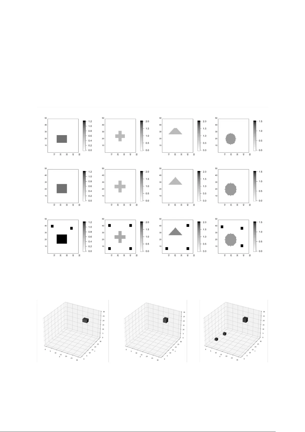
Ba y esian Scalar-on-T ensor Quan tile Regression for Longitudinal Data on Alzheimer’s Disease Rongk e Lyu ∗ , Marina V ann ucci ∗ and Suprateek Kundu † Abstract As a general and robust alternativ e to traditional mean regression models, quan- tile regression av oids the assumption of normally distributed errors, making it a v ersatile c hoice when mo deling outcomes suc h as cognitive scores that typically ha ve sk ew ed distributions. Motiv ated b y an application to Alzheimer’s disease data where the aim is to explore how brain-b eha vior associations change o ver time, w e prop ose a no vel Bay esian tensor quantile regression for high-dimensional longi- tudinal imaging data. The proposed approach distinguishes betw een eﬀects that are consisten t across visits and patterns unique to eac h visit, contributing to the o verall longitudinal tra jectory . A low-rank decomp osition is employ ed on the ten- sor co eﬃcien ts which reduces dimensionalit y and preserv es spatial conﬁgurations of the imaging vo xels. W e incorp orate multiw ay shrink age priors to model the visit- in v ariant tensor co eﬃcien ts and v ariable selection priors on the tensor margins of the visit-sp eciﬁc eﬀects. F or p osterior inference, we develop a computationally ef- ﬁcien t Marko v chain Monte Carlo sampling algorithm. Sim ulation studies reveal signiﬁcan t impro v ements in parameter estimation, feature selection, and predic- tion p erformance when compared with existing approac hes. In the analysis of the Alzheimer’s disease data, the ﬂexibility of our mo deling approach brings new in- sigh ts as it provides a fuller picture of the relationship b et ween the imaging v o xels and the quantile distributions of the cognitive scores. Keyw ords: Low-rank Decomp osition; Spatial F unctional Predictor; Shrink age Priors; Neuroimaging Data; Robust Mo deling ∗ Departmen t of Statistics, Rice Univ ersity , Houston, TX, USA † Departmen t of Biostatistics, MD Anderson Cancer Center, Houston, TX, USA 1 1 In tro duction Alzheimer’s disease (AD) is a neuro degenerativ e disease of the brain that aﬀects an es- timated 7 million Americans aged 65 or older, with an estimated public health cost of around 360 billion. This num b er could grow to 13.8 million by 2060 barring the devel- opmen t of medical breakthroughs (Better, 2023). Neuroimaging studies ha ve emerged as an in v aluable to ol for identifying individuals susceptible to neurological and clinical con- ditions. By discerning subtle abnormalities in brain structure and function, researchers can no w predict the risk of men tal disorders (including AD and dementia) with greater precision. In particular, structural neuroimaging studies in volving magnetic resonance imaging (MRI), hav e revealed the in tricate patterns of atrophy in spatially distributed brain regions in volv ed in memory and cognition, whic h is a hallmark of AD (F renzel et al., 2020). Neuroimaging features suc h as brain v olume or cortical thickness (CT) deriv ed from MRI scans can be used to provide quantitativ e assessments of structural atroph y and monitor disease progression ov er time, with CT emerging as a highly sensi- tiv e neuroimaging biomarker for AD (Du et al., 2007; W eston et al., 2016). Progression to dementia due to AD inv olves multiple path wa ys of disease pathophysiology that im- pact cognition (Jack Jr et al., 2018; Jac k et al., 2013; Jagust, 2018). Individuals who dev elop demen tia follow a tra jectory from a stage of normal cognition to Mild Cogni- tiv e Impairment (MCI) and subsequent dementia (McKhann et al., 2011; Petersen et al., 2001; Sp erling et al., 2011). There has b een very limited w ork on attempting to delineate gradual changes due to disease progression o ver visits, which is particularly critical giv en the current 2018 NIA-AA researc h framework that has transitioned to deﬁning AD as a con tinuum (Aisen et al., 2017). F or instance, there is a lack of principled statistical ap- proac hes that can map spatially distributed longitudinal CT changes in the brain surface and b orro w information across longitudinal brain images to mo del cognitive impairment. Standard neuroimaging approac hes for risk prediction typically use informative sum- mary measures or v oxel-wise analysis (Rathore et al., 2017). These approaches are useful in terms of reducing the dimensions from high-dimensional images containing tens of thousands of v oxels to a smaller subset of informative global or region-sp eciﬁc features. Ho wev er, they result in p oten tial information loss and do not resp ect the spatial in- formation in the images. Scalar-on-image regression metho ds hav e b een prop osed that carefully accoun t for the spatial conﬁguration of hundreds of thousands of v oxels, via 2 basis representations of the images. These approac hes may be considered as an extension of scalar-on-function mo dels to functional imaging data, and in volv e metho ds such as functional principal comp onen ts (Zipunniko v et al., 2011; F eng et al., 2020), as w ell as w av elet-based metho ds (W ang et al., 2014; Reiss et al., 2015; Ma et al., 2024). Sepa- rately , Mark ov random ﬁeld (MRF) metho ds ha v e b een prop osed (Lee et al., 2014; Smith and F ahrmeir, 2007). While they are based on solid theoretical foundations, MRF ap- proac hes and basis expansion metho ds typically inv olv e a large num b er of parameters to mo del high-dimensional images that may induce the curse of dimensionalit y . T o b ypass these issues, scalar-on-tensor mo dels hav e seen an increasing p opularit y for mo deling im- age data (Guhaniy ogi et al., 2017; Zhou et al., 2013; Liu et al., 2023; Lyu et al., 2024). T ensor-based approaches are attractiv e since they result in massive dimension reduction and they simultaneously preserve the spatial information in the images (Kundu et al., 2023). The bulk of tensor mo deling literature, including the ab o ve approaches, fo cuses on mean regression mo dels in volving normally distributed errors. Ho wev er, the Gaussianit y assumptions ma y not hold when mo deling complex outcomes such as cognitiv e scores that t ypically ha v e skew ed distributions, see Figure 4 for an illustration of the outcome data used in our application. Additionally , when mo deling cognitiv e outcomes as in our motiv ating application, it may b e more meaningful to inv estigate the eﬀect of imaging co v ariates on the outcome distribution, rather than solely fo cusing on the mean. One can ac hieve this type of analysis via quantile regression (Ko enk er and Bassett Jr, 1978; Ko enk er and Hallo c k, 2001), which oﬀers a more robust approac h than mean regression b y handling outliers and accommo dating deviations from normality . Bay esian quantile regression approaches, in particular, hav e seen a ric h developmen t ov er the past couple of decades. Y u and Moy eed (2001) prop osed a Ba yesian approach to quan tile regression that uses asymmetric Laplace Distribution (ALD) priors. Dunson and T aylor (2005) pro- p osed a substitution lik eliho o d method to approximate Ba y esian inferences on diﬀerences in quan tiles and F eng et al. (2015) prop osed a Bay esian metho d that uses linear inter- p olation of the quantiles to appro ximate the likelihoo d. Among nonparametric Bay esian approac hes, Kottas and Krnja ji´ c (2009) prop osed a semiparametric approach based on Diric hlet pro cess mixture mo dels. Kottas et al. (2007) prop osed an additive quantile regression framework with Gaussian pro cess priors, that w as later extended to allow 3 for partially observed resp onses in a T obit quan tile regression framework b y T addy and Kottas (2010). Reic h and Smith (2013) prop osed a Ba yesian quantile regression mo del for censored data. Additionally , T okdar and Kadane (2012) prop osed a semi-parametric approac h for sim ultaneously mo deling multiple quantiles, and Das and Ghosal (2018) dev elop ed a non-parametric approach for complete and grid data. Recen tly , Das et al. (2023) prop osed a Bay esian hierarchical quantile regression that simultaneously mo dels the hierarchical relationship of multi-lev el cov ariates. In spite of the rich developmen t on quantile regression approaches, the literature on mo dels inv olving high-dimensional functional cov ariates is somewhat limited. Cardot et al. (2005) prop osed a scalar-on-function quantile regression problem using a spline estimator to minimize a p enalt y term, while Kato (2012) considered the principal com- p onen t analysis metho d in a similar setting. Zhang et al. (2022) incorp orated imaging data in to the quantile regression as a functional resp onse based on a function-on-scalar framew ork. W ang et al. (2023) introduced the quan tile latent-on-image regression with a tw o-stage mo del, using functional principal comp onen ts of the images as predictors. Recen t work has lev eraged tensor-mo deling approaches to tackle high dimensionalit y of spatially distributed imaging features under a quantile regression framework. Lu et al. (2020) ﬁrst studied scalar on tensor quan tile regression mo dels based on T uc ker decom- p osition and used regularization via L 1 p enalties, while Li and Zhang (2021) prop osed a tensor quantile regression mo del with a generalized LASSO p enalt y based on CANDE- COMP/P ARAF A C (CP) decomp ositions. W ei et al. (2023) prop osed a Bay esian tensor resp onse quan tile regression to in vestigate the asso ciation b et ween fMRI resting-state functional connectivity and PTSD symptom severit y and Liu et al. (2024) developed a scalar-on-image tensor quan tile regression based on tensor train (TT) decomp osition with a generalized lasso p enalty . In con trast to the ab o ve approaches that fo cused on cross-sectional imaging data, Ke et al. (2023) prop osed a t w o-stage estimation proce- dure for linear tensor quan tile regression inv olving longitudinal tensor-v alued data. They used generalized estimation equations for estimation, follow ed b y k ernel smo othing to construct smo oth tensor co eﬃcien ts in order to tac kle high-dimensional cov ariates. As for Bay esian approaches, Reich et al. (2011) and Reic h (2012) considered spatiotemp oral quan tile regression mo dels where each spatial lo cation has its own quantile function that ev olves ov er time and smo othed spatially via Gaussian pro cess priors. W ang and Song 4 (2024) dev elop ed a Ba y esian nonparametric scalar-on-image quantile regression model based on Gaussian pro cesses to analyze the asso ciation b et w een cognitiv e decline and clinical v ariables. While the existing Bay esian approac hes for quan tile regression describ ed abov e are at- tractiv e in providing uncertaint y quantiﬁcation and p erforming inference, they often rely on Gaussian pro cess priors that may not b e scalable to high-dimensional images contain- ing tens of thousands of spatially distributed v oxels. Moreo ver, approaches for Bay esian quan tile regression approaches to map longitudinal neuroimaging c hanges are limited. In one of the ﬁrst such attempts, w e develop a nov el Bay esian tensor quan tile regression for high-dimensional longitudinal brain imaging data that uses tensor representations to mo del the longitudinal imaging co eﬃcien ts in order to tackle high-dimensionality . Our goal is to estimate the longitudinal tra jectory of brain-b eha vior asso ciations and to infer signiﬁcan t neuroimaging biomark ers by po oling information across visits, while accurately predicting diﬀerent quantiles of the outcome distribution. A key asp ect of our prop osed approac h is the ability to diﬀerentiate b et w een common asso ciations across visits from visit-sp eciﬁc patterns contributing to longitudinal tra jectories. This is made p ossible via a visit-inv arian t tensor co eﬃcient that is learn t by systematically p ooling information across visits, and additionally incorporating separate visit-sp eciﬁc tensor coeﬃcients. F ur- thermore, a scalar random intercept term mo dels the within-sub ject longitudinal dep en- dencies in the outcome, while the similarit y across visits is captured via the visit-in v arian t tensor co eﬃcien t term. W e assume a low-rank P ARAF A C decomp osition on the tensor co eﬃcien ts, preserving the spatial conﬁguration of imaging vo xels while addressing the c hallenges p osed b y the high dimensionalit y . W e incorp orate m ultiw ay shrink age priors (Guhaniy ogi et al., 2017) to mo del the visit-inv arian t tensor co eﬃcien ts. W e imp ose a spik e and slab prior on the tensor margins for the visit-sp eciﬁc eﬀects, which encourages sparsit y and controls the degree of c hanges across visits from b ecoming exceedingly large. W e dev elop an MCMC algorithm for p osterior inference that com bines Gibbs sampling steps based on lo cation-scale mixture represen tations with v ariable selection sto chastic searc h algorithms. Our contributions are motiv ated b y ADNI-1 neuroimaging study , where the goal is to mo del quantiles of the cognitive score distribution based on T1-weigh ted MRI scans across longitudinal visits, and infer neuroimaging biomarkers driving cognitive deﬁcits. 5 Our analysis displays considerably impro ved prediction accuracy across v arious quantile lev els consisten tly for b oth AD and MCI cohorts. Our results reveal sparse asso ciations b et ween the imaging vo xels and the median cognitiv e scores, but more pronounced asso- ciations with tails of the distributions of the cognitive scores. F urthermore, our approac h allo ws the iden tiﬁcation of brain regions that are signiﬁcan tly asso ciated with adv anced cognitiv e impairment, which can serv e as promising neuroimaging biomarkers. F or in- stance, our analysis identiﬁed several gyral regions that show ed signiﬁcant asso ciations with the 80-th quantile of the ADAS cognitiv e score (implying adv anced cognitive im- pairmen t) but limited signiﬁcant asso ciations with the median or 20-th quantiles of the AD AS score distribution (indicating a more normal cognitive functioning). With resp ect to existing Ba yesian quan tile metho ds for functional cov ariates based on Gaussian pro- cesses, our analysis provides a more comprehensive understanding of disease progression and iden tiﬁcation of neuroimaging biomarkers, by ev aluating the longitudinal tra jectory of neuroimaging eﬀects on v arious quan tiles of the cognitive score distribution. Addi- tionally , w e p erform extensiv e sim ulation studies that show signiﬁcant improv emen ts in parameter estimation, feature selection, and prediction accuracy when compared to v ar- ious comp eting metho ds. The rest of the paper is organized as follows: In Section 2, we describ e the prop osed tensor quantile regression mo del for longitudinal data and develop an MCMC algorithm for p osterior inference. W e also discuss m ultiplicit y adjustmen ts to control the Type 1 error. In Section 3 we in vestigate the mo del p erformances through comprehensive sim ulation studies. In Section 4 w e discuss our results from the data analysis using the ADNI dataset. 2 Metho ds In its simplest form, a quan tile regression mo del can b e obtained from OLS regression as Q q ( y i ) = x T i β + ϵ q , i = 1 , . . . , n, (1) with q denoting the quantile lev el of in terest and ϵ q the error term that is distributed suc h that it is zero at the q -th quan tile. Our goal is to extend the classical Ba yesian quan tile regression framework in (1) to the case of longitudinal studies in volving high- 6 dimensional spatial images as cov ariates, utilizing tensor-based metho ds to address the curse of dimensionality and incorp orate spatial information in the mo del framework. 2.1 Ba y esian T ensor Quan tile Regression for Longitudinal Data W e hav e av ailable longitudinal MRI data on n sub jects, each of whom has a maximum of T visits. The i th sample ( i = 1 , . . . , n ) has T i ≤ T visits, where the visit index b elongs to the set { 1 , 2 , . . . , T } , with the understanding that sub jects with missing visits will ha ve data collected on a subset of visit indices { 1 , 2 , . . . , T } . Let T it denote the time from baseline at the t -th visit for the i th individual, denote X it as the brain image for the i th sub ject at the t th visit, and denote the corresp onding scalar outcome v ariable as y it . F urther, let z i = ( z i 1 , . . . , z ip ) denote the v ector of time-in v ariant non-imaging cov ariates, for the i th sub ject. The prop osed approac h assumes regular visit times across samples, that is consisten t with the design of ADNI study (Jack et al., 2008) used for our data analysis. Ho wev er, our approac h can accommo date missing visits resulting in v arying n umber of visits across samples, as elab orated in the sequel. W e write our prop osed Ba yesian Longitudinal T ensor Quan tile Regression (BL TQR) as: Q q ( y i,t ) = b 0 + b 0 i + b 1 ∗ T it + z T i η + ⟨X it , B 0 ⟩ + ⟨X it , B t ⟩ + ϵ q it , (2) where q is the quan tile lev el, b 0 and b 1 represen t the group-lev el in tercept and slop e, and b 0 i is the sub ject-sp eciﬁc intercept con tributing to the v ariations in the longitudinal patterns across sub jects. The eﬀect of the brain image X it is expressed as the sum of a visit-inv ariant eﬀect ( B 0 ) and a visit-sp eciﬁc eﬀect ( B t ), with b oth B 0 and B t tensors of dimensions p 1 × p 2 , and with ⟨· , ·⟩ in mo del (2) denoting the tensor inner product. The longitudinal tra jectories are accounted for via visit-sp eciﬁc images X it , as well as the slop e term. While the mo del can b e easily generalized to include additional sub ject- sp eciﬁc random slop e terms, we found the mo del (2) to w ork suﬃciently well in practical applications including the ADNI analysis in Section 4. In addition, w e note that the mo del is naturally designed to handle missing visits. In particular, the prop osed mo del in volv es t wo types of co eﬃcients: (a) a time-in v ariant parameter B 0 and other scalar parameters that do not dep end on the visit index and are estimated by com bining information across 7 all visits and samples; and (b) time-sp eciﬁc parameters B t that is estimated b y p o oling information across all samples with data at the t -th visit, whic h is comparable across samples under the assumption of regular visit timings. F or b oth (a) and (b) missing visits for a subset of samples do not alter the mo del implementation in an y wa y . W e complete our quan tile regression mo del by assuming an asymmetric Laplace dis- tribution (ALD) on the error term in equation (2) as f ( ϵ q it | σ, q ) = q (1 − q ) σ exp  − ρ  ϵ q it σ  . Kozumi and Koba yashi (2011) show ed that ALD can b e represen ted as a lo cation-scale mixture of normal distributions where the mixing distribution follows an exp onen tial distribution. Th us, equation (2) can b e rewritten as Q q ( y i,t ) = b 0 + b 0 i + b 1 ∗ T it + z T i η + ⟨X it , B 0 ⟩ + ⟨X it , B t ⟩ (3) + θ ν it + ρ √ σ ν it u it , with ν it = σ m it , θ = 1 − 2 q q (1 − q ) , and ρ 2 = 2 q (1 − q ) , and where m it follo ws a standard exponential distribution and u it a standard normal distribution. Our prop osed mo del emplo ys a tensor-based representation of the imaging data. A tensor is a m ulti-dimensional array , with the order b eing the num b er of its dimensions. F or example, a one-w a y or ﬁrst-order tensor is a v ector, and a second-order tensor is a matrix. Mathematically , a N -dimensional tensor X can b e expressed as X ∈ R I 1 × I 2 ×···× I N , where I n indicates the size of the tensor in the n -th dimension. T ensors ha ve gained recognition as a modeling to ol for neuroimaging data as they can ac hiev e dimension reduction via low rank decomp ositions on the mo del parameters, while preserving the spatial information in the image. Here we emplo y tensor decomp ositions for the visit-inv ariant eﬀect ( B 0 ) and the visit- sp eciﬁc tensor eﬀects ( B t ). T ensor decomposition is a mathematical tec hnique that breaks do wn a high-dimensional tensor in to a com bination of lo wer-dimensional factors. One t yp e of tensor decomp osition is the T uck er decomp osition (Kolda and Bader, 2009), whic h decomp oses a tensor into a core tensor and a set of matrices, one along each mo de. Another commonly used tec hnique is the P ARAF AC decomp osition, a sp ecial case of the T uck er decomp osition, where the core tensor Λ is restricted to b e diagonal. The 8 rank- R P ARAF A C mo del expresses the high-dimensional tensor as an outer pro duce of one-dimensional tensor margins, summed ov er R channels. Here, we emplo y P ARAF A C decomp ositions that expresses the visit-inv ariant eﬀect ( B 0 ) and the visit-sp eciﬁc tensor eﬀects ( B t ) as B 0 = R X r =1 β ( r ) 01 ◦ · · · ◦ β ( r ) 0 D , and B t = R t X r t =1 χ ( r t ) t 1 ◦ · · · ◦ χ ( r t ) tD . (4) where β 01 , . . . , β 0 D and χ t 1 , . . . , χ tD , known as tensor margins, are vectors of length p 1 , . . . , p D , and where β 01 ◦ · · · ◦ β 0 D and χ t 1 ◦ · · · ◦ χ tD are a D-wa y outer pro duct of dimension p 1 × p 2 × . . . × p D . F or our neuroimaging applications, D = 2 for 2-dimensional slices and D = 3 for three-dimensional images. The assumed rank of the visit-sp eciﬁc eﬀect ( R t ) is allo wed to be diﬀeren t from the assumed rank of the visit-in v arian t eﬀect ( R ) to ensure that b oth eﬀects are b eing mo deled and optimized separately . The appropriate tensor rank v ary dep ending on the sp eciﬁc application con text and can b e c hosen using a go o dness-of-ﬁt approac h (Guhaniyogi et al., 2017; Liu et al., 2023). W e note that, ev en though the tensor margins can only b e uniquely iden tiﬁed up to a p erm utation and a m ultiplicative constant, the tensor pro duct is fully identiﬁable, whic h suﬃces for our primary ob jective of estimating co eﬃcien ts. The P ARAF A C decomp osition dramatically reduces the num b er of co eﬃcien ts from p 1 × . . . × p D to R ( p 1 + . . . + p D ), which grows linearly with the tensor rank R and results in signiﬁcant dimension reduction. Prior to applying the tensor mo del, the image’s v oxels are mapp ed on to a grid, making them more suitable for a tensor-based approach. This mapping conserv es the spatial arrangemen ts of the vo xels. While the grid mapping migh t not preserv e exact spatial distances b et ween v o xels, this has limited impact in our exp erience, since it can still capture correlations b et ween neigh b oring elements in the tensor margins. Moreov er, the tensor construction has the adv an tageous ability to estimate vo xel-sp eciﬁc co eﬃcients b y lev eraging information from neigh b oring vo xels through the estimation of tensor margins with their inheren t lo w-rank structure. This feature results in a type of spatial smoothing and results in brain maps that are more consisten t and robust to missing vo xels and image noise. F or more details on the c haracteristics of Ba y esian tensor mo dels, we refer readers to Kundu et al. (2023). 9 2.2 Prior mo del Let’s start with the prior choice for the tensor co eﬃcients. F or the tensor margins of the visit-unsp eciﬁc tensor B 0 , we adopt the multiw a y Dirichlet generalized double Pareto (M- DGDP) prior from Guhaniy ogi et al. (2017), whic h shrinks small coeﬃcients to w ards zero while minimizing shrink age of large co eﬃcien ts. Let W j r = Diag( w j r, 1 , . . . , w j r,p j ), with w j r,k , for k = 1 , . . . , p j , elemen t-wise margin-sp eciﬁc scale parameters. The M-DGDP prior can b e expressed in hierarc hical form as: β ( r ) 0 j ∼ N (0 , ( ϕ r τ ) W j r ) , w j r,k ∼ Exp  λ 2 j r / 2  , λ j r ∼ Ga ( a λ , b λ ) , ( ϕ 1 , . . . , ϕ R ) ∼ D ir ichlet ( α 1 , . . . , α R ) , (5) τ ∼ Ga ( a τ , b τ ) . The parameter τ is a global scale parameter, while parameters Φ = ( ϕ 1 , . . . , ϕ R ) encourage shrink age to low er ranks in the assumed P ARAF AC decomp osition. Marginalizing out the scale parameters w j r,k , one obtain β ( r ) j,k | λ j r , ϕ r , τ iid ∼ DE  λ j r / p ϕ r τ  , 1 ≤ k ≤ p j , (6) that is, prior (5) induces a GDP prior on the individual margin co eﬃcien ts whic h in turn has the form of an adaptive Lasso p enalt y (Armagan et al., 2013). F or the visit-sp eciﬁc eﬀects B t , we adapt a form of the spike-and-slab prior to our set- ting, as w e exp ect these signals to b e sparse. V arious spik e-and-slab priors ha ve been pro- p osed in the ﬁeld of Ba yesian statistics, see T adesse and V annucci (2021) for an ov erview on the diﬀerent approaches. These emplo y hierarchical prior structures and sto c hastic searc h MCMC metho ds to iden tify mo dels with a high posterior probabilit y of o ccurrence. As the n um b er of co v ariates increases, the task of determine the c hoice of priors b ecomes more c hallenging, since in man y circumstances the high-frequency mo del is not the opti- mal predictive mo del (Barbieri and Berger, 2004). Here we adopt the prior construction of Ish waran and Rao (2003, 2005), who emplo yed a mo diﬁed rescaled spik e and slab mo dels using contin uous bimo dal priors for the v ariance hyperparameters, and whic h has prov ed to b e suitable for scenarios with large num b er of cov ariates. Ro ˇ ck ov´ a and George (2014) 10 prop osed a similar formulation using a discrete spike-and-slab mo del for the cov ariance parameters and emplo ying the EM algorithm to rapidly identiﬁes promising submodels. Let W χ tj r t = diag ( w χ tj r t , 1 , . . . , w χ tj r t ,p j ). W e imp ose spik e-and-slab priors on the v ariance terms of the tensor margins of B t as χ ( r t ) tj ∼ N (0 , ( ϕ χ tr t τ χ t ) W χ tj r t ) w χ tj r t ,k | π tj r t ,k , λ tj r t ∼ (1 − π tj r t ,k ) δ ν + π tj r t ,k E xp ( λ 2 tj r t ) π tj r t ,k ∼ B er n ( ζ tj r t ) , ζ tj r t ∼ B eta ( a ζ , b ζ ) , ( ϕ tr t , . . . , ϕ tR t ) ∼ D irichl et ( α 1 , . . . , α R ) , τ χ t ∼ Ga ( a τ , b τ ) , λ tj r t ∼ Ga ( a λ , b λ ) . (7) with δ ν denoting a p oin t mass at ν . In our construction, π tj r t ,k = 1 corresp onds to large v ariances, encouraging large w tj r t ,k v alues. With resp ect to the more commonly used spik e-and-slab priors on individual regression co eﬃcien ts, this construction has the com- putational adv an tage of retaining the blo c k up date for the tensor margins χ ( r t ) tj , whic h drastically optimizes the computational cost of our MCMC sampling algorithm, as de- scrib ed in section 2.3. T o preserve the positive semi-deﬁniteness of the cov ariance matrix, w e set the spik e at a small p ositiv e v alue that is nonzero ( ν = 10 − 4 in the applications of this pap er). Finally , w e complete the prior sp eciﬁcation by assuming an In verse Gamma distribution on σ 2 , and standard Gaussian priors on b 0 , b 1 , b 0 i , and η . 2.3 MCMC Algorithm F or p osterior inference, we emplo y a Marko v Chain Monte Carlo (MCMC) algorithm that com bines Gibbs sampling steps based on lo cation-scale mixture represen tation of the asymmetric Laplace distribution (Kozumi and Koba y ashi, 2011), and v ariable selection sto c hastic searc h algorithms that use add-delete-swap mov es (Savitsky et al., 2011). The algorithm is summarized b elo w and the full details of the up dates are pro vided in the Supplemen tary Material. A generic iteration of the MCMC algorithm comprises of the follo wing up dates: • Dra w σ from the full conditional 11 p ( σ | y , B 0 , B t , ν it , b 0 , b 0 i , b 1 , η ) ∼ IG( a/ 2 , b/ 2) , with a = n 0 + 3 nT and b = 1 ρ 2 P T t =1 P n i =1 ( y it − µ it ) 2 ν it + s 0 + 2 P T t =1 P n i =1 ν it , and where µ it = b 0 + b 0 i + b 1 ∗ T it + z T i η + ⟨X it , B 0 ⟩ + ⟨X it , B t ⟩ + θ ν it . • Dra w ν it from the full conditional p ( ν it | y it , B 0 , B t , σ, b 0 , b 0 i , b 1 , η ) ∼ GIG( 1 2 , δ it , γ it ) , with δ 2 it = ˜ y 2 it ρ 2 σ , γ 2 it = θ 2 ρ 2 σ + 2 σ , and ˜ y it = y it − b 0 − b 0 i − b 1 ∗ T it − z T i η − ⟨X it , B 0 ⟩ −⟨X it , B t ⟩ . • Dra w b 0 from the full conditional p ( b 0 | y , B 0 , B t , σ, ν , b 0 i , b 1 , η ) ∼ N ( µ b 0 , σ 2 b 0 ) , with σ 2 b 0 = ( P T t =1 P n i =1 1 ρ 2 σ ν it ) − 1 , µ b 0 = σ 2 b 0 ( P T t =1 P n i =1 ˜ y it ρ 2 σ ν it ), and ˜ y it = y it − b 0 i − b 1 ∗ T it − z T i η − ⟨X it , B 0 ⟩ − ⟨X it , B t ⟩ − θ ν it . • Dra w b 0 i from the full conditional p ( b 0 i | y i , B 0 , B t , σ, ν it , b 0 , b 1 , η ) ∼ N ( µ 0 i , σ 2 0 i ) , with σ 2 0 i = ( P T t =1 1 ρ 2 σ ν it + 1) − 1 ; µ 0 i = σ 2 0 i P T t =1 ˜ y it ρ 2 σ ν it , and ˜ y it = y it − b 0 − b 1 ∗ T it − z T i η − ⟨X it , B 0 ⟩ − ⟨X it , B t ⟩ − θ ν it . • Dra w b 1 from the full conditional p ( b 1 | y , B 0 , B t , σ, ν it , b 0 , b 0 i , η ) = N ( µ b 1 , σ 2 b 1 ) , with σ 2 b 1 = ( P T t =1 P n i =1 T 2 it ρ 2 σ ν it + 1) − 1 ; µ b 1 = σ 2 b 1 ( P T t =1 P n i =1 ˜ y it T it ρ 2 σ ν it ), and ˜ y it = y it − b 0 − b 0 i − z T i η − ⟨X it , B 0 ⟩ − ⟨X it , B t ⟩ − θ ν it . 12 • Up date [ α, Φ , τ | B 0 , W ] comp ositionally as [ α | B 0 , W ][Φ , τ | α, B 0 , W ], as de- scrib ed in Guhaniyogi et al. (2017). • Sample { ( β ( r ) 0 j , w j r , λ j r ); 1 ≤ j ≤ D , 1 ≤ r ≤ R } using a bac k-ﬁtting pro cedure to pro duce a sequence of dra ws from the margin-level conditional distributions across comp onen ts. F or r = 1 , ..., R and j = 1 , ..., D , sample from the conditional distribu- tion h β ( r ) 0 j , w j r , λ j r  | β ( r ) 0 , − j , B 0 , − r , y , Φ , τ , η , σ, ν i , where β ( r ) 0 , − j = n β ( r ) 0 l , l  = j o and B 0 , − r = B \B 0 r , as: (a) Dra w h w j r , λ j r | β ( r ) 0 j , ϕ r , τ i = h w j r | λ j r , β ( r ) 0 j , ϕ r , τ i h λ j r | β ( r ) 0 j , ϕ r , τ i . 1. Dra w λ j r ∼ Ga  a λ + p j , b λ +    β ( r ) 0 j    1 / √ ϕ r τ  ; 2. Dra w w j r,k ∼ GIG  1 2 , λ 2 j r , β 2( r ) 0 j,k / ( ϕ r τ )  indep enden tly for 1 ≤ k ≤ p j . (b) Dra w β ( r ) 0 j ∼ N ( µ β 0 j r , Σ β 0 j r ). See full expressions of µ β 0 j r and Σ β 0 j r ) in the Sup- plemen tary Material. • Up date [ α χ t , Φ χ tr t , τ χ t | B t , W χ tj r t ] comp ositionally as [ α χ t | B t , W χ tj r t ][Φ χ tr t , τ χ t | α χ t , B t , W χ tj r t ], as describ ed in Guhaniy ogi et al. (2017). • Join tly up date ( π ( r t ) tj , w χ tj r t ). This is a joint Metrop olis-Hastings step. W e use the add/delete/swap metho d to prop ose a new candidate π ∗ tj r t ,k , and up date the added/deleted or sw app ed v o xels w χ tj r t ) based on the prop osed π ∗ tj r t ,k . The pro- p osed candidate is join tly accepted or rejected. See Supplemen tary Material for full details of the acceptance probability . • Sample { ( χ ( r t ) tj , λ tj r t ); 1 ≤ j ≤ D , 1 ≤ r t ≤ R t } using a back-ﬁtting pro cedure to pro duce a sequence of dra ws from the margin-level conditional distributions across comp onen ts. F or r t = 1 , ..., R t and j = 1 , ..., D , sample from the conditional distribution h χ ( r t ) tj , λ tj r t )  | χ ( r t ) t, − j , B t, − r t , y t , Φ χ t , τ χ t , η , σ, ν i . as: 13 – Dra w λ tj r t ∼ Ga  a λ + p j , b λ +    χ ( r ) tj    1 / q ϕ χ t,r t τ χ t  ; – Dra w χ ( r t ) tj ∼ N ( µ χ tj r t , Σ χ tj r t ). See full expressions of µ χ tj r t , and Σ χ tj r t in the Sup- plemen tary Material. • Dra w ζ tj r t from p ( ζ tj r t | π tj r t ) ∼ B eta ( α, β ) , with α = a ζ + P p j k =1 ( π ( r t ) tj,k and β = b ζ + P p j k =1 (1 − π ( r t ) tj,k . • Dra w η from p ( η | y , B 0 , B t , σ, ν , b 0 , b 0 i , b 1 ) ∼ N ( µ η , Σ η ) , with Σ − 1 η = P T t =1 z T 1 /ν t z ρ 2 σ + Σ − 1 0 η , µ η = Σ η ( P T t =1 z T ˜ y ρ 2 σ ν t ), and ˜ y it = y it − b 0 − b 0 i − b 1 ∗ T it − ⟨X it , B 0 l ⟩ − ⟨X it , B t ⟩ − θ ν it . 2.4 P osterior Inference Giv en the MCMC output, we obtain estimates of the cell-lev el tensor eﬀects for eac h longitudinal visit and achiev e feature selection as follows. In our mo del formulation, the tensor eﬀect p er visit is captured b y b oth the esti- mated visit-sp eciﬁc and visit-unsp eciﬁc eﬀects as ( ˆ B 0 + ˆ B t ). Let θ tj , j = 1 , . . . , J b e the vectorized tensor co eﬃcien ts at visit t , with J = Q D k =1 p k the total num b er of cells in the image X t . Supp ose K p osterior samples across J elements of a tensor-v alued co eﬃcien t denoted as n Γ k =  Γ k ( θ 1 ) , . . . , Γ k ( θ J )  ′ : k = 1 , . . . , K o w ere obtained after burn-in. W e obtain the signiﬁcan t co eﬃcient estimates with multiplicit y adjustments. Multiplicit y adjustmen t is a widely-used technique to control the increased risk of Type I errors, i.e., the false discov ery rate. Sp eciﬁcally , we used the “Mdev” metho d, whic h relies on simultaneous credible bands, introduced in (Crainiceanu et al., 2007) and later adopted b y Hua et al. (2015) and Kundu et al. (2023). Giv en the p osterior sample curv e \ Γ ( θ j ) and the p oin t-wise α / 2 and 1 − α / 2 quan tiles ζ α/ 2 ( θ j ) and ζ 1 − α/ 2 ( θ j ), the Mdev method computes the maximal deviations ζ ∗ α/ 2 = max j =1 ,...,J  \ Γ ( θ j ) − ζ α/ 2 ( θ j )  and ζ ∗ 1 − α/ 2 = max j =1 ,...,J  ζ 1 − α/ 2 ( θ j ) − \ Γ ( θ j )  . The credible bands for each vo xel are 14 obtained as h \ Γ ( θ j ) − ζ ∗ α/ 2 , \ Γ ( θ j ) + ζ ∗ 1 − α/ 2 i , where the v o xel θ j is considered signiﬁcan t if the corresp onding credible in terv al do es not con tain zero. 3 Sim ulation Study In this section, w e assess mo del p erformance via several distinct sim ulated scenarios, where w e consider b oth visit-v arying and visit-inv arian t eﬀects, and compare results with comp eting metho ds. 3.1 Data Generation W e generate the data under several scenarios. T o assess the prop osed metho d’s ability to retain spatial information of the images, while po oling information across spatially distributed v o xels and longitudinal visits, w e generate data from 3 visits with the v arying signal shap es. F or each visit, the signal image is generated with dimension 48 b y 48 for Scenarios 1-4, and from a 30 × 30 × 30 3-D image in Scenario 5. F or eac h scenario, we v aried the size and magnitudes of these signals while keeping the signal shap e constan t across visits. In addition, we included some sparse signals with magnitudes ranging from 1.2 to 2 at the last visit for all scenarios. Notably , the co eﬃcien t signal shap es used for data generation did not follow the lo w rank P ARAF A C decomp osition that is implicit under our mo deling construction. • Scenario 1 : Rectangular signals v arying in lo cations and magnitudes, with addi- tional sparse signals in the last visit. • Scenario 2 : Cross-shap ed signals v arying in lo cations and magnitudes, with addi- tional sparse signals in the last visit. • Scenario 3 : T riangular signals v arying in lo cations and magnitudes, with addi- tional sparse signals in the last visit. • Scenario 4 : Circular signals v arying in lo cations and magnitudes, with additional sparse signals in the last visit. • Scenario 5 : Cubic 3-D shap es for 30 × 30 × 30 images v arying in lo cations and magnitudes, with additional sparse signals at the last visit. 15 Figure 1 sho ws the true longitudinal 2D tensor signals for four scenarios. F or eac h setting, the tensor co v ariates X t w ere generated from the standard normal distribution N (0 , 1), and the random error ϵ t w as generated from ALD (0 , σ = 1 , q ), with the quantile lev el q c hosen to b e 0.2, 0.5, and 0.8. F or eac h simulation, w e generate 250 samples p er visit for training, and addition 50 test samples were generated for ev aluating out-of-sample prediction. Figure 1: Sim ulated signals for scenarios 1-4, as describ ed in the text. Each column represen ts one scenario, with rows 1-3 represen ting the longitudinal visits. Figure 2: Sim ulated signals for 3D setup. F rom left to righ t: visit 1( with magnitude 1), visit 2( with magnitude 1), and visit 3( with magnitude 1.5). 16 3.2 P arameter Settings W e use the default v alues suggested b y Guhaniyogi et al. (2017) for the prior hyper- parameters of the Ba yesian tensor regression mo del. Sp eciﬁcally , h yp erparameter of the Diric hlet comp onen t ( α 1 , . . . , α R ) = α = (1 /R, ..., 1 /R ), a λ = 3, b λ = 2 D √ a λ , a τ = P R i =1 α i , and b τ = αR (1 /D ) are set as defaulted v alues to con trol the cell-level v ariance on tensor B . When choosing suitable v alues of the prior h yp erparameters, for the m ultiw ay shrink age prior w e set the parameters of the h yp erprior on the global scale τ to a τ = 1 and b τ = αR (1 /D ) , where R is the rank in the assumed P ARAF A C decomp osition, and set α 1 = . . . = α R = 1 /R . F or the common rate parameter λ j r , w e set a λ = 3 and b λ = 2 D √ a λ . F or the spike-and-slab prior, we set the hyperparameters of the Bernoulli probabilit y parameter δ tj r t to b e a = 1 and b = 1. In order to decide the rank of the ﬁtted mo del, we ﬁt the prop osed mo del using ranks 2-4 and choose the rank that minimized the Deviance Information Criterion (DIC) scores. DIC measures the go o dness-of-ﬁt while adjusting for mo del complexity . When ﬁtting our mo del, we ran 7000 iterations for each MCMC c hain with 2500 burnins. 3.3 P erformance Metrics P erformance metrics were selected to assess estimation accuracy and feature selection p erformance of the cell-level tensor eﬀects for each longitudinal visit and to ev aluate the prediction accuracy of the quantile estimates. W e used the following metrics to assess p oin t estimation p erformance: (i) Relativ e error of θ t , denoted as RE ( θ t ) = P J j =1 | ˆ θ tj − θ tj | P J j =1 | θ tj | , that measures the scaled absolute deviations b et ween the true and estimated parameters, with ˆ θ tj and θ tj the estimated and true co eﬃcien ts, resp ectiv ely . W e note that the v alues of relative error can b e larger than 1, since the discrepancy b et ween estimated and true v alues of tensor cells can b e greater than zero when a large p ortion of the true v alues is exactly 0. (ii) Ro ot-mean-square error of θ t , denoted as R M S E ( θ t ) = q P J j =1 ( ˆ θ tj − θ tj ) 2 J . (iii) correlation co eﬃcien t b etw een the true and estimated cell-level tensor co eﬃcien ts. F or feature selection, p erformances were ev aluated b y the following metrics: 17 (i) Sensitivit y = T P T P + F N ; (ii) Sp eciﬁcit y = T N T N + F P ; (iii) MCC = T P × T N − F P × F N √ ( T P + F P )( T P + F N )( T N + F P )( T N + F N ) , with TP the true p ositiv e, i.e. the num b er of predictions where the classiﬁer correctly predicts a p ositiv e class as p ositiv e; FP the false p ositive, i.e. the num b er of predictions where the classiﬁer incorrectly predicts a negative class as positive; TN the true negative, i.e. the num b er of predictions where the classiﬁer correctly predicts a negative class as negativ e; and FN the false negative, i.e. the num b er of predictions where the classiﬁer incorrectly classiﬁes a p ositiv e class as negative. In our scenario, the p ositive class refers to the non-zero vo xels of the tensor co eﬃcien ts, and the negative class refers to the zero v oxels of the tensor co eﬃcien ts. Finally , prediction accuracy was ev aluated based on the chec k loss function (W ang et al., 2012) as E ( l ( Y t , ˆ Q q ( Y t ))), where l ( Y it , ˆ Q q ( Y it )) =      q | Y it − ˆ Q q ( Y it ) | , Y it > ˆ Q q ( Y it ) (1 − q ) | Y it − ˆ Q q ( Y it ) | , Y it ≤ ˆ Q q ( Y it ) , and with ˆ Q q ( Y it ) the predicted q -th quantile for sub ject i at visit t . 3.4 Results In this section, we presen t the p oint estimation, feature selection, and out-of-sample prediction performance for quan tile lev el 0.5. The complete results for quan tile lev els 0.2 and 0.8 are a v ailable in Section 2 of the Supplementary Material. Figure 3 sho ws the 2D tensor estimates obtained using the prop osed metho d, on one replicate for each of the 4 scenarios. F rom this Figure, it is eviden t that the prop osed metho d is able to broadly reco v er the shap es of the 2D tensor co eﬃcien t for each visit, and an y sparse signals present in the last visit regardless of the complexity of the diﬀerent shap es. Results under the prop osed approach and comp eting metho ds for parameter estima- tion, feature selection, and prediction, a v eraged o ver 10 replicates, are rep orted in T ables 1, 2, 3, resp ectiv ely . W e consider four alternative metho ds: (i) Cross-sectional Ba yesian tensor quantile regression t yp e 1 (CsB1), obtained from our mo del by ﬁxing B 0 to b e 18 Figure 3: Estimated signals for one replicate of scenarios 1-4, as describ ed in the text. Eac h column represents one scenario, with ro ws 1-3 representing the longitudinal visits. 0 in equation (2), and placing the M-DGDP prior as in equation (5) on B t ; (ii) Cross- sectional Bay esian tensor quan tile regression type 2 (CsB2), obtained from our mo del by ﬁxing B t to b e 0 in equation (2), and placing the M-DGDP prior as in equation (5) on B 0 ; (iii) the tensor quantile regression (F req. TQR) of Li and Zhang (2021) that p erforms frequen tist cross-sectional tensor quan tile regression, with the implemen tation made pub- licly av ailable by the authors in MA TLAB; and (iv) Quantile regression (rqPen) with the lasso p enalt y from R pack age rqPen that do es not accoun t for the spatial information in the images. CsB1 essentially p erforms a cross-sectional analysis by removing the shared parameters B 0 and p erforming the analysis separately at each visit. In contrast, CsB2 p erforms another type of cross-sectional analysis by stacking data from all visits to ﬁt a common mo del without accoun ting for visit-speciﬁc diﬀerences. The tw o other frequen tist approac hes considered also ﬁt their mo del separately across diﬀerent visits. The feature selection results w ere adjusted for m ultiplicit y as describ ed in Section 2.3. It w as not p os- sible to rep ort feature selection under the frequen tist tensor quan tile regression approach as this metho d uses the Black Relaxation Algorithm to solve optimization problems and do es not inherently pro vide conﬁdence interv als. Results presented in T ables 1-2 demonstrate that the prop osed model outp erforms 19 all alternative methods in b oth co eﬃcien t estimation and feature selection, across all scenarios. In particular, the proposed approac h consisten tly has impro v ed RE and RMSE compared to all comp eting approac hes under all scenarios. The CsB1 approach is seen to ha ve a comparable estimation compared to the prop osed approach for visits 1 and 2 under Scenario 1, ho wev er the estimation is considerably p o orer for other scenarios. F or Scenario 5 including 3-D images, CsB 2 has impro ved p oin t estimation for visit 1, while the p oin t estimation is inferior relative to the prop osed approac h for other visits. Giv en that visit 3 has sparse signals, the results p oten tially suggest that the prop osed approac h is b etter suited to capture sparse signals by separating out the common eﬀects across visits and imp osing spike and slab priors for the visit-sp eciﬁc eﬀects. In terms of feature selection (as rep orted in T able 2), the prop osed approac h consisten tly has higher or comparable F-1 and MCC scores compared to alternate metho ds across all scenarios when av eraged across visits. While the CsB1 metho d sometimes has comparable F-1 and MCC scores for visits 1 and 2, its feature selection for visit 3 is considerably inferior across all settings. Moreo v er, the prop osed approac h shows consisten tly higher F-1 and MCC scores across all visits for Scenario 5 inv olving 3-D images. The sup erior p erformance under the prop osed metho d for visit 3 demonstrates the adv antages of imp osing a selection prior on the visit-sp eciﬁc tensor co eﬃcien ts for selecting signiﬁcan t cells. T able 3 presents the prediction p erformance for scenarios 1-5, a v eraged o ver 10 repli- cated datasets. The proposed model has b etter quan tile prediction accuracy , eviden t from the lo wer chec k loss v alues compared to the alternative metho ds. The discrepancy of the results b et ween the prop osed mo del and alternative metho ds also b ecomes larger as the shap e of the signals b ecomes more complex. This is evident from the increased gains in predictiv e p erformance under the prop osed approac h in other Scenarios inv olving sligh tly more complex signal shap es compared to mo dest gains in Scenario 1. Similar results hold for q = 0 . 2 , 0 . 8 , quantiles as rep orted in T ables 3,6, 11, in the Supplemen tary Material, where the prop osed approac h consistently outp erforms comp eting metho ds. W e conclude by rep orting some sp eciﬁc comments ab out the p erformances of the alternativ e approac hes. With resp ect to the prop osed metho d, the alternativ e metho ds sho w p o or out-of-sample quan tile prediction, estimation, and feature selection. CsB1 and F req. TQR rep ort notably higher prediction errors, RE, RMSE, and lo wer correlation co eﬃcien ts for the 2nd and 3rd visits across all scenarios, reﬂecting their inability to 20 T able 1: Poin t Estimation results of cell-lev el signals for the 5 scenarios p ortra y ed in Figure 1 corresp onding to q = 0 . 5. Scenarios RE RMSE Corr. Co ef. v1 v2 v3 v1 v2 v3 v1 v2 v3 1 BL TQR 0.159 0.125 0.254 0.026 0.021 0.058 0.996 0.998 0.994 CsB1 0.165 0.143 0.370 0.022 0.023 0.081 0.996 0.997 0.975 CsB2 0.656 0.493 0.546 0.101 0.068 0.160 0.938 0.971 0.912 F req. TQR 0.221 0.196 0.875 0.029 0.030 0.206 0.994 0.994 0.841 rqP en 1.080 1.082 1.026 0.277 0.306 0.390 0.165 0.172 0.047 2 BL TQR 0.291 0.217 0.258 0.031 0.024 0.060 0.991 0.995 0.992 CsB1 0.405 0.390 1.313 0.040 0.044 0.267 0.985 0.985 0.736 CsB2 1.604 1.345 0.971 0.138 0.128 0.304 0.852 0.873 0.729 F req. TQR 1.675 1.713 2.473 0.161 0.187 0.512 0.746 0.683 0.306 rqP en 0.960 1.045 1.004 0.224 0.252 0.450 0.267 0.105 0.004 3 BL TQR 0.701 0.697 1.037 0.069 0.075 0.218 0.951 0.942 0.868 CsB1 0.946 1.015 2.121 0.098 0.107 0.403 0.896 0.877 0.498 CsB2 2.393 2.327 1.380 0.173 0.175 0.325 0.780 0.774 0.674 F req. TQR 1.571 1.717 2.821 0.145 0.163 0.545 0.775 0.713 0.214 rqP en 1.061 1.276 0.997 0.216 0.227 0.445 0.295 0.320 0.128 4 BL TQR 0.524 0.382 0.447 0.094 0.087 0.115 0.945 0.962 0.952 CsB1 0.638 0.543 0.946 0.103 0.110 0.237 0.929 0.937 0.816 CsB2 1.102 0.838 0.828 0.150 0.143 0.241 0.869 0.892 0.767 F req. TQR 0.785 0.747 1.244 0.132 0.149 0.321 0.888 0.883 0.685 rqP en 1.249 1.192 0.996 0.305 0.351 0.393 0.195 0.167 0.116 5 BL TQR 1.180 0.803 1.131 0.009 0.007 0.018 0.968 0.985 0.971 CsB1 6.165 5.925 3.189 0.025 0.017 0.044 0.799 0.906 0.756 CsB2 0.880 0.997 1.605 0.006 0.007 0.022 0.984 0.978 0.946 F req. TQR 11.638 12.596 11.925 0.043 0.044 0.091 0.230 0.188 0.002 rqP en 1.119 1.016 1.245 0.037 0.036 0.065 0.021 0.000 0.147 accommo date any longitudinal c hanges that o ccurred in the signals. Similarly , the vec- torized approach rqP en rep orts p o or prediction, estimation, and feature selection. The noticeably lo w sensitivity v alues indicate that rqP en cannot select signiﬁcan t signals, leading to high prediction error, RE, RMSE, and low correlation co eﬃcien t and MCC v alues. W e notice that CsB2, diﬀeren t from all other comp eting metho ds, consistently rep orts high sensitivit y v alues across all scenarios and all visits, and reaches the highest sensitivit y v alues on the 3rd visit across all metho ds for scenarios 3 and 4, as evident in T able 2. This demonstrates the p o wer of incorp orating samples from all visits to estimate the visit-inv ariant eﬀect B 0 . How ever, CsB2 rep orts low er sp eciﬁcity , F1-score, and MCC v alues compared to the prop osed model across all scenarios, p otentially due to the lac k of 21 T able 2: F eature selection results for the 5 scenarios p ortra y ed in Figure 1 corresp onding to q = 0 . 5. Scenarios Sens. Sp ec. F1-score MCC v1 v2 v3 v1 v2 v3 v1 v2 v3 v1 v2 v3 1 BL TQR 1 1 1 1 1 1 1 1 1 1 1 1 CsB1 1 1 0.977 1 1 1 1 1 0.988 1 1 0.987 CsB2 1 1 0.88 1 0.997 0.998 0.904 0.987 0.931 0.900 0.986 0.926 rqP en 0.147 0.158 0.016 0.970 0.963 0.990 0.197 0.208 0.030 0.164 0.165 0.021 2 BL TQR 1 1 1 0.999 1 1 0.999 1 1 0.999 1 1 CsB1 1 1 0.333 1 1 0.999 1 1 0.422 1 1 0.526 CsB2 1 1 0.864 0.960 0.969 0.985 0.747 0.818 0.861 0.757 0.820 0.849 rqP en 0.120 0.076 0.005 0.995 0.985 0.999 0.199 0.117 0.009 0.246 0.109 0.042 3 BL TQR 0.997 0.967 0.647 0.997 0.997 0.999 0.968 0.956 0.777 0.967 0.953 0.788 CsB1 0.748 0.684 0.108 0.999 0.999 0.999 0.847 0.802 0.172 0.851 0.812 0.259 CsB2 0.953 0.928 0.737 0.969 0.970 0.975 0.774 0.768 0.975 0.778 0.770 0.708 rqP en 0.256 0.421 0.030 0.960 0.915 0.997 0.256 0.285 0.055 0.217 0.246 0.095 4 BL TQR 0.878 0.876 0.758 0.999 0.999 1 0.917 0.943 0.846 0.918 0.940 0.848 CsB1 0.869 0.838 0.035 0.999 0.999 1 0.904 0.904 0.064 0.901 0.900 0.173 CsB2 0.998 0.965 0.820 0.957 0.979 0.981 0.815 0.906 0.845 0.812 0.896 0.824 rqP en 0.188 0.194 0.013 0.912 0.927 0.997 0.177 0.217 0.025 0.095 0.134 0.058 5 BL TQR 1 1 0.846 1 0.999 0.999 1 0.975 0.916 1 0.961 0.919 CsB1 0.916 1 0.692 0.999 0.999 0.999 0.795 0.878 0.733 0.804 0.888 0.738 CsB2 1 1 0.802 0.999 0.998 0.999 0.975 0.967 0.908 0.972 0.947 0.899 rqP en 0.056 0.037 0.153 0.998 0.999 0.996 0.061 0.039 0.098 0.060 0.038 0.102 a visit-sp eciﬁc term. T aking into consideration that CsB2 rep orts rather p o or prediction and p oin t estimation results as evident in T ables 2 and 1, the high sensitivit y v alues result from a large num b er of falsely selected signals, and do not indicate ov erall great selection p erformance. These ﬁndings are consistent with additional feature selection results presented in T ables 2,5, 10, in Supplementary Materials. T o b etter understand the estimation and feature selection b eha vior of CsB2, we fur- ther ev aluated the p erformance under an additional scenario where the diﬀerences in the signal b et ween visits is slightly increased. The results are presented in T ables 7-8 in the Supplemen tary Material. W e ﬁnd that with increasing noise levels, the gains in feature selection (MCC) under CsB2 for scenario 4 start to diminish across the three quan tile lev- els, compared to the prop osed metho d. Therefore, we b eliev e that the prop osed metho d sho ws robust adv antages when at least a certain degree of diﬀerence exists for the s ignals at each visit. 22 T able 3: Prediction results for the 5 scenarios corresp onding to q = 0 . 5. The b est- p erformed metho ds are shown in b old. Scenarios Metho ds Visit 1 Visit 2 Visit 3 1 BL TQR 0.739 0.667 1.317 CsB TQR 1 0.736 0.660 1.714 CsB TQR 2 2.115 1.492 3.190 F req. TQR 0.783 1.594 4.709 rqP en 5.271 6.657 6.932 2 BL TQR 0.800 0.684 1.344 CsB TQR 1 0.988 0.962 4.727 CsB TQR 2 2.909 2.571 5.908 F req. TQR 3.152 3.997 10.087 rqP en 4.672 5.201 9.764 3 BL TQR 1.587 1.543 3.987 CsB TQR 1 2.020 2.092 7.248 CsB TQR 2 3.263 3.422 5.927 F req. TQR 2.814 3.480 10.673 rqP en 4.309 4.208 10.315 4 BL TQR 1.906 1.632 2.372 CsB TQR 1 2.051 2.060 5.103 CsB TQR 2 2.844 2.805 4.892 F req. TQR 2.648 3.174 6.968 rqP en 5.299 6.312 8.544 5 BL TQR 1.307 1.193 1.596 CsB TQR 1 1.353 1.370 1.831 CsB TQR 2 1.926 1.237 3.431 F req. TQR 3.188 2.833 4.990 rqP en 2.535 3.243 4.207 3.5 Computation Times and MCMC Con v ergence The computation time for tensor rank 3 corresp onding to B 0 and B t in sim ulations with 2D images was close to 8 mins per 100 iterations on a lo cal computer with 1.4 GHz Proces- sor and Memory of 8GB 2133 MHz. The corresp onding computation time for 30 × 30 × 30 3D images is ab out 85 mins p er 100 iterations for tensor rank 3. See T ables in Section 3 of the Supplementary Materials for additional details on the computation times. The computation times for 2-D and 3-D image analysis, along with our successful 3-D imple- men tation, suggest that the prop osed approac h is scalable for practical implementation in mo dern imaging studies. W e note that, even though the prop osed approach is still scalable to larger image sizes, the computation time b ecomes slow er with an increase in 23 the image size as w ell as larger tensor ranks. If needed, computation times could be impro ved on computers with greater pro cessing capability and memory , and additional sp eedups may b e p ossible using more eﬃcien t computation strategies suc h as parallelizing the up dates of the visit-sp eciﬁc B t terms. A Gewek e test (Gew ek e, 1992) was applied to diagnose the MCMC conv ergence. W e obtained the z-score from the Gewek e test for each element of the visit-unsp eciﬁc B 0 and visit-sp eciﬁc B t . In all cases (b oth in volving 2-D and 3-D images), we observed that ov er 90 p ercen t of z-scores w ere within the range of (-1.96, 1.96), indicating that c hains reached stationarit y . MCMC trace plots of the co eﬃcien ts of some of the v oxels are pro vided in the Supplementary Material. 3.6 Sensitivit y Analysis W e conducted a prior h yp erparameter sensitivit y analysis by tuning eac h h yp erparameter while ﬁxing other h yp erparameters. T able 4 displays the cell-lev el RMSE v alues of the tensor co eﬃcien t matrix B of dimension D = 2 and P ARAF A C rank- R = 3, where B is generated from Scenario 1. The ov erall results rev eal no strong sensitivity to the h yp er-parameter c hoices under the selected ranges that p oin t to a robust p erformance. Additionally , w e ev aluated the mo del p erformance as the tensor ranks were v aried, and computed the corresp onding DIC scores. The p erformance v aried sligh tly as the tensor ranks w ere changed within a reasonable range, but the p erformance was still relativ ely stable. The results are presented in T ables 12-15 of the Supplementary Materials and suggest that the model p erforms reasonably w ell across a range of tensor ranks, pro ducing stable and robust coeﬃcient estimation and feature selection performance across diﬀeren t c hoices. F urther, a low er choice of tensor ranks is often suﬃcien t to yield go o d co eﬃcien t estimation and feature selection results, for b oth 2-D and 3-D cases inv olving sparse signals. This suggests the abilit y to approximate sparse signals using low rank tensors inducing mo del parsimony . 3.7 P erformance Under Mo del Mis-sp eciﬁcation W e consider simulations with mis-sp eciﬁed settings, where the data generation used nor- mally distributed residuals instead of ALD residuals. Sp eciﬁcally , we generated data for 2-D images using co eﬃcien t signals corresp onding to Scenarios 1-4 as describ ed ab ov e, 24 but using residuals generated from a standard normal distribution N (0 , 1). The results for the q = 0 . 5 quan tile level, presented in T ables 5 and 6, clearly illustrate robust p oin t estimation and feature selection p erformance of the prop osed BL TQR approach, ev en when the residuals are normally distributed and do not follow an ALD structure. F ur- ther, the prop osed approac h results in impro vemen ts in co eﬃcient estimation o ver the t w o frequen tist metho ds that do not assume ALD errors, even under mo del mis-sp eciﬁcation. This illustrates the robustness and utility of the prop osed Bay esian mo del. T able 4: Prior hyperparameter sensitivity analysis Hyp erparameters RMSE Hyp erparameters RMSE Hyp erparameters RMSE α = 1/9 0.024 a λ = 3 0.026 a τ = 1/3 0.024 α = 1/6 0.024 a λ = 5 0.028 a τ = 1/2 0.028 α = 1/3 0.022 a λ = 7 0.024 a τ = 1 0.024 α = 3 ( − 0 . 1) 0.027 a λ = 9 0.027 a τ = 2 0.028 T able 5: P oint Estimation results of cell-lev el signals under mo del mis-sp eciﬁcation at quan tile level q = 0 . 5. Scenarios RE RMSE Corr. Co ef. v1 v2 v3 v1 v2 v3 v1 v2 v3 1 BL TQR 0.137 0.108 0.245 0.021 0.018 0.059 0.997 0.998 0.994 F req. TQR 0.330 0.170 0.927 0.043 0.026 0.205 0.986 0.995 0.837 rqP en 0.995 0.995 1.025 0.297 0.297 0.389 0.126 0.127 0.047 2 BL TQR 0.243 0.185 0.242 0.026 0.021 0.058 0.993 0.997 0.993 F req. TQR 1.670 1.700 2.608 0.157 0.170 0.537 0.760 0.734 0.310 rqP en 1.107 1.344 1.001 0.221 0.271 0.442 0.371 0.177 0.171 3 BL TQR 0.646 0.648 0.936 0.068 0.074 0.203 0.951 0.943 0.890 F req. TQR 1.414 1.339 2.799 0.137 0.147 0.503 0.802 0.773 0.340 rqP en 1 1.161 1.005 0.225 0.224 0.449 0.261 0.302 .002 4 BL TQR 0.454 0.333 0.397 0.085 0.082 0.102 0.955 0.968 0.960 F req. TQR 0.750 0.729 1.544 0.123 0.141 0.345 0.898 0.894 0.562 rqP en 1.288 1.019 1.024 0.312 0.334 0.395 0.176 0.086 0.209 4 ADNI-1 Data Analysis W e analyze longitudinal data from the Alzheimer’s Disease Neuroimaging Initiative (ADNI) 1 study collected at baseline, 6-month visit, and 12-month visit. ADNI is a large-scale, 25 T able 6: F eature selection under mo del mis-sp eciﬁcation at quantile level q = 0 . 5 Scenarios Sens. Sp ec. F1-score MCC v1 v2 v3 v1 v2 v3 v1 v2 v3 v1 v2 v3 1 BL TQR 1 1 1 1 1 1 1 1 1 1 1 1 rqP en 0.038 0.038 0.021 0.995 0.996 0.992 0.071 0.071 0.038 0.114 0.114 0.040 2 BL TQR 1 1 1 0.999 1 1 0.999 1 1 0.999 1 1 rqP en 0.384 0.296 0.095 0.942 0.912 0.991 0.322 0.228 0.162 0.281 0.169 0.196 3 BL TQR 0.997 0.962 0.748 0.995 0.996 0.999 0.954 0.950 0.775 0.953 0.948 0.793 rqP en 0.218 0.338 0.006 0.951 0.939 0.999 0.195 0.278 0.012 0.148 0.235 0.048 4 BL TQR 0.987 0.966 0.948 0.996 0.999 0.999 0.974 0.979 0.971 0.971 0.977 0.967 rqP en 0.248 0.035 0.123 0.900 0.990 0.959 0.214 0.063 0.176 0.131 0.070 0.124 longitudinal study that w as launched in 2004 to explore the progression of Alzheimer’s disease (AD) through neuroimaging and biomark er analysis (W einer et al., 2013). More detailed information for the ADNI-1 sample included for our analysis is provided in T a- ble 16 (Section 4) in the Supplemen tary Material. The revised analyses using 3D ROIs include MCI sub jects with sample sizes of 403, 311, and 321 across three visits, as well as a separate analysis for AD sub jects with sample sizes of 188, 133, and 135 across three visits. Out of these, 308 MCI and 133 AD sub jects hav e no missing visits, while other sub jects hav e one or more missing visits. 4.1 Data Source and Pre-pro cessing The T1-w eighted MRI images were pro cessed using the Adv anced Normalization T o ols (ANTs) registration pip eline (T ustison et al., 2014). This in v olved registering all images to a template to ensure consisten t normalization of brain regions across participan ts. The p opulation-based template w as created using data from 52 normal control participants in ADNI 1, originally developed by the ANTs group (T ustison et al., 2019). Notably , the ANTs pip eline includes the N4 bias correction step to address in tensit y v ariations and standardize intensit y across samples (T ustison et al., 2010). It also uses a symmet- ric diﬀeomorphic image registration algorithm for spatial normalization, aligning eac h T1 image with a brain template to enable spatial comparability (Av ants et al., 2008). Afterw ard, the pip eline used the pro cessed brain images, estimated brain masks, and template tissue lab els to p erform 6-tissue Atropos segmentation, creating tissue masks for cerebrospinal ﬂuid (CSF), gray matter (GM), white matter (WM), deep gray matter (DGM), brain stem, and cereb ellum. Finally , cortical thickness w as measured using the DiReCT algorithm. The 3D cortical thickness images of dimension 256 × 256 × 170 were 26 cropp ed to dimension 138 × 163 × 117 to remo v e the zero vo xels around the images, and then do wnsampled to a resolution of 48 × 48 × 48 using R pack age ANTsRCore . The do wnsampled cortical thickness images w ere harmonized using the ComBat approach (F ortin et al., 2018) to remov e scanner-sp eciﬁc batch eﬀects that can inﬂate v ariabilit y and cause confounding, if not accoun ted for. The NeuroComBat pac k age in R was used for harmonization. Finally , the brain w as parcellated in to 83 regions of interest (R OIs) based on the DKT atlas (Desik an et al., 2012; Lawrence et al., 2021), and the analysis w as p erformed separately for eac h 3-D R OI. W e used a cortical mask to handle the sparsit y in the cortical thic kness images when implemen ting the mo del, where the mask was pre-sp eciﬁed using the distribution of cortical regions in the brain image data. Posterior distributions w ere computed by ignoring the v o xels lying outside the cortical mask, and p osterior estimates of the tensor co eﬃcients for any v oxel lying outside the cortical mask w ere thresholded to b e zero. Figure 4: F rom left to righ t: T op panel: The distribution of observed ADAS scores measured at baseline, 6-month visit, and 12-mon th visit for AD cohort; Bottom panel: The distribution of observ ed AD AS scores measured at baseline, 6-month visit, and 12- mon th visit for MCI cohort. The test scores hav e skew ed distributions. The quantiles are lab eled on the x-axis. 27 4.2 Analysis Outline Our goal is to predict cognitiv e impairmen t based on cortical thic kness data (deriv ed from T1-MRI scans) along with additional co v ariates suc h as baseline age, gender, years of education, APOE4 allele (0,1,2), and intracranial volume (ICV), and infer brain regions that are signiﬁcan tly asso ciated with cognitiv e decline. T o achiev e this, w e applied the prop osed approach to mo del the Alzheimer’s Disease Assessmen t Scale (ADAS) scores, using longitudinal data from the ADNI-1 study . The ADAS score assesses decline in memory , language, and praxis in Alzheimer’s disease (AD), and is frequen tly used in researc h and clinical settings to monitor Alzheimer’s progression and to ev aluate the impact of treatments. Figure 4 visualizes the AD AS scores ov er three visits, highligh ting a noticeable righ tw ard shift in the quantiles for later visits. This is indeed corrob orated b y the demographics T able 16 in Supplemen tary Materials (Section 4), which shows an increase in the 80th quantiles of the ADAS scores ov er time for the MCI cohort, suggesting a decline in cognitiv e ability ov er the course of the visits. Previous studies addressed the imp ortance of including b oth cross-sectional and longitudinal cov ariate eﬀects along with longitudinal brain data, esp ecially for the eﬀect of age (Sørensen et al., 2021; Neuhaus and Kalbﬂeisc h, 1998). W e account for this by including an interaction term b et ween age and time from baseline in the regression mo del (i.e. include Ag e ∗ T it on the right hand side of the equation (2)), in addition to the other cov ariates already included for analysis. W e analyzed the AD and MCI cohorts separately , and ev aluated the prediction p erformance for each group. Sp eciﬁcally , we p erformed the prediction task by including all data from the 1st and 2nd visits and randomly selecting 70% of the 3rd visit as the training set, using the remaining 30% of the data from the 3rd visit as the testing set to ev aluate prediction p erformance. W e compared results from the prop osed metho d with (i) CsB1 and CsB2 and (ii) F req. TQR, as previously described in Section 3.4. Prediction results w ere av eraged ov er 10 replicates and rep orted separately for eac h R OI. F or feature selection, w e rep ort signiﬁcant v o xels asso ciated with quantiles of the cognitive score based on 90% p oin t-wise credible interv als. Unfortunately , most signiﬁcant eﬀects did not surviv e m ultiplicit y adjustmen ts due to smaller eﬀect sizes and noise in the brain images for α = 0 . 1. Ho w ever, w e did get a small num b er of signiﬁcant vo xels after m ultiplicity adjustment for smaller c hoices of α (results not rep orted). 28 4.3 Results Figure 5: Prop ortion of signiﬁcant v oxels in selected ROIs in the DKT atlas at the 0.5 quan tile, for some select R OIs having the highest num b er of signiﬁcan t v oxels. The remaining R OIs are depicted in gray and corresp ond to regions with limited prop ortion of signiﬁcant vo xels. W e ﬁt the mo del corresp onding to eac h ROI (under the DKT atlas) based on tensor ranks ranging from 2-4 for B 0 and B t , and chose the optimal rank based on their DIC v alues. The optimal tensor rank ma y v ary across diﬀeren t ROIs. In sev eral cases, the optimal tensor rank w as 3 for B 0 and 2 for B t under the DIC score. The DIC v alues corresp onding to v arying tensor rank c hoices under some selected ROIs for the ADNI data analysis are reported in T able 23 in the Supplementary Materials. W e ran 8000 iterations, with 4000 burn-ins. According to the Gew eke test (Gew eke, 1992), around 75% of the chains reached stationary . ables 7 and 8 show the prediction p erformance for AD and MCI sub jects, resp ec- tiv ely , at quantile lev els 0.2, 0.5, and 0.8 for a subset of R OIs that ha ve the highest n umber of signiﬁcan t v oxels after feature selection, with standard errors rep orted in paren theses. Prediction results for all R OIs are presen ted in T ables 17-22 in Section 4 of the Supplementary Materials. The prop osed metho d shows low er c heck loss v alues than all comp eting metho ds across all ROIs and for the three quantile lev els considered. The impro vemen t in results under the prop osed metho d holds for b oth the MCI and AD cohorts. In particular, the prop osed metho d p erforms consisten tly b etter than CsB1 and CsB2, demonstrating the adv an tages of simultaneously including the visit-sp eciﬁc eﬀect B t , along with shared information across visits via the visit-inv ariant term B 0 . Moreov er, the F req. TQR has the p o orest performance o v erall, consisten tly across all scenarios. F urther all approaches hav e a less accurate prediction in the AD cohort compared to the MCI cohort due to the smaller sample size in the AD cohort. Ho w ever, the relative dete- rioration in prediction for the AD cohort under the F req. TQR approach is m uch worse 29 compared to the Bay esian metho ds. W e also observ e some ﬂuctuations in p erformance across diﬀerent ROIs, which may b e attributed to v ariations in the prop ortion of cortical tissue con tained within eac h R OI, as well as the diﬀering contributions of sp eciﬁc brain regions to cognitiv e function. In summary , the prediction results under the prop osed approac h consistently outp erform the comp eting metho ds, show casing the strength of the tensor-based mo del incorp orating visit-sp eciﬁc and visit-in v arian t terms for quantile regression based on neuroimaging data. 4.3.1 Brain region discov ery W e limit our ﬁndings to the MCI cohort, since the analysis of the AD cohort pro duced a small num b er of signiﬁcan t brain regions related to cognitive p erformance. The pro- p osed approach discov ers sev eral R OIs (under the DKT atlas) with a large num b er of signiﬁcan t v oxels inferred for the MCI analysis corresp onding to q = 0 . 5. This set of R OIs is rep orted in T able 9, and also visualized in Figure 5. The rep orted ROIs cov er areas b elonging to the precuneus and inferior/sup erior parietal cortex (R OIs 20, 60, 18), temp oral asso ciation/v entral temp oral regions (30, 25), o ccipital cortex (ROI 23) and sensorimotor regions (ROI 57). R OI 18 is lo cated in the right sup erior parietal asso ciation cortex near the pre- cuneus–SPL (sup erior parietal lobule) neigh b orho o d. Posterior parietal cortical thinning is frequen tly observed in MCI and represents a robust structural mark er of pro dromal Alzheimer-related neuro degeneration, particularly when co-o ccurring with other cortical signature regions (Singh et al., 2006; Dic kerson et al., 2009; Du et al., 2007). These p oste- rior asso ciation cortices, including sup erior and inferior parietal territories, exhibit early vulnerabilit y to AD pathoph ysiology (Buckner et al., 2005). ROI 20 is lo cated in the righ t precuneus (default mo de net work) and close to the p osterior medial cortex, whic h is a ma jor default mo de net work hub. Cortical atrophy in the precuneus is detectable at the very earliest stages of the disease (Buckner et al., 2005) is a robust feature of the AD cortical signature as it relates to clinical severit y (Dick erson et al., 2009). Moreov er, sig- niﬁcan t reductions in glucose metab olism are noted in the precuneus that often correlate with the severit y of cognitive impairment as measured by MMSE scores (Buckner et al., 2005). R OI 60 is lo cated in left inferior parietal asso ciation cortex (within the default mo de net work) that includes the angular gyrus and supramarginal gyrus, which are a 30 core comp onen t of the cortical signature of AD and is signiﬁcan tly impacted across the stages of MCI and AD Dick erson et al. (2009). Quan titative analyses iden tify signiﬁcant structural decay in these regions at the earliest clinical stages; for example, the angular gyrus exhibits approximately 4.46% thinning in incipient AD, which accelerates to 9.60% in mild AD (Dick erson et al., 2009). Singh et al. (Singh et al., 2006) rep orted that these atrophic patterns are systematically more pronounced in the left hemisphere and they are informativ e of the transition from healthy aging to clinical demen tia. This thinning is di- rectly linked to cognitive impairment severit y (Du et al., 2007). Other ROIs with a large n umber of signiﬁcant vo xels include ROI 25 that lies in the right fusiform gyrus within the ven tral temp oral fusiform cortex, and ROI 30 that lies in the righ t lateral temp oral cortex. Existing literature illustrates that ven tral temp oral regions, including the inferior temp oral and lateral o ccipitotemp oral (fusiform) gyri, exhibit substantial atrophy in MCI and mild AD (Dick erson et al., 2009). Our analysis also indicated some imp ortant regions with a large num b er of signiﬁcant v oxels that ma y indicate no v el ﬁndings and potentially require additional v alidation. Our analysis discov ered large num b er of signiﬁcan t v o xels in R OI 23 that is located in the righ t lateral o ccipital asso ciation cortex near the o ccipital p ole. In typical MCI and typical amnestic AD, o ccipital cortex is often less aﬀected early compared with p osterior medial and temp oro-parietal regions (Braak and Braak, 1991; Dic kerson et al., 2009). How ev er, o ccipital inv olv emen t is more plausible in at ypical/p osterior cortical atrophy (PCA) pre- sen tations in AD, where o ccipito-parietal degeneration is more prominen t (Crutc h et al., 2012). W e also iden tiﬁed a large num b er of signiﬁcant v o xels in ROI 57 that is situated in the left precentral gyrus (primary motor cortex). Although primary cortices including motor regions are relativ ely preserv ed in early disease stages compared with temp oro- parietal and p osterior medial asso ciation areas (Braak and Braak, 1991; Dic kerson et al., 2009; Salat et al., 2004), emerging evidence suggests that motor cortex changes ma y arise through net work-lev el degeneration, reﬂecting the progressive disintegration of large-scale functional systems rather than isolated regional vulnerability (Seeley et al., 2009; Salat et al., 2004; Brier et al., 2012). F or example, (Seeley et al., 2009) demonstrated that motor cortex c hanges app ear as part of the disintegration of a dorsal sensorimotor asso- ciation netw ork. F urther, (Brier et al., 2012) found that as the disease progresses to mild demen tia, the Sensory-Motor Net work (SMN) exhibits a signiﬁcant loss of in tranetw ork 31 functional correlations. They observ ed that anticorrelations b et ween the default mo de net work (DMN) and motor regions are reduced even at the mild symptomatic stage, suggesting a mechanism for pathology to spread from the DMN to the rest of the brain. T able 7: Prediction p erformance for MCI sub jects from 3D ADNI images of a subset of R OIs with the largest num b er of signiﬁcan t v oxels, at quan tile lev el 0.2, 0.5 and 0.8. q = 0 . 2 q = 0 . 5 q = 0 . 8 ROI Prop osed CsB1 CsB2 F req. TQR Prop osed CsB1 CsB2 F req. TQR Prop osed CsB1 CsB2 F req. TQR 57 1.294 1.605 1.478 2.931 2.020 2.355 2.150 3.625 1.654 1.866 1.740 2.953 6 1.337 1.467 1.483 3.013 2.164 2.447 2.398 3.886 1.744 2.035 1.856 3.014 23 1.328 1.554 1.484 2.757 2.120 2.381 2.277 3.738 1.742 2.105 1.869 2.949 8 1.267 1.402 1.391 3.421 2.072 2.291 2.280 3.751 1.622 2.034 1.709 3.177 18 1.330 1.385 1.349 2.938 2.075 2.445 2.378 3.851 1.617 1.942 1.952 3.088 7 1.316 1.488 1.463 3.157 2.109 2.380 2.282 3.647 1.703 2.271 1.937 3.123 20 1.301 1.501 1.432 3.075 2.114 2.354 2.278 3.694 1.731 2.075 1.739 3.005 25 1.268 1.614 1.440 2.710 2.080 2.265 2.264 3.626 1.655 1.834 1.740 2.887 30 1.295 1.542 1.415 2.987 1.984 2.542 2.397 3.838 1.659 1.930 1.691 2.761 71 1.303 1.764 1.456 2.903 2.115 2.416 2.351 3.491 1.720 1.932 1.837 2.661 21 1.307 1.527 1.415 2.934 2.172 2.490 2.389 3.871 1.793 1.943 1.890 3.157 60 1.318 1.508 1.399 2.599 2.032 2.360 2.225 3.885 1.615 1.774 1.643 2.869 62 1.308 1.730 1.543 2.958 2.202 2.579 2.457 3.468 1.899 2.088 1.959 3.379 40 1.306 1.591 1.472 2.966 2.126 2.441 2.316 3.649 1.731 1.982 1.765 2.987 51 1.284 1.743 1.430 2.739 2.378 2.476 2.349 3.842 1.753 1.910 1.853 2.983 5 1.399 1.475 1.468 2.978 2.222 2.523 2.543 3.920 1.799 1.942 1.899 2.998 55 1.331 1.686 1.506 2.859 2.101 2.509 2.344 3.621 1.678 1.917 1.860 3.035 T able 8: Prediction p erformance for AD sub jects from 3D ADNI images of a subset of R OIs with the largest num b er of signiﬁcan t v oxels, at quan tile lev el 0.2, 0.5 and 0.8. q = 0 . 2 q = 0 . 5 q = 0 . 8 ROI Prop osed CsB1 CsB2 F req. TQR Prop osed CsB1 CsB2 F req. TQR Prop osed CsB1 CsB2 F req. TQR 62 2.332 2.424 2.369 5.780 3.470 3.753 3.645 5.611 2.770 2.910 2.789 5.418 58 2.184 2.337 2.314 5.829 3.413 3.941 3.880 6.032 2.748 3.063 2.960 5.576 82 2.137 2.248 2.274 5.799 3.450 3.991 3.615 5.970 2.528 2.727 2.604 5.494 43 2.240 2.373 2.287 5.874 3.688 3.758 3.752 5.785 2.329 3.016 2.867 5.834 80 2.222 2.396 2.322 5.802 3.330 3.927 3.782 5.908 2.764 3.035 2.889 5.556 74 2.136 2.228 2.225 5.429 3.519 3.764 3.685 5.687 2.462 2.893 2.579 5.188 46 2.165 2.319 2.191 5.982 3.158 3.734 3.446 5.505 2.599 2.987 2.701 5.805 28 2.145 2.388 2.415 5.743 3.383 3.897 3.815 5.963 2.560 2.920 2.766 5.156 5 2.235 2.370 2.355 5.808 3.547 3.562 3.553 5.850 2.789 2.932 2.851 5.912 15 2.284 2.479 2.431 5.491 3.692 3.803 3.854 6.061 2.791 2.971 2.866 5.262 5 Conclusion In this study , we hav e prop osed a nov el Ba yesian tensor quan tile regression for longi- tudinal high-dimensional imaging data. The prop osed approac h makes an imp ortan t con tribution to the Ba yesian quantile regression literature b y including high-dimensional spatial functions as co v ariates in longitudinal settings, for which there is limited literature. A quantile-based mo deling approac h allows to inv estigate how the imaging cov ariates are 32 T able 9: R OIs with a large num b er of signiﬁcan t v oxels under the MCI analysis at q = 0.5. R OI Index Brain Region # vo xel selected % of R OI 57 L. Precentral Gyrus 819 0.142 6 R. Insular gyrus 210 0.119 23 R. lateral o ccipital cortex 353 0.114 8 R. sup erior frontal gyrus 478 0.113 18 R. dorsal parietal cortex 425 0.094 7 R. fron tal p ole 351 0.093 20 R. precuneus 192 0.083 25 R. fusiform gyrus 187 0.07 30 R. right middle temp oral gyrus 201 0.07 71 L. middle temp oral gyrus 176 0.07 21 R. cuneus gyrus 41 0.062 60 L. inferior parietal cortex 295 0.06 62 L. medial o ccipital cortex 62 0.057 40 R. parahipp o campal gyrus 48 0.056 51 L. p eri-cen tral sensorimotor cortex 472 0.056 5 R. inferior frontal gyrus 42 0.055 asso ciated with diﬀerent parts of the distribution of cognitive p erformance scores, which pro vides p otential neurobiological biomarkers for downstream analysis, as demonstrated via the analysis of ADNI-1 data. Moreo ver, the ability to incorp orate information across m ultiple visits allows us to study the ov erall longitudinal tra jectory of disease progres- sion. The prop osed approach is ﬂexible in terms of allowing one to b orro w information across visits via a visit-inv arian t term, and to simultaneously include sparse tensor terms the con trol visit-sp eciﬁc eﬀects contributing to the ov erall longitudinal tra jectory . The prop osed approac h naturally accoun ts for missing longitudinal visits, allo wing for v arying n umber of visits across samples. W e employ ed P ARAF A C decomp ositions on the tensor co eﬃcien ts, to preserve the spatial conﬁguration and av oid the curse of dimensionality . W e incorp orated multiw a y shrink age priors to mo del the visit-inv ariant tensor co eﬃcients and v ariable selection priors on the tensor margins of the visit-sp eciﬁc eﬀects. F or p osterior inference, w e 33 dev elop ed a computationally eﬃcient Mark ov c hain Mon te Carlo sampling algorithm. Our syn thetic exp erimen ts in volving 2-D and 3-D images show case the accuracy and scalabilit y of the approac h. Finally , the 3-D analysis of ADNI-1 dataset reveals a sup erior abilit y of the prop osed approach to predict cognitive scores, and infer brain regions with signiﬁcan t eﬀects on diﬀerent parts of the cognitive score distribution. W e used our analysis to iden tify brain regions that signiﬁcantly con tribute to worse cognitive outcomes that has considerable translational imp ortance. Our w ork is reminiscent of recen tly prop osed 4-D tensor approaches for modeling spa- tiotemp oral ob jects that in volv e spatiotemp oral v arying co eﬃcien ts (STV C) construc- tions (Lei et al., 2025; Niy ogi et al., 2024). These approaches mo del the regression co eﬃcien ts corresp onding to spatiotemp oral images as an outer pro duct of tensor mar- gins, where one tensor margin represents temp oral v ariations, and the remaining tensor margins capture the spatial aspects. Therefore, these frameworks enco de the temp o- ral eﬀects as a multiplicativ e term, which are p oten tially more suited for scenarios with smo othly v arying global longitudinal changes across spatial lo cations and induce mo del parsimon y . How ever, such a construction may not b e ﬂexible enough to mo del lo calized v oxel-wise longitudinal diﬀerences, whic h is our fo cus. On the con trary , the prop osed ap- proac h is designed to improv e the abilit y to mo del lo calized vo xel-wise diﬀerences across visits by separating the signals in to an additive tensor mo deling framework comprising a visit-inv arian t comp onen t ( B 0 ) and visit-sp eciﬁc comp onents ( B t ). The spik e and slab shrink age priors imp osed on the tensor margin elements is designed to mo del lo calized diﬀerences (or lack thereof ) across visits. Sim ultaneously , the prop osed mo del can learn global signals via the time-inv ariant term ( B 0 ) that is estimated by combining informa- tion across visits. The ability to learn lo calized signals via additive tensors comes at the cost of reduced model parsimony compared to 4-dimensional tensors; how ev er our n umer- ical examples illustrate the applicability of the prop osed approac h to high dimensional images. Another consideration is the assumption of similar visit timing across samples that is motiv ated b y the design of ADNI study that collected data at regular in terv als for all samples (Jac k et al., 2008), but may not b e applicable to other studies with irregular visit timings. T o accommo date such scenarios, the prop osed mo del may require additional generalizations that will b e the fo cus of future work. Additionally , this study analyzes 34 AD and MCI cohorts separately , due to p otential heterogeneit y across these cohorts. F uture research will address this limitation by com bining AD and MCI cohorts, and explicitly accoun ting for heterogeneit y across samples due to disease status and other factors relev ant for AD researc h. References Aisen, P . S., Cummings, J., Jack, C. R., Morris, J. C., Sp erling, R., F r¨ olic h, L., Jones, R. W., Dowsett, S. A., Matthews, B. R., Raskin, J., et al. (2017). On the path to 2025: understanding the alzheimer’s disease con tin uum. A lzheimer’s r ese ar ch & ther apy , 9:1– 10. Armagan, A., Dunson, D. B., and Lee, J. (2013). Generalized double Pareto shrink age. Statistic a Sinic a , 23(1):119. Av an ts, B. B., Epstein, C. L., Grossman, M., and Gee, J. C. (2008). Symmetric dif- feomorphic image registration with cross-correlation: ev aluating automated lab eling of elderly and neuro degenerative brain. Me dic al image analysis , 12(1):26–41. Barbieri, M. M. and Berger, J. O. (2004). Optimal predictiv e mo del selection. The Annals of Statistics , 32(3):870 – 897. Better, M. A. (2023). Alzheimer’s disease facts and ﬁgures. Alzheimers Dement , 19(4):1598–1695. Braak, H. and Braak, E. (1991). Neuropathological staging of alzheimer-related c hanges. A cta Neur op atholo gic a , 82(4):239–259. Brier, M. R., Thomas, J. B., Snyder, A. Z., Benzinger, T. L. S., Zhang, D., Raichle, M. E., and Ances, B. M. (2012). Loss of in tranetw ork and in ternetw ork resting state func- tional connections with alzheimer’s disease progression. The Journal of Neur oscienc e , 32(26):8890–8899. Buc kner, R. L., Snyder, A. Z., Shannon, B. J., LaRossa, G., Sac hs, R., F otenos, A. F., Sheline, Y. I., Klunk, W. E., Mathis, C. A., Morris, J. C., and Mintun, M. A. (2005). Molecular, structural, and functional characterization of alzheimer’s disease: Evidence 35 for a relationship b etw een default activity , amyloid, and memory . The Journal of Neur oscienc e , 25(34):7709–7717. Cardot, H., Crambes, C., and Sarda, P . (2005). Quan tile regression when the cov ariates are functions. Nonp ar ametric Statistics , 17(7):841–856. Crainicean u, C. M., Rupp ert, D., Carroll, R. J., Joshi, A., and Go odner, B. (2007). Spatially adaptive bay esian p enalized splines with heteroscedastic errors. Journal of Computational and Gr aphic al Statistics , 16(2):265–288. Crutc h, S. J., Schott, J. M., Rabino vici, G. D., Murray , M., Snowden, J. S., v an der Flier, W. M., F ox, N. C., and et al. (2012). Posterior cortical atroph y . The L anc et Neur olo gy , 11(2):170–178. Das, P . and Ghosal, S. (2018). Bay esian non-parametric simultaneous quan tile regression for complete and grid data. Computational Statistics & Data Analysis , 127:172–186. Das, P ., Peterson, C. B., Ni, Y., Reub en, A., Zhang, J., Zhang, J., Do, K.-A., and Bal- adanda yuthapani, V. (2023). Bay esian hierarc hical quan tile regression with application to c haracterizing the immune architecture of lung cancer. Biometrics , 79(3):2474–2488. Desik an, R. S., S´ egonne, F., Fisc hl, B., Quinn, B. T., Dic kerson, B. C., Black er, D., Buc kner, R. L., Dale, A. M., Maguire, R. P ., Hyman, B. T., Albert, M. S., and Killian y , R. J. (2012). 101 lab eled brain images and a consistent h uman cortical lab eling proto col. F r ontiers in Neur oscienc e , 6:171. Dic kerson, B. C., Bakk our, A., Salat, D. H., F eczk o, E., P acheco, J., Greve, D. N., Buck- ner, R. L., and et al. (2009). The cortical signature of alzheimer’s disease: Regionally sp eciﬁc cortical thinning relates to symptom sev erit y in very mild to mild ad demen- tia and is detectable in asymptomatic amyloid-positive individuals. Cer ebr al Cortex , 19(3):497–510. Du, A.-T., Sch uﬀ, N., Kramer, J. H., Rosen, H. J., Gorno-T empini, M. L., Rankin, K., Miller, B. L., and W einer, M. W. (2007). Diﬀerent regional patterns of cortical thinning in alzheimer’s disease and frontotemporal dementia. Br ain , 130(4):1159–1166. Dunson, D. B. and T a ylor, J. A. (2005). Approximate ba yesian inference for quantiles. Journal of Nonp ar ametric Statistics , 17(3):385–400. 36 F eng, X., Li, T., Song, X., and Zhu, H. (2020). Bay esian scalar on image regres- sion with nonignorable nonresp onse. Journal of the A meric an Statistic al Asso ciation , 115(532):1574–1597. F eng, Y., Chen, Y., and He, X. (2015). Bay esian quantile regression with approximate lik eliho o d. F ortin, J.-P ., Cullen, N., Sheline, Y. I., T a ylor, W. D., Aselcioglu, I., Co ok, P . A., Adams, P ., Co op er, C., F a v a, M., McGrath, P . J., et al. (2018). Harmonization of cortical thic kness measurements across scanners and sites. Neur oimage , 167:104–120. F renzel, S., Wittfeld, K., Hab es, M., Klinger-Ko enig, J., Buelo w, R., V o elzk e, H., and Grab e, H. J. (2020). A biomarker for Alzheimer’s disease based on patterns of regional brain atrophy . F r ontiers in psychiatry , 10:953. Gew eke, J. (1992). Ev aluating the accuracy of sampling-based approac hes to the cal- culation of p osterior momen ts. In Bernardo, J. M. et al., editors, Bayesian Statistics 4: Pr o c e e dings of the F ourth V alencia International Me eting . Oxford Univ ersity Press, Oxford. Dedicated to the memory of Morris H. DeGro ot (1931–1989); online edition published 31 Oct. 2023,. Guhaniy ogi, R., Qamar, S., and Dunson, D. B. (2017). Ba yesian tensor regression. The Journal of Machine L e arning R ese ar ch , 18(1):2733–2763. Hua, Z., Zhu, H., and Dunson, D. B. (2015). Semiparametric Bay es lo cal additiv e mo dels for longitudinal data. Statistics in bioscienc es , 7:90–107. Ish waran, H. and Rao, J. S. (2003). Detecting diﬀeren tially expressed genes in microar- ra ys using bay esian mo del selection. Journal of the Americ an Statistic al Asso ciation , 98(462):438–455. Ish waran, H. and Rao, J. S. (2005). Spik e and slab v ariable selection: frequentist and Ba yesian strategies. Annals of Applie d Statistics . Jac k, C. R., Knopman, D. S., Jagust, W. J., P etersen, R. C., W einer, M. W., Aisen, P . S., Shaw, L. M., V emuri, P ., Wiste, H. J., W eigand, S. D., et al. (2013). T rac king pathoph ysiological pro cesses in alzheimer’s disease: an up dated hypothetical mo del of dynamic biomarkers. The lanc et neur olo gy , 12(2):207–216. 37 Jac k, C. R. J., Bernstein, M. A., F ox, N. C., Thompson, P ., Alexander, G., Harvey , D., Borowski, B., Britson, P . J., Whitw ell, J. L., W ard, C., Dale, A. M., F elmlee, J. P ., Gun ter, J. L., Hill, D. L., Killiany , R., Sc huﬀ, N., F o x-Bosetti, S., Lin, C., Studholme, C., DeCarli, C. S., Krueger, G., W ard, H. A., Metzger, G. J., Scott, K. T., Mallozzi, R., Blezek, D., Levy , J., Debbins, J. P ., Fleisher, A. S., Alb ert, M., Green, R., Bartzokis, G., Glov er, G., Mugler, J., and W einer, M. W. (2008). The alzheimer’s disease neuroimaging initiative (adni): Mri metho ds. Journal of Magnetic R esonanc e Imaging , 27(4):685–691. PMID: 18302232; PMCID: PMC2544629. Jac k Jr, C. R., Bennett, D. A., Blennow, K., Carrillo, M. C., Dunn, B., Haeb erlein, S. B., Holtzman, D. M., Jagust, W., Jessen, F., Karlawish, J., et al. (2018). Nia-aa researc h framew ork: to ward a biological deﬁnition of alzheimer’s disease. Alzheimer’s & dementia , 14(4):535–562. Jagust, W. (2018). Imaging the evolution and pathophysiology of alzheimer disease. Natur e R eviews Neur oscienc e , 19(11):687–700. Kato, K. (2012). Estimation in functional linear quan tile regression. The Annals of Statistics , 40(6):3108 – 3136. Ke, B., Zhao, W., and W ang, L. (2023). Smoothed tensor quan tile regression estimation for longitudinal data. Computational Statistics & Data Analysis , 178:107609. Ko enk er, R. and Bassett Jr, G. (1978). Regression quantiles. Ec onometric a: journal of the Ec onometric So ciety , pages 33–50. Ko enk er, R. and Hallo c k, K. F. (2001). Quantile regression. Journal of e c onomic p er- sp e ctives , 15(4):143–156. Kolda, T. G. and Bader, B. W. (2009). T ensor decomp ositions and applications. SIAM r eview , 51(3):455–500. Kottas, A. and Krnja ji ´ c, M. (2009). Bay esian semiparametric mo delling in quan tile regression. Sc andinavian Journal of Statistics , 36(2):297–319. Kottas, A., Krnja jic, M., and T addy , M. (2007). Mo del-based approac hes to nonparamet- ric ba y esian quan tile regression. In Pr o c e e dings of the 2007 Joint Statistic al Me etings , pages 1137–1148. Citeseer. 38 Kozumi, H. and Koba yashi, G. (2011). Gibbs sampling metho ds for bay esian quan tile regression. Journal of statistic al c omputation and simulation , 81(11):1565–1578. Kundu, S., Reinhardt, A., Song, S., Han, J., Meado ws, M. L., Crosson, B., and Krish- nam urthy , V. (2023). Ba y esian longitudinal tensor resp onse regression for mo deling neuroplasticit y . Human Br ain Mapping , 44(18):6326–6348. La wrence, R. M., Bridgeford, E. W., My ers, P . E., Arv apalli, G. C., Ramac handran, S. C., Pisner, D. A., F rank, P . F., Lemmer, A. D., Nik olaidis, A., and V ogelstein, J. T. (2021). Standardizing h uman brain parcellations. Scientiﬁc Data , 8(1):78. PMID: 33686079; PMCID: PMC7940391. Lee, K.-J., Jones, G. L., Caﬀo, B. S., and Bassett, S. S. (2014). Spatial Bay esian v ariable selection mo dels on functional magnetic resonance imaging time-series data. Bayesian A nalysis (Online) , 9(3):699. Lei, M., Labb ´ e, A., and Sun, L. (2025). Scalable spatiotemp orally v arying co eﬃcien t mo deling with bay esian kernelized tensor regression. Bayesian A nalysis , 20(3):919– 947. Li, C. and Zhang, H. (2021). T ensor quan tile regression with application to associa- tion betw een neuroimages and h uman in telligence. The annals of applie d statistics , 15(3):1455. Liu, Y., Chakrab ort y , N., Qin, Z. S., Kundu, S., and Initiativ e, A. D. N. (2023). In- tegrativ e bay esian tensor regression for imaging genetics applications. F r ontiers in Neur oscienc e , 17:1212218. Liu, Z., Lee, C. Y., and Zhang, H. (2024). T ensor quan tile regression with lo w-rank tensor train estimation. The Annals of Applie d Statistics , 18(2):1294–1318. Lu, W., Zhu, Z., and Lian, H. (2020). High-dimensional quan tile tensor regression. Journal of Machine L e arning R ese ar ch , 21(250):1–31. Lyu, R., V annucci, M., and Kundu, S. (2024). Bay esian tensor mo deling for image-based classiﬁcation of Alzheimer’s disease. Neur oinformatics , pages 1–19. 39 Ma, X., Kundu, S., and Initiative, A. D. N. (2024). Multi-task learning with high-dimensional noisy images. Journal of the Americ an Statistic al Asso ciation , 119(545):650–663. McKhann, G. M., Knopman, D. S., Chertk ow, H., Hyman, B. T., Jac k Jr, C. R., Kaw as, C. H., Klunk, W. E., Koroshetz, W. J., Manly , J. J., Ma yeux, R., et al. (2011). The diagnosis of dementia due to alzheimer’s disease: Recommendations from the national institute on aging-alzheimer’s asso ciation workgroups on diagnostic guidelines for alzheimer’s disease. Alzheimer’s & dementia , 7(3):263–269. Neuhaus, J. M. and Kalbﬂeisc h, J. D. (1998). Betw een-and within-cluster co v ariate eﬀects in the analysis of clustered data. Biometrics , pages 638–645. Niy ogi, P . G., Lindquist, M. A., and Maiti, T. (2024). A tensor based v arying-co eﬃcien t mo del for m ulti-mo dal neuroimaging data analysis. IEEE T r ansactions on Signal Pr o- c essing , 72:1607–1619. P etersen, R. C., Do o dy , R., Kurz, A., Mohs, R. C., Morris, J. C., Rabins, P . V., Ritchie, K., Rossor, M., Thal, L., and Winblad, B. (2001). Current concepts in mild cognitiv e impairmen t. Ar chives of neur olo gy , 58(12):1985–1992. Rathore, S., Hab es, M., Iftikhar, M. A., Shacklett, A., and Dav atzikos, C. (2017). A review on neuroimaging-based classiﬁcation studies and asso ciated feature extraction metho ds for alzheimer’s disease and its pro dromal stages. Neur oImage , 155:530–548. Reic h, B. J. (2012). Spatiotemp oral quan tile regression for detecting distributional c hanges in environmen tal pro cesses. Journal of the R oyal Statistic al So ciety Series C: Applie d Statistics , 61(4):535–553. Reic h, B. J., F uen tes, M., and Dunson, D. B. (2011). Bay esian spatial quan tile regression. Journal of the Americ an Statistic al Asso ciation , 106(493):6–20. Reic h, B. J. and Smith, L. B. (2013). Bay esian quantile regression for censored data. Biometrics , 69(3):651–660. Reiss, P . T., Huo, L., Zhao, Y., Kelly , C., and Ogden, R. T. (2015). W av elet-domain regression and predictive inference in psyc hiatric neuroimaging. The annals of applie d statistics , 9(2):1076. 40 Ro ˇ ck ov´ a, V. and George, E. I. (2014). EMVS: The EM approach to Bay esian v ariable selection. Journal of the A meric an Statistic al Asso ciation , 109(506):828–846. Salat, D. H., Buc kner, R. L., Sn yder, A. Z., Grev e, D. N., Desik an, R. S., Busa, E., Morris, J. C., Dale, A. M., and Fischl, B. (2004). Thinning of the cerebral cortex in aging. Cer ebr al Cortex , 14(7):721–730. Sa vitsky , T., V annucci, M., and Sha, N. (2011). V ariable selection for nonparametric gaussian pro cess priors: Mo dels and computational strategies. Statistic al scienc e: a r eview journal of the Institute of Mathematic al Statistics , 26(1):130. Seeley , W. W., Cra wford, R. K., Zhou, J., Miller, B. L., and Greicius, M. D. (2009). Neuro degenerativ e diseases target large-scale h uman brain net w orks. Neur on , 62(1):42– 52. Singh, V., Chertko w, H., Lerc h, J. P ., Ev ans, A. C., Dorr, A. E., and Kabani, N. J. (2006). Spatial patterns of cortical thinning in mild cognitiv e impairmen t and alzheimer’s dis- ease. Br ain , 129(11):2885–2893. Smith, M. and F ahrmeir, L. (2007). Spatial Ba yesian v ariable selection with applica- tion to functional magnetic resonance imaging. Journal of the Americ an Statistic al Asso ciation , 102(478):417–431. Sørensen, Ø., W alho vd, K. B., and Fjell, A. M. (2021). A recip e for accurate estimation of lifespan brain tra jectories, distinguishing longitudinal and cohort eﬀects. Neur oImage , 226:117596. Sp erling, R. A., Aisen, P . S., Beck ett, L. A., Bennett, D. A., Craft, S., F agan, A. M., Iw atsub o, T., Jack Jr, C. R., Ka ye, J., Mon tine, T. J., et al. (2011). T ow ard deﬁning the preclinical stages of alzheimer’s disease: Recommendations from the national institute on aging-alzheimer’s asso ciation workgroups on diagnostic guidelines for alzheimer’s disease. A lzheimer’s & dementia , 7(3):280–292. T addy , M. A. and Kottas, A. (2010). A bay esian nonparametric approach to inference for quantile regression. Journal of Business & Ec onomic Statistics , 28(3):357–369. T adesse, M. G. and V annucci, M., editors (2021). Handb o ok of Bayesian V ariable Sele c- tion . Chapman and Hall/CRC. 41 T okdar, S. T. and Kadane, J. B. (2012). Simultaneous linear quan tile regression: a semiparametric bay esian approach. Bayesian A nalysis , 7(1):51–72. T ustison, N. J., Av ants, B. B., Co ok, P . A., Zheng, Y., Egan, A., Y ushk evic h, P . A., and Gee, J. C. (2010). N4ITK: improv ed N3 bias correction. IEEE tr ansactions on me dic al imaging , 29(6):1310–1320. T ustison, N. J., Co ok, P . A., Klein, A., Song, G., Das, S. R., Duda, J. T., Kandel, B. M., v an Strien, N., Stone, J. R., Gee, J. C., et al. (2014). Large-scale ev aluation of ANTs and F reeSurfer cortical thickness measuremen ts. Neur oimage , 99:166–179. T ustison, N. J., Holbrook, A. J., Av an ts, B. B., Rob erts, J. M., Co ok, P . A., Reagh, Z. M., Duda, J. T., Stone, J. R., Gillen, D. L., Y assa, M. A., et al. (2019). Longitudinal mapping of cortical thic kness measuremen ts: An Alzheimer’s Disease Neuroimaging Initiativ e-based ev aluation study . Journal of A lzheimer’s Dise ase , 71(1):165–183. W ang, C. and Song, X. (2024). Nonparametric quan tile scalar-on-image regression. Com- putational Statistics & Data A nalysis , 191:107873. W ang, C., Y ang, Q., Zhou, X., and Song, X. (2023). Ba yesian quantile latent factor on image regression. Structur al Equation Mo deling: A Multidisciplinary Journal , 30(1):70– 85. W ang, L., W u, Y., and Li, R. (2012). Quantile regression for analyzing heterogeneit y in ultra-high dimension. Journal of the Americ an Statistic al Asso ciation , 107(497):214– 222. W ang, X., Nan, B., Zh u, J., and Ko eppe, R. (2014). Regularized 3d functional regression for brain image data via haar wa v elets. The annals of applie d statistics , 8(2):1045. W ei, B., P eng, L., Guo, Y., Manatunga, A., and Stev ens, J. (2023). T ensor resp onse quan tile regression with neuroimaging data. Biometrics , 79(3):1947–1958. W einer, M. W., V eitch, D. P ., Aisen, P . S., Bec k ett, L. A., Cairns, N. J., Green, R. C., Harv ey , D., Jack, C. R., Jagust, W., Liu, E., et al. (2013). The alzheimer’s disease neuroimaging initiative: a review of pap ers published since its inception. A lzheimer’s & Dementia , 9(5):e111–e194. 42 W eston, P . S., Nic holas, J. M., Lehmann, M., Ryan, N. S., Liang, Y., Macpherson, K., Mo dat, M., Rossor, M. N., Schott, J. M., Ourselin, S., et al. (2016). Presymptomatic cortical thinning in familial alzheimer disease: A longitudinal mri study . Neur olo gy , 87(19):2050–2057. Y u, K. and Moy eed, R. A. (2001). Bay esian quantile regression. Statistics & Pr ob ability L etters , 54(4):437–447. Zhang, Z., W ang, X., Kong, L., and Zhu, H. (2022). High-dimensional spatial quan- tile function-on-scalar regression. Journal of the A meric an Statistic al Asso ciation , 117(539):1563–1578. Zhou, H., Li, L., and Zh u, H. (2013). T ensor regression with applications in neuroimaging data analysis. Journal of the A meric an Statistic al Asso ciation , 108(502):540–552. Zipunnik ov, V., Caﬀo, B., Y ousem, D. M., Da v atzikos, C., Sch wartz, B. S., and Crainicean u, C. (2011). F unctional principal comp onen t mo del for high-dimensional brain imaging. Neur oImage , 58(3):772–784. 43

Bayesian Scalar-on-Tensor Quantile Regression for Longitudinal Data on Alzheimer's Disease

Original Paper

Comments & Academic Discussion

Leave a Comment

Original Paper

Related Papers

Comments & Academic Discussion

Leave a Comment