Improving causal inference in interrupted time series analysis: the triple difference design

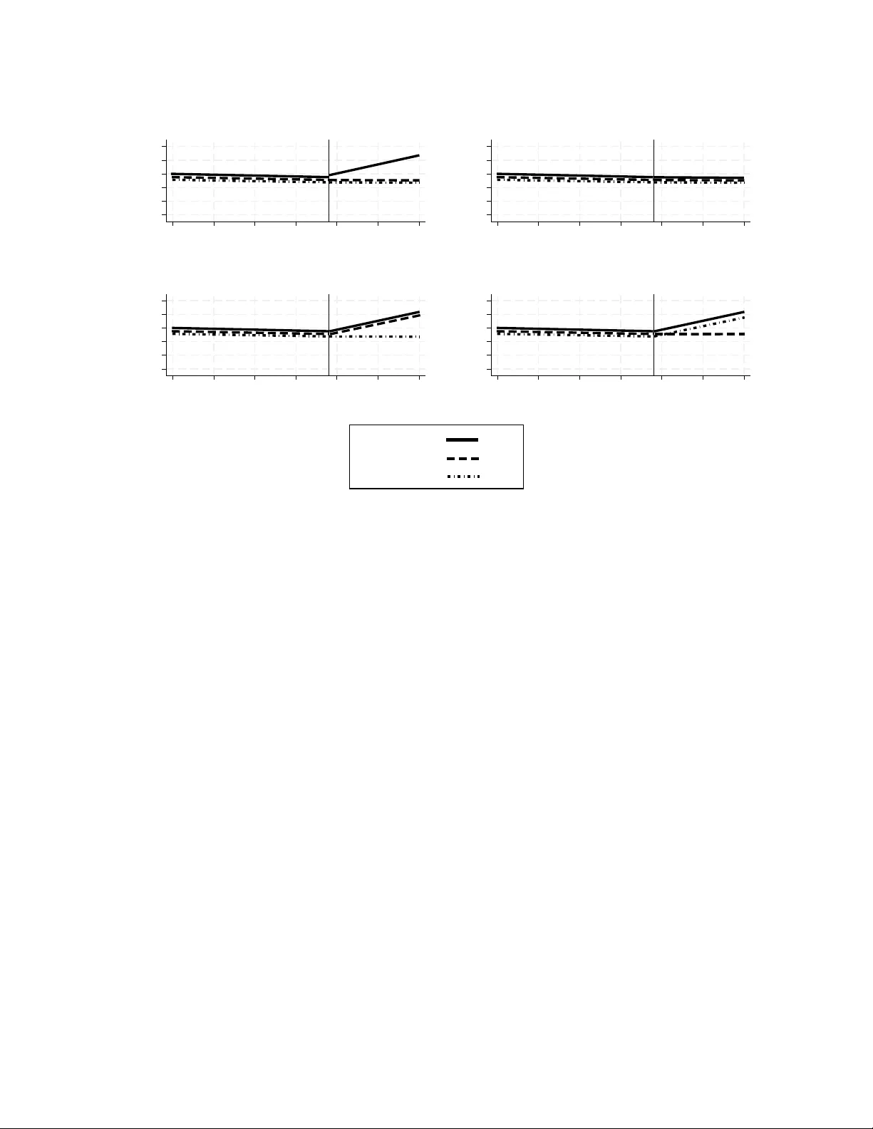
Impro ving causal inference in in terrupted time series analysis: the triple difference design Ariel Linden, DrPH Univ ersity of California, San F rancisco Departmen t of Medicine Division of Clinical Informatics & Digital T ransformation ariel.linden@ucsf.edu Abstract Bac kground: In terrupted time series analysis (ITSA) is a v aluable quasi- exp erimen tal design for ev aluating health p olicy and in terven tion effects. While m ultiple-group ITSA (MG-ITSA) strengthens causal inference b y incorp orating a con- trol group, residual confounding from unmeasured time-v arying factors ma y p ersist. The triple-difference in terrupted time series (DDD-ITSA) design extends this frame- w ork by adding a second control group to further isolate treatment effects, y et the design remains underutilized and lacks formal metho dological guidance. Metho ds: This pap er formalizes the DDD-ITSA design for health research. W e sp ecify the underlying regression mo del, define the k ey co efficien ts for estimating level and trend effects, and clarify the interpretation of the triple-difference estimand. W e also illustrate application of the design using a w ork ed example ev aluating the effect of California’s Prop osition 99 cigarette tax increase on p er-capita cigarette sales. Results: The DDD-ITSA mo del pro vides clear parameterization for assessing base- line balance across groups and estimating differential treatmen t effects. In the st ylized Prop osition 99 example, all groups demonstrated balance on pre-interv ention level and trend. The triple-difference estimand revealed a statistically significan t annual net re- duction of -1.76 p er-capita cigarette pac ks in California relativ e to the secondary con trol (P = 0.020; 95% CI: -3.24, -0.28), consistent with the treatmen t effect observed against the primary con trol. The difference-in-differences betw een the tw o control groups was non-significan t, supp orting the v alidity of the comparison. Conclusions: The DDD-ITSA design offers a robust approac h for strengthening causal inferences when tw o-group comparisons may b e confounded. By leveraging an 1 additional con trol group, researc hers can difference out remaining biases and assess ef- fect heterogeneity across subgroups. The up dated itsa pac k age for Stata facilitates implemen tation, making this design accessible for routine application in health p olicy researc h. Careful atten tion to control group selection, baseline balance, and auto corre- lation remains essential for v alid in terpretation. Keyw ords difference-in-difference-in-differences, triple differences, in terrupted time series analysis, con- trolled in terrupted time series analysis, m ultiple-group in terrupted time series analysis 1 Bac kground In terrupted time series analysis (ITSA) is widely used in healthcare research to estimate the causal effects of in terven tions, policy c hanges, and natural ev en ts when randomized designs are infeasible. The approac h relies on sequential outcome measuremen ts collected at equally spaced in terv als, typically aggregated at th e unit lev el (e.g., hospitals, regions, or p opulations) and summarized as rates, counts, or mean exp enditures. In its canonical form, a single unit is exposed to an interv ention that is hypothesized to generate a structural c hange (“in terruption”) in the lev el and/or slop e of the outcome pro cess at a kno wn p oin t in time [ 1 , 2 ]. Iden tification in this framework is achiev ed b y using the pre-interv ention segmen t of the series to extrapolate the coun terfactual p ost-interv ention tra jectory under the assumption that, absen t the in terven tion, the underlying data-generating pro cess would hav e con tin ued unchanged. The use of m ultiple pre-interv ention observ ations partially addresses threats such as regression to the mean and improv es internal v alidit y relativ e to simpler b efore–after comparisons [ 1 – 3 ]. Despite these strengths, single-group ITSA (SG-ITSA) rests on the strong iden tifying assumption that no unmeasured, time-v arying confounders or coinciden t even ts affect the outcome at the time of in terv en tion. When this assumption is violated (suc h as in the presence of secular trends, an ticipatory b eha vior, or concurren t p olicy changes), SG-ITSA ma y pro duce biased estimates of the in terv en tion effect. Empirical evidence indicates that SG-ITSA can yield misleading inferences when pre-in terv en tion trends already exhibit direc- tional change or when external influences evolv e con temp oraneously with the interv ention [ 4 – 6 ]. Multiple-group or controlled ITSA (MG-ITSA) addresses these threats by introducing con trol units that w ere not exposed to the interv ention but share similar baseline lev els, pre- 2 in terv en tion trends, and observ ed c haracteristics with the treated unit [ 7 – 9 ]. By differencing outcomes b et w een treated and con trol series ov er time, MG-ITSA relaxes the strong assump- tion of stable counterfactual trends within a single unit and instead relies on a parallel-trends- t yp e assumption across groups [ 7 , 9 ]. Under this framework, causal effects are iden tified b y remo ving secular trends and common sho c ks that affect all units similarly , aligning MG- ITSA conceptually with difference-in-differences estimators [ 10 ]. How ev er, when treatmen t effects are exp ected to v ary across an additional dimension, suc h as subp opulations , exp o- sure in tensit y , or p olicy eligibilit y , standard MG-ITSA may remain insufficient to isolate the causal effect of in terest. A triple-difference in terrupted time series (DDD-ITSA) design extends the logic of the MG-ITSA by adding a second con trol group for comparison. This approach mirrors the difference-in-differences-in-differences (DDD) framew ork in the econometrics literature, where an additional difference is used to remo ve remaining confounding that may persist after a standard tw o-group comparison [ 11 ]. In the ITSA con text, the triple-difference estimator captures whether the p ost-in terv ention c hange in level and/or trend for the treated group is larger (or smaller) for the subgroup of in terest than would b e exp ected based on concurrent c hanges in con trol groups and comparison subgroups. By differencing across time, groups, and subgroups sim ultaneously , the DDD-ITSA design strengthens causal iden tification un- der assumptions analogous to those in the difference-in-differences (DiD) literature, namely that, absen t the in terv en tion, these differences w ould ha v e ev olv ed similarly o v er time [ 10 ]. Applications that explicitly implement a DDD-ITSA framew ork remain relatively un- common in the literature. One applied example is the ev aluation of Maryland’s global budget rev enue (GBR) mo del, where researc hers used an interrupted time-series design with difference-in-differences comparisons and a triple differences analysis to assess changes in emergency department utilization, admissions, and revisits follo wing GBR implementation, including how these trends v aried across racial/ethnic and pa y er groups [ 12 ]. In this study , the triple-difference comp onent help ed iden tify differen tial effects of the policy on emer- gency department return outcomes across subp opulations b ey ond general statewide trends and group-lev el effects. Another example is researc h on the effects of the Affordable Care A ct (ACA) on health insurance co verage among Latino subgroups, whic h combined ITSA with triple-difference mo dels to ev aluate heterogeneous c hanges in uninsured rates asso ciated with the A CA and Medicaid expansion across multiple Latino ethnic groups [ 13 ]. This pap er formalizes the DDD-ITSA framew ork for applied health researc h. W e describe the design, detail the underlying statistical model, clarify the interpretation of the key co- efficien ts that iden tify lev el and trend effects, and presen t a w ork ed empirical example to illustrate implemen tation and in terpretation. W e also provide practical guidance regarding 3 iden tification assumptions, model sp ecification, and appropriate use cases for the design. T o facilitate applied use, the itsa pack age for Stata [ 7 ] has been up dated to estimate DDD- ITSA mo dels, enabling researchers to easily implement the approach using their data. 2 Metho ds 2.1 The DDD-ITSA design The DDD-ITSA design is an extension of the MG-ITSA design to an additional control group that is either geographically distant from the treatment and primary control groups, or comprises a differen t demographic that still allo ws for comparison (e.g., t yp e of insurance co v erage, differen t medical condition, ethnicit y , etc.). This second con trol group ma y b e though t of as adding a “doubly robustness” prop ert y to the analysis, in that it provides a second opportunity to get the causal inference correct if the treatment versus primary con trol is confounded. Figure 1 illustrates four of the man y p oten tial outcome scenarios that we could anticipate in the DDD-ITSA design when emphasizing differences in trends: (A) a treatmen t effect in the primary analysis and secondary analysis; (B) no treatment effect in either the primary or secondary analysis; (C) a treatmen t effect in the secondary analysis but not in the primary analysis (evidence of confounding); and (D) a treatment effect in the primary analysis but not in the secondary analysis (suggesting external influences or spillo v er affecting the secondary con trol). 4 10 20 30 40 50 60 Outcome 1 2 3 4 5 6 7 Time (A) 10 20 30 40 50 60 Outcome 1 2 3 4 5 6 7 Time (B) 10 20 30 40 50 60 Outcome 1 2 3 4 5 6 7 Time (C) 10 20 30 40 50 60 Outcome 1 2 3 4 5 6 7 Time (D) Treated: Control 1: Control 2: Figure 1: F our general outcome scenarios for the DDD-ITSA (A) treatment effect in both primary and secondary analyses, (B) no treatmen t effect, (C) treatment effect in secondary analysis only , (D) treatment effect in primary only . 2.2 The DDD-ITSA mo del The DDD-ITSA regression mo del is an extension of the MG-ITSA [ 5 , 7 , 14 ] and assumes the follo wing form: Y t = β 0 + β 1 T t + β 2 X t + β 3 X t T t + β 4 Z 1 + β 5 Z 1 T t + β 6 Z 1 X t + β 7 Z 1 X t T t + β 8 Z 2 + β 9 Z 2 T t + β 10 Z 2 X t + β 11 Z 2 X t T t + ϵ t (1) where Y t is the aggregated outcome v ariable measured at eac h time-p oint t , T t is the time since the start of the study , X t is a dumm y v ariable representing the treatmen t (pre- treatmen t p erio ds = 0, otherwise 1), Z 1 is a dummy v ariable to denote the treatment unit and Z 2 is a dummy v ariable to denote the second con trol group. Therefore, all v ariables and co efficients that include Z 1 are equiv alent to those in an MG-ITSA mo del in whic h the treatment unit is compared to the control group, and all v ariables and co efficien ts that include Z 2 compare the second con trol group to the first control group. More sp ecifically , β 4 represen ts the difference in the lev el (intercept) of the dep endent 5 v ariable b etw een treatmen t and the first control group prior to the interv ention, β 5 represen ts the difference in the slop e (trend) of the dep enden t v ariable b et w een treatmen t and the first con trol group prior to the in terv en tion, β 6 indicates the difference b et w een treatmen t and the first control group in the level of the dep enden t v ariable immediately following in tro duction of the interv ention, and β 7 represen ts the difference b etw een treatmen t and the first control group in the slop e (trend) of the dependent v ariable after initiation of the in terv en tion compared with pre-in terv en tion. Similarly , β 8 represen ts the difference in the level (in tercept) of the dep endent v ariable b et w een the second control group and the first control group prior to the interv ention, β 9 represen ts the difference in the slop e (trend) of the dep endent v ariable b et w een the second con trol and the first con trol group prior to the interv ention, β 10 indicates the difference b e- t w een the second control group and the first con trol group in the lev el of the dep enden t v ariable immediately following in tro duction of the interv ention, and β 11 represen ts the dif- ference b et w een the second control group and the first con trol group in the slop e (trend) of the dep enden t v ariable after initiation of the interv en tion compared with pre-in terv en tion. When the random error terms follow an AR(1) pro cess, ϵ t = ρϵ t − 1 + u t (2) where the auto correlation parameter ρ is the correlation co efficien t betw een adjacen t error terms suc h that | ρ | < 1 , and the disturbances u t are indep enden t N (0 , σ 2 ) [ 15 ]. T able 1 presents the co efficients and linear combination terms for the pre-treatment and p ost-treatmen t trends of each of the three groups, and T able 2 presen ts the d ifference-in- differences of trend comparisons b etw een groups. T able 1: Pre-treatment and p ost-treatment trends, by group Group Pre-treatmen t (X = 0) P ost-treatmen t (X = 1) Pre–p ost trend c hange Con trol 1 (Z1 = 0, Z2 = 0) β 1 β 1 + β 3 β 3 T reatmen t (Z1 = 1, Z2 = 0) β 1 + β 5 β 1 + β 3 + β 5 + β 7 β 3 + β 7 Con trol 2 (Z2 = 1, Z1 = 0) β 1 + β 9 β 1 + β 3 + β 9 + β 11 β 3 + β 11 6 T able 2: Difference-in-differences (trend change) comparisons b etw een groups Comparison DiD Simplified expression T reatmen t vs Con trol 1 ( β 3 + β 7 ) − β 3 β 7 Con trol 2 vs Con trol 1 ( β 3 + β 11 ) − β 3 β 11 T reatmen t vs Con trol 2 ( β 3 + β 7 ) − ( β 3 + β 11 ) β 7 − β 11 T ables 3 and 4 presen t the analogous co efficients and linear com bination terms for the pre- treatmen t and p ost-treatment level changes of eac h of the three groups and their resp ective difference in differences. T able 3: Pre-treatment and p ost-treatment levels, by group Group Pre-treatmen t (X = 0) P ost-treatmen t (X = 1) Pre–p ost lev el c hange Con trol 1 (Z1 = 0, Z2 = 0) β 0 β 0 + β 2 β 2 T reatmen t (Z1 = 1, Z2 = 0) β 0 + β 4 β 0 + β 2 + β 4 + β 6 β 2 + β 6 Con trol 2 (Z2 = 1, Z1 = 0) β 0 + β 8 β 0 + β 2 + β 8 + β 10 β 2 + β 10 T able 4: Difference-in-differences (level change) comparisons b etw een groups Comparison DiD Simplified expression T reatmen t vs Con trol 1 ( β 2 + β 6 ) − β 2 β 6 Con trol 2 vs Con trol 1 ( β 2 + β 10 ) − β 2 β 10 T reatmen t vs Con trol 2 ( β 2 + β 6 ) − ( β 2 + β 10 ) β 6 − β 10 2.3 Assessing balance on baseline lev el and trend In non-exp erimen tal settings, it is critical to ev aluate whether the treatmen t and control groups are balanced in b oth the level and slop e of the outcome v ariable prior to the in ter- v en tion. Balance across groups in baseline levels and trends can b e formally assessed using the co efficien ts from Equation (1). Sp ecifically , statistically insignificant estimates of β 4 and β 5 indicate no systematic differences b etw een the treatment group and the primary control group in pre-interv ention levels and trends, resp ectively . Lik ewise, statistical insignificance of the linear combinations ( β 4 − β 8 ) and ( β 5 − β 9 ) suggests baseline equiv alence b etw een the treatmen t group and the secondary control group in levels and trends. Finally , statistically 7 insignifican t β 8 and β 9 imply balance b et w een the tw o con trol groups in pre-treatment levels and tra jectories. Although multiple baseline trend comparisons are ev aluated, Olden and Mø en [ 11 ] demon- strate that iden tification of the DDD estimator do es not require t w o indep endent parallel trends assumptions. The intuition is that the DDD estimator can b e interpreted as the difference b et w een tw o p otentially biased difference-in-differences estimators. As long as the bias comp onen t is iden tical across these estimators, it differences out, yielding an unbiased DDD estimate. Consequently , only a single parallel trends condition is required for causal in terpretation. 2.4 Example The following example illustrates the analysis of the DDD-ITSA design using data from California’s 1988 enactmen t of Prop osition 99, a voter-appro v ed initiative that increased the cigarette excise tax by $0.25 p er pac k and funded statewide an ti-smoking efforts. The outcome examined is p er-capita cigarette sales (packs), measured ann ually at the state lev el from 1970 to 2000, with 1989 marking the first p ost-interv ention y ear. The dataset includes cigarette sales and four co v ariates: av erage retail cigarette price, logged p er-capita p ersonal income, p er-capita b eer consumption, and the share of the p opulation aged 15–24. F or exp osition purposes, Idaho and Mon tana are assigned to the primary control group and Colorado as the secondary control state. These states w ere iden tified as balanced matc hes to California (the treated state) on baseline level and trend of cigarette sales using the itsamatch program in Stata [ 8 ]. W e analyze the model using the DDD-ITSA feature in the itsa program for Stata [ 7 ]. Regression with Newey–W est standard errors is sp ecified, with a single lag autoregressive structure (AR1). The Stata p ost-estimation command lincom is used to compute W ald estimates for linear com binations of coefficients. The exact co de used in this example is provided in the App endix. 3 Results T able 5 presen ts the regression results for the DDD-ITSA mo del. First, we review how well the groups are balanced on baseline level and trend. β 4 and β 5 indicate that California and the primary control states are balanced on baseline lev el and trend. Linear com binations indicate that California and Colorado are also balanced. Finally , β 8 and β 9 indicate that the t w o con trol groups are balanced. Next, w e ev aluate treatment effects. β 7 indicates that California exp erienced a statistically 8 significan t ann ual net reduction of -2.07 p er-capita cigarette sales compared to the primary con trol states. Similarly , the linear combination ( β 7 − β 11 ) indicates a statistically significant ann ual net decrease relative to the secondary control. The β 11 co efficien t indicates that the difference-in-differences b et w een the t w o con trol groups w as non-statistically significan t. T able 5: Regression results for the DDD-ITSA mo del Co efficien t Estimate Std Err Z P 95% LCL 95% UCL β 0 126.40 4.58 27.57 0.00 117.41 135.38 β 1 − 1.43 0.43 − 3.35 0.00 − 2.27 − 0.59 β 2 − 11.43 4.46 − 2.56 0.01 − 20.17 − 2.68 β 3 0.58 0.61 0.95 0.35 − 0.62 1.78 β 4 5.83 6.20 0.94 0.35 − 6.33 17.98 β 5 − 0.35 0.57 − 0.61 0.54 − 1.47 0.77 β 6 − 8.63 6.44 − 1.34 0.18 − 21.25 3.98 β 7 − 2.07 0.75 − 2.77 0.01 − 3.54 − 0.61 β 8 12.29 6.84 1.80 0.07 − 1.11 25.70 β 9 − 0.10 0.69 − 0.15 0.88 − 1.46 1.25 β 10 − 6.48 7.75 − 0.84 0.40 − 21.67 8.70 β 11 − 0.31 0.88 − 0.35 0.72 − 2.03 1.41 Note: Standard errors are Newey–W est AR(1) adjusted. 9 40 60 80 100 120 140 Cigarette sales per-capita (in packs) 1970 1980 1990 2000 Year California: Actual Predicted Control 1: Actual Predicted Control 2: Actual Predicted GLM model: family(Gaussian), link(Identity) with Newey-West standard errors - lag(1) Intervention starts: 1989 Three-Group Comparison: California, Control 1, and Control 2 Figure 2: Graphic displa y of the DDD-ITSA outcomes pro duced by the itsa pac k age in Stata. 4 Discussion This pap er formalizes the triple-difference in terrupted time series (DDD-ITSA) design, an extension of the multiple-group ITSA framew ork that incorp orates an additional con trol group to strengthen causal iden tification in health p olicy and interv ention researc h. The DDD-ITSA approac h combines the structural time-series logic of ITSA with the econometric rigor of difference-in-differences-in-differences estimators, offering researchers a p o w erful to ol for estimating causal effects when standard tw o-group comparisons may remain confounded b y unmeasured time-v arying factors. The key contributions of this pap er are the explicit articulation of the DDD-ITSA mo del, including clear parameter in terpretation, and the w ork ed example to illustrate the practical application of the DDD-ITSA design. Researc hers implemen ting DDD-ITSA face several issues with the design that require care- ful consideration. First, the choice of primary and secondary con trol groups is substantiv ely imp ortan t and should b e guided b y conten t exp ertise and empirical balance assessments. The primary control should be as similar as p ossible to the treatmen t unit on observed c har- acteristics and pre-treatment trends [ 7 , 9 ], while the secondary control provides an additional la y er of adjustment, ideally one that shares the primary control’s susceptibility to common 10 sho c ks but differs in wa ys that help isolate treatment effects. Second, when the p o ol of p oten tial controls is sufficien tly large, increasing the n um b er of units assigned to each con trol group should b e considered. Linden [ 16 ] found that adding more con trol units in the MG-ITSA design reduced standard errors and increased p ow er. By extension, incorp orating additional comparison groups in a DDD-ITSA would similarly enhance precision by providing more stable estimates of the coun terfactual trends across m ultiple dimensions. Third, researc hers should review auto correlation and partial autocorrelation functions [ 17 ] and formally test for auto correlation using appropriate diagnostics (e.g., the actest com- mand in Stata [ 18 ]) and sp ecify error structures accordingly , whether through New ey–W est standard errors [ 19 ], Prais–Winsten regression [ 20 ], Co c hrane–Orcutt regression [ 21 ], instru- men tal v ariables [ 22 ], or other time-series estimators [ 23 , 24 ]. F ourth, researc hers should endeav or to collect as long of time series data as p ossible. Lin- den [ 16 ] found that in the MG-ITSA context, a longer study p erio d provides the necessary statistical resolution to detect trend-based effects and mitigates the bias introduced by au- to correlation, whic h can otherwise sev erely undermine p ow er. Researc hers should therefore design DDD-ITSA studies with the exp ectation that detecting a meaningful trend change will demand a longer time horizon than simpler designs might require. Finally , Linden [ 16 ] found that introducing treatment at the midp oin t of the time series maximizes p o w er for iden tifying trend c hanges in the MG-ITSA. This w ould apply equally to DDD-ITSA designs, as balanced pre- and p ost-treatmen t p erio ds would minimize standard errors across all in teraction terms. The DDD-ITSA design is particularly w ell-suited to sev eral common scenarios in health services and p olicy researc h. First, when researc hers susp ect that t w o-group comparisons ma y b e confounded b y concurrent p olicy changes, economic sho c ks, or secular trends that differen tially affect subgroups, the addition of a second con trol group can difference out these common sources of bias. Second, DDD-ITSA is v aluable when treatmen t effects are exp ected to v ary across an additional dimension suc h as demographic subgroups, pay er t yp es, or clinical conditions. Third, the design is appropriate when researchers ha v e access to m ultiple p oten tial con trol groups but are uncertain which provides the most v alid counterfactual. 5 Conclusion The DDD-ITSA design offers a v aluable addition to the health p olicy researcher’s to olkit, extending the logic of m ultiple-group in terrupted time series to address remaining sources of confounding through the inclusion of a second control group. By differencing across time, 11 groups, and subgroups, DDD-ITSA enhances the credibilit y of causal claims in observ ational in terrupted time-series settings when suitable contro l series are av ailable. References [1] Donald T. Campb ell and Julian C. Stanley . Exp erimental and Quasi-Exp erimental Designs for R ese ar ch . Rand McNally , Chicago, 1966. [2] William R. Shadish, Thomas D. Cook, and Donald T. Campbell. Exp erimental and Quasi-Exp erimental Designs for Gener alize d Causal Infer enc e . Houghton Mifflin, Boston, 2002. [3] Ariel Linden. Assessing regression to the mean effects in health care initiatives. BMC Me d R es Metho dol , 13:119, 2013. URL https://doi.org/10.1186/ 1471- 2288- 13- 119 . [4] Ariel Linden and P aul R. Y arnold. Using mac hine learning to iden tify structural breaks in single-group in terrupted time series designs. Journal of Evaluation in Clinic al Pr ac- tic e , 22:855–859, 2016. URL https://doi.org/10.1111/jep.12544 . [5] Ariel Linden. Challenges to v alidit y in single-group interrupted time series analysis. Journal of Evaluation in Clinic al Pr actic e , 23:413–418, 2017. URL https://doi. org/10.1111/jep.12638 . [6] Ariel Linden. P ersisten t threats to v alidity in single-group in terrupted time series anal- ysis with a crossov er design. Journal of Evaluation in Clinic al Pr actic e , 23:419–425, 2017. URL https://doi.org/10.1111/jep.12668 . [7] Ariel Linden. Conducting in terrupted time-series analysis for single- and multiple- group comparisons. Stata Journal , 15(2):480–500, 2015. URL https://doi.org/ 10.1177/1536867X1501500208 . [8] Alb erto Abadie, Alexis Diamond, and Jens Hainmueller. Syn thetic control methods for comparativ e case studies: estimating the effect of california’s tobacco con trol program. Journal of the Americ an Statistic al Asso ciation , 105(490):493–505, 2010. URL https: //doi.org/10.1198/jasa.2009.ap08746 . [9] Ariel Linden. A matching framew ork to impro ve causal inference in interrupted time- series analysis. Journal of Evaluation in Clinic al Pr actic e , 24:408–415, 2018. URL https://doi.org/10.1111/jep.12874 . 12 [10] Andrew M. Ry an, Ev angelos Kon topantelis, Ariel Linden, and James F. Burgess. No w trending: Coping with non-parallel trends in difference-in-differences analysis. Stat Metho ds Me d R es , 28:3697–3711, 2019. URL https://doi.org/10.1177/ 0962280218814570 . [11] Andreas Olden and Jarle Møen. The triple difference estimator. The Ec onometrics Journal , 25:531–553, 2022. URL https://doi.org/10.1093/ectj/utac010 . [12] Omar J. Galarraga, Derek DeLia, Jing Huang, Christine W o o dco c k, Richard J. F air- banks, and Jesse M. Pines. Effects of maryland’s global budget rev enue mo del on emer- gency department utilization and revisits. A c ademic Emer gency Me dicine , 29:83–94, 2022. URL https://doi.org/10.1111/acem.14351 . [13] Gilb ert Gonzales and Benjamin D. Sommers. Intra-ethnic cov erage disparities among latinos and the effects of health reform. He alth Servic es R ese ar ch , 53:1373–1386, 2018. URL https://doi.org/10.1111/1475- 6773.12733 . [14] Ariel Linden. A comprehensiv e set of p ostestimation measures to enrich in terrupted time-series analysis. Stata Journal , 17:73–88, 2017. URL https://doi.org/10. 1177/1536867X1701700105 . [15] Mic hael H. Kutner, Christopher J. Nach tsheim, John Neter, and William Li. Applie d Line ar Statistic al Mo dels . McGra w-Hill Irwin, New Y ork, 5th edition, 2005. [16] Ariel Linden. Po w er considerations for multiple-group (controlled) int errupted time series analysis: A comprehensive simulation study . Evaluation & the He alth Pr ofessions , 2026. URL https://doi.org/10.1177/01632787261428159 . [17] George E.P . Box, Gwilym M. Jenkins, Gregory C. Reinsel, and Greta M. Ljung. Time Series A nalysis: F or e c asting and Contr ol . Wiley , Hob oken, 5th edition, 2016. [18] Christopher F. Baum and Margaret E. Shaffer. Actest. stata mo dule to p erform cum by- h uizinga general test for auto correlation in time series, 2013. Statistical Softw are Comp onen ts s457668, Boston College Department of Economics. Downloadable from: h ttp://ideas.rep ec.org/c/b o c/b o co de/s457668.html. [19] Whitney K. Newey and Kenneth D. W est. A simple, positive semi-definite, heterosk edas- ticit y and auto correlation consisten t cov ariance matrix. Ec onometric a , 55:703–708, 1987. 13 [20] S. J. Prais and C. B. Winsten. T rend estimators and serial correlation. T echnical rep ort, Co wles Commission, 1954. [21] Donald Cochrane and Guy H. Orcutt. Application of least squares regression to rela- tionships containing auto-correlated error terms. Journal of the Americ an Statistic al Asso ciation , 44:32–61, 1949. URL https://doi.org/10.2307/2280349 . [22] Ariel Linden and John L. A dams. Ev aluating disease management programme effectiv e- ness: an in tro duction to instrumental v ariables. Journal of Evaluation in Clinic al Pr ac- tic e , 12:148–154, 2006. URL https://doi.org/10.1111/j.1365- 2753.2006. 00615.x . [23] Andrew C. Harv ey . F or e c asting, structur al time series mo dels and the Kalman filter . Cam bridge Univ ersit y Press, Cam bridge, 1989. [24] W alter Enders. Applie d Ec onometric Time Series . John Wiley & Sons, New Y ork, 2nd edition, 2004. 14 Abbreviations ITSA: In terrupted time series analysis. MG-ITSA: Multiple-group in terrupted time series analysis. SG-ITSA: Single-group in terrupted time series analysis. DiD: Difference-in-differences. DDD-ITSA: T riple difference interrupted time series analysis. CI: Confidence in terv al. GBR: Maryland’s global budget rev en ue (GBR) mo del. A CA: Affordable Care A ct. Supplemen tary Information The App endix con tains Stata co de for replicating the Example. Authors’ con tributions AL conceived the study and its design, conducted all analyses, wrote the man uscript and tak es public resp onsibilit y for its conten t. F unding There w as no funding asso ciated with this work. Declarations Ethics appro v al and consen t to participate: Not applicable. Consen t for publication: Not applicable. Comp eting in terests The author declares no comp eting interests. 15 App endix // Download the most recent version of itsa ssc install itsa, replace // Example use "cigsales.dta", replace // Declare data as time series tsset state year * estimate ITSA model in which California is specified as the * treatment unit (#3 in the data), the treatment period is set * to 1989, the lag is set to 1 (based on actest), the primary * control IDs are 8 and 19 (for Idaho and Montana) and the secondary * control is Colorado (4). We specify that the output should * include post-treatment trends for all groups, and request that * a figure be produced itsa cigsale, treatid(3) trperiod(1989) lag(1) replace /// contid(8 19) contid2(4) posttrend figure * baseline level treatment vs control 1 (beta4) lincom _b[_z1] * baseline trend treatment vs control 1 (beta5) lincom _b[_z1_t] * baseline level control 2 vs control 1 (beta8) lincom _b[_z2] * baseline trend control 2 vs control 1 (beta9) lincom _b[_z2_t] * baseline level treatment vs control 2 (beta4 - beta8) lincom _b[_z1] - _b[_z2] 16 * baseline trend treatment vs control 2 (beta5 - beta9) lincom _b[_z1_t] - _b[_z2_t] * DD trends treatment vs control 1 (beta7) lincom _b[_z1_x_t1989] * DD trends treatment vs control 2 (beta7 - beta11) lincom _b[_z1_x_t1989] - _b[_z2_x_t1989] * DD trends control 1 vs control 2 (beta11) lincom _b[_z2_x_t1989] * DDD-ITSA (beta7 - beta11) lincom _b[_z1_x_t1989] - _b[_z2_x_t1989] 17