Federated Causal Representation Learning in State-Space Systems for Decentralized Counterfactual Reasoning

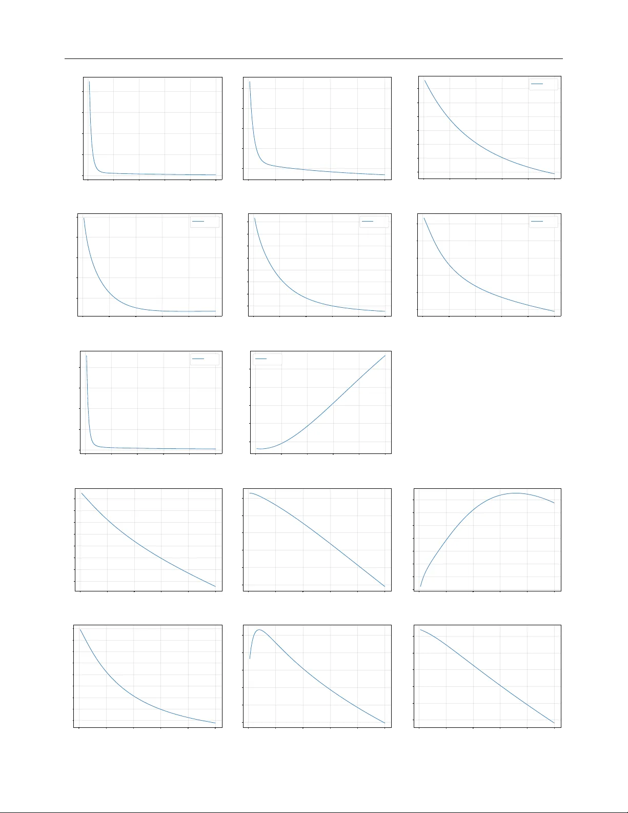
F ederated Causal Represen tation Learning in State-Space Systems for Decen tralized Coun terfactual Reasoning Nazal Mohamed ∗ A yush Mohan ty ∗ , † Nagi Gebraeel Georgia Institute of T echnology , A tlanta, GA 30332, United States of America Georgia Institute of T echnology , A tlanta, GA 30332, United States of America Georgia Institute of T echnology , A tlanta, GA 30332, United States of America Abstract Net works of interdependent industrial assets (clien ts) are tigh tly coupled through physical pro cesses and con trol inputs, raising a k ey question: how would the output of one client change if another client wer e op er ate d diﬀer- ently? This is diﬃcult to answer because clien t-sp eciﬁc data are high-dimensional and priv ate, making centralization of ra w data infeasible. Eac h client also main tains pro- prietary local models that cannot b e mo d- iﬁed. W e prop ose a federated framew ork for causal representation learning in state- space systems that captures interdependen- cies among clients under these constrain ts. Eac h client maps high-dimensional observ a- tions in to lo w-dimensional laten t states that disen tangle in trinsic dynamics from con trol- driv en inﬂuences. A cen tral serv er estimates the global state-transition and control struc- ture. This enables decentralized coun terfac- tual reasoning where clients predict ho w out- puts w ould c hange under alternative con trol inputs at others while only exc hanging com- pact laten t states. W e pro ve conv ergence to a cen tralized oracle and pro vide priv acy guar- an tees. Our exp eriments demonstrate scal- abilit y , and accurate cross-client coun terfac- tual inference on syn thetic and real-world in- dustrial con trol system datasets. ∗ Equal contribution. † Corresp on ding author: ayushmohanty@gatech.edu 1 In tro duction Complex industrial systems such as oil reﬁneries, w a- ter treatmen t netw orks, and distributed process plants consist of geographically disp ersed y et tigh tly coupled assets (clients) that in teract dynamically through con- trol actions and material ﬂows. A change at one clien t suc h as a pump adjustmen t or v alv e op eration, can causally propagate to others, inﬂuencing b oth perfor- mance and safet y across the netw ork. These interde- p endencies mak e the system vulnerable to cascading disruptions, where lo cal disturbances can escalate in to large-scale op erational failures [Pournaras et al., 2020, Ghosh et al., 2025]. Managing these risks requires causal models that not only identify which clients in- ﬂuence one another, but also reason ab out ho w inter- v entions propagate across the system. Granger causality (GC) is a classical to ol for detecting in terdep endencies in time-series data [Granger, 1969, Gew eke, 1982, T ang et al., 2023]. Y et GC is funda- men tally predictive rather than in terv entional, and th us cannot answer coun terfactual questions such as: how would my output have change d if another client had alter e d its c ontr ol input? Moreov er, GC conﬂates in trinsic state dynamics with control-driv en inﬂuences, lea ving the source of interdependencies ambiguous. In practice, how ev er, op erators often need exactly this t yp e of coun terfactual reasoning [T ang et al., 2023, Ruiz-T agle et al., 2022]. F or instance, assessing “ how r e ducing ﬂow at an upstr e am unit would aﬀe ct down- str e am stability ”, or “ how adjusting a p e er’s c ontr ol set- tings might inﬂuenc e lo c al pr o duct quality ”. Without suc h capabilities, decision-making remains limited to retrosp ectiv e diagnostics rather than proactive inter- v ention planning. Practical constrain ts further com- plicate this problem. Mo dern assets generate high- dimensional sensor data that is exp ensive to transmit, while bandwidth and comm unication limits prev ent cen tralization. Priv acy regulations and conﬁden tial- it y concerns restrict data sharing across organizational b oundaries. Finally , eac h clien t t ypically main tains a proprietary local mo del trained on its own data, whic h m ust remain intact and cannot b e altered in a data analysis pip eline. T o address these c hallenges, w e de- v elop a federated learning framework tailored to dis- F ederated Causal Represen tation Learning for Coun terfactual Reasoning tributed industrial systems. W e fo cus on linear state-space systems, which provide a tractable represen tation of causally interdependent dynamics using lo w-dimensional laten t states. In our framew ork, each client retains its proprietary mo del and maps raw high-dimensional measuremen ts into disen tangled low-dimensional latent states. Sp eciﬁ- cally , at the client lev el, w e utilize a mo deling ap- proac h that separates autoregressive time-series dy- namics from control eﬀects. A central server acting as a conduit b etw een these in terdep endent clients es- timates the global structures for the state-transition and input matrices without direct access to ra w high- dimensional data (measurements). This architecture equips each clien t to answer counterfactual queries, suc h as predicting how its outputs w ould change if another clien t altered its controls without sharing ra w data, inputs, or proprietary models. T o the b est of our kno wledge, this is the ﬁrst w ork to enable decentral- ized coun terfactual reasoning. Main Con tributions. The key tec hnical con tribu- tions of this pap er are as follo ws: • W e employ the “ Ab duction-A ction-Pr e diction ” framew ork of [Pearl, 2009] to formally deriv e the av er- age treatment eﬀect in the federated setting, enabling decen tralized counterfactual reasoning. • W e prop ose a federated learning approach in whic h the serv er explicitly estimates the state-transition and input matrices, while clients learn their implicit eﬀects, without mo ving any priv ate, high-dimensional data. • W e design an iterativ e optimization scheme across serv ers and clien ts that prov ably disentangles autore- gressiv e dynamics from exogenous inputs, a key re- quiremen t for decentralized counterfactual reasoning. • W e pro ve con vergence of the decentralized framew ork to a cen tralized oracle with direct access to all high- dimensional clien t measurements. In addition, we pro- vide diﬀerential priv acy guarantees for the federated proto cols by quantifying the p erturbations required in comm unicated quantities to protect client data. • Exp eriments on syn thetic data v alidate the main claims of the paper w.r.t. counterfactual reasoning, con vergence to a centralized oracle, and diﬀerential priv acy , and further demonstrate robustness and scal- abilit y . Real-world experiments conﬁrm the applica- bilit y of the approach of industrial control systems. 2 Related W ork Causal Inference in Dynamical Systems. Granger causalit y (GC) is the classical tool for detecting predictive dep endencies in time series [Granger, 1969, Gewek e, 1982, Barnett et al., 2009]. Extensions such as structural GC [Eichler, 2010] and causal state-space mo dels [Huang et al., 2019, Mastak ouri et al., 2021] ha v e attempted to incorp o- rate in terven tional seman tics, but they typically as- sume centralized access and conﬂate endogenous dynamics with exogenous inputs. Probabilistic approac hes including dynamic Ba yesian net works [Murph y , 2002] and laten t-v ariable state-space mo dels [Krishnan et al., 2015, F raccaro et al., 2017] impro v e represen tation p ow er but remain predictive in nature. F ederated Causal Discov ery . F ederated learning [McMahan et al., 2017] has b een extended to causal disco very across distributed clients. [Li et al., 2024b] prop ose federated conditional indep endence test- ing for heterogeneous data. [Mian et al., 2022, Mian et al., 2023] introduce regret-based metho ds with priv acy guarantees. F edECE [Y e et al., 2024] es- timates causal eﬀects across institutions using graphi- cal modeling without data sharing. [Zhao et al., 2025] dev elop a distributed annealing algorithm for feder- ated DA G learning under generalized linear models, oﬀering iden tiﬁability guaran tees. More recent w orks address scalability . F edCausal [Y ang et al., 2024] uni- ﬁes lo cal and global optimization through adaptive strategies, while F edCSL [Guo et al., 2024] improv es accuracy with lo cal-to-global learning and weigh ted aggregation. Despite these adv ances, existing meth- o ds focus on structural recov ery or associations. They lac k counterfactual semantics. Causal Represen tation Learning. P earl’s Ab duction–A ction–Prediction (AAP) framew ork [P earl, 2009] formalizes counterfactual inference and underpins mo dern causal reasoning. Extensions such as inv ariant causal prediction [Peters et al., 2016], in- v ariant risk minimization [Arjo vsky et al., 2019], and causal representation learning [Schölk opf et al., 2021, Brehmer et al., 2022, Lipp e et al., 2022] aim to learn in v ariant and interv ention-a ware rep- resen tations. Disen tangled state-space mo d- els [Miladino vić et al., 2019, W eng et al., 2025], and disen tangled representation learning [Li et al., 2024a, W ang et al., 2024] impro ve in- terpretabilit y but assume cen tralized data access. Recen t counterfactual time-series approac hes like [Mastak ouri et al., 2021, T o do et al., 2023] also remain cen tralized. 3 Preliminaries Linear Time Inv ariant (L TI) Systems. The dy- namics of a linear system can b e describ ed by the fol- lo wing L TI state-space equations: h t = A h t − 1 + B u t − 1 + w t − 1 ; y t = C h t + v t , (1) Nazal Mohamed ∗ , A yush Mohan ty ∗ , † , Nagi Gebraeel where h t ∈ R P is the laten t state, u t ∈ R S is the in- put (or con trol), and y t ∈ R D is the measuremen t (also called observ ation or output). The matrices A ∈ R P × P , B ∈ R P × S , and C ∈ R D × P are time- in v ariant state-transition, input, and output matrices, resp ectiv ely . w t − 1 ∼ N (0 , Q w ) , and v t ∼ N (0 , R v ) are the pro cess noise and measuremen t noise, respectively . Structural Causal Mo dels (SCMs). In a causal system, we represent in terdep endencies among v ari- ables using a c ausal gr aph , where no des correspond to v ariables and directed edges enco de direct causal inﬂuence. F or any v ariable X , we denote by P a( X ) the set of its parent no des. W e then distinguish b e- t ween tw o types of v ariables: (1) Exo genous variables ( U ) are determined outside the system b eing mo deled. They capture background factors, noise, or unobserved inﬂuences not explained by the mo del itself. (2) En- do genous variables ( H ) are determined within the sys- tem by structural equations. Structural assignments E generate each endogenous v ariable H from its paren ts P a( H ) in the causal graph and an asso ciated exoge- nous v ariable U such that, H := E (P a( H ) , U ) . A structural causal mo del (SCM) sp eciﬁes an ordered triplet ⟨ U, H, E ⟩ , providing a principled w ay to infer causal relationships in a system. In terven tion. An interv ention, denoted by do( u = u ′ ) , u ∈ U , is an experiment performed by re- placing the structural assignment of u with the constan t u ′ and leaving all other assignments un- c hanged. [Pearl, 2009]’s Ab duction-Action-Prediction (AAP) sc heme giv en b elo w, pro vides a principled ap- proac h to infer the consequence of interv ention: (1) Ab duction: infer laten t quantities from past ob- serv ations; (2) Action: encode the interv ention by mo difying the relev an t structural assignment(s); (3) Prediction: propagate the interv ened mo del forward to obtain in terven tional outcomes. Predicting the consequence of interv ention is the k ey to answ ering coun terfactual questions suc h as, “ what would h ∈ H have b e en under a diﬀer ent value of u ? ”. A common w ay to quan tify suc h eﬀects is via the av- er age tr e atment eﬀe ct (A TE), deﬁned as follows: AT E : = E [ h | do( u = u 1 )] − E [ h | do( u = u 0 )] , (2) In other words, AT E measures the exp ected c hange in the endogenous v ariable h when the exogeneous v ari- able u is set to u 1 instead of u 0 through in terven tion. L TI system as an SCM. The L TI state-space system in (1) can b e alternatively view ed as an SCM, where h t and y t are endogenous v ariables, and u t − 1 , w t and v t are exogenous. The input u t − 1 is not go verned b y the system dynamics but externally sp eciﬁed. Hence u t − 1 qualiﬁes as an interv ention v ariable. The state h t cannot b e observed directly (thus, called latent state ) and has to b e estimated from the measurements y t , using a Kalman ﬁlter [Kalman, 1960] . 4 Coun terfactuals for L TI Systems Prop osition 4.1 shows that only the matrices C and B parameterize the AT E of externally applied inputs on do wnstream measurements. Prop osition 4.1. L et the input to an L TI system b e u t − 1 = u 0 . Then the A TE on me asur ements y t under the intervention do( u t − 1 = u 1 ) e quals C B ( u 1 − u 0 ) . 4.1 Multi-Clien t System W e consider a multi-client L TI state-space setting with M clients (subsystems). Client m ∈ { 1 , . . . , M } has lo cal state h t m ∈ R P m , input u t m ∈ R U m , and measure- men t y t m ∈ R D m , with D m >> P m , U m . The joint dynamics follo w Eq (1). W e further assume: Assumption 4.2. The matrix C is blo ck-diagonal. R ationale. b ehind Assumption 4.2 In man y engi- neered s ystems, sensors are tied to a physical subsys- tem, so y t m dep ends only on h t m , i.e., y t m = C mm h t m . Under Assumption 4.2, Prop osition 4.1 giv es the fol- lo wing causal eﬀect ( AT E ) in the multi-clien t setting: E [ y t m | do( u t − 1 n = u n 1 )] − E [ y t m | do( u n = u n 0 )] = C mm B mn ( u n 1 − u n 0 ) ∀ m  = n (3) Equation 3 addresses the coun terfactual query: Q1. “What would y t m have b e en if client n ’s input u t − 1 n had change d?” Problem F ormulation. W e study coun terfactual reasoning in m ulti-client L TI systems under decen- tralized constraints. Eac h client observ es only high- dimensional local measurements y t m , with no access to other clients’ data. The goal is to estimate cross-client causal eﬀects B mn (Eq. 3) that answer Q1 , while re- sp ecting priv acy and communication limits. Role of A in Latent-State Reco very . Although the AT E in Prop osition 4.1 dep ends only on B mn , esti- mating it in practice requires access to latent states h t . These states evolv e according to the transition matrix A : without mo deling A , one cannot disentangle (i) endogenous propagation of past states via A mn from (ii) exogenous input eﬀects via B mn . Thus, learning A mn ∀ m, n is essential b oth for reco vering h t and for isolating the causal con tribution of B mn . F ederated Causal Represen tation Learning for Coun terfactual Reasoning 4.2 Decen tralized Setting While Eq. 3 identiﬁes B mn as the k ey parameter for coun terfactual reasoning, estimating it in a decentral- ized en vironment is challenging due to: (1) Partial observ abilit y: Only noisy measurements y t are ob- serv ed lo cally . Recov ering B mn requires ﬁrst inferring laten t states h t b y modeling A and then separating the eﬀects of A mn and B mn . (2) Data sharing con- strain ts: Clients cannot share ra w y t due to priv acy , and y t is often high-dimensional, making direct com- m unication infeasible. These constrain ts motiv ate a federated approach to estimate { A mn , B mn } . Eac h client transmits low- dimensional state estimates ˆ h t m , and inputs u t m to a co- ordinating server, without exp osing ra w measurements y t m . The server explicitly estimates { A mn , B mn } us- ing aggregated { ˆ h t , u t } across clien ts (extending prior w ork, e.g., [Mohan ty et al., 2025], whic h solved only the special case B ≡ 0 ). This enables server-side coun- terfactual reasoning via Eq. 3. Key c hallenge for clien ts. Unlike the server, client m observ es only its o wn ˆ h t m and u t m , and receiv es no states or inputs from others. Lo cal estimates, there- fore, conﬂate tw o sources of v ariation: (i) endogenous propagation of past states (through A mn ) and (ii) exogenous input eﬀects (through B mn ). T o supp ort Q1 lo cally , clients m ust learn represen tations in which these eﬀects are disen tangled , so that B mn can b e isolated and used in Eq. 3. Our training metho dology is designed to enforce this disentanglemen t at the client lev el, while relying only on server communications. 5 F ederated T raining Metho dology 5.1 Proprietary Clien t Mo del Assumption 5.1. Eac h clien t m knows its local blo ck matrices A mm , B mm , and C mm . R ationale b ehind Assumption 5.1 The matrices A mm , B mm , and C mm corresp ond to the diagonal blo c ks of the global state-transition matrix A , input matrix B , and output matrix C of the L TI system. These lo cal blocks do not aﬀect coun terfactual query Q1 . Moreo ver, if not pre-sp eciﬁed, they can be readily estimated b y each client using only its own data. Notation. Kalman ﬁltering distinguishes a one-step- ahead pr e dicte d state from a r eﬁne d estimate d state . W e denote b y h t the one-step-ahead prediction at time t (based on information up to t − 1 ), and by ˆ h t the reﬁned estimate after observing y t at time t . The proprietary clien t mo del is a Kalman ﬁlter (in general it can b e an y state estimator), whic h makes use of the lo cal blo ck matrices A mm , B mm , C mm , the lo cal measurement y t m , and input u t m to compute a pr e dicte d state h t m,c and a r eﬁne d estimate ˆ h t m,c . Assumption 5.2. The proprietary mo del provides b oth h t m,c (predicted state) and ˆ h t m,c (reﬁned esti- mate), which are treated as given inputs to our fed- erated learning metho d. Limitation of the Proprietary Mo del. Since the proprietary model relies exclusiv ely on lo cal informa- tion (i.e., A mm , B mm , C mm , y t m , and u t m ), it cannot capture cross-clien t interdependencies and is therefore unable to answ er query Q1 (Section 4.2). 5.2 Augmen ted Client Model T o ov ercome the limitations of the proprietary mo del, w e augment it with additional ML parameters, yield- ing an augmente d client mo del . The gov erning equa- tions are: h t m,a = A mm ˆ h t − 1 m,a + B mm u t − 1 m + ϕ m , (4) ˆ h t m,a = ˆ h t m,c + θ m y t m . (5) Here, h t m,a denotes the augmente d pr e dicte d state , and ˆ h t m,a the augmente d r eﬁne d estimate , whic h extends the proprietary estimate ˆ h t m,c b y incorporating the learned parameter θ m . The corresp onding client loss is deﬁned as, L t m,a : = ∥ r t m,a ∥ 2 2 , where w e hav e, r t m,a = y t m − ˜ y t m,a , with ˜ y t m,a = C mm h t m,a . (6) Therefore, the clien t loss is just a r e c onstruction loss with ˜ y t m,a denoting the r e c onstructe d me asur ement , whic h serves as the k ey output for counterfactual anal- ysis (used later in Section 6). P arameter up dating. Each clien t updates ϕ m and θ m b y com bining gradien ts from its o wn loss L m,a with gradien ts derived from the server loss L s . Imp or- tan tly , the server nev er sends raw data; instead, it comm unicates only the gradien ts with resp ect to the augmen ted states, namely ∇ h t m,a L s and ∇ ˆ h t − 1 m,a L s . The clien t then uses the chain rule of partial deriv atives (pro of can b e found in the App endix) to compute: ∇ θ m L s = T X t =1  A ⊤ mm · ∇ h t m,a L s + ∇ ˆ h t − 1 m,a L s  y t − 1 m ⊤ (7) ∇ ϕ m L s = T X t =1 ∇ h t m,a L s . (8) Using the locally computed ∇ θ m L s , ∇ ϕ m L s , and learn- ing rates η 1 , η 2 , γ 1 , γ 2 , the up dated parameters are Nazal Mohamed ∗ , A yush Mohan ty ∗ , † , Nagi Gebraeel Figure 1: A simpliﬁed view of the computation inside the client m then giv en by , θ k +1 m = θ k m − η 1 ∇ θ m L m,a − η 2 ∇ θ m L s , (9) ϕ k +1 m = ϕ k m − γ 1 ∇ ϕ m L m,a − γ 2 ∇ ϕ m L s . (10) Claim 5.3. The lo cal client parameters θ m and ϕ m learn to enco de cross-client interdependencies arising from oﬀ-diagonal blo c ks A mn and B mn ( n  = m ). Intuition on Claim 5.3 . Although each clien t ob- serv es only local data, the server gradien ts ∇ θ m L s and ∇ ϕ m L s implicitly carry information ab out how other clien ts’ data inﬂuence the server loss. When combined with lo cal gradients, these up dates guide θ m and ϕ m to represen t cross-client eﬀects, enabling the augmen ted mo del to capture interdependencies that the propri- etary mo del cannot. A theoretical pro of is pro vided in Section 6, with empirical v alidation in Section 9. Comm. to the Server: Each client m sends { ˆ h t m,c , ˆ h t m,a , h t m,a , u t m } to the serv er. 5.3 Serv er Mo del Assumption 5.4. The diagonal blocks A mm and B mm are kno wn at the server. R ationale b ehind Assumption 5.4. F rom Assump- tion 5.1, each client m already has access to A mm and B mm . Their eﬀects are purely lo cal and do not inﬂu- ence cross-clien t coun terfactual reasoning, hence they are not cen tral to our analysis. Communicating them to the serv er, therefore, incurs only a ﬁxed one-time cost during initialization. After receiving ˆ h t m,c , ˆ h t m,a , h t m,a , and u t m from client m , together with the kno wn diagonal blo cks { A mm , B mm } and the curren t estimates of { ˆ A mn , ˆ B mn } n  = m , the serv er predicts the future state h t m,s , and computes a residual r t m,s giv en by , h t m,s = A mm ˆ h t − 1 m,c + X n  = m ˆ A mn ˆ h t − 1 n,c + B mm u t − 1 m + X n  = m ˆ B mn u t − 1 n , and (11) r t m,s = h t m,a − h t m,s . (12) T o learn an estimate of the oﬀ-diagonal blo cks { A mn , B mn } n  = m , the serv er minimizes a loss, L s := 1 T T X t =1 M X m =1  ∥ r t m,s ∥ 2 2 + ξ m   A mm  ˆ h t − 1 m,a − ˆ h t − 1 m,c  − X n  = m ˆ A mn ˆ h t − 1 n,c   2 2  | {z } D (13) Claim 5.5. With large ξ m , D disentangles cross-client eﬀects of A mn (endogenous) and B mn (exogeneous). Claim 5.5 ensures that each clien t separates the con- tributions of A mn and B mn when learning its param- eters θ m and ϕ m , respectively . Theoretical proof of Claim 5.5 is pro vided in Section 6. P arameter Up dating. The server updates the oﬀ- diagonal blo c ks by blo ck gradient descent, ˆ A k +1 mn = ˆ A k mn − α A ∇ ˆ A k mn L s , and (14) ˆ B k +1 mn = ˆ B k mn − α B ∇ ˆ B k mn L s , ∀ n  = m. (15) Comm. to the Clients. The server comm unicates gradien ts ∇ h t m,a L s to eac h client m . 5.4 Ov erhead Comm unication. A t eac h training round, ev- ery clien t transmits laten t states and inputs F ederated Causal Represen tation Learning for Coun terfactual Reasoning { ˆ h t m,c , ˆ h t m,a , h t m,a , u t m } of dimension O ( P m + U m ) to the server, and receives gradien t up dates of size O ( P m ) , leading to a p er-round communication cost of O ( M ( P + U )) , where P = P m P m and U = P m U m . Computation. The server p erforms blo ck gradien t descen t o ver matrices { A mn , B mn } , with per-round complexit y O ( M 2 P 2 + M 2 U 2 ) in the worst case. Eac h clien t’s lo cal updates (Eqs. 10) require O ( T P 2 m ) opera- tions p er round, dominated b y matrix-vector pro ducts with dimension P m . 6 Inference: Causal Representations The training in Section 5 is iterative: (i) the serv er learns cross-clien t dep endencies via oﬀ-diagonal blo cks A mn , B mn ( n  = m ), and (ii) clien ts enco de them in lo- cal parameters θ m , ϕ m . Cross-clien t information ﬂows to the serv er through lo w-dimensional states, and to clien ts via serv er-loss gradien ts L s (Claim 5.3). W e no w show these gradients explicitly enco de A mn , B mn : The gradients sen t from the serv er to the client m are ∇ h t m,a L s deﬁned as, ∇ h t m,a L s := 2 T  h t m,a −  A mm ˆ h t − 1 m,c + X n  = m ˆ A mn ˆ h t − 1 n,c + B mm u t − 1 m + X n  = m ˆ B mn u t − 1 n   . (16) Eq. 16 shows that ∇ h t m,a L s dep ends on b oth A mn and B mn . By Eqs. 8–10, θ m and ϕ m th us learn an entan- gled representation of these eﬀects. Y et coun terfac- tuals in Eq. 3 require isolating B mn from A mn , making en tanglement a barrier to answ ering query Q1 . The next section addresses disentanglemen t via Claim 5.5. F or all clients m , at any time t , the following hold: Theorem 6.1. In Eq. 13, as ξ → ∞ , the stationary p oints ˆ A ∗ mn of the server and θ ∗ m of the clients satisfy E h A mm θ ∗ m y t m i = E h X n  = m ˆ A ∗ mn ˆ h t n,c i ∀ m  = n. (17) Corollary 6.2. As ξ → ∞ , the stationary p oints B ∗ mn of the server and ϕ ∗ m of the clients satisfy ϕ ∗ m = E h X n  = m ˆ B ∗ mn u t n i ∀ m  = n. (18) With suﬃcien tly large ξ m (Eq. 13), Theorem 6.1 and Corollary 6.2 ensure client parameters disen tangle A mn and B mn , ev en though the server communicated gradien ts ∇ h t m,a L s remain en tangled (Eq (16)). W e hav e established that the clien t m implicitly learns P n  = m B mn u t n (in expectation) through its augmented parameter ϕ m , while the server explicitly learns B mn for all n  = m . Consequen tly , b oth can answer coun- terfactual queries, alb eit with diﬀeren t ﬁdelity: (1) Server. The server ev aluates counterfactuals at the state lev el, estimating the following quantit y: E [ h t m,s | do( u t − 1 n = u n 1 )] − E [ h t m,s | do( u t − 1 n = u n 0 )] = B mn ( u n 1 − u n 0 ) , (19) answ ering: Q2. “What would h t m,s have b e en if client n ’s input u t − 1 n had change d?” (2) Client. The client ev aluates counterfactuals at the measuremen t level, essentially estimating: E [ ˜ y t m,a | do( ϕ m = ϕ m 1 )] − E [ ˜ y t m,a | do( ϕ m = ϕ m 0 )] = C mm ( ϕ m 1 − ϕ m 0 ) , = C mm · E h X n  = m B mn ( u n 1 − u n 0 ) i (20) whic h, by Corollary 6.2, answers the query: Q3. “What would ˜ y t m,a have b e en if the aggr e gate d eﬀe cts of inputs fr om other clients had change d?” Th us, the server isolates the eﬀect of a sp eciﬁc clien t’s input u n , while the client reasons only through the aggregated inﬂuence P n  = m B mn u n enco ded in ϕ m . 7 Con v ergence to a Cen tralized Mo del W e consider a cen tralized mo del as the or acle for our approac h. Since each proprietary client mo del is a lo- cal Kalman ﬁlter (KF), a natural oracle that encodes full cross-clien t causalit y is a centralized KF with ac- cess to all clients’ data and full knowledge of ( A, B ) . Th us the oracle’s dynamics are gov erned as: h t o = A ˆ h t − 1 o + B u t − 1 ; ˜ y t o = C h t o , (21) r t o = y t − ˜ y t o ; and ˆ h t o = h t o + K t o r t o , (22) where K t o is the cen tralized Kalman gain. Assumption 7.1 ( Exogenous Input ) . The input u t is zero-mean, stationary , er go dic , and indep endent of noises w t , and v t (Eq (1)), with E ∥ u t ∥ 2 < ∞ . More- o ver, u t is p ersistently excite d of order L if there exist L ∈ N and α > 0 such that 1 L t + L − 1 X k = t u k u k ⊤ ⪰ αI d u for all t. (23) Lemma 7.2 ( Normal equations ) . Under Assump- tion 7.1, at stationary p oints we have, E  ( C mm A mm ) ⊤ r ∗ ,t m,a ( y t − 1 m ) ⊤  = 0 , E  C ⊤ mm r ∗ ,t m,a  = 0 . (24) wher e, r ∗ ,t m,a = y t m − ˜ y t m,a ( θ ∗ m , ϕ ∗ m ) same as Eq (6) Nazal Mohamed ∗ , A yush Mohan ty ∗ , † , Nagi Gebraeel Theorem 7.3 ( Conv ergence to the oracle ) . As- sume C mm A mm is ful l c olumn r ank and Assump- tion 7.1 holds. Then in the r e gime ξ m → ∞ we have, E  ˜ y t m,o − ˜ y t m,a ( θ ∗ m , ϕ ∗ m )  = J m E[ z t − 1 m ] . (25) wher e, z t − 1 m := [ y t − 1 m ; u t − 1 ; ˆ h t − 1 m,c ] , Σ z := E[ z t − 1 m z t − 1 ⊤ m ] , e t := C mm  A mm θ ∗ m y t − 1 m − P n  = m ˆ A ∗ mn ˆ h t − 1 n,c + ϕ ∗ m − P n  = m ˆ B ∗ mn u t − 1 n  , and J m := E[ e t z t − 1 ⊤ m ]Σ − 1 z . Lemma 7.2 states that, at stationarity , the augmented clien t residual is orthogonal (in expectation) to the lo cal regressors it uses ( y t m , u t , ˆ h t m,c ); i.e., no further linear correction along those directions can reduce the residual. Theorem 7.3 then says that, when the clien t models hav e causal disentanglemen t ( ξ m → ∞ regime), the federated reconstruction matc hes the or- acle in exp ectation up to a bias term J m E[ z t − 1 m ] . 8 Priv acy Analysis W e conduct a detailed diﬀeren tial priv acy analysis of the prop osed framew ork in the App endix. 9 Exp erimen ts 9.1 Syn thetic Datasets W e establish the p erformance of our algorithm on a m ulti-client L TI system describ ed in Section 4.1. Un- less otherwise sp eciﬁed, w e focus our exp eriments on a t wo-clien t system with P m = 2 , U m = 2 , and D m = 2 for m = { 1 , 2 } . A one-w ay directed dep endency with A 12 = 0 and A 21  = 0 is considered for the ease of in- terpretation. The elements of input v ectors are i.i.d. samples from a normal distribution N (0 , 1) . Clients use (4) and (5) to compute augmented state predic- tions and estimates. The proprietary client state es- timate ˆ h t m,c is estimated in our exp erimen t using a Kalman ﬁlter that uses only the client-speciﬁc (local) diagonal blo cks ( A mm , B mm , C mm ) . The comm unica- tion and training pro ceed as detailed in Section 5. The serv er maintains its state estimate according to (11), computed using current estimates of { ˆ A mn } n  = m and { ˆ B mn } n  = m . Hardw are. 2022 MacBo ok Air (Apple M2, 8-core CPU, 8-core GPU, 16-core Neural Engine), 8 GB uni- ﬁed memory , 256 GB SSD. No discrete GPU. The mo del w as trained on a time series of length 9000. T raining curves plotted are obtained after running 10 Monte-Carlo sim ulations. Each elemen t of initial v alues of ϕ 0 m , θ 0 m , { ˆ A 0 mn } n  = m and { ˆ B 0 mn } n  = m for all m = 1 , 2 , · · · , M are independently sampled from nor- mal distributions. Global loss and client loss for b oth clients during train- ing are plotted in Fig. 2a-2c. The baseline used for comparison is the time-av eraged norm of resid- uals of the proprietary client model ( r t m,c := y t m − C mm h t m,c ). As training progresses, the augmen ted clien t loss L m,a outp erforms the proprietary client loss. Th us, the parameters θ m and ϕ m , through the aug- men ted client, enco de cross-client interdependencies from oﬀ-diagonal blocks of A and B - whic h is not captured by the proprietary client mo del, v alidating Claim 5.3. The ﬁnal estimated v alues of oﬀ-diagonal blocks of A and B are given in T able 1. Comparison with more baselines and further details are discussed in the Ap- p endix. Disen tanglement : The disentanglemen t p enalty D at the serv er is plotted in Fig. 3a, and the diﬀerence δ d :=    ϕ m − 1 T P T t =1  P n  = m ˆ B mn u t − 1 n     2 is plotted for b oth clients in Fig. 3b and 3c. This demonstrates that not only server eﬀectively disentangle the eﬀect of inputs from the states, but it is also propagated to the resp ectiv e clients accordingly . The results plotted here are obtained b y directly opti- mizing the server loss function (13) with the disen tan- glemen t p enalty ξ and tuning the learning rates. It w as observ ed that direct implemen tation of the p enalty- based disentanglemen t could make the framew ork un- stable for large v alues ξ - whic h is a requiremen t for eﬀectiv e disentanglemen t. This issue can b e mitigated b y implementing an Augmented Lagrangian metho d ([Bertsek as and Rheinboldt, 2014]). Augmented La- grangian metho d results in b etter disentanglemen t while keeping the framew ork stable, but might con- v erge sub-optimal solution compared to the p enalty- based disen tanglement. More details regarding this can b e found in the App endix. Scalabillit y : (i) W e ﬁx the num b er of clien ts M , state dimension P m for each client and v ary the measure- men t dimension D m . (ii) The state dimension P m and measuremen t dimension D m for each client is ﬁxed and the n umber of clients are v aried. More details of scal- abilit y exp eriments can b e found in the App endix. 9.2 Real-w orld Datasets 9.2.1 Exp erimen tal Setting W e ev aluate our approach using tw o industrial cyb er- securit y datasets: (1) HAI and (2) SW aT, both of whic h provide realistic testb ed environmen ts. HAI. The HAI dataset records time-series data from an industrial control system testb ed enhanced with a Hardware-in-the-Loop (HIL) sim ulator. This sim- F ederated Causal Represen tation Learning for Coun terfactual Reasoning 0 100 200 300 400 500 Number of iterations ( k ) 0 . 10 0 . 15 0 . 20 0 . 25 0 . 30 0 . 35 0 . 40 Server Loss ( L k s ) (a) Global loss L k s 0 100 200 300 400 500 Number of iterations ( k ) 0 . 2 0 . 4 0 . 6 0 . 8 1 . 0 1 . 2 Client residual L k 1 ,a 1 T P T t =1 k r t 1 ,c k 2 2 (b) Client 1: losses 0 100 200 300 400 500 Number of iterations ( k ) 0 . 1 0 . 2 0 . 3 0 . 4 0 . 5 0 . 6 Client residual L k 2 ,a 1 T P T t =1 k r t 2 ,c k 2 2 (c) Client 2: losses Figure 2: Global loss at the server and losses at the clien t from diﬀeren t mo dels (augmen ted clien t loss: L k m,a , proprietary clien t loss: 1 T P T t =1   r t m,c   2 2 are plotted against the n umber of iterations ( k ). T able 1: Estimated vs Ground T ruth oﬀ-diagonal blo cks of A and B Estimated ˆ A 21 Ground truth A 21 Estimated ˆ A 12 Ground truth A 12  0 . 0044 0 . 0540 − 0 . 1073 − 0 . 2030   − 0 . 2588 0 . 2990 − 0 . 2554 − 0 . 2567   0 . 0789 − 0 . 0533 0 . 0775 − 0 . 2305   0 . 1334 − 1 . 0546 − 0 . 9507 − 0 . 3099  Estimated ˆ B 21 Ground truth B 21 Estimated ˆ B 12 Ground truth B 12  − 0 . 0323 0 . 0220 0 . 0089 0 . 1012   0 0 0 0 . 0392   − 0 . 0617 − 0 . 0451 0 . 0092 0 . 0103   0 . 0544 0 0 . 2182 0 . 1836  ulator em ulates steam-turbine p ow er generation and pump ed-storage h ydrop ow er. The testb ed consists of four pro cesses: (P1) Boiler, (P2) T urbine, (P3) W ater T reatment, and (P4) HIL Simulation. SW aT. The SW aT dataset originates from a six-stage w ater treatment plan t testb ed. Each stage is treated as a clien t in our exp eriments. 9.2.2 Prepro cessing W e apply separate prepro cessing pipelines to the tw o datasets. HAI. All sensor measurements are ﬁrst normalized to ensure consisten t scaling. A subspace identiﬁcation metho d is then applied to ﬁt an L TI system, yielding a state-transition matrix A , input matrix B , and an observ ation matrix C . The dimensionality of the state space P m is determined using the singular v alue de- ca y of the Hankel matrix. Since the initial C is not blo c k diagonal, we p erform L 2 -norm based threshold- ing to assign each state v ariable to a sp eciﬁc pro cess and construct a blo ck diagonal C . With this structure in place, A and B are re-estimated via least squares. SW aT. F or each client, only those v ariables with a P earson correlation greater than 0.3 with other clien ts are retained. After this selection, the same subspace iden tiﬁcation and re-estimation steps as in the HAI case are p erformed. 9.2.3 Results Due to space constrain ts, w e pro vide results for both real-w orld datasets in the App endix. 0 100 200 300 400 500 Number of iterations ( k ) 0 . 0013 0 . 0014 0 . 0015 0 . 0016 0 . 0017 0 . 0018 0 . 0019 0 . 0020 0 . 0021 (a) Disentang. p enalty: D 0 100 200 300 400 500 Number of iterations ( k ) 0 . 05 0 . 10 0 . 15 0 . 20 0 . 25 0 . 30 0 . 35 0 . 40 (b) Client 1: δ d 0 100 200 300 400 500 Number of iterations ( k ) 0 . 05 0 . 10 0 . 15 0 . 20 0 . 25 0 . 30 (c) Client 2: δ d Figure 3: Disen tanglement penalty at the server and δ d at the clients vs Number of iterations 10 Limitations Our framework assumes linear time-inv ariant state- space mo dels, whic h may not capture real-w orld sce- Nazal Mohamed ∗ , A yush Mohan ty ∗ , † , Nagi Gebraeel narios such as nonlinear or time-v arying dynamics. It relies on accurate proprietary lo cal mo dels and kno wn lo cal matrices, which ma y b e unrealistic in practice. While comm unication is more eﬃcient than ra w data sharing, federated training still introduces ov erhead. Moreo ver, clien ts can only infer aggregated input ef- fects (in exp ectation), lac king the granularit y of server- side reasoning. Con v ergence guarantees only hold up to a bias in reconstruction. References [Arjo vsky et al., 2019] Arjovsky , M., Bottou, L., Gul- ra jani, I., and Lop ez-Paz, D. (2019). Inv arian t risk minimization. arXiv pr eprint arXiv:1907.02893 . [Asc her et al., 1995] Ascher, U. M., Ruuth, S. J., and W etton, B. T. R. (1995). Implicit-explicit metho ds for time-dep endent partial diﬀerential equations. SIAM Journal on Numeric al A nalysis , 32(3):797– 823. [Barnett et al., 2009] Barnett, L., Barrett, A. B., and Seth, A. K. (2009). Granger causalit y and transfer en tropy are equiv alent for gaussian v ariables. Phys- ic al R eview L etters , 103(23):238701. [Bertsek as and Rheinboldt, 2014] Bertsek as, D. and Rhein b oldt, W. (2014). Constr aine d Optimization and L agr ange Multiplier Metho ds . Computer science and applied mathematics. A cademic Press. [Brehmer et al., 2022] Brehmer, J., De Haan, P ., Lipp e, P ., and Cohen, T. S. (2022). W eakly super- vised causal represen tation learning. A dvanc es in Neur al Information Pr o c essing Systems , 35:38319– 38331. [Eic hler, 2010] Eichler, M. (2010). Granger causalit y and path diagrams for multiv ariate time series. Sta- tistic al Mo del ling , 10(3):233–255. [F raccaro et al., 2017] F raccaro, M., Kamronn, S., P a- quet, U., and Winther, O. (2017). A disentangled recognition and nonlinear dynamics mo del for unsu- p ervised learning. A dvanc es in neur al information pr o c essing systems , 30. [Gew eke, 1982] Gewek e, J. (1982). Measuremen t of linear dep endence and feedbac k b etw een multiple time series. Journal of the A meric an Statistic al As- so ciation , 77(378):304–313. [Ghosh et al., 2025] Ghosh, S. S., Dwivedi, A., T a jer, A., Y eo, K., and Giﬀord, W. M. (2025). Cascading failure prediction via causal inference. IEEE T r ans- actions on Power Systems , 40(4):3361–3373. [Granger, 1969] Granger, C. W. (1969). Inv estigating causal relations by econometric mo dels and cross- sp ectral metho ds. Ec onometric a , 37(3):424–438. [Guo et al., 2024] Guo, X., Y u, K., Liu, L., and Li, J. (2024). F edcsl: A scalable and accurate approach to federated causal structure learning. Pr o c e e dings of the AAAI Confer enc e on Artiﬁcial Intel ligenc e , 38(11):12235–12243. [Huang et al., 2019] Huang, B., Zhang, K., Gong, M., and Glymour, C. (2019). Causal discov ery and fore- casting in nonstationary en vironments with state- space mo dels. In International c onfer enc e on ma- chine le arning , pages 2901–2910. Pmlr. [Kalman, 1960] Kalman, R. E. (1960). A new ap- proac h to linear ﬁltering and prediction problems. T r ansactions of the ASME–Journal of Basic Engi- ne ering , 82(Series D):35–45. [Krishnan et al., 2015] Krishnan, R. G., Shalit, U., and Son tag, D. (2015). Deep k alman ﬁlters. arXiv pr eprint arXiv:1511.05121 . [Li et al., 2024a] Li, A., Pan, Y., and Barein b oim, E. (2024a). Disentangled representation learning in non-mark ovian causal systems. A dvanc es in Neur al Information Pr o c essing Systems , 37:104843–104903. [Li et al., 2024b] Li, L., Ng, I., Luo, G., Huang, B., Chen, G., Liu, T., Gu, B., and Zhang, K. (2024b). F ederated causal discov ery from hetero- geneous data. arXiv pr eprint arXiv:2402.13241 . [Lipp e et al., 2022] Lipp e, P ., Magliacane, S., Löwe, S., Asano, Y. M., Cohen, T., and Ga vves, S. (2022). Citris: Causal iden tiﬁability from temporal in ter- v ened sequences. In International Confer enc e on Machine L e arning , pages 13557–13603. PMLR. [Mastak ouri et al., 2021] Mastakouri, A., Rohde, D., and Schölk opf, B. (2021). Necessary and suﬃcien t conditions for c ausal feature selection in time series with laten t confounders. In NeurIPS . [Math ur and Tipp enhauer, 2016] Mathur, A. P . and Tipp enhauer, N. O. (2016). Swat: a water treatmen t testb ed for research and training on ics security . In 2016 International W orkshop on Cyb er-physic al Sys- tems for Smart W ater Networks (CySW ater) , pages 31–36. [McMahan et al., 2017] McMahan, B., Mo ore, E., Ra- mage, D., Hampson, S., and y Arcas, B. (2017). Comm unication-eﬃcient learning of deep netw orks from decentralized data. In Artiﬁcial Intel ligenc e and Statistics (AIST A TS) . F ederated Causal Represen tation Learning for Coun terfactual Reasoning [Mian et al., 2022] Mian, O., Kaltenp oth, D., and Kamp, M. (2022). Regret-based federated causal disco very . In Le, T. D., Liu, L., Kıcıman, E., T ri- an tafyllou, S., and Liu, H., editors, Pr o c e e dings of The KDD’22 W orkshop on Causal Disc overy , v ol- ume 185 of Pr o c e e dings of Machine L e arning R e- se ar ch , pages 61–69. PMLR. [Mian et al., 2023] Mian, O., Kaltenp oth, D., Kamp, M., and V reeken, J. (2023). Nothing but regrets—priv acy-preserving federated causal discov- ery . In International Confer enc e on A rtiﬁcial Intel- ligenc e and Statistics , pages 8263–8278. PMLR. [Miladino vić et al., 2019] Miladinović, Ð., Gondal, M. W., Schölk opf, B., Buhmann, J. M., and Bauer, S. (2019). Disen tangled state space represen tations. arXiv pr eprint arXiv:1906.03255 . [Mohan ty et al., 2025] Mohant y , A., Mohamed, N., Ramanan, P ., and Gebraeel, N. (2025). F ederated granger causalit y learning for in terdep endent clients with state space represen tation. In The Thirte enth International Confer enc e on L e arning R epr esenta- tions . [Murph y , 2002] Murphy , K. P . (2002). Dynamic Bayesian networks: r epr esentation, infer enc e and le arning . PhD thesis, UC Berkeley . [P earl, 2009] Pearl, J. (2009). Causality: Mo dels, R e a- soning and Infer enc e . Cambridge Univ ersity Press, 2 edition. [P eters et al., 2016] Peters, J., Bühlmann, P ., and Meinshausen, N. (2016). Causal inference by using in v ariant prediction: identiﬁcation and conﬁdence in terv als. Journal of the R oyal Statistic al So ciety Series B: Statistic al Metho dolo gy , 78(5):947–1012. [P ournaras et al., 2020] Pournaras, E., T aormina, R., Thapa, M., Galelli, S., P alleti, V., and K o oij, R. (2020). Cascading failures in interconnected p ow er- to-w ater netw orks. SIGMETRICS Perform. Eval. R ev. , 47(4):16–20. [Ruiz-T agle et al., 2022] Ruiz-T agle, A., Lop ez- Droguett, E., and Groth, K. M. (2022). A nov el probabilistic approach to counterfactual reasoning in system safet y . R eliability Engine ering & System Safety , 228:108785. [Sc hölkopf et al., 2021] Schölk opf, B., Lo catello, F., Bauer, S., Ke, N. R., Kalch brenner, N., Goy al, A., and Bengio, Y. (2021). T ow ard causal representa- tion learning. Pr o c e e dings of the IEEE , 109(5):612– 634. [Shin et al., 2021] Shin, H.-K., Lee, W., Y un, J.-H., and Min, B.-G. (2021). T wo ics securit y datasets and anomaly detection con test on the hil-based aug- men ted ics testb ed. In Cyb er Se curity Exp erimen- tation and T est W orkshop , CSET ’21, page 36–40, New Y ork, NY, USA. Association for Computing Mac hinery . [T ang et al., 2023] T ang, W., Liu, J., Zhou, Y., and Ding, Z. (2023). Causality-guided counterfactual de- biasing for anomaly detection of cyb er-ph ysical sys- tems. IEEE T r ansactions on Industrial Informatics , 20(3):4582–4593. [T o do et al., 2023] T o do, W., Selmani, M., Laurent, B., and Loub es, J.-M. (2023). Counterfactual ex- planation for multiv ariate times series using a con- trastiv e v ariational auto enco der. In ICASSP 2023- 2023 IEEE International Confer enc e on A c oustics, Sp e e ch and Signal Pr o c essing (ICASSP) , pages 1–5. IEEE. [W ang et al., 2024] W ang, X., Chen, H., T ang, S., W u, Z., and Zhu, W. (2024). Disen tangled repre- sen tation learning. IEEE T r ansactions on Pattern A nalysis and Machine Intel ligenc e , 46(12):9677– 9696. [W eng et al., 2025] W eng, Z., Han, J., Jiang, W., and Liu, H. (2025). Sde: A simpliﬁed and disentan- gled dep endency enco ding framework for state space mo dels in time series forecasting. In Pr o c e e dings of the 31st ACM SIGKDD Confer enc e on Know le dge Disc overy and Data Mining V. 2 , pages 3168–3179. [Y ang et al., 2024] Y ang, D., He, X., W ang, J., Y u, G., Domeniconi, C., and Zhang, J. (2024). F ed- erated causality learning with explainable adaptiv e optimization. Pr o c e e dings of the AAAI Confer enc e on Artiﬁcial Intel ligenc e , 38(15):16308–16315. [Y e et al., 2024] Y e, Q., Amini, A. A., and Zhou, Q. (2024). F ederated learning of generalized linear causal netw orks. IEEE T r ansactions on Pattern A nalysis and Machine Intel ligenc e , 46(10):6623– 6636. [Zhao et al., 2025] Zhao, Y., Y u, K., Xiang, G., Guo, X., and Cao, F. (2025). F edece: F ederated estima- tion of causal eﬀect based on causal graphical mo d- eling. IEEE T r ansactions on Artiﬁcial Intel ligenc e , 6(8):2327–2341. Nazal Mohamed ∗ , A yush Mohan ty ∗ , † , Nagi Gebraeel F ederated Causal Repre sentation Learning in State-Space Systems for Decen tralized Coun terfactual Reasoning Supplemen tary Materials Con ten ts A Priv acy Analysis 12 A.1 Notation and Sensitivity . . . . . . . . . . . . . . . . . . . . . . . . . . . . . . . . . . . . . . . . . 12 A.2 Noise Mechanisms and Calibration . . . . . . . . . . . . . . . . . . . . . . . . . . . . . . . . . . . 12 A.3 Comp osition and Post-Processing . . . . . . . . . . . . . . . . . . . . . . . . . . . . . . . . . . . . 13 B Gradien ts Communicated b y the Server 13 C Experiments 14 C.1 A dditional Results on Synthetic Datasets . . . . . . . . . . . . . . . . . . . . . . . . . . . . . . . 14 C.2 Real-w orld Datasets . . . . . . . . . . . . . . . . . . . . . . . . . . . . . . . . . . . . . . . . . . . 16 D Pseudo co de 18 E Pro ofs 18 E.1 Deriv atives of L s with resp ect to clien t parameters θ m and ϕ m . . . . . . . . . . . . . . . . . . . 18 E.2 Prop osition 4.1 . . . . . . . . . . . . . . . . . . . . . . . . . . . . . . . . . . . . . . . . . . . . . . 20 E.3 Theorem 6.1 . . . . . . . . . . . . . . . . . . . . . . . . . . . . . . . . . . . . . . . . . . . . . . . . 21 E.4 Corollary 6.2 . . . . . . . . . . . . . . . . . . . . . . . . . . . . . . . . . . . . . . . . . . . . . . . 21 E.5 Lemma 7.2 . . . . . . . . . . . . . . . . . . . . . . . . . . . . . . . . . . . . . . . . . . . . . . . . 22 E.6 Theorem 7.3 . . . . . . . . . . . . . . . . . . . . . . . . . . . . . . . . . . . . . . . . . . . . . . . . 22 E.7 Lemma A.6 . . . . . . . . . . . . . . . . . . . . . . . . . . . . . . . . . . . . . . . . . . . . . . . . 24 E.8 Lemma A.8 . . . . . . . . . . . . . . . . . . . . . . . . . . . . . . . . . . . . . . . . . . . . . . . . 24 E.9 Prop osition A.11 . . . . . . . . . . . . . . . . . . . . . . . . . . . . . . . . . . . . . . . . . . . . . 24 E.10 Prop osition A.12 . . . . . . . . . . . . . . . . . . . . . . . . . . . . . . . . . . . . . . . . . . . . . 25 E.11 Corollary A.13 . . . . . . . . . . . . . . . . . . . . . . . . . . . . . . . . . . . . . . . . . . . . . . 25 F ederated Causal Represen tation Learning for Coun terfactual Reasoning A Priv acy Analysis A.1 Notation and Sensitivit y Deﬁnition A.1 ( Lo cal dataset and horizon ) . F or each client m , the priv ate dataset is D m = { y t m } T t =1 , collected o ver a ﬁxed horizon T ∈ N . The union D = {D 1 , . . . , D M } denotes all clien ts’ measurement data. Deﬁnition A.2 ( Neighboring datasets ) . T wo global datasets D and D ′ are neighb ors if they diﬀer at a single measuremen t y t ⋆ m ⋆ for some clien t m ⋆ and time t ⋆ . Assumption A.3 ( Bounded and clipp ed signals ) . Input u t m and output (or measurements) y t m are b ounded (to ensure stabilit y of state-spaces), and are clipp ed to those kno wn b ounds: ∥ y t m ∥ 2 ≤ R y , and ∥ u t m ∥ 2 ≤ R u . The maxim um magnitude across all input/output signals is denoted by R max = max( R y , R u ) . R ationale : Clipping in Assumption A.3 ensures b ounded sensitivity prior to noise addition. Assumption A.4 ( Lo cal estimator contractivit y ) . Each clien t’s augmented estimator is con tractive with constan ts L m > 0 and β m ∈ (0 , 1) : ∥ h t m,a − h t ′ m,a ∥ 2 ≤ L m β t − s m ∥ y s m − y s ′ m ∥ 2 , ∀ s ≤ t. R ationale : Assumption A.4 ensures b ounded propagation of p erturbations in lo cal measurements. Let z t m = [ ˆ h t m,c ; ˆ h t m,a ; h t m,a ; u t m ] ∈ R 3 P m + U m b e the message comm unicated from client m to the server. Deﬁnition A.5 ( Message generation map ) . The deterministic, pre-noise mapping from measurements to the transmitted message is giv en as M t m, msg : ( y 1: t m ) 7→ z t m . This map dep ends on the in ternal dynamics of the proprietary and augmen ted estimators. Lemma A.6 ( ℓ 2 -Sensitivit y of clien t messages ) . Under b ounde d me asur ements and c ontr active estimators, ther e exists κ m > 0 such that for any neighb oring datasets D m and D ′ m diﬀering at one y t ⋆ m , ∥M t m, msg ( D m ) − M t m, msg ( D ′ m ) ∥ 2 ≤ ∆ m, msg = κ m R max . Remark A.7 ( Role of blo ck-diagonal C ) . In our paper, the observ ation matrix C is blo ck-diagonal. When C is blo ck-diagonal (so that y t m = C mm h t m ), eac h client’s κ m dep ends only on its o wn lo cal blo ck. The server communicates the gradient g t m := ∇ h t m,a L s to client m . Given the expression of serv er loss L s in Eq (13), the analytical expression of g m can b e computed as, g t m = 2 T  h t m,a − [ A mm ˆ h t − 1 m,c + X n  = m ˆ A mn ˆ h t − 1 n,c + B mm u t − 1 m + X n  = m ˆ B mn u t − 1 n ]  , Lemma A.8 ( ℓ 2 -Sensitivit y of server gradien ts ) . Given the expr ession of g t m ab ove, the sensitivity with r esp e ct to one change d me asur ement y t ⋆ m ′ (for some client m ′ and time t ⋆ ) is b ounde d by ∥ g t m − g t ′ m ∥ 2 ≤ ∆ m, grad = 2 T (1 + ∥ A mm ∥ ) κ m, mix R max , wher e the c onstant κ m, mix is given explicitly as κ m, mix = L m ′   ∥ C mm ∥ + X n  = m  ∥ A mn ∥ β t − t ⋆ n + ∥ B mn ∥    . wher e, L m ′ arises fr om the lo c al c ontr activity b ound in Assumption A.4. A.2 Noise Mec hanisms and Calibration Deﬁnition A.9 ( Clipping constants ) . Each clien t enforces ℓ 2 -norm clipping thresholds C msg , C grad > 0 , so that ∥ z t m ∥ 2 ≤ C msg and ∥ g t m ∥ 2 ≤ C grad for all m, t . These are chosen such that C msg ≥ ∆ m, msg , C grad ≥ ∆ m, grad . where ∆ m, msg and ∆ m, grad denote the ℓ 2 -sensitivities of the clien t message and server gradients, resp ectively . Nazal Mohamed ∗ , A yush Mohan ty ∗ , † , Nagi Gebraeel Deﬁnition A.10 ( P erturbation ) . Priv acy is achiev ed by adding indep endent Gaussian noise: ˜ z t m = z t m + N (0 , σ 2 msg C 2 msg I ) , ˜ g t m = g t m + N (0 , σ 2 grad C 2 grad I ) . Noise m ultipliers σ msg and σ grad are selected to ac hieve target priv acy parameters ( ε, δ ) . Prop osition A.11 ( P er-release Gaussian DP ) . F or the client m ’s message and server gr adient r ele ase me chanisms, the suﬃcient noise multipliers satisfying ( ε, δ ) -DP ar e σ msg ≥ ∆ m, msg C msg s 2 ln  1 . 25 δ  1 ε msg , σ grad ≥ ∆ m, grad C grad s 2 ln  1 . 25 δ  1 ε grad . The Gaussian perturbation scales σ msg and σ grad quan tify priv acy strength for the message and gradient c han- nels. Larger noise yields stronger priv acy at the exp ense of higher v ariance in estimated parameters. Clipping thresholds C msg and C grad cap the maximum inﬂuence of an y single measuremen t y t m , ensuring the injected noise dominates an y one individual’s contribution. A.3 Comp osition and P ost-Pro cessing Prop osition A.12 ( Sequential and joint comp osition of Gaussian mechanisms ) . L et e ach client m r ele ase privatize d messages ˜ z t m and gr adients ˜ g t m over R c ommunic ation r ounds. If e ach me chanism satisﬁes ( ε msg , δ msg ) -DP for messages and ( ε grad , δ grad ) -DP for gr adients, then the c omp osition acr oss al l r ounds satisﬁes,  ε total , δ total  =  R ( ε msg + ε grad ) , R ( δ msg + δ grad )  . Corollary A.13 ( Post-processing in v ariance ) . Al l downstr e am quantities, including the server’s le arne d matric es { ˆ A mn , ˆ B mn } , client p ar ameters { θ m , ϕ m } , and c ounterfactual outputs, r etain the same ( ε, δ ) privacy guar ante e as the privatize d tr aining tr anscript. B Gradien ts Comm unicated by the Serv er Prop osition B.1. Using the chain rule, the derivatives of the server loss L s with r esp e ct to the augmente d client p ar ameters of client m (i.e., ϕ m and θ m ) ar e ∇ θ m L s = T X t =1  A ⊤ mm ∇ h t m,a L s + ∇ ˆ h t − 1 m,a L s  y t − 1 m ⊤ , and ∇ ϕ m L s = T X t =1 ∇ h t m,a L s . Pr o of. F rom the augmented client mo del, h t m,a = A mm ˆ h t − 1 m,a + b t − 1 m + ϕ m , ˆ h t − 1 m,a = c t − 1 m + θ m y t − 1 m . Consider the pro xy loss, ℓ ( h t m,a , ˆ h t − 1 m,a ) : = 1 T T X t =1  ∥ h t m,a − X t m ∥ 2 2 + ξ ∥ A mm ˆ h t − 1 m,a − Z t − 1 m ∥ 2 2  , This pro xy loss follows the same computational graph as the client mo del with, h t = A mm ˆ h t − 1 + b t − 1 + ϕ, ˆ h t − 1 = c t − 1 + θ y t − 1 . Using Einstein index notation , rep eated Latin indices are summed o ver automatically . Indices p, k , r ∈ { 1 , . . . , P m } denote state comp onents and j, s ∈ { 1 , . . . , D m } denote measuremen t components. The Kroneck er delta is δ ij , and subscripts on a v ector or matrix denote its comp onents. F ederated Causal Represen tation Learning for Coun terfactual Reasoning Deriv ativ e with resp ect to θ m . By the chain rule, ∂ ℓ ∂ θ m,rs = 1 T T X t =1 P m X p =1 ∂ ℓ ∂ h t m,a,p ∂ h t m,a,p ∂ θ m,rs + ∂ ℓ ∂ ˆ h t − 1 m,a,p ∂ ˆ h t − 1 m,a,p ∂ θ m,rs ! . F rom h t m,a,p = A mm,pk ˆ h t − 1 m,a,k + b t − 1 m,p + ϕ m,p , ˆ h t − 1 m,a,k = c t − 1 m,k + θ m,kj y t − 1 m,j , w e hav e ∂ ˆ h t − 1 m,a,k ∂ θ m,rs = δ kr y t − 1 m,s , ∂ h t m,a,p ∂ θ m,rs = A mm,pk ∂ ˆ h t − 1 m,a,k ∂ θ m,rs = A mm,pk δ kr y t − 1 m,s = A mm,pr y t − 1 m,s . Hence, ∂ ℓ ∂ θ m,rs = 1 T T X t =1 h ∂ ℓ ∂ h t m,a,p  A mm,pr +  ∂ ℓ ∂ ˆ h t − 1 m,a,p  δ pr i y t − 1 m,s = 1 T T X t =1 h  A ⊤ mm ∇ h t m,a ℓ  r +  ∇ ˆ h t − 1 m,a ℓ  r i y t − 1 m,s . Collecting the ( r , s ) -entries, the matrix form is ∇ θ m ℓ = 1 T T X t =1  A ⊤ mm ∇ h t m,a ℓ + ∇ ˆ h t − 1 m,a ℓ  ( y t − 1 m ) ⊤ . Deriv ativ e with resp ect to ϕ m . Again by the chain rule, ∂ ℓ ∂ ϕ m,a = 1 T T X t =1 P m X p =1 ∂ ℓ ∂ h t m,a,p ∂ h t m,a,p ∂ ϕ m,a = 1 T T X t =1 P m X p =1 ∂ ℓ ∂ h t m,a,p δ pa = 1 T T X t =1 [ ∇ h t m,a ℓ ] a , or in matrix form, ∇ ϕ m ℓ = 1 T T X t =1 ∇ h t m,a ℓ. Finally , replacing ℓ by L s (the factor 1 /T is an inconsequential constant) yields ∇ θ m L s = T X t =1  A ⊤ mm ∇ h t m,a L s + ∇ ˆ h t − 1 m,a L s  y t − 1 m ⊤ , ∇ ϕ m L s = T X t =1 ∇ h t m,a L s , as claimed. C Exp erimen ts C.1 A dditional Results on Synthetic Datasets Augmen ted Lagrangian with IMEX T o robustify training under large p enalty ξ and im- pro ve lo cal disentanglemen t, w e also exp erimented with an Augmented Lagrangian (AL) formula- tion [Bertsek as and Rheinboldt, 2014] combined with an implicit–explicit (IMEX) time discretization [Asc her et al., 1995]. In AL (as opp osed to the P enalt y Metho d (PM) whic h optimizes L s at the serv er), the hard alignment/consensus condition is enforced via a quadratic p enalty and a dual term λ (s imilar to a Lagrangian m ultiplier), i.e., we up date the server and client v ariables by minimizing the AL server loss, L AL = 1 T T X t =1 M X m =1  ∥ r t m,s ∥ 2 2 + λ t ⊤ m D t m + ρ 2 ∥D t m ∥ 2 2  , Nazal Mohamed ∗ , A yush Mohan ty ∗ , † , Nagi Gebraeel 0 100 200 300 400 500 Number of iterations ( k ) 0 . 0 0 . 2 0 . 4 0 . 6 0 . 8 1 . 0 1 . 2 1 . 4 Server Loss ( L k s ) PM AL (a) Server Loss 0 100 200 300 400 500 Number of iterations ( k ) 0 . 002 0 . 004 0 . 006 0 . 008 0 . 010 0 . 012 D PM AL (b) Disentanglemen t constraint D 0 100 200 300 400 500 Number of iterations ( k ) 0 . 2 0 . 4 0 . 6 0 . 8 1 . 0 Client residual PM AL 1 T P T t =1 k r t 1 ,c k 2 2 (c) Client 1: L k 1 ,a 0 100 200 300 400 500 Number of iterations ( k ) 0 . 1 0 . 2 0 . 3 0 . 4 0 . 5 Client residual PM AL 1 T P T t =1 k r t 2 ,c k 2 2 (d) Client 2: L k 2 ,a 0 100 200 300 400 500 Number of iterations ( k ) 0 . 00 0 . 05 0 . 10 0 . 15 0 . 20 0 . 25 0 . 30 δ d 1 PM AL (e) Client 1: δ d 1 0 100 200 300 400 500 Number of iterations ( k ) 0 . 00 0 . 05 0 . 10 0 . 15 0 . 20 0 . 25 δ d 2 PM AL (f ) Clien t 1: δ d 1 Figure 4: Comparison b etw een Penalt y Method (PM) and Augmen ted Lagrangian (AL) for the tw o clien t system. L s , D , Local loss (client residual) L m,a and δ d m vs Number of iterations ( k ) are plotted. Note that we deﬁned δ d m :=    ϕ m − 1 T P T t =1  P n  = m ˆ B mn u t − 1 n     2 where D t m := A mm  ˆ h t − 1 m,a − ˆ h t − 1 m,c  − X n  = m ˆ A mn ˆ h t − 1 n,c and ρ > 0 is the p enalty . Practically , this stabilizes training under large penalties and promotes cleaner separation of clien t-sp eciﬁc and cross-client eﬀects (“disen tanglement”). The trade-oﬀ is that the IMEX/AL step solv es a pro ximal, constraint-regularized surrogate rather than the original unconstrained gradien t step at eac h iteration; hence the ﬁxed p oint can b e sligh tly biased and, in that sense, sub optimal relativ e to our primary (non-AL) metho d, ev en though it is often b etter b ehav ed numerically . F or all our exp eriments, other than for this part, we ha ve implemented the P enalty Method. In Figure 4, w e hav e compared the Penalt y Metho d (PM) and Augmented Lagrangian (AL). The learning curve of AL exhibits larger oscillations but achiev es b etter disentanglemen t quickly at b oth serv er and clients (Figures 4b, 4e and 4f). This suggests in practice we can use a h ybrid sc hedule: use AL as a w arm start to quic kly enforce disentanglemen t, then switc h to PM to achiev e a smo other descent of L s and a marginally b etter ﬁnal ob jectiv e. Scalabilit y: W e study the scalability of our framework in t wo w ays: (i) F or a tw o comp onen t system, we ﬁx the state dimension P m = 2 , input dimension U m = 2 and generate stable L TI systems with measurement dimensions D m = { 16 , 32 , 64 , 128 } . W e rep ort the ﬁnal server loss function L s and the disentanglemen t norm D in T able 2. (ii) The state, input and output dimensions are ﬁxed at P m = 2 , U m = 2 and D m = 8 resp ectively . The num b er of clients are v aried as M = { 2 , 4 , 8 , 16 } . As before, the ﬁnal server loss L s and D are reported in T able 3 T able 2: L s and D b y scaling measurement dim. D m D m = 16 D m = 32 D m = 64 D m = 128 L s D L s D L s D L s D 0.7649 0.0034 1.0987 0.0041 1.4243 0.0046 1.1805 0.0047 F ederated Causal Represen tation Learning for Coun terfactual Reasoning T able 3: Server loss L s b y scaling num b er of clients M M = 2 M = 4 M = 8 M = 16 L s D L s D L s D L s D 0.0744 0.0013 0.0412 0.0010 0.1714 0.0036 0.3825 0.0069 F rom T ables 2 and 3, it is clear that as the observ ation dimension D m and the num b er of clients M increase, the p erformance degrades. Scaling D m impacts the ob jectiv e more: with P m ﬁxed, the mo del must explain an ev er larger output space with a low-dimensional laten t state. This makes the observ ation map C increasingly tall, ampliﬁes estimation v ariance and sensor noise aggregation, and exposes unmo deled sensor-sp eciﬁc dynamics; consequen tly L s rises even though D remains small. Increasing M introduces more inter-clien t couplings (oﬀ- diagonal A mn , B mn blo c ks) and consensus constrain ts to disen tangle; the larger, more heterogeneous optimization also raises gradient v ariance and complicates stepsize selection, leading to a milder but noticeable growth in L s and D . Overall, the disentanglemen t metric remains lo w across all settings ( D ≤ 7 × 10 − 3 ), indicating that the metho d preserv es separation even as scale grows. C.2 Real-w orld Datasets HAI dataset (v21.03) [Shin et al., 2021]: The HAI industrial con trol dataset logs a multi–unit pro cess with four coupled subsystems (clients), whic h we refer to as P1–P4 . T ags are preﬁxed by the pro cess identiﬁer (e.g., P1_ , P2_ , P3_ , P4_ ). Within each pro cess, sensor channels (e.g., level/ﬂo w/pressure/temp erature transmitters) are con tinuous, while actuator/c ommand channels (e.g., v alve commands and pump toggles) are predominantly discrete. In our federated setting w e map client k to pr o c ess P k simply by this preﬁx rule. Inputs U are tak en from actuator/command tags for that pro cess (e.g., FCV/LCV/PCV/PP/ OnOff / AutoGO / RTR families), and outputs Y are the con tinuous transmitter tags (e.g., LIT/FIT/PIT/TIT/SIT/V*T* families), as sp eciﬁed in the HAI tag man ual. Prepro cessing Starting from the vendor CSV logs, w e (i) time-align and parse headers; (ii) remov e c onstant c hannels ov er the full run and re-c heck after truncation; (iii) prune discrete-like signals b efore mo deling (drop b o olean-lik e and quasi-discrete c hannels with lo w transition coun ts or extreme dominance); (iv) split v ariables in to U and Y by tag family and process preﬁx; (v) standardize eac h column by z -scoring and sav e the means/stds; and (vi) ﬁt a cen tralized L T I mo del with unconstrained A, B while enforcing blo ck-diagonal C, Q, R by pro cess. The iden tiﬁed states are then partitioned to pro cesses b y maximizing energy of the corresp onding C -columns on eac h pro cess’ outputs, with a ﬁx-up step to guarantee at least one state p er active pro cess. Figure 5 shows a c onsisten t con vergence story across all panels. The serv er loss L k s (a) decays rapidly in the ﬁrst few dozen iterations and then tapers oﬀ smo othly , indicating a stable approach to a low-loss regime without oscillations. The disen tanglement constraint D (b) follo ws the same pattern, decreasing monotonically and conﬁrming that the consensus/coupling conditions are b eing enforced as optimization pro ceeds. Overall, the results show fast, stable conv ergence on HAI with uniformly small constrain ts and residuals at the end, despite mild p er-clien t diﬀerences in the transient SW aT Dataset [Math ur and Tipp enhauer, 2016] . The Secure W ater T reatment (SW aT) plan t is a six-stage p otable water facility with tightly con trolled pumping, ﬁltration, and disinfection units. T ags follow the instrumen tation man ual con ven tion: pro cess equipment identiﬁers (e.g., MV101, P201, UV401) embed the stage in the leading digit. W e map federated clien ts to stages S1–S6 using this digit. Manipulated v ariables (inputs) come from actuator and command tags—motorised v alves (MV***), pumps (P***), UV toggles, and setp oin t/command c hannels. Measurements (outputs) are the contin uous transmitters: ﬂo w (FIT***), level (LIT***), diﬀeren tial pressure (DPIT***), pressure (PIT***), analogue analysers, etc. Unlike HAI, actuators are almost fully discrete, so we treat them as binary bits (after collapsing o ccasional tri-state enco dings) and reserv e all real-v alued telemetry for outputs. Prepro cessing : (i) promote the ﬁrst row to the header, relab el columns, and align timestamps; (ii) drop constan t c hannels globally and again after truncating to the ﬁrst 30000 samples; (iii) detect and remo ve quasi- discrete or b o olean-like signals on the measuremen t side; (iv) classify each tag in to inputs or outputs using Nazal Mohamed ∗ , A yush Mohan ty ∗ , † , Nagi Gebraeel 0 100 200 300 400 500 Number of iterations ( k ) 50 100 150 200 250 300 350 Server Loss ( L k s ) (a) Server Loss 0 100 200 300 400 500 Number of iterations ( k ) 0 . 02 0 . 03 0 . 04 0 . 05 0 . 06 0 . 07 0 . 08 0 . 09 (b) D 0 100 200 300 400 500 Number of iterations ( k ) 10 20 30 40 50 Client residual L k 1 ,a (c) Client 1: L k 1 ,a 0 100 200 300 400 500 Number of iterations ( k ) 0 25 50 75 100 125 150 175 Client residual L k 2 ,a (d) Client 2: L k 2 ,a 0 100 200 300 400 500 Number of iterations ( k ) 2 . 7 2 . 8 2 . 9 3 . 0 3 . 1 3 . 2 3 . 3 3 . 4 Client residual L k 3 ,a (e) Client 3: L k 3 ,a 0 100 200 300 400 500 Number of iterations ( k ) 3 . 75 3 . 80 3 . 85 3 . 90 3 . 95 4 . 00 Client residual L k 4 ,a (f ) Clien t 4: L k 4 ,a 0 100 200 300 400 500 Number of iterations ( k ) 0 . 45 0 . 50 0 . 55 0 . 60 0 . 65 0 . 70 (g) Client 1: δ d 1 0 100 200 300 400 500 Number of iterations ( k ) 0 . 0 0 . 5 1 . 0 1 . 5 2 . 0 (h) Client 2: δ d 2 0 100 200 300 400 500 Number of iterations ( k ) 0 . 00 0 . 05 0 . 10 0 . 15 0 . 20 0 . 25 0 . 30 0 . 35 (i) Client 3: δ d 3 0 100 200 300 400 500 Number of iterations ( k ) 0 . 000 0 . 025 0 . 050 0 . 075 0 . 100 0 . 125 0 . 150 0 . 175 (j) Client 4: δ d 4 Figure 5: HAI dataset stage-a ware regex heuristics and split p er stage; (v) z-score every column, saving the means/standard deviations; and (vi) add small Gaussian noise to the (otherwise discrete) input channels so the centralized L TI identiﬁcation has non-degenerate excitation. W e then identify a centralized L TI mo del with unconstrained (A, B) but enforce blo c k-diagonal (C, Q, R) b y stage. States are assigned to stages (clients) via the energy of their (C)-columns on eac h stage’s outputs, with a ﬁx-up to ensure ev ery active stage owns at least one state before exporting p er-stage comp onen t folders. F ederated Causal Represen tation Learning for Coun terfactual Reasoning The results from SW aT dataset are plotted in Figure 6. Similar to the results from the HAI dataset, Figure 6 illustrates the conv ergence b ehavior observ ed on the SW aT dataset. The server loss L k s (a) exhibits a sharp initial decline follow ed by a smo oth saturation phase, indicating a stable approach tow ard a lo w-loss regime with no noticeable oscillations. The disentanglemen t constrain t D (b) follo ws a similar monotonic decreasing trend, demonstrating that the consensus and coupling constrain ts are eﬀectively enforced throughout optimization. Due to the large scale of the SW aT dataset and the constraints of a v ailable computational resources, Mon te Carlo sim ulations were not p erformed; consequently , the rep orted results corresp ond to a single represen tative sample path. D Pseudo co de Refer to Algorithm 1 for the pseudo co de of the prop osed federated learning framework. E Pro ofs E.1 Deriv ativ es of L s with resp ect to clien t parameters θ m and ϕ m Prop osition E.1. Using the chain rule, the derivatives of the server loss L s with r esp e ct to the augmente d client p ar ameters of client m (i.e., ϕ m and θ m ) ar e ∇ θ m L s = T X t =1  A ⊤ mm ∇ h t m,a L s + ∇ ˆ h t − 1 m,a L s  y t − 1 m ⊤ , (26) ∇ ϕ m L s = T X t =1 ∇ h t m,a L s . (27) Pr o of. F rom the mo del, h t m,a = A mm ˆ h t − 1 m,a + b t − 1 m + ϕ m , ˆ h t − 1 m,a = c t − 1 m + θ m y t − 1 m . T o make the chain rule b o okkeeping explicit, consider the proxy loss ℓ ( h t , ˆ h t − 1 ) : = 1 T T X t =1  ∥ h t − X t ∥ 2 2 + ξ ∥ A ˆ h t − 1 − Z t − 1 ∥ 2 2  , with the same computational graph h t = A ˆ h t − 1 + b t − 1 + ϕ, ˆ h t − 1 = c t − 1 + θ y t − 1 . W e use Einstein summation ov er repeated Latin indices. Indices p, k , r ∈ { 1 , . . . , P } denote state comp onents and j, s ∈ { 1 , . . . , D } denote measuremen t components. The Kroneck er delta is δ ij , and subscripts on a v ector/matrix denote comp onen ts. Deriv ativ e with resp ect to θ . By the chain rule, ∂ ℓ ∂ θ rs = 1 T T X t =1 P X p =1 ∂ ℓ ∂ h t p ∂ h t p ∂ θ rs + ∂ ℓ ∂ ˆ h t − 1 p ∂ ˆ h t − 1 p ∂ θ rs ! . F rom h t p = A pk ˆ h t − 1 k + b t − 1 p + ϕ p and ˆ h t − 1 k = c t − 1 k + θ kj y t − 1 j , ∂ ˆ h t − 1 k ∂ θ rs = δ kr y t − 1 s , ∂ h t p ∂ θ rs = A pk ∂ ˆ h t − 1 k ∂ θ rs = A pk δ kr y t − 1 s = A pr y t − 1 s . Nazal Mohamed ∗ , A yush Mohan ty ∗ , † , Nagi Gebraeel Algorithm 1 F ederated Learning of ˆ A mn and ˆ B mn 1: Inputs: T , A mm , B mm , C mm , ˆ h t m,c , u t m ∀ m ∈ { 1 , ..., M } , t ∈ { 1 , ..., T } 2: Cho ose: iterations, tolerance tol , set k = 0 3: Initialize at Server: { ˆ A 0 mn } m  = n , { ˆ B 0 mn } m  = n 4: Cho ose at Serv er: learning rates α A , α B , { ξ m } ∀ m 5: Initialize at Client m : θ 0 m , ϕ 0 m , ˆ h 0 ,t m,a ∀ t 6: Cho ose at Clien t: η 1 , η 2 , γ 1 , γ 2 7: while k < iter ations or L s > tol do 8: for Each client m do 9: for t = 1 to T do 10: h k,t m,a ← A mm · ˆ h k,t − 1 m,a + B mm · u t − 1 m + ϕ k m 11: r k,t m,a ← y t m − C mm h k,t m,a 12: ˆ h k,t m,a ← ˆ h t m,c + θ k m y t m 13: L k m,a ← L k m,a + 1 T   r k,t m,a   2 2 14: end for 15: if k = 0 then 16: Send n h k,t m,a , ˆ h k,t − 1 m,a , ˆ h t − 1 m,c , u t − 1 m o T t =1 to the serv er 17: else 18: Send  h k,t m,a  T t =1 to the serv er 19: end if 20: end for 21: for [At the Serv er] do 22: for t = 1 to T do 23: for eac h m do 24: h k,t m,s ← A mm · ˆ h t − 1 m,c + B mm u t − 1 m + P n  = m ( ˆ A k mn · ˆ h t − 1 n,c + ˆ B k mn · u t − 1 n ) 25: end for 26: g k,t s : = P M m =1  ∥ h k,t m,a − h k,t m,s ∥ 2 2 + ξ ∥ A mm ( ˆ h k,t − 1 m,a − ˆ h t − 1 m,c ) − P n  = m ˆ A mn ˆ h t − 1 n,c ∥ 2 2  27: ∇ h k,t m,a L s ← 1 T ∇ h k,t m,a g k,t s 28: L k s ← L k s + 1 T g k,t s 29: end for 30: ˆ A k +1 mn ← ˆ A k mn − α A · ∇ ˆ A k mn L k s 31: ˆ B k +1 mn ← ˆ B k mn − α B · ∇ ˆ B k mn L k s 32: Send {∇ h k,t m,a L k s } T t =1 to clien t m 33: end for 34: for Each client m do 35: for t = 1 to T do 36: ∇ θ k m L k s ← ∇ θ k m L k s + A ⊤ mm  ∇ h t m,a L k s  y t − 1 m ⊤ 37: end for 38: θ k +1 m ← θ k m − η 1 · ∇ θ k m L k m,a − η 2 · ∇ θ k m L k s 39: ϕ k +1 m ← ϕ k m − γ 1 · ∇ ϕ k m L k m,a − γ 2 ∇ ϕ k m L k s 40: end for 41: end while Hence, ∂ ℓ ∂ θ rs = 1 T T X t =1 h ∂ ℓ ∂ h t p  A pr +  ∂ ℓ ∂ ˆ h t − 1 p  δ pr i y t − 1 s = 1 T T X t =1  A ⊤ ∇ h t ℓ  r +  ∇ ˆ h t − 1 ℓ  r  y t − 1 s . F ederated Causal Represen tation Learning for Coun terfactual Reasoning Collecting the ( r , s ) -entries, the matrix form is ∇ θ ℓ = 1 T T X t =1  A ⊤ ∇ h t ℓ + ∇ ˆ h t − 1 ℓ  ( y t − 1 ) ⊤ . Deriv ativ e with resp ect to ϕ . Again by the chain rule, ∂ ℓ ∂ ϕ a = 1 T T X t =1 P X p =1 ∂ ℓ ∂ h t p ∂ h t p ∂ ϕ a = 1 T T X t =1 P X p =1 ∂ ℓ ∂ h t p δ pa = 1 T T X t =1  ∇ h t ℓ  a , or, in matrix form, ∇ ϕ ℓ = 1 T T X t =1 ∇ h t ℓ. Finally , reinstating the client- m notation A 7→ A mm , h t 7→ h t m,a , ˆ h t − 1 7→ ˆ h t − 1 m,a , y t − 1 7→ y t − 1 m , and replacing ℓ b y L s (the factor 1 /T is an inconsequential constant), yields ∇ θ m L s = T X t =1  A ⊤ mm ∇ h t m,a L s + ∇ ˆ h t − 1 m,a L s  y t − 1 m ⊤ , ∇ ϕ m L s = T X t =1 ∇ h t m,a L s , as claimed. E.2 Prop osition 4.1 Pr o of. Consider the L TI system without a direct term: h t = Ah t − 1 + B u t − 1 + w t − 1 , y t = C h t + v t , with w t − 1 ∼ N (0 , Q ) , v t ∼ N (0 , R ) , indep endent. (1) Ab duction. Let Y t − 1 denote data up to t − 1 . The Kalman ﬁlter yields h t − 1 | Y t − 1 ∼ N ( ˆ h t − 1 , P t − 1 | t − 1 ) . Carry this p osterior (and noise la ws) unchanged into the counterfactual. (2) A ction. Apply the interv ention do( u t − 1 = u ) : replace u t − 1 b y the chosen constant u in the state up date; all other mec hanisms unchanged. (3) Prediction. Under the interv ention (action) represented by do( u t − 1 = u ) w e hav e, h t | Y t − 1 ∼ N  A ˆ h t − 1 + B u, P t | t − 1  , P t | t − 1 = AP t − 1 | t − 1 A ⊤ + Q, and hence y t | do( u t − 1 = u ) , Y t − 1 ∼ N  µ ( u ) , S t  , µ ( u ) := C ( A ˆ h t − 1 + B u ) , S t := C P t | t − 1 C ⊤ + R. Therefore, for u 0 , u 1 , µ ( u 1 ) − µ ( u 0 ) = C B ( u 1 − u 0 ) , S t is iden tical. Hence w e directly obtain AT E as follows, A TE = E [ y t | do( u 1 )] − E [ y t | do( u 0 )] = C B ( u 1 − u 0 ) . Nazal Mohamed ∗ , A yush Mohan ty ∗ , † , Nagi Gebraeel E.3 Theorem 6.1 Pr o of. F or any m ∈ { 1 , . . . , M } , deﬁne x t m := X n  = m ˆ A mn ˆ h t n,c , r t m := h t a,m − A mm ˆ h t m,c − B mm u t m − X n  = m ˆ B mn u t n , z t m := A mm  ˆ h t a,m − ˆ h t m,c  . The p er–time serv er loss in the A -blo ck is L t s = ∥ r t m − x t m ∥ 2 2 + ξ ∥ z t m − x t m ∥ 2 2 . Since L t s dep ends on { ˆ A mn } only through x t m , b y the chain rule ∇ ˆ A mn L t s =  ∇ x t m L t s  ( ˆ h t n,c ) ⊤ , ∇ x t m L t s = 2  (1 + ξ ) x t m − ( r t m + ξ z t m )  . T raining minimizes the time–av erage 1 T P T t =1 L t s , hence at a stationary p oin t 1 T T X t =1 ∇ x t m L t s = 0 = ⇒ 1 T T X t =1  (1 + ξ ) x t m − ( r t m + ξ z t m )  = 0 . By th ergo dicit y assumption, time av erages conv erge to exp ectations, so (1 + ξ ) E[ x t m ] = E[ r t m ] + ξ E[ z t m ] . Letting ξ → ∞ yields E[ x t m ] = E[ z t m ] . Finally , by augmentation ˆ h t a,m = ˆ h t m,c + θ ∗ m y t m , so z t m = A mm θ ∗ m y t m , x t m = X n  = m ˆ A ∗ mn ˆ h t n,c , and therefore E h A mm θ ∗ m y t m i = E h X n  = m ˆ A ∗ mn ˆ h t n,c i . E.4 Corollary 6.2 Pr o of. F or any client m , we deﬁne, p t m := X n  = m ˆ B mn u t n , c t m := h t a,m − A mm ˆ h t m,c − B mm u t m . With x t m ﬁxed, the p er–time loss in the B -blo ck is L t s ( p t m ) = ∥ c t m − x t m − p t m ∥ 2 2 + ξ ∥ z t m − x t m ∥ 2 2 , so ∇ p t m L t s = − 2 ( c t m − x t m − p t m ) . Stationarit y of the time–av erage gives 1 T T X t =1 ∇ p t m L t s = 0 = ⇒ 1 T T X t =1  c t m − x t m − p t m  = 0 . By ergo dicit y , E[ p t m ] = E[ c t m − x t m ] . F ederated Causal Represen tation Learning for Coun terfactual Reasoning F rom Theorem 6.1, as ξ → ∞ , E[ x t m ] = E[ z t m ] = E[ A mm ( ˆ h t a,m − ˆ h t m,c )] , hence E[ c t m − x t m ] = E  h t a,m − A mm ˆ h t m,c − B mm u t m − A mm ( ˆ h t a,m − ˆ h t m,c )  = E  h t a,m − A mm ˆ h t a,m − B mm u t m  . Using the augmen ted client mo del h t a,m = A mm ˆ h t a,m + B mm u t m + ϕ ∗ m at stationarit y yields E[ c t m − x t m ] = E[ ϕ ∗ m ] = ϕ ∗ m , so ϕ ∗ m = E[ p t m ] = E h X n  = m ˆ B ∗ mn u t n i . E.5 Lemma 7.2 Pr o of. Since L m,a = 1 T P T t =1 ∥ r t m,a ∥ 2 , its gradien ts are given as: ∇ θ m L m,a = − 2 T T X t =1 ( C mm A mm ) ⊤ r t m,a ( y t − 1 m ) ⊤ , ∇ ϕ m L m,a = − 2 T T X t =1 C ⊤ mm r t m,a . A t a stationary p oint, ∇ θ m L m,a = 0 and ∇ ϕ m L m,a = 0 , hence 1 T T X t =1 ( C mm A mm ) ⊤ r ∗ ,t m,a ( y t − 1 m ) ⊤ = 0 , 1 T T X t =1 C ⊤ mm r ∗ ,t m,a = 0 . By the ergo dicit y assumption, these time-av erages conv erge to exp ectations, giving E  ( C mm A mm ) ⊤ r ∗ ,t m,a ( y t − 1 m ) ⊤  = 0 , and E  C ⊤ mm r ∗ ,t m,a  = 0 . E.6 Theorem 7.3 Pr o of. F rom the augmented client mo del, we write ˜ y t m,a as h t m,a = A mm  ˆ h t − 1 m,c + θ ∗ m y t − 1 m  + B mm u t − 1 m + ϕ ∗ m , ˜ y t m,a ( θ ∗ m , ϕ ∗ m ) = C mm h t m,a = C mm A mm θ ∗ m y t − 1 m + C mm A mm ˆ h t − 1 m,c + C mm B mm u t − 1 m + C mm ϕ ∗ m . A dding and subtracting the cross-input blo ck so that all inputs u t − 1 = [ u t − 1 1 ; . . . ; u t − 1 M ] app ear linearly: ˜ y t m,a ( θ ∗ m , ϕ ∗ m ) = C mm A mm θ ∗ m y t − 1 m + C mm  ˆ B ∗ m 1 , . . . , B mm , . . . , ˆ B ∗ mM  u t − 1 + C mm A mm ˆ h t − 1 m,c + C mm  ϕ ∗ m − X n  = m ˆ B ∗ mn u t − 1 n  . Deﬁne the stac ked regressor and the co eﬃcient matrix z t − 1 m :=   y t − 1 m u t − 1 ˆ h t − 1 m,c   , M fed :=  C mm A mm θ ∗ m C mm [ ˆ B ∗ m 1 , . . . , B mm , . . . , ˆ B ∗ mM ] C mm A mm  , Nazal Mohamed ∗ , A yush Mohan ty ∗ , † , Nagi Gebraeel and the zero-mean error e t as, e t := C mm  ϕ ∗ m − X n  = m ˆ B ∗ mn u t − 1 n  , E[ e t ] = 0 (by Corollary 6.2) . Then w e hav e this aﬃne relationship, ˜ y t m,a ( θ ∗ m , ϕ ∗ m ) = M fed z t − 1 m + e t . F rom the theorem, we know that Σ z := E[ z t − 1 m z t − 1 ⊤ m ] and Γ y z := E[ y t m z t − 1 ⊤ m ] . Using Lemma 7.2 we hav e, E  ( C mm A mm ) ⊤ r ∗ ,t m,a ( y t − 1 m ) ⊤  = 0 , E  C ⊤ mm r ∗ ,t m,a  = 0 . Since C mm A mm is full column rank, there exists a left inv erse L mm with L mm ( C mm A mm ) = I , so E  r ∗ ,t m,a ( y t − 1 m ) ⊤  = 0 . Stac king with the input and state–estimate blo cks gives E  ( y t m − ˜ y t m,a ) z t − 1 ⊤ m  =  0 , E  r ∗ ,t m,a ( u t − 1 ) ⊤  , E  r ∗ ,t m,a ( ˆ h t − 1 m,c ) ⊤   . Substitute ˜ y t m,a = M fed z t − 1 m + e t to obtain Γ y z − M fed Σ z − E[ e t z t − 1 ⊤ m ] =  0 , E  r ∗ ,t m,a ( u t − 1 ) ⊤  , E  r ∗ ,t m,a ( ˆ h t − 1 m,c ) ⊤   . No w use r ∗ ,t m,a := y t m − y t m,a = y t m − ( M fed z t − 1 m + e t ) to rewrite the t wo nonzero blo cks: E[ r ∗ ,t m,a ( u t − 1 ) ⊤ ] = E[( y t m − M fed z t − 1 m )( u t − 1 ) ⊤ ] − E[ e t ( u t − 1 ) ⊤ ] , and similarly E[ r ∗ ,t m,a ( ˆ h t − 1 m,c ) ⊤ ] = E[( y t m − M fed z t − 1 m )( ˆ h t − 1 m,c ) ⊤ ] − E[ e t ( ˆ h t − 1 m,c ) ⊤ ] . But the ﬁrst terms on the right in these tw o lines are exactly the u - and ˆ h -blo c ks of (Γ y z − M fed Σ z ) . Therefore the whole righ t-hand side equals (Γ y z − M fed Σ z ) − E[ e t z t − 1 ⊤ m ] , and w e conclude Γ y z − M fed Σ z − E[ e t z t − 1 ⊤ m ] = 0 . hence w e obtain, M fed = Γ y z Σ − 1 z − E[ e t z t − 1 ⊤ m ]Σ − 1 z . Deﬁne the oracle (cen tralized mo del) linear predictor on the same regressors: ˜ y t m,o := M o z t − 1 m , M o := Γ y z Σ − 1 z . Therefore ˜ y t m,o − ˜ y t m,a ( θ ∗ m , ϕ ∗ m ) = ( M o − M fed ) z t − 1 m − e t = E[ e t z t − 1 ⊤ m ]Σ − 1 z | {z } =: J m z t − 1 m − e t . T aking exp ectations and using E[ e t ] = 0 giv es the claimed relation E  ˜ y t m,o − ˜ y t m,a ( θ ∗ m , ϕ ∗ m )  = J m E[ z t − 1 m ] . F ederated Causal Represen tation Learning for Coun terfactual Reasoning E.7 Lemma A.6 Pr o of. By deﬁnition, z t m = [ ˆ h t m,c ; ˆ h t m,a ; h t m,a ; u t m ] with the same u t m in D m and D ′ m . Thus, ∥ z t m − z t ′ m ∥ 2 ≤ ∥ ˆ h t m,c − ˆ h t ′ m,c ∥ 2 + ∥ ˆ h t m,a − ˆ h t ′ m,a ∥ 2 + ∥ h t m,a − h t ′ m,a ∥ 2 . Con tractivity implies that a one-time p erturbation at y t ⋆ m of magnitude at most R y ≤ R max yields ∥ h t m,a − h t ′ m,a ∥ 2 ≤ L m β t − t ⋆ m R max ( t ≥ t ⋆ ) , Collecting constants from the observ er/augmenter maps and using subadditivity of ∥ · ∥ 2 , there exists a ﬁnite κ m (dep ending on L m , β m and the estimator gains) suc h that ∥ z t m − z t ′ m ∥ 2 ≤ κ m R max . One w e hav e the ab ov e inequality , we deﬁne ∆ m, msg := κ m R max . E.8 Lemma A.8 Pr o of. F or notational brevity we write, H t m := A mm ˆ h t − 1 m,c + X n  = m ˆ A mn ˆ h t − 1 n,c + B mm u t − 1 m + X n  = m ˆ B mn u t − 1 n Th us, the server gradient expression is now given as, g t m = 2 T  h t m,a − H t m  . Hence w e obtain, ∥ g t m − g t ′ m ∥ 2 ≤ 2 T  ∥ h t m,a − h t ′ m,a ∥ 2 + ∥ H t m − H t ′ m ∥ 2  . (i) First term: a one-time change in y t ⋆ m ′ propagates to h m ′ ,a using ∥ h t m ′ ,a − h t ′ m ′ ,a ∥ 2 ≤ L m ′ β t − t ⋆ m ′ R max . This yields the con tribution L m ′ ∥ C mm ∥ β t − t ⋆ m ′ R max . (ii) Se c ond term: F or n  = m , ∥ ˆ h t − 1 n,c − ˆ h t − 1 ′ n,c ∥ 2 ≤ L n β t − 1 − t ⋆ n R max if n = m ′ and zero otherwise (eac h clien t’s proprietary estimator dep ends only on its o wn measurements). Thus we obtain, ∥ H t m − H t ′ m ∥ 2 ≤ X n  = m ∥ ˆ A mn ∥ ∥ ˆ h t − 1 n,c − ˆ h t − 1 ′ n,c ∥ 2 ≤ X n  = m ∥ ˆ A mn ∥ L n β t − 1 − t ⋆ n R max . Com bining (i) and (ii) , absorbing β t − 1 − t ⋆ n ≤ β t − t ⋆ n and multiplying by the prefactor 2 T plus the linear factor (1 + ∥ A mm ∥ ) from the residual structure yields ∥ g t m − g t ′ m ∥ 2 ≤ 2 T (1 + ∥ A mm ∥ ) L m ′   ∥ C mm ∥ + X n  = m ∥ A mn ∥ β t − t ⋆ n   R max . A dding P n  = m ∥ B mn ∥ inside the brack et giv es a looser but still v alid b ound; this pro duces exactly the stated κ m, mix . E.9 Prop osition A.11 Pr o of. Consider a mechanism with ℓ 2 -sensitivit y ∆ and clipping C s.t., ˜ x = M ( x ) + N (0 , σ 2 C 2 I ) . F or neighbor- ing inputs x, x ′ , the priv acy loss random v ariable is Gaussian-subgaussian; the classical analysis of the (basic) Gaussian mec hanism yields σ ≥ ∆ C · p 2 ln(1 . 25 /δ ) ε as a suﬃcien t condition for ( ε, δ ) -DP . Applying this with (∆ , C ) = (∆ m, msg , C msg ) for messages and (∆ m, grad , C grad ) for gradients gives the tw o stated inequalities. Nazal Mohamed ∗ , A yush Mohan ty ∗ , † , Nagi Gebraeel E.10 Prop osition A.12 Pr o of. (Sequen tial comp osition.) If M 1 is ( ε 1 , δ 1 ) -DP and M 2 is ( ε 2 , δ 2 ) -DP , then the pair ( M 1 , M 2 ) is ( ε 1 + ε 2 , δ 1 + δ 2 ) -DP by the standard composition theorem (union b ound on failure even ts and m ultiplicativity of the lik eliho o d ratio b ounds). Inducting ov er R rounds yields ( P r ε r , P r δ r ) . (Join t per-round comp osition.) In each round, releasing b oth message and gradient corresponds to comp osing tw o mechanisms with guaran tees ( ε msg , δ msg ) and ( ε grad , δ grad ) , so the p er-round guarantee is ( ε msg + ε grad , δ msg + δ grad ) . Comp osing these R times prov es the stated b ound. E.11 Corollary A.13 Pr o of. Let M denote the ov erall priv atized training mechanism that pro duces the transcript T priv = { ˜ z t m , ˜ g t m } m,t . W e know that, M satisﬁes ( ε, δ ) -diﬀerential priv acy with resp ect to the raw measurement D = { y t m } . After the priv atized transcript is generated, all subsequent computations, including optimization of system matrices { ˆ A mn , ˆ B mn } , client up dates of { θ m , ϕ m } , and downstream counterfactual predictions are deterministic or randomized functions of T priv only . Let us denote this transformation by T post : T priv 7→  ˆ A, ˆ B , θ , ϕ, [ A TE , c CF  . F or any pair of neigh b oring datasets D , D ′ that diﬀer in one measurement y t ⋆ m ⋆ , the priv acy guarantee of M implies that for ev ery measurable set S , Pr[ M ( D ) ∈ S ] ≤ e ε Pr[ M ( D ′ ) ∈ S ] + δ. Because T post is applied only to the outputs of M , w e can substitute S ′ = T − 1 post ( S ) to obtain Pr[ T post ◦ M ( D ) ∈ S ] = Pr[ M ( D ) ∈ S ′ ] ≤ e ε Pr[ M ( D ′ ) ∈ S ′ ] + δ = e ε Pr[ T post ◦ M ( D ′ ) ∈ S ] + δ. Hence T post ◦ M is also ( ε, δ ) -DP . F ederated Causal Represen tation Learning for Coun terfactual Reasoning 0 20 40 60 80 100 Number of iterations ( k ) 0 500 1000 1500 2000 Server Loss ( L k s ) (a) Server Loss 0 20 40 60 80 100 Number of iterations ( k ) 0 . 05 0 . 10 0 . 15 0 . 20 0 . 25 (b) D 0 20 40 60 80 100 Number of iterations ( k ) 0 . 4 0 . 6 0 . 8 1 . 0 1 . 2 1 . 4 1 . 6 Client residual L k 1 ,a (c) Client 1: L k 1 ,a 0 20 40 60 80 100 Number of iterations ( k ) 2 3 4 5 6 Client residual L k 2 ,a (d) Client 2: L k 2 ,a 0 20 40 60 80 100 Number of iterations ( k ) 2 4 6 8 10 12 14 16 Client residual L k 3 ,a (e) Client 3: L k 3 ,a 0 20 40 60 80 100 Number of iterations ( k ) 6 7 8 9 10 11 Client residual L k 4 ,a (f ) Clien t 4: L k 4 ,a 0 20 40 60 80 100 Number of iterations ( k ) 0 100 200 300 400 Client residual L k 5 ,a (g) Client 5: L k 5 ,a 0 20 40 60 80 100 Number of iterations ( k ) 0 . 75 0 . 76 0 . 77 0 . 78 0 . 79 Client residual L k 6 ,a (h) Client 6: L k 6 ,a 0 20 40 60 80 100 Number of iterations ( k ) 0 . 660 0 . 665 0 . 670 0 . 675 0 . 680 0 . 685 0 . 690 0 . 695 (i) Client 1: δd 1 0 20 40 60 80 100 Number of iterations ( k ) 0 . 44 0 . 45 0 . 46 0 . 47 0 . 48 0 . 49 (j) Client 2: δd 2 0 20 40 60 80 100 Number of iterations ( k ) 0 . 492 0 . 493 0 . 494 0 . 495 0 . 496 0 . 497 0 . 498 0 . 499 (k) Client 3: δd 3 0 20 40 60 80 100 Number of iterations ( k ) 0 . 40 0 . 41 0 . 42 0 . 43 0 . 44 0 . 45 0 . 46 0 . 47 0 . 48 (l) Client 4: δd 4 0 20 40 60 80 100 Number of iterations ( k ) 0 . 86 0 . 87 0 . 88 0 . 89 0 . 90 0 . 91 (m) Client 5: δd 5 0 20 40 60 80 100 Number of iterations ( k ) 0 . 034 0 . 036 0 . 038 0 . 040 0 . 042 0 . 044 (n) Client 6: δd 6 Figure 6: SW aT dataset

Federated Causal Representation Learning in State-Space Systems for Decentralized Counterfactual Reasoning

Original Paper

Comments & Academic Discussion

Leave a Comment

Original Paper

Related Papers

Comments & Academic Discussion

Leave a Comment