On deforming and breaking integrability
In this paper we study nearest-neighbour deformations of integrable models. After expanding in the deformation parameter, we identify four possible types of deformations. First there are deformations that simply break or preserve integrability. Then …
Authors: Ysla F. Adans, Marius de Leeuw, Tristan McLoughlin
On deforming and breaking in tegrabilit y Ysla F. Ad ans a,b , Marius de Leeuw a , Trist an McLoughlin a a Scho ol of Mathematics & Hamilton Mathematics Institute, T rinity Col le ge Dublin, Ir eland b Universidade Estadual Paulista (Unesp), Instituto de Físic a T e óric a (IFT), São Paulo, Br asil. ysla.franca@unesp.br , deleeuwm@tcd.ie , tristan@maths.tcd.ie Abstract In this pap er w e study nearest-neigh b our deformations of in tegrable models. After expanding in the deformation parameter, w e iden tify four p ossible types of deformations. First there are deformations that simply break or preserv e in tegrability . Then w e find t w o different subtle cases. The first case is where the deformation is only integrable if all orders of the deformation parameter are tak en into account. An example of these are the long-range deformations that app ear in holographic models. The second case is when the deformation is p erturbativ ely integrable to some order in the deformation parameter but can not be extended to an integrable mo del. In this pap er we work this out for the XXZ spin chain and discuss the level statistics of eac h of these cases. W e find n umerical evidence that the onset of chaos o ccurs differently in each of these mo dels. F or the p erturbativ ely integrable mo dels, w e find that the deformation strength at which c haos app ears demonstrates a v olume-scaling intermediate b et ween strong and weak integrabilit y breaking mo dels. Con ten ts 1 In tro duction 2 2 In tegrable Deformations using the Bo ost Op erator 5 3 Deformations of the XXZ spin c hain 6 4 P erturbative R -matrices 9 5 Sp ectral Statistics 10 5.1 Lev el Spacing . . . . . . . . . . . . . . . . . . . . . . . . . . . . . . . . . . . . . . 11 5.2 V olume dep endence of critical coupling . . . . . . . . . . . . . . . . . . . . . . . . 14 5.3 Eigen vector entrop y . . . . . . . . . . . . . . . . . . . . . . . . . . . . . . . . . . 15 6 Conclusions and Discussion 16 A Second Order G co efficien ts 17 A.1 Mo del A . . . . . . . . . . . . . . . . . . . . . . . . . . . . . . . . . . . . . . . . . 18 A.2 Mo del B . . . . . . . . . . . . . . . . . . . . . . . . . . . . . . . . . . . . . . . . . 18 B Data Preparation 19 References 21 1 In tro duction Due to their large amount of symmetry , integrable mo dels usually exhibit sp ecial and useful features such as solv ability . Generically , p erturbing an integrable system will break integrabilit y and will spoil these features to some degree. A ctually , there is a more refined spectrum of p ossi- bilities when an integrable mo del is p erturbed. It turns out that in tegrability can b e brok en to v arious degrees and in this paper w e set out to describ e differen t scenarios and study the effect of the integrabilit y breaking on the sp ectral statistics. A lot of progress w as recen tly made in the classification of in tegrable mo dels due to the dev elopment of the b o ost operator method [ 1 – 4 ]. The k ey idea is to use the b oost operator to generate a to wer of conserved charges and imp ose that they commute. In this wa y it is possible to classify solutions of the quan tum Y ang–Baxter equation. It w as used to study integrable deformations of scattering matrices that for example app ear in the A dS/CFT corresp ondence [ 2 , 5 ]. Ho wev er, this approach to studying deformations is rather indirect as it uses the full classification and then finds in whic h general solutions of the Y ang-Baxter equation a giv en mo del is con tained. In this paper w e tak e a more direct approach to studying deformations of an in tegrable mo del b y lo oking at the lev el of the charges using the b o ost op erator formalism. W e will use an in tegrable Hamiltonian H (0) = H int as a starting p oin t and then add a p erturbation H = H (0) + ϵH (1) + . . . (1) and put this in the b oost op erator formalism. A similar approac h was already applied to long- range deformations in [ 6 ], see also [ 7 ]. F or long-range deformations a framework on the lev el of the charges was developed in [ 8 , 9 ]. The key ingredien t is the so-called deformation equation with whic h deformations with increasing interaction range can b e generated. In tegrable deformations 2 using the deformation equation formalism for the XXZ spin chain were studied in [ 10 ] and the corresp onding long-range deformations w ere classified and found to be in agreemen t with the general framework. In [ 6 ] it was sho wn that the b o ost approac h was able to reproduce all of these deformations. W e iden tify four p ossible types of deformations. First there are the deformations that simply break in tegrabilit y . This is of course the generic situation where you add some random matrix H (1) as p erturbation. Second, there are mo dels for which the p erturbation is exactly integrable. An example of this is the XXX spin chain to whic h you add a σ z ⊗ σ z term, which turns it in to the XXZ spin chain. The third and fourth cases are more interesting. The third case is where the deformation is only in tegrable if all orders of the deformation parameter are taken in to account. An example of these are the long-range deformations that appear in holographic models such as studied in [ 8 , 9 ]. The fourth case is when the deformation is integrable to some order in the deformation parameter but can not b e extended to an integrable mo del b ey ond that. An example of suc h a mo del is derived in this pap er and takes the form H QInt = H XXZ + ϵα L X i =1 ( σ x,i σ x,i +1 − σ y ,i σ y ,i +1 ) + ϵβ L X i =1 σ z ,i + ϵγ L X i =1 ( σ x,i σ y ,i +1 − σ y ,i σ x,i +1 ) . (2) This is a deformation of the XXZ spin-c hain for ϵ = 0 but is only integrable to O ( ϵ ) for non-zero co efficien ts. It is interesting to note that each of the deformations separately preserve in tegrability , for example β = γ = 0 is simply the XYZ Hamiltonian. The second deformation corresp onds to the z -comp onen t of the total magnetisation, σ tot z = P L i =1 σ z ,i , while the third corresponds to a t wist in the b oundary conditions. How ever, for H XYZ rotations ab out the z -axis are are no longer a symmetry and this remo v es the p ossibility of exchanging mo dified local interactions for twisted b oundary conditions. More precisely , the term prop ortional to γ is called the anti- symmetric or Dzyaloshinskii–Moriy a in teraction (DMI) term, see for [ 11 ] for a review. It results is a spiral structure that has been associated with magnetic skyrmions. In practical applications where such an interaction appears the DMI strength is just 1% of the ferromagnetic coupling, whic h fits p erfectly with our p erturbativ e approac h. This in teraction and its sp ectrum has b een studied b y different approaches [ 12 , 10 , 13 ]. The breaking of in tegrability , the onset of quan tum c haos and eigenstate thermalisation are deeply in tertwined concepts whic h ha ve become increasingly relev an t to experiments e.g. [ 14 – 18 ]. Generic many-bo dy systems that demonstrate quan tum c haos are exp ected to thermalise: when ev olv ed from out-of-equilibrium states, lo cal observ ables relax to v alues consistent with the predictions of statistical mechanics and can b e characterized b y a relatively small set of v ariables. In contrast, in tegrable systems p ossess an extensive n umber of conserved charges which constrain their dynamics. They do not thermalise in the standard sense but rather relax to states that can b e describ ed by the Generalised Gibbs Ensem ble (GGE) [ 19 – 21 ]. The in termediate regime b et ween in tegrabilit y and full quan tum c haos remains less w ell understo od. In the thermodynamic limit, it is exp ected that the onset of chaos will b e sharp with non-c haotic b eha viour appearing only in exactly integrable mo dels. There is evidence that in systems which are close to integrable, the evolution from out-of-equilibrium states inv olves an initial pre-thermalisation phase [ 22 – 25 ] where the integrable dynamics dominate and observ ables reac h a quasi-stationary state described by a GGE b efore reaching thermal equilibrium on muc h longer time-scales τ ∝ ϵ − 2 . This scaling is not completely universal and there are mo dels that thermalise on ev en longer time scales e.g. [ 26 , 27 ] and it has b een suggested that this is related to the presence of quasi-conserved c harges [ 28 – 30 ]. In finite dimensional systems there is a distinct intermediate region where, as one deforms the in tegrable model, standard measures of c haos suc h as level statistics b ecome progressively 3 more c haotic [ 31 – 33 ]. In section 5 we see that this is true for the class of mo dels w e consider and also that there is some v ariation in exactly ho w the models b eha ve in the intermediate region. The system-size dep endence of the onset of chaos in this region has a non-trivial structure that is only partly understo o d. Numerical evidence [ 34 , 35 ] suggests that for gapless systems the critical coupling, ϵ c , at which chaos dev elops scales as ∼ L − 3 . The authors [ 34 , 35 ] demonstrated that this result was robust against v ariations in the in tegrability-breaking p erturbation and conjectured that this scaling w as universal for gapless systems. F or systems with a gap they proposed a faster-than-p o wer-la w dependence on the system size. A more detailed description of the onset of chaos w as developed in [ 36 ] using an analogy with delo calisation in quantum dots [ 37 ]. In this framew ork, a distinction was made betw een tr ansitions , generated by perturbations whic h corresp ond to short-range interactions in F o c k space and pro duce a scaling 1 / ( L ( n h +1) / 2 ln L ) where n h is the Hamming distance, and cr ossovers , generated b y perturbations whic h are long- range in F o c k space producing exp onen tial scaling of the critical coupling. While this picture pro vides a comp elling view of in tegrability breaking, for strongly in teracting systems the F ock space picture is difficult to access analytically . The long-range integrable spin-c hains studied in the context of the AdS/CFT corresp ondence pro vide a particularly interesting class of mo dels in this context. T runcating such models at order ϵ results in a p erturbed in tegrable mo del with quasi-conserved c harges whic h comm ute with the Hamiltonian up to corrections at order ϵ 2 . These mo dels can th us b e considered as breaking in tegrability in a “weak" sense 1 . These models are additionally of in terest as they can, at least in part, also b e viewed as originating from T ¯ T deformations [ 38 , 39 ] and are exactly the class of models whic h are exp ected to show anomalously slow thermalisation [ 28 , 29 ]. In [ 40 ] it w as sho wn that this w eak breaking is reflected in spectral statistics and in the scaling of the critical coupling. F or a current deformation of the XXZ mo del in the gapless phase, the onset of c haos scales as ϵ c ∼ L − 2 , while in the gapped phase an exponential-in- L scaling was observed whic h w as nonetheless weak er than that induced by a generic next-to-nearest-neigh b our deformation. A similar weak scaling, in this case ϵ c ∼ L − 1 , was found in [ 41 ] for the N = 4 sup er-Y ang–Mills spin chain in the su (2) sector truncated at t wo lo ops. This model is equiv alen t to the su (2) - in v ariant next-to-nearest-neighbour deformation of the XXX Heisen b erg chain. The mo del H QInt is esp ecially notable in this con text. It possesses quasi-conserved c harges but it cannot b e made in tegrable b y the addition of further terms and so lies b et w een the generic case and the weak- breaking mo dels. In section 5 w e presen t n umerical evidence that this intermediate c haracter is reflected in the volume dep endence of its critical coupling which can b e describ ed b y a p o wer-lik e expression with an intermediate exp onen t ϵ c ∼ L − 2 . 5 . The pap er is organised as follo ws: in section 2 we review the bo ost metho d for the p erturbativ e construction of deformed conserv ed c harges in lo cal in tegrable mo dels and in section 3 w e apply this to all nearest-neigh b our deformations of the XXZ spin-c hain. Giv en the Hamiltonian, the R-matrix can be obtained from the Sutherland equation and this is done in section 4. Section 5 considers the sp ectral statistics of the deformed XXZ models, particularly H QInt , and studies the volume dep endence of the critical coupling. Additional calculational details are provided in the appendices A, B. 1 The terminology “weak-breaking of integrabilit y" is often used to refer to the generic case where the in tegrability-breaking coupling is small. Here it denotes the specific algebraic structure of the deformation term whic h has also been called “nearly-in tegrable" in the literature. 4 2 In tegrable Deformations using the Bo ost Op erator Deformations Consider an in tegrable Hamiltonian densit y with nearest-neigh b our in terac- tions H (0) ij . W e will consider deformations of this Hamiltonian H (0) ij → H ij ( ϵ ) = H (0) ij + ϵ H (1) ij + ϵ 2 H (2) ij + . . . (3) describ ed b y the deformation parameter ϵ . If w e then consider a spin chain with p eriodic b oundary conditions, w e obtain a deformation of our spin c hain Hamiltonian Q 2 Q 2 ( z ) = L X i =1 H i,i +1 ( ϵ ) = Q (0) 2 + ϵ Q (1) 2 + . . . (4) W e will now study which of these deformations break or preserv e integrabilit y by using the bo ost op erator formalism. Bo ost formalism In order to apply the b o ost op erator formalism, the first step is to calculate the next conserved charge Q 3 in this new configuration. W e will follo w [ 6 ] and consider Q 3 giv en b y the b oost op erator Q 3 ( ϵ ) = L X i =1 [ H i,i +1 ( ϵ ) , H i − 1 , 1 ( ϵ )] + G i,i +1 ( ϵ ) (5) where G is a range tw o operator whic h also allo ws for a pow er series expansion in ϵ . W e then imp ose the necessary condition for integrabilit y [ Q 2 ( ϵ ) , Q 3 ( ϵ )] = 0 (6) order by order in ϵ . T o low est order this equation is satisfied by our assumption that H (0) is in tegrable, i.e. there is a G (0) suc h that h Q (0) 2 , Q (0) 3 i = 0 (7) T o first order w e obtain a set of linear equations for H (1) and G (1) . F or a giv en solution of the first order equations, we find for the second order h Q (0) 2 , Q (2) 3 i | {z } quadratic in h (1) ij , linear in h (2) ij , g (2) ij + h Q (2) 2 , Q (0) 3 i | {z } linear in h (2) ij + h Q (1) 2 , Q (1) 3 i | {z } quadratic in h (1) ij = 0 . (8) whic h leads to linear equations in H (2) and G (2) but also to additional quadratic constraints for H (1) ij . In this wa y w e will find mo dels that are integrable to, for example, first order in ϵ but will break in tegrability one order higher. One can con tinue in the same manner and add higher orders. Although w e do not hav e a pro of of this, we observe that the third order and higher equations do not imp ose new constrains on the first order deformations H (1) ij . W e find that at any giv en order is affected at most b y the equations one order higher. 5 3 Deformations of the XXZ spin chain P arameterization In order to demonstrate our formalism we will consider the XXZ spin c hain with Hamiltonian density given by H (0) = H XXZ = coth( η ) 0 0 0 0 0 csch ( η ) 0 0 csc h ( η ) 0 0 0 0 0 coth( η ) (9) = csc h ( η ) 2 h σ x ⊗ σ x + σ y ⊗ σ y + cosh( η )(1 + σ z ⊗ σ z ) i . (10) where σ i are the Pauli Matrices. It turns out that this mo del has a more in teresting structure than the XXX spin chain ( η = 0 ). In case of the XXX spin chain, we find that any deformation is in tegrable at first order. A t second order we do find constrain ts, but the equations are rather degenerate. Hence it what follows w e will alw ays restrict to the case where η is a generic non- v anishing real num b er. W e consider a general deformation of the following form H ( i ) = H ( i ) a + H ( i ) b (11) where H ( i ) a = h ( i ) 0 1 ⊗ 1 + σ ( i ) xy ( σ x ⊗ σ x + σ y ⊗ σ y ) + ∆ ( i ) xy ( σ x ⊗ σ x − σ y ⊗ σ y ) + ∆ ( i ) z σ z ⊗ σ z + δ ( i ) x, − ( σ x ⊗ 1 − 1 ⊗ σ x ) + δ ( i ) y , − ( σ y ⊗ 1 − 1 ⊗ σ y ) + δ ( i ) z , − ( σ z ⊗ 1 − 1 ⊗ σ z ) (12) and H ( i ) b = δ ( i ) x, + ( σ x ⊗ 1 + 1 ⊗ σ x ) + δ ( i ) y , + ( σ y ⊗ 1 + 1 ⊗ σ y ) + δ ( i ) z , + ( σ z ⊗ 1 + 1 ⊗ σ z ) + h ( i ) xz , + ( σ z ⊗ σ z + σ z ⊗ σ x ) + h ( i ) xz , − ( σ z ⊗ σ z − σ z ⊗ σ x ) + h ( i ) y z, + ( σ y ⊗ σ z + σ z ⊗ σ y ) + h ( i ) y z, − ( σ y ⊗ σ z + σ z ⊗ σ y ) + h ( i ) xy , + ( σ x ⊗ σ y + σ y ⊗ σ x ) + h ( i ) xy , − ( σ x ⊗ σ y − σ y ⊗ σ x ) . (13) In this notation, the upp er index i indicates the order of deformation. W e also write G ( i ) using the same basis, adding a g to the co efficien ts, i.e, h ( i ) 0 → g h ( i ) 0 . First order Notice that all the co efficien ts from H (1) a will preserve in tegrabilit y as its elements are integrable by construction. It con tains the identit y deformation, 3 terms that represents XYZ mo dels whic h are kno wn to b e integrable and finally it has 3 terms that v anish on p eriodic spin c hains. These terms t ypically correspond to lo cal basis transformations [ 3 ]. Imp osing the in tegrability condition at first order, one can find a set of restrictions up on the co efficien ts of the first order deformation giv en by: h (1) xz , − = h (1) y z, − = 0 , δ (1) x, + = δ (1) y , + = 0 , (14) together with another set for g (1) g ∆ (1) xy = g h (1) xy , + = g h (1) xz , − = g h (1) y z, − = g δ (1) x, + = g δ (1) y , + = 0 (15a) g ∆ (1) z = csc h ( η ) g σ (1) xy , g h (1) xz , + = − i tanh η 2 δ (1) y , − , (15b) g h xy , − = − 2 i csc h ( η ) δ (1) z , + , g h (1) y z, + = i tanh η 2 δ (1) x, − . (15c) 6 This means that b esides the 7 trivial terms giv en by (12), we find 5 further deformations that preserv e integrabilit y up to first order: ⋆ 1 sum of the spins in the z direction: σ z ⊗ 1 + 1 ⊗ σ z ; ⋆ 3 sums of mixed spin terms in all directions: σ i ⊗ σ j + σ j ⊗ σ i ; ⋆ 1 difference of mixed spin terms in the xy direction: σ x ⊗ σ y − σ y ⊗ σ x ; This leads to the following Hamiltonian whic h is integrable to first order H (1) Int = H (1) XYZ + δ (1) z , + ( 1 ⊗ σ z + σ z ⊗ 1 ) + h (1) xz , + ( σ x ⊗ σ z + σ z ⊗ σ x ) (16) + h (1) y z, + ( σ y ⊗ σ z + σ z ⊗ σ y ) + h (1) xy , + ( σ x ⊗ σ y + σ y ⊗ σ x ) + h (1) xy , − ( σ x ⊗ σ y − σ y ⊗ σ x ) . F or clarity and conciseness, we suppress the co efficien ts that do not hav e a ph ysical effect suc h as the identit y and the terms that v anish on p eriodic c hains. Con versely , turning on any of the other 4 parameters will break in tegrability ⋆ 2 sums of the spins in the x, y directions: σ i ⊗ 1 + 1 ⊗ σ i , i = x, y ; ⋆ 2 differences of mixed spin terms in the y z , xz directions: σ z ⊗ σ i − σ i ⊗ σ z , i = x, y ; Hence the deformations that break in tegrability take the form H (1) BInt = δ ( i ) x, + ( 1 ⊗ σ x + σ x ⊗ 1 ) + δ ( i ) y , + ( 1 ⊗ σ y + σ y ⊗ 1 ) + h ( i ) xz , − ( σ x ⊗ σ z − σ z ⊗ σ x ) + h ( i ) y z, − ( σ y ⊗ σ z − σ z ⊗ σ y ) . (17) A dding any of these terms to the integrable Hamiltonian will sp oil integrabilit y . As exp ected, we see to first order that deformations either preserve integrabilit y or break it. When we go to the next order we see more subtle distinctions app ear in the wa ys in tegrabilit y can b e broken. Second order W e consider the second order deformation of the integrable case (16). W e find that there are t wo p ossible classes of deformations that preserve integrabilit y . All the restrictions up on G (2) are explicitly giv en on the app endix A. The first is giv en by the following restriction up on H (1) ∆ (1) xy = h (1) xy , + = 0 (18) together with the restrictions for H (2) h (2) xz , − = − 2 coth η 2 h (1) xy , − h (1) y z, + , h (2) y z, − = 2 coth η 2 h (1) xy , − h (1) xz , + , (19a) δ (2) z , + = 2 coth η 2 h (1) xz , − δ (1) z , + , δ (2) y , + = 2 coth η 2 h (1) y z, − δ (1) z , + . (19b) W e see that imp osing in tegrability of the model imp oses extra restrictions on the first order deformation H (1) giv en by (18). A t the end, the first mo del that has higher order in tegrabilit y is given by a deformation at first order and contains 4 free parameters H (1) ModA = δ (1) z , + ( 1 ⊗ σ z + σ z ⊗ 1 ) + h (1) xz , + ( σ x ⊗ σ z + σ z ⊗ σ x ) (20) + h (1) y z, + ( σ y ⊗ σ z + σ z ⊗ σ y ) + h (1) xy , − ( σ x ⊗ σ y − σ y ⊗ σ x ) . (21) 7 It is imp or tan t to note that this mo del can be extended to a mo del that is integrable at second order provided H (2) satisfies (19). In fact, it is not hard to sho w that the second order of Mo del A can b e found by some redefinitions and a basis transformation. One can take the integrable mo del comp osed by XXZ, an addition of the spin in the z direction and a DMI term H Int = H X X Z + ϵδ (1) z , + ( 1 ⊗ σ z + σ z ⊗ 1 ) + ϵh (1) xy , − ( σ x ⊗ σ y − σ y ⊗ σ x ) . (22) together with a transformation given b y U = e iϵ tanh ( η 2 )( h yz , + ( 1 ⊗ σ x + σ x ⊗ 1 )) − h xz, + ( 1 ⊗ σ y + σ y ⊗ 1 )+ O ( ϵ 2 ) ) (23) to rewrite H ModA ( ϵ ) = U ( ϵ ) H Int U ( ϵ ) − 1 (24) so Mo del A can b e extended to b e in tegrable at all orders solving recursively for the co efficien ts in the transformation. The second model gives rise to a differen t scenario. W e find the follo wing extra restrictions on the first order parameters δ (1) z , + = h (1) xy , − = 0 (25) and the second order then rep eats the pattern giv en in (14) h (2) xz , − = h (2) y z, − = 0 , δ (2) x, + = δ (2) y , + = 0 . (26) W e find that the second in tegrable deformation is hence given b y H (1) ModB = X A,B = x,y,z h (1) AB , + ( σ A ⊗ σ B + σ B ⊗ σ A ) . (27) In particular due to the recurring structures we find that the full integrable mo del of which (27) is the first order of is simply given by H ModB = H X X Z + X A,B = x,y,z h AB ( ϵ ) ( σ A ⊗ σ B + σ B ⊗ σ A ) , (28) where h AB ( ϵ ) is an arbitrary p o w er series in ϵ . It can b e readily chec ked that this model satisfies the in tegrability constraint coming from the b o ost op erator formalism. Quasi-in tegrable mo dels In the same manner, w e can define quasi-integrable mo dels as those that respect (14) but breaks either (18) or (25). This gives a complete classification of the quasi- in tegrable models that are only in tegrable to first order in ϵ . In order to work with a concrete mo del in what follo ws, we consider the parameterisation H QInt = H XXZ + ϵα L X i =1 ( σ x,i σ x,i +1 − σ y ,i σ y ,i +1 ) (29) + ϵβ L X i =1 ( σ z ,i + σ z ,i +1 ) + ϵγ L X i =1 ( σ x,i σ y ,i +1 − σ y ,i σ x,i +1 ) . This is a deformation of the XXZ spin c hain including a total spin op erator, an XYZ term and a DMI term. 8 4 P erturbativ e R -matrices Let us now consider what happ ens on the lev el of the R -matrix and see whether the defor- mations come from a solution of the Y ang–Baxter equation. Sutherland equation When the Hamiltonian is known, the R -matrix can be obtained from the Sutherland equation [ R 13 ( u, v ) R 23 ( u, v ) , H 12 ( u )] = ∂ u R 13 ( u, v ) R 23 ( u, v ) − R 13 ( u, v ) ∂ u R 23 ( u, v ) . (30) Giv en that w e expand our Hamiltonian in our deformation parameter ϵ , we do the same for the R -matrix and write R ij = R (0) ij + ϵR (1) ij + O ( ϵ 2 ) (31) and solve the Sutherland equation order by order. In our case we p erturb the XXZ spin c hain whose R -matrix is well-kno wn and giv en b y R (0) ( u ) = csc h( η ) sinh( u + η ) 0 0 0 0 sinh( u ) sinh( η ) 0 0 sinh( η ) sinh( u ) 0 0 0 0 sinh( u + η ) . (32) It is easily chec ked that the logarithmic deriv ative repro duces the Hamiltonian (10). F or the integrable deformations we can ob viously find a solution to an y order in ϵ . Similarly , for the in tegrability breaking solutions, w e will not b e able to find an R -matrix. So, finally , let us lo ok at the quasi-integrable mo del (29). F or simplicit y , let us set β = 0 in whic h case G = 0 .This means that the R -matrix will b e of difference form. W e th us write R ( u ) = R X X Z ( u ) + ϵR (1) ( u ) + O ( ϵ 2 ) (33) for a 4 × 4 correction to be determined. Substituting in to the Sutherland equation and solving the resulting PDEs for R (1) ij ( u ) at first order in ϵ , w e find the follo wing solution R (1) ( u ) = sinh( u − v ) 0 0 0 2 α sinh( u − v + η ) sinh( η ) 0 − 2 iγ 0 0 0 0 2 iγ 0 2 α sinh( u − v + η ) sinh( η ) 0 0 0 . (34) W e directly v erified that this R-matrix satisfies Y ang-Baxter equation to first order in ϵ . One could propose to contin ue the expansion to higher order, i.e, we write R = R (0) + ϵR (1) + ϵ 2 R (2) (35) and solve to second order. As expected, solving the second order Sutherland equation w e obtain equations that do not in volv e the functions R (2) ij but only dep end on the en tries of the Hamil- tonian. In this wa y w e recov er the equations (18) or (25) that lead us back to the integrable cases. 9 Lax operator When β = 0 and w e ha ve a non-trivial G , this means that the corresp onding R -matrix is of non-difference form and the co efficien ts of the Hamiltonian generically dep end on the sp ectral parameter. In this case it is more conv enient to follow [ 6 ] and construct the Lax matrix instead. F or a given deformation, we know that in order to b e regular and produce the correct Hamil- tonian the Lax op erator has to take the follo wing form L QI nt ( u ) = L X X Z ( u ) + ϵ P sinh( u ) H (1) − Λ( u ) , (36) where P is the p erm utation op erator and Λ( u ) is the correction term that w e need to determine. It needs to satisfy Λ(0) = Λ ′ (0) = 0 . F rom this Lax op erator we can then compute the corresp onding transfer matrix and demand that it commute with the Hamiltonian. T aking in to accoun t the b oundary conditions, w e are then lead to the solution Λ = sinh( u ) 0 0 0 2 α (1 − sinh( u + η ) sinh( η ) ) 0 2 β sinh(2 u ) sinh( η ) 0 0 0 0 0 0 2 α (1 − sinh( u + η ) sinh( η ) ) 0 0 4 β sinh( u ) sinh( η ) cosh( η + u ) . (37) This Lax op erator satisfies the RLL relations up to order ϵ with R -matrix R = R X X Z + ϵ sinh( u − v ) R (1) , (38) with R (1) = − 2 β sinh(2 v − η ) sinh( η ) 0 0 2 α sinh( u − v + η ) sinh( η ) 0 − 2 β sinh(2 u )+sinh(2 v ) sinh( η ) − 2 iγ 0 0 0 0 2 iγ 0 2 α sinh( u − v + η ) sinh( η ) 0 0 − 2 β sinh(2 u + η ) sinh( η ) . (39) W e see that this R -matrix is indeed of non-difference form and it can b e easily chec k ed that it satisfies the Y ang–Baxter equation and braiding unitarity up to first order in ϵ . It can again b e easily chec k ed that this R -matrix can not b e extended to a solution of the Y ang–Baxter equation to second order in ϵ unless the parameters α, β , γ satisfy additional constraints that bring us bac k to the in tegrable case. 5 Sp ectral Statistics W e now turn to a n umerical analysis of the deformed models in tro duced abov e. W e will compute indicators of in tegrability breaking and the onset of quantum chaos as we increase the deformation parameter ϵ aw ay from the integrable p oin t. W e will take n umerical representativ es from the quasi-integrable mo del H QInt , see (29), and for comparison, from a mo del which exhibits in tegrability breaking. W e do not consider the mo dels for whic h the integrabilit y condition can b e solved to higher order as they can be written as trivial restrictions of in tegrable mo dels and do not demonstrate an y onset of c haos (unlike the long-range deformations studied in [ 40 , 41 ]). In this section, we will mak e use of the parameterisation H XYZ = L X i =1 J x σ x,i σ x,i +1 + J y σ y ,i σ y ,i +1 + J z σ z ,i σ z ,i +1 (40) 10 with J x = J y = 1 for the XXZ mo del. F or our prototype of an in tegrabilit y-breaking Hamiltonian w e consider the XYZ Hamiltonian deformed by the DMI in teraction term H dXYZ = H XYZ + ϵ L X i =1 ( σ x,i σ y ,i +1 − σ y ,i σ x,i +1 ) . (41) This deformation has the adv an tage of preserving the same global symmetries as H QInt . Symmetry sectors T o analyse the sp ectral statistics a necessary first step is appropriately de- comp osing the Hamiltonian into indep enden t symmetry sectors. Ideally , one should remain in the same symmetry sector for all v alues of the deformation. The XXZ spin-chain is inv ariant under the standard lattice symmetries, translations and lattice parity , plus U (1) ⋊ Z 2 unitary symme- tries corresp onding to rotations ab out the z -axis and Z 2 spin-flips generated b y F 2 = Q i σ x,i whic h sends { σ z , σ y } → {− σ z , − σ y } . How ever, the XYZ and total spin-op erator deformations, corresp onding to the parameters α and β in H QInt , (29), break the global U (1) symmetry do wn to a Z 2 generated b y F 1 = Q i σ z ,i . The DMI deformation corresp onding to γ breaks the F 2 spin-flip symmetry as w ell as lattice parit y . W e must th us fo cus on the sectors corresp onding to these remaining symmetries. As w e consider p erio dic chains, translation in v ariance results in a sp ectrum which decom- p oses in to sectors of definite lattice momen tum. Generally in such analysis it is most con venien t to consider the translationally in v arian t, momen tum zero, sector and further decomp ose in to sub- sectors of fixed parit y . Ho wev er, as parit y is brok en b y the γ -deformation w e instead consider sectors of non-zero momen tum. In the undeformed XXZ mo del, parity maps these p = 0 momen- tum sectors to − p , so that ev en in the ϵ → 0 limit there are no additional degeneracies. F urther, the XYZ deformation mixes sectors of different total impurit y n umber M , where M = L/ 2 − S z , and so w e must consider sectors of differen t magnetisation eigen v alues. How ev er, it does pre- serv e the impurit y n umber mo d 2 and so we restrict to sectors of even impurity n umber, whic h corresp onds to a specific eigenspace of F 1 . While the deformations break muc h of the symmetry of the undeformed mo del there remains an an ti-unitary symmetry corresp onding to a com bination of a lattice parit y transformation and complex conjugation whic h leav es the Hamiltonian inv arian t. This results in the sp ectral statistics b eing GOE as w e will see b elo w. 5.1 Lev el Spacing T o analyse the effects of the deformations we choose represen tative v alues for the spin-c hain parameters and then n umerically diagonalise the Hamiltonian. F or comparison with the predic- tions of random matrix theory w e must fo cus on the fluctuations ab out the mean eigenv alue densit y and so w e m ust remo ve the ov erall smo oth dep endence by “unfolding" the sp ectrum suc h that the unfolded v alues hav e a uniform mean density . F urthermore, as is typical for spin-chain sp ectra, the eigen v alues near the edges of the sp ectrum are non-generic, for example they do not show chaotic b eha viour, and so w e remo ve a p ortion from the sp ectrum. The effects of this “clipping" can b e significant and we provide some analysis of this in App. B. This reflects the fact that the transition to chaos is not uniform across the sp ectrum and differen t states transition at v arying rates. F rom the unfolded eigen v alues ϵ k w e compute the lev el spacings s k = ϵ k +1 − ϵ k and, by grouping them in to bins, appro ximate their probability distribution. F or an integrable mo del we exp ect the distribution of spacings to b e Poisson P P ( s ) = e − s (42) 11 GOE Poisson ϵ = 0 ϵ = 0.5 0.0 0.5 1.0 1.5 2.0 2.5 3.0 3.5 0.0 0.2 0.4 0.6 0.8 1.0 GOE Poisson ϵ = 0 ϵ = 0.5 0.0 0.5 1.0 1.5 2.0 2.5 3.0 3.5 0.0 0.2 0.4 0.6 0.8 1.0 Figure 1: Lev el-spacing distributions for in tegrable, ϵ = 0 . 0 , and c haotic, ϵ = 0 . 5 , regimes in L = 21 c hain in momen tum-one sector with even magnetisation whic h has dimension 49,929 for (Left) H QInt with J z = 0 . 68 , α = 0 . 82 , β = 1 . 43 , γ = 1 . (Righ t) H dXYZ with J x = 1 . 63 , J y = 0 . 73 , J z = 1 . 18 . while for a chaotic system w e expect the distribution to closely follow Wigner’s surmise. F or systems where the Hamiltonian can b e chosen real and symmetric this will b e given by the GOE Wigner-Dyson distribution P GOE ( s ) = 1 2 π se − π 4 s 2 . (43) W e compare these predictions with the results of our n umerical calculations for H dXYZ and H QInt in Fig. (1). As can be seen, the statistics for b oth mo dels are Poisson in the ϵ = 0 case and Wigner-Dyson for sufficiently large deformation, ϵ = 0 . 5 . A t these extremes of the coupling range the models b eha ve essentially identically from the p erspective of the lev el spacing distribution. Ho wev er, the c hangeov er from one regime to the other is quite different for the tw o mo dels. T o study ho w this tak es place we compute the sp ectrum for a range of v alues ϵ ∈ [0 , 0 . 5] . W e then fit the resulting level spacings to the phenomenologically inspired Bro dy distribution P Brody ( s ) = ( ω B + 1)Γ ω B + 2 ω B + 1 ω B +1 s ω B e − Γ ω B +2 ω B +1 ω B +1 s ω B +1 (44) whic h is P oisson for ω B = 0 and GOE WD for ω B = 1 . The resulting v alues of ω B as a function of ϵ are sho wn in Fig. (2). As can b e seen, the behaviour for the t wo mo dels is quite distinct with the onset of chaos o ccurring at larger v alues of ϵ for the quasi-in tegrable mo del H QInt compared to H dXYZ . The effect is in fact ev en more pronounced when the sizes of the relative deformations are tak en in to accoun t. Quan titativ e results can be found in App. B but qualitativ ely , as the deformation in H QInt in volv es more terms than that of H dXYZ it has a larger norm. Th us one migh t naiv ely expect a stronger indicator of chaos in H QInt for a giv en ϵ and t he fact that the opposite o ccurs is presumably due to the quasi-integrabilit y of the mo del. There is also a difference in the shap e of the transitions. F or H dXYZ , the parameter ω B sho ws a immediate linear increase whic h p ersists un til close to the plateau. This initial linear increase seems to b e common in related chaotic spin-c hains suc h as those with generic next-to-nearest neighbour (NNN) in teractions. F or H QInt there is initially only a slow increase, and p ossibly even a region where ω B remains at zero, b efore a more rapid increase occurs until close to the plateau. It is also of interest to consider the dep endence of the c hangeov er on the XXZ anistrop y parameter. F or a relativ ely wide range of v alues, J z ≳ 0 . 5 the dependence is quite weak as can 12 0.0 0.1 0.2 0.3 0.4 0.5 0.6 0.0 0.2 0.4 0.6 0.8 1.0 0.0 0.1 0.2 0.3 0.4 0.5 0.0 0.2 0.4 0.6 0.8 1.0 Figure 2: Bro dy parameter ω B as a function of deformation strength for L = 21 in the momentum- one, even-magnetisation sector (dim. 49,929) for (Left) H dXYZ with with J x = 1 . 63 , J y = 0 . 73 , J z = 1 . 18 and H QInt with J z = 0 . 68 , α = 0 . 82 , β = 1 . 43 , γ = 1 . Dashed lines are for a rescaled, effectiv e coupling. (Righ t) H QInt for σ xy = 1 , α = 0 . 82 , β = 1 . 43 , γ = 1 and different v alues of J z . L = 16 L = 17 L = 18 L = 19 L = 20 L = 21 0.0 0.1 0.2 0.3 0.4 0.5 0.0 0.2 0.4 0.6 0.8 1.0 L = 16 L = 17 L = 18 L = 19 L = 20 L = 21 0.1 0.2 0.3 0.4 0.5 0.0 0.2 0.4 0.6 0.8 1.0 Figure 3: Brody parameter ω B as a function of deformation strength ϵ for L ∈ [16 , 21] in the momen tum-one, even magnetisation sector. (Left) H dXYZ with with J x = 1 . 63 , J y = 0 . 73 , J z = 1 . 18 (Righ t) H QInt with J z = 0 . 68 , α = 0 . 82 , β = 1 . 43 , γ = 1 . b e seen in Fig. (2). In some regards this is sligh tly surprising. One might exp ect that as the norm of H XXZ decreases with decreasing J z , see App. B for numerical results, and so the relative size of the deformation is larger, one might see a faster transition but this is not reflected in the n umerics which instead show a slight slowing. A dditionally , there do es not seem to b e a strong dep endence on whether the undeformed mo del is in the gapp ed | J z | > 1 or gapless phase | J z | < 1 . The dep endence b ecomes more pronounced at smaller v alues, e.g. J z = 0 . 2 where H QInt do es not b ecome strongly chaotic for any v alue of the deformation. This is p ossibly due to b eing relatively close to the free fermion, J z = 0 , p oin t. F or J z ≲ 0 . 5 the anisotropy term is of a comparable size to the other deformations when ϵ ≃ 0 . 5 and so we should view this as a deformation of the XY mo del. 13 16 17 18 19 20 21 0.00 0.05 0.10 0.15 0.20 0.25 0.30 0.4 0.6 0.8 1.0 1.2 1.4 2.0 2.2 2.4 2.6 2.8 3.0 Figure 4: (Left) Scaling of critical coupling ϵ c as a function of L in the momentum-one, ev en- magnetisation sector of the dXYZ mo del, with J x = 1 . 63 , J y = 0 . 73 , J z = 1 . 18 , and QInt mo del α = 0 . 82 , β = 1 . 43 , γ = 1 for different v alues of J z . Curves are b est-fit p o wer-la w scaling. (Right) V alues of p ow er-la w scaling exp onen t b for QIn t mo del for v alues of J z . Dashed line is a linear fit to the last four p oin ts. 5.2 V olume dep endence of critical coupling The dep endence of the transition on the length of the spin-c hain L provides a finer grained view of this pro cess. In Fig. 3 we plot the transition curv es for the dXYZ and QInt mo dels as a function of ϵ for differen t v alues of the length. F or the dXYZ mo del there is a clear pattern where the initial slop e increases with increasing L and so the transition b et ween regimes o ccurs for progressiv ely smaller v alues of the deformation parameter. F or the QIn t model there is a similar steepening of the curv e but the initial slow tak e-off remains 2 . Giv en this scaling, one can define a critical coupling ϵ c where the distribution is mid-w a y b et ween integrable and chaotic i.e. ω B = 1 / 2 . 3 This critical coupling decreases with increasing L for b oth mo dels as can b e seen in Fig. (4). The exact dep endence of ϵ c on the size of the system is not currently w ell-understo od. In [ 34 , 35 ], the authors prop osed that for gapless systems ϵ c scales as L − 3 while for systems with a gap they noted a faster scaling on the system size. Po wer-la w results with smaller exp onen ts, L − 2 and L − 1 , were found in gapless, “weakly"-c haotic systems [ 40 , 41 ]. The authors of [ 36 ] prop osed similar scalings, 1 / ( L n ln L ) for tr ansitions , generated b y p erturbations whic h corresp ond to short-range in teractions in F o c k space while for cr ossovers , generated by p erturbations whic h are long-range in F o c k space, they demonstrated exponential scaling of the critical coupling. F or the QInt mo del with, for example, J z = 0 . 68 if we fit to a p o w er-la w scaling ϵ c = a L b (45) w e find that a QInt = (3 . 1 ± 0 . 5) × 10 2 , b QInt = 2 . 64 ± 0 . 06 (46) 2 It should b e noted that for the QIn t mo del in Fig. 3 we do not include the ϵ = 0 p oin t. This is a p oin t of enhanced symmetry , where the U (1) rotational symmetry is restored, such that the sp ectrum further decomp oses in to magnetisation sub-sectors which are statistically indep enden t. As can b e seen the distribution is still v ery close to Poisson for small, ϵ ≃ 0 . 025 , v alues of the deformation parameter. 3 T echnically , w e extract the ϵ c b y fitting the transition data to a degree-six p olynomial and solving for ω B = 1 / 2 . The errors are estimated using a “leav e-one-out" approach of fitting to restricted data sets and computing the r.m.s. difference. 14 whic h clearly lies b et ween the generic result of b = 3 and the weakly-c haotic result of b = 2 . Fitting to a functional form a L b ln L results in similar n umerical parameters ( a = (3 . 4 ± 0 . 6) × 10 2 , b = 2 . 30 ± 0 . 06 ). Changing the v alue of J z results in relatively small changes to this parameter, with the v alues centred around b ≃ 2 . 5 , though there is a general trend of decreasing b with increasing J z , see Fig. (4). F or sufficiently small v alues of J z the system never obtains a parameter ω B = 1 / 2 at shorter lengths and w e cannot cleanly analyze the transition. F or this reason w e restrict to v alues J z ≳ 0 . 5 . W e do not see a clear change in behaviour as we cross in to the gapped regime | J z | > 1 . While the fit to a p o wer-la w is clearly quite reasonable, giv en the limited range of n umerically accessible lengths it is b y no means uniquely determined. Fitting to the exp onen tial functional form ϵ c = ce − dL (47) w e find, again with J z = 0 . 68 , that c QInt = 1 . 9 ± 0 . 2 and d QInt = 0 . 140 ± 0 . 005 . Similar v alues around d QInt ∼ 0 . 14 are found for differing v alues of J z . Thus, in this case it is hard determine whether, in the terminology of [ 36 ], w e are seeing a transition or a crossov er. How ev er, while w e hav e not b een able to fix the form of the scaling, it does seem quite clear that the quasi- in tegrable mo del provides an example of an intermediate type theory with scaling b et ween the strong-breaking and weakly-breaking results. F or comparison we can consider the dXYZ model. If we fit to a p o wer-la w scaling we find that a dXYZ = (2 . 5 ± 2 . 4) × 10 4 , b dXYZ = 4 . 5 ± 0 . 2 whic h is faster than the generic result of b = 3 [ 34 , 35 ]. How ever, this fit is not particularly goo d with the error in a b eing O ( a ) . Fitting to the functional form ϵ c = ce − dL w e find c dXYZ = 5 ± 1 and d dXYZ = 0 . 25 ± 0 . 02 . (48) whic h while still not a particularly go o d fit is significantly b etter. This suggests that this is b etter describ ed as a crosso ver with an exp onen tial scaling of the critical coupling. 5.3 Eigen v ector en trop y F or a truly random matrix ensem ble eigenv ectors of differen t Hamiltonians should b e uncor- related and so en tirely delo calised when expressed in terms of eac h other. How ever, in ph ysical systems this de-lo calisation is generally incomplete and only b ounded from abov e b y the RMT result. W e can quantify this by computing the information entrop y for eigen vectors S ( k ) = − D X n =1 | c ( k ) n | 2 ln | c ( k ) n | 2 (49) where eac h eigen v ector can b e decomp osed | E k ⟩ = P D n =1 c n | n ⟩ and {| n ⟩} is an orthonormal basis. The information entrop y acts an additional measure of ergo dicit y in the transition region but also pro vides information regarding the structure of the system as a function of energy . In this later sense it acts as a step tow ards understanding the v alidity of ETH in the mo del. W e take the eigenstates for the undeformed mo d el as the reference basis and then compute the en trop y of the eigenstates as w e increase the deformation parameter. F or a deformation which breaks in tegrabilit y , as in the dXYZ mo del, we can see in Fig. 5 (T op left) that as the deformation gro ws the states rapidly delocalise and the entrop y generally increases un til in the middle of the sp ectrum it is quite close, ≃ 96% , to the GOE prediction of S GOE = ln(0 . 48 D ) . T ow ards the edges of the sp ectrum it how ev er remains significan tly low er. F or comparison we can see, Fig. 5 (Bottom left), that for an in tegrable deformation, we consider the XYZ mo del and v ary σ xy , the 15 0.0 0.2 0.4 0.6 0.8 1.0 0.00 0.02 0.04 0.06 0.08 0.10 Figure 5: Information entrop y for states in the L = 18 in the momentum-one, even-magnetisation sector (dim = 7252 ) of the (T op left) deformed XYZ mo del with ∆ xy = 0 . 45 , σ xy = J z = 1 . 18 , and coupling ϵ (T op righ t) QIn t model with σ xy = 1 , J z = 0 . 68 , γ = 1 , α = 0 . 82 , β = 1 . 4 (Bottom left) XYZ mo del with ∆ xy = 0 . 45 , σ xy = 0 . 59 + 1 . 18 ϵ , J z = 1 . 18 . (Bottom righ t) R.M.S. of differences to a fitted quadratic curve for the three mo dels. en tropy has a slo w er increase and the maximum v alue is far from the RMT prediction, ≃ 61% . Bet ween these extremes, the quasi-in tegrable QIn t mo del shows, Fig. 5 (T op righ t), increasing en tropy , with a maxim um v alue that is comparable with the dXYZ models, ≃ 97% of RMT. Ho wev er, it increases sligh tly slow er with ϵ than the integrabilit y breaking deformation. P erhaps more significantly , for the integrabilit y breaking deformation, the entrop y b ecomes a relativ ely smooth function of the energy as one would exp ect in a thermalised system. This is not true of the integrable case or the quasi-in tegrable deformation. W e can c haracterise this b y fitting the en tropy to a smo oth curv e (we choose a quadratic function) and computing the r.m.s. of the differences (RMSD) b et ween the estimated curv e and the data points. This is sho wn in Fig. 5 (Bottom right) where the RMSD for the dXYZ mo del decreases with increasing deformation while for the XYZ and QInt mo dels the v ariance is relativ ely high and sho ws little sign of decreasing. 6 Conclusions and Discussion In this pap er w e studied the nearest-neigh b our deformations of the XXZ spin c hain b y using the b o ost operator formalism. After expanding in the deformation parameter, we iden tified four p ossible types of deformations. There are deformations that simply break or preserv e integrabilit y , but there are also cases in whic h the in tegrability only holds to a certain order. W e saw that there are still tw o differen t possibilities. Either the deformation can b e extended to a proper 16 in tegrable mo del if higher orders in the deformation parameter are taken into account or this is not possible. The numerical studies of the sp ectral statistics in section 5 confirm this picture and indicate that it is relev an t to the ph ysical prop erties of the mo dels such as the onset of chaos. The mo dels with broken integrabilit y , H dXYZ , show a relativ ely sharp onset of chaos with increasing coupling ϵ parameter and a scaling of the critical coupling that is b est describ ed as exp onen tial ϵ c ∼ e − dL . This is consistent with the scaling prop osed in [ 35 , 34 ] due to the gapp ed nature of the XYZ mo del and with the crossov er t yp e b eha viour of [ 36 ] suggesting a non-lo cal pro cess in F o c k space. The energy eigenstates show an increase in en tropy with increasing deformation strength with states corresp onding to energies in the bulk of the sp ectrum obtaining v alues corresp onding to the predictions of RMT. The en tropy also shows a relatively smooth dep endence on the energy . On the other hand, for the H QInt mo del the onset of c haos is slow er, particularly for small ϵ . Moreov er the scaling of the critical coupling can b e describ ed by a p o wer-la w, ϵ c ∼ L − b , with an exp onen t in termediate betw een those exp ected for a generic gapless system b = 3 and the weakly deformed XXZ mo del b = 2 . How ever , the scaling is not particularly clear due to the limited range of system lengths that are numerically a v ailable, and it can b e also w ell describ ed by an exp onen tial form in b oth the gapped and gapless phases. Indeed we do not see a strong distinction b et ween the t wo phases in the scaling exponent except for a mo dest decrease in exp onen t with increasing J z . It ma y b e the case that the quasi-integrable model is a partially delo calised perturbation in F o c k space, and so generates an onset of c haos intermediate b et ween a transition and crossov er, or that it simply requires going to longer lengths to mak e a clear distinction. Related b eha viour is seen in the energy eigenstates where the information entrop y of states is generally lo wer than those of H dXYZ for small ϵ and additionally the v ariance is consisten tly larger so that the entrop y do es not become a smooth function of the energy . It would b e interesting to explore whether it is possible to observ e these distinctions in other ph ysical quan tities and in particular whether the quasi-integrable mo del thermalises slow er than generic integrabilit y breaking mo dels i.e. on time-scales τ ∝ ϵ − b with b > 2 . Similarly , it would b e interesting to study matrix elements of few-b ody op erators in these mo dels to understand if there are deviations from the predictions of the ETH. A c knowledgemen ts W e would like to thank Balázs P ozsgay and F ederica Surace for useful commen ts. MdL was supp orted in part by SFI and the Roy al So ciet y for funding under gran ts UF160578, RGF \ R1 \ 181011, R GF \ 8EA \ 180167 and RF \ ERE \ 210373. MdL is also supp orted b y ERC-2022-CoG - F AIM 101088193. YF A thanks F APESP for financial support under grant #2025/03661-5. A Second Order G co efficien ts Here w e display explicitly the G co efficien ts for each in tegrable model at second order. 17 A.1 Mo del A g∆ (2) xy = − 2 i h (1) yz , + δ (1) x, − + h (1) xz , + δ (1) y , − ; gh (2) xy , + = 2 i h (1) xz , + δ (1) x, − − h (1) yz , + δ (1) y , − ; g δ (2) x, + = 2 coth η 2 g δ (1) z , + h (1) xz , + − 2 iδ (1) y , − δ (1) z , + ; g δ (2) y , + = 2 coth η 2 g δ (1) z , + h (1) yz , + + 2 iδ (1) x, − δ (1) z , + ; gh (2) yz , − = − 2 i h (1) xy , − δ (1) y , − + csc h 2 η 2 h (1) xz , + δ (1) z , + ; gh (2) xz , − = − 2 i h (1) xy , − δ (1) x, − − csc h 2 η 2 h (1) yz , + δ (1) z , + ; gh (2) xy , − = 2 sinh( η ) g σ (1) xy h (1) xy , − − 2 i 2 σ (1) xy δ (1) z , + + csc h( η ) δ (2) z , + ; gh (2) xz , + = 2 sinh( η ) g σ (1) xy h (1) xz , + − i 2 ∆ (1) z − σ (1) xy δ (1) y , − + tanh η 2 δ (2) y , − − 2 h (1) yz , + δ (1) z , − + ; gh (2) yz , + = 2 sinh( η ) g σ (1) xy h (1) yz , + + i 2 ∆ (1) z − σ (1) xy δ (1) x, − + tanh η 2 δ (2) x, − − 2 h (1) xz , + δ (1) z , − ; g∆ (2) z = − 2 i (cosh( η ) + 2) h (1) yz , + δ (1) x, − − h (1) xz , + δ (1) y , − − 4 i cosh( η ) h (1) xy , − δ (1) z , + + cosh( η ) g σ (2) xy + 2 sinh( η ) g σ (1) xy ∆ (1) z − cosh( η ) σ (1) xy . A.2 Mo del B g δ (2) x, + = 0 , g δ (2) y , + = 0 , gh (2) xz , − = 0 , gh (2) yz , − = 0 . 18 gh (2) xy , + = 2 sinh( η ) g σ (1) xy h (1) xy , + − 2 i − h (1) xz , + δ (1) x, − + h (1) yz , + δ (1) y , − + 2∆ (1) xy δ (1) z , − ; gh (2) xy , − = − 2 i csch( η ) δ (2) z , + ; g∆ (2) xy = 2 sinh( η ) g σ (1) xy ∆ (1) xy − 2 i h (1) yz , + δ (1) x, − − 2 h (1) xy , + δ (1) z , − + h (1) xz , + δ (1) y , − g∆ (2) z = 2 i (cosh( η ) + 2) h (1) xz , + δ (1) y , − − 2 i (cosh( η ) + 2) h (1) yz , + δ (1) x, − − 2 sinh( η ) cosh( η )g σ (1) xy σ (1) xy + cosh( η ) g σ (2) xy + 2 sinh( η ) g σ (1) xy ∆ (1) z ; gh (2) xz , + = 2 sinh( η ) g σ (1) xy h (1) xz , + − i 2 h (1) xy , + δ (1) x, − − 2 h (1) yz , + δ (1) z , − − 2(∆ (1) xy + σ (1) xy − ∆ (1) z ) δ (1) y , − + tanh η 2 δ (2) y , − ; gh (2) yz , + = 2 sinh( η ) g σ (1) xy h (1) yz , + + i 2 h (1) xy , + δ (1) y , − − 2 h (1) xz , + δ (1) z , − + 2(∆ (1) xy − σ (1) xy + ∆ (1) z ) δ (1) x, − + tanh η 2 δ (2) x, − . B Data Preparation Unfolding In order to compare sp ectral statistics with RMT predictions it is useful to separate the sp ectrum of energy eigenv alues { E 1 , E 2 , . . . } in to a con tribution that dep ends on a smo othed or a veraged comp onen t and a fluctuation comp onen t whic h has a uniform av erage densit y . This is done b y computing the cum ulative num b er density n ( E ) = Z E −∞ ρ ( x ) dx = X i Θ( E − E i ) . (50) and p erforming a lo cal av erage. As a practical matter we p erform this numerically by first sorting the energy eigen v alues, then numerically fitting a high-degree p olynomial (we choose a degree 25 though the results are stable to v ariations in this parameter) to the data to define the smo oth cum ulative num b er density n av ( E ) . In order to get a go od fit to the data we must remo v e some data p oin ts from the edge of the sp ectrum, that is we “clip" the sp ectrum. This clipping is further motiv ated b y the physical b eha viour of the edge states and is discussed in greater detail below. The unfolded sp ectrum, { ϵ i } , is then defined b y the av eraged num b er density ev aluated on each energy eigen v alue: ϵ i = n av ( E i ) (51) suc h that the unfolded sp ectrum has an appro ximately uniform densit y . Clipping One aspect of the data analysis is “clipping" which refers to the remov al of states from the ends of sp ectrum. The motiv ation arises from the fact that states near the edges do not b eha ve in the same fashion as states from the middle of the spectrum. This can b e seen in the en trop y of the v arious energy eigenstates shown in Fig. 5 but can also be seen it in the computation of the lev el statistics. In particular, in analysing the transition from P oisson to Wigner-Dyson we find differen t critical couplings dep ending on what proportion of the sp ectra we remov e. 19 10 12 14 16 18 0 5 10 15 20 10 12 14 16 18 0 10 20 30 40 50 Figure 6: (Left) Op erator norms for the deformed XYZ model with ∆ xy = 0 . 45 , σ xy = J z = 1 . 18 , h xy , − = ϵ as a function of L for states in the momen tum-one, even magnetisation sector. (Righ t) Op erator norms for the QInt model with σ xy = 1 , J z = 0 . 68 , γ = 1 , α = 0 . 82 , β = 1 . 43 , as a function of L in the momen tum-one, even-magnetisation sector. In T ab. 1 we consider the mo dels H dXYZ and H QInt in the sector with L = 21 , momentum one and even magnetisation whic h has dimension 49,929. W e compute the level-spacing distribution as w e v ary the deformation strength, ϵ , for differen t proportions of clipping from 5% to 45% whic h w e p erform symmetrically at eac h end. By fitting to the Bro dy distribution we see that b oth the maxim um v alue of the Bro dy parameter, ω max and the critical coupling ϵ c at which ω ( ϵ c ) = 1 / 2 dep end on the clipping prop ortion. In many regards it is to b e expected that differen t states, H dXYZ H QInt Clip % ω max ϵ c ω max ϵ c 5 0.854 0.031 0.863 0.112 10 0.883 0.029 0.889 0.109 15 0.937 0.026 0.959 0.104 20 0.964 0.025 0.986 0.101 25 0.984 0.025 0.985 0.100 30 0.989 0.025 0.972 0.100 35 0.999 0.025 0.975 0.099 40 0.996 0.025 0.988 0.098 45 1.00 0.025 0.990 0.099 T able 1: Clipping effects for L = 21 , momen tum-one, even magnetisation sectors. and so differen t parts of the sp ectrum, b ecome c haotic at different rates and in this regard there ma y not b e a single critical coupling for the entire system. Perhaps an analogy can b e found with classical systems where one sees certain regions of phase space b ecome c haotic while in others in v ariant KAM torii will persist for finite v alues of the coupling. Nonetheless, one can see that for clippings around 15-20% the results for the critical coupling become reasonably stable and as w e wish to preserv e as man y states as p ossible, so that our numerical results are reliable ev en at relativ ely short lengths, w e choose 20% clippings. 20 Op erator norms In order to compare the strengths of deformations in different mo dels it is useful to quan tify the size of the deformation relative to the undeformed Hamiltonian. W e can do this by computing the operator norm of the relative con tributions. As each op erator is a sum of the length of the spin-c hain we exp ect these to grow linearly with L . A natural c hoice is the sp ectral norm ∥O ∥ 2 = sup {∥O x ∥ : x ∈ V & ∥ x ∥ = 1 } (52) corresp onding to the largest singular v alue of O . Alternativ ely , and quic ker to compute, is the normalised F rob enius norm ∥O ∥ F = s T r( O † O ) T r( 1 ) . (53) An adv antage of the F rob enius norm is that it includes con tributions from the entire sp ectrum and as w e are interested in the bulk states this seems more appropriate. Finally , as can b e seen in Fig. 6, it giv es a relatively smo oth result whic h can b e extrapolated to higher lengths. W e n umerically compute the norms for L ∈ [10 , 19] in the momentum-one, even-magnetisation sectors for H dXYZ and H QInt . W e separately compute the F rob enius norms for the undeformed theories (resp. H XYZ and H XXZ ) and the deformations H def = H ( ϵ = 1) − H ( ϵ = 0) . These can b e seen to b e clearly linear in L and the corresp onding fits are ∥ H XYZ ∥ F = 3 . 88 + 0 . 29 L , ∥ H XXZ ∥ F = 2 . 91 + 0 . 21 L ∥ H def dXYZ ∥ F = 2 . 28 + 0 . 21 L , ∥ H def QInt ∥ F = 5 . 80 + 0 . 48 L (54) whic h we use to compute the norms for larger L . F or comparison w e compute the spectral norm for the deformations and here w e see that while they are appro ximately linear there is some dep endence on L . Giv en the norms we can then define an effective deformation strength ϵ eff = ∥ H ( ϵ = 1) − H ( ϵ = 0) ∥ F ∥ H ( ϵ = 0) ∥ F ϵ . (55) Ho wev er, for the most part we refrain from using the effectiv e coupling as it do esn’t app ear to substan tially alter our results; for example the v olume scaling is mo dified only slightly , with, for example b eff = 2 . 6 compared to 2 . 63 for the QInt mo del with J z = 0 . 68 whic h is within the standard error. References [1] Marius De Leeuw, An ton Pribytok, and P aul Ryan. Classifying tw o-dimensional in tegrable spin c hains. J. Phys. A , 52(50):505201, 2019. [2] Marius de Leeuw, Chiara Paletta, Anton Pribytok, Ana L. Retore, and Paul Ryan. Classify- ing Nearest-Neigh b or Interactions and Deformations of AdS. Phys. R ev. L ett. , 125(3):031604, 2020. [3] Marius de Leeuw, Chiara P aletta, Anton Prib ytok, Ana L. Retore, and Paul Ry an. Y ang- Baxter and the Bo ost: splitting the difference. SciPost Phys. , 11:069, 2021. [4] Luk e Corcoran and Marius de Leeuw. All regular 4 × 4 solutions of the Y ang-Baxter equation. SciPost Phys. Cor e , 7:045, 2024. 21 [5] Marius de Leeu w, Anton Pribytok, Ana L. Retore, and Paul Ryan. Integrable deformations of A dS/CFT. JHEP , 05:012, 2022. [6] Marius de Leeuw and Ana Lucia Retore. Lifting integrable mo dels and long-range in terac- tions. SciPost Phys. , 15(6):241, 2023. [7] T amás Gombor and Balázs Pozsga y . In tegrable spin c hains and cellular automata with medium-range in teraction. Phys. R ev. E , 104(5):054123, 2021. [8] Till Bargheer, Niklas Beisert, and Florian Lo ebbert. Bo osting Nearest-Neighbour to Long- Range In tegrable Spin Chains. J. Stat. Me ch. , 0811:L11001, 2008. [9] Till Bargheer, Niklas Beisert, and Florian Loebb ert. Long-Range Deformations for In te- grable Spin Chains. J. Phys. A , 42:285205, 2009. [10] Niklas Beisert, Lucas Fiév et, Marius De Leeuw, and Florian Lo ebb ert. Integrable defor- mations of the xxz spin chain. Journal of Statistic al Me chanics: The ory and Exp eriment , 2013(09):P09028, 2013. [11] Rob ert E Camley and Karen L Livesey . Consequences of the dzy aloshinskii-moriy a in terac- tion. Surfac e Scienc e R ep orts , 78(3):100605, 2023. [12] F rancisco Castilho Alcaraz and WF W reszinski. The heisenberg xxz hamiltonian with dzy aloshinsky-moriya interactions. Journal of statistic al physics , 58(1):45–56, 1990. [13] Gy orgy F ehér and Balázs P ozsgay . The propagator of the finite xxz spin half c hain. SciPost Physics , 6(5):063, 2019. [14] T oshiya Kinoshita, T revor W enger, and David S W eiss. A quan tum newton’s cradle. Natur e , 440(7086):900–903, 2006. [15] Da vid W ei, Antonio Rubio-Abadal, Bingtian Y e, F rancisco Mac hado, Jack Kemp, Kritsana Srak aew, Simon Hollerith, Jun Rui, Sarang Gopalakrishnan, Norman Y Y ao, et al. Quantum gas microscop y of k ardar-parisi-zhang superdiffusion. Scienc e , 376(6594):716–720, 2022. [16] Allen Scheie, NE Sherman, M Dupont, SE Nagler, MB Stone, GE Granroth, JE Moore, and D A T ennan t. Detection of k ardar–parisi–zhang hydrodynamics in a quan tum heisenberg spin-1/2 c hain. Natur e Physics , 17(6):726–730, 2021. [17] Eliott Rosenberg, TI Andersen, Rhine Sama jdar, Andre Petukho v, JC Hok e, Dmitry Abanin, Andreas Bengtsson, IK Drozdo v, Catherine Eric kson, PV Klimo v, et al. Dynamics of mag- netization at infinite temp erature in a heisenberg spin c hain. Scienc e , 384(6691):48–53, 2024. [18] Cheng Chen, Luca Capizzi, Alice Marc hé, Guillaume Bornet, Gabriel Emp erauger, Thierry Laha ye, Antoine Bro waeys, Maurizio F agotti, and Leonardo Mazza. Observing weakly bro- k en conserv ation laws in a dip olar Rydb erg quan tum spin chain. 2 2026. [19] Marcos Rigol, V anja Dunjko, Vladimir Y urovsky , and Maxim Olshanii. Relaxation in a completely in tegrable man y-b ody quantum system: An ab initio study of the dynamics of the highly excited states of 1d lattice hard-core b osons. Physic al r eview letters , 98(5):050405, 2007. [20] Christian Gogolin and Jens Eisert. Equilibration, thermalisation, and the emergence of statistical mec hanics in closed quan tum systems. R ept. Pr o g. Phys. , 79(5):056001, 2016. 22 [21] F abian HL Essler and Maurizio F agotti. Quench dynamics and relaxation in isolated in- tegrable quan tum spin c hains. Journal of Statistic al Me chanics: The ory and Exp eriment , 2016(6):064002, 2016. [22] Mic hael Mo ec kel and Stefan Kehrein. In teraction quench in the hubbard mo del. Physic al r eview letters , 100(17):175702, 2008. [23] A c him Rosch, David Rasch, Benedikt Binz, and Matthias V o jta. Metastable sup erfluidit y of repulsiv e fermionic atoms in optical lattices. Physic al r eview letters , 101(26):265301, 2008. [24] Marcus Kollar, F Alexander W olf, and Martin Eckstein. Generalized gibbs ensem ble pre- diction of prethermalization plateaus and their relation to nonthermal steady states in inte- grable systems. Physic al R eview B—Condense d Matter and Materials Physics , 84(5):054304, 2011. [25] Bruno Bertini, F abian HL Essler, Stefan Groha, and Neil J Robinson. Prethermalization and thermalization in models with w eak in tegrability breaki ng. Physic al r eview letters , 115(18):180601, 2015. [26] P eter Jung, Rolf W Helmes, and A c him Rosch. T ransp ort in almost in tegrable mo dels: P erturb ed heisen b erg c hains. Physic al r eview letters , 96(6):067202, 2006. [27] Joseph Durnin, M. J. Bhaseen, and Benjamin Do yon. Nonequilibrium Dynamics and W eakly Brok en Integrabilit y. Phys. R ev. L ett. , 127(13):130601, 2021. [28] Denis V. Kurlo v, Savv as Malikis, and Vladimir Gritsev. Quasiconserved quan tities in the p erturbed spin- 1 2 xxx model. Phys. R ev. B , 105:104302, Mar 2022. [29] F ederica Maria Surace and Olexei Motrunich. W eak integrabilit y breaking p erturbations of in tegrable mo dels. Phys. R ev. R es. , 5:043019, Oct 2023. [30] Sara V anov ac, F ederica Maria Surace, and Olexei I. Motrunic h. Finite-size generators for w eak in tegrabilit y breaking p erturbations in the Heisenberg c hain. Phys. R ev. B , 110(14):144309, 2024. [31] D. A. Rabson, B. N. Narozhn y , and A. J. Millis. Crosso v er from poisson to wigner-dyson lev el statistics in spin chains with integrabilit y breaking. Phys. R ev. B , 69:054403, F eb 2004. [32] Lea F San tos and Marcos Rigol. Onset of quan tum chaos in one-dimensional b osonic and fermionic systems and its relation to thermalization. Physic al R eview E , 81(3):036206, 2010. [33] Marcos Rigol and Lea F San tos. Quantum chaos and thermalization in gapped systems. Physic al R eview A—A tomic, Mole cular, and Optic al Physics , 82(1):011604, 2010. [34] Ranjan Mo dak, Subroto Muk erjee, and Sriram Ramaswam y . Universal pow er law in crosso ver from integrabilit y to quan tum chaos. Physic al R eview B , 90(7):075152, 2014. [35] Ranjan Modak and Subroto Muk erjee. Finite size scaling in crosso v er among different ran- dom matrix ensem bles in microscopic lattice mo dels. New Journal of Physics , 16(9):093016, 2014. [36] Vir B Bulchand ani, David A Huse, and Sarang Gopalakrishnan. Onset of many-bo dy quan- tum c haos due to breaking integrabilit y . 2021. 23 [37] Boris L Altsh uler, Y uv al Gefen, Alex Kamenev, and Leonid S Levitov. Quasiparticle lifetime in a finite system: A nonp erturbativ e approac h. Physic al r eview letters , 78(14):2803, 1997. [38] Balázs P ozsgay , Y unfeng Jiang, and Gábor T akács. T ¯ T -deformation and long range spin c hains. JHEP , 03:092, 2020. [39] Enrico Marc hetto, Alessandro Sfondrini, and Zhou Y ang. T ¯ T Deformations and Integrable Spin Chains. Phys. R ev. L ett. , 124(10):100601, 2020. [40] D. Szász-Schagrin, B. P ozsga y , and G. T ak ács. W eak integrabilit y breaking and level spacing distribution. SciPost Phys. , 11:037, 2021. [41] T ristan McLoughlin and Anne Spiering. Chaotic spin chains in A dS/CFT. JHEP , 09:240, 2022. 24
Original Paper
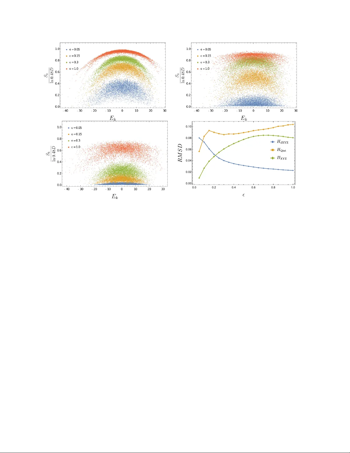
Loading high-quality paper...
Comments & Academic Discussion
Loading comments...
Leave a Comment