Sequential Bayesian Experimental Design for Prediction in Physical Experiments Informed by Computer Models

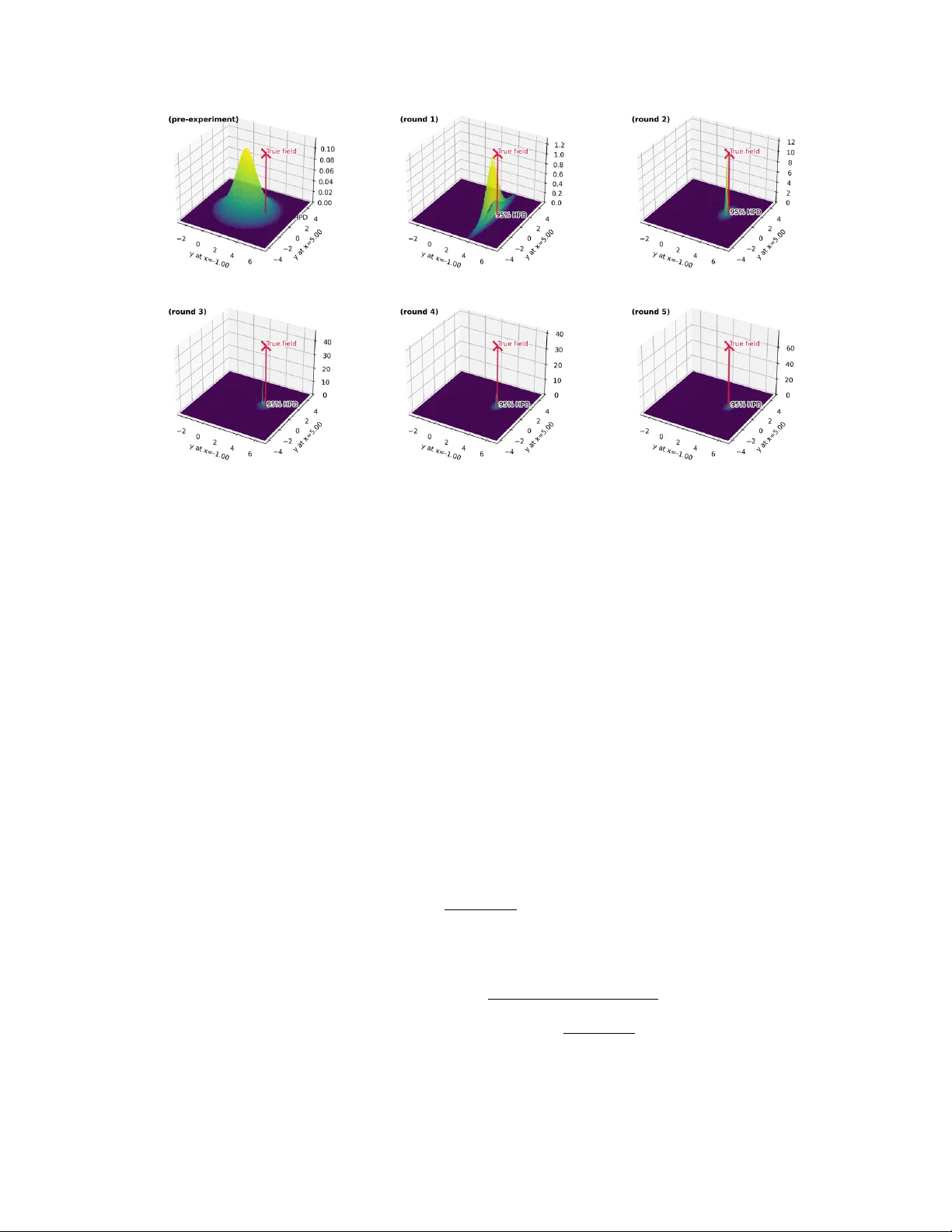
Sequen tial Ba y esian Exp erimen tal Design for Prediction in Ph ysical Exp erimen ts Informed b y Computer Mo dels Hao Zh u ∗ Markus Hain y ∗ Marc h 18, 2026 Abstract In man y scientiﬁc and engineering domains, ph ysical exp erimen ts are often costly , non-replicable, or time-consuming. The Kennedy & O’Hagan (K OH) mo del framew ork has b ecome a widely used approac h for combining sim ulator runs with limited exp er- imen tal observ ations. Under Ba yesian implemen tation, the simulator output, mo del discrepancy , and observ ation noise are jointly mo deled by coupled Gaussian pro cesses, follo wed b y coherent p osterior inference and uncertain ty quan tiﬁcation. This work presen ts a genuinely sequential Ba yesian exp erimen tal design (BED) framework ex- plicitly aimed at improving the predictive p erformance of the K OH mo del. W e employ a m utual information (MI)–based criterion and dev elop a h ybrid v ariant that in tegrates with measures of lo cal mo del complexit y , leading to signiﬁcantly more eﬃcient design decisions. W e further theoretically show that the MI-based criterion is more compre- hensiv e and robust than the classical in tegrated mean squared prediction error (IMSPE) minimization criterion, esp ecially when the model is highly uncertain in the early stages of the exp eriment. T o mitigate the computational burden of the fully Bay esian infer- ence and the ensuing BED pro cess, we propose tw o acceleration strategies—Gaussian Mixture Compression and Sch ur complement & rank-one up date—which together sub- stan tially reduce run time. Finally , we demonstrate the eﬀectiveness of the proposed metho ds through b oth a synthetic example and a real bio c hemical case study , and compare them against sev eral classical design criteria under sequen tial (oﬄine) and adaptiv e (online) BED settings. Keyw ords: Ba y esian exp erimen tal design; Kennedy and O’Hagan mo del; Mutual informa- tion; Sequential design; Gaussian pro cess; lo cal mo del complexity 1 In tro duction In many ﬁelds of science and engineering, computer mo dels serv e as simulators to en- hance the understanding of real-w orld phenomena. They provide abstractions for the actual ph ysical pro cess and v ary in lev el of accuracy . How ever, in many cases, computer mo dels ∗ Institute of Applied Statistics, Johannes Kepler Univ ersit y Linz Corresp onding author email: hao.zhu@jku.at 1 inevitably deviate from the true physical pro cess. Field data consequen tly pla y a crucial role in reﬁning and calibrating computer models, as they correct model errors. Ho wev er, acquir- ing ﬁeld data, either from observ ations or through laboratory experiments, can b e exp ensiv e and challenging. F or instance, the disco v ery of new materials with a sp eciﬁc prop erty often demands a signiﬁcan t num b er of costly and time-consuming experiments ( Dehghannasiri et al. , 2017 ). In these cases, gathering the most informative ﬁeld data through optimal ex- p erimen tal design can signiﬁcantly exp edite the mo deling pro cess and lo w er the cost of the exp erimen t. Sev eral well-established statistical framew orks hav e b een dev elop ed to combine ﬁeld data with simulation data ( Cox et al. , 2001 ; Higdon et al. , 2004 ; Kennedy and O’Hagan , 2001 ). A common feature of these approaches is the use of a computationally cheaper emulator as a surrogate for the exp ensiv e mechanistic mo del. Our w ork builds on the Kennedy and O’Hagan (KOH) framew ork, which enables us to account for m ultiple sources of uncertaint y , including mo del inadequacy and parameter uncertaint y , within a Bay esian setting. Em ula- tors are often constructed using nonparametric metho ds such as Gaussian pro cesses (GPs) ( Rasm ussen and Williams , 2006 ) to capture the highly complex and nonlinear b ehavior of the ph ysical system. Within this framew ork, computer mo dels t ypically inv olv e uncertain inputs which can b e view ed as random v ariables that aﬀect the ov erall sim ulation output. Suc h inputs are referred to as calibration parameters, while others are controllable by the exp erimen ter. A natural wa y to impro v e the p erformance of computer mo dels is through a more accurate calibration of their parameters. Based on this idea, researc hers hav e already prop osed sev eral optimal design metho ds in the K OH framew ork. Pratola et al. ( 2013 ) in tro duced an approach under exp ected im- pro vemen t for sequen tial computer exp erimen ts, similar to the likelihoo d ratio, compar- ing the mo dels with and without the discrepancy term. Huan and Marzouk ( 2013 ) uti- lized information-theoretic metrics to accoun t for parameter uncertain t y and formulated a Ba yesian design for computationally intensiv e mo dels as a contin uous optimization problem. Arendt et al. ( 2015 ), using m ultiv ariate Gaussian sampling, developed a cov ariance-based prep osterior approac h for physical exp eriments. In Krishna et al. ( 2021 ), a h ybrid strategy for ph ysical exp eriments was built: a D-optimal design was used for parameter calibration and a space-ﬁlling design was used for model prediction under the Ba y esian framew ork. More recen tly , Diao et al. ( 2022 ) suggested a sequential D-optimal design metho d for computer mo del calibration and compared its p erformance with other alternatives. S ¨ urer et al. ( 2023 ) selected the exp ected in tegrated v ariance minimization of the calibration parameters as the criterion for sequential Bay esian design, considering the parameter uncertaint y . A common diﬃcult y is that the calibration parameters are typically multiv ariate and confounded with GP h yp erparameters, which results in identiﬁabilit y issues. T o o v ercome this diﬃcult y , Gu and W ang ( 2018 ), W ang et al. ( 2020 ), and Xie and Xu ( 2020 ) introduced pro jection-based metho ds that impro ve the iden tiﬁabilit y of calibration parameters. Nevertheless, computer mo dels still remain imperfect. In other w ords, ev en when all model parameters are accurately iden tiﬁed, systematic/structural mo del inadequacy relative to the true ph ysical pro cess of- ten persists. F or this reason, our w ork fo cuses not on parameter calibration, but on directly impro ving the KOH model’s ov erall predictiv e capability . Indeed, several design criteria targeting ob jectiv es other than parameter calibration hav e also b een prop osed. Ho w ever, little atten tion has b een paid to metho ds that directly target 2 predictiv e p erformance. Among them, Bay arri et al. ( 2007 ) employ ed the Maximin Latin Hyp ercub e Design (LHD) to conduct ﬁeld exp eriments within a fully Bay esian framew ork. Ranjan et al. ( 2011 ) adopted the criterion of maximizing the reduction in the in tegrated mean squared error (IMSE) for physical exp eriments. Williams et al. ( 2011 ) compared several design criteria for sim ulator exp erimen ts, including maximum expected impro vemen t and maxim um entrop y reduction. More recently , Leatherman et al. ( 2017 ) prop osed a joint design strategy that combines the integrated mean squared prediction error (IMSPE) minimization with a nested maximin-augmented LHD to impro ve predictiv e accuracy . Building on this w ork, Ko ermer et al. ( 2024 ) deriv ed a closed-form expression for IMSPE in the K OH mo del framew ork and reformulated it as a contin uous gradient-based optimization problem for computer mo del design. Notably , these approac hes are not information-theoretic and thus diﬀer from fully Bay esian designs that aim to maximize exp ected information gain. When parameter and predictiv e uncertain ties are fully accoun ted for, mutual information gain b ecomes the b est to ol to handle nonlinearity and p oten tial m ultimo dalit y ( Ry an et al. , 2016 ). F urthermore, explicit design methods for ph ysical exp eriments across discrete inputs are largely absent from the literature. Most existing w ork instead targets computer mo del exp erimen ts, where the simulators are assumed to b e operated ov er a contin uous h yp ercub e input space rather than a discrete set of feasible candidate p oints solving the design problem b y using contin uous optimization. Ba yesian exp erimental design (BED) was originally introduced by Lindley ( 1972 ) based on the decision-theoretic approac h, and was later extended by Chaloner and V erdinelli ( 1995 ), who pro vided a comprehensive review and a coherent formulation framew ork applicable to v arious design ob jectives. Higdon et al. ( 2004 ) ﬁrstly developed a fully Bay esian estimation pro cedure for the K OH mo del, enabling an appropriate quantiﬁcation of m ultiple sources of uncertaint y . Most existing Ba y esian design criteria are based on the Kullback–Leibler div ergence b etw een p osterior and prior distributions, commonly referred to as the exp ected information gain (EIG). Ho wev er, the computation of the EIG is notoriously challenging. T o mitigate this problem, recent adv ances ha ve introduced eﬃcient gradien t-based metho ds to optimize the v ariational lo wer b ounds of the EIG ( F oster et al. , 2019 , 2020 ; Kleinegesse and Gutmann , 2021 ). Amortization strategies hav e also gained p opularity in adaptiv e design ( F oster et al. ( 2021 )), where p olicy-based approac hes in deep learning enable one-shot rather than step-b y-step design studies. In line with Bay esian inference under the KOH framew ork, our ob jectiv e is to conduct a BED with minimal simplifying assumptions so that all sources of uncertaint y can b e fully considered. This pap er aims to ﬁll this gap by prop osing a gen- uinely sequen tial BED framework that explicitly fo cuses on designing ph ysical exp eriments across discrete candidate lo cations. The prop osed approach enhances the future predictiv e capabilit y of the K OH mo del o v er successive design rounds and yields more eﬃcien t and robust designs than ad ho c approac hes that neglect certain uncertain ties. This pap er is organized as follo ws. Section 2 reviews the Kennedy & O’Hagan framework, summarizes its Ba yesian implementation, and describ es the design ob jectiv es in this w ork and some existing design criteria under the fully Ba yesian approac h. Section 3 in tro duces the m utual-information–based design criterion, along the extension w e prop ose that incorp orates lo cal predictiv e complexity . Section 4 presen ts a set of strategies that substantially reduce the computational cost of the design. Section 5 ev aluates the p erformance of all criteria considered in this w ork through b oth a syn thetic toy example and a real-w orld dataset. 3 Section 6 concludes with a discussion of the ﬁndings of this pap er and p otential directions for future research. 2 Bac kground and Related W ork In this section, we ﬁrst pro vide a brief review of the K OH framework and its Ba y esian implemen tation. Then, w e in tro duce the design ob jectiv es and give an o v erview of previously emplo yed exp erimen tal design criteria under the Bay esian framework. F urther details are presen ted in the following subsections. 2.1 Review of Kennedy & O’Hagan Mo del W e adopt the computer mo del calibration framework prop osed b y Kennedy and O’Hagan ( 2001 ), along with its subsequen t adaptations for fully Bay esian inference by Higdon et al. ( 2004 ) and Bay arri et al. ( 2007 ). The Kennedy & O’Hagan Mo del, hereafter denoted KOH mo del, is formulated as y p = y c ( X p , θ ) + δ ( X p ) + ϵ , y s = y c ( X c , T ) . Throughout this article, v ectors and matrices are denoted in b oldface. Assume that w e observ e n resp onses from the ph ysical pro cess and m resp onses from the simulator, and let N = n + m b e the total n umber of design p oin ts (ﬁeld + sim ulator). The con trollable design inputs are represen ted by X = ( X c ⊤ , X p ⊤ ) ⊤ = ( x ⊤ 1 , . . . , x ⊤ N ) ⊤ ∈ R N × d , with eac h x i = ( x i 1 , . . . , x id ) ⊤ ∈ R d denoting a single input lo cation. Here, X c and X p corresp ond to the inputs of the computer mo del and the ph ysical exp eriments, resp ectively . Let θ = ( θ 1 , . . . , θ h ) ⊤ ∈ R h b e the v ector of the true calibration parameters and T = ( t ⊤ 1 , . . . , t ⊤ m ) ⊤ ∈ R m × h b e the design setting of the calibration parameters at whic h the sim ulator is ev aluated. The underlying computer model is denoted b y y c ( · , · ), and y s ∈ R m represen ts the simulator outputs ev aluated at a set of design p oin ts X c . Observ ations from the physical pro cess are denoted by y p ∈ R n , with δ ( · ) capturing the discrepancy b etw een the ph ysical pro cess and the computer mo del (for multi-output cases, y p and y s can b e matrix-v alued, with each column corresp onding to one task). The observ ational errors are assumed to b e indep endent and normally distributed as ϵ ∼ N ( 0 , σ 2 I n ), where ϵ = ( ϵ 1 , . . . , ϵ n ) ⊤ ∈ R n . Both y c ( · , · ) and δ ( · ) are mo deled using Gaussian pro cesses (GPs) ( Rasmussen and Williams , 2006 ) under a Ba yesian framew ork. Sp eciﬁcally , the t wo stages can b e formul ated as y c ( X c , T ) ∼ GP  m c ( X c , T ) , K ϕ 1  ( X c , T ) , ( X c ′ , T ′ )   , (1) δ ( X p ) ∼ GP  m δ ( X p ; θ ) , K ϕ 2  X p , X p ′   , (2) where m c ( · , · ) and m δ ( · ; · ) denote the mean functions, and K ϕ 1 ( · , · ) and K ϕ 2 ( · , · ) are the cor- resp onding cov ariance kernels parameterized b y hyperparameters ϕ 1 and ϕ 2 . F or simplicity , w e assume a zero-mean function for the ﬁrst-stage (computer mo del) GP , so m c ( X c , T ) = 0 here. 4 Due to the prop erties of Gaussian pro cesses (GPs), an y ﬁnite collection of outputs fol- lo ws a multiv ariate normal (MVN) distribution. In the K OH mo del, the outputs from the computer mo del and the physical pro cess can b e jointly expressed by a blo ck-structured co v ariance matrix. Sp eciﬁcally , for the observed simulator runs y s and the physical observ a- tions y p , we ha v e y p y s !    θ , ϕ 1 , ϕ 2 , σ 2 ∼ N ( µ , Σ oo ) , (3) where µ =  m δ ( X p ; θ ) , 0 m  ⊤ ∈ R N represen ts the mean and the joint cov ariance matrix Σ oo ∈ R N × N is decomp osed as Σ oo = K c,pp K c,ps K c,sp K c,ss ! | {z } computer GP + K δ,pp 0 0 0 ! | {z } discrepancy GP + σ 2 I n 0 0 0 ! | {z } observ ation noise . Here, K c,pp = K ϕ 1  ( X p , θ ) , ( X p , θ )  ∈ R n × n , K c,ps = K ϕ 1  ( X p , θ ) , ( X c , T )  ∈ R n × m , K c,ss = K ϕ 1  ( X c , T ) , ( X c , T )  ∈ R m × m , K δ,pp = K ϕ 2 ( X p , X p ) ∈ R n × n . F or prediction at a new set of design points X ∗ ∈ R n ∗ × d , w e consider the joint distribution of the future outputs y ∗ and observed data y = ( y p ⊤ , y s ⊤ ) ⊤ : Co v  y ∗ y  = Σ ∗∗ Σ ∗ o Σ o ∗ Σ oo ! ∈ R ( n ∗ + N ) × ( n ∗ + N ) , (4) where Σ ∗∗ = K ϕ 1  ( X ∗ , θ ) , ( X ∗ , θ )  + K ϕ 2 ( X ∗ , X ∗ ) + σ 2 I n ∗ ∈ R n ∗ × n ∗ , Σ ∗ o =  K ϕ 1  ( X ∗ , θ ) , ( X p , θ )  + K ϕ 2 ( X ∗ , X p ) K ϕ 1  ( X ∗ , θ ) , ( X c , T )   ∈ R n ∗ × N , and Σ o ∗ = Σ ⊤ ∗ o . Consequen tly , the predictive distribution of y ∗ conditional on observed data y = ( y p ⊤ , y s ⊤ ) ⊤ is y ∗   y , θ , ϕ 1 , ϕ 2 , σ 2 ∼ N ( µ ∗ , Σ ∗ ) , (5) with predictive mean µ ∗ ∈ R n ∗ and cov ariance Σ ∗ ∈ R n ∗ × n ∗ µ ∗ = m δ ( X ∗ ; θ ) + Σ ∗ o Σ − 1 oo  y − µ  , Σ ∗ = Σ ∗∗ − Σ ∗ o Σ − 1 oo Σ o ∗ . (6) 2.2 Design Ob jectiv es and Strategies Optimal exp erimen tal design t ypically relies on constructing an appropriate design crite- rion or ob jectiv e function. Such a criterion should either directly or indirectly represent the exp ected gain that the exp erimen ter aims to ac hieve. As discussed earlier, the ob jectiv e of this study is to select a set of design p oin ts for physical exp eriments that can improv e the 5 predictiv e p erformance of the K OH mo del accoun ting for all sources of uncertain t y within a BED framework. Compared to computer exp eriments, physical exp eriments are typically constrained by a limited set of candidate p oints and a tight exp erimental budget, which mak es the design problem inherently discrete rather than a con tinuous optimization prob- lem. When real-time exp eriments cannot b e conducted so that the mo del p osterior cannot b e up dated, batc h-optimal design, whic h simultaneously selects all exp erimen tal p oin ts within the given budget b efore the exp erimen ts, in principle p erforms at least as w ell as the se- quen tial greedy approach and often yields b etter p erformance ( M ¨ uller and P¨ otsc her , 1992 ). Ho wev er, as the n umber of candidate p oin ts increases, the com binatorial searc h space grows sup er exponentially , making true batch design computationally infeasible even for mo derate problem sizes. The sequential greedy approach thus serves as a tractable approximation to the batc h-optimal design, providing a practically eﬃcien t and theoretically in terpretable al- ternativ e. Nemhauser et al. ( 1978 ) has established and theoretically prov en a classical result for maximizing a non-negative, monotone submo dular set function under a cardinality con- strain t. Under these conditions, the greedy algorithm can at least achiev e a (1 − 1 /e ≈ 63%) appro ximation to the global optimal v alue. Building on this theorem, Krause et al. ( 2008 ) de- v elop ed a greedy algorithm for sensor placemen t using a mutual-information criterion under a Gaussian pr o cess (GP) model, whic h empirically demonstrates that the greedy strategy can attain near–optimal p erformance. Their setting is closely related to ours, although our fully Ba yesian GP framew ork is more complex and ma y not strictly satisfy the submo dularity or monotonicit y conditions. Ho wev er, the greedy strategy remains a practically eﬀectiv e choice in our setting, as approximate monotonicit y and submo dularity are often suﬃcient for ac hiev- ing high-quality results. In this study , we consider t w o strategies for multi-round Bay esian sequen tial exp erimen tal design: sequen tial (oﬄine) design of exp erimen ts (SDE) and adap- tiv e (online) design of exp erimen ts (ADE). The SDE is actually a greedy approach, seeking the b est lo cation at each round without incorp orating information from future rounds. Supp ose w e ha ve a total budget of B ph ysical exp erimen tal runs. Let D cand = { ξ 1 , . . . , ξ M } denote the ﬁnite set of M candidate lo cations for conducting ph ysical exp eriments, where eac h ξ i ∈ R d represen ts a feasible exp erimental setting in the same input space as X p . Before iteration b , the subset of p oin ts already selected for exp erimen tation is D ( b − 1) sel = { ξ (1) , . . . , ξ ( b − 1) } , and the newly selected p oint in this round is ξ ( b ) ∈ D cand \ D ( b − 1) sel . Af- ter completing all B rounds, the ﬁnal design set is D ( B ) sel = { ξ (1) , . . . , ξ ( B ) } . The predic- tiv e p erformance of the mo del is ev aluated based on the predictiv e results y ∗ at lo cations X pred = X ∗ ∈ R n ∗ × d . Both the sequential design of experiments (SDE) and the adaptiv e design of exp erimen ts (ADE) proceed sequen tially , selecting one new design input at a time according to a speciﬁed design criterion. In SDE, the optimal design input is determined sequentially based on the curren t K OH mo del, without p erforming any physical exp eriment. Consequen tly , the mo del p osterior remains unc hanged throughout the design pro cess. In contrast, ADE conducts real physical exp erimen ts immediately after eac h selected design input. The corresp onding observ ations then update the p osterior b efore the next design input is c hosen. T able 1 clearly illustrates the distinction b et w een the tw o strategies. 6 Algorithm 1 Sequential (SDE) and Adaptive (ADE) Design under the KOH F ramew ork Require: Budget B ; candidates D cand = { ξ 1 , . . . , ξ M } ; prediction set X pred = X ∗ ; initial data { ( X p , X c , y ) } ; mo de ∈ { SDE , ADE } ; criterion or ob jective function Crit ( · ) Ensure: D ( B ) sel = { ξ (1) , . . . , ξ ( B ) } D (0) sel ← ∅ ; ﬁt KOH posterior for b = 1 to B do ξ ( b ) ← arg max(min) ξ ∈D cand \D ( b − 1) sel Crit  ξ ; curren t p osterior , X pred  if mode = SDE then No physical experiment; k eep curren t K OH p osterior unchanged else if mode = ADE then Run exp eriment at ξ ( b ) to get y new ( b ) ; augment data; up date KOH posterior end if D ( b ) sel ← D ( b − 1) sel ∪ { ξ ( b ) } end for return D ( B ) sel and ﬁnal KOH p osterior 2.3 Classical Design Criteria If the ob jective is to directly enhance the future predictive p erformance of the statistical mo del, particularly the KOH model, only a few prior works hav e inv estigated relev ant exper- imen tal design criteria. In practice, space-ﬁlling designs are commonly adopted as an initial exploration and serve as a practical b enc hmark. Beyond that, the IMSPE minimization cri- terion is almost the only measure in the existing literature that directly quantiﬁes predictive uncertain ty . In addition, here we also compare with the D-optimal criterion in this study , whic h fo cuses on improving the estimation of calibration parameters but can also indirectly enhance predictive accuracy . Among these criteria, the D-optimal and IMSPE minimization criteria can actually b e formulated and implemen ted in a fully Bay esian manner, a p ersp ec- tiv e that has b een rarely discussed in previous studies. Their Ba yesian formulations are presen ted in this subsection. In tegrated Mean Squared Prediction Error Minimization The integrated mean squared prediction error (IMSPE) minimization criterion is derived from the I-optimalit y criterion ( Studden , 1977 ), whose purp ose is to maximize the reduction in predictive v ari- ance. It w as initially prop osed by Sac ks et al. ( 1989 ) as a selection criterion for exp erimental p oin ts that minimize the expected predictiv e uncertain ty o ver the input space. Subsequen tly , Leatherman et al. ( 2017 ) and Ko ermer et al. ( 2024 ) provided detailed mathematical form u- lations of IMSPE within the K OH mo del framew ork. Here, w e brieﬂy outline its underlying principle and discuss its implementation in a fully Bay esian approach. Based on the predictive co v ariance matrix given in Equation ( 6 ), the Bay esian form ulation of the IMSPE criterion in this study is given as IMSPE  ξ ( b )  = E Ω ∼ p ( Ω | y )  1 n ∗ tr  Σ ∗ ( X ∗ | y ; Ω , D ( b ) sel )   . (7) 7 where tr( · ) denotes the matrix trace operator. All parameters in the KOH mo del are bundled in to the set Ω = ( θ , ϕ 1 , ϕ 2 , σ 2 ), and p ( Ω | y ) denotes the p osterior distribution. The exp ectation is taken with resp ect to the p osterior distribution of the mo del parameters. In practice, the in tegral is approximated by av eraging with equal w eigh ts 1 /n ∗ o ver the set of predictiv e inputs X pred . W e are lo oking for exp erimen tal designs that minimize the IMSPE, whic h is formally equiv alent to c ho osing ξ ( b ) = arg min ξ ∈D cand \D ( b − 1) sel E Ω ∼ p ( Ω | y )  1 n ∗ tr  Σ ∗ ( X ∗ | y ; Ω , D ( b ) sel )   . In the adaptive (online) design of exp erimen ts (ADE), the p osterior p ( Ω | y ) and the observed resp onse y are b oth updated at eac h round b by the newly selected design input ξ ( b ) and its corresp onding ﬁeld observ ation y new ( b ) . D-optimalit y The K OH mo del framework with t wo-stage GPs yields a closed-form ex- pression for the resp onse likelihoo d. Therefore, we can indirectly aim to impro v e future predictions b y selecting exp erimental designs to b etter estimate calibration parameters θ . According to Krishna et al. ( 2021 ) and Diao et al. ( 2022 ), we can ﬁrst write the Fisher Information Matrix (FIM) of θ in the usual trace form I ij ( θ | Ω ) = ∂ µ ⊤ ∂ θ i Σ − 1 oo ∂ µ ∂ θ j + 1 2 tr  Σ − 1 oo ∂ Σ oo ∂ θ i Σ − 1 oo ∂ Σ oo ∂ θ j  !      Ω , i, j = 1 , . . . , h. (8) Here, µ and Σ oo are inv olved in Equation ( 3 ) and b oth dep end on the parameter set Ω . Th us, the FIM is also conditioned on Ω . In our study , w e w ould like to incorp orate the parameter uncertaint y , thereb y the fully Ba yesian FIM is given as I ij ( θ ) = E Ω ∼ p ( Ω | y ) [ I ij ( θ | Ω )] . The Bay esian D-optimal design is then obtained b y maximizing the log-determinant of the FIM, log det I ij ( θ ), after whic h the corresp onding design input is ξ ( b ) = arg max ξ ∈D cand \D ( b − 1) sel logdet I ij ( θ ) . In sequential (oﬄine) design of exp eriments (SDE), the FIM I ij ( θ ) can still diﬀer across the candidate design inputs ev en though the parameter p osterior p ( Ω | y ) is ﬁxed. This is b ecause adding a new exp erimen tal input expands the mean vector µ and the observ a- tional blo ck of the cov ariance matrix Σ oo , ev en though the p osterior distribution remains unc hanged. In adaptiv e (online) design (ADE), the eﬀect is further ampliﬁed since the pa- rameter p osterior p ( Ω | y ) is also updated when a real ﬁeld resp onse y new ( b ) and a newly selected design input ξ ( b ) are incorp orated. Maximin Distance Under circumstances where prior information of the mo del or exp ert kno wledge is not a v ailable, space-ﬁlling design is commonly adopted ( Johnson et al. , 1990 ; Lin and T ang , 2015 ; Pronzato and M ¨ uller , 2012 ) to seek design p oin ts that ﬁll a b ounded 8 exp erimen tal region as uniformly as p ossible. Johnson et al. ( 1990 ) prop osed the Maximin Distance criterion, which aims to maximize the minimum Euclidean distance b et ween each candidate design p oin t and all previously selected p oin ts. In this study , w e also use it as a geometric b enchmark. The design input is searched in a greedy manner: ξ ( b ) = arg max ξ ∈D cand \D ( b − 1) sel min ξ ( j ) ∈D ( b − 1) sel (1 ≤ j ≤ b − 1)   ξ − ξ ( j ) ∥ 2 . This criterion promotes the space-ﬁlling prop erty of the design without relying on the KOH mo del or any p osterior up dates. Therefore, the decision do es not dep end on whether the design strategy is SDE or ADE. 3 Mutual Information–Based Design Criterion In this section, we in tro duce the bac kground of the con v entional Bay esian exp erimental design (BED) framew ork based on m utual information (MI). Sp eciﬁcally , w e ﬁrst describ e ho w to construct a utilit y function that guides the selection of exp erimental inputs to directly impro ve the predictiv e distribution p ( y ∗ ) (marginalized ov er the mo del parameters Ω ). W e then incorp orate the concept of lo cal complexit y of the mo del prediction and propose a newly hybrid criterion that pro vides a more eﬃcient search for optimal design lo cations. F urthermore, w e in vestigate several theoretical prop erties of the MI-based criterion, including its bias, asymptotic con vergence, and its connection to the IMSPE minimization criterion. 3.1 Mutual Information Gain for Improving F uture Predictions F rom Lindley ( 1972 ), the utility function of BED should hav e the following general form: U ( ξ ) = Z Z u ( ξ , y new ; Ω ) p ( y new , Ω | ξ ) d Ω d y new = Z Z u ( ξ , y new ; Ω ) p ( Ω | y new , ξ ) p ( y new | ξ ) d Ω d y new , (9) where U ( ξ ) is the exp ected utility of the conditional utility function u ( ξ , y new ; Ω ) and y new represen ts the (as yet unobserved) outcome of an exp eriment conducted at ξ . Since the true observ ation is unknown prior to p erforming the exp erimen t, the exp ectation is integrated o ver the join t uncertaint y of the mo del parameters Ω and the p otential observ ation y new . Ry an et al. ( 2016 ) introduced the computation of mutual information (MI) b etw een the v ariable of interest and the p otential observ ation. Consistent with the design ob jective and sequen tial design strategy describ ed in Section 2.2 , the exp ected utility at each round b can b e expressed as U ( ξ ( b ) ) = I ( y ∗ ; y new ( b ) | y , D ( b ) sel ) = Z Z p ( y ∗ | y new ( b ) , y , D ( b ) sel ) p ( y new ( b ) | y , D ( b ) sel ) × log p ( y ∗ | y new ( b ) , y , D ( b ) sel ) p ( y ∗ | y , D ( b ) sel ) d y new ( b ) d y ∗ . (10) 9 Corresp onding to ( 9 ), the marginalized utilit y function ov er Ω is deﬁned as the log ratio b et w een the p osterior and prior predictive distributions of the quan tity of interest: u ( ξ ( b ) , y new ( b ) ; y ∗ ) = log p ( y ∗ | y new ( b ) , y , D ( b ) sel ) p ( y ∗ | y , D ( b ) sel ) . W e are not the ﬁrst to prop ose this utilit y function. Chaloner and V erdinelli ( 1995 ) and Kleinegesse and Gutmann ( 2021 ) also presented similar formulations, although they either ignored parameter uncertaint y or conceptually marginalized it out, thereb y not fully captur- ing ho w this uncertaint y propagates to quan tities y new ( b ) and y ∗ . In this work, w e explicitly expand the marginal distributions to accoun t for the impact of parameter uncertain ty on b oth the p otential observ ation and the future prediction. F or computational con v enience, w e can rewrite Equation ( 10 ) as U ( ξ ( b ) ) = Z Z p ( y ∗ , y new ( b ) | y , D ( b ) sel ) × log p ( y ∗ , y new ( b ) | y , D ( b ) sel ) p ( y new ( b ) | y , D ( b ) sel ) p ( y ∗ | y , D ( b ) sel ) d y new ( b ) d y ∗ . (11) Eac h marginal lik eliho o d term in b oth the numerator and denominator of Equation ( 11 ) is obtained by in tegrating ov er the p osterior distribution of the mo del parameters Ω ), e.g. p ( y ∗ , y new ( b ) | y , D ( b ) sel ) = Z p ( y ∗ , y new ( b ) | Ω , D ( b ) sel ) p ( Ω | y ) d Ω , p ( y new ( b ) | y , D ( b ) sel ) = Z p ( y new ( b ) | Ω , D ( b ) sel ) p ( Ω | y ) d Ω , p ( y ∗ | y , D ( b ) sel ) = Z p ( y ∗ | Ω , D ( b ) sel ) p ( Ω | y ) d Ω . In the adaptive (online) design of exp erimen ts (ADE), the p osterior p ( Ω | y ) and the observed resp onse y are b oth up dated or app ended at each round b . Considering both parameter un- certain ty and predictiv e uncertain ty , this utility function can b e interpreted as the exp ected Kullbac k-Leibler (KL) div ergence ( Kullbac k and Leibler , 1951 ) b etw een the posterior predic- tiv e and prior predictiv e distributions of future observ ations y ∗ , integrated o ver all p ossible mo del parameters Ω . Hence, the design input can b e selected b y maximizing the exp ected utilit y ξ ( b ) = arg max ξ ∈D cand \D ( b − 1) sel U ( ξ ) . Figure 1 sho ws an illustrative example of the ev olution of the join t predictive distribution at tw o lo cations ov er a 5-run sequential (oﬄine) design of exp eriments (SDE) using this prop osed criterion. W e can see from the plot that, as the design rounds progress, the uncertain ty of the distribution decreases substan tially and the p osterior density (95% Highest P osterior Densit y (HPD)) is b ecoming more sharply fo cused around the true v alue. 10 Figure 1: Evolution of the joint predictive distribution at t wo lo cations under a 5-run se- quen tial (oﬄine) design of exp eriments (SDE) using the prop osed MI-based criterion. 3.2 Hybrid Criterion with Lo cal Complexit y Adjustmen t The criterion based on mutual information gain prop osed abov e can help obtain the p oin ts that yield the greatest reduction in global predictiv e uncertaint y . Ho wev er, this criterion may also ha ve the drawbac k of ov ersampling in regions of high predictive v ariance and missing critical mo del structure such as extrema or inﬂection regions. Inspired b y n umerical optimization methods such as Newton’s metho d ( Bonnans et al. , 2006 ), w e prop ose to quan tify the lo cal complexity of the predictiv e surface through a comp osite metric that com bines the lo cal slop e and the slop e-v ariation at the candidate input ξ ( b ) . Let the predictive mean function at a single candidate input ξ ( b ) ∈ R d b e expressed as µ ∗ ( ξ ( b ) ) ∈ R p , where p denotes the num b er of output dimensions (tasks). In a fully Bay esian w ay it can b e written as µ ∗ ( ξ ( b ) ) = E Ω ∼ p ( Ω | y )  µ ∗ ( ξ ( b ) ; Ω )  . The lo cal slop e at ξ ( b ) is then characterized b y the Jacobian matrix J ( ξ ( b ) ) = ∂ µ ∗ ( ξ ( b ) ) ∂ ξ ( b ) ∈ R p × d , whose F rob enius norm quantiﬁes the o verall rate of change of the predictive mean ﬁeld with resp ect to the input dimensions: g ( ξ ( b ) ) = ∥ J ( ξ ( b ) ) ∥ F = v u u t p X i =1 d X j =1  ∂ µ ∗ i ( ξ ( b ) ) ∂ ξ ( b ) ,j  2 , (12) where ξ ( b ) =  ξ ( b ) , 1 , ξ ( b ) , 2 , . . . , ξ ( b ) ,d  ⊤ . In practice, we ﬂatten all outputs into a single vector so that the m ulti-task case can b e treated as a single-output scenario and F rob enius norm 11 pro vides a natural scalar measure of lo cal sensitivity without requiring task-speciﬁc w eights. The scalar quan tit y g ( ξ ( b ) ) serves as a measure of the local slope or steepness of the predictive mean ﬁeld, and forms the ﬁrst comp onent of our comp osite lo cal complexit y metric. The other comp onen t of the metric ev aluates the c hange rate of the lo cal slope. In contin- uous optimization problems, this can b e conv enien tly quantiﬁed using curv ature. How ev er, in the context of ph ysical exp erimental design, where the budget is normally limited and the candidate design inputs are highly discrete, it is impractical to compute smo oth deriv atives. Therefore, w e construct a slop e-c hange score that measures the total v ariation of the lo cal slop e among all discrete candidate p oin ts. Sp eciﬁcally , w e deﬁne it as s ( ξ ( b ) ) = 1 k X j ∈N ( b )   g ( ξ ( b )) − g ( ξ ( j ))   , (13) where N ( b ) denotes the index set of the k nearest neighbors of ξ ( b ) in the input space. This form ulation can b e in terpreted as a discrete analogue of curv ature, measuring ho w rapidly the lo cal slop e changes in the neigh b orho o d of each candidate ξ ( b ). A larger s ( ξ ( b ) ) indicates a region with higher nonlinearity or stronger lo cal v ariation. F or the computation of Equation ( 12 ), either automatic diﬀerentiation or the ﬁnite- diﬀerence method can be employ ed. After obtaining b oth the slop e g ( ξ ( b ) ) from Equation ( 12 ) and the slop e-c hange score s ( ξ ( b ) ) from Equation ( 13 ), we standardize them to the [0 , 1] range and giv e the lo cal complexity measuremen t as a weigh ted com bination of these tw o comp onen ts: C ( ξ ( b ) ) = w g ˜ g ( ξ ( b ) ) + w s ˜ s ( ξ ( b ) ) , w g + w s = 1 , where ˜ g ( · ) and ˜ s ( · ) denote the normalized slop e and slop e-c hange score, resp ectively . The w eights w g and w s can b e freely chosen according to prior knowledge about the mo del b eha vior or diﬀerent design preferences. F or example, a larger w g places more emphasis on regions of steep gradients, while a larger w s encourages exploration of regions exhibiting strong nonlinearity or ﬂuctuation. This comp osite score C ( ξ ( b ) ) therefore oﬀers a ﬂexible and interpretable metric for quan tifying the lo cal complexit y of the mo del. If we hybridize the prop osed lo cal complexit y adjustment with criteria driv en by uncer- tain ty reduction, then we comprehensively account for the global predictive uncertaint y as w ell as the lo cal structural pattern of the predictive surface. Sp eciﬁcally , we can incorp orate the lo cal complexit y term with b oth the MI-based utility in Equation ( 11 ) and the IMSPE in Equation ( 7 ). The formulations of eac h are given b y: U MI hyb  ξ ( b )  = (1 − α ) U  ξ ( b )  + α C  ξ ( b )  , α ∈ [0 , 1] , (14) U IMSPE hyb  ξ ( b )  = (1 − α )  − IMSPE  ξ ( b )  + α C  ξ ( b )  , α ∈ [0 , 1] . (15) The w eighting factor α is also user-chosen to balance the design preference b et ween predictiv e uncertain ty and the lo cal pattern of the predictiv e surface. 3.3 Theoretical Prop erties In Section 2.3 , w e discussed the IMSPE minimization criterion, whic h has a close resem- blance, in terms of function, to the MI-based criterion deﬁned in Equation ( 10 ), as b oth aim 12 to directly reduce predictive uncertaint y . It is therefore theoretically v aluable to formalize the connection b et ween these tw o design ob jectiv es. F or theoretical clarity , we ﬁrst establish the relationship conditional on the mo del parameters Ω . Since the Bay esian design crite- ria considered in this work marginalize ov er Ω through the p osterior distribution p ( Ω | y ), the conditional result can b e in terpreted as describing the lo cal b eha vior of the integrand within the Bay esian exp ectation. In a my opic sequen tial or adaptiv e design framew ork, the selection of the design p oint ξ ( b ) at round b dep ends on the p osterior state obtained after the previous selection ξ ( b − 1) . The MI-based criterion can b e interpreted as quan tifying the c hange in predictive entrop y b efore and after the inclusion of the new observ ation y new ( b ) at ξ ( b ) . While the IMSPE minimization is form ulated in terms of the predictive v ariance at the curren t round b , it implicitly measures the reduction in predictiv e v ariance relativ e to the v ariance obtained from the previous design history D ( b − 1) sel without c ho osing ξ ( b ) . Building on this, w e can provide a general relationship sho wing that the MI-based criterion is lo cally asymptotically equiv alen t to the IMSPE minimization criterion as the sequential design pro- ceeds. W e ma y further in terpret the IMSPE minimization criterion as a relaxed form of the MI-based criterion. It preserv es the same optimization direction but provides a computa- tionally simpler surrogate, since the IMSPE dep ends only on the second moment (trace) of the predictive cov ariance rather than the full cov ariance structure. Before pro ceeding with the formal expression, we denote Σ ∗ ( b − 1) as the pre-exp eriment predictiv e cov ariance matrix at round b − 1, corresp onding to the part Σ ∗ | y ; Ω , D ( b − 1) sel in Equation ( 7 ). Similarly , Σ ∗ ( b ) denotes the corresp onding predictive cov ariance matrix at round b . Let λ min ( Σ ∗ ( b − 1) ) and λ max ( Σ ∗ ( b − 1) ) denote the smallest and the biggest eigen v alue of Σ ∗ ( b − 1) , resp ectively . Then, w e ha v e the following theorem: Theorem 1 (Lo cal asymptotic relationship betw een MI and IMSPE) . Assume that, (i) c onditional on Ω , ( y ∗ , y new ( b ) ) is jointly Gaussian, (ii) Σ ∗ ( b − 1) is symmetric p ositive deﬁnite with eigenvalues 0 < λ min ≤ λ max < ∞ . Deﬁne the c ovarianc e r e duction and IMSPE r e duction at r ound b as ∆ Σ ∗ ( ξ ( b ) ) := Σ ∗ ( b − 1) − Σ ∗ ( b ) ⪰ 0 , ∆IMSPE( ξ ( b ) | Ω ) := 1 n ∗ tr  ∆ Σ ∗ ( ξ ( b ) )  , As the se quential design r ounds pr o c e e d, the fol lowing smal l-up date r e gime holds:   ( Σ ∗ ( b − 1) ) − 1 / 2 ∆ Σ ∗ ( ξ ( b ) ) ( Σ ∗ ( b − 1) ) − 1 / 2   2 − → 0 . Then ther e exists a ﬁnite c onstant C b − 1 , dep ending on Σ ∗ ( b − 1) , such that U ( ξ ( b ) | Ω ) ∆IMSPE( ξ ( b ) | Ω ) − → C b − 1 as ∆ Σ ∗ ( ξ ( b ) ) → 0 , and this c onstant is b ounde d in terms of the eigenvalues of Σ ∗ ( b − 1) : n ∗ 2 λ max  Σ ∗ ( b − 1)  ≤ C b − 1 ≤ n ∗ 2 λ min  Σ ∗ ( b − 1)  . Pr o of. See App endix A . 13 This result establishes a quan titative link b et ween the tw o prediction-improv emen t cri- teria. A t each design round, the new chosen lo cation ξ ( b ) and the new observ ation y new ( b ) (if in ADE) bring a reduction to predictiv e cov ariance. As the rounds pro ceed sequentially and b b ecomes suﬃcien tly large, maximizing m utual information b ecomes asymptotically equiv alent to minimizing the IMSPE, with their diﬀerence collapsing to a ratio factor only related to the current predictiv e uncertaint y structure. This ratio factor can b e stable as the predictiv e cov ariance matrix b ecomes approximately isotropic as the design rounds contin ue, leading to the limiting equiv alence established in Theorem 1 . The theorem is stated condi- tional on the mo del parameters Ω , ho wev er, the Ba yesian design criterion marginalizes o ver Ω through the p osterior p ( Ω | y ). As the sequen tial design progresses, the p osterior up date of Ω also b ecomes increasingly small, i.e., p ( Ω | y 1: b ) − p ( Ω | y 1: b − 1 ) → 0, the conditional asymptotic equiv alence extends naturally to the Bay esian (marginalized) setting. F rom another p ersp ective, the MI-based criterion can b e in terpreted as a sp ectrally w eighted v ersion of IMSPE. In early design stages, when b is relativ ely small and predictiv e uncertain ty is highly anisotropic, the MI-based criterion is more sensitiv e to the directions asso ciated with larger uncertaint y reduction and it can guide exp erimental design more ef- fectiv ely esp ecially at early rounds. Therefore, the MI-based criterion can b e regarded as a generalization of the IMSPE criterion, providing enhanced robustness and exploration abilit y . This is more aligned with the Ba y esian exp erimental design framew ork b ecause it explicitly considers the full structure of predictiv e cov ariance throughout the pro cess. F or the computation of m utual information gain in Equation ( 11 ), due to the intractabilit y of the marginal lik eliho o d of y ∗ and y new ( b ) b oth individually and jointly—as w ell as the p osterior p ( Ω | y ), the con ven tional Mon te Carlo (MC) estimator cannot be directly applied. Instead, a nested Mon te Carlo (NMC) estimator ( Rainforth et al. , 2018 ) is required. In particular, ( 11 ) can b e computed as an NMC estimator: b U S,J ( ξ ( b ) ) = 1 S S X s =1 " log b p joint J  y ∗ s , y new ( b ) ,s  − log b p ∗ J  y ∗ s  − log b p new J  y new ( b ) ,s  # . (16) Let S ∈ N b e the num b er of outer samples and J ∈ N the n um b er of inner samples. F or each outer index s = 1 , . . . , S , w e ﬁrst dra w Ω (0) s ∼ p ( Ω | y , D ( b ) sel ) and then sample ( y ∗ s , y new ( b ) ,s ) ∼ p ( y ∗ , y new ( b ) | y , Ω (0) s , D ( b ) sel ). In the inner lay er, we indep endently dra w Ω (1: J ) s = { Ω ( j ) s } J j =1 i.i.d. from p ( Ω | y ). The Monte Carlo estimates of each corresp onding marginal densit y in Equation ( 16 ) for eac h outer sample s can then b e expressed as b p joint J  y ∗ s , y new ( b ) ,s  = 1 J J X j =1 p  y ∗ s , y new ( b ) ,s | Ω ( j ) s , D ( b ) sel  , b p ∗ J  y ∗ s  = 1 J J X j =1 p  y ∗ s | Ω ( j ) s , D ( b ) sel  , b p new J  y new ( b ) ,s  = 1 J J X j =1 p  y new ( b ) ,s | Ω ( j ) s , D ( b ) sel  . 14 W e now examine the asymptotic behavior of the prop osed NMC estimator b U S,J ( ξ ( b ) ) to wards U ( ξ ( b ) ) as the n umber of samples increases. F rom Hong and Juneja ( 2009 ), if the outer- la yer transformation/function is thrice diﬀerentiable with b ounded third deriv ative, then the estimator can ac hiev e a con v ergence rate of O (1 /S + 1 /J 2 ). Here in our setting, the transformation is f ( · ) = log ( · ), thus it satisﬁes these smoothness conditions on an y compact subset [ τ , ∞ ) ⊂ R + , as summarized in the lemma b elow. Lemma 1 (Smo othness and b ounded deriv ativ es of the outer-lay er function) . L et the outer- layer function of the pr op ose d NMC estimator b e the lo g function f : R + → R , x 7→ log ( x ) . L et the ar gument of f b e lower-b ounde d by a suﬃciently smal l p ositive c onstant τ > 0 , i.e., f is only evaluate d for inputs in [ τ , ∞ ) . Then f is thric e diﬀer entiable c ontinuously on [ τ , ∞ ) , and al l derivatives up to or der thr e e ar e b ounde d. Pr o of. See App endix A . F ollowing Lemma 1 , our MI-based utilit y function can b e view ed as a sp eciﬁc instance of the general nested exp ectation problem analyzed by Hong and Juneja ( 2009 ). Therefore, the NMC estimator in Equation ( 16 ) satisﬁes the established con vergence prop erties, with the mean square error of b U S,J ( ξ ( b ) ) decaying at a rate of O (1 /S + 1 /J 2 ). Corollary 1 (Conv ergence of the NMC estimator) . Under the c onditions in L emma 1 and assuming indep endenc e b etwe en the inner and outer samplers, the me an squar e d err or of b U S,J ( ξ ( b ) ) c onver ges to 0 at r ate O ( S − 1 + J − 2 ) , E  ( b U S,J ( ξ ( b ) ) − U ( ξ ( b ) )) 2  = O ( S − 1 + J − 2 ) . Pr o of. See App endix A . If the total computational budget is T = S × J , Rainforth et al. ( 2018 ) show ed that the NMC estimator can ac hieve its optimal conv ergence rate of the tightest b ound O ( T − 2 / 3 ) when the inner sample size J is prop ortional to S 2 . It is also known that the NMC estimator is biased for any ﬁnite J , while increasing the outer sample size S → ∞ can merely eliminate the v ariance. How ever, if J → ∞ additionally , the NMC estimator in our work con verges almost surely to the true utility v alue b ecause the bias term is also eliminated. Corollary 2 (Bias and almost sure conv ergence of the NMC estimator) . F or any ﬁnite S , J , b U S,J ( ξ ( b ) ) is a biase d estimator of U ( ξ ( b ) ) , i.e., E [ b U S,J ( ξ ( b ) )]  = U ( ξ ( b ) ) . Under the r e gularity c onditions of L emma 1 , if J → ∞ and S → ∞ , then b U S,J ( ξ ( b ) ) c onver ges to U ( ξ ( b ) ) almost sur ely: b U S,J ( ξ ( b ) ) a.s. − − → U ( ξ ( b ) ) . Pr o of. See App endix A . 15 4 Computation Strategies After discussing the prop osed MI-based criterion in Section 3.1 and the classical criteria in Section 2.3 , w e now presen t sev eral computational strategies aimed at reducing the o v erall computational cost and demonstrating the resulting eﬃciency gains. In Section 3.3 , w e discussed that the computational burden of the NMC estimator for the MI-based criterion is substantial as it requires tw o lay ers of discretized in tegration. Sp eciﬁcally , w e sample the predictive resp onse y ∗ and y new ( b ) as w ell as the mo del parameters Ω in order to consider all sources of uncertaint y . The outer sample size S primarily determines the magnitude of the predictive v ariance and t ypically dep ends on the dimensionality of the conditional Gaussian distribution p ( y ∗ s , y new ( b ) ,s | Ω ( j ) s , D ( b ) sel ). According to Corollary 1 and Corollary 2 , the estimate b U S,J ( ξ ( b ) ) b ecomes accurate as J → ∞ and S → ∞ . When using exp erimental design criteria based on computing the cov ariance matrix, reducing S is generally impractical, as doing so would inevitably result in high Mon te Carlo v ariance and unstable design decisions. In contrast, the required inner sample size J largely dep ends on the complexit y of the p osterior distribution p ( Ω | y ). Th us, it is more desirable to reduce J , which corresp onds to constructing a reﬁned appro ximation using few er comp onen ts in the asso ciated Gaussian mixture, even though this pro cedure ma y in tro duce some extra bias, depending on ho w m uc h representational capacity is retained. Other than existing approac hes that use the v ariational low er b ounds to appro ximate the real EIG by sto chastic gradien t descen t ( F oster et al. , 2019 , 2020 ; Kleinegesse and Gutmann , 2021 ), our metho d is motiv ated by Runnalls’ algorithm ( Runnalls , 2007 ) and clustering-based reduction metho ds ( Sc hieferdeck er and Hub er , 2009 ). W e mitigate the computational cost b y compressing the Gaussian mixture, whic h is the inner la yer of the NMC estimator in Equation ( 16 ), enabling a substantial reduction in computational cost while preserving the representational capacity as muc h as p ossible. In Algorithm 1 , if w e p erform online adaptiv e design of exp eriments (ADE), the p oste- rior distribution p ( Ω | y ) m ust b e up dated after each exp eriment b y app ending the newly observ ed resp onse y new ( b ) to the existing data y . Consequen tly , the predictive quantities µ ∗ and Σ ∗ in Equation ( 6 ) m ust also b e up dated at every round. In contrast, under oﬄine se- quen tial design of exp eriments (SDE), the parameter p osterior remains ﬁxed b ecause no real exp erimen ts are p erformed during the design stage. Thus, the predictiv e mean µ ∗ remains unc hanged across rounds. Ho wev er, the predictive cov ariance Σ ∗ still v aries b ecause the co- v ariance structure dep ends not only on the parameters Ω but also on the relative p ositions of the inputs. Therefore, for criteria in v olving cov ariance computations, such as IMSPE minimization, D-optimality , and mutual information gain, the naiv e implementation would require recomputing the predictive co v ariance from scratch at each round. T o address this issue and accelerate the SDE pro cess , w e precompute and cac he the full cov ariance matrix in the b eginning, and then apply the Sch ur complemen t up dates to obtain the predictive co v ariance eﬃciently . 4.1 Gaussian Mixture Compression W e ﬁrst brieﬂy o verview Runnalls’ algorithm. Runnalls’ metho d ( Runnalls , 2007 ) re- duced the Gaussian mixture mo del (GMM) b y greedily pruning or merging comp onen ts so 16 as to minimize the increase in Kullback-Leibler (KL) divergence. At eac h iteration, the al- gorithm ev aluates and compares the divergence for all candidate pairs, merges the optimal pair via moment matching, and rep eats this process until the desired num b er of comp onents is reac hed. It is commonly used as an initiation for mixture reduction. In addition, the k -means algorithm ( Lloyd , 1982 ) is a classical clustering metho d frequen tly emplo yed for classifying high-dimensional data. Unlik e the approac h of Schieferdec k er and Hub er ( 2009 ), whic h ﬁrst applies Runnalls’ algorithm, then performs k -means clustering, follow ed by a reﬁnemen t step, our metho d is more appropriate to high-dimensional Gaussian mixtures. Because the predictive outputs often in volv e dozens or ev en hundreds of lo cations, it is es- sen tial to normalize the comp onent means b efore p erforming clustering. As the ﬁrst step, w e whiten the conditional prediction using the Cholesky decomp osition of Σ ∗ avg = E [ Σ ∗ j ] + Cov( µ ∗ j ) , j = 1 , . . . , J whic h can b e in terpreted as a combination of the av erage co v ariance and the disp ersion of the predictiv e means. This measure ensures that all directions are scaled comparably , and thus Euclidean distances in the transformed space more faithfully reﬂect Mahalanobis distances. F or simplicit y , w e omit the outer sample index here and denote the whitened means u ∗ j b y u ∗ j = L − 1 ( µ ∗ j − ¯ µ ∗ ) , LL ⊤ = Σ ∗ avg , j = 1 , . . . , J. In the second step, w e apply k -means clustering in this whitened space to compress the original J comp onents in to an initially smaller represen tation with J 0 clusters. F or eac h cluster, moment matc hing (mean and co v ariance) is p erformed to obtain a reduced GMM with J 0 comp onen ts. Each comp onent is characterized by a new mean µ ⋆ k , cov ariance Σ ⋆ k , and weigh t π ⋆ k ( k = 1 , . . . , J 0 , π k ≥ 0 , P k π k = 1). Next, w e reﬁne the mixture of J 0 initial clusters b y applying a greedy Runnalls’ algorithm to further reduce the num b er of comp onents to a target v alue J target . T o improv e stabilit y and reduce computational ov erhead, w e precompute the Cholesky factors and log-determinan ts of all co v ariance matrices prior to this step. The loss function is based on the KL div ergence, and in our case is given as D ij = 1 2 h ( π i + π j ) log | Σ ⋆ ij | − π i log | Σ ⋆ i | − π j log | Σ ⋆ j | i . where Σ ⋆ ij is the co v ariance matrix obtained via momen t matc hing b et ween comp onents i and j among J 0 comp onen ts. How ev er, computing momen t matc hing for all pairwise com binations (random pairing) requires O ( J 2 0 ) op erations, whic h could b e very exp ensive in practice b ecause complex p osterior distributions usually require very large sample sizes J and hence large J 0 . T o o vercome this limitation, we consider a key innov ation: using K-nearest neighbors (KNN) ( Co v er and Hart , 1967 ) to restrict candidate merging pairs. After whitening, the scales across diﬀerent directions b ecome consisten t, and the Euclidean distance b etw een tw o Gaussian distributions b ecomes more aligned with a Mahalanobis geometry . Consequently , the nearest neighbors of a comp onen t are almost alw ays the most promising candidates for merging, whic h av oids unnecessary global pairwise comparisons. By selecting nn k nearest neighbors p er comp onent, the computational complexity is reduced from O ( J 2 0 ) to O ( J 0 × nn k ) and the reduced mixture still retains the strong representational capacit y of the original GMM. The pro cess is summarized in Algorithm 2 . 17 Algorithm 2 Gaussian Mixture Compression with Whitening, k -means Initialization, and KNN-Guided Runnalls Require: Original mixture { ( π j , µ ∗ j , Σ ∗ j ) } J j =1 (equal w eights in MCMC case: π j = 1 /J ); ﬁnal target size J target ; initial cluster size J 0 ; KNN size nn k ; refresh p erio d r Ensure: Compressed mixture { ( π ⋆ k , µ ⋆ k , Σ ⋆ k ) } J target k =1 Whitening. Compute ¯ µ ∗ = 1 J P j µ ∗ j and Σ ∗ avg ≈ 1 J P j Σ ∗ j + 1 J P j ( µ ∗ j − ¯ µ ∗ )( µ ∗ j − ¯ µ ∗ ) ⊤ . Cholesky decomp osition: LL ⊤ = Σ ∗ avg . Whiten means: u ∗ j = L − 1 ( µ ∗ j − ¯ µ ∗ ). k -means compression. Run w eighted k -means on { u ∗ j } to obtain J 0 clusters; for eac h cluster p erform moment matc hing to form new comp onents { ( π ⋆ k , µ ⋆ k , Σ ⋆ k ) } J 0 k =1 . KNN construction. Re-whiten the J 0 new comp onen ts obtained from the last stage and build KNN neighborho o ds of size nn k . KL-based merging. F or each KNN pair ( i, j ) use Runnalls’ algorithm based on D ij = 1 2  ( π ⋆ i + π ⋆ j ) log | Σ ⋆ ij | − π ⋆ i log | Σ ⋆ i | − π ⋆ j log | Σ ⋆ j |  . After it, we obtain the moment-matc hed merge ( π ⋆ ij , µ ⋆ ij , Σ ⋆ ij ). while J 0 > J target do Ev aluate D ij o ver KNN pairs and merge ( i, j ) = arg min D ij . Up date ( π ⋆ k , µ ⋆ k , Σ ⋆ k ) using moment matc hing. Ev ery r merges: re-whiten and rebuild the KNN neighborho o ds. end while return Final compressed mixture { ( π ⋆ k , µ ⋆ k , Σ ⋆ k ) } J target k =1 . 18 4.2 Precomputation and Sch ur Complemen t W e consider the enlarged co v ariance structure after the ﬁrst b design p oints hav e b een selected. Then, unlike the original full cov ariance matrix in Equation ( 4 ), the up dated one at round b is Co v     y ∗ y new (1: b ) y     =    Σ ∗∗ Σ ∗ (new , 1: b ) Σ ∗ o Σ (new , 1: b ) ∗ Σ (new , 1: b ) (new , 1: b ) Σ (new , 1: b ) o Σ o ∗ Σ o (new , 1: b ) Σ oo    ∈ R ( n ∗ + N o ) × ( n ∗ + N o ) , where N o = n + m + b and we can extract the observ ational blo ck p ortion out of this matrix and deﬁne it b y Σ ( b ) oo := Σ (new , 1: b ) (new , 1: b ) Σ (new , 1: b ) o Σ o (new , 1: b ) Σ oo ! ∈ R N o × N o . F or the IMSPE minimization criterion and MI-based criterion, the core part of computation in volv es ev aluating the predictive cov ariance Σ ∗ via Equation ( 6 ). Inside this form ula, we can recognize the computational b ottleneck is the inv ersion of the observ ation blo c k Σ ( b ) oo . In the sequential exp erimental design, Σ ( b ) oo expands to Σ ( b +1) oo and must in principle b e in verted at every round, resulting in substantial computational cost. If w e directly rely on Gaussian pro cess prediction APIs to compute Σ ∗ , we ha v e to reconstruct and inv ert the enlarged kernel matrix at each round. F or each Ω ( j ) s , each round b and eac h candidate design p oin t ξ ∈ D cand \ D ( b − 1) sel , the computational complexit y therefore is O  N 3 o + N 2 o n ∗ + N o n ∗ 2  , where N 3 o stands for Cholesky decomp osition of Σ ( b ) oo and the other tw o terms corresp ond to t wo triangular solv es, thus the ﬁnal complexity is dominated b y the relative sizes of N o and n ∗ . T o reduce this computational burden, w e prop ose a metho d that ﬁrst precomputes the full co v ariance matrix o v er all observ ations, candidate p oin ts, and prediction inputs. A t each round, the corresp onding submatrix required by the criterion is then obtained b y slicing the precomputed kernel matrix according to the selected design lo cation. In this w ay , all co v ariance blo cks needed can b e obtained via inexp ensive slicing instead of recomputation. Since the cov ariance structure expands by adding one input at each round, we apply the eﬃcien t Sch ur complement together with a rank-one up date ( Sherman and Morrison , 1950 ) to up date the required matrices. This av oids recomputing the full in verse  Σ ( b ) oo  − 1 at each round as well as the corresp onding predictiv e co v ariance Σ ∗ ( b ) . As a result, the computational complexit y is decreased from cubic to quadratic, b eing O  N 2 o + N o n ∗ + n ∗ 2  , and similarly the complexit y is dominated b y the relative sizes of N o and n ∗ . The computa- tional details can b e seen in App endix B . 19 4.3 Ov erall Computational Complexit y W e no w summarize the ov erall computational savings in ev aluating the predictiv e co- v ariance Σ ∗ in a fully Bay esian approac h, achiev ed b y com bining the Gaussian mixture compression in Section 4.1 with the precomputation and Sc hur complement strategy in Sec- tion 4.2 . Firstly , let us ﬁgure out the total ev aluations ov er all candidate design p oints in D cand across the budget B rounds in SDE. The set D cand con tains M initial candidates. Let D ( b − 1) sel denote the set of selected design p oints after ( b − 1) rounds. A t round b , the num b er of remaining candidates is M b =   D cand \ D ( b − 1) sel   = M − ( b − 1) . Hence, the total n umber of scans o ver the entire sequential design can b e expressed by B X b =1 M b = B X b =1  M − b + 1  = M B − B ( B − 1) 2 . F or notational brevity , we let the complexity of this part b e O ( B M ). Naiv e baseline. If we compute Σ ∗ ( b ) without an y compression or precomputation, the naive o verall complexit y can therefore b e given as O  J × B M | {z } total candidates ov er all rounds × ( N 3 o + N 2 o n ∗ + N o n ∗ 2 )  . After impro vemen t. Com bining b oth impro v ements in Section 4.1 and Section 4.2 , the o verall complexit y b ecomes O  J target × B M | {z } total candidates ov er all rounds × ( N 2 o + N o n ∗ + n ∗ 2 )  . In comparison, it is evident that combining the tw o strategies yields substan tial compu- tational sa vings, esp ecially for the eﬃciency of the MI-based, IMSPE minimization and D-optimal criteria. Complexit y of diﬀerent design criteria. Having established the cost of computing the predictiv e co v ariance Σ ∗ in the fully Bay esian setting, w e no w turn to the three design criteria in tro duced earlier. These three all depend on the computation of the cov ariance matrix but diﬀer in additional w ork due to their resp ective utilit y functions. 1. Mutual information (MI) gain : The MI-based criterion requires S outer samplers to compute the log-density of a joint Gaussian distribution of dimension ( n ∗ + 1) and J target Gaussian mixture comp onen ts. Each Gaussian log-densit y ev aluation requires only one triangular solve and one quadratic form, th us the complexity is O (( n ∗ + 1) 2 ). Therefore, the total complexit y for the MI criterion b ecomes O  J target × B M × ( N 2 o + N o n ∗ + n ∗ 2 ) + S × J target × B M × ( n ∗ + 1) 2  , assuming that one new design input is selected at each round. 20 2. IMSPE minimization : Compared with MI, the IMSPE minimization criterion in the Bay esian setting only requires computing the trace of Σ ∗ ( b ) for each Ω ( j ) sample and do es not inv olve the outer S -lo op. It is already computationally eﬃcient, but with our Gaussian mixture compression strategy , the ov erall complexity reduces to O  J target × B M × ( N 2 o + N o n ∗ + n ∗ 2 )  . 3. D-optimalit y : The fully Ba yesian D-optimal criterion is diﬀerent from the t w o crite- ria ab ov e in that it relies primarily on the observ ation cov ariance blo ck Σ ( b ) oo and the predictiv e mean µ ( b ) in Equation ( 8 ). While the up date of  Σ ( b ) oo  − 1 can b e accelerated b y using the Sc hur complement as introduced in Section 4.2 , ev aluating the Fisher information matrix for each θ ( j ) = ( θ ( j ) 1 , . . . , θ ( j ) h ) still requires ﬁnite-diﬀerence ev alua- tions of ∂ θ i µ and ∂ θ i Σ oo , and h 2 trace terms. The ﬁnal computational complexit y is O ( h 2 × N 2 0 ) since the FIM is of size ∈ R h × h . Therefore the total complexit y can b e written as O  J × B M × h 2 × N 2 0  , whic h ma y b e signiﬁcantly higher than the complexit y of the IMSPE or MI criteria when h is large. 5 Exp erimen ts In this section, we ev aluate and compare the p erformance of the MI-based criterion—together with its h ybrid v ariant incorp orating lo cal complexity introduced in Section 3 —with several classical criteria describ ed in Section 2.3 through simulation studies. W e presen t one nu- merical toy example and one real-world case study to compare all metho ds in terms of (i) predictiv e accuracy , (ii) uncertain ty quan tiﬁcation, and (iii) design time. T o this end, we emplo y t wo ev aluation metrics. In the formulas b elow, we only discuss one-dimensional out- puts, while for multi-task cases the results can b e obtained by av eraging across the output dimensions. 5.1 Ev aluation Criteria T o assess the predictive p erformance of the mo del after exp erimen ts using the prop osed design metho ds, we consider tw o ev aluation criteria that measure diﬀerent aspects of predic- tion qualit y . The mean squared error (MSE) ev aluates the accuracy of the predictiv e mean, while the contin uous ranked probability score (CRPS) helps accoun t for the predictive un- certain ty . • Mean Squared Error (MSE). Giv en J p osterior samples of parameters { Ω ( j ) } J j =1 , the j -th p osterior predictive mean at lo cations X pred = X ∗ ∈ R n ∗ × d is obtained from ( 6 ) as µ ∗ j = µ ∗ j ( X ∗ ) ∈ R n ∗ . The Bay esian predictive mean is taking the av erage ov er the J p osterior samples ¯ µ ∗ = 1 J J X j =1 µ ∗ j . 21 The true v alues on the predictiv e lo cations are y ∗ ∈ R n ∗ , hence we can deﬁne the predictiv e mean squared error (MSE) in the Bay esian setting as MSE = ∥ ¯ µ ∗ − y ∗ ∥ 2 F , where ∥ · ∥ F denotes the F rob enius norm. • Con tin uous Rank ed Probabilit y Score (CRPS). The CRPS ( Gneiting and Raftery , 2007 ) ev aluates the quality of the full p osterior predictive distribution, thus it takes accoun t of predictive uncertain ty . If w e hav e S predictiv e samples y ∗ 1 , . . . , y ∗ S ∼ p ( y ∗ | X ∗ , y ) , where each y ∗ s is obtained by ﬁrst drawing Ω ( j ) ∼ p ( Ω | y ) and then sampling y ∗ s ∼ p ( y ∗ | X ∗ , y , Ω ( j ) ), the CRPS o ver the prediction set X pred is estimated by CRPS = 1 S S X s =1   y ∗ s − y ∗   1 − 1 2 S 2 S X s =1 S X s ′ =1   y ∗ s − y ∗ s ′   1 , where ∥ · ∥ 1 denotes the element-wise ℓ 1 norm. By monitoring these tw o metrics jointly , we gain a more comprehensiv e assessmen t of the K OH mo del’s prediction p erformance, not only the correct mean accuracy but also the uncertain ty of the full predictiv e distribution across the en tire design space. 5.2 Preliminaries In this section, we will demonstrate the Bay esian exp erimen tal design setup and imple- men tation details that are used in follo wing t w o examples: 1. A simulated to y example with t wo calibration parameters and one controllable design input where the data-generating mec hanism is kno wn and can b e ev aluated at arbitrary inputs (Sections 5.3 ). 2. A real-w orld dataset 1 dra wn from cellular-signaling exp eriments, which con tains six calibration parameters and one controllable design input (Sections 5.4 ). In b oth case studies b elow, we employ sequen tial (oﬄine) design of exp eriments (SDE) and adaptive (online) design of exp eriments (ADE), and w e compare their p erformance via the metrics MSE and CRPS. The comparison includes all the classical design criteria from Section 2.3 and, importantly , the MI-based criterion together with its h ybrid v arian t. In SDE, w e additionally assess the design eﬃciency b y comparing the run time across diﬀeren t criteria under the same n um b er of rounds, and we also further examine the computation strategies prop osed in Section 4 to v erify their eﬀectiv eness in reducing computational burden. The full BED setting and implementation details are as follows: to a void unnecessary computation, 1 https://jeti.uni- freiburg.de/PNAS_Swameye_Data/ 22 w e ﬁx the h yp erparameters from the ﬁrst stage GP ϕ 1 at their p osterior mean. W e fully accoun t for uncertaint y in the calibration parameters θ as well as the second-stage GP h yp erparameters ϕ 2 b y drawing 1,000 p osterior samples (after burn-in) via MCMC once con vergence has been reached. In particular, to compute the MI-based criterion and its h ybrid v arian t with lo cal complexit y , we draw 10,000 predictiv e samples for the outer lay er of the nested Mon te Carlo (NMC) estimator, regardless of whether the Gaussian mixture compression tec hnique in Section 4.1 is applied. The purp ose is to ensure that the parameter uncertain ty and the predictive uncertaint y are both well considered and that the Monte Carlo appro ximation is suﬃciently accurate. All exp erimen tal design metho ds are implemen ted in PyT orch ( P aszk e et al. , 2019 ) and Pyro 2 . A key adv an tage of PyT orch is its native supp ort for vectorized and matrix-based tensor op erations, which allo ws us to a void explicit for-lo ops and thereby accelerate the computations. The pro cessing device is a laptop equipp ed with 16 GB DDR4–3200 RAM, an 11th Gen In tel Core i7-11800H CPU @ 2.30 GHz, and a NVIDIA R TX 3070 Ti GPU. 5.3 Sim ulation Case Study Let us illustrate the settings of our ﬁrst numerical toy example. The formula of the ph ysical pro cess which generates y p is y true ( x ) = 10 · f Gamma ( x + 2 . 2; α = 1 . 8 , λ = 2 . 0) ·  1 + sin  2 π x 1 . 5  + 0 . 3 sin  6 π x 5 . 0  + ϵ, and the formula of the computer mo del y c ( · , · ) is y sim ( x, t 1 , t 2 ) = 10 · f Gamma ( x + 2 . 2; t 1 , t 2 ) . Th us, the discrepancy is δ ( x ) = y true ( x ) − y sim ( x, 1 . 8 , 2 . 0) = 10 · f Gamma ( x + 2 . 2; α = 1 . 8 , λ = 2 . 0) ·  sin  2 π x 1 . 5  + 0 . 3 sin  6 π x 5 . 0   , where ϵ ∼ N (0 , 10 − 3 ), the input domain is x ∈ [ − 2 , 8], the ﬁrst calibration parameter follo ws the prior t 1 ∼ Uniform(0 . 8 , 2 . 6), the second calibration parameter follo ws the prior t 2 ∼ Uniform(1 , 3 . 5), and the true v alues for the calibration parameters are α = 1 . 8 and λ = 2, resp ectively . The original training p oin ts (5 ﬁeld observ ations and 30 simulator data p oin ts) are generated using a Maximin Latin Hyp ercub e Design inside the input domain. W e generate 50 candidate design p oints D cand on a uniform grid o v er the input domain, and then ﬁx 100 prediction p oin ts X pred also uniformly distributed across the domain, without o verlapping. The computer mo del y c ( · , · ) employs a GP prior with zero mean and a Radial Basis F unction (RBF) kernel parameterized by four h yp erparameters that are giv en w eakly informativ e priors. F or the discrepancy term, we adopt an “RBF × p erio dic” k ernel with the ﬁrst stage GP output as mean function. Moreo ver, the pattern of predictiv e means exhibits substantial spatial v ariability , so for the h ybrid criteria w e assign equal weigh ts 2 https://docs.pyro.ai/en/stable/contrib.oed.html 23 ( α = 0 . 5) to the predictiv e uncertain ty and lo cal mo del complexity in b oth Equation ( 14 ) and Equation ( 15 ). W e implement the tw o design strategies SDE and ADE describ ed in Section 2.2 for a total of 10 rounds. Firstly , to pro vide a visual illustration, Figure 2 sho ws the model regres- sion b efore and after 10 rounds of ADE using the Mutual Information + Lo cal Complexity Maximization (MI+CX) criterion. F rom Figure 2 , we observe that the regression impro ves substan tially , reﬂected b oth in the increased accuracy of the predictiv e mean and in the reduction of predictive uncertain ty . One of our primary interests here lies in comparing the p erformance of the diﬀeren t design criteria under b oth SDE and ADE. Figure 3 displa ys heatmaps of the a v erage p erformance for the six criteria ev aluated across 10 design rounds in this to y example, sho wn separately for ev aluation metrics (a) MSE and (b) CRPS. It is ob- vious that the MI+CX criterion performs the b est under b oth SDE and ADE, achieving the lo west a verage MSE and CRPS among all metho ds. Moreov er, when the IMSPE minimiza- tion criterion is augmen ted with lo cal complexit y (IMSPE+CX), it ac hieves an improv ement compared to plain IMSPE. Intuitiv ely , ADE consistently outperforms SDE across all criteria except Maximin distance, and the improv emen t is substantial if we revisit Figure 3 . This indicates that up dating the posterior after eac h new observ ation is typically b eneﬁcial, which enables the criteria to choose experimental lo cations more eﬀectively . Additionally , Figure 4 compares the p erformance of eac h criterion at the ﬁnal round for (a) MSE and (b) CRPS. The pattern is consisten t with the 10-round a verage p erformance shown in Figure 3 : the MI+CX criterion contin ues to achiev e the b est p erformance, follo w ed by D-optimalit y and the MI-based criterion, under b oth SDE and ADE. In Section 3.2 , w e introduced a hybrid design criterion that incorp orates a lo cal mo del complexit y adjustment in to m utual information gain. F rom these plots, it is evident that the h ybrid v ariant consistently outp erforms the pure MI-based criterion, regardless of whether the strategy is SDE or ADE. This pro vides clear empirical supp ort for the eﬀectiv eness of incorp orating lo cal mo del complexity in to the MI-based design criterion. W e also examine the theoretical prop erty established in Theorem 1 . As sho wn in Fig- ure 3 , the num b er of initial physical observ ations is small, and the underlying model is highly uncertain. This causes learning diﬃculties in the early design stages. Therefore, w e inten- tionally apply b oth criteria for an additional 10 rounds after the ﬁrst 10 rounds of design under b oth SDE and ADE. A total of 20 rounds are conducted, and the results are reported in Figure 5 . By chec king the ﬁgure, w e observe that the gap in MSE and CRPS b etw een the tw o criteria gradually decreases as the design rounds pro ceed. By around the tw entieth round, the predictive impro vemen t oﬀered b y the t wo criteria b ecomes almost equiv alen t. This is empirically consistent with the theoretical result we established—namely , the lo cal asymptotic relationship b etw een MI and IMSPE in Theorem 1 . Another primary ob jective is to assess the computational eﬃciency of the design criteria in the SDE setting b y comparing their design times o ver 10 rounds. T able 1 summarizes the results. W e observ e that by employing the Gaussian Mixture Compression strategy , the computation time of the MI-based criterion is substantially reduced, while still main- taining excellent p erformance. Note that the heatmaps in Figure 3 sho wn are using the results from the compression strategy . W e also observ e that, relativ e to MI and MI+CX, the IMSPE minimization criterion is extremely fast, while the D-optimality criterion is more computationally exp ensiv e. Therefore, if w e jointly consider b oth design time and predic- 24 tiv e p erformance from Figure 3 and Figure 4 , w e ﬁnd that the p erformance of IMSPE and D-optimalit y is not necessarily p o or. In fact, the D-optimalit y criterion p erforms reasonably w ell although it is originally aimed to improv e the estimation of mo del parameters. Finally , note that in SDE w e use the precomputation and Sc hur complement up date tec hnique (Sec- tion 4.2 ) b y default, so no p erformance comparison with respect to this computation strategy is included. In our exp erience, ho wev er, this strategy also yields substan tial computational sa vings. (a) Original regression for toy example (b) Regression after 10 rounds for toy example using MI+CX criterion under ADE Figure 2: Sim ulation case: comparison of (a) the original mo del regression and (b) after design mo del regression. 5.4 Real-W orld Data Analysis W e now mov e to our second example, in whic h w e p erform sequential Bay esian exp erimen- tal design (BED) using a real-world biochemical dataset. Sw ameye et al. ( 2003 ) introduced a family of parameterized ordinary diﬀeren tial equation (ODE) mo dels to describ e the dy- namics of the JAK–ST A T5 signaling path wa y . This pathw ay is characterized by the rapid sh uttling of ST A T5 b etw een the nucleus and cytoplasm in resp onse to upstream activ ation, accompanied by a series of tightly regulated bio chemical reactions. Because all in termediate quan tities in the pathw a y v ary rapidly , real-time active learning at the exp erimen tal site is 25 (a) Heatmap of the mean MSE ov er 10 rounds for design criteria under SDE and ADE for the to y model (b) Heatmap of the mean CRPS o v er 10 rounds for design criteria under SDE and ADE for the to y model Figure 3: Simulation case: comparison of a v erage (a) MSE and (b) CRPS for each criterion across 10 design rounds. T able 1: Computation time comparison for diﬀeren t design criteria o ver 10 sequential (oﬄine) design (SDE) rounds of the toy mo del. Metho d Time [s] Time [min] Mutual Information Gain (Gaussian Mixture Compression) 142.0512 2.368 Mutual Information Gain + Complexity (Gaussian Mixture Compression) 143.1869 2.386 Mutual Information Gain (Naiv e NMC) 901.4012 15.023 Mutual Information Gain + Complexity (Naiv e NMC) 902.8288 15.047 In tegrated Mean Square Prediction Error 10.0309 0.167 In tegrated Mean Square Prediction Error + Complexit y 10.7311 0.179 D-optimalit y 295.0461 4.917 Maximin Distance 0.0160 0.000 26 (a) MSE of ﬁnal round for design criteria under SDE and ADE for the to y mo del (b) CRPS of ﬁnal round for design criteria under SDE and ADE for the to y mo del Figure 4: Simulation case: comparison of ﬁnal-round (a) MSE and (b) CRPS for eac h criterion. 27 (a) The MSE diﬀerence of the MI-based criterion and IMSPE minimization ov er 20 rounds under SDE and ADE for the toy mo del (b) The CRPS diﬀerence of the MI-based criterion and IMSPE minimization ov er 20 rounds under SDE and ADE for the to y mo del Figure 5: Simulation case: comparison of (a) ∆MSE and (b) ∆CRPS for the MI-based criterion and IMSPE minimization ov er 20 rounds. 28 infeasible. In contrast, collecting measuremen ts of ST A T5 p opulation concen trations at a limited num b er of time p oints is m uch more practical. In addition, Swamey e et al. ( 2003 ) collected exp erimen tal measurements from a time- course study and a β -Galactosidase Assa y . Through the observ ation data and mec hanistic mo deling, the researchers can analyze the quantitativ e b ehavior of ST A T5 p opulations as w ell as the parameter sensitivities. F ollo wing Sw ameye et al. ( 2003 ) and Kirk and Stumpf ( 2009 ), w e therefore can adopt an ODE framew ork to describ e this dynamic cycle/path wa y: dv 1 dt = − p 1 v 1 D + 2 p 4 v 4 , dv 2 dt = p 1 v 1 D − v 2 2 , dv 3 dt = − p 3 v 3 + 0 . 5 v 2 2 , dv 4 dt = p 3 v 3 − p 4 v 4 . ( x 1 = p 5 ( v 1 + v 2 + 2 v 3 ) , x 2 = p 6 ( v 2 + 2 v 3 ) . Here, D denotes the cytokine input that activ ates the bio chemical reactions. It is ini- tially con trolled b y the exp erimenter but v aries ov er time. The state v ariables v 1 , v 2 and v 3 represen t the concentrations of unphosphorylated cytoplasmic ST A T5 in diﬀeren t phases of the signaling cycle, while v 4 is the n uclear ST A T5 concentration. The initial concentration v 1 ( t = 0) is treated as an unknown calibration parameter, while the other initial concen tra- tions are assumed at zero: v 2 ( t = 0) = v 3 ( t = 0) = v 4 ( t = 0) = 0. The reaction rates p 1 , p 3 , p 4 and the scaling factors p 5 , p 6 are also treated as calibration parameters. Since the individual state concentrations v 1 , . . . , v 4 cannot b e directly observed, the only measurable outputs are x 1 = “total cytoplasmic ST A T5” and x 2 = “phosphorylated cytoplasmic ST A T5”. Thus, the full calibration v ector is θ = p 1 , p 3 , p 4 , p 5 , p 6 , v 1 ( t = 0), and the simulator output is y s =  x 1 , x 2  . W e consider the time windo w t ∈ [0 , 60] minutes. F ollowing Kirk and Stumpf ( 2009 ), w e use their rep orted ‘optimal’ calibration parameter v alues as reference p oints: v 1 ( t = 0) = 0 . 996, p 1 = 2 . 43, p 3 = 0 . 256, p 4 = 0 . 303, p 5 = 1 . 27, and p 6 = 0 . 944. Based on these v alues, w e sp ecify reasonably wide prior ranges that remain realistic for the parameters: v 1 ( t = 0) ∼ Uniform(0 . 8 , 1 . 1), p 1 ∼ Uniform(2 . 1 , 2 . 8), p 3 ∼ Uniform(0 . 1 , 0 . 4), p 4 ∼ Uniform(0 . 1 , 0 . 4), p 5 ∼ Uniform(1 , 1 . 5) and p 6 ∼ Uniform(0 . 7 , 1 . 4). The dataset contains 19 ﬁeld observ ations ( D , x 1 , x 2 ) at discrete time points. W e apply a maximin Latin hypercub e design to select 4 of these as the initial training set. The simulator/computer model is run at 60 equally spaced time inputs ov er the 0–60 min in terv al through a Runge-Kutta routine. The candidate set D cand consists of 60 equally spaced time p oints o v er the in terv al [1 , 60]. This grid is shifted relativ e to the simulator training inputs, whic h are deﬁned on [0 , 60], so that the t wo sets of time p oints do not ov erlap. The future prediction set X pred con tains 100 uniformly spaced time p oints ov er [0 , 60]. Throughout b oth stages of the K OH model, w e use RBF kernels for the GPs. Because the outputs x 1 and x 2 are correlated,we emplo y a multi-output GP with a 29 Kronec ker-structured kernel that com bines the RBF input k ernel with an output co v ariance k ernel to capture cross-output dep endence. One practical problem is that the 19 physical observ ations are to o sparse to ev aluate predictive p erformance after design. W e therefore in terp olate the full set of observ ations to construct a denser pseudo “ground truth” series. F rom exploratory mo del ﬁtting, we ﬁnd that the lo cal complexity do es not v ary noticeably across the time range, so we set α = 0 . 3 in b oth Equation ( 14 ) and Equation ( 15 ). W e still conduct 10 sequential rounds of b oth SDE and ADE to ev aluate ho w each design criterion improv es the predictive p erformance of the K OH mo del. Figure 6 ﬁrst compares the regression ﬁtted b y the original physical observ ations to the regression after applying the MI+CX criterion for 10 rounds of ADE. Consistent with the ﬁndings in Section 5.3 , under ADE the MI+CX criterion contin ues to outp erform all the other criteria. F or the la yout of Figure 6 , each subplot con tains t wo ﬁtted curv es along with their asso ciated conﬁdence in terv als, which corresp ond to the tw o correlated outputs x 1 and x 2 . The heatmaps in Figure 7 demonstrate the av erage predictive p erformance of the six design criteria after 10 rounds of SED and ADE, with panel (a) displaying the mean MSE and panel (b) the mean CRPS. In the JAK–ST A T5 example, the diﬀerences among criteria are less pronounced than in the to y example. The underlying reason is that the true data-generating curve is not highly complex, and the additional 10 ph ysical observ ations can provide suﬃcient information for accurate learning. F rom Figure 7 (a), w e observe that MI+CX criterion still yields the b est o verall predictiv e accuracy under b oth SDE and ADE, achieving the lo west MSE. It is w orth to note that the D-optimality criterion p erforms almost as well in comparison, ranking second only to MI+CX, since w ell-calibrated parameters naturally lead to strong predictive p erformance. This adv an tage b ecomes ev en more evident in 7 (b), where the D-optimalit y criterion ac hieves the lo west CRPS under ADE, indicating the largest reduction in predictiv e uncertain ty . The MI-based criterion also p erforms relativ ely w ell. Although MI+CX is not the b est in terms of CRPS, MI+CX remains the most robust criterion in this case study if MSE and CRPS are ev aluated jointly . Figure 8 further conﬁrms this p oin t by chec king the ﬁnal-round p erformance. In terms of MSE, MI+CX clearly outp erforms all other criteria b y a noticeable margin, follow ed b y D-optimality and MI-based design. F or CRPS, under ADE all criteria except maximin distance yield nearly indistinguishable results, but under SDE, MI+CX still shows a sligh t adv an tage. Let us also ev aluate the design time in this example. Over 10 rounds of SDE, the compu- tational eﬃciency of the MI-based criteria again exhibits a substantial diﬀerence dep ending on whether the Gaussian Mixture Compression strategy is adopted or not. The IMSPE and IMSPE+CX criteria are still v ery fast, although their predictive p erformance is relativ ely p o or, as shown in Figure 7 and Figure 8 . In the JAK–ST A T5 example, the D-optimality criterion b ecomes the most computationally exp ensiv e criterion since the JAK–ST A T5 sig- naling path wa y system in v olv es six calibration parameters and t w o resp onses, amplifying the computational burden substantially . 6 Conclusion and Discussion Man y studies hav e sho wn that the Kennedy & O’Hagan (K OH) mo del can achiev e high ﬁdelit y to the underlying ph ysical pro cess. In some cases of mo del missp eciﬁcation, where 30 (a) Original regression for the JAK–ST A T5 example (b) Regression after 10 rounds for the JAK–ST A T5 example using MI+CX criterion under ADE Figure 6: JAK–ST A T5 example: comparison of (a) the original mo del regression and (b) after design mo del regression. T able 2: Computation time comparison for diﬀeren t design criteria o ver 10 sequential (oﬄine) design (SDE) rounds of the JAK–ST A T5 example. Metho d Time [s] Time [min] Mutual Information Gain (Gaussian Mixture Compression) 435.2585 7.254 Mutual Information Gain + Complexity (Gaussian Mixture Compression) 438.8006 7.313 Mutual Information Gain (Naiv e NMC) 2761.9797 46.033 Mutual Information Gain + Complexity (Naiv e NMC) 2784.4565 46.408 In tegrated Mean Square Prediction Error 67.1493 1.119 In tegrated Mean Square Prediction Error + Complexit y 68.9452 1.149 D-optimalit y 2831.5098 47.192 Maximin Distance 0.0223 0.000 31 (a) Heatmap of the mean MSE ov er 10 rounds for design criteria under SDE and ADE for the JAK–ST A T5 example (b) Heatmap of the mean CRPS o v er 10 rounds for design criteria under SDE and ADE for the JAK–ST A T5 example Figure 7: JAK–ST A T5 example: comparison of a verage (a) MSE and (b) CRPS for each criterion across 10 design rounds. 32 (a) MSE of ﬁnal round for design criteria under SDE and ADE for the JAK–ST A T5 example (b) CRPS of ﬁnal round for design criteria under SDE and ADE for the JAK–ST A T5 example Figure 8: JAK–ST A T5 example: comparison of ﬁnal-round (a) MSE and (b) CRPS for eac h criterion. 33 the computer mo del’s structural error remains regardless of how w ell its parameters are cali- brated, the ph ysical observ ations pla y a crucial role as they correct the discrepancy b etw een the computer mo del and realit y . F rom this p ersp ective, the entire KOH mo del is view ed as an augmen ted “simulator” and the subsequen t ph ysical exp eriments become essential for impro ving the mo del capacity . In this w ork, we address a previously under-explored gap of the KOH framew ork: the sequential Ba yesian design of physical exp erimen ts with the explicit goal of improving the K OH mo del’s predictive p erformance, while considering all sources of uncertaint y . A well-kno wn c hallenge in Bay esian exp erimen tal design (BED) is the hea vy computation burden since each design round typically requires up dating the parameter p osterior as well as the marginal predictive distribution. A naiv e implemen tation often relies on the nested Mon te Carlo (NMC) estimator, whose computational cost increases rapidly with the num- b er of samples. Although many mo dern approaches alleviate this exp ense b y in tro ducing v ariational low er b ounds or amortized approximations ( F oster et al. , 2019 ; Kleinegesse and Gutmann , 2021 ; Poole et al. , 2019 ), our goal in this w ork is to obtain suﬃciently accurate ev aluations of design criteria across a bunc h of closely comp eting candidate inputs. There- fore, the naive NMC estimator remains an attractiv e c hoice b ecause it enjo ys almost-sure con vergence as demonstrated in Section 3.3 . Also, it is imp ortant to note that the NMC estimator is notably robust in high-dimensional predictive spaces and when the distributions are m ulti-mo dal, hea vy-tailed, or exhibit complex dep endence structures. In adaptiv e (on- line) design of exp eriments (ADE), amortized p olicy-based approac hes, most notably F oster et al. ( 2021 ), signiﬁcan tly reduce the p er-round computational cost b y learning a reusable design p olicy . How ev er, in many practical scenarios true ADE is infeasible as conducting ph ysical exp eriments in real time can b e costly or technically diﬃcult. Meanwhile, the cost of amortization, whic h is incurred mostly due to training a neural netw ork, is also expensive and only w orthwhile when a large n umber of rep eated design tasks are required, whereas in man y practical scenarios this is not the case. The imp ortance of sequential (oﬄine) design of exp erimen ts (SDE) is underrated in many situations. It enables sequential design decisions without conducting actual experiments during the design stage, making it esp ecially suitable when ﬁeld data acquisition is slow or diﬃcult. Because the SDE used in our work is inherently greedy , it ma y b e prone to getting trapp ed in lo cal optima rather than achieving a global optimal design. T o mitigate this limitation, our key inno v ation is the in tro duction of comp osite design criteria that com bine uncertain ty reduction ob jectiv es (MI-based or IMSPE minimization) with measures of lo cal complexit y (gradien t magnitude and discrete gradient v ariation). The exp erimen tal results in Section 5 demonstrate that the prop osed Mutual Information + Lo cal Complexit y Maxi- mization (MI+CX) criterion consistently outp erforms all other alternativ es, esp ecially where the predictive surface exhibits sharp lo cal v ariations. W e further contribute a set of computational strategies to reduce the o v erall computa- tional complexity of the diﬀerent criteria considered in this w ork under the c hoice of using the NMC estimator. The Gaussian Mixture Compression tec hnique introduced in Section 4.1 is applied to the MI-based criterion, IMSPE minimization, and their hybrid v arian ts in BED. It eﬀectiv ely reduces the num b er of comp onents in the Gaussian mixture represen tation of the predictiv e distribution. The second strategy of using precomputations and Sch ur comple- men t up dates can be applied to nearly all criteria that require cov ariance matrix op erations. 34 This strategy is particularly w ell-suited to the SDE setting since the parameter p osterior remains ﬁxed across rounds. In Section 3.3 , w e establish the theoretical relationship b etw een the MI-based criterion and the IMSPE minimization criterion. The IMSPE minimization approac h has b een fre- quen tly used in design problems aimed at improving predictiv e p erformance. How ev er, its reliance solely on the trace of the predictive co v ariance matrix inevitably leads to information loss to some extent, since it do es not accoun t for the full co v ariance structure in the w ay the MI-based criterion do es. Compared to the IMSPE minimization criterion, the MI-based criterion is a more comprehensiv e and robust measure, esp ecially during the early stages of exp erimen ts when the observ ations are sparse. As shown in Theorem 1 , the MI-based criterion conv erges to a ﬁxed scale of the IMSPE minimization criterion once the design has progressed suﬃcien tly far that the co v ariance matrix changes only marginally . In this asymptotic regime, the t wo utilities are equiv alen t up to a constant factor. The prop osed hybrid criterion MI+CX is b oth eﬀective and computationally eﬃcient under b oth ADE and SDE. Some restrictions still remain that future work ma y seek to ad- dress. First, the ADE and SDE strategies applied in this pap er are entirely m y opic. These framew orks could b e extended to batch or fully non-my opic design strategies. F or example, m ulti-step lo ok ahead schemes or approac hes based on reinforcement learning can explicitly optimize far-sigh ted utilities. Second, our empirical studies in this pap er fo cus exclusiv ely on one-dimensional controllable design inputs. Extending the metho dology to m ultiv ariate or high-dimensional design spaces is essential for man y real applications. Marmin and Filippone ( 2022 ) has demonstrated that deep Gaussian processes com bined with random feature expan- sions can eﬀectively handle high-dimensional inputs and complex non-stationary structures within the KOH framework. Integrating these adv ances with our prop osed design criteria can further enhance the p erformance and robustness of sequential Ba yesian exp erimen tal design in challenging settings. Ac kno wledgmen ts The authors w ere supp orted by the Linz Institute of T echnology’s grant LIFT C-2022- 1-123 funded b y the State of Upp er Austria and Austria’s F ederal Ministry of Education, Science and Research. App endix A Pro of of Theoretical Prop erties Theorem 1 (Lo cal asymptotic relationship betw een MI and IMSPE) . Assume that, (i) c onditional on Ω , ( y ∗ , y new ( b ) ) is jointly Gaussian, (ii) Σ ∗ ( b − 1) is symmetric p ositive deﬁnite with eigenvalues 0 < λ min ≤ λ max < ∞ . Deﬁne the c ovarianc e r e duction and IMSPE r e duction at r ound b as ∆ Σ ∗ ( ξ ( b ) ) := Σ ∗ ( b − 1) − Σ ∗ ( b ) ⪰ 0 , ∆IMSPE( ξ ( b ) | Ω ) := 1 n ∗ tr  ∆ Σ ∗ ( ξ ( b ) )  . As the se quential design r ounds pr o c e e d, the fol lowing smal l-up date r e gime holds:   ( Σ ∗ ( b − 1) ) − 1 / 2 ∆ Σ ∗ ( ξ ( b ) ) ( Σ ∗ ( b − 1) ) − 1 / 2   2 − → 0 . 35 Then ther e exists a ﬁnite c onstant C b − 1 , dep ending on Σ ∗ ( b − 1) , such that U ( ξ ( b ) | Ω ) ∆IMSPE( ξ ( b ) | Ω ) − → C b − 1 as ∆ Σ ∗ ( ξ ( b ) ) → 0 , and this c onstant is b ounde d in terms of the eigenvalues of Σ ∗ ( b − 1) : n ∗ 2 λ max  Σ ∗ ( b − 1)  ≤ C b − 1 ≤ n ∗ 2 λ min  Σ ∗ ( b − 1)  . Pr o of. Throughout the pro of we condition on Ω . F or brevity , write Σ 0 := Σ ∗ ( b − 1) , Σ 1 := Σ ∗ ( b ) , ∆ Σ := ∆ Σ ∗ ( ξ ( b ) ) = Σ 0 − Σ 1 ⪰ 0 . By deﬁnition, ∆IMSPE( ξ ( b ) | Ω ) = 1 n ∗ tr  ∆ Σ  . According to Assumption (i), the m utual information form ula has the closed-form expression U ( ξ ( b ) | Ω ) = I  y ∗ ; y new ( b ) | Ω , D b sel  = 1 2  log det Σ 0 − log det Σ 1  . According to Assumption (ii), Σ 0 is symmetric p ositive deﬁnite, so we can rewrite Σ 1 and the standardized cov ariance reduction B as Σ 1 = Σ 0 − ∆ Σ = Σ 1 / 2 0 ( I n ∗ − B ) Σ 1 / 2 0 , B := Σ − 1 / 2 0 ∆ Σ Σ − 1 / 2 0 ⪰ 0 . Then U ( ξ ( b ) | Ω ) = − 1 2 log det( I n ∗ − B ) . Let τ 1 , . . . , τ n ∗ b e the eigenv alues of B . Since B ⪰ 0 , τ i ≥ 0 and log det( I n ∗ − B ) = n ∗ X i =1 log(1 − τ i ) , so U ( ξ ( b ) | Ω ) = − 1 2 n ∗ X i =1 log(1 − τ i ) . Under the small-up date regime as the design rounds progress, the op erator norm of B ∥ B ∥ 2 =   ( Σ ∗ ( b − 1) ) − 1 / 2 ∆ Σ ∗ ( ξ ( b ) ) ( Σ ∗ ( b − 1) ) − 1 / 2   2 − → 0 , th us max i τ i → 0. T aking the second-order T a ylor expansion of U ( ξ ( b ) | Ω ), we can hav e, for all suﬃcien tly large b , U ( ξ ( b ) | Ω ) = 1 2 n ∗ X i =1 τ i + R b , 36 and each T aylor remainder is b ounded by τ 2 i . Since ∥ B ∥ 2 → 0, for any ε > 0 there exists b 0 suc h that for all b ≥ b 0 , ∥ B ∥ 2 < ε . F or conv enience, we here c ho ose ε = 1 / 2. Hence for all suﬃcien tly large b , we ∥ B ∥ 2 < 1 / 2, and therefore 0 ≤ τ i < 1 / 2 for all i . F or each i , deﬁne r ( τ i ) := − log (1 − τ i ) − τ i . Since 0 ≤ τ i < 1 / 2, the T a ylor expansion of − log(1 − τ i ) at 0 is v alid and gives − log(1 − τ i ) = τ i + ∞ X k =2 τ k i k , so that r ( τ i ) = ∞ X k =2 τ k i k , R b = 1 2 n ∗ X i =1 r ( τ i ) . Moreo ver, for eac h i , 0 ≤ r ( τ i ) = ∞ X k =2 τ k i k ≤ 1 2 ∞ X k =2 τ k i = 1 2 · τ 2 i 1 − τ i ≤ τ 2 i , where we used 1 /k ≤ 1 / 2 for all k ≥ 2 and 1 − τ i ≥ 1 / 2. Therefore, | R b | = 1 2 n ∗ X i =1 r ( τ i ) ≤ 1 2 n ∗ X i =1 τ 2 i . Using the cyclic in v ariance of the trace n ∗ X i =1 τ i = tr( B ) = tr  Σ − 1 0 ∆ Σ  , n ∗ X i =1 τ 2 i = ∥ B ∥ 2 F , w e obtain U ( ξ ( b ) | Ω ) = 1 2 tr  Σ − 1 0 ∆ Σ  + R b , | R b | ≤ 1 2 ∥ B ∥ 2 F . (17) W e divide U ( ξ ( b ) | Ω ) b y ∆IMSPE( ξ ( b ) | Ω ), then obtain U ( ξ ( b ) | Ω ) ∆IMSPE( ξ ( b ) | Ω ) = n ∗ 2 tr  Σ − 1 0 ∆ Σ  tr(∆ Σ ) + n ∗ tr(∆ Σ ) R b . (18) By the standard trace inequality for symmetric Σ − 1 0 ≻ 0 and ∆ Σ ⪰ 0 , λ min ( Σ − 1 0 ) tr(∆ Σ ) ≤ tr  Σ − 1 0 ∆ Σ  ≤ λ max ( Σ − 1 0 ) tr(∆ Σ ) , and since λ min ( Σ − 1 0 ) = 1 /λ max , λ max ( Σ − 1 0 ) = 1 /λ min , w e thus obtain the in terv al of the ﬁrst term in ( 18 ): n ∗ 2 λ max ≤ n ∗ 2 tr  Σ − 1 0 ∆ Σ  tr(∆ Σ ) ≤ n ∗ 2 λ min . (19) 37 F or the remainder term R b , we use the cyclic inv ariance of the trace again, then ∆ Σ = Σ 1 / 2 0 BΣ 1 / 2 0 , so tr(∆ Σ ) = tr( BΣ 0 ) = n ∗ X i =1 τ i v ⊤ i Σ 0 v i ≥ λ min n ∗ X i =1 τ i , where { v i } is an eigen basis of B . Moreov er, P i τ 2 i ≤ (max i τ i ) P i τ i = ∥ B ∥ 2 P i τ i , so | R b | tr(∆ Σ ) ≤ 1 2 P i τ 2 i λ min P i τ i ≤ 1 2 λ min ∥ B ∥ 2 − → 0 as ∆ Σ ∗ ( ξ ( b ) ) → 0 . T ogether with ( 18 ) and ( 19 ) U ( ξ ( b ) | Ω ) ∆IMSPE( ξ ( b ) | Ω ) = n ∗ 2 tr  Σ − 1 0 ∆ Σ  tr(∆ Σ ) + o (1) . Hence any limit C b − 1 := lim ∆ Σ ∗ ( ξ ( b ) ) → 0 U ( ξ ( b ) | Ω ) ∆IMSPE( ξ ( b ) | Ω ) is ﬁnite and C b − 1 is b etw een n ∗ 2 λ max and n ∗ 2 λ min n ∗ 2 λ max  Σ ∗ ( b − 1)  ≤ C b − 1 ≤ n ∗ 2 λ min  Σ ∗ ( b − 1)  . Lemma 1 (Smo othness and b ounded deriv ativ es of the outer-lay er function) . L et the outer- layer function of the pr op ose d NMC estimator b e the lo g function f : R + → R , x 7→ log ( x ) . L et the ar gument of f b e lower-b ounde d by a suﬃciently smal l p ositive c onstant τ > 0 , i.e., f is only evaluate d for inputs in [ τ , ∞ ) . Then f is thric e diﬀer entiable c ontinuously on [ τ , ∞ ) , and al l derivatives up to or der thr e e ar e b ounde d. Pr o of. Let the argument of function f b e x ( x > 0), the ﬁrst three deriv ativ es of f ( x ) = log( x ) are f ′ ( x ) = 1 x , f ′′ ( x ) = − 1 x 2 , f (3) ( x ) = 2 x 3 . On the restricted domain [ τ , ∞ ) with τ > 0, each deriv ative is con tin uous and satisﬁes | f ′ ( x ) | ≤ 1 τ , | f ′′ ( x ) | ≤ 1 τ 2 , | f (3) ( x ) | ≤ 2 τ 3 . Hence f ∈ C 3 ([ τ , ∞ )) and all deriv ativ es up to order three are uniformly b ounded b y ﬁnite constan ts. 38 Corollary 1 (Conv ergence of the NMC estimator) . Under the c onditions in L emma 1 and assuming indep endenc e b etwe en the inner and outer samplers, the me an squar e d err or of b U S,J ( ξ ( b ) ) c onver ges to 0 at r ate O ( S − 1 + J − 2 ) , E  ( b U S,J ( ξ ( b ) ) − U ( ξ ( b ) )) 2  = O ( S − 1 + J − 2 ) . Pr o of. F or notational brevit y , let z denote a generic random v ariable drawn from the pre- dictiv e distribution in the MI-based utilit y function in Equation ( 11 ), whic h can represent either y ∗ , y new ( b ) , or their join t pair ( y ∗ , y new ( b ) ). Consider the utility function and its NMC estimator, U = E z [ f ( γ ( z ))] , b U S,J = 1 S S X s =1 f ( b γ J ( z s )) , where the inner Mon te Carlo approximation of the predictive marginal densit y is γ ( z ) = Z p ( z | Ω ) p ( Ω ) d Ω , b γ J ( z ) = 1 J J X j =1 p ( z | Ω ( j ) ) , and the outer-lay er function is f ( · ) = log ( · ) as deﬁned in Lemma 1 . Let ∆( z ) = b γ J ( z ) − γ ( z ). F or ﬁxed z , the second-order T aylor expansion of f around γ ( z ) gives f ( b γ J ( z )) = f ( γ ( z )) + f ′ ( γ ( z ))∆ + f ′′ ( γ ( z )) 2 ∆ 2 + f (3) ( ξ ) 6 ∆ 3 , ξ ∈ [min { b γ J , γ } , max { b γ J , γ } ] . By Lemma 1 , all deriv ativ es of f up to order three are b ounded on [ τ , ∞ ). Under the standard moment assumptions for the inner Monte Carlo estimator, E [∆ | z ] = 0 , E [∆ 2 | z ] = σ 2 ( z ) J , E [ | ∆ | 3 | z ] ≤ C J 3 / 2 , for some ﬁnite constan t C > 0 indep endent of J . T aking conditional expectations of the T aylor expansion and applying these bounds yields   E [ f ( b γ J ( z )) | z ] − f ( γ ( z ))   ≤ C 1 J , V ar  f ( b γ J ( z )) | z  ≤ C 2 J , where C 1 , C 2 > 0 are ﬁnite constan ts dep ending only on τ − 1 and bounded moments of p ( z | Ω ). The mean square error (MSE) of the NMC estimator b U S,J can b e decomp osed into three parts: (i) the v ariance due to the ﬁnite outer sample size S ; (ii) the v ariance due to the inner samples; and (iii) the squared bias in tro duced by the inner MC approximation: MSE( b U S,J ) = 1 S V ar z [ f ( γ ( z ))] + 1 S E z  V ar  f ( b γ J ( z )) | z  + E z h E [ f ( b γ J ( z )) | z ] − f ( γ ( z ))  2 i . Substituting the ab ov e b ounds into, w e can obtain MSE( b U S,J ) ≤ V 0 S + C 2 S J + C 2 1 J 2 , 39 where V 0 = V ar z [ f ( γ ( z ))] is also some ﬁnite constan t. Since U can b e regarded as a linear com bination of three logarithmic comp onents (one join t and tw o marginals) and J ≥ 1, the same rate holds for the NMC estimator b U S,J : E h ( b U S,J − U ) 2 i ≤ C ′ 1 S + C ′ 2 J 2 , for some ﬁnite constan ts C ′ 1 , C ′ 2 > 0. Corollary 2 (Bias and almost sure conv ergence of the NMC estimator) . F or any ﬁnite S , J , b U S,J ( ξ ( b ) ) is a biase d estimator of U ( ξ ( b ) ) , i.e., E [ b U S,J ( ξ ( b ) )]  = U ( ξ ( b ) ) . Under the r e gularity c onditions of L emma 1 , if J → ∞ and S → ∞ , then b U S,J ( ξ ( b ) ) c onver ges to U ( ξ ( b ) ) almost sur ely: b U S,J ( ξ ( b ) ) a.s. − − → U ( ξ ( b ) ) . Pr o of. (i) ( Bias ). Recall that for each outer sample z s , the inner Mon te Carlo estimate is b γ J ( z s ) = 1 J J X j =1 p ( z s | Ω ( j ) ) , γ ( z s ) = E Ω |D  p ( z s | Ω )  . Then, the NMC estimator is b U S,J = 1 S S X s =1 f ( b γ J ( z s )) , U = E z [ f ( γ ( z ))] . By Jensen’s inequality , since log( · ) is strictly concav e, E  f ( b γ J ( z )) | z  = E  log( b γ J ( z )) | z  ≤ log  E [ b γ J ( z ) | z ]  = log( γ ( z )) = f ( γ ( z )) . Hence, E [ f ( b γ J ( z ))] ≤ f ( γ ( z )) and the equalit y only holds if b γ J ( z ) is deterministic (whic h only happ ens as J → ∞ ). Therefore, E [ b U S,J ] = E z  E [ f ( b γ J ( z )) | z ]  < E z [ f ( γ ( z ))] = U, sho wing that the NMC estimator of U is negatively biased for any ﬁnite J . (ii) ( Almost sur e c onver genc e ). Because of the strong law of large num b ers, the inner Mon te Carlo estimator satisﬁes b γ J ( z ) = 1 J J X j =1 p ( z | Ω ( j ) , D ) a.s. − − → E Ω |D [ p ( z | Ω , D )] = γ ( z ) 40 when J → ∞ . Since f ( · ) = log ( · ) is contin uous on [ τ , ∞ ), the con tin uous mapping theorem then gives f ( b γ J ( z )) a.s. − − → f ( γ ( z )) . F or the outer lay er, b U S,J = 1 S S X s =1 f ( b γ J ( z s )) . F or each S , as J → ∞ , w e hav e p oint wise conv ergence f ( b γ J ( z s )) → f ( γ ( z s )). Then we use the strong law of large num b ers again, 1 S S X s =1 f ( γ ( z s )) a.s. − − → E z [ f ( γ ( z ))] = U. Finally w e combine the tw o limits, ﬁrst J → ∞ , then S → ∞ , and use the dominated con vergence theorem to interc hange limits if necessary . Thus w e obtain the joint almost sure con vergence b U S,J a.s. − − → U, as J → ∞ , S → ∞ . This completes the pro of. App endix B The computational detail of Algorithm 2 Sc hur complement blo c k up date for Σ ( b ) oo . Recall the joint cov ariance structure at round b in sequen tial exp erimental design Co v     y ∗ y new (1: b ) y     =    Σ ∗∗ Σ ∗ (new , 1: b ) Σ ∗ o Σ (new , 1: b ) ∗ Σ (new , 1: b ) (new , 1: b ) Σ (new , 1: b ) o Σ o ∗ Σ o (new , 1: b ) Σ oo    ∈ R ( n ∗ + N o ) × ( n ∗ + N o ) , with N o = n + m + b . The corresp onding observ ation blo c k can b e written as Σ ( b ) oo := Σ (new , 1: b ) (new , 1: b ) Σ (new , 1: b ) o Σ o (new , 1: b ) Σ oo ! ∈ R N o × N o . Then for the next round b +1 we add a new design p oint ξ ( b ) , and the enlarged observ ation blo c k matrix can b e written in 2 × 2 form Σ ( b +1) oo = Σ (new ,b +1) (new ,b +1) Σ (new ,b +1) o ( b ) Σ o ( b ) (new ,b +1) Σ ( b ) oo ! . In this wa y , all the sub-blo cks can b e obtained by slicing the precomputed join t cov ariance o ver all prediction, candidate design and observ ation lo cations. F or notational brevity , w e in tro duce A ( b ) := Σ o ( b ) (new ,b +1) ∈ R N o , B ( b ) := Σ (new ,b +1) (new ,b +1) ∈ R , 41 so that Σ ( b +1) oo = B ( b ) A ( b ) ⊤ A ( b ) Σ ( b ) oo ! . Here in this w ork, although B ( b ) is a scalar since only one design p oin t is added at eac h round, w e still keep the b oldface notation to main tain a general representation of the blo ck- matrix formulation. If we hav e computed the in verse of Σ ( b ) oo and cached  Σ ( b ) oo  − 1 , the Sch ur complemen t (blo ck in verse) up date allows us to obtain  Σ ( b +1) oo  − 1 eﬃcien tly . Deﬁne u ( b ) :=  Σ ( b ) oo  − 1 A ( b ) ∈ R N o , λ ( b ) :=  B ( b ) − A ( b ) ⊤ u ( b )  − 1 ∈ R , where λ ( b ) represen ts the conditional cov ariance/v ariance for the newly c hosen design inputs. Then we obtain the in v erse of Σ ( b +1) oo b y using the Sch ur complement up date  Σ ( b +1) oo  − 1 = λ ( b ) − λ ( b ) u ( b ) ⊤ − λ ( b ) u ( b )  Σ ( b ) oo  − 1 + λ ( b ) u ( b ) u ( b ) ⊤ ! . This up date only requires a computational cost of O ( N 2 o ) for each set parameter Ω ( j ) s . Rank-one up date for the predictiv e co v ariance Σ ∗ ( b ) . After the blo ck inv erse  Σ ( b +1) oo  − 1 is obtained, our ﬁnal target is to compute the predictiv e cov ariance matrix Σ ∗ ( b +1) . A t round b , the predictive cov ariance matrix can b e expressed as Σ ∗ ( b ) = Σ ∗∗ − Σ ∗ o ( b )  Σ ( b ) oo  − 1 Σ o ( b ) ∗ . After adding the new design p oin t ξ ( b ) , the predictive co v ariance b ecomes Σ ∗ ( b +1) = Σ ∗∗ − Σ ∗ o ( b +1)  Σ ( b +1) oo  − 1 Σ o ( b +1) ∗ . (20) Based on the blo c k inv erse derived ab ov e, the predictiv e co v ariance can be eﬃcien tly up dated using a rank-one Sherman–Morrison ( Sherman and Morrison , 1950 ) up date, rather than recomputing the full in verse b y calling GP prediction API at each round b . F or notational simplicit y , we deﬁne v ( b ) := Σ ∗ (new ,b +1) − Σ ∗ o ( b ) u ( b ) ∈ R n ∗ , where Σ ∗ (new ,b +1) ∈ R n ∗ is the newly prep ended column of Σ ∗ o ( b +1) =  Σ ∗ (new ,b +1) ; Σ ∗ o ( b ) ,  ∈ R n ∗ × ( N 0 +1) . The vector v ( b ) is the conditional co v ariance b etw een the prediction p oints and the newly chosen points, whic h can b e interpreted as the information brought b y the newly c hosen design input b eyond the existing observ ation set. Substituting this expression for  Σ ( b +1) oo  − 1 in to the predictive co v ariance formula in Equation ( 20 ) yields the result Σ ∗ ( b +1) = Σ ∗ ( b ) − λ ( b ) v ( b ) v ( b ) ⊤ . This up date requires computing the matrix–vector pro duct Σ ∗ o ( b ) u ( b ) and the outer pro duct v ( b ) v ( b ) ⊤ , thus the cost for the rank-one up date is O  N o n ∗ + n ∗ 2  for each Ω ( j ) s . 42 T otal computational complexity Combining the Sc hur complement up date for  Σ ( b +1) oo  − 1 and the subsequen t rank–one up date for Σ ∗ ( b +1) , the computational cost for each candidate design p oint at eac h round under Ω ( j ) s is O  N 2 o + N o n ∗ + n ∗ 2  . References P aul D. Arendt, Daniel W. Apley , and W ei Chen. A prep osterior analysis to predict iden- tiﬁabilit y in the exp erimental calibration of computer mo dels. IIE T r ansactions , 48(1): 75–88, 2015. doi: 10.1080/0740817X.2015.1064554. M. J. Bay arri, J. O. Berger, R. Paulo, J. Sacks, J. A. Cafeo, J. Cav endish, C. Lin, and J. T u. A framework for v alidation of computer mo dels. T e chnometrics , 49(2):138–154, 2007. doi: 10.1198/004017007000000092. J. F r´ ed ´ eric Bonnans, J. Charles Gilb ert, Claude Lemar´ ec hal, and Claudia A. Sagastiz´ abal. Numeric al Optimization: The or etic al and Pr actic al Asp e cts . Univ ersitext. Springer-V erlag, Berlin, 2 edition, 2006. ISBN 3-540-35445-X. doi: 10.1007/978- 3- 540- 35447- 5. Kathryn Chaloner and Isab ella V erdinelli. Ba y esian exp erimen tal design: A review. Statis- tic al Scienc e , 10(3):273–304, 1995. doi: 10.1214/ss/1177009939. Thomas M. Cov er and Peter E. Hart. Nearest neighbor pattern classiﬁcation. IEEE T r ans- actions on Information The ory , 13(1):21–27, 1967. doi: 10.1109/TIT.1967.1053964. Dennis D. Cox, Jeong-So o P ark, and Cliﬀord E. Singer. A statistical metho d for tuning a computer co de to a data base. Computational Statistics & Data Analysis , 37(1):77–92, 2001. doi: 10.1016/S0167- 9473(00)00057- 8. Ro ozb eh Dehghannasiri, Dezhen Xue, Prasanna V. Balachandran, Mohammadmahdi R. Y ouseﬁ, Lori A. Dalton, T urab Lo okman, and Edward R. Dougherty . Optimal exp erimen- tal design for materials disco v ery . Computational Materials Scienc e , 129:311–322, 2017. doi: 10.1016/j.commatsci.2016.11.041. H. Diao, Y. W ang, and D. W ang. A D-optimal sequen tial calibration design for computer mo dels. Mathematics , 10(9):1375, 2022. doi: 10.3390/math10091375. Adam F oster, Martin Jank owiak, Eli Bingham, Paul Horsfall, Y ee Why e T eh, T om Rainforth, and Noah D. Go o dman. V ariational Bay esian optimal ex- p erimen tal design. In A dvanc es in Neur al Information Pr o c essing Systems , v olume 32, pages 14036–14047, 2019. URL https://papers.nips.cc/paper/ 9553- variational- bayesian- optimal- experimental- design.pdf . 43 Adam F oster, Martin Jank owiak, Michael O’Meara, Y ee Why e T eh, and T om Rainforth. A uniﬁed sto chastic gradient approach to designing Bay esian-optimal exp eriments. In Pr o- c e e dings of the International Confer enc e on Artiﬁcial Intel ligenc e and Statistics , v olume 108, pages 2959–2969, 2020. URL http://proceedings.mlr.press/v108/foster20a/ foster20a.pdf . Adam F oster, Daniela Iv anov a, Ilyas Malik, and T om Rainforth. Deep adaptiv e design: Amortizing sequential Ba y esian exp erimental design. In Pr o c e e dings of the International Confer enc e on Machine L e arning , v olume 139, pages 3384–3395, 2021. URL http:// proceedings.mlr.press/v139/foster21a/foster21a.pdf . Tilmann Gneiting and Adrian E. Raftery . Strictly prop er scoring rules, prediction, and estimation. Journal of the Americ an Statistic al Asso ciation , 102(477):359–378, 2007. doi: 10.1198/016214506000001437. Mengy ang Gu and Lu W ang. Scaled gaussian sto chastic process for computer mo del calibra- tion and prediction. SIAM/ASA Journal on Unc ertainty Quantiﬁc ation , 6(4):1555–1583, 2018. doi: 10.1137/17M1159890. D. Higdon, M. Kennedy , J. C. Cav endish, J. A. Cafeo, and R. D. Ryne. Combining ﬁeld data and computer simulations for calibration and prediction. SIAM Journal on Scientiﬁc Computing , 26(2):448–466, 2004. doi: 10.1137/S1064827503426693. L. Jeﬀ Hong and Sandeep Juneja. Estimating the mean of a nonlinear function of conditional exp ectation. In Pr o c e e dings of the 2009 Winter Simulation Confer enc e (WSC) , pages 1223–1236. IEEE, 2009. doi: 10.1109/WSC.2009.5429428. Xun Huan and Y oussef M. Marzouk. Simulation-based optimal Bay esian e xp erimental design for nonlinear systems. Journal of Computational Physics , 232(1):288–317, 2013. doi: 10.1016/j.jcp.2012.08.013. Mark E. Johnson, L. Michael Mo ore, and Don Ylvisak er. Minimax and maximin distance designs. Journal of Statistic al Planning and Infer enc e , 26(2):131–148, 1990. doi: 10.1016/ 0378- 3758(90)90122- B. Marc C. Kennedy and Anthon y O’Hagan. Bay esian calibration of computer mo dels. Journal of the R oyal Statistic al So ciety: Series B (Statistic al Metho dolo gy) , 63(3):425–464, 2001. doi: 10.1111/1467- 9868.00294. P aul D. W. Kirk and Michael P . H. Stumpf. Gaussian pro cess regression b o otstrapping: Exploring the eﬀects of uncertain t y in time course data. Bioinformatics , 25(10):1300– 1306, 2009. doi: 10.1093/bioinformatics/btp139. Stev en Kleinegesse and Mic hael U. Gutmann. Gradien t-based Bay esian exp erimental design for implicit mo dels using mutual information low er b ounds, 2021. URL https://arxiv. org/abs/2105.04379 . 44 Scott Ko ermer, Justin Lo da, Aaron Noble, and Rob ert B. Gramacy . Augmen ting a sim ula- tion campaign for hybrid computer mo del and ﬁeld data exp eriments. T e chnometrics , 66 (4):638–650, 2024. doi: 10.1080/00401706.2024.2345139. Andreas Krause, Ajit Singh, and Carlos Guestrin. Near-optimal sensor placemen ts in gaus- sian pro cesses: Theory , eﬃcient algorithms and empirical studies. Journal of Machine L e arning R ese ar ch , 9:235–284, 2008. doi: 10.1145/1390681.1390689. A. Krishna, V. Roshan Joseph, S. Ba, W. A. Brenneman, and W. R. My ers. Robust exp eri- men tal designs for mo del calibration. Journal of Quality T e chnolo gy , 54(4):441–452, 2021. doi: 10.1080/00224065.2021.1930618. Solomon Kullback and Ric hard A. Leibler. On information and suﬃciency . The A nnals of Mathematic al Statistics , 22(1):79–86, 1951. doi: 10.1214/aoms/1177729694. Erin R. Leatherman, Angela M. Dean, and Thomas J. San tner. Designing combined physical and computer exp erimen ts to maximize prediction accuracy . Computational Statistics & Data Analysis , 113:346–362, 2017. doi: 10.1016/j.csda.2016.07.013. Chin-Diew Lin and Bor-Chen T ang. Latin hypercub es and space-ﬁlling designs. In Angela Dean, Max Morris, John Stufken, and Derek Bingham, editors, Handb o ok of Design and A nalysis of Exp eriments , pages 613–646. Chapman & Hall/CRC, 2015. doi: 10.1201/ b18619- 27. D. V. Lindley . Bayesian Statistics: A R eview . CBMS-NSF Regional Conference Series in Applied Mathematics. So ciet y for Industrial and Applied Mathematics (SIAM), 1972. ISBN 0-89871-002-2. doi: 10.1137/1.9781611970654. S. Lloyd. Least squares quantization in PCM. IEEE T r ansactions on Information The ory , 28(2):129–137, 1982. doi: 10.1109/TIT.1982.1056489. S ´ ebastien Marmin and Maurizio Filipp one. Deep gaussian pro cesses for calibration of com- puter mo dels. Bayesian Analysis , 17(4):1341–1371, 2022. doi: 10.1214/21- BA1293. W erner G. M ¨ uller and Benedikt M. P¨ otsc her. Batch sequential design for a nonlinear esti- mation problem. In V alerii V. F edorov, W erner G. M ¨ uller, and Iv an N. V uc hko v, editors, Mo del-Oriente d Data-Analysis II , pages 77–87. Physica-V erlag, Heidelb erg, 1992. George L. Nemhauser, Laurence A. W olsey , and Marshall L. Fisher. An analysis of ap- pro ximations for maximizing submodular set functions i. Mathematic al Pr o gr amming , 14: 265–294, 1978. doi: 10.1007/BF01588971. Adam P aszk e, Sam Gross, F rancisco Massa, Adam Lerer, James Bradbury , Gregory Chanan, T revor Killeen, Zeming Lin, Natalia Gimelshein, Luca Antiga, et al. Pytorc h: An imp er- ativ e st yle, high-p erformance deep learning library . In A dvanc es in Neur al Information Pr o c essing Systems , volume 32 of NeurIPS , 2019. 45 Benjamin P o ole, Sherjil Ozair, Aaron v an den Oord, Alexander A. Alemi, and George T uck er. On v ariational b ounds of mutual information. In Pr o c e e dings of the 36th International Confer enc e on Machine L e arning , pages 5171–5180, 2019. URL http://proceedings. mlr.press/v97/poole19a/poole19a.pdf . Matthew T. Pratola, Stephan R. Sain, Derek Bingham, Michael Wiltb erger, and E. Joshua Rigler. F ast sequen tial computer mo del calibration of large nonstationary spatial-temporal pro cesses. T e chnometrics , 55(2):232–242, 2013. doi: 10.1080/00401706.2013.775897. Luc Pronzato and W erner G. M ¨ uller. Design of computer exp eriments: Space ﬁlling and b ey ond. Statistics and Computing , 22:681–701, 2012. doi: 10.1007/s11222- 011- 9242- 3. T om Rainforth, Rob Cornish, Hongseok Y ang, Andrew W arrington, and F rank W o o d. On nesting mon te carlo estimators. In Pr o c e e dings of the 35th International Confer enc e on Machine L e arning , v olume 80 of Pr o c e e dings of Machine L e arning R ese ar ch , pages 4267– 4276. PMLR, 2018. URL https://proceedings.mlr.press/v80/rainforth18a.html . P . Ranjan, W. Lu, D. Bingham, S. Reese, B. J. Williams, C. Chou, F. Doss, M. Grossk opf, and J. P . Hollo w ay . F ollow-up exp erimen tal designs for computer mo dels and ph ysical pro cesses. Journal of Statistic al The ory and Pr actic e , 5(1):119–136, 2011. doi: 10.1080/ 15598608.2011.10412055. Carl Edw ard Rasmussen and Christopher K. I. Williams. Gaussian Pr o c esses for Machine L e arning . MIT Press, Cambridge, MA, 2006. A. R. Runnalls. Kullbac k–leibler approac h to gaussian mixture reduction. IEEE T r ansactions on A er osp ac e and Ele ctr onic Systems , 43(3):989–999, 2007. doi: 10.1109/T AES.2007. 4383588. Elizab eth G. Ryan, Christopher C. Drov andi, James M. McGree, and Anthon y N. Pettitt. A review of modern computational algorithms for Ba y esian optimal design. International Statistic al R eview , 84(1):128–154, 2016. doi: 10.1111/insr.12107. Jerome Sacks, William J. W elch, T oby J. Mitc hell, and Henry P . Wynn. Design and analysis of computer exp eriments. Statistic al Scienc e , 4(4):409–423, 1989. doi: 10.2307/2245858. D. Sc hieferdec ker and Marco F. Hub er. Gaussian mixture reduction via clustering. In Pr o c e e dings of the 12th International Confer enc e on Information F usion (FUSION 2009) , pages 1536–1543, Seattle, W A, USA, 2009. IEEE. Jac k Sherman and Winifred J. Morrison. Adjustment of an inv erse matrix corresponding to a change in one elemen t of a giv en matrix. The Annals of Mathematic al Statistics , 21(1): 124–127, 1950. doi: 10.2307/2236561. William J. Studden. Optimal designs for integrated v ariance in p olynomial regression. In Shan ti S. Gupta and Da vid S. Mo ore, editors, Statistic al De cision The ory and R elate d T op- ics II , pages 411–420. Academic Press, New Y ork, 1977. doi: 10.1016/B978- 0- 12- 307560- 4. 50026- 0. 46 ¨ O. S ¨ urer, M. Plumlee, and S. M. Wild. Sequen tial Bay esian exp erimental design for calibration of exp ensive sim ulation models. T e chnometrics , 66(2):157–171, 2023. doi: 10.1080/00401706.2023.2246157. Ines Sw ameye, Thomas G. M ¨ uller, Jens Timmer, Sandra Oehler, and Ursula Klingm ¨ uller. Iden tiﬁcation of nucleocytoplasmic cycling as a remote sensor in cellular signaling b y databased modeling. Pr o c e e dings of the National A c ademy of Scienc es of the Unite d States of Americ a , 100(3):1028–1033, 2003. doi: 10.1073/pnas.0237333100. Y an W ang, Xiao wei Y ue, Rui T uo, Jeﬀrey Hunt, and Jianjun Shi. Eﬀectiv e mo del cali- bration via sensible v ariable iden tiﬁcation and adjustment with application to comp os- ite fuselage simulation. The A nnals of Applie d Statistics , 14(3):1759–1776, 2020. doi: 10.1214/20- AO AS1353. Brian J. Williams, Jason L. Lo eppky , Leslie M. Mo ore, and Mason S. Macklem. Batch se- quen tial design to achiev e predictiv e maturity with calibrated computer mo dels. R eliability Engine ering & System Safety , 96(9):1208–1219, 2011. doi: 10.1016/j.ress.2010.04.017. F eng Xie and Y umi Xu. Bay esian pro jected calibration of computer mo dels. Journal of the A meric an Statistic al Asso ciation , 116(536):1965–1982, 2020. doi: 10.1080/01621459.2020. 1753519. 47

Sequential Bayesian Experimental Design for Prediction in Physical Experiments Informed by Computer Models

Original Paper

Comments & Academic Discussion

Leave a Comment

Original Paper

Related Papers

Comments & Academic Discussion

Leave a Comment