Bayesian Inference of Psychometric Variables From Brain and Behavior in Implicit Association Tests

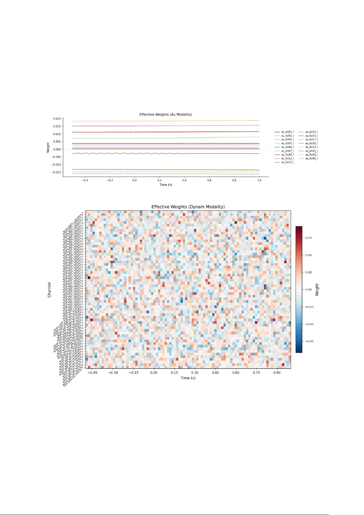
Ba y esian Inference of Psyc hometric V ariables F rom Brain and Beha vior in Implicit Asso ciation T ests Christian A. Kothe 1 Sean Mullen 1 Mic hael V. Bronstein 2,4 Gran t Hanada 1 Marcelo Cicconet 5 Aaron N. McInnes 2 Tim Mullen 1 Marc Aafjes 5 Scott R. Sp onheim 2,3 Alik S. Widge 2 1 In theon, La Jolla, CA, USA 2 Departmen t of Psyc hiatry and Beha vioral Sciences, Universit y of Minnesota, MN, USA 3 Minneap olis V A Medical Cen ter, MN, USA 4 Institute for Health Informatics, Univ ersit y of Minnesota, MN, USA 5 Delib erate AI, New Y ork, NY, USA { christian.kothe, sean.mullen } @intheon.io Abstract Obje ctive . W e establish a principled metho d for inferring men tal health related psyc hometric v ariables from neural and b ehavioral data using the Implicit Asso- ciation T est (IA T) as the data generation engine, aiming to ov ercome the limited predictiv e p erformance (typically under 0.7 area under the R OC curv e / AUC) of the gold-standard D-score metho d, which relies solely on reaction times. Appr o ach . W e prop ose a sparse hierarc hical Ba yesian mo del that leverages m ulti-mo dal data to predict exp eriences related to mental illness symptoms in new participan ts. The mo del is a m ultiv ariate generalization of the D-score with train- able parameters, engineered for parameter eﬃciency in the high-dimensional, small- cohort regime typical of IA T studies. Data from t wo IA T v ariants were analyzed, including a suicidalit y-related E-IA T ( n = 39) and a psychosis-related PSY-IA T ( n = 34). Main R esults . Our approac h ov ercomes a high inter-individual v ariability and lo w within-session eﬀect size in the dataset, reaching AUCs of 0.73 (E-IA T) and 0.76 (PSY-IA T) in the b est-p erforming mo dalit y conﬁgurations, though corrected 95% conﬁdence in terv als are wide (appro ximately ± 0 . 18) and results are marginally signiﬁcan t after false disco very rate (FDR) correction ( q = 0 . 10). Restricting the E-IA T to ma jor depressive disorder participan ts further impro ves A UC to 0.79 [0 . 62 , 0 . 97] (signiﬁcan t at q = 0 . 05). P erformance is on par with the b est tested reference metho ds (shrink age LDA and EEGNet) for each task, even though the latter w ere hand-adapted to these datasets, while the prop osed method was not. P oint-estimate accuracy was substan tially ab ov e near-chance D-scores (0.50–0.53 A UC) in b oth tasks, while maintaining more consistent p erformance across b oth tasks than any single reference metho d. Signiﬁc anc e . Our prop osed inference framework shows promise in enhancing IA T-based assessmen t of exp eriences related to en trapmen t and psychosis, and p o- ten tially other mental health conditions, although further v alidation on larger and indep enden t cohorts will b e needed to establish clinical utility . 1 1 In tro duction In men tal healthcare settings, diagnoses and treatmen ts b egin with inquiry ab out patien t exp eriences. Diagnostic lab els and treatment course therefore dep end on patien ts’ ability to accurately describ e their exp eriences. And yet, myriad factors undermine the ﬁdelit y of these descriptions. Because men tal illness is highly stigmatized, patien ts may fear that disclosure will usher in diﬀerential treatmen t from pro viders. They ma y also fear loss of autonomy if they disclose risk to themselv es or others. Ev en when patients w ant to tell pro viders their exp eriences, their descriptions can b e limited b y low levels of insigh t in to symptoms, particularly in conditions—lik e psyc hosis—that blur the lines of reality . Giv en these inﬂuences, it is not surprising that in terview-based to ols for the detection of men tal health conditions ha ve p o or sensitivities, ranging from no more than 41% (Suicide Ideation / SI) [ 1 ] to around 50% (Ma jor Depressive Disorder / MDD) [ 2 ] across many conditions. With this in mind, researc hers ha v e sought to dev elop alternativ e tools for mental health assessment that do not rely on self-rep orts. A signiﬁcant p ortion of these eﬀorts ha ve cen tered on Implicit Asso ciation T ests [ 3 ] (IA Ts), building on their widespread use in studies of so cial and cognitive psyc hology [ 4 ]. IA Ts serve to infer sub conscious asso ciations among tw o concepts (e.g. P epsi and Cok e) and tw o attributes (e.g. pleasan t and unpleasan t) [ 5 ]. In the traditional IA T, all four categories are mapp ed on to t w o resp onses, but the brief version of the task, known as the Brief-IA T (BIA T) [ 6 ] reduces the degree of coun ter-balancing and instructs sub jects to fo cus on just t wo category– resp onse mappings. This simpliﬁed task is b oth shorter (i.e., more feasible to administer in healthcare settings) and more accessible to clinical p opulations with potential cognitiv e deﬁcits. The trial-orien ted nature and binary classiﬁcation goal in the (B)IA T setup strongly suggest that this task ma y be amenable to a multiv ariate machine-learning (ML) based “deco ding” approach (e.g., [ 7 ]), where activity from sim ultaneously recorded brain and/or other signals suc h as EEG could be extracted relative to ev ents and serve as predictors used to infer the psyc hometric v ariable of interest. This machine-learning angle is at the heart of our approach, but, as will b e discussed, sev eral factors conspire to render the inference task considerably more complex and nuanced than the aforementioned conv en- tional ML setup. 1.1 Related W ork The consensus metho d for inference based on IA Ts is the D-score method (Diﬀerence score), whic h amoun ts to subtracting the a v erage resp onse latency in one of the paired concept/attribute blo c ks (of trials) from the a verage resp onse latency in the other paired concept/attribute blo cks, and dividing this diﬀerence b y the standard deviation of re- sp onse latency across all trials. As a result, the magnitude of D-scores is understo o d as an eﬀect size and the sign enco des its directionalit y (asso ciation betw een a certain pairing of concepts/attributes of interest presen t vs. absen t). The primary source from whic h this metho d dra ws its eﬀectiveness is the careful bal- ancing of t wo task conditions, which relies on matched stim uli, blo c k in terleaving, and prepro cessing of the reaction-time v ariable. Although this recip e has b een suﬃcient to ﬁnd relations b et ween implicit cognition and numerous outcomes (e.g., [ 8 ], [ 9 ]), it do es not fully mitigate sev eral imp ortan t shortcomings. D-scores op erate on a single IA T read- 2 out (reaction time), leaving the metho d fundamentally limited in its explanatory p ow er and prone to numerous confounds aﬀecting reaction times. D-scores are not naturally form ulated to work with other t yp es of features (e.g., brain activity), nor do es the ap- proac h readily suggest a metho d for learning feature w eigh tings from data. F or these and other reasons, the accuracy of mo dels classifying p eople based on IA T D-scores remains lo w (dep ending on the type of IA T, cohort, data quality , and ground-truthing strategy). As a notable example, D-scores w ere found to yield AUCs of 0.59–0.67 when predicting suicide attempts in p ediatric ER patients [ 10 ]. This is not suﬃcient for clinical utilit y . The shortcomings of traditional D-scores likely also contribute to their inability to explain practically signiﬁcan t amounts of v ariation in suicidality after accoun ting for explicit at- titudes [ 11 ], rendering it unclear whether IA T administration is worth while under this analytic regime. While looking b eyond reaction times migh t enable more information to b e extracted from IA Ts, surprisingly few studies hav e applied mac hine learning to m ulti-mo dal IA T data with the goal of predicting the primary quan tit y of in terest, that is, implicit biases. One study by Nikseresh t et al.[ 12 ] aimed to predict the participant’s implicit bias as measured b y the Race IA T, using 91 handcrafted features deriv ed from physiological sig- nals collected with the Empatica E4 wristband, including electrodermal activit y (ED A), Photopleth ysmography (PPG), heart rate and 3-axis accelerometer data, and using an X GBo ost [ 13 ] ML approach; this study ac hieved an accuracy of 76.1% in classifying par- ticipan ts as biased or un biased. Ho w ever, due to the highly Empatica E4 tailored feature extraction and absen t detail on ho w the XGBoost metho d was conﬁgured, this approach w as not readily adaptable to our data mo dalities and could not b e used as a comparison baseline. A study b y [ 14 ] employ ed facial action units (F AUs) in the context of an IA T task, although their goal diﬀered from ours in that they attempted to decide whether the participan t was “faking” their IA T results or not. They compared a num b er of ML metho ds including Naive Bay es, SVM, and Random F orests, and ac hiev ed accuracies in the 70–80% range; how ever, their metho d is not directly transferable to our setting since deco ding of the primary IA T v ariable requires structural matc hing to the task design (deco ding one v ariable from a con trast b etw een tw o others), as will b e discussed b elow. Bey ond these t wo studies, we w ere able to ﬁnd v arious uses of m ultiv ariate pattern analysis on IA T tasks for diverse exploratory purposes (for example [ 15 ], who analyzed systematic diﬀerences in gaze patterns using recurrence quan tiﬁcation analysis), but none of these w ere used in an out-of-sample prediction capacity or attempted to infer the primary task v ariable. Th us, for the purp ose of comparison w e primarily draw on mac hine learning metho ds that hav e pro ven adaptable to a wide range of trial-oriented cognitive tasks and hav e a trac k record of go o d p erformance on the mo dalities that w e collected, i.e., EEG, eye trac king, and to a lesser extent facial action units, and w e adapt these to our IA T scenario; this is describ ed in more detail in section 2.12 . 1.2 The Presen t Study Giv en the promise of m ulti-mo dal ML approaches and the inherent limitations of D-scores, w e prop ose a principled and adaptable metho d for inference of binary psyc hometric v ari- ables from IA T data, where it is assumed that auxiliary neural, bio and/or b ehavioral data (suc h as EEG, ey e tracking, or others) are collected while the participant is p erforming 3 the task. Our metho d retains the same assumption that underlies D-scores—that diﬀer- ences in resp onses to trials across IA T blo ck types are informativ e, instantiated within a mo dern ML framew ork and made parameter eﬃcient using structured sparsit y . The presen t study examines the p erformance of the prop osed method across t wo use- cases—inference ab out men tal health diagnoses and inference ab out the presence/absence of a type of clinically meaningful exp eriences, comparing it to the p erformance of b oth existing ML approaches and the traditional D-score method. W e sho w that our metho d is highly comp etitive with alternativ es and o vercomes c hallenges including small-to-medium training sets and generalization to new participan ts. It therefore represen ts an early but encouraging step tow ards elev ating IA Ts from a research tool to a more informativ e assessmen t, by demonstrating that substan tially more signal can b e extracted from IA T sessions than the prev ailing D-score metho d captures. 2 Materials and Metho ds 2.1 T ask Selection Data from t w o IA Ts—the Psyc hosis IA T (PSY-IA T a.k.a. P-IA T) [ 16 ] and the no v el En trapment IA T (E-IA T)—were used in the presen t study . The PSY-IA T presen ts par- ticipan ts with words describing psychosis-relev an t exp eriences (e.g., “visions”) in order to prob e implicit asso ciations b et ween the self and psyc hosis. The E-IA T is a no vel task dev elop ed to examine implicit attitudes regarding en trapment, whic h is thought to b e a central driv er of depression and suicidalit y [ 17 , 18 ]. In the presen t study , the E-IA T serv es primarily to explore the generalit y of our method across a second, structurally iden tical but thematically distinct IA T, op erationalized against a diﬀerent t yp e of dep en- den t v ariable (self-rep ort deriv ed from ecological momen tary assessmen t (EMA) rather than clinical diagnosis). 2.2 T ask Design The structure of b oth tasks was iden tical (i.e., only the task conten t diﬀered) and w as based on the BIA T (cf. [ 6 ] for a go o d introduction). W e note ho w ever that our metho d is also applicable to full-length IA Ts b y ignoring the additional exp erimen tal conditions presen t there, but the metho d was not tested with a full-length IA T. Two mo diﬁcations to the BIA T’s structure were made for the presen t study: the concept-attribute lab els were displa yed in the top center of the screen and aligned v ertically (instead of the concept displa yed top-left and the attribute display ed top-righ t) as shown in ﬁgure 1 , to minimize left-righ t ey e saccades that migh t factor in to the physiological measures b eing analyzed. W e also lengthened the task b ey ond the original 6 blocks of 20 trials eac h, with the goal of pro viding our model with more data allo wing it to better repro duce the high-dimensional v ariables inv olv ed. F or the E-IA T, we collected 12 blo cks of 30 trials each, for a total of 360 trials. F or the PSY-IA T, we collected 12 blo cks of 28 trials, for a total of 336 trials. Another example of the BIA T template is the Death Brief Implicit Asso ciation T ask (D-BIA T) [ 19 ], whic h we also administered, in a similarly mo diﬁed fashion. F or full details on our mo diﬁed task design and the stim ulus con tent, please see App endix A . Before attempting to classify participan ts based on IA T results, we generally discard data from trials sho wing stim uli that b elonged in the “not-me” category (of which there w ere 5 unique stimuli, i.e., “they”, “them”, etc.). These stimuli are discarded b ecause 4 ( a ) ( b ) ( c ) Figure 1: ( a ) Blo c k/trial structure used for E-IA T and PSY-IA T task designs. A “con- gruen t” or “incongruent” blo c k represents a blo ck of trials where the concept-attribute pair (i.e., “trapped/me”) display ed is in agreemen t or conﬂict, resp ectiv ely , with the sub- ject type (patient / control). ( b , c ) Screenshots of PSY-IA T task showing a trial from the tw o blo ck types. ( b ) depicts an incongruen t trial for a p erson with sc hizophrenia (a congruen t trial for a p erson without sc hizophrenia). ( c ) depicts a congruent trial for a p erson with sc hizophrenia (incongruen t for a p erson without schizophrenia). 5 the correct resp onse w ould alwa ys b e “not asso ciated,” rendering these less informativ e. As a result, the num b er of trials, for each session, seen by the mo del, was 270 for the E-IA T and 252 for the PSY-IA T. 2.3 Ph ysical Setup and Sensor Suite Sensor data were collected while sub jects p erformed a giv en task (E-IA T or PSY-IA T) in a dedicated data collection ro om. EEG was captured using a BioSemi ActiveTw o system and using the vendor’s 128-electro de ABC la yout, do wnsampled from 2048 Hz to 512 Hz at acquisition time, while video w as recorded using a FLIR Blackﬂy S R GB camera (running at 60 Hz). Pupillometry and eye tracking data w ere collected using a T obii Pro Nano infrared eye trac ker mounted along the b ottom of the monitor, also at 60 Hz. Multi-mo dal data capture and time synchronization w as p erformed using the Lab Streaming Lay er [ 20 ]. The task w as presen ted on a desktop PC using In theon’s (La Jolla, CA) Exp eriment Recorder task presen tation softw are and NeuroPype 1 soft ware for signal data capture, running on Windows 11. Eac h task was collected as part of a larger task battery that included other tasks and questionnaires that were not ev aluated here (the order of the tasks was balanced b etw een sub jects). Camera data collection was implemented using soft ware dev elop ed and tailored to this study by Delib erate AI (New Y ork, NY). A sc hematic and photograph of the setup are sho wn in ﬁgure 2 . ( a ) ( b ) Figure 2: ( a ) A diagram of the data capture setup sho wing the p ositioning of the sensors relativ e to the sub ject. ( b ) A photograph of the data collection setup at the Univ ersity of Minnesota used for the E-IA T task data collection. The same setup was used for the collection of the PSY-IA T task at the Minneap olis V A Medical Cen ter. 1 https://neuropype.io 6 2.4 P opulations and Datasets This study w as p erformed in accordance with the Declaration of Helsinki. This adult h uman sub ject study w as appro ved b y Adv arra IRB; ethical review w as ceded to this b oard by the Universit y of Minnesota IRB. All participan ts provided written informed consen t to participate in this study . Data collection w as conducted as part of a larger m ulti-site study on suicide ideation led by the Univ ersity of Minnesota. The PSY-IA T and E-IA T w ere secondary tasks in this study . The PSY-IA T w as collected at the Minneapolis V A Medical Center, with the exp er- imen tal group consisting of adults with a curren t or past history of non-pharmacologically induced psyc hosis, and a control group dra wn from the general p opulation ages 18–65 with no diagnosis of a mental illness. The E-IA T was collected at the Universit y of Minnesota Departmen t of Psyc hiatry , with the exp erimental group consisting of adults receiving treatment for ma jor depres- siv e disorder (MDD), and a control group (CTL) dra wn from the general population ages 18–65 and self-rep ortedly without any diagnosis of a mental illness. MDD partici- pan ts in the E-IA T sample were recruited from local in terven tional psyc hiatry clinics, and w ere required to b e on waitlist to receive transcranial magnetic stim ulation or k etamine therap y . The larger study w as fo cused on suicide ideation with Active SI as the primary metric and recruitmen t w as not directly based on c haracteristics central to the E-IA T (such as lev els of p erceiv ed en trapmen t) since it was a secondary task. All participants w ere also required to own a smartphone compatible with the EMA application used to ascertain E-IA T ground truth, or willing to use a study loaner phone. Exclusion criteria were con traindications to EEG (e.g., visible scalp abrasions), pregnancy , recent psyc hiatric hospitalization, or active military or Department of Defense employmen t, due to sp onsor requiremen ts. The order of the tw o IA T tasks (PSY-IA T, D-BIA T in the V A cohort, or E-IA T, D-BIA T at UMN) w as balanced across sub jects in eac h group. The sample consisted of all eligible participants who w ere recruitable at eac h site during a ﬁxed funding p erio d (April 2023 to September 2025). No formal p ow er anal- ysis w as p erformed to determine sample size. A p ost-ho c sensitivit y analysis using the Nadeau & Bengio [ 21 ] corrected v ariance framew ork indicates that, at our sample sizes and observed fold-lev el v ariability , the minimum detectable eﬀect size (MDES) at 80% p o w er and α = 0 . 05 corresp onds to a true A UC of approximately 0.70 (E-IA T) and 0.72 (PSY-IA T) for the resp ectiv e b est-p erforming conﬁgurations. This is oﬀered as a c haracterization of the study’s detection limits, not as evidence of adequate p ow er (cf. [ 22 ]). Our observ ed p oint-estimate A UCs of 0.73 and 0.76 exceed these thresholds, but the corrected 95% conﬁdence interv als (e.g., [0.56, 0.91] for the main full-sample E-IA T conﬁguration) are wide, reﬂecting the mo dest sample sizes, and readers should in terpret rep orted AUC v alues with this uncertain ty in mind. Additional exclusion criteria for analysis were (1) incomplete session record across the relev an t data b eing analyzed (EEG, eye track er, video, ev ent mark ers, questionnaire resp onses) due to data collection issues, and (2) b eha vior indicating improp er p erformance of the task due to lac k of task understanding, failure to b e a wak e and alert during the task (p er exp erimenter notes), or abnormally high error rates during task p erformance. The PSY-IA T was p erformed b y 44 sub jects, of whom 7 were excluded due incomplete/missing video data. Another three were excluded due to task b eha vior. Of the 34 sub jects 7 analyzed, 17 were from the experimental (psychosis) group, and 17 from the control group. The E-IA T w as p erformed b y 43 sub jects, of which tw o w ere excluded due to incomplete data, and tw o were excluded due to task b ehavior. Of the 39 sub jects included in the analysis, 33 w ere from in the MDD group and 6 in the control group. Note that the sub ject p opulations for the tw o tasks were from tw o separate sites and w ere non-o verlapping. 2.5 Ground T ruthing (Dep endent V ariables) In the case of the PSY-IA T, the ground truth for sub ject lab els w as the clinically do cu- men ted presence or absence of a history of psychosis. This was also the criterion for the exp erimen tal and con trol group assignmen t and was used as the dep enden t v ariable for the classiﬁcation rep orted here. Ground truth for the E-IA T was generated from self-rep orts. These self-rep orts w ere collected through ecological momentary assessmen ts (EMAs), surv eys completed by par- ticipan ts via their smartphones as they go about their daily liv es. P articipants w ere ask ed to complete these surveys 3x/day for sev en days prior to IA T data collection. The EMA battery generally co vered constructs relev an t to suicide (e.g., psyc hological pain, hop e- lessness). The six items sp eciﬁcally related to entrapmen t (and defeat, whic h we consider the same construct) were adapted from a widely used self-rep ort scale [ 23 ] and were in- ternally consisten t (within-p ersons omega-total = .73, b etw een-p ersons omega-total = .97). Item ratings were summed together at each EMA timepoint, then a veraged across timep oin ts to obtain a total en trapmen t score for eac h participan t. The entrapmen t score distribution w as approximately uniform (excess kurtosis = − 1 . 24, KS test vs. uniform p = 0 . 50; Hartigan’s dip test for bimo dality p = 0 . 80; similar for the MDD-only subset: kurtosis = − 1 . 14, KS p = 0 . 80, dip p = 0 . 78), with near-zero skewness. This score w as binarized at the whole-sample median (1.87), splitting participan ts into “high” (ab ov e- median) and “low” (b elo w-median) lev els of en trapment so as to conform to the o verall binary detection framew ork inv estigated in this article. This binarized v ersion was used as our dep enden t v ariable. Splits were not done separately b y participant group b ecause participan ts were not recruited based on entrapmen t levels, but rather on characteristics suc h as mental health diagnosis histories. All control-group (CTL) sub jects in the E-IA T dataset fell in to the low-en trapment group and among the MDD sub jects, 12 (36%) w ere lo w-entrapmen t and 21 (64%) w ere high-en trapment. T o rule out that the ML mo del is partly acting on a CTL/MDD con trast instead of, or in addition to, the entrapmen t con trast (and is therefore confounded), we also include a side analysis of ML p erformance on the MDD group only; that analysis sho ws that our mo del p erforms considerably b et- ter on MDD-only than on the broader MDD+CTL p opulation, how ev er w e rep ort here primarily results for the full sample since that w as our pre-sp eciﬁed analysis and w ould also b e more reﬂective the (presumed heterogeneous) broader p opulation. 2.6 Design and T esting Philosophy The metho d describ ed in this article is, by its m ulti-mo dal nature, inherently complex and has a n umber of prepro cessing and mo deling parameters. W e refrain from the com- mon practice of adapting these parameters in a data-contingen t manner, perhaps so as to impro ve p erformance, or in making apparently reasonable c hoices after ha ving reviewed the collected dataset via statistical summaries or visually . Rather, given the relatively mo dest size of datasets in v olved here, w e judge it to b e virtually imp ossible to do so 8 without inheren tly ov erﬁtting the approach to the dataset at hand in myriad wa ys, as called out in [ 24 ]. Av oiding this required relying on a largely pre-sp eciﬁed mo del and applying this mo del essentially unchanged to new data. In line with this, the approac h describ ed here w as originally dev elop ed on a series of separate tasks and datasets, in- cluding v arian ts of a custom autobiographical recall task and the D-BIA T. In this article w e describe both the mo del and its application to t wo new tasks to whic h it had not previously b een applied, essen tially serving as a ﬁrst description and v alidation study of the model; a separate article discusses the application of the mo del describ ed herein to one of these prior tasks (the D-BIA T). The transfer to new datasets is more lik ely to succeed if the mo del is largely free of parameters that are sensitiv e to a particular dataset and w ould require retuning. T o mak e this p ossible w e made the following design choices in our approac h: • Relying primarily on extensiv ely “battle-”tested generic prepro cessing comp onents for the v arious mo dalities, av oiding dataset-sp eciﬁc prepro cessing, and using only default or otherwise con v en tional parameter c hoices for data preparation and pre- pro cessing. • Avoiding p oten tially task-speciﬁc c hoices in the mo del (e.g., data-informed feature extraction) entirely and using generic structural prior knowledge instead. • Relying primarily on statistical mo deling that automatically adapts to the com- plexit y of the data at hand, using hierarc hical Ba yesian tec hniques. • Cho osing only w eakly informative “default” conﬁgurations for any remaining com- p onen ts. • F or parameters that are susp ected to b e somewhat dataset sp eciﬁc w e repro duce m ultiple settings in the results side by side. When comparing with reference metho ds from the literature (see section 2.12 for an o verview and App endix B for full details), a challenge w as that there were no existing metho ds that were reasonably w ell adapted to our combination of IA T task and data mo dalities. W e addressed this b y using generic metho ds or metho ds previously tested on similar data, whic h left the question of how to set their parameters (for example feature extraction) in a wa y that do es not unfairly p enalize these metho ds. T o account for this, w e tailored their parameters somewhat to the tw o tasks at hand, in some cases presented m ultiple c hoices side b y side, and we show that the proposed metho d remains comp etitive with and/or outp erforms these reference metho ds ev en in a setting that is fav orable to the latter. 2.7 Prepro cessing T o prepare data for use with the predictive mo del, we separately preprocessed eac h recording in a mo dalit y-sp eciﬁc manner using a previously developed robust prepro cessing pip eline. F or EEG, we emplo yed the data cleaning pip eline describ ed in [ 25 ] as imple- men ted in the NeuroPyp e softw are (In theon, La Jolla, CA). In the follo wing w e brieﬂy recap the main EEG prepro cessing steps and their parameters; for additional details, see the asso ciated references or the op en-source implementation in the clean rawdata 2 plugin for EEGLAB [ 26 ]. 2 https://github.com/sccn/clean rawdata 9 First, w e assigned 3D sensor/channel lo cations in a head-relative co ordinate system according to BioSemi’s cap-sp eciﬁc co ordinates ﬁle; session-sp eciﬁc co ordinate measure- men ts w ere not used. W e then remo ved any non-EEG channels, resampled the time series to 128 Hz using a polyphase implemen tation ( resample poly function provided b y SciPy [ 27 ]), remov ed the DC oﬀset b y subtracting the p er-c hannel median, and then applied a zero-phase (forward-bac kward) FIR highpass ﬁlter with a transition bandwidth of 0.25–0.5 Hz and 120 dB stop-band suppression. W e subsequen tly rejected noisy c han- nels whose high-frequency (ab o v e 45 Hz) conten t (magnitude in robust z-scores relativ e to all channels in the recording) exceeded 4 st. dev. or whose correlation with a robust estimate of the c hannel was b elow 0.7. The robust estimation (RANSAC) w as p erformed as in [ 28 ] and used 200 pseudorandom subsets of 15% of c hannels eac h. W e then pro jected high-amplitude artifacts out of the data using the artifact subspace reconstruction (ASR) metho d [ 25 ] using a cutoﬀ of 15 st. dev., and subsequently rejected an y time windo ws that con tained residual high-amplitude artifacts if their p o wer in at least 25% of c hannels exceeded a − 4 to +7 st. dev. range (also using robust z-scores across all c hannels). Next w e suppressed line noise and other high-frequency con ten t using a zero-phase FIR lo wpass ﬁlter with 40–45 Hz transition band and 50 dB stopband suppression, and in terp olated an y previously rejected channels using spherical spline in terp olation [ 29 ]. Lastly , w e re- referenced all c hannels to the common av erage and retained a subset of 64 equidistant c hannels using a metho d analogous to that of the METH to olb o x 3 . A reduction from 128 to 64 c hannels had previously b een identiﬁed as a go o d tradeoﬀ of mo del degrees of freedom vs. spatial resolution in analyses of the D-BIA T and earlier autobiographical tasks and was retained for this study in line with our parameterization philosoph y . All other prepro cessing parameters matc h NeuroPyp e’s default pro cessing pip eline for ma- c hine learning, except for a more forgiving ASR cutoﬀ (default is 10) and a highpass ﬁlter b etter adapted to even t-related potentials. F rom the participan t videos, we extracted F acial Action Units (F AUs). F A U mea- suremen ts employ ed a prepro cessing pip eline by Delib erate AI (New Y ork, NY), which relies on MediaPip e [ 30 ], Op enF ace [ 31 ], and custom libraries to derive time-v arying F A U estimates according to the F acial Action Coding System (F A CS) [ 32 ] plus head orien- tation and gaze vectors, along with the discrete ﬁrst and second time deriv ativ es of all c hannels (i.e. “dynamic” features). The follo wing F ACS-deﬁned A Us were extracted by this pipeline: 1, 2, 4, 5, 6, 7, 9, 10, 12, 14, 15, 17, 20, 23, 25, 26, and 45. F or the eye track- ing mo dalit y w e use all channels deliv ered by the T obii ey e trac ker, including estimated screen co ordinates, pupil diameter, and pupil conﬁdence. W e also corrected (dela y ed) stim ulus even t time stamps according to a photo dio de-measured end-to-end on-screen stim ulus presentation dela y of 54 ms. W e use the following acron yms for these mo dalities in the remainder of the article: EEG (prepro cessed EEG), gaze (ey e trac ker), F AU (facial action unit estimates), and Dyn (v arious dynamic / time-deriv ative features). F ollowing contin uous-data preprocessing, stimulus-lock ed segmen ts w ere extracted from eac h mo dality for each trial. W e rejected segments where time windo ws that had previously been remo v ed due to artifacts fell within a range of − 0 . 5 to 1 . 0 seconds relativ e to stim ulus onset, and extracted the remaining segments spanning this same time range from F A U and gaze streams, resp ectiv ely . F or EEG, to reduce the degrees of freedom of the mo del, we retained shorter time segments spanning − 0 . 1 to 0 . 45 seconds; this time window was previously determined on the D-BIA T task. This yielded, for a given trial t , an EEG segmen t X EEG t ∈ R C EEG × K EEG where C EEG = 64 is the n umber of EEG 3 Guido Nolte’s MEG & EEG T o olb o x of Ham burg 10 c hannels and K EEG = 71 is the num b er of EEG time points, along with an F A U segmen t X F AU t ∈ R 41 × 96 , a Dyn segment X Dyn t ∈ R 41 × 96 , and a gaze segmen t X gaze t ∈ R 6 × 96 , of whic h not necessarily all mo dalities will b e used in a given mo del. T o k eep notation ligh t, w e omit the trial and mo dalit y sub/sup erscripts from symbols where clear from the con text. Before training our predictiv e mo dels, we ﬁrst standardized eac h (zero-mean) c hannel in eac h mo dality m to unit v ariance on the respective training set. In line with standard practice we treat the v ector of scales s m ∈ R C m as a learnable mo del parameter that is re-ﬁt on eac h training set and applied (but not recomputed) on the resp ective test set(s). T o prepare data for traditional neural analyses, sp eciﬁcally the ev ent-related p oten- tial (ERP) ﬁgures (section 3.4 ), the prepro cessing steps w ere largely similar to what is describ ed ab ov e with minor mo diﬁcations in line with more typical pro cessing chains used in ERP studies. W e set the FIR highpass ﬁlter with a transition bandwidth of 0.1–0.2 Hz, the FIR lowpass ﬁlter with a transition bandwidth of 15–20 Hz, and set ASR cutoﬀ threshold to 10 st. dev.. ERPs were furthermore baseline-corrected to 100 ms of pre-stim ulus activit y after segment extraction. F or group-lev el statistics, w e use mass univ ariate ANO V As on v arious factors (e.g. blo c k conditions, clinical status, etc.) for b oth within-sub jects and b et w een-sub jects conditions. 2.8 Predictiv e Mo del 2.8.1 Goal Our mo del is designed to accept a recording (“session”) w orth of (appropriately seg- men ted) brain and/or b ehavioral time-series data collected from a person across one or more measuremen t mo dalities while p erforming the IA T. It then predicts from these measures the probability that the p erson displays a p ositiv e implicit association with the psychometric v ariable b eing tested. This also yields (through subtraction from 1) the probabilit y of the negativ e even t, that is, the p erson not displa ying a p ositiv e asso ciation. F or simplicity , we equate sessions with participants in the following, i.e., one participant yields one session, as this is the structure of b oth our datasets. 2.8.2 Ov erall F ramework Our approach will b e to design a type of hierarchical generalized linear mo del (GLM), optionally m ulti-mo dal, that explains the dep enden t v ariable y (1 if p ositive or 0 other- wise) as a function of the given p er-session observ ations, along with mo del parameters that w e will learn from a given training sample. The mo del therefore has to generalize from the training cohort of participan ts to a new participant; this is made challenging due to the relatively mo dest n um b er of participants in t ypical IA T study datasets, in- cluding the ones analyzed here (with n = 39 for the E-IA T and 34 for the PSY-IA T). The relativ ely large num b er of explanatory v ariables in the mo dalities of interest (EEG, F AU) across the p oten tially relev ant time p oints and channels leads to many degrees of free- dom d f in the mo del (10,000s if not carefully controlled). While this could b e reduced with detailed task- and mo dality-speciﬁc feature engineering (e.g., enco ding presumed relev ant c hannels and/or time slices), the necessary knowledge is often not a v ailable in a new and/or relatively under-studied mac hine-learning task suc h as the one studied here, and w ould hav e to b e inferred from the data at hand alongside the rest of mo del. As 11 noted, w e refrain from this here and w e instead employ a (hierarc hical) Bay esian ap- proac h, which allows us to impose strong structural priors to con trol mo del complexit y without requiring task-sp eciﬁc kno wledge. A k ey feature of our mo del is that we rely on a sparse Ba yesian learning (SBL) strategy , which ac hiev es high parameter eﬃciency and th us low eﬀectiv e mo del complexit y , while comparing fa vorably to the con vex l 1 p enalt y (a.k.a. the LASSO) p opular in mac hine learning due to the latter suﬀering more from o ver-shrinking of non-zero mo del coeﬃcients [ 33 ]. A second key strategy is to ﬁt the mo del at the (p o oled) single-trial level , thus lev er- aging single-trial v ariabilit y as a stand-in for participan t-lev el v ariabilit y that w e ha v e not observed (for lac k of a larger dataset). W e will discuss these tradeoﬀs in the next section. In the follo wing we ﬁrst presen t the prediction rule in frequen tist terms and then la y out the Ba yesian mo del used to infer the v arious parameters. 2.8.3 Prediction Rule W e aim to estimate P ( y = 1 | X , θ ) where X are the observ ed/indep endent v ariables (measuremen ts), y is the dep endent v ariable, and θ is the collection of mo del parameters. While the mo del can in principle accommo date a v ariety of forms for y (e.g., binary , con tinuous, or ordinal) using appropriate lik eliho o d functions, w e restrict ourselves here to the elementary binary (detection) case, which is w ell matc hed to the detection task at hand. W e mo del the session-level success probabilit y as P ( y = 1 | X , θ ) = logistic( z ) where z ∈ R is the session-lev el logit and is ultimately a weigh ted linear com bination of appropriately segmented observ ations from the session of interest, which mak es our mo del a t yp e of logistic regression. The output of the model is in terpretable as a detection probabilit y that may b e thresholded by the practitioner according to a decision threshold that ac hieves, for example, a suitable sensitivity/speciﬁcity tradeoﬀ. In our setup and for ev aluation purp oses, we set the decision threshold at the canonical P ( y = 1) = 0 . 5. The mo del has to in tegrate evidence (i.e., logits) across eac h individual trial t ∈ { 1 , . . . , T } of the exp erimen tal session to yield z . W e employ the form ula z = ω T P T t =1 z t ; that is, z is an av erage of the p er-trial evidence scores z t w eighted b y a scale factor ω ∈ R . ω can b e in terpreted as a ratio of session-lev el evidence (logit magnitude) to single-trial lev el evidence and is the sole parameter of the mo del that is ﬁt at the session level, as part of a tw o-stage ﬁtting pro cedure (see section 2.10 for more detail). T o streamline notation w e treat all data mo dalities to ha ve generally matrix-v ariate p er-trial observ ations, so for an y given mo dalit y m and trial t w e observ e a matrix X m t . F or a single mo dalit y (for example, EEG only), w e th us ha ve z t = ⟨ X m t , W m t ⟩ F , i.e., a linear function of the data, where we denote b y ⟨ A , B ⟩ F := trace( A ⊤ B ) the F rob enius inner product of tw o matrices, and where W m t is the learnable w eigh t matrix for modality m . In the multi-modal case we treat z t as a w eigh ted sum across mo dalities, using a separate p er-mo dalit y w eighting α m . Th us, in the general case of M mo dalities w e ha ve: z t = M X m =1 α m ⟨ X m t , W m t ⟩ F . (1) W e write the w eigh t matrices as (technically) trial-dep enden t, and this is a crucial feature of our mo del that has its ro ots in the standard D-score metho d for analyzing IA T tasks: in D-scoring, D (the analog to our z ) is the (scaled) mean of all reaction times (observ ations) in the incongruent condition min us the scaled mean of reaction times for 12 the congruent condition, as in D = M incongruent − M congruent S D po oled . W e can capture this in our model by making our w eigh ts formally condition-sp eciﬁc, such that, for eac h in congruen t trial t ∈ I w e ﬁx W m t to a single learnable matrix W m I and lik ewise for eac h c on gruent trial t ∈ C w e ﬁx W m t = W m C . The diﬀerence structure in the ab ov e form ula then suggests a simple “mirror” constraint W m I = − W m C on the w eights. Clearly there exists also a v ariant that do es not imp ose a sign rev ersal, but this results in a mo del that is not a congruency detector but whic h instead aims to directly deco de the participan t lab el, regardless of the blo ck condition. W e brieﬂy touc h on this in the con text of the reference metho ds (App endix B ). Another v ariant w ould allo w the tw o weigh t matrices to b e fully indep endent —how ev er, analysis of IA T tasks is extremely sensitive to the balance of the tw o (symmetric b y design) conditions, which lik ely requires statistical constrain ts on suc h a pair of matrices, for example on the norm of the diﬀerences; the design space for this is large and we do not explore these options in this article. F or the aforemen tioned balancing reason, our mo del also includes no in tercept parameter, although such a parameter may b e included if additional auxiliary predictors (e.g., questionnaire resp onses, etc.) w ere added to the mo del. Bey ond the basic prediction rule outlined ab o ve, when the learned p osterior distri- bution o ver relev an t parameters θ is used in the form ula, this giv es rise to the p osterior predictiv e distribution for P ( y = 1 | X , θ ). 2.9 Learning W e p ose learning of the relev ant mo del parameters as a Ba y esian inference problem where w e mo del the binary outcome v ariable y using a Bernoulli likelihoo d giv en the logits z , i.e., y ∼ Bernoulli(logistic( z )) . (2) When deﬁning prior distributions for the remaining parameters, our strategy will b e to enco de primarily structur al kno wledge into the priors. F undamen tally , the type of prior for a w eigh t matrix W m (or by symmetry , its mirror-constrained v arian t) depends on the nature of the mo dality and how w e exp ect the eﬀect of in terest to manifest in the w eights. Due to the mirror constraint, our weigh t matrix b ehav es eﬀectiv ely as a trial-level (in)congruency detector and, when viewed as a type of (generalized) linear mo del, these w eights ma y b e understo o d to a ﬁrst appro ximation as mo deling a “con trast” b et ween observ ations of congruen t vs. incongruen t IA T trials, resp ectively . In practice, this b eing a decoding mo del, the weigh ts will furthermore inv olv e correction terms that p erform suppression and p oten tially cancellation of n uisance in terference or noise. The simplest type of prior w e may consider is the standard normal, W m ∼ N (0 , 1), whic h may be appropriate for mo dalities with v ery few predictors (e.g., the scalar p er- trial (log-)reaction time). How ev er, already for the 6-c hannel gaze modality , w e ha ve, at 60 Hz sampling rate, w ell o ver 500 degrees of freedom in the mo del—lik ely to o large to allow for reliable ﬁtting from ev en a 50-participant dataset. W e oﬀer a bac k-of-the- en velope attempt to quantify this in App endix C . Consequen tly , for this and the more complex time-series observ ations, a stronger prior is v ery lik ely needed. W e hav e found the following assumptions to b e suﬃcien t for a range of typical b ehavioral time-series mo dalities: optionally smo othness (slow changes) in weigh ts along the time dimension of 13 the w eigh t matrix, and group-wise sparsit y along the channels dimension of the matrix. Sp eciﬁcally , we mo del W gaze and W F AU as b oth group-sparse and smo oth, and W Dyn as group-sparse (but not necessarily smo oth). W e formalize these assumptions using a group ed horsesho e prior [ 34 ] for the Dyn mo dality , and a group ed horsesho e where the unscaled weigh t matrix is dra wn from a Gaussian random walk (GR W) pro cess with non-zero initial in tercept for the gaze and F AU mo dalities. F ormally , w e ha ve τ m ∼ HalfCauc hy(1 . 0) , τ m ∈ R + (3) λ m ∼ HalfCauc hy(1 . 0) , λ m ∈ R C m + (4) β Dyn ∼ Normal(0 . 0 , 1 . 0) , β Dyn ∈ R C Dyn × K Dyn (5) β gaze ∼ GR W( σ 0 , σ gaze i ) , β gaze ∈ R C gaze × K gaze (6) β F AU ∼ GR W( σ 0 , σ F AU i ) , β F AU ∈ R C F AU × K F AU (7) where GR W is the Gaussian random walk prior with initial in tercept scale σ 0 = 1 . 0 and learnable innov ation scale σ m i . F ollowing the group ed horsesho e construction, the resulting sparse w eight matrix is then W m = τ m diag( λ m ) β m , i.e., a pro duct of a global scale factor τ m , a diagonal matrix of p er-channel scales diag ( λ m ), and the unscaled weigh t matrix β m . F or EEG, the situation is complicated considerably by the fact that relev an t EEG activit y is t ypically not conﬁned to a small set of channels o wing to electrical volume conduction, and thus W EEG is generally not group-sparse in c hannels. Ho wev er, w e may instead assume that only a few latent brain sour c es diﬀer in their activit y across the con trast of in terest (congruen t vs incongruen t) so that the weigh t matrix is eﬀectively group-sparse in terms of brain sources. W e c ho ose here a formulation of this that is to our kno wledge no v el, and whic h w orks as follows; this construction constitutes a core part of our metho d for the EEG case. W e mo del the scalp forw ard pro jection of the relev ant brain activit y contrast as a latent matrix A ∈ R C × K whose prior will be chosen to encode the laten t source-lev el sparsit y and smo othness, whic h we choose to b e a matrix-normal distribution as in A ∼ MatrixNormal( 0 , Σ U , Σ V ) (8) and which is parameterized b y a row (spatial) cov ariance matrix Σ U ∈ R C × C and column (temp oral) co v ariance matrix Σ V ∈ R K × K . The latter w e c ho ose as the co v ariance matrix of a GR W pro cess, whic h is deﬁned as Σ V = σ 2 0 11 ⊤ + σ 2 i J J ⊤ where 1 is the vector of all ones of length K and J is the K × K unit low er-triangular matrix of ones. The spatial co v ariance matrix Σ U is mo deled as the sum of the scalp forward pro jections of p er-source co v ariance matrices Γ s ∈ R 3 × 3 and a bac kground term Σ ϵ ∈ R C × C , and is therefore: Σ U = Σ ϵ + S X s =1 L s Γ s L ⊤ s . (9) where L ∈ R C × 3 S is an EEG lead-ﬁeld matrix with ﬂexible (3-axis) orien tations and L s is the triplet of columns corresp onding to source s . The spatial comp onent is essen tially the same prior emplo yed b y the Champagne M/EEG source estimation mo del [ 35 ] while the o verall spatio-temp oral construction for A is an instance of the Dugh framework [ 36 ] (a spatio-temp oral generalization of Cham- pagne with learnable temp oral dynamics), here using the GR W pro cess for the temp oral co v ariance. 14 W e then connect the latent contrast matrix A to the deco ding w eight matrix W EEG via the Haufe transform [ 37 ] (eq. 6) A = Σ X W κ , which w e rearrange and simplify to yield W EEG = Σ − 1 X A . The resulting weigh t matrix can then be viewed as a t yp e of spatial ﬁlter that is designed to pick up the con trast enco ded in A while suppressing noise and in terference captured in the empirical data co v ariance matrix Σ X . This model is also closely connected to linear discriminan t analysis (LDA), where A pla ys the role of a diﬀerence in p er-condition means (the contrast) and Σ X is the co v ariance matrix. The latter diﬀers from the av erage class-conditional cov ariance matrix Σ ¯ c used in LDA in that the cov ariance of A contributes to Σ X but not Σ ¯ c , but the eﬀect only impacts the output scale and is absorb ed in to the scale term κ in the Haufe transform (as discussed in [ 37 ]). This parameter can b e made learnable in the Bay esian model, but in our testing this made little to no diﬀerence in practice since the scale can also b e learned as part of A itself, and is therefore omitted from the ab o ve form ulation. The main no v el asp ect is the transformation of what is typically taken as a sparse source imaging model in to a sparse discriminant mo del with the help of the data co v ari- ance matrix Σ X . The lead-ﬁeld matrix L in the ab o v e formulation w as derived from the ICBM 152- participan t av erage T1-weigh ted scan [ 38 ] from whic h we reconstructed a 4-shell brain mo del using F reesurfer [ 39 ]. This w as then co-registered with the 68-region Desik an- Killian y atlas [ 40 ] and the 64 channel BioSemi montage using BrainStorm [ 41 ] and was used to estimate an initial 5003-vertex ﬂexible-orien tation lead-ﬁeld matrix. The lead- ﬁeld matrix L as used in the model w as then preprocessed by normalizing eac h row to unit norm and kernel-smoothing as done in the Smo oth Champagne v arian t [ 42 ] (here applied to vertices rather than v oxels), using a kernel width set to m = 2 times a verage distance b et w een adjacent v ertices [ 42 ] (default is 2 v oxels). Also as in Smo oth Champagne, the Γ s h yp er-parameters w ere tied across source v ertices in the same atlas region and parameterized to ha v e spherical co v ariance, that is, Γ s = γ 2 r I 3 where I 3 is the 3 × 3 iden tity matrix and γ 2 r is the scalar v ariance of the region r into whic h v ertex s falls. As in most Champagne v arian ts, the v ector γ of h yp er-parameters w as estimated using empirical Ba yes, although here estimation w as done as part of the sto chastic v aria- tional inference (SVI) for the ov erall mo del, instead of the iterativ e closed-form up dates prev alent in prior literature, ultimately because our multi-modal deco ding mo del is con- siderably more complex than these source imaging tec hniques. As discussed in [ 43 ], the sparse Ba yesian learning formulation underlying Champagne can b e instantiated using a v ariety of hyper-priors for the γ r parameters, and ﬂat hyper-priors tend to b e preferred since they simplify closed-form up dates. Since we are under no such constrain ts in the SVI framew ork, we use in our mo del a w eakly informative (half-) student-T hyper-prior with ν = 3 degrees of freedom and scale 0 . 1 4 : γ r ∼ HalfStuden tT( ν , 0 . 1) , γ r ∈ R + (10) W e mo del the p er-mo dalit y weigh ts α m and GR W innov ation scale σ m i as follows: α m ∼ Normal(0 . 0 , 1 . 0) , α m ∈ R (11) σ m i ∼ HalfNormal(0 . 1) , σ m i ∈ R + (12) 4 Wipf and Nagara jan [ 43 ] argue that the prior c hoice is relativ ely inconsequen tial, and we ﬁnd this to o, in that the prior t yp e (e.g., ﬂat vs. StudentT) and scale had almost no eﬀect on deco ding p erformance in prior exploration on D-BIA T data; how ever, the sparsity and th us interpretabilit y of the weigh t map w as aﬀected, and th us w e used non-ﬂat priors in this work. 15 Our prior analysis of the D-BIA T task had suggested an even tigh ter h yp er-prior with a scale of 0.01 for σ m i , but this seemed unreasonably rigid for a generic method and w as th us relaxed to 0.1 as in the ab o ve formulation. W e ho w ev er include a side-b y-side analysis of the tw o parameter c hoices. The EEG data cov ariance matrix w as estimated as Σ X = (1 − λ ) Σ post + λ diag ( Σ post ) where Σ post is the empirical sample co v ariance matrix of the p o oled p ost-stimulus EEG activit y across the training data and λ = 0 . 01 is a shrink age regularization parameter, mainly to prev ent degeneracy . The noise cov ariance matrix Σ ϵ w as in turn estimated from the empirical pre-stimulus cov ariance matrix Σ pre using VBF A based on [ 44 ] (here using 5 in terference factors) according to standard Champagne M/EEG practice. Note VBF A is implicitly regularized and therefore Σ ϵ do es not require a λ term. An ov erview of the complete mo del is shown in ﬁgure 3 . Since the Dugh-t yp e EEG prior is relatively complex and one ma y w onder if a simpler alternativ e would b e comp etitive, w e also ev aluated an alternative form ulation that relies on a somewhat more conv en tional lo w-rank mo deling assumption, where it is assumed that the w eight matrix W EEG is low-rank (using a horsesho e prior applied to its singular v alues), while its right singular vectors follo w the same GR W prior as in the other form u- lations (imp osing temp oral smo othness); this mo del p erformed less w ell in our ev aluation and is only noted here for completeness. W e refer to the o verall mo del throughout the remainder of the article as uniﬁed sparse Ba yesian learning for IA Ts (USBL-IA T or short USBL) in that it represents a multi-modal instan tiation of SBL that draws on a ﬂexible modality-speciﬁc rep ertoire of sparse priors. Inference w as p erformed in NeuroPyp e using the numpyro [ 45 ] probabilistic program- ming language using its stochastic v ariational inference [ 46 ] approac h in conjunction with the graph-based v ariational ob jectiv e [ 47 ], and using a Laplace p osterior approximation. F or optimization w e used the Optax [ 48 ] implemen tation of Adam [ 49 ] with gradient norm clipping at 1.0 and using a learning rate of 0.01 that was exp onen tially decay ed o ver 5000 steps to a ﬁnal v alue of 0.0025. This conv erges in ab out 3-5 minutes on an R TX3080-class NVIDIA GPU dep ending on the com bination of mo dalities included in the mo del. W e did not encoun ter evidence of lo cal-minima issues with the optimization problem, in that runs from diﬀeren t pseudo-random initializations tended to con verge to similar or iden tical ﬁnal p erformance. A full cross-v alidated ev aluation run with/without conﬁdence calibration takes ca. 2.5h/12h on a single GPU p er conﬁguration, although note that routine re-ﬁtting of the model on a growing data corpus may not require a full cross-v alidation and re-ev aluation, and a m ulti-GPU system reduces this b y the num b er of GPUs. 2.10 Conﬁdence Calibration Conﬁdence calibration infers the scale factor ω for the mo del’s logits z . The primary reason wh y this parameter cannot be readily estimated in one step along with the re- mainder of the mo del is that our primary observ ations are at the single-trial level, where the participant-lev el z is merely a derived v ariable, resulting in model conﬁdence b e- ing calibrated to the evidence av ailable in a single trial, while total evidence across a session w orth of trials will typically b e larger. F urthermore, if w e included an addi- tional participant-lev el observ ation and likelihoo d term in the mo del to calibrate ω , this w ould risk considerable ov erﬁtting of the o verall mo del at mo dest num b ers of training participan ts (also empirically observ ed in prior analysis on B-DIA T data), since the p er- 16 Figure 3: Diagram for the USBL mo del, sho wn for a com bination of EEG and F AU mo dalities. Here T is the num b er of trials in a session and P is the num b er of participan ts in the dataset being analyzed. The mo dality superscripts EEG and F A U ha ve b een shortened to E and F, resp ectiv ely . X E and X F are the preprocessed observ ations for the curren t trial and participant (subscripts omitted) and W E and W F are the asso ciated w eight matrices. y is the dep endent v ariable for the curren t participan t (same for all trials), α is the vector of p er-mo dalit y w eigh ts α m , A is the latent EEG con trast matrix, β F is the unscaled w eight matrix for the F A U mo dality and τ and λ are the global and lo cal (p er-channel) horsesho e scales, resp ectiv ely . Σ U is the mo del-deriv ed EEG spatial co v ariance matrix and σ i is the learned innov ation scale for the EEG smo othing (GR W) prior. γ is the vector of p er-region h yp er-parameters estimated as part of the mo del. 17 participan t observ ation would also inﬂuence the high-dimensional weigh t matrices, among others. Instead, we ﬁt the mo del using a tw o-stage pro cedure: ﬁrst the inner mo del is ﬁt (as describ ed in section 2.9 , ﬁxing ω = 1), and then ω is inferred. F or the latter w e use a strategy similar to Platt scaling [ 50 ] where we form a posterior predictive distribution p ( z p ) ov er the resp ectiv e session-lev el prediction z p that we ev aluate separately for one or more held-out participan ts p as part of an internal cross-v alidation. As motiv ated in [ 50 ], suc h a pro cedure will absorb the generalization error of the metho d in to its conﬁdence. Giv en the distribution o ver z p , we mo del ω ∼ HalfCauc hy(10 . 0) , ω ∈ R + (13) y p ∼ Bernoulli(logistic( ω z p )) (14) where we pulled ω out of the formula for z p . This uses a relatively lo ose prior for ω that allows the conﬁdence to b e increased considerably if supp orted b y the data. Here, y p is the lab el of each resp ective held-out test-set participan t. If a full p osterior for ω is inferred, the resulting comp osite mo del is then also fully Bay esian. W e ﬁt this p ortion of the mo del also using numpyro , using Marko v-Chain Mon te Carlo (MCMC) [ 51 ] and sp eciﬁcally the No U-T urn Sampler (NUTS) [ 52 ] using 500 w armup samples and 1000 retained samples. T o av oid p otential confusion, w e note that, when the resulting comp osite model- ﬁtting itself is being ev aluated in an o verall cross-v alidation (as will be discussed in the following), the latter constitutes an outer cross-v alidation while the aforementioned Platt scaling-“internal” cross-v alidation plays the role of a neste d cross-v alidation that is rigorously conﬁned to eac h resp ective (outer) training set (e.g., [ 53 ]); as this step can m ultiply the o verall compute exp ense sev eral-fold; for the nested level w e use a 5-fold stratiﬁed cross-v alidation (holding out participants). 2.11 Ev aluation T o assess the p erformance of our model when generalizing to new participan ts, w e em- plo yed a 10x repeated 5-fold randomized and stratiﬁed (outer) cross-v alidation, holding out whole participan ts 5 , in line with curren t b est practices (e.g., [ 54 ], who recommend a similar conﬁguration). W e then quantiﬁed, on each test set, the A UC as our primary metric along with sensitivit y and sp eciﬁcity on the p o oled test-set predictions. Notably , when using a decision threshold at P = 0 . 5 (or equiv alen tly , z = 0), the classiﬁcation decision is in v ariant under conﬁdence rescaling via ω and thus metrics such as accuracy , sensitivit y , or sp eciﬁcity remain unaﬀected. The A UC, being sensitive only to ranks, also remains unaﬀected. F or these reasons and for computational expediency , this step w as not applied for the main result tables (tables 1 , 2 ) and w e assumed ω = 1, but full conﬁdence rescaling was applied to generate results in table 3 . W e tested the AUC of the prop osed metho d for signiﬁcant diﬀerence from a chance lev el of 0.5 using a cor- rected resampled t-test, whic h accoun ts for the rep eated nature of the cross-v alidation [ 21 ]. These p-v alues w ere further corrected using the Benjamini-Ho ch b erg false discov ery rate pro cedure [ 55 ] across all 16 instantiations of the prop osed metho d across mo dalities, tasks, and an additional application to MDD-only participan ts, but not co vering mo di- ﬁed v ariants included to supp ort side remarks in the paper or to illustrate sensitivity to 5 This amounts to 7–10 participants p er fold dep ending on task (E-IA T or PSY-IA T) and fold-to-fold v ariation due to rounding. 18 h yp er-parameters. In addition to fold-lev el standard deviations, we rep ort corrected 95% conﬁdence in terv als on the mean p erformance metrics (tables 1 , 2 ), computed using the Nadeau & Bengio v ariance correction ˆ σ 2 corr = (1 / ( k r ) + n 2 /n 1 ) ˆ σ 2 where k = 5, r = 10, and n 1 , n 2 are the training and test set sizes p er fold, resp ectiv ely . This correction accoun ts for the non-indep endence of o verlapping training sets across folds 6 . 2.12 Reference Metho ds Due to the few applicable reference methods to compare with, w e c hose comparison baselines as follo ws. F or EEG, w e employ ed a strong linear method (sLDA on linear features, as describ ed in [ 7 ]) that is known to work w ell on tasks that exhibit salien t even t- related p oten tial (ERP) eﬀects (section Neural Con trast Maps conﬁrms that this is the case here). Additionally w e compare with a gold-standard deep learning metho d (EEGNet [ 56 ]) that is understoo d to b e suitable for b oth ERPs and oscillatory pro cesses. W e reasoned that ey e-tracking and AU time courses exhibit qualitatively similar time courses as EEG even t-related potentials (but pla ying out o ver longer time scales), and therefore w e use these same metho ds also for pairings of EEG and non-EEG mo dalities (suitably extended and using accordingly longer time windo ws, see App endix B for details), and w e use these metho ds also for the case where EEG is not included. T o shed more light on the eﬀectiveness of the sparse Bay esian priors and the Bay esian pro cedure in particular (as opp osed to regularization and empirical risk minimization), while using the same underlying features, w e also compare with a robust (scikit-learn) implemen tation of l 2 -regularized logistic regression (sho wn as L2LR in the results tables). W e test this approac h on all mo dality combinations, EEG or otherwise. All methods share the same prepro cessing chain as the prop osed method. Notably , all implemen ted reference methods follo w the congruency detection strategy of the Ba yesian model (realized by the mirror constrain t in the latter and b y a lab el “reco ding” construction describ ed in App endix B ). One may wonder whether dir e ct de- co ding of the participant’s lab el regardless of block t yp e w ould b e possible. In prior work w e ha ve generally found, b oth in the Bay esian mo del and in the reference metho ds, that this do es not app ear to b e the case and p erformance across all metho ds in this scenario w as considerably w eak er, often at or near chance level. W e consider a full exploration of this route out of scop e for this article but include a setup in the comparison matrix to demonstrate this, where we use the single b est-p erforming linear model (PSY-IA T, sLD A, EEG-only) and w e adjust the model to directly deco de the participan t label (th us skipping the construction discussed in App endix B ); this approac h is iden tiﬁed as “sLD A (direct)”. 3 Results In the follo wing section, w e review results across a bank of comparisons, separately for eac h of the tw o tasks. W e generally sho w results for all combinations of mo dalities except where noted (e.g., to sav e table space where a mo dality w as universally uninformative). F or ea c h table cell we reproduce the mean and standard deviation of the resp ective 6 F or our sp eciﬁc design parameters, the corrected CI half-width yields CIs that are numerically close to mean SD. This is a coincidence of these particular parameters and do es not hold in general. 19 p erformance metric across the 10 × 5 cross-v alidation folds, corresp onding to 50 train/test splits. 3.1 Deco ding P erformance 3.1.1 E-IA T W e tested the proposed mo del across a range of mo dalit y subsets to ascertain the individ- ual utilit y of eac h modality alone and in combination with others. Results are reproduced in table 1 below. Additionally , we compared the metho d with a set of reference metho ds from prior literature (b ottom of table). T able 1: Performance comparison b et w een the prop osed metho d and a battery of refer- ence metho ds across diﬀerent mo dalit y com binations, on E-IA T data. Alternative h yp er- prior settings are rep orted in table 4 . Note results on F AU and Dyn features in the E-IA T w ere not signiﬁcan tly diﬀerent from c hance level for the baseline metho ds (similarly to the prop osed metho d), and are not repro duced in the table for conciseness. V alues shown as mean ± SD across 50 CV folds; brac keted in terv als are Nadeau & Bengio corrected 95% CIs on the mean. CIs were not truncated at [0, 1] to sho w nominal co verage rate. F or the prop osed metho d, BH-corrected p -v alues ( p BH ) are rep orted b elow eac h A UC, corrected across all 16 instan tiations of the (unmo diﬁed) prop osed metho d (en tries in tables 1 , 2 , and 5 ). Results marginally signiﬁcan t at q = 0 . 10 are sho wn in bold and mark ed with † . Metho d Mo dalities AUC Sensitivity Speciﬁcity Prop osed EEG 0 . 65 ± 0 . 21 [0.43, 0.86] p BH = 0 . 42 0 . 64 ± 0 . 21 [0.41, 0.86] 0 . 65 ± 0 . 25 [0.39, 0.91] EEG, Gaze 0 . 73 ± 0 . 17 † [0.56, 0.91] p BH = 0 . 053 0 . 48 ± 0 . 24 [0.23, 0.73] 0 . 82 ± 0 . 21 [0.61, 1.04] EEG, F A U 0 . 48 ± 0 . 22 [0.24, 0.71] p BH = 0 . 88 0 . 49 ± 0 . 23 [0.24, 0.73] 0 . 49 ± 0 . 26 [0.21, 0.77] EEG, Dyn 0 . 48 ± 0 . 23 [0.24, 0.72] p BH = 0 . 88 0 . 42 ± 0 . 22 [0.18, 0.65] 0 . 52 ± 0 . 27 [0.23, 0.80] Gaze 0 . 40 ± 0 . 21 [0.17, 0.62] p BH = 0 . 61 0 . 56 ± 0 . 19 [0.35, 0.76] 0 . 33 ± 0 . 25 [0.07, 0.58] F A U, Dyn 0 . 43 ± 0 . 24 [0.18, 0.69] p BH = 0 . 69 0 . 40 ± 0 . 23 [0.15, 0.64] 0 . 50 ± 0 . 27 [0.21, 0.78] F A U, Dyn, Gaze 0 . 42 ± 0 . 25 [0.16, 0.69] p BH = 0 . 69 0 . 31 ± 0 . 27 [0.03, 0.59] 0 . 61 ± 0 . 25 [0.35, 0.88] D-score R T 0 . 50 ± 0 . 23 [0.26, 0.74] 0 . 24 ± 0 . 21 [0.02, 0.46] 0 . 91 ± 0 . 13 [0.77, 1.04] L2LR EEG 0 . 41 ± 0 . 21 [0.18, 0.63] 0 . 47 ± 0 . 25 [0.21, 0.74] 0 . 36 ± 0 . 24 [0.11, 0.61] sLD A EEG 0 . 52 ± 0 . 23 [0.27, 0.76] 0 . 40 ± 0 . 24 [0.14, 0.65] 0 . 55 ± 0 . 30 [0.23, 0.86] EEGNet EEG 0 . 49 ± 0 . 25 [0.23, 0.75] 0 . 55 ± 0 . 30 [0.23, 0.87] 0 . 42 ± 0 . 35 [0.05, 0.80] L2LR EEG, Gaze 0 . 53 ± 0 . 24 [0.28, 0.79] 0 . 55 ± 0 . 27 [0.27, 0.83] 0 . 48 ± 0 . 27 [0.20, 0.77] sLD A (S) EEG, Gaze 0 . 50 ± 0 . 26 [0.23, 0.78] 0 . 34 ± 0 . 25 [0.08, 0.61] 0 . 68 ± 0 . 31 [0.35, 1.01] sLD A (L) EEG, Gaze 0 . 55 ± 0 . 26 [0.27, 0.82] 0 . 37 ± 0 . 26 [0.10, 0.65] 0 . 68 ± 0 . 31 [0.35, 1.01] EEGNet EEG, Gaze 0 . 58 ± 0 . 24 [0.32, 0.84] 0 . 44 ± 0 . 26 [0.17, 0.72] 0 . 66 ± 0 . 32 [0.33, 0.99] sLDA (S)/(L): shrink age LDA with the short (as in EEG) / long (extended) time-window feature set; see App endix B . 3.1.2 PSY-IA T W e p erformed a similar analysis for the PSY-IA T. Results can b e seen in table 2 . The proposed metho d ac hiev ed parity with the respective b est reference metho d on b oth tasks; notably , no reference metho d had consisten tly go o d p erformance on b oth 20 tasks, while the prop osed mo del did. T o formally assess whether the prop osed metho d signiﬁcan tly outp erforms the b est reference metho d, w e conducted a Nadeau & Bengio corrected paired t -test on the fold-level A UC observ ations, comparing the b est-p erforming prop osed-metho d conﬁguration (HB2, EEG+Gaze, E-IA T; A UC = 0 . 73) against the strongest reference method on the same modality com bination (EEGNet, EEG+Gaze; A UC = 0 . 58). The mean fold-lev el diﬀerence was 0 . 15 in fav or of the proposed metho d, but this did not reach statistical signiﬁcance after the v ariance correction ( t (49) = 0 . 77, p = 0 . 44). This reﬂects the limited p ow er of the corrected test to detect method diﬀer- ences at the present sample size—the Nadeau & Bengio correction inﬂates the standard error b y a factor of p (1 /k + n 2 /n 1 ) · k ≈ 3 . 7 relativ e to the naive paired t -test, making direct head-to-head comparisons b etw een methods particularly conserv ative. F or the resp ectiv e b est-p erforming setups on the E-IA T and PSY-IA T tasks, we also repro duce Brier scores [ 57 ] (essen tially the mean-squared error b et ween probabilities and lab els) and cross-entrop y for the basic and the probabilit y-calibrated v arian t. Both scores capture how w ell-calibrated the conﬁdence of the predictions is, in addition to their accuracy , but note that these metrics generally c hange relativ ely little b etw een best and w orst p ossible conﬁdence for a giv en accuracy (see also section 4 for additional discussion). Results are repro duced in table 3 b elo w. In table 4 w e further explore the sensitivit y of the proposed metho d to a n umber of parameter and mo deling choices. Note these analyses w ere not used to adapt parameters of the metho d to the dataset, and are presen ted here for informational purp oses. As noted w e p erformed an analysis of the E-IA T restricted to MDD-only participants. This analysis (table 5 ) yields the strongest E-IA T result observed in this study , with an A UC of 0.84 [0.68, 1.00] for EEG+Gaze ( σ = 0 . 01); the default- σ conﬁguration (AUC 0.79) is the only result in this study to surviv e BH-FDR correction at the con ven tional q = 0 . 05 threshold ( p BH = 0 . 032). This result is imp ortant for tw o reasons: ﬁrst, it rules out the possibility that the model is primarily detecting the MDD/CTL group distinction rather than the entrapmen t con trast; and second, the MDD-only scenario is arguably more representativ e of a setting where sub jects with diagnosed MDD are participating in an E-IA T along with other downstream diagnostic to ols, e.g., in a hypothetical future clinical ev aluation proto col. 3.2 Mo del W eigh ts The following section presen ts mo del w eights for the b est-p erforming mo dels along with tec hnical notes on their structure. The EEG component of these mo dels is nativ ely represented in brain space, where the γ h yp er-parameters can b e in terpreted as inferred v ariance (activit y level) in a contrast map (diﬀerence b etw een congruent and incongruen t) in each region of the brain. Note that these v ariance parameters are non-negativ e and th us do not enco de the direction- alit y of the eﬀect, only its magnitude. Figure 4 sho ws EEG weigh t hotsp ots learned by this mo del (av eraged across time in ep o c h), whic h are nativ ely represen ted in cortical space o wing to the construction of the mo del. The weigh t maps sho w hotsp ots in left medial frontal cortex (highest activ ation), caudal medial frontal cortex (ov erlapping with Bro dman Area 6), and left lateral primary motor cortex. The constellation ov erlaps with regions asso ciated with conﬂict detection (An terior Cingulate Cortex / ACC; also noted in [ 58 ]), sensori-motor areas (SMA), and executiv e control areas mediating b etw een the t wo (Bro dman Area 6). Ho wev er, although this is well aligned with conﬂict theory as ap- 21 ( a ) ( b ) Figure 4: EEG and eye-trac king w eights for the b est-p erforming E-IA T mo del; ( a ) spatial EEG w eight maps, ( b ) ey e trac king w eight time course (note 0.0 is not at the cen ter of the vertical axis). 22 plied to IA Ts, w e caution against dra wing strong anatomical conclusions based on these data since the model is fundamentally a statistical estimate, and the accuracy of our source estimation is also somewhat limited by the lac k of individual-sp eciﬁc anatomical ground truth (i.e., individual T1-w eighted MRI scans) or template w arping. The asso ciated ey e trac king weigh t shows that the mo del mainly relies on the time a verage (ov er the course of a time-lo ck ed segment) of the eye p ose without detailed time- lo c king to the stim ulus onset; the most informativ e parameters w ere predominantly the left-ey e screen co ordinates, left pupil radius, and gaze conﬁdence (whic h can act as a pro xy for the absence of blinks). The relatively ﬂat time course is likely due to the model not b eing able to explain a more detailed time structure given the amount of training data av ailable, causing the GR W inno v ation scale b eing shrunk to close to zero; another explanation ma y b e a high degree of v ariability in ey e responses leading to only the (blo c k-design imp osed) condition av erage being informativ e. In the best-p erforming PSY-IA T mo del (F AU+Dyn), we also observed that the w eigh t time course tended to not c hange m uch ov er the course of a trial, implying that the mo del primarily learns a v erage F AU states that app ear to remain near-constant across the blo ck, rather than temp oral reactions to each individual stim ulus, lik ely for the same reason as in the E-IA T gaze dynamics. In con trast, the w eigh t matrix for the Dyn stream (holding temp oral deriv ativ es), which is not sub ject to a smoothness prior, had no discernible structure (Figure 7 in supplemen t). 3.3 Probabilit y Calibration Probabilit y calibration, when used, led to improv ed Brier scores (MSE) on b oth tasks (table 3 ). F or the E-IA T, the MSE impro v ed from 0 . 249 to 0 . 228 and cross-en tropy from 0 . 690 to 0 . 650. F or the PSY-IA T, the base MSE of 0 . 242 lik ewise impro ved mo destly to 0 . 227. The range for the Brier score is rather narrow, in that 0 . 25 corresp onds to the uninformativ e-prediction Brier score (all predictions at ∼ 0 . 5), and the exp ected (best- p ossible) MSE at an AUC/balanced accuracy of ∼ 0 . 7 is approximately 0.21; in that sense the impro vemen ts cross more than half of the p ossible range in each of the tasks. Conﬁdence interv als of the calibrated metho d are somewhat wider due to the ω parameter b eing calibrated on fewer data p oin ts than the remainder of the mo del. 3.4 Neural Con trast Maps In the follo wing we review top ographic maps of neural condition diﬀerences p er group b y task along with ev ent-related p otentials to shed more light on the neural dynamics underlying these mo dels. 3.4.1 E-IA T The mean ERPs sho wed the greatest group by condition diﬀerences at the left frontal region (c hannel F7) in the late comp onent time p erio ds t = 400–600 ms after stim ulus onset. F or the low en trapment group (“SDES Low” in the ﬁgure) there w ere very few diﬀerences b et w een the “trapped/me” and “free/me” conditions, while the high en trap- men t group (SDES High) sho wed increased EEG amplitudes in the frontal areas for the “trapp ed/me” condition (ﬁgure 5 ). 23 Figure 5: Mean ERP at c hannel F7 (top) by group (left=low entrapmen t, righ t=high en trapment) for eac h condition (“trapp ed/me” vs “free/me”) with the scalp top ographies underneath at time t = 500 msec after stim ulus onset. 3.4.2 PSY-IA T F or the PSY-IA T, the mean ERP results sho w ed similar patterns, but at diﬀerent brain regions and at diﬀerent time p erio ds than for the E-IA T. Here w e found for the con- trol group little to no diﬀerences betw een conditions “Schizophr enia/me” and “NOT Sc hizophrenia/me”, while the PSY group sho ws increased P300 amplitudes in the left temp oral region for the “Sc hizophrenia/me” condition (ﬁgure 6 ). 24 Figure 6: Mean ERP at c hannel T7 (top) b y group (left=control, righ t=psyc hosis) for eac h condition (“Sc hizophrenia/me” vs “NOT Schizophrenia/me”) with the scalp to- p ographies underneath at time t = 300 msec after stim ulus onset. 25 T able 2: Performance comparison b et w een the prop osed metho d and a battery of refer- ence methods across diﬀeren t modality combinations, on PSY-IA T data. V alues sho wn as mean ± SD across 50 CV folds; brack eted interv als are Nadeau & Bengio corrected 95% CIs on the mean. F or the prop osed metho d, BH-corrected p -v alues ( p BH ) are rep orted b elo w each AUC, corrected across the 16 instantiations of the prop osed metho d (en tries in tables 1 , 2 , and 5 ). Results marginally signiﬁcan t at q = 0 . 10 are shown in b old and mark ed with † . Metho d Mo dalities AUC Sensitivity Speciﬁcity Prop osed EEG 0 . 62 ± 0 . 26 [0.35, 0.90] p BH = 0 . 61 0 . 75 ± 0 . 22 [0.51, 0.98] 0 . 56 ± 0 . 26 [0.28, 0.83] EEG, Gaze 0 . 42 ± 0 . 25 [0.16, 0.69] p BH = 0 . 69 0 . 48 ± 0 . 30 [0.16, 0.80] 0 . 47 ± 0 . 31 [0.15, 0.80] EEG, F A U, Gaze 0 . 67 ± 0 . 18 [0.48, 0.87] p BH = 0 . 22 0 . 65 ± 0 . 20 [0.43, 0.86] 0 . 66 ± 0 . 28 [0.37, 0.96] EEG, F A U 0 . 69 ± 0 . 20 [0.48, 0.90] p BH = 0 . 22 0 . 69 ± 0 . 22 [0.46, 0.92] 0 . 60 ± 0 . 27 [0.31, 0.89] EEG, Dyn 0 . 60 ± 0 . 21 [0.38, 0.83] p BH = 0 . 61 0 . 53 ± 0 . 24 [0.28, 0.78] 0 . 58 ± 0 . 29 [0.28, 0.89] Gaze 0 . 58 ± 0 . 23 [0.35, 0.82] p BH = 0 . 69 0 . 74 ± 0 . 27 [0.46, 1.02] 0 . 39 ± 0 . 22 [0.16, 0.62] F A U, Dyn 0 . 73 ± 0 . 19 [0.53, 0.93] p BH = 0 . 11 0 . 73 ± 0 . 25 [0.47, 0.99] 0 . 65 ± 0 . 27 [0.36, 0.93] F A U, Dyn, Gaze 0 . 76 ± 0 . 18 † [0.57, 0.94] p BH = 0 . 053 0 . 69 ± 0 . 22 [0.46, 0.93] 0 . 70 ± 0 . 24 [0.45, 0.95] D-score R T 0 . 53 ± 0 . 23 [0.29, 0.77] 0 . 41 ± 0 . 26 [0.14, 0.69] 0 . 68 ± 0 . 26 [0.40, 0.95] L2LR EEG 0 . 60 ± 0 . 20 [0.39, 0.80] 0 . 72 ± 0 . 19 [0.52, 0.92] 0 . 47 ± 0 . 25 [0.21, 0.73] EEGNet EEG 0 . 64 ± 0 . 17 [0.46, 0.82] 0 . 64 ± 0 . 20 [0.43, 0.85] 0 . 55 ± 0 . 24 [0.29, 0.81] sLD A EEG 0 . 76 ± 0 . 21 [0.54, 0.98] 0 . 81 ± 0 . 17 [0.63, 0.99] 0 . 68 ± 0 . 25 [0.42, 0.95] sLD A (direct) EEG 0 . 44 ± 0 . 34 [0.11, 0.77] 0 . 76 ± 0 . 28 [0.49, 1.03] 0 . 17 ± 0 . 37 [-0.19, 0.53] L2LR F A U 0 . 65 ± 0 . 27 [0.36, 0.93] 0 . 48 ± 0 . 31 [0.15, 0.81] 0 . 68 ± 0 . 30 [0.36, 1.00] sLD A (S) F A U 0 . 56 ± 0 . 23 [0.31, 0.80] 0 . 39 ± 0 . 26 [0.12, 0.66] 0 . 71 ± 0 . 28 [0.41, 1.00] sLD A (L) F A U 0 . 56 ± 0 . 24 [0.31, 0.82] 0 . 43 ± 0 . 29 [0.13, 0.73] 0 . 70 ± 0 . 28 [0.41, 1.00] EEGNet F A U 0 . 56 ± 0 . 24 [0.31, 0.82] 0 . 47 ± 0 . 27 [0.18, 0.75] 0 . 61 ± 0 . 30 [0.30, 0.93] L2LR Dyn 0 . 57 ± 0 . 29 [0.27, 0.89] 0 . 54 ± 0 . 30 [0.22, 0.86] 0 . 52 ± 0 . 34 [0.16, 0.87] sLD A (S) Dyn 0 . 56 ± 0 . 26 [0.28, 0.83] 0 . 49 ± 0 . 30 [0.18, 0.81] 0 . 49 ± 0 . 31 [0.16, 0.82] sLD A (L) Dyn 0 . 55 ± 0 . 26 [0.28, 0.82] 0 . 46 ± 0 . 31 [0.13, 0.78] 0 . 56 ± 0 . 28 [0.27, 0.87] EEGNet Dyn 0 . 54 ± 0 . 28 [0.25, 0.83] 0 . 62 ± 0 . 28 [0.32, 0.92] 0 . 51 ± 0 . 34 [0.15, 0.88] L2LR EEG, F A U 0 . 62 ± 0 . 25 [0.36, 0.88] 0 . 51 ± 0 . 29 [0.20, 0.81] 0 . 67 ± 0 . 28 [0.38, 0.96] sLD A (S) EEG, F A U 0 . 61 ± 0 . 21 [0.39, 0.83] 0 . 50 ± 0 . 27 [0.21, 0.78] 0 . 69 ± 0 . 29 [0.38, 1.00] sLD A (L) EEG, F A U 0 . 63 ± 0 . 22 [0.40, 0.86] 0 . 50 ± 0 . 26 [0.22, 0.78] 0 . 70 ± 0 . 30 [0.39, 1.02] EEGNet EEG, F A U 0 . 58 ± 0 . 25 [0.31, 0.84] 0 . 44 ± 0 . 34 [0.08, 0.80] 0 . 63 ± 0 . 32 [0.28, 0.97] L2LR F A U, Dyn 0 . 62 ± 0 . 22 [0.38, 0.85] 0 . 61 ± 0 . 27 [0.32, 0.90] 0 . 55 ± 0 . 29 [0.25, 0.85] sLD A (S) F A U, Dyn 0 . 54 ± 0 . 24 [0.28, 0.79] 0 . 55 ± 0 . 30 [0.24, 0.87] 0 . 57 ± 0 . 32 [0.23, 0.90] sLD A (L) F A U, Dyn 0 . 55 ± 0 . 23 [0.31, 0.79] 0 . 55 ± 0 . 31 [0.22, 0.88] 0 . 51 ± 0 . 32 [0.17, 0.84] EEGNet F A U, Dyn 0 . 57 ± 0 . 26 [0.30, 0.84] 0 . 54 ± 0 . 31 [0.21, 0.86] 0 . 59 ± 0 . 34 [0.24, 0.95] L2LR F A U, Dyn, Gaze 0 . 57 ± 0 . 21 [0.34, 0.79] 0 . 53 ± 0 . 30 [0.21, 0.85] 0 . 55 ± 0 . 25 [0.29, 0.81] sLD A (S) F A U, Dyn, Gaze 0 . 50 ± 0 . 25 [0.24, 0.76] 0 . 52 ± 0 . 31 [0.19, 0.84] 0 . 59 ± 0 . 33 [0.24, 0.93] sLD A (L) F A U, Dyn, Gaze 0 . 51 ± 0 . 22 [0.27, 0.74] 0 . 52 ± 0 . 32 [0.19, 0.86] 0 . 51 ± 0 . 31 [0.18, 0.84] EEGNet F A U, Dyn, Gaze 0 . 54 ± 0 . 24 [0.28, 0.80] 0 . 55 ± 0 . 32 [0.21, 0.89] 0 . 54 ± 0 . 32 [0.20, 0.88] sLDA (S)/(L): shrink age LDA with the short / long time-window feature set. “sLDA (direct)”: v ariant deco ding participant lab els directly without the congruency-detection setup. See Appendix B . 26 T able 3: Comparison of Brier scores (MSE) and cross-en trop y b etw een base and calibrated mo dels, for all mo dality combinations with highest A UC results. V alues sho wn as mean [95% CI]. Lo wer scores indicate b etter calibration. T ask Mo dalities Mo del V arian t MSE Cross-En tropy E-IA T EEG, Gaze Base 0 . 249 [0 . 247, 0 . 250] 0 . 690 [0 . 688, 0 . 693] Calibrated 0 . 228 [0 . 190, 0 . 267] 0 . 650 [0 . 562, 0 . 739] PSY-IA T F AU, Dyn Base 0 . 242 [0 . 236, 0 . 249] 0 . 678 [0 . 665, 0 . 691] Calibrated 0 . 233 [0 . 180, 0 . 285] 0 . 685 [0 . 521, 0 . 850] F A U, Dyn, Gaze Base 0 . 242 [0 . 236, 0 . 248] 0 . 677 [0 . 666, 0 . 688] Calibrated 0 . 227 [0 . 180, 0 . 275] 0 . 667 [0 . 527, 0 . 807] T able 4: Supplementary parameter v ariations of the proposed method, comparing an alternativ e smo othness h yp er-prior ( σ =0.01; see discussion) and a simpler Ba y esian low- rank (LR) mo del v ariant for EEG. V alues shown as mean ± SD across 50 CV folds; brac keted in terv als are Nadeau & Bengio corrected 95% CIs on the mean. T ask / Mo dalities V arian t AUC Sensitivity Sp eciﬁcity E-IA T EEG, Gaze σ =0.1 (default) 0 . 73 ± 0 . 17 [0.56, 0.91] 0 . 48 ± 0 . 24 [0.23, 0.73] 0 . 82 ± 0 . 21 [0.61, 1.04] E-IA T EEG, Gaze σ =0.01 0 . 77 ± 0 . 17 [0.59, 0.95] 0 . 48 ± 0 . 23 [0.23, 0.72] 0 . 85 ± 0 . 20 [0.64, 1.05] PSY-IA T EEG Dugh (default) 0 . 62 ± 0 . 26 [0.35, 0.90] 0 . 75 ± 0 . 22 [0.51, 0.98] 0 . 56 ± 0 . 26 [0.28, 0.83] PSY-IA T EEG LR 0 . 56 ± 0 . 20 [0.35, 0.78] 0 . 53 ± 0 . 22 [0.30, 0.76] 0 . 48 ± 0 . 29 [0.18, 0.79] PSY-IA T F A U, Dyn σ =0.1 (default) 0 . 73 ± 0 . 19 [0.53, 0.93] 0 . 73 ± 0 . 25 [0.47, 0.99] 0 . 65 ± 0 . 27 [0.36, 0.93] PSY-IA T F A U, Dyn σ =0.01 0 . 71 ± 0 . 20 [0.49, 0.92] 0 . 71 ± 0 . 25 [0.44, 0.97] 0 . 61 ± 0 . 29 [0.30, 0.91] PSY-IA T F A U, Dyn, Gaze σ =0.1 (default) 0 . 76 ± 0 . 18 [0.57, 0.94] 0 . 69 ± 0 . 22 [0.46, 0.93] 0 . 70 ± 0 . 24 [0.45, 0.95] PSY-IA T F A U, Dyn, Gaze σ =0.01 0 . 61 ± 0 . 19 [0.42, 0.81] 0 . 57 ± 0 . 24 [0.32, 0.82] 0 . 57 ± 0 . 27 [0.28, 0.85] T able 5: Performance of the proposed metho d on the E-IA T when restricting the analysis to MDD participan ts only ( n = 33), excluding the 6 control sub jects. This addresses the concern (see section Ground T ruthing) that our mo del may partly b e detecting an MDD/CTL distinction rather than the en trapment con trast. V alues shown as mean ± SD across 50 CV folds; brack eted in terv als are Nadeau & Bengio corrected 95% CIs on the mean. The default- σ conﬁguration is included in the BH-FDR family jointly with tables 1 / 2 ; the alternative σ =0.01 v ariant is included for informational purp oses and w as not enrolled in statistical tests. A UC results signiﬁcan t after BH correction ( p BH < 0 . 05) are shown in b old and mark ed with *. Metho d Mo dalities AUC Sensitivity Sp eciﬁcity Prop osed EEG, Gaze 0 . 79 ± 0 . 17 * [0.62, 0.97] p BH = 0 . 032 0 . 47 ± 0 . 23 [0.22, 0.71] 0 . 82 ± 0 . 21 [0.60, 1.05] EEG, Gaze ( σ =0.01) 0 . 84 ± 0 . 15 [0.68, 1.00] 0 . 44 ± 0 . 21 [0.22, 0.67] 0 . 91 ± 0 . 18 [0.72, 1.09] 27 4 Discussion Performanc e. Our results suggest that the prop osed metho d can predict men tal health- related v ariables at the session level, with p oint-estimate A UCs in the 0.73–0.76 range for the best-p erforming conﬁgurations, although the corrected conﬁdence in terv als remain wide, and full-sample results do not surviv e false discov ery rate correction at q = 0 . 05 (see tables 1 / 2 , with p BH = 0 . 053), but are marginally signiﬁcant at q = 0 . 10. Performance v aries substantially across mo dality com binations. F or the E-IA T, we reac h a respectable p erformance of 0.73 AUC when predicting binarized en trapment from the com bination of EEG and eye-trac king mo dalities (0.77 with the tighter σ = 0 . 01 h yp er-prior). The traditional D-score method, by con trast, is at c hance level on the E-IA T (AUC=0.50, CI [0.26, 0.74]) and exhibits a strongly imbalanced op erating p oin t with v ery lo w sensitivit y (0.24) and high sp eciﬁcity (0.91), while the prop osed metho d is generally b etter balanced across all tasks and mo dalities. When restricting the E-IA T analysis to MDD participants only , p erformance impro ves to A UC 0.79 (table 5 ), with a corrected 95% CI lo wer b ound of 0.62; this is the strongest result in this study and the only conﬁguration to surviv e BH- FDR correction at the con ven tional q = 0 . 05 threshold ( p BH = 0 . 032). F or PSY-IA T, w e ﬁnd that purely b ehavioral measures (F A U+Dyn+Gaze) alone yield strong performance (0.76 A UC), and this outp erforms setups that include EEG, lik ely due to ov erﬁtting c hallenges given the mo dest dataset size. Here, the D-score metho d is also at near- c hance (A UC 0.53); the latter is considerably lo wer than in the original in tro duction of this task [ 16 ], and migh t p oint at diﬀerences in participant cohort or p ossibly diﬀerences due to the brief task v arian t used here. T o place these results in con text: the D-score remains the predominan t analytic metho d for IA Ts in b oth researc h and applied settings, and on both tasks studied here it pro duced near-c hance classiﬁcation. The p oint-estimate impro v ements of 0.23 A UC o ver D-scores on each task are substan tial, even though the multiplicit y correction ap- plied across all 16 tested conﬁgurations of the proposed metho d—spanning t wo tasks and m ultiple modality combinations—limits the formal statistical signiﬁcance of individ- ual comparisons. This testing regime was chosen to transparently rep ort the full space of results rather than to optimize for apparen t signiﬁcance, and reﬂects gen uine prior uncertain ty ab out whic h mo dalit y com binations w ould pro ve most informativ e. As noted in section 1.1 , there are few directly comparable ML results on multi-modal IA T data, so w e compared against generic oﬀ-the-shelf approaches. Among these, for the PSY-IA T, sLDA on EEG-only data matc hed USBL’s best performance on behavioral data (0.76 A UC) but fell short on all other mo dality com binations and on the E-IA T (b y 0.10–0.20 AUC). EEGNet was the b est among reference metho ds on the E-IA T but w as n umerically exceeded b y the Bay esian metho d (b y 0.15 A UC on the b est-matched mo dalit y com bination, though the head-to-head paired comparison did not reac h statisti- cal signiﬁcance). In the PSY-IA T EEGNet reached similar p erformance to the Ba yesian metho d on EEG-only but fell short on other mo dality com binations (by as m uc h as 0.22 A UC) . Deep learning metho ds also prov ed diﬃcult to make comp etitive on F A U data despite exploration of EEGNet, HTnet [ 59 ], and m ulti-mo dal extensions thereof. T aken together, no single reference metho d matc hed USBL on b oth tasks, despite refer- ence methods having b een mo destly tuned to the tasks at hand, whereas USBL has few user-adjustable parameters (mainly the analysis time windo w and the smo othness prior scale). Flexibility and Par ameterization. The fact that our mo dels ac hieve comp etitiv e per- 28 formance when the num b er and nature of information-carrying modalities c hanges sp eaks to the v ersatility of the framew ork. Our metho d’s ﬂexibilit y with resp ect to mo dality is desirable b ecause it supp orts application to IA T studies with diﬀerent measuremen t ca- pabilities and allo ws for the p ossibilit y that diﬀeren t sensor streams ma y b e w arranted under v arious study goals or constraints. The method can, w e believe, b e adapted to a wider range of IA T task t yp es than tested here, with early concurren t w ork on the D-BIA T pro viding some evidence [ 60 ]. Applying USBL to yet other IA Ts in principle merely requires plugging in the resp ec- tiv e dep enden t v ariable and p oten tially choosing a time windo w of in terest (which was not v aried b et w een the t w o tasks explored here). This time window may in theory dep end on the nature and complexit y of stimuli b eing used (e.g., w ord length and familiarit y) and is th us a free parameter of the metho d. The other main c hoice is the t yp e of prior p er modality , although this is a largely mechanical choice: Dugh-t yp e for EEG, lo w-rank for general spatio-temp orally correlated v ariables, group-sparse for mo dalities with rela- tiv ely indep endent c hannels (here F A U, ey e trac k er), p oin twise sparse for mo dalities with man y independent features of whic h only few are b elieved relev ant (e.g., genomic factors, tabular features, etc), with a p ossible Gaussian prior when none of these cases apply (or for scalar v ariables suc h as reaction times). In an attempt to assess the sensitivity of the method to the temp oral smoothness parameter (GR W innov ation scale) we provided results with b oth settings side by side, for the b est-p erforming setup on each task (table 4 ). This shows that the tigh ter prior impro ves p erformance somewhat for the E-IA T while reducing it for the PSY-IA T, and conﬁrms that the method is somewhat sensitive to this parameter, at least in the regime of relatively small datasets. A second area where this choice has an eﬀect is in the model w eights, whic h are rather ﬂat ov er time (e.g., ﬁgure 7 ); w e found that this con tin ued to b e the case ev en with a v ery lax v alue of σ = 1 . 0 (not sho wn), suggesting that this eﬀect is indeed driv en b y the data rather than imp osed by the c hoice of hyperprior. Par ameter Eﬃciency. The sparse Bay esian approac h emplo yed in our USBL frame- w ork was ultimately motiv ated by a suspicion that the critical missing ingredien t in a diagnostic-lik e system driven by high-dimensional input signals, and in the absence of hea vy feature engineering, ma y lie in parameter eﬃciency of the model. Mac hine learn- ing on trial-orien ted computer-based cognitive tasks is, generally sp eaking, a w ell-tro dden regime, and it is often assumed (for example in EEG, as in [ 7 ]), that v ariabilit y across trials is relatively high and v ariability across participants is mo dest enough to b e sur- moun table, this p ermitting cross-participan t generalization. In suc h a setting, the sample size b ehav es essen tially lik e the total num b er of trials across all participan ts, which will often b e in the thousands or tens of thousands, and this in turn allows relativ ely com- plex mo dels to be ﬁt. How ever, when in ter-individual v ariability is relativ ely high (e.g., relativ e to eﬀect size or within-session trial-to-trial v ariabilit y), then the eﬀectiv e sample size will b e closer to the total num b er of training participan ts, whic h is orders of magni- tude lo wer (e.g., 30–40), and that in turn w ould require models whose eﬀectiv e degrees of freedom is considerably lo wer than the num b er of a v ailable input features, whic h leads us to sparse mo dels. The consequence w as to focus on maximally parameter-eﬃcien t mo dels without requir- ing user-tunable features or hyper-parameters, whic h suggested mo dels that adapt to the data at hand in their eﬀectiv e capacity b y means of (implicit) Ba yesian mo del a veraging or selection, and sp eciﬁcally sparse Bay esian mo dels. While sparsity is straigh tforward for data that is sparse in ob vious resp ects, e.g., relev ant features, and still somewhat 29 straigh tforward when w orking with v ariables that admit a natural grouping structure, suc h as F AUs or ey e-track er channels, EEG data do es not admit a simple sparsity struc- ture, since information is spread out across man y scalp channels due to brain and skull v olume conduction, which prompted the new metho d design. Interpr etation. The present study provides some insigh t in to the likely informativeness of diﬀerent sensor mo dalities with resp ect to the IA T outcome v ariable, sub ject to the assumptions of our (generalized) linear USBL mo del. Broadly sp eaking, in our study the high-dimensional mo dalities (EEG, F A U) were considerably more informativ e than the relativ ely lo wer-dimensional eye trac king time series. Ey e trac king all by itself yielded an A UC of 0.58 for the PSY-IA T and 0.40 for the E-IA T. It is not ob vious wh y , in the latter task, inclusion of ey e-tracking data impro ved p erformance when combined with EEG ov er EEG alone, and this is not easy to disentangle even in a linear deco ding mo del; how ev er, the same eﬀect w as also seen in EEGNet. One p ossibility is that the ey e-tracking signal ma y ha ve acted as a sort of control v ariate with resp ect to the EEG signal (e.g., reducing v ariability due to whether stim uli were lo ok ed at or not). Another p ossibilit y is that the mere presence of the extra v ariables forced the sparsity terms in the mo del to eliminate or rebalance mo del weigh t across the EEG features, and that could plausibly suppress w eight on nuisance features in a wa y that may ultimately result in a b etter-generalizing mo del. Calibr ate d c onﬁdenc e. W e conﬁrmed a meaningful impro vemen t in mo del conﬁdence as a result of the Bay esian conﬁdence calibration, as seen in the analyses of Brier scores (table 3 , whic h improv ed from near-c hance half-wa y tow ards the b est v alue exp ected at an A UC or accuracy of appro ximately 0.7). This would b e useful in future clinical or public health settings, where medical practitioners may factor the predicted probabilit y into their o wn decision making. In this con text, w e consider it a feature that the metho dology is fully Bay esian and in that sense aligns with the Ba yesian probabilistic framew ork increasingly advocated in clinical decision-making. Nevertheless, w e ac knowledge that the presen t model, and decoding from complex measures suc h as EEG or b ehavioral time series, remains ultimately diﬃcult to interpret, despite the abilit y to insp ect mo del w eights. Limitations. Several limitations should b e noted. The E-IA T and its EMA-deriv ed en trapment dep endent v ariable are nov el instrumen ts whose psychometric prop erties— including test-retest reliabilit y and concurrent v alidit y against established en trapmen t measures—are b eing in vestigated in separate ongoing w ork. As such, the E-IA T results presen ted here should b e understo o d primarily as a demonstration of the metho d’s gener- alit y across a second IA T v ariant with a diﬀeren t t yp e of dep endent v ariable, rather than as a deﬁnitiv e v alidation of the en trapment construct itself. If the EMA-derived score w ere unreliable or p o orly operationalized, this w ould b e exp ected to attenuate (rather than inﬂate) observ ed classiﬁcation p erformance, and the ab o ve-c hance results therefore pro vide indirect evidence that the construct carries meaningful signal. The PSY-IA T, grounded in established clinical diagnosis, pro vides the more conserv ativ e benchmark for ev aluating metho d p erformance. Additional limitations include the mo dest sample sizes discussed ab ov e and the single-site data collection for eac h task, which leav e gen- eralization to other hardware conﬁgurations, p opulations, or clinical deﬁnitions an op en problem. 30 5 Conclusion W e presen ted a no vel approach for inferring the primary outcome v ariable from m ulti- mo dal time-series data collected in parallel during IA T task p erformance, showing p er- formance comp etitiv e with and more consisten t than comp eting approaches, sp eciﬁcally the prev ailing D-score metho d. Innovations. A foundational inno v ation in our approac h w as the diﬀerential (congruency- detection) setup, b oth in the Ba yesian mo del and in how con ven tional oﬀ-the-shelf models w ere applied to the problem (App endix B ). Incorp orating EEG data in to the framew ork required adapting a state of the art sparse source estimation metho d (Champagne and its v arious generalizations, including the Dugh framew ork) and recasting it in to a spa- tial ﬁlter design approach by means of the Haufe transform. This yielded an elegan t and demonstrably competitive solution for EEG that comp oses naturally with the other t yp es of sparsit y terms (suc h as groupwise sparsit y or p oin twise sparsity) in other mo dalities or auxiliary (tabular) v ariables. The second prior structure that we made consisten t use of is a smoothness assumption o ver time, whic h is often justiﬁed in biological time-series data; in our model this is generally realized with a Gaussian Random W alk (GR W) prior, and this can b e ﬂexibly com bined with all aforemen tioned types of priors, except p oint wise sparsity . Besides the sparsit y terms, this w as the second “unlock” that made b oth high-dimensional EEG and high-dimensional F A U or gaze analysis fully tractable on our datasets, and underpins, along with sparsit y , the resp ectively b est results on E-IA T and PSY-IA T presen ted abov e. F utur e Work. The present study suggests sev eral areas of future exploration. One unansw ered question is what combination of mo dalities b est enables IA T task deco ding, as this w as somewhat inconsisten t across the tasks compared here. Another ma jor com- p onen t of future w ork would b e the partial adaptation of the empirical noise co v ariance matrix (in the Haufe transform) to individual participants. Other elements of the mo del that could p oten tially be impro v ed include a m ultiplicativ e term per stim ulus t yp e (w ord) that mo dels the salience or informativeness of that word relative to other words; ﬁtting these extra terms ho wev er would lik ely require more data than w e had a v ailable so this w as not explored. Likewise, one might mo del a time-on-task eﬀect or a habituation eﬀect within-blo c k; these comp onents w ere lik ewise deferred due to the extra model degrees of freedom that they introduce, whic h in turn can only b e estimated with larger cohort sizes. Ac kno wledgmen ts CK developed the proposed mo del and implemented the ML building blocks used in the study; CK and SM ran the ML analyses. GH p erformed the neural data analysis. MC dev elop ed and ran the F A U pip eline. SM, MB, ASW and SS designed the common IA T task template. MB and SM deﬁned the E-IA T v ariant, SS and SM deﬁned the PSY-IA T v ariant, and SM implemented the tasks. ASW, MB, and SS conceptualized b oth studies. MA ov ersaw dev elopment of the F A U pipeline and con tributed to the conceptualization of the study . ANM was in volv ed in data collection and p erformed supplementary analyses. All authors con tributed to the writing and editing of the manuscript. This pro ject was sp onsored by the Defense Adv anced Researc h Pro jects Agency (D ARP A) under Co op erative Agreemen t No. N660012324016. The conten t of the in- formation does not necessarily reﬂect the p osition or the p olicy of the Go v ernment, and 31 no oﬃcial endorsemen t should b e inferred. Disclosures ASW has m ultiple paten ts in the area of psyc hiatric biomark ers generally; none of these is licensed to any commercial entit y . CK, SM, GH, and TM are employ ees of In theon but hav e no ﬁnancial stak e in the outcome of this study; MC and MA are emplo yees of Delib erate AI but hav e no ﬁnancial stak e in the outcome of this study . No authors declare a conﬂict of in terest. Co de and Data Av ailabilit y The authors will mak e the analysis pip eline and mo dels a v ailable upon publication of the article. The NeuroPyp e soft ware ( https://neuropype.io ) is freely av ailable for academic use. Due to patient priv acy considerations, some comp onen ts of the dataset analyzed here can not be shared freely at this time, but the authors commit to reasonably supp orting repro ducibilit y eﬀorts up on request. A Detailed E-IA T and PSY-IA T T ask Design Our stim ulus set consisted of 30 unique words for the E-IA T (28 for the PSY-IA T) dra wn from four categories: the t wo concept categories (i.e., trapp ed, free in the E-IA T and sc hizophrenia / not schizophrenia in the PSY-IA T), and t w o attribute categories (me, not-me in b oth tasks). The concept-attribute pairs (trial categories) w ere “trapp ed/me” and “free/me” in the E-IA T task, and “sc hizophrenia/me” and “NOT sc hizophrenia/me” in the PSY-IA T. Note that while the original PSY-IA T [ 16 ] used the term “psychosis” in their category lab els, we instead use “sc hizophrenia” here b ecause w e felt that the general public has a more precise understanding of this term. Eac h E-IA T or PSY-IA T blo ck sho wed all stim uli once. Order was randomized p er blo c k. The trial category (concept-attribute pair) alternated across blo c ks (e.g., blo ck 1 sho wing “trapp ed/me”, blo c k 2 sho wing “free/me”, etc.) with the starting trial category balanced across sub jects. Therefore, eac h blo c k con taining a trial category considered to b e congruen t or in agreemen t with the sub ject type (i.e., “schizophrenia/me” for a psyc hosis patient) is follow ed b y a blo c k with a trial category that w as incongruent, or in conﬂict with, the same sub ject type (i.e., “NOT schizophrenia/me” for a psyc hosis patien t). The same pattern is contin ued across all blo c ks. The 12 blo cks were preceded b y a short practice blo ck of 10 trials with randomly selected stimuli, at least one from eac h concept and attribute. Sub jects were ask ed to press the left-arro w key if the stim ulus word was asso ciated with either the concept or attribute, and press the right-arro w k ey if the w ord w as not asso ciated with the trial category (either the concept or attribute). Since the attribute w as alwa ys “me”, only the concept (i.e., “trapped” or “free”) alternated b etw een blo c ks. While the category from which the stimuli w ere dra wn v aried within a blo c k (since all stim uli from all categories w ere sho wn in eac h block), the trial category , that is, the concept-attribute pair, w as constant throughout eac h blo ck. Therefore, when we refer 32 to a blo c k of trials as b eing “congruen t” or “incongruent”, this refers to the concept- attribute pair, and sp eciﬁcally the concept (since the attribute w as alw ays “me”), b eing in agreemen t with or conﬂicting with the sub ject’s c haracteristics, not the stimulus w ord. Both the resp onse k ey assignment and the starting blo ck category w ere counterbalanced across sub jects. The stim ulus (and trial category) w as presented until either resp onse button w as pressed or 2000 ms elapsed, resulting in a v ariable trial length with a maximum of 2 seconds. The inter-trial in terv al (ITI) was 500 ms with 50 ms of jitter. B Baseline Metho ds Battery Implemen tation T o quan tify the p erformance of the prop osed metho d relative to reference baselines, we set out to replicate a n umber of standard mac hine-learning metho ds that could b e ap- plied across one or more of the relev an t mo dalities, with a fo cus on w ell-understo o d and robustly implemen ted (“battle-tested”) approac hes. Since it has rarely b een attempted so far to infer psychometric v ariables in IA Ts from mo dalities other than reaction times, w e set up a framew ork that would allo w us to adapt existing single-trial methods to the m ulti-trial framew ork while keeping the metho d’s mathematical form ulation in tact. The approac h, which we call here the “reco ding trick”, can b e shown to b e formally equiv alent to the learning and prediction strategy of the Bay esian method (min us the Ba yesian parameter mo deling), and pro ceeds as follo ws: w e observ e that imp osing the “mirror” constrain t W C t = − W I t can alternativ ely b e realized b y holding the w eight matrix ﬁxed across trials and ﬂipping the class label on the negativ e-asso ciated trials only , i.e., y I ′ t = 1 − y I t . W e then employ an oﬀ-the-shelf ML model (which generally learns a single weigh t vector) for training on single-trial data, analogously to the Ba yesian metho d, although as a result, we no longer neither tr ain on nor pr e dict the participan t lab els. T o see that this yields a meaningful lab eling scheme nev ertheless, w e can insp ect the resulting class lab els as per table 6 . Here w e sort the tw o classes of stim uli (p ositiv e self-asso ciated, i.e., “en trapp ed/me” or “psyc hosis/me” and negativ e-asso ciated, i.e., “not en trapp ed/me” or “not psyc hosis/me”) into a 2 × 2 matrix by participan t-level asso ciation (i.e., ground truth at training time) and trial-lev el asso ciation (ﬁxed by exp. design). That is, the original lab el remains the same on the (+) Stim. Asso c. column and b ecomes ﬂipp ed on the ( − ) Stim. Asso c. column. In each cell we note the original (participan t- deriv ed lab el) and the new (conditionally ﬂipp ed) lab el, along with an annotation where w e denote whether the a priori trial lab el is congruen t with the given participant lab el or not (note this relationship is b et ween the participan t lab eling and the stimulus t yp e and do es not change as a result of the ﬂipping op eration). T able 6: Basic op eration of the “reco ding” tric k. The lab el gets ﬂipp ed on the right-hand column and b ecomes equiv alent to the (crossed) participant/trial congruency factor. orig y → new y ′ (C/I) (+) Stim. Asso c. ( − ) Stim. Asso c. (+) Participan t ( y = 1) 1 → 1 (C) 1 → 0 (I) ( − ) Participan t ( y = 0) 0 → 0 (I) 0 → 1 (C) The purp ose of the exercise is to make it clear that the transformed lab el b ecomes equiv alent to the “congruency” factor after the lab el ﬂipping (I=0, C=1). As a result, when using the reco ding trick w e lab el trials eﬀectively based on whether they are con- 33 gruen t with the participant ground truth or not, and the mo del is consequen tly trained as a congruency detector. The resulting mo del will how ev er no w also predict congruency at a single-trial level, rather than the desired estimated participant self-asso ciation. This can ho wev er b e rec- tiﬁed by p erforming the in verse mapping as a p ost-pro cessing operation on the predicted probabilities (or class labels) generated b y the ML mo del; that is, we rev erse (1 − p ) the predicted probability P (congruent) on the trials with negative lab el-stim associations only . Since this is formally the reverse operation of the lab el mapping, the resulting predicted lab el is transformed back to the estimated participan t-lev el asso ciation, i.e., P (p ositive). This can also b e seen by w orking bac kwards through the ab o ve table from the predicted congruency lab el. After ha ving rev ersed the prediction, we obtain, for each session, a single-trial prediction, P (p ositive). W e then mimic the Bay esian recip e for in- tegrating these probabilities across trials in to a joint probabilit y . W e do this b y aver aging the logit scores underlying the predicted probabilities (whic h can b e obtained from the ML metho d’s generated probability estimate b y means of the logit function or directly from the underlying decision score), and mapping the av eraged score bac k to a probabilit y b y means of the logistic sigmoid function. W e note that this complexity could b e av oided if the metho ds w ere instead reform ulated to hav e a p er-trial sign v ariable built in, as do es the Ba yesian metho d, but the c hosen approach serves to b e able to reuse existing oﬀ-the-shelf ML metho ds and their existing pro ven implementations (e.g., scikit-learn, EEGNet). W e also tested a conﬁguration where w e skip the reco ding tric k and b oth train and test directly on the participan t lab els, which, notably , means that all trials in a given session carry the same lab el. This is the sLD A (direct) conﬁguration in T able 2 . The ab ov e approac h suﬀers from the same conﬁdence calibration mismatc h of the Ba yesian mo del, and this can in turn be rectiﬁed using a Platt scaling approac h as discussed in the main text; we are not exploring or ev aluating this here, since these metho ds merely serv e as reference baselines, and the scaling aﬀects none of the main metrics that w e rely on for comparisons (A UC, Sensitivit y , Sp eciﬁcit y). With these preliminaries out of the w ay , we no w turn to the c hosen baseline methods. F or EEG, we fo cus on tw o linear metho ds and one non-linear (deep learning) metho d. As the linear metho ds w e replicate (1) the w ell-known shrink age Linear Discriminant Analysis (sLDA) method described in [ 7 ], whic h is considered a simple but eﬀectiv e gold standard for linear EEG phenomena (ev ent-related p oten tials) that enjo ys built- in regularization, and (2) a simple l 2 -regularized logistic regression (L2LR in T able 2 ) where the regularization parameter w as estimated in a nested cross-v alidation (using the standard scikit-learn implemen tation). Of these, sLDA requires the practitioner to pre-sp ecify a set of time-windo w features, whic h represen t task-speciﬁc prior kno wledge that may in practice b e diﬃcult or im- p ossible to c ho ose optimally for a task such as the IA T by means other than trial and error. This is not ideal for a n um b er of reasons, including inﬂated performance when hill-clim bing on the same dataset also used for testing. W e use here a set of windows that is based on visual insp ection of the neural phenomena (which nominally is a whole-data statistic and th us in a strict sense fundamen tally “tainted”), but w as not sub jected to trial-and-error tuning or other forms of parameter search. W e use the follo wing 5 care- fully c hosen time windows here: − 0 . 05–0 . 05; 0 . 05–0 . 2; 0 . 2–0 . 3; 0 . 3–0 . 4; 0 . 4–0 . 5 (seconds relativ e to stimulus onset). In brief summary , the p er-channel EEG is a veraged in each of these windo ws to yield a feature, and features are concatenated across c hannels. The shrink age parameter ( λ ) is automatically inferred on the resp ectiv e training data using 34 the Ledoit-W olf metho d [ 61 ]. W e use a separately v alidated scikit-learn implemen tation of sLDA. As a representativ e deep learning approach we use the well-kno wn EEGNet approach ﬁrst prop osed in [ 56 ]; EEGNet is known to b e applicable to b oth ev ent-related p oten tials and oscillatory EEG phenomena, or combinations thereof. EEGNet has a num b er of parameters, although the idea is that a similar set of parameters are intended to w ork w ell across multiple tasks. Here w e use the same parameters as used in the original pap er on ERPs (F1=2, F2=2, k ernelSize=25, D=2), along with an AdamW optimizer (LR=0.01, β 1 =0.9, β 2 =0.999, w eight decay=0.5), batc h size=32, at most 50 ep o c hs with early stopping, a 25% v alidation split (retaining a contiguous set of 25% of training trials after sorting by participan t, thus largely splitting b y participan ts for the purp ose of early stopping) and a conv en tional sigmoid binary cross-en tropy loss. Some alternative parameter settings for F2, k ernelSize, learning rate, and the batc h size were explored but did not yield a meaningful impro vemen t. This w as implemented using libraries in the JAX ecosystem [ 48 ], sp eciﬁcally Haiku and Optax, using NeuroPyp e as the implemen tation framew ork. T o use the abov e methods on multi-modal data also, we applied the follo wing straigh t- forw ard extensions, where w e treat time series from the eye track er and facial action sys- tem as relatively slo w-v arying signals with even t-lo ck ed dynamics on a time scale roughly comparable to EEG even t-related p oten tials. F or the logistic regression we vectorized the extracted segment for a given trial for eac h mo dalit y and concatenated the resulting feature v ectors across mo dalities, while for sLDA, we separately extract time-slice a verage features in each mo dality (using p o- ten tially mo dality-speciﬁc time windows) and then concatenate these features b efore the LD A stage. Since in non-EEG mo dalities a restriction to a “preconscious” time windo w (0–400 ms) may not b e as meaningful as in EEG, we test here b oth the same windo w set as used for EEG, and a second set of windows that is a sup erset whic h addition- ally extends from − 200 ms to +1000 ms relative to the stimulus ( − 0 . 2– − 0 . 05; 0 . 0–0 . 05; 0 . 05–0 . 2; 0 . 2–0 . 3; 0 . 3–0 . 4; 0 . 4–0 . 5; 0 . 5–0 . 7; 0 . 7–1 . 0). F or EEGNet, we duplicate the “front-end” la y ers up to but excluding the ﬁnal clas- siﬁer lay er for eac h mo dality , and then fuse representations b efore that classiﬁer lay er, represen ting a “late fusion” approach, k eeping all other details the same. C Estimating T raining-Data Eﬀectiv e Sample Size W e attempted to quan tify the eﬀectiv e sample size within each session ( N eﬀ ) after ac- coun ting for inter-trial correlations. T o this end, w e estimated the design eﬀect (DEFF, a sample-size inﬂation factor; [ 62 ]) of one of our IA T datasets using Kish’s approximation. This formulation is univ ariate, and when working with multiv ariate data, a conserv ative approac h is to choose the worst-case DEFF across all v ariables. How ever, since in our case w e hav e a large n umber of highly c orr elate d v ariables (generally ov er time and, in case of EEG, also ov er space/c hannels), we instead calculate the DEFF for eac h of the top-5 principal comp onen ts of our data and retain the w orst-case DEFF estimate among the ﬁve constructed laten t v ariables. Using larger num b ers of PCs (w e tested up to 10) did not c hange the result appreciably . This identiﬁes the worst-case latent dimension, and yields a v alue on the order of DEFF ≈ 55. This in turn suggests that the eﬀectiv e n umber of indep endent observ ations (trials) p er session ma y be as low as the ra w within- 35 session trial coun t divided by this correction factor, that is, 270 / 55 ≈ 4 . 9 samples. Th us, the total evidence con tained in a given session (a verage single-trial evidence times 4.9) ma y b e closer to the av erage single-trial evidence, than to a naiv e sum of evidence across all trials (single-trial evidence times 270 when assuming full indep endence). A consequence is that, for a 50-participant/session dataset, we may conserv ativ ely exp ect to hav e an eﬀective total sample size (across all trials in the training data) on the order of around 50 × 4 . 9 ≈ 245 samples. When this is put in relation to the eﬀective mo del complexit y (eﬀective degrees of freedom d f ), it b ecomes immediately clear that a 500- parameter mo del w ould be considered sev erely under-determined in standard statistical practice (observ ations p er v ariable < 1), unless highly parameter-eﬃcien t priors w ere emplo yed. This line of reasoning informed our reliance on sparse (and p ossibly smo oth) priors, which can b e shown to ha ve m uc h lo wer eﬀective degrees of freedom than the n umber of v ariables in the mo del; see also [ 63 ], [ 64 ], and [ 65 ] for some attempts to quan tify this in mo dels related (but not iden tical) to ours. D Supplemen tary Figures 36 ( a ) ( b ) Figure 7: W eights for the PSY-IA T model using Dynam+AU mo dalities; ( a ) AU weigh ts o ver time (note the high stationarit y), ( b ) matrix of Dynam w eights (noisy). 37 References [1] Catherine M McHugh, Am y Corderoy , Christopher James Ryan, Ian B Hic kie, and Matthew Mic hael Large. Asso ciation b etw een suicidal ideation and suicide: meta- analyses of o dds ratios, sensitivit y , sp eciﬁcit y and p ositive predictiv e v alue. BJPsych Op en , 5(2):e18, 2019. [2] Mariko Carey , Kim Jones, Graham Meadows, Rob Sanson-Fisher, Catherine D’Este, Kerry Inder, Sze Lin Y o ong, and Grant Russell. Accuracy of general practitioner unassisted detection of depression. A ustr alian & New Ze aland Journal of Psychiatry , 48(6):571–578, 2014. [3] Anthon y G Greenw ald, Debbie E McGhee, and Jordan LK Sc hw artz. Measuring individual diﬀerences in implicit cognition: the implicit asso ciation test. Journal of Personality and So cial Psycholo gy , 74(6):1464, 1998. [4] Eric Mandelbaum. A ttitude, inference, asso ciation: On the prop ositional structure of implicit bias. Noˆ us , 50(3):629–658, 2016. [5] Brian A Nosek and Jeﬀrey J Hansen. The asso ciations in our heads b elong to us: Searc hing for attitudes and kno wledge in implicit ev aluation. Co gnition & Emotion , 22(4):553–594, 2008. [6] Natara jan Sriram and An thony G Greenw ald. The brief implicit asso ciation test. Exp erimental Psycholo gy , 56(4):283–294, 2009. [7] Benjamin Blankertz, Steven Lemm, Matthias T reder, Stefan Haufe, and Klaus- Rob ert M¨ uller. Single-trial analysis and classiﬁcation of ERP comp onen ts—a tu- torial. Neur oImage , 56(2):814–825, 2011. [8] Alexandra J W ern tz, Shari A Steinman, Jeﬀrey J Glenn, Matthew K No c k, and Bethan y A T eachman. Characterizing implicit men tal health asso ciations across clinical domains. Journal of Behavior Ther apy and Exp erimental Psychiatry , 52: 17–28, 2016. [9] Reb ecca B Price, Benjamin P anny , Michelle Degutis, and Angela Griﬀo. Rep eated measuremen t of implicit self-asso ciations in clinical depression: Psyc hometric, neu- ral, and computational prop erties. Journal of Abnormal Psycholo gy , 130(2):152, 2021. [10] David A Brent, J Grupp-Phelan, BA O’Shea, SJ P atel, EM Mahab ee-Gittens, A Rogers, SJ Duﬀy , RP Shenoi, LS Chernick, TC Casp er, et al. A comparison of self-rep orted risk and protective factors and the death implicit asso ciation test in the prediction of future suicide attempts in adolescent emergency departmen t patien ts. Psycholo gic al Me dicine , 53(1):123–131, 2023. [11] Ren´ e F reichel, Sercan Kahv eci, and Brian O’Shea. Ho w do explicit, implicit, and so cio demographic measures relate to concurrent suicidal ideation? a comparativ e mac hine learning approach. Suicide and Life-Thr e atening Behavior , 54(1):49–60, 2024. 38 [12] F ateme Nikseresh t, Runze Y an, Rachel Lew, Yingzheng Liu, Rose M Sebastian, and Afsaneh Dory ab. Detection of racial bias from ph ysiological responses. In International Confer enc e on Applie d Human F actors and Er gonomics , pages 59–66. Springer, 2021. [13] Tianqi Chen and Carlos Guestrin. XGBoost: A scalable tree b o osting system. In Pr o c e e dings of the 22nd ACM SIGKDD International Confer enc e on Know le dge Dis- c overy and Data Mining , pages 785–794, 2016. [14] Brendon Boldt, Zac k While, and Eric Breimer. Detecting compromised implicit asso ciation test results using sup ervised learning. In 2018 17th IEEE International Confer enc e on Machine L e arning and Applic ations (ICMLA) , pages 449–453. IEEE, 2018. [15] F ederico Cal` a, Pietro T arc hi, Lorenzo F rassineti, Mustafa Can Gursesli, Andrea Guazzini, and Antonio Lanata. Ey e-trac king correlates of the implicit asso ciation test. In 2023 45th Annual International Confer enc e of the IEEE Engine ering in Me dicine & Biolo gy So ciety (EMBC) , pages 1–4. IEEE, 2023. [16] Michael A Kirsc hen baum, Leonardo V Lop ez, Renato de Filippis, Asra F Ali, Alexan- der J Millner, Matthew K No ck, and John M Kane. V alidation of a nov el psyc hosis- implicit asso ciation test (p-iat) as a diagnostic supp ort to ol. Psychiatry R ese ar ch , 314:114647, 2022. [17] Paul Gilb ert and Stev en Allan. The role of defeat and en trapment (arrested ﬂight) in depression: an exploration of an ev olutionary view. Psycholo gic al Me dicine , 28 (3):585–598, 1998. [18] Rory C O’Connor and Olivia J Kirtley . The integrated motiv ational–volitional mo del of suicidal behaviour. Philosophic al T r ansactions of the R oyal So ciety B: Biolo gic al Scienc es , 373(1754), 2018. [19] Alexander J Millner, Daniel DL Copp ersmith, Bethany A T eac hman, and Matthew K No c k. The Brief Death Implicit Asso ciation T est: Scoring recommendations, reliabil- it y , v alidit y , and comparisons with the Death Implicit Asso ciation T est. Psycholo gic al Assessment , 30(10):1356, 2018. [20] Christian Kothe, Sey ed Y ah ya Shirazi, T ristan Stenner, Da vid Medine, Chadwic k Boula y , Matthew I Grivic h, Fiorenzo Artoni, Tim Mullen, Arnaud Delorme, and Scott Mak eig. The lab streaming la y er for synchronized multimodal recording. Imag- ing Neur oscienc e , 3:IMA G–a, 2025. [21] Claude Nadeau and Y osh ua Bengio. Inference for the generalization error. A dvanc es in Neur al Information Pr o c essing Systems , 12, 1999. [22] John M Ho enig and Dennis M Heisey . The abuse of p ow er: the p erv asiv e fallacy of p o w er calculations for data analysis. The Americ an Statistician , 55(1):19–24, 2001. [23] Alys W Griﬃths, Alex M W o o d, John Maltb y , P eter J T a ylor, Maria Panagioti, and Sara T ai. The dev elopment of the short defeat and entrapmen t scale (SDES). Psycholo gic al Assessment , 27(4):1182, 2015. 39 [24] Andrew Gelman and Eric Lok en. The garden of forking paths: Why multiple com- parisons can b e a problem, even when there is no “ﬁshing exp edition” or “p-hac king” and the research hypothesis was p osited ahead of time. Dep artment of Statistics, Columbia University , 348(1-17):3, 2013. [25] Tim R Mullen, Christian AE Kothe, Y u Mike Chi, Alejandro Ojeda, T revor Kerth, Scott Mak eig, Tzyy-Ping Jung, and Gert Cau w enberghs. Real-time neuroimaging and cognitive monitoring using wearable dry eeg. IEEE T r ansactions on Biome dic al Engine ering , 62(11):2553–2567, 2015. [26] Arnaud Delorme and Scott Mak eig. Eeglab: an open source to olb o x for analysis of single-trial eeg dynamics including indep endent component analysis. Journal of Neur oscienc e Metho ds , 134(1):9–21, 2004. [27] Pauli Virtanen, Ralf Gommers, T ravis E Oliphan t, Matt Hab erland, T yler Reddy , Da vid Cournap eau, Evgeni Buro vski, Pearu P eterson, W arren W ec k esser, Jonathan Brigh t, et al. Scip y 1.0: fundamental algorithms for scientiﬁc computing in p ython. Natur e Metho ds , 17(3):261–272, 2020. [28] Nima Bigdely-Shamlo, Tim Mullen, Christian Kothe, Kyung-Min Su, and Ka y A Robbins. The prep pip eline: standardized preprocessing for large-scale eeg analysis. F r ontiers in Neur oinformatics , 9:16, 2015. [29] F ran¸ cois Perrin, Jacques P ernier, Olivier Bertrand, and Jean F rancois Echallier. Spherical splines for scalp p otential and current density mapping. Ele ctr o enc ephalo g- r aphy and Clinic al Neur ophysiolo gy , 72(2):184–187, 1989. [30] Camillo Lugaresi, Jiuqiang T ang, Hadon Nash, Chris McClanahan, Esha Ub ow eja, Mic hael Ha ys, F an Zhang, Ch uo-Ling Chang, Ming Y ong, Juh yun Lee, et al. Me- diapip e: A framework for p erceiving and pro cessing reality . In Thir d workshop on c omputer vision for AR/VR at IEEE c omputer vision and p attern r e c o gnition (CVPR) , volume 2019, 2019. [31] T adas Baltru ˇ saitis, Marwa Mahmoud, and Peter Robinson. Cross-dataset learn- ing and person-sp eciﬁc normalisation for automatic action unit detection. In 2015 11th IEEE international c onfer enc e and workshops on automatic fac e and gestur e r e c o gnition (FG) , v olume 6, pages 1–6. IEEE, 2015. [32] Paul Ekman and W allace V F riesen. F acial action co ding system. Envir onmental Psycholo gy & Nonverb al Behavior , 1978. [33] Carlos M Carv alho, Nicholas G P olson, and James G Scott. The horseshoe estimator for sparse signals. Biometrika , 97(2):465–480, 2010. [34] Zemei Xu, Daniel F Schmidt, Enes Mak alic, Guo qi Qian, and John L Hopp er. Ba yesian group ed horsesho e regression with application to additive mo dels. In Aus- tr alasian Joint Confer enc e on A rtiﬁcial Intel ligenc e , pages 229–240. Springer, 2016. [35] David P Wipf, Julia P Ow en, Hagai T Attias, Kensuk e Sekihara, and Srik an tan S Nagara jan. Robust bay esian estimation of the lo cation, orien tation, and time course of multiple correlated neural sources using meg. Neur oImage , 49(1):641–655, 2010. 40 [36] Ali Hashemi, Yijing Gao, Chang Cai, Sanjay Ghosh, Klaus-Rob ert M¨ uller, Srik antan Nagara jan, and Stefan Haufe. Eﬃcien t hierarc hical ba yesian inference for spatio- temp oral regression mo dels in neuroimaging. A dvanc es in Neur al Information Pr o- c essing Systems , 34:24855–24870, 2021. [37] Stefan Haufe, F rank Meinec ke, Kai G¨ orgen, Sv en D¨ ahne, John-Dylan Haynes, Ben- jamin Blankertz, and F elix Bießmann. On the in terpretation of w eigh t v ectors of linear mo dels in multiv ariate neuroimaging. Neur oimage , 87:96–110, 2014. [38] John Mazziotta, Arthur T oga, Alan Ev ans, Peter F ox, Jack Lancaster, Karl Zilles, Roger W o o ds, T omas P aus, Gregory Simpson, Bruce Pike, et al. A probabilistic atlas and reference system for the h uman brain: International consortium for brain mapping (icbm). Philosophic al T r ansactions of the R oyal So ciety of L ondon. Series B: Biolo gic al Scienc es , 356(1412):1293–1322, 2001. [39] Bruce Fischl, David H Salat, Evelina Busa, Marilyn Albert, Megan Dieteric h, Chris- tian Haselgro ve, Andre V an Der Kou w e, Ron Killiany , Da vid Kennedy , Shuna Kla v e- ness, et al. Whole brain segmen tation: automated lab eling of neuroanatomical struc- tures in the human brain. Neur on , 33(3):341–355, 2002. [40] Rahul S Desik an, Florent S´ egonne, Bruce Fisc hl, Brian T Quinn, Bradford C Dick er- son, Deb orah Blac ker, Randy L Buc kner, Anders M Dale, R Paul Maguire, Bradley T Hyman, et al. An automated lab eling system for sub dividing the h uman cerebral cortex on mri scans into gyral based regions of in terest. Neur oimage , 31(3):968–980, 2006. doi: 10.1016/j.neuroimage.2006.01.021. [41] F ran¸ cois T adel, Sylv ain Baillet, John C Mosher, Dimitrios P antazis, and Ric hard M Leah y . Brainstorm: A user-friendly application for meg/eeg analysis. Computational Intel ligenc e and Neur oscienc e , 2011(1):879716, 2011. [42] Chang Cai, Mith un Diw ak ar, Dan Chen, Kensuk e Sekihara, and Srik antan S Na- gara jan. Robust empirical bay esian reconstruction of distributed sources for elec- tromagnetic brain imaging. IEEE T r ansactions on Me dic al Imaging , 39(3):567–577, 2019. [43] David Wipf and Srik antan Nagara jan. A uniﬁed ba yesian framework for meg/eeg source imaging. Neur oImage , 44(3):947–966, 2009. [44] Srik antan S Nagara jan, Hagai T A ttias, Kenneth E Hild, and Kensuk e Sekihara. A probabilistic algorithm for robust in terference suppression in bio electromagnetic sensor data. Statistics in Me dicine , 26(21):3886–3910, 2007. [45] Du Phan, Neera j Pradhan, and Martin Janko wiak. Comp osable eﬀects for ﬂexible and accelerated probabilistic programming in nump yro. arXiv pr eprint arXiv:1912.11554 , 2019. [46] Matthew D Hoﬀman, Da vid M Blei, Chong W ang, and John P aisley . Sto c hastic v ariational inference. The Journal of Machine L e arning R ese ar ch , 14(1):1303–1347, 2013. [47] John Sc hulman, Nicolas Heess, Theophane W eb er, and Pieter Abbeel. Gradien t estimation using stochastic computation graphs. A dvanc es in Neur al Information Pr o c essing Systems , 28, 2015. 41 [48] DeepMind, Igor Babusc hkin, Kate Baumli, Alison Bell, Sury a Bhupatira ju, Jak e Bruce, P eter Buc hlovsky , Da vid Budden, T rev or Cai, Aidan Clark, Ivo Danihelk a, An toine Dedieu, Claudio F an tacci, Jonathan Go dwin, Chris Jones, Ross Hems- ley , T om Hennigan, Matteo Hessel, Shaob o Hou, Stev en Kapturo wski, Thomas Kec k, Iurii Kemaev, Mic hael King, Markus Kunesch, Lena Martens, Hamza Merzic, Vladimir Mikulik, T amara Norman, George Papamak arios, John Quan, Roman Ring, F rancisco Ruiz, Alv aro Sanchez, Lauren t Sartran, Rosalia Sc hneider, Eren Sezener, Stephen Sp encer, Sriv atsan Sriniv asan, Milo ˇ s Stano jevi´ c, W o jciech Stoko wiec, Luyu W ang, Guangy ao Zhou, and F abio Viola. The DeepMind JAX Ecosystem, 2020. URL http://github.com/google- deepmind . [49] Diederik P Kingma and Jimm y Ba. Adam: A metho d for sto chastic optimization. arXiv pr eprint arXiv:1412.6980 , 2014. [50] John Platt et al. Probabilistic outputs for supp ort vector mac hines and comparisons to regularized lik eliho o d metho ds. A dvanc es in lar ge mar gin classiﬁers , 10(3):61–74, 1999. [51] Alan E Gelfand and Adrian FM Smith. Sampling-based approac hes to calculating marginal densities. Journal of the Americ an Statistic al Asso ciation , 85(410):398–409, 1990. [52] Matthew D Hoﬀman, Andrew Gelman, et al. The no-u-turn sampler: adaptively setting path lengths in hamiltonian monte carlo. The Journal of Machine L e arning R ese ar ch , 15(1):1593–1623, 2014. [53] Steven Lemm, Benjamin Blank ertz, Thorsten Dic khaus, and Klaus-Rob ert M ¨ uller. In tro duction to mac hine learning for brain imaging. Neur oimage , 56(2):387–399, 2011. [54] Ga¨ el V aro quaux, Pradeep Reddy Raamana, Denis A Engemann, Andr ´ es Ho yos- Idrob o, Y annic k Sch w artz, and Bertrand Thirion. Assessing and tuning brain de- co ders: cross-v alidation, ca veats, and guidelines. Neur oImage , 145:166–179, 2017. [55] Y oa v Benjamini and Y osef Ho c hberg. Controlling the false disco very rate: a practical and p ow erful approac h to m ultiple testing. Journal of the R oyal statistic al so ciety: series B (Metho dolo gic al) , 57(1):289–300, 1995. [56] V ernon J La whern, Amelia J Solon, Nic holas R W ayto wic h, Stephen M Gordon, Chou P Hung, and Bren t J Lance. Eegnet: a compact conv olutional neural net- w ork for eeg-based brain–computer interfaces. Journal of Neur al Engine ering , 15(5): 056013, 2018. [57] Glenn W Brier et al. V eriﬁcation of forecasts expressed in terms of probability . Monthly We ather R eview , 78(1):1–3, 1950. [58] Michael WL Chee, Natara jan Sriram, Chun Siong So on, and Kok Ming Lee. Dor- solateral prefron tal cortex and the implicit asso ciation of concepts and attributes. Neur or ep ort , 11(1):135–140, 2000. 42 [59] Steven M Peterson, Zoe Steine-Hanson, Nathan Davis, Ra jesh PN Rao, and Bingni W Brunton. Generalized neural deco ders for transfer learning across par- ticipan ts and recording modalities. Journal of Neur al Engine ering , 18(2):026014, 2021. [60] Michael Bronstein, Sean Mullen, Blair Brown, Miriam F reedman, Shrey a Y ada v, Benito Garcia, Melanie Go o dman Keiser, Bing Brun ton, and Alik Widge. Neurobe- ha vioral mark ers from tasks probing implicit associations with death and en trapment can identify suicidal individuals with treatmen t resistan t depression. Biolo gic al Psy- chiatry , 97(9):S95, 2025. [61] Olivier Ledoit and Mic hael W olf. A w ell-conditioned estimator for large-dimensional co v ariance matrices. Journal of Multivariate Analysis , 88(2):365–411, 2004. [62] Leslie Kish. Survey sampling. Wiley , 1965. [63] Hui Zou, T rev or Hastie, and Rob ert Tibshirani. On the “degrees of freedom” of the lasso. The Annals of Statistics , 35(5):2173–2192, 2007. [64] Ming Y uan. Degrees of freedom in low rank matrix estimation. Scienc e China Mathematics , 59(12):2485–2502, 2016. [65] Rahul Mazumder and Haolei W eng. Computing the degrees of freedom of rank- regularized estimators and cousins. Ele ctr onic Journal of Statistics , 14(1), 2020. 43

Bayesian Inference of Psychometric Variables From Brain and Behavior in Implicit Association Tests

Original Paper

Comments & Academic Discussion

Leave a Comment

Original Paper

Related Papers

Comments & Academic Discussion

Leave a Comment