A nonparametric approach to understand multivariate quantile dynamics in financial time series

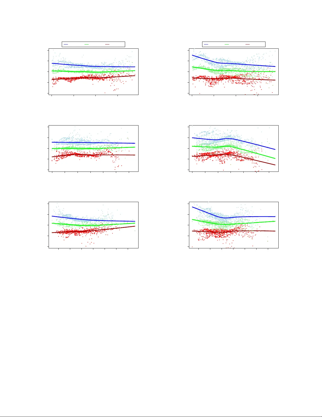
A nonparametric approac h to understand m ultiv ariate quan tile dynamics in ﬁnancial time series Kunal Rai 1 , Arc hi Roy 2 , Itai Dattner 3 , Soudeep Deb 1 1 Indian Institute of Management Bangalor e, Banner ghatta Main R d, Bangalor e, KA 560076, India. 2 Indian Institute of Scienc e Educ ation and R ese ar ch, Dr Homi Bhabha R d, Pune, MH 411008, India. 3 Dep artment of Statistics, University of Haifa, R abin Building, Mount Carmel, Haifa 3498838, Isr ael. Abstract: Ov er the last decade, nonparametric metho ds hav e gained increasing atten tion for modeling complex data structures due to their ﬂexibility and minimal structural assump- tions. In this pap er, w e study a general multiv ariate nonparametric regression framework that encompasses a broad class of parametric mo dels commonly used in ﬁnancial econometrics. Both the resp onse and the co v ariate pro cesses are allow ed to be m ultiv ariate with ﬁxed ﬁnite dimensions, and the framework accommodates temp oral dependence, thereby introducing ad- ditional mo deling and theoretical hurdles. T o address these c hallenges, w e adopt a functional dep endence structure which p ermits ﬂexible dynamic b ehavior while maintaining tractable asymptotic analysis. Within this setting, we establish strong and weak conv ergence results for the estimators of the conditional mean and volatilit y functions. In addition, we in vestigate conditional geometric quantiles in the multiv ariate time series context and prov e their consis- tency under mild regularit y conditions. The ﬁnite sample p erformance is examined through comprehensiv e simulation studies, and the metho dology is illustrated by mo deling the sto ck returns of Maersk and Lockheed Martin as a nonparametric function of a geop olitical risk index. Keyw ords and phrases: geometric quan tiles, Nadara y a-W atson estimator, sto c hastic re- gression, time series. 1. In tro duction Despite their widespread use in mo deling time series data, parametric framew orks hav e b een criti- cized for their limited ﬂexibility , particularly in some types of ﬁnancial datasets where they fail to capture the ric h and ev olving dynamics appropriately (see, for example, Bingham and Kiesel , 2002 ). This has spurred in terest in nonparametric metho ds, which oﬀer a ﬂexible and scalable alternative. In this pap er, our fo cus in this pap er is on a no vel extension of existing nonparametric theory whic h can b e useful in modeling and analyzing the dynamics of m ultiv ariate ﬁnancial data. Sp eciﬁcally , w e develop a uniﬁed nonparametric framework, along with suitable asymptotic theory , to explore the drift, volatilit y and quantiles in a multiv ariate time series. It is of essence here to recall that one of the earliest approaches in mo deling ﬁnancial returns nonparametrically was through con tinuous time diﬀusion mo dels (see Jiang and Knigh t , 1997 ; F an , 2005 , among others): d Y t = µ ( s t ) dt + σ ( s t ) dW t , where { Y t } is the series to b e mo deled as a function of a co v ariate { s t } , µ ( · ) and σ ( · ) are resp ectively the drift and the volatilit y function and { dW t } is a standard Brownian motion. In a nonparametric approach, no structural assumptions are imp osed on the functional forms of µ ( · ) and σ ( · ) functions; rather, they are globally estimated using a k ernel smo other. Notably , Zhao and W u ( 2008 ) established the asymptotic prop erties of these functional estimators in the univ ariate setting. How ever, extending this theory to a multiv ariate framew ork, esp ecially in the presence of temp oral dep endence, in tro duces substan tial tec hnical c hallenges, whic h 1 R ai et al. / Nonp ar ametric metho ds in multivariate ﬁnancial time series 2 w e address in this pap er. W e consider the mo del Y t = µ ( X t ) + Σ 1 / 2 ( X t ) e t , t = 1 , . . . , n, (1) where { Y t } ∈ R p represen ts a p -v ariate resp onse v ariable, { X t } ∈ X ⊆ R k is a k -dimensional co v ariate process with a compact X , and { e i } ∈ R p represen ts a m ultiv ariate stochastic indep enden t and identically distributed noise. Our theoretical results are deriv ed under the multi-dimensional case where p < ∞ and ﬁxed, and n → ∞ . F urther, our setup allows for b oth heavy-tailed and long memory in X t , making it esp ecially appropriate for application to ﬁnancial data. While we do not imp ose any parametric form on the functions µ : R k → R p and Σ : R k → R p × p , w e emphasize that ( 1 ) encompasses a large class of parametric mo dels commonly encountered in time series literature. F or example, putting µ ( x ) = A x and Σ( x ) = Σ for a constant matrix A ∈ R k × p and a p ositiv e deﬁnite matrix Σ ∈ R p × p , with X t = Y t − 1 giv es us the V AR(1) mo del. If X t further includes exogenous v ariables, then it is a V ARX mo del. Similarly , putting µ ( x ) = A 1 x 1 { x ∈R 1 } + A 2 x 1 { x ∈R 2 } with R 1 , R 2 b eing a partition of X , A 1 , A 2 ∈ R p × k and Σ( x ) = Σ , giv es us the m ultiv ariate threshold T AR model. A m ultiv ariate GARCH(1,1 ) mo del is obtained b y sp ecifying a constant (or linear) conditional mean and allowing the conditional co v ariance matrix to evolv e dynamically . F or example, we obtain a BEKK-GARCH type sp eciﬁcation by putting Σ( · ) = H t where H t = C + A 1 Y t − 1 Y ⊺ t − 1 A ⊺ 1 + B 1 H t − 1 B ⊺ 1 for matrices A 1 , B 1 , C of suitable dimensions. Similarly , other mo dels can also b e obtained b y suitably choosing the sp eciﬁcations. In subsequent sections, w e deﬁne the multiv ariate lo cal constant estimates of drift and volatilit y in the generalized framework ( 1 ), establish their consistency and w eak con vergence. Then, we fo cus on the estimation of conditional quan tiles, motiv ated b y their relev ance in ﬁnancial risk estimation. At this stage, it is natural to address why a m ultiv ariate notion of risk is required. In recen t y ears, m ul- tiv ariate risk measures ha ve attracted considerable attention since they explicitly accoun t for cross- sectional dep endence across assets. When tail b eha vior m ust b e assessed join tly for multiple ﬁnancial returns whose dep endence structure ev olv es with economic conditions, a vector-v alued conditional quan tile b ecomes essen tial. A motiv ating example for us is connected to modeling the join t lo wer-tail b eha vior of defense and transp ortation sto cks as a function of geop olitical risk indices, where sepa- rate univ ariate quantile estimates fail to capture the p ossibility of simultaneous extreme losses and the strengthening of dep endence during p erio ds of heigh tened geop olitical tension. A m ultiv ariate conditional quantile, returning a vector of the same dimension as the resp onse, provides a coherent ob ject that captures b oth marginal tail b eha vior and their joint structure. Empirical evidence, such as Santos, Nogales and Ruiz ( 2013 ), suggests that m ultiv ariate approac hes outp erform univ ariate metho ds in p ortfolio v alue-at-risk ev aluation. In this context some early contributions (e.g. Jouini, Meddeb and T ouzi , 2004 ; Ek eland, Galic hon and Henry , 2012 ; Cousin and Di Bernardino , 2013 ) prop osed v arious multiv ariate risk measures, which were later criticized for lac king clear economic in terpretation. Recen t con tributions include order-statistic and quan tile-regression–based methods ( Ch un, Shapiro and Uryasev , 2012 ; Sun, W ang and Y u , 2018 ), copula-based constructions ( Coblenz, Dyc kerhoﬀ and Grothe , 2018 ), and optimal-transp ort–based quantiles ( Bercu, Bigot and Thurin , 2024 ). In this study , w e adopt geometric quantiles ( Chaudhuri , 1996 ; Cho wdhury and Chaudhuri , 2019 ), whic h provide a natural and well-deﬁned m ultiv ariate extension of univ ariate quantiles with- out requiring an ordering in higher dimensions. Deﬁned through a conv ex optimization problem, geometric quantiles enjo y uniqueness under mild conditions, are aﬃne equiv ariant, and retain a direct connection to classical univ ariate quantile regression ( Koenker and Bassett Jr , 1978 ). This mak es them particularly suitable for conditional multiv ariate time series mo deling. Ov erall, the contribution of this pap er is three-fold. First, we use Nadaray a-W atson t yp e non- parametric metho ds for estimating multiv ariate conditional mean and v ariance and deriv e suitable R ai et al. / Nonp ar ametric metho ds in multivariate ﬁnancial time series 3 asymptotic theory whic h has not b een formally done b efore. Second, we prop ose a nonparametric metho dology for estimating conditional geometric quan tiles of multiv ariate time series, where the resulting quan tile is vector-v alued and matches the dimension of the resp onse. Relev an t asymptotic prop erties of the prop osed conditional quantile estimator are derived under mild regularity con- ditions, allowing for hea vy-tailed inno v ations and general dep endence structures in the cov ariates. Ov erall, this provides an integrated treatment of lo cation, scale, and tail b eha vior for multiv ariate ﬁnancial data. As the third contribution of this pap er, we pro vide detailed empirical exploration of the dev elop ed theory with a real-life study on the b eha vior of tw o imp ortant geop olitical risk-prone sto c ks – Lockheed Martin, whic h is a defense company in United States of America, and Maersk, whic h is a shipping company in Denmark – under the inﬂuence of the geopolitical risk. A sim ulation study that mimics similar time series data is also included in the pap er for completeness. The rest of the article is organized in the following manner. W e review relev ant literature in Section 2 . The main theoretical results p ertaining to the asymptotic theory of the drift, volatilit y and quantile estimates are established in Section 3 . The eﬃcacy of the prop osed estimators are illustrated with a brief sim ulation study and a detailed real data application on defense and shipping mark ets in Section 4 and Section 5 , resp ectively . Finally , we conclude with some necessary remarks in Section 6 . In the interest of space, all pro ofs are deferred to the App endix. 2. Literature Review A v ast literature has dev elop ed on nonparametric regression for estimating the conditional mean function µ ( · ) . Standard approac hes include lo cal constant, lo cal linear, and lo cal p olynomial es- timators, along with robust v ariants suc h as nonparametric M-estimators and smo othing splines. Early methodological contributions include design-adaptive regression ( F an , 1992 ), nearest-neighbor metho ds ( Altman , 1992 ), and regression with noisy co v ariates ( Mammen, Rothe and Schienle , 2012 ). Theoretical properties of these estimators are w ell understo od in the independent data setting ( T akeza wa , 2005 ), while extensions to higher-dimensional settings hav e largely relied on sparsity assumptions or v ariable selection tec hniques ( Lin and Zhang , 2006 ; Bertin and Lecué , 2008 ; Y ang and T okdar , 2015 ). In contrast, we consider multiv ariate nonparametric regression in a time series framew ork with temp oral dep endence and without imp osing sparsit y restrictions. Compared to the literature of conditional mean estimation, there hav e b een less work dev oted to the estimation of the conditional volatilit y . Early contributions in this direction include Müller and Stadtmüller ( 1987 ); Hall, Ka y and Titterington ( 1990 ), among others. These studies primarily fo cused on estimating the conditional v ariance as a single scalar quan tity , rather than mo deling it as a function of the cov ariate pro cess. A particularly inﬂuen tial con tribution is W ang et al. ( 2008 ), whic h established minimax optimal rates for the estimation of conditional heteroskedasticit y in nonparametric regression settings. In con text of estimation of the conditional v ariance function, Chib, Nardari and Shephard ( 2006 ) prop osed a Bay esian approac h based on Mark ov c hain Mon te Carlo sampling from standard distributions, dra wing inspiration from techniques developed for the estimation of sto chastic volatilit y mo dels, as illustrated in Kim, Shephard and Chib ( 1998 ). An inno v ative approach was prop osed b y Cai and W ang ( 2008 ), who dev elop ed a data-driven estimator of the conditional heterosk edasticity function by applying w av elet thresholding to the squared ﬁrst- order diﬀerences of the observ ations. P arallel approaches to the estimation of the conditional v ariance include least squares–based estimators ( T ong and W ang , 2005 ), metho ds based on w eighted empirical pro cesses ( Cho wn and Müller , 2018 ), techniques employing second-order U-statistics ( Liu et al. , 2021 ), and more recent approaches based on v ariational mo de decomp osition ( P alanisamy , 2017 ). While most of these techniques can b e adapted to m ultiv ariate data, they are largely reliant on the data generating pro cess being indep endent. In Kulik and Wic helhaus ( 2011 ), the authors considered R ai et al. / Nonp ar ametric metho ds in multivariate ﬁnancial time series 4 the heteroskedasticit y estimation problem for nonparametric regression with dep enden t errors, and more recently Hu ( 2013 ) prop osed a k ernel-based estimator which retained asymptotic consistency under strongly mixing in the data generating pro cess. Complemen ting the existing literature, we prop ose estimation of the conditional v ariance under v ery general structure of the m ulti-dimensional co v ariate pro cess, which cov ers the case of b oth short and long memory . W e further establish their asymptotic consistency and weak conv ergence prop erties under minimal structural assumptions. T urning atten tion to the estimation of multiv ariate quan tiles, we note the parametric and semi- parametric approac hes of Chakrab ort y ( 2003 ); Ma et al. ( 2019 ); Jureč ko v á, Picek and Kalina ( 2024 ), while nonparametric extensions of lo cal linear metho ds for real-v alued resp onses app ear in Lejeune and Sarda ( 1988 ); Y u and Jones ( 1998 ); Horowitz and Lee ( 2005 ). Ho w ever, these metho ds are primarily designed for scalar resp onses and do not directly address genuinely m ultiv ariate quantile ob jects. More recent work on multiv ariate quantiles includes directional, kernel-based, copula-based, and conditioning-based constructions; see Chav as ( 2018 ), Huang and Nguy en ( 2018 ), Coblenz, Dy- c kerhoﬀ and Grothe ( 2018 ), and Galv ao and Montes-Ro jas ( 2025 ). Our approach instead builds on the geometric quantile framework, which formulates m ultiv ariate quantiles through a conv ex opti- mization problem and a voids the need for ordering, conditioning sequences, or dimension-reduction sc hemes. Unlike muc h of the existing literature, whic h is developed under indep endence or struc- tured mo del assumptions, we establish asymptotic results for conditional geometric quantiles in a m ultiv ariate time series setting with general dep endence. This places multiv ariate quantile estima- tion within a fully nonparametric dynamic framework and complements the existing b ody of w ork on mean and v ariance estimation under dep endence. 3. Metho dology Throughout this article, the sym b ols R , Z , L k are used to indicate resp ectiv ely the set of real num- b ers, the set of in tegers, and the set of all random v ariables with ﬁnite moments up to the k th order. Whenev er used, I represents an identit y matrix of appropriate order. Otherwise, b old-faced letters are used to denote v ectors unless otherwise stated. W e shall use D − → (similarly , P − → ) to indi- cate conv ergence in distribution (similarly , con vergence in probabilit y). Finally , N p ( θ , Σ) refers to a p -v ariate Gaussian distribution with mean θ and co v ariance matrix Σ . 3.1. Mathematic al fr amework Recall our stochastic regression mo del describ ed in ( 1 ) that cov ers a wide v ariety of commonly encoun tered multiv ariate time series models. W e ﬁrst deﬁne the problem setting in whic h our uniﬁed approac h of multiv ariate nonparametric estimation of conditional mean, v ariance, and quantiles is dev elop ed. The cov ariate pro cess { X t } is tak en to be stationary and independent of the error pro cess { e t } . It is deﬁned through a measurable function of an indep endently and identically distributed (iid) sequence of random v ariables { η t } t ∈ Z as X t = G ( F t ) , (2) where F t is the σ -ﬁeld generated by ( . . . , η t − 1 , η t ) , and G is a measurable function such that X t is well deﬁned. Suc h an assumption is commonly used in time series literature; see F an ( 2005 ) for a detailed review. As an example to illustrate this data generation pro cess, let X i = c + P q j =1 B j ε i − j + ε i where ε i − j is a past white noise vector of index i − j , c is a vector of constan ts, B j are matrices of co eﬃcien ts for each lag j and ε i is a vector of error terms. T o capture the dep endence structure in { X t } w e deﬁne a pro jection op erator P k , whic h for a random v ariable W ∈ L 1 and for k ∈ Z , is R ai et al. / Nonp ar ametric metho ds in multivariate ﬁnancial time series 5 deﬁned as: P k W = E ( W | F k ) − E ( W | F k − 1 ) . Denote F X and F e as the multiv ariate distribution functions of X 0 and e 0 resp ectiv ely; with f X = F ′ X and f e = F ′ e b eing the corresp onding density functions. F urther, for i ∈ Z , let F X ( x | F i ) = P ( X i +1 ⩽ x | F i ) denote the m ultiv ariate conditional distribution function of X i +1 giv en F i and f X ( x | F i ) = ∂ F X ( x | F i ) /∂ x the corresp onding conditional densit y . Then, following W u ( 2005 ), deﬁne the functional dep endence measure θ i = sup x ∈ R k [ ∥P 0 f X ( x | F i ) ∥ +   P 0 f ′ X ( x | F i )   ] , (3) where f ′ X ( x | F i ) = ∂ f X ( x | F i ) /∂ x , if it exists. Roughly , the term θ i measures the contribution of e 0 in predicting X i +1 . Using this, for n ∈ N , we further deﬁne Θ n = n X i =1 θ i , Λ n = n Θ 2 2 n + ∞ X k = n (Θ n + k − Θ k ) 2 . (4) W e consider Θ ∞ < ∞ , whic h implies that the cum ulative contribution of η 0 in predicting future v alues is ﬁnite, th us pointing to the short-range dep endence (SRD) setting. In this case, Λ n = O ( n ) . When Θ ∞ → ∞ , we hav e the long range order. 3.2. Estimation pr o c e dur e and asymptotic the ory for c onditional me an and volatility T o establish the theoretical properties of the estimates in ( 5 ) and ( 6 ), w e b egin by introducing some notation of future interest. Let C 0 ( x ) denote a set of con tinuous functions in the ϵ -neigh b orho o d of x , deﬁned as x ϵ = S y ∈ R k { y : ∥ x − y ∥ ⩽ ϵ } ∈ R k for some ϵ > 0 . Next, deﬁne C N ( x ϵ ) := { g ( · ) : sup x ∈ x ϵ | g ( l ) ( x ) | < ∞ , for l = 0 , . . . , N ∈ Z } as the set of all the functions that hav e b ounded deriv ativ es on x ϵ up to N . The density function f X is assumed to satisfy the conditions f X > 0 and f X ∈ C 2 ( { x ϵ } ) for all ϵ satisfying ∥ ϵ ∥ > 0 . Next, w e assume e t ∈ L 2 , where a random v ariable W is considered to be in L p for p > 0 , if ∥ W ∥ p := [ E ( | W | p )] 1 /p < ∞ . In the same context, denote V e = v ar [ e t ] . Finally , let K b e the set of kernels which are symmetric, whose v alues are b ounded, and ha v e bounded deriv ativ e and b ounded supp ort. The kernel functions used in our metho ds are considered to b e tak en from this set. Using ⟨· , ·⟩ to indicate inner pro ducts, tw o terms of in terest, ψ K and ϕ K , are deﬁned as ψ K = 1 2 R R k ⟨ t , t ⟩ K ( t ) d t and ϕ K = R R k K 2 ( t ) d t . The mo del ( 1 ) explores relationships among v arious co v ariates and the m ulti-dimensional dep en- den t v ariable through the mean function µ ( · ) , and the conditional v ariance function Σ( · ) . W e let µ, Σ ∈ C 2 ( { x } ϵ ) for all ϵ satisfying ∥ ϵ ∥ > 0 , along with Σ( x ) b eing a p ositiv e deﬁnite matrix for all x . W e also assume that our time series v ariables are stationary and E [ ∥ Y 0 ∥ 4 ] < ∞ . W e use nonpara- metric Nadaray a-W atson ty p e estimators to estimate these functions. It is imp erative to p oin t out that a lo cal constant estimator instead of lo cal linear estimator is attractiv e due to mathematical prop erties, how ever the asymptotic theory follows in similar lines with sligh t mo diﬁcations. The estimator for the multiv ariate mean and v ariance function are resp ectively given by b µ ( x ) = n X t =1 Y t ν t ( x ) , (5) and b Σ( x ) = n X t =1 ( Y t − b µ ( X t )) ν t ( x ) ( Y t − b µ ( X t )) ⊺ , (6) where ν t ( x ) = K b n ( x − X t ) P n t =1 K b n ( x − X t ) , K b n ( v ) = 1 b k n K  v b n  . (7) R ai et al. / Nonp ar ametric metho ds in multivariate ﬁnancial time series 6 In the ab ov e, K : R k → R is an appropriately chosen k ernel function and b n is the bandwidth satisfying b n → 0 and nb n → ∞ as n → ∞ . F or notational ease, we shall use the same bandwidth b n throughout this pap er, although each estimator can also b e computed using diﬀeren t bandwidth c hoices, with minimal mo diﬁcations to the theory . No w, the following theorem establishes the consistency and the asymptotic Gaussian b eha vior of the p oin twise estimate of conditional mean under certain bandwidth conditions. Theorem 1. i) F or any ﬁxe d x ∈ R k , under the afor ementione d settings, the pr op ose d estimate of the me an function c onver ges to the p opulation e quivalent in pr ob ability, i.e., b µ ( x ) P − → µ ( x ) . ii) F urther assume the b andwidth satisﬁes b n + nb k +4 n + 1 nb k n + Λ n  b 3 n n + 1 n 2  → 0 , (8) and let ρ µ ( x ) = ∇ 2 µ ( x ) + 2 ∇ µ ( x ) ∇ f X ( x ) f X ( x ) . Then as n → ∞ , q nb k n ˆ f X ( x ) √ ϕ K (Σ 1 / 2 ( x ) V e Σ 1 / 2 ( x ) ⊤ ) − 1 / 2 ( x )  b µ b n ( x ) − µ ( x ) − b 2 n ψ K ρ µ ( x )  D − → N p ( 0 , I ) . (9) The ﬁrst part of the pro of of Theorem 1 follows from the T aylor expansion of the nonparametric estimate. The asymptotic distribution is derived by expressing ( b µ ( x ) − µ ( x )) as a martingale diﬀer- ence sequence; follow ed by an application of the martingale central limit theorem. The details, for brevit y , are added in the App endix. Note from mo del ( 1 ) that the conditional co v ariance matrix of Y t giv en X t = x is Υ( x ) := V ar ( Y t | X t = x ) = (Σ 1 / 2 ( x ) V e Σ 1 / 2 ( x ) ⊤ ) , whic h appears as the scaling factor in the abov e asymptotic distribution. W e hereafter suppose, V e = I for the purpose of brevit y and conv enience, similar results can b e established with a general, V e , as well. Note that if V e = I then Υ( x ) = Σ( x ) . The next result establishes the consistency of the v ariance function. It allo ws us to substitute the p opulation conditional v ariance function by a sample estimate, as discussed b elo w. Theorem 2. F or any ﬁxe d x ∈ R k , under the afor ementione d settings, the pr op ose d estimate of the c ovarianc e function c onver ges to the p opulation e quivalent in pr ob ability, i.e., b Σ( x ) p → Σ( x ) . The pro of of Theorem 2 uses the oracle estimator e Σ and compares it to the Nadara y a W atson based estimator b Σ , subsequen tly connecting it to the true co v ariance function, Σ . The details are deferred to the App endix. It further helps us in obtaining the following result. Corollary 1. F or signiﬁc anc e level α , a 100(1 − α )% c onﬁdenc e interval for line ar functional of the form a ⊺ µ, a ∈ R p , is obtaine d as a ⊺ µ ( x ) ∈ a ⊺ b µ ∗ b n ( x ) ± s ϕ K nb k n ˆ f X ( x ) χ 2 p ;1 − α a ⊺ b Σ( x ) a . (10) The ab ov e gives us a band that cov ers all p ossible linear contrasts. Here, following standard lit- erature, b µ ∗ b n ( x ) is a jac kknife-t yp e estimator to provide bias-corrected m ultiv ariate mean estimate. Note that setting a equal to empirical basis vectors w ould yield marginal interv als for each com- p onen t µ j ( x ) with family-wise cov erage 1 − α . Corollary 1 is straightforw ard from the results of Theorem 1 , part ( ii ) , Theorem 2 , and Slutsky’s theorem. Estimation of the conditional mean function in ( 1 ) c haracterizes the expected or a verage behavior of the resp onse v ariable given the cov ariates. F or a sample of size n and co v ariate dimension p , the R ai et al. / Nonp ar ametric metho ds in multivariate ﬁnancial time series 7 conditional mean of the dep enden t v ariable is expressed in ( 5 ), where the asso ciated weigh ts are deﬁned in ( 7 ). Beyond mo deling the av erage b ehavior, the framew ork also allows estimation of the conditional v ariance function which captures the time-v arying disp ersion of the resp onse v ariable. T ogether, these tw o comp onen ts describ e b oth the exp ected return and the asso ciated uncertaint y conditional on av ailable information. In ﬁnancial applications, this distinction is particularly im- p ortan t. The conditional mean provides insight into exp ected returns or price mov emen ts, while the conditional v ariance reﬂects risk or volatilit y . Accurate estimation of b oth functions enables impro ved forecasting, p ortfolio allo cation, and risk management, as inv estors require not only pre- dictions of a verage performance but also reliable measures of the v ariabilit y and p oten tial do wnside risk surrounding those predictions. W e prop ose to use multiv ariate Epanechnik ov or parab olic kernel function. It is b ounded on its supp ort, the p -dimensional unit ball, and is given by: K ( u ) = k + 2 2 c k (1 − u ⊺ u ) I ( ∥ u ∥ ⩽ 1) , (11) where c k = π k/ 2 / Γ( k 2 + 1) is deﬁned through the gamma function, and ∥ u ∥ = q P k i =1 u 2 i . The purp ose of using a k ernel function with a b ounded supp ort in this case is the computational ease that it oﬀers. W e ma y also use kernels with no b ounded supp ort, such as the m ultiv ariate gaussian k ernel function, and the p erformance will remain similar. 3.3. Estimation pr o c e dur e and asymptotic the ory for c onditional quantiles W e adopt the geometric quantile deﬁnition to estimate the m ultiv ariate quantiles following the form ulation proposed b y Chowdh ury and Chaudhuri ( 2019 ). The use of geometric quan tiles stems from its theoretical prop erties, including existence, uniqueness, and strict con v exity of the ob jective function as w ell as empirical usefulness in capturing directional features of m ultiv ariate distributions. Geometric quan tiles provide a coherent and non crossing c haracterizations indexed b y direction v ectors. W e ﬁrst deﬁne p opulation v ersion of the conditional geometric quan tile of Y t giv en the co v ariate X t = x is deﬁned as Q ( u , x ) := arg min q ∈ R p M ( p ) u ( q ); where, M ( p ) u ( q ) := E [ || Y t − q || + ⟨ u | S p Y t − q ⟩ | X t = x ] , (12) F urther, we deﬁne the conditional quantiles for sample based on the deﬁnition for p opulation, ˆ q n ( u , x ) := arg min q ∈ R p M ( p ) u ,n ( q ); where, M ( p ) u ,n ( q ) := 1 n n X t =1 {∥ Y t − q ∥ K b n ( · ) + ⟨ u | Y t − q ⟩ K b n ( · ) } . (13) The minimization problem in volv ed in ( 13 ) is non-trivial. W e prop ose using an iterativ ely re- w eighted least squares (IRLS) estimation tec hnique, which oﬀers an eﬃcien t metho d for the es- timation of the required quantiles. The key up dating step of the minimization algorithm is giv en as ˆ q ( k +1) n ( u , x ) = 1 2 P n t =1 K b n ( X t − x ) u + P n t =1 w t ( ˆ q ( k ) ) K b n ( X t − x ) 2 Y t P n t =1 w t ( ˆ q ( k ) ) K b n ( X t − x ) 2 , (14) where w t ( q ( k ) ) = ∥ Y t − ˆ q ( k ) n ( u | x ) ∥ − 1 K b n ( x − X t ) is a sequence of weigh ts. The following theorem establishes b oth the algorithmic stability and the structural c haracteri- zation of the geometric quan tile estimator. It ﬁrst demonstrates the n umerical conv ergence of the IRLS sc heme b y utilizing its descent prop ert y to show that the sequence of iterates conv erges to the R ai et al. / Nonp ar ametric metho ds in multivariate ﬁnancial time series 8 unique global minimizer of the ob jective function. This guarantees the stability of computation and the v alidit y of the algorithmic implementation. In addition, the theorem pro vides the ﬁrst order op- timalit y condition satisﬁed by the sample minimizer and its corresp onding p opulation counterpart. In this w ay , it links the computational pro cedure to the underlying theoretical structure, establishes the existence and uniqueness of the minimizer, and connects the sample and p opulation geometric quan tiles through their resp ectiv e estimating equations. Theorem 3. Assume that for e ach ac cumulation p oint ¯ q of the IRLS iter ates { q ( k ) } k ⩾ 0 , ther e exists a c onstant δ > 0 (indep endent of n and p ) such that min 1 ⩽ t ⩽ n ∥ Y t − ¯ q ∥ K ( · ) ⩾ δ . Under the pr eviously state d r e gularity assumptions and the b andwidth c ondition, the IRLS scheme deﬁne d thr ough ( 14 ) pr o duc es a se quenc e of iter ates whose obje ctive values { M ( p ) u ,n ( q ( k ) ) } k ⩾ 0 ar e non incr e asing, and the iter ates q ( k ) c onver ge to the unique glob al minimizer ˆ q n ( u , x ) of the obje ctive function M ( p ) u ,n . Mor e over, the sample minimizer ˆ q n ( u , x ) satisﬁes the ﬁrst or der optimality c ondition n X t =1 K b n ( X t − x )  Y t − ˆ q n ( u , x ) ∥ ( Y t − ˆ q n ( u , x )) ∥ + u  = 0 . (15) The p opulation quantile Q ( u , x ) , deﬁne d as the minimizer of the p opulation obje ctive M ( p ) u , sat- isﬁes the c orr esp onding p opulation version E Y i | X i = x  Y i − Q ( u , x ) ∥ Y i − Q ( u , x ) ∥ + u  = 0 . (16) In implementations one ma y , instead of w t ( q ( k ) ) , use stabilized w eights w t,ϑ ( q ) = 1 / ( ∥ Y t − q ∥ K ( · ) + ϑ ) with a small ﬁxed ϑ > 0 to av oid n umerical instability when an iterate approaches a data p oin t. The conv ergence argument ab o ve is stated for ϑ = 0 under the separation assumption, while the stabilized version corresp onds to minimizing a smo oth p erturbed ob jective and enjo ys the same monotone descen t prop ert y . Corollary 2. Assume that for e ach ﬁxe d x ∈ X the p opulation obje ctive M ( p ) u ( q ) is strictly c onvex in q and admits a unique minimizer Q ( u , x ) . Then, for e ach ﬁxe d x , the mapping u 7→ Q ( u , x ) wher e u ∈ B p − 1 , is inje ctive. In p articular, if u 1  = u 2 , then Q ( u 1 , x )  = Q ( u 2 , x ) , and henc e the ge ometric quantiles p ossess an intrinsic non cr ossing structur e acr oss dir e ctions. In the geometric quan tile framew ork, quan tiles are indexed by directions u ∈ B p − 1 rather than b y a scalar level. F or each ﬁxed x , the geometric quantile Q ( u , x ) is deﬁned as the unique minimizer of a strictly conv ex ob jectiv e. Strict conv exit y ensures uniqueness for each ﬁxed u . T o establish the non crossing prop erty across directions, consider the p opulation ﬁrst order con- dition satisﬁed by the geometric quantile: E  Y − Q ( u , x ) ∥ Y − Q ( u , x ) ∥    X = x  = − u . Supp ose, for contradiction, that tw o distinct directions u 1  = u 2 pro duce the same quantile q = Q ( u 1 , x ) = Q ( u 2 , x ) . Then the ﬁrst order condition would imply E  Y − q ∥ Y − q ∥    X = x  = − u 1 and E  Y − q ∥ Y − q ∥    X = x  = − u 2 , whic h is imp ossible since u 1  = u 2 . Therefore, distinct directions m ust pro duce distinct quan tiles. This establishes mapping is injective, and hence the geometric quantiles p ossesses an intrinsic non crossing structure. R ai et al. / Nonp ar ametric metho ds in multivariate ﬁnancial time series 9 The following result establishes consistency of our multiv ariate quan tile estimator by sho wcasing the conv ergence of the sample estimate, ˆ q n ( u , x ) , to the population estimate, Q ( u , x ) in probability hence reinforcing the b eliev e in the accuracy of our estimator as the num b er of observ ations increases. Theorem 4. Under the pr evious assumptions on quantile estimates and b andwidth, the estimator ˆ q n ( u , x ) of the p opulation quantile Q ( u , x ) , satisﬁes ∥ ˆ q n ( u , x ) − Q ( u , x ) ∥ = O P ( q p/nb k n ) , (17) for al l x ∈ X wher e X ⊂ R k is c omp act and R X ∥ u ( s ) ∥ 2 ds ⩽ 1 . In establishing the ab ov e result w e utilize the analytical stability result from Theorem 3 , the strict con vexit y of the ob jectiv e function, and rates of con v ergence for the relev ant terms in the T aylor expansion of the score function under the small range dep endence in the ph ysical dep endence setting Λ n = O ( n ) . Estimation of the conditional quantile function, from ( 1 ), giv es us the av erage percentile b eha vior of the response v ariable. F or n num b er of observ ations and p num b er of dimensions, the conditional quan tile of the dep enden t v ariable, conditioned on the cov ariates is given b y Equation ( 14 ) where a mo diﬁed pinball-t yp e loss function for the multiv ariate case is used. The expression, ∥ Y t − q ∥ is a norm, and the expression, ⟨ u , Y t − q ⟩ K ( · ) , describ es an euclidean inner pro duct b etw een u and Y t − q under kernel function, K ( · ) . The expression for Q ( u ) is a generalization of the ob jective function deﬁned by Koenker and Bassett Jr ( 1978 ). Man y of the risk measures are deriv ativ e of the quantiles, example, V alue-at-Risk and A verage V alue-at-Risk. W e emphasize on the V alue-at-Risk measure whic h has b een established as an impor- tan t ﬁnancial risk measure p ost the 2008 ﬁnancial crisis, (see Ruiz and Nieto ( 2023 ). V alue-at-Risk (V aR) at conﬁdence level α ∈ (0 , 1) is the α -quantile of the loss distribution. Supp ose L denotes loss, then, V aR α = inf { l ∈ R : P ( L ⩽ l ) ⩾ α } . (18) A t level α , V aR is the smallest n umber l suc h that the probability of the loss exceeding l is at most 1 − α . 4. A short sim ulation study W e conduct a brief sim ulation study that replicates real-world phenomena, particularly a multiv ari- ate time series data with temp oral dep endence among resp onse v ariables, likely to app ear in the w orld of ﬁnance. This study is primarily designed to establish ﬁnite sample b ehavior and empirical consistency . This exercise enables us to examine the generalized sto c hastic regression framework that w e are working with, as well as the accuracy of the estimation pro cedure. The sim ulation setup is established by deﬁning the data-generating pro cesses and sp ecifying the num b er of ob- serv ations. W e consider three co v ariates ( k = 3 ), denoted as X t = { X 1 ,t , X 2 ,t , X 3 ,t } , and explore diﬀeren t t yp es of data generation. In this simulation study , we ev aluate the estimation accuracy of the multiv ariate conditional means and multiv ariate conditional quantiles, which are the main fo cus of the current study . The estimation of multiv ariate conditional v ariance is primarily explored as an auxiliary comp onen t required for inference, including asymptotic v ariance characterization and construction of conﬁdence regions of the mean. The cov ariates in the simulation study are generated under autoregressive pro cesses of order 1 with common innov ations whic h induce serial correlation and con temp oraneous dep endence among the v ariables. The resp onse v ariables Y = { Y 1 , Y 2 } (i.e., R ai et al. / Nonp ar ametric metho ds in multivariate ﬁnancial time series 10 p = 2 ) are generated follo wing the sp eciﬁcations Y 1 t = 1 3 ( X 1 t + X 2 t + X 3 t ) + e 1 t , Y 2 t = b 1 X 1 t + b 2 X 2 t + b 3 X 3 t + e 2 t ; with 3 X i =1 b i = 1 . These t w o dependent response v ariables with distinct dependence structure on the co v ariates helps in exhibiting the strength of our metho dology . The error comp onents e 1 t , e 2 t for all timep oin ts are sim ulated indep endent ly using three diﬀerent p opulation distributions: standard normal, student’s t with 3 degrees of freedom, and shifted exp onen tial. These choices are made to ensure that they co ver light tail, heavy tail, and skew ed error designs, resp ectiv ely . The sample sizes are tak en as n ∈ { 100 , 500 , 1000 } , representing small, mo derate and large sample regimes. F ollowing the metho dology described in Section 3 , we apply the estimation techniques for diﬀerent conditional functions, and compare our estimates with the true v alues that can b e obtained b y Mon te Carlo sampling from the conditional distributions in our data generating pro cesses. F or the quan tiles, we consider ﬁv e diﬀerent levels: 0.05, 0.1, 0.5, 0.9, and 0.95. A t each quantile lev el, w e use IRLS scheme to obtain the geometric multiv ariate quantiles as explained in Section 3.3 . The directional vector u ∈ B p − 1 is c hosen appropriately in this regard. The bandwidth selection for the conditional mean estimation is carried out using a blo ck ed cross-v alidation pro cedure for time series data, while for the conditional quan tile estimation a rate-consisten t bandwidth c hoice is used. W e replicate this exercise for 50 Mon te Carlo iterations and compute the ro ot mean square error (RMSE) to assess the accuracy of our metho dology . While it is our primary accuracy metric, we also rep ort mean absolute p ercen tage error (MAPE) in a relativ e scale, which provides us a scale-free measure to identify ho w the accuracy is improving based on the sample size. In this regard, the baseline is kept at n = 100 for each case. The simulation results are tabulated b elow. In T able 1 , w e see that for each error distribution considered, the t wo metrics display a visibly evident decreasing pattern with increasing sample sizes. This suggests an empirical consistency for the multiv ariate conditional mean estimates. T able 2 , on the other hand, illustrates the p erformance of the conditional quantile estimates for diﬀerent sample sizes, quantile lev els and error distributions. Here also, the results suggest empirical consistency for the m ultiv ariate conditional quan tile estimates for each quantile level. T able 1 Simulation r esults for multivariate c onditional me an estimation. Sample size ( n ) Error distribution RMSE Relative MAPE 100 Normal 0.259 1.000 500 Normal 0.141 0.529 1000 Normal 0.111 0.292 100 Exp onen tial 0.250 1.000 500 Exp onen tial 0.135 0.212 1000 Exponential 0.105 0.157 100 t 3 0.362 1.000 500 t 3 0.203 0.669 1000 t 3 0.158 0.400 5. Application As a practical illustration, w e study the intricate relationship b etw een the log-return series of the sto c k market data of Maersk and Lo c kheed Martin with geop olitical risk. Using the prop osed uniﬁed R ai et al. / Nonp ar ametric metho ds in multivariate ﬁnancial time series 11 T able 2 Simulation r esults for multivariate c onditional quantiles estimation. Sample Quan tile Normal error Exp onen tial error t 3 error size ( n ) ( τ ) RMSE Relativ e MAPE RMSE Relativ e MAPE RMSE Relativ e MAPE 100 0.05 0.304 1.000 0.222 1.000 0.432 1.000 500 0.05 0.173 0.834 0.119 0.624 0.227 0.097 1000 0.05 0.139 0.491 0.083 0.328 0.173 0.046 100 0.10 0.300 1.000 0.227 1.000 0.421 1.000 500 0.10 0.172 0.485 0.121 0.464 0.224 0.378 1000 0.10 0.138 0.389 0.085 0.340 0.170 0.321 100 0.50 0.290 1.000 0.270 1.000 0.384 1.000 500 0.50 0.166 0.710 0.148 0.568 0.212 0.358 1000 0.50 0.135 0.540 0.108 0.513 0.159 0.212 100 0.90 0.299 1.000 0.335 1.000 0.421 1.000 500 0.90 0.169 0.418 0.190 0.328 0.219 0.575 1000 0.90 0.138 0.401 0.141 0.271 0.174 0.414 100 0.95 0.303 1.000 0.345 1.000 0.429 1.000 500 0.95 0.169 0.873 0.197 0.186 0.223 0.767 1000 0.95 0.139 0.437 0.147 0.153 0.180 0.585 estimation technique, we ev aluate the conditional prop erties in a multiv ariate sense, sp eciﬁcally v arious magnitudes of risk through quantiles. It is of the essence here to recall few studies that fo cused on defense and shipping sto ck markets. Shac kman et al. ( 2021 ) examined ho w the global maritime stock prices aﬀect the stock prices of large transportation companies. Bhattac harjee ( 2022 ) analyzed the v olatility of the defense sto cks, while the work of Stanivuk, Lalić and Amižić ( 2023 ) assesed the impact of w ar in Ukraine on the shipping industry using parametric techniques. Most recen tly , Sim et al. ( 2024 ) studied the relationship of global supply chain pressure index and sto c k prices of global logistic companies. In our illustration, as co v ariates we use three types of geop olitical risk indices introduced by Caldara and Iacoviello ( 2022 ). The authors derive these indices using newspap er co verage of even ts lik e war, terror attacks, and other even ts of global relev ance such as election results of ma jor coun- tries. The geop olitical risk index not only captures the actual even ts of disruptions but also any sp eculations. More than 25 million news articles from ma jor English newspap ers are used in this regard. Roughly sp eaking, a ratio of the num b er of articles with sp eciﬁc w ords whic h correlates hea vily with geop olitical risks to the total num b er of articles is used to compute the risk index. There are three indices prop osed: the ﬁrst one captures the ov erall geop olitical risk, the second one is an act based geop olitical risk index that realizes disruptions in the geop olitical relationships, and the third one is a threat based geop olitical risk index that anticipates disruptions in the geop olitical relationships. These three indices are hereafter denoted as GPRD, GPRD-A, and GPRD-T, resp ec- tiv ely . As our resp onse v ariables, we use log-returns of the stock prices of Lockheed Martin, a global defense compan y ( Y LHM ), and Maersk, a global shipping company ( Y MMA ). The timeline of the data is the p erio d from 1st April, 2021 to 31st March, 2025. This timeline whic h is marked as a recov ery p erio d from m ultiple CO VID-19 wa ves, is also kno wn for other globally consequen tial even ts lik e the Russia-Ukraine conﬂict, T urk ey-Syria earthquake, Nagorno-Karabakh conﬂict escalation, Civil war in Sudan and the Israel-P alestine conﬂict, just to name a few. A few exploratory plots are presented in Section B in the interest of space. First, Figure B.1 shows the geop olitical risk indices against time: the ev ents of Russia-Ukraine conﬂict (RUC) in F ebruar y 2022 and Israel-Palestine conﬂict (IPC) in Octob er 2023 are particularly visible via p eaks in all three R ai et al. / Nonp ar ametric metho ds in multivariate ﬁnancial time series 12 time series plots, and they will b e of particular interest to us. On the other hand, Figure B.2 sho ws the sto ck prices, log-returns, and volatilit y of the tw o sto cks. The top tw o panels show a consistent increasing trend in LHM whereas MMA observ es an increasing trend from April 2021 to Jan uary 2022, but a decreasing trend afterw ard. The av erage log-returns for b oth sto c ks generally stay close to zero, with o ccasional ﬂuctuations, as displa yed in the middle tw o panels. Finally , the v olatility series display ed in the b ottom tw o panels are based on 5-da y rolling standard deviation and are represen tatives of the risk asso ciated with these sto cks. The LHM sto ck shows t w o p erio ds of high v olatility (2022-23 and 2024-25) and tw o perio ds of low volatilit y (2021-22 and 2023-24). The MMA sto c k, comparatively sp eaking, observes high volatilit y throughout the p erio d of study with tw o exceptional p eaks during the RUC and in the early months of 2024, p ossibly caused b y the IPC. F or the main analysis, w e apply our prop osed techniques of analyzing m ultiv ariate conditional mean, v ariance, and quantiles. W e discuss these resul ts in the same order with other analyses wherev er suited for clarit y and coherence. F or implementation, w e use cross-v alidation techniques to obtain optimal bandwidth v alues in eac h case. The estimated conditional mean along with the conﬁdence band, quan tiles at τ = 0 . 05 , 0 . 50 , 0 . 95 , generalized v ariance i.e. the determinan t of the co v ariance matrix, and the v alue-at-risk (V aR) at 95% level are plotted for the entire timeline in Figure 1 . The left-side panels in the top and middle corresp ond to LHM while the righ t-side panels sho w the results for MMA. In b oth cases, the estimated mean returns remain near zero which is a usual b eha vior, but minor disturbances can b e seen during the RUC and IPC in b oth the plots. This disturbance around IPC is more loud in the case of MMA, p ossibly due to maritime security concerns and threats of blo ck ade of imp ortant sea routes. These ﬂuctuations are more prominent in the estimated quantiles, presen ted in Figure 1c and Figure 1d . Sp eciﬁcally , w e notice that the 5th quantile suﬀers more disturbances p ost the IPC in b oth the plots. It is also imp erativ e to p oin t out that our approach ensures a voidance of quan tile crossing. Next, turn atten tion to the b ottom t wo plots whic h can b e used to talk ab out risks asso ciated with the tw o sto c ks. The generalized v ariance reﬂects the combined uncertaint y in the tw o assets, and w e observ e h uge spikes around the RUC. The V aR at 95% level is another risk measure whic h implies that with 95% conﬁdence, loss should not exceed the estimated v alue. F or ease of understanding, we plot it on weekly basis. It helps us infer that the p erio ds of pre-RUC and p ost-IPC show great deviations. W e can see that the risk persists during these perio ds and help us to detect the crisis. W e can also see that the R UC impacted the ma jor defense and shipping sectors more dominan tly than an y other geopolitical ev ent during the p erio d of study . Next, in ﬁgures 2 , 3 , and 4 , we illustrate the conditional mean, volatilit y , and quan tiles as functions of the three diﬀerent geop olitical risk indices. These visualizations help us assess the eﬀect of the three cov ariates on diﬀeren t prop erties of the t wo assets, while k eeping the other cov ariates constan t at the mean levels. F rom the ﬁrst ﬁgure, one can observe that for each of the risk index, as the v alue of it increases, the av erage log-returns decreases for b oth the sto c ks. This is an exp ected b ehavior. In terestingly , w e observe v arying eﬀects in the v olatility patterns corresp onding to the three indices, as presented in the three panels of Figure 3 . F or GPRD and GPRD-T, the generalized v ariance sho ws decreasing trend as the resp ective risk indices increase whereas for GPRD-A, the estimate sta ys almost indiﬀeren t. This b ehavior could be attributed to the fact that GPRD-A describ es kinetic geop olitical even ts, ev ents whose consequences are easy to realize. In such a case, the uncertaint y as a function of adv ersity does not c hange muc h whereas this is not the case with the other tw o indices. Increased v alue of those t wo risk indices only ascertain the adv ersity , hence we see a down ward slope for the volatilit y . W e turn atten tion to Figure 4 which presen ts the estimated quantiles for the tw o assets against the three geop olitical risk indices. In case of LHM, we see that the 5th quantile increases as the GPRD v alue increases, but an opp osite b eha vior is seen when a higher quantile, that is, the 95th R ai et al. / Nonp ar ametric metho ds in multivariate ﬁnancial time series 13 2022 2023 2024 2025 −4 −2 0 2 4 Y ears Log−Returns (Lockheed Mar tin) Estimate 95% CB (a) Estimated conditional mean with the cor- resp onding conﬁdence band 2022 2023 2024 2025 −6 −4 −2 0 2 4 6 Y ears Log−Returns (Maersk) Estimate 95% CB (b) Estimated conditional mean with the cor- resp onding conﬁdence band 2022 2023 2024 2025 −5 0 5 Y ears Log−Returns (Lockheed Mar tin) 95th 50th 5th (c) Estimated quan tiles at three diﬀerent levels 2022−01 2022−07 2023−01 2023−07 2024−01 −10 0 10 20 Y ears Log−Returns (Maersk) 95th 50th 5th (d) Estimated quan tiles at three diﬀerent levels 2022 2023 2024 2025 150 200 250 300 350 400 450 Y ears Generalized V ariance (e) Estimated generalized v ariance 2022−01 2022−07 2023−01 2023−07 2024−01 −1 0 1 2 3 V alue−at−Risk (95%) Y ears Loss Lockheed Martin Maersk (f ) Estimated v alue-at-risk (V aR) at 95% level Fig 1: Overview of estimated conditional mean, quantiles, v olatility and risk, plotted against times. quan tile is analyzed. The median b eha ves more or less similar at all levels of the GPRD v alues. A diﬀeren t pattern is visible for MMA. There, alb eit the 95th quan tile b ehav es similarly , the 5th quan tile displa ys a cubic polynomial behavior where a lo cal maximum is reached around 130 GPRD but a local minima is attained b efore it. The median b ehav es similar to the 95th quantile, the v alues go down but the c hange is small as the GPRD increases. In quan tiles against GPRD-A plots, we see R ai et al. / Nonp ar ametric metho ds in multivariate ﬁnancial time series 14 0 100 200 300 400 500 −0.1 0.0 0.1 0.2 0.3 0.4 0.5 0.6 GPRD Estimated Log−Returns (LHM) 0 100 200 300 400 500 −0.5 0.0 0.5 GPRD Estimated Log−Returns (MMA) 0 100 200 300 400 −0.1 0.0 0.1 0.2 0.3 0.4 0.5 0.6 GPRDA Estimated Log−Returns (LHM) 0 100 200 300 400 −0.5 0.0 0.5 GPRDA Estimated Log−Returns (MMA) 0 200 400 600 800 −0.1 0.0 0.1 0.2 0.3 0.4 0.5 0.6 GPRDT Estimated Log−Returns (LHM) 0 200 400 600 800 −0.5 0.0 0.5 GPRDT Estimated Log−Returns (MMA) Fig 2: Estimated conditional mean of log-return for LHM (left panels) and MMA (righ t panels) against the three types of geop olitical risk indices. The red lines are used for smo othing purp oses. 130 135 140 145 50 100 150 200 GPRD Generalized V ariance 200 300 50 100 150 200 250 GPRDA Generalized V ariance 135.0 137.5 140.0 142.5 145.0 147.5 100 200 GPRDT Generalized V ariance Fig 3: Estimated generalized v ariance of log-return for the t wo assets (LHM and MMA) against the three t yp es of geop olitical risk indices. The blue lines are used for smo othing purp oses. that the lo wer quan tile of LHM sho ws a slight quadratic b ehavior, p eaking near 100 and then going do wn, the median b ehav e more or less similarly throughout the domain, but the higher quan tile R ai et al. / Nonp ar ametric metho ds in multivariate ﬁnancial time series 15 50 100 150 200 −2 −1 0 1 2 GPRD Log−Returns (LHM) 95th Quantile 50th Quantile 5th Quantile 50 100 150 200 −2 −1 0 1 2 GPRD Log Returns (MMA) 95th Quantile 50th Quantile 5th Quantile 0 50 100 150 200 250 300 −2 −1 0 1 2 GPRD ACT Log−Returns (LHM) 0 50 100 150 200 250 300 −2 −1 0 1 2 GPRD ACT Log Returns (MMA) 50 100 150 200 250 300 350 −2 −1 0 1 2 GPRD THREA T Log−Returns (LHM) 50 100 150 200 250 300 350 −2 −1 0 1 2 GPRD THREA T Log Returns (MMA) Fig 4: Estimates quantiles at τ = 0 . 05 , 0 . 50 , 0 . 95 for LHM (left panels) and MMA (right panels) against the three types of geop olitical risk indices. seems to decrease as the GPRD-A v alue increases. The eﬀects on the quan tiles of MMA are more prominen t in comparison. There, the lo w er quan tile attains a lo cal maxima at around 140. The median, and the 95th quantile b eha ve similarly , which can b e thought of as a cubic p olynomial with a lo cal minim um and a lo cal maxim um at 100 and 140. Finally , with resp ect to GPRD-T, we broadly see a similar pattern as in the case of GPRD. All of these results are consistent with our earlier ﬁndings which depict that the impact is more profound in MMA. As a ﬁnal exploration, we add Figure B.3 in Section B , where w e plot the comp onen ts of the estimated co v ariance matrix against the three risk indices and time. The v ariance comp onen ts b eha ve largely akin to the generalized v ariance against the risks, that is, with increase of the risk, the v alue of the v ariance go es down. An exception is noted in the co v ariance b et ween the tw o assets against GPRD-T, where w e see an upw ard trend – small in size but p ersisten t. The eﬀects of the R ai et al. / Nonp ar ametric metho ds in multivariate ﬁnancial time series 16 R UC and the IPC are directly visible in the last three plots. There is a hint of a subtle structural break in the v ariances plot against time during the IPC but it is not as loud as the R UC. When we lo ok at the plot of cov ariance against time, w e can easily see the tw o big spik es for the tw o even ts. A few other smaller spik es can also be seen in the same direction whic h can b e attributed to further escalations in the IPC. Ov erall, these analyses help us observe ho w the prop osed framework can b e applied to understand the impact of geopolitical risk on the stock prices of the defense and shipping industries. The considered timeline has b een a turbulent p eriod in the early tw en t y-ﬁrst century so far, and our study oﬀer interesting ﬁndings ab out the p erio d. 6. Conclusions In this pap er, we developed a uniﬁed nonparametric framework for the statistical analysis of mul- tiv ariate time series. Using Nadara y a-W atson kernel based estimators, we studied the m ultiv ariate conditional mean, v ariance–cov ariance matrix, and geometric quan tiles, establishing consistency and con vergence prop erties under general dep endence structures. In particular, w e derived asymptotic re- sults for the conditional mean, pro ved consistency of the conditional v ariance–co v ariance estimator, and established consistency and non-crossing prop erties for the multiv ariate conditional quantiles. The prop osed metho dology was applied to examine the impact of geop olitical risk on globally ex- p osed industries, fo cusing on Lo ckheed Martin and Maersk. Our empirical ﬁndings rev eal th ree k ey insights. First, the conditional mean dynamics of b oth sto c ks were signiﬁcan tly aﬀected during the Russia–Ukraine and Israel-P alestine conﬂicts, with narrow er conﬁdence in terv als for Lo c kheed Martin suggesting relativ ely greater stabilit y . Second, the generalized v ariance exhibited nonlinear b eha vior with resp ect to geop olitical risk, decreasing up to a threshold and increasing thereafter, with pronounced temp oral spikes during the Russia–Ukraine conﬂict. Third, the conditional quan tile analysis sho w ed asymmetric tail resp onses: lo wer quan tiles increased and upp er quantiles decreased as geop olitical risk in tensiﬁed, indicating shifting distributional risk proﬁles. Bey ond these ﬁndings, the framework op ens several promising a v enues for future researc h. The k ernel based metho dology can b e extended through hybrid approaches that in tegrate machine learn- ing to ols, such as neural netw ork–assisted smo othing or adaptiv e bandwidth selection, to enhance ﬁnite-sample p erformance and scalability in higher dimensions. F urther theoretical work may ex- plore uniform con vergence results, inference for conditional quantile pro cesses, and extensions to high-dimensional or functional co v ariate settings. Additionally , the framework can b e adapted to other asset classes, systemic risk measurement, or macro-ﬁnancial stress testing, where mo deling join t dynamics of lo cation, scale, and tail b eha vior is crucial. W e believe that combining rigor- ous nonparametric theory with mo dern data-driv en tec hniques represents a fruitful direction for adv ancing m ultiv ariate time series analysis. Declaration of in terests The authors declare no comp eting interests. F unding This research did not receive an y sp eciﬁc gran t from funding agencies in the public, commercial, or not-for-proﬁt sectors. R ai et al. / Nonp ar ametric metho ds in multivariate ﬁnancial time series 17 References Al tman, N. S. (1992). An introduction to kernel and nearest-neighbor nonparametric regression. The Americ an Statistician 46 175–185. Ber cu, B. , Bigot, J. and Thurin, G. (2024). Monge-Kan toro vich sup erquan tiles and exp ected shortfalls with applications to multiv ariate risk measuremen ts. Ele ctr onic Journal of Statistics 18 3461–3496. Ber tin, K. and Lecué, G. (2008). Selection of v ariables and dimension reduction in high- dimensional non-parametric regression. Ele ctr onic Journal of Statistics 2 1224–1241. Bha tt acharjee, S. (2022). An analysis of the volatilit y of US defense sto c ks using Bollinger bands. IUP Journal of Financial Risk Management 19 5–14. Bingham, N. H. and Kiesel, R. (2002). Semi-parametric mo delling in ﬁnance: theoreticalfounda- tions. Quantitative Financ e 2 241. Cai, T. T. and W ang, L. (2008). Adaptiv e v ariance function estimation in heteroscedastic non- parametric regression. Cald ara, D. and Ia coviello, M. (2022). Measuring geopolitical risk. A meric an e c onomic r eview 112 1194–1225. Chakrabor ty, B. (2003). On multiv ariate quan tile regression. Journal of statistic al planning and infer enc e 110 109–132. Cha udhuri, P. (1996). On a geometric notion of quan tiles for m ultiv ariate data. Journal of the A meric an statistic al asso ciation 91 862–872. Cha v as, J.-P. (2018). On m ultiv ariate quantile regression analysis. Statistic al Metho ds & Applic a- tions 27 365–384. Chib, S. , Nard ari, F. and Shephard, N. (2006). Analysis of high dimensional m ultiv ariate sto c hastic volatilit y mo dels. Journal of Ec onometrics 134 341–371. Cho wdhur y, J. and Cha udhuri, P. (2019). Nonparametric depth and quan tile regression for functional data. Cho wn, J. and Müller, U. U. (2018). Detecting heteroscedasticit y in non-parametric regression using w eighted empirical pro cesses. Journal of the R oyal Statistic al So ciety Series B: Statistic al Metho dolo gy 80 951–974. Chun, S. Y. , Shapir o, A. and Ur y asev, S. (2012). Conditional v alue-at-risk and a verage v alue- at-risk: Estimation and asymptotics. Op er ations R ese ar ch 60 739–756. Coblenz, M. , D yckerhoff, R. and Gr othe, O. (2018). Nonparametric estimation of multiv ari- ate quan tiles. Envir onmetrics 29 e2488. Cousin, A. and Di Bernardino, E. (2013). On multiv ariate extensions of v alue-at-risk. Journal of multivariate analysis 119 32–46. Ekeland, I. , Galichon, A. and Henr y, M. (2012). Comonotonic measures of multiv ariate risks. Mathematic al Financ e: A n International Journal of Mathematics, Statistics and Financial Ec o- nomics 22 109–132. F an, J. (1992). Design-adaptive nonparametric regression. Journal of the A meric an statistic al As- so ciation 87 998–1004. F an, J. (2005). A selective ov erview of nonparametric metho ds in ﬁnancial econometrics. Statistic al Scienc e 317–337. Gal v ao, A. F. and Montes-R ojas, G. (2025). Multiv ariate quantile regression. arXiv pr eprint arXiv:2508.15749 . Hall, P. , Ka y, J. and Titterington, D. (1990). Asymptotically optimal diﬀerence-based esti- mation of v ariance in nonparametric regression. Biometrika 77 521–528. Helland, I. S. (1982). Central limit theorems for martingales with discrete or contin uous time. R ai et al. / Nonp ar ametric metho ds in multivariate ﬁnancial time series 18 Sc andinavian Journal of Statistics 79–94. Hor owitz, J. L. and Lee, S. (2005). Nonparametric estimation of an additive quan tile regression mo del. Journal of the A meric an Statistic al Asso ciation 100 1238–1249. Hu, Y. (2013). Nonparametric estimation of v ariance function for functional data under mixing conditions. Communic ations in Statistics-The ory and Metho ds 42 1774–1786. Huang, M. L. and Nguyen, C. (2018). A nonparametric approac h for quan tile regression. Journal of Statistic al Distributions and Applic ations 5 3. Jiang, G. J. and Knight, J. L. (1997). A nonparametric approach to the estimation of diﬀusion pro cesses, with an application to a short-term interest rate mo del. Ec onometric The ory 13 615– 645. Jouini, E. , Meddeb, M. and Touzi, N. (2004). V ector-v alued coherent risk measures. Financ e and sto chastics 8 531–552. Jurečk ová, J. , Picek, J. and Kalina, J. (2024). Estimation of Quantile F unctionals in Linear Mo del. arXiv pr eprint arXiv:2404.02764 . Kim, S. , Shephard, N. and Chib, S. (1998). Stochastic v olatility: lik eliho o d inference and com- parison with ARCH mo dels. The r eview of e c onomic studies 65 361–393. K oenker, R. and Bassett Jr, G. (1978). Regression quantiles. Ec onometric a: journal of the Ec onometric So ciety 33–50. Kulik, R. and Wichelha us, C. (2011). Nonparametric conditional v ariance and error density estimation in regression mo dels with dep enden t errors and predictors. Lejeune, M. G. and Sar da, P. (1988). Quan tile regression: a nonparametric approac h. Compu- tational Statistics & Data Analysis 6 229–239. Lin, Y. and Zhang, H. H. (2006). Comp onent Selection and Smo othing in Multiv ariate Nonpara- metric Regression. The Annals of Statistics 2272–2297. Liu, L. , Mukherjee, R. , Robins, J. M. and Tchetgen, E. T. (2021). A daptive estimation of nonparametric functionals. Journal of Machine L e arning R ese ar ch 22 1–66. Ma, H. , Li, T. , Zhu, H. and Zhu, Z. (2019). Quantile regression for functional partially linear mo del in ultra-high dimensions. Computational Statistics & Data A nalysis 129 135–147. Mammen, E. , R othe, C. and Schienle, M. (2012). Nonparametric regression with nonparamet- rically generated cov ariates. Müller, H.-G. and St adtmüller, U. (1987). Estimation of heteroscedasticit y in regression anal- ysis. The Annals of Statistics 610–625. P alanisamy, T. (2017). Smo othing the diﬀerence-based estimates of v ariance using v ariational mo de decomp osition. Communic ations in Statistics-Simulation and Computation 46 4991–5001. R uiz, E. and Nieto, M. R. (2023). Direct versus iterated m ultip eriod V alue-at-Risk forecasts. Journal of Ec onomic Surveys 37 915–949. Santos, A. A. , Nogales, F. J. and Ruiz, E. (2013). Comparing univ ariate and multiv ariate mo dels to forecast p ortfolio v alue-at-risk. Journal of ﬁnancial e c onometrics 11 400–441. Sha ckman, J. , Lamber t, P. , Benitiez, P. , Griffin, N. and Henderson, D. (2021). Maritime sto c k prices and information ﬂo ws: A cointegration study. T r ansactions on Maritime Scienc e 10 496–510. Sim, M.-S. , Lee, J.-M. , Kim, Y.-S. and Lee, C.-H. (2024). Resilient resp onses to global supply c hain disruptions: F ocusing on the sto c k price of global logistics companies. Applie d Scienc es 14 11256. St anivuk, T. , Lalić, B. and Amižić, Z. (2023). General assessmen t of the impact of the w ar in Ukraine on the shipping industry using parametric metho ds. T r ansactions on maritime scienc e 12 . Sun, E. W. , W ang, Y.-J. and Yu, M.-T. (2018). Integrated p ortfolio risk measure: Estimation R ai et al. / Nonp ar ametric metho ds in multivariate ﬁnancial time series 19 and asymptotics of multiv ariate geometric quantiles. Computational Ec onomics 52 627–652. T akeza w a, K. (2005). Intr o duction to nonp ar ametric r e gr ession . John Wiley & Sons. Tong, T. and W ang, Y. (2005). Estimating residual v ariance in nonparametric regression using least squares. Biometrika 92 821–830. W ang, L. , Bro wn, L. D. , Cai, T. T. and Levine, M. (2008). Eﬀect of mean on v ariance function estimation in nonparametric regression. Wu, W. B. (2005). Nonlinear system theory: Another look at dep endence. Pr o c e e dings of the National A c ademy of Scienc es 102 14150–14154. Y ang, Y. and Tokdar, S. T. (2015). Minimax-optimal nonparametric regression in high dimen- sions. The Annals of Statistics 652–674. Yu, K. and Jones, M. (1998). Lo cal linear quantile regression. Journal of the Americ an statistic al Asso ciation 93 228–237. Zha o, Z. and Wu, W. B. (2008). Conﬁdence bands in nonparametric time series regression. The A nnals of Statistics 36 1854–1878. R ai et al. / Nonp ar ametric metho ds in multivariate ﬁnancial time series 20 App endix A: Pro ofs Pr o of of The or em 1 ( i ) . W e establish the consistency of the multiv ariate conditional mean estimator in the sto c hastic regression mo del ( 1 ), under the physical dep endence setting for { X i } and the bandwidth conditions b n → 0 and nb k n → ∞ with x ∈ R k b eing ﬁxed throughout. Recall from ( 5 ) and ( 7 ) that the lo cal constan t estimator of the conditional mean can b e expressed as a ratio, as sho wn b elo w: b µ n ( x ) = P n i =1 K b n ( x − X i ) Y i P n i =1 K b n ( x − X i ) = b g n ( x ) b f n ( x ) , (A.1) where the numerator, b g n ( x ) , and the denominator, b f n ( x ) , are deﬁned as shown b elow, b g n ( x ) = 1 nb k n n X i =1 K  x − X i b n  Y i , b f n ( x ) = 1 nb k n n X i =1 K  x − X i b n  = 1 n n X i =1 Z i,n ( x ) . (A.2) W e sho w b f n ( x ) p → f X ( x ) and b g n ( x ) p → µ ( x ) f X ( x ) , since f X ( x ) > 0 and Slutsky’s theorem, b µ n ( x ) p → µ ( x ) . By stationarit y and the change of v ariables u = ( x − z ) /b n , E [ b f n ( x )] = Z K ( u ) f X ( x − b n u ) d u → f X ( x ) b y con tin uity of f X at x , and dominated conv ergence. Under the short range physical dep en- dence condition stated in Section 3 , kernel w eighted a verages satisfy a weak la w of large n um- b ers, in particular, the cov ariance summabilit y implied b y the physical dep endence measure yields, V ar [ n − 1 P Z i,n ( x )] ⩽ C E [ Z 0 ,n ( x ) 2 ] /n , from this one can b ound the v ariance of the numerator: V ar [ b f n ( x )] = 1 n 2 n X s,t =1 Co v [ Z s,n ( x ) , Z t,n ( x )] ⩽ C n E [ Z 0 ,n ( x ) 2 ] where C is a constant that dep ends on the dependence measure then the righ t hand side expression b ecomes C n E [ Z 0 ,n ( x ) 2 ] = C n Z b − 2 k n K  x − z b n  2 f X ( z ) d z = C n b − k n Z K ( u ) 2 f X ( x − b n u ) d u = O  1 nb k n  , under b oundedness of f X near x and K ∈ L 2 and nb k n → ∞ , v ariance v anishes, therefore b f n ( x ) P − → f X ( x ) . W e use the sto chastic regression mo del ( 1 ) to decomp ose the n umerator, b g n ( x ) , as a summation of A n ( x ) and B n ( x ) where they are deﬁned as A n ( x ) = 1 nb k n n X i =1 K  x − X i b n  µ ( X i ) , B n ( x ) = 1 nb k n n X i =1 K  x − X i b n  Σ( X i ) e i . By stationarit y and change of change of v ariables, u = ( x − z ) /b n , E [ A n ( x )] = Z K ( u ) µ ( x − b n u ) f X ( x − b n u ) d u → µ ( x ) f X ( x ) Z K ( u ) d u = µ ( x ) f X ( x ) , under contin uity of µ and f X at x and dominated conv ergence. A v ariance b ound, identical to the previous result, is obtained, under lo cal b oundedness of µ near x and with K lo calizing to a shrinking neigh b orhoo d of x , hence, V ar [ A n ( x )] = O (( nb k n ) − 1 ) and A n ( x ) p → µ ( x ) f X ( x ) . R ai et al. / Nonp ar ametric metho ds in multivariate ﬁnancial time series 21 F or B n ( x ) , e i is indep enden t of the co v ariate sigma ﬁeld, F , and hav e zero mean, so, E [ B n ( x ) |F ] = 0 . The conditional v ariance of B n ( x ) , V ar [ B n ( x ) |F ] , is less than or equal to, E [ ∥ B n ( x ) ∥ 2 ] . Now, under stationarit y , b oundedness of K and lo cal b oundedness of Σ , we obtain E [ ∥ B n ( x ) ∥ 2 ] ⩽ C n 2 b 2 k n n E " K  x − X 0 b n  2 # = O  1 nb k n  . By change of v ariable in in tegration ab ov e, we obtain rate, hence, B n ( x ) p → 0 and combining in the results for A n ( x ) and B n ( x ) , w e obtain, b g n ( x ) = A n ( x ) + B n ( x ) p → µ ( x ) f X ( x ) . F rom the results on b g n ( x ) and b f n ( x ) and Slutsky’s theorem, we obtain, b µ ( x ) p → µ ( x ) . This completes the pro of of Theorem 1 ( i ) . Pr o of of The or em 1 ( ii ) . W e no w strengthen the consistency result in part ( i ) to an asymptotic normalit y statement. Throughout the pro of, w e ﬁx x ∈ R k and av oid x in the notation where it is not ambiguous. As b efore, we assume that K is a symmetric k ernel with compact supp ort (or suﬃcien tly fast decay) and ﬁnite second moments, and that f X and µ are suﬃciently smo oth in a neigh b orho o d of x with g ( x ) = µ ( x ) f X ( x ) . W e ﬁrst derive a more precise bias expansion for b µ b n ( x ) . Using stationarity and a change of v ariables, u = ( z − x ) /b n , together with a multiv ariate T aylor expansion of f X around x , w e obtain E [ b f n ( x )] = Z K ( u ) f X ( x + b n u ) d u = f X ( x ) + b 2 n ψ K ∇ 2 f X ( x ) + O ( b 3 n ) , Analogously , using stationarity , conditional expectation, c hange of v ariables and symmetry of ke rnel, together with a multiv ariate T aylor expansion of b g n ( x ) around x , we obtain E [ b g n ( x )] = 1 b k n E  K  x − X i b n  Y i  = 1 b k n E " E " K  x − X i b n  Y i      X i ## = 1 b k n E  K  x − X i b n  µ ( X i )  = 1 b k n Z K  x − z b n  µ ( z ) f X ( z ) d z = 1 b k n Z K  x − z b n  g ( z ) d z = Z K ( u ) g ( x + b n u ) d u Hence, w e obtain E [ b g n ( x )] = g ( x ) + b 2 n ψ K ∇ 2 g ( x ) + O ( b 3 n ) , Since g ( x ) = µ ( x ) f X ( x ) , we obtain ∇ 2 g ( x ) = f X ( x ) ∇ 2 µ ( x ) + 2 ∇ µ ( x ) ⊺ ∇ f X ( x ) + µ ( x ) ∇ 2 f X ( x ) , further, ∇ 2 g ( x ) f X ( x ) − µ ( x ) ∇ 2 f X ( x ) f X ( x ) = ∇ 2 µ ( x ) + 2 ∇ µ ( x ) ∇ f X ( x ) f X ( x ) = ρ µ ( x ) . W e now expand the ratio in Equation ( A.1 ) around the deterministic p oin t ( g ( x ) , f X ( x )) . Sup- p ose, we ha v e, u and v , and we wan t to approximate u/v when u and v are close to true v alues, u 0 and v 0 , let, u = u 0 + ∆ u and v = v 0 + ∆ v . Then u/v = u 0 /v 0 + ∆ u/v 0 − u 0 ∆ v /v 2 0 + O (∆ u ∆ v ) . This yields b µ b n ( x ) − µ ( x ) = b g n ( x ) − g ( x ) f X ( x ) − µ ( x ) f X ( x )  b f n ( x ) − f X ( x )  + R n ( x ) , Let b µ b n ( x ) − µ ( x ) = L n ( x ) + R n ( x ) , so, b µ b n ( x ) − µ ( x ) = ( L n ( x ) − E [ L n ( x )]) + E [ L n ( x )] + R n ( x ) . Then b µ b n ( x ) − µ ( x ) = b g n ( x ) − E [ b g ( x )] f X ( x ) − µ ( x ) f X ( x )  b f n ( x ) − E [ b f n ( x )]  + n E [ b µ b n ( x )] − µ ( x ) − E [ R n ] o + e R n ( x ) , R ai et al. / Nonp ar ametric metho ds in multivariate ﬁnancial time series 22 where e R n ( x ) collects the higher order terms in v olving pro ducts of ( b g n ( x ) − g ( x )) and ( b f n ( x ) − f X ( x )) like R n but they also ha v e deterministic comp onen t, ( g − E [ b g n ]) /f − µ ( f − E [ b f ]) /f . Let, r n ( x ) = e R n ( x ) − E [ R n ( x )] . Using the v ariance calculations from the pro of of part ( i ) , we kno w that b g n ( x ) − g ( x ) = O P (( nb k n ) 1 / 2 ) and b f b n ( x ) − f ( x ) = O P (( nb k n ) 1 / 2 ) , th us, e R n ( x ) , R n ( x ) and r n ( x ) are of order O P (( nb k n ) − 1 ) , and therefore p nb k n e R n ( x ) p → 0 , p nb k n R n ( x ) p → 0 and p nb k n r n ( x ) p → 0 . Using debiasing of b µ b n ( x ) estimate, we obtain b µ b n ( x ) − µ ( x ) − b 2 n ψ K ρ µ ( x ) = b g n ( x ) − g ( x ) f X ( x ) − µ ( x ) f X ( x )  b f n ( x ) − f X ( x )  + r n ( x ) , where b 2 n ψ K ρ µ ( x ) is the leading bias term. Under the bandwidth condition p nb k n b 2 n → 0 under the bandwidth condition, nb k +4 n → 0 so the bias term is negligible at the p nb k n scale once it has b een subtracted explicitly . W e rearrange the L n ( x ) , ( b g − g ) /f − µ ( b f − f ) /f = ( b g − µ b f ) /f − ( g − µf ) /f , the second term is equal to zero since g = µf , so w e ha ve, ( b g − g ) /f − µ ( b f − f ) /f = ( b g − µ b f ) /f , now we can plug-in the deﬁnitions of b g and b f from ( A.2 ). W e write Y i − µ ( x ) as ( Y i − µ ( X i )) + ( µ ( X i ) − µ ( x )) . The ﬁrst sum has conditionally zero mean for the regression error. The second sum has small lo cal diﬀerence due to bounded supp ort (the distance b et ween X i and x is of order O ( b n ) ) and symmetry of k ernel (only b 2 n order comp onen ts are left that go es to zero after scaling b y p nb k n ) and smo othness of the mean function ( µ ( X i ) − µ ( x ) = O ( b n ) ). Therefore, the second sum gets absorb ed into o P (1) term after scaling, so we hav e, q nb k n  b g n ( x ) − g ( x ) f X ( x ) − µ ( x ) f X ( x )  b f n ( x ) − f X ( x )   = p nb k n nb k n f X ( x ) n X i =1 K  x − X i b n  ( Y i − µ ( X i ))+ o P (1) . F or the sto chastic part, it is con venien t to write the leading term as a normalized sum. Deﬁne ξ n,i ( x ) = 1 b k/ 2 n f X ( x ) K  x − X i b n  n Y i − µ ( X i ) o , so that, up to terms that v anish after multiplication b y p nb k n , q nb k n h b µ b n ( x ) − µ ( x ) − b 2 n ψ K ρ µ ( x ) i = 1 √ n n X i =1 ξ n,i ( x ) + o P (1) . The sequence { ξ n,i ( x ) } n i =1 forms a triangular array of mean zero random vectors (with negligible bias, O ( b 2 n ) , already considered). Under our stationarity and smo othness assumptions, with V e = E [ e i e ⊤ i ] and taking conditional exp ectation and change of v ariables, standard kernel calculations giv e V ar 1 √ n n X i =1 ξ n,i ( x ) ! → ϕ K f X ( x ) Σ 1 / 2 ( x ) V e Σ 1 / 2 ( x ) ⊤ . Dep endence aﬀects the correlation, but b ecause the k ernel lo calizes to a shrinking neighborho o d around x and the dep endence is controlled b y Λ n , the leading v ariance is still the same as the diagonal elemen ts. Because w e are working with a dep enden t pro cess, we need a cen tral limit theorem that ac- commo dates both dep endence and a triangular structure. This is achiev ed by ﬁrst constructing a martingale approxima tion using the functional dep endence measure in ( 3 ). F ollowing Zhao and W u ( 2008 ), the short range dep endence condition Θ ∞ < ∞ together with the deﬁnition of Λ n in ( 4 ) R ai et al. / Nonp ar ametric metho ds in multivariate ﬁnancial time series 23 imply that there exists a R p v alued martingale diﬀerence array { D n,i ( x ) , F i } suc h that for some constan t C indep enden t of n , max 1 ⩽ m ⩽ n    m X i =1  ξ n,i ( x ) − D n,i ( x )     2 ⩽ C Λ n  b 3 n n + 1 n 2  . By the bandwidth and dep endence condition, as in ( 3 ), 1 √ n n X i =1  ξ n,i ( x ) − D n,i ( x )  P − → 0 . Hence, the asymptotic distribution of P n i =1 ξ n,i ( x ) / √ n is the same as that of P n i =1 D n,i ( x ) / √ n . W e no w apply the m ultiv ariate martingale central limit theorem of Helland ( 1982 ) (Theorem 3.3) to the martingale diﬀerence arra y { D n,i ( x ) , F i } . The b oundedness of the kernel K , together with the assumption E [ ∥ Y 0 ∥ 2 ] < ∞ , ensures the conditional Lindeb erg condition. The conditional v ariance condition follo ws from the v ariance calculation ab o ve and from the short range dependence condition, whic h guarantees that the conditional and unconditional co v ariances coincide asymptotically . In particular, w e obtain p nb k n f X ( x ) √ ϕ K (Σ 1 / 2 ( x ) V e Σ 1 / 2 ( x ) ⊤ ) − 1 / 2 h b µ b n ( x ) − µ ( x ) − b 2 n ψ K ρ µ ( x ) i d − → N p ( 0 , I p ) . Finally , from part ( i ) we know that b f n ( x ) P − → f X ( x ) . Therefore, by Slutsky’s theorem w e can replace f X ( x ) with b f n ( x ) in the scaling factor, which yields q nb k n b f n ( x ) √ ϕ K (Σ 1 / 2 ( x ) V e Σ 1 / 2 ( x ) ⊤ ) − 1 / 2 h b µ b n ( x ) − µ ( x ) − b 2 n ψ K ρ µ ( x ) i d − → N p ( 0 , I p ) , (A.3) as claimed in ( 9 ). W e assume V e = I , then, (Σ 1 / 2 ( x ) V e Σ 1 / 2 ⊤ ( x )) − 1 / 2 = Σ 1 / 2 , so our result b ecomes, q nb k n b f n ( x ) √ ϕ K Σ 1 / 2 ( x ) h b µ b n ( x ) − µ ( x ) − b 2 n ψ K ρ µ ( x ) i d − → N p ( 0 , I p ) , (A.4) This completes the pro of of Theorem 1 ( ii ) . Pr o of of The or em 2 . In order to obtain consistency of the sample estimate of the v ariance matrix, we require a lo cal uniform consistency of the multiv ariate mean estimate and this can b e obtained under the assumptions of Theorem 1 and regularit y assumption on kernel, K ∈ K , is compactly supported otherwise is suﬃciently fast decaying and is Lipschitz, i.e, | K ( u ) − K ( v ) ⩽ L ∥ u − v ∥ | ∀ u , v and E [ ∥ Y 0 ∥ 2 ] < ∞ . Theorem 5. Assume µ ( u ) , f X ( u ) ∈ C 2 on x ϵ , with f X ( u ) ⩾ c > 0 ∀ u ∈ x ϵ and E [ ∥ Y 0 ∥ 2+ δ ] < ∞ . The kernel function, K ∈ K , is c omp actly supp orte d otherwise is suﬃciently fast de c aying and is Lipschitz, i.e, | K ( u ) − K ( v ) ⩽ L ∥ u − v ∥ | ∀ u , v . F urther, b 2 n + 1 /nb k n + log n/nb k n → 0 then for some ϵ > 0 , sup ∥ u − x ∥ ⩽ ϵ ∥ b µ n ( u ) − µ ( u ) ∥ p → 0 , as, n → ∞ . Pr o of of The or em 5 . Recall that the multiv ariate Nadara y a–W atson estimator of the conditional mean is given by b µ n ( u ) = N n ( u ) D n ( u ) , N n ( u ) = 1 b k n n X t =1 K ( u − X t ) Y t , D n ( u ) = 1 b k n n X t =1 K ( u − X t ) , R ai et al. / Nonp ar ametric metho ds in multivariate ﬁnancial time series 24 where K is a b ounded Lipschitz k ernel with compact (or suﬃciently rapidly deca ying) supp ort and the usual moment conditions. W e introduce the rescaled versions e D n ( u ) = D n ( u ) n , e N n ( u ) = N n ( u ) n , so that b µ n ( u ) = e N n ( u ) / e D n ( u ) . W e ﬁrst study e D n ( u ) . F or ﬁxed u , b y stationarit y and the deﬁnition of f X , E [ e D n ( u )] = 1 b k n Z K  u − x b n  f X ( x ) d x = Z K ( v ) f X ( u − b n v ) d v , where we use the change of v ariables v = ( u − x ) /b n . Since f X ∈ C 2 ( x ϵ ) with b ounded second deriv ativ es and K has compact supp ort and integrates to one with zero ﬁrst moments, a T aylor expansion of f X ( u − b n v ) around u together with the kernel momen t conditions yields E [ e D n ( u )] = f X ( u ) + O ( b 2 n ) , (A.5) where the remainder term is of order b 2 n uniformly ov er { u : ∥ u − x ∥ ⩽ ϵ } for some ϵ > 0 . Thus the bias of e D n ( u ) is uniformly O ( b 2 n ) on x ϵ . F or the v ariance, write e D n ( u ) = 1 nb k n n X t =1 K b n ( u − X t ) = 1 n n X t =1 Z t,n ( u ) , Z t,n ( u ) = b − k n K  u − X t b n  . Under the weak dep endence assumption, Λ n = O ( n ) , standard co v ariance b ounds imply V ar ( e D n ( u )) = 1 n 2 n X s,t =1 Co v ( Z s,n ( u ) , Z t,n ( u )) = O  1 n E [ Z 0 ,n ( u ) 2 ]  . A direct calculation shows that E [ Z 0 ,n ( u ) 2 ] = Z b − 2 k n K  u − x b n  2 f X ( x ) d x = O  1 b k n  , uniformly o v er ∥ u − x ∥ ⩽ ϵ , since K and f X are b ounded and K has compact supp ort. Hence V ar ( e D n ( u )) = O  1 nb k n  (A.6) uniformly o v er ∥ u − x ∥ ⩽ ϵ . In particular, for each ﬁxed u , e D n ( u ) − E [ e D n ( u )] p → 0 as n → ∞ . W e now upgrade this p oint wise conv ergence to lo cal uniform conv ergence ov er x ϵ . Let β n > 0 b e a sequence such that β n → 0 , β n /b k +1 n → 0 and β − k n / ( nb k n ) → 0 as n → ∞ . The bandwidth condition b n + 1 nb k n + log n nb k n → 0 guaran tees that suc h a c hoice of β n exists, supp ose, β − k n = ( nb k n ) 1 / 2 . Construct a ﬁnite grid U n = { u n, 1 , . . . , u n,M n } ⊂ x ϵ suc h that for every u with ∥ u − x ∥ ⩽ ϵ there exists u n,j with ∥ u − u n,j ∥ ⩽ β n . Then M n = O ( β − k n ) . On the grid p oin ts, an exp onen tial inequality for w eakly dep endent sequences, deﬁned by the ph ysical dep endence measure, Λ n , applied to the b ounded v ariables Z t,n ( u n,j ) /n together with the R ai et al. / Nonp ar ametric metho ds in multivariate ﬁnancial time series 25 v ariance b ound in ( A.6 ), Cheb yshev, and a union b ound ov er j = 1 , . . . , M n implies that for any ﬁxed η > 0 , max 1 ⩽ j ⩽ M n   e D n ( u n,j ) − E [ e D n ( u n,j )]   p → 0 . (A.7) T o control p oin ts betw een the grid, we use the Lipsc hitz contin uit y of K . F or any u , v ∈ x ϵ w e ha ve   K b n ( u − X t ) − K b n ( v − X t )   = 1 b k n     K  u − X t b n  − K  v − X t b n      ⩽ 1 b k n L b n ∥ u − v ∥ , where L is the Lipschitz constant of K . Consequen tly ,   e D n ( u ) − e D n ( v )   ⩽ L nb k n n X t =1 ∥ u − v ∥ b n = L b k +1 n ∥ u − v ∥ . (A.8) An analogous b ound holds for the exp ectations E [ e D n ( u )] by the smo othness of f X and the compact supp ort of K . Therefore, for an y u and its nearest grid p oint u n,j with ∥ u − u n,j ∥ ⩽ β n ,   e D n ( u ) − e D n ( u n,j )   +   E [ e D n ( u )] − E [ e D n ( u n,j )]   ⩽ C β n b k +1 n → 0 , for some constant C > 0 since | E [ e D n ( u )] − e D n ( v )] | =   R K ( z )[ f X ( u − b n z ) − f X ( v − b n z )] d z   ⩽ ∥∇ f X ∥ ∞ ∥ u − v ∥ R | K ( z ) | d z . Comb ining this with ( A.5 ) and ( A.7 ) w e obtain sup ∥ u − x ∥ ⩽ ϵ   e D n ( u ) − f X ( u )   p → 0 . (A.9) Since f X ( u ) ⩾ c > 0 for all u ∈ x ϵ , ( A.9 ) implies that there exists c 0 > 0 such that inf ∥ u − x ∥ ⩽ ϵ e D n ( u ) p → c 0 , c 0 ⩾ c/ 2 > 0 . (A.10) W e now analyze the n umerator. By deﬁnition, e N n ( u ) = 1 nb k n n X t =1 K b n ( u − X t ) Y t = 1 n n X t =1 H t,n ( u ) , H t,n ( u ) = b − k n K  u − X t b n  Y t . Using the deﬁnition of the regression function µ ( u ) = E ( Y t | X t = u ) , w e obtain E [ e N n ( u )] = 1 b k n Z K b n ( u − x ) µ ( x ) f X ( x ) d x = Z K ( v ) µ ( u − b n v ) f X ( u − b n v ) d v . The product µ ( · ) f X ( · ) b elongs to C 2 ( x ϵ ) with bounded second deriv ativ es, and K satisﬁes the same momen t conditions as b efore. A T a ylor expansion of µ ( u − b n v ) f X ( u − b n v ) around u therefore yields E [ e N n ( u )] = µ ( u ) f X ( u ) + O ( b 2 n ) , (A.11) uniformly o v er ∥ u − x ∥ ⩽ ϵ . F or the v ariance, the same weak dep endence arguments as b efore giv e V ar ( e N n ( u )) = O  1 n E ∥ H 0 ,n ( u ) ∥ 2  , R ai et al. / Nonp ar ametric metho ds in multivariate ﬁnancial time series 26 where E ∥ H 0 ,n ( u ) ∥ 2 ⩽ C 1 Z b − 2 k n K  u − x b n  2 E ∥ Y 0 ∥ 2 f X ( x ) d x = O  1 b k n  , since E ∥ Y 0 ∥ 2 < ∞ , K and f X are b ounded and K has compact supp ort. Hence, V ar  e N n ( u )  = O  1 nb k n  (A.12) uniformly ov er ∥ u − x ∥ ⩽ ϵ . F or eac h grid p oin t u n,j , Chebyshev’s inequality together with ( A.12 ) implies P    e N n ( u n,j ) − E [ e N n ( u n,j )]   > η  ⩽ C η 2 nb k n , uniformly in j . Applying a union b ound ov er j = 1 , . . . , M n , w e obtain P  max 1 ⩽ j ⩽ M n   e N n ( u n,j ) − E [ e N n ( u n,j )]   > η  ⩽ C M n η 2 nb k n . Since M n = O ( β − k n ) and β − k n / ( nb k n ) → 0 , the righ t hand side conv erges to zero. Hence, max 1 ⩽ j ⩽ M n   e N n ( u n,j ) − E [ e N n ( u n,j )]   p → 0 . T o extend this conv ergence from the discrete grid to the entire neighborho o d {∥ u − x ∥ ⩽ ϵ } , we use the Lipschitz contin uit y of the kernel. F or an y u in the neighborho o d, there exists a grid p oin t u n,j with ∥ u − u n,j ∥ ⩽ β n , and by k ernel smo othness,   e N n ( u ) − e N n ( u n,j )   is uniformly negligible as β n → 0 . Combining this in terp olation step with the grid conv ergence ab o ve yields sup ∥ u − x ∥ ⩽ ϵ   e N n ( u ) − E [ e N n ( u )]   p → 0 . (A.13) Com bining ( A.11 ) and ( A.13 ) giv es sup ∥ u − x ∥ ⩽ ϵ   e N n ( u ) − µ ( u ) f X ( u )   p → 0 . (A.14) Finally , we merge the results for numerator and denominator to obtain the desired lo cal uniform con vergence of the estimator. F or any u with ∥ u − x ∥ ⩽ ϵ , b µ n ( u ) − µ ( u ) = e N n ( u ) e D n ( u ) − µ ( u ) f X ( u ) f X ( u ) = A n ( u ) + B n ( u ) , where A n ( u ) = e N n ( u ) − µ ( u ) f X ( u ) e D n ( u ) , B n ( u ) = µ ( u ) f X ( u ) − e D n ( u ) f X ( u ) e D n ( u ) ! . T aking supremum ov er ∥ u − x ∥ ⩽ ϵ and using the b oundedness of µ and f X on the compact set { u : ∥ u − x ∥ ⩽ ϵ } , since µ ∈ C 2 ( u ϵ ) thus sup u ∈ x ϵ ∥ µ ( u ) ∥ < ∞ , together with ( A.9 ), ( A.10 ) and ( A.14 ), w e obtain sup ∥ u − x ∥ ⩽ ϵ   b µ n ( u ) − µ ( u )   p → 0 . This pro v es the lo cal uniform consistency of the multiv ariate Nadaray a-W atson conditional mean estimator. R ai et al. / Nonp ar ametric metho ds in multivariate ﬁnancial time series 27 With the result of lo cal uniform conv ergence of the m ultiv ariate mean estimator we pro ceed to establish the consistency of the sample v ariance matrix estimate. Let x ∈ R k b e ﬁxed. Recall that the sample Nadaray a W atson type estimator of the conditional v ariance matrix is given by b Σ( x ) = P n t =1 K b n ( x − X t )( Y t − b µ n ( X t ))( Y t − b µ n ( X t )) ⊤ P n t =1 K b n ( x − X t ) ∈ R p × p , where D n ( x ) = P n t =1 K b n ( x − X t ) denotes the denominator. In order to establish the consistency of b Σ( x ) , w e ﬁrst consider the oracle estimator that uses the true multiv ariate conditional mean µ ( X t ) , e Σ( x ) = P n t =1 K b n ( x − X t )( Y t − µ ( X t ))( Y t − µ ( X t )) ⊤ P n t =1 K b n ( x − X t ) . Deﬁne Z ( ij ) t = ( Y ( i ) t − µ ( i ) ( X t ))( Y ( j ) t − µ ( j ) ( X t )) for 1 ⩽ i , j ⩽ p . Then the ( i, j ) th element of e Σ( x ) is e Σ ( ij ) ( x ) = P n t =1 K b n ( x − X t ) Z ( ij ) t P n t =1 K b n ( x − X t ) . Deﬁne the target function Σ ( ij ) ( u ) = E [ Z ( ij ) 0 | X 0 = u ] , and denote the corresp onding matrix by Σ( u ) . By the smo othness assumption, Σ ( ij ) ( · ) ∈ C 2 ( x ϵ ) , and under the stated momen t condition w e ha ve E | Z ( ij ) 0 | 2 < ∞ . Therefore, b y the same Nadaray a–W atson consistency argumen t used for the m ultiv ariate conditional mean under the SRD functional dep endence condition Θ ∞ < ∞ and the k ernel and bandwidth assumptions, we obtain for each ﬁxed i and j , e Σ ( ij ) ( x ) p → (Σ ( ij )) ( x ) , n → ∞ . Since p is ﬁxed, element-wise conv ergence implies conv ergence in matrix norm, and hence e Σ( x ) − Σ( x ) p → 0 . Next, we compare the sample estimator b Σ n ( x ) with the oracle estimator e Σ n ( x ) . Deﬁne ∆ t = b µ n ( X t ) − µ ( X t ) . Then, ( Y t − b µ n ( X t ))( Y t − b µ n ( X t )) ⊤ − ( Y t − µ ( X t ))( Y t − µ ( X t )) ⊤ = − ( Y t − µ ( X t ))∆ ⊤ t − ∆ t ( Y t − µ ( X t )) ⊤ + ∆ t ∆ ⊤ t . Let T 1 t = ( Y t − µ ( X t ))∆ ⊤ t and T 2 t = ∆ t ∆ ⊤ t . Then, b Σ n ( x ) − e Σ n ( x ) = P n t =1 K b n ( x − X t )  − T 1 t − T ⊤ 1 t + T 2 t  D n ( x ) . T aking a submultiplicativ e matrix norm and using ∥ T ⊤ 1 t ∥ = ∥ T 1 t ∥ , w e obtain ∥ b Σ n ( x ) − e Σ n ( x ) ∥ ≤ 1 D n ( x ) n X t =1 K b n ( x − X t ) [2 ∥ T 1 t ∥ + ∥ T 2 t ∥ ] . Since the k ernel is compactly supp orted, there exists C K > 0 suc h that K ( v ) = 0 whenev er ∥ v ∥ > C K . Hence, K b n ( x − X t )  = 0 implies ∥ X t − x ∥ ⩽ C K b n . Fix ϵ > 0 and tak e n suﬃciently large so that C K b n ⩽ ϵ . Then, on the supp ort of the kernel, ∥ ∆ t ∥ = ∥ b µ n ( X t ) − µ ( X t ) ∥ ⩽ sup ∥ u − x ∥ ⩽ ϵ ∥ b µ n ( u ) − µ ( u ) ∥ =: A n , and by the lo cal uniform consistency of the conditional mean estimator, A n p → 0 . F or the term T 2 t , ∥ T 2 t ∥ = ∥ ∆ t ∆ ⊤ t ∥ ⩽ ∥ ∆ t ∥ 2 , and therefore on the kernel supp ort ∥ T 2 t ∥ ⩽ A 2 n . It follo ws, 1 D n ( x ) n X t =1 K b n ( x − X t ) ∥ T 2 t ∥ ⩽ A 2 n 1 D n ( x ) n X t =1 K b n ( x − X t ) = A 2 n p → 0 . R ai et al. / Nonp ar ametric metho ds in multivariate ﬁnancial time series 28 F or the term T 1 t , by subm ultiplicativity of the norm, ∥ T 1 t ∥ ≤ ∥ Y t − µ ( X t ) ∥∥ ∆ t ∥ . On the kernel supp ort, ∥ ∆ t ∥ ⩽ A n , hence 1 D n ( x ) n X t =1 K b n ( x − X t ) ∥ T 1 t ∥ ⩽ A n 1 D n ( x ) n X t =1 K b n ( x − X t ) ∥ Y t − µ ( X t ) ∥ . The ratio on the righ t-hand side is the Nadara ya–W atson estimator of the scalar regression function m ( x ) = E  ∥ Y 0 − µ ( X 0 ) ∥ | X 0 = x  , which is ﬁnite under E ∥ Y 0 ∥ 2 < ∞ . By the same consistency argument as before, this ratio con v erges in probabilit y to m ( x ) . Since A n p → 0 , Slutsky’s theorem implies that 1 D n ( x ) n X t =1 K b n ( x − X t ) ∥ T 1 t ∥ p → 0 . Com bining the b ounds for T 1 t and T 2 t , and using D n ( x ) nb k n p → f X ( x ) > 0 , so that the denominator is b ounded a wa y from zero with probabilit y tending to one, we obtain ∥ b Σ n ( x ) − e Σ n ( x ) ∥ p → 0 . Finally , by the triangle inequality , ∥ b Σ n ( x ) − Σ( x ) ∥ ≤ ∥ b Σ n ( x ) − e Σ n ( x ) ∥ + ∥ e Σ n ( x ) − Σ( x ) ∥ . The ﬁrst term con verges to zero in probability by the ab o ve argumen t, and the second term con v erges to zero in probability by the oracle consistency . Hence, b Σ n ( x ) − Σ( x ) p → 0 , which completes the pro of. Pr o of of The or em 3 . W e show that the iterativ ely reweigh ted least squares algorithm conv erges to the unique minimizer of the empirical quan tile ob jective. The argumen t relies on constructing a quadratic surrogate function that ma jorizes the ob jective at each iteration and whose minimizer can b e written in closed form. By repeatedly minimizing these surrogates, we generate a sequence of iterates whose ob jective v alues decrease monotonically and whose limit equals the true minimizer due to strict conv exit y . Recall that for any q ∈ R p , the empirical ob jective function is deﬁned as M ( p ) u ,n ( q ) = 1 n n X t =1  ∥ Y t − q ∥ K ( · ) + ⟨ u , Y t − q ⟩ K ( · )  , (A.15) where ∥ v ∥ K ( · ) = ∥ K ( · ) v ∥ and ⟨ a, b ⟩ K ( · ) = a ⊺ K ( · ) b . Since K ( · ) is scalar and nonnegative, the ob jec- tiv e in ( A.15 ) is a p ositiv ely weigh ted geometric quan tile criterion. Under the standard nondegen- eracy condition that the set { Y t : K ( · ) > 0 } is not contained in a single aﬃne line (in particular, not all k ernel w eighted observ ations are collinear), the function M ( p ) u ,n ( q ) is strictly con v ex in q . The linear term in u do es not aﬀect conv exity . Hence the global minimizer exists and is unique. W e now describ e the surrogate construction. Let q ( k ) denote the curren t iterate. F or any positive n umbers a and b , ( a − b ) 2 ⩾ 0 , so, a 2 + b 2 ⩾ 2 ab , which implies, a 2 / 2 b + b/ 2 ⩾ a . The equalit y holds if and only if a = b . Applying this inequalit y to a = ∥ Y t − q ∥ K ( · ) and b = ∥ Y t − q ( k ) ∥ K ( · ) , w e obtain the upp er b ound ∥ Y t − q ∥ K ( · ) ⩽ 1 2 w t ( q ( k ) ) ∥ Y t − q ∥ 2 K ( · ) + 1 2 w t ( q ( k ) ) − 1 , (A.16) where the weigh ts are deﬁned as w t ( q ( k ) ) = 1 ∥ Y t − q ( k ) ∥ K ( · ) . Summing ( A.16 ) ov er t and adding the linear term from ( A.15 ), we obtain the surrogate f M ( p ) u ,n ( q | q ( k ) ) = 1 n n X t =1  1 2 w t ( q ( k ) ) ∥ Y t − q ∥ 2 K ( · ) + ⟨ u , Y t − q ⟩ K ( · )  + C ( k ) , (A.17) R ai et al. / Nonp ar ametric metho ds in multivariate ﬁnancial time series 29 where C ( k ) collects all terms indep enden t of q . By construction, the surrogate ma jorizes the ob jec- tiv e: M ( p ) u ,n ( q ) ⩽ f M ( p ) u ,n ( q | q ( k ) ) ∀ q , and equalit y holds at q ( k ) , that is, f M ( p ) u ,n ( q ( k ) | q ( k ) ) = M ( p ) u ,n ( q ( k ) ) . The surrogate function in ( A.17 ) is a strictly con vex quadratic function in q , hence its minimizer can b e computed explicitly . Expanding the squared term, ∥ Y t − q ∥ 2 K ( · ) = ( Y t − q ) ⊺ K ( · ) 2 ( Y t − q ) , and diﬀerentiating the surrogate with resp ect to q , the ﬁrst order optimality condition yields n X t =1 w t ( q ( k ) ) K ( · ) 2 ( Y t − q ) + 1 2 n X t =1 K ( · ) u = 0 . Solving for q giv es the up date expression q ( k +1) = " n X t =1 w t ( q ( k ) ) K ( · ) 2 # − 1 1 2 n X t =1 K ( · ) u + n X t =1 w t ( q ( k ) ) K ( · ) 2 Y t ! , (A.18) whic h is exactly the up date rule stated in the lemma. Since q ( k +1) minimizes the surrogate, we ha ve f M ( p ) u ,n ( q ( k +1) | q ( k ) ) ⩽ f M ( p ) u ,n ( q ( k ) | q ( k ) ) . Using the ma jorization relation, M ( p ) u ,n ( q ( k +1) ) ⩽ f M ( p ) u ,n ( q ( k +1) | q ( k ) ) ⩽ f M ( p ) u ,n ( q k | q k ) = M ( p ) u ,n ( q ( k ) ) , which sho ws that the sequence of ob jective v alues is non increasing. Since the ob jective is a weigh ted sum of norms and linear terms with non-negative k ernel weigh ts, it is b ounded from b elo w. Hence the sequence { M ( p ) u ,n ( q ( k ) ) } k ⩾ 0 con verges to a ﬁnite limit. Moreov er, the iterates remain in the lev el set determined by the initial v alue. Indeed, M ( p ) u ,n ( q ( k ) ) ⩽ M ( p ) u ,n ( q (0) ) ∀ k , so each q ( k ) b elongs to { q ∈ R p : M ( p ) u ,n ( q ) ⩽ M ( p ) u ,n ( q (0) ) } . W e now sho w that this level set is b ounded. Using the inequality ⟨ u , v ⟩ ⩾ −∥ u ∥ ∥ v ∥ , together with ∥ u ∥ < 1 , we obtain ∥ Y t − q ∥ + ⟨ u , Y t − q ⟩ ⩾ (1 − ∥ u ∥ ) ∥ Y t − q ∥ . Multiplying b y the non-negative k ernel w eights and summing o ver t , it follo ws that M ( p ) u ,n ( q ) ⩾ c 1 ∥ q ∥ − c 2 , for some constants c 1 > 0 and c 2 < ∞ indep endent of q . Hence the ob jective gro ws at least linearly as ∥ q ∥ → ∞ , and therefore ev ery lev el set is b ounded. In particular, the sequence { q ( k ) } is b ounded. Since the sequence is b ounded, it admits at least one accumulation p oint. Let ¯ q b e such a p oin t and consider a subsequence q ( k j ) → ¯ q . By the assumption of the theorem, min 1 ⩽ t ⩽ n ∥ Y t − ¯ q ∥ K ( · ) ⩾ δ . Since q 7→ ∥ Y t − q ∥ K ( · ) is con tinuous, there exists a neighborho o d N ( ¯ q ) suc h that ∥ Y t − q ∥ K ( · ) ⩾ δ / 2 for all q ∈ N ( ¯ q ) and all t = 1 , . . . , n . Consequently the weigh ts w t ( q ) = 1 / ∥ Y t − q ∥ K ( · ) are con tinuous on N ( ¯ q ) , and therefore the up date map T ( q ) deﬁned b y ( A.18 ) is contin uous at ¯ q . Since q ( k j +1) = T ( q ( k j ) ) and T is con tin uous at ¯ q , w e ha v e q ( k j +1) → T ( ¯ q ) . But { q ( k j +1) } is also a subsequence of the iterates, hence it conv erges to the same accumulation p oint ¯ q . Therefore T ( ¯ q ) = ¯ q , so ¯ q is a ﬁxed p oint of the surrogate minimization step. By construction, an y such ﬁxed point satisﬁes the stationary condition ∇ q M ( p ) u ,n ( ¯ q ) = 0 . Thus every accum ulation point is a stationary p oin t of the ob jective. Because M ( p ) u ,n is strictly con vex, it admits a unique stationary p oin t, whic h is its global minimizer. Hence the entire sequence { q ( k ) } conv erges to this unique minimizer. W e hav e established the algorithmic stabilit y and w e now are going to c heck for the analytical stabilit y b y c hec king a score function which similar to the pin ball loss function in its application. W e ﬁx the n umber of resp onse v ariables p ∈ N . All constan ts may dep end on p but not on n . F or a giv en cov ariate v alue x ∈ R k and direction u ∈ B p − 1 , recall that the sample ob jective function is M ( p ) u ,n ( q ) = 1 n n X t =1 Φ K  u , Y t − q  , R ai et al. / Nonp ar ametric metho ds in multivariate ﬁnancial time series 30 where, for each t ∈ Γ and q ∈ R p , Φ K  u , Y t − q  :=   Y t − q   K ( · ) +  u , Y t − q  K ( · ) . As deﬁned earlier,   Y t − q   K ( · ) =   K ( · )( Y t − q )   . Since, K ( · ) ⩾ 0 , w e can write,   Y t − q   K ( · ) =   K ( · )     ( Y t − q )   . The euclidean norm of ( Y t − q ) is strictly con vex with given t and p in q . The inner pro duct is linear so the sum of conv ex and linear results in a conv ex function. The sample criterion M ( p ) u ,n is therefore a ﬁnite sum of strictly con vex functions and is itself strictly conv ex in q . W e restrict the optimization to the op en con v ex set U p ⊂ R p and that the true minimizer do es not coincide with any of the observed p oints Y t . Let b q n ( u , x ) b e the unique minimizer of M ( p ) u ,n ( q ) ov er U p . By strict con vexit y , b q n is c haracterized b y the v anishing of the directional deriv ative in ev ery direction v ∈ R p . More precisely , for every v ∈ R p lim ε → 0 1 nε n X i =1 h Φ K  u , Y t − b q n − ε v  − Φ K  u , Y t − b q n  i ⩾ 0 . (A.19) W e now compute this directional deriv ative explicitly . Using the deﬁnition of Φ K , w e can rewrite the incremen t as Φ K  u , Y t − b q n − ε v  − Φ K  u , Y t − b q n  =   Y t − b q n − ε v   K ( · ) −   Y t − b q n   K ( · ) − ε  u , v  K ( · ) . Using the standard deriv ativ e of the norm, we obtain, for eac h t and any v ∈ R p , lim ε → 0   Y t − b q n − ε v   K ( · ) −   Y t − b q n   K ( · ) ε = −  Y t − b q n , v  K ( · )   Y t − b q n   K ( · ) . Therefore, taking limits in ( A.19 ), using linearity of the sum and multiplying − 1 b oth sides, w e obtain 1 n n X t =1 "  Y t − b q n , v  K ( · )   Y t − b q n   K ( · ) +  u , v  K ( · ) # ⩽ 0 , ∀ v ∈ R p . Applying the same argument with direction − v instead of v yields the opp osite inequality , and therefore 1 n n X t =1 "  Y t − b q n , v  K ( · )   Y t − b q n   K ( · ) +  u , v  K ( · ) # = 0 , ∀ v ∈ R p . Since the inner pro duct ⟨· , ·⟩ K ( · ) is nondegenerate, we obtain the sample estimating equation 1 n n X i =1 K ( · ) " K ( · )  Y t − b q n ( u , x )    K ( · )  Y t − b q n ( u , x )   + u # = 0 . W e now derive the corresp onding p opulation v ersion. Recall that, for ﬁxed u , x and p , the theo- retical conditional u -quantile Q ( u , x ) is deﬁned as the unique minimizer of M ( p ) u ( q ) := E    Y t − q   +  u , Y t − q      X t = x  , where the expectation is tak en with resp ect to the conditional distribution of Y t giv en X t = x . The same con vexit y arguments as ab o v e apply at the p opulation level: By the strict conv exity of the R ai et al. / Nonp ar ametric metho ds in multivariate ﬁnancial time series 31 norm and linearity of the inner pro duct, the function, M ( p ) u ( q ) , is strictly con v ex, and Q ( u, x ) is c haracterized b y the v anishing of its directional deriv atives. F or an y direction v ∈ R p , w e hav e lim ε → 0 M ( p ) u  Q ( u , x ) + ε v  − M ( p ) u  Q ( u , x )  ε = E " ⟨ Y t − Q ( u , x ) , v ⟩   Y t − Q ( u , x )   + ⟨ u , v ⟩     X ( t ) = x # = 0 . This holds for all v ∈ R p and inner pro duct is nondegenerate so we obtain the p opulation estimating equation E " Y t − Q ( u, x )   Y t − Q ( u, x )   + u     X ( t ) = x # = 0 . W e hav e sho wn that, for ﬁxed p , the minimizer b q n ( u, x ) and Q ( u, x ) satisfy the desired sample and p opulation estimating equations. This completes the pro of. Pr o of of The or em 4 . W e establish the consistency and rate of con v ergence of the nonparametric m ultiv ariate conditional quantile estimator when the resp onse dimension p is ﬁxed. F or notational ease w e ﬁx ( u , x ) and write b q n ≡ b q n ( u , x ) , q 0 ≡ Q ( u , x ) . The empirical and p opulation ob jectiv e functions are M ( p ) u,n ( q ) = 1 nb k n n X t =1 {∥ Y t − q ∥ K ( · ) + ⟨ u , Y t − q ⟩ K ( · ) } ; M ( p ) u ( q ) = E [ ∥ Y t − q ∥ + ⟨ u , Y t − q ⟩ | X t = x ] , with ∥ v ∥ K ( · ) = ∥ K ( · ) v ∥ and ⟨ a , b ⟩ K ( · ) = a ⊺ K ( · ) b . Under the previously stated nondegeneracy condition that the kernel weigh ted observ ations are not contained in a single aﬃne subspace, the p opulation ob jective M ( p ) u is strictly con v ex on an op en conv ex set U p ⊂ R p and admits a unique minimizer q 0 . F or ﬁxed q ∈ U p , b y the law of large num b ers, M ( p ) u,n ( q ) = 1 n n X t =1 φ ( Y t , X t ; q ) − → M ( p ) u ( q ) a.s. , where φ ( Y t , X t ; q ) :=   Y t − q   K ( · ) + ⟨ u , Y t − q ⟩ K ( · ) . On an y compact conv ex Q p ⊂ U p con taining q 0 , sup q ∈Q p   M ( p ) u,n ( q ) − M ( p ) u ( q )   p → 0 , (A.20) b ecause the map q 7→ φ ( · ; q ) is Lipschitz on Q p with integrable env elop e. Since M ( p ) u is strictly con vex, there exists η ( ϵ ) > 0 suc h that inf ∥ q − q 0 ∥ ⩾ ϵ  M ( p ) u ( q ) − M ( p ) u ( q 0 )  ⩾ η ( ϵ ) . (A.21) Com bining ( A.20 ) and ( A.21 ) yields b q n p → q 0 . (A.22) The minimizer satisﬁes from the previous result, 1 n n X t =1 ψ t ( b q n ) = 0 , R ai et al. / Nonp ar ametric metho ds in multivariate ﬁnancial time series 32 where ψ t ( q ) := K ( · )  K ( · ) { Y t − q } ∥ K ( · ) { Y t − q }∥ + u  . Moreo ver E [ ψ t ( q 0 )] = 0 . Let ˙ ψ t ( q ) denote the Jacobian. A T a ylor expansion around q 0 giv es ψ t ( b q n ) = ψ t ( q 0 ) + ˙ ψ t ( q 0 )( b q n − q 0 ) + r t,n , (A.23) where ∥ r t,n ∥ ⩽ C ∥ b q n − q 0 ∥ 2 . (A.24) A veraging ( A.23 ) yields 0 = 1 n n X t =1 ψ t ( q 0 ) + ( 1 n n X t =1 ˙ ψ t ( q 0 ) ) ( b q n − q 0 ) + 1 n n X t =1 r t,n . (A.25) Deﬁne the p opulation Jacobian Ψ ( q 0 ) := E [ ˙ ψ t ( q 0 )] . By strict conv exit y , Ψ ( q 0 ) is p ositiv e deﬁnite. A law of large num b ers implies 1 n n X t =1 ˙ ψ t ( q 0 ) p → Ψ ( q 0 ) , so the in verse exists with probabilit y approaching one. Since ψ t ( q 0 ) has ﬁnite second moments and under small range dep endence,      1 n n X t =1 ψ t ( q 0 )      = O p ( q p/nb k n ) . (A.26) By ( A.24 ) and ( A.22 ),      1 n n X t =1 r t,n      = o p ( q p/nb k n ) . (A.27) Pre-m ultiplying ( A.25 ) by the in verse of n − 1 P n t =1 ˙ ψ t ( q 0 ) yields ∥ b q n − q 0 ∥ ⩽ C 1      1 n n X t =1 ψ t ( q 0 )      + C 2      1 n n X t =1 r t,n      . By ( A.26 ) and ( A.27 ), ∥ b q n − q 0 ∥ = O p ( q p/nb k n ) . This completes the pro of. R ai et al. / Nonp ar ametric metho ds in multivariate ﬁnancial time series 33 App endix B: A dditional plots from the real data analysis 2022 2023 2024 2025 0 200 400 Y ears GPRD 2022 2023 2024 2025 0 100 300 Y ears GPRD−A 2022 2023 2024 2025 0 200 600 Y ears GPRD−T Fig B.1: Geop olitical Risk Indices (GPRD, GPRD-A, GPRD-T) against Time 2022 2023 2024 2025 350 450 550 Y ears Price ($) 2022 2023 2024 2025 8000 14000 20000 Y ears Price ($) 2022 2023 2024 2025 −10 0 5 10 Y ears Log−Returns 2022 2023 2024 2025 −10 0 10 20 Y ears Log−Returns 2022 2023 2024 2025 0 2 4 6 8 Y ears V olatility 2022 2023 2024 2025 0 5 10 15 Y ears V olatility Fig B.2: Sto c k prices, log-returns and volatilit y of LHM (left) and MMA (righ t) against time R ai et al. / Nonp ar ametric metho ds in multivariate ﬁnancial time series 34 6.0 6.2 6.4 6.6 50 100 150 200 GPRD Variance of LHM (a) V ar(LHM) - GPRD 5 10 15 20 50 100 150 200 250 GPRDA Variance of LHM (b) V ar(LHM) - GPRD A 6.2 6.3 6.4 6.5 6.6 6.7 100 200 GPRDT Variance of LHM (c) V ar(LHM) - GPRDT 2022 2023 2024 2025 5 10 15 20 Y ears Variance of LHM (d) V ar(LHM) - Time −2.4 −2.3 50 100 150 200 GPRD Covariance of LHM and MMA (e) Cov (LHM, MMA) - GPRD −10 −8 −6 −4 −2 50 100 150 200 250 GPRDA Covariance of LHM and MMA (f ) Cov(LHM, MMA) - GPRD A −2.3 −2.2 −2.1 0 100 200 300 GPRDT Covariance of LHM and MMA (g) Cov (LHM, MMA) - GPRDT 2022 2023 2024 2025 −10 −8 −6 −4 −2 0 Y ears Covariance of LHM and MMA (h) Cov (LHM, MMA) - Time 22.4 22.6 22.8 23.0 23.2 50 100 150 200 GPRD Variance of MMA (i) V ar(MMA) - GPRD 22.5 25.0 27.5 50 100 150 200 250 GPRDA Variance of MMA (j) V ar(MMA) - GPRD A 22.0 22.5 23.0 0 100 200 300 GPRDT Variance of MMA (k) V ar(MMA) - GPRDT 2022 2023 2024 2025 15 20 25 30 Y ears Variance of MMA (l) V ar(MMA) - Time Fig B.3: Comp onen ts of the estimated conditional cov ariance matrix against the three geop olitical risk indices and time

A nonparametric approach to understand multivariate quantile dynamics in financial time series

Original Paper

Comments & Academic Discussion

Leave a Comment

Original Paper

Related Papers

Comments & Academic Discussion

Leave a Comment