Balance and Fairness through Multicalibration in Nonlife Insurance Pricing

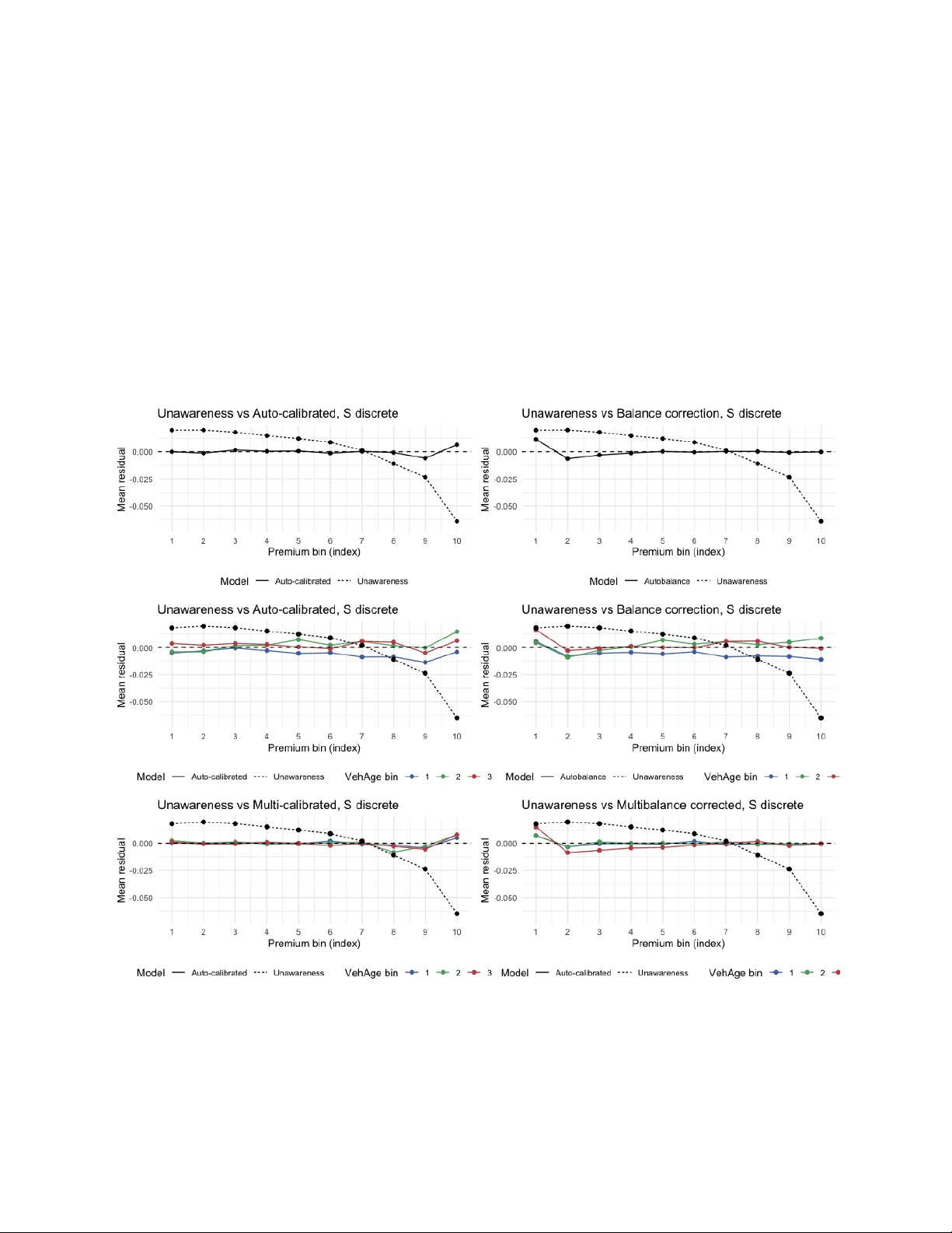
BALANCE AND F AIRNESS THR OUGH MUL TICALIBRA TION IN NONLIFE INSURANCE PRICING Mic hel Den uit Institute of Statistics, Biostatistics and Actuarial Science Louv ai n Institute of Data Analysis and Mo deling UCLouv ain Louv ain- la-Neuv e, Belgium Marie Mic haelides Sc ho ol of Mathematical and Computer Sciences Actuarial Mathematics and Statistics Heriot-W att Univ ersit y Edin burgh, United Kingdom Julien T rufin Departmen t of Mathematics Univ ersit´ e Libre de Bruxelles (ULB) Brussels, Belgium Marc h 18, 2026 Abstract Auto calibration is kno wn to b e an imp ortant requiremen t for insurance premiums since it guaran tees that premium income balances corresp onding claims, on a verage, not only at p ortfolio lev el but also inside eac h group pa ying similar premiums. Also, fairness has become a ma jor concern b ecause unfair treatment may exp ose insurers to la wsuits or reputational damage. T ranslating fairness in to conditional mean indep endence allows actuaries to com- bine auto calibration and fairness in to the multicalibration concept. This paper studies the prop erties of multicalibration in an insurance context and prop oses practical w ays to im- plemen t it, through lo cal regression or bias correction within groups including credibility adjustmen ts. A case study based on motor insurance data illustrates the relev ance of m ul- ticalibration in insurance pricing. Keyw ords: Insurance pricing, auto calibration, fairness, sufficiency , m ulticalibration. 1 In tro duction and motiv ation Financial equilibrium is an imp ortan t prop ert y in insurance pricing as it ensures that pre- miums matc h corresp onding claims, on av erage. This prop ert y must hold at p ortfolio level (global balance) but also within meaningful groups of p olicyholders. Numerical evidence suggests that candidate premiums pro duced b y mac hine learning to ols, like b oosted regres- sion trees or neural net works, can depart substan tially from observed claim totals. See, e.g., Den uit et al. (2019) and the references therein. Auto calibration has b een prop osed as a remedy by Denuit et al. (2021), Den uit and T rufin (2023, 2024), Lindholm et al. (2023), W ¨ uthric h (2023) and W ¨ uthrich and Ziegel (2024) since it ensures that the amoun ts col- lected from p olicyholders pa ying the same premium match the corresp onding claim totals, on a verage. Besides financial equilibrium, discrimination is another imp ortant issue in the priv ate insurance industry . W e refer the reader, e.g., to F rees and Huang (2023) and Charp en tier (2024) for a general o verview of the topic. The ban of gender-based discrimination within the Europ ean Union (EU) is emblematic in that resp ect. In 2011, the Europ ean Court of Justice concluded that any gender-based insurance discrimination must be prohibited. F rom Decem b er 21, 2012, all insurers op erating in the EU are required to offer unisex premiums and b enefits. In North-America, race is another example of protected feature in several states and pro vinces. The protected attributes listed in the EU Directiv es are particularly relev ant for insurers op erating in the EU. In addition to gender, this list includes some other features that are often used in insurance like age, health or disability status, for instance. As another example, F r¨ ohlic h and Williamson (2024) consider “ha ving migrant bac kground” as sensitiv e feature in their study of fair machine learning techniques. The EU directive banning the use of gender in insurance risk classification imp oses indi- vidual fairness. In general, this means that the amoun ts of premium c harged to policyholders differing only on the prohibited feature must b e equal. In this case, the sensitive feature is not included in the risk classification sc heme and commercial premiums do not depend on the sensitiv e feature in an explicit w ay . How ev er, indirect, or proxy discrimination may remain presen t when some rating factors included in the price list are correlated to the omitted sen- sitiv e feature. F or instance, motor insurance premiums often differ according to the p o wer of the v ehicle or the distance trav eled. If these features are correlated to gender, b ecause men tend to driv e more pow erful cars o ver longer distances for example, then insurance premiums still indirectly discriminate according to gender. EU guidelines precisely consider this case, as explained later on. This pap er considers the case of a sensitive feature not sub ject to individual fairness b y the la w. The insurer ma y th us let commercial premiums v ary according to the sensitiv e feature. T ypical examples include protected v ariables like health or disability status that are used by insurers or proxy v ariables to a forbidden rating factor. Because the use of these features may exp ose the insurer to complain ts from consumers organizations or formal in vestigation by the regulatory authorities, it is imp ortan t to b e able to prov e that the price list is fair with resp ect to the sensitive feature under scrutiny , in some sense to b e defined. There are sev eral approac hes to fairness in the insurance and in the machine learning liter- ature. Let us men tion actuarial fairness, individual fairness (or fairness through una w areness after Dw ork et al., 2012), counterfactual fairness (Kusner et al., 2017), and sev eral group- 1 fairness criteria (indep endence, separation, and sufficiency after Baro cas et al., 2019). In this pap er, w e follo w Baumann and Loi (2023) who adv o cate the relev ance of a weak v ersion of sufficiency in insurance pricing. This group-fairness notion imp oses conditional mean in- dep endence of the resp onse and the sensitiv e feature, giv en the premium. Being based on conditional mean indep endence, sufficiency is in tuitively appealing and nicely com bines with auto calibration, resulting in the concept of multicalibration in tro duced by Heb ert-Johnson et al. (2018). In w ords, a premium is m ulticalibrated with resp ect to a collection of groups partitioning the p ortfolio if it is auto calibrated within eac h group, in addition to b eing au- to calibrated o verall. The groups considered in this pap er are formed based on the sensitive feature. The reinforcement of sufficiency in to m ulticalibration is men tioned as an a ven ue for future research in Section 3.3 in Baumann and Loi (2023) while calibration conditional on gender and on salary has b een implemented by Fissler et al. (2022) in their application to w orkers’ comp ensation insurance. This pap er develops these ideas and bridges fairness to auto calibration. The remainder of this pap er is organized as follo ws. The insurance ratemaking prob- lem is formalized in Section 2. Section 3 recalls the auto calibration concept. Section 4 is dev oted to fairness notions. The group-fairness concept based on conditional mean indep en- dence considered in this pap er is in tro duced there. Section 5 unites auto calibration fairness through m ulticalibration while Section 6 explains how to implemen t m ulticalibration through m ultibalance correction. Numerical illustrations are given in Section 7. The final Section 8 summarizes the main con tribution of this pap er and discusses the results. 2 Nonlife insurance pricing The machine learning literature mainly considers binary outcomes and algorithmic decision- making systems. Typical examples include criminal risk assessment, hiring, college admis- sion, lending or so cial services interv ention, for instance, corresp onding to “y es-no” situ- ations. A binary resp onse is useful at underwriting stage in insurance where the insurer decides to co ver the risk or to refuse it. How ev er, claim-related resp onses (claim num b ers, claim severities, and claims totals) en ter the analysis when w e consider insurance pricing and these resp onses are not binary (integer, contin uous or mixed nature). In this pap er, w e consider a general claim-related resp onse Y ≥ 0. T o fix the ideas, it is useful to consider that Y corresp onds to the annual claim frequency for a p olicyholder in the p ortfolio. In accordance with credibility theory , we denote as M the true mean v alue of Y , suc h that E[ Y | M = µ ] = µ. The random v ariable M is assumed to hav e finite exp ectation. Notice that the last identit y can b e rewritten as E[ Y | M ] = M , almost surely . Throughout the pap er, ev ery equalit y b et ween random v ariables is assumed to hold with probabilit y 1, or almost surely . The true mean M remains unobserved and purely conceptual but is nevertheless useful to formalize the insurance ratemaking problem where M corresp onds to the pure premium that should b e charged by the insurer. This is b ecause individual departures Y − M cancel out in an y large insurance p ortfolio where a law of large n umbers applies. Charging M 2 corresp onds to actuarial fairness, which is practically imp ossible b ecause M cannot b e ob- serv ed. Contrary to algorithmic fairness problems, risk classification in insurance targets M whic h cannot b e observed at individual lev el. A t the collectiv e level, the distribution of M reflects the composition of the insured p opulation targeted by the insurance compan y under consideration. Since M is unkno wn, the insurance compan y can only use information recorded in its database ab out each p olicyholder. This corresp onds to the set of features X 1 , . . . , X p gath- ered in the random v ector X . Here, the information X is used as a substitute to M so that w e assume that Y and X are indep enden t given M . Actuarial pricing then aims to ev aluate the pure premium as accurately as p ossible, based on X . This means that the target is the conditional exp ectation µ ( X ) = E[ Y | X ] of the resp onse Y given the av ailable information X . Henceforth, µ ( X ) is referred to as the b est-estimate price after Lindholm et al. (2022). Notice that the conditional indep endence assumption allows us to write µ ( X ) = E  E[ Y | X , M ]   X  = E[ M | X ] so that µ ( X ) also approximates the individual premium M based on the information av ail- able to the insurance compan y . The unknown function x 7→ µ ( x ) = E[ Y | X = x ] is approximated b y a tec hnical pre- mium x 7→ π 0 ( x ). The tec hnical premium is the most accurate approximation to µ ( X ), for in ternal use, only . It allows the insurance company to compute p olicyholder v alue, for instance, by comparing the an ticipated cost π 0 ( X ) to the actual rev enues generated b y the con tract. These reven ues corresp ond to the commercial premium π ( X ) actually charged for co verage (excluding taxes, commissions and general exp enses). The premium structure π ( · ) is generally simplified compared to π 0 ( · ), dropping some features or using them at a less gran ular level. Henceforth, we assume that π 0 ( X ), π ( X ), and µ ( X ) are contin uous random v ariables admitting p ositiv e probability densit y functions ov er (0 , ∞ ). This eases exp osition and is generally the case when there is at least one con tinuous feature contained in the av ailable information X and the functions π 0 ( · ) and π ( · ) are con tinuously increasing functions of real scores built from X . Typically , a log-link is used and π 0 ( x ) = exp(score 0 ( x )) where score 0 ( x ) is obtained from b oosting, random forests or neural netw orks. Also, π ( x ) is the exp onential of an additiv e score pro duced b y a Generalized Additiv e Mo del for transparency and to comply with the multiplicativ e premium structure implemented in the ma jorit y of insurance commercial IT systems. Notice that we assume throughout the pap er that commercial premiums v ary according to rating factors related to risk, only , without non-risk based corrections (like price w alking, for instance). F or simplicity , we assume that the co v erage p erio d is 1 y ear. Exp osure can b e included in the analysis to account for shorter cov erage p erio ds, if needed, as is done in Section 7 for the numerical illustrations. F airness is meaningful only for the commercial premium π ( X ). T o figure out the situ- ation, it is useful to think ab out the example of gender within EU, which nev er enters the commercial premium since its use is prohibited but whic h generally impacts on the tec hnical premiums. The commercial premium can b e regarded as the decision made b y the insurance compan y ab out the policyholder while the tec hnical premium corresp onds to the prediction, as defined in Scan tam burlo et al. (2025). Since π 0 ( · ) is for in ternal use, only , there is no need 3 for it to b e fair. On the contrary , it must b e as accurate as p ossible so that the insurance compan y is able to counteract adv erse selection and to monitor premium transfers induced within the portfolio b y the application of the commercial premiums. Precisely , an y departure π ( X ) − π 0 ( X ) corresp onds to a transfer to (if p ositive) or from (if negativ e) another risk profile. The pap er concentrates on π ( · ) for whic h financial equilibrium and fairness b oth make sense. It is nev ertheless worth men tioning that the fairness notion studied in this pap er im- pro ves the p erformances of an y candidate premium. Hence, it is also meaningful for tec hnical premiums to impro ve accuracy as measured by any Bregman loss, including deviance. 3 Auto calibration In general, auto calibration ensures that the a v erage resp onse in a neighborho o d defined with the help of the auto calibrated predictor under consideration matches the predictor v alue. See, e.g., Kr ¨ uger and Ziegel (2021). Under auto calibration, the amoun ts collected from p olicyholders pa ying the same premium match the corresp onding claim totals, on a verage. Subsidizing transfers b etw een policyholders are th us av oided, helping to preven t adv erse selection effects. This concept is formally defined next, in the con text of insurance. Definition 3.1. The commercial premium π ( · ) is said to b e auto calibrated if E[ Y | π ( X ) = p ] = p for all premium amount p. (3.1) Auto calibration is an imp ortant prop ert y in insurance pricing b ecause it ensures that ev ery group of p olicyholders paying the same premium is on av erage self-financing. In other w ords, (3.1) guarantees that the premium paid by p olicyholders c harged the same amoun t of premium p exactly co vers the exp ected claims of that group. Notice that (3.1) can b e equiv alently rewritten as E[ Y − π ( X ) | π ( X ) = p ] = E[ µ ( X ) − π ( X ) | π ( X ) = p ] = 0 for all premium amoun t p. This sho ws that the net cash-flows Y − π ( X ) as well as the pricing errors µ ( X ) − π ( X ) cancel out within groups of p olicyholders pa ying the same amoun t of premium, on av erage. Auto calibration thus app ears to b e a very app ealing requiremen t for candidate premiums. F rom a conceptual p oin t of view, (3.1) can also b e written in terms of the true mean M as E[ M | π ( X )] = π ( X ) whic h ensures that the commercial premium also captures the premium that should b e c harged, on a verage. Notice that w e can equiv alently condition with resp ect to the score in (3.1) when π ( X ) is obtained by exp onen tiating an additive score. 4 F airness notion 4.1 Sensitiv e feature Assume now that there is a sensitiv e feature S recorded in the database. Its use is allow ed but requires particular atten tion b ecause it exposes the insurer to p ossible complaints ab out 4 unfair treatmen t. In this pap er, w e assume that S = X j 0 for some j 0 ∈ { 1 , 2 , . . . , p } to ease exp osition; see Remark 4.2 b elo w for a discussion. This means that the insurer actually uses S for premium calculation but wan ts to demonstrate that it is used in a fair and resp onsible w ay . T ypical examples for S include sensitiv e features like health or disabilit y status, or so cio-economic profile, for instance. In the situation where individual fairness is imp osed b y the law, lik e with gender in the EU for instance, S ma y corresp ond to a feature which is correlated to the prohibited one, as sho wn in the next example. Example 4.1. Considering the ban of gender-based discrimination in the EU, the individ- ual fairness imp osed by the law means that the premium π ( · ) m ust fulfill the constraint π ( x , man) = π ( x , w oman) = π ( x ) for all risk profiles x . In words, this means that a man and a w oman with the same rating factors x must pa y the same premium. If this condition is not fulfilled then direct discrimination results. This requirement is th us similar to the no- tions of “fairness through unaw areness” or “blindness”, except that the law partly prohibits the use of pro xies. According to Article 17 of the “Guidelines on the application of Council Directiv e 2004/113/EC to insurance, in the light of the judgmen t of the Court of Justice of the European Union in Case C-236/09 (T est-Ac hats)”, the use of true risk factors that migh t b e correlated with gender remains p ermitted. Examples are given to illustrate the extent of the prohibition. In a n utshell, the insurer is not allow ed to include in its price list a feature without impact on claims but correlated to gender. Hence, the use of proxy v ariables as substitutes for gender remains p ermitted, even if it generates indirect discrimination. Here, S would b e a rating factor X j 0 strongly correlated to gender while b eing a true risk factor if the insurance compan y wishes to demonstrate that it complies not only with the letter but also with the spirit of the an ti-discrimination law. R emark 4.2 . Even if the pap er concen trates on the case S = X j 0 for some j 0 ∈ { 1 , 2 , . . . , p } , the sensitiv e feature S migh t also result from a combination of several features in X , lik e disabilit y and area, for instance, to ensure equal access to insurance for disabled p eople whatev er their living area. A similar analysis can b e p erformed in these more complicated cases where S = ψ ( X ) for some giv en function ψ . Notice that S may ev en be another prediction or premium. F or instance, ψ ( X ) could b e the prediction of p olicyholder’s gender based on the rating factors X . R emark 4.3 . The case where S is not con tained in, or deduced from X is not relev ant for practice under the fairness notion considered in this pap er. Indeed, this situation would mean either that the use of S is prohibited b y the law or that the insurer refuses to let premiums dep end on S . If we except the case where Y and S are indep endent given π ( X ), an y fair premium (in the sense of multicalibration introduced b elo w) necessarily dep ends on S so that it conflicts with the ban imp osed b y the law or the commercial decision b y the insurer. 4.2 Sufficiency While individual fairness requires that individuals who only differ with resp ect to the pro- hibited feature must b e treated equally , group fairness is a global notion resulting from the comparison of groups defined by the sensitive feature S . Group fairness requires that b en- efits or harms resulting from the adoption of a pricing structure π ( · ) are distributed fairly 5 across these groups, where the fair distribution is defined from an appropriate group-fairness criterion. Classical group-fairness criteria include indep endence, separation and sufficiency . See, e.g., Baumann and Loi (2023) and Charp en tier (2024) for a discussion in the context of insurance. In general, there is no consensus ab out the fairness criterion and differen t con texts may call for different criteria. Moreo ver, fairness criteria are often incompatible so that one criterion must b e selected. In accordance with the analysis conducted b y Baumann and Loi (2023), sufficiency app ears to b e an appropriate fairness condition in the context of priv ate insurance. In its strict sense, sufficiency corresp onds to conditional indep endence of Y and S given π ( X ). This is a rather strong requiremen t that rules out demographic parit y whic h requires indep endence of π ( X ) and S . According to Charp entier (2024, Prop osition 9.3), if a candidate premium π ( · ) satisfies indep endence and sufficiency with resp ect to S then Y and S are indep enden t. Therefore, unless S do es not influence Y , no premium π ( · ) can sim ultaneously fulfill demographic parity and sufficiency . In this pap er, we consider the w eaker v ersion of sufficiency retained b y Baumann and Loi (2023), defined with the help of conditional mean indep endence of Y and S giv en π ( X ). The conditional mean indep endence concept is used in econometrics to decide whether additional features are needed in a regression mo del. It turns out that it also p ossesses an intuitiv e in terpretation in the context of insurance premium. This leads to the follo wing definition. Definition 4.4. A premium π ( · ) is said to be fair with respect to a sensitiv e feature S = X j 0 v alued in S if E[ Y | π ( X ) = p, S = s ] = E[ Y | π ( X ) = p, S = s ′ ] for all p and s, s ′ ∈ S . (4.1) The requirement (4.1) is intuitiv ely app ealing. It just means that the exp ected b enefits are equal across groups created by S provided the same amoun t of premium is paid. This argumen t ma y b e used by the insurer as a pro of that the use of S in premium calculation is resp onsible and protects p olicyholders’ righ ts b ecause the return from the insurance op- eration (measured by the amount Y paid b y the insurer) is the same, on av erage, as long as the premium is iden tical. If Y ∈ { 0 , 1 } then (4.1) corresp onds to the conditional indep endence of Y and S given π ( X ). How ev er, for more general resp onses lik e claim frequencies and severities, (4.1) is a w eaker requiremen t. Conditional mean indep endence can b e tested from data. The reader is referred to Lundb org (2022) for a survey and to Zhang et al. (2025) for recen t dev elopments on testing pro cedures. 5 Multicalibration 5.1 Definition Giv en that auto calibration is a central concept in insurance pricing, ro oted in financial equi- librium, it is th us natural to combine it with conditional mean indep endence (4.1) retained as group-fairness notion. It turns out that this corresp onds to the concept of multicalibra- tion prop osed in the machine learning literature b y Heb ert-Johnson et al. (2018). This is formally defined next. 6 Definition 5.1. The commercial premium π ( · ) is said to b e multica librated with respect to a sensitiv e feature S = X j 0 v alued in S if E[ Y | π ( X ) = p, S = s ] = E[ Y | π ( X ) = p, S = s ′ ] = p for all p and s, s ′ ∈ S . (5.1) Compared to (4.1), w e see that (5.1) not only imp oses the equalit y of conditional exp ec- tations, but also that they coincide with the premium amoun t p inv olved in the conditions. Notice that (5.1) can b e equiv alently rewritten as E[ Y − π ( X ) | π ( X ) = p, S = s ] = 0 for all p and s ∈ S . The net losses Y − π ( X ) th us av erage out in any group of p olicyholders pa ying the same amoun t of premium whatev er the v alue s of the sensitiv e feature S . This expresses the comp ensation of claims with premiums in these groups and recalls the balance equations at the heart of the metho d of marginal totals. Also, (5.1) can b e rewritten as E[ µ ( X ) − π ( X ) | π ( X ) = p, S = s ] = 0 for all p and s ∈ S . This shows that the pricing errors µ ( X ) − π ( X ) cancel out on av erage within groups of p olicyholders pa ying the same amount of premium and having the same v alue s of the sensitiv e feature S . Multicalibration th us app ears to b e a very app ealing requirement for commercial premiums. 5.2 Prop erties Let us first establish that m ulticalibration reinforces auto calibration. Prop ert y 5.2. (i) A ny multic alibr ate d pr emium π ( · ) with r esp e ct to S = X j 0 is also au- to c alibr ate d. (ii) If π ( · ) is auto c alibr ate d then c onditional me an indep endenc e (4.1) implies multic alibr a- tion with r esp e ct to S = X j 0 . Pr o of. F or an y multicalibrated premium, we hav e E[ Y | π ( X )] = E  E[ Y | π ( X ) , S ] | {z } = π ( X )   π ( X )  = π ( X ) so that it is also auto calibrated, as announced under item (i). Considering item (ii), notice that (4.1) together with auto calibration imply E[ Y | π ( X ) , S ] = E[ Y | π ( X )] = π ( X ) . This ends the pro of. All the prop erties deriv ed for autocalibrated premiums thus also hold for multicalibrated premiums. In particular, m ulticalibrated predictors nev er o v erfit. This has b een formalized for auto calibrated predictors with the help of the con v ex order. Recall from Den uit et al. 7 (2005, Section 3.4) that giv en t wo random v ariables Z and T , with finite exp ectations, T is said to b e smaller than Z in the conv ex order (denoted as T ⪯ cx Z ) if E[ g ( T )] ≤ E[ g ( Z )] for all conv ex functions g , (5.2) pro vided the exp ectations exist. In w ords, T ⪯ cx Z means that T is less disp ersed than Z while T and Z hav e the same exp ected v alue. In particular, V ar[ T ] ≤ V ar[ Z ]. According to Lemma 3.1 from W ¨ uthric h (2023), w e kno w that π ( X ) ⪯ cx µ ( X ) holds for an y auto calibrated π ( · ). Therefore, any multicalibrated premium π ( · ) with resp ect to S = X j 0 satisfies π ( X ) ⪯ cx µ ( X ) ⪯ cx Y . This shows that multicalibration prev ents ov erfitting, in the sense that an auto calibrated premium cannot b e more v ariable than µ ( X ) nor Y . W e know that µ ( X ) is auto calibrated as E[ Y | µ ( X )] = E  E[ Y | µ ( X ) , X ]   µ ( X )  = E  E[ Y | X ]   µ ( X )  = µ ( X ) . The next result sho ws that µ ( X ) is also multicalibrated with resp ect to S = X j for every j ∈ { 1 , . . . , p } . Prop ert y 5.3. The b est-estimate pric e µ ( X ) is multic alibr ate d with r esp e ct to any S = X j , j = 1 , 2 , . . . , p . Pr o of. It suffices to write E[ Y | µ ( X ) , S ] = E  E[ Y | µ ( X ) , S , X ]   µ ( X ) , S  = E  E[ Y | X ]   µ ( X ) , S  = µ ( X ) , whic h ends the pro of. Since pure premiums corresp ond to conditional exp ectations, they can thu s b e consis- ten tly estimated only if the exp ected loss is minim um for the mean resp onse. The class of Bregman loss functions is kno wn to b e strictly consistent for the (conditional) mean func- tional so that they are the only meaningful loss functions in the context of insurance pricing. F or a conv ex function ℓ ( · ), recall that the Bregman loss function L ( · , · ) is defined as L ( y , m ) = ℓ ( y ) − ℓ ( m ) − ℓ ′ ( m )( y − m ) (5.3) where ℓ ′ denotes the subgradien t of the conv ex function ℓ . A premium π 2 ( · ) outp erforms π 1 ( · ) for the Bregman loss function L in (5.3) if E[ L ( Y , b π 2 ( X ))] ≤ E[ L ( Y , b π 1 ( X ))]. Since m ulticalibrated predictors are also auto calibrated, we know from Theorem 3.1 in Kr ¨ uger and Ziegel (2021) that given t wo m ulticalibrated premiums π 1 ( · ) and π 2 ( · ), the inequality E[ L ( Y , π 2 ( X ))] ≤ E[ L ( Y , π 1 ( X ))] holds true for ev ery Bregman loss function L in (5.3) if, and only if, π 1 ( X ) ⪯ cx π 2 ( X ). This shows that the con vex order is the appropriate to ol to compare the relativ e p erformances of multicalibrated premiums. 8 6 Multibalance correction Balance correction has been prop osed as a practical w ay to restore autocalibration b y Den uit et al. (2021). Precisely , the balance-corrected v ersion π bc ( · ) of the candidate premiums π ( · ) is defined as π bc ( X ) = E[ Y | π ( X )] . (6.1) The new premium π bc ( · ) obtained from (6.1) is alwa ys auto calibrated as sho wn in Prop osition 3.3 in W ¨ uthric h (2023) without the monotonicity condition assumed in Den uit et al. (2021). The in tuition b ehind (6.1) is that π ( · ) is informativ e but not necessarily on the righ t scale, so that financial equilibrium defining auto calibration is violated. The conditional exp ectation (6.1) corrects the candidate premium by retaining the order induced by π ( · ) but av eraging insurance losses corresp onding to the same v alue of π ( X ). Inspired from balance correction (6.1) restoring auto calibration, let us introduce multi- balance correction restoring m ulticalibration. Definition 6.1. The m ultibalance-corrected version π mbc ( · ) of the premium π ( · ) with respect to S is defined as π mbc ( X ) = E[ Y | π ( X ) , S ] . (6.2) The next result shows that the premium π mbc ( · ) obtained b y m ultibalance correction (6.2) is alw ays multicalibrated with resp ect to S . Prop osition 6.2. The multib alanc e-c orr e cte d version π mbc ( · ) of the pr emium π ( · ) define d in (6.2) is multic alibr ate d with r esp e ct to S = X j 0 . Pr o of. The announced result follows from E[ Y | π mbc ( X ) , S ] = E  Y   E[ Y | π ( X ) , S ] , S  = E h E  Y   E[ Y | π ( X ) , S ] , S, π ( X )     E[ Y | π ( X ) , S ] , S i = E h E  Y   S, π ( X )     E[ Y | π ( X ) , S ] , S i = E  π mbc ( X )   π mbc ( X ) , S  = π mbc ( X ) , whic h ends the pro of. It turns out that multibalance correction impro ves the p erformance of the premium with resp ect to any Bregman loss function. This is precisely stated next. Prop osition 6.3. F or any pr emium π , we have E  L  Y , π ( X )  ≥ E  L  Y , π bc ( X )  ≥ E  L  Y , π mbc ( X )  ≥ E  L  Y , µ ( X )  for al l loss functions (5.3) . Pr o of. Since E[ Y | π ( X )] ⪯ cx E[ Y | π ( X ) , S ], we hav e π bc ( X ) ⪯ cx π mbc ( X ) ⪯ cx µ ( X ). The announced result then follo ws from Prop osition 4.5 in Den uit and T rufin (2024) and the equiv alence of Bregman dominance and conv ex order for auto calibrated predictors. 9 R emark 6.4 . The multibalance-corrected premium obtained from a candidate premium π ( · ) do es not necessarily coincide with the m ultibalance-corrected premium obtained from its balance-corrected v ersion π bc ( · ). Indeed, E[ Y | π bc ( X ) , S ] = E  E[ Y | π ( X ) , π bc ( X ) , S ]   π bc ( X ) , S  = E  E[ Y | π ( X ) , S ]   π bc ( X ) , S  = E  π mbc ( X )   π bc ( X ) , S  . Hence, the m ultibalance-corrected premium based on π bc ( · ) is obtained by av eraging the m ultibalance-corrected premium based on π ( · ) o v er the lev el sets of π bc ( · ), for eac h v alue of S . As a consequence, the tw o m ultibalance-corrected premiums ma y differ, since this a veraging can remov e information relev ant for predicting Y once S is given. They coincide if, and only if, conditioning with respect to π bc ( X ) retains all the predictiv e information carried b y π ( X ) for each v alue of S (that is, if and only if π ( X ) is measurable with resp ect to σ ( π bc ( X ) , S )). A simple sufficient condition for this to hold is that the mapping p 7→ E[ Y | π ( X ) = p ] b e one-to-one on the range of π ( X ), so that π ( X ) can b e reco vered from π bc ( X ). In particular, this condition is satisfied when the mapping p 7→ E[ Y | π ( X ) = p ] is strictly increasing, which means that π ( X ) induces the same ordering of risks as µ ( X ) = E[ Y | X ]. T o conclude this section, w e consider the case discussed in Remark 4.3, where the sensitiv e feature S is excluded from the set of admissible rating factors, either b ecause of regulation or of a commercial decision made b y the insurer. The next result sho ws how multibalance correction pro vides an illustration of the structural limitation highlighted in Remark 4.3. Prop osition 6.5. Assume that S is exclude d fr om the set of admissible r ating factors X . Then, for any admissible pr emium π ( · ) , the fol lowing statements hold. (i) The c orr esp onding pr emium π mbc ( · ) is multic alibr ate d with r esp e ct to S , in the sense that E[ Y | π mbc ( X , S ) , S ] = π mbc ( X , S ) . (ii) In gener al, π mbc ( · ) dep ends on S and ther efor e do es not define an admissible pr emium. (iii) The multib alanc e-c orr e cte d pr emium π mbc ( · ) do es not dep end on S if, and only if, E[ Y | π ( X ) , S ] = E[ Y | π ( X )] , that is, if, and only if, Y and S ar e c onditional ly me an-indep endent, given the pr emium π ( X ) . (iv) The multib alanc e c orr e ction c an b e written as π mbc ( X , S ) = E  E[ Y | X , S ]   π ( X ) , S  . In p articular, π mbc ( · ) c oincides with E[ Y | X , S ] if, and only if, E[ Y | X , S ] is me asur able with r esp e ct to σ ( π ( X ) , S ) . 10 Pr o of. By definition of the m ultibalance correction, π mbc ( X , S ) = E[ Y | π ( X ) , S ]. Therefore, E[ Y | π mbc ( X , S ) , S ] = E  E[ Y | π ( X ) , π mbc ( X , S ) , S ]   π mbc ( X , S ) , S  = E  E[ Y | π ( X ) , S ]   π mbc ( X , S ) , S  = E[ π mbc ( X , S ) | π mbc ( X , S ) , S ] = π mbc ( X , S ) . This pro ves the statement under item (i). Considering items (ii)-(iii), notice that π mbc ( X , S ) = E[ Y | π ( X ) , S ] generally dep ends on S . Hence, π mbc ( · ) is indep enden t of S if, and only if, E[ Y | π ( X ) , S ] = E[ Y | π ( X )] , whic h prov es the statements under items (ii)-(iii). Finally , E[ Y | π ( X ) , S ] = E  E[ Y | X , π ( X ) , S ]   π ( X ) , S  = E  E[ Y | X , S ]   π ( X ) , S  pro ves the statement under item (iv) and ends the pro of. Prop osition 6.5 provides an illustration of Remark 4.3. When S is excluded from the set of admissible rating factors X , m ulticalibration can only b e achiev ed in the exceptional case where Y and S are conditionally mean-indep endent, giv en the premium. Otherwise, enforcing multicalibration necessarily leads to premiums that dep end on S and are th us inadmissible. 7 Practical implemen tation of m ulticalibration This section prop oses practical w a ys to mak e a candidate premium π ( · ) m ulticalibrated with resp ect to a sensitiv e feature S included in X . The approac hes differ according to the format of S . 7.1 Categorical sensitive feature Assume that the sensitive feature S is categorical, with levels ℓ ∈ S . In principle, multi- calibration could b e implemen ted b y making π ( · ) auto calibrated separately in ev ery group S = ℓ , by replacing π ( · ) with its balance-corrected version π bc ( · ) for ev ery lev el of S . How- ev er, this simple approach is problematic if exp osures are limited for some groups, so that non-parametric smo othing do es not work. This section presents tw o empirical approaches to m ulticalibration. The first one im- plemen ts m ulticalibration through an explicit multibalance correction, while the second one enforces m ulticalibration directly through an iterativ e bias-correction pro cedure. Through- out this section, we consider a dataset of observ ations ( N i , X i , S i , w i ), i = 1 , . . . , n , where N i denotes the claim coun t, S i = X i,j 0 ∈ S the categorical sensitiv e feature and w i ≥ 0 kno wn w eights (t ypically exp osures). In practice, we use the observ ed claim frequency Y i = N i w i as resp onse v ariable, obtained by dividing the claim coun t b y the exp osure. 11 7.1.1 Direct empirical multibalance correction via group wise regression Multibalance correction amounts to restoring balance separately within each group defined b y the sensitive feature S . That is, instead of enforcing auto calibration globally , the balance condition is imp osed conditionally on S = ℓ , for every ℓ ∈ S . This principle can b e imple- men ted in sev eral wa ys, dep ending on ho w the conditional mean function E[ Y | π ( X ) , S = ℓ ] is estimated within each group. Examples include lo cal linear regression as in Ciatto et al. (2023) or isotonic regression as in W ¨ uthric h (2023). T o fix ideas, we describ e here an implemen tation based on isotonic regression. F or each lev el ℓ ∈ S , consider the conditional mean function m ℓ ( p ) = E  Y | π ( X ) = p, S = ℓ  , p > 0 . An empirical implemen tation of m ultibalance correction is obtained b y estimating m ℓ ( · ) non- parametrically within eac h group S = ℓ , under a monotonicit y constrain t in p . Sp ecifically , w e define b m ℓ as the solution of the w eighted isotonic regression problem b m ℓ ∈ argmin m non − decreasing X i : S i = ℓ w i  Y i − m ( π i )  2 , ℓ ∈ S , (7.1) restricting the search to non-decreasing conditional mean function, that is, such that p ≤ p ′ implies m ( p ) ≤ m ( p ′ ) on the range of { π i : S i = ℓ } . The resulting empirical multibalance- corrected premium is then obtained b y the plug-in rule b π mbc ( X i ) = b m S i  π ( X i )  , i = 1 , . . . , n, (7.2) where b m ℓ ( · ) is the solution to (7.1). This construction is the direct analogue of balance correction for auto calibration imple- men ted via isotonic regression by W ¨ uthrich (2023), except that the recalibration is performed separately within each lev el of the categorical sensitiv e feature S . By construction, the pre- mium b π mbc ( · ) in (7.2) is an empirical implemen tation of the multibalance-corrected premium π mbc ( X ) = E[ Y | π ( X ) , S ] , and therefore ac hieves multicalibration by enforcing balance conditionally on S . When some levels ℓ ∈ S carry limited exp osure, the fully nonparametric estimation in (7.1) ma y b e unstable, yielding step functions with high v ariance and p o or out-of-sample b eha vior. The next section therefore in tro duces a regularized pro cedure that relaxes the fully non-parametric group-wise approach. Rathe r than estimating conditional mean functions indep enden tly within each lev el of S , the pro cedure enforces balance on a finite collection of ( π , S )-cells and stabilizes lo cal corrections by b orro wing strength across groups through exp osure-driv en shrink age. 7.1.2 Regularized empirical enforcemen t of m ulticalibration via iterative bias correction W e now introduce a regularized empirical pro cedure that enforces multicalibration directly , without explicitly applying the multibalance correction. Starting from a baseline premium, 12 the pro cedure mo difies the premium iterativ ely so that, at the chosen level of discretization, a verage residuals v anish within each group defined b y the current premium level and the sensitiv e feature. Exp osure-driven shrink age is used to stabilize lo cal corrections when data are sparse. Binning and residual biases. Fix an in teger K ≥ 1. Starting from an initial premium π (0) ( · ) = π ( · ), consider at iteration j ≥ 0 a partition of the range of π ( j ) ( X ) into K disjoint in terv als { B ( j ) 1 , . . . , B ( j ) K } (for instance empirical quan tile bins). F or each observ ation i = 1 , . . . , n , define the residual R ( j ) i = Y i − π ( j ) ( X i ) . F or each bin k ∈ { 1 , . . . , K } and each level ℓ ∈ S , define the index set I ( j ) kℓ =  i : π ( j ) ( X i ) ∈ B ( j ) k , S i = ℓ  , together with the corresp onding exp osure w ( j ) kℓ = X i ∈ I ( j ) kℓ w i , w ( j ) k • = X ℓ ∈S w ( j ) kℓ . Whenev er w ( j ) kℓ > 0, define the cell-wise and p o oled bin-wise mean residuals as b b ( j ) kℓ = 1 w ( j ) kℓ X i ∈ I ( j ) kℓ w i R ( j ) i , b b ( j ) k = 1 w ( j ) k • X ℓ ∈S X i ∈ I ( j ) kℓ w i R ( j ) i . The quan tity b b ( j ) kℓ is the exp osure-w eighted sample analogue of E h Y − π ( j ) ( X )   π ( j ) ( X ) ∈ B ( j ) k , S = ℓ i . Exp osure-driv en shrink age. When w ( j ) kℓ is small, the estimate b b ( j ) kℓ is unstable. T o stabi- lize the correction, w e shrink b b ( j ) kℓ to ward the p o oled bin-lev el quan tity b b ( j ) k according to e b ( j ) kℓ = z ( j ) kℓ b b ( j ) kℓ +  1 − z ( j ) kℓ  b b ( j ) k , z ( j ) kℓ = w ( j ) kℓ w ( j ) kℓ + c , (7.3) where c > 0 is a tuning parameter controlling the amount of p o oling across groups. Up date step. Let η ∈ (0 , 1] b e a step size. F or each observ ation i suc h that π ( j ) ( X i ) ∈ B ( j ) k and S i = ℓ , up date π ( j +1) ( X i ) = π ( j ) ( X i ) + η e b ( j ) kℓ . (7.4) This up date adjusts the premium by an exp osure-regularized estimate of the residual bias in the corresp onding ( π , S )-cell. 13 Stopping criterion. Iterations are stopp ed when the remaining correction b ecomes neg- ligible. A con v enient criterion is to retain the solution such that max k,ℓ : w ( j ) kℓ > 0   η e b ( j ) kℓ   π ( j ) kℓ ≤ δ, where π ( j ) kℓ and e b ( j ) kℓ denote exp osure-weigh ted av erages of π ( j ) ( X i ) and e b ( j ) kℓ o ver i ∈ I ( j ) kℓ , and δ > 0 is a tolerance parameter selected by the actuary . In terpretation. At con vergence, the pro cedure yields a premium π ( J ) ( · ) such that, for eac h bin B ( J ) k and eac h lev el ℓ ∈ S , the exposure-weigh ted mean residual within the corresponding cell is close to zero. Equiv alen tly , at the resolution induced b y the binning sc heme, no systematic av erage deviation b et ween Y and π ( J ) ( X ) remains within groups defined b y ( π ( J ) ( X ) , S ). This prop ert y is the discrete coun terpart of the multicalibration requiremen t E[ Y | π ( J ) ( X ) = p, S = ℓ ] = p , p > 0, ℓ ∈ S , with exact conditioning replaced b y conditioning on bin mem- b ership. Because the bins are up dated along the iterations and are defined using the curren t premium π ( j ) ( · ), the resulting premium π ( J ) ( · ) should b e understo o d as enforcing multical- ibration through a fixed-p oin t prop erty , rather than as the result of a single application of the m ultibalance correction. In contrast, if the bins are fixed using the baseline premium π ( · ) and a single up date is per- formed, the pro cedure reduces to a discretized empirical approximation of the m ultibalance- corrected premium π mbc ( X ) = E[ Y | π ( X ) , S ], at the chosen binning resolution. On the role of credibility w eights. In the classical B ¨ uhlmann–Straub framework, cred- ibilit y arises from an explicit sto c hastic data-generating structure. A laten t parameter Θ go verns rep eated observ ations at individual risk lev el, leading to the w ell-kno wn v ariance decomp osition into pro cess v ariance and structural v ariance. In the presen t multicalibration setting, no suc h structural latent parameter is postulated. The pro cedure is entirely cross-sectional and algorithmic. F or a given premium bin k and group ℓ , the quan tity b kℓ = E[ Y − π ( X ) | π ( X ) ∈ B k , S = ℓ ] ma y b e viewed as a laten t systematic bias parameter attached to the cell ( k , ℓ ), but this parameter is induced b y the curren t premium rather than by an underlying sto chastic het- erogeneit y . The observ ations within each cell simply play the role of rep eated measurements used to estimate this conditional mean residual. The analogy with credibilit y theory is therefore algebraic rather than structural. As in the B ¨ uhlmann–Straub mo del, the empirical estimator b b kℓ is noisy when exp osure w kℓ is small. A v ariance decomp osition of the form V ar[ b b kℓ ] = E[ σ 2 kℓ ] w kℓ + V ar[ b kℓ ] 14 motiv ates shrinking the cell-sp ecific estimator to w ard the p o oled bin-lev el quantit y b b k , lead- ing to the w eight z kℓ = w kℓ w kℓ + c . The resulting correction e b kℓ = z kℓ b b kℓ + (1 − z kℓ ) b b k should therefore be in terpreted primarily as an exp osure-driven regularization device. It stabilizes local bias estimates in lo w-exp osure cells while allo wing more gran ular adjustmen ts where sufficien t data are av ailable. In con trast with classical credibility theory , ho w ever, we do not assume an explicit hier- arc hical mo del with a sto c hastic laten t parameter Θ. The credibility weigh t here pro vides a principled and actuarially interpretable shrink age mechanism, but the m ulticalibration pro cedure itself remains a p ost-processing algorithm rather than the consequence of a fully sp ecified probabilistic credibility mo del. 7.1.3 Numerical illustrations W e apply the prop osed m ulticalibration pro cedure to the data set used by Noll et al. (2018). This data set con tains a F renc h motor third-party liability (MTPL) insurance p ortfolio comprising of 677 991 entries, each corresp onding to a policy . Tw elve v ariables are observ ed for eac h of these p olicies, listed in T able 7.1. W e refer to Noll et al. (2018) for a detailed description of the complete data set. T able 7.1: Description of the v ariables in the freMTPL2freq dataset. V ariable Description IDpol P olicy num b er. ClaimNb Num b er of claims. Exposure T otal exp osure in yearly units. Area Area co de (A,B,C,D,E or F). Region Region of F rance where the p olicy is registered, categorical v ariable with 22 lev els. Density P opulation densit y (n umber of inhabitants p er square km) of the city where the p olicyholder lives. BonusMalus Bonus-malus level, ranging b et ween 50 and 230 (reference level: 100). DrivAge Age of the driv er of the vehicle, in years. VehAge Age of the v ehicle, in years. VehGas T yp e of fuel used for the vehicle (diesel or regular gas). VehPower P ow er of the car, categorical v ariable ranging from 4 to 15. VehBrand Brand of the car, categorical v ariable with 11 levels. 15 The outcome v ariable Y is the observed claim frequency , defined as Y = N w , where N = ClaimNb and w = Exposure measured in policy-years. F or the multicalibration analysis, w e consider a discrete sensitive attribute S d = bin VehAge , obtained by grouping VehAge into three bins of approximately equal size: (0 , 3], (3 , 9] and > 9. The rating v ariables are X = { Area , Region , Density , BonusMalus , DrivAge , VehAge , VehGas , VehBrand } , while bin VehAge is used solely for calibration. The data are randomly split in to training (60%), v alidation (20%), and test (20%) sets. Baseline premiums are obtained from a P oisson GAM with log-link and exp osure offset. Precisely , we assume that N i | X i ∼ Poisson  w i λ ( X i )  , with ln λ ( X i ) = β 0 + X m f m ( X i,m ) . The corresp onding frequency premium is then given by π ( X i ) = λ ( X i ) = E[ Y i | X i ] . Although π ( · ) is calibrated on av erage, it displa ys systematic residual bias across premium lev els and across vehicle-age groups. Starting from π ( · ), we consider fiv e premium constructions. The first is the unaw areness premium itself. The second corresp onds to auto calibration obtained as a limiting case of the iterativ e m ulticalibration procedure when the credibilit y parameter c is taken to b e v ery large. In that regime, z kℓ = w kℓ w kℓ + c ≈ 0 , so that only the bin-level bias enters the up date, enforcing auto calibration. As a non- iterativ e b enc hmark targeting the same ob jective, we also consider classical balance correc- tion π bc ( X ) = E[ Y | π 0 ( X )] based on w eighted isotonic regression, F ull multicalibration is obtained for finite c , com bining bin-lev el and cell-level biases through exp osure-driven shrink- age so as to enforce E[ Y − π ( X ) | bin , S ] ≈ 0. Finally , multibalance correction is defined b y π mbc ( X ) = E[ Y | π ( X ) , S ], estimated via w eighted isotonic regression within each v ehicle-age group. Throughout, w e use K = 10 premium bins, step size η = 0 . 2, and stopping threshold δ = 0 . 01. Residual bias is computed as exp osure-weigh ted av erages within each premium bin and v ehicle-age group. Figure 7.1 illustrates the residual structure. The baseline premiums exhibit a clear mono- tone distortion across premium bins, with pronounced under-pricing in the highest bins. 16 After auto calibration (iterative or isotonic), this global pattern disapp ears and the o ver- all residual curve b ecomes essentially flat. Ho wev er, significan t differences remain across v ehicle-age groups within the same premium bin, indicating p ersistent conditional bias with resp ect to S , as shown in the plot on the second row. Applying full m ulticalibration or m ultibalance correction remo ves these group-sp ecific distortions. In b oth cases, the colored curv es align closely around zero across all bins. Multicalibration ac hiev es this through iterative bias updates with exp osure-driv en shrink age, pro ducing smo oth residual profiles. Multibalance correction enforces conditional calibration directly via group-wise isotonic regression. Minor lo cal oscillations reflect the step-wise nature of the estimator and the absence of cross-group regularization. Overall, both metho ds successfully restore conditional balance while preserving premium-lev el calibration, with the iterativ e approach yielding slightly more regular patterns. Figure 7.1: Mean residual pricing bias across premium bins for discrete v ehicle-age groups. T op ro w: baseline vs. auto calibration. Middle ro w: auto calibration via iterative algorithm (left) and balance correction via isotonic regression (right). Bottom row: m ulticalibration (iterativ e) and multibalance correction (group-wise isotonic regression). 17 T able 7.2 rep orts out-of-sample p erformance on the test set using Poisson deviance and Gini co efficien t. The baseline mo del exhibits by far the highest deviance, confirming that miscalibration in the premium score materially affects predictive accuracy . Although the baseline GAM is estimated by maxim um lik eliho o d in the co v ariate space, it do es not guar- an tee that the induced premium satisfies auto calibration. Systematic distortions across premium levels therefore translate into lik eliho od losses when aggregated ov er the p ortfolio. Auto calibration yields a substan tial reduction in deviance relative to the baseline, show- ing that correcting premium-level distortions already impro ves adequacy . Introducing con- ditional calibration with resp ect to vehicle age further reduces deviance: the multicalibrated premium ac hieves the low est deviance ov erall, improving up on the auto calibrated sp ecifica- tion. In comparison, the non-iterative balance and m ultibalance corrections achiev e slightly higher deviance v alues. Overall, the iterativ e pro cedures (auto calibration and multicalibra- tion) outp erform their isotonic counterparts in terms of deviance. In terms of discriminatory p ow er, all calibrated mo dels substantially impro ve up on the baseline. The Gini co efficients of the calibrated mo dels are relativ ely close, with auto cali- bration and balance correction attaining the highest v alues. T able 7.2: Out-of-sample p erformance comparison on the test set. Mo del Deviance Gini Co efficien t Baseline 36 310.68 0.5783 Auto calibrated 33 882.79 0.7237 Balance correction 33 912.20 0.7221 Multicalibrated 33 779.73 0.6876 Multibalance correction 33 808.72 0.6938 7.2 Con tin uous sensitiv e feature W e now consider the case where the sensitive feature S is contin uous. In this setting, m ulticalibration enforces E[ Y | π ( X ) = p, S = s ] = p , for ( p, s ) in the supp ort of ( π ( X ) , S ). In analogy with the categorical case, we present tw o empirical approac hes. The first one implemen ts m ulticalibration through a direct estimation of the conditional mean surface in the joint ( π , S ) space. The second one enforces m ulticalibration through a regularized iterativ e bias-correction pro cedure. W e w ork with the same data structure as b efore. 7.2.1 Direct empirical multibalance correction via biv ariate lo cal GLM When the sensitiv e feature S is con tinuous, we estimate the conditional mean surface m ( p, s ) = E[ Y | π ( X ) = p, S = s ] , through a lo cal GLM in the joint ( π , S ) space. T o estimate m ( p, s ) at a given ( p, s ), we assign to eac h observ ation ( N i , π i , S i , w i ) a w eigh t ν i ( p, s ) = ν  π i − p h π , S i − s h S  , 18 where ν ( · , · ) is a symmetric weigh t function supp orted on a b ounded set and h π and h S > 0 are bandwidth parameters con trolling lo calit y in eac h direction. At ( p, s ), w e fit an in tercept- only GLM adapted to the nature of the resp onse, using exp osure w eights w i . Under the canonical link function g , w e obtain the lo cal likelihoo d equation n X i =1 ν i ( p, s ) w i Y i = n X i =1 ν i ( p, s ) w i µ ( p, s ) , whose solution yields b m ( p, s ) = P n i =1 ν i ( p, s ) w i Y i P n i =1 ν i ( p, s ) w i . The resp onse v ariable is again the observed claim frequency Y = N /w , and estimation is p erformed using an exp osure-w eighted lo cal GLM. A natural plug-in estimator replaces π ( X i ) with b m  π ( X i ) , S i  . While this estimator targets conditional balance with respect to ( π , S ), it do es not generally preserve marginal auto calibration with resp ect to π . T o restore marginal consistency , we therefore in tro duce a cen tering step. First, w e estimate the marginal conditional mean b m 0 ( p ) = E[ Y | π ( X ) = p ] using a one-dimensional lo cal GLM in the premium score. W e then define δ ( p, s ) = b m ( p, s ) − b m 0 ( p ) , and estimate its conditional exp ectation giv en p via a one-dimensional lo cal regression. De- noting this estimate b y b E[ δ ( p, S ) | π = p ], we construct the centered multibalance correction b π mbc ( X i ) = b m 0  π ( X i )  + δ  π ( X i ) , S i  − b E  δ  π ( X i ) , S  | π = π ( X i )  . This centering guarantees that the a verage correction at each premium level coincides with the marginal balance adjustment while redistributing residual bias across v alues of S . By construction, b π mbc ( X ) ≈ E[ Y | π ( X ) , S ], while preserving approximate autocalibration in the premium dimension. This pro cedure constitutes the con tinuous analogue of the group-wise multibalance cor- rection describ ed in Section 7.1.1. While it enforces conditional balance in a single smo othing step, its p erformance dep ends on the lo cal density of observ ations in the join t ( π , S ) space. In regions with limited exp osure, t wo-dimensional smo othing may b ecome unstable, which motiv ates the regulariaed iterative alternative in tro duced next. 7.2.2 Regularized empirical enforcemen t of m ulticalibration via iterative bias correction W e introduce a regularized empirical pro cedure that enforces multicalibration sequentially . Rather than estimating the full conditional mean surface in one step, w e iteratively re- mo ve residual bias in the joint ( π , S ) space, com bining one-dimensional and tw o-dimensional smo others with exp osure-driven shrink age to stabilize lo cal corrections. 19 Lo cal residual biases. Let π (0) ( X ) = π ( X ) denote the baseline premium. F or iterations j = 0 , 1 , 2 , . . . , J , define the residual R ( j ) i = Y i − π ( j ) ( X i ) . W e estimate tw o smo oth conditional mean functions at eac h iteration: b b ( j ) ( p ) = E  Y − π ( j ) ( X ) | π ( j ) ( X ) = p  , b b ( j ) ( p, s ) = E  Y − π ( j ) ( X ) | π ( j ) ( X ) = p, S = s  . The first term corresp onds to the marginal premium-level bias and plays the role of the bin- lev el bias in the discrete algorithm, thereb y enforcing auto calibration with resp ect to the premium. The second captures systematic deviations that remain conditional on b oth the premium level and the grouping v ariable. The one-dimensional and tw o-dimensional smo oth regressions are p erformed in the current premium space π ( j ) ( X ). Exp osure-driv en shrink age. T o stabilize local bias estimates in regions with limited data, we introduce credibility w eights in the join t ( π , S ) space. Prior to the iterativ e pro ce- dure, we use a k -nearest-neighbor estimator to approximate the lo cal densit y of observ ations around each p oin t ( p, s ) and conv ert it in to a lo cal effective exp osure w loc ( p, s ). W e define the credibilit y weigh t as z ( p, s ) = w loc ( p, s ) w loc ( p, s ) + c , where c > 0 is a tuning parameter controlling the amount of shrink age. In con trast with the categorical case, where credibility weigh ts dep end on iteration- sp ecific cell exp osures, the quan tity w loc ( p, s ) reflects intrinsic data a v ailability in the con- tin uous ( π , S ) space. W e therefore compute the weigh ts z ( p, s ) once and keep them fixed throughout the iterations. This choice ensures that shrink age captures structural sparsity of the data rather than fluctuations induced b y successive premium up dates and av oids feedbac k b etw een correction and regularization. W e define the credibility-w eighted conditional correction p oin twise as δ ( j ) ( p, s ) = z ( p, s )  b b ( j ) ( p, s ) − b b ( j ) ( p )  . As in Section 7.2.1, we apply a cen tering step to preserve auto calibration with resp ect to the premium lev el. W e therefore define e b ( j ) ( p, s ) = b b ( j ) ( p ) + δ ( j ) ( p, s ) − E  δ ( j ) ( p, S ) | π ( j ) ( X ) = p  . W e compute the centering term via a one-dimensional lo cal regression of δ ( j ) ( π ( j ) ( X ) , S ) on π ( j ) ( X ). e b ( j ) ( p, s ) = b b ( j ) ( p ) + δ ( j ) ( p, s ) − E  δ ( j ) ( p, S ) | π ( j ) ( X ) = p  . W e estimate the conditional exp ectation in the last term using the same one-dimensional lo cal smo othing step in the premium score. This guarantees that the correction in tegrates to b b ( j ) ( p ) at each premium lev el, thereb y main taining marginal auto calibration while redistributing residual bias across v alues of the contin uous grouping v ariable S . 20 Up date step. F or a step size η ∈ (0 , 1], we up date the premium additively as π ( j +1) ( X i ) = π ( j ) ( X i ) + η e b ( j )  π ( j ) ( X i ) , S i  . The step-size parameter η con trols the sp eed of adjustmen t, and w e c ho ose it to ensure stable con vergence of the algorithm. Stopping criterion. At initialization, we construct fixed grids for the premium and the grouping v ariable using quan tile-based partitions of π (0) ( X ) and S . W e use these grids exclusiv ely to ev aluate con vergence. F or eac h cell ( k , ℓ ) of this fixed grid, we compute the exp osure-w eighted a v erages π ( j ) kℓ and b ( j ) kℓ of the current premium and correction. W e stop the pro cedure when max k,ℓ    η b ( j ) kℓ    π ( j ) kℓ ≤ δ, for a user-sp ecified tolerance parameter δ > 0. In terpretation. Up on completion of the algorithm, w e obtain a premium π ( J ) ( · ) for whic h no systematic residual bias remains at the c hosen resolution in the joint ( π , S ) space. On the role of credibilit y weigh ts. As in the categorical case, we in terpret the link with classical B ¨ uhlmann–Straub credibilit y in an algebraic rather than structural sense. W e do not p ostulate any latent parameter Θ, and the pro cedure remains purely cross-sectional and algorithmic. In the con tinuous setting, we view b ( p, s ) = E[ Y − π ( X ) | π ( X ) = p, S = s ] as a latent systematic bias surface attached to the curren t premium. Observ ations lo cated near ( p, s ) pro vide rep eated information for estimating this conditional mean residual. When lo cal effective exp osure w loc ( p, s ) is small, these estimates b ecome unstable, which motiv ates shrink age tow ard the marginal bias. The credibility weigh t z ( p, s ) = w loc ( p,s ) w loc ( p,s )+ c therefore acts as an exp osure-driv en regular- ization device, reducing v ariance in sparse regions while allowing more granular adjustmen ts where sufficien t data are av ailable. W e thus use credibility as a stabilization mechanism rather than as the consequence of a hierarchical sto c hastic mo del, and the m ulticalibration pro cedure remains a p ost-pro cessing algorithm enforcing conditional balance. 7.2.3 Numerical illustrations W e no w illustrate the con tin uous m ulticalibration pro cedures using the same MTPL fre- quency dataset and data split as in Section 7.1.3. Here, we consider vehicle age as a con tin- uous grouping v ariable and set S = VehAge . 21 V ehicle age is not used as a rating v ariable but only as a calibration dimension. W e obtain baseline premiums π ( · ) from the same P oisson GAM with log-link and exp osure offset de- scrib ed previously . These premiums exhibit systematic residual distortions across premium lev els and conditional on vehicle age. Starting from π ( · ), we consider fiv e premium constructions. The first is the unaw areness premium itself. The second corresp onds to auto calibration obtained as a limiting case of the iterative algorithm when the credibilit y parameter c is large, enforcing auto calibration through one-dimensional lo cal regression in the premium score. As a direct non-iterative b enc hmark targeting the same ob jectiv e, w e also consider balance correction defined by π bc ( X ) = E[ Y | π ( X )] , estimated via a one-dimensional lo cal GLM. W e then compare tw o approaches enforcing conditional balance with resp ect to the con- tin uous v ariable S = VehAge . W e obtain full m ulticalibration through the iterativ e procedure of Section 7.2.2. A t each iteration, we estimate the marginal bias b b ( j ) ( p ) and the joint bias surface b b ( j ) ( p, s ) via lo cal GLMs in the current premium space, apply exposure-driven shrink- age, and cen tre the correction as describ ed in Section 7.2.1. The lo cal GLMs are estimated using the locfit function in R with neighborho o d parameter α = 0 . 5, representing the near- est neighbor fraction. W e use lo cal linear fits, step size η = 0 . 2, and stopping threshold δ = 0 . 01. As a direct non-iterative alternative, we implement m ultibalance correction via the cen- tered biv ariate lo cal GLM of Section 7.2.1. Specifically , we estimate the conditional mean surface m ( p, s ) = E[ Y | π ( X ) = p, S = s ] using a t wo-dimensional lo cal P oisson regression in the join t ( π , S ) space with the same smo othing parameters. W e then apply the centering step to preserv e marginal auto calibration. W e ev aluate residual bias on the v alidation set using ten premium bins constructed from π ( · ) and for eac h v alue of VehAge . F or visual clarity , these curves are summarised b y a shaded env elop e corresp onding to the minimum and maximum residual bias across vehicle ages within eac h premium bin. Figure 7.2 displays the residual structure. The baseline premiums show a clear monotone distortion across premium bins, with substan tial under- pricing in the highest bins. After auto calibration (iterativ e or direct balance correction), the global residual curv e b ecomes essen tially flat, confirming that b oth approac hes enforce auto calibration, as shown on the top panel. Ho wev er, disp ersion across v ehicle age remains visible within each premium bin, indicating p ersisten t conditional bias with resp ect to S , as illustrated by the wider shaded areas in the middle panel of Figure 7.2 for b oth approaches. Applying full multicalibration or m ultibalance correction substantially reduces this dis- p ersion. The shaded regions in the b ottom row narrow considerably relative to auto cali- bration, demonstrating that b oth metho ds effectively remov e conditional distortions along the con tin uous v ehicle-age dimension. The iterativ e m ulticalibration pro cedure yields the smo othest residual patterns, reflecting the stabilizing effect of shrink age and rep eated bias up dates. The direct m ultibalance correction ac hiev es comparable alignmen t in a single step, with minor lo cal v ariations attributable to finite-sample smo othing in t w o dimensions. T able 7.3 rep orts out-of-sample p erformance on the test set using Poisson deviance and Gini co efficien t. The pattern is again consisten t with the categorical case discussed in Sec- 22 Figure 7.2: Mean residual pricing bias across premium bins for contin uous vehicle-age. T op ro w: baseline vs. auto calibration. Middle row: auto calibration via iterative algorithm (left) and balance correction via isotonic regression (right). Bottom ro w: m ulticalibration (itera- tiv e) and multibalance correction (groupwise isotonic regression). tion 7.1.3. The baseline model exhibits the highest deviance, reflecting score-lev el miscalibra- tion. Auto calibration substantially reduces deviance, confirming that correcting premium- lev el distortions improv es mo del adequacy . In tro ducing conditional calibration with resp ect to con tinuous vehicle age yields further impro vemen ts. The m ulticalibrated premium ac hiev es the lo w est deviance o v erall, improving up on the auto calibrated sp ecification. The non-iterative balance and m ultibalance correc- tions attain v ery similar but sligh tly higher deviance v alues. Overall, the iterative pro cedures (auto calibration and multicalibration) pro vide the b est adequacy p erformance in the con tin- uous setting. In terms of discriminatory p ow er, all calibrated mo dels mark edly improv e up on the base- line. The Gini co efficients of the calibrated sp ecifications are relatively close. Multibalance correction attains the highest Gini v alue, follow ed closely b y balance correction and auto cal- 23 ibration, while m ulticalibration yields a slightly low er v alue. T able 7.3: Out-of-sample p erformance comparison on the test set. Mo del Deviance Gini Co efficien t Baseline 36 310.68 0.5783 Auto calibrated 33 793.14 0.6941 Balance correction 33 799.32 0.6973 Multicalibrated 33 781.86 0.6904 Multibalance correction 33 814.61 0.7023 8 Discussion This pap er implemented multicalibration for insurance premiums. This notion is particularly app ealing b ecause it ensures financial equilibrium and guaran tees that the exp ected return of the insurance operation is iden tical across groups defined on the basis of the sensitiv e feature. Sev eral metho ds for implemen ting multicalibration ha ve b een prop osed and illustrated on a motor insurance p ortfolio. In terestingly , m ulticalibration improv es the p erformances of the candidate premium whereas imp osing fairness generally deteriorates accuracy . Ac kno wledgemen ts The first Author gratefully ackno wledges funding from the FW O and F.R.S.-FNRS under the Excellence of Science (EOS) programme, pro ject AST eRISK (40007517). The third Author gratefully ackno wledges the supp ort received from the Research Chair ACTIONS under the aegis of the Risk F oundation, an initiative by BNP P aribas Cardif and the F renc h Institute of Actuaries. References - Baro cas, S., Hardt, M., Nara yanan, A. (2019). F airness and Machine Learning. fairml- b o ok.org. - Baumann, J., Loi, M. (2023). F airness and risk: An ethical argument for a group fairness definition insurers can use. Philosoph y & T echnology 36, article # 45. - Charp en tier, A. (2024). Insurance, Biases, Discrimination and F airness. Springer. - Ciatto, N., V erelst, H., T rufin, J., Den uit, M. (2023). Do es auto calibration improv e go o dness of lift? Europ ean Actuarial Journal 13, 479-486. - Den uit, M., Charp en tier, A., T rufin, J. (2021). Auto calibration and Tweedie-dominance for insurance pricing with machine learning. Insurance: Mathematics and Economics 101, 485-497. 24 - Den uit, M., Dhaene, J., Go o v aerts, M.J., Kaas, R. (2005). Actuarial Theory for De- p enden t Risks: Measures, Orders and Mo dels. Wiley , New Y ork. - Den uit, M., Szna jder, D., T rufin, J. (2019). Model selection based on Lorenz and concen tration curves, Gini indices and conv ex order. Insurance: Mathematics and Economics 89, 128-139. - Den uit, M., T rufin, J. (2023). Mo del selection with P earson’s correlation, concen tration and Lorenz curv es under auto calibration. Europ ean Actuarial Journal 13, 871-878. - Den uit, M., T rufin, J. (2024). Conv ex and Lorenz orders under balance correction in nonlife insurance pricing: Review and new developmen ts. Insurance: Mathematics and Economics 118, 123-128. - Dw ork, C., Hardt, M., Pitassi, T., Reingold, O., Zemel, R. (2012). F airness through a wareness. Pro ceedings Innov ations in Theoretical Computer Science Conference (ITCS 2012), pp. 214–226. - Fissler, T., Loren tzen, C., Ma y er, M. (2022). Model comparison and calibration as- sessmen t: User guide for consistent scoring functions in mac hine learning and actuarial practice. arXiv preprin t - F rees E. W., Huang F. (2023). The discriminating (pricing) actuary . North American Actuarial Journal 27, 2-24. - F r¨ ohlic h, C., Williamson, R.C. (2024). Insights from insurance for fair mac hine learn- ing. Pro ceedings of the 2024 A CM Conference on F airness, Accoun tability , and T rans- parency , pp. 407-421. - Heb ert-Johnson, U., Kim, M., Reingold, O., Roth blum, G. (2018). Multicalibration: Calibration for t he (computationally-iden tifiable) masses. Pro ceedings of In ternational Conference on Mac hine Learning, pp. 1939-1948. - Kr ¨ uger, F., Ziegel, J.F. (2021). Generic conditions for forecast dominance. Journal of Business & Economic Statistics 39, 972-983. - Kusner, M. J., Loftus, J., Russell, C., Silv a, R. (2017). Coun terfactual F airness. In Guy on, I., Luxburg, U. V., Bengio, S., W allach, H., F ergus, R., Vish wanathan, S., Garnett, R., (Eds.), Adv ances in Neural Information Pro cessing Systems, vol. 30. - Lindholm, M., Lindsk og, F., Palmquist, J. (2023). Lo cal bias adjustment, duration- w eighted probabilities, and automatic construction of tariff cells. Scandina vian Actu- arial Journal 2023, 946-973. - Lindholm, M., Richman, R., Tsanak as A., W¨ uthric h, M.V. (2022). Discrimination-free insurance pricing. Astin Bulletin 52, 55-89. - Lundb org, A. R. (2022). Mo dern methods for v ariable significance testing. PhD thesis, Ap ollo - Universit y of Cambridge Rep ository . 25 - Noll, A., Salzmann, R., W ¨ uthric h, M. (2018). Case study: F rench motor third-part y liabilit y claims. Av ailable at SSRN h ttps://ssrn.com/abstract=3164764. - Scan tamburlo, T., Baumann, J., Heitz, C. (2025). On prediction-mo delers and decision- mak ers: Why fairness requires more than a fair prediction mo del. AI & So ciety 40, 353-369. - W ¨ uthric h, M. V. (2023). Mo del selection with Gini indices under auto-calibration. Europ ean Actuarial Journal 13, 469-477. - W ¨ uthric h, M. V., Ziegel, J. (2024). Isotonic recalibration under a low signal-to-noise ratio. Scandina vian Actuarial Journal 2024(3), 279-299 - Zhang, Y., Huang, L., Y ang, Y., Shao, X. (2025). T esting conditional mean indep en- dence using generativ e neural netw orks. arXiv preprint 26