Safe Distributionally Robust Feature Selection under Covariate Shift

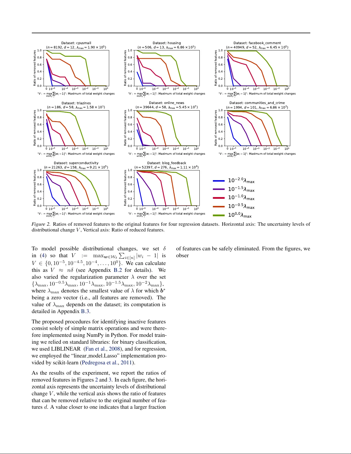
Safe Distrib utionally Rob ust F eatur e Selection under Cov ariate Shift Hiroyuki Hanada 1 Satoshi Akahane 1 Noriaki Hashimoto 2 Shion T akeno 1 Ichiro T ak euchi 1 2 Abstract In practical machine learning, the en vironments encountered during the model development and deployment phases often dif fer , especially when a model is used by many users in div erse set- tings. Learning models that maintain reliable performance across plausible deployment envi- ronments is kno wn as distrib utionally r obust (DR) learning . In this work, we study the problem of distributionally r obust featur e selection (DRFS) , with a particular focus on sparse sensing applica- tions motiv ated by industrial needs. In practical multi-sensor systems, a shared subset of sensors is typically selected prior to deployment based on performance ev aluations using many a v ailable sensors. At deployment, indi vidual users may fur- ther adapt or fine-tune models to their specific en vironments. When deployment en vironments differ from those anticipated during de velopment, this strategy can result in systems lacking sen- sors required for optimal performance. T o ad- dress this issue, we propose safe-DRFS , a nov el approach that extends safe screening from con- ventional sparse modeling settings to a DR setting under cov ariate shift. Our method identifies a fea- ture subset that encompasses all subsets that may become optimal across a specified range of input distribution shifts, with finite-sample theoretical guarantees of no false feature elimination. 1. Introduction In practical machine learning, model de v elopment and de- ployment are distinct phases, and uncertainty often arises in the deployment phase due to variations in operating en viron- ments. Distributionally r obust (DR) learning ( Mohajerin Es- fahani & Kuhn , 2018 ) has therefore attracted significant attention as a frame work for handling such uncertainty . In 1 Graduate School of Engineering, Nagoya Uni versity , Nagoya, Japan 2 Center for Advanced Intelligence Project, RIKEN, T okyo, Japan. Correspondence to: Hiroyuki Hanada < hanada.hiroyuki.i9@f.mail.nagoya-u.ac.jp > , Ichiro T akeuchi < takeuchi.ichiro.n6@f.mail.nagoya-u.ac.jp > . Pr eprint. Mar ch 18, 2026. its standard formulation, DR learning assumes that a model is fixed in the development phase and deployed without modification, with the goal of guaranteeing performance under the worst-case distribution within a prescribed uncer - tainty set. More recently , advanced DR learning settings hav e been explored in which the dev elopment phase de- termines a model backbone—such as a representation or structure—while allowing users to fine-tune or retrain mod- els in their deployment en vironments. In this case, the goal is to construct a rob ust foundation that ensures satisfactory performance e ven under worst-case deployment scenarios accounting for such adaptation. In this work, we study such an advanced DR learning setting that we term DR featur e selection (DRFS) . In the dev elop- ment phase, a system de veloper selects a subset of sensors (features) from a large pool of candidates, which are then physically equipped in a multi-sensor system and fixed at release. In the deployment phase, the released system is used by many individual users operating in dif ferent en vi- ronments, each of whom fine-tunes or retrains a model by selecting useful sensors from the fixed subset. When deploy- ment en vironments are uncertain and v ary across users, the sensor subset must therefore be constructed in a DR man- ner . This problem is motiv ated by industrial needs, where dev elopers must equip systems with all sensors that may be required under uncertain usage conditions while eliminat- ing unnecessary ones to reduce hardware cost and system complexity . As a specific instance of the DRFS problem, we consider sparse feature selection for regression and classification models under deployment environments subject to covari- ate shift ( Shimodaira , 2000 ). Specifically , users operate in en vironments where the input distribution deviates from that observed during de velopment. In each deployment environ- ment, users construct sparse models by selecting features from the fixed sensor set equipped in the system. The k ey challenge for the system de veloper is therefore to determine, during the development phase, a sensor subset that can cov er all features that may be selected across a range of plausible deployment en vironments. Figure 1 illustrates the problem setting considered in this work. Since the system dev eloper does not know in advance the en vironments in which the system will be deployed, sen- 1 Safe Distributionally Robust Featur e Selection under Covariate Shift M a ny A v a ila bl e S e ns o r s ( F e a t ur e s ) D ev el o p m en t P h a s e D e pl o y m e nt P ha s e ( F ix e d) M ult i - S en s o r S y s tem sen so r 1 sen so r 3 sen so r 4 sen so r 6 S y st em D ev el o p er D is t r ibut i o na l ly R o bus t F e a t ur e S e le ct io n ( D R F S ) sen so r 1 sen so r 3 sen so r 4 U ser 1 S pa r s e M o de ling sen so r 4 sen so r 6 S pa r s e M o de ling U ser 2 sen so r 3 sen so r 4 sen so r 6 S pa r s e M o de ling U ser 3 sen so r 1 sen so r 2 sen so r 3 sen so r 4 sen so r 5 sen so r 6 sen so r 7 F igur e 1. This figure illustrates the sparse sensing problem studied in this w ork, which consists of two phases: a de v elopment phase (top) and a deployment phase (bottom). In the de velopment phase, a system de veloper selects a subset of sensors from a large pool of candidates and designs a system equipped with these sensors, after which the sensor set is fix ed. In the deployment phase, the system is used by many end users operating in diverse en vironments with uncertainty , modeled as cov ariate shift, where the input distribution varies across users within a specified range. Each user adapts or fine-tunes a sparse model, such as a regression or classification model, using only the sensors av ailable in the system. Under co variate shift, the optimal support of sparse models may dif fer across users, leading to different sensor requirements. The key challenge for the dev eloper is therefore to select, during development, all sensors that may be required under plausible deployment en vironments while safely eliminating sensors that will ne ver be used. sors must be selected by accounting for worst-case cov ari- ate shifts within a prescribed range. Our ke y idea is to bring concepts originally dev eloped in the context of safe scr eening ( El Ghaoui et al. , 2012 ) into this DR learning setting. Safe screening was originally de v eloped to acceler- ate sparse optimization by identifying surely unnecessary features in the sense that their prediction coef ficients are zero (called inactive ) and eliminating them without affect- ing optimality . W e e xtend these screening criteria to certify feature rele v ance across en vironment-dependent covariate shifts. This extension enables the identification of sensors required under any plausible deployment en vironment and provides a complete finite-sample theoretical guarantee that no necessary features are e ver discarded; we thus refer to the proposed approach as safe-DRFS . Related W orks Distributionally Robust (DR) lear ning In the classical DR learning setup, a model is trained once in the devel- opment phase and deplo yed without further modification. The goal is to optimize the worst-case expected loss ov er an uncertainty set of test distributions, guaranteeing reli- able performance under the most adverse shift within the prescribed set ( Namkoong & Duchi , 2016 ; Shafieezadeh- Abadeh et al. , 2015 ; Mohajerin Esfahani & Kuhn , 2018 ; Namkoong & Duchi , 2017 ; Sinha et al. , 2018 ). While these formulations typically consider general forms of distrib u- tional uncertainty , including shifts in both input and output distributions, a prominent line of work focuses specifically on uncertainty in the input distribution, commonly modeled as cov ariate shift ( Shimodaira , 2000 ; Sugiyama et al. , 2007 ; K ouw & Loog , 2019 ). More recently , an advanced DR learning setting has emerged that assumes a two-stage workflow , where a dev eloper learns a robust base during de velopment and users adapt it at de- ployment via fine-tuning or test-time updates. This perspec- tiv e connects DR learning to test-time adaptation, personal- ization, and meta-learning, and has been explored in recent work allo wing deployment-time adaptation under distribu- tion shift ( W ang et al. , 2021 ; Sun et al. , 2020 ; Zhou et al. , 2021 ). A closely related recent work is ( Swaroop et al. , 2025 ), which studies feature selection under distrib ution shift. The y propose a DR objective function and tractable solution meth- ods based on continuous relaxations and heuristic optimiza- tion, b ut do not pro vide exact guarantees for the original robust problem. In contrast, our approach focuses on safe 2 Safe Distributionally Robust Featur e Selection under Covariate Shift certification by deriving explicit, computable worst-case bounds that enable feature elimination with finite-sample guarantees. Safe screening Safe screening techniques are designed to accelerate sparse learning by identifying features that are guaranteed to be inactiv e in the optimal solution and can therefore be safely removed without affecting optimality . The first such rule was proposed by El Ghaoui et al. ( 2012 ), followed by numerous extensions based on different opti- mality bounds ( W ang et al. , 2013 ; Liu et al. , 2014 ; W ang et al. , 2014 ; Xiang et al. , 2011 ). Among them, duality gap (DG)-based screening rules are particularly attracti ve due to their generality and ease of computation ( Fercoq et al. , 2015 ; Ndiaye et al. , 2015 ; 2017 ). Beyond standard sparse feature selection, the safe screen- ing principles have been extended and applied to a vari- ety of problems, including sample screening ( Ogaw a et al. , 2013 ; Shibagaki et al. , 2016 ), pattern and rule mining ( Nak- agaw a et al. , 2016 ; Kato et al. , 2023 ), model selection ( Oku- mura et al. , 2015 ; Hanada et al. , 2018 ), and finite-sample error bound computation ( Shibagaki et al. , 2015 ; Ndiaye & T akeuchi , 2019 ). Howe ver , to the best of our knowledge, safe screening principles ha ve not pre viously been applied to DR learning. Main Contributions This paper makes three main contributions. First, we formu- late, for the first time, a DR feature selection problem that explicitly accounts for deployment-time adaptation based on the safeness, that is, eliminating features that are assured not to af fect the prediction model in the deployment phase. Second, to achiev e this, we ne wly extended the methodol- ogy of safe screening — originally developed for acceler- ating sparse optimization — to be applied to DR learning, and demonstrate their effecti v eness for robust feature selec- tion. Finally , we deri ve computable w orst-case bounds that enable DR feature selection with finite-sample theoretical guarantees of no false feature elimination, and v alidate our theoretical results through empirical ev aluations. 2. Problem Setup W e consider a two-phase setting in multi-sensor systems. In the dev elopment phase, a system dev eloper selects a subset of sensors to be physically equipped in the system, which defines the features a v ailable for subsequent modeling. In the deployment phase, end users operate the fixed system in their o wn en vironments and adapt sparse models using the av ailable sensors. Since deployment en vironments may v ary across users, the system must include all sensors that could be required under plausible input distrib ution shifts. Our goal is therefore to select, during dev elopment, a feature subset that remains suf ficient across a specified range of deployment en vironments. Development phase During the de velopment phase, we are gi ven a dataset denoted by { ( x i , y i ) } i ∈ [ n ] , where x i ∈ X ⊆ R d is a d -dimensional feature vector defined in a domain X and y i ∈ Y is the corresponding response v ari- able. W e consider both regression and binary classification problems. In the regression setting, the response space sat- isfies Y ⊆ R , whereas in the binary classification setting, Y = {− 1 , 1 } . Here, the notation [ n ] = { 1 , 2 , . . . , n } de- notes the set of natural numbers from 1 to n . W e consider a linear model of the form f ( x i ; b , b 0 ) = x ⊤ i b + b 0 , i ∈ [ n ] , where b ∈ R d is a vector of feature coef ficients and b 0 ∈ R is the intercept term. Throughout the paper, we use the no- tation β := ( b , b 0 ) to express the feature coef ficient vector and the intercept term collectiv ely 1 . T o induce sparsity in the model, we employ L 1 -regularized estimation. Specifically , for both regression and binary classification problems, we consider empirical risk mini- mization (ERM) with an L 1 regularization term, gi v en by β ∗ := ( b ∗ , b ∗ 0 ) = argmin b ∈ R d , b 0 ∈ R X i ∈ [ n ] ℓ  y i , x ⊤ i b + b 0  + λ ∥ b ∥ 1 , (1) where ℓ ( · , · ) denotes a loss function and λ > 0 is a regu- larization parameter controlling the sparsity of the solution. In the regression setting, ℓ corresponds to a regression loss such as the squared loss ℓ ( y i , t ) := ( t − y i ) 2 , while in the binary classification setting, ℓ represents a classification loss such as the logistic loss ℓ ( y i , t ) := log(1 + e − y t ) . Due to the ef fect of sparse regularization, the optimal coefficient vector b ∗ is sparse. W e denote by S ( β ∗ ) ⊆ [ d ] the set of indices corresponding to the nonzero feature coefficients. Deployment phase In the deployment phase, we consider a setting in which the input distribution induced by each user’ s operating en vironment differs from that of the de- velopment phase within a certain range. Learning under such distributional discrepancies between de velopment and deployment en vironments is commonly referred to as co- variate shift . Under covariate shift, it is typically assumed that the conditional distribution of the response given the input remains unchanged, while the marginal input distri- bution v aries across en vironments. A standard approach to 1 In what follows, we use the notation β to collectiv ely represent a feature coef ficient vector and an intercept term; for example, expressions such as β ∗ or ˆ β correspond to the pairs ( b ∗ , b ∗ 0 ) and ( ˆ b , ˆ b 0 ) , respectiv ely . 3 Safe Distributionally Robust Featur e Selection under Covariate Shift addressing cov ariate shift is to formulate the learning prob- lem as a weighted ERM problem. Specifically , let P dev ( x ) and P dep ( x ) denote the input distributions in the develop- ment and deployment en vironments, respecti v ely . For each training instance ( x i , y i ) , we define a weight w i = P dep ( x i ) P dev ( x i ) , i ∈ [ n ] . (2) Assuming that the same dataset { ( x i , y i ) } i ∈ [ n ] is av ailable in the deployment phase, the weighted ERM problem is formulated using these weights as β ∗ ( w ) :=  b ∗ ( w ) , b ∗ ( w ) 0  (3) = argmin b ∈ R d ,b 0 ∈ R X i ∈ [ n ] w i ℓ  y i , x ⊤ i b + b 0  + λ ∥ b ∥ 1 | {z } =: P ( w ) ( β ) , where w = ( w 1 , . . . , w n ) ⊤ . Under the assumption of the cov ariate shift, the model trained with these weights is known to achie ve consistency ( Shimodaira , 2000 ; Sugiyama et al. , 2007 ). The sparse solution obtained by the weighted ERM in ( 3 ) has a set of nonzero coefficients S ( β ∗ ( w ) ) that does not necessarily coincide with S ( β ∗ ) . DR feature subset W e consider a setting in which the input distributions at the deployment phase differ across users. Namely , the deplo yment input distrib ution P dep ( x ) is allo wed to vary within a specified range. Under the covariate shift formulation, this corresponds to considering a range of possible importance weights defined in ( 2 ). Let W δ denote the set of all plausible weight vectors w induced by the considered range of deployment input distrib utions. Noting that w i = 1 for all i ∈ [ n ] in the dev elopment phase, we specify the admissible set of weight vectors as W δ :=    w ∈ [1 − δ, 1 + δ ] n       X i ∈ [ n ] w i = n    , (4) where δ ∈ (0 , 1) is a constant. This allows each weight to vary within a range of ± δ around its de v elopment-phase value while k eeping the total weight P i ∈ [ n ] w i fixed at n . For each w ∈ W δ , we can solv e the corresponding weighted ERM problem and obtain an optimal sparse solution β ∗ ( w ) , whose support S ( β ∗ ( w ) ) represents the set of features se- lected under that particular deployment en vironment. This means that the system must be equipped with all features that may become necessary for any plausible deployment en vironment. This leads to selecting the feature set S DR = [ w ∈W δ S ( β ∗ ( w ) ) , (5) which consists of all features that are selected by at least one optimal sparse model corresponding to a feasible de- ployment en vironment. Equipping the system with S DR ensures that, for any user whose operating en vironment falls within the specified range, the deployment-phase model can achie ve optimal performance without being limited by missing features. If the feature set S DR could be identified exactly , a system dev eloper can equip the system with these features (sensors). Howe ver , S DR is defined through the solutions of ( 3 ) over infinitely man y weight v ectors w ∈ W δ , making it impracti- cal to compute directly . In this work, rather than attempting to recov er S DR directly , we propose a method for identify- ing a superset ˆ S DR ⊇ S DR . By equipping the system with the features in ˆ S DR during the de v elopment phase, a sys- tem de veloper can guarantee that an optimal sparse model can be obtained for any deployment en vironment within the specified range. 3. Proposed Method: Safe Distributionally Robust F eatur e Selection (Safe-DRFS) In this section, we describe our proposed method, called safe-DRFS . As discussed in Section 2 , our goal is to enable a system de veloper to identify features (sensors) that may be required under uncertain deployment en vironments. W e will achiev e the goal by identifying features guaranteed to be inactiv e (coef ficients zero) across all plausible deployment en vironments. Such features can be safely eliminated during dev elopment without af fecting deployment-time optimality . The proposed safe-DRFS method is based on this perspec- tiv e and identifies features that are guaranteed not to be selected by the weighted sparse learning problem in ( 3 ) for any deployment en vironment. By eliminating these features in advance, safe-DRFS enables robust and cost-effecti v e system design under uncertainty . The proposed safe-DRFS method is grounded in con ve x op- timization theory . When the loss function ℓ ( · , · ) in ( 1 ) and ( 3 ) is a con v ex function satisfying certain re gularity condi- tions, the optimality conditions of sparse solutions e xplicitly characterize when individual feature coef ficients are zero or nonzero; we refer to these as sparseness conditions . These conditions can be e xpressed as inequalities in volving the optimal solution of the corresponding dual problem and can be ev aluated once optimality is achiev ed. The key idea of safe-DRFS is to derive bounds on the sparseness conditions ov er a range of deplo yment-phase weight vectors, thereby identifying features whose coefficients are guaranteed to be zero for all w ∈ W δ . T o deri ve bounds on the sparseness conditions, we build upon established results from the safe screening literature (see Section 1 ). Safe screening refers to a class of techniques 4 Safe Distributionally Robust Featur e Selection under Covariate Shift for accelerating sparse optimization by identifying features whose coef ficients are guaranteed to be zero at the optimum, either before optimization or during its ex ecution. The key principle underlying safe screening is the use of bounds on the sparseness conditions to eliminate inactive features without af fecting optimality . Among the various bounds dev eloped for safe screening, safe-DRFS tak es the duality gap (DG) bound ( Fercoq et al. , 2015 ; Ndiaye et al. , 2015 ; 2017 ) as its base and extends it to accommodate uncertainty in deployment en vironments. 3.1. Sparseness Conditions Here, we summarize the sparseness conditions associated with the weighted ERM problem in ( 3 ). W e refer to ( 3 ) as the primal pr oblem and call its optimal solution β ∗ ( w ) the primal solution . W e assume that the loss function ℓ ( · , · ) in ( 3 ) is closed and con v ex in its second argument, and is twice continuously differentiable with a bounded second deri v ativ e. Under this assumption, the corresponding dual problem can be derived via Fenchel duality ( Rockafellar , 1970 ) and is giv en by α ∗ ( w ) = argmax α ∈ R n − X i ∈ [ n ] w i ℓ ∗ ( y i , − α i ) | {z } =: D ( w ) ( α ) s.t.       X i ∈ [ n ] w i α i x i       ∞ ≤ λ, X i ∈ [ n ] w i α i = 0 , (6) where ℓ ∗ ( y , · ) denotes the Fenchel conjugate of ℓ ( y , · ) with respect to its second argument: ℓ ∗ ( y , t ) := sup s ( st − ℓ ( y , s )) . Then, the optimality conditions of the primal–dual pair im- ply the following sparseness condition : for each feature index j ∈ [ d ] ,       X i ∈ [ n ] w i α ∗ ( w ) i x ij       < λ ⇒ b ∗ ( w ) j = 0 . (7) Namely , if the absolute inner product between the j -th fea- ture and the optimal dual variable is strictly smaller than the regularization parameter λ , then the corresponding coeffi- cient in the primal optimal solution must be zero. 3.2. Safe Scr eening The sparseness condition (left-hand side of ( 7 )) is expressed in terms of the optimal dual solution α ∗ ( w ) and therefore cannot be directly e valuated before solving the optimization problem. The core idea of safe screening is to determine feature sparsity by computing an upper bound on the left- hand side of ( 7 ) prior to obtaining the optimal solution α ∗ ( w ) , or more specifically , by identifying a set that α ∗ ( w ) surely exists. Then we check whether this upper bound is smaller than λ . In this work, to identify the set that α ∗ ( w ) surely exist, we employ DG bound presented later as ( 8 ) . Below , we formulate the DG bound in the context of our problem. Let P ( w ) : R d +1 → R and D ( w ) : R n → R be the ones defined in ( 3 ) and ( 6 ) , respectiv ely . F or any primal feasible solution ˆ β ∈ R d +1 and any dual feasible solution ˆ α ∈ R n , the DG is defined as G ( w ) ( ˆ β , ˆ α ) := P ( w ) ( ˆ β ) − D ( w ) ( ˆ α ) . The DG provides a bound on the distance between the dual feasible solution and the dual optimal solution. In particular , under the assumptions stated above, using w i ≥ 1 − δ for w ∈ W δ , the dual optimal solution α ∗ ( w ) is guaranteed to lie in the Euclidean ball α ∗ ( w ) ∈ ( α ∈ R n      ∥ α − ˆ α ∥ 2 ≤ r 2 ν 1 − δ G ( w ) ( ˆ β , ˆ α ) ) , (8) where ν > 0 is the maximum Lipschitz constant of the function g ( t ) := d dt ℓ ( y , t ) for any y ∈ Y . For example, ν = 2 for the squared loss while ν = 1 / 4 for the logistic loss 2 . See Appendix A.2 for the proof. Using this property , the left-hand side of the sparseness condition in ( 7 ) can be upper bounded as       X i ∈ [ n ] w i α ∗ ( w ) i x ij       ≤ UB ( w ) j ( ˆ α , ˆ β ) , (9) where the upper bound UB ( w ) j is presented in the following theorem: Theorem 3.1. W e assume that the loss function ℓ ( · , · ) in ( 3 ) is closed and conve x in its second argument, and is twice continuously differ entiable with r espect to that ar gument, with a Lipschitz continuous derivative with constant ν . Ad- ditionally , we assume that the weights satisfy w i > 0 for all i ∈ [ n ] . Then, the upper bound in ( 9 ) is repr esented as UB ( w ) j ( ˆ α , ˆ β ) =       X i ∈ [ n ] w i ˆ α i x ij       + v u u u t   X i ∈ [ n ] w 2 i x 2 ij    2 ν 1 − δ G ( w ) ( ˆ β , ˆ α )  . 2 Note that, in case of the squared loss and the logistic loss, the choice of y does not af fect the Lipschitz constant of g ( t ) . 5 Safe Distributionally Robust Featur e Selection under Covariate Shift The proof of Theorem 3.1 is presented in Appendix A.3 . If UB ( w ) j ( ˆ α , ˆ β ) < λ , then the corresponding feature is guaranteed to be inactive in the optimal solution for the giv en w . As the concrete choice of primal-dual feasible solutions ( ˆ β , ˆ α ) , we use ˆ β = β ∗ , and ˆ α = q w − 1 ◦ α ∗ , (10) where ◦ denotes the Hadamard (element-wise) product, and q ∈ (0 , 1] is loss-function-dependent scalar parameter uniquely determined so that ˆ α is dual feasible. For example, q = 1 for the squared loss while q = 1 − δ for the logistic loss. See Appendix A.4 for details. 3.3. Distributionally Robust Sparseness Conditions Our goal is to identify features that are guaranteed to nev er be selected under an y plausible deployment en vironment. T o achie ve this, for each feature index j , we consider the worst-case value of the upper bound ov er all admissible weight vectors w ∈ W δ , defined as UB j := max w ∈W δ UB ( w ) j ( ˆ β , ˆ α ) . (11) If this worst-case upper bound satisfies UB j < λ , then the corresponding feature is guaranteed to be inactive for all deployment en vironments within the specified range. Unfor- tunately , directly computing UB j is intractable in general. Instead, we compute a further tractable upper bound of UB j and use it as a criterion for a distributionally robust v ersion of safe feature elimination during the dev elopment phase. Theorem 3.2. Let θ ⟨ j ⟩ i := x 2 ij , ρ i := ℓ  y i , x ⊤ i b ∗ + b ∗ 0  + max  ℓ ∗  y i , − q 1 + δ α ∗ i  , ℓ ∗  y i , − q 1 − δ α ∗ i  for i ∈ [ n ] . Let θ ⟨ j ⟩ (1) ≤ · · · ≤ θ ⟨ j ⟩ ( n ) denote the elements of { θ ⟨ j ⟩ i } i ∈ [ n ] sorted in nondecreasing or der , and similarly , let ρ (1) ≤ · · · ≤ ρ ( n ) denote the elements of { ρ i } i ∈ [ n ] sorted in nondecr easing or der . F or i ∈ [ n ] , define w # ( i ) =    1 − δ ( i ≤ ⌊ n/ 2 ⌋ ) , 1 ( ⌊ n/ 2 ⌋ < i ≤ ⌈ n/ 2 ⌉ ) , 1 + δ ( i > ⌈ n/ 2 ⌉ ) , (12) Then, defining ˆ UB j := q       X i ∈ [ n ] α ∗ i x ij       + v u u u t   X i ∈ [ n ] ( w # i ) 2 θ ⟨ j ⟩ ( i )     2 ν 1 − δ   X i ∈ [ n ] w # i ρ ( i ) + λ ∥ b ∗ ∥ 1     , T able 1. Datasets for the experiments. “LIBSVM”: LIBSVM Data ( Chang & Lin , 2011 ), “UCI”: UCI Machine Learning Repository ( Dheeru & Karra T aniskidou , 2017 ). See Appendix B.1 for the preprocesses conducted on them. (V alues of n and d are the ones after the preprocesses.) Dataset n d Source For re gressions cpusmall 8192 12 LIBSVM housing 506 13 LIBSVM facebook comment 40949 52 UCI triazines 186 58 LIBSVM online news 39644 58 UCI communities and crime 1994 101 UCI superconductivity 21263 158 UCI blog feedback 52397 276 UCI For binary classifications australian 690 14 LIBSVM ionosphere 351 33 LIBSVM sonar 208 60 LIBSVM splice 1000 60 LIBSVM mushrooms 8124 111 LIBSVM a1a 1605 113 LIBSVM madelon 2000 500 LIBSVM colon cancer 62 2000 LIBSVM we obtain a computable upper bound satisfying UB j ≤ ˆ UB j , which pr ovides a valid upper bound for UB j in ( 11 ). This means that ˆ UB j < λ ⇒ b ∗ ( w ) j = 0 ∀ w ∈ W δ . The proof of Theorem 3.2 is presented in Appendix A.6 . If ˆ UB j < λ , then the j -th feature is guaranteed to be inactiv e for any w ∈ W δ during the deployment phase. Therefore, such a feature (sensor) can be safely remov ed when releas- ing the system in the development phase without sacrificing optimality under the considered deployment en vironments. The upper bound ˆ UB j giv en in Theorem 3.2 can be com- puted in O ( n log n ) time. Consequently , ev aluating this bound for all features j ∈ [ d ] requires O ( dn log n ) time in total. 4. Numerical Experiments W e conducted feature reduction experiments on sixteen datasets listed in T able 1 , consisting of eight regression and binary classification tasks each. For binary classifica- tion, we employed the logistic loss, whereas for regression we used the squared loss. Note that we do not ev aluate the prediction performance, since the proposed method safely reduces features and therefore the prediction performance is assured to be unchanged. 6 Safe Distributionally Robust Featur e Selection under Covariate Shift 0 1 0 5 1 0 4 1 0 3 1 0 2 1 0 1 1 0 0 " V : = m a x w W i | w i 1 | " : M a x i m u m o f t o t a l w e i g h t c h a n g e s 0.0 0.2 0.4 0.6 0.8 1.0 R atio of r emoved featur es Dataset: cpusmall ( n = 8 1 9 2 , d = 1 2 , m a x = 1 . 9 0 × 1 0 5 ) 0 1 0 5 1 0 4 1 0 3 1 0 2 1 0 1 1 0 0 " V : = m a x w W i | w i 1 | " : M a x i m u m o f t o t a l w e i g h t c h a n g e s 0.0 0.2 0.4 0.6 0.8 1.0 R atio of r emoved featur es Dataset: housing ( n = 5 0 6 , d = 1 3 , m a x = 6 . 8 6 × 1 0 3 ) 0 1 0 5 1 0 4 1 0 3 1 0 2 1 0 1 1 0 0 " V : = m a x w W i | w i 1 | " : M a x i m u m o f t o t a l w e i g h t c h a n g e s 0.0 0.2 0.4 0.6 0.8 1.0 R atio of r emoved featur es Dataset: facebook_comment ( n = 4 0 9 4 9 , d = 5 2 , m a x = 6 . 4 5 × 1 0 5 ) 0 1 0 5 1 0 4 1 0 3 1 0 2 1 0 1 1 0 0 " V : = m a x w W i | w i 1 | " : M a x i m u m o f t o t a l w e i g h t c h a n g e s 0.0 0.2 0.4 0.6 0.8 1.0 R atio of r emoved featur es Dataset: triazines ( n = 1 8 6 , d = 5 8 , m a x = 1 . 5 8 × 1 0 1 ) 0 1 0 5 1 0 4 1 0 3 1 0 2 1 0 1 1 0 0 " V : = m a x w W i | w i 1 | " : M a x i m u m o f t o t a l w e i g h t c h a n g e s 0.0 0.2 0.4 0.6 0.8 1.0 R atio of r emoved featur es Dataset: online_news ( n = 3 9 6 4 4 , d = 5 8 , m a x = 5 . 4 5 × 1 0 7 ) 0 1 0 5 1 0 4 1 0 3 1 0 2 1 0 1 1 0 0 " V : = m a x w W i | w i 1 | " : M a x i m u m o f t o t a l w e i g h t c h a n g e s 0.0 0.2 0.4 0.6 0.8 1.0 R atio of r emoved featur es Dataset: communities_and_crime ( n = 1 9 9 4 , d = 1 0 1 , m a x = 6 . 8 6 × 1 0 2 ) 0 1 0 5 1 0 4 1 0 3 1 0 2 1 0 1 1 0 0 " V : = m a x w W i | w i 1 | " : M a x i m u m o f t o t a l w e i g h t c h a n g e s 0.0 0.2 0.4 0.6 0.8 1.0 R atio of r emoved featur es Dataset: super conductivity ( n = 2 1 2 6 3 , d = 1 5 8 , m a x = 9 . 2 1 × 1 0 5 ) 0 1 0 5 1 0 4 1 0 3 1 0 2 1 0 1 1 0 0 " V : = m a x w W i | w i 1 | " : M a x i m u m o f t o t a l w e i g h t c h a n g e s 0.0 0.2 0.4 0.6 0.8 1.0 R atio of r emoved featur es Dataset: blog_feedback ( n = 5 2 3 9 7 , d = 2 7 6 , m a x = 1 . 1 1 × 1 0 6 ) F igur e 2. Ratios of removed features to the original features for four regression datasets. Horizontal axis: The uncertainty lev els of distributional change V , V ertical axis: Ratio of reduced features. T o model possible distributional changes, we set δ in ( 4 ) so that V := max w ∈W δ P i ∈ [ n ] | w i − 1 | is V ∈ { 0 , 10 − 5 , 10 − 4 . 5 , 10 − 4 , . . . , 10 0 } . W e can calculate this as V ≈ nδ (see Appendix B.2 for details). W e also varied the regularization parameter λ ov er the set { λ max , 10 − 0 . 5 λ max , 10 − 1 λ max , 10 − 1 . 5 λ max , 10 − 2 λ max } , where λ max denotes the smallest value of λ for which b ∗ being a zero vector (i.e., all features are removed). The value of λ max depends on the dataset; its computation is detailed in Appendix B.3 . The proposed procedures for identifying inactive features consist solely of simple matrix operations and were there- fore implemented using NumPy in Python. F or model train- ing we relied on standard libraries: for binary classification, we used LIBLINEAR ( Fan et al. , 2008 ), and for regression, we employed the “linear model.Lasso” implementation pro- vided by scikit-learn ( Pedregosa et al. , 2011 ). As the results of the experiment, we report the ratios of remov ed features in Figures 2 and 3 . In each figure, the hori- zontal axis represents the uncertainty lev els of distrib utional change V , while the vertical axis sho ws the ratio of features that can be remov ed relati ve to the original number of fea- tures d . A v alue closer to one indicates that a larger fraction of features can be safely eliminated. From the figures, we observe that a lar ger number of features can be remov ed when the uncertainty lev els of distrib utional change is small and the regularization parameter is lar ge. In real uses, we set V as the desired le v el of distribution changes, and we need to k eep man y features (downw ard in each plot) as V increases. It is worth noting that, even when λ max is used, some features may still be identified as necessary when V is increased from zero. This is attributed to the fact that the regularization parameter λ ( w ) max defined with respect to the post-change weights w can dif fer from λ max . 5. Conclusions and Future W orks In this paper , we studied DR feature selection under deployment-time adaptation and proposed a method called safe-DRFS . Our method completely eliminates the risk of discarding features under the sparse model ( 1 ) and uncertain deployment en vironments. As an important direction for future work, we plan to extend the frame work to forms of distributional uncertainty be yond cov ariate shift. Under cov ariate shift, distrib utional uncer - 7 Safe Distributionally Robust Featur e Selection under Covariate Shift 0 1 0 5 1 0 4 1 0 3 1 0 2 1 0 1 1 0 0 " V : = m a x w W i | w i 1 | " : M a x i m u m o f t o t a l w e i g h t c h a n g e s 0.0 0.2 0.4 0.6 0.8 1.0 R atio of r emoved featur es Dataset: australian ( n = 6 9 0 , d = 1 4 , m a x = 2 . 4 7 × 1 0 2 ) 0 1 0 5 1 0 4 1 0 3 1 0 2 1 0 1 1 0 0 " V : = m a x w W i | w i 1 | " : M a x i m u m o f t o t a l w e i g h t c h a n g e s 0.0 0.2 0.4 0.6 0.8 1.0 R atio of r emoved featur es Dataset: ionospher e ( n = 3 5 1 , d = 3 3 , m a x = 8 . 7 4 × 1 0 1 ) 0 1 0 5 1 0 4 1 0 3 1 0 2 1 0 1 1 0 0 " V : = m a x w W i | w i 1 | " : M a x i m u m o f t o t a l w e i g h t c h a n g e s 0.0 0.2 0.4 0.6 0.8 1.0 R atio of r emoved featur es Dataset: sonar ( n = 2 0 8 , d = 6 0 , m a x = 2 . 7 9 × 1 0 1 ) 0 1 0 5 1 0 4 1 0 3 1 0 2 1 0 1 1 0 0 " V : = m a x w W i | w i 1 | " : M a x i m u m o f t o t a l w e i g h t c h a n g e s 0.0 0.2 0.4 0.6 0.8 1.0 R atio of r emoved featur es Dataset: splice ( n = 1 0 0 0 , d = 6 0 , m a x = 2 . 3 2 × 1 0 2 ) 0 1 0 5 1 0 4 1 0 3 1 0 2 1 0 1 1 0 0 " V : = m a x w W i | w i 1 | " : M a x i m u m o f t o t a l w e i g h t c h a n g e s 0.0 0.2 0.4 0.6 0.8 1.0 R atio of r emoved featur es Dataset: mushr ooms ( n = 8 1 2 4 , d = 1 1 1 , m a x = 3 . 1 9 × 1 0 3 ) 0 1 0 5 1 0 4 1 0 3 1 0 2 1 0 1 1 0 0 " V : = m a x w W i | w i 1 | " : M a x i m u m o f t o t a l w e i g h t c h a n g e s 0.0 0.2 0.4 0.6 0.8 1.0 R atio of r emoved featur es Dataset: a1a ( n = 1 6 0 5 , d = 1 1 3 , m a x = 3 . 0 8 × 1 0 2 ) 0 1 0 5 1 0 4 1 0 3 1 0 2 1 0 1 1 0 0 " V : = m a x w W i | w i 1 | " : M a x i m u m o f t o t a l w e i g h t c h a n g e s 0.0 0.2 0.4 0.6 0.8 1.0 R atio of r emoved featur es Dataset: madelon ( n = 2 0 0 0 , d = 5 0 0 , m a x = 2 . 2 0 × 1 0 2 ) 0 1 0 5 1 0 4 1 0 3 1 0 2 1 0 1 1 0 0 " V : = m a x w W i | w i 1 | " : M a x i m u m o f t o t a l w e i g h t c h a n g e s 0.0 0.2 0.4 0.6 0.8 1.0 R atio of r emoved featur es Dataset: colon_cancer ( n = 6 2 , d = 2 0 0 0 , m a x = 2 . 1 4 × 1 0 1 ) F igur e 3. Ratio of remov ed features for eight binary classification datasets to the original features. Horizontal axis: The uncertainty le vels of distributional change V , V ertical axis: Ratio of reduced features. tainty is represented through instance weights; howe v er , ex- tending this representation to more general settings remains an open problem. Moreo ver , even within the co variate shift setting, it would be v aluable to consider alternati v e weight constraints ( 4 ) beyond the one employed in this w ork. In addition, the use of regularization functions other than L1-regularization in ( 3 ) is an important e xtension. Since the upper bound used for the sparseness condition (Equation ( 11 ) and Theorem 3.2 ) depends inherently on the choice of the re gularization function, it is desirable to de velop a more general method that accommodates a broader class of regularization functions. Finally , when employing a machine learning method that imposes a sparseness condition on instances (such as support vector machines), it is kno wn that training instances can be safely reduced under a similar computational principle ( Shibagaki et al. , 2016 ). Extending our approach to instance reduction in such settings is another important direction for future work. Impact Statement This paper aims to advance existing machine learning meth- ods and their potential applications. W e do not foresee any specific societal impacts that require separate discussion beyond general considerations for re- sponsible use. References Chang, C.-C. and Lin, C.-J. Libsvm: A li- brary for support vector machines. A CM T r ansac- tions on Intelligent Systems and T echnolo gy (TIST) , 2(3):27, 2011. Datasets are provided in au- thors’ website: https://www.csie.ntu.edu. tw/ ˜ cjlin/libsvmtools/datasets/ . Dheeru, D. and Karra T aniskidou, E. UCI machine learning repository , 2017. URL http://archive.ics.uci. edu/ . El Ghaoui, L., V iallon, V ., and Rabbani, T . Safe feature elimination for the lasso and sparse supervised learning problems. P acific J ournal of Optimization , 8(4):667–698, 2012. 8 Safe Distributionally Robust Featur e Selection under Covariate Shift Fan, R.-E., Chang, K.-W ., Hsieh, C.-J., W ang, X.-R., and Lin, C.-J. LIBLINEAR: A library for large linear clas- sification. Journal of Machine Learning Researc h , 9: 1871–1874, 2008. Fercoq, O., Gramfort, A., and Salmon, J. Mind the duality gap: Safer rules for the lasso. International Confer ence on Machine Learning , 2015. Friedman, J., Hastie, T ., and T ibshirani, R. Regularization paths for generalized linear models via coordinate descent. Journal of Statistical Softwar e , 33(1):1–22, 2010. Hanada, H., Shibagaki, A., Sakuma, J., and T akeuchi, I. Efficiently ev aluating small data modification effect for large-scale classification in changing en vironment. In Pr oceedings of the 32nd AAAI Confer ence on Artificial Intelligence , 2018. Hiriart-Urruty , J.-B. and Lemar ´ echal, C. Con vex Analysis and Minimization Algorithms II: Advanced Theory and Bundle Methods . Springer , 1993. Kato, H., Hanada, H., and T ak euchi, I. Safe rulefit: Learn- ing optimal sparse rule model by meta safe screening. IEEE T ransactions on P attern Analysis and Mac hine In- telligence , 2023. K ouw , W . M. and Loog, M. A re vie w of domain adapta- tion without target labels. IEEE T r ansactions on P attern Analysis and Machine Intelligence , 43(3):766–785, 2019. Liu, J., Zhao, Z., W ang, J., and Y e, J. Safe screening with v ariational inequalities and its application to lasso. In Pr o- ceedings of the 31st International Conference on Machine Learning (ICML) , pp. 179–187. PMLR, 2014. Mohajerin Esfahani, P . and Kuhn, D. Data-driv en distrib u- tionally robust optimization using the wasserstein met- ric: Performance guarantees and tractable reformulations. Mathematical Pr o gramming , 171(1):115–166, 2018. Nakagaw a, K., Suzumura, S., Karasuyama, M., Tsuda, K., and T akeuchi, I. Safe pattern pruning: An efficient ap- proach for predictiv e pattern mining. In Pr oceedings of the 22nd A CM SIGKDD International Confer ence on Knowledge Discovery and Data Mining , 2016. Namkoong, H. and Duchi, J. Stochastic gradient meth- ods for distributionally robust optimization with f- div er gences. In Advances in Neural Information Pr o- cessing Systems , 2016. Namkoong, H. and Duchi, J. C. V ariance-based regular - ization with conv ex objectives. In Advances in Neur al Information Pr ocessing Systems , 2017. Ndiaye, E. and T akeuchi, I. Computing full conformal prediction sets with approximate homotopy . In Advances in Neural Information Pr ocessing Systems , 2019. Ndiaye, E., Fercoq, O., Gramfort, A., and Salmon, J. Gap safe screening rules for sparse multi-task and multi-class models. In Advances in Neur al Information Pr ocessing Systems , pp. 811–819, 2015. Ndiaye, E., Fercoq, O., Gramfort, A., and Salmon, J. Gap safe screening rules for sparsity enforcing penalties. Jour - nal of Machine Learning Resear ch , 18(128):1–57, 2017. Ogaw a, K., Suzuki, Y ., and T akeuchi, I. Safe screening of non-support v ectors in pathwise SVM computation. In Pr oceedings of the 30th International Confer ence on Machine Learning , 2013. Okumura, S., Suzuki, Y ., and T akeuchi, I. Quick sensitivity analysis for incremental data modification and its applica- tion to leav e-one-out cross-v alidation in linear classifica- tion problems. In Pr oceedings of the 21st ACM SIGKDD International Confer ence on Knowledge Discovery and Data Mining , 2015. Pedregosa, F ., V aroquaux, G., Gramfort, A., Michel, V ., Thirion, B., Grisel, O., Blondel, M., Prettenhofer , P ., W eiss, R., Dubourg, V ., V anderplas, J., Passos, A., Cour- napeau, D., Brucher, M., Perrot, M., and Duchesnay , E. Scikit-learn: Machine learning in Python. Journal of Machine Learning Resear ch , 12:2825–2830, 2011. Rockafellar , R. T . Con ve x analysis . Princeton university press, 1970. Shafieezadeh-Abadeh, S., Mohajerin Esfahani, P ., and K uhn, D. Distributionally robust logistic regression. In Ad- vances in Neural Information Pr ocessing Systems , 2015. Shibagaki, A., Suzuki, Y ., Karasuyama, M., and T akeuchi, I. Regularization path of cross-validation error lower bounds. In Advances in Neur al Information Pr ocessing Systems , 2015. Shibagaki, A., Karasuyama, M., Hatano, K., and T akeuchi, I. Simultaneous safe screening of features and samples in doubly sparse modeling. In Pr oceedings of the 33r d International Confer ence on Machine Learning , 2016. Shimodaira, H. Improving predictiv e inference under co v ari- ate shift by weighting the log-lik elihood function. J our- nal of Statistical Planning and Inference , 90(2):227–244, 2000. Sinha, A., Namk oong, H., and Duchi, J. Certifying some dis- tributional robustness with principled adversarial training. In International Conference on Learning Representations , 2018. 9 Safe Distributionally Robust Featur e Selection under Covariate Shift Sugiyama, M., Krauledat, M., and M ¨ uller , K.-R. Cov ari- ate shift adaptation by importance weighted cross valida- tion. Journal of Mac hine Learning Resear ch , 8:985–1005, 2007. Sun, Y ., W ang, X., Liu, Z., Miller , J., Efros, A., and Hardt, M. T est-time training with self-supervision for generaliza- tion under distribution shifts. In International conference on machine learning , pp. 9229–9248. PMLR, 2020. Swaroop, M., Krishnamurti, T ., and W ilder , B. Distribu- tionally robust feature selection. In Advances in Neural Information Pr ocessing Systems , 2025. W ang, D., Shelhamer, E., Liu, S., Olshausen, B., and Darrell, T . T ent: Fully test-time adaptation by entropy minimiza- tion. In International Confer ence on Learning Repr esen- tations , 2021. W ang, J., Zhou, J., W onka, P ., and Y e, J. Lasso screening rules via dual polytope projection. Advances in neural information pr ocessing systems , 26, 2013. W ang, J., Zhou, J., Liu, J., W onka, P ., and Y e, J. A safe screening rule for sparse logistic regression. In Advances in Neural Information Pr ocessing Systems (NeurIPS) , volume 27, 2014. Xiang, Z. J., W ang, Y ., and Ramadge, P . J. Screening tests for lasso problems. IEEE T r ansactions on P attern Analy- sis and Machine Intelligence , 35(8):1905–1918, 2011. Zhou, K., Y ang, Y ., Qiao, Y ., and Xiang, T . Domain adap- tiv e ensemble learning. IEEE T ransactions on Image Pr ocessing , 30:8008–8018, 2021. 10 Safe Distributionally Robust Featur e Selection under Covariate Shift A. Proofs for the Proposed Method For notational simplicity , let 1 and 0 be vectors of all ones and all zeros, respecti vely . A.1. Lemmas to be Used Lemma A.1. ( Ndiaye et al. , 2015 ) Let f : R k → R be a µ -str ongly-con vex function, that is, f ( v ) − ( µ/ 2) ∥ v ∥ 2 2 is con ve x. Let v ∗ := argmin v ∈ R k f ( v ) . hen, for any v ∈ R k , ∥ v − v ∗ ∥ 2 ≤ q 2 µ [ f ( v ) − f ( v ∗ )] . Lemma A.2 (“Rearrangement inequality”) . Let sort( · ) be the vector by sorting elements in ascending or der . F or a vector s ∈ R n , let H s be the set of all vectors whose elements ar e shuf fled. Then, for any vector h ∈ R n , max s ′ ∈H s h ⊤ s ′ = sort( h ) ⊤ sort( s ) . Lemma A.3 (Corollary 32.3.4 of ( Rockafellar , 1970 )) . Given a conve x function f : R n → R and a closed con ve x polytope P ⊆ R n , the equation max w ∈ P f ( w ) = max w ∈ ˇ P f ( w ) holds, wher e ˇ P is the set of e xtr eme points (i.e., corners) of the polytope. A.2. Possible Region of Dual Solution after W eight Changes using Duality Gap (Inequality ( 8 ) ) In this proof we first show the generalized case of inequality ( 8 ), then ( 8 ) itself. Lemma A.4. In the primal problem ( 3 ) (Section 2 ), suppose that ℓ ( y , t ) is differ entiable with respect to t , and d dt ℓ ( y , t ) is ν -Lipsc hitz continuous with r espect to t . Then, for any feasible ˆ β and ˆ α , the following is assur ed: α ∗ ( w ) ∈  α | ∥ α − ˆ α ∥ 2 ≤ r 2 ν min i ∈ [ n ] w i G ( w ) ( ˆ β , ˆ α )  . Especially , if w must satisfy ( 4 ) , the following is also assured: α ∗ ( w ) ∈  α | ∥ α − ˆ α ∥ 2 ≤ r 2 ν 1 − δ G ( w ) ( ˆ β , ˆ α )  . (( 8 ) restated) Pr oof. First we show that G ( w ) ( ˆ β , ˆ α ) is (min i ∈ [ n ] w i /ν ) -strongly con ve x with respect to ˆ α . Since d dt ℓ ( y , t ) is ν -Lipschitz continuous with respect to t , ℓ ∗ ( y , t ) is (1 /ν ) -strongly con v ex (( Hiriart-Urruty & Lemar ´ echal , 1993 ), Section X.4.2). As a result, D ( w ) ( ˆ α ) = − P i ∈ [ n ] w i ℓ ∗ ( y i , − ˆ α i ) is (min i ∈ [ n ] w i /ν ) -strongly conca ve with respect to ˆ α . Then, like the procedures in ( Ndiaye et al. , 2015 ; Shibagaki et al. , 2016 ), ∥ α ∗ ( w ) − ˆ α ∥ 2 ≤ s 2 ν min i ∈ [ n ] w i [ D ( w ) ( α ∗ ( w ) ) − D ( w ) ( ˆ α )] ( ∵ Lemma A.1 ) = s 2 ν min i ∈ [ n ] w i [ P ( w ) ( β ∗ ( w ) ) − D ( w ) ( ˆ α )] ( ∵ Property of dual problem ) ≤ s 2 ν min i ∈ [ n ] w i [ P ( w ) ( ˆ β ) − D ( w ) ( ˆ α )] = s 2 ν min i ∈ [ n ] w i G ( w ) ( ˆ β , ˆ α ) . ( ∵ β ∗ ( w ) is the minimizer of P ( w ) ) Finally , since min i ∈ [ n ] w i ≥ 1 − δ in our setup (Inequality ( 4 )), we have the conclusion. 11 Safe Distributionally Robust Featur e Selection under Covariate Shift A.3. Proof of the Upper Bound of the Sparseness Condition (Theorem 3.1 ) W e ev aluate ( 9 ) in Theorem 3.1 as follows:       X i ∈ [ n ] w i α ∗ ( w ) i x ij       =         X i ∈ [ n ] w i ˆ α i x ij   +   X i ∈ [ n ] w i x ij ( α ∗ ( w ) i − ˆ α i )         ≤       X i ∈ [ n ] w i ˆ α i x ij       +       X i ∈ [ n ] w i x ij ( α ∗ ( w ) i − ˆ α i )       ≤       X i ∈ [ n ] w i ˆ α i x ij       + v u u u t   X i ∈ [ n ] ( w i x ij ) 2     X i ∈ [ n ] ( α ∗ ( w ) i − ˆ α i ) 2   ( ∵ Cauchy-Schwarz inequality ) ≤       X i ∈ [ n ] w i ˆ α i x ij       + v u u u t   X i ∈ [ n ] ( w i x ij ) 2    2 ν 1 − δ G ( w ) ( ˆ β , ˆ α )  . ( ∵ ( 8 ) ) A.4. Feasibility of ˆ α for W eight Changes As presented in ( 10 ) (Section 3.2 ), when we compute UB ( w ) j ( ˆ α , ˆ β ) in Theorem 3.1 , we set ˆ α = q w − 1 ◦ α ∗ ( q ∈ (0 , 1] ) so that it is feasible for the dual problem after weight changes. W e show the proof of the feasibility , including how to set q . First, for the weights after change { w i } n i =1 , ˆ α must satisfy the constraints in the dual problem ( 6 ), that is,       X i ∈ [ n ] w i ˆ α i x i       ∞ ≤ λ, X i ∈ [ n ] w i ˆ α i = 0 . On the other hand, since α ∗ is the solution before weight changes, the following constratints are assured to be satisfied:       X i ∈ [ n ] α ∗ i x i       ∞ ≤ λ, X i ∈ [ n ] α ∗ i = 0 . So setting ˆ α = q w − 1 ◦ α ∗ surely satisfies the constraints after weight changes if q ∈ (0 , 1] . W e also need to be aware of the feasibility of the conjugate of the loss function ℓ ∗ ( y i , − α i ) , since the domain of ℓ ∗ may not be any real number . So we adjust q ∈ (0 , 1] so that it is surely feasible, where q is taken as lar ge as possible so that ˆ α becomes similar to w − 1 ◦ α ∗ as possible. Here we sho w e xamples. • In case of the squared loss ℓ ( y , t ) = ( t − y ) 2 , we hav e ℓ ∗ ( y i , − α i ) = 1 4 α 2 i − y i α i . So an y α i is feasible, and we hav e only to set q = 1 . • In case of the logistic loss ℓ ( y , t ) = log(1 + e − y t ) , we hav e ℓ ∗ ( y i , − α i ) =      0 , ( y i α i ∈ { 0 , 1 } ) (1 − y i α i ) log (1 − y i α i ) + y i α i log y i α i , (0 < y i α i < 1) + ∞ . ( otherwise ) As shown abo ve, the feasibility condition is 0 ≤ y i α i ≤ 1 . So we need to set q so that 0 ≤ y i ˆ α i ≤ 1 on condition that 0 ≤ y i α ∗ i ≤ 1 . T o do this, since 1 − δ ≤ w i ≤ 1 + δ is assumed, we have only to set q = 1 − δ . 12 Safe Distributionally Robust Featur e Selection under Covariate Shift A.5. Maximization of Linear and Con v ex Functions in the Sum and the Bound Constraints In order to pro ve the main theorem (Theorem 3.2 ), as defined in Section 2 , we consider the maximization under the following constraint: W δ :=    w ∈ [1 − δ, 1 + δ ] n       X i ∈ [ n ] w i = n    . (( 4 ) restated) For this setup, let us deri v e the maximization procedure. Lemma A.5. The vector w in constraints ( 4 ) composes a con ve x polytope on a hyperplane. Their corner s ar e r epr esented as follows: • If n is an even number , w is at a corner if and only if sort( w ) = [1 − δ, . . . , 1 − δ | {z } ( n/ 2) elements , 1 + δ, . . . , 1 + δ | {z } ( n/ 2) elements ] . (Ther e exist n C n/ 2 corners.) • If n is an odd number , w is at a corner if and only if sort( w ) = [1 − δ, . . . , 1 − δ | {z } [( n − 1) / 2] elements , 1 , 1 + δ, . . . , 1 + δ | {z } [( n − 1) / 2] elements ] . (Ther e exist n C ( n − 1) / 2 · n +1 2 corners.) Pr oof. First, it is obvious that w is on a hyperplane thanks to the constraint w ⊤ 1 = n . Also, since the constraint ∀ i ∈ [ n ] : δ ≥ w i − 1 ≥ − δ composes a hypercube, we have only to identify all intersections between the hyperplane w ⊤ 1 = n and “all edges in the hypercube”. The edges of the hypercube are represented as follo ws: { k ∈ [ n ] , ε ∈ {− 1 , +1 } n | 1 − δ ≤ w k ≤ 1 + δ, ∀ k ′ ∈ [ n ] \ { k } : w k ′ = 1 + ε k ′ δ } . For each such edge, it has an intersection with the hyperplane w ⊤ 1 = n under the following conditions: • If n is an even number , among { ε k ′ } k ′ ∈ [ n ] \{ k } ( n − 1 elements), the number of +1 and − 1 must differ by one. If the number of +1 is larger (resp. smaller) by one than that of − 1 , w k is set to 1 − δ (resp. 1 + δ ). In summary , among { w i } i ∈ [ n ] , half of them must be set as 1 + δ while others as 1 − δ to represent a corner . • If n is an odd number , among { ε k ′ } k ′ ∈ [ n ] \{ k } ( n − 1 elements), the number of +1 and − 1 must be the same. w k is set to 1 . In summary , among { w i } i ∈ [ n ] , half (rounded down) of them must be set as 1 + δ , one as 1 , and others as 1 − δ to represent a corner . Combining these facts, we ha ve the follo wing fact: Lemma A.6. Let c ∈ R n , and W δ be the one in ( 4 ) . Let c ( i ) be the i th -smallest element in c , and w ( i ) =      1 − δ, ( i ≤ n/ 2) 1 , ( i = ( n − 1) / 2) 1 + δ. ( i ≥ n/ 2) Then, • max w ∈W δ c ⊤ w = P i ∈ [ n ] c ( i ) w ( i ) . • max w ∈W δ c ⊤ ( w ◦ w ) = P i ∈ [ n ] c ( i ) w 2 ( i ) . Pr oof. First we can easily confirm that the both e xpressions in max w ∈W δ is both con v ex with respect to w . So, thanks to Lemma A.3 , we ha ve only to ev aluate the e xpressions at all corners identified by Lemma A.5 . Then, both expressions can be maximized by Lemma A.2 , where the procedure is as defined in the description of the lemma. 13 Safe Distributionally Robust Featur e Selection under Covariate Shift A.6. Proof of Main Theorem (Theorem 3.2 ) First, in order to compute ( 11 ), we substitute ˆ β , ˆ α with the one specified in ( 10 ) (Section 3.2 ). Then we hav e UB ( w ) j ( β ∗ , q w − 1 ◦ α ∗ ) =       X i ∈ [ n ] q α ∗ i x ij       + v u u u t   X i ∈ [ n ] w 2 i x 2 ij    2 ν 1 − δ G ( w ) ( β ∗ , q w − 1 ◦ α ∗ )  = q       X i ∈ [ n ] α ∗ i x ij       + v u u u t   X i ∈ [ n ] w 2 i x 2 ij     2 ν 1 − δ   X i ∈ [ n ] w i  ℓ  y i , x ⊤ i b + b 0  + ℓ ∗  y i , − q w i α i  + λ ∥ b ∥ 1     ≤ q       X i ∈ [ n ] α ∗ i x ij       + v u u u t   X i ∈ [ n ] w 2 i x 2 ij     2 ν 1 − δ   X i ∈ [ n ] w i  ℓ  y i , x ⊤ i b + b 0  + max  ℓ ∗  y i , − q 1 + δ α i  , ℓ ∗  y i , − q 1 − δ α i  + λ ∥ b ∥ 1     ( ∵ ℓ ∗ is con v ex with respect to second ar gument; the maximum is attained at either edge ) = q       X i ∈ [ n ] α ∗ i x ij       + v u u u t   X i ∈ [ n ] θ ⟨ j ⟩ i w 2 i     2 ν 1 − δ   X i ∈ [ n ] ρ i w i + λ ∥ b ∥ 1     . Finally , combining Lemma A.6 we obtain the conclusion of Theorem 3.2 . A.7. The Full Procedur e of the Proposed Method • Set q = 1 (for squared loss) or q = 1 − δ (for logistic loss), as discussed in Appendix A.4 . • Let N max ( j ) be the maximized v alue of ∥ w ◦ x : j ∥ 2 in the constraint ( 4 ) . First, since ∥ w ◦ x : j ∥ 2 is con v ex with respect to w , thanks to Lemma A.3 we hav e only to maximize it by examining the corners in Lemma A.5 . In addition, since ∥ w ◦ x : j ∥ 2 = q ( w ◦ w ) ⊤ ( x : j ◦ x : j ) , it can be maximized by Lemma A.2 by setting s =          [(1 − δ ) 2 , . . . , (1 − δ ) 2 | {z } ( n/ 2) elements , (1 + δ ) 2 , . . . , (1 + δ ) 2 | {z } ( n/ 2) elements ] , ( n : e ven ) [(1 − δ ) 2 , . . . , (1 − δ ) 2 | {z } [( n − 1) / 2] elements , 1 , (1 + δ ) 2 , . . . , (1 + δ ) 2 | {z } [( n − 1) / 2] elements ] , ( n : odd ) h = x : j ◦ x : j . • Compute ¯ G ( w ) as ¯ G ( w ) = w ⊤ l ∗ ( 1 ) + λ ∥ b ∗ ( 1 ) ∥ 1 , where l ∗ ( 1 ) ∈ R n is defined as l ∗ ( 1 ) i = ℓ  y i , x ⊤ i b ∗ ( 1 ) + b ∗ ( 1 ) 0  + max n ℓ ∗  y i , − q 1 + δ α ∗ ( 1 ) i  , ℓ ∗  y i , − q 1 − δ α ∗ ( 1 ) i  o . • let ¯ G max be the maximized v alue of ¯ G ( w ) in the constraint ( 4 ) . First, since ¯ G ( w ) is conv e x (and also linear) with respect to w , thanks to Lemma A.3 we ha v e only to maximize it by e xamining the corners in Lemma A.5 . It can be 14 Safe Distributionally Robust Featur e Selection under Covariate Shift maximized by Lemma A.2 by setting s =          [1 − δ, . . . , 1 − δ | {z } ( n/ 2) elements , 1 + δ, . . . , 1 + δ | {z } ( n/ 2) elements ] , ( n is an ev en number ) [1 − δ, . . . , 1 − δ | {z } [( n − 1) / 2] elements , 1 , 1 + δ, . . . , 1 + δ | {z } [( n − 1) / 2] elements ] , ( n is an odd number ) h = l ∗ ( 1 ) . • If q    P i ∈ [ n ] α ∗ ( 1 ) i x ij    + N max ( j ) q 2 ν 1 − δ ¯ G max < λ , we can safely remov e the j th feature. B. Detailed Setups of the Experiment B.1. Preparation of Datasets The processes are common in all datasets: • W e removed features beforehand (i.e., not counted in the number of features d ) if its v alues are unique. • For each feature in a dataset, their values are normalized to average 0 and (sample) standard deviation 1 by linear transformation. Note that the outcome v ariable is not normalized. For LIBSVM datasets, we used only training set if a dataset is separated into training and testing datasets. Also, we used “scale” datasets if both scaled and un-scaled datasets are provided. For datasets from UCI Machine Learning Repository , the following preprocesses are applied: • W e removed all non-predicti ve features (e.g., just representing the name). • W e removed all features ha ving missing v alues. • For “superconducti vity” dataset, since there are two files of features (”train” and ”unique m”), we just merged them. Due to space limitations, we abbreviated names of UCI datasets. For a voidance of doubt, we sho w the sources as follo ws: • facebook comment: https://archive.ics.uci.edu/dataset/363/facebook+comment+volume+ dataset • online news: https://archive.ics.uci.edu/dataset/332/online+news+popularity • communities and crime: https://archive.ics.uci.edu/dataset/183/communities+and+crime • superconductivity: https://archive.ics.uci.edu/dataset/464/superconductivty+data • blog feedback: https://archive.ics.uci.edu/dataset/304/blogfeedback B.2. Conv ersions between the Bounds of Each Instance W eight δ and the T otal Instance W eight Changes V As shown in ( 4 ) (Section 2 ), we set δ ∈ (0 , 1) to limit the possible weight changes in ( 4 ) . Under the constraint, V = max w ∈W δ ∥ w − 1 ∥ 1 can be computed as follows. Since ∥ w − 1 ∥ 1 is con v ex with respect to w , thanks to Lemmas A.3 and A.5 , it is maximized by one of w such that sort( w ) =          [1 − δ, . . . , 1 − δ | {z } ( n/ 2) elements , 1 + δ, . . . , 1 + δ | {z } ( n/ 2) elements ] ( n is an ev en number ) , [1 − δ, . . . , 1 − δ | {z } [( n − 1) / 2] elements , 1 , 1 + δ, . . . , 1 + δ | {z } [( n − 1) / 2] elements ] ( n is an odd number ) . 15 Safe Distributionally Robust Featur e Selection under Covariate Shift Since ∥ w − 1 ∥ 1 is in v ariant to the sorting of w , we can easily compute that V = ( nδ ( n is an even number ) , ( n − 1) δ ( n is an odd number ) . B.3. λ max for L1-regularization If we employ L1-regularized learning ( 3 ) (Section 2 ), we can find the smallest λ that attains b ∗ ( w ) = 0 , that is, all features are made inacti ve. Such λ is often referred to as λ max . λ max is often used to determine the baseline of λ ’ s in a data-dependent manner ( Friedman et al. , 2010 ). Giv en a dataset { ( x i , y i ) } n i =1 and the weights w as in ( 3 ) , we show ho w to compute λ max , basing on the manner in ( Ndiaye et al. , 2017 ) b ut following the notations employed in the paper . T o compute λ max , we focus on the expression ( 7 ) . T o achiev e b ∗ ( w ) = 0 , the precondition of ( 7 ) must hold for all j ∈ [ d ] , that is, ∀ j ∈ [ d ] :       X i ∈ [ n ] x ij w i α ∗ ( w ) i       < λ max , ∴ λ max = max j ∈ [ d ]       X i ∈ [ n ] x ij w i α ∗ ( w ) i       . Here, we need α ∗ ( w ) to compute this, which can be easily computed as follows: 1. First we solve the problem ( 3 ) on condition that b ∗ ( w ) = 0 , that is, b ∗ ( w ) 0 := argmin b 0 ∈ R P n i =1 w i ℓ ( y i , b 0 ) . 2. In ( 3 ), it is known that − α ∗ ( w ) i ∈ ∂ ℓ ( y i , x ⊤ i b ∗ ( w ) + b ∗ ( w ) 0 ) . (See ( Ndiaye et al. , 2015 ) for example). So we can compute α ∗ ( w ) on condition that b ∗ ( w ) = 0 as − α ∗ ( w ) i ∈ ∂ ℓ ( y i , b ∗ ( w ) 0 ) . Corollary B.1 ( λ max for the squared loss) . Let us compute λ max for the squar ed loss ℓ ( y i , t ) := ( t − y i ) 2 (which we employed in the experiments) for binary classifications. Since n X i =1 w i ℓ ( y i , b 0 ) = n X i =1 w i ( b 0 − y i ) 2 , its minimizer can be analytically obtained as b ∗ ( w ) 0 = P n i =1 w i y i P n i =1 w i . Then we have − α ∗ ( w ) i ∈ ∂ ℓ ( y i , b ∗ ( w ) 0 ) = 2( b ∗ ( w ) 0 − y i ) , ∴ α ∗ ( w ) i = 2( y i − b ∗ ( w ) 0 ) . F inally we have λ max = max j ∈ [ d ]       X i ∈ [ n ] x ij w i α ∗ ( w ) i       = 2 max j ∈ [ d ]       X i ∈ [ n ] x ij w i ( y i − b ∗ ( w ) 0 )       . 16 Safe Distributionally Robust Featur e Selection under Covariate Shift Corollary B.2 ( λ max for the logistic loss) . Let us compute λ max for the logistic loss ℓ ( y i , t ) := log (1 + e − y t ) (which we employed in the experiments) for binary classifications ( y i ∈ {− 1 , +1 } ). Since n X i =1 w i ℓ ( y i , b 0 ) = n X i =1 w i log(1 + e − y i b 0 ) , its minimizer can be analytically obtained as b ∗ ( w ) 0 = log  X i : y i =+1 w i  − log  X i : y i = − 1 w i  . Then we have − y i α ∗ ( w ) i ∈ ∂ ℓ ( y i , b ∗ ( w ) 0 ) = − e − y i b ∗ ( w ) 0 1 + e − y i b ∗ ( w ) 0 = − 1 e y i b ∗ ( w ) 0 + 1 ∴ α ∗ ( w ) i = y i e y i b ∗ ( w ) 0 + 1 . F inally we have λ max = max j ∈ [ d ]       X i ∈ [ n ] w i x ij α ∗ ( w ) i       = max j ∈ [ d ]       X i ∈ [ n ] w i x ij y i e y i b ∗ ( w ) 0 + 1       . 17