Bayesian Inference in Epidemic Modelling: A Beginner's Guide

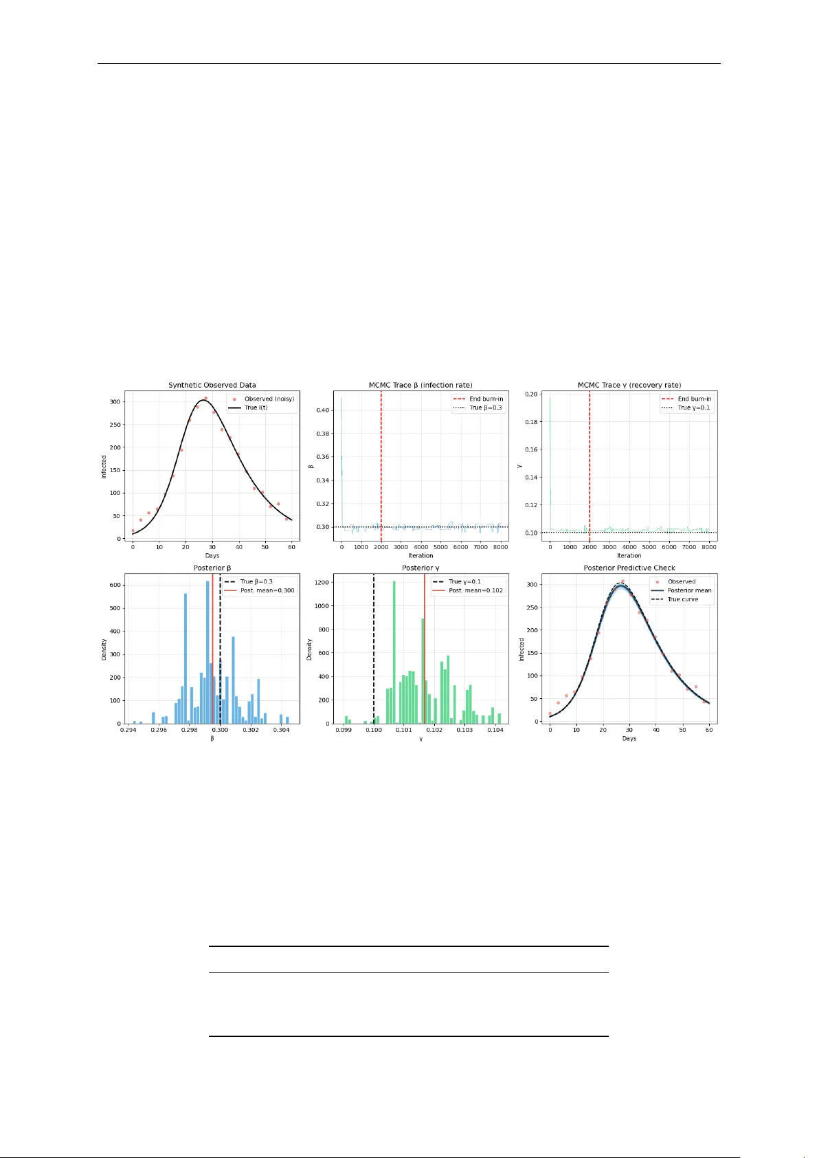
Bayesian Inference in Epidemic Modelling: A Beginner ’ s Guide Illustrated with the SIR Model Authored by Augustine Okolie PhD Mathematics “All models are wr ong but some are useful. Bayesian inference tells us how useful and how wr ong .” George E.P . Box Lecture Notes · Mathematical Epidemiology · Bayesian Statistics A Beginner ’s Guide to Bayesian Inference in Epidemic Modelling Introductory Notes 0 Contents 1 Why Do W e Need Bayesian Inference? 2 2 The SIR Model 2 2.1 Solving the ODE: From Equations to Epidemic Curves . . . . . . . . . . . . . . . 3 2.2 Interpreting the SIR Dynamics . . . . . . . . . . . . . . . . . . . . . . . . . . . . . 4 3 Bayesian Inference Setup 5 3.1 Specifying the Likelihood . . . . . . . . . . . . . . . . . . . . . . . . . . . . . . . . 6 3.1.1 The noise model . . . . . . . . . . . . . . . . . . . . . . . . . . . . . . . . . 6 3.1.2 Deriving the log-likelihood . . . . . . . . . . . . . . . . . . . . . . . . . . . 6 3.2 Specifying the Prior . . . . . . . . . . . . . . . . . . . . . . . . . . . . . . . . . . . . 7 4 Markov Chain Monte Carlo (MCMC) 7 4.1 The core idea . . . . . . . . . . . . . . . . . . . . . . . . . . . . . . . . . . . . . . . . 7 4.2 The Metropolis-Hastings Algorithm . . . . . . . . . . . . . . . . . . . . . . . . . . 8 4.3 Why does this work? . . . . . . . . . . . . . . . . . . . . . . . . . . . . . . . . . . . 8 4.4 Burn-in . . . . . . . . . . . . . . . . . . . . . . . . . . . . . . . . . . . . . . . . . . . 8 5 MCMC Results and Discussion 8 5.1 Example . . . . . . . . . . . . . . . . . . . . . . . . . . . . . . . . . . . . . . . . . . 9 5.1.1 Setup . . . . . . . . . . . . . . . . . . . . . . . . . . . . . . . . . . . . . . . . 9 5.1.2 Results . . . . . . . . . . . . . . . . . . . . . . . . . . . . . . . . . . . . . . . 9 5.2 Discussing the Results . . . . . . . . . . . . . . . . . . . . . . . . . . . . . . . . . . 10 5.3 Credible Intervals vs Confidence Intervals . . . . . . . . . . . . . . . . . . . . . . . 10 5.4 Beyond Metropolis-Hastings . . . . . . . . . . . . . . . . . . . . . . . . . . . . . . 11 5.5 Summary and Key T akeaways . . . . . . . . . . . . . . . . . . . . . . . . . . . . . . 11 Authored by Augustine Okolie (Ph.D) Email: austinefrank14@gmail.com Google Scholar All Python codes are available upon r equest 1 A Beginner ’s Guide to Bayesian Inference in Epidemic Modelling Introductory Notes 1 Why Do W e Need Bayesian Inference? When we build an epidemiological model, say , for COVID-19, influenza or Ebola, we face a fundamental challenge: we do not know the model’ s parameters θ . How infectious is the pathogen? How quickly do people recover? These are the numbers that drive the model, yet they must be inferred fr om noisy , unobserved or incomplete data. There ar e two broad philosophies for doing this. Frequentist approach Bayesian approach Find the single “best” parameter value (e.g. maximum likelihood). Find the full distribution of plausible param- eter values. Reports a point estimate, perhaps with a confidence interval. Reports a posterior distribution , a curve showing how credible each parameter value is. Cannot easily incorporate prior knowledge. Formally combines prior knowledge with new data. Asks: “What is ˆ θ ?” Asks: “What is P ( θ | data ) ?” The Key Intuition Imagine you are trying to guess the weight of a person you have never met. Before seeing any data, you alr eady know something: people rar ely weigh 5 kg or 500 kg. That is your prior . Then you observe their height and build. That is your data (likelihood). Bayesian inference combines both into a posterior , your updated, data-informed belief about their weight. 2 The SIR Model The Susceptible-Infected-Recovered (SIR) model is the workhorse of compartmental epidemiol- ogy . It divides a population of size N into thr ee groups: S usceptible I nfectious R ecovered β S I / N γ I The dynamics are governed by a system of or dinary differ ential equations (ODEs): d S d t = − β S I N , (1) d I d t = β S I N − γ I , (2) d R d t = γ I . (3) Authored by Augustine Okolie (Ph.D) Email: austinefrank14@gmail.com Google Scholar All Python codes are available upon r equest 2 A Beginner ’s Guide to Bayesian Inference in Epidemic Modelling Introductory Notes Parameters • β is the transmission rate : how quickly susceptibles become infected per contact. • γ is the recovery rate : the fraction of infected individuals who recover per unit time. • R 0 = β / γ is the basic reproduction number : average new infections caused by one case in a fully susceptible population. If R 0 > 1, the epidemic grows. Each compartment repr esents a distinct epidemiological state that every individual occupies at any given time: • Susceptible S ( t ) : individuals who have never been infected at time t and have no immu- nity . They are at risk of contracting the disease upon contact with an infectious person. At the start of an outbreak, nearly the entir e population sits in this compartment. • Infectious I ( t ) : individuals who are currently infected at time t and capable of transmitting the pathogen to susceptible individuals. The size of this compartment at any moment determines the force of infection driving the epidemic. In the basic SIR model, we assume that all infectious individuals are equally and immediately infectious, no latency period. • Recovered R ( t ) : individuals who have clear ed the infection at time t and are assumed to have acquir ed permanent immunity . They can neither be reinfected nor transmit the disease. In some diseases this is a reasonable approximation (e.g. measles); in others (e.g. influenza, COVID-19) immunity wanes over time, requiring extended models such as SIRS or SEIRS. The arrows in the schematic r epresentation of the standar d SIR model (Figure 2 ) show the only permitted transitions: S → I (infection) and I → R (recovery). There is no return path from R to S , and no direct r oute from S to R , every individual must pass through the infectious state. The rates labelling the arrows, β S I / N and γ I , are pr ecisely the terms that appear in the ODEs 1 – 3 . 2.1 Solving the ODE: From Equations to Epidemic Curves The system of equations ( 1 ) , ( 3 ) has no closed-form analytical solution. Instead, we use numerical integration : starting fr om initial conditions, we approximate the solution by taking many small time steps, updating each compartment at every step. The Euler idea (intuition) The simplest intuition comes from Euler ’s method. If we know the state at time t , we can approximate the state a small step ∆ t later by multiplying the current rate of change by the step size and adding it to the current value S ( t + ∆ t ) ≈ S ( t ) + d S d t ∆ t = S ( t ) − β S ( t ) I ( t ) N ∆ t , (4) I ( t + ∆ t ) ≈ I ( t ) + d I d t ∆ t = I ( t ) +  β S ( t ) I ( t ) N − γ I ( t )  ∆ t , (5) R ( t + ∆ t ) ≈ R ( t ) + d R d t ∆ t = R ( t ) + γ I ( t ) ∆ t . (6) Notice the internal consistency: whatever leaves S in the first equation immediately enters I in the second, and whatever leaves I via recovery immediately enters R in the third. The total population S + I + R = N is therefor e conserved at every step, no one is created or destr oyed, only moved between compartments. Authored by Augustine Okolie (Ph.D) Email: austinefrank14@gmail.com Google Scholar All Python codes are available upon r equest 3 A Beginner ’s Guide to Bayesian Inference in Epidemic Modelling Introductory Notes The step size ∆ t controls the trade-off between speed and accuracy . A large ∆ t is fast but accumulates errors; a small ∆ t is accurate but slow . In practice we use more sophisticated solvers such as Runge-Kutta 4 (RK4) , which evaluates the slope at four intermediate points within each step and takes a weighted average. The idea is identical to Euler , follow the slope, step by step , but with a much mor e accurate estimate of which slope to follow . The scipy function odeint in Python uses an adaptive version of this internally , automatically shrinking ∆ t in regions wher e the solution changes rapidly (e.g. near the epidemic peak) and enlarging it wher e the solution is flat. 2.2 Interpreting the SIR Dynamics Numerical solution and epidemic curves Figure 1: Numerical solution of the SIR model. N = 1000, I ( 0 ) = 10, S ( 0 ) = 990, R ( 0 ) = 0, with β = 0.3, γ = 0.1, R 0 = 3.0. As shown in Figur e 1 , the numerical solution reveals three compartments evolving over time and the sensitivity of the epidemic curve to the underlying parameters. Left panel: the three compartments . Three featur es stand out. First, S ( t ) declines monotonically , once infected, people do not return to the susceptible pool. Second, I ( t ) rises, peaks, then falls: the peak occurs precisely when S ( t ∗ ) = N γ β , i.e. when ther e are no longer enough susceptibles to sustain exponential growth. At this point the rate of new infections exactly equals the rate of r ecoveries, and the infectious curve turns over . Third, R ( t ) rises sigmoidally and plateaus at the final epidemic size , the total fraction of the population ever infected ( Kermack and McKendrick , 1927 ). Importantly , this plateau is strictly below N : some susceptibles always escape infection, pr otected by the declining pool of infectious individuals near the end of the outbreak. Right panel: the role of R 0 and the β - γ interplay . V arying β and γ while tracking I ( t ) reveals that R 0 is not controlled by either parameter alone, but by their ratio . Recall that 1 / γ is the mean infectious period (in days). During that window , an infected individual transmits at rate β , so: R 0 = β × 1 γ = transmission rate recovery rate This creates a natural tension between the two parameters (See T able 1 ): Authored by Augustine Okolie (Ph.D) Email: austinefrank14@gmail.com Google Scholar All Python codes are available upon r equest 4 A Beginner ’s Guide to Bayesian Inference in Epidemic Modelling Introductory Notes Disease β γ 1/ γ (days) R 0 Reference Our SIR example 0.30 0.10 10 3.0 — Seasonal flu 0.50 0.33 3 1.5 Biggerstaff et al. ( 2014 ) COVID-19 (early) 0.25 0.10 10 2.5 Liu et al. ( 2020 ) Measles 1.50 0.07 14 ≈ 15 Guerra et al. ( 2017 ) Ebola 0.20 0.10 10 ≈ 2 Althaus ( 2014 ) T able 1: R 0 estimates across diseases. Notice that measles achieves its explosive R 0 ≈ 15 through a combination of very high β and a long infectious period. Ebola, despite being lethal, has a modest R 0 because patients are quickly isolated or die, drastically shortening the ef fective infectious window ( Althaus , 2014 ). • A highly contagious but short-lived infection (large β , large γ ) can have a low R 0 , the host recovers befor e spreading widely . • A moderately contagious but prolonged infection (moderate β , small γ ) can have a high R 0 , the long infectious window compensates for slower per-contact transmission. • Only when β dominates γ , i.e. transmission outpaces recovery , does R 0 > 1 and the epidemic grow . Higher R 0 produces a taller , earlier epidemic peak and a lar ger final size ( Keeling and Rohani , 2008 ). Crucially , two parameter pairs with the same R 0 but differ ent β and γ produce dif ferent curve shapes: a higher γ compresses the infectious period and sharpens the peak even when R 0 is unchanged. R 0 alone therefor e does not fully characterise epidemic dynamics, the individual rates matter too. Key Questions & T akeaway The epidemic curve is the visible fingerprint of the hidden parameters β and γ . But how do we recover those parameters fr om noisy outbreak data? This is where Bayesian inference comes in: rather than seeking a single best estimate, it asks for the full distribution of parameter values that ar e consistent with the data and our prior knowledge, the posterior distribution . The practical challenge is that this posterior cannot be computed dir ectly , because it requir es evaluating an intractable integral over all possible parameter values. Markov Chain Monte Carlo (MCMC) is the computational engine that solves this problem. It explores the parameter space ( β , γ ) by running a chain of random proposals, accepting combinations that improve the posterior probability and occasionally accepting worse ones to avoid getting trapped at a single solution. Over many iterations, the chain maps out the full posterior distribution without ever needing to evaluate the intractable integral directly . In this way , Bayesian infer ence provides the statistical framework - what we want to compute - and MCMC provides the algorithm - how we compute it. The ODE solver sits at the heart of both: every time MCMC pr oposes a new ( β , γ ) , the solver runs the SIR model forward and compares the resulting curve to the observed case counts, scoring how plausible that parameter combination is. 3 Bayesian Inference Setup Let θ = ( β , γ ) denote the unknown parameters (i.e, the infection and recovery parameters we wish to estimate) and y the observed data (daily infected counts). The Bayes’ theorem states: Authored by Augustine Okolie (Ph.D) Email: austinefrank14@gmail.com Google Scholar All Python codes are available upon r equest 5 A Beginner ’s Guide to Bayesian Inference in Epidemic Modelling Introductory Notes P ( θ | y ) | { z } posterior = P ( y | θ ) | { z } likelihood · P ( θ ) | { z } prior P ( y ) | { z } evidence Each term has a concrete meaning in our epidemic setting: T erm Meaning in the SIR context P ( θ ) Our prior belief about β and γ befor e seeing any case data. P ( y | θ ) The likelihood : how probable are the observed counts if the true pa- rameters were θ ? P ( θ | y ) The posterior : our updated belief after seeing the outbreak data. P ( y ) A normalising constant, the same for all θ , so often ignor ed. The Problem Computing P ( y ) = R P ( y | θ ) P ( θ ) d θ requir es integrating over all possible parameter values . For the SIR model, this integral has no closed form. This is why we need MCMC. 3.1 Specifying the Likelihood 3.1.1 The noise model Real case counts ar e noisy: reporting delays, under -ascertainment, weekend effects. A simple and standard assumption is additive Gaussian noise I obs ( t ) = I model ( t ; θ ) + ε t , ε t ∼ N ( 0, σ 2 ) . That is, each observed count is the SIR model’s prediction, plus independent Gaussian noise with standard deviation σ . 3.1.2 Deriving the log-likelihood The probability of a single observation I obs ( t ) under our model is P ( I obs ( t ) | θ ) = 1 σ √ 2 π exp − [ I obs ( t ) − I model ( t ; θ ) ] 2 2 σ 2 ! . Assuming independence across time points, the joint likelihood is the pr oduct P ( y | θ ) = T ∏ t = 1 1 σ √ 2 π exp  − r 2 t 2 σ 2  , where r t = I obs ( t ) − I model ( t ; θ ) is the residual at time t . T aking the logarithm (and dropping constants that do not depend on θ ) Authored by Augustine Okolie (Ph.D) Email: austinefrank14@gmail.com Google Scholar All Python codes are available upon r equest 6 A Beginner ’s Guide to Bayesian Inference in Epidemic Modelling Introductory Notes log P ( y | θ ) ∝ − 1 2 T ∑ t = 1 r 2 t σ 2 = − 1 2 T ∑ t = 1  I obs ( t ) − I model ( t ; θ ) σ  2 . The log-likelihood is large (near zero) when the model fits well, and very negative when the model fits poorly . Connection to Least Squares Maximising the Gaussian log-likelihood over θ is identical to minimising the sum of squared residuals. Least squar es and Gaussian likelihood are the same assumption viewed from differ ent angles. Bayesian inference simply adds a prior on top and propagates the full uncertainty rather than reporting a single optimal value. 3.2 Specifying the Prior In our example we use a uniform (flat) prior over biologically sensible ranges β ∼ Uniform ( 0.05, 1.0 ) , γ ∼ Uniform ( 0.01, 0.5 ) . These ranges encode only weak prior knowledge: we know both parameters must be positive and not astronomically lar ge. In log-space log P ( θ ) = ( 0 if θ ∈ support − ∞ otherwise . Returning − ∞ in log-space means zer o probability , the MCMC sampler will never visit these regions. Choosing Priors in Practice Flat priors ar e a reasonable starting point, but informative priors can be very valuable when external data exist (e.g. serial interval studies constrain γ , contact surveys constrain β ). A well-chosen prior stabilises infer ence when data are sparse and naturally embeds domain knowledge. 4 Markov Chain Monte Carlo (MCMC) 4.1 The core idea W e cannot evaluate P ( y ) , so we cannot compute the posterior directly . But we do not need to. W e only need to draw samples from the posterior . Once we have samples θ ( 1 ) , θ ( 2 ) , . . . , θ ( M ) , we can estimate any quantity of interest, e.g E [ β | y ] ≈ 1 M M ∑ i = 1 β ( i ) , V ar [ β | y ] ≈ 1 M M ∑ i = 1  β ( i ) − ¯ β  2 . MCMC does this by building a Markov chain , a sequence of parameter values wher e each value depends only on the previous one, whose long-r un distribution is the target posterior . Authored by Augustine Okolie (Ph.D) Email: austinefrank14@gmail.com Google Scholar All Python codes are available upon r equest 7 A Beginner ’s Guide to Bayesian Inference in Epidemic Modelling Introductory Notes 4.2 The Metropolis-Hastings Algorithm Algorithm: Metropolis-Hastings 1. Initialise : Choose starting values θ ( 0 ) . 2. Propose : Draw θ ′ ∼ q ( θ ′ | θ ( t ) ) , e.g. a Gaussian random walk β ′ = β ( t ) + ε β , γ ′ = γ ( t ) + ε γ , ε ∼ N ( 0, δ 2 ) 3. Accept or reject : Compute the acceptance ratio α = min  1, P ( θ ′ | y ) P ( θ ( t ) | y )  = min  1, P ( y | θ ′ ) P ( θ ′ ) P ( y | θ ( t ) ) P ( θ ( t ) )  Note: P ( y ) cancels! Set θ ( t + 1 ) = θ ′ with probability α , else θ ( t + 1 ) = θ ( t ) . 4. Repeat for t = 1, 2, . . . , N iter . The key insight in Step 3 is profound: since P ( y ) appears in both numerator and denominator , it cancels out entirely . W e never need to compute the intractable normalising constant. 4.3 Why does this work? • If the pr oposed θ ′ has higher posterior pr obability than the curr ent θ ( t ) : always accepted ( α = 1). The chain moves uphill. • If θ ′ has lower posterior probability: accepted with probability α < 1. The chain occasionally moves downhill. This occasional downhill movement is essential, it allows the chain to explore the full posterior shape rather than simply converging to a single peak. Over many iterations, the fraction of time the chain spends near any parameter value is proportional to that value’s posterior pr obability . 4.4 Burn-in The chain starts fr om an arbitrary point θ ( 0 ) and takes some time to r each the high-probability region of the posterior . Samples collected during this initial “warm-up” period ar e discarded. This is called the burn-in period. θ ( 0 ) , θ ( 1 ) , . . . , θ ( B ) | { z } burn-in (discard) , θ ( B + 1 ) , . . . , θ ( N ) | { z } posterior samples (keep) Intuition for the Whole Algorithm Think of the posterior surface as a hilly landscape wher e altitude r epresents pr obability . The Metropolis-Hastings algorithm is like a hiker who always climbs uphill but occasionally stumbles downhill. Over time, the hiker spends most of their time near the peaks (high- probability regions) but occasionally visits the valleys too. The density of the hiker ’s footprints is a map of the posterior distribution. 5 MCMC Results and Discussion Authored by Augustine Okolie (Ph.D) Email: austinefrank14@gmail.com Google Scholar All Python codes are available upon r equest 8 A Beginner ’s Guide to Bayesian Inference in Epidemic Modelling Introductory Notes 5.1 Example W e now walk through a complete implementation. W e simulate synthetic outbreak data and then recover the parameters via MCMC, mimicking the real-world task of fitting a model to surveillance data. 5.1.1 Setup • Population: N = 1000, initially I 0 = 10 infected. • T rue parameters: β ∗ = 0.3, γ ∗ = 0.1 ⇒ R ∗ 0 = 3.0. • Observed data: SIR simulation + Gaussian noise ( σ = 15). • Prior: β ∼ U ( 0.05, 1.0 ) , γ ∼ U ( 0.01, 0.5 ) . • MCMC: 8000 iterations, step size δ = 0.015, burn-in of 2000. Figure 2: MCMC output for the SIR parameter estimation problem ( N = 1000, β ∗ = 0.3, γ ∗ = 0.1, R ∗ 0 = 3.0, 8000 iterations, burn-in = 2000). T op r ow , left to right : noisy observed infected counts against the true epidemic curve; MCMC trace for β ; MCMC trace for γ . Bottom row , left to right : posterior distribution of β ; posterior distribution of γ ; posterior predictive check showing 100 SIR trajectories drawn from the posterior against the observed data. 5.1.2 Results After discarding the burn-in, the posterior means r ecovered the tr ue parameters accurately: Parameter T rue value Posterior mean Posterior std. β 0.300 0.300 0.002 γ 0.100 0.102 0.001 R 0 = β / γ 3.00 2.95 0.03 Authored by Augustine Okolie (Ph.D) Email: austinefrank14@gmail.com Google Scholar All Python codes are available upon r equest 9 A Beginner ’s Guide to Bayesian Inference in Epidemic Modelling Introductory Notes The narr ow posterior standard deviations reflect the informativeness of 60 days of daily data. More noise, fewer data points or a less identifiable model would pr oduce wider posteriors. 5.2 Discussing the Results Figure 2 summarises the full MCMC output. Panel 1 (top left) - observed data: The noisy red dots are the synthetic observed infected counts, generated by adding Gaussian noise ( σ = 15) to the true SIR trajectory . The black curve is the ground truth. This panel contextualises the inference pr oblem: the MCMC algorithm sees only the noisy dots and must work backwards to recover the parameters that plausibly generated them. The gap between the dots and the true curve repr esents the irreducible observational uncertainty that the posterior will absorb. Panels 2 and 3 (top centre and right) - trace plots: The trace plots show the chain’s path through β and γ values over all 8000 iterations. A well-behaved chain resembles a dense, fast-mixing caterpillar , bouncing rapidly ar ound a stable r egion with no long-range drifts or flat stretches. The red dashed vertical line marks the end of the burn-in period (iteration 2000), after which the chain is considered to have converged to the stationary distribution. Samples before this line are discarded. T wo warning signs to watch for in practice: if the chain drifts slowly acr oss the plot, it has not converged and mor e iterations are needed; if it gets stuck for long stretches at a single value, the proposal step size δ is too lar ge and nearly all proposals ar e being r ejected. A healthy acceptance rate lies roughly between 20% and 40% for a two-parameter random walk Metr opolis sampler . Panels 4 and 5 (bottom left and centre) - posterior distributions: The histograms of post-burn- in samples are the central deliverable of Bayesian inference: they are the posterior distributions of β and γ . Several features deserve attention. The peaks of both histograms sit very close to the true values ( β ∗ = 0.3, γ ∗ = 0.1), confirming that the inference is accurate. The widths of the distributions quantify posterior uncertainty: narrow peaks indicate that the data ar e highly informative about the parameter , while wide peaks indicate that many parameter values remain plausible after seeing the data. In our example the posteriors are tight because 60 days of daily counts provide str ong constraints. W ith noisier data, fewer observations or a shorter outbr eak window , the posteriors would br oaden, and the Bayesian framework captures this automatically , without any additional modelling effort. Panel 6 (bottom right) - posterior predictive check: The posterior predictive check is the ultimate model validation tool. One hundred ( β , γ ) pairs are drawn at random from the posterior and each is used to simulate a full SIR trajectory . The resulting blue band r epresents the full range of epidemic curves that are consistent with both the data and our model assumptions. If the observed data points fall comfortably within this band, the model is a cr edible explanation of the outbreak. If the data systematically fall outside the band, the model is misspecified, perhaps the SIR assumption of permanent immunity is violated or the population is structur ed in ways the model ignores. The posterior predictive check ther efore bridges parameter estimation and model criticism, and should always be reported alongside the posterior summaries ( Gelman et al. , 2013 ). 5.3 Credible Intervals vs Confidence Intervals A 95% credible interval [ a , b ] means: P ( a ≤ β ≤ b | y ) = 0.95 There is a 95% pr obability , given the data and our prior , that β lies between a and b . This is the direct, intuitive statement most practitioners want. Authored by Augustine Okolie (Ph.D) Email: austinefrank14@gmail.com Google Scholar All Python codes are available upon r equest 10 A Beginner ’s Guide to Bayesian Inference in Epidemic Modelling Introductory Notes A 95% frequentist confidence interval does not mean this. It means: if we repeated the experi- ment many times, 95% of such intervals would contain the true value. This is a subtle and often misunderstood distinction. In practice, for flat priors and large samples, cr edible intervals and confidence intervals tend to agree numerically , but their interpretations r emain fundamentally differ ent. 5.4 Beyond Metropolis-Hastings The Metropolis-Hastings algorithm is the conceptual foundation, but modern epidemiological work uses more sophisticated samplers: Sampler Key idea and when to use it NUTS / HMC Uses gradient information to pr opose distant moves effi- ciently . The default in Stan and PyMC. Much better for higher- dimensional problems. Gibbs sampling Updates one parameter at a time from its conditional distribu- tion. Useful when conditionals have closed forms. SMC Sequential Monte Carlo, well-suited to time-series and online updating as data arrives. NUTS in Stan The practical recommendation for most SIR/SEIR fitting prob- lems. V ery few tuning parameters, excellent diagnostics. 5.5 Summary and Key T akeaways The Five Things to Remember 1. Bayesian inference is about distributions, not point estimates. The posterior P ( θ | y ) tells you the full range of plausible parameter values, not just a single best guess. 2. The three ingredients are prior , likelihood, and Bayes’ theorem. The prior encodes pre-existing knowledge; the likelihood scores how well each parameter value explains the data; their product (normalised) is the posterior . 3. The Gaussian log-likelihood is just penalised squared residuals. If you have used least squares befor e, you have implicitly assumed Gaussian noise, Bayesian inference makes this explicit. 4. MCMC avoids the intractable normalising constant. The Metropolis-Hastings accep- tance ratio cancels P ( y ) , so we can sample fr om the posterior without ever computing it. 5. Always check your trace plots and do a posterior predictive check. T race plots diag- nose sampler health; posterior predictive checks verify that the fitted model actually repr oduces the observed data. The Big Picture Epidemiological models are tools for understanding transmission dynamics and informing policy . Their parameters ar e never known exactly . Bayesian MCMC gives us a principled, computationally feasible way to say not just “our best estimate of R 0 is 2.5” but “given the data, R 0 is between 2.1 and 2.9 with 95% probability” , and that uncertainty matters enormously for intervention planning. Authored by Augustine Okolie (Ph.D) Email: austinefrank14@gmail.com Google Scholar All Python codes are available upon r equest 11 A Beginner ’s Guide to Bayesian Inference in Epidemic Modelling Introductory Notes 5 References Althaus, C.L. (2014). Estimating the r eproduction number of Ebola virus during the 2014 outbreak in W est Africa. PLOS Currents Outbreaks , 6. Biggerstaff, M., Cauchemez, S., Reed, C., Gambhir , M., and Finelli, L. (2014). Estimates of the repr oduction number for seasonal, pandemic, and zoonotic influenza: a systematic review of the literature. BMC Infectious Diseases , 14, 480. Gelman, A., Carlin, J.B., Stern, H.S., Dunson, D.B., V ehtari, A., and Rubin, D.B. (2013). Bayesian Data Analysis , 3rd ed. Chapman & Hall/CRC. Guerra, F .M., Bolotin, S., Lim, G., Heffernan, J., Deeks, S.L., Li, Y ., and Cr owcroft, N.S. (2017). The basic repr oduction number (R 0 ) of measles: a systematic review . The Lancet Infectious Diseases , 17(12), e420–e428. Keeling, M.J. and Rohani, P . (2008). Modeling Infectious Diseases in Humans and Animals . Princeton University Press. Kermack, W .O. and McKendrick, A.G. (1927). A contribution to the mathematical theory of epidemics. Proceedings of the Royal Society A , 115(772), 700–721. Liu, Y ., Gayle, A.A., W ilder-Smith, A., and Rockl ¨ ov , J. (2020). The reproductive number of COVID-19 is higher compared to SARS cor onavirus. Journal of T ravel Medicine , 27(2), taaa021. Authored by Augustine Okolie (Ph.D) Email: austinefrank14@gmail.com Google Scholar All Python codes are available upon r equest 12