Fluids You Can Trust: Property-Preserving Operator Learning for Incompressible Flows

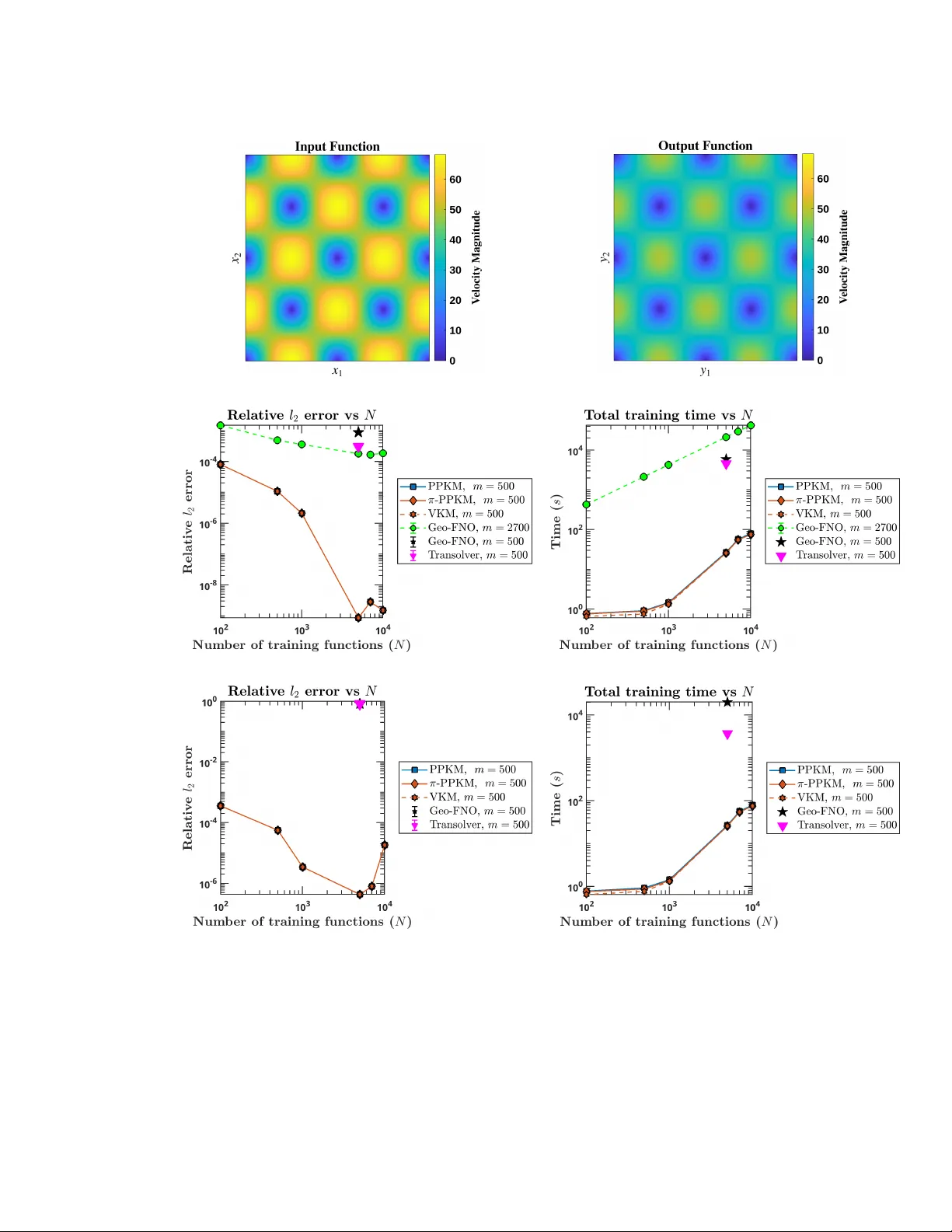
Fluids Y ou Can T rust: Prop ert y-Preserving Op erator Learning for Incompressible Flo ws Ramansh Sharma ramansh@cs.ut ah.edu Kahlert Scho ol of Computing University of Utah UT, USA Matthew Lo w ery mlo wer y@cs.ut ah.edu Kahlert Scho ol of Computing University of Utah UT, USA Houman Owhadi o whadi@cal tech.edu Dep artment of Computing and Mathematic al Scienc es California Institute of T e chnolo gy CA, USA V arun Shank ar shankar@cs.ut ah.edu Kahlert Scho ol of Computing University of Utah UT, USA Abstract W e presen t a no vel prop ert y-preserving kernel-based op erator learning metho d for incom- pressible ﬂo ws gov erned b y the incompressible Na vier–Stokes equations. T raditional n u- merical solv ers incur signiﬁcant computational costs to respect incompressibility . Op erator learning oﬀers eﬃcien t surrogate mo dels, but current neural op erators fail to exactly en- force ph ysical prop erties suc h as incompressibility , p erio dicit y , and turbulence. Our k ernel metho d maps input functions to expansion co eﬃcien ts of output functions in a prop erty- preserving k ernel basis, ensuring that predicted velocity ﬁelds analytic al ly and simulta- ne ously preserv e the aforementioned physical properties. Our metho d leverages eﬃcient n umerical linear algebra, simple ro otﬁnding, and streaming to allow for training at-scale on desktop GPUs. W e also presen t universal approximation results and b oth p essimistic and more realistic a priori con vergence rates for our framew ork. W e ev aluate the metho d on c hallenging 2D and 3D, laminar and turbulen t, incompressible ﬂo w problems. Our metho d achiev es up to six orders of magnitude low er relative ℓ 2 errors up on generalization and trains up to ﬁv e orders of magnitude faster compared to neural op erators, despite our metho d b eing trained on desktop GPUs and neural op erators b eing trained on cutting-edge GPU serv ers. Moreov er, while our metho d enforces incompressibility analytically , neural op erators exhibit v ery large deviations. Our results show that our metho d provides an accurate and eﬃcient surrogate for incompressible ﬂo ws. Keyw ords: op erator learning, surrogate mo deling, incompressible ﬂo w, kernel metho ds 1 Introduction Incompressible ﬂuid ﬂo ws arise in an enormous range of engineering and scientiﬁc applica- tions, suc h as the study of ﬂo w past airfoils & wings (Thw aites and Street, 1960), aero dynam- © 2026 Sharma, Lo wery , Owhadi, and Shank ar. License: CC-BY 4.0, see https://creativecommons.org/licenses/by/4.0/ . Sharma, Lower y, Owhadi, and Shankar ics (K wak et al., 1986; Chang et al., 1988; Kw ak and Kiris, 2009), weather prediction (Cas- torrini et al., 2023), c hemical mixing (Na jm and Knio, 2005), and hemo dynamics (Janela et al., 2010; Canic and Mikelic, 2003; Secom b, 2016; W omersley, 1955; McDonald, 1955; P erktold and Rappitsch, 1995). These ﬂows are typically mo deled with the incompressible Na vier–Stokes (INS) equations giv en by: B u B t + ( u ⋅ ∇ ) u = ν ∇ 2 u − 1 ρ ∇ p + 1 ρ f , on Ω × ( 0 , T ] , (1) ∇ ⋅ u = 0 , on Ω × ( 0 , T ] , (2) B u = g , on B Ω × ( 0 , T ] , (3) u ( x , 0 ) = u 0 ( x ) , on Ω , (4) where u is the divergence-free v elo cit y ﬁeld, p is the pressure, ν is the kinematic viscos- it y , ρ is the ﬂuid density , f is the external b o dy forces, B denotes the b oundary op erator, and u 0 and g are the initial and b oundary conditions resp ectiv ely . These equations con- stitute a system of nonlinear partial diﬀeren tial equations (PDEs) and encompass a v ariet y of ph ysical phenomena suc h as b oundary la y ers, v ortex dynamics, ﬂow separ ation, and turbulence. The challenging nature of these PDEs necessitates sp ecialized numerical dis- cretizations of whic h there are four dominan t classes: (1) saddle-p oin t metho ds, which solve the coupled PDE system directly and reach arbitrary orders of accuracy (Orszag et al., 1986; Karniadakis et al., 1991; John, 2002; Ahmed et al., 2018); (2) high-order metho ds that treat the pressure explicitly and recov er it via the pressure Poisson equation (“PPE” metho ds) (Johnston and Liu, 2004; John, 2002; Rosales et al., 2021); (3) artiﬁcial compress- ibilit y metho ds (Chorin, 1967; Guermond and Minev, 2015); and (4) temp orally lo w-order pro jection-based metho ds (Chorin and Marsden, 1993; Bro wn et al., 2001; Go da, 1979; v an Kan, 1986; Bell et al., 1989; Guy and F ogelson, 2005; Guermond et al., 2006). All of these metho ds come with their o wn computational b ottlenec ks, t ypically requiring problem- sp eciﬁc preconditioners (Elman, 2002; John, 2002; Ahmed et al., 2018), exp ensiv e P oisson solv es (Johnston and Liu, 2004; Jung et al., 2013; Dic k et al., 2015) or vector Helmholtz solv es (Guermond and Minev, 2015, 2017). F urther, explicit treatmen t of the nonlinear adv ection term leads to the Courant–F riedrichs–Lewy (CFL) stability constrain t, severely limiting admissible time-step size (Kress and Lötstedt, 2006). These issues ha ve led to a gro wing in terest in developing surr o gate mo dels that can reduce the cost of obtaining solu- tions for new problem conﬁgurations (Ionita and An toulas, 2014; Ohlb erger and Rav e, 2015; T ezzele et al., 2020; Bhattachary a et al., 2021). Surrogate mo dels for PDEs include reduced order mo dels (Holmes et al., 2012; Quarteroni et al., 2016), machine learning (ML) based metho ds (Lee and Carlberg, 2020; F resca et al., 2020; Sirignano and Spiliopoulos, 2018; Th uerey et al., 2020; Sanchez-Gonzalez et al., 2020; Pfaﬀ et al., 2020; Raissi et al., 2019). More recently , op erator learning models (Boullé and T o wnsend, 2024) that act directly on function spaces ha ve emerged as a comp etitiv e class of surrogates. Operator learning seeks to appro ximate the solution op er ator of the PDE as a mapping from input functions (geom- etry , PDE parameters, initial conditions, and/or b oundary conditions) to output functions (solutions). Prominent neural operator architectures include deep op erator netw orks (Deep- ONets) (Lu et al., 2021), which train t wo separate neural net work in conjunction; F ourier neural op erators (FNOs) (Li et al., 2020a) and their geometrically-ﬂexible v arian ts such as 2 Tr ustwor thy Fluids Figure 1: Sc hematic diagram of the prop osed prop ert y-preserving kernel method. the Geo-FNO (Li et al., 2020a), whic h in volv e k ernel-based in tegral operators computed implicitly via the fast F ourier transform(FFT); the kernel neural op erator (KNO) (Low ery et al., 2024) which uses explicit k ernels and quadrature instead of the FFT; deep Green net- w orks (DGN) (Gin et al., 2021; Boullé et al., 2022) and their graph neural op erator (GNO) coun terparts (Li et al., 2020b), which aim to learn the Green’s k ernel either globally or lo cally; and more recen tly , transformer-based neural op erators that lev erage the attention mec hanism (Hao et al., 2023; Liu et al., 2025, 2024). Complementary to these methods, recen t w ork Batlle et al. (2024); Mora et al. (2025) has shown that kernel/Gaussian pro cess (GP) regression can b e comp etitiv e for op erator learning as well. Kernel methods for op- erator learning are meshless and typically use only a single trainable parameter; note that op erator-v alued k ernels w ere ﬁrst in tro duced in Kadri et al. (2011, 2016). Despite these adv ances, to the b est of our knowledge, current op erator learning techniques are unable to analytic al ly and simultane ously satisfy multiple ﬂuid properties such as incompressibility , p eriodicity , and turbulence-related p o wer laws. Recen t attempts in this direction with ei- ther soft constrain ts (Gosw ami et al., 2022; Li et al., 2023a, 2024; Zhang et al., 2025) or hard constraints Rich ter-P ow ell et al. (2022); Khorrami et al. (2024) hav e only succeeded in appro ximate enforcement of incompressibility . Unfortunate ly , a surrogate that fails to ana- lytically satisfy these prop erties can pro duce physically-inconsisten t predictions, accumulate spurious divergence, or b e unable to replicate key ﬂow features even if its p oin twise errors are small. In this work, we address this gap b y in tro ducing a nov el prop ert y-preserving k ernel-based op erator learning metho d for incompressible ﬂows. Unlik e the k ernel metho d in Batlle et al. (2024), we learn a map from input function samples to interp olation c o eﬃcients asso ciated with output functions, where these co eﬃcien ts are asso ciated with a kernel basis that is analytically prop ert y-preserving. Our framew ork uses t wo k ernel interpolants: (1) one that in terp olates the output functions using a prop ert y-preserving kernel basis, and (2) one that consumes input functions and ﬁts the interpolation coeﬃcients from (1). The resulting metho d only uses t wo trainable parameters. This approac h decouples p oin twise generaliza- tion errors in our surrogate mo dels from their abilit y to resp ect physical constrain ts; while the former still dep ends on the training data, the latter is alwa ys guaran teed to mac hine precision; see Figure 1 for an illustration of our metho d. W e illustrate the capabilities of our metho d with extensive numerical exp eriments on an extensiv e suite of 2D and 3D problems inv olving incompressible ﬂo ws. W e construct sur- 3 Sharma, Lower y, Owhadi, and Shankar rogates that are all analytically incompressible on generalization, but that also analytically satisfy p eriodicity or turbulence-related pow er laws when applicable. A cross these problems, w e compare our metho d against the v anilla kernel metho d in Batlle et al. (2024), and t wo state-of-the-art neural op erator baselines, Geo-FNO (Li et al., 2023b) and T ransolv er (W u et al., 2024). The resulting metho d is meshless; interpretable; t ypically orders of magnitude more accurate than existing neural operator approac hes ev en in point wise generalization errors; analytically prop ert y-preserving (if the prop erties are known in adv ance); more eﬃ- cien t than neural op erators in terms of trainable parameter counts (tw o for our metho d vs millions for neural op erators); and orders of magnitude faster in terms of training time. The remainder of the pap er is organized as follows. In Section 2, w e present an ov erview of op erator learning and both the high-lev el algorithm and the mathematical form ulation of the prop ert y-preserving k ernel metho d, with a fo cus on incompressibility , p erio dicit y , and turbulence-related p o wer laws. In Section 3, we then presen t approximation theorems regarding univ ersal approximation and conv ergence rates of the metho d. W e present results of n umerical exp erimen ts in Section 4, comparing our metho d against comp etitors in terms of accuracy , div ergence, and runtime. Finally , in Section 5, w e discuss the implications of the results in detail and discuss future directions. 2 A Prop erty-Preserving Kernel Metho d for Op erator Learning In this section, we present an o verview of op erator learning (Section 2.1), then present the high-lev el algorithm used in this work (Section 2.2), and then describ e the mathematical form ulation and implemen tation details of the prop ert y-preserving kernel metho d (Section 2.3 – 2.5.3). 2.1 Ov erview of Op erator Learning W e no w brieﬂy describ e k ernel-based op erator learning. Let A and V b e t wo separable Banac h spaces of functions and let G ∶ A → V b e an operator that maps functions a ∈ A (input functions) to functions v ∈ V (output functions), i.e. G ( a ) = v . The goal of op erator learning is to learn an approximation ˜ G ≈ G giv en N pairs of input and output functions, {( a i , v i )} , i = 1 , . . . , N . Let Ω a and Ω v b e the domains for the input and output functions resp ectiv ely . The choice of these domains is arbitrary; they can b e spatial, spatiotemp oral, or parametric, for instance. In practice, the functions are pro vided as a ﬁnite n umber of samples on their respective domains; let n and m denote the num b er of samples provided for the input and output functions, resp ectiv ely . F urther, in the most general setting and the setting of this w ork, the functions can be v ector-v alued so that a ∶ Ω a → R p and v ∶ Ω v → R d . In this w ork, we will fo cus on a k ernel-based parametrization of ˜ G , a generalization of the w ork b y Batlle et al. (2024).The k ernel metho d for operator learning (ﬁrst prop osed by Batlle et al. (2024)) formulates ˜ G as v ≈ ˜ G ( a ) = χ ○ ˜ f ○ φ ( a ) , (5) where χ ∶ R m → V reconstructs v by in terp olating its m samples, φ ∶ A → R n generates n sam- ples of a , and ˜ f ∶ R n → R m maps from n samples of a to m samples of v . F ollowing Batlle et al. (2024), we endo w b oth A and V with repro ducing kernel Hilbert spaces (RKHSs) and 4 Tr ustwor thy Fluids c ho ose k ernel maps for χ and ˜ f . Sp eciﬁcally , we choose to w ork with p ositiv e-deﬁnite radial k ernels (also called radial basis functions or RBF s) so that, assuming pairwise distinct inter- p olation p oin ts, the linear systems in (8), (18), and (21) admit unique in terp olan ts (Chen et al., 2005; F asshauer, 2007; Baxter, 2010). 2.2 Our con tribution Algorithm 1 T raining and ev aluation procedure for the prop ert y-preserving k ernel method. Require: 1: T raining data set : N pairs of input and output function ev aluations, {( a i , v i )} N i = 1 . 2: Inference example : ( a ⋆ , v ⋆ ) is an unseen pair of input and output function ev alua- tions. 3: Prop ert y-preserving kernel Φ and op erator k ernel λ . Ridge parameter θ . Let: a ∈ R np and v ∈ R md denote the column v ectors of the training input and output function ev aluations respectively . Let: v ⋆ ∈ R m ⋆ d denote the column vector of the inference output function ev aluations at m ⋆ p oin ts. Let: Φ denote the md × md Gramian matrix asso ciated with Φ , see Section 2.3 for details. Let: K denote the N × N Gramian matrix asso ciated with λ , see Section 2.4 for details. Let: K ⋆ denote the 1 × N operator kernel ev aluation matrix and Φ ⋆ denote the m ⋆ d × md prop ert y-preserving k ernel ev aluation matrix. T raining: 1: Solve the block linear system (8) for b i , i = 1 , . . . , N using the tec hniques in Section 2.5.2. 2: Find ϵ as the ro ot of the function κ ( K ϵ ) − 10 15 using the approach outlined in Sec- tion 2.5.1. 3: Solve the linear system (22) for c j , j = 1 , . . . , md , using ϵ and θ . Generalization: 1: Obtain output co eﬃcien ts as b ⋆ ←        K ⋆ c 1 ⋮ K ⋆ c md        ∈ R md . 2: Obtain a prop ert y-preserving prediction ˜ v ⋆ ← Φ ⋆ b ⋆ . Our metho d emerges from the observ ation that if χ is carefully constructed to b e a matrix-v alued k ernel in terp olan t that analytic al ly enforces desirable prop erties (such as in- compressibilit y , p eriodicity , and turbulence) when interpolating v , then c hanging ˜ f to output expansion co eﬃcien ts in that kernel interpolant ensures that all predictions made by ˜ G ( a ) for ev ery a will automatically (and analytically) satisfy those properties as w ell. Our metho d therefore has tw o main comp onen ts; (i) the v ector-v alued op erator k ernel interpolant ˜ f , and (ii) the vector-v alued prop ert y-preserving kernel interpolant χ . W e summarize the metho d in Algorithm 1; describ e the tw o comp onen ts in detail in Sections 2.3 and 2.4; and presen t relev ant implementation details in Section 2.5. A schematic of our metho d is shown in Figure 1. A note on blo c k v ector notation : W e brieﬂy describe the vector notation used throughout this section for input and output function ev aluations. Let v ∶ R d → R d b e a 5 Sharma, Lower y, Owhadi, and Shankar v ector v alued function that is ev aluated at a set of p oin ts { y j } m j = 1 ⊂ R d . W e denote these ev aluations by the blo c k vector v =        v 1 ⋮ v d        ∈ R md , (6) where each block v k =  v k ( y 1 ) , . . . , v k ( y m )  T ∈ R m con tains the ev aluations of the k th spatial comp onen t of v . This notation is helpful when discussing vector-v alued k ernel interpolants. 2.3 The prop ert y-preserving k ernel in terp olan t W e no w discuss ho w v arious prop erties can b e analytically encoded into a kernel basis. F or this w ork, the relev an t function spaces V alw a ys consist of incompressible velocity ﬁelds whic h are solutions to PDEs such as (1). A dditionally , depending on the problem, these v elo cit y ﬁelds can also exhibit spatial p eriodicity (due to b oundary conditions) and turbu- lence (due to mo deling choices). In our metho d, w e use a prop ert y-preserving kernel basis in χ such that the v elo cit y ﬁelds recov ered analytically preserve these spatial prop erties. Let Y = { y j } m j = 1 ⊂ Ω v ⊂ R d b e a set of spatial points where an output function v ∶ R d → R d is ev aluated; further, let the blo c k vector v =  v 1 , . . . , v d  T ∈ R md denote the function ev alu- ations of v at Y . Letting Φ ∶ R d × R d → R d × d b e a matrix-v alued p ositiv e-deﬁnite prop ert y- preserving kernel (describ ed in the following subsections), we explicitly write the resulting k ernel interpolant as χ ( y ) = m ∑ j = 1 Φ ( y , y j ) b j , (7) where b j ∈ R d . In order to interpolate v , we enforce χ ( y ) = v ( y ) for all y ∈ Y . These in ter- p olation conditions giv e rise to the linear system Φb = v , (8) where Φ ij = Φ ( y i , y j ) is the md × md blo c k Gramian matrix arising from ev aluations of Φ , and b =  b 1 , . . . , b d  T ∈ R md con tains the interpolation co eﬃcien t vectors for eac h spatial comp onen t. In the op erator learning setting, there are multiple suc h target functions v i ; we denote b y b i ∈ R md the co eﬃcien t v ector for the i th output function, and b y b j i its j th comp o- nen t. The system (8) has a unique solution if the p oin ts in Y are distinct (F asshauer, 2007; W endland, 2005). This md × md system is computationally exp ensive to solve ( O ( d 3 m 3 ) op- erations for a Cholesky factorization, and O ( d 2 m 2 ) op erations for subsequen t solves for eac h righ t-hand side). Ho wev er, w e never form and store Φ , but instead compute only with the individual blo c ks in Φ , reducing the solution cost signiﬁcan tly . These details are describ ed in Section 2.5. Once the interpolation co eﬃcien ts in (7) are computed, the in terp olan t can b e ev aluated at an y lo cation (ideally within the h ull of Y ). Let Y ∗ b e a set of m ∗ ev aluation lo cations. Then, the ev aluation of χ ( y ) at Y ∗ can b e written as a matrix-vector pro duct χ ( y ) Y ∗ = Φ ∗ b , (9) 6 Tr ustwor thy Fluids where Φ ∗ ( y ∗ k , y j ) , k = 1 , . . . , m ∗ , j = 1 . . . , m is the m ∗ d × md (rectangular) ev aluation matrix. Th us far, our description of these property-preserving matrix-v alued kernels has been abstract. In the follo wing subsections, we describ e in detail ho w to sim ultaneously enco de incompressibilit y , p erio dicit y , and turbulence in Φ . 2.3.1 Incompressibility The primary goal of this work is the high-ﬁdelit y surrogate mo deling of incompressible ﬂuid ﬂo ws. T o that end, our matrix-v alued kernel Φ and the corresp onding prop ert y-preserving in terp olan t (7) alwa ys enforce incompressibility analytically . The appro ximation of divergence-free (incompressible) vector ﬁelds has a long history in the numerical metho ds and approximation literature. Classical divergence-conforming ﬁnite elemen t spaces, suc h as the Raviart–Thomas (Raviart and Thomas, 1977), Brezzi–Douglas– Marini (Brezzi et al., 1985), and Nédélec elements (Nédélec, 1980), enforce the div ergence- free constrain t b y construction through their basis functions, yielding lo cal and exactly div ergence-free n umerical solutions. This paradigm established the foundational principle of enforcing physical constrain ts b y restricting the admissible solution space. How ev er, these constructions rely on p olynomial in terp olation ov er simplices, thereb y necessitating spatial meshes. Subsequen t work in the meshfree approximation literature led to the construction of matrix-v alued divergence-free k ernels from scalar-v alued p ositiv e-deﬁnite k ernels (Narco wic h and W ard, 1994; Narcowic h et al., 2007; F uselier, 2008; F uselier et al., 2009; W endland, 2009), ev en leading to numerical metho ds for meshfree Helmholtz-Hodge decomp ositions and in- compressible ﬂow solv ers (F uselier and W right, 2017; F uselier et al., 2016; Drake et al., 2021; Owhadi, 2023). While Algorithm 1 can easily lev erage mesh-based divergence-free approxi- mations, we c ho ose to use k ernel-based metho ds as they are (1) meshfree and therefore more general; and more imp ortan tly (2) can simultane ously enc o de multiple pr op erties in addition to inc ompr essibility . W e no w describe the k ernel construction used in this work. Let ϕ ∶ R d × R d → R b e a scalar-v alued p ositiv e-deﬁnite k ernel that is at least C 4 ( R d ) . The asso ciated divergence-free matrix-v alued kernel is deﬁned by Φ ( x, y ) = ∇ y × ∇ x × ϕ ( x, y ) , (10) where the diﬀeren tial operators act comp onent wise, and x = ( x 1 , . . . , x d ) and y = ( y 1 , . . . , y d ) are p oin ts in R d . F or d = 2 , we obtain the following matrix-v alued kernel Φ ( x, y ) =  B x 2 B y 2 − B x 1 B y 2 − B x 2 B y 1 B x 1 B y 1  ϕ ( x, y ) . (11) Whereas for d = 3 we obtain Φ ( x, y ) =        B x 3 B y 3 + B x 2 B y 2 − B x 1 B y 2 − B x 1 B y 3 − B x 2 B y 1 B x 3 B y 3 + B x 1 B y 1 − B x 2 B y 3 − B x 3 B y 1 − B x 3 B y 2 B x 2 B y 2 + B x 1 B y 1        ϕ ( x, y ) . (12) By construction, each column of Φ is divergence free with resp ect to the ev aluation co ordi- nate y , and the resulting kernel is p ositiv e-deﬁnite; a simpliﬁed form is also readily a v ailable for radial kernels (F uselier et al., 2016). An imp ortan t consequence of this construction is 7 Sharma, Lower y, Owhadi, and Shankar that an y kernel in terp olan t of the form (7) lies in a divergence-free space. Consequen tly , the in terp olan t χ satisﬁes ∇ ⋅ χ = 0 p oin twise throughout the domain, indep enden tly of the sam- pling lo cations or interpolation co eﬃcien ts. This pro vides an analytically exact enforcement of incompressibilit y . 2.3.2 Periodicity In addition to incompressibility , many applications require v elo cit y ﬁelds to satisfy p erio dic b oundary conditions, typically for enabling the mo deling of larger physical domains at low er computational cost but also for mo deling truly perio dic domain geometries. Giv en that w e b egan with the div ergence-free k ernel Φ , this no w opens up the issue of additionally incorp orating perio dicity into Φ . In the kernel and RBF literature, perio dic structure is imp osed in settings ranging from in terp olation on perio dic domains (Jacob et al., 2002; F asshauer, 2007) to the n umerical treatmen t of p eriodic b oundary conditions (Nguyen et al., 2012) and closed curves (Boisson- nat and T eillaud, 2006). Existing approac hes fall in to three broad categories: F ourier-based constructions, direct kernel and RBF mo diﬁcations on p erio dic domains, and embedding- based tec hniques that enforce perio dicity by construction. F ourier spectral and pseudosp ec- tral metho ds are classical to ols for appro ximating p erio dic functions (Canuto et al., 2006; Bo yd, 2001; F ornberg, 1996), while k ernel and RBF metho ds imp ose p eriodicity via kernel p eriodization and lattice-p oin t metho ds (Xiao and Bo yd, 2014; Co ols et al., 2019; Kaarnio ja et al., 2022). Embedding-based metho ds enco de p erio dicit y through an explicit embedding of Euclidean co ordinates in to a compact manifold, most commonly the circle or torus. This idea has b een employ ed in numerical metho ds for PDEs on the sphere (Fly er and W right, 2007, 2009); for elastic surfaces in ﬂuid-structure in teraction problems in Shank ar et al. (2015); Shank ar and Olson (2015); Kassen et al. (2022); and for problems posed on tori in F uselier and W right (2015); Owhadi (2023). A dopting the em b edding-based approac h, w e enforce p eriodicity by comp osing kernels with an explicitly p eriodic embedding into a higher-dimensional Euclidean space. With this approac h, perio dicit y is enforced by construction, allo wing standard k ernel constructions to b e used without requiring k ernel p erio dization. Sp eciﬁcally , we deﬁne an em b edding h ∶ T d → R 2 d as h ( y ) = ( cos ( y 1 ) , sin ( y 1 ) , . . . , cos ( y d ) , sin ( y d )) . (13) Comp osition with h induces 2 π -p eriodicity in each spatial coordinate. Let ϕ π ∶ R 2 d × R 2 d → R b e a scalar-v alued p ositiv e-deﬁnite k ernel deﬁned on the embedding space, i.e. , ϕ π ( x, y ) = ϕ ( h ( x ) , h ( y )) , where ϕ is some p ositiv e-deﬁnite k ernel. Applying the standard curl-curl construction from (10) on ϕ π giv es the p erio dic, diver genc e-fr e e, matrix-value d kernel Φ π ( x, y ) = ∇ y × ∇ x × ϕ π ( h ( x ) , h ( y )) , (14) whic h inherits p erio dicit y directly from the embedding and is therefore also 2 π -p eriodic in eac h spatial co ordinate; note that this k ernel is no longer radial. If perio dicity m ust be imp osed in only one co ordinate, we mo dify h ( y ) to only incorp orate the torus embedding in to that co ordinate. 8 Tr ustwor thy Fluids 2.3.3 Turbulence thr ough po wer la ws Finally , we turn our attention to creating reliable surrogates for turbulen t incompressible ﬂo ws. T urbulence in incompressible ﬂow is a high-Reynolds-num b er regime of the Navier- Stok es equations characterized by nonlinear vortex stretching, broadband energy cascades, and anomalous dissipation (F risc h, 1995; Pope, 2000). It is ubiquitous in geophysical and engineering ﬂows, including atmospheric and o ceanic b oundary lay ers (Stull, 1988; V allis, 2017), riverine and op en-c hannel ﬂows (Nezu and Nak aga wa, 2005), and internal and ex- ternal aero dynamic ﬂo ws (Sc hlich ting and Gersten, 2000). T urbulent ﬂo ws arise when the Reynolds num b er R e = U L  ν ≫ 1 and exhibit m ultiscale structure (Kolmogoro v, 1941; Pope, 2000). Modeling therefore requires statistical closures (RANS) (Alfonsi, 2009), large-eddy sim ulation (LES) (Spalart, 2000), or direct numerical simulation (DNS) (Spalart, 2000) dep ending on the resolved range of scales (Pope, 2000); a range of other approaches also exist (Spalart, 2000; Alam et al., 2015; Cambon and Scott, 1999; Durbin, 2018). In the high–Reynolds-n umber regime, kinetic energy injected at large scales is transferred to pro- gressiv ely smaller eddies through nonlinear interactions—Ric hardson’s cascade—un til vis- cous dissipation dominates at the K olmogorov scale η ∼ ( ν 3  ε ) 1 / 4 , yielding the inertial-range sp ectrum E ( k ) ∼ ε 2 / 3 k − 5 / 3 (Ric hardson, 1922; Kolmogoro v, 1941; F risch, 1995). Due to the ubiquity of turbulence in practical applications, w e also incorporate tur- bulence preserv ation into our prop ert y-preserving kernels by leveraging the fact that Kol- mogoro v’s inertial-range prediction E ( k ) ∼ ε 2 / 3 k − 5 / 3 implies that second-order statistics scale as p o wer laws in separation r (e.g., S 2 ( r ) = E  u ( x + r ) − u ( x ) 2 ∼ ( εr ) 2 / 3 ), so that veloc- it y ﬁelds exhibit self-similar, scale-inv arian t correlations (Kolmogoro v, 1941; F risch, 1995). More sp eciﬁcally , w e follo w Owhadi (2023, Section 5.1) and deﬁne an additiv e multiscale k ernel Φ η of the form Φ η = q ∑ s = 1 α s Φ s , (15) where σ s = σ 0 2 s is the shap e parameter for Φ s (see Section 2.5 for details on how σ 0 is pick ed), α s = σ γ s , and γ =        4 , if d = 2 , 2 3 + 2 , if d = 3 . (16) W e set q = 5 for all problems in volving turbulence. Here, q denotes the num b er of mo des in the additiv e kernel, with each mo de asso ciated with a characteristic length scale corre- sp onding to eddies at that scale (Owhadi et al., 2021). In general, increasing q impro v es the appro ximation accuracy of the multiscale kernel (Owhadi, 2023, Section 7). The key idea here is that Φ η can analytically mimic the Richardson cascade; in the contin uum limit, this corresp onds to representing Φ η as a scale mixture whose sp ectral densit y matches the K olmogorov target. Sim ultaneous prop ert y-preserv ation: Though w e describ ed Φ , Φ π , and Φ η sepa- rately , our approach allows for the sim ultaneous prop ert y-preserving kernel Φ π ,η , which is matrix-v alued, p ositiv e-deﬁnite, and more imp ortan tly , analytically divergence-free, analyti- cally p eriodic, and analytically appro ximating the Ric hardson Cascade through p o wer la ws. 9 Sharma, Lower y, Owhadi, and Shankar W e use this k ernel within the prop ert y-preserving in terp olan t for turbulen t, perio dic, in- compressible ﬂows. In general, our work in volv es utilizing kno wn problem features and the analytic enforcemen t of these features in our surrogates. W e defer dete ction of these features to future work. 2.3.4 Sp a cetime kernel interpola tion In problems where Ω v is a spacetime domain, the in terp olan t χ must now interpolate space- time data. As an example, let Ω v = Ω × Γ , where Ω denotes the spatial domain and Γ denotes the temp oral domain. Consider a function v ( x, t ) , where x ∈ Ω ⊂ R d and t ∈ Γ ⊂ R . Assume that we are provided with a set of spatial snapshots of v on Ω at discrete time instances { t 1 , . . . , t T } as part of our training data. W e now describ e how to incorp orate the ability to pro duce suc h spacetime predictions (up on generalization) into our surrogate. W e draw from the literature on spacetime k ernel design, which emplo ys products of spatial and temp oral k ernels (P osa, 1993; Cressie and Huang, 1999; My ers et al., 2002; Stein, 2005; Romero et al., 2017; Jing et al., 2024; Y ue et al., 2019; Ku et al., 2020, 2022; Li et al., 2016; Li and Mao, 2011). Let ψ ∶ R × R → R b e a scalar-v alued p ositiv e-deﬁnite kernel; w e select ψ = ϕ , but other c hoices are p ossible. W e then deﬁne a spacetime interpolant using the pro duct k ernel Φ ψ ; this interpolant tak es the form χ ( y , t ) = mT ∑ j = 1  Φ ( y , y j ) ψ ( t, t j )  b j , (17) where ( y j , t j ) ranges ov er all space-time ev aluations and the co eﬃcien ts. As in the spatial case, w e enforce the interpolation conditions χ ( y , t ) = v ( y , t ) at all y ∈ Y and t ∈ { t 1 , . . . , t T } , thereb y obtaining a blo c k linear system of the form          Φ ψ 1 , 1 Φ ψ 1 , 2 ⋯ Φ ψ 1 ,T Φ ψ 2 , 1 Φ ψ 2 , 2 ⋯ Φ ψ 2 ,T ⋮ ⋮ ⋱ ⋮ Φ ψ T , 1 Φ ψ T , 2 ⋯ Φ ψ T ,T                   b 1 b 2 ⋮ b T          =          v 1 v 2 ⋮ v T          , (18) where ψ ij = ψ ( t i , t j ) , Φ is the Gramian matrix obtained by ev aluating the matrix-v alued spatial kernel Φ on Y , and the sup erscripts on b and v denote the timestep. Since Φ and ψ are b oth p ositiv e-deﬁnite kernels and the spatial an d temporal sampling lo cations are distinct, the k ernel interpolant χ is uniquely determined (F asshauer, 2007; W endland, 2005). It is imp ortan t to note that Φ here can b e replaced by Φ π or Φ π ,η , as needed. Much as in the case of (8), (18) requires the use of eﬃcient linear algebra to contend with the d + 1 dimensionalit y of the problem. W e describ e these tec hniques in Section 2.5.2. 2.3.5 Appro xima te kernel Fekete points The global kernel interpolation performed throughout this work in (7) and (17) is susceptible to the Runge phenomenon, a w ell known instabilit y aﬀecting global in terp olation of smo oth target functions (Runge, 1901; Epperson, 1987). This issue has b een observed both for global p olynomial in terp olation and for RBF metho ds (Platte and Driscoll, 2005; F orn b erg and Zuev, 2007). Since the v elo cit y ﬁelds considered here are smo oth and deﬁned on b ounded 10 Tr ustwor thy Fluids domains, naiv e global kernel interpolation on equally-spaced or quasi-uniform p oin ts may exhibit large oscillations near the domain b oundary . Most w ork in the literature addresses this diﬃcult y through careful c hoice of interpolation p oin ts or bases. Approac hes include b oundary-clustered p oints (Berrut and T refethen, 2004), spatially v arying shape parameters in RBF interpolation (F orn b erg and Zuev, 2007), and extension-based tec hniques such as RBF extension (Bo yd, 2010), whic h are closely related to F ourier extension metho ds (Boyd, 2002; Bo yd and Ong, 2009). Within the RBF literature, greedy p oin t selection algorithms (Schabac k and W endland, 2000; De Marc hi et al., 2005) and inducing-p oin t strategies (Galy-F a jou and Opp er, 2021) are commonly emplo y ed to iden tify subsets of p oin ts that give improv ed stability and approximation accuracy . A complementary and w ell-established strategy in polynomial in terp olation is the use of F ek ete p oin ts (Sommariv a and Vianello, 2009; Bos et al., 2008). These p oints are deﬁned as the maximizers of the absolute v alue of the determinant of the p olynomial V andermonde (A) (B) (C) Figure 2: ( A ) m = 100 , ( B ) m = 500 , and ( C ) m = 1000 approximate k ernel F ekete p oin ts in the domain Ω = [ 0 , 1 ] 2 . 11 Sharma, Lower y, Owhadi, and Shankar matrix (De Marc hi et al., 2012), a prop ert y that is closely connected to fa vorable conditioning and reduced Leb esgue constants, and hence improv ed interpolation stabilit y . How ev er, exact F ek ete p oints are exp ensive to compute and are kno wn analytically only in very restricted settings. In practice, appr oximate F ekete p oin ts are typically computed via rank-rev ealing, column-piv oted QR factorizations of V andermonde matrices (Sommariv a and Vianello, 2009; Sommariv a et al., 2010). Recen t w ork has b egun extending these ideas to k ernel Gramian matrices in the univ ariate setting (Karv onen et al., 2021). Motiv ated by these developmen ts, w e adopt an analogous approach for kernel-based interpolation by computing approximate F ek ete p oin ts directly from our k ernel Gramian matrices. W e describ e this approac h below. Let Y b e the set of candidate points from which we wish to pick approximate F ekete p oin ts; t ypically , this is the set of all data locations av ailable to us. Let ϕ be a scalar- v alued p ositiv e-deﬁnite kernel and let A ij = ϕ ( y i , y j ) b e its asso ciated Gramian matrix on Y . Since A is p ositiv e-deﬁnite, it admits the Cholesky factorization A = LL T where L is lo wer triangular. The columns of L can b e in terpreted as a set of feature v ectors induced by the kernel ϕ at the p oin ts Y . W e seek to ﬁnd a subset of p oin ts whose feature v ectors are maximally linearly indep enden t. T o this end, we apply a rank revealing QR factorization with column pivoting to L LP = QR , (19) where Q has orthogonal columns, R is upp er triangular, and P is a p erm utation matrix con taining column piv ot indices. The column piv oting orders the columns of L according to their contribution to the n umerical rank. W e tak e the p oints corresp onding to the ﬁrst m en tries of P as the appr oximate kernel F ekete p oints . These p oin ts are used b y the prop ert y- preserving kernel in all exp eriments. Figure 2 sho ws example ﬁgures of m = 100 , m = 500 , and m = 1000 appro ximate k ernel F ek ete p oin ts in the domain Ω = [ 0 , 1 ] 2 . The ﬁgures show v ery clearly the greater relative imp ortance the algorithm puts on the p oin ts closer to the b oundary , whic h helps alleviate the Runge phenomenon and impro ves the regularity of the in terp olation co eﬃcien ts. In cases where Ω a = Ω v , the same set of p oints is used for b oth input and output ﬁelds; n = m . 2.4 The op erator kernel interpolant Once the in terp olation co eﬃcients in (7) or (17) are obtained, the next step in our framework is to treat those co eﬃcien ts as a function of the input functions and ﬁt them in turn (via the ob ject ˜ f men tioned previously); this enables the prediction of new co eﬃcien ts on gener- alization (when an unseen input function is supplied). W e now describ e the construction of ˜ f , which is an op erator-v alued kernel interpolant. Let a ∶ R d → R p b e an input function and X = { x 1 , . . . , x n } ⊂ Ω a ⊂ R d the set of p oints on its domain where it is sampled; w e denote the blo c k v ector of ev aluations of a at X by a =  a 1 , . . . , a p  T ∈ R np . The op erator-v alued k ernel in terp olan t (or simply op erator kernel interpolant) requires a matrix-v alued p ositiv e- deﬁnite kernel Λ ∶ R np × R np → R md × md that is capable of consuming these R np blo c k vectors as arguments and outputting a matrix in R md × md . Equipp ed with this matrix-v alued k ernel, w e may no w write the op erator kernel interpolant ˜ f as ˜ f ( a ) = N ∑ i = 1 Λ ( a , a i ) c i , (20) 12 Tr ustwor thy Fluids In order to reduce the dimensionalit y of the asso ciated interpolation problem, we ﬁrst select Λ to b e a diagonal kernel of the form Λ = λI , where I is the md × md identit y matrix and λ ∶ R np × R np → R is some scalar-v alued p ositiv e deﬁnite k ernel. This c hoice decouples all solv es for the components of the co eﬃcien ts c i . After making this c hoice, we enforce the in terp olation conditions ˜ f ( a i ) = b i , where i = 1 , . . . , N indexes training functions and b i is the co eﬃcien t vector asso ciated with the prop ert y-preserving in terp olan t χ for the i -th output function. This results in the following linear system with N righ t-hand sides and the shared Gramian of λ :          λ 1 , 1 λ 1 , 2 . . . λ 1 ,N λ 2 , 1 λ 2 , 2 . . . λ 2 ,N ⋮ ⋮ ⋱ ⋮ λ N , 1 λ N , 2 . . . λ N ,N               K          c 1 1 c 2 1 . . . c md 1 c 1 2 c 2 2 . . . c md 2 ⋮ ⋮ ⋱ ⋮ c 1 N c 2 N . . . c md N             C =          b 1 1 b 2 1 . . . b md 1 b 1 2 b 2 2 . . . b md 2 ⋮ ⋮ ⋱ ⋮ b 1 N b 2 N . . . b md N              B (21) The system (21) has a unique solution if the input function sample vectors are all dis- tinct (F asshauer, 2007; W endland, 2005; Batlle et al., 2024). T o account for p ossible irreg- ularities in the input function samples, we include a ridge parameter θ on the Gramian’s diagonal for regularization (Batlle et al., 2024; Hastie et al., 2009). This ensures p ositiv e- deﬁniteness and serves to con trol the magnitude of the columns of C . This results in the follo wing linear system:  K ϵ + θ I  c j = b j , j = 1 , . . . , md, (22) where c j are the columns of C , b j are the columns of B , ϵ is the shap e parameter of the op erator k ernel, and I is the N × N iden tit y matrix. Generalization: Analogous to the ev aluation of the prop ert y-preserving k ernel inter- p olan t in (9), ˜ f can be ev aluated at an unseen test function a ⋆ to obtain the property- preserving k ernel in terp olation co eﬃcien ts for the corresp onding output function v ⋆ . Denote b y K ∗ the 1 × N ev aluation matrix for the k ernel λ so that ( K ∗ ) 1 j = λ ( a ∗ , a j ) , j = 1 , . . . , N . Then, ˜ f ( a ∗ ) = K ∗ C. (23) F or N ∗ test functions, K ∗ is simply an N ∗ × N matrix. How ev er, note that ˜ f ( a ∗ ) merely returns an approximation to the output co eﬃcient vector b ∗ (in a prop ert y-preserving kernel expansion) to the output function v ∗ . Samples of the output function v ∗ are in turn obtained b y (9). 2.4.1 Opera tor-v alued Ga ussian pr ocesses f or uncer t ainty quantifica tion The op erator kernel interpolant map also provides us with a natural metho d for estimat- ing function-lev el uncertaint y . Uncertaint y quantiﬁcation inv olv es calculating the statistical uncertain ty asso ciated with a surrogate mo del’s prediction (Sudret et al., 2017). The ap- plications of this ﬁeld v ary widely , suc h as aero dynamic shap e design (Asouti et al., 2023), materials science (Ko v achki et al., 2022), inv erse problems (Martin et al., 2012; Huang et al., 2022), and seismic wa v e propagation (Martin et al., 2012). In particular, k ernel in terp olan ts 13 Sharma, Lower y, Owhadi, and Shankar (regularized or otherwise) automatically form the mean function for a Gaussian pro cess (GP); alternatively , GPs may b e though t of as a straigh tforward probabilistic generalization of k ernel interpolation. GP metho ds ha ve b een used to approximate uncertain ty in machine learning mo del predictions (Rasm ussen and Williams, 2005; Zhu and Zabaras, 2018). GPs ha ve also b een used in k ernel based metho ds (Tharak an et al., 2015; Csáji and Kis, 2019; Nara yan et al., 2021; Mora et al., 2025). While not a ma jor fo cus of this work, we brieﬂy describ e how to leverage the op erator k ernel in terp olan t ˜ f to quan tify uncertaint y . The GP naturally induced b y the operator k ernel is giv en b y ξ ∼ N (  b , Λ ) , where  b is the prior mean and Λ the prior co v ariance kernel of the GP (and also the kernel of the interpolant (20). Conditioning the GP on the training observ ations yields a p osterior mean and p osterior co v ariance k ernel Σ ⋆ giv en by s b = Λ ⋆  Λ + θ I  − 1 b train , (24) Σ ⋆ = Λ ⋆⋆ − Λ ⋆  Λ + θ I  − 1 ( Λ ⋆ ) T , (25) where b train =        b 1 ⋮ b N        ∈ R N md , Λ is the N md × N md matrix denoting the prior co v ariance on the training data set, Λ ⋆ is the md × N md cross-co v ariance matrix, and Λ ⋆⋆ = Λ ( a ⋆ , a ⋆ ) is the md × md matrix denoting the prior cov ariance on the test data set. The uncertain ty in the predicted output ﬁeld can b e obtained by p erturbing the p osterior mean using the Cholesky factorization of the p osterior cov ariance. Sp eciﬁcally , if Σ ⋆ = LL T , then samples from the predictive distribution within one standard deviation are given b y  b ⋆ = s b ± Lz , z ∼ N ( 0 , I ) , (26) where z ∈ R md . The p erturbed co eﬃcient vector  b ⋆ is then used in the prop ert y-preserving k ernel in terpolant in (8) to obtain a sample velocity ﬁeld from the p osterior distribution (via (9)). Hence, our metho d pro vides a framew ork for pr op erty-pr eserving unc ertainty quantiﬁc ation . While we lea ve a detailed exploration of the GP asso ciated with our operator k ernel in terp olan t for future w ork, we present preliminary results in Section 4.3.1 for a turbulen t ﬂow problem in 3D. 2.5 Implemen tation and training details W e now describ e imp ortan t implementation details for the tw o k ernel in terp olan ts used in our framew ork. 2.5.1 Kernels, shape p arameters, and nuggets Kernels W e use the Euclidean distance metric in all k ernel argumen ts; ϕ ( x, y ) = ϕ ( x − y  2 ) , thereby making all non-p erio dic k ernels radial. In this sp ecial case, the div ergence- free kernel can be written as Φ ( x, y ) = ( − ∆ I + ∇∇ T ) ϕ ( x − y  2 ) where ∆ and ∇ are the R d Laplacian and gradient op erators resp ectiv ely acting on y , and I is a d × d iden tity matrix. This do es not work in the p eriodic case b ecause the transformation h (see (13)) breaks the radial c haracteristic of ϕ . 14 Tr ustwor thy Fluids W e tested three diﬀerent choices of radial kernels (RBF s): (i) the Gaussian kernel, (ii) the compactly supp orted C 4 W endland k ernel (W endland, 1995), and (iii) the C 4 Matérn k ernel (De Marc hi and Perracc hione, 2018). The C 4 Matérn kernel outp erformed the other t wo kernels consisten tly across all exp erimen ts (the Gaussian w as more ill-conditioned and the W endland k ernel w as less accurate when supp orts w ere small). W e therefore report results using only this k ernel. It is giv en by ϕ ϵ ( r ) = e − ( rϵ ) ( 3 + 3 r ϵ + ( rϵ ) 2 ) , where r =  x − y  2 . Sp eciﬁcally , the kernels ϕ , ψ , and λ are all c hosen to b e the C 4 Matérn k ernel . In Section 3, we presen t univ ersal appro ximation results and theoretical con vergence rates for the Matérn kernel. Shap e parameters Like most RBF s, the Matérn k ernel comes equipp ed with a shap e p ar ameter ϵ whic h enormously aﬀects accuracy and conditioning of the corresp onding k ernel in terp olan ts; in our case, we hav e three diﬀer ent shap e parameters that must b e selected (one corresp onding to ϕ , ψ , and λ eac h). W e empirically found that selecting these shap e parameters to b e as small as p ossible produced the most accurate generalization results; this corresp onds to the so-called ﬂat limit of the kernel. W e hypothesize that this w as b ecause our training function ﬁelds output by the SU2 solv er (a ﬁnite-volume solver) are naturally consisten t with a ﬁnite-order Sobolev regularit y class (Le V eque, 2002). F or ﬁxed smoothness ν , a Matérn k ernel induces a Sob olev (Bessel-p oten tial) nativ e space, and as the shape parameter go es to zero, its repro ducing kernel Hilb ert space (RKHS) norm approaches the homogeneous 9 H m seminorm ( m = ν + d  2 ), so the interpolant conv erges to the p olyharmonic (Duc hon) spline that minimizes that Sob olev semi-norm among all in terp olan ts (Stein, 1999; Duc hon, 2006); thus, using a near-ﬂat Matérn k ernel p oten tially aligns the op erator kernel in terp olan t with the natural energy class of the ﬁnite-volume data. Algorithms for selecting shape parameters ha v e been studied extensiv ely in the liter- ature. One class of metho ds depends on the target functions, such as the lea ve-one-out cross-v alidation (LOOCV) method (F asshauer and Zhang, 2007; Cav oretto et al., 2024), whic h is closely related to Rippa’s algorithm (Rippa, 1999; F asshauer and Zhang, 2007; Ling and Marc hetti, 2022). Another class of metho ds inv olv es optimizing the shap e parameter for a target condition num b er (W ang and Liu, 2002; Chen et al., 2023; Kro wiak and P o dgórski, 2019; Flyer and F ornberg, 2011; Shank ar, 2014). F or con venience and implementation sim- plicit y , we leverage the approac h in Shank ar (2014) Sp eciﬁcally , giv en a k ernel Gramian A ϵ and a target condition n umber δ , we ﬁnd the ro ot of the function s ( ϵ ) = 1  κ ( A ϵ ) − δ , where 1  κ is recipro cal 1-norm condition num b er of A ϵ (whic h is relatively inexp ensiv e to estimate in comparison to the true condition num b er). More sp eciﬁcally , we ﬁnd shap e parameters b y rootﬁnding using the p opular Bren t–Dekker metho d (Bren t, 1973; Dekker, 1969) (as im- plemen ted in Matlab’s fzero function). W e consistently selected a target condition n umber of 10 12 for the prop ert y-preserving k ernel Gramian (or the pro duct kernel in the spacetime case) and 10 15 for the op erator k ernel Gramian; we w ere able to use a larger target condition n umber for the latter as it also included a ridge regularization term (ak a n ugget). Nuggets Finally , follo wing standard practice in RBF in terpolation of noisy data (Ras- m ussen and Williams, 2005; F asshauer and McCourt, 2015), we also regularized the op er- ator kernel b y adding a small “n ugget”, commonly known as the ridge parameter, θ to the diagonal of the Gramian in (22). Interestingly , w e found that adding a ridge parameter to the prop ert y-preserving k ernel degraded the ov erall generalization accuracy , whereas it was 15 Sharma, Lower y, Owhadi, and Shankar crucial for the op erator k ernel. W e show results on the eﬀect of v arying θ in Section 4.5 and discuss these results in Section 5. 2.5.2 Efficient linear algebra Eac h in terp olan t carries its own implemen tation c hallenges: the prop erty-preserving inter- p olan t brought with it computational cost issues due to the O ( d 3 m 3 ) cost of the naiv e linear solv e, esp ecially for the large m explored in this w ork; the op erator interpolant brings c hal- lenges in terms of GPU memory , and the inability to store all N training functions on GPU memory for large N . W e no w describ e our sp ecialized implemen tation techniques. Prop ert y-preserving kernel in terp olan t W e now describ e our approach to ov ercome the O ( d 3 m 3 ) cost for ﬁnding the prop erty-preserving interpolation co eﬃcien ts, a necessary prepro cessing step to obtaining the training data for the op erator k ernel interpolant. Our approac h is centered around careful and recursiv e use of the Sc hur complemen t of the blo c k matrix Φ (the prop ert y-preserving kernel Gramian). In the discussion b elo w, we will fo cus on Φ ; the same techniques w ere used for the other v arian ts. W e ﬁrst consider the case when d = 2 . Here, Φ is a 2 × 2 matrix-v alued k ernel. When ev aluated at m p oints, its Gramian is a matrix of size 2 m × 2 m . The Gramian naturally separates into four blocks, but each block acts on b oth v ector comp onents of the co eﬃcien ts; recall that eac h comp onen t of the co eﬃcien ts corresp onds to a diﬀeren t spatial dimension (in our case co ordinate axes). F ollo wing F uselier et al. (2016), we ﬁrst reorder the individ- ual blo c ks sp atial ly ; ev aluations for each spatial comp onent are grouped together and the resulting Gramian has the form Φ =  A 11 A 12 A 21 A 22  , A ij ∈ R m × m , (27) where, for notational conv enience, A ij is the ( i, j ) blo c k in (11) ev aluated at all m p oin ts. Then, the blo c k linear system for in terp olation is given by  A 11 A 12 A 21 A 22   b 1 b 2  =  v 1 v 2  . (28) F or the symmetric k ernels ϕ used in this work, the mixed partial deriv ativ es comm ute w.r.t. x and y . As a result, Φ exhibits symmetry in its blo ck structure and A 12 = A 21 . This symmetry allo ws us to store only the upp er (or low er) triangular blocks. Rather than forming and factorizing the full 2 m × 2 m matrix, we apply a Sch ur complement reduction with resp ect to A 22 . Deﬁning S = A 11 − A 12 A − 1 22 A 12 , (29) the co eﬃcien ts are obtained with the follo wing tw o steps: b 1 = S − 1  v 1 − A 12 A − 1 22 v 2  , (30) b 2 = A − 1 22  v 2 − A 12 b 1  . (31) This av oids explicitly forming and storing the full Gramian and reduces the memory usage from O ( m 2 d 2 ) to O ( m 2 ) . A dditionally , since A 22 is a p ositive-deﬁnite matrix, we apply 16 Tr ustwor thy Fluids a Cholesky factorization A 22 = LL T , and then p erform forward and bac kward substitution solv es using the low er triangular matrix L in (29), (30), and (31). This reduces the ov erall run time complexity from O ( m 3 d 3 ) to O ( m 3 ) . In d = 3 , after a similar reorder by spatial co ordinates, the symmetric blo c k linear system tak es the form        A 11 A 12 A 13 A 21 A 22 A 23 A 31 A 32 A 33               b 1 b 2 b 3        =        v 1 v 2 v 3        , (32) where A ij refers to the ( i, j ) blo c k in (12), A ij = A j i , and the horizontal and vertical bars indicate a partition of the Gramian in to a 2 × 2 system. W e apply the same Sc h ur complemen t strategy recursively . First, we eliminate b 3 via the Sch ur complement of Φ 33 , giving the following 2 × 2 blo c k system  ˜ A 11 ˜ A 12 ˜ A 21 ˜ A 22   b 1 b 2  =  ˜ v 1 ˜ v 2  , (33) where ˜ A 11 = A 11 − A 13 A − 1 33 A 13 , ˜ A 12 = A 12 − A 13 A − 1 33 A 23 , ˜ A 22 = A 22 − A 23 A − 1 33 A 23 , ˜ v 1 = v 1 − A 13 A − 1 33 v 3 , ˜ v 2 = v 2 − A 23 A − 1 33 v 3 . (33) is then solv ed using the same Sc hur complemen t pro cedure describ ed previously , after whic h b 3 is reco vered as b 3 = A − 1 33  v 3 − A 13 b 1 − A 23 b 2  . (34) W e once again obtain an O ( m 3 ) cost for this recursive solution and require O ( m 2 ) storage. It is also lik ely that these systems are b etter conditioned in practice than the original full Gramian. W e also leverage a version of these algorithms at inference/generalization time: w e only store blo c ks of the ev aluation matrix Φ ∗ and apply them component-wise to the predicted co eﬃcien t (blo c k) vectors. Extension to spacetime k ernels : In the spacetime exp erimen t in Section 4.2, the output consists of velocity ﬁelds at four discrete timesteps, resulting in (18) having a 4 × 4 blo c k Gramian. W e recursiv ely apply the same Sch ur complemen t strategy to reduce the system to ﬁrst a 3 × 3 system, then a 2 × 2 system in turn. Op erator kernel interpolant The main challenge with the op erator kernel in terp olan t w as in forming the N × N Gramian matrix K ij = λ ( a i , a j ) where a ∈ R np . Much of our computation is done with the JAX library (Bradbury et al., 2018) in Python whic h pro vides a useful vectorizable map, vmap , that can b e customized to execute instructions in parallel on the GPU. F ortunately , forming the en tries of K is an em barrassingly parallelizable task. Ho wev er, it is not possible to use vmap to form the en tire matrix in one call due to the cost of storing all the input functions in memory sim ultaneously , even on a mo derately p o w erful desktop GPU (NVIDIA R TX 4080); vmap also app ears to incur a signiﬁcan t memory 17 Sharma, Lower y, Owhadi, and Shankar o verhead of its o wn, as do JAX’s just-in-time (JIT) compilation features. In our exp erimen ts, n and N can each b e as large as 10 , 000 . Consequently , we required an eﬃcien t streaming metho d to compute the en tries of K . W e used Algorithm 2 to form B × B blo c ks of K in batc hes of size B . Algorithm 2 Streaming construction of the op erator kernel Gramian Require: Ev aluations of the input functions { a i } N i = 1 , op erator k ernel λ , and batch size B . 1: Initialize K = 0 N × N 2: P =  N  B  3: for i = 1 to P do 4: I start ← iB 5: I end ← min (( i + 1 ) B , N ) 6: for j = 1 to P do 7: J start ← j B 8: J end ← min (( j + 1 ) B , N ) 9: K I start ∶ I end , J start ∶ J end = λ ( a I start ∶ I end , a J start ∶ J end ) ▷ vmap call here. 10: end for 11: end for 2.5.3 Training det ails W e no w describ e our training metho d. Though the computation of our interpolation co ef- ﬁcien ts only requires linear solves, w e also compute the shap e parameters as describ ed in Section 2.5.1. Prepro cessing Before we b egin training, we ﬁrst prepro cess our inputs to enable more in tuitive and comparable selection of the shap e parameter and the ridge parameter across all experiments; a discussion of the magnitude of the ridge parameter θ is provided in Section 4.5. Sp eciﬁcally , w e normalized all spatial functions to each hav e zero mean and unit standard deviation. Recalling that { a i ( x )} N + N test i = 1 are the input functions, let µ ( x ) b e the estimated spatial mean and estimated ζ ( x ) be the spatial standard deviation computed from the training set at the set of p oin ts X . Both training and test input functions are then normalized as follows: a i ( x ) − µ ( x ) ζ ( x ) , i = 1 , . . . , N + N test . W e also conduct another critical prepro cessing step: the prop ert y-preserving kernel in- terp olan ts to the N training output functions m ust b e precomputed, and their co eﬃcien ts m ust b e stored as they form the righ t-hand side to the op erator kernel in terp olan t in (22). W e conducted this prepro cessing step on the CPU for all experiments simply due to the memory constraints of storing the resulting N md co eﬃcients; while a streaming approach is p ossible here also, w e did not explore suc h an approac h here as this w as simply view ed as a prepro cessing step. T w o-step training W e use a simple tw o-step training pro cedure. First, we optimize for the op erator kernel’s shap e parameter as discussed in Section 2.5.1: w e used MA TLAB’s fzero function on the CPU to ﬁnd the shape parameter for the target condition num ber of 10 15 as it prov ed to b e signiﬁcantly faster than Python’s ro otﬁnding routines; note that 18 Tr ustwor thy Fluids fzero (the Brent-Dekk er metho d) is iterativ e and gradient-free. W e then use this shape parameter to reform the Gramian K and solv e the linear system (22) on the GPU via the JAX Python library . W e measure the total training time as the time taken for eac h of these steps. W e measure total inference time for our metho d as the sum of the times tak en to form the ev aluation matrix K ⋆ , predict the output co eﬃcien ts, and reconstruct the v elo cit y ﬁelds from those co eﬃcien ts. 3 Approximation theorems and conv ergence rates W e presen t approximation theorems for (i) approximation of co eﬃcien t maps by op erator- side k ernel metho ds, (ii) spatial reconstruction b y divergence-free kernels, and (iii) the com- p osed op erator error. Corollaries record the corresp onding bounds when ridge regularization is used in the op erator-side regression (our exp erimen tal setting). Throughout, we specialize to the C 4 Matérn kernel, i.e. ν = 5  2 . W e presen t t wo t yp es of theorems: the ﬁrst set of theorems assume that the relev ant dimension of the problem is the sampling dimension of the input and output functions; the second set of theorems instead presen t the results in terms of an unkno wn in trinsic dimension. W e b eliev e the latter to b e more representativ e of our exp erimen tal results. W e equip C ( X ; R p ) with the uniform norm  f  ∞ ∶ = sup x ∈ X  f ( x ) 2 , and all L 2 norms on X and Ω are with resp ect to the Leb esgue measure. Here p denotes the length of the co eﬃcien t v ector returned b y the op erator learner (in the div ergence-free reconstruction b elo w, p = M d after stacking vector w eights). Theorem 1 (Univ ersal appro ximation) L et X ⊂ R d X b e c omp act, let k ν ( x, x ′ ) = κ ν ( x − x ′ ) b e the tr anslation-invariant Matérn kernel on R d X , let B ∈ R p × p b e symmetric p ositive deﬁnite, deﬁne K X ( x, x ′ ) ∶ = k ν ( x, x ′ ) B , and let H K X ⊂ C ( X ; R p ) b e the asso ciate d ve ctor- value d RKHS. Then H K X ∥ ⋅ ∥ ∞ = C ( X ; R p ) . Pro of The Matérn kernel is translation-inv ariant with strictly positive sp ectral densit y on R d X , hence it is c 0 -univ ersal and H k ν is dense in C ( X ) for compact X (Srip erum budur et al., 2011). F or B ≻ 0 and K X ( x, x ′ ) = k ν ( x, x ′ ) B , one has H K X = { B 1 / 2 g ∶ g ∈ H k ν ( X ) p } with equiv alen t norms dep ending only on B (Micc helli and P ontil, 2005). Giv en f ∈ C ( X ; R p ) , set g = B − 1 / 2 f and appro ximate g uniformly by g m ∈ H k ν ( X ) p comp onen t wise; deﬁning f m ∶ = B 1 / 2 g m yields f m ∈ H K X and  f m − f  ∞ → 0 . The next theorem gives a p essimistic w orst-case rate for appro ximating the co eﬃcient map from N training inputs in ambien t dimension d X . Theorem 2 (Co eﬃcien t in terp olation rate for v ector-v alued Matérn kernels in L 2 ( X ) ) L et X ⊂ R d X b e a b ounde d Lipschitz domain, let k ν b e the sc alar Matérn kernel of smo othness ν , let B ∈ R p × p b e symmetric p ositive deﬁnite, deﬁne K X ( x, x ′ ) ∶ = k ν ( x, x ′ ) B with RKHS H K X , and let X N ⊂ X b e quasi-uniform with ﬁl l distanc e h X ∶ = sup x ∈ X min x i ∈ X N  x − x i  . If c † ∈ H ν + d X / 2 ( X ; R p ) and  c N ∈ H K X denotes the K X -interp olant of c † on X N , then   c N − c †  L 2 ( X ) ≤ C X h ν + d X / 2 X  c †  H ν + d X / 2 ( X ) . 19 Sharma, Lower y, Owhadi, and Shankar If X N is quasi-uniform, then h X ≍ N − 1 / d X and   c N − c †  L 2 ( X ) ≤  C X N − ( ν + d X / 2 )/ d X  c †  H ν + d X / 2 ( X ) . Pro of F or separable K X ( x, x ′ ) = k ν ( x, x ′ ) B with B ≻ 0 , H K X is (up to norm-equiv alence constan ts dep ending only on B ) isomorphic to H k ν ( X ) p and interpolation corresp onds to comp onen t wise scalar in terp olation (Micchelli and Pon til, 2005). Since H k ν ( X ) ≃ H ν + d X / 2 ( X ) (W endland, 2005, Thm. 10.47), the scalar Sobolev-type estimate gives  I X N g − g  L 2 ( X ) ≤ C h ν + d X / 2 X  g  H ν + d X / 2 ( X ) , and applying it comp onen twise yields the result; h X ≍ N − 1 / d X for quasi-uniform X N . Corollary 3 (Ridge p erturbation of co eﬃcien t interpolation in L 2 ( X ) ) Under the assumptions of The or em 2, let  c N ,α ∈ H K X b e the kernel ridge r e gr ession estimator  c N ,α ∈ arg min f ∈ H K X 1 N N ∑ i = 1  f ( x i ) − c † ( x i ) 2 2 + α  f  2 H K X , and let  c N denote the K X -interp olant of c † on X N . Then   c N ,α − c †  L 2 ( X ) ≤ C X h ν + d X / 2 X  c †  H ν + d X / 2 ( X ) +   c N ,α −  c N  L 2 ( X ) . Pro of Add and subtract  c N and apply the triangle inequality , then in vok e Theorem 2. W e next analyze spatial reconstruction using div ergence-free Matérn kernels with v ector w eights, leveraging k ey work b y F uselier et al. Theorem 4 (Div ergence-free Matérn reconstruction error in L 2 ( Ω ) with v ector w eights) L et Ω ⊂ R d b e a b ounde d Lipschitz domain, let ϕ ν denote the sc alar Matérn kernel on R d , de- ﬁne the diver genc e-fr e e matrix-value d kernel Φ div ( x ) ∶ = ( − ∆ I + ∇∇ ⊺ ) ϕ ν ( x ) , ﬁx quasi-uniform sites Y M = { y j } M j = 1 ⊂ Ω with ﬁl l distanc e h Y ∶ = sup y ∈ Ω min y j ∈ Y M  y − y j  , deﬁne the r e c on- struction op er ator R ∶ R M d → L 2 ( Ω; R d ) by ( R c )( x ) ∶ = M ∑ j = 1 Φ div ( x − y j ) c j , c = [ c 1 ; . . . ; c M ] , c j ∈ R d , and deﬁne the L 2 ( Ω ) mass matrix T ∈ R M d × M d by blo cks T ij ∶ = ∫ Ω Φ div ( x − y i ) ⊺ Φ div ( x − y j ) dx ∈ R d × d . If v ∈ H ν + d / 2 ( Ω; R d ) is diver genc e-fr e e and v M = R c ⋆ denotes its diver genc e-fr e e Matérn interp olant on Y M , then for any  c ∈ R M d ,  v − R  c  L 2 ( Ω ) ≤ C Y h ν + d / 2 Y  v  H ν + d / 2 ( Ω ) +  λ max ( T )   c − c ⋆  2 . If Y M is quasi-uniform, then h Y ≍ M − 1 / d and the ﬁrst term is O ( M − ( ν + d / 2 )/ d ) . 20 Tr ustwor thy Fluids Pro of Sob olev approximation for divergence-free k ernels yields  v − v M  L 2 ( Ω ) ≤ C Y h ν + d / 2 Y  v  H ν + d / 2 ( Ω ) (F uselier, 2008). Moreo v er,  R ( c ⋆ −  c ) 2 L 2 ( Ω ) = ∫ Ω  M ∑ j = 1 Φ div ( x − y j )( c ⋆ j −  c j ) 2 2 dx = ( c ⋆ −  c ) ⊺ T ( c ⋆ −  c ) ≤ λ max ( T )   c − c ⋆  2 2 . The claim follows from v − R  c = ( v − v M ) + R ( c ⋆ −  c ) and the triangle inequality . With these results in hand, w e now presen t conv ergence rates for the operator learning problem. Theorem 5 (Op erator error in L 2 ( X ; L 2 ( Ω )) ) Under the assumptions of The or ems 2 and 4, assume  v  L ∞ ( X ; H ν + d / 2 ( Ω )) ∶ = sup x ∈ X  v ( ⋅ ; x ) H ν + d / 2 ( Ω ) < ∞ , deﬁne c † ( x ) ∈ R M d by v M ( ⋅ ; x ) = R ( c † ( x )) wher e v M ( ⋅ ; x ) is the diver genc e-fr e e Matérn interp olant of v ( ⋅ ; x ) on Y M , and let  c N denote the K X -interp olant of c † on X N . Deﬁning  G N ,M ( x ) ∶ = R (  c N ( x )) and G ( x ) ∶ = v ( ⋅ ; x ) yields   G N ,M − G  L 2 ( X ; L 2 ( Ω )) ≤  C Y M − ( ν + d / 2 )/ d +  C X  λ max ( T ) N − ( ν + d X / 2 )/ d X . Pro of F or each x ∈ X , apply Theorem 4 with v = v ( ⋅ ; x ) , c ⋆ = c † ( x ) , and  c =  c N ( x ) ; tak e the L 2 ( X ) norm and use  v  L ∞ ( X ; H ν + d / 2 ( Ω )) < ∞ to b ound the spatial term, then substitute Theorem 2 and h Y ≍ M − 1 / d , absorbing multiplicativ e constan ts into  C Y ,  C X . Corollary 6 (Ridge op erator b ound in L 2 ( X ; L 2 ( Ω )) ) Under the assumptions of The- or em 5, r eplac e  c N by the kernel ridge estimator  c N ,α of Cor ol lary 3 and deﬁne  G N ,M ,α ( x ) ∶ = R (  c N ,α ( x )) . Then   G N ,M ,α − G  L 2 ( X ; L 2 ( Ω )) ≤  C Y M − ( ν + d / 2 )/ d +  λ max ( T )   c N ,α − c †  L 2 ( X ) , and c onse quently   G N ,M ,α − G  L 2 ( X ; L 2 ( Ω )) ≤  C Y M − ( ν + d / 2 )/ d +  C X  λ max ( T ) N − ( ν + d X / 2 )/ d X +  λ max ( T )   c N ,α −  c N  L 2 ( X ) . Pro of Repeat the proof of Theorem 5 with  c N replaced b y  c N ,α , then apply Corollary 3. W e now giv e intrinsic-dimension analogues for some unkno wn intrinsic dimension r . The only nontrivial additional ingredien t is the mapping property of Sob olev/Bessel-p oten tial spaces under comp osition with a suﬃcien tly smo oth bi-Lipschi tz c hart; for s = ν + r  2 > 1 , a bare bi-Lipsc hitz assumption is not suﬃcient in general, hence we assume the corresp onding comp osition operator is b ounded (cf. the cited references). Theorem 7 (In trinsic-dimension co eﬃcien t in terp olation rate in L 2 ( X eﬀ ) ) L et X ⊂ R d X b e a b ounde d Lipschitz domain, let k ν b e the sc alar Matérn kernel of smo othness ν , let B ∈ R p × p b e symmetric p ositive deﬁnite, deﬁne K X ( x, x ′ ) ∶ = k ν ( x, x ′ ) B , and assume ther e ex- ist an inte ger r ≪ d X , a b ounde d Lipschitz domain  X ⊂ R r , and a bi-Lipschitz diﬀe omorphism 21 Sharma, Lower y, Owhadi, and Shankar Φ ∶  X → X eﬀ ⊂ X such that the c omp osition op er ators u ↦ u ○ Φ and u ↦ u ○ Φ − 1 ar e b ounde d on H ν + r / 2 (e.g. Φ , Φ − 1 have b ounde d derivatives up to or der  ν + r  2  ), and X N = Φ (  X N ) for a quasi-uniform set  X N ⊂  X with ﬁl l distanc e h  X ∶ = sup ξ ∈  X min ξ i ∈  X N  ξ − ξ i  . If c † ( x ) =  c ( Φ − 1 ( x )) for x ∈ X eﬀ with  c ∈ H ν + r / 2 (  X ; R p ) and  c N denotes the K X -interp olant of c † on X N , then   c N − c †  L 2 ( X eﬀ ) ≤ C Φ h ν + r / 2  X   c  H ν + r / 2 (  X ) . If  X N is quasi-uniform, then h  X ≍ N − 1 / r and the err or is O ( N − ( ν + r / 2 )/ r ) . Pro of By the b oundedness of comp osition on H ν + r / 2 under the stated regularit y assump- tions (Runst and Sick el, 1996; Bourdaud, 2023), pullback by Φ yields norm equiv alences b et w een H ν + r / 2 ( X eﬀ ) and H ν + r / 2 (  X ) (and likewise for L 2 ). Under pullback, in terp olation on X N = Φ (  X N ) corresp onds to in terp olation on  X N for the pulled-bac k target  c , and applying the r -dimensional L 2 Matérn/Sob olev estimate yields the claim, with constan ts absorb ed in to C Φ . Theorem 8 (In trinsic-dimension op erator b ound in L 2 ( X eﬀ ; L 2 ( Ω )) ) Under the as- sumptions of The or ems 4 and 7, deﬁning  G N ,M ( x ) ∶ = R (  c N ( x )) and G ( x ) ∶ = v ( ⋅ ; x ) yields   G N ,M − G  L 2 ( X eﬀ ; L 2 ( Ω )) ≤  C Y M − ( ν + d / 2 )/ d +  C Φ  λ max ( T ) N − ( ν + r / 2 )/ r . Pro of Repeat the proof of Theorem 5 with X replaced by X eﬀ , then substitute Theorem 7 and h Y ≍ M − 1 / d , absorbing constants into  C Y ,  C Φ . 4 Results W e now presen t exp erimen tal results comparing our metho d with op erator learning base- lines on a div erse set of challenging 2D and 3D op erator learning problems in volving in- compressible ﬂows. W e demonstrate that the prop erty-preserving k ernel metho d (PPKM) consisten tly outperforms state-of-the-art neural operators b y sev eral orders of magnitude in accuracy while analytic al ly preserving incompressibilit y and other prop erties across the b oard. W e compared our metho d against three baselines: (i) the “v anilla” k ernel metho d (VKM) (Batlle et al., 2024), (ii) the Geo-FNO (geometry-a ware FNO) (Li et al., 2023b), and (iii) the T ransolver (W u et al., 2024); implemen tation details in App endix B. Sev eral v ariations of the PPKM were used in the exp erimen ts; the π -PPKM is spatially p eriodic, the η -PPKM incorp orates turbulence p o wer la ws, and the π η -PPKM includes b oth prop erties. The PPKM (and its v ariations) and VKM were trained on the NVIDIA R TX 4080 GPU (with the selection of the shap e parameter ϵ done on an AMD Ryzen 16-core CPU) using double precision while the neural op erators were trained on the stronger NVIDIA A100 and A40 GPUs in single precision; these neural op erators t ypically had to o man y parameters to allo w for double precision training or suﬃciently fast training on a single R TX 4080 GPU. Despite our use of double precision, our metho d consisten tly trains orders of magnitude faster than the neural op erators, though it exhibits an order of magnitude slo wer inference 22 Tr ustwor thy Fluids times (likely due to the diﬀerence in double precision sp eeds b et w een the A100 and the R TX 4080). Exp erimen tal details : All data sets (except for the T a ylor–Green vortices problems, whic h hav e analytical solutions) were pro duced using the SU2 numerical solver (Economon et al., 2016) for incompressible ﬂows (Economon, 2020), whic h uses a second-order accu- rate ﬁnite v olume metho d on unstructured meshes. Moreo ver, SU2 supp orts a v ariety of b oundary conditions (BCs), including but not limited to p eriodic BCs, no-slip BCs, and w all functions for turbulent ﬂow. F or the turbulen t problems explored, w e solved the in- compressible Reynolds av eraged Navier–Stok es (RANS) equations in SU2 with the Shear Stress T ransp ort (SST) turbulence mo del. W e pro duced domain geometry meshes using gmsh (Geuzaine and Remacle, 2009) and used them within SU2; these scripts will b e pro- vided in the co debase up on publication of the manuscript. T able 1 lists the details pertaining to the ﬂow in each problem; the domain, relev an t ﬂow regime, forcing term f , initial (IC) and b oundary conditions, time domain, and op erator learning map. F or each problem, we generated 10 , 200 time dep endent simulations of which N = 10 , 000 were used for training and N test = 200 for testing. F ollo wing the mathematical notation introduced in Section 2, the input functions a ∈ A ma y b e scalar- or vector-v alued; in contrast, the output func- tions are alwa ys vector-v alued incompressible velocity ﬁelds. W e used the truncated normal distribution for randomly sampling gov erning parameters such as initial v elo cit y , viscosit y , leading co eﬃcien ts, etc. W e deﬁne it as N [ a,b ] ( µ, σ ) , where µ is the mean, σ 2 is the v ariance, and the random v ariables are sampled in the range [ a, b ] . This section rep orts the results for a v ariety of imp ortan t 2D and 3D exp erimen ts (t wo each); results for additional classical b enc hmark problems are reported in App endix A. In Section 4.5, we also presen t results on the eﬀect of the ridge parameter θ on the accuracy of our metho d. Section 4.3.1 discusses results from a GP exp erimen t for uncertain ty quantiﬁcation using the 3D sp ecies transp ort example as a case study (see Section 2.4.1 for details). Metrics rep orted : Let  v ∈ R m and v ∈ R m b e the vectors containing the p oin twise v elo cit y magnitudes of the predicted and true velocity ﬁelds resp ectively . W e rep ort the spatial relativ e ℓ 2 error computed as (  v − v  2 ) v  2 , i.e. , the relative error in the magnitudes. F urther, we report the maximum p oin t wise interior divergence (ignoring spurious div ergences due to p ossible edge eﬀects from the solv er or the method to compute div ergence). Both metrics are av eraged ov er the test functions. W e additionally p erformed ablation studies ov er the n umber of training functions N (uniformly sampled at random without replacemen t) and the n umber of spatial samples m and report the results with the com bination that yielded the lo west errors for our metho d. F or the Geo-FNO, we rep orted errors across all N using the largest a v ailable m for eac h problem. A dditionally , at the v alue of N yielding the low est error for the prop ert y-preserving kernel method, we rep orted Geo-FNO and T ransolv er errors using the same spatial resolution m . T able 2 reports the relative ℓ 2 errors, maximum p oin t wise div ergence, training and inference (on training set) times, and the θ used by the proposed method. Section 2.5.3 describ es ho w training times are computed for the prop ert y-preserving and v anilla k ernel metho ds. W e no w present each of our b enc hmark problems. 23 Sharma, Lower y, Owhadi, and Shankar # Problem Domain Flo w regime f IC BC Time Operator 1) 2D Flo w Past [ 0 , 20 ] × [ 0 , 14 ] Laminar – u given u given at T = 10 G ∶ u ( x, 0 ) → u ( y , 10 ) a Cylinder No shedding top/bottom/inlet ∆ t = 10 − 3 Re ∈ [ 25 , 64 ] No-slip cylinder V ortex shedding outlet, p = 0 Re ∈ [ 112 , 199 ] 2) 2D Lid–Driv en [ 0 , 1 ] 2 Laminar – u given u top given T = 5 G ∶ u ( x, 0 ) → u ( y , 5 ) Cavit y Flow u b = 0 , else ∆ t = 10 − 3 3) 2D Bac kward [ 0 , 15 ] Laminar – u inlet = ν x 2 ( 0 . 5 − x 2 ) u inlet given T = 5 G ∶ u ( x, 0 ) → u ( y, 5 ) F acing Step × [ − 0 . 5 , 0 . 5 ] Re ∈ [ 28 , 900 ] u = 0 , else u = 0 at ∆ t = 10 − 3 top, bottom, step outlet, p = 0 4) 2D Buo yancy–Driven [ 0 , 1 ] 2 Laminar − g u = 0 No-slip w alls T = 5 G ∶ T ( x, 0 ) → u ( y , 5 ) Cavit y Flow Ra = 10 6 T left = T 1 ∆ t = 10 − 3 T right = T 2 T = 288 . 15 K , else 5) 2D T aylor–Green [ 0 , 2 π ] 2 Laminar – u = u left = u right T = 1 G ∶ u ( x, 0 ) → u ( y , 1 ) V ortices ( A sin x 1 cos x 2 , u top = u bottom ( spatial ) A cos x 1 sin x 2 ) e − 2 ν t 6) 2D T aylor–Green [ 0 , 2 π ] 2 Laminar – u = u left = u right T = [ 0 . 7 , 0 . 8 G ∶ u ( x, 0 ) → u ( y , T ) V ortices ( A sin x 1 cos x 2 , u top = u bottom 0 . 9 , 1 ] ( spacetime ) A cos x 1 sin x 2 ) e − 2 ν t 7) 2D Merging [ 0 , 2 π ] 2 Laminar – u given u left = u right T = 0 . 4 G ∶ ω ( x, 0 ) → u ( y , 0 . 4 ) V ortices u top = u bottom ∆ t = 10 − 3 ω (vorticity) given 8) 3D Species See Figure 5 T urbulent – u inlet , giv en u inlet given T = 0 . 5 G ∶ u inlet → u ( y , 0 . 5 ) T ransport Re ∈ [ 10 5 , 10 6 ] u = 0 , else no-slip ∆ t = 0 . 005 inner w all, outer w all, & blades outlet, p = 0 9) 3D Flo w [ − 7 , 10 ] × [ − 7 , 7 ] T urbulent – u inlet , giv en u inlet given T = 1 G ∶ τ → u ( y , 1 ) Past an × [ 0 , 3 ] Re = 3 × 10 6 u = 0 , else u front = u back ∆ t = 10 − 2 Airfoil No-slip airfoil τ denotes outlet, p = 0 the airfoil shap e T able 1: Problem conﬁgurations; ﬂo w regime, domain, forcing term ( f ), initial and b oundary conditions (IC and BC), time domain, and the op erator of in terest. Re stands for the Reynolds n umber and Ra for the Rayleigh num b er. 24 Tr ustwor thy Fluids Problem m N θ Metric PPKM VKM Geo-FNO T ransolver 2D Flow Past a Cylinder 1000 100 10 − 6 rel. ℓ 2 error 3 . 95 × 10 − 5 , Φ 5 . 32 × 10 − 5 9 . 88 × 10 − 4 8 . 02 × 10 − 3 Div ergence 0 0 . 788 0 . 725 0 . 652 (no vortex shedding) T raining time 0 . 80 0 . 81 176 55 Inference time 0 . 25 0 . 25 0 . 19 0 . 09 2D Flow Past a Cylinder 1000 10,000 10 − 6 rel. ℓ 2 error 3 . 14 × 10 − 7 , Φ 2 . 34 × 10 − 6 4 . 62 × 10 − 5 1 . 19 × 10 − 4 Div ergence 0 2 . 89 2 . 498 2 . 497 (v ortex shedding) T raining time 77 77 11 , 462 4139 Inference time 4 . 19 4 . 19 0 . 14 0 . 069 2D Lid–Driven Cavi ty 1000 10,000 10 − 6 rel. ℓ 2 error 1 . 39 × 10 − 6 , Φ 1 . 45 × 10 − 6 2 . 19 × 10 − 4 1 . 89 × 10 − 4 Div ergence 0 7 . 96 29 . 596 29 . 537 Flo w T raining time 77 77 6314 3934 Inference time 4 . 19 4 . 19 0 . 085 0 . 065 2D Backw ard–F acing 1000 500 10 − 6 rel. ℓ 2 error 1 . 51 × 10 − 6 , Φ 2 . 9 × 10 − 6 1 . 055 × 10 − 3 1 . 065 × 10 − 3 Div ergence 0 0 . 907 0 . 765 0 . 782 Step T raining time 0 . 91 0 . 92 191 239 Inference time 0 . 26 0 . 26 0 . 056 0 . 079 2D Buoy ancy–Driven 5000 10,000 10 − 4 rel. ℓ 2 error 6 . 27 × 10 − 6 , Φ 6 . 14 × 10 − 6 1 . 44 × 10 − 4 1 . 69 × 10 − 4 Div ergence 0 4 . 28 3 . 213 3 . 213 Ca vity Flow T raining time 92 92 21 , 373 16 , 277 Inference time 12 12 0 . 30 0 . 29 2D T a ylor–Green 500 5000 10 − 8 rel. ℓ 2 error 8 . 76 × 10 − 10 , Φ π 1 . 68 × 10 − 9 5 . 31 × 10 − 4 1 . 22 × 10 − 4 Div ergence 0 1 . 42 12 . 313 1 . 426 V ortices T raining time 25 26 2419 1988 Inference time 0 . 78 0 . 78 0 . 066 0 . 050 2D T a ylor–Green 500 5000 10 − 8 rel. ℓ 2 error 8 . 65 × 10 − 10 , Φ π 8 . 67 × 10 − 10 8 . 75 × 10 − 4 3 . 07 × 10 − 4 Div ergence 0 14 . 58 ∼ ∼ V ortices, Spacetime T raining time 26 26 5966 4580 Inference time 1 . 25 1 . 17 0 . 16 0 . 17 2D Merging V ortices 500 500 10 − 4 rel. ℓ 2 error 1 . 09 × 10 − 4 , Φ π 1 . 09 × 10 − 4 5 . 8 × 10 − 3 3 . 44 × 10 − 3 Div ergence 0 0 . 56 1 . 048 1 . 034 T raining time 0 . 87 0 . 89 308 200 Inference time 0 . 25 0 . 24 0 . 080 0 . 063 3D Sp ecies T ransp ort 7000 10,000 10 − 4 rel. ℓ 2 error 2 . 38 × 10 − 4 , Φ η 2 . 35 × 10 − 4 5 . 11 × 10 − 4 2 . 26 × 10 − 3 Div ergence 0 ∼ ∼ ∼ T raining time 90 83 80 , 738 23 , 901 Inference time 21 20 1 . 13 0 . 43 3D Flow Past an 500 7000 10 − 4 rel. ℓ 2 error 0 . 506 , Φ π,η 0 . 726 0 . 477 0 . 600 Div ergence 0 1 . 44 ∼ ∼ Airfoil T raining time 53 53 31 , 535 5721 Inference time 0 . 25 0 . 28 0 . 55 0 . 19 T able 2: Accuracy , div ergence, and runtime results. F or eac h problem, we rep orted the spatial rel. (relativ e) ℓ 2 error and maxim um p oin twise div ergence on the test set, total training time, and inference time (on the training set) corresponding to m p oin ts and N training functions they were trained with, and the θ used by the PPKM and the VKM. The run times are rep orted in seconds. W e rep ort the (statistically signiﬁcan t) mean results for the Geo-FNO and the T ransolv er models ov er three random seeds. The choice of the PPKM is shown next to the relative ℓ 2 error (see Section 2.3 for notation). The PPKM and the VKM were trained in double precision while the neural operators were trained in single precision. ∼ indicates a blo wup in the div ergence magnitude ( > 10 3 ). 25 Sharma, Lower y, Owhadi, and Shankar (A) (B) V ortex Shedding (C) (D) No V ortex Shedding (E) (F) Figure 3: The 2D laminar ﬂow past a cylinder problem. ( A ) and ( B ) show examples of an input function (the initial velocity) and an output function (the ﬁnal velocity), resp ectiv ely , from the vortex shedding regime. ( C ) and ( D ) show the test relative ℓ 2 errors and training run times as functions of N for the v ortex shedding regime. ( E ) and ( F ) sho w the same results for the regime without vortex shedding. 26 Tr ustwor thy Fluids 4.1 2D ﬂo w past a cylinder This classical problem (T ritton, 1959; Jackson, 1987; Li et al., 1991; Ra jani et al., 2009) describ es laminar ﬂuid ﬂow past a 2D cylinder of radius 0 . 8 cen tered at ( 1 . 5 , 10 ) within a rectangular domain Ω a = Ω v = [ 0 , 20 ] × [ 0 , 14 ] representing a channel. W e generated a 2D mesh with 9520 p oin ts such that the reﬁnemen t near the cylinder was at least t wice as ﬁne as it was elsewhere. W e prescrib ed an inlet BC on the left b oundary , free stream BC on the top and b ottom b oundaries (set to b e the same as the inlet velocity), a no slip BC on the cylinder, and a zero pressure BC on the right b oundary . W e generated sim ulations in t wo ﬂo w regimes, with and without v ortex shedding (Prov ansal et al., 1987) in the w ake of the cylinder. The IC was v aried across simulations, but alwa ys set to a constant velocity ev erywhere sampled from N [ 0 . 1 , 0 . 26 ] ( 0 . 18 , 0 . 026 ) for the case without vortex shedding; and from N [ 0 . 45 , 0 . 8 ] ( 0 . 625 , 0 . 1 ) with vortex shedding. The sim ulations were run to T = 10 with a time-step ∆ t = 10 − 3 . W e then learned the operator map G ∶ u ( x, 0 ) → u ( y , 10 ) . The Reynolds n umbers for these ﬂow regimes and the relev an t conﬁguration details are provided in ro w 1 in T able 1. Figures 3A and 3B sho w examples of input and output functions resp ectiv ely . The errors rep orted in Figure 3C show that in the vortex shedding case, our metho d consisten tly p erformed the b est, with lo wer errors than the neural op erators b y up to 2 orders of magnitude for the same m and by up to 2.5 orders of magnitude when the neural op erators use a muc h larger m . In the ﬂo w without an y vortex shedding, our metho d sho wed errors (Figure 3E) increasing with N . W e susp ect that imp ortance sampling of the input functions would restore the prop er conv ergence b eha vior. How ever, the low est error was still ac hieved by our metho d at N = 100 . F urther, Figures 3D and 3F show that our metho d trained orders of magnitude faster than all the baseline metho ds. 4.2 2D spacetime T a ylor–Green vortices T a ylor–Green v ortex ﬂow (T a ylor and Green, 1937; Kim and Moin, 1985) describ es the 2D laminar ﬂo w of a decaying p erio dic vortex in the torus Ω a = Ω v = [ 0 , 2 π ] 2 (due to p e- rio dic b oundary conditions). The ﬂo w admits an analytic solution u = [ u 1 , u 2 ] where u 1 ( x ) = A sin ( x 1 ) cos ( x 2 ) e − 2 ν t , u 2 ( x ) = A cos ( x 1 ) sin ( x 2 ) e − 2 ν t . W e randomly sampled A ∼ N [ 0 . 1 , 80 ] ( 40 , 30 ) and ν ∼ N [ 0 . 0001 , 1 ] ( 0 . 006 , 0 . 1 ) ; for the domain, we used a 2D triangular mesh with 7477 p oin ts. Here, the PPKM analytically enforces b oth incompressibility and spatial p erio d- icit y; see Section 2.3 for details. W e then sough t to reco v er the operator map giv en b y G 1 ∶ u ( x, 0 ) → u ( y , t ) , t ∈ T , whic h maps an initial condition to Ω v × T where T = [ 0 . 7 , 0 . 8 , 0 . 9 , 1 ] . W e also alternatively learned the parametric op erator map G 2 ∶ τ → u ( y , t ) , t ∈ T where Ω a = τ ⊂ R 2 is the parameter space of A and ν . W e rep ort the relative ℓ 2 error and the maxim um p oin t wise divergence av eraged ov er the four timesteps. Example input and output (at T = 1 ) functions are sho wn in Figures 4A and 4B. Results for the problem fo cusing on the spatial op erator map are shown in App endix A.1. Due to limitations in computational resources, we were unable to rep ort neural op erator errors for diﬀeren t N for G 2 in this problem and in Section A.1. Our metho d signiﬁcan tly outp erformed the neural op erator baselines in this problem, achieving up to 4.5 orders of magnitude low er errors (Figures 4C and 4E) and up to 2.5 orders of magnitude faster training times (Figures 4D and 4F). Since this problem had no n umerical noise in the data set, all 27 Sharma, Lower y, Owhadi, and Shankar (A) (B) Initial v elo cit y to ﬁnal v elo cit y (C) (D) Flo w parameters to ﬁnal v elo cit y (E) (F) Figure 4: The 2D laminar T aylor–Green vortices problem for the spacetime op erator map. ( A ) and ( B ) sho w examples of an input function (the initial velocity) and an output function (the ﬁnal velocity) at time T = 1 , resp ectiv ely . Here, the output functions are snapshots of the velocity ﬁeld at four timesteps (see Section 4.2 for details). ( C ) and ( D ) show the test relativ e ℓ 2 errors and training run times as functions of N for the op erator map from the initial velocity to the ﬁnal velocity at the four timesteps. ( E ) and ( F ) sho w the same results for the op erator map from the ﬂow parameters to the ﬁnal velocity at the four timesteps. 28 Tr ustwor thy Fluids v ariations of the PPKM and the VKM achiev e similar errors as they are all interpolatory; ho wev er, only the PPKM analytically satisﬁes p eriodicity and incompressibilit y . 4.3 3D sp ecies transp ort Next, we inv estigated op erator learning on a 3D turbulen t ﬂow problem 1 inspired b y the w ork of Ubal et al. (2024). This problem mo dels the mixing of air and methane in a static Kenics mixer (Ubal et al., 2024) with three p erpendicular blades twisted along the z axis; see Figure 5C. At the z = 0 plane, w e sp eciﬁed the air’s velocity at y < 0 and methane’s v elo cit y at y > 0 , sampled from N [ 1 , 40 ] ( 20 , 20 ) ; the v elo cit y everywhere else was initialized to zero. The three blades, inner w all, and outer w all used no-slip BCs; the outlet b oundary at the plane z = 0 . 26 used a zero pressure BC. W e used a maxim um of 7000 approximate k ernel F ekete p oints due to memory constrain ts. W e ran the sim ulation until T = 0 . 5 with ∆ t = 0 . 005 . W e learned the op erator G ∶ u inlet → u ( y , 0 . 5 ) . TW e show examples of input and output functions in Figures 5A and 5B resp ectiv ely . W e report the errors in Figures 5D. The Geo-FNO achiev ed lo wer errors at smaller v alues of N , but w as o vertak en by the PPKM for larger N . Despite the added computational cost due to the 3D problem domain, our metho d w as orders of magnitude faster to train than the neural op erators (as sho wn in Figure 5E). 4.3.1 Uncer t ainty quantifica tion W e also demonstrate the GP-based uncertain ty quantiﬁcation capabilities of our framework here, describ ed in Section 2.4.1. W e solved (24) and (25) to compute the p osterior mean s b and cov ariance Σ ⋆ , resp ectiv ely , of ξ . Then, we applied a Cholesky factorization on the co v ariance; Σ ⋆ = LL T . Finally , we used the Φ η k ernel to obtain v elo cit y ﬁelds corresponding to ± 1 standard distribution with the p erturbed co eﬃcien ts s b + Lz and s b − Lz . F or one of the 200 test functions, w e sho w the p osterior mean velocity ﬁeld in Figure 6A and the corre- sp onding velocity ﬁelds within ± 1 standard deviation in Figures 6B and 6C. The maximum spatial v ariance for this test function within one standard deviation w as 10 − 5 . All three v elo cit y ﬁelds are div ergence-free and enco ded with turbulence p o w er laws by construction. 4.4 3D ﬂo w past an airfoil Arguably the most diﬃcult (and possibly ill-p osed) problem in this w ork, this problem attempts to reco v er the turbulen t ﬂo w ﬁeld in the wak e of a 3D airfoil as a function of the shap e of the airfoil on the domain Ω v = [ − 7 , 10 ] × [ − 7 , 7 ] × [ 0 , 3 ] . Let Ω a = τ denote the parametrization of the airfoil geometry , parametrized using the p opular NACA 4-digit series (Ladson and Cuyler W. Brooks, 1975). This format had three parameters; the p osition of the cam b er (measure of airfoil curv ature), maxim um camber, and airfoil thickness. W e sampled these three parameters from the random distributions N [ 1 , 8 ] ( 3 , 1 . 4 ) , N [ 3 , 7 ] ( 6 , 2 ) , and N [ 10 , 25 ] ( 22 , 4 ) , resp ectiv ely . Then, we sampled an airfoil at 2000 t w o-dimensional p oin ts (used as input functions) and then extruded it in the z –direction with 20 uniform slices to obtain a 3D airfoil. The left and righ t w alls had inlet BCs and zero pressure BCs, resp ectiv ely; the front and back w alls had p erio dic BCs; the top and b ottom w alls and the 1. https://su2code.github.io/tutorials/Inc_Species_Transport_Composition_Dependent_Model 29 Sharma, Lower y, Owhadi, and Shankar (A) (B) Inlet gas Outlet Inlet air Blade 1 Blade 2 Blade 3 Inner walls Outer walls (C) (D) (E) Figure 5: The 3D turbulen t sp ecies transp ort example. ( A ) and ( B ) show examples of an input function (the inlet v elo cit y of the t w o gaseous species at the plane z = 0 ) and an example output function (the ﬁnal v elo cit y), resp ectiv ely . ( C ) sho ws a top-down yz view of the domain and its placement of the three blades and the inner w alls. ( D ) and ( E ) show the test relative ℓ 2 errors and training runtimes as functions of N . 30 Tr ustwor thy Fluids Figure 6: Uncertaint y quan tiﬁcation for the 3D turbulent sp ecies transp ort example. ( A ) sho ws the p osterior mean v elo cit y ﬁeld. ( B ) and ( C ) show the velocity ﬁelds corresp onding to the one standard deviation of the p osterior predictive distribution ξ . Section 4.3.1 pro vides a discussion of these results. 31 Sharma, Lower y, Owhadi, and Shankar (A) (B) (C) (D) Figure 7: The 3D turbulent ﬂow past an airfoil. ( A ) and ( B ) show examples of an input function (the 2D set of p oin ts constituting an airfoil shap e) and an example output function (the ﬁnal v elo cit y), resp ectively . ( C ) and ( D ) show the test relative ℓ 2 errors and training run times as functions of N . 32 Tr ustwor thy Fluids airfoil surface had no-slip BCs. W e ran the sim ulation un til T = 1 with ∆ t = 10 − 2 and measured the v elo cit y on the plane x = 3 at m = 1000 p oin ts. Each sim ulation used a diﬀeren t airfoil shap e causing the resulting mesh and the n umber of input p oin ts to sligh tly v ary . W e obtained the v elo cit y on the plane using local div ergence-free interpolation; a pap er on this tec hnique is forthcoming. W e learned the op erator map G ∶ τ → u ( y , 1 ) . Example input and output functions are sho wn in Figures 7A and 7B respectively . The errors and runtimes are reported in Figures 7C and 7D resp ectiv ely . While all metho ds generally struggled to b e accurate here, the π η -PPKM and π -PPKM outp erformed the PPKM and VKM as N increased. These results show the accuracy b eneﬁts of simultaneously enforcing m ultiple ﬂuid properties in the prop ert y-preserving kernel. Using the eﬃciency tec hniques described in Section 2.5, our metho d trains orders of magnitude faster than the neural op erators. 4.5 Eﬀect of the ridge P arameter θ on accuracy (A) (B) Figure 8: The eﬀect of the magnitude of θ in the 3D sp ecies transp ort problem. W e tested using θ = 10 − 4 , θ = 10 − 6 , and θ = 10 − 8 . ( A ) and ( B ) sho w the test relative ℓ 2 errors at 500 and 7000 p oin ts, resp ectiv ely , using diﬀerent θ . As describ ed in Section 2.5.1, we added a small regularization parameter (“nugget”) θ to the diagonal of the op erator kernel. A cross our exp erimen ts, w e tested three diﬀeren t v alues of θ : 10 − 4 , 10 − 6 , and 10 − 8 , and rep orted the one with the best errors. W e formed tw o insigh ts from this exp erimen t. First, for problems where the data set w as generated using SU2, the op erator k ernel b eneﬁted greatly from a larger θ as opp osed to problems where the data set w as generated from analytical solutions. This can b e seen in Figures 8 and 9, which sho w the relative ℓ 2 errors at the coarsest and ﬁnest no desets using all three magnitudes of θ for the 3D sp ecies transp ort and 2D T aylor–Green vortices problems, resp ectiv ely . The eﬀect of the magnitude of θ w as more pronounced for the results on the coarser no desets, sho wn in Figures 8A and 9A, than in the ﬁner no desets, sho wn in Figures 8B and 9B. This is likely due to the numerical truncation errors inheren t in the solution ﬁelds, manifesting as b oth numerical dissipation and disp ersion. These errors lik ely propagate to the spatial 33 Sharma, Lower y, Owhadi, and Shankar (A) (B) Figure 9: The eﬀect of the magnitude of θ in the 2D laminar T a ylor–Green v ortices problem for the purely spatial op erator map. W e tested using θ = 10 − 4 , θ = 10 − 6 , and θ = 10 − 8 . ( A ) and ( B ) sho w the test relative ℓ 2 errors at 500 and 7288 points, resp ectiv ely , using diﬀerent θ . in terp olation co eﬃcien ts whic h are then in terp olated by the operator kernel. In con trast, the T a ylor–Green problems do not use SU2 as the solutions are known analytically . Conse- quen tly , adding a regularization parameter h urts the p erformance there. F or most problems using SU2, θ = 10 − 4 or θ = 10 − 6 yielded the b est errors. W e also exp erimen ted with adding a similar θ to the prop ert y-preserving kernel to address the noise in the v elo cit y ﬁelds, ho w- ev er, it exaggerated the regularization of the spatial in terp olation co eﬃcien ts whic h resulted in v ery p o or relativ e ℓ 2 errors on generalization. 5 Discussion The underlying motiv ation for this w ork is the observ ation that a trust worth y surrogate m ust actually satisfy incompressibilit y and other prop erties analytically , muc h like the PDE solv ers that these surrogates aim to replace; while p oin t wise generalization errors are im- p ortan t, lo wer errors alone are insuﬃcient. Our prop ert y-preserving op erator learning framework ac hieves this through a key idea: learning maps from input function samples to expansion co eﬃcien ts of output functions in a prop ert y-preserving basis. The core of the metho d inv olv es (1) a prop ert y-preserving kernel in terp olan t for eac h training output function that analytically preserves incompressibilit y , p eriodicity (when applicable), and turbulence (when applicable); and (2) an operator kernel in terp olan t that maps from input function samples to the in terp olation/expansion co eﬃ- cien ts obtained from (1). W e chose k ernels for (1) b ecause they allo wed for the simultane ous and analytic al enforcement of multiple prop erties without any feature engineering; w e chose k ernels for (2) b ecause k ernel metho ds allo w for rapid training at scale. Our metho d also allo ws for natural uncertaint y quan tiﬁcation via Gaussian pro cesses (GPs), though this is not the primary fo cus of this work. Our metho d also admits p essimistic and optimistic w orst-case a priori error estimates, as discussed in Section 3. 34 Tr ustwor thy Fluids Remark ably , our results from Section 4 show that the PPKM almost alwa ys outp erforms state-of-the-art neural op erators (and the v anilla k ernel metho d) even on the metric of p oint- wise generalization error across a suite of b enc hmark problems (see T able 1 for exp erimen tal conﬁguration details). Our metho d w as anywhere from one to six orders of magnitude more accurate on generalization. In addition, our metho d pro duces analytic al ly incompressible ﬂo w ﬁelds, in contrast with neural operators; T able 2 sho ws the latter t ypically exhib- ited absolute divergences of O ( 1 ) − O ( 10 4 ) across this b enc hmark suite. Surprisingly , our metho d achiev es these sup erior results with only t w o trainable parameters —one for the prop ert y-preserving interpolant, and one for the op erator in terp olan t; in con trast, neural op erators t ypically required O ( 10 5 ) to O ( 10 6 ) trainable parameters. The b eneﬁts of our metho d extend b ey ond sup erior accuracy . The PPKM consisten tly trains up to ﬁve orders of magnitude faster than the neural operators, despite the use of double precision ﬂoating point (fp64) for our method and single precision ﬂoating p oin t (fp32) for neural operators; note that it is in general inadvisable to use fp64 with neural op erators due to the diﬃculties in storing trainable parameters. This training sp eedup is ev en more remark able when one tak es into accoun t the fact that our metho d was timed on desktop GPUs while the neural op erators w ere trained on high-end GPU servers. How ev er, this leads to a limitation of our metho d: our inference times were typically an order of magnitude slow er than neural op erators; see T able 2. W e are currently exploring if this was merely due to the diﬀerence in hardware, but it is also plausible that this was due to the diﬀerence in sp eeds of fp32 and fp64 on mo dern GPUs. Nevertheless, our metho d remains comp etitiv e for inference. Neural op erators are able to tackle v ery large n um b ers of training functions ( N ) primarily through batc hing tec hniques, but standard kernel metho ds do not directly allow for batching in N . How ev er, our simple and p o w erful streaming technique allo w ed us to apply the k ernel metho d on the GPU eﬃciently even for N = 10 , 000 training functions. In addition, our recursiv e Sch ur complement techniques in conjunction with careful interpolation no de selection allow us to reduce the prepro cessing times to O ( dm 3 ) (o ver a naive O ( d 3 m 3 ) ); storage costs to O ( dm 2 ) (o v er a naiv e O ( d 2 m 2 ) ); and inference times to O ( N 2 + N dm 2 ) (o ver a naive O ( N 2 + N d 2 m 2 ) ). These critical details allo wed us to actually tac kle large, real-w orld problems in 3D, using only desktop GPUs. Another contribution of this work, though not ma jor, is the meticulous and careful do cumen tation of domain geometries, solv er details from the SU2 solver, initial and boundary conditions, and ﬂow regimes for all of our problems in T able 1. W e conclude with a discussion on the limitations of our metho d and a ven ues for future w ork. The primary limitation of k ernel methods—which w e partially work ed around b y streaming and eﬃcient linear algebra—is the need to store and compute with large dense in terp olation and ev aluation matrices. F urther, kernel metho ds typically p erform b est when at the edge of ill-conditioning (at least when using kernel translates as the basis), which necessitates the use of fp64 to ensure high accuracy; how ev er, this in turn leads to slo wer GPU computation. F urther speedups ma y b e made possible b y the use of m ultip ole ex- pansions (Rokhlin, 1985), treecodes (Y okota and Barba, 2011), compactly-supported ker- nels (W endland, 2005), and low-rank approximation (Drineas and Mahoney, 2005; Gittens and Mahoney, 2013). Finally , our approac h lev erages glob al prop ert y-preserving kernel in- terp olation for the output functions, which inﬂates memory requirements; local in terp olation 35 Sharma, Lower y, Owhadi, and Shankar tec hniques oﬀer a w ay around this while p oten tially allo wing for greater accuracy . W e will also explore generalizations to compressible ﬂow, electromagnetism, and magnetohydrody- namics (MHD), each of which come with their own unique prop erties and constrain ts. A c knowledgmen ts and Disclosure of F unding RS and VS were supp orted b y the National Science F oundation under DMS 2505986, Co op- erativ e Agreemen t 2421782, and the Simons F oundation gran t MPS-AI-00010515 a w arded to the NSF-Simons AI Institute for Cosmic Origins — CosmicAI, https://www.cosmicai.org . VS was additionally supp orted b y the Air F orce Oﬃce of Scientiﬁc Researc h (AFOSR) un- der LRIR aw ard F A9550-25-1-0042. HO ackno wledges supp ort from the Air F orce Oﬃce of Scien tiﬁc Research under MURI aw ard n umber FO A-AFRL-AF OSR-2023-0004 (Mathe- matics of Digital T wins), the Department of Energy under a ward n umber DE-SC0023163 (SEA-CR OGS: Scalable, Eﬃcien t, and A ccelerated Causal Reasoning Operators, Graphs and Spikes for Earth and Embedded Systems) and the DoD V annev ar Bush F aculty F ellow- ship Program under ONR aw ard num b er N00014-18-1-2363. This research used the Delta adv anced computing and data resource which is supported by the National Science F ounda- tion (aw ard O AC 2005572) and the State of Illinois. Delta is a joint eﬀort of the Universit y of Illinois Urbana-Champaign and its National Cen ter for Sup ercomputing Applications. 36 Tr ustwor thy Fluids App endix A. Additional results W e presen t additional exp erimen tal results in this section on four classic incompressible ﬂuid ﬂow problems (including a temp erature-driv en ﬂo w) and a c hallenging one in volving merging v ortices. A.1 2D T a ylor–Green vortices Initial v elo cit y to ﬁnal v elo cit y (A) (B) Flo w parameters to ﬁnal v elo cit y (C) (D) Figure 10: The 2D laminar T a ylor–Green v ortices problem for the purely spatial op erator map. The output functions are snapshots of the v elo cit y at time T = 1 . ( A ) and ( B ) show the test relative ℓ 2 errors and training run times as functions of N for the op erator map from the initial v elo cit y to the ﬁnal v elo cit y . ( C ) and ( D ) sho w the same results for the op erator map from the ﬂow parameters to the ﬁnal velocity . W e considered a purely spatial v arian t of the classical T a ylor-Green v ortex problem describ ed in Section 4.2, which w e remind the reader has an exact solution. W e are interested 37 Sharma, Lower y, Owhadi, and Shankar in tw o diﬀerent op erator maps b eing learned, (i) the spatial map G ∶ u ( x, 0 ) → u ( y , 1 ) , and (ii) the parametric map G ∶ τ → u ( y , 1 ) where Ω a = τ ⊂ R 2 is the parameter space of A and ν . All other ﬂo w details w ere identical to the setup in Section 4.2 and are pro vided in ro w 5 in T able 1. W e sho w the results for both op erator maps in Figure 10. W e sa w similar trends in this problem as the ones in the spacetime version of this problem in Section 4.2. Ho wev er, here w e saw the π -PPKM gain a mild accuracy adv an tage ov er the PPKM metho d for N = 5000 , demonstrating the b eneﬁt of incorp orating spatial p erio dicit y in this p erio dic problem. A dditionally , our metho d signiﬁcantly outp erforms the neural op erator baselines in terms of b oth accuracy and training times. A.2 2D lid-driv en ca vity ﬂow (A) (B) (C) (D) Figure 11: The 2D laminar lid-driv en cavit y ﬂow problem. ( A ) and ( B ) show examples of an input function (the initial velocity) and an output function (the ﬁnal velocity), resp ectiv ely . ( C ) and ( D ) show the test relativ e ℓ 2 errors and training runtimes as functions of N . 38 Tr ustwor thy Fluids The classic 2D lid-driv en ca vity ﬂo w problem (Ramanan and Homsy, 1994; Peng et al., 2003; Sahin and Owens, 2003; Kuhlmann and Romanò, 2019) describ es laminar ﬂuid ﬂo w in a square cavit y Ω a = Ω v = [ 0 , 1 ] 2 whose lid mov es tangentially along the top b oundary . W e initialized the horizon tal v elo cit y u top 1 to b e constant along the top b oundary (hence an im- pulsiv e start), sampled from the random distribution N [ 0 . 8 , 2 . 5 ] ( 1 . 5 , 1 ) , and zero everywhere else. u 2 w as initialized to zero ev erywhere. W e used the moving wall option provided in SU2 to prescribe the BC on the top b oundary . The other three b oundaries had no-slip BCs. W e used a triangular mesh with 9566 p oin ts. The sim ulation ran un til T = 5 with ∆ t = 10 − 3 and the op erator map of interest was G ∶ u ( x, 0 ) → u ( y , 5 ) . W e also provide these details in ro w 2 in T able 1. W e show example input and output functions in Figures 11A and 11B resp ectiv ely . The VKM metho d outp erformed the PPKM method for small N as sho wn in Figure 11C, but b oth metho ds achiev ed the same errors as N increased. Our metho d achiev ed around 2.5 orders of magnitude lo w er errors and around 1.4 orders of magnitude faster training times (Figure 11D) than the neural op erators. A.3 2D bac kward-facing step This problem fo cuses on 2D laminar ﬂuid ﬂo w o ver an isothermal backw ard-facing step at Re = 800 (Chiang et al., 1999) 2 . The domain of the problem is Ω a = Ω v = [ 0 , 15 ] × [ − 0 . 5 , 0 . 5 ] . T ypically , ﬂo w simulations for this problem in volv e ﬂuid ﬂo w in b oth the upstream and down- stream c hannels. W e simpliﬁed the geometry by only sim ulating the downstream channel of the step. Let the c hannel height and width b e H and 15 H , resp ectiv ely . The upp er half of the left b oundary w as sp eciﬁed with the following initial condition, u 1 ( x 2 ) = ν x 2 ∗ ( 0 . 5 − x 2 ) , 0 ≤ x 2 ≤ 0 . 5 , (35) where ν is the kinematic viscosity , u 1 is the horizon tal velocity comp onen t, and x 2 is the v ertical spatial coordinate. The velocity was initialized to b e zero everywhere else. See Figure 12C for an example of the parab olic inlet BC. The top, bottom, and b ottom half of the left (corresp onding to the step face) b oundaries were prescrib ed no-slip BCs. A zero pressure BC was imp osed on the right b oundary . W e ran the SU2 simulation un til T = 5 with ∆ t = 10 − 3 . ν w as randomly sampled from the random distribution N [ 1 , 36 ] ( 18 , 18 ) whic h resulted in Reynolds num b er range [ 28 , 900 ] across the sim ulations. A triangular mesh with 7359 p oin ts was used. The operator of in terest was G ∶ u ( x, 0 ) → u ( y , 5 ) . These conﬁguration details are provided in ro w 3 in T able 1. W e show examples of input and output functions in Figures 12A and 12B resp ectively . Here, our metho d rapidly reac hed the low est errors around N = 1000 , p ossibly due to hidden low-rank structure in the input functions. A subsequent spik e was then follo wed b y another steady decrease in error for increasing N as sho wn in Figure 12D. Regardless, our metho d achiev ed close to three orders of magnitude lo wer errors and tw o orders of magnitude faster training times (Figure 12E) than the neural op erators. Out-of-distribution (OOD) test : W e additionally p erformed an exp erimen t to com- pare our metho ds against baseline op erator learning metho ds in terms of OOD capabilit y . W e trained on the data set which falls in the Re ∈ [ 28 , 900 ] regime and tested on 1000 test 2. https://su2code.github.io/tutorials/Inc_Laminar_Step 39 Sharma, Lower y, Owhadi, and Shankar (A) (B) (C) (D) (E) Figure 12: The 2D laminar backw ard-facing step problem. ( A ) and ( B ) show examples of an input function (the initial velocity) and an output function (the ﬁnal velocity), resp ectiv ely . ( C ) sho ws the parab olic proﬁle of the inlet velocity . ( D ) and ( E ) show the test relativ e ℓ 2 errors and training runtimes as functions of N . 40 Tr ustwor thy Fluids functions whose ν was sampled from N [ 38 , 70 ] ( 54 , 30 ) . F or N = 500 and m = 1000 , b oth the k ernel-based metho ds achiev ed a relativ e ℓ 2 error around 0.961 whereas the Geo-FNO and the T ransolver mo dels achiev ed errors of 0.221 and 0.0852, resp ectiv ely . This is somewhat in tuitive: the kernel metho ds are interpolatory and thus more sensitiv e to the range of the training data up on generalization, while neural op erators are essentially trained with least- squares tec hniques, ha v e more trainable parameters, and therefore b etter OOD b eha vior. W e strongly susp ect that building a viscosity-a w are k ernel will change this easily; it is also lik ely that making the k ernels hav e more trainable parameters will help close the gap. A.4 2D buo yancy-driv en cavit y ﬂow (A) (B) (C) (D) Figure 13: The 2D laminar buo yancy-driv en ca vity ﬂo w problem. ( A ) and ( B ) sho w ex- amples of an input function (the initial temperature) and an output function (the ﬁnal v elo cit y), resp ectiv ely . ( C ) and ( D ) show the test relativ e ℓ 2 errors and training runtimes as functions of N . This (mo dern) classic problem describ es the 2D laminar buo yancy-driv en ﬂow in a square ca vity Ω a = Ω v = [ 0 , 1 ] 2 with adiabatic top and b ottom walls and constant temperature 41 Sharma, Lower y, Owhadi, and Shankar on the left and right w alls (Sock ol, 2003) 3 . Additionally , w e also prescrib ed the grav- itational bo dy force f = − g . All four walls had no-slip BCs prescribed. W e randomly initialized the temp erature (in Kelvin) at the left w all T left b y sampling from the distri- bution N [ 300 , 600 ] ( 450 , 100 ) . T right w as set to T left  4 . The ﬂo w density w as initialized to 5 . 97 × 10 − 3 kg  m 3 whic h corresp onds to a Ra yleigh n umber of 10 6 . The temp erature every- where else in the domain was initialized to 288.15 K. The domain was discretized with a quadrilateral mesh containing 10 , 514 p oin ts. W e ran time dep enden t simulations in SU2 un til T = 5 with ∆ t = 10 − 3 . The op erator map b eing learned w as G ∶ T ( x, 0 ) → u ( y , 5 ) . These conﬁguration details are provided in ro w 4 in T able 1. W e show examples of input and out- put functions in Figures 13A and 13B. Our metho d achiev ed orders of magnitude smaller errors (Figure 13C) and training times (Figure 13D), and a faster conv ergence rate w.r.t N than the neural op erator baselines. A.5 2D merging v ortices This challenging problem describ es the 2D laminar ﬂow resulting from the merging of tw o v ortices (Dritschel, 1995; Josserand and Rossi, 2007; T rieling et al., 2010) in a square domain Ω a = Ω v = [ 0 , 2 π ] 2 . W e started b y prescribing an incompressible v elo cit y ﬁeld in the polar co ordinates centered at x = ( x c 1 , x c 2 ) . Let r =  ( x 1 − x c 1 ) 2 + ( x 2 − x c 2 ) 2 where x = ( x 1 , x 2 ) ∈ Ω . Then w e prescrib ed the following Cartesian v elo cit y ﬁeld comp onents: u 1 ( x ) = − x 2 − x c 2 r q ( r ) , (36) u 2 ( x ) = x 1 − x c 1 r q ( r ) , (37) with q ( r ) = 4 r e − rα , ensuring q ( 0 ) = 0 for regularit y at the vortex center. This construction yielded a divergence-free velocity ﬁeld by construction. The asso ciated scalar vorticit y ﬁeld ω is given b y ω ( r ) = ( 8 − 4 α r α ) e − r α , (38) where α > 0 con trols the sharpness of the v ortex core. T o the b est of our kno wledge as of the time of writing, SU2 does not allow the direct prescription of an initial v orticit y ﬁeld for time dep enden t sim ulations; w e therefore initialized the ﬂow through the velocity ﬁeld in (37). W e prescrib ed p erio dic BCs on all four walls. W e sampled α ∈ [ 1 , 14 ] from a uniform distribution. W e used the same triangular mesh as the one in Section A.1. W e ran the SU2 simulation un til T = 0 . 4 with ∆ t = 10 − 3 . The op erator of in terest here was G ∶ ω ( x, t = 0 ) → u ( y , 0 . 4 ) . W e provide these details in ro w 7 in T able 1. W e show examples of the input and output functions in Figures 14A and 14B. The errors reported in Figure 14C show that our method rapidly achiev es the lo w est of all the errors just sh y of N = 1000 . The errors then b egan to climb as a function of N . The diﬃcult y of this problem is further sho wn b y the unusually large error bars on the neural op erators and the fact that there are no discernible diﬀerences in the accuracy b et w een π -PPKM and PPKM despite this b eing a p erio dic problem. It is likely that our 3. https://su2code.github.io/tutorials/Inc_Laminar_Cavity 42 Tr ustwor thy Fluids (A) (B) (C) (D) Figure 14: The 2D laminar merging vortices problem. ( A ) and ( B ) show examples of an input function (the initial vorticit y con taining tw o adjacen t vortices) and an output function (the ﬁnal v elo cit y), resp ectively . ( C ) and ( D ) show the test relative ℓ 2 errors and training run times as functions of N . 43 Sharma, Lower y, Owhadi, and Shankar metho d’s accuracy deteriorates for large N due to the same reason as the no-vortex-shedding ﬂo w regime in Section 4.1; the output functions v ary minimally with changes in the input functions. F or a small training data set, N = 100 or N = 500 , our metho d outp erforms the neural op erator baselines. These results where errors climb with N also indicate the need for imp ortance sampling and/or adaptiv e sampling of the input functions. App endix B. Neural op erator implemen tation details W e outline relev an t implementation details for the Geo-FNO (Li et al., 2023b) and T ran- solv er (W u et al., 2024) mo dels b elo w. Geo-FNO : The resolution is denoted by s in the publicly av ailable co de by the authors of (Li et al., 2023b). W e tested with s = { 20 , 30 , 40 , 50 , 60 } for all the 2D problems and s = { 10 , 15 , 20 , 25 } for b oth 3D problems and pic ked the b est p erforming s . W e also tuned the n umber of mo des used, searc hing ov er three distinct v alues for each problem including  s 2  . The channel dimension w as v aried ov er { 32 , 64 , 128 } . F ollowing (Li et al., 2023b), w e ﬁxed the n umber of F ourier lay ers to four. Due to the Geo-FNO requiring the input and output functions to ha ve the same d -dimensional domain, we made the follo wing adjustments to the data sets: • 2D T a ylor–Green spacetime : W e treated this equiv alently to a 3D spatial problem. • 2D T a ylor–Green spacetime parametric map : This was also treated as a 3D spatial problem except since the input functions are the A and ν co eﬃcien ts, we rep eated them as v ector-v alued constan t functions sampled on the same spacetime grid as the output functions. • 3D Sp ecies transp ort and ﬂow past an airfoil : W e padded the input functions in the z direction with zeros to mak e them functions of three v ariables. T ransolv er : The hyperparameters in this mo del included the n umber of atten tion la y ers (v aried ov er { 3 , 4 , 5 } ), dimensions of the embeddings (v aried ov er { 32 , 64 , 128 } ), num ber of heads (v aried o v er { 4 , 6 , 8 } ), and num b er of slices (v aried o v er { 16 , 32 , 64 } ). In addition to matc hing the dimensionalit y of the input and output functions like the Geo-FNO, the T ransolv er mo del additionally requires that the input and output functions share the same underlying discretization. T o achiev e this for the 2D T a ylor–Green vortices spacetime (b oth the spatiotemp oral and parametric maps), 3D sp ecies transp ort, and 3D ﬂow-past-an-airfoil problems, we constructed a new grid as the union of the input and output discretizations. Both the input and output functions w ere ev aluated on this new grid with zeros where their resp ectiv e data w as missing. The loss w as computed only on the original output function grid. T raining : F or b oth models, we used the Adam optimizer and the default learning rate sc hedule from the publicly a v ailable co de. A cosine annealing learning rate schedule w as used for the Geo-FNO and a OneCycle 4 learning rate sc hedule for the T ransolver. F or b oth, we set the maximum learning rate to 10 − 3 and the activ ation function to GELU. In all problems and for b oth mo dels, we normalized the input spatial co ordinates to [ 0 , 1 ] d ; we observed that omitting this step degraded the p erformance. W e used the default normalization sc heme for 4. https://docs.pytorch.org/docs/stable/generated/torch.optim.lr_scheduler.OneCycleLR.html 44 Tr ustwor thy Fluids the input function samples themselves; sp eciﬁcally , the Geo-FNO rescales the input functions p oin t wise across all training functions to zero mean and unit v ariance, and the T ransolv er rescales input functions with a global normalization across all p oin ts and training functions to zero mean and unit v ariance. Both w ere trained in single precision for 500 ep ochs with a batc h size of 20 using the NCSA Delta GPU cluster 5 with NVIDIA A100 and A40 GPUs. Div ergence computation : W e use high-order accurate lo cal (stencil-wise) interpola- tion with p olyharmonic spline (PHS) RBF s augmented with high-degree p olynomials (Fly er et al., 2016) to interpolate the neural op erators’ output functions. Then, the interpolant’s bases w ere diﬀeren tiated analytically to compute the div ergence. The order of accuracy of the interpolation w as v aried o ver { 5 , 7 , 9 } and the low est resulting divergence (point- wise maximum div ergence a veraged across all test functions) was rep orted; we excluded the b oundary divergences for safety as the stencils at the b oundary w ere one-sided and hence not as reliable. References Na veed Ahmed, Clemens Bartsch, V olk er John, and Ulrich Wilbrandt. An assessmen t of solv ers for saddle p oin t problems emerging from the incompressible navier–stok es equa- tions. Computational Metho ds in Applie d Me chanics and Engine ering , 331:492–513, 2018. Based on WIAS Preprint 2408 (2017). MF Alam, Da vid S Thompson, and D Keith W alters. Hybrid reynolds-a v eraged na vier– stok es/large-eddy sim ulation mo dels for ﬂow around an iced wing. Journal of air cr aft , 52 (1):244–256, 2015. Giancarlo Alfonsi. Reynolds-av eraged na vier–stokes equations for turbulence mo deling. Ap- plie d Me chanics R eviews , 62(4):040802, 06 2009. V arv ara Asouti, Marina K ontou, and Kyriak os Giannakoglou. Radial basis function sur- rogates for uncertaint y quan tiﬁcation and aero dynamic shap e optimization under uncer- tain ties. Fluids , 8(11):292, 2023. P au Batlle, Matthieu Darcy , Bamdad Hosseini, and Houman Owhadi. Kernel metho ds are comp etitiv e for op erator learning. Journal of Computational Physics , 496:112549, 2024. Brad Baxter. The interpolation theory of radial basis functions. arXiv pr eprint arXiv:1006.2443 , 2010. John B Bell, Phillip Colella, and Harland M Glaz. A second-order pro jection metho d for the incompressible na vier-stokes equations. Journal of Computational Physics , 85(2):257–283, 1989. ISSN 0021-9991. Jean-P aul Berrut and Lloyd N T refethen. Barycentric lagrange in terp olation. SIAM r eview , 46(3):501–517, 2004. 5. https://www.ncsa.illinois.edu/research/project- highlights/delta 45 Sharma, Lower y, Owhadi, and Shankar Kaushik Bhattac harya, Bamdad Hosseini, Nikola B K o v ac hki, and Andrew M Stuart. Mo del reduction and neural netw orks for parametric p des. The SMAI journal of c omputational mathematics , 7:121–157, 2021. Jean-Daniel Boissonnat and Monique T eillaud, editors. Eﬀe ctive Computational Ge ometry for Curves and Surfac es . Mathematics and Visualization. Springer Berlin Heidelberg, Berlin, Heidelb erg, 1st edition, 2006. ISBN 978-3-540-33258-9. LEONARD PETER Bos, Norman Lev enberg, et al. On the calculation of appro ximate fek ete p oin ts: the univ ariate case. Ele ctr on. T r ans. Numer. A nal , 30:377–397, 2008. Nicolas Boullé and Alex T o wnsend. A mathematical guide to op erator learning. In Handb o ok of Numeric al Analysis , volume 25, pages 83–125. Elsevier, Amsterdam, The Netherlands, 2024. Nicolas Boullé, Christopher J Earls, and Alex T ownsend. Data-driven discov ery of green’s functions with human-understandable deep learning. Scientiﬁc r ep orts , 12(1):4824, 2022. Gérard Bourdaud. An in tro duction to comp osition op erators in sob olev spaces. Eur asian Mathematic al Journal , 14(1):39–54, 2023. doi: 10.32523/2077- 9879- 2023- 14- 1- 39- 54. John P Boyd. Chebyshev and F ourier sp e ctr al metho ds . Courier Corp oration, Berlin, Hei- delb erg, 2001. John P Boyd. A comparison of numerical algorithms for fourier extension of the ﬁrst, second, and third kinds. Journal of Computational Physics , 178(1):118–160, 2002. John P Bo yd. Six strategies for defeating the runge phenomenon in gaussian radial basis functions on a ﬁnite in terv al. Computers & Mathematics with Applic ations , 60(12):3108– 3122, 2010. John P Bo yd and Jun Rong Ong. Exp onen tially-conv ergen t strategies for defeating the runge phenomenon for the approximation of non-perio dic functions, part i: single-interv al sc hemes. Comput. Phys , 5(2-4):484–497, 2009. James B radbury , Roy F rostig, Peter Hawkins, Matthew James Johnson, Chris Leary , Dougal Maclaurin, George Necula, Adam Paszk e, Jake V anderPlas, Skye W anderman-Milne, and Qiao Zhang. JAX: composable transformations of Python+NumPy programs, 2018. Ric hard P . Bren t. Algorithms for Minimization Without Derivatives . Prentice-Hall, Engle- w o o d Cliﬀs, NJ, 1973. F ranco Brezzi, Jim Douglas Jr, and L Donatella Marini. T wo families of mixed ﬁnite elements for second order elliptic problems. Numerische Mathematik , 47(2):217–235, 1985. Da vid L Bro wn, Ricardo Cortez, and Mic hael L Minion. Accurate pro jection metho ds for the incompressible na vier–stok es equations. Journal of c omputational physics , 168(2): 464–499, 2001. Claude Cam b on and Julian F Scott. Linear and nonlinear mo dels of anisotropic turbulence. A nnual r eview of ﬂuid me chanics , 31(1):1–53, 1999. 46 Tr ustwor thy Fluids Suncica Canic and Andro Mik elic. Eﬀectiv e equations mo deling the ﬂo w of a viscous incom- pressible ﬂuid through a long elastic tub e arising in the study of blo od ﬂow through small arteries. SIAM Journal on Applie d Dynamic al Systems , 2(3):431–463, 2003. Claudio Canuto, M. Y oussuﬀ Hussaini, Alﬁo Quarteroni, and Thomas A. Zang. Sp e ctr al Metho ds: F undamentals in Single Domains . Scientiﬁc Computation. Springer Berlin Hei- delb erg, Berlin, Heidelb erg, 2006. ISBN 978-3-540-30725-9. Alessio Castorrini, Sabrina Gen tile, Edoardo Geraldi, and Aldo Bonﬁglioli. Inv estigations on oﬀshore wind turbine inﬂow mo delling using n umerical weather prediction coupled with lo cal-scale computational ﬂuid dynamics. R enewable and Sustainable Ener gy R eviews , 171:113008, 2023. Rob erto Cav oretto, Alessandra De Rossi, Adeeba Haider, and Sandro Lancellotti. Compar- ing deterministic and statistical optimization techniques for the shap e parameter selec- tion in rbf in terp olation. Dolomites R ese ar ch Notes on Appr oximation , 17(DRNA V olume 17.3):48–55, 2024. JLC Chang, D Kw ak, SE Rogers, and R-J Y ang. Numerical sim ulation metho ds of incom- pressible ﬂo ws and an application to the space sh uttle main engine. International Journal for numeric al metho ds in ﬂuids , 8(10):1241–1268, 1988. Ch uin-Shan Chen, Amir No orizadegan, D.L. Y oung, and C.S. Chen. On the selection of a b etter radial basis function and its shap e parameter in in terp olation problems. Applie d Mathematics and Computation , 442:127713, 2023. ISSN 0096-3003. CS Chen, YC Hon, and RA Sc haback. Scien tiﬁc computing with radial basis functions. Dep artment of Mathematics, University of Southern Mississippi, Hattiesbur g, MS , 39406, 2005. TP Chiang, T ony WH Sheu, and CC F ang. Numerical inv estigation of vortical evolution in a bac kward-facing step expansion ﬂo w. Applie d Mathematic al Mo del ling , 23(12):915–932, 1999. Alexandre J. Chorin and Jerrold E. Marsden. A Mathematic al Intr o duction to Fluid Me- chanics , v olume 4 of T exts in Applie d Mathematics . Springer, New Y ork, NY, 1993. ISBN 978-0-387-97918-2. Alexandre Jo el Chorin. A n umerical metho d for solving incompressible viscous ﬂow prob- lems. Journal of c omputational physics , 2(1):12–26, 1967. Ronald Co ols, F rances Y Kuo, Dirk Nuyens, and Ian H Sloan. Lattice algorithms for m ulti- v ariate appro ximation in p eriodic spaces with general w eight parameters. arXiv pr eprint arXiv:1910.06604 , 2019. No el Cressie and Hsin-Cheng Huang. Classes of nonseparable, spatio-temp oral stationary co v ariance functions. Journal of the Americ an Statistic al Asso ciation , 94(448):1330–1339, 1999. 47 Sharma, Lower y, Owhadi, and Shankar Balázs Cs Csáji and Krisztián B Kis. Distribution-free uncertain ty quantiﬁcation for kernel metho ds b y gradient p erturbations. Machine L e arning , 108(8):1677–1699, 2019. Stefano De Marchi and Emma P erracchione. L e ctur es on R adial Basis F unctions . Depart- men t of Mathematics “T ullio Levi-Civita”, Universit y of P adua, Padua, Italy , 2018. Stefano De Marchi, Rob ert Sc haback, and Holger W endland. Near-optimal data-indep endent p oin t lo cations for radial basis function interpolation. A dvanc es in Computational Math- ematics , 23(3):317–330, 2005. Stefano De Marchi, Martina Marc hioro, and Alvise Sommariv a. P olynomial appro ximation and cubature at approximate fek ete and leja points of the cylinder. Applie d Mathematics and Computation , 218(21):10617–10629, 2012. T. J. Dekk er. Finding a zero b y means of successiv e linear in terp olation. In B. Dejon and P . Henrici, editors, Constructive Asp e cts of the F undamental The or em of Algebr a . Wiley–In terscience, London, 1969. Christian Dic k, Marcus Rogo wsky , and Rüdiger W estermann. Solving the ﬂuid pressure p oisson equation using m ultigrid—ev aluation and improv emen ts. IEEE tr ansactions on visualization and c omputer gr aphics , 22(11):2480–2492, 2015. Kathryn P Drake, Edwar d J F uselier, and Grady B W righ t. A partition of unit y method for div ergence-free or curl-free radial basis function appro ximation. SIAM Journal on Scientiﬁc Computing , 43(3):A1950–A1974, 2021. P etros Drineas and Michael W Mahoney . Approximating a gram matrix for improv ed kernel- based learning. In International Confer enc e on Computational L e arning The ory , pages 323–337. Springer, 2005. Da vid G Dritschel. A general theory for tw o-dimensional vortex interactions. Journal of Fluid Me chanics , 293:269–303, 1995. Jean Duc hon. Splines minimizing rotation-in v arian t semi-norms in sob olev spaces. In Con- structive the ory of functions of sever al variables: pr o c e e dings of a c onfer enc e held at ob er- wolfach April 25–May 1, 1976 , pages 85–100. Springer, 2006. P aul A Durbin. Some recen t developmen ts in turbulence closure mo deling. A nnual R eview of Fluid Me chanics , 50(1):77–103, 2018. Thomas D Economon. Simulation and adjoin t-based design for v ariable densit y incompress- ible ﬂo ws with heat transfer. AIAA Journal , 58(2):757–769, 2020. Thomas D Economon, F rancisco P alacios, Sean R Cop eland, T ren t W Luk aczyk, and Juan J Alonso. Su2: An open-source suite for m ultiphysics sim ulation and design. A iaa Journal , 54(3):828–846, 2016. Ho ward C Elman. Preconditioners for saddle p oint problems arising in computational ﬂuid dynamics. Applie d Numeric al Mathematics , 43(1-2):75–89, 2002. 48 Tr ustwor thy Fluids James F Epp erson. On the runge example. The A meric an Mathematic al Monthly , 94(4): 329–341, 1987. Gregory F asshauer and Mic hael McCourt. Kernel-b ase d Appr oximation Metho ds using MA T- LAB . W orld Scien tiﬁc, Singap ore; Hack ensac k, NJ, USA, 2015. Gregory E F asshauer. Meshfr e e appr oximation metho ds with Matlab (With Cd-r om) , vol- ume 6. W orld Scientiﬁc Publishing Compan y , Singap ore; Hack ensac k, NJ, USA, 2007. Gregory E F asshauer and Jack G Zhang. On choosing “optimal” shap e parameters for rbf appro ximation. Numeric al Algorithms , 45(1):345–368, 2007. Natasha Fly er and Bengt F ornberg. Radial basis functions: Dev elopmen ts and applications to planetary scale ﬂows. Computers & Fluids , 46(1):23–32, 2011. Natasha Flyer and Grady B W righ t. T ransp ort schemes on a sphe re using radial basis functions. Journal of Computational Physics , 226(1):1059–1084, 2007. Natasha Fly er and Grady B W right. A radial basis function metho d for the shallo w water equations on a sphere. Pr o c e e dings of the R oyal So ciety A: Mathematic al, Physic al and Engine ering Scienc es , 465(2106):1949–1976, 2009. Natasha Fly er, Bengt F ornberg, Victor Bay ona, and Gregory A Barnett. On the role of p oly- nomials in rbf-fd appro ximations: I. interpolation and accuracy . Journal of Computational Physics , 321:21–38, 2016. Bengt F orn b erg. A Pr actic al Guide to Pseudosp e ctr al Metho ds . Cambridge Monographs on Applied and Computational Mathematics. Cambridge Universit y Press, Cambrid ge, United Kingdom, 1996. Bengt F orn b erg and Julia Zuev. The runge phenomenon and spatially v ariable shape param- eters in rbf interpolation. Computers & Mathematics with Applic ations , 54(3):379–398, 2007. Stefania F resca, Andrea Manzoni, Luca Dedè, and Alﬁo Quarteroni. Deep learning-based reduced order mo dels in cardiac electrophysiology . PloS one , 15(10):e0239416, 2020. Uriel F risc h. T urbulenc e: The L e gacy of A. N. Kolmo gor ov . Cam bridge Universit y Press, Cam bridge, UK, 1995. ISBN 9780521451031. Edw ard F uselier. Sobolev-type appro ximation rates for div ergence-free and curl-free rbf in terp olan ts. Mathematics of Computation , 77(263):1407–1423, 2008. Edw ard F uselier and Grady B W righ t. Order-preserving deriv ative approximation with p eriodic radial basis functions. A dvanc es in Computational Mathematics , 41(1):23–53, 2015. Edw ard F uselier, F rancis Narcowic h, Joseph W ard, and Grady W righ t. Error and stabil- it y estimates for surface-divergence free rbf interpolants on the sphere. Mathematics of Computation , 78(268):2157–2186, 2009. 49 Sharma, Lower y, Owhadi, and Shankar Edw ard J F uselier and Grady B W right. A radial basis function metho d for computing helmholtz–ho dge decompositions. IMA Journal of Numeric al Analysis , 37(2):774–797, 2017. Edw ard J F uselier, V arun Shank ar, and Grady B W right. A high-order radial basis func- tion (rbf ) leray pro jection metho d for the solution of the incompressible unsteady stok es equations. Computers & Fluids , 128:41–52, 2016. Théo Galy-F a jou and Manfred Opper. A daptiv e inducing p oin ts selection for gaussian pro- cesses. arXiv pr eprint arXiv:2107.10066 , 2021. Christophe Geuzaine and Jean-F ran c cois Remacle. Gmsh: A 3-d ﬁnite element mesh gen- erator with built-in pre-and p ost-processing facilities. International journal for numeric al metho ds in engine ering , 79(11):1309–1331, 2009. Craig R Gin, Daniel E Shea, Stev en L Brun ton, and J Nathan Kutz. Deepgreen: deep learning of green’s functions for nonlinear b oundary v alue problems. Scientiﬁc r ep orts , 11 (1):21614, 2021. Alex Gittens and Michael Mahoney . Revisiting the n ystrom method for improv ed large- scale machine learning. In International Confer enc e on Machine L e arning , pages 567–575. PMLR, 2013. Katuhik o Go da. A multistep tec hnique with implicit diﬀerence sc hemes for calculating t wo- or three-dimensional cavit y ﬂo ws. Journal of c omputational physics , 30(1):76–95, 1979. S Goswami, A Bora, Y Y u, and GE Karniadakis. Physics-informed deep neural op erator net works, 2022. Jean-Luc Guermond and P eter Minev. High-order time stepping for the incompressible na vier–stokes equations. SIAM Journal on Scientiﬁc Computing , 37(6):A2656–A2681, 2015. Jean-Luc Guermond and Peter D Minev. High-order time stepping for the navier–stok es equations with minimal computational complexity . Journal of Computational and Applie d Mathematics , 310:92–103, 2017. Jean-Luc Guermond, Peter Minev, and Jie Shen. An ov erview of pro jection metho ds for incompressible ﬂows. Computer metho ds in applie d me chanics and engine ering , 195(44- 47):6011–6045, 2006. Rob ert D. Guy and Aaron L. F ogelson. Stability of approximate pro jection methods on cell- cen tered grids. Journal of Computational Physics , 203(2):517–538, 2005. ISSN 0021-9991. Zhongk ai Hao, Zhengyi W ang, Hang Su, Chengy ang Ying, Yinp eng Dong, Songming Liu, Ze Cheng, Jian Song, and Jun Zh u. Gnot: A general neural op erator transformer for op erator learning, 2023. T rev or Hastie, Rob ert Tibshirani, Jerome H F riedman, and Jerome H F riedman. The ele- ments of statistic al le arning: data mining, infer enc e, and pr e diction , volume 2. Springer, New Y ork, NY, 2009. 50 Tr ustwor thy Fluids Philip Holmes, John L. Lumley , Gahl Berkooz, and Clarence W. Ro wley , editors. T urbulenc e, Coher ent Structur es, Dynamic al Systems and Symmetry . Cam bridge Univ ersity Press, Cam bridge, UK; New Y ork, NY, USA, 2012. ISBN 9781107008250. Daniel Zhengyu Huang, T apio Schneider, and Andrew M Stuart. Iterated k alman metho d- ology for inv erse problems. Journal of Computational Physics , 463:111262, 2022. An tonio Cosmin Ionita and Athanasios C An toulas. Data-driv en parametrized mo del re- duction in the lo ewner framework. SIAM Journal on Scientiﬁc Computing , 36(3):A984– A1007, 2014. CP Jackson. A ﬁnite-element study of the onset of v ortex shedding in ﬂow past v ariously shap ed bo dies. Journal of ﬂuid Me chanics , 182:23–45, 1987. Mathews Jacob, Thierry Blu, and Mic hael Unser. Sampling of p erio dic signals: A quan ti- tativ e error analysis. IEEE T r ansactions on Signal Pr o c essing , 50(5):1153–1159, 2002. João Janela, Alexandra Moura, and Adélia Sequeira. A 3d non-newtonian ﬂuid–structure in teraction mo del for blo od ﬂow in arteries. Journal of Computational and Applie d Math- ematics , 234(9):2783–2791, 2010. Xiaohan Jing, Lin Qiu, F a jie W ang, and Y an Gu. Mo diﬁed space-time radial basis func- tion collo cation metho d for solving three-dimensional transient elasto dynamic problems. Engine ering Analysis with Boundary Elements , 169:106027, 2024. V olk er John. Higher order ﬁnite element metho ds and multigrid solvers in a benchmark problem for the 3d navier–stok es equations. International Journal for Numeric al Metho ds in Fluids , 40(6):775–798, 2002. Hans Johnston and Jian-Guo Liu. Accurate, stable and eﬃcient na vier–stokes solvers based on explicit treatmen t of the pressure term. Journal of Computational Physics , 199(1): 221–259, 2004. Ch Josserand and M Rossi. The merging of t wo co-rotating vortices: a numerical study . Eur op e an Journal of Me chanics-B/Fluids , 26(6):779–794, 2007. Hwi-Ry ong Jung, Sun-T ae Kim, Juny ong Noh, and Jeong-Mo Hong. A heterogeneous cpu–gpu parallel approac h to a multigrid poisson solver for incompressible ﬂuid sim u- lation. Computer Animation and Virtual W orlds , 24(3-4):185–193, 2013. V esa Kaarnio ja, Y oshihito Kazashi, F rances Y Kuo, F abio Nobile, and Ian H Sloan. F ast appro ximation by perio dic k ernel-based lattice-p oin t in terp olation with application in uncertain ty quantiﬁcation. Numerische Mathematik , 150(1):33–77, 2022. Hac hem Kadri, Philippe Preux, Emman uel Duﬂos, and Stephane Canu. Op er ator-V alue d Kernels for Nonp ar ametric Op er ator Estimation . PhD thesis, INRIA, 2011. Hac hem Kadri, Emmanuel Duﬂos, Philipp e Preux, Stéphane Canu, Alain Rakotomamonjy , and Julien Audiﬀren. Op erator-v alued kernels for learning from functional resp onse data. Journal of Machine L e arning R ese ar ch , 17(20):1–54, 2016. 51 Sharma, Lower y, Owhadi, and Shankar George Em Karniadakis, Moshe Israeli, and Steven A Orszag. High-order splitting methods for the incompressible navier-stok es equations. Journal of c omputational physics , 97(2): 414–443, 1991. T oni Karvonen, Simo Särkkä, and Ken’ichiro T anak a. Kernel-based interpolation at approx- imate fek ete p oints. Numeric al A lgorithms , 87(1):445–468, 2021. Andrew Kassen, Aaron Barrett, V arun Shank ar, and Aaron L. F ogelson. Immersed boundary sim ulations of cell-cell in teractions in whole blo o d. Journal of Computational Physics , 469: 111499, 2022. ISSN 0021-9991. Mohammad S Khorrami, Pa w an Goy al, Jab er R Mianroo di, Bob Svendsen, Peter Benner, and Dierk Raab e. A physics-encoded fourier neural operator approach for surrogate mo d- eling of divergence-free stress ﬁelds in solids. arXiv pr eprint arXiv:2408.15408 , 2024. John Kim and P arviz Moin. Application of a fractional-step method to incompressible na vier-stokes equations. Journal of c omputational physics , 59(2):308–323, 1985. A. N. Kolmogoro v. The lo cal structure of turbulence in incompressible viscous ﬂuid for v ery large reynolds num bers. Doklady Akademii Nauk SSSR , 30:301–305, 1941. Nik ola Ko v achki, Burigede Liu, Xingsheng Sun, Hao Zhou, Kaushik Bhattachary a, Mic hael Ortiz, and Andrew Stuart. Multiscale mo deling of materials: Computing, data science, uncertain ty and goal-orien ted optimization. Me chanics of Materials , 165:104156, 2022. W endy Kress and P er Lötstedt. Time step restrictions using semi-explicit methods for the incompressible na vier–stokes equations. Computer metho ds in applie d me chanics and engine ering , 195(33-36):4433–4447, 2006. Artur Kro wiak and Jordan P o dgórski. On choosing a v alue of shap e parameter in radial basis function collo cation metho ds. AIP Confer enc e Pr o c e e dings , 2116(1):450020, 07 2019. ISSN 0094-243X. Cheng-Y u Ku, Jing-En Xiao, and Chih-Y u Liu. Space–time radial basis function–based meshless approach for solving con vection–diﬀusion equations. Mathematics , 8(10):1735, 2020. Cheng-Y u Ku, Li-Dan Hong, Chih-Y u Liu, and Jing-En Xiao. Space–time p olyharmonic ra- dial p olynomial basis functions for mo deling saturated and unsaturated ﬂo ws. Engine ering with Computers , 38(6):4947–4960, 2022. Hendrik C. Kuhlmann and F rancesco Romanò. The Lid-Driven Cavity , pages 233–309. Springer In ternational Publishing, Cham, 2019. Do c han Kw ak and Cetin Kiris. Cfd for incompressible ﬂows at nasa ames. Computers & ﬂuids , 38(3):504–510, 2009. Do c han K w ak, James LC Chang, Samuel P Shanks, and Sukumar R Chakrav arthy . A three-dimensional incompressible navier-stok es ﬂo w solv er using primitive v ariables. AIAA journal , 24(3):390–396, 1986. 52 Tr ustwor thy Fluids Charles L. Ladson and Jr. Cuyler W. Bro oks. Dev elopment of a computer program to obtain ordinates for naca 4-digit, 4-digit mo diﬁed, 5-digit and 16 series airfoils. NASA T ec hni- cal Memorandum NASA-TM-X-3284, National A eronautics and Space A dministration, W ashington, DC, 1975. K o okjin Lee and Kevin T Carlb erg. Mo del reduction of dynamical systems on nonlinear manifolds using deep conv olutional auto encoders. Journal of Computational Physics , 404: 108973, 2020. Randall J Le V eque. Finite volume metho ds for hyp erb olic pr oblems , volume 31. Cambridge univ ersity press, Cam bridge, UK, 2002. J Li, A Chambarel, M Donneaud, and R Martin. Numerical study of laminar ﬂow past one and t wo circular cylinders. Computers & ﬂuids , 19(2):155–170, 1991. W ei Li, Martin Z Bazan t, and Juner Zh u. Phase-ﬁeld deep onet: Ph ysics-informed deep op erator neural net work for fast simulations of pattern formation go verned by gradien t ﬂo ws of free-energy functionals. Computer Metho ds in Applie d Me chanics and Engine ering , 416:116299, 2023a. Zi Li and Xian-zhong Mao. Global multiquadric collo cation metho d for groundw ater con- taminan t source iden tiﬁcation. Envir onmental mo del ling & softwar e , 26(12):1611–1621, 2011. Zi Li, Xian-Zhong Mao, T ak Sing Li, and Shiy an Zhang. Estimation of river p ollution source using the space-time radial basis collo cation metho d. A dvanc es in W ater R esour c es , 88: 68–79, 2016. Zongyi Li, Nik ola Ko v achki, Kam yar Azizzadenesheli, Burigede Liu, Kaushik Bhattachary a, Andrew Stuart, and Anima Anandkumar. F ourier neural op erator for parametric partial diﬀeren tial equations. arXiv pr eprint arXiv:2010.08895 , 2020a. Zongyi Li, Nik ola Ko v achki, Kam yar Azizzadenesheli, Burigede Liu, Kaushik Bhattachary a, Andrew Stuart, and Anima Anandkumar. Neural op erator: Graph kernel netw ork for partial diﬀeren tial equations. arXiv pr eprint arXiv:2003.03485 , 2020b. Zongyi Li, Daniel Zhengyu Huang, Burigede Liu, and Anima Anandkumar. F ourier neural op erator with learned deformations for p des on general geometries. Journal of Machine L e arning R ese ar ch , 24(388):1–26, 2023b. Zongyi Li, Hongk ai Zheng, Nik ola K ov achki, Da vid Jin, Hao xuan Chen, Burigede Liu, Kam- y ar Azizzadenesheli, and Anima Anandkumar. Physics-informed neural op erator for learn- ing partial diﬀerential equations. A CM/IMS Journal of Data Scienc e , 1(3):1–27, 2024. Leev an Ling and F rancesco Marchetti. A sto c hastic extended rippa’s algorithm for lp o cv. Applie d Mathematics L etters , 129:107955, 2022. Qibang Liu, W eiheng Zhong, Hadi Meidani, Diab Abueidda, Seid K oric, and Philipp e Geub elle. Geometry-informed neural op erator transformer. arXiv pr eprint arXiv:2504.19452 , 2025. 53 Sharma, Lower y, Owhadi, and Shankar Xinliang Liu, Bo Xu, Shuhao Cao, and Lei Zhang. Mitigating sp ectral bias for the multiscale op erator learning. Journal of Computational Physics , 506:112944, 2024. Matthew Lo wery , John T urnage, Zac hary Morro w, John D Jakeman, Akil Nara yan, Shandian Zhe, and V arun Shank ar. Kernel neural operators (knos) for scalable, memory-eﬃcient, geometrically-ﬂexible op erator learning. arXiv pr eprint arXiv:2407.00809 , 2024. Lu Lu, Pengzhan Jin, Guofei Pang, Zhongqiang Zhang, and George Em Karniadakis. Learn- ing nonlinear op erators via deep onet based on the univ ersal appro ximation theorem of op erators. Natur e Machine Intel ligenc e , 3(3):218–229, March 2021. ISSN 2522-5839. James Martin, Lucas C Wilcox, Carsten Burstedde, and Omar Ghattas. A sto c hastic new- ton mcmc metho d for large-scale statistical inv erse problems with application to seismic in version. SIAM Journal on Scientiﬁc Computing , 34(3):A1460–A1487, 2012. D A McDonald. The relation of pulsatile pressure to ﬂow in arteries. The Journal of physi- olo gy , 127(3):533, 1955. Charles A Micchelli and Massimiliano Pon til. On learning vector-v alued functions. Neur al c omputation , 17(1):177–204, 2005. Carlos Mora, Amin Y ousefpour, Shirin Hosseinmardi, Houman Owhadi, and Ramin Bostan- abad. Op erator learning with gaussian processes. Computer Metho ds in Applie d Me chanics and Engine ering , 434:117581, 2025. DE Myers, Sandra De Iaco, Donato Posa, and Luigi De Cesare. Space-time radial basis functions. Computers & Mathematics with Applic ations , 43(3-5):539–549, 2002. Habib N Na jm and Omar M Knio. Modeling low mac h num b er reacting ﬂo w with detailed c hemistry and transp ort. Journal of Scientiﬁc Computing , 25(1):263–287, 2005. Akil Nara yan, Liang Y an, and T ao Zhou. Optimal design for k ernel interpolation: Ap- plications to uncertaint y quan tiﬁcation. Journal of Computational Physics , 430:110094, 2021. F rancis J Narco wic h and Joseph D W ard. Generalized hermite in terp olation via matrix- v alued conditionally positive deﬁnite functions. Mathematics of Computation , 63(208): 661–687, 1994. F rancis J Narco wic h, Joseph D W ard, and Grady B W righ t. Div ergence-free rbfs on surfaces. Journal of F ourier Analysis and Applic ations , 13(6):643–663, 2007. Jean-Claude Nédélec. Mixed ﬁnite elemen ts in R 3 . Numerische Mathematik , 35(3):315–341, 1980. I. Nezu and H. Nak aga w a. T urbulence in open-channel ﬂows. IAHR Mono gr aph Series , 2005. V-D Nguy en, Eric Béc het, Christophe Geuzaine, and Ludo vic No els. Imp osing perio dic b oundary condition on arbitrary meshes b y p olynomial in terp olation. Computational Materials Scienc e , 55:390–406, 2012. 54 Tr ustwor thy Fluids Mario Ohlberger and Stephan Rav e. Reduced basis metho ds: Success, limitations and future c hallenges. arXiv pr eprint arXiv:1511.02021 , 2015. Stev en A Orszag, Moshe Israeli, and Mic hel O Deville. Boundary conditions for incompress- ible ﬂo ws. Journal of Scientiﬁc Computing , 1(1):75–111, 1986. Houman Owhadi. Gaussian pro cess h ydro dynamics. Applie d Mathematics and Me chanics , 44(7):1175–1198, 2023. Houman Owhadi, Clint Scov el, and Gene Ryan Y oo. Kernel Mo de De c omp osition and the pr o gr amming of kernels . Springer, Cham, Switzerland, 2021. Yih-F erng P eng, Y uo-Hsien Shiau, and Rob ert R Hw ang. T ransition in a 2-d lid-driv en ca vity ﬂow. Computers & Fluids , 32(3):337–352, 2003. Karl Perktold and Gerhard Rappitsc h. Computer sim ulation of lo cal blo o d ﬂo w and vessel mec hanics in a compliant carotid artery bifurcation mo del. Journal of biome chanics , 28 (7):845–856, 1995. T obias Pfaﬀ, Meire F ortunato, Alv aro Sanc hez-Gonzalez, and P eter Battaglia. Learning mesh-based simulation with graph net works. In International c onfer enc e on le arning r ep- r esentations , 2020. Ro drigo B Platte and T obin A Driscoll. P olynomials and p oten tial theory for gaussian radial basis function interpolation. SIAM Journal on Numeric al Analysis , 43(2):750–766, 2005. S. B. Pope. T urbulent Flows . Cam bridge Univ ersity Press, Cam bridge, UK, 2000. Donato Posa. A simple description of spatial-temp oral pro cesses. Computational Statistics & Data Analysis , 15(4):425–437, 1993. M Pro v ansal, C Mathis, and L Boy er. Bénard-von kármán instabilit y: transien t and forced regimes. Journal of Fluid Me chanics , 182:1–22, 1987. Alﬁo Quarteroni, Andrea Manzoni, and F ederico Negri. R e duc e d Basis Metho ds for Partial Diﬀer ential Equations: A n Intr o duction , volume 92. Springer, Cham, Switzerland, 2016. ISBN 978-3-319-15430-5. M. Raissi, P . Perdik aris, and G.E. Karniadakis. Ph ysics-informed neural net works: A deep learning framework for solving forward and in verse problems in volving nonlinear partial diﬀeren tial equations. Journal of Computational Physics , 378:686–707, 2019. ISSN 0021- 9991. BN Ra jani, A Kandasamy , and Sekhar Ma jumdar. Numerical simulation of laminar ﬂow past a circular cylinder. Applie d Mathematic al Mo del ling , 33(3):1228–1247, 2009. Natara jan Ramanan and George M Homsy . Linear stability of lid-driv en ca vity ﬂow. Physics of Fluids , 6(8):2690–2701, 1994. Carl Edw ard Rasmussen and Christopher K. I. Williams. Gaussian Pr o c esses for Machine L e arning . The MIT Press, Cambridge, MA, 11 2005. ISBN 9780262256834. 55 Sharma, Lower y, Owhadi, and Shankar P . A. Raviart and J. M. Thomas. A mixed ﬁnite elemen t metho d for 2-nd order elliptic problems. In Ilio Galligani and Enrico Magenes, editors, Mathematic al Asp e cts of Finite Element Metho ds , pages 292–315, Berlin, Heidelb erg, 1977. Springer Berlin Heidelb erg. L. F. Ric hardson. W e ather Pr e diction by Numeric al Pr o c ess . Cambridge Univ ersity Press, Cam bridge, UK, 1922. Jac k Rich ter-P ow ell, Y aron Lipman, and Ric ky TQ Chen. Neural conserv ation la ws: A div ergence-free p ersp ectiv e. A dvanc es in Neur al Information Pr o c essing Systems , 35: 38075–38088, 2022. Shm uel Rippa. An algorithm for selecting a goo d v alue for the parameter c in radial basis function in terp olation. A dvanc es in Computational Mathematics , 11(2):193–210, 1999. Vladimir Rokhlin. Rapid solution of integral equations of classical p oten tial theory . Journal of c omputational physics , 60(2):187–207, 1985. Daniel Romero, V assilis N Ioannidis, and Georgios B Giannakis. Kernel-based reconstruction of space-time functions on dynamic graphs. IEEE Journal of Sele cte d T opics in Signal Pr o c essing , 11(6):856–869, 2017. Ro dolfo Rub en Rosales, Benjamin Seib old, Da vid Shirok oﬀ, and Dong Zhou. High-order ﬁnite element metho ds for a pressure poisson equation reformulation of the navier–stok es equations with electric b oundary conditions. Computer Metho ds in Applie d Me chanics and Engine ering , 373:113451, 2021. Carl Runge. Üb er empirische funktionen und die interpolation zwischen äquidistan ten ordi- naten. Zeitschrift für Mathematik und Physik , 46:224–243, 1901. Thomas Runst and Winfried Sick el. Sob olev Sp ac es of F r actional Or der, Nemytskij Op- er ators, and Nonline ar Partial Diﬀer ential Equations . W alter de Gruyter, 1996. ISBN 9783110151138. Mehmet Sahin and Rob ert G Owens. A nov el fully-implicit ﬁnite volume metho d applied to the lid-driv en ca vity problem—part ii: Linear stability analysis. International journal for numeric al metho ds in ﬂuids , 42(1):79–88, 2003. Alv aro Sanc hez-Gonzalez, Jonathan Godwin, T obias Pfaﬀ, Rex Ying, Jure Lesk o vec, and P e- ter Battaglia. Learning to simulate complex ph ysics with graph net works. In International c onfer enc e on machine le arning , pages 8459–8468. PMLR, 2020. Rob ert Sc haback and Holger W endland. Adaptiv e greedy techniques for approximate solu- tion of large rbf systems. Numeric al Algorithms , 24(3):239–254, 2000. H. Schlic h ting and K. Gersten. Boundary-L ayer The ory . Springer, Berlin, Heidelb erg, 8 edition, 2000. Timoth y W Secomb. Hemodynamics. Compr ehensive physiolo gy , 6(2):975–1003, 2016. V arun Shank ar. R adial b asis function-b ase d numeric al metho ds for the simulation of platelet aggr e gation . The Universit y of Utah, Utah, US, 2014. 56 Tr ustwor thy Fluids V arun Shank ar and Sarah D Olson. Radial basis function (rbf )-based parametric mo dels for closed and op en curv es within the metho d of regularized stokeslets. International Journal for Numeric al Metho ds in Fluids , 79(6):269–289, 2015. V arun Shank ar, Grady B W right, Rob ert M Kirby , and Aaron L F ogelson. Augmenting the immersed b oundary metho d with radial basis functions (rbfs) for the modeling of platelets in hemo dynamic ﬂows. International Journal for Numeric al Metho ds in Fluids , 79(10): 536–557, 2015. Justin Sirignano and Konstan tinos Spiliop oulos. Dgm: A deep learning algorithm for solving partial diﬀeren tial equations. Journal of c omputational physics , 375:1339–1364, 2018. P eter M So c kol. Multigrid solution of the na vier–stokes equations at lo w sp eeds with large temp erature v ariations. Journal of Computational Physics , 192(2):570–592, 2003. Alvise Sommariv a and Marco Vianello. Computing approximate fekete p oin ts by qr factor- izations of v andermonde matrices. Computers & Mathematics with Applic ations , 57(8): 1324–1336, 2009. Alvise Sommariv a, Marco Vianello, et al. Approximate fek ete p oints for wei ghted p olynomial in terp olation. Ele ctr on. T r ans. Numer. A nal , 37:1–22, 2010. Philipp e R Spalart. Strategies for turbulence mo delling and sim ulations. International journal of he at and ﬂuid ﬂow , 21(3):252–263, 2000. Bharath K. Srip erum budur, Kenji F ukumizu, and Gert R. G. Lanc kriet. Univ ersality , c harac- teristic kernels and RKHS embedding of measures. Journal of Machine L e arning R ese ar ch , 12:2389–2410, 2011. Mic hael L. Stein. Interp olation of Sp atial Data: Some The ory for Kriging . Springer, New Y ork, NY, 1999. Mic hael L Stein. Space–time co v ariance functions. Journal of the A meric an Statistic al Asso ciation , 100(469):310–321, 2005. R. B. Stull. An Intr o duction to Boundary L ayer Mete or olo gy . Klu w er A cademic Publishers, Dordrec ht, The Netherlands, 1988. Bruno Sudret, Stefano Marelli, and Jo e Wiart. Surrogate mo dels for uncertaint y quantiﬁ- cation: An ov erview. In 2017 11th Eur op e an c onfer enc e on antennas and pr op agation (EUCAP) , pages 793–797. IEEE, 2017. Geoﬀrey Ingram T aylor and Alb ert Edward Green. Mechanism of the pro duction of small eddies from large ones. Pr o c e e dings of the R oyal So ciety of L ondon. Series A-Mathematic al and Physic al Scienc es , 158(895):499–521, 1937. Marco T ezzele, Nicola Demo, Giov anni Stabile, Andrea Mola, and Gianluigi Rozza. Enhanc- ing cfd predictions in shap e design problems b y mo del and parameter space reduction. A dvanc e d Mo deling and Simulation in Engine ering Scienc es , 7(1):40, 2020. 57 Sharma, Lower y, Owhadi, and Shankar S Tharak an, WB March, and G Biros. Scalable kernel metho ds for uncertaint y quan tiﬁca- tion. R e c ent T r ends in Computational Engine ering-CE2014: Optimization, Unc ertainty, Par al lel A lgorithms, Couple d and Complex Pr oblems , pages 3–28, 2015. Nils Th uerey , Konstan tin W eißeno w, Luk as Pran tl, and Xiangyu Hu. Deep learning metho ds for reynolds-av eraged na vier–stokes simulations of airfoil ﬂows. AIAA journal , 58(1):25– 36, 2020. Bry an Th w aites and RE Street. Incompressible aerodynamics: an accoun t of the theory and observ ation of the steady ﬂo w of incompressible ﬂuid past aerofoils, wings, and other b odies. Physics T o day , 13(12):60–61, 1960. RR T rieling, CEC Dam, and GJF v an Heijst. Dynamics of tw o identical vortices in linear shear. Physics of Fluids , 22(11), 2010. Da vid J T ritton. Exp eriments on the ﬂow past a circular cylinder at low reynolds num b ers. Journal of Fluid Me chanics , 6(4):547–567, 1959. Cristopher Morales Ubal, Nijso Beish uizen, Lisa Kusc h, and Jero en v an Oijen. Adjoin t-based design optimization of a kenics static mixer. R esults in Engine ering , 21:101856, 2024. G. K. V allis. A tmospheric and Oc e anic Fluid Dynamics . Cambridge Universit y Press, Cam- bridge, UK, 2 edition, 2017. J. v an Kan. A second-order accurate pressure-correction scheme for viscous incompressible ﬂo w. SIAM Journal on Scientiﬁc and Statistic al Computing , 7(3):870–891, 1986. J.G. W ang and G.R. Liu. On the optimal shap e parameters of radial basis functions used for 2-d meshless metho ds. Computer Metho ds in Applie d Me chanics and Engine ering , 191 (23):2611–2630, 2002. ISSN 0045-7825. Holger W endland. Piecewise p olynomial, p ositive deﬁnite and compactly supp orted radial functions of minimal degree. A dvanc es in Computational Mathematics , 4(1):389–396, 1995. Holger W endland. Sc atter e d Data Appr oximation . Cam bridge Univ ersity Press, Cambridge, UK, 2005. Holger W endland. Divergence-free kernel metho ds for approximating the stok es problem. SIAM Journal on Numeric al Analysis , 47(4):3158–3179, 2009. John R W omersley . Metho d for the calculation of velocity , rate of ﬂow and viscous drag in arteries when the pressure gradient is known. The Journal of physiolo gy , 127(3):553, 1955. Haixu W u, Huakun Luo, Haow en W ang, Jianmin W ang, and Mingsheng Long. T ransolver: A fast transformer solver for p des on general geometries. arXiv pr eprint arXiv:2402.02366 , 2024. Jianping Xiao and John P Boyd. P erio dized radial basis functions, part i: theory . Applie d Numeric al Mathematics , 86:43–73, 2014. 58 Tr ustwor thy Fluids Rio Y okota and Lorena A Barba. T reeco de and fast multipole metho d for n-b o dy sim ulation with cuda. In GPU Computing Gems Emer ald Edition , pages 113–132. Elsevier, Boston, MA, 2011. Xingxing Y ue, F a jie W ang, Qingsong Hua, and Xiang-Y un Qiu. A nov el space–time mesh- less metho d for nonhomogeneous conv ection–diﬀusion equations with v ariable co eﬃcients. Applie d Mathematics L etters , 92:144–150, 2019. Tiansh uo Zhang, W enzhe Zhai, Rui Y ann, Jia Gao, He Cao, and Xianglei Xing. Floating- b ody hydrodynamic neural net works. arXiv pr eprint arXiv:2509.13783 , 2025. Yinhao Zhu and Nicholas Zabaras. Ba y esian deep conv olutional enco der–deco der net works for surrogate modeling and uncertaint y quantiﬁcation. Journal of Computational Physics , 366:415–447, 2018. 59

Fluids You Can Trust: Property-Preserving Operator Learning for Incompressible Flows

Original Paper

Comments & Academic Discussion

Leave a Comment

Original Paper

Related Papers

Comments & Academic Discussion

Leave a Comment