Learning to Recall with Transformers Beyond Orthogonal Embeddings

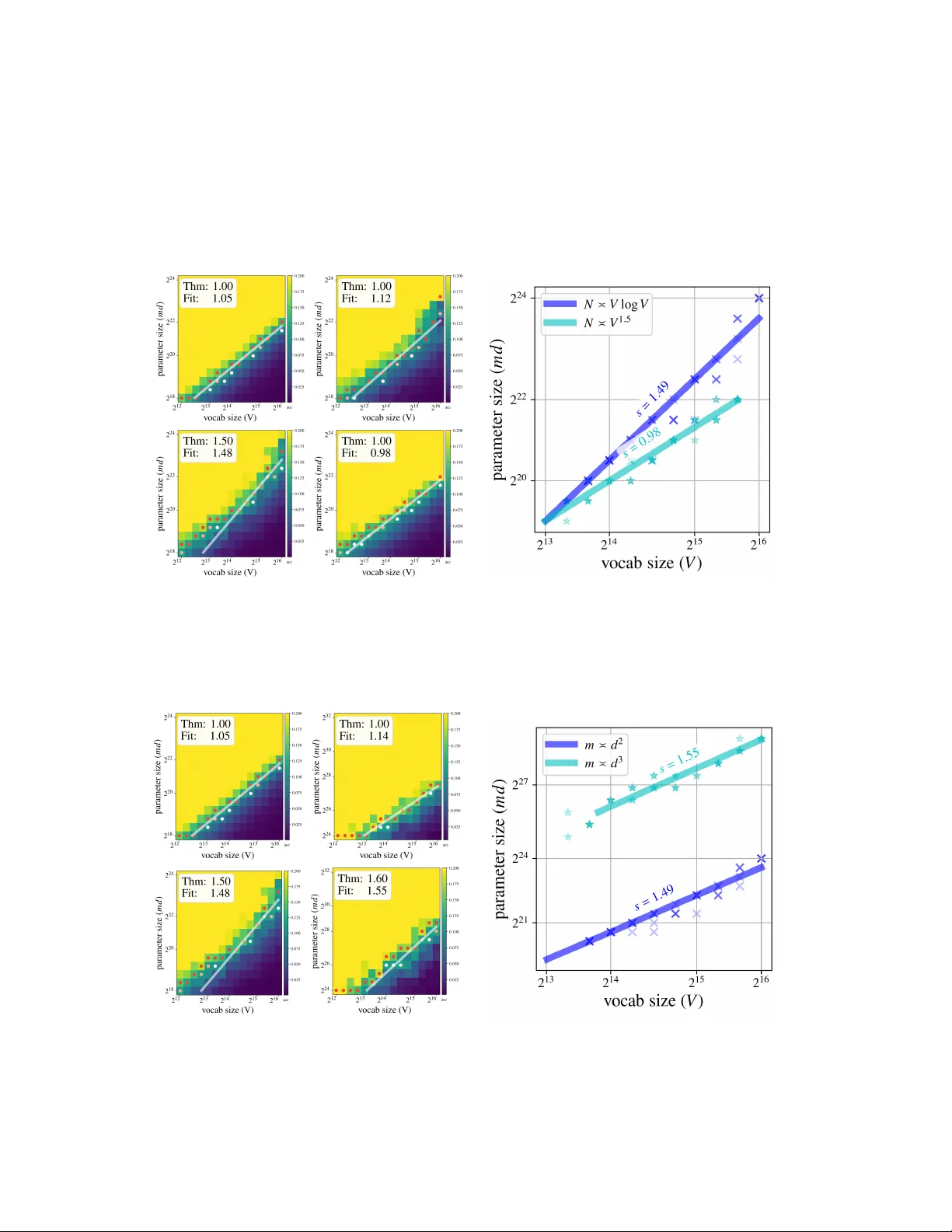
Learning to Recall with T ransformers Bey ond Orthogonal Em b eddings Nuri Mert V ural ∗ , Alb erto Bietti † , Mahdi Soltanolk otabi ‡ , Denn y W u § Marc h 18, 2026 Abstract Mo dern large language mo dels (LLMs) excel at tasks that require storing and retrieving knowledge, suc h as factual recall and question answering. T ransformers are central to this capabilit y b ecause they can enco de information during training and retrieve it at inference. Existing theoretical analyses t yp- ically study transformers under idealized assumptions such as inﬁnite data or orthogonal embeddings. In realistic settings, how ever, mo dels are trained on ﬁnite datasets with non-orthogonal (random) em- b eddings. W e address this gap by analyzing a single-lay er transformer with random em b eddings trained with (empirical) gradient descent on a simple token-retriev al task, where the mo del must identify an informativ e token within a length- L sequence and learn a one-to-one mapping from tokens to labels. Our analysis trac ks the “early phase” of gradient descen t and yields explicit formulas for the mo del’s storage capacit y—revealing a m ultiplicative dep endence b et ween sample size N , embedding dimension d , and sequence length L . W e v alidate these scalings numerically and further complement them with a low er b ound for the underlying statistical problem, demonstrating that this multiplicativ e scaling is intrinsic under non-orthogonal embeddings. Code to repro duce all experiments is publicly a v ailable. 1 1 In tro duction Large language mo dels (LLMs) routinely answ er kno wledge questions with little or no external context, indicating that substan tial factual information is stored in parameters and can b e retriev ed by suitable prompts [ PRL + 19 , JXAN20 , RRS20 ]. A deep er theoretical understanding of how such parametric memories are learned and accessed is increasingly imp ortan t: it can guide scaling choices (e.g., trading oﬀ memory capacit y against compute budgets, [ CIJ + 22 , AZL24 ]) and clarify failure modes (e.g., hallucination, [ ZBC + 25 , HZG + 25 ]). Motiv ated by empirical results do cumen ting the prev alence of parametric factual recall and its scaling with model size [ AZL24 , MSG + 25 ], recent theoretical w orks hav e begun to analyze the capacity and learning dynamics of transformers on controlled factual-recall tasks [ CDB24 , NLB25 ]. Man y theoretical studies of transformer optimization work in p opulation-dynamics settings and adopt simplifying assumptions, such as treating token em b eddings as orthogonal or one-hot vectors (see, e.g., [ TWZ + 23 , CSWY24 , GHR24 ]). While these choices do not alwa ys reﬂect practical applications, they mak e the mathematics, particularly gradient calculations, more tractable, and population analyses of this kind do not characterize the statistical or computational complexity of gradien t-based learning. In factual-recall setups, strictly orthogonal embeddings are known not to b e capacit y-optimal, whereas random or non- orthogonal embeddings (i.e., sup erp osition ) enable near-optimal factual storage [ NLB25 ]. At the same time, remo ving the orthogonality assumption in tro duces token in terference that leads to intricate optimization b e- ha vior (e.g., oscillatory tra jectories [ CSB24 ]), and in practice, superp osition-based, memory-eﬃcien t solutions ∗ Universit y of T oron to and V ector Institute. vural@cs.toronto.edu . W ork done while in terning at the Flatiron Institute. † Flatiron Institute. abietti@flatironinstitute.org . ‡ Universit y of Southern California. soltanol@usc.edu . § New Y ork Univ ersity and Flatiron Institute. dennywu@nyu.edu . 1 Code av ailable at https://github.com/nurimertvural/learning- to- recall- experiments . 1 can also b e more diﬃcult to train [ EHO + 22 ], whic h highligh t a fundamental trade-oﬀ betw een optimization and statistical eﬃciency v ersus storage capacit y . Motiv ated by the abov e gaps, w e aim to address the follo wing question. Can we char acterize the optimization and sample c omplexity of a tr ansformer with non-ortho gonal emb e ddings tr aine d by gr adient desc ent in the le arning of a factual r e c al l task? 1.1 Our Contributions In this paper, we analyze gradien t-based learning of a single-la yer transformer with an atten tion+MLP block and random embeddings on a synthetic task inspired by [ NLB25 ]: the mo del m ust retrieve an informativ e tok en from a context containing man y noisy tokens via attention, then map it to the correct lab el via factual recall. T o mitigate the complex optimization dynamics arising from non-orthogonal em b eddings, we follow [ BCB + 23 , ORST23 ] and consider a simpliﬁed training regime in volving only a few gradien t steps with ﬁnite samples on the atten tion and v alue matrices. This p erspective eﬀectively zo oms in the “early phase” of the training as commonly studied in the feature-learning literature [ BES + 22 , DLS22 , DKL + 23 , VE24 , WNB + 25 ]. Our analysis provides a ﬁne-grained characterization of how vocabulary size V , sample size N , em b edding dimension d , sequence length L , and MLP width m interact to p ermit successful gradien t-based learning of the recall mec hanism. Our main result states that • The success of learning dep ends on ( V , N , d, L, m ) in a multiplic ative manner: learning b ecomes easier as ( N , d, m ) increase, whic h reﬂects the beneﬁts of more data, higher-dimensional (and th us more orthogonal) em b eddings, and larger MLP width; whereas learning b ecomes harder as ( V , L ) increase; that is, the task b ecomes more diﬃcult with a larger v o cabulary or longer sequences. This multiplicativ e relation is visualized in Figure 1a , where we examine ho w the parameter size m × d depends on the vocabulary size V for diﬀerent sequence lengths L . The full phase diagram corresp onding to this relation, whic h formalizes Figure 1a , is sho wn in Figure 1b . • Consequently , while optimal capacit y and sample complexity can b e ac hieved join tly for short sequences, successful learning on long sequences requires either a larger embedding dimension (thus sacriﬁcing capac- it y) or larger sample sizes (w orsening statistical complexity). The m ultiplicative rate ab o v e formalizes the “tradeoﬀ ” in tuition that smaller embedding dimension d — whic h increases sup erposition and thereby improv es storage capacity — simultaneously yields a harder learning problem, as reﬂected in the required sample size. W e complemen t this with a statistical lo wer bound sho wing that the trade-oﬀ is inheren t for any estimator that accesses only gradien t information from the initialized transformer. Finally , although our theory is deriv ed for a speciﬁc three-step training algorithm, w e empirically observ e qualitatively similar m ultiplicative scaling when the transformer is optimized b y gradient descen t to low empirical risk. 1.2 Related W ork Learning dynamics of transformers. A growing line of work analyzes how transformers acquire sp e- ciﬁc b eha viors from gradien t-based training. Much of this literature imp oses p opulation-lev el assumptions and orthogonal/one-hot embeddings to make gradients tractable, often on discrete synthetic tasks [ LLR23 , BCB + 23 , TWCD23 , NDL24 , CSWY24 , GHR24 , CBB25 , WNB + 25 ]. Several works study few-step training regimes as a lens on the “early phase” of feature learning [ BCB + 23 , WNB + 25 ]. Beyond discrete settings, related analyses inv estigate attention learning for con tin uous inputs and sparse-signal retriev al [ ORST23 , MBBB25 , DMB + 26 ]. A complemen tary thread fo cuses on the eme rgence of in-context learning and induc- tion mec hanisms: single- and t wo-la y er atten tion trained on linear-regression or Mark ov data pro v ably imple- men ts gradien t-descent-lik e up dates and generalized induction heads [ V ONR + 23 , ZFB24 , CSWY24 , NDL24 ]. These results typically rely on simpliﬁed settings and do not address storage capacit y . In contrast, our work analyzes ﬁnite-sample training with non-orthogonal embeddings in an attention+MLP arc hitecture with a particular focus on factual recall. 2 (a) No Learning ( md ≪ V ) vocab size ( V ) width ( m ) Slope ≍ d Slope ≍ 1 /d Mean Bias md ≳ mL 4 3 V 2 3 N 2 3 Gradien t Noise md ≳ mL 1 4 √ N MLP Noise md ≳ V √ mL 2 N dL d 2 L (b) Figure 1: (a) Empirical scaling of the parameter size required for a GD-trained one-lay er transformer to learn factual recall, where we use m ≍ d 2 (see Section 4.2 for details). F or small L , the trained model achiev es the optimal capacit y V ≍ md (purple line). As the sequence length L increases, the scaling c hanges, suggesting a multiplicativ e rate (blue and red lines). (b) Phase diagram for the theoretical scaling of the parameter coun t given in Corollary 2 . Each region corresp onds to a regime where a particular noise term in Theorem 1 is dominan t. The parameter-size condition ( md ) in each region is given in Corollary 2 . Asso ciativ e memories and storage capacity . Classical asso ciativ e memories (Hopﬁeld-t yp e mo dels) study recall of v ector patterns and established foundational capacit y results [ Hop82 , AGS85 , MPR V88 , KH16 , DHL + 17 , RSL + 20 , SIS21 ]. Recen t works adapt asso ciativ e-memory viewp oin ts to transformers, mo deling inner w eights as superp ositions of outer products and deriving scaling la ws and optimization b eha v- iors [ BCB + 23 , CDB24 , CSB24 ]. In factual recall sp eciﬁcally , random (non-orthogonal) embeddings enable near-parameter-coun t storage, whereas strictly orthogonal em b eddings are not capacit y-optimal [ NLB25 ]. V arious empirical works ha ve studied the mechanisms and scaling b eha viors of LLMs in factual asso ciation tasks [ PRL + 19 , JXAN20 , GSBL20 , AZL24 ]. W e pro vide a theoretical analysis of such mechanisms and quan tify how vocabulary size, sequence length, embedding dimension, and MLP width jointly gov ern learn- ing eﬃciency . Our work op erates in a setting similar to [ NLB25 ] but allows ﬁnite samples and explicitly considers gradient descent dynamics. Our result is similar to the ﬁnite-sample results in [ ORST23 ], where the required sample size gro ws with the dimensionalit y and sparsit y level of informativ e tokens, while w e allo w non-orthogonal embeddings and sho w optimal capacity as in [ NLB25 ] under certain conditions. 2 Problem Setting Our goal is to understand the capacit y of transformers trained on ﬁnite data with non-orthogonal embeddings, in a setting where the relev ant information is hidden in a p oten tially large sequence of non-informative noisy tok ens. The attention op eration should then identify the relev ant token, while the subsequent linear or MLP blo c k can then recall the correct lab el via an asso ciativ e memory mechanism. This is similar to the factual recall task studied b y [ NLB25 ], with simpliﬁcations that mak e the analysis more tractable, as detailed below. Notation. σ denotes the softmax function. 1 V : = (1 , . . . , 1) ⊤ ∈ R V is the V -dimensional all-ones vector; e i is the one-hot vector with a 1 in the i -th position (dimension understo o d from con text). W e use ≳ (resp. ≲ ) to mean “ ≥ ” (resp. “ ≤ ”) up to p olylogarithmic factors in V : f V ≳ g V ⇐ ⇒ f V ≥ p oly(log V ) g V and f V ≲ g V ⇐ ⇒ f V ≤ poly(log V ) g V , for some ﬁxed p olynomial. Lastly , ∥·∥ 2 denotes the Euclidean norm for v ectors and the op erator (sp ectral) norm for matrices. Problem setup. Let the input/output tokens take v alues from a ﬁnite alphabet [ V ] : = { 1 , · · · , V } . F or notational conv enience, we represen t the alphab et by the one-hot vocabulary V = { e 1 , · · · , e V } . Eac h example in the data consists of a length- L input sequence X = [ x 1 , . . . , x L ] ∈ V L and a lab el p ∈ V generated as follo ws: 3 • Input tok ens are sampled indep enden tly and uniformly: [ x 1 , . . . , x L ] ∼ Unif ( V L ). • Informative p osition is a random index ℓ ∼ Unif ([ L ]) independent of X . • Gr ound-truth function is a p erm utation matrix Π ∗ ∈ { 0 , 1 } V × V . Lab els are generated as the p erm uted informativ e token, p = Π ∗ x ℓ , while the remaining tokens are non-informative. The goal is to identify the correct token position ℓ and learn the target function (permutation) Π ∗ . T ransformer architecture. W e consider a basic transformer blo c k which ﬁrst maps input tokens into a d - dimensional embedding space where d < V . The embedding la yer is parameterized b y ( Z in , Z out , z trig , z EOS ) ∈ R d × V × R d × V × R d × R d , where • The input tok ens are embedded b y the columns of the matrix Z in ∈ R d × V . • Output tok ens are asso ciated with unembedding vectors, which are collected in Z out ∈ R d × V . • z trig is a trigger v ector that marks the informativ e tok en. • z EOS is the special embedding vector that marks the end-of-sequence. Giv en the em b edding parameters, we deﬁne the self-atten tion head, parameterized by the key-query matrix W KQ ∈ R d × d , whic h op erates on the embedded sequence of inputs Z in X ∈ R d × L : attn( X ; W KQ ) : = Z in X σ  ( z trig e ⊤ ℓ + Z in X ) ⊤ W KQ z EOS  . (2.1) The trigger embedding z trig is used to “mark” the informativ e token with a special direction, mimic king the b eha vior of previous transformer lay ers that ma y learn to ﬂag particular tok ens by adding to its residual stream 2 (note that the num b er of trainable parameters inside softmax can b e reduced to d b y collapsing W KQ z EOS in to a vector). W e consider tw o diﬀeren t learning models: an A ttention-only model and a width- m , t wo-la y er neural netw ork model Attention-MLP , deﬁned as: ˆ p ( X ; V , W KQ ) =    σ  Z ⊤ out V attn( X ; W KQ )  , A ttention only σ  Z ⊤ out V ϕ ( W in attn( X ; W KQ )  , Atten tion-MLP (2.2) where V ∈ R d × d for the Attention-only and V ∈ R d × m , W in ∈ R m × d for the Attention-MLP mo del. Note that compared with A ttention-only mo del, the Attention-MLP mo del contains an additional set of trainable parameters and nonlinear activ ation function ϕ b efore the v alue matrix. Similar to in [ NLB25 ], the MLP allo ws using a smaller em b edding dimension d while keeping the capacit y large b y increasing width m . F or the Attention-MLP , we k eep W in ﬁxed at its random initialization. The trainable parameters for b oth of our models are ( V , W KQ ). W e use cross-entrop y loss to train our mo del: L  ( V , W KQ ) , ( X , p )  = − P V i =1 p i log ˆ p i . T raining algorithm. F ollowing [ ORST23 ], we consider a 3-step gradien t-based algorithm with dataset { ( X i , p i ) } N i =1 with a sample size of N . W e initialize our parameters as V (0) = 0, W (0) KQ = 0 and use the learning rates η , γ > 0: V (1) = V (0) − η · 1 N P N i =1 ∇ V L  ( V (0) , W (0) KQ ); ( X i , p i )  (2.3) W (1) KQ = W (0) KQ − γ · 1 N P N i =1 ∇ W KQ L  ( V (1) , W (0) KQ ); ( X i , p i )  (2.4) V (2) = V (1) − γ · 1 N P N i =1 ∇ V L  ( V (1) , W (1) KQ ); ( X i , p i )  . (2.5) 2 The “trigger” terminology is b orro wed from [ BCB + 23 ], where a sp ecial previous token “triggers” a retriev al operation in the context of induction heads. Our setup resembles learning only the “induction head” la yer assuming the ﬁrst “previous tok en head” la yer is already in place. The triggers often app ear to be single directions in interpretabilit y literature, see, e.g., the “X in opposite of X” feature in [ KAK + 25 ]. 4 Net work prediction and storage. Given our mo del and training metho d, we use argmax deco ding at inference and deﬁne the test accuracy as Accuracy : = P ( X , p )  p = e pred( X )  , where pred( X ) : = arg max j ∈ [ V ] ˆ p j ( X ; V (2) , W (1) KQ ) , where ˆ p ( X ; V (2) , W (1) KQ ) is the netw ork output deﬁned in ( 2.2 ). In what follo ws, we c haracterize conditions under which the mo del stores the informative tokens asymptotically , i.e., Accuracy → 1 as V → ∞ , in terms of the relev ant parameters ( V , N , d, L, m ). 3 Main Results W e ﬁrst present our general theorem on learnability via gradient descent, and then sp ecialize into diﬀerent regimes to derive more interpretable scaling b eha viors in Section 4 . W e pro vide a proof sketc h in Section 5 , and defer the full pro of to Appendix C . 3.1 T echnical Assumptions W e ﬁrst state generic assumptions that apply to b oth the A ttention-only and A ttention-MLP mo dels. Assumption 1. • Par ameter r ange: L et L = V c for c ∈ (0 , 1) , Ω( V log V ) ≤ N = o ( V L ) , and V ≥ Ω(1) . • L e arning r ate: We use a suﬃciently smal l le arning r ate η for the initial step ( 2.3 ) , and suﬃciently lar ge le arning r ate γ for the r emaining steps ( 2.4 ) - ( 2.5 ) that satisfy Assumption 4 . • Emb e ddings: L et Z in , Z out ∈ R d × V b e indep endent Gaussian matric es, and let z trig , z EOS ∈ R d b e indep endent Gaussian ve ctors, al l with i.i.d. entries distribute d as N (0 , 1 / d ) . W e assume c ∈ (0 , 1) since in many practical pretraining setups, the con text length is smaller than the v o cabulary size, and the condition L ≪ V simpliﬁes several terms in the pro ofs. The low er bound N ≳ V log V is required so that eac h elemen t from the alphabet of size V is seen at least once with high probabilit y . The learning rates follow prior analyses [ ORST23 , NDL24 ]: a small η ensures that the netw ork’s predictions remain close to uniform after the ﬁrst step, whereas a large γ is needed to push the attention scores and predictions to ward one-hot vectors. In addition to the abov e assumptions, we require the transformer mo del to hav e suﬃcien t capacity to reach p erfect test accuracy . Such conditions are c haracterized by [ NLB25 ]. F or the Attention-only mo del, we hav e the follo wing condition (see [ NLB25 , Theorem 3]). Assumption 2 (Atten tion-only) . F or the Atten tion-only mo del, we r e quir e d 2 ≳ V . With a nonlinear MLP lay er, a smaller em b edding dimension can suﬃce if the width is large enough. Hence for A ttention-MLP we require the following condition. Assumption 3 (Atten tion-MLP) . F or the Atten tion-MLP mo del, we assume that • Polynomial activation: ϕ : R → R satisﬁes ϕ (0) , ϕ ′ (0) , ϕ ′′ (0)  = 0 . • MLP width: md ≳ V and d ≳ V 1 k ⋆ +1 , wher e k ⋆ denotes the smal lest nonzer o Hermite mo de of ϕ , i.e., k ⋆ : = min { k > 0 : E Z ∼N (0 , 1) [ ϕ ( Z ) h k ( Z )]  = 0 } wher e h k is the k th Hermite p olynomial. • Initialization: W in ∈ R m × d ar e ﬁxe d with entries i.i.d. distribute d as N (0 , 1) . The nonlinear MLP la yer allows us to comp ensate for the em b edding dimension and go beyond the d 2 ≳ V lo wer b ound required by the A ttention-only mo del (Assumption 2 ). Note that md ≳ V is a necessary condi- tion for capacity as shown in [ NLB25 ]. The additional requirements imp osed on the p olynomial activ ation function appear to b e artifacts of our three-step GD analysis, and w e conjecture that they could b e relaxed when considering a longer training horizon. 5 3.2 Learnabilit y Statement No w we are ready to present our main theorem on the complexity of learning the factual recall task. Sp eciﬁ- cally , the transformer learns the desired mechanism when the signal term dominates the noise and bias terms as stated below. Theorem 1. L et Assumptions 1 and 3 hold for A ttention-MLP , and 1 and 2 hold for A ttention-only . The A ttention-MLP mo del achieves Accuracy = 1 − o V (1) with pr ob ability 1 − o V (1) whenever 1 V L 2 | {z } Signal ≳ 1 N √ Ld ( d ∧ L ) | {z } Gr adient noise + 1 N √ V d ( d ∧ L ) | {z } Me an bias + 1 N d √ m | {z } MLP noise . (3.1) F or the Atten tion-only mo del, the same holds with the last MLP noise term r emove d. Theorem 1 characterizes learnability as a function of ( V , N , d, L, m ) and identiﬁes the following terms that impact the gradien t signal-to-noise ratio: 1. Signal measures the alignmen t b et ween the key–query weigh ts W (1) KQ and the trigger z trig . 2. Gr adient noise is due to the concentration error in the up date of W (1) KQ . 3. Me an bias arises from the nonzero mean of token vectors { X i } N i =1 . 4. MLP noise reﬂects the randomness in the MLP w eight matrix W in in A ttention–MLP . W e make the following observ ations. • Multiplicativ e scaling. Note that the parameters ( V , N , d, L, m ) interact in a m ultiplicativ e fashion. F or example, the noise and bias terms in ( 3.1 ) all decay with ( N × d ), suggesting that increasing the em b edding dimensions d can lo wer the statistical complexit y of learning the correct recall mec hanism. While the full 5-parameter trade-oﬀ can b e opaque, in Section 4 we fo cus on sp eciﬁc regimes that lead to simpliﬁcation of the scaling relationship and v alidate the rate empirically . • Optimal storage & sample complexity . Recall that the capacit y-optimal construction for the factual recall task requires md ≳ V parameters (or d 2 ≳ V for Attention–only ); and as discussed earlier, a sample size N ≍ V log V is necessary to observe all distinct tok ens. ( 3.1 ) implies that in the small- L regime, the optimized transformer achiev e optimal capacit y and sample complexity simultaneously . F or longer sequences, ho wev er, these t wo conditions ma y not b e achiev ed at the same time, i.e., one must increase either the netw ork width or sample size b ey ond optimality to learn the task — this conﬁrms the empirical observ ation in Figure 1 . 3.3 Statistical Low er Bound Theorem 1 provides an upper b ound (i.e., suﬃcien t condition) on the model and sample size for learning factual recall under a 3-gradien t-step optimization pro cedure. W e complement this suﬃcien t condition with a low er b ound indicating that the multiplicativ e dep endence on the problem parameters is partly statistical; that is, the scaling b eha vior will b e observed in an y mo del satisfying the broader conditions stated b elow. Our low er b ound applies to statistical metho ds that can query the dataset through the attention outputs at initialization, h i : = attn( X i , W (0) KQ ). In particular, we consider queries of the form h i as the gradient with resp ect to the key–query matrix W KQ dep ends on { h i , h i h ⊤ i } N i =1 (see ( B.1 )). The statemen t is given b elo w: Theorem 2 (Informal) . A ny metho d that r elies on the noisy version of the queries { h i , h i h ⊤ i } N i =1 fails, i.e., Accuracy → 1 with ﬁnite pr ob ability, if N ≲ V min { 1 , L/d 2 } . The complete statement of Theorem 2 is deferred to Theorem 4 in App endix E . W e observe that the low er b ound does not exactly matc h our upper bound in Theorem 1 , as Signal ≲ Gr adient Noise in ( 3.1 ) is stronger than the stated low er bound. This being said, Theorem 2 also conﬁrms the multiplicativ e scaling, hence 6 (a) N ≍ V log V (b) N ≍ V 1 . 5 (c) Atten tion only , L ≍ V Figure 2: Empirical scaling of parameter size via three-step GD for the A ttention-only model. In (a) and (b), top-left and top-righ t use L ≍ V 0 . 5 ; bottom-left and b ottom-righ t use L ≍ V . In (c), w e compare the parameter coun ts from (a) and (b) for the L ≍ V case under tw o sample-size regimes, N ≍ V log V and N ≍ V 1 . 5 . Line ﬁtting: W e identify in the heatmaps the smallest embedding dimension that achiev es accuracies { 0 . 1 , 0 . 125 , 0 . 15 } and perform a least squares ﬁt. The slopes of the ﬁtted lines and their theoretical counterparts are rep orted on the heatmaps. suggesting the trade-oﬀ b et ween capacity and sample eﬃciency is present in a boarder class of learning algorithms. A stronger computational low er b ound for transformers and gradient-based optimization is an in teresting problem we leav e for future w ork. 4 Implications and Empirical V eriﬁcations In this section, we leverage our main theorem to obtain more concrete scalings b etw een parameters, and presen t empirical evidence on the deriv ed multiplicativ e rate. 4.1 A tten tion-only Mo del W e start with the A ttention-only mo del which gives a simpler phase diagram. Corollary 1. F or the A ttention-only mo del, the b ottlene ck term in ( 3.1 ) is the Mean bias term. Ther efor e, The or em 1 is e quivalent to the p ar ameter size r e quir ement d 2 ≳ max { V , V 2 / 3 L 8 / 3 / N 4 / 3 } . W e make the following observ ations: • The condition in Corollary 1 is the maximum of t wo terms, where d 2 ≳ V is due to the capacit y require- men t in Assumption 2 , whereas the second term ensures Signal ≳ Me an bias and implies a multiplicativ e scaling b et ween the sample size N and embedding dimension d (i.e., increasing one of the parameters can comp ensate for the other). • Note that the Me an bias term arises from a nonzero token mean, which can p oten tially b e alleviated by cen tering the tok ens, for instance through an appropriate normalization lay er. Exploring the eﬀect of applying normalization in this mo del is an in teresting direction for future w ork. Empirical Findings. W e run the three-step gradient descent algorithm on an Attention-only mo del ov er v arying V and d , and rep ort the accuracies in the heatmaps (Figure 2 ). The plots are in log-log scale; therefore, the slop es give the exp onen t s in d ≍ V s . As shown in the top row of Figures 2a - 2b , the slope for relativ ely small L (where L ≍ V 0 . 5 ) matc hes the optimal capacity condition d 2 ≍ V . By contrast, when the 7 con text windo w is larger ( L ≍ V ), the requiremen t becomes d ≍ V , whic h is also reﬂected in the exp erimen tal results, as observ ed in the bottom panel of Figure 2a . In Figure 2b we run exp erimen ts with increasing sample size to observ e the multiplicativ e trade-oﬀ. As seen in the b ottom ﬁgure of Figure 2b , increasing the sample size from V log V to V 1 . 5 reduces the exp onen t of the parameter size from 2 . 02 to 1 . 42 (the theoretical v alue is s = 1 . 32). Finally , the learnability thresholds for L ≍ V in Figures 2a and 2b are plotted together in Figure 2c , to illustrate that increasing the sample size can compensate for the num b er of parameters in the netw ork. (a) N ≍ V log V (b) N ≍ V 1 . 5 (c) L ≍ V 0 . 5 and m ≍ d 2 Figure 3: Empirical scaling of parameter size for the Attention-MLP mo del under tw o sample size regimes, N ≍ V log V and N ≍ V 1 . 5 . In (a) and (b), top-ro w uses L ≍ V 0 . 25 ; b ottom-ro w uses L ≍ V 0 . 5 . In (c), w e compare the parameter counts from (a) and (b) for the L ≍ V 0 . 5 case under b oth sample-size regimes. (a) m ≍ d 2 (b) m ≍ d 3 (c) L ≍ V 0 . 5 and N ≍ V log V Figure 4: Empirical scaling of embedding parameter size for the Attention-MLP mo del under tw o width regimes, m ≍ d 2 and m ≍ d 3 . In (a) and (b), top-row uses L ≍ V 0 . 25 ; b ottom-ro w uses L ≍ V 0 . 5 . In (c), we compare the parameter counts from (a) and (b) for the L ≍ V 0 . 5 case under b oth width regimes. 8 4.2 A tten tion-MLP Mo del F or the attention-MLP mo del, the nonlinear MLP lay er in tro duces additional phases as stated b elow. Corollary 2. F or the A ttention-MLP mo del, The or em 1 tr anslates to md ≳ V and Signal ≳      MLP noise , m = o ( d 2 L ) and m = o ( dV ) Gradien t noise , V ≳ dL and m ≳ d 2 L Mean bias , V = o ( dL ) and m ≳ dV , wher e • Signal ≳ MLP noise is e quivalent to md ≳ V √ mL 2 N . • Signal ≳ Gradien t noise is e quivalent to md ≳ V mL 1 4 √ N • Signal ≳ Mean bias is e quivalent to md ≳ mL 4 3 V 1 3 N 2 3 . The phase diagram for the A ttention-MLP mo del is visualized in Figure 1b . Compared to the Attention- only case, it exhibits additional regimes b ecause we can trade oﬀ m and d and thus use a smaller embedding dimension; this can lead to diﬀerent dominan t terms in the gradient. In particular, since large L and d en tail a larger magnitude of the Me an bias (as in the Attention-only setting), increasing the MLP width m and thereb y reducing the required em b edding dimension d ma y suppress this bias term. Empirical Findings. W e run the 3-step gradient descent algorithm on an Atten tion-MLP netw ork ov er v arying V and d and plot the accuracies in Figures 3 and 4 . W e take the nonlinearit y to b e the mixture of t wo Hermite polynomials ϕ = 0 . 7 h 2 + 0 . 3 h 3 , satisfying the conditions in Assumption 3 . W e run exp erimen ts with width m ≍ d 2 and m ≍ d 3 . Due to the prohibitiv e cost of increasing the width further, we restrict ourselv es to the MLP noise -dominated region. In Figure 1a , we plot the scaling of the num b er of parameters ( md ) as a function of vocabulary size V for diﬀeren t sequence-length regimes in L . W e observe that L ≍ V 0 . 25 requires md ≍ V , which is the optimal capacit y , as predicted by our theory . As L increases, we need more parameters to achiev e the same capacity , as observed in the L ≍ V 0 . 5 and L ≍ V 0 . 75 cases in Figure 1 , where the slop es agree with our theoretical predictions as w ell (see also Figures 3a and 3b ). W e further test the eﬀect of sample size in Figure 3 , where we use L ≍ V 0 . 5 and m ≍ d 2 . W e plot b oth heat maps in Figures 3a and 3b , and the ﬁtted lines for L ≍ V 0 . 5 together in Figure 3c . W e observe that increasing N from N ≍ V log V to N ≍ V 1 . 5 reduces the netw ork size to the optimal lev el, aligning with our theoretical prediction. The heatmap v ersions of these exp erimen ts are sho wn in Figures 3a and 3b . Lastly , we probe the width scaling b y keeping the sample size N ≍ V log V and L ≍ V 0 . 5 ﬁxed in Figure 4 . Here, we observe that we can reduce the embedding-dimension requirement b y increasing m in Theorem 1 , although it increases the total parameter count ov erall, as seen in Figures 4b and 4c , since width m ust gro w prop ortionally more than d to ac hieve the same accuracy . This is also consisten t with our result. 4.3 Bey ond Early Phase of T raining While our theoretical analysis fo cuses on a particular three-gradient-step training pro cedure, we empirically observ e qualitatively similar multiplicativ e scalings when the transformer mo del is optimized b ey ond the “early phase”. Speciﬁcally , we train our A ttention-only mo del using Adam [ KB15 ] with mini-batch gradients. In the exp erimen ts, w e use la yer normalization in b oth the attention and output la yers and set the learning rate to 0 . 005. W e use a batch size of ⌊ N / 2 ⌋ (except in the last exp eriment, where we use ⌊ N / 16 ⌋ ), and run the training for 16 ep o c hs. W e highligh t the following observ ations: • Cap acity impr ovement with multi-p ass tr aining. In the top ro w of Figure 5 , we plot the heatmaps for L ≍ V and N ≍ V log V . In early training the slop e is sub optimal; notably , b y the end of Ep och 1 it closely aligns with our theoretical prediction. Moreov er, training the net work additional ep ochs impro ves the capacit y condition to a near-optimal lev el, as sho wn in Figures 5c and 5d . 9 • Eﬀe ct of sample size. In the b ottom ro w of Figure 5 , w e plot the heatmaps for L ≍ V and N ≍ V 1 . 5 . W e observ e a similar tra jectory in capacity , while the ov erall capacities improv e compared to the small-sample regime, sho wing the multiplicativ e dep endence on sample size N . • Eﬀe ct of se quenc e length. In Figure 6 , w e plot the heatmaps for L ≍ V 0 . 85 and N ≍ V log V . W e observe impro vemen ts in capacity o ver m ultiple ep o c hs, while the capacity is larger than in the L ≍ V setting at ev ery stage of training, whic h shows the eﬀect of the sequence length L . • Eﬀe ct of b atch size. In Figure 7 , we rep eat the exp erimen ts from this section using the same learning rate and architecture but with a smaller batc h size ⌊ N / 16 ⌋ . As b efore, we consider L ≍ V in t wo sample-size regimes, N ≍ V log V and N ≍ V 1 . 5 . W e observ e b eha vior similar to the larger batch size setting, but with improv ed slop es in Figure 7 . This suggests that smaller batch sizes ma y improv e capacity in practice. Ov erall, these experiments suggest that the m ultiplicativ e relation betw een the h yp erparameters remains throughout training. How ev er, the exp onen ts dep end on the iteration n umber and batc h size. Understanding ho w capacity evolv es during training remains an in teresting op en question. (a) Ep och 1 (b) Ep och 2 (c) Ep och 8 (d) Ep och 16 (e) Ep och 1 (f ) Ep och 2 (g) Ep och 8 (h) Ep och 16 Figure 5: Empirical scaling of the parameter size for the Attention-only mo del under t wo sample size regimes. T op r ow (a–d): N ≍ V log V . Bottom r ow (e–h): N ≍ V 1 . 5 . The model uses L ≍ V and is trained using Adam ov er 16 ep ochs. W e observ e that the capacity impro ves as the num ber of ep ochs increases. (a) Ep och = 1 (b) Ep och = 2 (c) Ep och = 8 (d) Ep och = 16 Figure 6: Empirical scaling of the parameter size for the Attention-only model with N ≍ V log V and L ≍ V 0 . 85 . The mo del is trained using Adam o ver 16 ep o c hs. The slopes are smaller than in Figure 5 , which is consistent with the shorter sequence length. 10 (a) Ep och 1 (b) Ep och 2 (c) Ep och 8 (d) Ep och 16 (e) Ep och 1 (f ) Ep och 2 (g) Ep och 8 (h) Ep och 16 Figure 7: Empirical scaling of the parameter size for the Attention-only mo del ( L ≍ V ), trained with Adam using a batc h size of ⌊ N / 16 ⌋ . T op r ow (a–d): N ≍ V log V . Bottom row (e–h): N ≍ V 1 . 5 . 5 Pro of Ov erview In this section, we outline the main ideas b ehind the pro of of Theorem 1 . The key observ ation is that the recall task is achiev ed with near-p erfect accuracy if and only if the attention mec hanism can distinguish informativ e tokens. Once this o ccurs, the remaining task reduces to learning a linearly separable problem, whic h is well understo od. Therefore, the proof fo cuses on the attention scores in ( 2.1 ) and characterizes the conditions under whic h the mec hanism selects the informative tokens. The pre-softmax scores ev aluated on a fresh sequence X in , with the k ey-query matrix given b y the ﬁrst gradien t-descent iterate W (1) KQ , are giv en by scores : =  z trig e ⊤ ℓ + Z in X in  ⊤ W (1) KQ z EOS . (5.1) By substituting the exact expression for W (1) KQ in to ( 5.1 ), we analyze scores. F or intuition, we present the simpliﬁed expression below (see ( B.1 ) for the full expression): scores ≈ γ ∥ z trig ∥ 2 2 e ℓ  1 N L N X i =1 x ⊤ i,ℓ Z ⊤ in ( V (1) ) ⊤ Z out ( p i − 1 V 1 V )  | {z } Informative (5.2) + γ X ⊤ in Z ⊤ in  1 N L N X i =1 Z in X i X ⊤ i Z ⊤ in ( V (1) ) ⊤ Z out ( p i − 1 V 1 V )  | {z } Non-informative . (5.3) Here V (1) denotes the ﬁrst iterate of the v alue matrix deﬁned in ( 2.3 ). The informative term in ( 5.2 ) captures the alignmen t b et ween the trigger v ector in the fresh input and the one encoded in the learned w eights W (1) KQ , and therefore con tains p osition information ab out the informative token. By contrast, the non-informative term in ( 5.3 ) reﬂects correlations b et ween tok ens and do es not con tain information ab out the tok en p osition. Th us, the pro of reduces to c haracterizing the conditions under whic h the informativ e term in ( 5.2 ) dominates the non-informativ e term in ( 5.3 ). Under these conditions, the attention mechanism correctly iden tiﬁes the informativ e token, and the remaining prediction problem b ecomes linearly separable. 11 5.1 Empirical Dynamics with Non-Orthogonal Embeddings W e no w pro vide a proof sk etch for the ﬁnite-sample setting with non-orthogonal em b eddings and explain ho w eac h noise term in Theorem 1 arises. In particular, we consider ( 5.2 )–( 5.3 ) and, without loss of generality , assume ℓ = 1 and Π ∗ = I V (accordingly , p i = x i, 1 ). Our goal is to show ho w the Signal , Gr adient noise , Me an bias , and MLP noise terms arise from the dynamics of the ﬁrst gradient step. The analysis pro ceeds in tw o steps. First, we sho w that the ﬁrst iterate of the v alue matrix V (1) admits a natural decomposition into mean, bias, and noise comp onen ts. W e then sho w how this decomp osition giv es rise to the terms app earing in Theorem 1 . 5.1.1 Decomposition of the v alue matrix Both the informativ e and non-informativ e terms dep end on V (1) . W e show that it can b e decomposed as V (1) = Z out  1 N L N X i =1 ( x i, 1 − 1 V 1 V )( X i 1 L ) ⊤  Z ⊤ in (5.4) = Z out  1 V L ( I V − 1 V 1 V 1 ⊤ V ) | {z } Mean + 1 V N N X i =1 ( x i, 1 − 1 V 1 V ) 1 ⊤ V | {z } Bias + 1 √ LV N Ξ | {z } Noise  Z ⊤ in (5.5) where the noise term is given by Ξ : = r V LN  N X i =1 ( x i, 1 − 1 V 1 V )( X i 1 L − L V 1 V ) ⊤ − 1 V ( I V − 1 V 1 V 1 ⊤ V )  . Here, the bias term arises from aggregating tokens at initialization; sp eciﬁcally , the aggregate-token a verages 1 L X i 1 L in ( 5.4 ) concen trate around their mean 1 V 1 V as L gro ws, and this eﬀect app ears as the bias term. The noise term captures ﬁnite-sample ﬂuctuations of tokens around this mean. In ( 5.5 ), we explicitly factor out the t ypical operator-norm scaling 1 / √ V LN from the noise term so that the remaining matrix Ξ has constan t norm on av erage, i.e., E [ ∥ Ξ ∥ 2 2 ] ≍ 1. 5.1.2 Characterization of noise terms Signal. Using the mean component in ( 5.5 ), the informative term in ( 5.2 ) can b e written as Informativ e = γ ∥ z trig ∥ 2 2 e 1  1 N L N X i =1 x ⊤ i, 1 Z ⊤ in ( V (1) ) ⊤ Z out ( p i − 1 V 1 V )  = γ ∥ z trig ∥ 2 2 V L 2 1 N N X i =1 x ⊤ i, 1 Z ⊤ in Z in ( I V − 1 V 1 V 1 ⊤ V ) Z ⊤ out Z out ( x i, 1 − 1 V 1 V ) | {z } Signal ≍ 1 V L 2 + negligible terms | {z } = o ( 1 V L 2 ) . The ﬁrst term is due to the mean comp onent; the negligible terms are due to the bias and noise in ( 5.5 ). Standard concentration arguments for Gaussian matrices can b e used to show that the leading term scales as 1 V L 2 , whic h gives us the Signal term in ( 3.1 ). The detailed deriv ations are provided in Section D.1.1 . Gradien t Noise and Mean Bias. F or ease of presentation, we fo cus on the large- L regime where we can use the follo wing approximation due to concen tration 1 L Z in X i X ⊤ i Z ⊤ in ≈ 1 d I d . (5.6) 12 Let x in denote an arbitrary ro w of X in . Using ( 5.6 ), w e can approximate the non-informative with Non-informativ e ≈ 1 d √ LN V x ⊤ in Z ⊤ in Z in Ξ Z ⊤ out Z out 1 N N X i =1 ( x i, 1 − 1 V 1 V ) | {z } Gradient noise + 1 V d x ⊤ in Z ⊤ in Z in 1 V    Z out 1 N N X i =1 ( x i, 1 − 1 V 1 V )    2 2 | {z } Mean bias + negligible terms . The ﬁrst term arises from the noise comp onen t Ξ and determines the scaling of the Gr adient noise term. The second term comes from the bias comp onen t and yields the Me an bias term in ( 3.1 ). W e hide the con tributions from the mean comp onen t in the negligible terms, since they are smaller in magnitude. The ﬂuctuations of each term can b e bounded as stated in Theorem 1 using standard concentration argumen ts. The detailed deriv ations are pro vided in Section D.1.2 . MLP noise. In this part, we consider the A ttention-MLP mo del. The scores in ( 5.1 ) can be deﬁned in the same wa y for this case as w ell. Let { w k } m k =1 denote the rows of W in , where w k ∼ N (0 , I d ). F or illustration, w e work in the large- L regime and adopt the appro ximation in ( 5.6 ). W e deﬁne the MLP-noise term as the deviation of the scores from their expectation with resp ect to the randomness in W in : MLP-noise : = scores − E W in [scores] . Under the large- L assumption in ( 5.6 ), the scores admit the appro ximation (see ( C.1 ) for the full form) MLP-noise ≈ x ⊤ in Z ⊤ in 1 N 2 d N X i,j =1 FW( W in ; Z in , X i , X j )  x i, 1 − 1 V 1 V  Z ⊤ out Z out  x j, 1 − 1 V 1 V  . Here FW( W in ; Z in , X i , X j ) denotes the noise induced by the ﬁnite width of W in , deﬁned as FW( W in ; Z in , X i , X j ) : = 1 m m X k =1 w k ϕ ′  1 L w ⊤ k Z in X i 1 L  ϕ  1 L w ⊤ k Z in X j 1 L  − E h w k ϕ ′  1 L w ⊤ k Z in X i 1 L  ϕ  1 L w ⊤ k Z in X j 1 L i . (5.7) F or large L , standard concen tration arguments imply that   1 L w ⊤ k Z in X i 1 L   2 ≈ L − 1 / 2 → 0. Hence ϕ ′  1 L w ⊤ k Z in X i 1 L  ϕ  1 L w ⊤ k Z in X j 1 L  → ϕ (0) ϕ ′ (0) | {z } nonzero constant , where Assumption 4 ensures ϕ (0) ϕ ′ (0)  = 0. Since E [ w k ] = 0, replacing the ϕ -dep enden t factors by this constan t yields, we hav e FW( W in ; Z in , X i , X j ) → ϕ (0) ϕ ′ (0) m m X k =1 w k . Substituting this in to the expression abov e gives MLP noise ≈ ϕ (0) ϕ ′ (0) dm m X k =1 x ⊤ input Z ⊤ in w k | {z } ≍ ˜ O  1 d √ m     Z out 1 N N X i =1  x i, 1 − 1 V 1 V     2 2 | {z } ≍ ˜ O  1 N  . Here, the terms can b e bounded as in the display ed equation using standard concentration argumen ts, which yield the scaling of the MLP noise term in ( 3.1 ). The detailed deriv ations are pro vided in Section D.3 . 13 6 Conclusion In this pap er, we derived precise asymptotic rates for learning with gradient descent on transformers trained on a simple recall task with random em b eddings and ﬁnite samples. Our analysis and exp erimen ts reveal a ric h picture of m ultiplicative scalings b et ween v arious problem parameters, sho wing that parameter count is not the only imp ortan t factor con trolling capacit y when learning with ﬁnite samples on large noisy sequences. Our results suggest that ﬁner control of the data distribution may b e necessary for learning eﬃcien tly at optimal capacity , for instance by ensuring sequences are less noisy and more informative, hoping that the disco vered mechanisms are robust to harder settings. This is reminiscen t of the pro cedures used for long con text extension in LLMs, where most of training happ ens on shorter sequences, but the ﬁnal mo dels are extended to work with very long sequences, and empirically do well on retriev al tasks suc h as “needle-in-a- ha ystack” [e.g., Gem24 ], whic h resem bles our theoretical setup. Analyzing similar scalings in more structured data distributions and arc hitectures is th us an interesting av en ue for future work. Ac kno wledgment The work of M. Soltanolkotabi was partially supp orted b y A WS credits through an Amazon F acult y Re- searc h Aw ard, a NAIRR Pilot Award, and generous funding b y Coeﬃcient Giving, and the USC-Capital One Center for Resp onsible AI and Decision Making in Finance (CREDIF) F ellowship. M. Soltanolkotabi is also supp orted by the P ack ard F ellowship in Science and Engineering, a Sloan Research F ellowship in Mathematics, NSF CAREER Award #1846369, DARP A F astNICS program, NSF CIF Aw ards #1813877 and #2008443, and NIH Award DP2LM014564-01. References [A GS85] Daniel J Amit, Hanoch Gutfreund, and Haim Sompolinsky . Storing inﬁnite n umbers of patterns in a spin-glass model of neural netw orks. Physic al R eview L etters , 55(14):1530, 1985. [AZL24] Zeyuan Allen-Zh u and Y uanzhi Li. Physics of language mo dels: Part 3.3, knowledge capacity scaling la ws. arXiv pr eprint arXiv:2404.05405 , 2024. [BCB + 23] Alb erto Bietti, Vivien Cabannes, Diane Bouc hacourt, Herv e Jegou, and Leon Bottou. Birth of a transformer: A memory viewp oin t. In A dvanc es in Neur al Information Pr o c essing Systems (NeurIPS) , 2023. [BES + 22] Jimmy Ba, Murat A Erdogdu, T aiji Suzuki, Zhichao W ang, Denn y W u, and Greg Y ang. High- dimensional asymptotics of feature learning: How one gradien t step improv es the representation. A dvanc es in Neur al Information Pr o c essing Systems (NeurIPS) , 2022. [BEVW25] G´ erard Ben Arous, Murat A. Erdogdu, Nuri Mert V ural, and Denn y W u. Learning quadratic neural net works in high dimensions: Sgd dynamics and scaling la ws, 2025. [CBB25] Lei Chen, Joan Bruna, and Alb erto Bietti. Distributional asso ciations vs in-con text reasoning: A study of feed-forward and attention lay ers. In Pr o c e e dings of the International Confer enc e on L e arning R epr esentations (ICLR) , 2025. [CDB24] Vivien Cabannes, Elvis Dohmatob, and Alb erto Bietti. Scaling laws for asso ciativ e memories. In International Confer enc e on L e arning R epr esentations (ICLR) , 2024. [CIJ + 22] Nicholas Carlini, Daphne Ipp olito, Matthew Jagielski, Katherine Lee, Florian T ramer, and Chiyuan Zhang. Quan tifying memorization across neural language mo dels. In The Eleventh International Confer enc e on L e arning R epr esentations , 2022. 14 [CSB24] Vivien Cabannes, Berﬁn Simsek, and Alb erto Bietti. Learning asso ciative memories with gra- dien t descent. In Pr o c e e dings of the International Confer enc e on Machine L e arning (ICML) , 2024. [CSWY24] Siyu Chen, Heejune Sheen, Tianhao W ang, and Zhuoran Y ang. Unv eiling induction heads: Pro v able training dynamics and feature learning in transformers. A dvanc es in Neur al Informa- tion Pr o c essing Systems , 37:66479–66567, 2024. [DHL + 17] Mete Demircigil, Judith Heusel, Matthias L¨ ow e, Sven Upgang, and F ranck V ermet. On a mo del of asso ciativ e memory with h uge storage capacity . Journal of Statistic al Physics , 168:288–299, 2017. [DKL + 23] Y atin Dandi, Florent Krzak ala, Bruno Loureiro, Luca Pesce, and Ludovic Stephan. Learning t wo-la yer neural netw orks, one (giant) step at a time. arXiv pr eprint arXiv:2305.18270 , 2023. [DLS22] Alexandru Damian, Jason Lee, and Mahdi Soltanolk otabi. Neural net works can learn repre- sen tations with gradien t descent. In Confer enc e on L e arning The ory , pages 5413–5452. PMLR, 2022. [DMB + 26] O. Duran thon, Pierre Marion, Claire Boy er, Bruno Loureiro, and Lenk a Zdeb oro v´ a. Statis- tical adv antage of softmax attention: Insights from single-lo cation regression. arXiv pr eprint arXiv:2509.21936 , 2026. [EHO + 22] Nelson Elhage, T ristan Hume, Catherine Olsson, Nicholas Schiefer, T om Henighan, Shauna Kra vec, Zac Hatﬁeld-Do dds, Rob ert Lasen by , Dawn Drain, Carol Chen, et al. T oy mo dels of sup erposition. arXiv pr eprint arXiv:2209.10652 , 2022. [Gem24] Gemini T eam. Gemini 1.5: Unlo c king multimodal understanding across millions of tokens of con text. arXiv pr eprint arXiv:2403.05530 , 2024. [GHR24] Gaurav Ghosal, T atsunori Hashimoto, and Aditi Raghunathan. Understanding ﬁnetuning for factual kno wledge extraction. arXiv pr eprint arXiv:2406.14785 , 2024. [GSBL20] Mor Gev a, Ro ei Sch uster, Jonathan Berant, and Omer Levy . T ransformer feed-forward lay ers are k ey-v alue memories. arXiv pr eprint arXiv:2012.14913 , 2020. [Hop82] John J Hopﬁeld. Neural netw orks and physical systems with emergent collectiv e computational abilities. Pr o c e e dings of the national ac ademy of scienc es , 79(8):2554–2558, 1982. [HZG + 25] Yixiao Huang, Hanlin Zhu, Tianyu Guo, Jiantao Jiao, Somay eh So joudi, Mic hael I Jordan, Stuart Russell, and Song Mei. Generalization or hallucination? understanding out-of-con text reasoning in transformers. arXiv pr eprint arXiv:2506.10887 , 2025. [JXAN20] Zhengbao Jiang, F rank F Xu, Jun Araki, and Graham Neubig. How can we know what language mo dels kno w? T r ansactions of the Asso ciation for Computational Linguistics , 8:423–438, 2020. [KAK + 25] Harish Kamath, Emman uel Ameisen, Isaac Kauv ar, Ro drigo Luger, W es Gurnee, Adam P e arce, Sam Zimmerman, Joshua Batson, Thomas Conerly , Chris Olah, and Jack Lindsey . T racing atten tion computation through feature in teractions. T r ansformer Cir cuits Thr e ad , 2025. [KB15] Diederik P . Kingma and Jimmy Ba. Adam: A metho d for sto c hastic optimization. In Y oshua Bengio and Y ann LeCun, editors, 3r d International Confer enc e on L e arning R epr esentations, ICLR , 2015. [KH16] Dmitry Krotov and John J Hopﬁeld. Dense asso ciativ e memory for pattern recognition. A d- vanc es in neur al information pr o c essing systems , 29, 2016. [LLR23] Y uchen Li, Y uanzhi Li, and Andrej Risteski. How do transformers learn topic structure: T o- w ards a mechanistic understanding. In Pr o c e e dings of the International Confer enc e on Machine L e arning (ICML) , 2023. 15 [MBBB25] Pierre Marion, Raphael Berthier, Gerard Biau, and Claire Boy er. Atten tion la yers prov ably solv e single-location regression. In Pr o c e e dings of the International Confer enc e on L e arning R epr esentations (ICLR) , 2025. [MPR V88] Rob ert J McEliece, Edward C Posner, Eugene R Ro demic h, and Santosh S V enk atesh. The ca- pacit y of the hopﬁeld asso ciativ e memory . IEEE tr ansactions on Information The ory , 33(4):461– 482, 1988. [MSG + 25] John X Morris, Cha win Sita warin, Chuan Guo, Narine Kokhlikyan, G Edward Suh, Alexan- der M Rush, Kamalik a Chaudhuri, and Saeed Mahloujifar. How muc h do language mo dels memorize? arXiv pr eprint arXiv:2505.24832 , 2025. [NDL24] Eshaan Nichani, Alex Damian, and Jason D Lee. How transformers learn causal structure with gradien t descent. In Pr o c e e dings of the International Confer enc e on Machine L e arning (ICML) , 2024. [NLB25] Eshaan Nichani, Jason D Lee, and Alb erto Bietti. Understanding factual recall in transformers via asso ciative memories. In Pr o c e e dings of the International Confer enc e on L e arning R epr e- sentations (ICLR) , 2025. [ORST23] Samet Oymak, Ankit Singh Ra w at, Mahdi Soltanolkotabi, and Christos Thramp oulidis. On the role of atten tion in prompt-tuning. In International Confer enc e on Machine L e arning , 2023. [PRL + 19] F abio P etroni, Tim Ro ckt¨ asc hel, Patric k Lewis, Anton Bakhtin, Y uxiang W u, Alexander H Miller, and Sebastian Riedel. Language models as knowledge bases? arXiv pr eprint arXiv:1909.01066 , 2019. [PXZ25] Y ang Peng, Y uchen Xin, and Zhihua Zhang. Matrix rosenthal and concentration inequalities for marko v c hains with applications in statistical learning. arXiv pr eprint arXiv:2508.04327 , 2025. [RRS20] Adam Rob erts, Colin Raﬀel, and Noam Shazeer. How m uch kno wledge can you pac k into the parameters of a language mo del? arXiv pr eprint arXiv:2002.08910 , 2020. [RSL + 20] Hub ert Ramsauer, Bernhard Sch¨ aﬂ, Johannes Lehner, Philipp Seidl, Michael Widrich, Thomas Adler, Luk as Grub er, Markus Holzleitner, Milena P avlo vi´ c, Geir Kjetil Sandv e, et al. Hopﬁeld net works is all you need. arXiv pr eprint arXiv:2008.02217 , 2020. [SC19] Jonathan Scarlett and V olk an Cevher. An in tro ductory guide to fano’s inequality with appli- cations in statistical estimation. arXiv pr eprint arXiv:1901.00555 , 2019. [SIS21] Imanol Schlag, Kazuki Irie, and J¨ urgen Schmidh ub er. Linear transformers are secretly fast w eight programmers. In Pr o c e e dings of the International Confer enc e on Machine L e arning (ICML) , 2021. [TW CD23] Y uandong Tian, Yiping W ang, Beidi Chen, and Simon S Du. Scan and snap: Understanding training dynamics and tok en composition in 1-la yer transformer. A dvanc es in Neur al Informa- tion Pr o c essing Systems (NeurIPS) , 2023. [TWZ + 23] Y uandong Tian, Yiping W ang, Zhen yu Zhang, Beidi Chen, and Simon Du. Joma: De- m ystifying multila yer transformers via join t dynamics of mlp and atten tion. arXiv pr eprint arXiv:2310.00535 , 2023. [VE24] Nuri Mert V ural and Murat A. Erdogdu. Pruning is optimal for learning sparse features in high-dimensions. In Annual Confer enc e Computational L e arning The ory , 2024. [V ONR + 23] Johannes V on Osw ald, Eyvind Niklasson, Ettore Randazzo, Jo˜ ao Sacramen to, Alexander Mord- vin tsev, Andrey Zhmoginov, and Max Vladymyro v. T ransformers learn in-con text by gradient descen t. In International Confer enc e on Machine L e arning , pages 35151–35174. PMLR, 2023. 16 [WNB + 25] Zixuan W ang, Eshaan Nichani, Alberto Bietti, Alex Damian, Daniel Hsu, Jason D Lee, and Denn y W u. Learning compositional functions with transformers from easy-to-hard data. In Confer enc e on L e arning The ory (COL T) , 2025. [ZBC + 25] Nicolas Zucchet, J¨ org Bornsc hein, Stephanie Chan, Andrew Lampinen, Razv an Pascan u, and Soham De. Ho w do language mo dels learn facts? dynamics, curricula and hallucinations. arXiv pr eprint arXiv:2503.21676 , 2025. [ZFB24] Ruiqi Zhang, Sp encer F rei, and Peter L Bartlett. T rained transformers learn linear models in-con text. Journal of Machine L e arning R ese ar ch , 25(49):1–55, 2024. 17 Con ten ts 1 In tro duction 1 1.1 Our Con tributions . . . . . . . . . . . . . . . . . . . . . . . . . . . . . . . . . . . . . . . . . . 2 1.2 Related W ork . . . . . . . . . . . . . . . . . . . . . . . . . . . . . . . . . . . . . . . . . . . . . 2 2 Problem Setting 3 3 Main Results 5 3.1 T echnical Assumptions . . . . . . . . . . . . . . . . . . . . . . . . . . . . . . . . . . . . . . . . 5 3.2 Learnabilit y Statement . . . . . . . . . . . . . . . . . . . . . . . . . . . . . . . . . . . . . . . . 6 3.3 Statistical Lo wer Bound . . . . . . . . . . . . . . . . . . . . . . . . . . . . . . . . . . . . . . . 6 4 Implications and Empirical V eriﬁcations 7 4.1 A ttention-only Mo del . . . . . . . . . . . . . . . . . . . . . . . . . . . . . . . . . . . . . . . . 7 4.2 A ttention-MLP Mo del . . . . . . . . . . . . . . . . . . . . . . . . . . . . . . . . . . . . . . . . 9 4.3 Bey ond Early Phase of T raining . . . . . . . . . . . . . . . . . . . . . . . . . . . . . . . . . . . 9 5 Pro of Ov erview 11 5.1 Empirical Dynamics with Non-Orthogonal Embeddings . . . . . . . . . . . . . . . . . . . . . 12 5.1.1 Decomposition of the v alue matrix . . . . . . . . . . . . . . . . . . . . . . . . . . . . . 12 5.1.2 Characterization of noise terms . . . . . . . . . . . . . . . . . . . . . . . . . . . . . . . 12 6 Conclusion 14 A Additional Exp eriments 20 B Preliminaries for App endix 20 B.1 Preliminary Results: Characterization of Go o d Even ts . . . . . . . . . . . . . . . . . . . . . . 21 C Pro of of Theorem 1 31 C.1 Atten tion scores and their asymptotic scaling . . . . . . . . . . . . . . . . . . . . . . . . . . . 31 D Proof of Theorem 3 32 D.1 Concentration b ound for s 1 . . . . . . . . . . . . . . . . . . . . . . . . . . . . . . . . . . . . . 32 D.1.1 Concen tration b ound for ϑ . . . . . . . . . . . . . . . . . . . . . . . . . . . . . . . . . 33 D.1.2 Concen tration b ound for φ . . . . . . . . . . . . . . . . . . . . . . . . . . . . . . . . . 44 D.2 Concentration b ound for s 2 . . . . . . . . . . . . . . . . . . . . . . . . . . . . . . . . . . . . . 48 D.2.1 Concen tration for κ . . . . . . . . . . . . . . . . . . . . . . . . . . . . . . . . . . . . . 48 D.3 Concentration b ound for s 3 . . . . . . . . . . . . . . . . . . . . . . . . . . . . . . . . . . . . . 54 D.3.1 Concen tration b ound for ν . . . . . . . . . . . . . . . . . . . . . . . . . . . . . . . . . 54 E Lo w er Bound 59 18 F Auxiliary Statements 62 F.1 Gaussian matrices and related statements . . . . . . . . . . . . . . . . . . . . . . . . . . . . . 62 F.2 Multinomial distribution and related statements . . . . . . . . . . . . . . . . . . . . . . . . . 64 G Miscellaneous 73 G.1 Rosenthal-Burkholder inequalit y and corollaries . . . . . . . . . . . . . . . . . . . . . . . . . . 74 19 A Additional Exp erimen ts B Preliminaries for App endix Additional Notation. F or a vector x ∈ R V , we use diag( x ) ∈ R V × V denotes the diagonal matrix whic h has the same diagonal entries with x , while for a matrix A , diag ( A ) ∈ R V denotes the column vector whose elemen ts coincide with the diagonal entries of A . F or a random v ariable w , E w [ · ] denotes taking exp ectation with resp ect to w and keeping the remaining indep enden t terms ﬁxed. Similarly , we use E [ ·| w ] for conditional exp ectation, conditioned on w . W e use 1 Even t as an indicator function, which takes v alues { 0 , 1 } dep ending on the even t holds or not. W e use C to denote any constant in the upp er-b ound, which migh t dep end on ϕ . W e use p oly p,q ( N , d, V , L ) denotes a p olynomial function of ( N , d, V , L ) whose degree dep ends on ( p, q ) p olynomially . F or v ectors w , ˆ w and a scaler v ariable η > 0, w e use ˆ w = ˆ w + O ( η ) to denote ∥ ˆ w − w ∥ ∞ = O ( η ). Since we do not use p ositional encoding in the mo del, without loss of generality w e can ﬁx the informativ e index ℓ = 1. W e deﬁne the sequence of non-informative tok ens as N i : = [ x i, 2 , · · · , x i,L ] ⊤ . W e will denote the ro ws of W in with { w k } m k =1 . F or compact representation the attention with the trigger, we deﬁne Z in = :  Z in z trig  and X i = :  x ⊤ i, 1 1 N i 0  ∈ R L × ( V +1) With this notation, w e can write the iterates in three-step GD. Let ˆ p t,i : = ˆ p ( X i ; V ( t ) , W (0) KQ ) , and α 0 ,i : = σ  X i Z ⊤ in W (0) KQ z EOS  . W e hav e V (1) = Z out  η N N X i =1 ( p i − ˆ p 0 ,i ) ϕ  α ⊤ 0 ,i X i Z ⊤ in W ⊤ in   W (1) KQ = Z in γ N N X i =1 X ⊤ i  diag( α 0 ,i ) − α 0 ,i α ⊤ 0 ,i  X i Z ⊤ in W ⊤ in diag  ϕ ′  W in Z in X ⊤ i α 0 ,i   ( V (1) ) ⊤ Z out ( p i − ˆ p i, 1 ) z ⊤ EOS . (B.1) F or notational conv enience, we deﬁne the noise due to ﬁnite width as (whic h we deﬁned equiv alently in ( 5.7 )) FW( W in ; Z in , X i , X j ) : = 1 m  W ⊤ in diag  ϕ ′  1 L W in Z in X ⊤ i 1 L   ϕ  1 L W in Z in X ⊤ j 1 L  − E W in h W ⊤ in diag  ϕ ′  1 L W in Z in X ⊤ i 1 L   ϕ  1 L W in Z in X ⊤ j 1 L i . (B.2) F or the terms arising in the expected v alue term in ( B.2 ), we deﬁne • α ij : = E w h ϕ ′  1 L w ⊤ Z in X ⊤ i 1 L  ϕ ′  1 L w ⊤ Z in X ⊤ j 1 L  i , • β ij : = E w h ϕ ′′  1 L w ⊤ Z in X ⊤ i 1 L  ϕ  1 L w ⊤ Z in X ⊤ j 1 L  i . Moreo ver, we mak e the follo wing deﬁnitions to simplify the notation in the following: A 1 ,ir : = Z in  1 LN N X j =1 α ij ( x j − 1 V 1 V )( x j − 1 V 1 V ) ⊤  1 LN N X j =1 α rj ( x j − 1 V 1 V )( x j − 1 V 1 V ) ⊤  Z ⊤ in (B.3) A 2 ,ir : = Z in  1 LN N X j =1 α ij ( N ⊤ j − 1 V 1 V 1 ⊤ L − 1 ) 1 L − 1 ( x j − 1 V 1 V ) ⊤  20 ×  1 LN N X j =1 α rj ( x j − 1 V 1 V ) 1 ⊤ L − 1 ( N ⊤ j − 1 V 1 V 1 ⊤ L − 1 ) ⊤  Z ⊤ in (B.4) A 3 ,ir : = 1 L 2 V 2  1 N N X j =1 α ij ( x j − 1 V 1 V )  ⊤  1 N N X j =1 α rj ( x j − 1 V 1 V )  Z in 1 V 1 ⊤ V Z ⊤ in and S 1 : =  1 LN N X j =1 ( x j − 1 V 1 V )( x j − 1 V 1 V ) ⊤  1 LN N X j =1 ( x j − 1 V 1 V )( x j − 1 V 1 V ) ⊤  (B.5) S 2 : =  1 LN N X j =1 ( N ⊤ j − 1 V 1 V 1 ⊤ L − 1 ) 1 L − 1 ( x j − 1 V 1 V ) ⊤  1 LN N X j =1 ( x j − 1 V 1 V ) 1 ⊤ L − 1 ( N ⊤ j − 1 V 1 V 1 ⊤ L − 1 ) ⊤  (B.6) S 3 : = 1 L 2 V 2  1 N N X j =1 ( x j − 1 V 1 V )  ⊤  1 N N X j =1 ( x j − 1 V 1 V )  1 V 1 ⊤ V . (B.7) B.1 Preliminary Results: Characterization of Go o d Even ts W e start with c haracterizing “go o d even ts” whic h we will use in the pro of of Theorem 1 . Lemma 1. We c onsider l ∈ N , and V 3 ≫ N ≫ V ≫ L and L ≍ V ϵ 1 , and d ≍ V ϵ 2 for some ϵ 1 , ϵ 2 ∈ (0 , 1) . F or the fol lowing we deﬁne, m ij : = (1 − 1 /V ) δ ij + L V . We deﬁne the fol lowing events: (E1) L et z k : = Z in e k and z k : = ( z k + 1 l =1 z trig ) . We have (E1.1) 1 V ∥ Z in Z ⊤ in ∥ 2 ≤ 2 d and max k ≤ V ∥ z k ∥ 2 ∨ ∥ z trig ∥ 2 ≤ 2 and max j  = k |⟨ z j , z k ⟩| ≤ log V √ d . (E1.2) 1 √ V ∥ Z in 1 V ∥ 2 ≤ 2 and 1 √ V ∥ Z ⊤ in Z in 1 V ∥ ∞ ≤ log V √ d (E1.3)   z ⊤ k Z in 1 V   ≤ 2 log V q V d and   z ⊤ k Z in Z ⊤ in Z in 1 V   ≤ C K log V  V d  3 2 and    z ⊤ k Z in diag  Z ⊤ in Z in     ≤ C K log V q V d (E1.4) F or al l i ∈ [ N ] , | z ⊤ k Z in X ⊤ i 1 L | ≤ e ⊤ k X ⊤ i 1 L + C K log V ∥ X ⊤ i 1 L ∥ 2 √ d (E1.5) F or al l i ∈ [ N ] , | 1 ⊤ V Z ⊤ in Z in X ⊤ i 1 L | ≤ L + C K log V ∥ X ⊤ i 1 L ∥ 2 q V d . (E1.6) F or al l i ∈ [ N ] ,   z ⊤ k Z in Z ⊤ in Z in X ⊤ i 1 L   ≤ 2 V d  e ⊤ k X ⊤ i 1 L + C K log V ∥ X ⊤ i 1 L ∥ 2 √ d  . (E1.7) F or al l i, j ∈ [ N ] , | 1 L 1 ⊤ L X j Z ⊤ in Z in X ⊤ i 1 L − m ij | ≤ | 1 L 1 L X ⊤ j X ⊤ i 1 L − m ij | + C K ∥ X ⊤ i 1 L ∥ 2 ∥ X ⊤ j 1 L ∥ 2 L log V √ d (E1.8) F or al l i ∈ [ N ] , ∥ Z in N ⊤ i N i Z ⊤ in z k ∥ 2 ≤ C K  e ⊤ k N ⊤ i 1 L − 1 + L d + log 6 V ∥ N ⊤ i 1 L − 1 ∥ 2 √ d  . (E2) We have (E2.1) F or al l i, j ∈ [ N ] , | 1 L 1 ⊤ L X j X ⊤ i 1 L − m ij | ≤ C K log 2 V √ V ∧ L , (E2.2) F or al l i ∈ [ N ] , ∥ X ⊤ i 1 L ∥ ∞ ≤ log L and ∥ X ⊤ i 1 L ∥ 0 ≥ L 2 (E2.3)    ∥ 1 N P N i =1 x i ∥ 2 − 1 N − 1 V    ≤ C K log 2 N N √ V and    ∥ 1 N P N i =1 x i − 1 V 1 V ∥ 2 − 1 N    ≤ C K log 2 N N √ V and ∥ 1 N P N i =1 x i − 1 V 1 V ∥ ∞ ≤ ( e +1) V (E2.4) P N i,j =1 | 1 x i = x j − 1 V | ≤ 4 N 2 V and P N i,j =1 ( 1 x i = x j − 1 V ) ≤ 4 N 2 V and for any k ∈ [ V ] ,    P N i,j =1 | 1 x j = e k − 1 V | ( 1 x i = e k − 1 V )    ≤ C N 2 V 2 . 21 (E2.5) ∥ S 1 ∥ 2 ≤ e L 2 V 2 and | tr( S 1 ) − (1 − 1 V ) 1 L 2  1 N + 1 V  | ≤ C K log 2 V L 2 N √ V (E2.6) ∥ S 2 ∥ 2 ≤ C K log 2 V N LV and | tr( S 2 ) − (1 − 1 V ) 2 L − 1 L 2 N | ≤ C K log 3 V N √ LV (E2.7) − C K log 2 V N √ V 1 V 2 L 2 1 V 1 ⊤ V ⪯ S 3 − 1 N 1 V 2 L 2 1 V 1 ⊤ V ⪯ C K log 2 V N √ V 1 V 2 L 2 1 V 1 ⊤ V (E2.8)    1 N L P N j =1 ( N ⊤ j − 1 V 1 L − 1 ) 1 L − 1 1 ⊤ L − 1 ( N ⊤ j − 1 V 1 L − 1 ) ⊤    2 = 1 V ± + C K log 2 V √ N V . F or any K > 0 , ther e exists a universal c onstant C K > 0 dep ending only on K such that P [ ( E 1) |{ X i } N i =1 ] ≥ 1 − 1 V K and P [ ( E 2) ] ≥ 1 − 1 V K . Pr o of. F or (E1) : • By Prop osition 4 , w e hav e ∥ 1 V Z in Z ⊤ in − 1 d I d ∥ 2 ≤ 2 log V √ V d and b y Prop osition 6 , we hav e max k ≤ V ∥ z k ∥ 2 ∨ ∥ z trig ∥ 2 ≤ 2 with probability at least 1 − C V d exp( − c log 2 V ) . • By Prop osition 6 , 1 √ V ∥ Z in 1 V ∥ 2 ≤ 2 and 1 √ V ∥ Z ⊤ in Z in 1 V ∥ ∞ ≤ 2 log V √ d with probability at least 1 − C V d exp( − c log 2 V ) . • By Prop ositions 6 and 7 , w e ha v e 1 √ V   z ⊤ k Z in 1 V   ≤ 2 log V √ d and   z ⊤ k Z in Z ⊤ in Z in 1 V   ≤ C K log V  V d  3 2 with probabilit y at least 1 − C V d exp( − c log 2 V ) . Moreov er 1 V    z ⊤ k Z in diag  Z ⊤ in Z in     = 1 V V X i =1 i  = k ∥ z i ∥ 2 2 ⟨ z i , z k ⟩ + 1 l =1 V V X i =1 i  = k ∥ z i ∥ 2 2 ⟨ z i , z trig ⟩ + 1 V z ⊤ k z k | {z } ∈ 1 V [ − C K ,C K ] , where w e used previous items to bound the last term. F or i  = k, by using Lemma 3 , w e hav e for p ≤ d 6 , E [ ∥ z i ∥ 4 p 2 |⟨ z i , z k ⟩| 2 p ] ≤ d − p E [ ∥ z i ∥ 6 p 2 ](2 p ) p ≤ d − p 2 p p p d ( d + 2) · · · ( d + 6 p − 2) d 3 p ≤ d − p 2 4 p p p . Therefore, E [ ∥ z i ∥ 4 p 2 |⟨ z i , z k ⟩| 2 p ] 1 2 p ≤ 4 d − 1 / 2 √ p. By Proposition 15 , we hav e for 2 ≤ p ≤ d 6 , E h    1 V z ⊤ k Z in diag  Z ⊤ in Z in     2 p i 1 2 p ≤ C d − 1 / 2 h r p V + V 1 p p 3 / 2 V i By using p = log V , we ha ve the b ound in the statement with probability 1 − 1 V K . • By Prop osition 6 with probability at least 1 − 1 V K | z ⊤ k Z in X ⊤ i 1 L | ≤ | e ⊤ k Z ⊤ in Z in X ⊤ i 1 L | + 1 l =1 | z ⊤ trig Z in X ⊤ i 1 L | ≤ e ⊤ k X ⊤ i 1 L + C K log V ∥ X ⊤ i 1 L ∥ 2 √ d . By the union bound, the item follows. • By Prop osition 6 with probability at least 1 − 1 V K , | 1 ⊤ V Z ⊤ in Z in X ⊤ i 1 L | ≤ 1 ⊤ V X ⊤ i 1 L + C K log V ∥ X ⊤ i 1 L ∥ 2 r V d = L + C K log V ∥ X ⊤ i 1 L ∥ 2 r V d . 22 • By Prop osition 7 , with probability at least 1 − C N exp( − c log 2 V ), we hav e   z ⊤ k Z in Z ⊤ in Z in X ⊤ i 1 L   ≤ 2 V d  e ⊤ k X ⊤ i 1 L + C K log V ∥ X ⊤ i 1 L ∥ 2 √ d  for all i ∈ [ N ]. • By Prop osition 6 , with probability at least 1 − 1 V K 1 L 1 ⊤ L X j Z ⊤ in Z in X ⊤ i 1 L − m ij = 1 L 1 ⊤ L X j X ⊤ i 1 L − m ij ± C K ∥ X ⊤ j 1 L ∥ 2 ∥ X ⊤ i 1 L ∥ 2 L log V √ d . • F or the last item, let n k : = 1 ⊤ L − 1 N i e k . W e hav e Z in N ⊤ i N i Z ⊤ in z k = n k ( ∥ z k ∥ 2 2 + 1 l =1 z ⊤ k z trig − 1 d ) z k + L d z k + V X j =1 j  = k n j  z j z ⊤ j − 1 d I d  z k . By Proposition 12 , we hav e E h    V X j =1 j  = k n j  z j z ⊤ j − 1 d I d  z k    2 p 2 i 1 p ≤ C ( p − 1) 6 E h    V X j =1 j  = k n j  z j z ⊤ j − 1 d I d  z k    2 2 i ≤ C d ( p − 1) 6 ∥ N ⊤ i 1 L − 1 ∥ 2 2 . Therefore, with probabilit y 1 − 1 V K , w e hav e ∥ Z in N ⊤ i N i Z ⊤ in z k ∥ 2 ≤ C K  n k + L d + log 6 V ∥ N ⊤ i 1 L − 1 ∥ 2 √ d  . F or (E2) : • By Prop osition 9 , we hav e the ﬁrst item with probabilit y 1 − N 2 V K . • By Corollary 3 , we hav e max i ∈ [ N ] ∥ X ⊤ i 1 L ∥ ∞ ≤ log L with probabilit y 1 − N V K for large enough L . F or the second part, w e deﬁne n k : = 1 ⊤ L X i e k . W e observe that E [ ∥ X ⊤ i 1 L ∥ 0 ] = V X k =1 P [ n k > 0] = V  1 − (1 − 1 V ) L  = L  1 − L 2 V + o ( L/V )  . By McDiarmid inequalit y , we hav e P h    ∥ X ⊤ i 1 L ∥ 0 − L  1 − L 2 V + o ( L/V )     > √ L log V i ≤ 2 exp( − 2 log 2 V ) , whic h gives the result. • Let n : = P N i =1 x i , where E [ n ] = N V 1 V . By Prop osition 9 with probability 1 − 1 V K , w e hav e      1 N n − 1 V 1 V   2 2 − (1 − 1 V ) 1 N    =      1 N n   2 2 − (1 − 1 V ) 1 N − 1 V    ≤ C K log 2 V N √ V . Lastly , by Corollary 3 , we hav e ∥ 1 N n − 1 V 1 V ∥ ∞ ≤ ( e +1) V . • W e hav e N X i,j =1 | 1 x i = x j − 1 V | =  N X i,j =1 | 1 x i = x j − 1 V | − 2 V (1 − 1 V )  + 2 N 2 V (1 − 1 V ) 23 = (1 − 2 V ) N X i,j =1 ( 1 x i = x j − 1 V ) + 2 N 2 V (1 − 1 V ) = (1 − 2 V )    N X i =1 ( x i − 1 V 1 V )    2 2 + 2 N 2 V (1 − 1 V ) By the previous item, the statement follows. Moreov er, N X i,j =1  | 1 x j = e k − 1 V | ± 2 V (1 − 1 V )  ( 1 x i = e k − 1 V ) = (1 − 2 V )  N X i =1 ( 1 x i = e k − 1 V )  2 + 2 N V (1 − 1 V ) N X i =1 ( 1 x i = e k − 1 V ) = N 2 (1 − 2 V ) D e k , 1 N N X i =1 ( x i − 1 V 1 V ) E 2 + 2 N 2 V (1 − 1 V ) D e k , 1 N N X i =1 ( x i − 1 V 1 V ) E ≤ C N 2 V 2 . • The ev ents for S 1 , S 2 and S 3 follo ws Prop osition 10 . • (E2.8) follo ws the second item in Proposition 9 . Prop osition 1. We c onsider the p ar ameter r e gime in L emma 1 . L et ¯ ϕ : = sup k 1 ,k 2 ≥ 1 | ϕ ( k 1 ) (0) ϕ ( k 2 ) (0) | . The interse ction of (E1) and (E2) implies the fol lowing events: (R1) F or al l i, j ∈ [ N ] , | 1 L 1 L X ⊤ j Z ⊤ in Z in X ⊤ i 1 L − m ij | ≤ C K  log V √ d + log 2 V √ V ∧ L  , (R2) sup i,j | α ij − ϕ ′ (0) 2 | ∨ | β ij − ϕ ′′ (0) ϕ (0) | ≤ ¯ ϕ L  m ij + C K log V √ d + C K log 2 V √ V ∧ L  (R3) L et ∆ ∗ ,ir : = A ∗ ,ir − ϕ ′ (0) 4 Z in S ∗ Z ⊤ in for ∗ ∈ { 1 , 2 , 3 } . We have - sup i,r ∈ [ N ] ∥ ∆ 1 ,ir ∥ 2 ≤ C K ϕ ′ (0) 2  1 N dL 3 + 1 V dL 2 1 V ∧ L 2 ∧ L √ d  . - sup i,r ∈ [ N ] ∥ ∆ 2 ,ir ∥ 2 ≤ C K √ V d √ N L  1 N L 3 2 + 1 V √ L 1 V ∧ L 2 ∧ L √ d  . - We have ∆ 3 ,ir = ¯ ∆ 3 ,ir V 2 L 2 Z in 1 V 1 ⊤ V Z ⊤ in such that sup i,r ∈ [ N ] | ¯ ∆ 3 ,ir | ≤ C K ϕ ′ (0) 2 N  1 N L + 1 √ N 1 V ∧ L 2 ∧ L √ d  +  1 N L + 1 √ N 1 V ∧ L 2 ∧ L √ d  2 . (R4) F or al l i, r ∈ [ N ] , - We have    A 1 ,ir − ϕ ′ (0) 4 d  1 N + (1 − 1 V ) 1 V  I d    2 ≤ C K ϕ ′ (0) 2  1 N dL 3 + 1 V dL 2 1 V ∧ L 2 ∧ L √ d  + C K ϕ ′ (0) 4  log V L 2 V 3 / 2 √ d + log 2 V L 2 N √ V d  . - We have    A 2 ,ir − ϕ ′ (0) 4 d (1 − 1 V ) 2 L − 1 L 2 N I d    2 ≤ C K √ V d √ N L  1 N L 3 2 + 1 V √ L 1 V ∧ L 2 ∧ L √ d  + C K ϕ ′ (0) 4  log V N L √ V d + log 3 V N √ LV d  . 24 - We have A 3 ,ir − ϕ ′ (0) 4 N 1 V 2 L 2 Z in 1 V 1 ⊤ V Z ⊤ in = : ˜ ∆ 3 ,ir V 2 L 2 Z in 1 V 1 ⊤ V Z ⊤ in such that | ˜ ∆ 3 ,ir | ≤ C K ϕ ′ (0) 4 log 2 V N √ V + C K ϕ ′ (0) 2 N  1 N L + 1 √ N 1 V ∧ L 2 ∧ L √ d  +  1 N L + 1 √ N 1 V ∧ L 2 ∧ L √ d  2 . Pr o of. W e hav e the following arguments. • By (E1.7) and (E2.1) , w e ha ve (R1 ) . • F or (R2) , we assume (R1) hold. Let w i : = 1 L w ⊤ Z in X ⊤ i 1 L / ∥ 1 L Z in X ⊤ i 1 L ∥ 2 . W e write    E w  ϕ ′  ∥ 1 L Z in X ⊤ i 1 L ∥ 2 w i  ϕ ′  ∥ 1 L Z in X ⊤ i 1 L ∥ 2 w j  − ϕ ′ (0) 2    ( a ) =    p ⋆ X u,v =1 ∥ 1 L Z in X ⊤ i 1 L ∥ u 2 ∥ 1 L Z in X ⊤ j 1 L ∥ v 2 E w  w u i w v j  u ! v ! ϕ ( u +1) (0) ϕ ( v +1) (0)    ( b ) =    1 L 2 1 ⊤ L X j Z ⊤ in Z in X ⊤ i 1 L ϕ (2) (0) ϕ (2) (0) + p ⋆ X u,v =1 u + v is even u + v > 2 ∥ 1 L Z in X ⊤ i 1 L ∥ u 2 ∥ 1 L Z in X ⊤ j 1 L ∥ v 2 E w  w u i w v j  u ! v ! ϕ ( u +1) (0) ϕ ( v +1) (0)    ( c ) ≤ ¯ ϕ L  m ij + C K log V √ d + C K log 2 V √ V ∧ L  + O  1 L 2  , where we used T aylor expansion of ϕ and E w  w ⊤ Z in X ⊤ i 1 L  = 0 in ( a ), E [ Z u 1 Z v 2 ] = 0 if u + v is o dd for join tly Gaussian ( Z 1 , Z 2 ) in ( b ), and (R1) in ( c ). Similarly ,   E  ϕ ′′  ∥ 1 L Z in X ⊤ i 1 L ∥ 2 w i  ϕ  ∥ 1 L Z in X ⊤ i 1 L ∥ 2 w j  − ϕ (0) ϕ (2) (0)   =    k 2 X u,v =1 ∥ 1 L Z in X ⊤ i 1 L ∥ u 2 ∥ 1 L Z in X ⊤ j 1 L ∥ v 2 E  w u i w v j  u ! v ! ϕ ( u +2) (0) ϕ ( v ) (0)    =    1 L 2 1 ⊤ L X j Z ⊤ in Z in X ⊤ i 1 L ϕ (0) ϕ (2) (0) + k 2 X u,v =1 u + v is even u + v > 2 ∥ 1 L Z in X ⊤ i 1 L ∥ u 2 ∥ 1 L Z in X ⊤ j 1 L ∥ v 2 E  w u i w v j  u ! v ! ϕ ( u +2) (0) ϕ ( v ) (0)    ≤ ¯ ϕ L  m ij + C K log V √ d + C K log 2 V √ V ∧ L  + O  1 L 2  . • F or (R3) , we deﬁne ¯ ∆ 1 ,ir : =  1 LN N X j =1 ( α ij − ϕ ′ (0) 2 )( x j − 1 V 1 V )( x j − 1 V 1 V ) ⊤  1 LN N X j =1 ϕ ′ (0) 2 ( x j − 1 V 1 V )( x j − 1 V 1 V ) ⊤  +  1 LN N X j =1 ϕ ′ (0) 2 ( x j − 1 V 1 V )( x j − 1 V 1 V ) ⊤  1 LN N X j =1 ( α rj − ϕ ′ (0) 2 )( x j − 1 V 1 V )( x j − 1 V 1 V ) ⊤  +  1 LN N X j =1 ( α ij − ϕ ′ (0) 2 )( x j − 1 V 1 V )( x j − 1 V 1 V ) ⊤  1 LN N X j =1 ( α rj − ϕ ′ (0) 2 )( x j − 1 V 1 V )( x j − 1 V 1 V ) ⊤  . 25 W e hav e ∥ ¯ ∆ 1 ,ir ∥ 2 ≤ C ϕ ′ (0) 2 sup i | α ii − ϕ ′ (0) 2 | LN ∥ S 1 ∥ 1 2 2 + ϕ ′ (0) 2 sup i  = j | α ij − ϕ ′ (0) 2 |∥ S 1 ∥ 2 ( d ) ≤ C ϕ ′ (0) 2  1 N V L 3 + 1 V 2 L 2 1 V ∧ L 2 ∧ L √ d  , where w e used (R2) and (E2.5) in ( d ). By (E1.1) , w e ha ve ∥ ∆ 1 ,ir ∥ 2 = ∥ Z in ¯ ∆ 1 ,ir Z ⊤ in ∥ 2 ≤ C ϕ ′ (0) 2  1 N dL 3 + 1 V dL 2 1 V ∧ L 2 ∧ L √ d  . Moreo ver, we deﬁne ¯ ∆ 2 ,ir : =  1 N L N X j =1 ( α ij − ϕ ′ (0) 2 )( N ⊤ j − 1 V 1 V 1 ⊤ L − 1 ) 1 L − 1 ( x j − 1 V 1 V ) ⊤  ×  1 N L N X j =1 ϕ ′ (0) 2 ( x j − 1 V 1 V ) 1 ⊤ L − 1 ( N ⊤ j − 1 V 1 V 1 ⊤ L − 1 ) ⊤  +  1 N L N X j =1 ϕ ′ (0) 2 ( N ⊤ j − 1 V 1 V 1 ⊤ L − 1 ) 1 L − 1 ( x j − 1 V 1 V ) ⊤  ×  1 N L N X j =1 ( α rj − ϕ ′ (0) 2 )( x j − 1 V 1 V ) 1 ⊤ L − 1 ( N ⊤ j − 1 V 1 V 1 ⊤ L − 1 ) ⊤  +  1 N L N X j =1 ( α ij − ϕ ′ (0) 2 )( N ⊤ j − 1 V 1 V 1 ⊤ L − 1 ) 1 L − 1 ( x j − 1 V 1 V ) ⊤  ×  1 N L N X j =1 ( α rj − ϕ ′ (0) 2 )( x j − 1 V 1 V ) 1 ⊤ L − 1 ( N ⊤ j − 1 V 1 V 1 ⊤ L − 1 ) ⊤  . W e hav e ∥ ¯ ∆ 2 ,ir ∥ 2 ≤ ϕ ′ (0) 2 ∥ S 2 ∥ 1 2 2    1 N L N X j =1 ( α rj − ϕ ′ (0) 2 )( x j − 1 V 1 V ) 1 ⊤ L − 1 ( N ⊤ j − 1 V 1 V 1 ⊤ L − 1 ) ⊤    2 + ϕ ′ (0) 2 ∥ S 2 ∥ 1 2 2    1 N L N X j =1 ( α ij − ϕ ′ (0) 2 )( x j − 1 V 1 V ) 1 ⊤ L − 1 ( N ⊤ j − 1 V 1 V 1 ⊤ L − 1 ) ⊤    2 +    1 N L N X j =1 ( α rj − ϕ ′ (0) 2 )( x j − 1 V 1 V ) 1 ⊤ L − 1 ( N ⊤ j − 1 V 1 V 1 ⊤ L − 1 ) ⊤    2 ×    1 N L N X j =1 ( α ij − ϕ ′ (0) 2 )( x j − 1 V 1 V ) 1 ⊤ L − 1 ( N ⊤ j − 1 V 1 V 1 ⊤ L − 1 ) ⊤    2 . W e observe that    1 N L N X j =1 ( α ij − ϕ ′ (0) 2 )( x j − 1 V 1 V ) 1 ⊤ L − 1 ( N ⊤ j − 1 V 1 V 1 ⊤ L − 1 ) ⊤    2 ≤    1 N L ( α ii − ϕ ′ (0) 2 )( x i − 1 V 1 V ) 1 ⊤ L − 1 ( N ⊤ i − 1 V 1 V 1 ⊤ L − 1 ) ⊤    2 +    1 N L N X j =1 j  = i ( α ij − ϕ ′ (0) 2 )( x j − 1 V 1 V ) 1 ⊤ L − 1 ( N ⊤ j − 1 V 1 V 1 ⊤ L − 1 ) ⊤    2 26 ( e ) ≤ C N L √ L + sup i  = j | α ij − ϕ ′ (0) 2 | √ L    1 N N X j =1 j  = i ( x j − 1 V 1 V )( x j − 1 V 1 V ) ⊤    2 + sup i  = j | α ij − ϕ ′ (0) 2 | √ L    1 N L N X j =1 j  = i ( N ⊤ j − 1 V 1 L − 1 ) 1 L − 1 1 ⊤ L − 1 ( N ⊤ j − 1 V 1 L − 1 ) ⊤    2 ( f ) ≤ C N L √ L + C V √ L 1 V ∧ L 2 ∧ L √ d . where w e used (R2) and (E2.1) in ( e ), and (R2) , (E2.5) and (E2.8) in ( f ). Then, b y (E2.6) , we hav e ∥ ¯ ∆ 2 ,ir ∥ 2 ≤ C √ N V L  1 N L 3 2 + 1 V √ L 1 V ∧ L 2 ∧ L √ d  + C 2  1 N L 3 2 + 1 V √ L 1 V ∧ L 2 ∧ L √ d  2 . Therefore, b y (E1.1) ∥ ∆ 2 ,ir ∥ 2 = ∥ Z in ¯ ∆ 2 ,ir Z ⊤ in ∥ 2 ≤ C √ V d √ N L  1 N L 3 2 + 1 V √ L 1 V ∧ L 2 ∧ L √ d  . Lastly , we deﬁne ¯ ∆ 3 ,ir : =  1 N N X j =1 ( α ij − ϕ ′ (0) 2 )( x j − 1 V 1 V )  ⊤  1 N N X j =1 ϕ ′ (0) 2 ( x j − 1 V 1 V )  +  1 N N X j =1 ϕ ′ (0) 2 ( x j − 1 V 1 V )  ⊤  1 N N X j =1 ( α rj − ϕ ′ (0) 2 )( x j − 1 V 1 V )  +  1 N N X j =1 ( α ij − ϕ ′ (0) 2 )( x j − 1 V 1 V )  ⊤  1 N N X j =1 ( α rj − ϕ ′ (0) 2 )( x j − 1 V 1 V )  W e hav e | ¯ ∆ 3 ,ir | ≤ ϕ ′ (0) 2    1 N N X j =1 ( x j − 1 V 1 V )    2    1 N N X j =1 ( α ij − ϕ ′ (0) 2 )( x j − 1 V 1 V )    2 + ϕ ′ (0) 2    1 N N X j =1 ( x j − 1 V 1 V )    2    1 N N X j =1 ( α rj − ϕ ′ (0) 2 )( x j − 1 V 1 V )    2 +    1 N N X j =1 ( α ij − ϕ ′ (0) 2 )( x j − 1 V 1 V )    2    1 N N X j =1 ( α rj − ϕ ′ (0) 2 )( x j − 1 V 1 V )    2 | {z } ≤ C N L + C √ N 1 V ∧ L 2 ∧ L √ d ≤ C ϕ ′ (0) 2 N  1 N L + 1 √ N 1 V ∧ L 2 ∧ L √ d  +  1 N L + 1 √ N 1 V ∧ L 2 ∧ L √ d  2 . (B.8) W e observe that ∆ 3 ,ir = ¯ ∆ 3 ,ir V 2 L 2 Z in 1 V 1 ⊤ V Z ⊤ in , and b y ( B.8 ), the last result follo ws. • F or (R4) , we assume (E1.1) , (E1.2) , (E2.3) , and (E2.5) - (E2.7) . W e write A 1 ,ir − ϕ ′ (0) 4 d (1 − 1 V ) L 2  1 N + 1 V  I d = ∆ 1 ,ir + ϕ ′ (0) 4  Z in S 1 Z in ± tr( S 1 ) d I d − 1 d (1 − 1 V ) L 2  1 N + 1 V  I d  . 27 W e hav e    A 1 ,ir − ϕ ′ (0) 4 d (1 − 1 V ) L 2  1 N + 1 V  I d    2 ≤ ∥ ∆ 1 ,ir ∥ 2 + 2 ϕ ′ (0) 4 log V ∥ S 1 ∥ F √ d + | tr( S 1 ) − (1 − 1 V ) L 2  1 N + 1 V  | d ≤ C K ϕ ′ (0) 2  1 N dL 3 + 1 V dL 2 1 V ∧ L 2 ∧ L √ d  + C K ϕ ′ (0) 4  log V L 2 V 3 / 2 √ d + log 2 V L 2 N √ V d  . Similarly ,    A 2 ,ir − ϕ ′ (0) 4 d (1 − 1 V ) 2 L − 1 L 2 N I d    2 ≤ ∥ ∆ 2 ,ir ∥ 2 + 2 ϕ ′ (0) 4 log V ∥ S 2 ∥ F √ d + | tr( S 2 ) − (1 − 1 V ) 2 L − 1 L 2 N | d ≤ C K √ V d √ N L  1 N L 3 2 + 1 V √ L 1 V ∧ L 2 ∧ L √ d  + C K ϕ ′ (0) 4  log V N L √ V d + log 3 V N √ LV d  . Lastly , A 3 ,ir − ϕ ′ (0) 4 N 1 V 2 L 2 Z in 1 V 1 ⊤ V Z ⊤ in = ∆ 3 ,ir + ϕ ′ (0) 4     1 N N X j =1 ( x j − 1 V 1 V )    2 2 − 1 N  1 V 2 L 2 Z in 1 V 1 ⊤ V Z ⊤ in . By (E2.3) , w e hav e C K 2 log 2 V N √ V 1 V 2 L 2 Z in 1 V 1 ⊤ V Z ⊤ in ⪯     1 N N X j =1 ( x j − 1 V 1 V )    2 2 − 1 N  1 V 2 L 2 Z in 1 V 1 ⊤ V Z ⊤ in ⪯ C K 2 log 2 V N √ V 1 V 2 L 2 Z in 1 V 1 ⊤ V Z ⊤ in . By (R3) , the result follows. Prop osition 2. We r e c al l that z k = z k + 1 k =1 z trig . Given that (E1) holds, the fol lowing statements hold: (P1) We have for i  = j and any k ∈ [ V ] ,    E  ( 1 x i = x j − 1 V ) z ⊤ k Z in X ⊤ i X i Z ⊤ in Z in X ⊤ j X j Z ⊤ in z k | Z in     ≤ C V d . (P2) F or any k ∈ [ V ] , E [ ∥ Z in X ⊤ i X i Z ⊤ in z k ∥ 2 2 | Z in  ≤ C  L d + L 2 d 2  . (P3) We have for i  = j and any k ∈ [ V ] ,    E  ( 1 x i = x j − 1 V ) z ⊤ k Z in X ⊤ i X i Z ⊤ in Z in 1 V 1 ⊤ V Z ⊤ in Z in X ⊤ r X r Z ⊤ in z k | Z in i    ≤ C log 2 V d 2 . (P4) F or any k ∈ [ V ] , E  1 ⊤ V Z ⊤ in Z in X ⊤ i X i Z ⊤ in z k  2 | Z in i ≤ C V log 2 V d  L d + L 2 d 2  . 28 (P5) F or notational c onvenienc e, let ς : = z ⊤ k Z in  X ⊤ i X i − L V I V  Z ⊤ in Z in  X ⊤ i − 1 V 1 V 1 ⊤ L  1 L . F or any i, k ∈ [ V ] , | E [ ς | Z in ] | ≤ C L log V √ V d and E [ ς 2 | Z in ] ≤ C log 2 V  L d + L 2 d 2  . Pr o of. F or the ﬁrst item, w e hav e E  ( 1 x i = x j − 1 V ) z ⊤ k Z in X ⊤ i X i Z ⊤ in Z in X ⊤ j X j Z ⊤ in z k | Z in  ( a ) = E  ( 1 x i = x j − 1 V ) z ⊤ k Z in x i x ⊤ i Z ⊤ in Z in x j x ⊤ j Z ⊤ in z k | Z in  = 1 V E  z ⊤ k Z in x i x ⊤ i Z ⊤ in Z in x i x ⊤ i Z ⊤ in z k | Z in  − 1 V 3 z ⊤ k Z in Z ⊤ in Z in Z ⊤ in z k ≤ C V d , where w e used the indep endence of the rows of X in ( a ). F or the second item, w e write E [ z ⊤ k Z in X ⊤ i X i Z ⊤ in Z in X ⊤ i X i Z ⊤ in z k | Z in ] = L V z ⊤ k Z in diag( Z ⊤ in Z in ) Z ⊤ in z k + L ( L − 1) V 2 z ⊤ k Z in Z ⊤ in Z in Z ⊤ in z ⊤ k ≤ C  L d + L 2 d 2  . F or the third item, w e hav e E  ( 1 x i = x j − 1 V ) z ⊤ k Z in X ⊤ i X i Z ⊤ in Z in 1 V 1 ⊤ V Z ⊤ in Z in X ⊤ j X j Z ⊤ in z k | Z in  = E  ( 1 x i = x j − 1 V ) z ⊤ k Z in x i x ⊤ i Z ⊤ in Z in 1 V 1 ⊤ V Z ⊤ in Z in x j x ⊤ j Z ⊤ in z k | Z in  = 1 V E  z ⊤ k Z in x i x ⊤ i Z ⊤ in Z in 1 V 1 ⊤ V Z ⊤ in Z in x i x ⊤ i Z ⊤ in z k | Z in  − 1 V 3 z ⊤ k Z in Z ⊤ in Z in 1 V 1 ⊤ V Z ⊤ in Z in Z ⊤ in z k ≤ C log 2 V d 2 . F or the fourth item, w e hav e E  z ⊤ k Z in X ⊤ i X i Z ⊤ in Z in 1 V 1 ⊤ V Z ⊤ in Z in X ⊤ i X i Z ⊤ in z k | Z in i = L E  z ⊤ k Z in x i x ⊤ i Z ⊤ in Z in 1 V 1 ⊤ V Z ⊤ in Z in x i x ⊤ i Z ⊤ in z k | Z in i + L ( L − 1) V 2 z ⊤ k Z in Z ⊤ in Z in 1 V 1 ⊤ V Z ⊤ in Z in Z ⊤ in z k ≤ C  LV log 2 V d 2 + L 2 V log 2 V d 3  . F or the ﬁfth item, w e hav e E h z ⊤ k Z in  X ⊤ i X i − L V I V  Z ⊤ in Z in X ⊤ i 1 L | Z in i = E h z ⊤ k Z in X ⊤ i X i Z ⊤ in Z in X ⊤ i X i | Z in i 1 V − L 2 V 2 z ⊤ k Z in Z ⊤ in Z in 1 V 29 = L z ⊤ k Z in E h x i x ⊤ i Z ⊤ in Z in x i x ⊤ i | Z in i 1 V − L 2 V 2 z ⊤ k Z in Z ⊤ in Z in 1 V . (B.9) By (E1) , w e hav e | ( B.9 ) | ≤ C L log V √ V d . F or the second part, let n j : = e ⊤ j X i 1 L . W e hav e z ⊤ k Z in  X ⊤ i X i − L V I V  Z ⊤ in Z in  X ⊤ i − 1 V 1 V 1 ⊤ L  1 L = V X j =1 ( n j − L V ) z ⊤ k z j z ⊤ j  V X l =1 ( n l − L V ) z l )  = V X j =1 V X l =1 ( n j − L V )( n l − L V ) z ⊤ k z i z ⊤ i z j . (B.10) Let S = ( s j l ) j l ∈ [ V ] suc h that s j l : = 1 2  z ⊤ k z j z ⊤ j z l + z ⊤ k z l z ⊤ l z j  . W e will use the third item in Prop osition 8 to bound second moment of ( B.10 ). W e b ound each term separately b elo w. • W e hav e    tr  I V − 1 V 1 V 1 ⊤ V  S     =    tr( S ) − 1 V 1 ⊤ V S 1 V    = V    z ⊤ k Z in E [ x 1 x ⊤ 1 Z ⊤ in Z in x 1 ] − 1 V z ⊤ k Z in Z ⊤ in Z in 1 V    ≤ C log V √ V √ d . • Moreov er, tr  I V − 1 V 1 V 1 ⊤ V  S  I V − 1 V 1 V 1 ⊤ V  S  = tr( S 2 ) − 2 V ∥ S 1 V ∥ 2 2 + 1 V 2  1 ⊤ V S 1 V  2 . W e hav e tr( S 2 ) ≤ C V 2 log 2 V d 2 and e ⊤ i S 1 V = 1 2 V X l =1 z ⊤ k z j z ⊤ j z l + 1 2 V X l =1 z ⊤ k z l z ⊤ l z j = z ⊤ k z j z ⊤ j Z in 1 V + z ⊤ k Z in Z ⊤ in z j . Therefore,    tr  I V − 1 V 1 V 1 ⊤ V  S  I V − 1 V 1 V 1 ⊤ V  S     ≤ C V 2 log 2 V d 2 . • Moreov er, ∥ diag ( S ) ∥ 2 2 ≤ C V log 2 V d . Therefore, b y Prop osition 8 , we ha ve E h z ⊤ k Z in  X ⊤ i X i − L V I V  Z ⊤ in Z in  X ⊤ i − 1 V 1 V 1 ⊤ L  1 L  2    Z in i ≤ C log 2 V  L d + L 2 d 2  . 30 C Pro of of Theorem 1 W e consider the follo wing technical assumptions for the subsequent pro of. Assumption 4 (T e c hnical conditions) . We work under the fol lowing c onditions: • Permutation. Without loss of gener ality, assume Π = I V . • L e arning r ates. T ake η = o V (1) , chosen suﬃciently smal l so that we c an write ˆ p 1 = 1 V 1 V + O ( η ) . • A ctivation. We c onsider a p olynomial activation ϕ with a de gr e e of p ⋆ satisfying: – ϕ (0) , ϕ ′ (0) , ϕ ′′ (0)  = 0 – The smal lest non-zer o Hermite c omp onent of ϕ has index q ⋆ , i.e, q ⋆ : = min { k > 0 | E [ ϕ ( Z ) H e k ( Z )]  = 0 } , for Z ∼ N (0 , 1) . Since the learning algorithm do es not assume any structure in the ground-truth p erm utation, we ma y , without loss of generality , take it to b e the identit y . This simpliﬁes the notation in the analysis below. The learning rate η is c hosen suﬃciently small so that the netw ork output remains close to its initialization 1 V 1 V , whic h simpliﬁes the analysis of the three-step gradien t descent algorithm. The assumption on the activ ation function is technical and is needed for the analysis of the three-step gradien t descent dynamics; how ever, we b eliev e that suc h an assumption w ould not b e necessary for general multi-step training. C.1 A tten tion scores and their asymptotic scaling Let X b e an indep endent copy of input sequence. By using the technical condition abov e, w e decomp ose the atten tion scores in to three terms s 1 , s 2 , s 3 ∈ R L : XZ ⊤ in W (1) KQ = η γ N 2 L 2 XZ ⊤ in Z in N X i,j =1 α ij X ⊤ i  I L − 1 L 1 L 1 ⊤ L  X i Z ⊤ in Z in X ⊤ j 1 L ( x j − 1 V 1 V ) ⊤ Z ⊤ out Z out ( x i − 1 V 1 V ) + η γ N 2 L 2 XZ ⊤ in Z in N X i,j =1 β ij X ⊤ i  I L − 1 L 1 L 1 ⊤ L  X i Z ⊤ in Z in X ⊤ i 1 L ( x j − 1 V 1 V ) ⊤ Z ⊤ out Z out ( x i − 1 V 1 V ) + η γ N 2 L XZ ⊤ in Z in N X i,j =1 X ⊤ i  I L − 1 L 1 L 1 ⊤ L  X i Z ⊤ in FW( W in ; Z in , X i , X j )( x j − 1 V 1 V ) ⊤ Z ⊤ out Z out ( x i − 1 V 1 V ) (C.1) + O ( η 2 γ p oly( d, N )) = : η γ  s 1 + s 2 + s 3  + O ( η 2 γ p oly( d, N )) . The following theorem characterizes the scaling of each term. W e recall that { e 1 , · · · , e L } denotes the standard basis v ectors in R L . Theorem 3. With pr ob ability at le ast 1 − o V (1) , we have the fol lowing: • F or al l l ∈ [ L ] ,    ⟨ e l , s 1 ⟩ − 1 l =1 V L 2    ≲ 1 l =1 √ N V L 3 / 2 d + 1 N √ Ld ( d ∧ L 2 ) 1 / 2 ( d ∧ L ) 1 / 2 , • ∥ s 2 ∥ ∞ ≲ 1 N √ Ld ( L ∧ d ) + 1 N Ld ( L ∧ d ) 1 / 2 • ∥ s 3 ∥ ∞ ≲ 1 N d √ m . 31 W e ﬁrst make an observ ation that we will frequently rely on in the following: Prop osition 3. F or any p ∈ N , we have E [ ∥ A 1 ,ir ∥ p 2 ] ∨ E [ ∥ A 2 ,ir ∥ p 2 ] ∨ E [ ∥ A 3 ,ir ∥ p 2 ] ≤ poly p,p ⋆ ( d, V , L ) . Pr o of. By Prop osition 13 , w e observ e that α ij ≤ poly p ⋆ ( d, V , L ). Therefore, we ha ve ∥ A 1 ,ir ∥ 2 ∨ ∥ A 2 ,ir ∥ 2 ∨ ∥ A 3 ,ir ∥ 2 ≤ poly p ⋆ ( d, V , L ) ∥ Z in Z ⊤ in ∥ 2 , from whic h the result follo ws. D Pro of of Theorem 3 W e observe that XZ ⊤ in Z in X ⊤ i =  Z in X ⊤ + Z in e V +1 e ⊤ 1  ⊤  Z in X ⊤ i + Z in e V +1 e ⊤ 1  = X Z ⊤ in Z in X ⊤ i + e 1 z ⊤ trig Z in X ⊤ i + X Z ⊤ in z trig e ⊤ 1 + ∥ z trig ∥ 2 2 e 1 e ⊤ 1 . (D.1) In the follo wing, we will consider x l = e k , for a ﬁxed k ∈ [ V ]. W e will write  z trig e ⊤ 1 + Z in X ⊤  e l = z k + 1 l =1 z trig = z k , (D.2) and  e 1 z ⊤ trig Z in X ⊤ + ∥ z trig ∥ 2 2 e 1 e ⊤ 1  e l = ⟨ z k , z trig ⟩ | {z } = : µ kl e 1 = µ kl e 1 . (D.3) In the follo wing, we will consider the ev ent. Event : = ( E 1) ∩ ( E 2) . D.1 Concen tration b ound for s 1 By ( D.1 )-( D.2 )-( D.3 ), w e can write that ⟨ e l , s 1 ⟩ = 1 N 2 L 2 N X i,j =1 α ij z ⊤ k Z in X ⊤ i  I L − 1 L 1 L 1 ⊤ L  X i Z ⊤ in Z in X ⊤ j 1 L ( x j − 1 V 1 V ) ⊤ Z ⊤ out Z out ( x i − 1 V 1 V ) + µ kl N 2 L 2 N X i,j =1 α ij  e 1 − 1 L 1 L  ⊤ X i Z ⊤ in Z in X ⊤ j 1 L ( x j − 1 V 1 V ) ⊤ Z ⊤ out Z out ( x i − 1 V 1 V ) = : ϑ + φ. W e will analyze ϑ and φ separately . W e deﬁne B i : = B i, 1 + B i, 2 + B i, 3 , where B i, 1 : =  1 N L N X j =1 α ij ( x j − 1 V 1 V )( x j − 1 V 1 V ) ⊤  B i, 2 : =  1 N L N X j =1 α ij  N ⊤ j − 1 V 1 V 1 ⊤ L − 1  1 L − 1 ( x j − 1 V 1 V ) ⊤  B i, 3 : = 1 V 1 V  1 N L N X j =1 α ij ( x j − 1 V 1 V ) ⊤  . 32 D.1.1 Concen tration b ound for ϑ W e deﬁne C i : = 1 L ( x i − 1 V 1 V ) z ⊤ k Z in X ⊤ i  I L − 1 L 1 L 1 ⊤ L  X i Z ⊤ in Z in = 1 L ( x i − 1 V 1 V ) z ⊤ k Z in X ⊤ i X i Z ⊤ in Z in | {z } : = C i, 1 − 1 L 2 ( x i − 1 V 1 V ) z ⊤ k Z in X ⊤ i 1 L 1 ⊤ L X i Z ⊤ in Z in | {z } : = C i, 2 By Cheb yshev’s inequality , with probability 1 − o V (1), ϑ = 1 N N X i =1 tr( B i Z ⊤ out Z out C i ) = tr  Z out 1 N N X i =1 C i B i Z ⊤ out  = tr  1 N N X i =1 C i B i  | {z } ϑ 1 ± 1 √ d    log V N N X i =1 C i B i    F | {z } ϑ 2 . Bounding ϑ 2 : W e start with b ounding ϑ 2 term. W e hav e ϑ 2 ≤ 1 √ d    1 N N X i =1 C i B i, 1    F + 1 √ d    1 N N X i =1 C i B i, 2    F + 1 √ d    1 N N X i =1 C i B i, 3    F . W e hav e •    1 N P N i =1 C i B i, 1    2 F ≤ 2 N 2  P N i,r =1 tr( C i, 1 B i, 1 B ⊤ r, 1 C ⊤ r, 1 ) + tr( C i, 2 B i, 1 B ⊤ r, 1 C ⊤ r, 2 )  . •    1 N P N i =1 C i B i, 2    2 F ≤ 2 N 2  P N i,r =1 tr( C i, 2 B i, 2 B ⊤ r, 2 C ⊤ r, 2 ) + tr( C i, 2 B i, 2 B ⊤ r, 2 C ⊤ r, 2 )  . •    1 N P N i =1 C i B i, 3    2 F ≤ 2 N 2  P N i,r =1 tr( C i, 1 B i, 3 V ⊤ r, 3 C ⊤ r, 1 ) + tr( C i, 2 B i, 3 B ⊤ r, 3 C ⊤ r, 2 )  . W e deﬁne the scalars t 1 : = ϕ ′ (0) 4 d (1 − 1 V ) L 2  1 N + 1 V  , t 2 : = ϕ ′ (0) 4 d (1 − 1 V ) 2 L − 1 L 2 N , t 3 : = ϕ ′ (0) 4 N V 2 L 2 . First, w e will b ound the ﬁrst tw o terms. Let ∗ ∈ { 1 , 2 } . Bounding ﬁrst two terms. F or i  = r , b y using the deﬁnition in A 1 ,ir and A 2 ,ir in ( B.3 )-( B.4 ), w e hav e tr( C i, 1 B i, ∗ B ⊤ r, ∗ C ⊤ r, 1 ) = 1 L 2 ( 1 x i = x r − 1 V ) z ⊤ k Z in X ⊤ i X i Z ⊤ in A ∗ ,ir Z in X ⊤ r X r Z ⊤ in z k = t ∗ L 2 ( 1 x i = x r − 1 V ) z ⊤ k Z in X ⊤ i X i Z ⊤ in Z in X ⊤ r X r Z ⊤ in z k + 1 L 2 ( 1 x i = x r − 1 V ) z ⊤ k Z in X ⊤ i X i Z ⊤ in ( A ∗ ,ir − t ∗ I d ) Z in X ⊤ r X r Z ⊤ in z k ≤ t ∗ L 2 ( 1 x i = x r − 1 V ) z ⊤ k Z in X ⊤ i X i Z ⊤ in Z in X ⊤ r X r Z ⊤ in z k + 1 L 2 ( 1 x i = x r − 1 V ) ∥ A ∗ ,ir − t ∗ I d ∥ 2 ∥ Z in X ⊤ r X r Z ⊤ in z k ∥ 2 ∥ Z in X ⊤ i X i Z ⊤ in z k ∥ 2 . By (P1) in Proposition 2 , (E1) implies t ∗ L 2    E h ( 1 x i = x r − 1 V ) z ⊤ k Z in X ⊤ i X i Z ⊤ in Z in X ⊤ r X r Z ⊤ in z k    Z in i    ≤ C t ∗ L 2 1 V d . (D.4) 33 Moreo ver, by using (R4) and (P2) , we hav e 1 L 2 E h ( 1 x i = x r − 1 V ) ∥ A ∗ ,ir − t ∗ I d ∥ 2 ∥ Z in X ⊤ r X r Z ⊤ in z k ∥ 2 ∥ Z in X ⊤ i X i Z ⊤ in z k ∥ 2    Z in i ≤ C V d ( L ∧ d )      ϕ ′ (0) 2  1 N dL 3 + 1 V dL 2 1 V ∧ L 2 ∧ L √ d  + ϕ ′ (0) 4  log V L 2 V 3 / 2 √ d + log 2 V L 2 N √ V d  , ∗ = 1 √ V d √ N L  1 N L 3 2 + 1 V √ L 1 V ∧ L 2 ∧ L √ d  + ϕ ′ (0) 4  log V N L √ V d + log 3 V N √ LV d  , ∗ = 2 ≤ C N 3 / 2 √ V d 2 L 2 1 L ∧ d + C V 3 / 2 √ N Ld 2 1 L ∧ d 1 V ∧ L 2 ∧ L √ d + C log 3 V N V 3 / 2 L 1 / 2 d 3 / 2 1 ( L ∧ d ) 3 / 2 . (D.5) On the other hand, tr( C i, 2 B i, ∗ B ⊤ r, ∗ C ⊤ r, 2 ) = 1 L 4 ( 1 x i = x r − 1 V ) z ⊤ k Z in X ⊤ i 1 L 1 ⊤ L X i Z ⊤ in A ∗ ,ir Z in X ⊤ r 1 L 1 ⊤ L X r Z ⊤ in z k = t ∗ L 4 ( 1 x i = x r − 1 V ) z ⊤ k Z in X ⊤ i 1 L 1 ⊤ L X i Z ⊤ in Z in X ⊤ r 1 L 1 ⊤ L X r Z ⊤ in z k + 1 L 4 ( 1 x i = x r − 1 V ) z ⊤ k Z in X ⊤ i 1 L 1 ⊤ L X i Z ⊤ in ( A ∗ ,ir − t ∗ I d ) Z in X ⊤ r 1 L 1 ⊤ L X r Z ⊤ in z k ≤ t ∗ L 4 ( 1 x i = x r − 1 V ) z ⊤ k Z in X ⊤ i 1 L 1 ⊤ L X i Z ⊤ in Z in X ⊤ r 1 L 1 ⊤ L X r Z ⊤ in z k + 1 L 4 ( 1 x i = x r − 1 V ) ∥ A ∗ ,ir − t ∗ I d ∥ 2 ∥ Z in X ⊤ r 1 L 1 ⊤ L X r Z ⊤ in z k ∥ 2 ∥ Z in X ⊤ i 1 L 1 ⊤ L X i Z ⊤ in z k ∥ 2 . By using (E1.4) , (E2.2) , and (R1) , we hav e t ∗ L 4 E h ( 1 x i = x r − 1 V ) z ⊤ k Z in X ⊤ i 1 L 1 ⊤ L X i Z ⊤ in Z in X ⊤ r 1 L 1 ⊤ L X r Z ⊤ in z k | Z in i ≤ C t ∗ V L log 2 V V ∧ L 2 ∧ L √ d 1 L ∧ d . Moreo ver, by using (E1.4) , (E2.2) , (R1) , and (R4) 1 L 4 E h ( 1 x i = x r − 1 V ) ∥ A ∗ ,ir − t ∗ I d ∥ 2 ∥ Z in X ⊤ r 1 L 1 ⊤ L X r Z ⊤ in z k ∥ 2 ∥ Z in X ⊤ i 1 L 1 ⊤ L X i Z ⊤ in z k ∥ 2    Z in i ≤ C V L 2 ( L ∧ d )    ϕ ′ (0) 2  1 N dL 3 + 1 V dL 2 1 V ∧ L 2 ∧ L √ d  + ϕ ′ (0) 4  log V L 2 V 3 / 2 √ d + log 2 V L 2 N √ V d  , ∗ = 1 √ V d √ N L  1 N L 3 2 + 1 V √ L 1 V ∧ L 2 ∧ L √ d  + ϕ ′ (0) 4  log V N L √ V d + log 3 V N √ LV d  , ∗ = 2 ≤ C N 3 / 2 √ V dL 4 1 L ∧ d + C V 3 / 2 √ N L 3 d 1 L ∧ d 1 V ∧ L 2 ∧ L √ d + C log 3 V N V 3 / 2 L 5 / 2 √ d 1 ( L ∧ d ) 3 / 2 . (D.6) On the other hand, for i = r , by (R4) , tr( C i, 1 B i, ∗ B ⊤ i, ∗ C ⊤ i, 1 ) + tr( C i, 2 B i, ∗ B ⊤ i, ∗ C ⊤ i, 2 ) = 1 L 2 (1 − 1 V ) z ⊤ k Z in X ⊤ i X i Z ⊤ in A ∗ ,ii Z in X ⊤ i X i Z ⊤ in z k + (1 − 1 V ) L 4 z ⊤ k Z in X ⊤ i 1 L 1 ⊤ L X i Z ⊤ in A ∗ ,ii Z in X ⊤ i 1 L 1 ⊤ L X i Z ⊤ in z k ≤ t ∗ L 2 (1 − 1 V ) ∥ Z in X ⊤ i X i Z ⊤ in z k ∥ 2 2 + t ∗ L 4 ∥ Z in X ⊤ i 1 L 1 ⊤ L X i Z ⊤ in z k ∥ 2 2 . 34 By using (E1.4) , (E2.2) , (R1) , and (P2) t ∗ L 2 E h ∥ Z in X ⊤ i X i Z ⊤ in z k ∥ 2 2    Z in i + t ∗ L 4 E h ∥ Z in X ⊤ i 1 L 1 ⊤ L X i Z ⊤ in z k ∥ 2 2    Z in i ≤ C t ∗ L 2  L d + L 2 d 2  + C t ∗ L 2 1 L ∧ d . (D.7) Therefore, w e hav e by ( D.4 ),( D.5 ),( D.6 ),( D.7 ) and using N ≪ V L and L ≪ V , we hav e E h    1 N N X i =1 C i B i, 1    2 F    Z in i + E h    1 N N X i =1 C i B i, 2    2 F    Z in i ≤ C N 2 dL ( d ∧ L 2 )( d ∧ L ) + C N 3 / 2 √ V dL 2 ( d ∧ L 2 )( L ∧ d ) + C V 3 / 2 √ N Ld ( d ∧ L 2 )( L ∧ d ) 1 V ∧ L 2 ∧ L √ d + C log 3 V N V 3 / 2 √ Ld ( d ∧ L 2 )( L ∧ d ) 3 / 2 ≤ C N 2 dL ( d ∧ L 2 )( d ∧ L ) + C log 3 V N V 3 / 2 √ Ld ( d ∧ L 2 )( L ∧ d ) 3 / 2 . (D.8) Bounding the thir d term. W e hav e    1 N N X i =1 C i B i, 3    2 F ≤ 2 N 2  N X i,r =1 tr( C i, 1 B i, 3 B ⊤ r, 3 C ⊤ r, 1 ) + tr( C i, 2 B i, 3 B ⊤ r, 3 C ⊤ r, 2 )  . W e recall the deﬁnition ˜ ∆ 3 ,ir in (R4) : ˜ ∆ 3 ,ir =  1 N N X j =1 α ij ( x j − 1 V 1 V )  ⊤  1 N N X j =1 α rj ( x j − 1 V 1 V )  − ϕ ′ (0) 4 N . W e hav e for i  = r , tr( C i, 1 B i, 3 B ⊤ r, 3 C ⊤ r, 1 ) + tr( C i, 2 B i, 3 B ⊤ r, 3 C ⊤ r, 2 ) = 1 L 2 ( 1 x i = x r − 1 V ) z ⊤ k Z in X ⊤ i X i Z ⊤ in A 3 ,ir Z in X ⊤ r X r Z ⊤ in z k + 1 L 4 ( 1 x i = x r − 1 V ) z ⊤ k Z in X ⊤ i 1 L 1 ⊤ L X i Z ⊤ in A 3 ,ir Z in X ⊤ r 1 L 1 ⊤ L X r Z ⊤ in z k ≤ t 3 L 2 ( 1 x i = x r − 1 V ) z ⊤ k Z in X ⊤ i X i Z ⊤ in Z in 1 V 1 ⊤ V Z ⊤ in Z in X ⊤ r X r Z ⊤ in z k + t 3 L 4 ( 1 x i = x r − 1 V ) z ⊤ k Z in X ⊤ i 1 L 1 ⊤ L X i Z ⊤ in Z in 1 V 1 ⊤ V Z ⊤ in Z in X ⊤ r 1 L 1 ⊤ L X r Z ⊤ in z k + ˜ ∆ 3 ,ir V 2 L 4 ( 1 x i = x r − 1 V ) z ⊤ k Z in X ⊤ i X i Z ⊤ in 1 V 1 ⊤ V Z in X ⊤ r X r Z ⊤ in z k + ˜ ∆ 3 ,ir V 2 L 6 ( 1 x i = x r − 1 V ) z ⊤ k Z in X ⊤ i 1 L 1 ⊤ L X i Z ⊤ in 1 V 1 ⊤ V Z in X ⊤ r 1 L 1 ⊤ L X r Z ⊤ in z k F or the ﬁrst term, b y (P3) , t 3 L 2 E h ( 1 x i = x r − 1 V ) z ⊤ k Z in X ⊤ i X i Z ⊤ in Z in 1 V 1 ⊤ V Z ⊤ in Z in X ⊤ r X r Z ⊤ in z k | Z in i ≤ C ϕ ′ (0) 4 N V 2 L 4 log 2 V d 2 . F or the second term, b y using (E1.4) , (E1.5) and (E2.2) t 3 L 4 E h ( 1 x i = x r − 1 V ) z ⊤ k Z in X ⊤ i 1 L 1 ⊤ L X i Z ⊤ in Z in 1 V 1 ⊤ V Z ⊤ in Z in X ⊤ r 1 L 1 ⊤ L X r Z ⊤ in z k | Z in i ≤ ϕ ′ (0) 4 N V 3 L 4 1 L ∧ d  L ∨ V d  . 35 F or the last t wo terms , by using (E1.1) , (E1.4) , (E2.2) , (R1) , (R4) , and (P2) , 1 V 2 L 4 E h ( 1 x i = x r − 1 V ) | ˜ ∆ 3 ,ir |∥ Z in X ⊤ i X i Z ⊤ in z k ∥ 2 ∥ Z in X ⊤ r X r Z ⊤ in z k ∥ 2 | Z in i + 1 V 2 L 6 E h ( 1 x i = x r − 1 V ) | ˜ ∆ 3 ,ir |∥ Z ⊤ in Z in X ⊤ i 1 L 1 ⊤ L X i Z ⊤ in z k ∥ 2 ∥ Z ⊤ in Z in X ⊤ r 1 L 1 ⊤ L X r Z ⊤ in z k ∥ 2 | Z in i ≤ C V 3 L 4  L d + L 2 d 2 + V d 2 + V Ld  ϕ ′ (0) 4 log 2 V N √ V + ϕ ′ (0) 2 N  1 N L + 1 √ N 1 V ∧ L 2 ∧ L √ d  ! + C V 3 L 4  L d + L 2 d 2 + V d 2 + V Ld  1 N L + 1 √ N 1 V ∧ L 2 ∧ L √ d  2 ≤ C N V 3 L 2 d ( L ∧ d ) ϕ ′ (0) 4 log 2 V √ V ∧ L 4 ∧ L 2 d + C N V 2 L 4 d 2 ϕ ′ (0) 4 log 2 V √ V ∧ L 4 ∧ L 2 d . (D.9) F or i = r , by using (R4) , tr( C i, 1 B i, 3 B ⊤ i, 3 C ⊤ i, 1 ) + tr( C i, 2 B i, 3 B ⊤ i, 3 C ⊤ i, 2 ) = 1 L 2 (1 − 1 V ) z ⊤ k Z in X ⊤ i X i Z ⊤ in A 3 ,ir Z in X ⊤ i X i Z ⊤ in z k + 1 L 4 (1 − 1 V ) z ⊤ k Z in X ⊤ i 1 L 1 ⊤ L X i Z ⊤ in A 3 ,ir Z in X ⊤ i 1 L 1 ⊤ L X i Z ⊤ in z k ≤ 2 t 3 L 2 | 1 ⊤ V Z ⊤ in Z in X ⊤ i X i Z ⊤ in z k | 2 + 2 t 3 L 4 | 1 ⊤ V Z ⊤ in Z in X ⊤ i 1 L 1 ⊤ L X i Z ⊤ in z k | 2 . Then, b y (P4) , (E1.4) , (E2.2) , and (E1.5) , w e ha ve t 3 L 2 E h ( 1 ⊤ V Z ⊤ in Z in X ⊤ i X i Z ⊤ in z k ) 2 | Z in i + t 3 L 4 E h ( 1 ⊤ V Z ⊤ in Z in X ⊤ i 1 L 1 ⊤ L X i Z ⊤ in z k ) 2 | Z in i ≤ C ϕ ′ (0) 4 log 2 V N V d 2 L 2 1 L ∧ d  1 + d L 2 + d 2 V L  . (D.10) Therefore, b y using ( D.9 )-( D.10 ) and using L ≪ V and N ≪ V L , w e hav e E h    1 N N X i =1 C i B i, 3    2 F | Z in i ≪ 1 N 2 dL ( d ∧ L 2 )( d ∧ L ) . (D.11) Therefore, b y ( D.8 )-( D.11 ), we hav e ϑ 2 ≤ C log V N √ Ld ( d ∧ L 2 ) 1 / 2 ( d ∧ L ) 1 / 2 + C log 5 / 2 V √ N ( V d ) 3 / 4 L 1 / 4 ( d ∧ L 2 ) 1 / 2 ( L ∧ d ) 3 / 4 . Bounding ϑ 1 : W e hav e ϑ 1 = tr  1 N N X i =1 C i B i, 1  + tr  1 N N X i =1 C i B i, 2  | {z } : = ϑ 11 + tr  1 N N X i =1 C i B i, 3  | {z } : = ϑ 12 . W e hav e ϑ 11 = 1 N 2 L 2 N X i,j =1 α ij ( 1 x i = x j − 1 V 1 V ) z ⊤ k Z in X ⊤ i  I L − 1 L 1 L 1 ⊤ L  X i Z ⊤ in Z in ( X ⊤ j − 1 V 1 V 1 ⊤ L ) 1 L = ϕ ′ (0) 2 N 2 L 2 N X j =1 z ⊤ k Z in  N X i =1 i  = j ( 1 x i = x j − 1 V 1 V ) X ⊤ i  I L − 1 L 1 L 1 ⊤ L  X i  Z ⊤ in Z in ( X ⊤ j − 1 V 1 V 1 ⊤ L ) 1 L 36 + (1 − 1 V ) N 2 L 2 N X j =1 α j j z ⊤ k Z in X ⊤ j  I L − 1 L 1 L 1 ⊤ L  X j Z ⊤ in Z in ( X ⊤ j − 1 V 1 V 1 ⊤ L ) 1 L + 1 N 2 L 2 N X j =1 N X i =1 i  = j ( α ij − ϕ ′ (0) 2 )( 1 x i = x j − 1 V ) z ⊤ k Z in X ⊤ i  I L − 1 L 1 L 1 ⊤ L  X i Z ⊤ in Z in ( X ⊤ j − 1 V 1 V 1 ⊤ L ) 1 L = : ϑ 11 a + ϑ 11 b + ϑ 11 c . W e start with the last term. By using H¨ older’s inequality , | ϑ 11 c | ≤  1 N 2 L 2 N X j =1 N X i =1 i  = j | 1 x i = x j − 1 V |  sup i  = j ∈ [ N ] | α ij − ϕ ′ (0) 2 | × sup i  = j ∈ [ N ] | z ⊤ k Z in X ⊤ i  I L − 1 L 1 L 1 ⊤ L  X i Z ⊤ in Z in ( X ⊤ j − 1 V 1 V 1 ⊤ L ) 1 L | ≤ C log V V L √ d √ L ∧ d 1 V ∧ L 2 ∧ L √ d . (D.12) where w e used (E1.8) , (E2.4) , (E2.8) , and (R2) in ( D.12 ). Next, w e consider ϑ 11 b : | ϑ 11 b | = (1 − 1 V ) N 2 L 2 N X j =1 z ⊤ k Z in  α j j X ⊤ j X j Z ⊤ in Z in X ⊤ j 1 L − E  α j j X ⊤ j X j Z ⊤ in Z in X ⊤ j 1 L   Z in   + (1 − 1 V ) N L 2 z ⊤ k Z in E  α 11 X ⊤ 1 X 1 Z ⊤ in Z in X ⊤ 1 1 L   Z in  − (1 − 1 V ) N 2 LV N X j =1 α j j z ⊤ k Z in X ⊤ j X j Z ⊤ in Z in 1 V − (1 − 1 V ) N 2 L 3 N X j =1 α j j z ⊤ k Z in X ⊤ j 1 L 1 ⊤ L X j Z ⊤ in Z in ( X ⊤ j − 1 V 1 V 1 ⊤ L ) 1 L . • F or the ﬁrst summand, E "( (1 − 1 V ) N 2 L 2 N X j =1 z ⊤ k Z in  α j j X ⊤ j X j Z ⊤ in Z in X ⊤ j 1 L − E  α j j X ⊤ j X j Z ⊤ in Z in X ⊤ j 1 L   Z in   ) 2   Z in # ≤ (1 − 1 V ) 2 N 3 L 4 E h α 2 j j  z ⊤ k Z in X ⊤ 1 X 1 Z ⊤ in Z in X ⊤ 1 1 L  2   Z in i ≤ C ϕ ′ (0) 4 N 3 L 3 E h   z ⊤ k Z in X ⊤ 1 X 1 Z ⊤ in   2 2   Z in i (D.13) where w e used (R1) in ( D.13 ). By Cheb yshev’s inequality and (P2) , with probabilit y 1 − o V (1), w e hav e z ⊤ k Z in (1 − 1 V ) N 2 L 2 N X j =1  α j j X ⊤ j X j Z ⊤ in Z in X ⊤ j 1 L − E  α j j X ⊤ j X j Z ⊤ in Z in X ⊤ j 1 L | Z in   ≤ C ϕ ′ (0) 2 log V N 3 2 √ Ld √ L ∧ d . • F or the second summand, (1 − 1 V ) N L 2 z ⊤ k Z in E  α 11 X ⊤ 1 X 1 Z ⊤ in Z in X ⊤ 1 1 L   Z in  = (1 − 1 V ) ϕ ′ (0) 2 N L 2 z ⊤ k Z in E  X ⊤ 1 X 1 Z ⊤ in Z in X ⊤ 1 X 1   Z in  1 V 37 + (1 − 1 V ) N L 2 z ⊤ k Z in E  α 11 − ϕ ′ (0) 2  X ⊤ 1 X 1 Z ⊤ in Z in X ⊤ 1 X 1   Z in  1 V = (1 − 1 V ) ϕ ′ (0) 2 N L z ⊤ k Z in E  x 1 x ⊤ 1 Z ⊤ in Z in x 1 x ⊤ 1   Z in  1 V + (1 − 1 V ) ϕ ′ (0) 2 N V 2 z ⊤ k Z in Z ⊤ in Z in 1 V (D.14) + (1 − 1 V ) N LV z ⊤ k Z in E  α 11 − ϕ ′ (0) 2  Z ⊤ in Z in X ⊤ 1 1 L   Z in  (D.15) + (1 − 1 V ) N L 2 z ⊤ k Z in E  α 11 − ϕ ′ (0) 2  X ⊤ 1 X 1 − L V I V  Z ⊤ in Z in ( X ⊤ 1 − 1 V 1 V 1 ⊤ L ) 1 L   Z in  (D.16) + (1 − 1 V ) N LV z ⊤ k Z in E  α 11 − ϕ ′ (0) 2  X ⊤ 1 X 1 − L V I V  Z ⊤ in Z in 1 V   Z in  (D.17) ≤ C log V  1 N √ V d ( L ∧ d ) + 1 N L 3 / 2 √ d ( L ∧ d )  . where we use (E1.3) to b ound ( D.14 ); (E1.6) , (R2) for ( D.15 ); (P5) , (R2) for ( D.16 ); and (E1.8) , (R2) for ( D.17 ). • F or the third summand, 1 N 2 LV N X j =1 α j j z ⊤ k Z in X ⊤ j X j Z ⊤ in Z in 1 V = ϕ ′ (0) 2 N V 2 z ⊤ k Z in Z in Z ⊤ in 1 V + ϕ ′ (0) 2 N 2 LV N X j =1 z ⊤ k Z in  X ⊤ j X j − L V I V  Z ⊤ in Z in 1 V + 1 N 2 LV N X j =1 ( α j j − ϕ ′ (0) 2 ) z ⊤ k Z in X ⊤ j X j Z ⊤ in Z in 1 V . The ﬁrst term:    ϕ ′ (0) 2 N V 2 z ⊤ k Z in Z in Z ⊤ in 1 V    ≤ C log V N √ V d 3 2 . The second term: By using E h N X j =1 z ⊤ k Z in  X ⊤ j X j − L V I V  Z ⊤ in Z in 1 V  2 | Z in i = N X j =1 E h z ⊤ k Z in  X ⊤ j X j − L V I V  Z ⊤ in Z in 1 V  2 | Z in i = LV N d 2 . Therefore, b y Chebyshev’s inequality , w e hav e    ϕ ′ (0) 2 N 2 LV N X j =1 z ⊤ k Z in  X ⊤ j X j − L V I V  Z ⊤ in Z in 1 V    ≤ ϕ ′ (0) 2 N 3 / 2 √ V Ld . Finally ,    1 N 2 LV N X j =1 ( α j j − ϕ ′ (0) 2 ) z ⊤ k Z in X ⊤ j X j Z ⊤ in Z in 1 V    ≤ C N √ V    1 N L N X j =1 ( α j j − ϕ ′ (0) 2 ) Z in X ⊤ j X j Z ⊤ in    2 ≤ C N √ V Ld , where w e use (E2.8) and (E1.1) and (R2) . Therefore,    1 N 2 LV N X j =1 α j j z ⊤ k Z in X ⊤ j X j Z ⊤ in Z in 1 V    ≤ C log V  1 N √ V d 3 2 + 1 N √ V Ld  . 38 • F or the last summand, (1 − 1 V ) N 2 L 3 N X j =1 α j j z ⊤ k Z in X ⊤ j 1 L 1 ⊤ L X j Z ⊤ in Z in ( X ⊤ j − 1 V 1 V 1 ⊤ L ) 1 L = (1 − 1 V ) N 2 L 3 N X j =1 z ⊤ k Z in  α j j X ⊤ j 1 L 1 ⊤ L X j Z ⊤ in Z in ( X ⊤ j − 1 V 1 V 1 ⊤ L ) 1 L − E  α j j X ⊤ j 1 L 1 ⊤ L X j Z ⊤ in Z in ( X ⊤ j − 1 V 1 V 1 ⊤ L ) 1 L   Z in   + (1 − 1 V ) ϕ ′ (0) 2 N L 3 z ⊤ k Z in E  X ⊤ 1 1 L 1 ⊤ L X 1 Z ⊤ in Z in ( X ⊤ 1 − 1 V 1 V 1 ⊤ L ) 1 L   Z in  + (1 − 1 V ) N L 3 z ⊤ k Z in E  ( α 11 − ϕ ′ (0) 2 ) X ⊤ 1 1 L 1 ⊤ L X 1 Z ⊤ in Z in ( X ⊤ 1 − 1 V 1 V 1 ⊤ L ) 1 L   Z in  . (D.18) W e hav e z ⊤ k Z in E h α j j X ⊤ 1 1 L 1 ⊤ L X 1 Z ⊤ in Z in ( X ⊤ 1 − 1 V 1 V 1 ⊤ L ) 1 L  2   Z in i Z ⊤ in z k ≤ C L 2 z ⊤ k Z in E h X ⊤ 1 1 L 1 ⊤ L X 1 i Z ⊤ in z k ≤ C L 2  L d + L 2 V d  . Moreo ver, by using Proposition 8 E  X ⊤ 1 1 L 1 ⊤ L X 1 Z ⊤ in Z in ( X ⊤ 1 − 1 V 1 V 1 ⊤ L ) 1 L   Z in  = E  X ⊤ 1 1 L 1 ⊤ L X 1 Z ⊤ in Z in X ⊤ 1 1 L   Z in  − L V E  X ⊤ 1 1 L 1 ⊤ L X 1 Z ⊤ in Z in 1 V   Z in  = L E  x 1 x ⊤ 1 Z ⊤ in Z in x 1   Z in  +  L ( L − 1) V 2 tr( Z ⊤ in Z in ) − 2 L ( L − 1) V 3 1 ⊤ V Z ⊤ in Z in 1 V  1 V + L ( L − 2) V 2 Z ⊤ in Z in 1 V . Lastly ,    1 N L 3 z ⊤ k Z in E  ( α 11 − ϕ ′ (0) 2 ) X ⊤ 1 1 L 1 ⊤ L X 1 Z ⊤ in Z in ( X ⊤ 1 − 1 V 1 V 1 ⊤ L ) 1 L   Z in     ≤ 1 N L 3 E h | α 11 − ϕ ′ (0) 2 || z ⊤ k Z in X ⊤ 1 1 L | | 1 ⊤ L X 1 Z ⊤ in Z in ( X ⊤ 1 − 1 V 1 V 1 ⊤ L ) 1 L |    Z in i ≤ C log V N L 5 / 2 √ d , where w e used (R1) , (R2) , (E1.4) , (E1.5) for the last inequality . Therefore, b y Chebyshev’s inequality , with probabilit y 1 − o V (1), w e hav e ( D.18 ) ≤ C log V  1 N L 2 √ L ∧ d + 1 N L √ V d  Therefore, w e hav e | ϑ 11 b | ≤ C log V  1 N √ V ( L ∧ d ) √ d + 1 N L 2 √ L ∧ d  . (D.19) Finally , we consider ϑ 11 a : ϑ 11 a = (1 − 1 L ) ϕ ′ (0) 2 N L N X j =1 z ⊤ k Z in  1 N L N X i =1 i  = j ( 1 x i = x j − 1 V ) x i x ⊤ i  Z ⊤ in Z in ( X ⊤ j − 1 V 1 V 1 ⊤ L ) 1 L − ϕ ′ (0) 2 N L 2 N X j =1 z ⊤ k Z in  1 N L N X i =1 i  = j ( 1 x i = x j − 1 V )( x i 1 ⊤ L X i + X ⊤ i 1 L x ⊤ i  Z ⊤ in Z in ( X ⊤ j − 1 V 1 V 1 ⊤ L ) 1 L 39 + ϕ ′ (0) 2 N L N X j =1 z ⊤ k Z in  1 N L N X i =1 i  = j ( 1 x i = x j − 1 V ) N ⊤ i N i  Z ⊤ in Z in ( x j − 1 V 1 V ) + ϕ ′ (0) 2 N L N X j =1 z ⊤ k Z in  1 N L N X i =1 i  = j ( 1 x i = x j − 1 V ) N ⊤ i N i  Z ⊤ in Z in ( N ⊤ j − 1 V 1 V 1 ⊤ L − 1 ) 1 L − 1 − ϕ ′ (0) 2 N L 2 N X j =1 z ⊤ k Z in  1 N L N X i =1 i  = j ( 1 x i = x j − 1 V ) N ⊤ i 1 L 1 ⊤ L N i  Z ⊤ in Z in ( N ⊤ j − 1 V 1 V 1 ⊤ L − 1 ) 1 L − 1 = : ϑ aa + ϑ ab + ϑ ac + ϑ ad + ϑ ae . F or the ﬁrst summand, w e write ϑ aa : = (1 − 1 L ) ϕ ′ (0) 2 N L N X j =1 z ⊤ k Z in  1 N L N X i =1 i  = j ( 1 x i = x j − 1 V ) x i x ⊤ i  Z ⊤ in Z in ( x j − 1 V 1 V ) | {z } : = ϑ aa 1 + (1 − 1 L ) ϕ ′ (0) 2 N L N X j =1 z ⊤ k Z in  1 N L N X i =1 i  = j ( 1 x i = x j − 1 V ) x i x ⊤ i  Z ⊤ in Z in ( N ⊤ j − 1 V 1 V 1 ⊤ L − 1 ) 1 L − 1 | {z } : = ϑ aa 2 . W e hav e | ϑ aa 1 | ≤  ϕ ′ (0) 2 N 2 L 2 N X j =1 N X i =1 i  = j | 1 x i = x j − 1 V |  sup i  = j    1 x i  = e k z ⊤ k Z in x i x ⊤ i Z ⊤ in Z in ( x j − 1 V 1 V )    +  ϕ ′ (0) 2 N 2 L 2 N X j =1 N X i =1 i  = j | 1 x j = e k − 1 V | ( 1 x i = e k − 1 V )  sup j | z ⊤ k Z in e k e ⊤ k Z ⊤ in Z in ( x j − 1 V 1 V )    +  ϕ ′ (0) 2 N 2 V L 2 N X j =1 N X i =1 i  = j | 1 x j = e k − 1 V |  sup j | z ⊤ k Z in e k e ⊤ k Z ⊤ in Z in ( x j − 1 V 1 V )    ≤ C log V V L 2 √ d . where w e use (E1.1) and (E2.4) . Moreo ver, let ϑ aa 2 = : (1 − 1 L ) ϕ ′ (0) 2 N L N X j =1 ϑ aa 2 ,j . W e hav e E [ ϑ aa 2 ,j | Z in ] = 0 and E [ ϑ aa 2 ,j ϑ aa 2 ,j ′ | Z in ] = 0 for j  = j ′ , and E [ ϑ 2 aa 2 ,j | Z in ] ≤ C L d E h z ⊤ k Z in  1 N L N X i =1 i  = j 1 x i = x j x i x ⊤ i  Z ⊤ in Z in  1 N L N X i =1 i  = j 1 x i = x j x i x ⊤ i  Z ⊤ in z k | Z in i + C L dV 2 E h z ⊤ k Z in  1 N L N X i =1 i  = j x i x ⊤ i  Z ⊤ in Z in  1 N L N X i =1 i  = j x i x ⊤ i  Z ⊤ in z k | Z in i ≤ C V 2 Ld 2 , 40 where w e use (E2.8) and (E1.1) . Therefore, b y Chebyshev’s inequality with probability 1 − o V (1), w e hav e | ϑ aa 2 | ≤ C log V √ N V L 3 / 2 d . Therefore, | ϑ aa | ≤ C log V V L 2 √ d + C log V √ N V L 3 / 2 d . Moreo ver, for the second term, we write | ϑ ab | ≤  ϕ ′ (0) 2 N 2 L 3 N X j =1 N X i =1 i  = j | 1 x i = x j − 1 V |  sup i  = j | 1 x i  = e k z ⊤ k Z in ( x i 1 ⊤ L X i + X ⊤ i 1 L x ⊤ i ) Z ⊤ in Z in ( X ⊤ j − 1 V 1 V 1 ⊤ L ) 1 L | +  ϕ ′ (0) 2 N 2 L 3 N X j =1 N X i =1 i  = j | 1 x j = e k − 1 V | ( 1 x i = e k − 1 V )  sup j | z ⊤ k Z in ( e k 1 ⊤ L X i + X ⊤ i 1 L e ⊤ k  Z ⊤ in Z in ( X ⊤ j − 1 V 1 V 1 ⊤ L ) 1 L | +  ϕ ′ (0) 2 N 2 V L 3 N X j =1 N X i =1 i  = j | 1 x j = e k − 1 V |  sup j | z ⊤ k Z in ( e k 1 ⊤ L X i + X ⊤ i 1 L e ⊤ k  Z ⊤ in Z in ( X ⊤ j − 1 V 1 V 1 ⊤ L ) 1 L | ≤ C log V V L 2 d . where w e used (E1.1) , (E1.3) , (E2.4) and (R1) . F or the third term, w e write ϑ ac = ϕ ′ (0) 2 N L 2 N X i =1 z ⊤ k Z in  N ⊤ i N i − L − 1 V I V  Z ⊤ in Z in  1 N N X j =1 j  = i ( 1 x i = x j − 1 V )( x j − 1 V 1 V )  + ϕ ′ (0) 2 ( L − 1) N L 2 V z ⊤ k Z in Z ⊤ in Z in  1 N N X j =1 ( x j − 1 V 1 V )( x j − 1 V 1 V ) ⊤  N X i =1 ( x i − 1 V 1 V ) − ϕ ′ (0) 2 (1 − 1 V )( L − 1) N 2 L 2 V z ⊤ k Z in Z ⊤ in Z in N X i =1 ( x i − 1 V 1 V ) = : ϑ ac 1 + ϑ ac 2 + ϑ ac 3 . By using (E1.1) , (E2.3) , (E2.5) , E [ ϑ 2 ac 2 | Z in ] ≤ C N 2 L 2 V 3 d z ⊤ k Z in Z ⊤ in Z in Z ⊤ in z k ≤ C N 2 L 2 V d 3 . Moreo ver, E [ ϑ 2 ac 3 | Z in ] ≤ C N 3 L 2 V 2 d z ⊤ k Z in Z ⊤ in Z in Z ⊤ in z k ≤ C N 3 L 2 d 3 Therefore, | ϑ ac 2 | ≤ C log V N √ V Ld 3 2 , | ϑ ac 3 | ≤ C log V N √ N Ld 3 2 . Moreo ver, we ha ve E [ ϑ 2 ac 1 ] ≤ C N 2 V 2 L 4 d N X i =1 E h z ⊤ k Z in  N ⊤ i N i − L − 1 V I V  Z ⊤ in Z in  N ⊤ i N i − L − 1 V I V  Z ⊤ in z k | Z in i 41 ≤ C N 2 V 2 L 4 d L − 1 V N X i =1 E h z ⊤ k Z in Z ⊤ in z k | Z in i − C N 2 V 2 L 4 d L − 1 V 2 N X i =1 E h z ⊤ k Z in Z ⊤ in Z in Z ⊤ in z k | Z in i ≤ C N V 2 L 3 d 2 . Therefore, b y Chebyshev’s inequality , w e hav e | ϑ ac 1 | ≤ C log V √ N V L 3 2 d F or the fourth term, w e hav e E [ ϑ ad | Z in ] = 0 and E [ ϑ 2 ad | Z in ] = C N 4 L 4 E h N X i,j =1 1 i  = j ( 1 x i = x j − 1 V 1 V ) z ⊤ k Z in N ⊤ i N i Z ⊤ in Z in ( N ⊤ j − 1 V 1 V 1 ⊤ L − 1 ) 1 L − 1  2 | Z in i = C V N 4 L 4 N X i,j =1 E h z ⊤ k Z in N ⊤ i N i Z ⊤ in Z in ( N ⊤ j − 1 V 1 V 1 ⊤ L − 1 ) 1 L − 1  2 | Z in i ≤ C V N 4 L 3 d N X i,j =1 E h z ⊤ k Z in N ⊤ i N i Z ⊤ in Z in N ⊤ i N i Z ⊤ in z k | Z in i ≤ C V N 2 Ld 2 ( L ∧ d ) where w e used (P2) in the last step. Therefore, b y Chebyshev’s inequality with probability 1 − o V (1), w e hav e | ϑ ad | ≤ C log V N √ V Ld √ L ∧ d F or the last term, w e hav e E [ ϑ ae | Z in ] = 0 and E [ ϑ 2 ae | Z in ] ≤ C N 4 L 6 E h N X i,j =1 1 i  = j ( 1 x i = x j − 1 V ) z ⊤ k Z in N ⊤ i 1 L 1 ⊤ L N i Z ⊤ in Z in ( N ⊤ j − 1 V 1 V 1 ⊤ L − 1 ) 1 L − 1  2 | Z in i ≤ C V N 4 L 6 N X i,j =1 E h z ⊤ k Z in N ⊤ i 1 L 1 ⊤ L N i Z ⊤ in Z in ( N ⊤ j − 1 V 1 V 1 ⊤ L − 1 ) 1 L − 1  2 | Z in i ≤ C N 4 L 4 dV N X i,j =1 E h z ⊤ k Z in N ⊤ i 1 L − 1 1 ⊤ L − 1 N i Z ⊤ in z k | Z in i ≤ C N 2 L 4 dV  1 + L d  where w e use (E1.4) in the last step. Therefore, b y Chebyshev’s inequality with probability 1 − o V (1), w e hav e | ϑ ae | ≤ C log V N √ V L 3 / 2 √ d ( L ∧ d ) 1 / 2 . Ov erall, we hav e | ϑ 11 a | ≤ C log V  1 V L 2 √ d + 1 √ N V √ Ld ( L ∧ d )  . (D.20) 42 Therefore, b y ( D.12 )-( D.19 )-( D.20 ) and using N ≪ V L and L ≪ V , we hav e | ϑ 11 | ≤ C log V  1 V L 2 √ d + 1 √ N V √ Ld ( L ∧ d )  + C log V  1 N √ V ( L ∧ d ) √ d + 1 N L 2 √ L ∧ d  + C log V V L √ d √ L ∧ d 1 V ∧ L 2 ∧ L √ d ≤ C log V  1 N √ V ( L ∧ d ) √ d + 1 V L 2 ( L ∧ d ) 1 / 2  . (D.21) Finally , ϑ 12 = 1 N 2 L 2 V N X i,j =1 α ij ( 1 x i = x j − 1 V ) z ⊤ k Z in X ⊤ i  I L − 1 L 1 L 1 ⊤ L  X i Z ⊤ in Z in 1 V = 1 N 2 L 2 V N X i,j =1 α ij ( 1 x i = x j − 1 V ) z ⊤ k Z in  X ⊤ i X i − L V I V  Z ⊤ in Z in 1 V + 1 N 2 LV 2 N X i,j =1 α ij ( 1 x i = x j − 1 V ) z ⊤ k Z in Z ⊤ in Z in 1 V − 1 N 2 L 3 V N X i,j =1 α ij ( 1 x i = x j − 1 V ) z ⊤ k Z in X ⊤ i 1 L 1 ⊤ L X i Z ⊤ in Z in 1 V • F or the ﬁrst term, 1 N 2 L 2 V N X i,j =1 α ij ( 1 x i = x j − 1 V ) z ⊤ k Z in  X ⊤ i X i − L V I V  Z ⊤ in Z in 1 V ≤ 1 N 2 L 2 V  N X i,j =1 | 1 x i = x j − 1 V |  sup i,j    ( α ij − ϕ ′ (0) 2 ) z ⊤ k Z in  X ⊤ i X i − L V I V  Z ⊤ in Z in 1 V    + ϕ ′ (0) 2 N 2 L 2 V  N X i =1    N X j =1 ( 1 x i = x j − 1 V )     sup i    ( z ⊤ k Z in  X ⊤ i X i − L V I V  Z ⊤ in Z in 1 V    ≤ 1 N 2 L 2 V  N X i,j =1 | 1 x i = x j − 1 V |  sup i,j    ( α ij − ϕ ′ (0) 2 ) z ⊤ k Z in  X ⊤ i X i − L V I V  Z ⊤ in Z in 1 V    + ϕ ′ (0) 2 N L 2 V    N X j =1 ( x j − 1 V 1 V )    ∞ sup i    z ⊤ k Z in  X ⊤ i X i − L V I V  Z ⊤ in Z in 1 V    ≲ 1 V L 2 √ V ( L ∧ d ) , where w e (E1.2) , (E1.8) , (E2.3) , and (R2) . • F or the second term 1 N 2 LV 2 N X i =1 N X j =1 α ij ( 1 x i = x j − 1 V ) z ⊤ k Z in Z ⊤ in Z in 1 V ≤ 1 N 2 LV 2  N X i =1 N X j =1 | 1 x i = x j − 1 V |  sup i,j | α ij z ⊤ k Z in Z ⊤ in Z in 1 V | ≤ C log V V 3 / 2 Ld 3 / 2 , where w e used (E1.3) , (E2.4) , and (R2) . 43 • F or the third term, 1 N 2 L 3 V N X i,j =1 α ij ( 1 x i = x j − 1 V ) z ⊤ k Z in X ⊤ i 1 L 1 ⊤ L X i Z ⊤ in Z in 1 V ≤ 1 N 2 L 3 V  N X i,j =1 | 1 x i = x j − 1 V 1 V |  sup i,j | α ij z ⊤ k Z in X ⊤ i 1 L 1 ⊤ L X i Z ⊤ in Z in 1 V | ≤ 1 V 2 L 2  √ L + q V d  √ L ∧ d where w e used (E1.4) , (E1.5) , (E2.4) , and (R2) . Therefore, b y Chebyshev’s inequality with probability 1 − o V (1), w e hav e | ϑ 12 | ≤ C log 3 V N L 3 V d 2 + C log 2 V V L √ V d 3 / 2 . (D.22) By ( D.21 )-( D.22 ), o verall we hav e ϑ 1 ≤ C log V  1 V L 2 √ d + 1 √ N V L 3 / 2 d + 1 N √ V Ld √ L ∧ d + 1 N Ld √ V ( L ∧ √ V )  + C log V  1 N √ V ( L ∧ d ) √ d + 1 N √ V d 3 2 + 1 N L 2 √ L ∧ d  + C log V V √ Ld ( L ∧ d ) 1 V ∧ L 2 ∧ L √ d ≤ C log V  1 N √ V ( L ∧ d ) √ d + 1 √ N V L 3 / 2 d + 1 V L 3 / 2 d ( L ∧ d ) + 1 V 2 √ Ld ( L ∧ d )  + C log V V L 2 ( L ∧ d ) 1 / 2 . D.1.2 Concen tration b ound for φ W e recall that φ = µ kl N 2 L 2 N X i,j =1 α ij  e 1 − 1 L 1 L  ⊤ X i Z ⊤ in Z in X ⊤ j 1 L ( x j − 1 V 1 V ) ⊤ Z ⊤ out Z out ( x i − 1 V 1 V ) In this part, w e will focus on the term 1 N 2 L 2 N X i,j =1 α ij  e 1 − 1 L 1 L  ⊤ X i Z ⊤ in Z in X ⊤ j 1 L ( x j − 1 V 1 V ) ⊤ Z ⊤ out Z out ( x i − 1 V 1 V ) = 1 N 2 L 2 N X i,j =1 α ij tr  Z ⊤ in Z in X ⊤ j 1 L ( x j − 1 V 1 V ) ⊤ Z ⊤ out Z out ( x i − 1 V 1 V ) x ⊤ i  − 1 N 2 L 3 N X i,j =1 α ij tr  Z ⊤ in Z in X ⊤ j 1 L ( x j − 1 V 1 V ) ⊤ Z ⊤ out Z out ( x i − 1 V 1 V ) 1 ⊤ L X i  = : φ 1 + φ 2 . F or the ﬁrst term, w e write φ 1 = ϕ ′ (0) 2 N 2 L 2 N X i,j =1 tr  Z out ( x i − 1 V 1 V ) x ⊤ i Z ⊤ in Z in X ⊤ j 1 L ( x j − 1 V 1 V ) ⊤ Z ⊤ out  44 + 1 N 2 L 2 N X i,j =1 tr  Z out ( α ij − ϕ ′ (0) 2 )( x i − 1 V 1 V ) x ⊤ i Z ⊤ in Z in X ⊤ j 1 L ( x j − 1 V 1 V ) ⊤ Z ⊤ out  = : φ 11 + φ 12 W e start with the second term. By Prop osition 5 , we hav e φ 12 = 1 N 2 L 2 N X i,j =1 ( α ij − ϕ ′ (0) 2 )( 1 x i = x j − 1 V ) x ⊤ i Z ⊤ in Z in X ⊤ j 1 L ± log 2 V N 2 L 2 √ d    N X i,j =1 ( α ij − ϕ ′ (0) 2 )( x i − 1 V 1 V ) x ⊤ i Z ⊤ in Z in X ⊤ j 1 L ( x j − 1 V 1 V ) ⊤    F Let M : =  ( α ij − ϕ ′ (0) 2 ) x ⊤ i Z ⊤ in Z in X ⊤ j 1 L )  i,j ∈ [ N ] . W e hav e    N X i,j =1 ( α ij − ϕ ′ (0) 2 )( x i − 1 V 1 V ) x ⊤ i Z ⊤ in Z in X ⊤ j 1 L ( x j − 1 V 1 V ) ⊤    F ≤ ∥ M ∥ F    N X i =1 ( x i − 1 V 1 V )( x i − 1 V 1 V ) ⊤    2 ≤ N V ∥ M ∥ F , where w e used (E2.5) . Moro ev er, ∥ S ∥ 2 F = N X i,j =1 ( α ij − ϕ ′ (0) 2 ) 2 ( x ⊤ i Z ⊤ in Z in X ⊤ j 1 L ) 2 ≤  N X i  = j =1 | α ij − ϕ ′ (0) 2 | 2 + N X i =1 | α ii − ϕ ′ (0) 2 | 2  sup i,j | x ⊤ i Z ⊤ in Z in X ⊤ j 1 L | ≲  N 2 ( V ∧ L 2 ∧ L √ d ) 2 + N L 2  1 + L d  , where w e used (E1.4) and (E2.4) . Therefore, 1 N 2 L 2 √ d    N X i,j =1 ( α ij − ϕ ′ (0) 2 )( x i − 1 V 1 V ) x ⊤ i Z ⊤ in Z in X ⊤ j 1 L ( x j − 1 V 1 V ) ⊤    F ≤ 1 N V L 3 / 2 √ d ( L ∧ d ) 1 / 2  N V ∧ L 2 ∧ L √ d + √ N L  ≲ 1 V L 2 √ L ∧ d . Moreo ver, 1 N 2 L 2    N X i,j =1 ( α ij − ϕ ′ (0) 2 )( 1 x i = x j − 1 V ) x ⊤ i Z ⊤ in Z in X ⊤ j 1 L    ≤ 1 N 2 L 2  N X i,j =1 | 1 x i = x j − 1 V |  sup i,j ∈ [ N ] | ( α ij − ϕ ′ (0) 2 ) x ⊤ i Z ⊤ in Z in X ⊤ j 1 L | ≲ 1 V L 2 √ L ∧ d , where w e used (E1.4) , (E2.4) , (R2) . Therefore, | φ 12 | ≲ 1 V L 2 √ L ∧ d . Next, w e consider | φ 2 | . By Prop osition 5 , φ 2 = ϕ ′ (0) 2 N 2 L 3 N X i,j =1 ( 1 x i = x j − 1 V ) 1 ⊤ L X i Z ⊤ in Z in X ⊤ j 1 L 45 ± ϕ ′ (0) 2 √ d 1 N 2 L 3    N X i,j =1 ( x i − 1 V 1 V ) 1 ⊤ L X i Z ⊤ in Z in X ⊤ j 1 L ( x j − 1 V 1 V ) ⊤    F + 1 N 2 L 3 N X i,j =1 ( α ij − ϕ ′ (0) 2 )( 1 x i = x j − 1 V ) 1 ⊤ L X i Z ⊤ in Z in X ⊤ j 1 L ± 1 √ d 1 N 2 L 3    N X i,j =1 ( α ij − ϕ ′ (0) 2 )( x i − 1 V 1 V ) 1 ⊤ L X i Z ⊤ in Z in X ⊤ j 1 L ( x j − 1 V 1 V ) ⊤    F = : φ 21 + φ 22 + φ 23 + φ 24 . F or φ 24 , w e deﬁne M : =  ( α ij − ϕ ′ (0) 2 ) 1 ⊤ L X i Z ⊤ in Z in X ⊤ j 1 L  i,j ∈ [ N ] . Similar to ab o v e, we hav e φ 24 ≤ 1 N V L 3 √ d ∥ M ∥ F . W e hav e ∥ M ∥ 2 F = N X i,j =1 ( α ij − ϕ ′ (0) 2 ) 2 ( X ⊤ i Z ⊤ in Z in X ⊤ j 1 L ) 2 ≤  N X i  = j =1 | α ij − ϕ ′ (0) 2 | 2  sup i  = j | 1 ⊤ L X ⊤ i Z ⊤ in Z in X ⊤ j 1 L | +  N X i =1 | α ii − ϕ ′ (0) 2 | 2  sup i | 1 ⊤ L X ⊤ i Z ⊤ in Z in X ⊤ i 1 L | ≲ L  N 2 ( V ∧ L 2 ∧ L √ d ) 3 + N L 2  , where w e used (R1) , (R2) . Therefore, | φ 24 | ≤ 1 N V L 2 √ d  N ( V ∧ L 2 ∧ L √ d ) 3 / 2 + √ N L  ≲ 1 V L 2 √ L ∧ d . F or φ 23 , w e hav e | φ 23 | ≤ 1 N 2 L 3  N X i  = j =1 | 1 x i = x j − 1 V |  | sup i  = j | ( α ij − ϕ ′ (0) 2 ) 1 ⊤ L X i Z ⊤ in Z in X ⊤ j 1 L | + 1 N L 3 sup i | ( α ii − ϕ ′ (0) 2 ) 1 ⊤ L X i Z ⊤ in Z in X ⊤ i 1 L | ≲ 1 V L 2 √ L ∧ d , where w e used (E2.4) , (R1) , (R2) . F or the ﬁrst t wo terms, we deﬁne V 0 : = 1 N L N X j =1 X ⊤ j 1 L ( x j − 1 V 1 V ) ⊤ , V 0 , 1 : = 1 N L N X i =1 x i ( x i − 1 V 1 V ) ⊤ V 0 , 2 : = 1 N L N X i =1  N ⊤ j − 1 V 1 ⊤ L − 1  1 L − 1 ( x i − 1 V 1 V ) ⊤ , V 0 , 3 : = 1 V 1 V 1 N L N X i =1 ( x i − 1 V 1 V ) ⊤ . W e hav e b y (E2.5) - (E2.7) , | φ 22 | ≤ ϕ ′ (0) 2 √ d 1 L    Z in V 0 V ⊤ 0 Z ⊤ in    F ≤ ϕ ′ (0) 2 N V L 2 √ d    Z in Z ⊤ in    F ≤ 2 ϕ ′ (0) 2 LdLN ≲ 1 V L 2 d . 46 Lastly , | φ 21 | = ϕ ′ (0) 2 L tr  Z in V 0 V ⊤ 0 Z ⊤ in  ≤ ϕ ′ (0) 2 N V L 2 √ d tr  Z in Z ⊤ in  ≤ 2 ϕ ′ (0) 2 N L 2 √ d ≲ 1 V L 2 √ d . Therefore, | φ 21 | ≲ 1 V L 2 √ L ∧ d . Lastly , we consider φ 11 . By Prop osition 5 , we hav e | φ 11 | = ϕ ′ (0) 2 tr( V ⊤ 0 , 1 Z ⊤ in Z in V 0 , 1 ) + ϕ ′ (0) 2 tr( V ⊤ 0 , 1 Z ⊤ in Z in V 0 , 2 ) + ϕ ′ (0) 2 L tr( V ⊤ 0 , 1 Z ⊤ in Z in V 0 , 3 ) ± 1 √ d    V ⊤ 0 , 1 Z ⊤ in Z in V 0 , 1    F ± 1 √ d    V ⊤ 0 , 1 Z ⊤ in Z in V 0 , 2    F ± L √ d    V ⊤ 0 , 1 Z ⊤ in Z in V 0 , 3    F . • F or the ﬁrst term, b y (E2.5) , we hav e tr( V ⊤ 0 , 1 Z ⊤ in Z in V 0 , 1 ) = tr( Z in V 0 , 1 V ⊤ 0 , 1 Z ⊤ in ) ≍ 1 V L 2 • F or the second term, tr( V ⊤ 0 , 1 Z ⊤ in Z in V 0 , 2 ) = 1 N L N X j =1 ( x j − 1 V 1 V ) ⊤ V ⊤ 0 , 1 Z ⊤ in Z in ( N ⊤ j − 1 V 1 ⊤ L − 1  1 L − 1 W e hav e E h  ( x j − 1 V 1 V ) ⊤ V ⊤ 0 , 1 Z ⊤ in Z in ( N ⊤ j − 1 V 1 ⊤ L − 1  1 L − 1  2    Z in i ≲ 1 V 2 Ld By Cheb yshev’s inequality ,    tr( V ⊤ 0 , 1 Z ⊤ in Z in V 0 , 2 )    ≲ 1 √ N V L 3 / 2 √ d . • The third summand: W e hav e ( L − 1)tr( V ⊤ 0 , 1 Z ⊤ in Z in V 0 , 3 ) ≤ L ∥ Z in V 0 , 1 ∥ 2 ∥ Z in V 0 , 3 ∥ 2 where w e used that Z in V 0 , 3 is 1-rank. By (E2.5) - (E2.7) L ∥ V ⊤ 0 , 1 Z ⊤ in ∥ 2 ∥ Z in V 0 , 3 ∥ 2 ≲ L √ V L √ d 1 √ V LN ≤ 1 N V L √ d . • The fourth summand: W e hav e b y (E2.5) - (E2.7) 1 √ d    V ⊤ 0 , 1 Z ⊤ in Z in V 0 , 1    F = 1 √ d    Z in V 0 , 1 V ⊤ 0 , 1 Z ⊤ in    F ≤ C V L 2 d • The ﬁfth summand: W e hav e b y (E2.5) - (E2.7)    V ⊤ 0 , 1 Z ⊤ in Z in V 0 , 2    2 F ≤ tr  V ⊤ 0 , 1 Z ⊤ in Z in V 0 , 2 V ⊤ 0 , 2 Z ⊤ in Z in V 0 , 1  ≤ 1 N Ld tr( Z in V 0 , 1 V ⊤ 0 , 1 Z ⊤ in ) ≤ V N Ld 1 V 2 L 2 = 1 N V L 3 d . Therefore, 1 √ d    V ⊤ 0 , 1 Z ⊤ in Z in V 0 , 2    F ≤ 1 √ N V L 3 / 2 d 47 • The sixth summand: ( L − 1) 2    V ⊤ 0 , 1 Z ⊤ in Z in V 0 , 3    2 F ≤ 1 V 2 N 1 V Z ⊤ in Z in V 0 , 1 V ⊤ 0 , 1 Z ⊤ in Z in 1 V ≤ 1 V 2 N L 2 d Therefore, L − 1 √ d    V ⊤ 0 , 1 Z ⊤ in Z in V 0 , 3    F ≤ C V L √ N d . Therefore, w e hav e φ = µ kl  1 ± o V (1) V L 2 ± ˜ O (1) √ N V L 3 / 2 d  . D.2 Concen tration b ound for s 2 In this section, w e will use ¯ β : = ϕ ′′ (0) ϕ (0). W e hav e e ⊤ l s 2 = 1 N 2 L 2 N X i,j =1 β ij z ⊤ k Z in X ⊤ i X i Z ⊤ in Z in X ⊤ i 1 L ( x i − 1 V 1 V ) ⊤ Z ⊤ out Z out ( x j − 1 V 1 V ) − 1 N 2 L 3 N X i,j =1 β ij z ⊤ k Z in X ⊤ i 1 L 1 ⊤ L X i Z ⊤ in Z in X ⊤ i 1 L ( x i − 1 V 1 V ) ⊤ Z ⊤ out Z out ( x j − 1 V 1 V ) + µ kl N 2 L 2 N X i,j =1 β ij  e 1 − 1 L 1 L  ⊤ X i Z ⊤ in Z in X ⊤ i 1 L ( x i − 1 V 1 V ) ⊤ Z ⊤ out Z out ( x j − 1 V 1 V ) = : κ + negligible terma . D.2.1 Concen tration for κ W e will write κ as follo ws: κ = 1 N 2 L 2 N X i,j =1 ( β ij − ¯ β ) z ⊤ k Z in X ⊤ i X i Z ⊤ in Z in X ⊤ i 1 L ( x i − 1 V 1 V ) ⊤ Z ⊤ out Z out ( x j − 1 V 1 V ) + ¯ β N 2 L 2 N X i,j =1 z ⊤ k Z in  x i x ⊤ i − 1 V I V  Z ⊤ in Z in  x i + L − 1 V 1 V  ( x i − 1 V 1 V ) ⊤ Z ⊤ out Z out ( x j − 1 V 1 V ) + ¯ β N 2 L 2 N X i,j =1 z ⊤ k Z in  N ⊤ i N i − L − 1 V I V  Z ⊤ in Z in  x i + L − 1 V 1 V  ( x i − 1 V 1 V ) ⊤ Z ⊤ out Z out ( x j − 1 V 1 V ) + ¯ β N 2 L 2 N X i,j =1 z ⊤ k Z in  x i x ⊤ i − 1 V I V  Z ⊤ in Z in  N ⊤ i − 1 V 1 V 1 ⊤ L − 1  1 L − 1 ( x i − 1 V 1 V ) ⊤ Z ⊤ out Z out ( x j − 1 V 1 V ) + ¯ β N 2 L 2 N X i,j =1 z ⊤ k Z in  N i N ⊤ i − L − 1 V I V  Z ⊤ in Z in  N ⊤ i − 1 V 1 V 1 ⊤ L − 1  ( x i − 1 V 1 V ) ⊤ Z ⊤ out Z out ( x j − 1 V 1 V ) + ¯ β N 2 LV N X i,j =1 z ⊤ k Z in Z ⊤ in Z in X ⊤ i 1 L ( x i − 1 V 1 V ) ⊤ Z ⊤ out Z out ( x j − 1 V 1 V ) = : κ 1 + κ 2 + κ 3 + κ 4 + κ 5 + κ 6 . 48 By Proposition 5 , we hav e κ 1 = 1 N 2 L 2 N X i,j =1 ( β ij − ¯ β )( 1 x i = x j − 1 V ) z ⊤ k Z in X ⊤ i X i Z ⊤ in Z in X ⊤ i 1 L ± log 2 V N 2 L 2 √ d    N X i,j =1 ( β ij − ¯ β )( x j − 1 V 1 V ) z ⊤ k Z in X ⊤ i X i Z ⊤ in Z in X ⊤ i 1 L ( x i − 1 V 1 V ) ⊤    F = : κ 11 + κ 12 . W e hav e | κ 11 | ≤ 1 N 2 L 2 N X i =1  N X j =1 ( β ij − ¯ β )( 1 x i = x j − 1 V )  2 ! 1 2  N X i =1 ( z ⊤ k Z in X ⊤ i X i Z ⊤ in Z in X ⊤ i 1 L ) 2  1 2 = 1 N 2 LV N X i =1  N X j =1 ( β ij − ¯ β )( 1 x i = x j − 1 V )  2 ! 1 2  N X i =1 ( z ⊤ k Z in X ⊤ i X i Z ⊤ in Z in 1 V ) 2  1 2 + 1 N 2 L 2 N X i =1  N X j =1 ( β ij − ¯ β )( 1 x i = x j − 1 V )  2 ! 1 2  N X i =1 ( z ⊤ k Z in ( X ⊤ i X i − L V I V ) Z ⊤ in Z in ( X ⊤ i − 1 V 1 V 1 ⊤ L ) 1 L ) 2  1 2 + 1 N 2 LV N X i =1  N X j =1 ( β ij − ¯ β )( 1 x i = x j − 1 V )  2 ! 1 2  N X i =1 ( z ⊤ k Z in Z ⊤ in Z in ( X ⊤ i − 1 V 1 V 1 ⊤ L ) 1 L ) 2  1 2 ≲ 1 N 3 / 2 LV  √ N L + N 3 / 2 V 1 V ∧ L 2 ∧ L √ d  L d √ V √ L ∧ d + V √ L d 3 / 2  + 1 N 3 / 2 L 2  √ N L + N 3 / 2 V 1 V ∧ L 2 ∧ L √ d  L √ d √ L ∧ d ≲ 1 V L 2 √ d ( L ∧ d ) 1 2 + 1 N L 3 / 2 d √ L ∧ d + 1 V L 1 / 2 d √ L ∧ d 1 V ∧ L 2 ∧ L √ d , where w e use (P4) - (P5) , and (E1.3) - (E1.5) . Moreo ver, | κ 12 | ≲ 1 N 3 / 2 L 2 √ d    N X i =1 ( x i − 1 V 1 V )( x i − 1 V 1 V ) ⊤    2 ×  1 N N X i =1 N X j =1 ( β ij − ϕ ′ (0) 2 ) 2 | z ⊤ k Z in X ⊤ i X i Z ⊤ in Z in X ⊤ i 1 L | 2  1 2 ≲ 1 N 3 / 2 L 2 √ d N V  √ N V ∧ L 2 ∧ L √ d + 1 L  √ L √ d + L 3 / 2 d 3 / 2  ≲ 1 V √ Ld ( L ∧ d ) 1 V ∧ L 2 ∧ L √ d + 1 √ N V L 3 / 2 d ( L ∧ d ) . Therefore, | κ 1 | ≲ 1 V L 2 √ d ( L ∧ d ) 1 2 + 1 N L 3 / 2 d √ L ∧ d + 1 V L 1 / 2 d √ L ∧ d 1 V ∧ L 2 ∧ L √ d . By Proposition 5 , κ 2 = (1 − 1 V ) N 2 L 2  N X j =1 x j − 1 V 1 V  ⊤ N X i =1 ( x i − 1 V 1 V ) z ⊤ k Z in  x i x ⊤ i − 1 V I V  Z ⊤ in Z in  x i + L − 1 V 1 V  49 ± 1 N 2 L 2 √ d    N X j =1 ( x j − 1 V 1 V )    2    N X i =1 ( x i − 1 V 1 V ) z ⊤ k Z in  x i x ⊤ i − 1 V I V  Z ⊤ in Z in  x i + L − 1 V 1 V     2 . Let n i : = |{ j ≤ N | x j = e i }| . W e hav e 1 N 2 L 2    N X j =1 ( x j − 1 V 1 V )    2    N X i =1 ( x i − 1 V 1 V ) z ⊤ k Z in  x i x ⊤ i − 1 V I V  Z ⊤ in Z in x i    2 + L − 1 L 1 N 2 LV    N X j =1 ( x j − 1 V 1 V )    2    N X i =1 ( x i − 1 V 1 V ) z ⊤ k Z in  x i x ⊤ i − 1 V I V  Z ⊤ in Z in 1 V    2 ≲ 1 N L 2  1 N V X i =1 n 2 i   z ⊤ k Z in  e i e ⊤ i − 1 V I V  Z ⊤ in Z in e i   2  1 2 + 1 N 2 LV    N X i =1 ( x i − 1 V 1 V ) z ⊤ k Z in  x i x ⊤ i − 1 V I V  Z ⊤ in Z in 1 V    2 ≲ 1 V L 2 √ d + 1 N 2 LV    N X i =1 ( x i − 1 V 1 V ) z ⊤ k Z in  x i x ⊤ i − 1 V I V  Z ⊤ in Z in 1 V    2 , where w e used (E1.1) and (E2.3) . Moreov er, E h    1 N N X i =1 ( x i − 1 V 1 V ) z ⊤ k Z in  x i x ⊤ i − 1 V I V  Z ⊤ in Z in 1 V    2 2 | Z in i ≤ 1 N E h z ⊤ k Z in  x i x ⊤ i − 1 V I V  Z ⊤ in Z in 1 V 1 ⊤ V Z ⊤ in Z in  x i x ⊤ i − 1 V I V  Z ⊤ in z k | Z in i + 1 N 2 N X i  = j =1 E h ( 1 x i = x j − 1 V ) z ⊤ k Z in  x i x ⊤ i − 1 V I V  Z ⊤ in Z in 1 V 1 ⊤ V Z ⊤ in Z in  x j x ⊤ j − 1 V I V  Z ⊤ in z k | Z in i ≤  1 N + N − 1 N V  E h z ⊤ k Z in  x i x ⊤ i − 1 V I V  Z ⊤ in Z in 1 V 1 ⊤ V Z ⊤ in Z in  x j x ⊤ j − 1 V I V  Z ⊤ in z k | Z in i ≲  1 N + N − 1 N V  V d 2 , where w e (E1.1) - (E1.3) . Therefore, by Chebyshev’s inequalit y , we hav e | κ 2 | ≲ 1 V L 2 √ d + 1 N LV d Moreo ver, by using Cheb yshev’s inequalit y κ 3 = 1 N 2 L 2  N X j =1 ( x j − 1 V 1 V )  ⊤  N X i =1 ( x i − 1 V 1 V ) z ⊤ k Z in  N ⊤ i N i − L − 1 V I V  Z ⊤ in Z in  x i + L − 1 V 1 V   ± 1 N 2 L 2 √ d    N X j =1 ( x j − 1 V 1 V )    2    N X i =1 ( x i − 1 V 1 V ) z ⊤ k Z in  N ⊤ i N i − L − 1 V I V  Z ⊤ in Z in  x i + L − 1 V 1 V     2 . W e hav e E "  N X i,j =1 ( 1 x i = x j − 1 V ) z ⊤ k Z in  N ⊤ i N i − L − 1 V I V  Z ⊤ in Z in  x i + L − 1 V 1 V   2    Z in # = N X i =1 E "  N X j =1 ( 1 x i = x j − 1 V ) z ⊤ k Z in  N ⊤ i N i − L − 1 V I V  Z ⊤ in Z in  x i + L − 1 V 1 V   2    Z in # 50 ≲ N 2 V E "  z ⊤ k Z in  N ⊤ 1 N 1 − L − 1 V I V  Z ⊤ in Z in  x 1 + L − 1 V 1 V   2    Z in # (D.23) W e hav e E "  z ⊤ k Z in  N ⊤ 1 N 1 − L − 1 V I V  Z ⊤ in Z in  x 1 + L − 1 V 1 V   2    Z in # ≤ C L d 2  1 + L 2 V  . where w e used (E1.1) - (E1.3) and (E1.8) . Therefore, w e hav e ( D.23 ) ≲ N 2 L V d 2 (1 + L 2 V ) . Also, E h    N X i =1 ( x i − 1 V 1 V ) z ⊤ k Z in  N ⊤ i N i − L − 1 V I V  Z ⊤ in Z in  x i + L − 1 V 1 V     2 2   Z in i ≤ C L d 2  1 + L 2 V  . Therefore, w e hav e | κ 3 | ≲  1 N √ V L 3 / 2 d + 1 N L 3 / 2 d 3 / 2 + 1 N √ V √ Ld 3 / 2  . Moreo ver, by Cheb yshev’s inequality κ 4 = 1 N 2 L 2  N X j =1 ( x j − 1 V 1 V )  ⊤  N X i =1 ( x i − 1 V 1 V ) z ⊤ k Z in  x i x ⊤ i − 1 V I V  Z ⊤ in Z in  N ⊤ i − 1 V 1 V 1 ⊤ L − 1  1 L − 1  ± 1 N 2 L 2 √ d    N X j =1 ( x j − 1 V 1 V )    2    N X i =1 ( x i − 1 V 1 V ) z ⊤ k Z in  x i x ⊤ i − 1 V I V  Z ⊤ in Z in  N ⊤ i − 1 V 1 V 1 ⊤ L − 1  1 L − 1    2 . W e hav e E "  N X i,j =1 ( 1 x i = x j − 1 V ) z ⊤ ν,δ Z in  x ⊤ i x i − 1 V I V  Z ⊤ in Z in  N ⊤ i − 1 V 1 V 1 ⊤ L − 1  1 L − 1  2   Z in # = N X i =1 E " N X j =1 ( 1 x i = x j − 1 V ) z ⊤ k Z in  x i x ⊤ i − 1 V I V  Z ⊤ in Z in  N ⊤ i − 1 V 1 V 1 ⊤ L − 1  1 L − 1  ! 2   Z in # ≲ N 2 V E "  z ⊤ k Z in  x i x ⊤ i − 1 V I V  Z ⊤ in Z in  N ⊤ i − 1 V 1 V 1 ⊤ L − 1  1 L − 1  2   Z in # . (D.24) W e hav e E "  z ⊤ k Z in  x i x ⊤ i − 1 V I V  Z ⊤ in Z in  N ⊤ i − 1 V 1 V 1 ⊤ L − 1  1 L − 1  2   Z in # ≤ C L d z ⊤ k Z in E h x i x ⊤ i − 1 V I V  Z ⊤ in Z in  x i x ⊤ i − 1 V I V    Z in i Z ⊤ in z k ≤ C L d 2 . where w e used Prop osition 8 . Therefore, ( D.24 ) ≲ N 2 L V d 2 . Also, E "    N X i =1 ( x i − 1 V 1 V ) z ⊤ k Z in  x i x ⊤ i − L − 1 V I V  Z ⊤ in Z in  N ⊤ i − 1 V 1 V 1 ⊤ L − 1  1 L − 1    2 2   Z in # = C L d N X i =1 z ⊤ k Z in E h x i x ⊤ i − 1 V I V  Z ⊤ in Z in  x i x ⊤ i − 1 V I V    Z in i Z ⊤ in z k ≤ C N L d 2 , where w e used Prop osition 8 . Therefore, | κ 4 | ≲  1 N √ V L 3 / 2 d + 1 N L 3 / 2 d 3 / 2  . 51 Moreo ver, let γ i : = z ⊤ k Z in  N ⊤ i N i − L − 1 V I V  Z ⊤ in Z in  N ⊤ i − 1 V 1 V 1 ⊤ L − 1  1 L − 1 − E h z ⊤ k Z in  N ⊤ i N i − L − 1 V I V  Z ⊤ in Z in  N ⊤ i − 1 V 1 V 1 ⊤ L − 1  1 L − 1 | Z in i . By Proposition 5 , we hav e κ 5 = 1 N 2 L 2  N X j =1 ( x j − 1 V 1 V )  ⊤  N X i =1 ( x i − 1 V 1 V ) γ i  log 2 V N 2 L 2 √ d    N X j =1 ( x j − 1 V 1 V )    2    N X i =1 ( x i − 1 V 1 V ) γ i    2 + 1 N 2 L 2  N X j =1 ( x j − 1 V 1 V )  ⊤ ×  N X i =1 ( x i − 1 V 1 V ) z ⊤ k Z in E h N ⊤ i N i − L − 1 V I V  Z ⊤ in Z in  N ⊤ i − 1 V 1 V 1 ⊤ L − 1  1 L − 1 | Z in i ± log 2 V N 2 L 2 √ d    N X j =1 ( x j − 1 V 1 V )    2 ×    N X i =1 ( x i − 1 V 1 V ) z ⊤ k Z in E h N ⊤ i N i − L − 1 V I V  Z ⊤ in Z in  N ⊤ i − 1 V 1 V 1 ⊤ L − 1  1 L − 1 | Z in i    2 . By Proposition 2 E "  N X i,j =1 ( 1 x i = x j − 1 V ) γ i  2 # = N X i =1 E "  N X j =1 ( 1 x i = x j − 1 V ) γ i  2 # ≤ 2(1 − 1 V ) 2 N X i =1 E [ γ 2 i ] + 2(1 − 1 V ) V N X i =1 N X j  = i E [ γ 2 i ] ≲ N 2 V  L d + L 2 d 2  . Then, E h    N X i =1 ( x i − 1 V 1 V ) γ i    2 2 i ≤ N X i =1 E [ γ 2 i ] ≲ N  L d + L 2 d 2  . Moreo ver, by Proposition 8 , (E2.3) and (E2.7) , w e hav e    N X i =1 ( x i − 1 V 1 V ) z ⊤ k Z in E h N ⊤ i N i − L − 1 V I V  Z ⊤ in Z in  N ⊤ i − 1 V 1 V 1 ⊤ L − 1  1 L − 1 | Z in i    2 ≲ L √ N √ V d . Therefore, b y Chebyshev’s inequality , w e hav e | κ 5 | ≲  1 N L √ V d ( L ∧ d ) 1 / 2 + 1 N Ld ( L ∧ d ) 1 / 2 + 1 N L √ V d  . Lastly , by Prop osition 5 , κ 6 = ¯ β N 2 LV N X i,j =1 ( 1 x i = x j − 1 V ) z ⊤ k Z in Z ⊤ in Z in X ⊤ i 1 L ± ¯ β N 2 LV √ d    N X i,j =1 ( x j − 1 V 1 V ) z ⊤ k Z in Z ⊤ in Z in X ⊤ i 1 L ( x i − 1 V 1 V ) ⊤    F 52 = ¯ β N 2 LV N X i,j =1 ( 1 x i = x j − 1 V ) z ⊤ k Z in Z ⊤ in Z in X ⊤ i 1 L ± ¯ β V √ d   1 N N X j =1 ( x j − 1 V 1 V )   2    1 N L N X i =1 ( x i − 1 V 1 V ) z ⊤ k Z in Z ⊤ in Z in X ⊤ i 1 L    2 W e hav e    1 N L N X i =1 z ⊤ k Z in Z ⊤ in Z in X ⊤ i 1 L ( x i − 1 V 1 V ) ⊤    2 ≤    z ⊤ k Z in Z ⊤ in Z in 1 N L N X i =1 ( X ⊤ i − 1 V 1 V 1 ⊤ L ) 1 L ( x i − 1 V 1 V ) ⊤    2 + 1 V | z ⊤ k Z in Z ⊤ in Z in 1 V |    1 N N X i =1 ( x i − 1 V 1 V ) ⊤    2 ≲ V d    Z in 1 N L N X i =1 ( X ⊤ i − 1 V 1 V 1 ⊤ L ) 1 L ( x i − 1 V 1 V ) ⊤    2 + √ V d 3 / 2 √ N ≲ C V √ N Ld 3 / 2 . Moreo ver, E h 1 N 2 LV N X i,j =1 ( 1 x i = x j − 1 V ) z ⊤ k Z in Z ⊤ in Z in X ⊤ i 1 L  2 | Z in i = 1 N 4 L 2 V 2 N X j =1 E h N X i =1 ( 1 x i = x j − 1 V ) z ⊤ k Z in Z ⊤ in Z in X ⊤ i 1 L  2 | Z in i ≤ 2 N 4 L 2 V 2 N X j =1 E h z ⊤ k Z in Z ⊤ in Z in X ⊤ i 1 L  2 | Z in i + 2 N 4 L 2 V 2 N X j =1 E h N X i =1 i  = j ( 1 x i = x j − 1 V ) z ⊤ k Z in Z ⊤ in Z in X ⊤ i 1 L  2 | Z in i ≤ 2 N 4 L 2 V 2 N X j =1 E h z ⊤ ν,δ Z in Z ⊤ in Z in X ⊤ i 1 L  2 | Z in i + 2 N 2 V 3 N X j =1 E h    1 N L N X i =1 i  = j z ⊤ k Z in Z ⊤ in Z in X ⊤ i 1 L ( x i − 1 V 1 V ) ⊤    2 2 | Z in i ≤ 2 N 4 L 2 V 2 N X j =1 E h z ⊤ k Z in Z ⊤ in Z in X ⊤ i 1 L  2 | Z in i + C N 2 V Ld 3 , where w e used D.2.1 in the last step. W e hav e 1 N 4 L 2 V 2 N X j =1 E h z ⊤ k Z in Z ⊤ in Z in X ⊤ i 1 L  2 | Z in i ≤ 1 N 3 L 2 V 2 z ⊤ k Z in Z ⊤ in Z in  L 2 V 2 1 V 1 ⊤ V + L V I V  Z ⊤ in Z in Z in z k ≤ C log 2 V N 3 Ld 3 53 Therefore, b y Chebyshev’s inequality , w e hav e | κ 6 | ≲ 1 N √ Ld 2 . Ov erall, by using N ≪ V L , | κ | ≤  1 N √ Ld ( L ∧ d ) + 1 N Ld ( L ∧ d ) 1 / 2 + 1 N L √ V d + 1 √ N V Ld + 1 √ N V L 2 √ d  +  1 V L 2 √ d 1 V 2 √ Ld 3 / 2  . D.3 Concen tration b ound for s 3 W e hav e e ⊤ l s 3 = 1 N 2 L N X i,j =1 z ⊤ k Z in X ⊤ i X i Z ⊤ in ×  1 m m X k =1 w k ϕ ′  1 L w ⊤ k Z in X ⊤ i 1 L  ϕ  1 L w ⊤ k Z in X ⊤ j 1 L  − E h w k ϕ ′  1 L w ⊤ k Z in X ⊤ i 1 L  ϕ  1 L w ⊤ k Z in X ⊤ j 1 L i ( x j − 1 V 1 V ) ⊤ Z ⊤ out Z out ( x i − 1 V 1 V )  − 1 N 2 L 2 N X i,j =1 z ⊤ k Z in X ⊤ i 1 L 1 ⊤ L X i Z ⊤ in ×  1 m m X k =1 w k ϕ ′  1 L w ⊤ k Z in X ⊤ i 1 L  ϕ  1 L w ⊤ k Z in X ⊤ j 1 L  − E h w k ϕ ′  1 L w ⊤ k Z in X ⊤ i 1 L  ϕ  1 L w ⊤ k Z in X ⊤ j 1 L i ( x j − 1 V 1 V ) ⊤ Z ⊤ out Z out ( x i − 1 V 1 V )  + µ kl N 2 L N X i,j =1  e 1 − 1 L 1 L  ⊤ X i Z ⊤ in ×  1 m m X k =1 w k ϕ ′  1 L w ⊤ k Z in X ⊤ i 1 L  ϕ  1 L w ⊤ k Z in X ⊤ j 1 L  − E h w k ϕ ′  1 L w ⊤ k Z in X ⊤ i 1 L  ϕ  1 L w ⊤ k Z in X ⊤ j 1 L i ( x j − 1 V 1 V ) ⊤ Z ⊤ out Z out ( x i − 1 V 1 V )  = : ν + negligible terms . D.3.1 Concen tration b ound for ν W e deﬁne ˜ ν : = tr  1 N L N X i =1 ( x i − 1 V 1 V ) z ⊤ k Z in X ⊤ i X i Z ⊤ in w k ϕ ′  1 L w ⊤ k Z in X ⊤ i 1 L  × 1 N N X j =1 ϕ  1 L w ⊤ k Z in X ⊤ j 1 L  ( x j − 1 V 1 V ) ⊤ Z ⊤ out Z out  = tr  1 N L N X i =1 ( x i − 1 V 1 V ) z ⊤ k Z in X ⊤ i X i Z ⊤ in w k ϕ ′  1 L w ⊤ k Z in X ⊤ i 1 L  × 1 N N X j =1 ϕ  1 L w ⊤ k Z in X ⊤ j 1 L  ( x j − 1 V 1 V ) ⊤  54 ± log 2 V √ d 1 N L    N X i =1 ( x i − 1 V 1 V ) z ⊤ k Z in X ⊤ i X i Z ⊤ in w k ϕ ′  1 L w ⊤ k Z in X ⊤ i 1 L     2 ×    1 N N X j =1 ϕ  1 L w ⊤ k Z in X ⊤ j 1 L  ( x j − 1 V 1 V )    2 = : ˜ ν 1 + ˜ ν 2 , where w e used Prop osition 5 for the second step. W e deﬁne ϕ ( t ) = : ϕ (0) + tψ ( t ) and ϕ ′ ( t ) = : ϕ (0) + tψ 1 ( t ) and ψ ( t ) = : ψ (0) + tψ 2 ( t ) . and write ˜ ν 1 = ϕ (0) ϕ ′  0  tr  1 N L N X i =1 x i z ⊤ k Z in X ⊤ i X i Z ⊤ in w k 1 N N X j =1 ( x j − 1 V 1 V ) ⊤  + ϕ (0)tr  1 N L 2 N X i =1 x i z ⊤ k Z in x i x ⊤ i Z ⊤ in w k w ⊤ k Z in X ⊤ i 1 L ψ 1  1 L w ⊤ k Z in X ⊤ i 1 L  1 N N X j =1 ( x j − 1 V 1 V ) ⊤  + ϕ (0)tr  1 N L 2 N X i =1 x i z ⊤ k Z in N ⊤ i N i Z ⊤ in w k w ⊤ k Z in X ⊤ i 1 L ψ 1  1 L w ⊤ k Z in X ⊤ i 1 L  1 N N X j =1 ( x j − 1 V 1 V ) ⊤  + tr  1 N L N X i =1 ( x i − 1 V 1 V ) z ⊤ k Z in X ⊤ i X i Z ⊤ in w k ϕ ′  1 L w ⊤ k Z in X ⊤ i 1 L  × 1 N N X j =1 ψ  1 L w ⊤ k Z in X ⊤ j 1 L  1 L w ⊤ k Z in X ⊤ j 1 L ( x j − 1 V 1 V ) ⊤  = : ˜ ν 11 + ˜ ν 12 + ˜ ν 13 + ˜ ν 14 . In the follo wing, we b ound eac h term separately . Let n w : = |{ i ∈ [ N ] : x i = e w }| . • W e hav e ˜ ν 11 = 1 L V X w =1 ( n w N − 1 V ) n w N z ⊤ k Z in  e w e ⊤ w + L − 1 V I V  Z ⊤ in w k + z ⊤ k Z in 1 N L V X w =1 ( n w N − 1 V ) X i ∈{ i 1 , ··· ,i n w }  N ⊤ i N i − L − 1 V I V  Z ⊤ in w k W e hav e b y using Lemma 5 and Proposition 8 , E h z ⊤ k Z in 1 N L V X w =1 ( n w N − 1 V ) X i ∈{ i 1 , ··· ,i n w }  N ⊤ i N i − L − 1 V I V  Z ⊤ in w k  2 | Z in i = E h    z ⊤ k Z in 1 N L V X w =1 ( n w N − 1 V ) X i ∈{ i 1 , ··· ,i n w }  N ⊤ i N i − L − 1 V I V  Z ⊤ in    2 2 | Z in i = z ⊤ k Z in 1 N 2 L 2 V X w =1 E h ( n w N − 1 V ) 2 n w i E h N ⊤ 1 N 1 − L − 1 V I V  Z ⊤ in Z in  N ⊤ 1 N 1 − L − 1 V I V  | Z in i Z ⊤ in z k ≤ C N 2 L 2 V z ⊤ k Z in E h N ⊤ 1 N 1 − L − 1 V I V  Z ⊤ in Z in  N ⊤ 1 N 1 − L − 1 V I V  | Z in i Z ⊤ in z k = C N 2 V d ( L ∧ d ) . 55 Moreo ver, by using (E1.1) and Prop osition 8 , E h 1 L V X w =1 ( n w N − 1 V ) n w N z ⊤ k Z in  e w e ⊤ w + L − 1 V I V  Z ⊤ in w k  2 | Z in i = 1 L 2 E h    z ⊤ ν,δ Z in  V X w =1 ( n w N − 1 V ) n w N e w e ⊤ w + ( n w N − 1 V ) 2 L − 1 V I V  Z ⊤ in    2 2 | Z in i ≤ V 2 L 2 d 2 E h    V X w =1 ( n w N − 1 V ) n w N e w e ⊤ w + ( n w N − 1 V ) 2 L − 1 V I V    2 2 | Z in i ≤ C V 2 L 2 d 2 E h sup w ∈ [ N ]    ( n w N − 1 V ) n w N    2 i + C d 2 E h V X w =1 ( n w N − 1 V ) 2  2 i ≤ C d 2 N 2 . Therefore, E h ˜ ν 2 11 | Z in i ≲ 1 d 2 N 2 . • Moreov er, ˜ ν 2 12 ≤ C N    1 N L 2 N X i =1 x i z ⊤ k Z in x i x ⊤ i Z ⊤ in w k w ⊤ k Z in X ⊤ i 1 L ψ 1  1 L w ⊤ k Z in X ⊤ i 1 L     2 2 . W e hav e for an y i ∈ [ N ],    z ⊤ k Z in x i x ⊤ i Z ⊤ in w k w ⊤ k Z in X ⊤ i 1 L ψ 1  1 L w ⊤ k Z in X ⊤ i 1 L     ≲ √ L  1 x i = e k + 1 √ d  Then,    1 N L 2 N X i =1 x i z ⊤ k Z in x i x ⊤ i Z ⊤ in w k w ⊤ k Z in X ⊤ i 1 L ψ 1  1 L w ⊤ k Z in X ⊤ i 1 L     2 2 ≲ 1 L 3    1 N N X i =1 x i  1 x i = e k + 1 √ d     2 ≲ 1 V dL 3 Then, E [ ˜ ν 2 12 | Z in ] ≲ 1 N V dL 3 . • Moreov er, ˜ ν 2 13 ≤ C N    1 N L 2 N X i =1 x i z ⊤ k Z in N ⊤ i N i Z ⊤ in w k w ⊤ k Z in X ⊤ i 1 L ψ 1  1 L w ⊤ k Z in X ⊤ i 1 L     2 2 . W e hav e for an y i ∈ [ N ],    z ⊤ k Z in N ⊤ i N i Z ⊤ in w k w ⊤ k Z in X ⊤ i 1 L ψ 1  1 L w ⊤ k Z in X ⊤ i 1 L     ≲ √ L ∥ Z in N ⊤ i N i Z ⊤ in z k ∥ 2 ≲ √ L  e ⊤ k N ⊤ i 1 L − 1 + 1 + L d  Then,    1 N L 2 N X i =1 x i z ⊤ k Z in N ⊤ i N i Z ⊤ in w k w ⊤ k Z in X ⊤ i 1 L ψ 1  1 L w ⊤ k Z in X ⊤ i 1 L     2 2 56 ≲ 1 N 2 L 3    N X i =1 x i  1 ⊤ L − 1 N i e k + 1 + L d     2 2 ≲ 1 V Ld ( L ∧ d ) + 1 N 2 L 3    N X i =1 x i 1 ⊤ L − 1 N i e k    2 2 W e hav e 1 N 2 L 3 E h    N X i =1 x i 1 ⊤ L − 1 N i e k    2 2 i ≲ 1 V 3 L + 1 N V L 2 . Then, E [ ˜ ν 2 13 | Z in ] ≲ 1 N V Ld ( L ∧ d ) . • Lastly , we hav e | ˜ ν 14 | ≤    1 N L N X i =1 ( x i − 1 V 1 V ) z ⊤ k Z in X ⊤ i X i Z ⊤ in w k ϕ ′  1 L w ⊤ k Z in X ⊤ i 1 L     2 ×    1 N N X j =1 ψ  1 L w ⊤ k Z in X ⊤ j 1 L  1 L w ⊤ k Z in X ⊤ j 1 L ( x j − 1 V 1 V ) ⊤    2 . By using the deriv ations in the t wo previous items, we hav e    1 N L N X i =1 ( x i − 1 V 1 V ) ⊤ z ⊤ k Z in X ⊤ i X i Z ⊤ in w k ϕ ′  1 L w ⊤ k Z in X ⊤ i 1 L     2 ≤    1 N L N X i =1 x i z ⊤ k Z in x i x ⊤ i Z ⊤ in w k ϕ ′  1 L w ⊤ k Z in X ⊤ i 1 L     2 +    1 N L 2 N X i =1 x i z ⊤ k Z in N ⊤ i N i Z ⊤ in w k w ⊤ k Z in X ⊤ i 1 L ψ 1  1 L w ⊤ k Z in X ⊤ i 1 L     2 + | ϕ ′ (0) |    1 N L N X i =1 ( x i − 1 V 1 V ) z ⊤ k Z in N ⊤ i N i Z ⊤ in w k    2 ≲ 1 p V Ld ( L ∧ d ) + ϕ ′ (0)    1 N L N X i =1 ( x i − 1 V 1 V ) z ⊤ k Z in N ⊤ i N i Z ⊤ in w k    2 W e hav e E h    1 N L N X i =1 ( x i − 1 V 1 V ) z ⊤ k Z in N ⊤ i N i Z ⊤ in w k    2 2    Z in i ≤ 1 N 2 L 2 E h N X i,j =1 ( 1 x i = x j − 1 V ) z ⊤ k Z in N ⊤ i N i Z ⊤ in Z in N ⊤ i N i Z ⊤ in z k    Z in i ≤ 1 N L 2 L V z ⊤ k Z in diag( Z ⊤ in Z in ) Z ⊤ in z k + 1 N L 2 L 2 V 2 z ⊤ k Z in Z ⊤ in Z in Z ⊤ in z k = 1 N d ( L ∧ d ) . (D.25) Moreo ver,    1 N L N X j =1 ψ  1 L w ⊤ k Z in X ⊤ j 1 L  w ⊤ k Z in X ⊤ j 1 L ( x j − 1 V 1 V ) ⊤    2 = | ψ (0) |    1 N L N X j =1 w ⊤ k Z in X ⊤ j 1 L ( x j − 1 V 1 V ) ⊤    2 57 +    1 N L 2 N X j =1 x j ψ 2  1 L w ⊤ k Z in X ⊤ j 1 L  ( w ⊤ k Z in X ⊤ j 1 L ) 2    2 . W e hav e    ψ 2  1 L w ⊤ k Z in X ⊤ j 1 L  ( w ⊤ k Z in X ⊤ j 1 L ) 2    ≲ L. Therefore,    1 N L 2 N X j =1 x j ψ 2  1 L w ⊤ k Z in X ⊤ j 1 L  ( w ⊤ k Z in X ⊤ j 1 L ) 2    2 ≲ 1 √ V L . Moreo ver,    1 N L N X j =1 w ⊤ k Z in X ⊤ j 1 L ( x j − 1 V 1 V ) ⊤    2 ≤    1 N L N X j =1 w ⊤ k Z in ( X ⊤ j − 1 V 1 V 1 ⊤ L ) 1 L ( x j − 1 V 1 V ) ⊤    2 + 1 V | w ⊤ k Z in 1 V |    1 N N X j =1 ( x j − 1 V 1 V ) ⊤    2 . W e hav e – 1 V | w ⊤ k Z in 1 V |    1 N P N j =1 ( x j − 1 V 1 V ) ⊤    2 ≤ C log 2 V √ V N – Moreov er,    1 N L N X j =1 w ⊤ k Z in ( X ⊤ j − 1 V 1 V 1 ⊤ L ) 1 L ( x j − 1 V 1 V ) ⊤    2 2 = w ⊤ k Z in  1 N L N X j =1 ( X ⊤ j − 1 V 1 V 1 ⊤ L ) 1 L ( x j − 1 V 1 V ) ⊤  ×  1 N L N X j =1 ( X ⊤ j − 1 V 1 V 1 ⊤ L ) 1 L ( x j − 1 V 1 V ) ⊤  ⊤ Z ⊤ in w k ≲ 1 N L . Then, for N ≪ V L E [ ¯ ν 2 14 | Z in ] ≲ 1 N 2 Ld ( L ∧ d ) • On the other hand, w e ha ve | ν 2 | ≤ 1 √ d    1 N L N X i =1 ( x i − 1 V 1 V ) z ⊤ k Z in X ⊤ i X i Z ⊤ in w k ϕ ′  1 L w ⊤ k Z in X ⊤ i 1 L     2 ×    1 N N X j =1 ϕ  1 L w ⊤ k Z in X ⊤ j 1 L  ( x j − 1 V 1 V )    2 Note that    1 N N X j =1 ϕ  1 L w ⊤ k Z in X ⊤ j 1 L  ( x j − 1 V 1 V )    2 = | ϕ (0) |    1 N N X j =1 ( x j − 1 V 1 V )    2 58 +    1 N N X j =1 ψ  1 L w ⊤ k Z in X ⊤ j 1 L  1 L w ⊤ k Z in X ⊤ j 1 L ( x j − 1 V 1 V )    2 ≲ 1 √ N . Therefore b y ( D.25 ), we hav e E h ν 2 2 | Z in i ≲ 1 N 2 d 2 ( L ∧ d ) Therefore, w e hav e E [ ν | Z in ] = 0 and V ariance( ν | Z in ) ≲ 1 N 2 d 2 m . E Lo w er Bound T o prov e a low er b ound, we construct a Ba yesian setting with the same lik eliho o d distribution in our setting. In particular, the ground truth p erm utation is chosen from the set of p erm utation matrices: H : = { P ∈ { 0 , 1 } V × V | Π is a p erm utation matrix } . W e describ e our Bay esian setting as a game betw een Environment and Learner as follo ws: • At the b eginning, Environment samples P ∗ ∼ Unif ( H ), probabilit y v ectors without rev ealing them to the learner. • Learner observ es L + 1 channel that generates words from the set V = { e 1 , e 2 , · · · , e V } sequentially for t = 1 , 2 , · · · , N with distributions: – At every round, Environment randomly picks a channel ℓ t – L ab el: Channel 0 generates p t ∼ iid Unif ( V ) – Input: Given ℓ t and p t , Channel ℓ t generates X ℓ t ,t = P ∗ p t – Noise distribution: Channel j ∈ [ L ] \ { ℓ t } generate X j,t ∼ Unif ( V ) indep enden t of Channel 0. • Let D : = { ( X t , p t ) } t ≤ N b e the dataset. W e study the Bay es estimator with 0 − 1 loss giv en the represen- tation of the past: S = f ( D , ℓ 1: N ): ˆ P = arg max P ∈H P [ P = P ∗ | S, Z in ] . (E.1) In the following we consider the empirical mean and cov ariance of embedded words as the given data, i.e., S : = { ( µ t , Σ t , p t ) } t ≤ N , where µ t : = 1 L Z in X ⊤ t 1 L + σ µ √ L g t and Σ t : = 1 L Z in X ⊤ t X t Z ⊤ in + σ Σ √ dL G t . where { ( g t , G t ) } t ≤ N are i.i.d. measurement noise with distributions g t ∼ N (0 , 1 d I d ) and G t,ij = G t,j i with G t,ij ∼ N  0 , (1+ δ ij ) d  i.i.d. for i < j . Theorem 4. The fol lowing lower b ound holds: P [ ˆ P  = P ∗ | Z in ] ≥ 1 − o V (1) − Ω( N ) V 1 ∧  1 σ 2 µ d L log V + C σ 2 Σ d 2 L log V  ! W e use an information-theoretic argumen t to pro ve Theorem 4 . F or the pro of, let H ( A ) and H ( A | C ) denote the entrop y and conditional en tropy of A given C ; let I ( A ; B ) = H ( A ) − H ( A | B ) and I ( A ; B | C ) = H ( A | C ) − H ( A | B , C ) denote the mutual information betw een random v ariables A and B and the conditional m utual given C , resp ectiv ely . W e let D KL denote the Kullback-Leibler (KL) divergence. W e start with an auxiliary statemen t for the pro of. 59 Lemma 2. L et A, B , C, D b e discr ete r andom variables deﬁne d on the same pr ob ability sp ac e. The fol lowing statements hold: • In gener al, H ( A | B , C ) ≤ H ( A | B ) . The e quality is satisﬁe d if and only if A ⊥ ⊥ C | B . • If B ⊥ ⊥ D | ( A, C ) , we have I ( A, B | C, D ) ≤ I ( A, B | C ) . • L et S = g ( A, C ) b e a me asur able function of ( A, C ) . If B ⊥ ⊥ A | ( S, C , D ) , then I ( A ; B | C , D ) = I ( S ; B | C, D ) . • Given, µ , µ ′ ∈ R d , p ositive deﬁnite Σ ∈ R d × d and supp( A ) ⊆ R d , we have D KL ( N ( µ + A, Σ ) ||N ( µ ′ + A, Σ )) ≤ 1 2 ( µ − µ ′ ) ⊤ Σ − 1 ( µ − µ ′ ) . Pr o of. W e hav e H ( A | B ) − H ( A | B , C ) = E h log P ( A | B , C ) P ( A | B ) i = E h log P ( A, C | B ) P ( A | B ) P ( C | B ) i = I ( A, C | B ) . Since the mutual information is non-negative, the ﬁrst item follo ws. Moreov er, since I ( A, C | B ) = 0 if and only if A ⊥ ⊥ C | B . F or the second item, b y using the ﬁrst item, I ( A, B | C, D ) = H ( B | C , D ) − H ( B | A, C , D ) ≤ H ( B | C ) − H ( B | A, C ) = I ( A, B | C ) . F or the third item, since S is a function of ( A, C ), we hav e I ( A ; B | C, D ) = I (( A, S ); B | C, D ) = H ( B | C , D ) − H ( B | A, S, C, D ) = H ( B | C , D ) − H ( B | S, C, D ) = I ( S ; B | C, D ) . Let f denotes the Gaussian pdf with 0 and co v ariance Σ . F or any x ∈ R d , since t → t log t is conv ex  X a ∈ supp( A ) p ( a ) f ( x − µ − a )  log  P a ∈ supp( A ) p ( a ) f ( x − µ − a )   P a ∈ supp( A ) p ( a ) f ( x − µ ′ − a )  ≤ X a ∈ supp( A ) p ( a ) f ( x − µ − a ) log f ( x − µ − a ) f ( x − µ ′ − a ) . Therefore, w e hav e D KL ( N ( µ + A, Σ ) ||N ( µ ′ + A, Σ )) ≤ X a ∈ supp( A ) p ( a ) D KL ( N ( µ + a , Σ ) ||N ( µ ′ + a , Σ )) = D KL ( N ( µ , Σ ) ||N ( µ ′ , Σ )) , where the last inequality follo ws the inv ariance of KL divergence in the second line to constant shifts. The ﬁnal bound follows the known form ula for the KL div ergence b et ween Gaussian distributions. The proof of Theorem 4 is given in the follo wing: Pr o of of The or em 4 . Since w e as sume Z in is known by the learner, we will ﬁx it in the following without explicitly conditioning th te terms on it. Note that we consider the Bay es decision rule in ( E.1 ) and use F ano’s inequality [ SC19 ] to low er b ound its error probabilit y: P [ ˆ P  = P ∗ | Z in ] ≥ 1 − I ( P ∗ ; S ) + log 2 log |H| . (E.2) 60 W e hav e I ( P ∗ ; S ) = I ( P ∗ ; { ( µ t , Σ t , p t ) } t ≤ N ) = I ( P ∗ ; { p t } t ≤ N ) + I ( P ∗ ; { ( µ t , Σ t ) } t ≤ N |{ p t } t ≤ N , ) ( a ) = I ( P ∗ ; { ( µ t , Σ t ) } t ≤ N |{ p t } t ≤ N ) = N X t =1 I ( P ∗ ; ( µ t , Σ t ) |{ ( µ u , Σ u ) } u 0 , P  | z ⊤ S z − tr( S ) | ≥ 2 ∥ S ∥ F u + 2 ∥ S ∥ 2 u 2  ≤ 2 e − u 2 . Pr o of. W e note that z ⊤ S z − tr( S ) has the same distribution with P d i =1 λ i ( S )( Z 2 i − 1), where Z i ∼ iid N (0 , 1). By using the Lauren t-Massart lemma, w e hav e the result. Prop osition 4. L et S ∈ R V × V b e a symmetric p ositive semideﬁnite matrix. L et M = Z in S Z ⊤ in . F or p oly( d ) ≫ V ≫ d , We have P     M − tr( S ) d I d    2 ≥ max n ∥ S ∥ F √ d log V , ∥ S ∥ 2 log 2 V o  ≤ exp( − c log 2 V ) . Pr o of. Without loss of generality , w e can assume that S is diagonal, i.e., S = diag( s 1 , · · · , s V ). W e hav e M − tr( S ) d I d = V X i =1 s i  z i z ⊤ i − 1 d I d  . W e hav e E h V X i =1 s i  z i z ⊤ i − 1 d I d   2 i = 1 d (1 + 1 d ) ∥ S ∥ 2 F I d Moreo ver, for p ≤ d 2 E h ∥ z i z ⊤ i − 1 d I d ∥ p 2 i ≤ E [ ∥ z i ∥ 2 p 2 ] ≤ 2 p . By Proposition 15 , we hav e 2 ≤ p ≤ d 2 E h ∥ M − tr( S ) d ∥ p 2 i ≤ C  p p ∨ log d ∥ S ∥ F √ d + ( p ∨ log d ) V 1 p ∥ S ∥ 2  . F or p = 1 e 2 C 2 log 2 V , we hav e the result. Prop osition 5. L et S ∈ R V × V b e a squar e matrix and let M = Z in S Z ⊤ in . F or p oly( d ) ≫ V ≫ d , We have P  | tr( M ) − tr( S ) | ≥ log 2 V ∥ S ∥ F √ d  ≤ exp( − c log 2 V ) . 62 Pr o of. Without loss of generality , w e can assume that S is diagonal, i.e., S = diag( s 1 , · · · , s V ). W e hav e tr( M ) − tr( S ) = V X i =1 s i  ∥ z i ∥ 2 2 − 1  . W e hav e E  exp( λs i  ∥ z i ∥ 2 2 − 1  )  ≤ exp  4 λ 2 s 2 i d  , | λ | ≤ d 4 | s i | . Then, E  exp( λ  tr( M ) − tr( S )  )  ≤ exp  4 λ 2 ∥ S ∥ 2 F d  , | λ | ≤ d 4 ∥ S ∥ 2 W e hav e P h | tr( M ) − tr( S ) | ≥ log 2 V ∥ S ∥ F √ d i ≤ exp( − c log 2 V ) . Prop osition 6. L et S ∈ R V × V b e a squar e matrix. F or u , v ∈ S d − 1 and M = Z in S Z ⊤ in , we have P h     v ⊤ M u − tr( S ) d v ⊤ u     ≥ ∥ u ∥ 2 ∥ v ∥ 2 d max n ∥ sym( S ) ∥ F t, ∥ sym( S ) ∥ 2 t 2 oi ≤ 2 exp( − ct 2 ) . Pr o of. Consider g = √ d v ec( Z ), where g ∼ N (0 , I dV ). W e hav e v ⊤ M u = 1 d g ⊤ ( uv ⊤ ) ⊗ S g = 1 d g ⊤ sym( uv ⊤ ) ⊗ sym( S ) g By using Proposition 11 , we hav e E [ g ⊤ sym( uv ⊤ ) ⊗ sym( S ) g ] = tr( S ) u ⊤ v . Moreo ver,  g ⊤ sym( uv ⊤ ) ⊗ sym( S ) g − tr( S ) u ⊤ v  = d dV X i =1 λ i ( g 2 i − 1) where g i ∼ N (0 , 1). By using the subexp onential concentration, we hav e the result. Prop osition 7. F or u , v ∈ R V , we have P h    v ⊤ Z ⊤ in Z in Z ⊤ in Z in u − u ⊤ v  1 + V − 1 d     ≥ C ∥ u ∥ 2 ∥ v ∥ 2 log V  √ V d + V d 3 / 2 i ≤ 10 exp( − c log 2 V ) . Pr o of. Without loss of generality , w e assume that u and v ha ve a unit norm. Let v ⊥ : = 1 p 1 − ( u ⊤ v ) 2 ( I V − v v ⊤ ) u . W e hav e v ⊤ Z ⊤ in Z in Z ⊤ in Z in u = ( u ⊤ v ) v ⊤ Z ⊤ in Z in Z ⊤ in Z in v + q 1 − ( u ⊤ v ) 2 v ⊤ Z ⊤ in Z in Z ⊤ in Z in v ⊥ . Without loss of generalit y , we consider v = e 1 and v ⊥ = e 2 . F or the second term, we write z i : = Z in e i and let ˜ Z : = { z i } V i =3 and g = √ d v ec( ˜ Z ). e ⊤ 1 Z ⊤ in Z in Z ⊤ in Z in e 2 = ( ∥ z 1 ∥ 2 2 + ∥ z 2 ∥ 2 2 ) z ⊤ 1 z 2 + z ⊤ 1 ˜ Z ˜ Z ⊤ z 2 = ( ∥ z 1 ∥ 2 2 + ∥ z 2 ∥ 2 2 ) z ⊤ 1 z 2 + 1 d g ⊤ sym( z 1 z ⊤ 2 ) ⊗ I V − 2 g . W e hav e 63 • By Lemma 4 , and Proposition 6 P h   ∥ z 1 ∥ 2 2 − 1   ≤ 5 log V √ d and   ∥ z 2 ∥ 2 2 − 1   ≤ 5 log V √ d and | z ⊤ 1 z 2 | ≤ log V √ d i ≤ 1 − 6 exp( − c log 2 V ) . • By Prop osition 11 , we hav e – ∥ sym( z 1 z ⊤ 2 ) ⊗ I V − 2 ∥ 2 ≤ ∥ z 1 ∥ 2 ∥ z 2 ∥ 2 – ∥ sym( z 1 z ⊤ 2 ) ⊗ I V − 2 ∥ F ≤ √ V ∥ z 1 ∥ 2 ∥ z 2 ∥ 2 – tr  sym( z 1 z ⊤ 2 ) ⊗ I V − 2  = ( V − 2) z ⊤ 1 z 2 . Therefore, b y Lemma 4 , w e hav e P h    1 d g ⊤ sym( z 1 z ⊤ 2 ) ⊗ I V − 2 g − ( V − 2) d z ⊤ 1 z 2    ≤ 2 ∥ z 1 ∥ 2 ∥ z 2 ∥ 2  log V d √ V + log 2 V d i ≤ 1 − 2 exp( − c log 2 V ) . By union bound of the precious tw o items, we hav e P h    e ⊤ 1 Z ⊤ in Z in Z ⊤ in Z in e 2    ≤ 2 log V  V d 3 / 2 + √ V d i ≥ 1 − 8 exp( − c log 2 V ) . (F.1) Next, w e redeﬁne the notation: ˜ Z : = { z i } V i =2 . W e write z ⊤ 1 Z in Z ⊤ in z 1 − 1 − V − 1 d = ∥ z 1 ∥ 4 2 − 1 + z ⊤ 1  ˜ Z ˜ Z ⊤ − V − 1 d I d  z 1 − V − 1 d ( ∥ z 1 ∥ 2 2 − 1) By Proposition bla, we hav e P h z ⊤ 1  ˜ Z ˜ Z ⊤ − V − 1 d I d  z 1 ≤ log V ∥ z 1 ∥ 2 2 √ V d i ≤ 1 − 2 exp( − c log 2 V ) By using the ﬁrst item ab o ve, we ha ve P h    z ⊤ 1 Z in Z ⊤ in z 1 − 1 − V − 1 d    ≥ 6 log V  √ V d + V d 3 / 2 i ≤ 1 − 2 exp( − c log 2 V ) . (F.2) The result follo ws ( F.1 ) and ( F.2 ). F.2 Multinomial distribution and related statements Lemma 5. L et ( n 1 , · · · , n V ) ∈ Mult  N ; ( p 1 , · · · , p V )  . F or t ∈ R V , E h exp  V X i =1 t i n i i =  V X i =1 p i e t i  N . Then, if p i = 1 V , i ∈ [ V ] , • We have - E h Q V i =1 n i ( n i − 1) · · · ( n i − k i + 1) i = N ( N − 1) ··· ( N − K +1) V K , wher e K : = P V i =1 k i . • By the pr evious item, we c an write – E  n 2 i  = N V + N ( N − 1) V 2 – E h  n i N − 1 V  2 n i i = ( V − 1)( N + V − 2) N V 3 . – E  n 3 i  = N V + 3 N ( N − 1) V 2 + N ( N − 1)( N − 2) V 3 64 – E  n 4 i  = N V + 7 N ( N − 1) V 2 + 6 N ( N − 1)( N − 2) V 3 + N ( N − 1)( N − 2)( N − 3) V 4 – F or i  = i ′ , E  n 2 i n 2 i ′  = N ( N − 1) V 2 + 2 N ( N − 1)( N − 2) V 3 + N ( N − 1)( N − 2)( N − 3) V 4 . – E h  P V i =1 n 2 i  2 i = N 2 + 2( N +1) N ( N − 1) V + ( N +1) N ( N − 1)( N − 2) V 2 Pr o of. Let x j sampled from { e 1 , · · · , e V } with ( p 1 , · · · , p V ) . W e hav e n i = P N j =1 e ⊤ i x i . W e hav e E h exp  V X i =1 t i n i i = E h exp  N X j =1 ⟨ t , x j ⟩ i =  E h exp  ⟨ t , x 1 ⟩ i N =  V X i =1 p i e t i  N . The later statemen ts can b e deriv ed by using z i = e t i and taking deriv atives of both sides with resp ect ( z 1 , · · · , z V ). Prop osition 8. L et n : = ( n 1 , · · · , n V ) ∼ Mult  L, 1 V 1 V  and S ∈ R V × V b e a symmetric matrix. The fol lowing statements hold: • We have - E [diag( n ) S diag( n )] = L E [ x ⊤ 1 S x 1 x 1 x ⊤ 1 ] + L ( L − 1) V 2 S - E [diag( n − L V 1 V ) S diag( n − L V 1 V )] = L E [ x ⊤ 1 S x 1 x 1 x ⊤ 1 ] − L V 2 S . • We have - E [ nn ⊤ S n ] = 2 L ( L − 1) V 2 S 1 V + L E  x 1 x ⊤ 1 S x 1  +  L ( L − 1) V 2 tr( S ) + L ( L − 1)( L − 2) V 3 1 ⊤ V S 1 V  1 V . • We have E h  n − L V 1 V  ⊤ S  n − L V 1 V   2 i = L V    diag( S ) − 2 V S 1 V + 1 V 2  1 ⊤ V S 1 V  1 V    2 2 + L ( L − 1) V 2 tr   I V − 1 V 1 V 1 ⊤ V  S  2 + L ( L − 1) V 2 tr   I V − 1 V 1 V 1 ⊤ V  S  I V − 1 V 1 V 1 ⊤ V  S  Pr o of. F or the ﬁrst item, w e observe that e ⊤ j E [diag( n ) S diag ( n )] e i = E [ n j n i ] S ij =  L V δ ij + L ( L − 1) V 2  S ij , from whic h the ﬁrst equation follo ws. F or the second equation, e ⊤ j E [diag( n − L V 1 V ) S diag( n − L V 1 V )] e i = E [( n j − L V )( n i − L V )] S ij =  L V δ ij − L V 2  S ij . F or the second item, w e hav e ( E [ nn ⊤ S n ]) i = X j k S j k E [ n i n j n k ] = L ( L − 1)( L − 2) V 3 ( X i  = j  = k S j k ) +  L ( L − 1)( L − 2) V 3 + L ( L − 1) V 2  (2 X i  = k S ik + X i  = k S kk ) +  L V + 3 L ( L − 1) V 2 + L ( L − 1)( L − 2) V 3  S ii = L V S ii + L ( L − 1) V tr( S ) + 2 L ( L − 1) V X k S ik + L ( L − 1)( L − 2) V 3 ( X j k S j k ) . 65 F or the third item, we hav e  n − L V 1 V  = P L i =1 ( x i − 1 V 1 V ) in distribution. F or notational con venience, let s ij : = ( x i − 1 V 1 V ) ⊤ S ( x j − 1 V 1 V ) . Then, E h  n − L V 1 V  ⊤ S  n − L V 1 V   2 i = L X i,j,k,l =1 E [ s ij s kl ] By independence, only ( i, j, k , l ) where each index occur even times contribute. The possible cases are: • All four indices equal ( i = j = k = l ): There are L man y terms here with con tribution E [ s 2 ii ] = 1 V    diag  ( I V − 1 V 1 V 1 ⊤ V ) S ( I V − 1 V 1 V 1 ⊤ V )     2 2 = 1 V    diag( S ) − 2 V S 1 V + 1 V 2 ( 1 ⊤ V S 1 V ) 1 V    2 2 . • Two distinct indices, b oth pairs diagonal ( i = j and k = l and i  = k ): There are L ( L − 1) many terms here with con tribution E [ s ii s kk ] = E [ s ii ] 2 = 1 V 2 tr  ( I V − 1 V 1 V 1 ⊤ V ) S  2 • Two distinct indices, paired oﬀ-diagonal: ( i = k and j = l and i  = j ): There are L ( L − 1) many terms here with con tribution E [ s 2 ij ] = tr  E [( x 1 − 1 V 1 V )( x 1 − 1 V 1 V ) ⊤ S ( x 2 − 1 V 1 V )( x 2 − 1 V 1 V ) ⊤ ] S  = 1 V 2 tr  ( I V − 1 V 1 V 1 ⊤ V ) S ( I V − 1 V 1 V 1 ⊤ V ) S  . Prop osition 9. L et V 3 ≫ L . Ther e exists a universal C > 0 such that the fol lowing holds: • L et m ij : = (1 − 1 V ) 1 i = j + L V . F or K > 0 and p ≥ log V , - E h    1 L 1 ⊤ L X i X ⊤ j 1 L − m ij    p i 1 p ≤ C  p 3 2 √ V + p 2 L  - P h    1 L 1 ⊤ L X i X ⊤ j 1 L − m ij    ≥ C K 2 log 2 V √ V ∧ L i ≤ 1 V K • F or K > 0 and p ≥ log V , - E h    1 N L P N i =1  X ⊤ i − 1 V 1 V 1 ⊤ L  1 L 1 ⊤ L  X ⊤ i − 1 V 1 V 1 ⊤ L  ⊤ − 1 V ( I − 1 V 1 V 1 ⊤ V )    p 2 i 1 p ≤ C p p N V + p N  1 + p 2 √ V ∧ L  ! - P h    1 N L P N i =1  X ⊤ i − 1 V 1 V 1 ⊤ L  1 L 1 ⊤ L  X ⊤ i − 1 V 1 V 1 ⊤ L  ⊤ − 1 V ( I − 1 V 1 V 1 ⊤ V )    2 > C K  log 2 V √ N V + log 2 V N (1 + log 2 V √ V ∧ L ) i ≤ 1 V K . Pr o of. Let x il b e i.i.d. copies of x 1 . W e note that X i 1 L = P L l =1 x il in distribution. F or i = j , w e hav e 1 L 1 ⊤ L X i X ⊤ i 1 L = 1 + 2 L X 1 ≤ l C eK 2 log 2 V √ V ∧ L # ≤ 1 V K . Hence, w e hav e the i = j case. F or i  = j , w e hav e 1 L 1 ⊤ L X j X ⊤ i 1 L = L V + 1 L L X l =1 L X r =1 1 x il = x j r − 1 V W e redeﬁne the martingale diﬀerence sequence as Y l : = L X r =1 1 x il = x j r − 1 V . Conditioned on X j , w e hav e { Y 1 , · · · , Y L } are i.i.d. and E [ Y k | X j ] = 0 and E [ Y p k | X j ] = 1 V ∥ ( X ⊤ j − 1 V 1 V 1 ⊤ L ) 1 L ∥ p p 67 By Proposition 15 , for p ≥ log V , we ha ve E h    1 L L X l =1 Y l    p i 1 p ≤ C  √ p √ V + p 3 2 √ LV + p 2 L  . By using p = log V , we ha ve P h    1 L 1 ⊤ L X j X ⊤ i 1 L − L V    ≥ C K 2 log 2 V √ V ∨ L i ≤ 1 V K . F or the second item, w e deﬁne Y i : = 1 L  X ⊤ i − 1 V 1 V 1 ⊤ L  1 L 1 ⊤ L  X ⊤ i − 1 V 1 V 1 ⊤ L  ⊤ − 1 V ( I V − 1 V 1 V 1 ⊤ V ) and Q N : = N E [ Y 2 1 ]. W e hav e Q N ⪯ N E h    1 √ L  X ⊤ 1 − 1 V 1 V 1 ⊤ L  1 L    2 2 1 L  X ⊤ 1 − 1 V 1 V 1 ⊤ L  1 L 1 ⊤ L  X ⊤ 1 − 1 V 1 V 1 ⊤ L  ⊤ i = N E h (1 − 1 V ) 1 L  X ⊤ 1 − 1 V 1 V 1 ⊤ L  1 L 1 ⊤ L  X ⊤ 1 − 1 V 1 V 1 ⊤ L  ⊤ i + N E h    1 √ L  X ⊤ 1 − 1 V 1 V 1 ⊤ L  1 L    2 2 − (1 − 1 V )  ×  1 L  X ⊤ 1 − 1 V 1 V 1 ⊤ L  1 L 1 ⊤ L  X ⊤ 1 − 1 V 1 V 1 ⊤ L  ⊤ − 1 V ( I V − 1 V 1 V 1 ⊤ V i ( c ) ⪯ C N V I V + 1 2 Q N , where w e use Prop osition 14 in ( c ). Therefore, we hav e ∥ Q N ∥ 2 ≤ C N V . Moreov er, we observ e that ∥ Y i ∥ 2 ≤ 1 V +    1 √ L  X ⊤ i − 1 V 1 V 1 ⊤ L  1 L    2 2 . By using the ﬁrst item, E [ ∥ Y i ∥ p 2 ] 1 p ≤ 1 V + E h    1 √ L  X ⊤ i − 1 V 1 V 1 ⊤ L  1 L    2 p 2 i 1 p ≤ 1 + C  p 3 2 √ V + p 2 L  . Therefore, b y using Prop osition 15 , we hav e E h    1 N N X i =1 Y i    p 2 i ≤ C p p ∨ log V r 1 N V + ( p ∨ log V ) N 1 p − 1  1 + p 3 2 √ V + p 2 L  ! . By using p = log V , we ha ve P h    1 N N X i =1 Y i    2 > C K log 2 V  1 √ N V + 1 N  1 + log 2 V √ V ∧ L i ≤ 1 V K . Prop osition 10. We c onsider S 1 , S 2 and S 3 deﬁne d in ( B.5 ) , ( B.6 ) and ( B.7 ) in the r e gime V 3 ≫ N ≫ V and L ≍ V ε , ε ∈ (0 , 1) . F or any K > 0 and V ≥ Ω K,ε (1) , the fol lowing holds: 1. We have P     tr( S 1 ) − 1 − 1 /V L 2  1 V + (1 − 2 V ) 1 N     > C K 2 log 2 V L 2 N √ V or ∥ S 1 ∥ 2 > e 2 L 2 V 2  ≤ 2 V K . 68 2. We have P "    tr( S 2 ) − (1 − 1 V ) 2 L − 1 L 2 N    > C K 3 2 log 3 V LN V or ∥ S 2 ∥ 2 > C K 3 2 log 2 V N LV # ≤ 4 V K . 3. We have P h − C K 2 log 2 V N √ V 1 V 2 L 2 1 V 1 ⊤ V ⪯ S 3 − 1 N 1 V 2 L 2 1 V 1 ⊤ V ⪯ C K 2 log 2 V N √ V 1 V 2 L 2 1 V 1 ⊤ V i ≤ 1 V K . Pr o of. W e deﬁne n i : = |{ j ≤ N | x j = e i }| . W e observe that tr( S 1 ) = (1 − 2 V ) 1 L 2 N 2 V X i =1 n 2 i + 1 V 2 L 2 and ∥ S 1 ∥ 2 ≤ sup i ≤ N n 2 i L 2 N 2 . By using Proposition 9 and Corollary 3 , w e hav e the ﬁrst item. F or the second item, w e write S 2 = (1 − 1 V ) L 2 N 2 N X j =1 ( N ⊤ j − 1 V 1 V 1 ⊤ L − 1 ) 1 L − 1 1 ⊤ L − 1 ( N ⊤ j − 1 V 1 V 1 ⊤ L − 1 ) ⊤ + 2 L 2 N 2 X j C K log 3 V LN √ N V i ≤ 1 V K . (F.4) Moreo ver, by Proposition 9 , we hav e P h    S 21 −  1 − 1 V  L − 1 L 2 N 1 V ( I V − 1 V 1 ⊤ V )    2 > C K log 2 V LN  1 √ N V + 1 N  1 + log 2 V √ V ∧ L i ≤ 1 V K . (F.5) 69 Bounds for S 22 : W e write tr( S 22 ) = 2 L 2 N 2 N X k =2 k − 1 X j =1  1 x j = x k − 1 V  1 ⊤ L − 1 ( N ⊤ j − 1 V 1 V 1 ⊤ L − 1 ) ⊤ ( N ⊤ k − 1 V 1 V 1 ⊤ L − 1 ) 1 L − 1 = : N X k =2 Y 2 ,k . Let F k : = σ ( N 1: k ) and Y 2 , 1 = 0. W e hav e E [ Y 2 2 ,k |F k − 1 ] = 4( L − 1) L 4 N 4 1 V E h    k − 1 X j =1  1 x j = x k − 1 V  ( N ⊤ j − 1 V 1 V 1 ⊤ L − 1 ) 1 L − 1    2 2    F k − 1 i = (1 − 1 V ) 4( L − 1) L 4 N 4 1 V 2 k − 1 X j =1 ∥ ( N ⊤ j − 1 V 1 V 1 ⊤ L − 1 ) 1 L − 1 ∥ 2 2 Then, Q N = N X k =1 E [ Y 2 2 ,k |F k − 1 ] = (1 − 1 V ) 4( L − 1) L 4 N 4 V 2 N X k =2 k − 1 X j =1 ∥ ( N ⊤ j − 1 V 1 V 1 ⊤ L − 1 ) 1 L − 1 ∥ 2 2 = (1 − 1 V ) 4( L − 1) L 4 N 4 V 2 N − 1 X k =1 ( N − k ) ∥ ( N ⊤ k − 1 V 1 V 1 ⊤ L − 1 ) 1 L − 1 ∥ 2 2 . Then, for p ≥ log V , E  | Q N | p 2  2 p ≤ 5 L 3 N 3 V 2 N X k =1 E h ∥ N ⊤ k 1 L − 1 ∥ p 2 i 2 p ( a ) ≤ 5 L 1 − 2 p L 3 N 3 V 2 N X k =1 E h ∥ N ⊤ k 1 L − 1 ∥ p p i 2 p ( b ) ≤ 5 p 2 L 2 N 2 V 2 , (F.6) where w e used H¨ older’s inequality in ( a ) and Corollary 3 in ( b ). By using Prop osition 15 , we sho w the follo wing: • T o b ound E [ | Y 2 ,k | p ] 1 p for p ≥ log V , by using the conditional indep endence of { x j } k − 1 j =1 , w e write E [ | Y 2 ,k | p | N 1: k , x k ] 1 p ≤ C LN 2 √ p √ V  k − 1 X j =1    1 L − 1 D ( N ⊤ k − 1 V 1 V 1 ⊤ L − 1 ) 1 L − 1 , ( N ⊤ j − 1 V 1 V 1 ⊤ L − 1 ) 1 L − 1 E    2  1 2 + C pk 1 p LN 2  k − 1 X j =1    1 L − 1 D ( N ⊤ k − 1 V 1 V 1 ⊤ L − 1 ) 1 L − 1 , ( N ⊤ j − 1 V 1 V 1 ⊤ L − 1 ) 1 L − 1 E    p  1 p Therefore, E [ | Y 2 ,k | p ] 1 p ≤ C LN 2  √ p √ k √ V + pk 2 p  E h    1 L − 1 D ( N ⊤ k − 1 V 1 V 1 ⊤ L − 1 ) 1 L − 1 , ( N ⊤ 1 − 1 V 1 V 1 ⊤ L − 1 ) 1 L − 1 E    p i 1 p ≤ C LN 2  √ p √ k √ V + pk 2 p  E h    1 L − 1 D N ⊤ k 1 L − 1 , N ⊤ 1 1 L − 1 E − L − 1 V    p i 1 p ( c ) ≤ C p 2 LN 2  √ p √ k √ V + pk 2 p  1 √ V ∧ L , (F.7) where w e used Prop osition 9 in ( c ). 70 • Then b y using ( F.6 ) and ( F.7 ), w e hav e for p = log V E [ | tr( S 22 ) | p ] 1 p ≤ C  p 3 2 N LV + p 4 N 1 p LN 3 2 √ V 1 √ V ∧ L  ≤ C p 3 2 N LV . Then, w e hav e P " | tr( S 22 ) | > C K 3 2 log 3 2 V N LV # ≤ 1 V K . (F.8) T o b ound ∥ S 22 ∥ 2 , w e deﬁne Y k : = k − 1 X j =1  1 x j = x k − 1 V  sym  ( N ⊤ j − 1 V 1 V 1 ⊤ L − 1 ) 1 L − 1 1 ⊤ L − 1 ( N ⊤ k − 1 V 1 V 1 ⊤ L − 1 ) ⊤  . W e hav e E [ Y 2 k |F k − 1 ] ⪯ 2 V k − 1 X j =1 E h ( N ⊤ k − 1 V 1 V 1 ⊤ L − 1 ) 1 L − 1 1 ⊤ L − 1 ( N ⊤ k − 1 V 1 V 1 ⊤ L − 1 ) ⊤    ( N ⊤ j − 1 V 1 V 1 ⊤ L − 1 ) 1 L − 1    2 2    F k − 1 i + 2 V k − 1 X j =1 E h    ( N ⊤ k − 1 V 1 V 1 ⊤ L − 1 ) 1 L − 1    2 2 ( N ⊤ j − 1 V 1 V 1 ⊤ L − 1 ) 1 L − 1 1 ⊤ L − 1 ( N ⊤ j − 1 V 1 V 1 ⊤ L − 1 ) ⊤    F k − 1 i ⪯ 2 L V 2 k − 1 X j =1    ( N ⊤ j − 1 V 1 V 1 ⊤ L − 1 ) 1 L − 1    2 2 I V + 2 L V k − 1 X j =1 ( N ⊤ j − 1 V 1 V 1 ⊤ L − 1 ) 1 L − 1 1 ⊤ L − 1 ( N ⊤ j − 1 V 1 V 1 ⊤ L − 1 ) ⊤ . Therefore, w e hav e Q N : = N X k =1 E [ Y 2 k |F k − 1 ] ⪯ 2 L V 2 N − 1 X k =1 ( N − k )    ( N ⊤ k − 1 V 1 V 1 ⊤ L − 1 ) 1 L − 1    2 2 I V + 2 L 2 N V 1 LN N − 1 X k =1 ( N − k )( N ⊤ k − 1 V 1 V 1 ⊤ L − 1 ) 1 L − 1 1 ⊤ L − 1 ( N ⊤ k − 1 V 1 V 1 ⊤ L − 1 ) ⊤ ⪯ 2 N L V 2 N − 1 X k =1    ( N ⊤ k − 1 V 1 V 1 ⊤ L − 1 ) 1 L − 1    2 2 I V + 2 L 2 N 2 V 1 LN N − 1 X k =1 ( N ⊤ k − 1 V 1 V 1 ⊤ L − 1 ) 1 L − 1 1 ⊤ L − 1 ( N ⊤ k − 1 V 1 V 1 ⊤ L − 1 ) ⊤ . Then, E [ ∥ Q N ∥ p 2 2 ] 2 p ≤ 2 N L V 2 E h N − 1 X k =1    ( N ⊤ k − 1 V 1 V 1 ⊤ L − 1 ) 1 L − 1    2 2  p 2 i 2 p + 2 L 2 N 2 V E h    1 N ( L − 1) N − 1 X k =1 ( N ⊤ k − 1 V 1 V 1 ⊤ L − 1 ) 1 L − 1 1 ⊤ L − 1 ( N ⊤ k − 1 V 1 V 1 ⊤ L − 1 ) ⊤    p 2 2 i 2 p ≤ 2 N 2 L 2 V 2 E h    1 √ L − 1 ( N ⊤ 1 − 1 V 1 V 1 ⊤ L − 1 ) 1 L − 1    p 2 i 2 p + 2 L 2 N 2 V E h    1 N ( L − 1) N − 1 X k =1 ( N ⊤ k − 1 V 1 V 1 ⊤ L − 1 ) 1 L − 1 1 ⊤ L − 1 ( N ⊤ k − 1 V 1 V 1 ⊤ L − 1 ) ⊤    p 2 2 i 2 p 71 ≤ C N 2 L 2 V 2  1 + p 2 √ V ∨ L  + C L 2 N 2 V  1 V + r p N V + p N  1 + p 2 √ V ∧ L  ≤ C N 2 L 2 V 2  1 + p N /V + p 2 √ V ∨ L  . T o b ound E [ ∥ Y k ∥ p 2 ] , w e observe that • W e hav e E h  1 x j = x k − 1 V  sym  ( N ⊤ j − 1 V 1 V 1 ⊤ L − 1 ) 1 L − 1 1 ⊤ L − 1 ( N ⊤ k − 1 V 1 V 1 ⊤ L − 1 ) ⊤  2    x k , N k i ⪯ L V 2 ∥ ( N ⊤ k − 1 V 1 V 1 ⊤ L − 1 ) 1 L − 1 ∥ 2 2 I V + L V ( N ⊤ k − 1 V 1 V 1 ⊤ L − 1 ) 1 L − 1 1 ⊤ L − 1 ( N ⊤ k − 1 V 1 V 1 ⊤ L − 1 ) ⊤ . Moreo ver, E h     1 x j = x k − 1 V  sym  ( N ⊤ j − 1 V 1 V 1 ⊤ L − 1 ) 1 L − 1 1 ⊤ L − 1 ( N ⊤ k − 1 V 1 V 1 ⊤ L − 1 ) ⊤     p 2    x k , N k i 1 p ≤ 2 E h     1 x j = x k − 1 V     p    x k i 1 p   ( N ⊤ k − 1 V 1 V 1 ⊤ L − 1 ) 1 L − 1   2 E h   ( N ⊤ j − 1 V 1 V 1 ⊤ L − 1 ) 1 L − 1   p 2 i 1 p ≤ C √ L   ( N ⊤ k − 1 V 1 V 1 ⊤ L − 1 ) 1 L − 1   2  r p V + p  1 + p 2 √ V ∧ L  . • By Prop osition 15 , we hav e for p = log V , E [ ∥ Y k ∥ p 2 | x k , N k ] 1 p ≤ C ∥ ( N ⊤ k − 1 V 1 V 1 ⊤ L − 1 ) 1 L − 1 ∥ 2  √ p r Lk V + p 2 √ Lk 1 p  , whic h implies E [ ∥ Y k ∥ p 2 ] 1 p ≤ C Lp  √ p r k V + p 2 k 1 p  . Therefore, for p = log V , we ha ve E [ ∥ S 22 ∥ p 2 ] ≤ C  √ p N LV + p 5 / 2 LN √ N V + p 4 LN 2  Therefore, w e hav e P h ∥ S 22 ∥ 2 > C K 3 / 2 log 3 / 2 V N LV i ≤ 1 V K . (F.9) By ( F.4 ), ( F.5 ), ( F.8 ), and ( F.9 ), we hav e the second item. F or the last item, we hav e S 3 − 1 N 1 V 2 L 2 1 V 1 ⊤ V = 1 V 2 L 2 1 V 1 ⊤ V    1 N N X j =1 ( x j − 1 V 1 V )    2 2 − 1 N ! By Proposition 9 , P h       1 N N X j =1 ( x j − 1 V 1 V )    2 2 − 1 N    > C K 2 log 2 V N √ V i ≤ 1 V K . The displa yed equation implies the third item. 72 G Miscellaneous Prop osition 11. L et A ∈ R d × d and B ∈ R V × V . L et M : = A ⊗ B . We have ∥ M ∥ 2 = ∥ A ∥ 2 ∥ B ∥ 2 and ∥ M ∥ F = ∥ A ∥ F ∥ B ∥ F and tr( M ) = tr( A )tr( B ) . Pr o of. The F rob enius norm and trace are straightforw ard. F or the ℓ 2 norm, let A = : P d i =1 σ i u i v ⊤ i and B = : P V j =1 ˜ σ j ˜ u j ˜ v ⊤ j . W e hav e M = d X i =1 V X j =1 σ i ˜ σ j ( u i v ⊤ i ) ⊗ ( ˜ u j ˜ v ⊤ j ) = d X i =1 V X j =1 σ i ˜ σ j ( u i ⊗ ˜ u j )( v i ⊗ ˜ v j ) ⊤ . F or any ( i, j )  = ( i ′ , j ′ ), w e hav e ( u i ⊗ ˜ u j ) ⊤ ( u i ′ ⊗ ˜ u j ′ ) = ( v i ⊗ ˜ v j ) ⊤ ( v i ′ ⊗ ˜ v j ′ ) = 0 . Therefore, ∥ M ∥ 2 = max i,j σ i ˜ σ j = max i σ i max j ˜ σ j . Prop osition 12. L et z ∼ N (0 , I d ) and P k : R d → [0 , ∞ ) denotes a de gr e e k p olynomial which takes nonne gative values. F or p ≥ 1 , we have E [ | P k ( z ) | p ] 1 p ≤  8( p − 1)  k 2 E [ P k ( z )] . Pr o of. By hypercontractivit y , it is suﬃcient to prov e that E [ | P k ( z ) 2 ] 1 2 E [ P k ( z )] ≤ 8 k 2 . W e hav e E [ | P k ( z ) 2 ] 2 ≤ E [ | P k ( z )] E [ | P k ( z ) 3 ] ≤ 2 3 k 2 E [ | P k ( z )] E [ | P k ( z ) 2 ] 3 2 whic h prov es the result. Prop osition 13. L et k ∈ N and w ∼ N (0 , I d ) . F or L > 0 and u , v ∈ S d − 1 , we have E h H e k  1 √ L w ⊤ u  H e k  1 √ L w ⊤ v i = k ! L k ⌊ k/ 2 ⌋ X i =0 (2 i − 1)!! 2 i !!  k 2 i  ( L − 1) 2 i ⟨ u , v ⟩ k − 2 i Pr o of. F or a ∈ R , we hav e H e k ( ax ) = ⌊ k/ 2 ⌋ X i =0 k ! 2 i i !( k − 2 i )! ( a 2 − 1) i a k − 2 i H e k − 2 i ( x ) Therefore, for a = 1 / √ L , w e hav e E h H e k  1 √ L w ⊤ u  H e k  1 √ L w ⊤ v i = E "  ⌊ k/ 2 ⌋ X i =0 k ! 2 i i !( k − 2 i )! ( a 2 − 1) i a k − 2 i H e k − 2 i ( w ⊤ u )  ⌊ k/ 2 ⌋ X i =0 k ! 2 i i !( k − 2 i )! ( a 2 − 1) i a k − 2 i H e k − 2 i ( w ⊤ v )  # = ⌊ k/ 2 ⌋ X i =0  k ! 2 i i !( k − 2 i )!  2 ( a 2 − 1) 2 i a 2( k − 2 i ) ( k − 2 i )! ⟨ u , v ⟩ k − 2 i = k ! L k ⌊ k/ 2 ⌋ X i =0 (2 i − 1)!! 2 i !!  k 2 i  ( L − 1) 2 i ⟨ u , v ⟩ k − 2 i . 73 Prop osition 14. L et Z b e a r andom variable and X b e a d × d symmetric matrix value d r andom matrix. We have − E [ Z 2 ] 1 2 E [ X 2 ] 1 2 ⪯ E [ Z X ] ⪯ E [ Z 2 ] 1 2 E [ X 2 ] 1 2 . Pr o of. W e observe that  Z I d X   Z I d X  =  Z 2 I d Z X Z X X 2  ⪰ 0 ⇒  E [ Z 2 ] I d E [ Z X ] E [ Z X ] E [ X 2 ]  ⪰ 0 . (G.1) By [ BEVW25 , Prop osition 24], we kno w that ( G.1 ) is equiv alent to E [ Z X ] 2 ⪯ E [ Z 2 ] E [ X 2 ]. Since X → √ X is monotone in matrix order, we hav e the result. G.1 Rosen thal-Burkholder inequality and corollaries W e will rely on the follo wing inequality: Prop osition 15 ([ PXZ25 , Theorem 2.1]) . L et { M k } N k =1 b e a d-dimensional symmetric matrix value d mar- tingale adapte d to the ﬁltr ation {F k } N k =0 . L et Y k : = M k − M k − 1 b e its c orr esp onding diﬀer enc e se quenc e and the quadr atic variation is deﬁne d as Q N : = N X k =1 E [ Y 2 k |F k − 1 ] . F or any p ≥ 2 , supp ose E h ∥ Q N ∥ p 2 2 i 1 p < ∞ and sup k ∈ [ N ] E h ∥ Y k ∥ p 2 i 1 p < ∞ . Then it holds that E h ∥ M N ∥ p 2 i 1 p ≤ C  p p ∨ log d E h ∥ Q N ∥ p 2 2 i 1 p + ( p ∨ log d ) N 1 p sup k ∈ [ N ] E h ∥ Y k ∥ p 2 i 1 p  . W e hav e the follo wing corollaries: Corollary 3. The fol lowing statements holds for gener al L, V > 0 : 1. F or X ∼ Binomial( L, 1 V ) , we have E [ | X − k q | p ] 1 p ≤ C  √ p r L V + p  L V  1 p  . 2. L et c = ( c 1 , · · · , c V ) ∼ Multinomial( L, 1 V 1 V ) . F or p ≥ 1 , we have E [ ∥ c ∥ p p ] ≤ C p V  L V  p +  pL V  p 2 + p p L V ! . 3. By fol lowing the notation in the se c ond item, • If V ≫ L, we have for L ≥ e 2 e + 1 , P [ ∥ c ∥ ∞ ≥ log L ] ≤  2 e log L − 1  log L − 1 2  L V  log L − 2 74 • If L ≫ V , we have P  ∥ c ∥ ∞ ≥ eL V  ≤ 2 V e − L/V . Pr o of. The ﬁrst tw o items are direct consequence of Prop osition 15 . F or the third item, using 1 c w ≥ k ≤ c w ( c w − 1) ··· ( c w − k +1) k ! and linearit y of exp ectation P [ ∥ c ∥ ∞ ≥ k ] ≤ V X w =1 P [ c w ≥ k ] ≤ V X w =1 E [ c w ( c w − 1) · · · ( c w − k + 1)] k ! = L ( L − 1) · · · ( L − k + 1) k ! V k − 1 . F or V ≫ L , by choosing k = ⌊ log L ⌋ , the result follo ws. F or L ≫ V , by choosing k = ⌊ eL V ⌋ , the result follo ws. 75

Learning to Recall with Transformers Beyond Orthogonal Embeddings

Original Paper

Comments & Academic Discussion

Leave a Comment

Original Paper

Related Papers

Comments & Academic Discussion

Leave a Comment