A Portfolio-Anchored Frequency-Severity Risk Index for Trip and Driver Assessment Using Telematics Signals

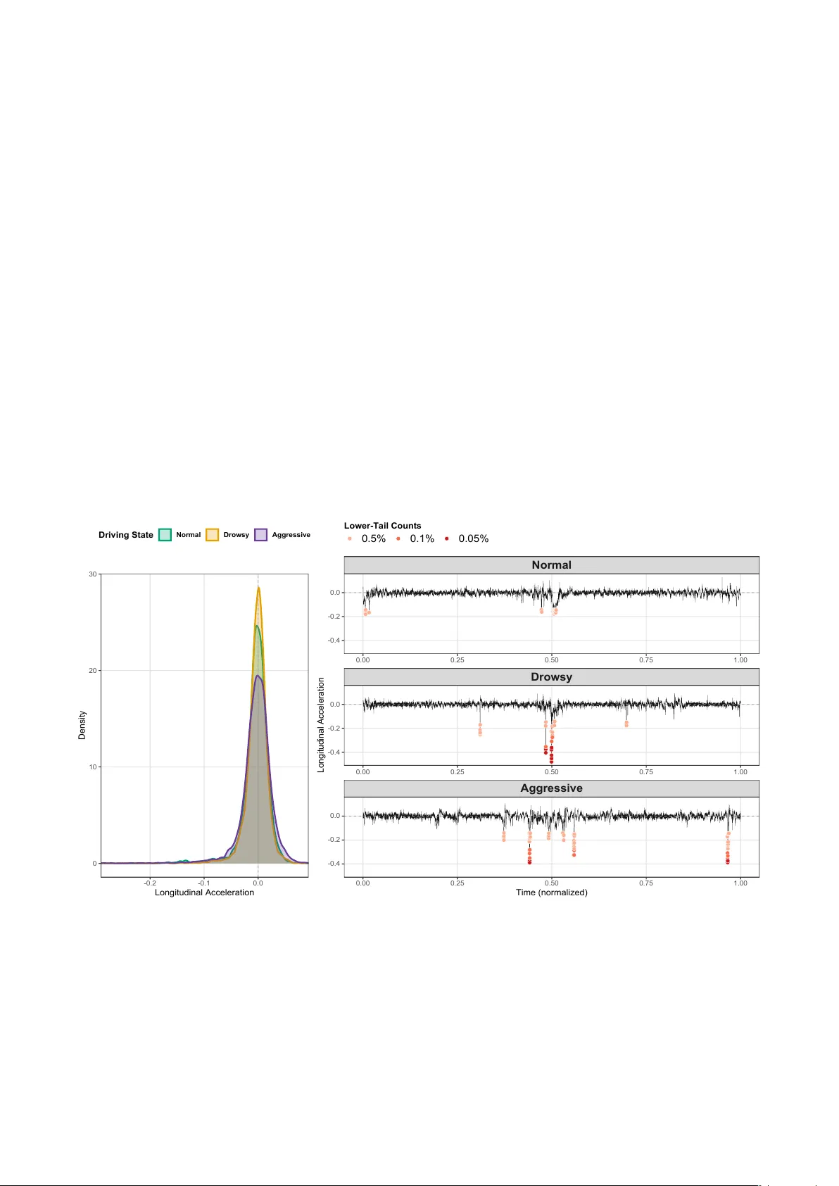
A P or tf olio- Anchored Frequency–Se v er ity Risk Inde x f or T r ip and Dr iv er Assessment Using T elematics Signals Jongtaek Lee, Andrei Badescu, X. Sheldon Lin Depar tment of S tatistical Sciences, U niversity of T oronto Abstract In this paper , w e propose a no v el frequency–sev erity joint trip-lev el risk index that combines the frequency of abnormal dr iving patterns with a sev er ity component reflecting ho w extreme suc h beha vior is relative to a por tf olio-lev el baseline. Sev er ity is quantified through an in verse-probability penalty that increases with the rarity of observ ed tail e xtremes, rather than being inter preted as a claim size. Based on high-frequency telematics data, w e cons truct a multi-scale representation of longitudinal acceleration using the maximal o ver lap discrete wa velet transf or m (MOD WT), which preserves localized driving patter ns across multiple time scales. T o capture se v er ity as tail rarity , we model the portfolio distribution using a Gaussian–U nif or m mixture with a la yered tail s tr ucture, where Gaussian components descr ibe typical driving beha vior and the tail is par titioned into ordered se v er ity la yers that reflect increasing e xtremeness. W e dev elop a likelihood-based estimation procedure that makes inference feasible f or this mixture model. The resulting sev er ity la y ers are then used to construct multi-lay er tail counts (ML TC) at the tr ip lev el, whic h are modeled within a Poisson–Gamma frame work to yield a closed-f orm posterior r isk inde x that jointly reflects frequency and se verity . This conjugate str ucture naturall y suppor ts sequential updating, enabling the construction of dynamically ev olving dr iv er -lev el r isk profiles. Using the U AH-Dr iv eSet controlled dataset, we demons trate that the proposed index enables reliable discrimination across behavioral dr iving states, identification of high-r isk trips, and coherent ranking of dr iv ers, yielding a purely beha vior -dr iv en r isk measure suitable f or actuarial ratemaking and potentially mitigating f air ness concerns associated with traditional co variates. Ke yw ords: T elematics signal, maximal o v erlap wa velet transf or m, multiple time scales, Gaussian-Unif or m mixture model, MU-MEMR, tail la yers, por tf olio distribution, se v er ity w eights, P oisson–Gamma s tr ucture, frequency –sev er ity joint tr ip-le v el r isk inde x. 1 Introduction T raditional auto insurance ratemaking relies pr imarily on static driver and v ehicle characteristics, which are typicall y e valuated at discrete points in time (e.g., annually). While these co variates are inf or mativ e f or assessing long-term or av erage r isk lev els, they are inherently limited in their ability to capture real-time driving behavior , as they are only indirectly related to the instantaneous risk of an accident, see Chan et al. (2025a), V erbelen et al. (2018). For the same reason, because these co variates are inherently attached to the dr iv er or v ehicle, pr icing is typicall y conducted at the dr iv er lev el and remains largel y static ov er time, 1 rather than being dynamically adjusted from trip to tr ip. With recent technological advances enabling high-frequency data collection, telematics has emerg ed as a means to address the limitations of traditional ratemaking. This shift suppor ts pr icing frame w orks based directly on observed driving beha vior , allo wing insurers to adjust premiums dynamically through usage-based insurance (UBI), see V erbelen et al. (2018). In this conte xt, telematics signals are used to refine r isk prediction b y directly measur ing ho w a vehicle is operated at high temporal resolution. These signals can be incor porated into insurance practice through pricing, screening and under writing, or ongoing monitor ing. Their value is par ticular ly pronounced in settings where claims are sparse, as signal-based approaches allow insurers to infer r isk from observed driving behavior rather than relying solely on infrequent loss realizations. T elematics data compr ise both kinematic signals (e.g., speed, longitudinal and lateral acceleration) and conte xtual inf or mation (e.g., road type, w eather , traffic conditions, and time of day). In practice, ho we ver , such data rarely include g round-truth labels of accident r isk at the tr ip or moment lev el. This absence of labeled outcomes motivates telematics research to f ocus on how effectiv ely r isk -relev ant patterns can be represented and quantified directly from high-frequency signals, rather than relying only on traditional co variates, claims data, or explicit tr ip-le v el labels. The actuar ial telematics literature has rapidly ev ol v ed, pro viding a variety of methods to manage this r ich inf ormation for insurance applications. The first strand f ocuses on “representation and f eature construction ” to turn high-frequency driving records into actuarial co variates, including cov ar iate selection and engineered summar ies from telematics signals Wüthrich (2017), low -dimensional representations such as speed–acceleration heatmaps and related f eature e xtraction frame w orks Gao and Wüthr ich (2018), Gao et al. (2019), as well as broader data mining approaches that unco v er common dr iving patterns from telematics records Chan et al. (2025b). The second strand dev elops “actuarial modeling and pr icing frame w orks ” that incor porate telematics inf ormation into insurance models and rating systems, ranging from credibility -sty le multivariate f ormulations and model-based integ ration Denuit et al. (2019), to assessments of the incremental v alue of dynamic telematics updates Henckaerts and Antonio (2022), bonus–malus sty le scoring f or sequential ratemaking Yáñez et al. (2025), as w ell as empir ical studies on how telematics impro ves claims prediction and classification Meng et al. (2022), Duval et al. (2022), Duv al et al. (2024). Man y approaches in this strand essentiall y reduce high-frequency telematics time series to engineered features or summar y statistics, but a larg e por tion of the temporal structure in the signals has remained unexploited. This compression has limitations in detecting r isk -relev ant patterns that are localized in time. This motivated the third s trand “dr iving dynamics and s tate ev olution ” that lev erages the temporal structure of the signals b y using sequential or latent state models to describe ho w risk -relev ant beha vior unf olds o v er time and how deviations from typical beha vior can be identified Meng et al. (2022), Jiang and Shi (2024), Chan et al. (2025a). In par ticular , Chan et al. (2025a) propose a multivariate Continuous- Time Hidden Marko v Model (CTHMM) to model a tr iv ar iate response compr ising speed, longitudinal acceleration, and lateral acceleration. The y construct an anomaly inde x that quantifies the number of abnor mal behavioral episodes observ ed dur ing a tr ip. While this approach is effectiv e in identifying aggressiv e dr iving patter ns, it seems less successful in captur ing drow sy or inattentiv e beha vior . Despite these methodological adv ances, most telematics-based risk assessments remain fundamentall y fr equency-oriented . Existing approaches primar il y emphasize how of ten abnor mal behavior occurs or the magnitude of deviations from a fitted model, with comparativ ely limited attention to how sever e those beha viors are. Within this tra jectory to w ard increasingl y signal-dr iv en r isk ev aluation, incor porating 2 beha vioral severity as an additional dimension represents a natural and necessar y e xtension to achie v e a more refined and comprehensive r isk assessment framew ork. 1.1 Data and Preliminary Analy sis This section descr ibes the data that will be used in this paper and presents a preliminar y analy sis to justify the introduction of telematics sev erity to r isk ev aluation. The analy sis will sho w ho w frequency -based summaries can miss some impor tant r isk -relev ant patter ns and how sev er ity -based summar ies can help a more accurate identification of those patter ns, which motiv ates our fr equency–sev erity joint risk index that will be proposed in the f ollo wing sections. This naturally raises the question of wh y sev er ity information should pro vide a complementar y and practically useful dimension bey ond frequency , which we illustrate ne xt via a simple empirical justification. 1.1.1 Data The U AH-Dr iv eSet introduced by Romera et al. (2016) is a public smar tphone-sensor dataset f or dr iv er beha vior analy sis. In this paper, we use this Controlled Data which was recorded using the DriveSaf e application. The dataset includes recordings from six different dr iv ers with their o wn v ehicles under three beha vioral dr iving states: normal , aggressive , and drowsy . N or mal dr iving reflects typical e veryda y beha vior , aggressive dr iving show s impatience and abr upt maneuv ers such as ov erspeeding or tailgating, and drow sy driving simulates mild sleepiness with occasional inattention. Data w ere collected on tw o pre-specified routes near Alcalá de Henares in the Community of Madr id, Spain: a secondar y road route (about 90 km/h maximum speed) and a motor w a y route (about 120 km/h maximum allo wed speed). Each driver repeats these routes under the three instructed driving states, yielding multiple tr ips per dr iv er on each road type. On the secondary road, each of Dr iv ers 1–5 contr ibutes f our trips (tw o normal repeats, one aggressive , and one drowsy ), whereas on the motorwa y each driver contributes one tr ip per instructed state ( normal , aggressive , drowsy ). The only e x ception is Driver 6, whose electr ic vehicle completes the motorwa y set but provides only normal and drowsy on the secondar y road due to limited v ehicle autonom y . Consequentl y , there are 40 tr ips, and each operated o v er about 8 to 20 minutes. T able 1 summar izes the dr iv ers, vehicles, and the number of tr ips by road type. In this paper , w e solely focus on longitudinal acceleration recorded at 10 Hz (ev er y 0.1 seconds) in units of 𝐺 ( 9 . 8 m / s 2 ), where positive values indicate acceleration and negativ e values indicate braking. This Controlled Data hav e also been analyzed in Chan et al. (2025a), which makes it a useful benchmark f or contrasting different signal-based r isk ev aluation approaches. T able 1: Summar y of the U AH-DRIVESET controlled dataset: dr iv er demographics, v ehicle inf or mation, and the number of av ailable tr ips b y road type (secondar y vs. motor w ay). Driver Gender Ag e V ehicle Fuel Sec. tr ips Mot. trips T otal D1 Male 40–50 Audi Q5 (2014) Diesel 4 3 7 D2 Male 20–30 Mercedes B180 (2013) Diesel 4 3 7 D3 Male 20–30 Citroën C4 (2015) Diesel 4 3 7 D4 Female 30–40 Kia Picanto (2004) Gasoline 4 3 7 D5 Male 30–40 Opel As tra (2007) Gasoline 4 3 7 D6 Male 40–50 Citroën C-Zero (2011) Electric 2 3 5 3 1.1.2 Preliminary Analy sis For a compar ison of the o v erall distributional profiles of different dr iving s tates, the empir ical densities f or longitudinal acceleration of Dr iv er 1’ s three motor w a y tr ips are display ed in Panel (a) in Figure 1. In the panel, w e can see that the nor mal and drow sy tr ips both concentrate near zero, and the dro wsy tr ip places e ven more mass around zero than the nor mal tr ip. This illustrates the difficulty of identifying r isk -relev ant patterns of the dro wsy or inattentive tr ip because it looks ev en safer than nor mal from a distributional perspectiv e. In the f ollo wing, we call this nor mal-looking profile . This nor mal-looking profile implies that r isk -relev ant differences ma y be hidden in the tails rather than in the bulk of the distribution, so there is a need to conduct a closer ex amination of the structural difference among the dr iving states of a driver b y inspection of their tail beha viors. W e apply simple quantile lay ers to e xamine the tail structure. These quantile la yers here are only a descriptive pro xy to illustrate tail depth, while later sections define severity f ormally using our proposed model. W e compute the pooled lo wer tail quantiles based on the three trips and then commonly apply them to all the trips, as shown in Panel (b) in Figure 1. Specifically , we combine all acceleration obser v ations across the tr ips into one sample and compute its 0 . 5% , 0 . 1% , and 0 . 05% lo w er tail quantiles, denoted by 𝑞 0 . 5% , 𝑞 0 . 1% , and 𝑞 0 . 05% . V alues below these thresholds represent increasingly sev ere deceleration-relev ant patterns, and T able 2 repor ts the cor responding lay er counts. 0 10 20 30 -0.2 -0.1 0.0 Longitudinal Acceleration Density Driving State Normal Drowsy Aggressive Aggressive Drowsy 0.00 0.25 0.50 0.75 1.00 0.00 0.25 0.50 0.75 1.00 Normal 0.00 0.25 0.50 0.75 1.00 -0.4 -0.2 0.0 -0.4 -0.2 0.0 -0.4 -0.2 0.0 Time (normalized) Longitudinal Acceleration Lower-Tail Counts 0.5% 0.1% 0.05% Figure 1: Dr iv er 1 motorwa y e xample: longitudinal acceleration densities (left) and tr ip trajectories with pooled left-tail thresholds marked at the 0.5%, 0.1%, and 0.05% quantiles (r ight), illustrating how tail observations are tur ned into ML TC ev ents. The result show s that multiple depths in the tails car ry inf or mation that a frequency -based summar y with a single threshold can miss. For e xample, if one only counts e xceedances be y ond 𝑞 0 . 5% , the nor mal trip w ould appear riskier than the drow sy tr ip (sum of e xceedances are 41 v ersus 21 + 3 + 7 = 31 ). In contrast, the deeper lay ers rev eal that the dro wsy tr ip places more mass in the extreme tail. The drow sy 4 trip has 3 e x ceedances in ( 𝑞 0 . 05% , 𝑞 0 . 1% ] and 7 e x ceedances below 𝑞 0 . 05% , while the normal trip has none in either lay er, which makes it separable once the sev er ity -based summary is taken into account. This mechanism is consistent with the frequency-based approach in Chan et al. (2025a), under which dro wsy trips in the same Controlled Data were not flagged as r isky by their CTHMM model. This preliminary analy sis pro vides concrete e vidence that incorporating the sev er ity str ucture based on multiple tail-la y ers enables a more refined ev aluation of dr iving behavior in telematics signals. This motivates our frequency –sev er ity joint r isk index to more accurately identify r isky tr ips. T able 2: Dr iv er 1 motorwa y e xample: counts of lo w er -tail observations in the pooled distribution, g rouped into three sev erity lay ers defined by empir ical left-tail quantiles (0.5%, 0.1%, and 0.05%). Driving state # { 𝑞 0 . 1% < · ≤ 𝑞 0 . 5% } # { 𝑞 0 . 05% < · ≤ 𝑞 0 . 1% } # { · ≤ 𝑞 0 . 05% } Normal 41 0 0 Dro wsy 21 3 7 Aggressiv e 39 10 6 1.2 Se v erity La yers and a T rip-Lev el Risk Index The pr imary objective of this paper is to constr uct a frequency–sev er ity joint tr ip-le v el r isk inde x from telematics signals and to demonstrate its effectiv eness in identifying dangerous tr ips and high-r isk dr iv ers. W e fur ther show that the proposed index discr iminates between normal and r isky (i.e., aggressive and dro wsy) dr iving within a classification frame work. V er y impor tantl y , the frame work does not rely on traditional cov ariates, claims data, or r isk labels. Instead, it ev aluates r isk directly at the trip level using telematics signals alone, which aligns with practical UBI settings where claims are sparse. T wo core contr ibutions suppor t this objective. First, we introduce a f or mal notion of sev erity into telematics-based r isk ev aluation, e xtending bey ond purely frequency-based approaches. By decomposing tail behavior into severity layer s and assigning lay er -specific w eights based on por tf olio-lev el rar ity , we obtain a more g ranular characterization of abnor mal patter ns. Second, we dev elop a Gaussian–U niform mixtur e sev er ity model with multiple Unif or m components on each tail, together with an implementable fitting algor ithm described in Section 3. In classical insurance terminology , “sev erity” refers to the loss amount conditional on a claim. Here, w e reinter pret severity as the magnitude of abnor mal longitudinal acceleration, quantified relativ e to its statis tical rar ity in the por tf olio-lev el distribution. Observations lying deeper in the tails receive greater w eight in the proposed inde x. Intuitiv ely , suppose that each telematics signal e xhibits a por tf olio-lev el rang e of typical behavior (e.g., ordinar y braking or tur ning intensity), then patterns that f all substantiall y outside this rang e, such as rare harsh braking or turning episodes, should contr ibute more hea vily to r isk assessment. W e f ormalize this idea through sev er ity la yers that assign increasing w eights to progressiv ely rarer behaviors, independent of claim occur rence. The framew ork integ rates three components. • Signal representation via wa v elet transf orm: W e represent each telematics signal using the Maximal Ov erlap Discrete W a v elet T ransf or m (MOD WT) P ercival and W alden (2013) to capture localized patterns across multiple time scales. Coefficients are agg reg ated across scales into a single tr ip-le v el series summar izing multi-scale behavior , yielding a per -e xposure inde x nor malized f or tr ip length. • P ortf olio-lev el se v erity model: W e construct the portfolio distribution of aggregated wa v elet 5 coefficients and fit a Gaussian–U niform mixture Coretto and Hennig (2011), Coretto (2022), where Gaussian components represent typical behavior and U nif or m components define abnor mal tail beha vior . Estimating sev erity at the por tf olio le vel ensures comparability across trips and dr iv ers. • T rip-le vel freq uency model and risk index: Lay er -wise tr ip counts are modeled using a Poisson– Gamma structure. The proposed r isk index is defined as a sev erity-w eighted per -exposure risk rate across lay ers and can be updated sequentially to produce a dynamic driver -lev el profile. The focus on longitudinal acceleration is deliberate, as pr ior telematics studies ha ve established its rele vance f or detecting r isky dr iving beha vior Chan et al. (2025a), Yáñez et al. (2025), Mao et al. (2021), and it provides a clear and interpretable starting point. The framew ork, moreov er , is signal-agnostic: it can be applied to other telematics responses by fitting the cor responding sev er ity and frequency components, and it can be extended to a multivariate setting by combining signal-specific indices into a composite r isk measure. Suc h extensions are left f or future work. The resulting inde x functions as an anomaly index that jointly accounts f or both the frequency and se verity of abnor mal behaviors within a tr ip. In insurance applications, it yields a per -e xposure tr ip score that can be agg reg ated and updated sequentiall y to maintain an ev olving dr iving r isk profile f or pr icing and under writing in UBI. In transpor tation safety and fleet management, trip-lev el scores can pr ioritize re view and intervention by highlighting the most concerning patterns. More broadl y , the frame w ork pro vides a signal-based screening metric applicable ev en when claims or labeled outcomes are limited. The remainder of the paper is org anized as f ollo ws. Section 2 revie ws the MOD W T representation and across-le vel (-scale) aggregation. Section 3 introduces the Gaussian–Unif orm mixture sev er ity model and its estimation procedure. Section 4 dev elops the P oisson–Gamma frequency model and defines the trip- and driver -le vel frequency–sev er ity indices. Section 5 presents the empir ical application and classification results, and Section 6 concludes and discusses future directions. 2 Discre te W a v elet T ransform f or T elematics Signals In this section, we dev elop a tr ip-le v el representation that will ser v e as input to our proposed r isk index. For each tr ip, we decompose the signal into wa v elet coefficients across multiple time scales and then aggregate these coefficients into a single ser ies that summar izes dr iving patter ns o v er both shor t and long durations. The resulting agg reg ated ser ies is used to form an input por tf olio distr ibution, which is a ke y ingredient of the proposed risk inde x in the subsequent sections. As discussed in Section 1, this representation applies to any telematics signal recorded as a time ser ies and can be extended to a multiv ar iate r isk index that integrates multiple telematics signals in future w ork. T o achie v e this, we emplo y a wav elet transf or m Perciv al and W alden (2013), which is par ticularl y w ell suited f or detecting abnor mal patterns in telematics signals across multiple time scales. T elematics signals typicall y exhibit abr upt, shor t-liv ed ev ents (e.g., harsh braking or acceleration), making global or o v erl y smooth representations less effective. For example, Fourier bases ha ve global suppor t ov er the entire obser v ation windo w and B-spline bases impose smoothness. In contrast, wa velets are explicitl y designed to capture localized f eatures in time: wa v elet bases are localized in time and operate through filters of v ar ying duration, from short to long scales, that concentrate around points of c hange. The resulting w av elet coefficients are theref ore associated with specific time inter v als and scales, enabling precise identification of transient behaviors. This localization proper ty makes the wa v elet transf or m a 6 natural and effective representation f or anal yzing telematics signals and e xtracting r isk -relev ant driving patterns. In this paper , w e use the maximal ov erlap discre te wav elet transf or m (MOD WT) rather than a regular discrete wa velet transf or m (D WT) because it is a better choice for telematics signals when our goal is to detect abnor mal dr iving beha vior while retaining all possible f eatures that could later be identified as abnor mal patter ns. Since the regular D W T does do wnsampling, it critically depends on where w e “break into” the ser ies, i.e., what we take as a star ting point or or igin for analy sis. In other w ords, the regular D W T is sensitiv e to shifts so its filter might not line up well with interesting features in a time series Perciv al and W alden (2013). In contrast, as y ou may ha ve already noticed by the ter m “maximal o v erlap”, the MOD W T applies the wa velet and scaling filters at every time point through circular shifts, considering all possible placements of the filters with the signal. This prev ents missing impor tant dr iving beha viors that occur at arbitrar y times within a tr ip because the MOD WT produces coefficients at ev er y time point without downsampling. W e now f or malize this representation by defining the MOD WT filters and the resulting w a velet and scaling coefficients for each tr ip. These coefficients will be agg reg ated to f or m the input por tf olio distribution f or sev er ity and frequency modeling. 2.1 MOD WT Decomposition and Representation 2.1.1 MOD WT Filters A regular D W T is defined b y two filters: a wav elet filter { ℎ ℓ } 𝐿 − 1 ℓ = 0 and a scaling filter { 𝑔 ℓ } 𝐿 − 1 ℓ = 0 , where 𝐿 is the number of ter ms of the filters. T o effectivel y capture a common characteristic of telematics signals, w e adopt the Daubec hies D4 wa velet filter , with 𝐿 = 4 ter ms, given b y: ℎ 0 = 1 − √ 3 4 √ 2 , ℎ 1 = − 3 + √ 3 4 √ 2 , ℎ 2 = 3 + √ 3 4 √ 2 , ℎ 3 = − 1 − √ 3 4 √ 2 . The cor responding scaling filter is obtained b y 𝑔 ℓ = ( − 1 ) ℓ + 1 ℎ 𝐿 − 1 − ℓ , ℓ = 0 , 1 , 2 , 3 , that is, 𝑔 0 = − ℎ 3 , 𝑔 1 = ℎ 2 , 𝑔 2 = − ℎ 1 , 𝑔 3 = ℎ 0 . T elematics signals often e xhibit shor t-t er m mean rev ersion characteristic: the signal typically mov es back to ward the mean zero ov er the next fe w time points after a burst, which makes Gaussian assumptions f or some telematics signals (e.g., longitudinal or lateral accelerations) reasonable, as demonstrated in Chan et al. (2025a). Another widely used filter is the Haar wa velet filter , that is essentially based on the difference between adjacent values ( ℎ 0 = 1 √ 2 , ℎ 1 = − 1 √ 2 ), so this structure can underestimate the strength of localized deviations due to local cancellation by a v eraging adjacent values a wa y . In contrast, the D4 filter distr ibutes w eights ov er multiple time points, which aligns with the mean rev ersion characteristic. This a v oids underestimating impor tant f eatures in the transf or m domain and helps retain the signature of risk -relev ant patter ns in mean-rev er ting signals. Thus, the D4 filter pro vides a clear representation of meaningful changes in telematics signals. A ke y f eature of the w av elet transf or m is its multi-resolution decomposition : it represents a time ser ies 7 using components that capture chang es o ver different time scales. W e inde x these scales by a level 𝑗 , which cor responds to chang es in the or iginal time ser ies on a scale of 2 𝑗 − 1 . A t finer lev els (small 𝑗 ), the transf orm captures shor t-liv ed, localized chang es, while at coarser lev els (larg e 𝑗 ), it captures smoother chang es that persist o ver long er durations. T o account f or the multi-scale vie w , we denote b y { ℎ 𝑗 , ℓ } 𝐿 𝑗 − 1 ℓ = 0 and { 𝑔 𝑗 , ℓ } 𝐿 𝑗 − 1 ℓ = 0 the filters at lev el 𝑗 obtained from the D WT filters { ℎ ℓ } and { 𝑔 ℓ } b y dyadic dilation (i.e., b y inser ting 2 𝑗 − 1 − 1 zeros betw een successiv e ter ms). For the MOD WT , w e use rescaled filters defined as e ℎ 𝑗 , ℓ = ℎ 𝑗 , ℓ √ 2 , e 𝑔 𝑗 , ℓ = 𝑔 𝑗 , ℓ √ 2 , ℓ = 0 , . . . , 𝐿 𝑗 − 1 , (1) where the filter width at lev el 𝑗 is 𝐿 𝑗 = ( 2 𝑗 − 1 ) ( 𝐿 − 1 ) + 1 , (2) i.e., the number of lags of the or iginal signal ref erences when computing each MOD W T coefficient at le vel 𝑗 . The rescaling ensures the variance contr ibutions across lev els are comparable. Without scaling, the contr ibution w ould be inflated simply because the MOD W T produces coefficients at e very time point. 2.1.2 MOD WT Coefficients T o represent a telematics signal across time scales, we apply MOD W T filters and define its wav elet and scaling coefficients decomposed at each le v el 𝑗 . F or trip 𝑖 , let the telematics signal hav e the length- 𝑇 𝑖 time series X 𝑖 : = ( 𝑋 𝑖 , 𝑡 ) 𝑇 𝑖 − 1 𝑡 = 0 . Giv en the MOD W T filters in (1), the cor responding coefficients at lev el 𝑗 are defined b y e 𝑊 𝑖 , 𝑗 , 𝑡 : = 𝐿 𝑗 − 1  ℓ = 0 e ℎ 𝑗 , ℓ 𝑋 𝑖 , ( 𝑡 − ℓ ) mod 𝑇 𝑖 , e 𝑉 𝑖 , 𝑗 , 𝑡 : = 𝐿 𝑗 − 1  ℓ = 0 e 𝑔 𝑗 , ℓ 𝑋 𝑖 , ( 𝑡 − ℓ ) mod 𝑇 𝑖 , 𝑡 = 0 , . . . , 𝑇 𝑖 − 1 , (3) where ( 𝑡 − ℓ ) mod 𝑇 𝑖 denotes circular inde xing that maps any integer to an element of { 0 , 1 , . . . , 𝑇 𝑖 − 1 } . For an y integer 𝐽 ≥ 1 , the vectors ha ve the f ollo wing inter pretations: • a v ector f W 𝑖 , 𝑗 contains the MOD WT wa v elet coefficients associated with chang es in X 𝑖 on a scale of 2 𝑗 − 1 f or 𝑗 = 1 , . . . , 𝐽 , • and a v ector e V 𝑖 , 𝐽 contains the MOD W T scaling coefficients associated with changes in X 𝑖 on a scale 2 𝐽 or higher, where f W 𝑖 , 𝑗 = ( e 𝑊 𝑖 , 𝑗 , 𝑡 ) 𝑇 𝑖 − 1 𝑡 = 0 and e V 𝑖 , 𝐽 = ( e 𝑉 𝑖 , 𝐽 , 𝑡 ) 𝑇 𝑖 − 1 𝑡 = 0 P ercival and W alden (2013) and 𝐽 is the chosen maximum le vel of the MOD WT decomposition. Since the filter width 𝐿 𝑗 increases with 𝑗 , the coefficients at finer lev els represent localized f eatures and coarser le vels represent milder f eatures with longer duration. This multi-resolution structure across lev els can capture both br ief ev ents and sustained patter ns that can be informativ e dr iving behaviors. The wa v elet filters and coefficients in (3) pro vide a complete representation of the or iginal time ser ies X 𝑖 . F or each lev el 𝑗 , w e e xtend the filters { e ℎ 𝑗 , ℓ } 𝐿 𝑗 − 1 ℓ = 0 and { e 𝑔 𝑗 , ℓ } 𝐿 𝑗 − 1 ℓ = 0 to length 𝑇 𝑖 b y setting e ℎ 𝑗 , ℓ = 0 and 8 e 𝑔 𝑗 , ℓ = 0 f or ℓ = 𝐿 𝑗 , . . . , 𝑇 𝑖 − 1 . Then, we represent X 𝑖 using 𝑋 𝑖 , 𝑡 = 𝐽  𝑗 = 1 𝑇 𝑖 − 1  ℓ = 0 e ℎ 𝑗 , ℓ e 𝑊 𝑖 , 𝑗 , ( 𝑡 + ℓ ) mod 𝑇 𝑖 + 𝑇 𝑖 − 1  ℓ = 0 e 𝑔 𝐽 , ℓ e 𝑉 𝑖 , 𝐽 , ( 𝑡 + ℓ ) mod 𝑇 𝑖 , (4) f or a given 𝐽 ≥ 1 . Under the circular inde xing con v ention in (3) , this reconstruction holds f or all 𝑡 = 0 , . . . , 𝑇 𝑖 − 1 , so X 𝑖 can be recov ered from { f W 𝑖 , 𝑗 } 𝐽 𝑗 = 1 and e V 𝑖 , 𝐽 . This wa v elet transf orm is par ticularl y useful in UBI settings where w e need to focus on signal-based analy sis rather than sparse claim counts because this representation allo ws us to map each tr ip to a coefficient ser ies that retains the full signal inf ormation, which will serve as the f oundation f or our r isk indices. 2.2 Energy Decomposition and Aggregation 2.2.1 Energy and V ariance Contributions As the lev el 𝑗 increases, coefficients bey ond a cer tain lev el tend to represent onl y broad baseline mo vement, which is around zero, rather than meaningful risk -relev ant maneuv ers in a telematics signal. F or this reason, choosing the maximum lev el of the decomposition 𝐽 is a natural question to select a meaningful set of lev els, and w e theref ore quantify the contribution of each lev el 𝑗 to tr ip 𝑖 using the MOD W T energy decomposition. F or a fixed integer 𝐽 ≥ 1 , Perciv al and W alden (2013) pro v ed that the MOD W T yields the energy decomposition ∥ X 𝑖 ∥ 2 = 𝐽  𝑗 = 1 ∥ f W 𝑖 , 𝑗 ∥ 2 + ∥ e V 𝑖 , 𝐽 ∥ 2 , (5) because we hav e ∥ f W 𝑖 , 𝑗 ∥ 2 + ∥ e V 𝑖 , 𝑗 ∥ 2 = ∥ e V 𝑖 , 𝑗 − 1 ∥ 2 , 𝑗 = 1 , 2 , . . . with the definition e V 𝑖 , 0 : = X 𝑖 and ∥ · ∥ denotes the ℓ 2 norm. T o quantify contr ibutions f or each lev el, we define a sample variance of X 𝑖 b y b 𝜎 2 X 𝑖 : = 1 𝑇 𝑖 ∥ X 𝑖 ∥ 2 − 𝑋 2 𝑖 , where 𝑋 𝑖 : = 𝑇 − 1 𝑖 Í 𝑇 𝑖 − 1 𝑡 = 0 𝑋 𝑖 𝑡 . F or each lev el 𝑗 , define the energy component V 𝑖 ( 𝑗 ) : = 1 𝑇 𝑖   f W 𝑖 , 𝑗   2 , yielding the variance contribution given b y 𝜌 𝑖 , 𝑗 : = V 𝑖 ( 𝑗 ) b 𝜎 2 X 𝑖 , 𝑗 = 1 , . . . , 𝐽 . (6) where 𝜌 𝑖 , 𝑗 ∈ [ 0 , 1 ] and the cumulativ e sum typically increases as 𝐽 increases. This v ar iance contr ibution 𝜌 𝑖 , 𝑗 will be used f or a practical choice of the decomposition depth 𝐽 in Section 5. In par ticular , since the incremental contr ibution 𝜌 𝑖 , 𝑗 typicall y decreases as 𝑗 increases, we can identify a cutoff lev el bey ond which additional scales contr ibute negligibl y to the o verall v ar iance and are theref ore treated as practicall y insignificant for the representation. 9 2.2.2 A cross-le vel Aggregation Risk -relev ant patter ns in telematics signals do not occur in a single time scale within a tr ip, so a tr ip-le v el representation should capture both shor t- and long-duration f eatures. W e theref ore aggregate MOD W T w av elet coefficients f W 𝑖 , 𝑗 across lev els into a single time series which summar izes multi-scale patter ns. In addition, this across-lev el aggregation enables a per -exposure r isk inde x nor malized for the tr ip length via an exposure offset, as will be descr ibed in Section 4. For a set of lev els J ⊂ { 1 , . . . , 𝐽 } , we define the aggr eg ated wav elet coefficient f or a trip 𝑖 at each time point 𝑡 as 𝐶 𝑖 , 𝑡 : = 𝔤  { e 𝑊 𝑖 , 𝑗 , 𝑡 } 𝑗 ∈ J  , 𝑡 = 0 , . . . , 𝑇 𝑖 − 1 , (7) where { e 𝑊 𝑖 , 𝑗 , 𝑡 } 𝑗 ∈ J is the collection of the MOD WT coefficients across lev els at time point 𝑡 and 𝔤 : R | J | → R is the aggregation function. There are some practical choices of 𝔤 ( · ) based on how the coefficients are agg reg ated across lev els: • a maximum choice 𝐶 𝑖 , 𝑡 = max 𝑗 ∈ J | e 𝑊 𝑖 , 𝑗 , 𝑡 | , • an av erage pooling 𝐶 𝑖 , 𝑡 = | J | − 1 Í 𝑗 ∈ J | e 𝑊 𝑖 , 𝑗 , 𝑡 | , • a weighted pooling 𝐶 𝑖 , 𝑡 = Í 𝑗 ∈ J 𝜔 𝑗 | e 𝑊 𝑖 , 𝑗 , 𝑡 | with weights 𝜔 𝑗 ≥ 0 and Í 𝑗 ∈ J 𝜔 𝑗 = 1 , • a single-lev el choice 𝐶 𝑖 , 𝑡 = e 𝑊 𝑖 , 𝑗 ∗ , 𝑡 f or a fixed 𝑗 ∗ ∈ J . The choice of the aggregation r ule depends on the nature of data and the goal of the analy sis. This agg reg ation produces a single time ser ies of the aggregated wa v elet coefficients f or tr ip 𝑖 C 𝑖 = ( 𝐶 𝑖 , 0 , . . . , 𝐶 𝑖 , 𝑇 𝑖 − 1 ) , (8) which summar izes { e 𝑊 𝑖 , 𝑗 , 𝑡 } 𝑗 ∈ J across 𝐽 le vels at each time point. Reg ardless of the choice of 𝔤 ( · ) , C 𝑖 is designed to aggregate dr iving beha viors that may appear at different temporal scales into a time ser ies. In Section 3 and Section 4, C 𝑖 will be an ing redient to build a por tf olio distr ibution that is the input f or our proposed framew ork. 3 Se v erity Model T o define sev er ity at the por tf olio lev el f or tr ip-le v el r isk ev aluation, w e need a stable baseline that is not o v erl y sensitiv e to individual tr ips or dominant dr iving sty les in the por tf olio. In this section, w e theref ore model the por tf olio distribution using a sev er ity model that absorbs tail behavior while preser ving a stable representation of typical dr iving. The estimated sev er ity str ucture will be used in Section 4 to build the joint frequency–se v er ity r isk index. 3.1 Motiv ation and General Description of the Model Longitudinal acceleration is often modeled as Gaussian, Chan et al. (2025a), due to its shor t-term mean re version as discussed in Section 2; ho we ver , a pure Gaussian fit can be distorted by tail v alues that inflate the fitted variance. Moreov er , residual-based outlier measures relativ e to a fitted model proposed b y Chan et al. (2025a) can be sensitive to ho w the “nor mal” reference is defined, because they implicitly assume 10 the fitted model as nor mal driving, which may be biased when the training por tf olio is dominated b y a par ticular dr iving sty le. In this paper , we adopt a Gaussian–U niform mixtur e model Coretto and Hennig (2011) to separate the normal baseline from abnor mal tail behavior . The Gaussian component is dedicated to representing typical dr iving, whereas Unif or m components absorb tail obser v ations. Consequentl y , the Gaussian component remains stable agains t variance inflation, and the baseline used f or sev erity modeling becomes less dependent on por tf olio composition or some par ticular driving sty les. This yields a more robust ref erence distribution f or the sev er ity str ucture. U nif or m endpoints make the mixture likelihood discontinuous, so Coretto (2022) proposed Multiple Expectation–Maximization Runs (MEMR) to make fitting feasible for a model with a single Unif or m component. Ne v er theless, EM fitting still remains difficult and unsolv ed under multiple Unif or m components. In this paper , w e e xtend the MEMR to multiple U nif or m components and propose a Multi-U niform MEMR (MU-MEMR) algorithm, where each Unif or m component defines its own se verity la y er . U nif or m components assigned to deeper tail inter v als represent higher sev er ity , while those closer to the Gaussian core represent lo wer se verity . This nov el e xtension is central to our sev erity framew ork because it enables a direct quantification of sev er ity in ter ms of rar ity in dr iving patter ns. W e define a por tf olio distribution of agg reg ated wa velet coefficients (8) as the input to the Gaussian– U nif or m sev erity model. The mixture model provides robustness conditional on the chosen por tf olio sample b y isolating typical behavior from tail beha vior; ho w ev er, the estimated baseline can still be affected b y ho w the coefficients are pooled across tr ips. One consideration here is that tr ips ma y include beha vior -ir rele v ant noise, so naiv e pooling can contaminate the baseline. For e xample, rough road sur faces can cause suspicious deviations not driven by the dr iv er’ s maneuv er , and long stop per iods generate man y near -zero coefficients for a tr ip. The other consideration is that agg reg ated coefficients within a tr ip f orm a time ser ies, so naivel y pooling all coefficients can also violate the i.i.d. sampling assumption underl ying likelihood fitting. W e theref ore construct the por tf olio distribution using a balanced sampling scheme that controls both the repr esentativ eness across tr ips and tempor al dependence structure within tr ips. Specificall y , we propose a hierar c hical sampling with within-trip thinning scheme that addresses both considerations. The hierarchical stage balances contr ibutions by drawing (i) a dr iv er unif or ml y and (ii) a tr ip from that dr iv er unif ormly . The thinning stag e then reduces temporal dependence b y retaining coefficients within each selected (or av ailable) trip at time points spaced far enough apar t so that the empirical autocor relation falls belo w a chosen threshold. Pooling these retained coefficients across tr ips yields the por tf olio sample C , which we treat as an appro ximately i.i.d. input when defining and fitting the Gaussian–U nif or m sev er ity model in the f ollowing sections. 3.2 Lik elihood and Parame ter Estimation R ecall the agg reg ated wa velet coefficient ser ies C 𝑖 = { 𝐶 𝑖 𝑡 } 𝑇 𝑖 − 1 𝑡 = 0 f or each tr ip 𝑖 , defined in Section 2. T o fit the sev erity model, we construct a por tf olio sample C using the sampling scheme discussed abov e. Let T 𝑖 ⊂ { 0 , . . . , 𝑇 𝑖 − 1 } denote the set of re tained time points after thinning f or a selected tr ip 𝑖 . W e then f orm the por tf olio sample b y pooling the retained coefficients, C : = { 𝐶 𝑟 } 𝑛 𝑟 = 1 = Ø 𝑖 { 𝐶 𝑖 𝑡 : 𝑡 ∈ T 𝑖 } , 𝑛 =  𝑖 | T 𝑖 | , 11 where 𝑟 is a re-inde xing of the retained ( 𝑖 , 𝑡 ) pairs. Then, we model the por tf olio sample C as an appro ximately i.i.d. sample from a Gaussian–Unif or m mixture model. For 𝑔 = 1 , . . . , 𝐺 , define a famil y of Gaussian densities 𝜙  𝑐 𝑟 ; 𝜃 𝑔  with full suppor t on R , where 𝜃 𝑔 = ( 𝜇 𝑔 , 𝜎 𝑔 ) ∈ R × ( 0 , +∞) represents the mean and standard deviation, respectiv ely . Let 𝑚 = 1 , . . . , 𝑀 + inde x a collection of U niform densities 𝑢  𝑐 𝑟 ; 𝜃 + 𝑚  on the right tail of the mixture model, where 𝜃 + 𝑚 = ( 𝑢 + 𝑚 , 𝑢 + 𝑚 + 1 ) ∈ R 2 denotes the unif or m suppor t. Let 𝑚 ′ = 1 , . . . , 𝑀 − inde x U nif or m densities 𝑢  𝑐 𝑟 ; 𝜃 − 𝑚 ′  on the left tail, with the suppor t 𝜃 − 𝑚 ′ = ( 𝑢 − 𝑚 ′ + 1 , 𝑢 − 𝑚 ′ ) ∈ R 2 . Denote the membership probabilities b y 𝜋 𝑔 f or each Gaussian, 𝜋 + 𝑚 f or each r ight-tail Unif orm, and 𝜋 − 𝑚 ′ f or each left-tail U nif or m component. These satisfy 𝜋 − 𝑚 ′ , 𝜋 𝑔 , 𝜋 + 𝑚 ∈ ( 0 , 1 ) and 𝑀 −  𝑚 ′ = 1 𝜋 − 𝑚 ′ + 𝐺  𝑔 = 1 𝜋 𝑔 + 𝑀 +  𝑚 = 1 𝜋 + 𝑚 = 1 . Let 𝑍 𝑟 be a latent variable that labels which component generates 𝐶 𝑟 . The suppor t of 𝑍 𝑟 consists of 𝑀 − left-tail U nif or m components, 𝐺 Gaussian components, and 𝑀 + right-tail U nif or m components. The prior probabilities are Pr ( 𝑍 𝑟 = 𝑚 ′ ) = 𝜋 − 𝑚 ′ , Pr ( 𝑍 𝑟 = 𝑔 ) = 𝜋 𝑔 , Pr ( 𝑍 𝑟 = 𝑚 ) = 𝜋 + 𝑚 , and conditionally on 𝑍 𝑟 w e hav e 𝐶 𝑟 | 𝑍 𝑟 = 𝑚 ′ ∼ 𝑢  • ; 𝜃 − 𝑚 ′  , 𝐶 𝑟 | 𝑍 𝑟 = 𝑔 ∼ 𝜙  • ; 𝜃 𝑔  , 𝐶 𝑟 | 𝑍 𝑟 = 𝑚 ∼ 𝑢  • ; 𝜃 + 𝑚  . The resulting finite mixture density is 𝑓 ( • ; 𝜂 ) : = 𝑀 −  𝑚 ′ = 1 𝜋 − 𝑚 ′ 𝑢  • ; 𝜃 − 𝑚 ′  + 𝐺  𝑔 = 1 𝜋 𝑔 𝜙  • ; 𝜃 𝑔  + 𝑀 +  𝑚 = 1 𝜋 + 𝑚 𝑢  • ; 𝜃 + 𝑚  . (9) where 𝜂 = ( π , 𝚯 ) is the model parameter v ector with π =  { 𝜋 − 𝑚 ′ } 𝑀 − 𝑚 ′ = 1 , { 𝜋 𝑔 } 𝐺 𝑔 = 1 , { 𝜋 + 𝑚 } 𝑀 + 𝑚 = 1  and 𝚯 =  { 𝜃 − 𝑚 ′ } 𝑀 − 𝑚 ′ = 1 , { 𝜃 𝑔 } 𝐺 𝑔 = 1 , { 𝜃 + 𝑚 } 𝑀 + 𝑚 = 1  . Giv en a realization c = { 𝑐 1 , 𝑐 2 , . . . , 𝑐 𝑛 } of the por tf olio sample C , the log-likelihood function is 𝑙 𝑛 ( 𝜂 ) = 𝑛  𝑟 = 1 log 𝑓  𝑐 𝑟 ; 𝜂  . At iteration ℎ = 0 , 1 , 2 , . . . , the poster ior probabilities f or each data point 𝑐 𝑟 and each component are 𝜏 𝑚 ′ ( 𝑐 𝑟 ; 𝜂 ( ℎ ) ) : = Pr ( 𝑍 𝑟 = 𝑚 ′ | 𝐶 𝑟 = 𝑐 𝑟 , 𝜂 ( ℎ ) ) = 𝜋 − ( ℎ ) 𝑚 ′ 𝑢  𝑐 𝑟 ; 𝜃 − ( ℎ ) 𝑚 ′  𝑓  𝑐 𝑟 ; 𝜂 ( ℎ )  , 𝑚 ′ = 1 , . . . , 𝑀 − , 𝜏 𝑔 ( 𝑐 𝑟 ; 𝜂 ( ℎ ) ) : = Pr ( 𝑍 𝑟 = 𝑔 | 𝐶 𝑟 = 𝑐 𝑟 , 𝜂 ( ℎ ) ) = 𝜋 ( ℎ ) 𝑔 𝜙  𝑐 𝑟 ; 𝜃 ( ℎ ) 𝑔  𝑓  𝑐 𝑟 ; 𝜂 ( ℎ )  , 𝑔 = 1 , . . . , 𝐺 , 𝜏 𝑚 ( 𝑐 𝑟 ; 𝜂 ( ℎ ) ) : = Pr ( 𝑍 𝑟 = 𝑚 | 𝐶 𝑟 = 𝑐 𝑟 , 𝜂 ( ℎ ) ) = 𝜋 + ( ℎ ) 𝑚 𝑢  𝑐 𝑟 ; 𝜃 + ( ℎ ) 𝑚  𝑓  𝑐 𝑟 ; 𝜂 ( ℎ )  , 𝑚 = 1 , . . . , 𝑀 + . 12 The EM formulation leads to 𝑄 ( 𝜂 ; 𝜂 ( ℎ ) ) = 𝑛  𝑟 = 1 𝑀 −  𝑚 ′ = 1 𝜏 𝑚 ′ ( 𝑐 𝑟 ; 𝜂 ( ℎ ) ) log 𝑢 ( 𝑐 𝑟 ; 𝜃 − 𝑚 ′ ) + 𝑛  𝑟 = 1 𝐺  𝑔 = 1 𝜏 𝑔 ( 𝑐 𝑟 ; 𝜂 ( ℎ ) ) log 𝜙 ( 𝑐 𝑟 ; 𝜃 𝑔 ) + 𝑛  𝑟 = 1 𝑀 +  𝑚 = 1 𝜏 𝑚 ( 𝑐 𝑟 ; 𝜂 ( ℎ ) ) log 𝑢 ( 𝑐 𝑟 ; 𝜃 + 𝑚 ) + 𝑛  𝑟 = 1 " 𝑀 −  𝑚 ′ = 1 𝜏 𝑚 ′ ( 𝑐 𝑟 ; 𝜂 ( ℎ ) ) log 𝜋 − 𝑚 ′ + 𝐺  𝑔 = 1 𝜏 𝑔 ( 𝑐 𝑟 ; 𝜂 ( ℎ ) ) log 𝜋 𝑔 + 𝑀 +  𝑚 = 1 𝜏 𝑚 ( 𝑐 𝑟 ; 𝜂 ( ℎ ) ) log 𝜋 + 𝑚 # , which decomposes accordingly : 𝑄  𝜂 ; 𝜂 ( ℎ )  = 𝑄 𝑢 −  𝜃 𝑢 − , 𝜂 ( ℎ )  + 𝑄 𝜙  𝜃 𝜙 , 𝜂 ( ℎ )  + 𝑄 𝑢 +  𝜃 𝑢 + , 𝜂 ( ℎ )  + 𝑄 𝜋  𝜃 𝜋 , 𝜂 ( ℎ )  . 3.3 Multi-U niform MEMR Algorithm W e no w descr ibe the fitting algor ithm f or the proposed MU-MEMR estimation procedure. The ke y difference from MEMR is the structure of tail lay ers. W e split each tail into equall y spaced par titions with resolutions 𝑞 and 𝑝 , and, at each iteration, we select 𝑀 − and 𝑀 + tail la y ers from these par titions. W e then r einitialize the U nif or m parameters using the selected lay ers and r un EM f or the Gaussian components and membership probabilities. This candidate searc h makes EM fitting feasible f or a Gaussian–Unif or m mixture with multiple Unif or m components. For a robust initialization for the Gaussian components, we start with trimmed-k-means Cuesta- Alber tos et al. (1997). The parameters are not affected by e xtreme values because it clusters the central bulks after trimming the most extreme 𝛼 % observations in C . This also naturall y provides the base grid f or the candidate search f or U nif or m parameters, given b y the tr immed obser v ations assigned to each tail. Let c − =  𝑐 − 1 , 𝑐 − 2 , . . .  , c + =  𝑐 + 1 , 𝑐 + 2 , . . .  , denote the tr immed observations assigned to the left and r ight tails, respectivel y . Define 𝑐 − min = min ( c − ) , 𝑐 − max = max ( c − ) , 𝑐 + min = min ( c + ) , 𝑐 + max = max ( c + ) , with 𝑐 − max < 0 < 𝑐 + min b y construction of the left and r ight tails. W e split [ 𝑐 − min , 𝑐 − max ] and [ 𝑐 + min , 𝑐 + max ] into 𝑞 and 𝑝 equall y spaced par titions, respectivel y , and set each split point to the nearest obser v ed value in c − and c + when no obser vation lies exactl y on it. This yields ordered points, 𝑏 − ( · ) , 𝑏 + ( · ) : 𝑐 − min < 𝑏 − ( 1 ) < 𝑏 − ( 2 ) < · · · < 𝑏 − ( 𝑞 ) ≤ 𝑐 − max < 0 , 0 < 𝑐 + min ≤ 𝑏 + ( 1 ) < 𝑏 + ( 2 ) < · · · < 𝑏 + ( 𝑝 ) < 𝑐 + max . W e define the base g rid f or U nif or m components as U − =  𝑏 − ( 1 ) , . . . , 𝑏 − ( 𝑞 )  , U + =  𝑏 + ( 1 ) , . . . , 𝑏 + ( 𝑝 )  , 13 where U = U − ∪ U + . F or giv en ( 𝑀 − , 𝑀 + ) , each MU-MEMR r un restr icts the U nif or m endpoints  𝑢 − 𝑀 − + 1 , . . . , 𝑢 − 1 , 𝑢 + 1 , . . . , 𝑢 + 𝑀 + + 1  to build a candidate set. Then, w e repeat the initialization for Unif or m components within the set by selecting  𝑞 𝑀 −  left-tail internal endpoints from the left base gr id U − and  𝑝 𝑀 +  right-tail inter nal endpoints from the right base gr id U + . Increasing 𝑞 and 𝑝 refines the resolution of tail-la yers and yields a sie v e-MLE vie w Grenander (1981), Geman and Hwang (1982) because the base gr id then yields an increasingly fine appro ximation to the continuous parameter space of all possible endpoints. T o obtain stable estimation and an inter pretable sev er ity str ucture, we restrict the Gaussian–U nif or m mixture parameters to a space defined by f our constraints. One constraint controls component scales to a v oid degenerate fits, and the other three define the sev er ity structure by separating tails from the Gaussian core, cov er ing the full tail range with consecutive U nif or m lay ers, and enf orcing monotone membership probabilities for U nif or m components. Firs t, w e impose a scale constr aint to both Gaussian and U niform components. Day (1969) demonstrated the unboundedness of the likelihood function of a Gaussian mixture when some scale parameter 𝜎 𝑔 → 0 f or a fixed mean 𝜇 𝑔 . An analogous phenomenon occurs f or Unif or m components if 𝑢 𝑚 + 1 → 𝑢 𝑚 , f or a fix ed 𝑢 𝑚 T anaka and T akemura (2006). T o ensure the consistency of the MLE, we restrict a lo wer bound exp ( − 𝑛 𝑑 ) ≤ 𝑣 𝑗 f or all 𝑗 , where 𝑣 𝑗 =                    𝑢 − 𝑚 ′ − 𝑢 − 𝑚 ′ + 1 √ 12 if 𝑗 index es 𝑚 ′ = 1 , . . . , 𝑀 − , 𝜎 𝑔 if 𝑗 index es 𝑔 = 1 , . . . , 𝐺 , 𝑢 + 𝑚 + 1 − 𝑢 + 𝑚 √ 12 if 𝑗 index es 𝑚 = 1 , . . . , 𝑀 + , with 𝑛 the sample size of c and 𝑑 ∈ ( 0 , 1 ) T anaka and T akemura (2006). Second, we impose a tail-separation constr aint Coretto (2022) to keep the Unif or m tails separated from the Gaussian cores. W e require 𝑢 − 1 ≤ 𝜇 1 − 𝛿 𝜎 1 , 𝜇 𝐺 + 𝛿 𝜎 𝐺 ≤ 𝑢 + 1 , where 𝜇 1 ≤ · · · ≤ 𝜇 𝐺 and 𝛿 > 0 is fix ed. Here 𝛿 controls the o v erlap between the Gaussian cores and the U nif or m tails. Third, we impose a tail cov erag e constraint . W e fix the extreme tail endpoints as 𝑢 − 𝑀 − + 1 = 𝑐 − min and 𝑢 + 𝑀 + + 1 = 𝑐 + max , treating them as fixed outer parameters of the outer most U nif or m components. W e then set the Unif or m suppor ts to be consecutiv e inter v als that share boundar ies: 𝜃 − 𝑚 ′ = ( 𝑢 − 𝑚 ′ + 1 , 𝑢 − 𝑚 ′ ) , 𝑚 ′ = 1 , . . . , 𝑀 − , 𝜃 + 𝑚 = ( 𝑢 + 𝑚 , 𝑢 + 𝑚 + 1 ) , 𝑚 = 1 , . . . , 𝑀 + . This constraint co v ers the full tail range and assigns e v er y tail obser v ation to e xactly one Unif or m component. Fourth, w e impose a monotonicity constraint on Unif or m membership probabilities f or each tail so that deeper la y ers represent higher sev er ity . With tail lay ers ordered from least extreme to most extreme, 14 w e require 𝜋 − 1 ≥ 𝜋 − 2 ≥ · · · ≥ 𝜋 − 𝑀 − , 𝜋 + 1 ≥ 𝜋 + 2 ≥ · · · ≥ 𝜋 + 𝑀 + . W e enforce these inequalities using isotonic reg ression R ober tson et al. (1988). In each M-step, isotonic regression projects the updated probabilities onto the set of non-increasing sequences, while the ones f or Gaussian components remain unchanged. Then, w e seek the maximizer of the log-likelihood 𝑙 𝑛 ( 𝜂 ) o v er the f ollowing constrained parameter space: 𝜂 𝑛 : =                        𝜂 ∈ η               𝑣 𝑗 ≥ e xp ( − 𝑛 𝑑 ) f or all 𝑗 , 𝑢 − 1 ≤ 𝜇 1 − 𝛿 𝜎 1 , 𝜇 𝐺 + 𝛿 𝜎 𝐺 ≤ 𝑢 + 1 , 𝑐 − min = 𝑢 − 𝑀 − + 1 , 𝑐 + max = 𝑢 + 𝑀 + + 1 , 𝜃 − 𝑚 ′ = ( 𝑢 − 𝑚 ′ + 1 , 𝑢 − 𝑚 ′ ) , 𝜃 + 𝑚 = ( 𝑢 + 𝑚 , 𝑢 + 𝑚 + 1 ) f or all 𝑚 ′ , 𝑚 , 𝜋 − 1 ≥ 𝜋 − 2 ≥ · · · ≥ 𝜋 − 𝑀 − , 𝜋 + 1 ≥ 𝜋 + 2 ≥ · · · ≥ 𝜋 + 𝑀 +                        , with 𝑑 ∈ ( 0 , 1 ) . The constrained maximum-likelihood estimator is then ˆ 𝜂 𝑛 = arg max 𝜂 ∈ 𝜂 𝑛 𝑙 𝑛 ( 𝜂 ) . W e now introduce the MU-MEMR algorithm that implements this constrained optimization of the Gaussian–U nif or m mixture framew ork. 15 Multi-U niform MEMR (MU-MEMR) Algorithm Input : c , 𝑑 ∈ ( 0 , 1 ) , 𝛼 ∈ ( 0 , 1 ) Initialize 𝜃 𝑔 , 𝜃 𝜋 : Giv en a fix ed 𝐺 , r un trimmed- 𝑘 -means on the dataset c . 𝜇 ( ℎ = 0 ) 𝑔 ← 𝑜 𝑔 , 𝜎 ( ℎ = 0 ) 𝑔 ← max { 𝑣 𝑔 , exp ( − 𝑛 𝑑 ) } , 𝑔 = 1 , . . . , 𝐺 , where ( 𝑜 𝑔 , 𝑣 𝑔 ) are the means and standard deviations of the 𝐺 clusters. F or fixed 𝑀 − , 𝑀 + , 𝜋 − ( ℎ = 0 ) 𝑚 ′ , 𝜋 + ( ℎ = 0 ) 𝑚 ← 𝛼 𝑀 − + 𝑀 + , 𝑚 ′ = 1 , . . . , 𝑀 − , 𝑚 = 1 , . . . , 𝑀 + , 𝜋 ( ℎ = 0 ) 𝑔 ← 1 − 𝛼 𝐺 , 𝑔 = 1 , . . . , 𝐺 . f or each c hoice of index sets 1 ≤ Δ − 1 < · · · < Δ − 𝑀 − ≤ 𝑞 and 1 ≤ Δ + 1 < · · · < Δ + 𝑀 + ≤ 𝑝 suc h that 𝑏 − ( Δ − 𝑚 ′ + 1 ) − 𝑏 − ( Δ − 𝑚 ′ ) ≥ √ 12 e xp ( − 𝑛 𝑑 ) and 𝑏 + ( Δ + 𝑚 + 1 ) − 𝑏 + ( Δ + 𝑚 ) ≥ √ 12 e xp ( − 𝑛 𝑑 ) f or all 𝑚 , 𝑚 ′ do Initialize 𝑠 -th 𝜃 − 𝑚 ′ , 𝜃 + 𝑚 : 𝑢 − ( ℎ = 0 ) 𝑀 − + 1 − 𝑚 ′ ← 𝑏 − ( Δ − 𝑚 ′ ) , 𝑢 + ( ℎ = 0 ) 𝑚 ← 𝑏 + ( Δ + 𝑚 ) , 𝑚 ′ = 1 , . . . , 𝑀 − , 𝑚 = 1 , . . . , 𝑀 + , where 𝑟 index es the combination of ( Δ − 1 , . . . , Δ − 𝑀 − ) and ( Δ + 1 , . . . , Δ + 𝑀 + ) , and 𝑢 − 𝑀 − + 1 ← 𝑐 − min , 𝑢 + 𝑀 + + 1 ← 𝑐 + min are fixed. Set 𝜂 ( ℎ = 0 ) ←  𝜃 − ( ℎ = 0 ) 𝑚 ′ , 𝜃 ( ℎ = 0 ) 𝑔 , 𝜃 + ( ℎ = 0 ) 𝑚 , 𝜃 ( ℎ = 0 ) 𝜋  . P erform the 𝑠 -th EM run: while   𝑙 𝑛  𝜂 ( ℎ + 1 )  − 𝑙 𝑛  𝜂 ( ℎ )    > 𝜀 do E-step: U pdate 𝜏 𝑚 ′ ( 𝑐 𝑟 ; 𝜂 ( ℎ ) ) , 𝜏 𝑔 ( 𝑐 𝑟 ; 𝜂 ( ℎ ) ) , 𝜏 𝑚 ( 𝑐 𝑟 ; 𝜂 ( ℎ ) ) f or all 𝑟 = 1 , . . . , 𝑛 . M1-step ( 𝜇 𝑔 , 𝜎 𝑔 ) : Maximize 𝑄 𝜙  𝜃 𝜙 , 𝜂 ( ℎ )  = 𝑛  𝑟 = 1 𝐺  𝑔 = 1 𝜏 𝑔  𝑐 𝑟 ; 𝜂 ( ℎ )  log 𝜙  𝑐 𝑟 ; 𝜇 𝑔 , 𝜎 𝑔  subject to 𝜎 𝑔 ≥ e xp  − 𝑛 𝑑  f or 𝑔 = 1 , . . . , 𝐺 . M2-step ( 𝜋 𝑚 ′ , 𝜋 𝑔 , 𝜋 𝑚 ): Maximize 𝑄 𝜋  𝜃 𝜋 , 𝜂 ( ℎ )  = 𝑛  𝑟 = 1 " 𝑀 −  𝑚 ′ = 1 𝜏 𝑚 ′ ( 𝑐 𝑟 ; 𝜂 ( ℎ ) ) log 𝜋 − 𝑚 ′ + 𝐺  𝑔 = 1 𝜏 𝑔 ( 𝑐 𝑟 ; 𝜂 ( ℎ ) ) log 𝜋 𝑔 + 𝑀 +  𝑚 = 1 𝜏 𝑚 ( 𝑐 𝑟 ; 𝜂 ( ℎ ) ) log 𝜋 + 𝑚 # subject to 𝜋 − 1 ≥ 𝜋 − 2 ≥ · · · ≥ 𝜋 − 𝑀 − and 𝜋 + 1 ≥ 𝜋 + 2 ≥ · · · ≥ 𝜋 + 𝑀 + . Set 𝜂 ( 𝑠 ) ← 𝜂 ( ℎ + 1 ) . Output: 𝜂 ( 𝑠 ∗ ) such that 𝑠 ∗ = arg max 𝑠 𝑙 𝑛  𝜂 ( 𝑠 )  16 4 Freq uency Model This section proposes tr ip- and driver -lev el r isk indices by combining por tf olio-lev el sev er ity lay ers from Section 3 with trip-lev el la y er frequencies to be modeled in this section. Because the sev er ity is estimated at the por tf olio lev el, all trips share the same la yers and cor responding sev er ity w eights, which makes the resulting indices comparable across tr ips and dr iv ers. F or each tr ip, w e propose to use Poisson-Gamma conjugacy to model ho w often its aggreg ated coefficients fall into eac h se v er ity lay er and use this frequency profile to f or m a joint frequency–sev er ity r isk rate. The model admits sequential Bay esian updating as ne w tr ips ar rive, which yields a dr iv er -lev el index that ev ol ves o v er time. 4.1 T rip-Lev el Risk Index In Section 2, w e introduced the ser ies of aggregated w a v elet coefficients f or trip 𝑖 as C 𝑖 = { 𝐶 𝑖 𝑡 } 𝑇 𝑖 − 1 𝑡 = 0 , where 𝑡 = 0 , . . . , 𝑇 𝑖 − 1 inde x es time points and T 𝑖 is the set of retained coefficients obtained by the proposed sampling scheme. In this section, we set 𝐸 𝑖 : = | T 𝑖 | to inter pret as an exposure measure. Meanwhile, Section 3 yields a collection of 𝑀 − + 𝑀 + disjoint Unif or m components that define sev er ity lay ers, with suppor ts { 𝜃 − 𝑚 ′ } 𝑀 − 𝑚 ′ = 1 on the left tail and { 𝜃 + 𝑚 } 𝑀 + 𝑚 = 1 on the r ight tail. For notational con venience, w e combine and re-index these tail lay ers as { Θ 𝑚 } 𝑀 𝑚 = 1 , where 𝑀 = 𝑀 − + 𝑀 + , by Θ 𝑚 =        𝜃 − 𝑚 = ( 𝑢 − 𝑚 + 1 , 𝑢 − 𝑚 ) , 𝑚 = 1 , . . . , 𝑀 − , 𝜃 + 𝑚 − 𝑀 − = ( 𝑢 + 𝑚 − 𝑀 − , 𝑢 + 𝑚 − 𝑀 − + 1 ) , 𝑚 = 𝑀 − + 1 , . . . , 𝑀 . For each individual tr ip 𝑖 , we want to examine the frequency profile f or each sev er ity lay er, so we define the tr ip-lev el multi-layer tail counts (MLT C) by 𝑁 𝑖 𝑚 : = 𝐸 𝑖 − 1  𝑡 = 0 1 { 𝐶 𝑖 𝑡 ∈ Θ 𝑚 } , 𝑚 = 1 , . . . , 𝑀 , (10) where 𝑁 𝑖 𝑚 counts the number of coefficients that fall in la y er Θ 𝑚 . The vector N 𝑖 = ( 𝑁 𝑖 1 , . . . , 𝑁 𝑖 𝑀 ) summarizes the tail profile across sev er ity la yers for the tr ip 𝑖 . Because the la yers Θ 𝑚 are disjoint, N 𝑖 captures not onl y how often tail patter ns occur , but also how the tail counts are distributed across depths. A Poisson model with exposure offset 𝐸 𝑖 pro vides a simple wa y to model ML TCs and to compare trips of different lengths through per -e xposure intensities 𝜆 𝑖 𝑚 . Conditional on the per -e xposure intensities 𝜆 𝑖 𝑚 > 0 , w e theref ore propose to model the ML TC by 𝑁 𝑖 𝑚 | 𝜆 𝑖 𝑚 , 𝐸 𝑖 ∼ P oisson ( 𝐸 𝑖 𝜆 𝑖 𝑚 ) , 𝑚 = 1 , . . . , 𝑀 . T o update the risk profile using a closed-form, w e propose to use independent Gamma pr iors on intensities 𝜆 𝑖 𝑚 f or each sev er ity lay er 𝑚 as 𝜆 𝑖 𝑚 ∼ Gamma ( 𝛼 0 𝑚 , 𝛽 0 𝑚 ) , 𝑚 = 1 , . . . , 𝑀 , which yields conjugate posteriors and suppor ts stable tr ip- and sequential driver -le vel r isk ev aluation. By 17 Gamma–P oisson conjugacy , the intensity is updated with the inf or mation ( 𝐸 𝑖 , N 𝑖 ) of tr ip 𝑖 : 𝜆 𝑖 𝑚 | 𝐸 𝑖 , 𝑁 𝑖 𝑚 ∼ Gamma ( 𝛼 0 𝑚 + 𝑁 𝑖 𝑚 , 𝛽 0 𝑚 + 𝐸 𝑖 ) , 𝑚 = 1 , . . . , 𝑀 . The la y er -wise hyperparameters ( 𝛼 0 𝑚 , 𝛽 0 𝑚 ) are initialized b y a winsorized-moment empirical Bayes step Phipson et al. (2016) to reduce the influence of extreme rates on the prior fit. F or each la yer 𝑚 , we compute per -exposure rates 𝑁 𝑖 𝑚 / 𝐸 𝑖 across trips and replace the values outside the [ Ω , 1 − Ω ] empirical quantile range with the quantile cutoffs Ω ∈ R . W e then initialize the hyperparameters ( 𝛼 0 𝑚 , 𝛽 0 𝑚 ) b y moment matching using the sample mean and v ar iance of the winsor ized rates. T o penalize sev er ity la y ers based on their por tf olio-lev el rar ity , w e define severity w eights by 𝑤 𝑚 : = ( 1 / 𝜋 𝑚 ) 𝛾 Í 𝑀 𝑙 = 1 ( 1 / 𝜋 𝑙 ) 𝛾 , 𝑚 = 1 , . . . , 𝑀 , (11) where the membership probabilities { 𝜋 𝑚 } 𝑀 𝑚 = 1 are estimated b y the sev er ity model and 𝛾 ≥ 0 is fixed. The parameter 𝛾 controls the dispersion of se verity w eights ov er the lay ers. Smaller 𝛾 spreads sev er ity w eights more ev enl y across lay ers, while larg er 𝛾 puts more weight on deeper lay ers. For the tr ip 𝑖 , w e no w propose the trip-level risk index that summar izes sev er ity -weighted la yer -wise risk rates per exposure: 𝑆 𝑖 : = 𝑀  𝑚 = 1 𝑤 𝑚 𝜆 𝑖 𝑚 . This index aggregates the per -e xposure intensities { 𝜆 𝑖 𝑚 } 𝑀 𝑚 = 1 of an individual tr ip, while using the por tf olio-lev el se v er ity w eights { 𝑤 𝑚 } 𝑀 𝑚 = 1 that commonl y penalize the lay ers across tr ips. Since we assume conditional independence of 𝑁 𝑖 𝑚 giv en ( 𝜆 𝑖 𝑚 , 𝐸 𝑖 ) and independent Gamma pr iors across la y ers 𝑚 , w e can estimate 𝑆 𝑖 b y a sum of la yer -wise poster ior means: b 𝑆 𝑖 = E [ 𝑆 𝑖 | 𝐸 𝑖 , N 𝑖 ] = 𝑀  𝑚 = 1 𝑤 𝑚 𝛼 0 𝑚 + 𝑁 𝑖 𝑚 𝛽 0 𝑚 + 𝐸 𝑖 , (12) where 𝛼 0 𝑚 + 𝑁 𝑖 𝑚 𝛽 0 𝑚 + 𝐸 𝑖 = E [ 𝜆 𝑖 𝑚 | 𝐸 𝑖 , N 𝑖 ] . The es timated inde x b 𝑆 𝑖 admits the la y er -wise decomposition so each term 𝑤 𝑚 E [ 𝜆 𝑖 𝑚 | 𝐸 𝑖 , N 𝑖 ] quantifies the contr ibution of sev er ity lay er 𝑚 to the o v erall r isk. Consequentl y , b 𝑆 𝑖 jointl y combines the frequency inf or mation in the ML TC profile N 𝑖 with the por tf olio-le vel se verity w eights { 𝑤 𝑚 } 𝑀 𝑚 = 1 on a common per -e xposure scale through 𝐸 𝑖 , yielding a frequency –sev er ity joint trip-lev el r isk inde x. 4.2 Driv er-Le v el Risk Index Once the tr ip-le vel index is defined, we e xtend this to dr iv er -le vel through sequential updating of 𝜆 𝑖 𝑚 o v er a dr iv er’ s tr ips. Suppose tr ips of dr iv er 𝑑 are obser v ed in time order 𝑖 = 1 , . . . , 𝑘 , and tr ip 𝑖 pro vides e xposure 𝐸 𝑖 and ML TC N 𝑖 = ( 𝑁 𝑖 1 , . . . , 𝑁 𝑖 𝑀 ) . For each lay er 𝑚 , let 𝜆 𝑑 𝑚 denote the dr iv er’ s per -e xposure intensity of tail lay er 𝑚 . After 𝑘 tr ips, conjugacy gives 𝜆 𝑑 𝑚 | H ( 𝑘 ) 𝑑 ∼ Gamma ( 𝛼 ( 𝑘 ) 𝑑 𝑚 , 𝛽 ( 𝑘 ) 𝑑 𝑚 ) , H ( 𝑘 ) 𝑑 = { ( 𝐸 𝑖 , N 𝑖 ) : 𝑖 = 1 , . . . , 𝑘 } , 18 with sequential updates 𝛼 ( 𝑘 ) 𝑑 𝑚 = 𝛼 ( 𝑘 − 1 ) 𝑑 𝑚 + 𝑁 𝑘 𝑚 , 𝛽 ( 𝑘 ) 𝑑 𝑚 = 𝛽 ( 𝑘 − 1 ) 𝑑 𝑚 + 𝐸 𝑘 , where 𝛼 ( 0 ) 𝑑 𝑚 = 𝛼 0 𝑚 , 𝛽 ( 0 ) 𝑑 𝑚 = 𝛽 0 𝑚 initialized in the same wa y f or the trip-lev el index. T o estimate a dr iv er’ s long-term r isk profile, we summar ize each lay er intensity 𝜆 𝑑 𝑚 after 𝑘 trips by its posterior mean. U nder the Poisson–Gamma model, this model choice yields a closed-form update that can be implemented online as each ne w tr ip ar rives. Moreo v er , the posterior mean admits a credibility representation because it blends the accumulated history b 𝜆 ( 𝑘 − 1 ) 𝑑 𝑚 with the new tr ip’ s empirical rate 𝑁 𝑘 𝑚 / 𝐸 𝑘 through exposure-based weights. The posterior mean intensity after 𝑘 tr ips is b 𝜆 ( 𝑘 ) 𝑑 𝑚 : = E h 𝜆 𝑑 𝑚 | H ( 𝑘 ) 𝑑 i = 𝛼 ( 𝑘 ) 𝑑 𝑚 𝛽 ( 𝑘 ) 𝑑 𝑚 = 𝛽 ( 𝑘 − 1 ) 𝑑 𝑚 𝛽 ( 𝑘 − 1 ) 𝑑 𝑚 + 𝐸 𝑘 | {z } weight on past b 𝜆 ( 𝑘 − 1 ) 𝑑 𝑚 + 𝐸 𝑘 𝛽 ( 𝑘 − 1 ) 𝑑 𝑚 + 𝐸 𝑘 | {z } weight on new 𝑁 𝑘 𝑚 𝐸 𝑘 , (13) where the w eights depend on accumulated precision and e xposure. In par ticular , larger 𝐸 𝑘 increases the influence of the new tr ip, whereas small 𝐸 𝑘 yields a more conser v ativ e update dr iv en b y the past through 𝛽 ( 𝑘 − 1 ) 𝑑 𝑚 . Giv en the updated la y er intensities, we estimate the driver -level risk index after 𝑘 tr ips: b 𝑆 ( 𝑘 ) 𝑑 : = 𝑀  𝑚 = 1 𝑤 𝑚 b 𝜆 ( 𝑘 ) 𝑑 𝑚 = 𝑀  𝑚 = 1 𝑤 𝑚 𝛼 ( 𝑘 ) 𝑑 𝑚 𝛽 ( 𝑘 ) 𝑑 𝑚 . (14) This index pro vides a time-e vol ving summar y of the driver ’ s ov erall r isk profile, aggregating evidence accumulated across tr ips. The tr ip-le v el inde x is reco vered as the special case 𝑘 = 1 , then 𝛼 ( 1 ) 𝑑 𝑚 = 𝛼 0 𝑚 + 𝑁 1 𝑚 and 𝛽 ( 1 ) 𝑑 𝑚 = 𝛽 0 𝑚 + 𝐸 1 , so ˆ 𝑆 ( 1 ) 𝑑 matches (12). In Section 5, we will use these outputs: ML TC profiles N 𝑖 , trip-lev el indices b 𝑆 𝑖 , and sequentially updated driver -lev el indices b 𝑆 ( 𝑘 ) 𝑑 , to e xamine ho w different dr iving states e xhibit distinct profile in ter ms of both frequency and sev erity and to ev aluate how well the proposed r isk index distinguishes r isky from normal tr ips in classification. 5 Application to Controlled Experiments This section applies the proposed frequency –sev er ity r isk inde x framew ork to the U AH-Dr iv eSet controlled dataset described in Section 1. W e begin by selecting the MOD W T decomposition depth 𝐽 , constructing a balanced por tf olio sample of agg reg ated wa velet coefficients by using the proposed sampling scheme discussed in Section 3, and specifying the model components and tuning g rids needed for estimation. W e then repor t the resulting fitted model (including the 𝛾 selected and the cor responding sev er ity weights) and inter pret it both visually and numer icall y , and illustrate ho w the proposed representation captures abnormal driving patter ns across diverse time scales. Based on the fitted results, w e ex amine ML TC profiles f or each tr ip tog ether with the associated trip- and sequentially updated dr iv er -lev el indices. Finall y , we ev aluate how well the proposed index impro v es discr imination between nor mal and r isky tr ips in a binar y classification anal ysis. 19 5.1 P ortf olio Construction and Model Setup W e select the MOD WT decomposition depth 𝐽 using the variance contr ibution 𝜌 𝑖 , 𝑗 defined in Section 2 and a visual inspection of the MOD W T coefficient trajectories across lev els so that we retain as much risk -relev ant inf or mation as possible while keeping the representation computationally efficient. For this, w e begin from a conser v ativ e reference tr ip by Dr iv er 4, the aggressive trip on motorwa y , because it has the longest tr ip length and theref ore admits the larges t possible decomposition depth under the con v entional r ule for a full depth, 𝐽 full = ⌊ log 2 ( 𝑇 𝑖 ) ⌋ . For this tr ip, the cumulative variance reaches about 99 . 2% at 𝐽 full = 13 , while tr uncation at 𝐽 = 6 and 𝐽 = 7 retains about 87 . 8% ( = Í 6 𝑗 = 1 𝜌 𝑖 , 𝑗 ) and 94 . 6% ( = Í 7 𝑗 = 1 𝜌 𝑖 , 𝑗 ) of the sample variance X 𝑖 , respectivel y . Figure 2 show s a sharp drop in the incremental variance contr ibution when mo ving from le vel 6 to lev el 7 , and the coefficient trajectories like wise indicate that, from lev el 7 , pronounced r isk -relev ant variations become significantl y rare compared with the low er scales. W e theref ore select 𝐽 = 6 as a conser v ativ e and efficient choice. Longitudinal Acceleration Signal -0.2 0.0 0.2 Acceleration (g) Level 6 -0.2 0.0 0.2 Level 7 -0.2 0.0 0.2 Level 8 -0.2 0.0 0.2 0 250 500 750 Time (s) 10.1% 8.0% 8.6% 17.3% 26.0% 17.8% 6.8% 2.4% 0.9% 0.8% 0.8% 0.4% 0.1% 0.0 0.1 0.2 1 2 3 4 5 6 7 8 9 10 11 12 13 Level Variance Contribution r i,j Figure 2: Selecting the decomposition depth 𝐽 : The raw longitudinal acceleration for an aggressive trip of Dr iv er 4 on Motorwa y (top), lev el 6/7/8 MOD W T coefficient trajectories (middle), and the cor responding v ar iance contributions across lev els (bottom), illustrating that r isk -relev ant v ar iations become sparse at deeper lev els and motivating the choice of 𝐽 = 6 . 20 Follo wing the sampling scheme proposed in Section 3, we construct the por tf olio sample C from the aggregated coefficient ser ies C 𝑖 = { 𝐶 𝑖 𝑡 } 𝑇 𝑖 − 1 𝑡 = 0 . In our controlled data setting, the dr iving tests are conducted under w ell-controlled e xper imental conditions, such as on pre-specified routes and in traffic/signal en vironments that allow continuous and natural dr iving, so the behavior -ir rele vant noises discussed in Section 3 are larg ely absent. A ccordingly , at the hierarchical sampling s tage, we decide to use all 40 a vailable tr ips. On the other hand, at the thinning stage, w e aim to reduce the strong ser ial dependence of { 𝐶 𝑖 𝑡 } so that the pooled sample is closer to an approximatel y i.i.d. input f or likelihood fitting. F or each tr ip 𝑖 , w e compute the sample autocor relation function (A CF) of C 𝑖 and choose the thinning lag lag 𝑖 as the smallest lag suc h that the absolute A CF sta ys below 0 . 1 f or three consecutive lags (at lag 𝑖 , lag 𝑖 + 1 , lag 𝑖 + 2 ). Given lag 𝑖 , we retain coefficients at time point 𝑡 𝑖 , 𝑡 𝑖 + lag 𝑖 , 𝑡 𝑖 + 2 lag 𝑖 , . . . , where the start 𝑡 𝑖 ∼ Unif or m { 0 , 1 , . . . , lag 𝑖 − 1 } is randomized to a void a fix ed sampling phase across trips. Pooling the retained coefficients across trips yields the por tf olio sample C = Ð 𝑖 { 𝐶 𝑖 𝑡 : 𝑡 ∈ T 𝑖 } . A cross the 40 trips, the selected lags, on a v erage, about 8 time points (with 0 . 1 -second resolution), and thinning reduces the pooled sample size from 311 , 381 to 38 , 219 . After thinning, we define the exposure f or tr ip 𝑖 as the number of retained coefficients, 𝐸 𝑖 : = | T 𝑖 | , so the subsequent ML TC profiles and r isk indices are computed on the same thinned suppor t used to construct the por tf olio distribution. W e now fit our sev er ity model to the resulting por tf olio sample C constructed based on the chosen depth 𝐽 = 6 . W e use the maximum choice r ule f or across-le vel aggregation because, at each time point, it keeps the strong est coefficient obser v ed across le vels. This prev ents strong patterns from being av eraged out by milder ones at other lev els, and thus retains the most salient r isk -relev ant patterns f or subsequent modeling. F or the model tuning parameters, we set ( 𝑑 , 𝛼 , 𝛿 , 𝑞 , 𝑝 ) = ( 0 . 5 , 0 . 05 , 1 . 96 , 12 , 10 ) and fit ov er 𝐺 ∈ { 1 , 2 } , 𝑀 − ∈ { 1 , 2 , . . . , 8 } , and 𝑀 + ∈ { 1 , 2 , . . . , 6 } . W e set 𝑑 = 0 . 5 as recommended by T anaka and T akemura (2006) and 𝛼 = 0 . 05 to use the outer 5% of the por tf olio to f or m the base gr id f or candidate search f or Unif or m parameters. The g rid ( 𝑞 , 𝑝 ) controls the tail par tition resolution f or the base g rid, and ( 𝑀 − , 𝑀 + ) controls the number of sev er ity lay ers on each tail. W e use finer resolution on the left tail by setting 𝑞 = 12 and allo wing more lay ers 𝑀 − ∈ { 1 , 2 , . . . , 8 } , reflecting that the por tf olio sample has a long er left tail, while we set 𝑝 = 10 with 𝑀 + ∈ { 1 , 2 , . . . , 6 } on the r ight tail. 5.2 Fitted Se v erity Model and P ortf olio-Lev el Se v erity W eights U nder the model setup descr ibed abo v e, w e fit the proposed MU-MEMR sev er ity model o v er ( 𝑀 − , 𝐺 , 𝑀 + ) . T able 3 summar izes the selected specification under three criter ia, including the log-likelihood, AIC, and BIC. In what f ollo ws, w e repor t results under ( 𝑀 − , 𝐺 , 𝑀 + ) = ( 4 , 2 , 5 ) selected b y BIC. This choice a v oids creating extremel y sparse deep la y ers that would absorb dispropor tionatel y larg e sev er ity weights, so the per f or mance of the resulting r isk inde x does not ex cessivel y rely on a fe w extreme la y ers. Using the estimated membership probabilities of the fitted lay ers, we then select the tuning parameter 𝛾 which manag es the dispersion of sev er ity w eigths o ver the lay ers based on the procedure in Appendix A. With the selected 𝛾 = 1 . 7 , we compute the resulting sev er ity weights w = ( 𝑤 1 , . . . , 𝑤 𝑀 ) and apply these weights to all trips as a fair penalty scale across tr ips. This makes the proposed risk index comparable across tr ips as a single, inter pretable measure of telematics risk. 21 T able 3: Se v er ity model selection o v er ( 𝑀 − , 𝐺 , 𝑀 + ) : the best specification under log-likelihood, AIC, and BIC for the por tf olio distribution. Criter ion 𝐺 𝑀 − 𝑀 + V alue log-likelihood 2 8 6 95552.84 AIC 7 6 -191040.1 BIC 4 5 -190816.8 The resulting fitted sev er ity model, sho wn in Figure 3 and T able 4, illustrates the representativ eness of the proposed Gaussian–Unif or m mixture sev er ity model as discussed in Section 3 and the robustness of the r isk inde x computed b y using the fitted model. Although the empir ical distribution exhibits a long er left tail shown in Figure 3, two Gaussian components remain nearly symmetric around zero with similar v ar iances sho wn in T able 4. This indicates that tail outliers are not inflating the left Gaussian’ s scale because the Unif or m absorbs the contaminated obser v ations. This matters for risk assessment because without Unif or m absor ption the fitted model can treat par t of the long-tail region as if it were ordinary , leading to a baseline that is too generous f or tail behaviors. Giv en the bulk –tail separation in Figure 3 and the suppor ting estimates in T able 4, the sev er ity model attains the representativ eness: the por tf olio baseline is s tably determined b y typical driving dynamics, while rare deviations are isolated into tail la y ers. This separation provides a reliable baseline to regard the patter ns in Gaussians as nor mal and in Unif or ms as abnor mal at the por tf olio lev el. Theref ore, the proposed r isk inde x which ev aluates r isk through the frequency and depth of Unif or m lay er assignments can be vie wed as captur ing the genuine risk -relev ant inf or mation. Gaussian component ( 𝐺 = 2 ) 𝑔 = 1 𝑔 = 2 𝜇 𝑔 − 0 . 0158 0 . 0156 𝜎 𝑔 0 . 00877 0 . 00883 𝜋 𝑔 48.19% 47.10% Unif orm component ( 𝑀 − = 4 , 𝑀 + = 5 ) Interval 𝜋 𝑚 (%) 𝑤 𝑚 Left tail la y ers 𝑚 ′ = 4 [ − 0 . 2136 , − 0 . 1127 ] 0.071% 0 . 4726 𝑚 ′ = 3 [ − 0 . 1127 , − 0 . 0693 ] 0.322% 0 . 0360 𝑚 ′ = 2 [ − 0 . 0693 , − 0 . 0549 ] 0.547% 0 . 0147 𝑚 ′ = 1 [ − 0 . 0549 , − 0 . 0405 ] 1.591% 0 . 0024 Right tail la y ers 𝑚 = 1 [ 0 . 0403 , 0 . 0506 ] 1.142% 0 . 0042 𝑚 = 2 [ 0 . 0506 , 0 . 0609 ] 0.516% 0 . 0162 𝑚 = 3 [ 0 . 0609 , 0 . 0713 ] 0.246% 0 . 0569 𝑚 = 4 [ 0 . 0713 , 0 . 0919 ] 0.183% 0 . 0938 𝑚 = 5 [ 0 . 0919 , 0 . 1430 ] 0.092% 0 . 3032 T able 4: Estimated parameters of the Gaussian–U nif or m sev er ity model based on BIC: Gaussian bulk components with their means, scales, and membership probabilities and Unif or m tail lay ers with their intervals, lay er probabilities, and sev er ity weights. 22 Lv.4 Lv.3 Lv.2 Lv.1 Lv.1 Lv.2 Lv.3 Lv.4 Lv.5 0 5 10 15 20 25 -0.2 -0.1 0.0 0.1 C Density Component Gaussian Left Uniform Right Uniform Figure 3: Fitted Gaussian–Unif or m mixture under BIC f or the por tf olio distribution of aggregated wa velet coefficients: the Gaussian bulk captures typical driving dynamics, while multi-la yer U nif or m tails define ordered sev erity lay ers; r ug marks along the axis show the assignment of individual coefficients. 5.3 T rip- and Driver -Le v el Risk Indices W e estimate the proposed tr ip- and dr iv er -lev el r isk indices by combining the Poisson–Gamma frequency model in Section 4 with the por tf olio-lev el sev er ity lay ers and sev er ity weights from the fitted Gaussian– U nif or m mixture model in Section 3. The frequency and se v er ity models are fitted using the full set of 40 trips pooled across both secondar y and motor w ay roads, so the estimated por tf olio baseline and se verity scale reflect the entire dataset. F or exposition and interpretability , w e focus on the secondary road when presenting ML TC profiles and r isk indices. This f ocus can isolate the behavioral differences and enable the characterization of the resulting frequency –sev er ity profiles across the three driving states b y e xamining the tr ips on the same route and speed regime. Moreo ver , D1–D5 ha ve f our tr ips on secondar y road for each (v ersus three motor w a y tr ips), which provides a r icher sequence within dr iv ers and allow s the sequential updating mechanism to be illus trated more clearl y: nor mal tr ips tend to moderate the driver -lev el inde x, while r isky tr ips tend to increase it. From the estimated ML TC profiles and r isk indices, w e demonstrate both (i) ho w tail depth chang es ranking of tr ip-le vel indices and (ii) how sequential updating aggregates evidence into a dr iv er -le vel r isk profile o v er time. T able 5 illustrates ho w the multi-la yer tail structure shapes r isk e valuation by accounting f or which sev er ity lay ers are reached, not only how man y tail counts occur in total. Across dr iv ers, the normal trips are characterized by either small ML TC totals and/or tail counts concentrated in shallo w la y ers (typicall y Lv1 ± or Lv2 ± ), whereas the r isky tr ips tend to exhibit either higher o verall ML TC and/or a broader spread of tail mass into deeper la yers. Moreo v er , while both r isky states often e xtend bey ond the shallo w la y ers, aggressive trips typically distribute ML TC mass more hea vily across multiple lay ers, whereas drowsy tr ips more often display a lighter ov erall mass but still reach deep lay ers. Driver 6 provides an impor tant obser v ation: unlike Dr iv ers 1–5, there are only tw o tr ips a vailable and Driver 6’ s normal trip already e xhibits non-negligible tail mass reaching moderately deep lay ers (e.g., Lv3- and Lv4+). Ne vertheless, the proposed inde x still flags drowsy as riskier because the ev aluation is exposur e-nor malized and depth-w eighted: despite having f ew er total tail counts, the drowsy trip both occurs ov er a shor ter exposure windo w and reaches the deepest left-tail lay er (Lv4-), so its per -e xposure 23 contribution in the deepest lay er is amplified. This illustrates that, once the por tf olio sev er ity scale is stable, the tr ip-le v el assessment can remain informativ e ev en f or a ne w policyholder with limited trip history , because it compares tr ips on a common per -e xposure scale while appropr iatel y pr ioritizing e xtreme beha vior . This la yer -wise structure characterizes inter pretable frequency –sev er ity profiles across different beha vioral dr iving states. Here, a tr ip’ s freq uency profile ref ers to the ov erall ML TC mass, while its severity pr ofile descr ibes how that tail mass is distributed across lay ers. Normal tr ips tend to be lo w-freq uency/lo w-se v er ity because most of their ML TC mass is concentrated in the shallow la y ers. Aggressiv e tr ips tend to be high-frequency/high-sev er ity because they sho w many tail counts that spread across la y ers and commonly reach deeper tail lay ers (e.g., Lv3 ± or be y ond). Dro wsy tr ips often e xhibit a distinct lo w-frequency/high-se verity profile because their counts can be similar in shallo w lay ers compared with nor mal, while the obser v ed counts are more likely to appear in deeper lay ers. This is e xactly where the proposed framew ork is most informativ e, because dro wsy dr iving can look “quiet ” under the consideration of frequency only , while its high-sev er ity profile rev eals itself in the tails. Driv er Label Exposure ( 𝐸 𝑖 ) Risk Index ( × 10 − 4 ) ML TC ( 𝑀 − = 4 , 𝑀 + = 5 ) Trip Updated Left tail(-) Right tail(+) Lv4- Lv3- Lv2- Lv1- Lv1+ Lv2+ Lv3+ Lv4+ Lv5+ D1 normal1 685 4.05 4.05 1 aggressive 759 19.04 11.38 5 9 10 13 6 6 1 2 normal2 725 5.92 8.81 1 4 6 5 1 1 dro wsy 1004 42.13 20.80 4 10 7 16 16 4 4 5 6 D2 normal1 724 3.93 3.93 1 2 aggressive 617 47.20 25.72 1 13 25 41 37 11 10 5 3 normal2 763 4.25 17.63 1 3 6 1 dro wsy 930 47.14 28.72 5 10 6 18 23 4 3 10 4 D3 normal1 874 3.40 3.40 3 2 aggressive 678 11.28 5.87 1 5 15 7 8 3 2 normal2 835 3.96 4.24 14 3 1 dro wsy 828 10.33 5.44 1 2 1 8 2 2 D4 normal1 810 3.75 3.75 3 2 1 aggressive 828 15.24 8.91 1 1 3 17 23 2 3 1 1 normal2 863 4.99 6.80 2 3 3 1 2 dro wsy 859 11.52 7.78 1 1 4 2 10 2 1 D5 normal1 875 4.33 4.33 1 2 1 1 aggressive 283 58.38 23.90 4 3 5 4 1 4 1 2 normal2 989 4.45 14.98 4 9 6 5 dro wsy 876 8.64 12.87 4 3 8 1 2 1 1 D6 normal 1947 5.96 5.96 5 9 42 21 6 4 1 dro wsy 900 9.38 6.55 1 4 14 15 3 1 T able 5: Numerical result on secondar y road: Risk Index : Trip (trip-lev el) and Updated (driver -lev el) with exposure giv en b y the number of retained coefficients | T 𝑖 | and ML TC counts in the left tail (Lv4- ∼ Lv1-) and r ight tail (Lv1+ ∼ Lv5+) under the lay ers ( 𝑀 − = 4 , 𝑀 + = 5 ) . Zeros in the ML TC columns are left blank. Once the frequency model estimates lay er -wise risk rates 𝜆 𝑖 𝑚 f or a tr ip, we compute the tr ip-le v el r isk inde x ( Trip ) by av eraging these rates with the por tf olio-lev el sev er ity weights, i.e., a sev er ity -weighted a v erage of risk rates. T able 5 sho ws that this constr uction yields a clear and consistent separation betw een normal and r isky tr ips across the entire sample: the larges t tr ip-le vel inde x among normal tr ips is 5 . 96 (Driver 6 normal ), whereas the smalles t inde x among risky tr ips is 8 . 64 (Driver 5 drowsy ), so e v er y risky trip is ranked abov e ev er y nor mal tr ip. This comparability can be inter preted directly from the ML TC 24 profiles, and this holds ev en f or tr ips with the same label. For instance, drowsy f or Dr iv er 2 (47.14) is f ar riskier than drowsy f or Driver 5 (8.64): Dr iv er 2’ s drowsy e xhibits hea vier and deeper tail counts (Lv4- = 5 , Lv3- = 10 , Lv4+ = 10 , Lv5+ = 4 ), whereas Dr iv er 5’ s drowsy has a much lighter ML TC profile with only a small presence in the deepest r ight-tail la y er (Lv5+ = 1 ). Thus, the inde x provides a numerical ordering that remains meaningful across tr ips because it is anchored to the same por tf olio-lev el sev erity scale, enabling coherent ranking not only across different behavioral dr iving states but also within the same state b y distinguishing relativel y less risky versus more r isky tr ips. The ML TC breakdo wn also rev eals whic h side of the tail dr iv es r isk, linking back to the phy sical inter pretation of longitudinal acceleration. For ex ample, Dr iv er 3 drowsy drives its r isk from the left-tail profile, with the left-tail counts (Lv4- = 1 , Lv3- = 2 , Lv2- = 1 , Lv1- = 8 ; total 12 ) e x ceeding the r ight-tail counts (Lv1+ = 2 , Lv4+ = 2 ; total 4 ). This indicates that abnor mal deceleration-type patter ns contr ibute more to its r isk than acceleration-type patter ns, helping inter pret which tail behavior dr iv es the r isk index of a tr ip be y ond the single scalar inde x. For pr icing and under writing, it is essential to assess a driv er’ s o v erall r isk profile. W e compute a driver -lev el ( Updated ) risk inde x via sequential updating to quantify how a driver ’ s o verall profile e vol ves as tr ips accumulate. W e illustrate this sequential updating dynamic by assuming an illustrativ e order of tr ips f or each driver . Specifically , we arrange the f our secondar y road trips as normal1 → aggressive → normal2 → drowsy because this alter nating normal–r isky patter n can demonstrate ho w the dr iv er -le vel profile reacts as different risk evidence is incor porated o v er time. U nder this illustrativ e order , T able 5 show s that the updated index typicall y increases when a r isky tr ip is incor porated and is moderated when a nor mal trip is incor porated (e.g., Dr iv er 1: 4 . 05 → 11 . 38 → 8 . 81 → 20 . 80 ; Dr iv er 2: 3 . 93 → 25 . 72 → 17 . 63 → 28 . 72 ). T o understand the updating mechanism inside at the la y er lev el, consider Dr iv er 5 around the transition normal2 → drowsy . Even though drowsy is a r isky trip, the driver -lev el inde x can decrease if the new ly obser v ed trip implies milder intensities than its his tor y : bef ore incor porating drowsy , the baseline of poster ior intensity f or Driver 5 is ov erl y inflated in some deep la y ers due to the earlier aggressive trip, but the subsequent drowsy trip is not as extreme in those deep la y ers and theref ore does not reinf orce the inflated baseline. F or e xample, when we denote 𝑘 = 3 and 𝑘 = 4 b y { normal1 , aggressive , normal2 } and { normal1 , aggressive , normal2 , drowsy } , respectivel y , the posterior intensities decrease from 𝑘 = 3 to 𝑘 = 4 in Lv4-, b 𝜆 ( 𝑘 = 3 ) 𝐷 5 , Lv4 − = 17 . 41 → b 𝜆 ( 𝑘 = 4 ) 𝐷 5 , Lv4 − = 2 . 60 , as w ell as in Lv3+, b 𝜆 ( 𝑘 = 3 ) 𝐷 5 , Lv3 + = 19 . 18 → b 𝜆 ( 𝑘 = 4 ) 𝐷 5 , Lv3 + = 13 . 73 , and Lv4+, b 𝜆 ( 𝑘 = 3 ) 𝐷 5 , Lv4 + = 9 . 95 → b 𝜆 ( 𝑘 = 4 ) 𝐷 5 , Lv4 + = 3 . 41 , in units of 10 − 4 . Although other la y ers increase, the se v er ity -weighted aggregation can still mo ve do wn ward because the lay ers that decrease from 𝑘 = 3 to 𝑘 = 4 are those car r ying the majority of the se verity w eights (e.g., Lv4- and the upper -tail la y ers Lv3+/Lv4+), so their reductions dominate the smaller increases in more lightly w eighted lay ers. This relative mildness of the deep lay ers means that the new trip pro vides insufficient evidence to reach to the previousl y elev ated intensities in deep lay ers, so the posterior means in those la y ers rev er t do wn ward and the weighted inde x can decrease. 5.4 Binary Classification V alidation: normal vs risky In this subsection, we demonstrate how effectiv e the proposed frequency–se verity joint frame w ork is at identifying r isky tr ips b y a binar y classification task ( normal vs. risky ) at the tr ip lev el; see Appendix A f or algor ithmic details. W e use all 40 trips from the controlled dataset, and compare three ML TC-based inputs under the same classifier: Model (A) T otal frequency (single la y er) uses the scalar total ML TCs 25 𝑁 𝑖 1 = Í 𝑀 𝑚 = 1 𝑁 𝑖 𝑚 (i.e., 𝑀 = 1 with weight 𝑤 1 ≡ 1 ), captur ing total frequency of abnor mal patter ns only . Model (B) La y er-wise frequency (un w eighted) uses the full ML TC vector N 𝑖 = ( 𝑁 𝑖 1 , . . . , 𝑁 𝑖 𝑀 ) with unif orm weights 𝑤 𝑚 ≡ 1 / 𝑀 , preser ving the multi-la y er structure without sev er ity weighting. Model (C) Se v erity-w eighted frequency (proposed) uses the same ML TC v ector but sets 𝑤 𝑚 = 𝑤 𝑚 ( 𝛾 ★ ) from the fitted sev er ity model, with 𝛾 ★ = 1 . 7 chosen by an ev aluation scheme to maximize balanced accuracy; see Appendix A. The step (A) → (B) isolates the gain from retaining the lay er structure bey ond a single total count, and the step (B) → (C) isolates the gain from incor porating por tf olio-lev el sev er ity weights into r isk e valuation. 0.726 0.750 0.882 0.760 0.760 0.913 K-fold CV Leave-one-driver-out Model A Model B Model C Model A Model B Model C 50% 60% 70% 80% 90% 100% Balanced accuracy Model A BA = 0.760 Model B BA = 0.760 Model C BA = 0.913 normal risky normal risky normal risky 0% 25% 50% 75% 100% P(risky) Figure 4: Binary classification ( normal vs. risky ) using ML TC-based inputs: balanced accuracy under repeated stratified 𝐾 -f old CV and LODO (top), and out-of-fold distributions of 𝑃 ( risky ) with the nested- CV threshold (bottom), compar ing T otal frequency , La y er-wise frequency , and Se v erity-w eighted freq uency representations. Figure 4 summar izes per f or mance in terms of balanced accuracy (B A), with two ev aluation schemes. U nder repeated stratified 𝐾 -f old cross validation ( 𝐾 -f old CV), the mean B A impro ves from Model A to B to C, 72 . 6% → 75 . 0% → 88 . 2% . T o further guard ag ainst dr iv er leakag e across tr ips from the same driver and to assess the framew ork to an unseen dr iv er, we also repor t leav e-one-dr iv er -out cross v alidation (LODO CV), where the test f old contains all tr ips from one held-out dr iv er . Under LODO, Models A and B both achie v e B A 76 . 0% , whereas Model C achiev es B A 91 . 3% in this controlled dataset. This monotone pattern, which holds under both repeated stratified 𝐾 -f old CV and the stricter dr iv er -held-out LODO setting, suppor ts the two intended gains of our ablation design. The ablations sho w that preser ving the multi-lay er structure and then sev er ity weighting are both cr ucial f or impro ving discrimination bey ond total frequency counting. T o visualize how well the three inputs separate normal and risky trips, the low er panel of Figure 4 compares the out-of-f old dis tr ibutions of 𝑃 ( risky ) f or the total 40 trips and highlights both the betw een-class separation and the within-class concentration. Model C show s the clearest improv ement: incor porating sev er ity w eights shifts normal trips fur ther do wnw ard so the y place at clearl y lo wer 26 𝑃 ( risky ) v alues than in Models A/B, and the normal distribution also becomes more tightly clustered. Like wise, the risky distribution shifts upward under Model C, so tr ips that had relativel y lo w 𝑃 ( risky ) under Models A/B (and w ere thus prone to misclassification) mov e into a more decisivel y r isky range. Impor tantl y , the within-class spread is reduced f or both classes, indicating that se v er ity weighting stabilizes the 𝑃 ( risky ) b y reflecting not only the frequency of ML TCs but also the e xtremeness of the lay ers in which they occur . Ov erall, the distributional vie w reinforces the B A results: sev er ity weighting is the ke y step that tur ns ML TC la yer information into a more separated and more robust indicator f or identifying r isky tr ips. This shar per separation also sugges ts a clearer path f or future work to relate the telematics-based r isk inde x to an accident or collision risk to uncov er their relationship. 6 Conclusion and Further W ork This paper proposes a freq uency–se v er ity joint trip- and dr iv er -le vel r isk index f or telematics signals, where sev erity is defined as the rar ity of abnor mal dr iving patter ns relativ e to a por tf olio-lev el baseline rather than as a claim size. Using a multi-scale MOD WT representation of longitudinal acceleration, we learn a stable por tf olio baseline and translate tail rar ity into an inter pretable sev er ity scale that can be combined with tr ip-lev el tail frequencies. Our main contr ibutions are threef old. First, we f or malize a por tf olio-lev el notion of se verity f or telematics-based ratemaking b y treating e xtreme tail behaviors as the r isk -relev ant ev ents. Second, w e extend the e xisting single-Unif or m Gaussian–Unif or m f or mulation to a multi-Unif or m la yered tail structure and dev elop the MU-MEMR fitting procedure to mak e likelihood-based estimation feasible under multiple tail lay ers. Third, the fitted lay ers induce multi-lay er tail counts (ML TCs) that admit a conjugate P oisson–Gamma frequency model, yielding a closed-f or m per -e xposure risk inde x and enabling sequential updating to construct dynamically ev olving dr iv er -lev el r isk profiles. In the U AH-DriveSet controlled study , the fitted se verity model pro vides a robust separation betw een typical (Gaussian) dynamics and abnor mal (Unif or m) tail beha viors, which makes it coherent to penalize the dr iving patter ns based on their o wn e xtremeness in r isk ev aluation. Empir icall y , ML TC la y er ing clarifies wh y total tail counts alone can be misleading, while the se v er ity -weighted index produces consistent separation between normal and risky trips and suppor ts coherent ranking and updating at the dr iv er lev el. The accompanying binar y classification study fur ther validates that incorporating por tf olio-lev el sev erity w eights improv es discr imination, compared with other tw o frequency -based models (Model A and B). Looking ahead, sev eral natural e xtensions can fur ther strengthen and e xpand the proposed frame w ork. Firs t, rather than treating nearb y tail observations as separate ML TCs, abnor mal patter ns could be clustered into ev ent-lev el episodes, yielding an ev ent-based representation of r isk. Such an e vent f or mulation w ould create a more direct br idg e to do wnstream outcomes (e.g., collision occurrence or accident se v er ity), enabling the study of which types of abnor mal driving episodes are most predictive of real-w orld r isk. Second, temporal dependence within a tr ip could be modeled e xplicitly through hidden Marko v or other state-space f or mulations. Incor porating dynamic structure w ould allow the frame w ork to capture regime shifts and persistence in dr iving behavior , rather than constr ucting the por tf olio baseline solely through hierarchical agg reg ation and thinning steps. Third, the cur rent univariate inde x based on longitudinal acceleration can be naturally e xtended to a multivariate setting. Appl ying the same por tf olio-anchored frequency–se v er ity construction to multiple telematics signals (e.g., speed, lateral acceleration, contextual 27 f eatures) and combining signal-specific indices into a unified composite measure w ould enable r icher and more comprehensive dr iv er r isk profiling. More broadly , the proposed inde x should be vie wed not as a ter minal model, but as a f oundational building bloc k f or a broader class of signal-based risk assessment tools. By quantifying abnor mal beha vior as se verity -weighted rar ity at the por tf olio lev el, the framew ork unlocks a range of potential applications. In insurance, it supports enr iched telematics-based r isk assessment, dynamic and usag e-based pricing, and the construction of continuously updated dr iv er r isk profiles. It also opens the door to studying causal risk f actors f or hazardous dr iving, linking ev ent-lev el behavior to accident propensity , and inf er ring collision se verity from high-frequency telematics data. Be y ond insurance, agg reg ated tr ip-le v el scores can be used to construct spatial r isk maps, identify high-risk road segments and intersections, and inf orm transpor tation saf ety inter v entions. With streaming telematics data, the framew ork can fur ther be adapted to real-time and adaptive risk scor ing, enabling instantaneous updating of tr ip-le v el r isk as ne w obser v ations ar rive. T aken tog ether , these directions sugg est that the proposed por tf olio-anchored frequency–sev er ity inde x represents an initial step tow ard a broader signal-based paradigm f or r isk quantification, with applications spanning insurance, transpor tation saf ety , and data-dr iv en infrastructure planning. Compe ting interests. The authors declare that they hav e no competing interests. The authors ha ve no financial or personal relationships that could hav e inappropriately influenced the w ork repor ted in this manuscript. 28 A Classification Framew ork: Model, T uning, and Ev aluation This appendix provides implementation details f or the binar y tr ip-le v el classification study in Section 5. W e consider classes K = { normal , risky } , where normal includes all labels that begin with normal (e.g., normal1 , normal2 ) and risky includes the remaining labels (e.g., aggressive , drowsy ). W e use all 40 trips from 6 drivers in the U AH-DRIVESET controlled dataset. For each trip 𝑖 , the input consists of the ML TC v ector N 𝑖 = ( 𝑁 𝑖 1 , . . . , 𝑁 𝑖 𝑀 ) and the e xposure 𝐸 𝑖 , defined as the number of retained coefficients after thinning. Let 𝑦 𝑖 ∈ K denote the resulting binar y class label for tr ip 𝑖 . A.1 Model, Empirical-Ba yes Prior , and Scoring For each class 𝑘 ∈ K , w e use a Poisson Ba yes model f or the ML TC counts: 𝑁 𝑖 𝑚 | ( 𝑦 𝑖 = 𝑘 ) , 𝜆 𝑘 𝑚 , 𝐸 𝑖 ind ∼ P oisson ( 𝐸 𝑖 𝜆 𝑘 𝑚 ) , 𝑚 = 1 , . . . , 𝑀 , where 𝜆 𝑘 𝑚 is the class- 𝑘 per -exposure intensity f or lay er 𝑚 and conditional independence is assumed across lay ers given 𝑦 𝑖 . W e place a Gamma pr ior on each la y er intensity , 𝜆 𝑘 𝑚 ∼ Gamma ( 𝛼 0 𝑚 , 𝛽 0 𝑚 ) , and estimate the hyperparameters ( 𝛼 0 𝑚 , 𝛽 0 𝑚 ) from the training set using winsor ized moment matching (with tr imming rate 0 . 05 ). The parameters ( 𝛼 0 𝑚 , 𝛽 0 𝑚 ) are estimated once per training set by pooling trips across both classes (i.e., the pr ior is shared across normal and risky ), and class separation is driven by the class-conditional likelihood aggregation belo w . Specificall y , f or each lay er 𝑚 w e f or m per -exposure rates 𝑅 𝑖 𝑚 = 𝑁 𝑖 𝑚 / 𝐸 𝑖 o v er the training trips, winsor ize them by clipping to the empir ical quantiles  𝑄 𝑚 ( 0 . 05 ) , 𝑄 𝑚 ( 1 − 0 . 05 )  , and compute the winsor ized mean and variance b 𝜇 𝑚 = mean ( 𝑅 win 𝑖 𝑚 ) , b 𝑣 𝑚 = var ( 𝑅 win 𝑖 𝑚 ) . W e then match moments to the Gamma ( 𝛼 0 𝑚 , 𝛽 0 𝑚 ) parameterization, b 𝛼 0 𝑚 = b 𝜇 2 𝑚 b 𝑣 𝑚 , b 𝛽 0 𝑚 = b 𝜇 𝑚 b 𝑣 𝑚 . Giv en a class- 𝑘 training set D 𝑘 , conjugacy yields the posterior mean intensity used in classification: b 𝜆 𝑘 𝑚 = b 𝛼 0 𝑚 + Í 𝑖 ∈ D 𝑘 𝑁 𝑖 𝑚 b 𝛽 0 𝑚 + Í 𝑖 ∈ D 𝑘 𝐸 𝑖 . W e use an empir ical class pr ior on each training set, 𝜛 𝑘 = Pr ( 𝑦 = 𝑘 ) ≈ 𝑛 𝑘 , train 𝑛 train , where 𝑛 𝑘 , train is the number of training tr ips in class 𝑘 and 𝑛 train is the total number of training tr ips. Let 𝑤 𝑚 ≥ 0 be a sev er ity weight (defined in Section 4). For a test trip 𝑖 , we compute a se v er ity -weighted 29 log-score, while accounting for sev er ity 𝐷 𝑘 ( 𝑖 ) = log 𝜛 𝑘 + 𝑀  𝑚 = 1 𝑤 𝑚  𝑁 𝑖 𝑚 log b 𝜆 𝑘 𝑚 − 𝐸 𝑖 b 𝜆 𝑘 𝑚  , (15) and conv er t { 𝐷 𝑘 ( 𝑖 ) } 𝑘 ∈ K into a r isky probability b y nor malization: 𝑝 𝑖 = Pr ( 𝑦 𝑖 = risky | N 𝑖 , 𝐸 𝑖 ) = e xp ( 𝐷 risky ( 𝑖 ) ) e xp ( 𝐷 normal ( 𝑖 ) ) + e xp ( 𝐷 risky ( 𝑖 ) ) . A.2 Decision Threshold and Nested Cross- V alidation T o identify r isky tr ips from the probabilistic score 𝑝 𝑖 , we predict b 𝑦 𝑖 = 1 { 𝑝 𝑖 ≥ 𝜏 } , where 𝜏 ∈ ( 0 , 1 ) is a decision threshold. Here 𝑝 𝑖 is a model-based score on ( 0 , 1 ) , but it is not guaranteed to match the tr ue ev ent probability in a per f ectly calibrated wa y: depending on the fitted rates and pr iors from a finite training set, 𝑝 𝑖 can be sys tematically too large or too small. Therefore, the default choice 𝜏 = 0 . 5 need not cor respond to the best threshold f or our data, and we choose 𝜏 data-adaptiv ely to obtain stable classification per f or mance. Specificall y , within each outer training set we select 𝜏 b y maximizing balanced accuracy (B A), B A ( 𝜏 ) = 1 2  TPR ( 𝜏 ) + TNR ( 𝜏 )  , where TPR ( 𝜏 ) is the tr ue positive rate (sensitivity; fraction of cor rectl y identified r isky tr ips among all risky tr ips) and TNR ( 𝜏 ) is the tr ue negativ e rate (specificity; fraction of cor rectl y identified nor mal tr ips among all nor mal tr ips). B A pro vides a stable summar y because it giv es equal impor tance to detecting risky tr ips and cor rectly clearing nor mal trips, rather than letting one side dominate the metr ic. As 𝜏 v ar ies, this cr iterion discourages thresholds that look good by impro ving only one of TPR or TNR , which leads to more consistent per f or mance across splits. Inner CV for threshold selection. Giv en an outer -training set, we run an inner 𝐾 in -f old stratified CV (w e use 𝐾 in = 4 ) and compute out-of-fold probabilities { 𝑝 oof 𝑖 } f or all tr ips in the outer -training set. Specificall y , f or each inner fold 𝑗 = 1 , . . . , 𝐾 in w e: (i) fit the classifier on the inner-training subset (including re-estimation of the winsor ized empir ical-Ba yes pr ior on that subset), and (ii) predict 𝑝 𝑖 on the held-out inner fold. After looping o v er 𝑗 , each outer -training tr ip has exactl y one out-of-f old probability . W e then select the threshold by scanning a candidate set T =  { 0 , 1 400 , . . . , 1 } ∪ { 𝑝 oof 𝑖 }  , i.e., a uniform gr id of 401 points (step size 1 / 400 ) augmented by the distinct out-of-fold probabilities. For each 𝜏 ∈ T w e compute B A ( 𝜏 ) on the entire out-of-fold set and c hoose a maximizer; if multiple thresholds tie, we take the median of the maximizers f or stability . This produces one threshold b 𝜏 per outer split. 30 Outer CV for per f ormance ev aluation. W e ev aluate classification per f or mance using either: • Repeated stratified 𝐾 out -f old CV : w e use 𝐾 out = 4 and repeat the random stratified split 𝑅 out times (w e use 𝑅 out = 200 ). In each repeat and each f old, we: (i) fit the classifier on the outer -training set, (ii) select b 𝜏 via the inner procedure abov e (using onl y the outer -training data), and (iii) predict on the outer -test fold and compute balanced accuracy . W e repor t av erages of the balanced accuracy o v er all f olds and repeats. • Lea v e-one-driv er-out (LODO) CV : each f old holds out all tr ips from one dr iv er and trains on the remaining dr iv ers. W e include LODO because trips from the same dr iv er share idiosyncratic driving sty le and are not independent; LODO directly measures generalization to an unseen driver . Threshold selection is still nested: within each LODO training set, we r un the same inner stratified CV to obtain b 𝜏 and then ev aluate on the held-out driver . W e summar ize LODO per f or mance by a v eraging balanced accuracy o ver the 6 driver -held-out f olds. A.3 Se v erity w eights, 𝛾 selection, and ablation inputs Let 𝜋 𝑚 denote the por tf olio-lev el membership probability of lay er 𝑚 from the fitted sev er ity model (Gaussian–U nif or m mixture). In Section 4, w e define sev er ity weights 𝑤 𝑚 ( 𝛾 ) = 𝜋 − 𝛾 𝑚 Í 𝑀 ℓ = 1 𝜋 − 𝛾 ℓ , 𝛾 > 0 , so that Í 𝑀 𝑚 = 1 𝑤 𝑚 ( 𝛾 ) = 1 . W e select 𝛾 b y g rid search ov er { 0 . 1 , 0 . 2 , . . . , 2 . 0 } using LODO CV with the nested threshold selection descr ibed abov e. For each candidate 𝛾 , we (i) f or m { 𝑤 𝑚 ( 𝛾 ) } from { 𝜋 𝑚 } , (ii) r un LODO with the threshold chosen in inner -CV -f or in each fold, and (iii) record the mean balanced accuracy across the 6 f olds. W e choose 𝛾 ★ that maximizes this mean balanced accuracy . In our application, this procedure yields 𝛾 ★ = 1 . 7 . The parameter 𝛾 controls how the sev er ity weights are distributed across la yers. Finall y , w e compare three ablation in puts under the same classifier and the same nes ted-CV thresholding; equiv alently , these ablations cor respond to different choices of ( 𝑀 , N 𝑖 , { 𝑤 𝑚 } ) in (15): • (A) T otal frequency (single la y er): set 𝑀 = 1 and replace the ML TC vector b y the scalar total count, 𝑁 𝑖 1 = Í 𝑀 𝑚 = 1 𝑁 𝑖 𝑚 , with weight 𝑤 1 ≡ 1 . Then (15) reduces to a one-dimensional Poisson–Gamma classifier on the total tail frequency . • (B) La y er-wise frequency (un weighted): keep the full ML TC vector and set unif orm w eights 𝑤 𝑚 ≡ 1 / 𝑀 . Then (15) aggregates all lay ers equall y , so depth inf or mation enters only through the separate b 𝜆 𝑘 𝑚 v alues. • (C) Sev erity-w eighted frequency (proposed): k eep the full ML TC vector and set 𝑤 𝑚 = 𝑤 𝑚 ( 𝛾 ★ ) from the fitted se verity model. Then (15) upw eights rarer (deeper) la y ers according to por tf olio-lev el rarity and do wnw eights shallow lay ers, aligning the classifier with the proposed frequency–se verity frame w ork. Because (A)–(C) differ onl y in ho w N 𝑖 and { 𝑤 𝑚 } enter (15) , any per f or mance gap can be attr ibuted directl y to using lay er inf or mation and por tf olio-based sev er ity w eighting. 31 R ef erences Ian W eng Chan, Andrei L. Badescu, and X. Sheldon Lin. Assessing driving r isk through unsuper vised detection of anomalies in telematics time ser ies data. ASTIN Bulletin , 55(2):205–241, March 2025a. Ian W eng Chan, Spark C. T seung, Andrei L. Badescu, and X. Sheldon Lin. Data mining of telematics data: Un veiling the hidden patter ns in driving behaviour . North American Actuarial Journal , 29(1): 275–309, 2025b. Pietro Coretto. Estimation and computations f or gaussian mixtures with unif or m noise under separation con- straints. Statistical Methods & Applications , 31(2):427–458, 2022. doi: 10.1007/s10260- 021- 00578- 2. Pietro Coretto and Christian Hennig. Maximum likelihood estimation of heterog eneous mixtures of gaussian and unif or m distr ibutions. Journal of Statistical Planning and Infer ence , 141(1):462–473, 2011. doi: 10.1016/ j.jspi.2010.06.024. J. A. Cuesta-Albertos, A. Gordaliza, and C. Matrán. T r immed 𝑘 -means: An attempt to robustify quantizers. The Annals of Statistics , 25(2):553–576, 1997. doi: 10.1214/aos/1031833664. N. E. Da y . Estimating the components of a mixture of nor mal distributions. Biometrika , 56(3):463–474, 1969. doi: 10.2307/ 2334652. Michel Denuit, Montser rat Guillén, and Julien T r ufin. Multiv ar iate credibility modelling for usage-based motor insurance pr icing with behavioural data. Annals of Actuarial Science , 13(2):378–399, 2019. doi: 10.1017/S1748499518000349. N adia Duval, Jean-Philippe Boucher , and Mathieu Pigeon. How much telematics inf or mation do insurers need for claim classification? North American Actuarial Journal , 26(4):570–590, 2022. N adia Duval, Jean-Philippe Boucher , and Mathieu Pig eon. Combined actuar ial neural netw orks for claim count modeling with mixed f eatures: An application to telematics insurance. ASTIN Bulletin: The Journal of the IAA , 54(1):58–91, 2024. doi: 10.1017/ asb.2023.58. Guangyuan Gao and Mario V . Wüthr ich. Feature extraction from telematics car driving heatmaps. Eur opean Actuarial Jour nal , 8(2):383–406, 2018. doi: 10.1007/s13385- 018- 0181- 7. Guangyuan Gao, Shengwang Meng, and Mar io V . Wüthr ich. Claims frequency modeling using telematics car dr iving data. Scandinavian Actuarial Jour nal , 2019(2):143–162, 2019. doi: 10.1080/03461238. 2018.1523068. Stuart Geman and Chii-Rue y Hwang. Nonparametric maximum likelihood estimation by the method of sie ves. The Annals of Statis tics , 10(2):401–414, 1982. Ulf Grenander . Abs tract inf erence. Wiley Series in Pr obability and Mathematical Statistics , 1981. R oel Henckaerts and Katr ien Antonio. The added value of dynamically updating motor insurance pr ices with telematics collected dr iving behavior data. Insur ance: Mathematics and Economics , 105:79–95, 2022. doi: 10.1016/ j.insmatheco.2022.03.011. 32 Qiao Jiang and Tianxiang Shi. Auto insurance pr icing using telematics data: Application of a hidden mark o v model. North American Actuarial Journal , 28(4):822–839, 2024. Hui Mao, F eng Guo, Xin Deng, and Zachary Doerzaph. Decision-adjusted dr iv er r isk predictive models using kinematics information. A ccident Analysis & Prev ention , 156:106088, 2021. doi: 10.1016/j.aap.2021.106088. Shengw ang Meng, He W ang, Y anlin Shi, and Guangyuan Gao. Impro ving automobile insurance claims frequency prediction with telematics car dr iving data. ASTIN Bulletin: The Jour nal of the IAA , 52(2): 363–391, 2022. doi: 10.1017/asb.2021.35. Donald B. Perciv al and Andrew T . W alden. W av elet Methods f or Time Series Analysis . Cambr idg e U niv ersity Press, Cambr idg e, UK, 2013. ISBN 9780521685085. Belinda Phipson, Stanle y Lee, Ian J. Ma je wski, W ar ren S. Alex ander , and Gordon K. Smyth. R obust h yper parameter estimation protects agains t hyperv ar iable genes and impro v es po wer to detect differential e xpression. The Annals of Applied Statistics , 10(2):946–963, 2016. doi: 10.1214/16- A O AS920. Tim R ober tson, F . T . W r ight, and Richard L. Dykstra. Or der Restrict ed Statistical Inf erence . Wile y , Ne w Y ork, 1988. Eduardo Romera, Luis M. Bergasa, and R ober to Ar ro y o. Need data for driver behaviour analy sis? presenting the public uah-driv eset. In 2016 IEEE 19t h International Conf erence on Intellig ent T r anspor tation Syst ems (ITSC) , pages 387–392, 2016. doi: 10.1109/ITSC.2016.7795584. K. T anaka and A. T akemura. Strong consistency of the mle for finite location-scale mixtures when the scale parameters are exponentiall y small. Ber noulli , 12(6):1003–1017, 2006. doi: 10.3150/ bj/1165269148. R oel V erbelen, Katr ien Antonio, and Gerda Claeskens. Unra velling the predictive po w er of telematics data in car insurance pr icing. Jour nal of the Roy al Statistical Society : Series C (Applied Statistics) , 67 (5):1275–1304, 2018. doi: 10.1111/rssc.12347. Mario V . Wüthr ic h. Co variate selection from telematics car dr iving data. Eur opean Actuarial Journal , 7 (1):89–108, 2017. doi: 10.1007/s13385- 017- 0149- z. José S. Yáñez, Montser rat Guillén, and Jens Perc h Nielsen. W eekly dynamic motor insurance ratemaking with a telematics signals bonus–malus score. ASTIN Bulletin: The Jour nal of the IAA , 55(1):1–28, 2025. doi: 10.1017/ asb.2024.30. 33