On the Uniqueness of Fréchet Means for Polytope Norms

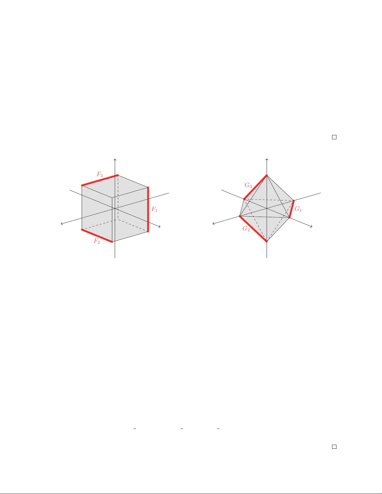
On the Uniqueness of F r ´ ec het Means for P olytope Norms Roan T albut 1 , : , Andrew McCormac k 2 , and An thea Mono d 1 1 Departmen t of Mathematics, Imp erial College London, UK 2 Departmen t of Mathematical and Statistical Sciences, Univ ersity of Alberta, Edmonton, Canada : Corresp onding e-mail: roan.s.talbut@durham.ac.uk Abstract F r ´ ec het means are a popular t yp e of a v erage for non-Euclidean datasets, defined as those points whic h minimise the av erage squared distance to a set of data p oints. W e consider the b eha viour of sample F r´ ec het means on normed spaces whose unit ball is a p olytope; this setting is rarely cov ered by existing literature on F r ´ ec het means, whic h focuses on smooth spaces or spaces with b ounded curv ature. W e study the geometry of the set of F r ´ ec het means o v er p olytope normed spaces, with a focus on dimension and probabilistic conditions for uniqueness. In particular, we provide a geometric characterisation of the threshold sample size at whic h F r ´ ec het means ha v e a positive probability of b eing unique, and we prov e that this threshold is at most one more than the dimension of our space. W e are able to use this geometric characterisation to compute the unique F r ´ ec het mean sample threshold in the case of the ℓ 8 and ℓ 1 norms. Keyw ords: p olytop e geometry , F r´ ec het means, p olytop e norms, uniqueness, small samples. 1 In tro duction The F r´ ec het mean set of a collection of data p oints in a metric space is defined as the set of p oin ts that minimise the a v erage squared distance to the data p oints (F r ´ ec het, 1948 ). F r ´ ec het means generalise the classical Euclidean notion of a mean to datasets taking v alues in general metric spaces. As this definition only uses the metric of the underlying state space, F r ´ ec het means hav e b een applied to a wide v ariet y of differen t geometric settings such as the space of PSD matrices (Arsigny et al. , 2007 ; Fiori, 2009 ; P etersen et al. , 2019 ), the space of p ersistence diagrams in top ological data analysis (Mileyko et al. , 2011 ; Cao & Mono d, 2022 ), and W asserstein space (Panaretos & Zemel, 2020b ; Panaretos et al. , 2020 ). Definition 1.1 giv es the formal definition of F r´ ec het means on a general metric space, for b oth p opulations and samples. Definition 1.1. Let X b e a random v ariable taking v alues in a general metric space p Ω , d q . Its p opulation F r ´ ec het function f : Ω Ñ R is defined as f p θ q “ E “ d p X, θ q 2 ‰ . F or a sample t x 1 , . . . , x n u Ă Ω, the sample F r ´ ec het function is defined as f p θ q “ 1 n n ÿ i “ 1 d p x i , θ q 2 . The (p opulation/sample) F r´ echet mean set is then the set of global minima: F “ argmin θ P Ω f p θ q . W e often denote these F r ´ ec het mean sets by F p X q or F p x 1 , . . . , x n q . In this pap er, we study the behaviour of sample F r´ echet means on normed spaces whose unit ball is a p olytope, hereafter referred to as spaces with a p olytop e norm . This fundamen tal setting is not cov ered b y most F r´ echet mean literature, which instead fo cuses on manifolds (Bhattachary a & Patrangenaru, 2003 , 2005 ) or spaces with bounded curv ature (Sturm, 2003 ; Am´ endola & Mono d, 2024 ). Despite this, polytop e norms are prev alen t in statistics; the ℓ 1 norm is used in LASSO regression (Ranstam & Co ok, 2018 ) in order to encourage sparse parameterisation of regression mo dels, and av oid ov erfitting to data. Our work directly addresses ℓ 1 F r ´ ec het means, as w e show with running examples throughout this pap er. How ev er, our results are far more general, and apply to F r´ echet means induced by any p olytop e norm. W e also present examples using the ℓ 8 norm to sho w the contrast in their b eha viour. F r ´ ec het means are defined as the solution set of an optimisation problem, so the question of existence and uniqueness is the natural first topic of study in an y geometric setting. The existence of a F r´ ec het mean is equiv alen t to a distribution ha ving finite moments, while the uniqueness of F r´ echet means is more heavily dep enden t on the underlying geometry . Sturm ( 2003 ) show ed that F r ´ ec het means are unique in spaces with non-p ositiv e Alexandro v curv ature, suc h as the cone of SPD matrices (Arsign y et al. , 2007 ), and the BHV space of phylogenetic trees (Billera et al. , 2001 ; Nye et al. , 2017 ). F or Riemannian manifolds, Bhattachary a & Patrangenaru ( 2003 ) give sufficient conditions for uniqueness of sample and p opulation F r´ echet means, and more recently it was shown that for any absolutely contin uous distribution ov er a complete Riemannian manifold, sample F r ´ ec het means will almost surely b e unique (Arnaudon & Miclo, 2014 ). In this paper, we presen t similarly foundational results on the uniqueness of F r´ ec het means from polytop e norms. F or data with an absolutely contin uous underlying distribution, we sho w that the p opulation F r´ echet mean will b e unique, while the probability of a unique sample F r´ echet mean will conv erge to one. W e then consider the probabilit y of a unique F r´ echet mean for small samples; we show that there is some sample threshold below whic h F r´ echet means are almost nev er unique, and ab ov e which F r´ echet means hav e a positive probabilit y of uniqueness. This result follo ws from c haracterising the geometric configurations which can o ccur with positive probabilit y; Durier & Mic helot ( 1985 ) tak e a similar view in their study of F ermat–W eb er p oin ts, though their w ork is deterministic where ours is probabilistic. W e show that this sample threshold is at most k ` 1 for general p olytop e norms, where k is the dimension of our space. In the cases of the ℓ 8 and ℓ 1 norms, this threshold is k and 3 resp ectively . W e provide a brief in troduction to the relev an t p olytop e geometry in Section 2 and the geometric foun- dations of F r´ ec het means on norm spaces in Section 3 . W e will sho w that for any absolutely con tin uous distribution, the population F r´ echet mean will be unique, while th e probabilit y of a unique sample F r´ ec het mean is zero for small sample sizes and conv erging to one as the sample size increases ( Section 4 ). Our main result, Theorem 5.10 , gives geometric conditions whic h dictate the num ber of samples required for this probabilit y of uniqueness to go from zero to positive ( Section 5 ). In Section 6 , we present the threshold v alues for sp ecific norms. W e conclude by showing how the F rank–W olfe algorithm (F rank et al. , 1956 ) can b e used for the exact computation of F r´ echet means in Section 7 . Notation. W e use relint p U q , Cl p U q and aff p U q to denote the relative interior, closure and affine span of a set U Ď R k resp ectiv ely . W e use r k s to denote the set t 1 , . . . , k u . W e use e i to denote the standard i th basis v ecotr. Throughout this pap er f will refer to the sample F r´ echet function unless otherwise sp ecified. 2 P olytop e Geometry In this section, w e review the definitions of p olytop es, their faces and their polars. F or a more detailed in tro duction, we refer the reader to Ziegler ( 2012 ). W e then formalise a p olytop e norm — a norm whose unit ball is a p olytope — and review the conv ex geometry corresp onding to such a norm. 2.1 P olytop es P olytop es can b e viewed in tw o wa ys — as a conv ex h ull of finitely many points, or an intersection of finitely man y halfspaces. Definition 2.1 (P olytop e) . A polytop e Q in R k is the con vex h ull of a finite set of points t v 1 , . . . , v r u Ă R k : Q “ con v pt v 1 , . . . , v r uq “ # r ÿ i “ 1 λ i v i : λ 1 , . . . , λ r ě 0 , r ÿ i “ 1 λ i “ 1 + . 2 (a) 2-dimensional hypercub e (b) 2-dimensional cross-p olytope x y z (c) 3-dimensional hypercub e x y z (d) 3-dimensional cross-p olytope Figure 1: The hypercub es and cross-p olytop es in dimension 2 and 3. Equiv alen tly , giv en a matrix A P R r ˆ k and a vector b P R r , a polytop e can also be defined as the set of all solutions to the follo wing linear inequalities: Q “ P p A, b q : “ ␣ x P R k | A x ď b , co ordinatewise ( , where it is assumed that the set of solutions is a bounded set. The conv ex h ull and inequalit y represen tations of Q are referred to as the v ertex and halfspace representations resp ectiv ely . Throughout this paper, w e use t w o classes of p olytop es as running examples; these are h ypercub es and cross-p olytopes, which arise as the unit balls of the ℓ 8 and ℓ 1 norms resp ectively . The vertex and halfspace represen tation of each of these balls is given in Examples 2.2 and 2.3 , while Figure 1 shows visualisations of these p olytopes for k “ 2 and 3. Example 2.2 (Hypercub es) . W e define the k -dimensional hypercub e B k 8 b y B k 8 : “ con v ` t´ 1 , 1 u k ˘ “ t x P R k : @ i P r k s , | x i | ď 1 u . Example 2.3 (Cross-polytop es) . W e define the k -dimensional cross-p olytop e B k 1 b y B k 1 : “ con v pt˘ e 1 , . . . , ˘ e k uq “ t x P R k : ř k i “ 1 | x i | ď 1 u . An imp ortan t attribute of the geometry of a p olytope is its facial structure. Definition 2.4 (F ace, face lattice) . Let c P R k , c 0 P R be suc h that c ⊺ x ď c 0 for all x in the p olytop e Q . A face F of Q is an intersection of the form: F “ Q č t x P R k : c ⊺ x “ c 0 u . The set of all faces is denoted F p Q q , and forms a lattice with the partial ordering given by inclusion. W e note that a polytop e Q is a face of itself, as is the empty set; an y other face of Q is referred to as a pr op er face of Q . The 0-dimensional faces of a polytop e are called v ertices, the 1-dimensional faces of a p olytope are edges, and the maximal prop er faces of Q are fac ets . When Q is giv en by con v t v 1 , . . . , v r u , ev ery face of Q will b e given by the conv ex h ull of some subset of t v 1 , . . . , v r u . When Q is given by solutions to a collection of linear inequalities, every face of Q is the solution set of the same inequalities, with some tak en to b e equalities. Lastly , w e introduce the p olar of a p olytop e whic h is intimately tied to subgradients of p olytope norms. 3 Definition 2.5 (Polar P olytope) . Let Q “ conv t v 1 , . . . , v r u Ă R k b e a full-dimensional p olytop e con taining the origin in its in terior. The p olar of Q is the p olytop e given by: Q ∆ : “ t x P R k : @ y P Q, y ⊺ x ď 1 u “ P p V , 1 q , where V is the matrix with rows v 1 , . . . , v r . The faces of Q ∆ are giv en by t F 3 : F P F p Q qu , where F 3 : “ t x P Q ∆ : @ y P F , y ⊺ x “ 1 u . W e call F 3 the p olar of the face F . The faces of a p olytop e are in bijection with the faces of its p olar p olytop e, in fact their face lattices are an ti-isomorphic; F 3 1 Ď F 3 2 if and only if F 2 Ď F 1 . The p olar of a p olar p olytope Q ∆∆ is equal to Q , and as suc h, we see that the p olar of P p A, 1 q is given by the conv ex hull of the row vectors of A . Example 2.6 (Hypercub es and Cross-p olytop es) . The k -dimensional h yp ercube and cross-polytop e are polars of eac h other. The p olars of the hypercub e vertices are the facets of the cross-p olytop e, and vice v ersa. 2.2 P olytop e Norms W e no w review the con v ex analysis of a norm whose unit ball is a p olytop e B . When defining p olytop e norms, the h yp erplane represen tation is most natural. Definition 2.7 (P olytope Normed Space) . Let B “ P p A, 1 q Ă R k b e a full-dimensional, cen trally symmetric p olytope, meaning that x P B if and only if ´ x P B . Then p R k , } ¨ } B q is a p olytop e normed space where the B -norm is defined by } x } B : “ inf t d P R ą 0 : d ´ 1 x P B u ” max i Pr r s p A x q i . (1) The metric induced b y the B -norm is denoted by d B . It is straigh tforw ard to show that } x } B is a norm, and that the unit ball of } ¨ } B is the polytop e B . In the case of our standard p olytope examples: • The hypercub e B k 8 giv es rise to the ℓ 8 norm } x } B k 8 ” } x } 8 “ max i Pr k s t | x i |u . • The cross-p olytop e B k 1 giv es rise to the ℓ 1 norm } x } B k 1 ” } x } 1 “ ř i Pr k s | x i | . T o discuss the lo cal b eha viour of a p olytope norm near x , we need to kno w which rows of A are ac- tiv e, meaning that they attain the comp onen twise maxim um of A x . W e refer to these rows as the active c onstr aints . In the following definition, we write a P A to mean a is a row vector of A . Definition 2.8. Let F b e a prop er face of B . The active constraints on F , denoted by A p F q , is the set: A p F q “ t a P A : for all x P F , a ⊺ x “ 1 u . Similarly , for an y x P R k w e define A p x q to b e the activ e constraints of } x } B . That is: A p x q “ t a P A : a ⊺ x “ } x } B u . Notice that conv A p F q “ F 3 . W e also note that the set of op en cones generated by prop er faces of B , relint p R ` F q , partition R k zt 0 u according to the active constraints; x P relin t p R ` F q if and only if A p x q “ A p F q . This partition of the space is the fac e fan of B . Finally , w e review the subgradient and directional deriv ativ es of the B -norm at x . Definition 2.9 (Subgradien t, Directional Deriv ative) . The subgradient of a conv ex function g : R k Ñ R at x is given by: B g p x q : “ t v : g p z q ě g p x q ` v ⊺ p z ´ x q for all z P R k u . The directional deriv ativ e in direction t P R k , denoted b y B t g p x q , is B t g p x q : “ lim h Ñ 0 ` h ´ 1 p g p x ` h t q ´ g p x qq “ sup v PB g p x q v ⊺ t . This equalit y is from Theorem 23.4 of (Ro c k afellar, 1970 ). 4 R emark 2.10 . The subgradient of a maxim um of differentiable functions g p x q “ max t g 1 p x q , . . . , g n p x qu is kno wn to b e the con vex h ull of the gradients of active functions at x : B g p x q “ conv t ∇ x g i p x q : g i p x q “ g p x qu . Applying this result to a p olytope B -norm, which is a maximum of linear functions by ( 1 ), we obtain that B} x } 2 B “ con v ␣ ∇ x p a J x q 2 : a P F 3 ( “ 2 } x } F 3 , when x P relint p R ` F q . Consequen tly , the subgradien t of the sample F r´ echet function will b e giv en b y B f p x q “ 2 ř i Pr n s } x i ´ θ } F 3 i , where F i is the unique face such that x i ´ θ P relint p R ` F i q , and the summation is a Minko wski sum. Since a con vex function is minimized if and only if its subgradient con tains 0 , it follows that θ is a sample F r´ ec het mean if and only if 0 P ř i Pr n s } x i ´ θ } F 3 i . 3 F r ´ ec het Means on Normed Spaces In this section, w e discuss F r´ echet means and outline their fundamental prop erties in the case of (p olytop e) normed spaces. All F r´ ec het means in the sections to follow are taken with resp ect to a given B -norm, unless stated otherwise. As defined in Definition 1.1 , we use f to denote a F r´ echet function; this is given b y f p θ q “ E r d p X , θ q 2 s for general random v ariables and f p θ q “ n ´ 1 ř n i “ 1 d p x i , θ q 2 for a sample t x 1 , . . . , x n u . W e then denote the F r´ echet mean set b y F : “ argmin θ f p θ q , which w e ma y abbreviate to F p X q or F p x 1 , . . . , x n q . Understanding the conv exit y of the F r´ echet function is crucial for understanding the existence and con- v exity of F r´ echet mean sets; these foundational conv exit y results hav e b een established in man y settings, such as W asserstein spaces (P anaretos & Zemel, 2020a ), Riemannian spaces (Afsari, 2011 ), metric trees, (Romon & Brunel, 2023 ), and the tropical pro jectiv e torus (Lin et al. , 2025 ). Belo w, w e state the conv exit y results w e require in the case of a general normed space. These results b elow are generalisations of the con v exit y results established in the tropical setting by Lin et al. ( 2025 ), and mirror the w ork of (Durier & Mic helot, 1985 ) on F ermat–W eb er p oints. Lemma 3.1. Fix a norme d sp ac e p R k , } ¨ } q with induc e d metric d . F or al l x , d p¨ , x q 2 is c onvex, and in fact if, for some t P p 0 , 1 q we have d pp 1 ´ t q θ 1 ` tθ 2 , x q 2 “ p 1 ´ t q d p θ 1 , x q 2 ` td p θ 2 , x q 2 , then d p θ 1 , x q “ d p θ 2 , x q . The F r´ echet function is also c onvex, and so F r´ echet me an sets ar e c onvex. Pr o of. Conv exit y of a squared norm is immediate from the con v exity of norms, as the function y ÞÑ y 2 is strictly monotone increasing and strictly con vex ov er the domain R ě 0 : }p 1 ´ t q θ 1 ` tθ 2 ´ x } 2 ď pp 1 ´ t q} θ 1 ´ x } ` t } θ 2 ´ x }q 2 , ď p 1 ´ t q} θ 1 ´ x } 2 ` t } θ 2 ´ x } 2 . Hence } θ ´ x } 2 “ d p θ , x q 2 is strictly con vex in θ . The second statement follo ws from the strict conv exit y of y ÞÑ y 2 ; w e hav e equality if and only if } θ 1 ´ x } 2 “ } θ 2 ´ x } 2 . The con v exity of the F r´ echet function f is a direct result of exp ectation preserving conv exit y , while the con vexit y of F r´ echet mean sets follows from the conv exit y of f . Building on Lemma 3.1 , we will see that F r´ echet mean sets are given by intersections of spheres. Lemma 3.2 expresses this in the case of a general p opulation X „ P , while Corollary 3.3 considers the case of a finite sample. Lemma 3.2. L et X „ P b e a r andom variable in p R k , } ¨ }q . Assume that θ 1 and θ 2 ar e F r´ echet me ans of X . Then for every x in the esssupp p P q , we have d p x , θ 1 q “ d p x , θ 2 q . Pr o of. Fix some x P esssupp p P q . By definition, for all m P N w e ha v e P p B 1 { m p x qq ą 0. W e will sho w that there is some x m P B 1 { m p x q such that d p x m , θ 1 q “ d p x m , θ 2 q by contradiction. Let θ 3 “ 1 2 p θ 1 ` θ 2 q b e a midp oin t of θ 1 , θ 2 . By the con vexit y of d p X , ¨q and strict conv exit y of y ÞÑ y 2 : d p X, θ 3 q 2 ď ` 1 2 d p X, θ 1 q ` 1 2 d p X, θ 2 q ˘ 2 ď 1 2 ` d p X, θ 1 q 2 ` d p X , θ 2 q 2 ˘ . 5 W e assume for all u P B 1 { m p x q , d p u , θ 1 q ‰ d p u , θ 2 q , so the ab o v e inequality is strict. It follo ws that E “ I X P B 1 { m d p X, θ 3 q 2 ‰ ă 1 2 ` E “ I X P B 1 { m d p X, θ 1 q 2 ‰ ` E “ I X P B 1 { m d p X, θ 2 q 2 ‰˘ . Hence E “ d p X, θ 3 q 2 ‰ ă 1 2 ` E “ d p X, θ 1 q 2 ‰ ` E “ d p X, θ 2 q 2 ‰˘ , whic h con tradicts the optimality of θ 1 and θ 2 . Therefore for all m P N , we can pick some x m P B 1 { m p x q such that d p x m , θ 1 q “ d p x m , θ 2 q . B y contin uit y of the distance function we conclude d p x , θ 1 q “ d p x , θ 2 q . As a natural corollary to Lemma 3.2 , w e see that an y distribution whose essen tial support is R k m ust ha v e a unique F r´ ec het mean ( Theorem 4.1 ). Ho w ever, for finite samples, uniqueness is not guaranteed. F r´ ec het means are given by intersections of spheres cen tred at each data p oin t, as shown in Corollary 3.3 . In fact, in the case of p olytop e norms, F r´ echet means are intersections of faces. Figure 2 provides a visualisation of this b eha viour for F r ´ ec het mean sets of a small num ber of samples. Corollary 3.3. Fix a norme d sp ac e p R k , } ¨ } B q with unit b al l B . Ther e exist unique d i P R ě 0 such that F p x 1 , . . . , x n q “ č i Pr n s t d i B ` x i u “ č i Pr n s t d i B B ` x i u , wher e B B is the b oundary of B . In p articular, if B is a p olytop e then F p x 1 , . . . , x n q is a p olytop e. Mor e over, for every i P r n s ther e exists a pr op er fac e F i of B such that F is given by Ş i Pr n s t d i F i ` x i u . Pr o of. By Lemma 3.2 , the distances d i “ d p x i , θ q are fixed for all θ P F p x 1 , . . . , x n q . Hence : F p x 1 , . . . , x n q Ď č i Pr n s t d i B B ` x i u Ď č i Pr n s t d i B ` x i u Ď F p x 1 , . . . , x n q . This follows from Lemma 3.2 , nested in tersections, and the definition of the d i . When B is a polytop e, the in tersection of balls ab out eac h x i is also a p olytope. W e prov e the last claim by con tradiction. Suppose there is no constrain t a P A whic h is active for all t x i ´ θ : θ P F u . Then for all a j P A , we hav e some θ 1 , . . . , θ r P F such that a j P A is not in A p x i ´ θ j q . By the con vexit y of F , 1 r ř j Pr r s θ j is a F r ´ ec het mean and must b e in the set d i B B ` x i . F or all a j , w e hav e a ⊺ j p x i ´ θ j q ă } x i ´ θ j } B “ d i , a ⊺ j p x i ´ θ k q ď } x i ´ θ k } B “ d i . W e obtain that › › › x i ´ 1 r ř j Pr r s θ j › › › B “ max j 1 a J j 1 ´ 1 r ř j Pr r s p x i ´ θ j q ¯ ă 1 r ř j Pr r s } x i ´ θ j } B “ d i , con tradicting 1 r ř j Pr r s θ j P F . So for all x i , there is some face F i of B with F Ď d i F i ` x i . Hence : F p x 1 , . . . , x n q Ď č i Pr n s t d i F i ` x i u Ď č i Pr n s t d i B B ` x i u “ F p x 1 , . . . , x n q . So the result is pro ved. W e ha ve prov ed a more general result in the final part of this corollary , which will b e useful later: Corollary 3.4. Supp ose S is a c onvex set c ontaine d in a p olytop e Q . If S and relin t Q ar e disjoint, then S is c ontaine d in some pr op er fac e of Q . R emark 3.5 . Corollary 3.3 highligh ts why F r´ ec het means with resp ect to polytop e balls are particularly in teresting to study , as such balls often ha v e intersections that are positive dimensional, as is illustrated in the left hand side of Figure 2 . By con trast, the F r´ echet mean of tw o p oints x 1 , x 2 with respect to a norm with a strictly con v ex ball will alwa ys be the unique point where the balls around x 1 and x 2 ha ve a single con tact p oin t with each other. 6 x 1 “ p 0 , 0 q x 2 “ p 2 , 1 q x 1 “ p´ 4 , ´ 4 q x 2 “ p 1 , 2 q x 3 “ p 2 , ´ 1 q Figure 2: F r´ ec het mean sets (red) are contained in faces of balls that are centred ab out each data p oint ( Corollary 3.3 ). W e conclude with a final corollary on F r ´ ec het means for normed spaces with strictly conv ex balls, to sho w the contrast with the p olytop e norm setting; if the unit ball of a norm is strictly conv ex, then F r´ ec het means m ust b e unique. Corollary 3.6. If B is a strictly c onvex b al l, in the sense that the r elative interior of any line b etwe en two p oints in B B is c ontaine d in int p B q , then F p x 1 , . . . , x n q c onsists of a single p oint. In p articular, sample F r´ echet me ans with r esp e ct to ℓ p norms, p P p 1 , 8q , ar e always unique. Pr o of. The norm of a strictly con v ex ball has the prop erty that whenev er x is not prop ortional to y with resp ect to a non-negative scaling, we hav e for all t P p 0 , 1 q that }p 1 ´ t q x ` t y } B “ ` p 1 ´ t q} x } B ` t } y } B ˘ › › › › p 1 ´ t q} x } B p 1 ´ t q} x } B ` t } y } B x } x } B ` t } y } B p 1 ´ t q} x } B ` t } y } B y } y } B › › › › B ă p 1 ´ t q} x } B ` t } y } B , since the ab o v e expression is a conv ex com bination of the points x {} x } B , y {} y } B P B B . Consider tw o F r ´ ec het means, θ 1 , θ 2 P F p x 1 , . . . , x n q . By the conv exit y of F , and Lemma 3.2 , p 1 ´ t q θ 1 ` tθ 2 has the same distance to x 1 as θ 1 and θ 2 . So by the result ab o ve we must hav e that x 1 ´ θ 1 “ c p x 1 ´ θ 2 q for some c ě 0, as well as d p x 1 , θ 1 q “ d p x 1 , θ 2 q . The only w ay this can o ccur is if c “ 1, and thus θ 1 “ θ 2 . The ℓ p balls are strictly con vex for p P p 1 , 8q since if } x } p “ } y } p “ 1 with x ‰ y , then }p 1 ´ t q x ` t y } p p “ ř k i “ 1 |p 1 ´ t q x i ` ty i | p ď ř k i “ 1 pp 1 ´ t q| x i | ` t | y i |q p ă ř k i “ 1 ` p 1 ´ t q| x i | p ` t | y i | p ˘ “ 1 . The strict inequalit y follows from Jensen’s inequality and the fact that x ‰ y . 4 Large Sample Uniqueness W e contin ue our study of p olytop e F r´ echet means by determining the probability that a sample F r´ echet mean is unique, assuming that distribution of the samples has a positive density on R k with resp ect to the Leb esgue measure. Theorem 4.1. Supp ose X „ P , with esssupp p P q “ R k . Then F p X q is unique. Pr o of. This follows directly from Lemma 3.2 . As sho wn b y Bhattac harya & Patrangenaru ( 2003 ), sample F r´ echet means are strongly consistent esti- mators for p opulation F r´ echet means. 7 Theorem 4.2. L et t X i u i P N b e a se quenc e of i.i.d. r andom ve ctors with X i „ P , wher e P has a unique p opulation F r´ echet me an θ ˚ . L et θ n b e a r andom variable such that θ n P F p X 1 , . . . , X n q almost sur ely. Then θ n c onver ges almost sur ely to θ ˚ . Pr o of. This is a direct application of Theorem 2.3 of (Bhattac hary a & P atrangenaru, 2003 ). W e note that closed and b ounded subsets of R k are compact, and w e ha ve assumed the population F r´ echet function is finite. W e ha v e also assumed that P has a unique F r´ echet mean θ ˚ . Then b y Theorem 2.3 of Bhattac hary a & P atrangenaru ( 2003 ), θ n is a strongly consisten t estimator for θ ˚ . The consistency of sample F r´ echet means do es not guarantee their uniqueness. In Theorem 4.3 , we show that the probabilit y of a unique sample F r´ ec het mean tends to one as the sample size increases. Theorem 4.3. Supp ose X „ P , with esssupp p P q “ R k . L et p n b e t he pr ob ability that F p X 1 , . . . , X n q c onsists of a single element. Then p n c onver ges to 1 as n Ñ 8 . Pr o of. Supp ose that there is some sample F r´ echet mean θ P F p X 1 , . . . , X n q such that for every p ossible activ e constraint a i P A , there is some data p oint X j p i q satisfying A p X j p i q ´ θ q “ a i . Then by Corollary 3.3 , the F r´ echet mean set is con tained in the intersection of corresp onding faces, Ş i } θ ´ X j p i q } F i ` X j p i q and so F p X 1 , . . . , X n q Ď t x : a ⊺ i p x ´ X j p i q q “ } θ ´ X j p i q }u . (2) As the set of all a i spans R k , the linear constrain ts in 2 define a unique point in F p X 1 , . . . , X n q . It now suffices to sho w that, with probabilit y tending to 1, there is some F r´ ec het mean θ such that A “ t A p X j ´ θ q , j “ 1 , . . . , n u . F or each facet F i , consider the intersection S i “ Ş θ P B 1 p θ ˚ q p θ ´ relin t p R ` F i qq Ă R k (see Figure 3 ). This is the set of p oin ts x with A p x ´ θ q “ a i for all θ in the unit ball ab out θ ˚ . This intersection is full dimensional, so P p X j P S i q “ c i ą 0. Let b n b e the probabilit y that there is some θ P F p X 1 , . . . , X n q in B 1 p θ ˚ q . By the argumen t ab o ve, we can b ound p n b elo w using b n , c i : p n ě P p A “ t A p X j ´ θ q , j “ 1 , . . . , n uq ě P ptH ‰ F p X 1 , . . . , X n q X B 1 p θ ˚ qu X t@ C i , H ‰ C i X t X 1 , . . . , X n uuq ě 1 ´ p 1 ´ b n q ´ ř i Pr r s p 1 ´ c i q n By the consistency of θ n ( Theorem 4.2 ), b n Ñ 1. So this lo w er b ound conv erges to 1. 1 θ ˚ θ n S 2 S 1 S 3 S 4 X j p 2 q X j p 4 q X j p 3 q X j p 1 q Figure 3: A visualisation of the cones S i (defined in the proof of Theorem 4.3 ) in the case of the ℓ 1 norm, and a sample such that every cone contains some data p oin t. As each cone contains a data p oint, whenever there is a F r ´ ec het mean within the unit ball of θ ˚ , it m ust b e a unique F r ´ ec het mean. 8 W e hav e shown that the probabilit y of uniqueness conv erges to one, now w e argue that it will never b e exactly one. This is b est seen by considering a sample close to a line a R for some a P A , such that w e hav e A p X j 1 ´ X j 2 q “ a or ´ a for all j 1 ‰ j 2 ď n ; suc h a sample will o ccur with p ositive probabilit y . F or such a sample, the F r´ echet mean set is a p k ´ 1 q dimensional p olytop e contained in the hyperplane t x : a ⊺ x “ n ´ 1 ř j ď n a ⊺ X j u , and so is not unique. Figure 4 shows an example of this using the ℓ 8 -norm. X 1 “ p 0 , 0 q X 3 “ p´ 4 , 1 q X 4 “ p 8 , ´ 1 q X 2 “ p 4 , 2 q Figure 4: A data configuration whic h occurs with p ositive probabilit y and has non-unique ℓ 8 F r ´ ec het means. R emark 4.4 . The probability of uniqueness is alwa ys zero for samples of size 2. With probability 1, X 2 is in X 1 ` relint R ` F for some facet F of B . In this case, the F r´ ec het mean set F is a k ´ 1 dimensional p olytop e con tained in the hyperplane t x : a ⊺ x “ a ⊺ p X 1 ` X 2 q{ 2 u where a is the normal vector of the facet F . W e’v e v erified that the population F r´ ec het mean is unique for positive densit y distributions. W e hav e also used the consistency of sample F r´ ec het means to deduce that the probabilit y of a sample ha ving a unique F r ´ ec het mean con v erges to 1 (but nev er equals 1) as our sample size increases. In the follo wing subsection, w e study the uniqueness b eha viour of F r´ ec het means for small samples. 5 Sample Threshold for Unique F r ´ ec het Means In this section, w e identify the com binatorial conditions that dictate the sample size needed for the sample F r ´ ec het mean to b e unique with p ositive probabilit y . W e sho w that this sample size is a threshold in that there is some v alue N p B q suc h that the probability of a unique F r´ ec het mean is p ositive for a sample of size n if and only if n ě N p B q . F or the ℓ 1 norm, this sample threshold is just 3, but for the ℓ 8 norm, this sample threshold is equal to the dimension of the space, k . T o understand the dimension of F r ´ ec het mean sets, w e study which faces of balls centred ab out our data p oin ts can be intersected to define the F r´ echet mean set ( Corollary 3.3 ). The dimension of the F r´ echet mean set F is iden tifiable from the minimal faces whose intersection is the F r´ echet mean set. W e call these minimal faces the fac e typ e of a sample. W e sho w that the face type of a sample is almost surely well-defined and determines the dimension of F , then w e identify which face t yp es o ccur with p ositive probability b y considering subgradien ts. T o define the face type of a sample, w e will assume that no data p oint is also a F r ´ ec het mean of the sample, which is true almost surely . Lemma 5.1. If esssupp p P q “ R k then with pr ob ability one, the r andom sample p oints X 1 , . . . , X n i.i.d. „ P ar e not F r ´ echet me ans of the ful l sample; for al l i , X i R F p X 1 , . . . , X n q . Pr o of. W e claim X 1 is a F r´ ec het mean of X 1 , . . . , X n iff X 1 is a F r´ ec het mean of X 2 , . . . , X n . Denote the F r ´ ec het function for the sample X 1 , . . . , X n as f p x q , and the F r ´ ec het function for X 2 , . . . , X n as f ˆ 1 p x q , so: f p x q “ n ´ 1 n ÿ i “ 1 d p X i , x q , f ˆ 1 p x q “ p n ´ 1 q ´ 1 n ÿ i “ 2 d p X i , x q . 9 The subgradien t of d p X 1 , ¨q 2 at X 1 is 0, so b y Theorem 23.8 in Ro c k afellar ( 1970 ): n B f p X 1 q “ p n ´ 1 qB f ˆ 1 p X 1 q . The p oint X 1 is a F r´ echet mean of X 1 , . . . , X n if and only if 0 P B f p X 1 q , and is a F r´ echet mean of X 2 , . . . X n if and only if 0 P B f ˆ 1 p X 1 q . These conditions are equiv alen t, so our claim is prov ed. W e now show that the sample p oints X 1 , . . . , X n are almost never F r´ echet means of the full sample X 1 , . . . , X n . Let A 1 b e the even t that X 1 is a F r´ echet mean of the full sample, or equiv alen tly X 1 P F p X 2 , . . . , X n q . By Corollary 3.3 , the set F p X 2 , . . . , X n q has co-dimension ě 1, and hence has P -measure zero. Therefore P p A 1 q “ 0. W e can define A 2 , . . . , A n similarly , and by taking a union ov er A 1 , . . . , A n w e conclude that the F r ´ ec het mean set intersects the sample X 1 , . . . , X n with probabilit y zero. 5.1 F ace Types As sho wn in Corollary 3.3 , the F r´ ec het mean set is an in tersection of faces of balls cen tred at eac h data point. W e will define the face type of a sample as the minimal sequence of faces of balls where the F r´ echet mean set is their in tersection. The lemma b elo w ensures this is almost surely well-defined. Lemma 5.2. L et X 1 , . . . , X n b e a finite sample with F r´ echet me an set F such that X i R F for every i . L et d i “ d B p X i , F q . Then the set of tuples of fac es S F p X 1 , . . . , X n q “ " p F 1 1 , . . . , F 1 n q : Ş n i “ 1 p X i ´ d i F 1 i q “ F * Ď F p B q n has a le ast element p F 1 , . . . , F n q P S F with r esp e ct to c o or dinate-wise c ontainment. Pr o of. By Corollary 3.3 , S F p X 1 , . . . , X n q is not empty . Define p F 1 , . . . , F n q by F i “ Ş p F 1 1 ,...,F 1 n qP S F F 1 i . Then for all p F 1 1 , . . . , F 1 n q P S F p X 1 , . . . , X n q w e hav e that p F 1 , . . . , F n q ď p F 1 1 , . . . , F 1 n q . It suffices to sho w that p F 1 , . . . , F n q P S F p X 1 , . . . , X n q . This follo ws from: Ş n i “ 1 p X i ´ d i F i q “ Ş n i “ 1 ˆ X i ´ d i ` Ş p F 1 1 ,...,F 1 n qP S F F 1 i ˘ ˙ “ Ş p F 1 1 ,...,F 1 n qP S F Ş n i “ 1 p X i ´ d i F 1 i q “ Ş p F 1 1 ,...,F 1 n qP S F F “ F . Using the lemma ab o v e, we can define the face type of a sample: Definition 5.3 (F ace Type) . Consider a sample X 1 , . . . , X n suc h that no data point is a F r´ echet mean of the full dataset. Suc h a sample is defined to hav e face type p F 1 , . . . , F n q ab out the F r ´ ec het mean set F when p F 1 , . . . , F n q is the least elemen t of S F p X 1 , . . . , X n q . By Lemma 5.1 and Lemma 5.2 , the face type of a sample is w ell-defined almost surely . How ev er, we will use a more geometric description of face type through the rest of this section. Both here and throughout the rest of this section w e use d i : “ d B p X i , F q which is well-defined by Corollary 3.3 . Lemma 5.4. L et X 1 , . . . , X n b e a sample with fac e typ e p F 1 , . . . F n q and d i “ d B p X i , F q . Then we have that relin t F “ Ş n i “ 1 relin t p X i ´ d i F i q . A sample has fac e typ e p F 1 , . . . , F n q if and only if ther e is some θ P relint F such that for al l i P r n s , X i ´ θ P relint p R ` F i q . Pr o of. By definition, F Ď p X 1 ´ d 1 F 1 q . Suppose that relint F do es not intersect relin t p X 1 ´ d 1 F 1 q , so relin t F Ď p X 1 ´ d 1 B F 1 q . By Corollary 3.4 , there is some face F 1 1 of F 1 satisfying F Ď X 1 ´ d 1 F 1 1 . Hence p F 1 1 , F 2 , . . . , F n q P S F p X 1 , . . . , X n q , contradicting the definition of p F 1 , . . . , F n q . Therefore (for any i , by symmetry) relin t F in tersects relint p X i ´ d i F i q , and b y (Ro c k afellar, 1970 , Theorem 6.5): relin t p F Xp X i ´ d i F i qq “ relin t F X relint p X i ´ d i F i q , relin t F Ď relint p X i ´ d i F i q . 10 Applying (Ro c k afellar, 1970 , Theorem 6.5) again to X 1 ´ d 1 F 1 , . . . , X n ´ d n F n : relin t F “ Ş n i “ 1 relin t p X i ´ d i F i q . Supp ose our sample has face type F 1 , . . . , F n . Then for all θ P relint F , we ha v e θ P relint p X i ´ d i F i q and therefore X i ´ θ P relint R ` F i . T o show the conv erse, consider θ P relint F such that for all i , X i ´ θ P relint p R ` F i q . W e define d i “ d B p X i , θ q . Assume that p X 1 , . . . , X n q has the face type F 1 1 , . . . , F 1 n . Then by the argument ab ov e, θ P relin t p X i ´ d i F 1 i q , implying that X i ´ θ P d i relin t F 1 i Ď relin t p R ` F 1 i q . The fans t relint p R ` F q : F P F p B qu partition R k zt 0 u , so it m ust b e the case that F 1 i “ F i and our sample has t yp e p F 1 , . . . , F n q . As the relativ e interior of the F r´ echet mean set is the intersection of the relativ e interiors of the faces X i ´ d i F i , w e can deduce the dimension of F from the face type of the sample. Lemma 5.5. If W 1 , . . . , W m ar e r elatively op en and Ş m i “ 1 W i ‰ H , then Ş m i “ 1 aff p W i q “ aff p Ş m i “ 1 W i q . Pr o of. It suffices to consider the m “ 2 case. The space aff p W 1 q X aff p W 2 q is affine and contains W 1 X W 2 , so w e get that aff p W 1 X W 2 q Ď aff p W 1 q X aff p W 2 q . No w fix y P aff p W 1 q X aff p W 2 q , x P W 1 X W 2 . As W 1 , W 2 are relativ ely op en, there exists some ϵ ą 0 suc h that p 1 ´ ϵ q x ` ϵ y P W 1 X W 2 . He nce y P aff pt x , p 1 ´ ϵ q x ` ϵ y uq Ď aff p W 1 X W 2 q . R emark 5.6 . The face type of a sample is undefined if and only if some data p oint X i is a F r´ echet mean of the full dataset. Lemma 3.2 tells us the F r´ echet mean is the unique p oint X i in this case, while Lemma 5.1 tells us this is a probability zero even t. F or the rest of this section we exclude this case, assuming that d i “ d B p X i , F q ą 0. 5.2 T yp e Ev en ts By Lemma 5.5 , w e can deduce the dimension of a F r´ echet mean set from the face type of a sample. W e must no w identify which face types o ccur with p ositive probabilit y , and identify whic h face types corresp ond to a unique F r´ echet mean. T o determine whic h face t yp es o ccur with p ositiv e probability , w e define the (lifted) t yp e ev ent. Through this section, we use C i and G i to denote R ` F i and F 3 i resp ectiv ely . Definition 5.7 ((Lifted) Type Even t) . Consider the random vector p X 1 , . . . , X n q P R nk . In this space, the typ e event U F 1 ,...,F n is giv en by: U F 1 ,...,F n “ tp X 1 , . . . , X n q P R nk : p X 1 , . . . , X n q has face t yp e p F 1 , . . . F n qu . Then w e define the lifte d typ e event as the set U F 1 ,...,F n , Θ “ tp X 1 , . . . , X n , θ q P R k p n ` 1 q : θ P relin t F , X i ´ θ P relint C i u , where C i denotes the cone R ` F i . Note that by Lemma 5.4 , the type even t is the image of the lifted type even t under the pro jection pro j : R k p n ` 1 q Ñ R kn giv en by p X 1 , . . . , X n , θ q ÞÑ p X 1 , . . . , X n q . Our goal is to classify the face t yp es p F 1 , . . . , F n q for which U F 1 ,...,F n has p ositiv e Leb esgue measure. Then as p X 1 , . . . , X n q has a p ositive densit y , suc h a face type o ccurs with p ositive probability . It is difficult to calculate the measure of the type even ts directly , so we will translate this condition into a linear relation on subgradien ts. F or this, w e define the zer o sub gr adient event . Definition 5.8 (Zero Subgradien t Even t) . The zero subgradient even t is given by: V F 1 ,...,F n , Θ “ ! p X 1 , . . . , X n , θ q P R k p n ` 1 q : 0 P relin t p ř n i “ 1 } X i ´ θ } G i q , X i ´ θ P relint C i ) , where G i denotes the p olar face F 3 i , and C i denotes the cone R ` F i . 11 Note that when w e ha v e X i ´ θ P relint C i for all i , the subgradien t of the F r´ ec het function is giv en b y B f p θ q “ ř n i “ 1 } X i ´ θ } G i . Hence, by the definition of subgradients, θ P F if and only if 0 P ř n i “ 1 } X i ´ θ } G i ( Remark 2.10 ). F rom this, we migh t hop e that the lifted type ev ent and the zero subgradient even t are equiv alen t, but this is not true. How ev er, they do coincide almost everywhere. Prop osition 5.9. The zer o sub gr adient event V F 1 ,...,F n , Θ is a r elatively op en p olyhe dr on; it is an interse ction of finitely many hyp erplanes and op en half sp ac es. F urthermor e, it c oincides with the lifte d typ e event everywher e other than on its b oundary: relin t V F 1 ,...,F n , Θ “ relin t U F 1 ,...,F n , Θ , Cl V F 1 ,...,F n , Θ “ Cl U F 1 ,...,F n , Θ . The pro of of this prop osition can b e found in Section A . 5.3 P olytop e Conditions for Unique F r´ ec het Means W e can now state and prov e the main result of this section ( Theorem 5.10 ), whic h establishes the conditions for U F 1 ,...,F n to o ccur with p ositiv e probability and to pro duce a unique F r´ echet mean. W e do this b y computing the dimension of the p olyhedron V F 1 ,...,F n , Θ , which then allo ws us to compute the dimension of pro j V F 1 ,...,F n , Θ and U F 1 ,...,F n . This result is crucial for not only computing the sample threshold for uniqueness, but also for pro ving that the sample threshold for uniqueness is well-defined. Theorem 5.10. The typ e event U F 1 ,...,F n and pro j V F 1 ,...,F n , Θ satisfy L p U F 1 ,...,F n q “ L p pro j V F 1 ,...,F n , Θ q . Ther efor e U F 1 ,...,F n has p ositive pr ob ability if and only if 0 P relin t ´ con v ´ Ť i Pr n s G i ¯¯ , (3) and ř i Pr n s dim G i “ dim ř i Pr n s aff G i . (4) The F r ´ echet me an of a sample in U F 1 ,...,F n is unique if and only if dim conv ´ Ť i Pr n s G i ¯ “ k . (5) T o understand this result, we return to one of our examples from Figure 2 , display ed again in Figure 5 , whic h shows a sample with face type p F 1 , F 2 , F 3 q “ p e 1 ` e 2 , conv t´ e 2 ˘ e 1 u , conv t´ e 1 ˘ e 2 uq . W e can test whether this face type satisfies the three conditions in Theorem 5.10 ; for this face type, note that p G 1 , G 2 , G 3 q “ p con v t e 1 , e 2 u , ´ e 2 , ´ e 1 q . The first condition (3) v erifies whether a sample can ha ve the face t yp e p F 1 , F 2 , F 3 q . This is sho wn to b e true in Figure 5 , and in fact con v ´ Ť i Pr n s G i ¯ “ con v t˘ e 1 , ˘ e 2 u whic h contains 0 in its relative interior. The second condition (4) verifies whether a sample has face type p F 1 , F 2 , F 3 q with p ositive probability . The dimensions of G 1 , G 2 , G 3 are 1,0,0 resp ectiv ely , while ř i ď 3 aff G i “ aff t´ e 1 , ´ e 2 u , which has dimension 1 “ 1 ` 0 ` 0. This v erifies that suc h a face t ype can o ccur with p ositiv e probabilit y; this configuration of data p oin ts around a F r ´ ec het mean is generic. Finally , the third condition (5) verifies whether having face t yp e p F 1 , . . . , F n q implies that our sample has a unique F r´ ec het mean. W e kno w that conv ´ Ť i Pr n s G i ¯ “ con v t˘ e 1 , ˘ e 2 u which has dimension 2, and therefore an y sample with this face type will hav e unique F r´ echet mean. W e pro ve Theorem 5.10 via the following three lemmas. Lemma 5.11. The zer o sub gr adient event V F 1 ,...,F n , Θ is non-empty if and only if 0 P relin t ´ con v ´ Ť i Pr n s G i ¯¯ . Pr o of. First, we hav e shown in the pro of of Prop osition 5.9 that V F 1 ,...,F n , Θ “ L ´ 1 F 1 ,...,F n p W q Ş Ş i Pr n s tp X 1 , . . . , X n , θ q : X i ´ θ P relint C i u , (6) where W is the relatively op en p olyhedral cone t w P R n ` : 0 P ř i Pr n s w i relin t G i u ( Lemma A.1 ). 12 x 1 “ p´ 4 , ´ 4 q x 2 “ p 1 , 2 q x 3 “ p 2 , ´ 1 q Figure 5: A sample with face type p F 1 , . . . , F n q “ p e 1 ` e 2 , conv t´ e 2 ˘ e 1 u , conv t´ e 1 ˘ e 2 uq , and its unique F r ´ ec het mean highlighted in red. W e will show that V F 1 ,...,F n , Θ is not empty if and only if W is non-empt y . Supp ose p X 1 , . . . , X n , θ q P V F 1 ,...,F n , Θ ; then b y (6) , W is non-empty . Conv ersely , supp ose w P W . Fix an arbitrary θ and pick some X i P θ ` w i relin t F i . By construction, X i ´ θ P relint C i and } X i ´ θ } B “ w i . By the definition of W we ha ve 0 P relint ´ ř i Pr n s } X i ´ θ } B G i ¯ , so p X 1 , . . . , X n , θ q P V F 1 ,...,F n , Θ . Next, note that (Rock afellar, 1970 , Theorem 6.9) states that for non-empt y con vex G 1 , . . . , G n Ă R k , then relin t ´ con v ´ Ť i Pr n s G i ¯¯ “ ď ! ř i Pr n s λ i relin t G i : λ i ą 0 , ř i Pr n s λ i “ 1 ) . (7) F rom this we see that 0 P relin t ´ con v ´ Ť i Pr n s G i ¯¯ if and only if W is non-empt y . W e conclude that V F 1 ,...,F n , Θ and V F 1 ,...,F n are non-empt y if and only if 0 P relint ´ con v ´ Ť i Pr n s G i ¯¯ . Lemma 5.12. The typ e event U F 1 ,...,F n has p ositive pr ob ability if and only if the p olyhe dr on pro j V F 1 ,...,F n , Θ has dimension nk . Pr o of. The zero subgradien t even t V F 1 ,...,F n , Θ is Borel measurable as it is a relatively op en p olyhedron. Consequen tly , pro j V F 1 ,...,F n , Θ is also a relativ ely op en p olyhedron and so also Borel measurable. W e also ha ve by Prop osition 5.9 and Theorem 6.6 of Ro c k afellar ( 1970 ): relin t U F 1 ,...,F n “ relin t p pro j U F 1 ,...,F n , Θ q “ pro j p relint U F 1 ,...,F n , Θ q “ pro j p relint V F 1 ,...,F n , Θ q “ relin t p pro j V F 1 ,...,F n , Θ q , U F 1 ,...,F n “ pro j U F 1 ,...,F n , Θ Ď pro j p Cl U F 1 ,...,F n , Θ q “ pro j p Cl V F 1 ,...,F n , Θ q Ď Cl p pro j V F 1 ,...,F n , Θ q . Hence pro j V F 1 ,...,F n , Θ is a measurable set whic h differs from U F 1 ,...,F n only on its b oundary . The b oundary of pro j V F 1 ,...,F n , Θ is a measure zero set as it is a relatively op en polyhedron, so by the completeness of the Leb esgue measure, U F 1 ,...,F n is measurable and L p U F 1 ,...,F n q “ L p pro j V F 1 ,...,F n , Θ q . As a polyhedron, pro j V F 1 ,...,F n , Θ has positive Lebesgue measure if and only if it has full dimension nk . Lemma 5.13. A sample with fac e typ e p F 1 , . . . , F n q wil l have a F r ´ echet me an set of dimension k ´ dim con v ´ Ť i Pr n s G i ¯ . 13 Pr o of. W e recall Lemma 5.5 ; we hav e that relint F “ Ş i Pr n s relin t p X i ´ d i F i q , so d “ dim Ş i Pr n s aff p X i ´ d i F i q , “ dim ! θ ` v : θ P Ş i Pr n s p X i ´ d i F i q , v P G K i for all i P r n s ) , “ dim ´ Ť i Pr n s G i ¯ K , “ k ´ dim con v ´ Ť i Pr n s G i ¯ . (8) W e can no w prov e Theorem 5.10 . Pr o of. By Lemma 5.11 and P r oposition 5 . 9 , if (3) do es not hold, then V F 1 ,...,F n , Θ and U F 1 ,...,F n are empty . W e therefore assume that (3) holds suc h that V F 1 ,...,F n , Θ is non-empt y , and then compute its dimension. As V F 1 ,...,F n , Θ is non-empt y , we can use Lemma 5.5 : aff p V F 1 ,...,F n , Θ q “ aff L ´ 1 F 1 ,...,F n p W q Ş Ş i Pr n s aff tp X 1 , . . . , X n , θ q : X i ´ θ P relint C i u . Observ e that aff L ´ 1 F 1 ,...,F n p W q “ t ř i Pr n s λ i x i : L F 1 ,...,F n x i P W , λ i P R , ř i Pr n s λ i “ 1 u , “ t L ´ 1 F 1 ,...,F n ř i Pr n s λ i w i : w i P W , λ i P R , ř i Pr n s λ i “ 1 u , “ L ´ 1 F 1 ,...,F n aff p W q . And therefore aff p V F 1 ,...,F n , Θ q “ L ´ 1 F 1 ,...,F n p aff p W qq Ş Ş i Pr n s aff tp X 1 , . . . , X n , θ q : X i ´ θ P relint C i u . Recall that L F 1 ,...,F n is defined as L F 1 ,...,F n : p X 1 , . . . , X n , θ q ÞÑ p a ⊺ 1 p X 1 ´ θ q , . . . , a ⊺ n p X n ´ θ qq , where a i is some element of A p F i q . The affine hull of C i con tains those p oints x for which a ⊺ x is constant for all a P A p F i q ; it is the orthogonal to aff A p F i q “ aff G i . Hence aff C i has dimension dim aff C i “ k ´ dim aff A p F i q , “ k ´ dim G i . Noting this, we can pic k a 1 i . . . , a dim G i i in A p F i q such that a i , a 1 i . . . , a dim G i i forms an affine basis of aff A p F i q , and aff C i con tains those x such that for all j P r dim G i s , w e hav e a j ⊺ i x “ a ⊺ i x . T hen aff tp X 1 , . . . , X n , θ q : X i ´ θ P C i u “ tp X 1 , . . . , X n , θ q : X i ´ θ P aff C i u , “ tp X 1 , . . . , X n , θ q : @ j P r dim G i s , p a j i ´ a i q ⊺ p X i ´ θ q “ 0 u . W e define M i to b e the linear map sending p X 1 , . . . , X n , θ q to ´ p a j i ´ a i q ⊺ p X i ´ θ q ¯ j Pr dim G i s , such that aff tp X 1 , . . . , X n , θ q : X i ´ θ P relint C i u “ M ´ 1 i p 0 q . Then aff p V F 1 ,...,F n , Θ q “ L ´ 1 F 1 ,...,F n p aff p W qq X M ´ 1 1 p 0 q X ¨ ¨ ¨ X M ´ 1 n p 0 q , “ p L F 1 ,...,F n , M 1 , . . . , M n q ´ 1 p aff p W q , 0 , . . . , 0 q . 14 The linear map p L F 1 ,...,F n , M 1 , . . . , M n q : R k p n ` 1 q Ñ R n ` ř i dim G i is giv en by the matrix: M “ ¨ ˚ ˚ ˚ ˚ ˚ ˚ ˚ ˚ ˚ ˚ ˚ ˚ ˚ ˚ ˚ ˚ ˚ ˚ ˝ a ⊺ 1 . . . 0 ⊺ ´ a ⊺ 1 . . . . . . . . . . . . 0 ⊺ . . . a ⊺ n ´ a ⊺ n p a 1 1 ´ a 1 q ⊺ . . . 0 ⊺ p a 1 ´ a 1 1 q ⊺ . . . . . . . . . . . . p a dim G 1 1 ´ a 1 q ⊺ . . . 0 ⊺ p a dim G 1 1 ´ a 1 q ⊺ . . . . . . . . . . . . 0 ⊺ . . . p a 1 n ´ a n q ⊺ p a n ´ a 1 n q ⊺ . . . . . . . . . . . . 0 ⊺ . . . p a dim G n n ´ a n q ⊺ p a n ´ a dim G n n q ⊺ ˛ ‹ ‹ ‹ ‹ ‹ ‹ ‹ ‹ ‹ ‹ ‹ ‹ ‹ ‹ ‹ ‹ ‹ ‹ ‚ . Subtracting ro w i from the rows corresp onding to M i , w e see the rank of this matrix is given by: ř i Pr n s dim span p a i , a 1 i , . . . , a dim G i i q “ ř i Pr n s 1 ` dim aff p a i , a 1 i , . . . , a dim G i i q , “ ř i Pr n s 1 ` dim G i , “ n ` ř i Pr n s dim G i . Where the first line is b ecause aff p a i , a 1 i , . . . , a dim G i i q “ aff A p F i q do esn’t con tain the origin; for all a P aff A p F i q , a ⊺ p X i ´ θ q “ } X i ´ θ } ą 0. It follows that the matrix M is full rank. Let T : R n ` ř i dim G i Ñ R n ` ř i dim G i ´ dim W b e the linear pro jection on to the orthogonal complemen t of p aff p W q , 0 q such that the k ernel of T is exactly p aff p W q , 0 q . Then b y construction, the map T ˝ M : R k p n ` 1 q Ñ R n ` ř i dim G i ´ dim W is surjectiv e with k ernel aff p V F 1 ,...,F n , Θ q and b y the rank-nullit y theorem: dim V F 1 ,...,F n , Θ “ k p n ` 1 q ´ rank p T ˝ M q “ k p n ` 1 q ´ n ´ ř i Pr n s dim G i ` dim W . Next, we compute the dimension of U F 1 ,...,F n . F or this, we will use (Balas & Oosten, 1998 , Theorem 2.4), whic h states: Theorem (Theorem 2.4 of Balas & Oosten ( 1998 )) . Consider a p olytop e Q Ă R p ˆ R q with affine hul l is given by tp u , x q P R p ˆ R q : A u ` B x “ b u . Then dim pro j R q p Q q “ dim Q ´ Ker p A q . W e apply this theorem to V F 1 ,...,F n , Θ ; define matrices M 1 , M 2 and v ector b to b e such that aff V F 1 ,...,F n , Θ “ tp x 1 , . . . , x n , θ q P R nk ˆ R k : M 1 p x 1 , . . . , x n q ` M 2 θ “ b u . Note that for p X 1 , . . . , X n q P U F 1 ,...,F n , the set t θ P R k : M 2 θ “ b ´ M 1 p X 1 , . . . , X n qu is now the affine hull of the F r´ echet mean set aff F p X 1 , . . . , X n q . Therefore Ker M 2 “ d , where d is the dimension of the F r´ echet mean set for a sample with face type F 1 , . . . , F n . Using (Balas & Oosten, 1998 , Theorem 2.4), we see that dim U F 1 ,...,F n “ dim pro j V F 1 ,...,F n , Θ , “ dim V F 1 ,...,F n , Θ ´ d, “ nk ` k ´ n ´ ř i Pr n s dim G i ` dim W ´ d. (9) W e now lo ok to express dim W in terms of the polytop e B . Recall that we hav e assumed W to b e non- empt y . W e will express the dimension of W in terms of the Cayley p olytop e of G 1 , . . . , G n whic h we denote b y P G 1 ,...,G n . This is giv en by P G 1 ,...,G n “ con v t e i ˆ G i Ă R n ˆ R k : i P r n su , “ ! p w , g q P R n ˆ R k : w P ∆ n ´ 1 , g “ ř i Pr n s w i g i , g i P G i ) , 15 where ∆ n ´ 1 denotes the n ´ 1 dimensional simplex. By examining this definition, we see that w P W Ş ∆ n ´ 1 if and only if p w , 0 q P relint P G 1 ,...,G n . As W is a cone in the p ositiv e orthant, W being non-empty is equiv alen t to W Ş ∆ n ´ 1 “ relin t P G 1 ,...,G n Ş p R n ˆ 0 q b eing non-empt y . W e once again use (Balas & Oosten, 1998 , Theorem 2.4); we now take M 1 , M 2 , b to b e such that aff P G 1 ,...,G n “ tp w , g q P R n ˆ R k : M 1 w ` M 2 g “ b u . Note that b ´ M 2 0 is in the image of M 1 as relint P G 1 ,...,G n in tersects p R n ˆ 0 q , so by (Balas & Oosten, 1998 , Theorem 2.4): dim P G 1 ,...,G n ´ dim pro j R k p P G 1 ,...,G n q “ Ker p M 1 q , “ dim aff t w P R n : p w , 0 q P relint P G 1 ,...,G n u , “ dim p relint P G 1 ,...,G n Ş p R n ˆ 0 qq “ dim p W Ş ∆ n ´ 1 q . (10) Similarly , for an y w P relint ∆ n ´ 1 , w e ha v e that b ´ M 1 w is in the image of M 2 . W e pic k w “ p 1 { n, . . . , 1 { n q : dim P G 1 ,...,G n “ dim pro j R n p P G 1 ,...,G n q ` Ker p M 2 q “ dim ∆ n ´ 1 ` dim aff t g P R k : pp 1 { n, . . . , 1 { n q , g q P relint P G 1 ,...,G n u “ n ´ 1 ` dim aff ! 1 { n ř i Pr n s g i : g i P relin t G i ) “ n ´ 1 ` dim ř i Pr n s aff G i . W e can write out dim pro j R k p P G 1 ,...,G n q explicitly: dim pro j R k p P G 1 ,...,G n q “ dim ! ř i Pr n s w i g i P R k : g i P G i , w P ∆ n ´ 1 ) , “ dim conv ´ Ť i Pr n s G i ¯ . Com bining the computations ab o ve with (10) , we see that dim W “ 1 ` dim p W Ş ∆ n ´ 1 q , “ 1 ` dim P G 1 ,...,G n ´ dim pro j R k p P G 1 ,...,G n q , “ n ` dim ř i Pr n s aff G i ´ dim con v ´ Ť i Pr n s G i ¯ . Finally , using Lemma 5.13 , we hav e that d “ k ´ dim con v ´ Ť i Pr n s G i ¯ . Inputting our expressions for d and dim W into (9) : dim U F 1 ,...,F n “ nk ` k ´ n ´ ř i Pr n s dim G i ` dim W ´ d, “ nk ´ ř i Pr n s dim G i ` dim ř i Pr n s aff G i . Therefore L p U F 1 ,...,F n q ą 0 if and only if ř i Pr n s dim G i “ dim ř i Pr n s aff G i as required. The final claim of Theorem 5.10 follo ws from (8) ; d “ 0 ô k “ dim con v ´ Ť i Pr n s G i ¯ . 5.4 Defining Unique F r´ ec het Mean Sample Thresholds Theorem 5.10 is the primary theoretical result of this section, explicitly stating the p olytop e conditions that dictate when a finite sample can ha v e a unique F r ´ ec het mean. The question of whether a sample of size n has a positive probability of pro ducing a unique F r´ echet mean now equates to whether there is a face t yp e p F 1 , . . . , F n q that satisfies the conditions in Theorem 5.10 . F rom these p olytop e conditions, it is quick to sho w that there is some finite sample threshold b elow whic h F r´ echet means are almost surely not unique, and abov e whic h F r´ ec het means ha v e a p ositive probability of uniqueness. This is prov en b y the following corollary . 16 Corollary 5.14. Supp ose U F 1 ,...,F n has p ositive pr ob ability, and that F n ` 1 is a fac et of B such that F 1 Ď F n ` 1 . Then U F 1 ,...,F n ` 1 has p ositive pr ob ability. In p articular, if U F 1 ,...,F n has p ositive pr ob ability and induc es a unique F r´ echet me an, then U F 1 ,...,F n ` 1 has p ositive pr ob ability and induc es a unique F r´ echet me an. Pr o of. W e first note that as F 1 Ď F n ` 1 , then G n ` 1 m ust b e some vertex of G 1 , and so w e hav e that con v Ť i Pr n ` 1 s G i “ con v Ť i Pr n s G i . Hence : 0 P relin t ´ con v ´ Ť i Pr n s G i ¯¯ ñ 0 P relin t ´ con v ´ Ť i Pr n ` 1 s G i ¯¯ , dim conv ´ Ť i Pr n s G i ¯ “ k ñ dim conv ´ Ť i Pr n ` 1 s G i ¯ “ k . Additionally , if F i ` 1 is a facet, then G i ` 1 and aff G i ` 1 are a single p oin t. Therefore: ř i Pr n ` 1 s dim G i “ 0 ` ř i Pr n s dim G i , “ dim ř i Pr n s aff G i , “ dim ř i Pr n ` 1 s aff G i . W e conclude that if U F 1 ,...,F n satisfies (3) to (5) , then so do es U F 1 ,...,F n . Similarly , if U F 1 ,...,F n induces a unique F r ´ ec het mean, then so do es U F 1 ,...,F n . As the probability of a unique F r´ echet mean con verges to one ( Theorem 4.3 ), there is some finite sample size whic h gives a positive probabilit y of a unique F r ´ ec het mean. By Corollary 5.14 , we can then conclude that for any p olytop e norm, there is a finite sample threshold N p B q such that a sample has a p ositive probabilit y of pro ducing a unique F r ´ ec het mean if and only if n ě N p B q . Definition 5.15 (Unique F r´ echet mean sample threshold) . Fix a p olytope norm on R k with ball B . The unique F r´ echet me an sample thr eshold , N p B q , is the smallest n suc h that there is a p ositiv e probabilit y of X 1 , . . . , X n ha ving a unique F r´ ec het mean. In the follo wing section, w e prov e an upp er b ound for the unique F r´ echet mean sample threshold N p B q of a general p olytope norm, and compute it explicitly for the ℓ 8 and ℓ 1 norms. 6 Calculating Uniqueness Sample Thresholds In this section we sho w the theoretical pow er of Theorem 5.10 b y proving that for an y p olytop e norm on R k , the unique F r´ ec het mean sample threshold is at most k ` 1. W e then compute the unique F r´ ec het mean sample thresholds of the ℓ 8 and ℓ 1 norms — whic h are k and 3 resp ectively . Prop osition 6.1. Consider a p olytop e norme d sp ac e p R k , } ¨ } B q with unit b al l B . The unique F r´ echet me an sample thr eshold N p B q is at most k ` 1 . Pr o of. It suffices to find some G 1 , . . . , G k ` 1 , each a face of B ∆ , which together satisfy the conditions of Theorem 5.10 . W e will construct G 1 , . . . , G k ` 1 iterativ ely , using the following result: Lemma 6.2 (Corollary 11.7 of Chapter 2, Brondsted ( 2012 )) . L et Q Ă R k b e some k -dimensional p olytop e with vertex x 0 , and let x 1 , . . . , x r b e the vertic es adjac ent to x 0 . Then aff t x 0 , . . . , x r u “ R k . W e first fix v 1 to be an y v ertex of the p olar p olytope B ∆ . Let G 1 b e v 1 , then w e define v ertices v 2 , . . . , v k and faces G 2 , . . . , G k iterativ ely like so: 1. Using the final line of Lemma 6.2 , w e fix v i ` 1 to b e some neighbour of ´ v i whic h is not in span t v 1 , . . . , v i u . 2. Let G i ` 1 b e the edge connecting p´ v i , v i ` 1 q . 17 Note that b y construction, v 1 , . . . v k are linearly indep enden t, so span p v 1 , . . . , v k ´ 1 q is some h yp erplane not containing v k . There is then some vertex v k ` 1 of B ∆ whic h is on the other side of the h yp erplane span p v 1 , . . . , v k ´ 1 q to v k . Let G k ` 1 b e the vertex v k ` 1 . Ha ving constructed G 1 , . . . , G k ` 1 , it remains to prov e that they satisfy (3) to (5) . W e can first prov e (5) directly , as v 1 , . . . v k are linearly indep enden t: dim conv ´ Ť i Pr k ` 1 s G i ¯ “ dim aff t˘ v 1 , . . . , ˘ v k ´ 1 , v k , v k ` 1 u , “ dim aff t 0 , v 0 , v 1 , . . . , v k , v k ` 1 u , “ k . Next, w e prov e (4) . The edges G 2 , . . . , G k eac h hav e dimension 1, while G 1 , G k ` 1 are single vertices, so ř i Pr k ` 1 s dim G i “ k ´ 1. Then: dim ´ ř i Pr k ` 1 s aff G i ¯ “ dim ´ v k ` 1 ` v 1 ` ř i Pr k ´ 1 s p´ v i ` span p v i ` v i ` 1 qq ¯ , “ dim span p v 1 ` v 2 , . . . , v k ´ 1 ` v k q , “ k ´ 1 “ ř i Pr k ` 1 s dim G i , where the final line follows the fact that v 1 ` v 2 , . . . , v k ´ 1 ` v k m ust b e indep enden t as v 1 , . . . , v k are indep enden t. W e hav e prov ed (4) . It remains to pro ve (3) . It suffices to show that 0 can b e expressed as a p ositiv e sum of all vertices ˘ v 1 , . . . , ˘ v k ´ 1 , v k , v k ` 1 . By definition, the vertices v k and v k ` 1 are on opposite sides of the hyperplane span p v 1 , . . . , v k ´ 1 q , so there are some λ 1 , . . . , λ k ´ 1 and p ositiv e µ k , µ k ` 1 suc h that 0 “ µ k v k ` µ k ` 1 v k ` 1 ` ř i Pr k ´ 1 s λ i v i , “ µ k v k ` µ k ` 1 v k ` 1 ` ř i Pr k ´ 1 s p λ i ` | λ i | ` 1 q v i ` p| λ i | ` 1 qp´ v i q . This pro v es (3) , and therefore G 1 , . . . , G k ` 1 satisfy (3) to (5) . The unique F r´ echet mean sample threshold N p B q is therefore at most k ` 1. 6.1 Uniqueness sample thresholds for the ℓ 8 and ℓ 1 norms Using the conditions of Theorem 5.10 , we can identif y the uniqueness sample threshold in the case of the ℓ 8 and ℓ 1 norms. W e first sho w that the ℓ 8 norm has a unique F r´ echet mean sample threshold of k for k ě 3, and a unique F r ´ ec het mean sample threshold of 3 for k “ 2. The face construction used in the pro of is show for the k “ 3 case in Figure 6 . Prop osition 6.3. Consider the norme d sp ac e p R k , ℓ 8 q , so B “ r´ 1 , 1 s k . When k ě 3 , the sample thr eshold N pr´ 1 , 1 s k q is k . In the k “ 2 c ase, N pr´ 1 , 1 s 2 q “ 3 . Pr o of. W e first show that if n ă k , then G 1 , . . . , G n cannot satisfy (3) to (5) . Supp ose G 1 , . . . , G n satisfy (3) to (5) . As B “ r´ 1 , 1 s k , the p olar p olytop e B ∆ is given b y the cross- p olytope conv t˘ e 1 , . . . , ˘ e k u . Le t V b e the vertex set of B ∆ ; that is, V “ t˘ e 1 , . . . , ˘ e k u . If any one of the unit vectors e j is not in Ť i Pr n s G i , then conv ´ Ť i Pr n s G i ¯ is in the half-space with non- p ositiv e j th co ordinate. As k “ dim con v ´ Ť i Pr n s G i ¯ b y (5) , w e then conclude 0 R relint ´ con v ´ Ť i Pr n s G i ¯¯ ; con tradiction. Similarly , Ť i Pr n s G i m ust also contain every ´ e j . Hence Ť i Pr n s G i con tains every vertex in V . Ev ery face of B ∆ is a simplex, so a face G i of dimension m con tains m ` 1 vertices of B ∆ . By (4) : k ě dim ř i Pr n s aff G i , “ ř i Pr n s dim G i , “ ř i Pr n s p| G i X V | ´ 1 q , ě 2 k ´ n. 18 Hence n ě k ; contradiction. W e no w show that for k ě 3, there exists G 1 , . . . , G k satisfying (3) to (5) . W e define G 1 , . . . , G k “ con v p e 1 , ´ e 2 q , . . . , conv p e k , ´ e 1 q . This construction is sho wn in Figure 6 for k “ 3. Then con v Ť i Pr k s G i “ B ∆ , whic h has dimension k and 0 in its interior. Also: dim ř i Pr k s aff G i “ dim span t e 1 ` e 2 , . . . , e k ` e 1 u , “ k “ ř i Pr k s dim G i . In computing the span dimension, w e used k ě 3. W e conclude N pr´ 1 , 1 s k q “ k for k ě 3. W e now consider the k “ 2 case. By Remark 4.4 , N pr´ 1 , 1 s 2 q ą 2. W e can v erify that G 1 “ ´ e 1 , G 2 “ ´ e 2 , G 3 “ con v t e 1 , e 2 u satisfies (3) to (5) , so N pr´ 1 , 1 s 2 q “ 3. x y z F 1 F 3 F 2 (a) The 3-dimensional hypercub e, which is the unit ball for the ℓ 8 norm, and a face type which induces a unique F r´ echet mean. x y z G 1 G 3 G 2 (b) The polar p olytope for the 3-dimensional h ypercub e, and the faces p olar to F 1 , F 2 , F 3 whic h satisfy conditions (3) to (5) in Theorem 5.10 . Figure 6: A face type for the ℓ 8 unit ball in 3 dimensions which induces a unique F r´ echet mean. In the pro of of Prop osition 6.3 , we use a generalisation of this example to sho w the unique F r´ echet mean sample threshold for the ℓ 8 norm in R k is k for k ě 3. When using the ℓ 8 norm, the sample size threshold is the dimension of the space, k . W e migh t exp ect this to b e standard b ehaviour, but in fact for the ℓ 1 norm the sample size threshold is just 3. Prop osition 6.4. Consider the norme d sp ac e p R k , ℓ 1 q , so B “ conv t˘ e 1 , . . . , ˘ e k u . Then N p B q “ 3 . Pr o of. The p olar p olytop e of the ℓ 1 ball is the hypercub e. W e fix G 1 to b e the face p olar to ´ e 1 , so G 1 “ tp´ 1 , x 2 , . . . , x k q : | x i | ď 1 u . No w let G 2 b e the v ertex p 1 , . . . , 1 q and let G 3 b e the edge b et w een p 1 , ´ 1 , . . . , ´ 1 q and p´ 1 , ´ 1 , . . . , ´ 1 q . The face G 1 has dimension k ´ 1 but G 2 is not in the affine hull of G 1 , so their con vex hull must hav e dimension k . This prov es (5) . The affine hulls of G 1 , G 2 , G 3 are t x : x 1 “ ´ 1 u , tp 1 , . . . , 1 qu , tp λ, ´ 1 , . . . , ´ 1 q : λ P R u resp ectively . The sum of their affine hulls is the en tire space R k and so has dimension k , which is also the sum of their individual dimensions. This prov es (4) . Note that p´ 1 , 0 , . . . , 0 q is in the relative in terior of G 1 , p 1 , . . . , 1 q is the relativ e interior of G 2 , and p 0 , ´ 1 , . . . , ´ 1 q is in the relativ e interior of G 3 . W e then ha v e: 0 “ 1 3 p´ 1 , 0 , . . . , 0 q ` 1 3 p 1 , . . . , 1 q ` 1 3 p 0 , ´ 1 , . . . , ´ 1 q Hence 0 P relin t con v p G 1 Y G 2 Y G 3 q , and w e hav e prov ed (3) . By Remark 4.4 , w e hav e N p B q ą 2, so N p B q “ 3. 19 R emark 6.5 . W e note that the construction in Propos ition 6.4 can be replicated for an y p olytop e whose p olar B ∆ has some facet G with v ertices u and v whose mid-p oint passes through the relativ e interior of G . This includes an y norm whose p olar is a zonotop e. x y z F 3 F 1 F 2 (a) The 3-dimensional cross-p olytope, which is the unit ball for the ℓ 1 norm, and a face type whic h induces a unique F r´ echet mean. x y z G 2 G 1 G 3 (b) The polar polytop e for the 3-dimensional cross- p olytope, and the faces p olar to F 1 , F 2 , F 3 whic h satisfy conditions (3) to (5) in Theorem 5.10 . Figure 7: A face type for the ℓ 1 unit ball in 3 dimensions which induces a unique F r ´ ec het mean. In the pro of of Prop osition 6.4 , we use a generalisation of this example to sho w the unique F r´ echet mean sample threshold for the ℓ 1 norm in R k is 3. Figure 7 shows our construction of a 3-sample face type which has a p ositive probability of pro ducing a unique F r ´ ec het mean in the case of the ℓ 1 norm in 3 dimensions. In this section we hav e used Theorem 5.10 to study the unique F r´ ec het mean sample threshold, not only computing the sample thresholds for the ℓ 8 and ℓ 1 norms, but also proving a general upp er b ound of k ` 1, where k is the dimension of our state space. 7 Exact Computation of F r ´ ec het Means W e conclude this pap er with a brief note on computation. In order to run n umerical exp eriments on the dimension of a F r ´ ec het set, we must b e able to p erform exact computations. W e hav e defined F r´ echet means as the solutions of the global minimisation of a non-smo oth ob jective function, but w e can re-frame this as the constrained optimisation of a quadratic form. Lemma 7.1. A p oint θ is in F p x 1 , . . . , x n q if and only if ther e is some p d 1 , . . . , d n q such that θ , d give a solution to the fol lowing c onstr aine d quadr atic optimisation pr oblem: minimise d 2 1 ` ¨ ¨ ¨ ` d 2 n , given @ i P r n s , a P A : a ⊺ x i ď d i ` a ⊺ θ . (11) Pr o of. Let Q b e the p olyhedron defined b y Q “ tp θ , d q : @ i P r n s , a P A, a ⊺ p x i ´ θ q ď d i u . Notice that an y p θ , d q in Q which minimises (11) will b e of the form p θ , p d p θ, x i qq i Pr n s q , as otherwise there is some d i w e can decrease. Hence minimisation of } d } 2 2 o ver Q is equiv alen t to minimise d 2 1 ` ¨ ¨ ¨ ` d 2 n giv en @ i P r n s , d i “ } x i ´ θ } B . This is exactly the optimisation problem of sample F r ´ echet means. 20 W e hav e translated the tropical F r´ echet mean problem into a quadratic optimisation problem with linear constrain ts in R n ` k . In order to compute the full F r´ echet mean set, and in particular to study its dimension, w e note that Lemma 7.1 allo ws us to write out F more explicitly . Let Q Ă R k ` n b e the p olyhedron given b y Q “ tp θ , d q : @ i P r n s , a P A, a ⊺ p x i ´ θ q ď d i u , and let Q 1 b e the pro jection of Q to R n . Then the F r´ echet mean set F p X 1 , . . . , X n q is giv en by: F “ π R k π ´ 1 R n p argmin d P Q 1 } d } 2 q This observ ation enables us to break down our computation of F into three steps: 1. Compute a representation of Q 1 , 2. Compute the optimal d 1 “ argmin d P Q 1 } d } 2 , 3. Compute the p olytop e F “ π R k π ´ 1 R n d 1 . Step 3 is routine; from d 1 , w e can write down the hyperplane representation for F p X 1 , . . . , X n q as F p X 1 , . . . , X n q “ t θ P R k : @ a P A, a ⊺ x i ´ d 1 i ď a ⊺ θ u . Step 2 is the most computationally intensiv e part of this computation, but can b e solv ed exactly using the F rank-W olfe (F rank et al. , 1956 ) algorithm. This algorithm applies iterated linear programming to find a p oin t in a polytop e in the p ositive quadran t with minimal Euclidean norm; this is exactly the problem of computing d 1 “ argmin d P Q } d } 2 . The F rank-W olfe algorithm av oids having to compute matrix in v erses and is kno wn to terminate in n iterations, where n is the dimension of the ambien t space. Step 1 requires pro jecting Q Ă R n ` k to Q 1 Ă R n . The initial p olyhedron Q is given in hyperplane form, so to pro ject this to R n , we p erform F ourier–Motzkin elimination (Ziegler, 2012 , Chapter 1) to compute the h yp erplane represen tation of Q 1 from the h yp erplane represen tation of Q . This full pro cedure is presented in Algorithm 1 . Algorithm 1 F r ´ ec het Mean Set Computation Require: normal vector matrix A , data matrix x . Q Ð tp θ , d q : @ i P r n s , a P A, a ⊺ x i ´ d i ď a ⊺ θ u Ź F easible region for p θ , d q in R k ` n Q 1 Ð F ourier–Motzkin p Q, r k ` 1 : k ` n sq Ź F easible region for d in R n d 0 Ð argmin d P Q 1 1 ⊺ d t “ 0 while t ď n do Ź P erform n steps of F rank-W olfe s t Ð argmin s P Q 1 s ⊺ d t η t Ð min t´p s t ´ d t q ⊺ d t { 2 } s t ´ d t } 2 2 , 1 u d t ` 1 Ð d t ` η t p s t ´ d t q t Ð t ` 1 d 1 Ð d n F Ð t θ P R k : @ a P A, a ⊺ x i ´ d 1 i ď a ⊺ θ u Ź Compute F r ´ ec het mean set return F W e now use Algorithm 1 to verify our results on the sample threshold for unique F r´ echet means by sho wing that the sample threshold for uniqueness is dep enden t on the dimension k for ℓ 8 F r ´ ec het means. When computing ℓ 8 F r ´ ec het means, w e run dimension computations for 2 ď n, k ď 10; this is less computationally intensiv e compared to other norms, in part due to the small n umber of normal vectors and their linear indep endence. F or each pair k , n , we generate 100 indep endent sets of rationalised Gaussian data and compute the dimension of each F r ´ ec het mean set. Figure 8 shows the prop ortion of these datasets pro ducing a unique F r´ echet mean as the sample size n increases. In Figure 8 , we see that the uniqueness probability is initially 0 b efore roughly increasing. The v alue of n at whic h this probability b ecomes p ositive is increasing in k ; for k “ 2 , 3, the observ ed sample threshold is 3, as we pro ved in Prop osition 6.3 . Ho wev er, for higher k the observed sample threshold is slightly higher than exp ected. This is likely due to the fact that even though p k is theoretically p ositive, it may b e a v ery lo w p ossibilit y so not observ able ov er 100 samples. 21 Figure 8: 100 indep enden t datasets of rationalised Gaussian data of size n in dimension k are generated. This sho ws the prop ortion of the 100 datasets whic h hav e a unique ℓ 8 -F r ´ ec het mean. 8 Discussion In this pap er w e ha v e sho wn that the probability of a unique F r´ ec het mean o v er a p olytop e normed space con verges to 1, and w e ha ve identified geometric conditions which go v ern the n um ber of sample points needed b efore F r´ echet means are unique with positive probabilit y . In doing so, w e w ere able to define the unique F r´ echet me an sample thr eshold of a polytop e norm — F r´ echet means are almost never unique below this sample threshold, but ab ov e this threshold the probability of uniqueness is p ositive and con v erging to one. W e hav e shown this threshold to b e at most k ` 1, where k is the dimension of our space, and computed it exactly for the ℓ 8 and ℓ 1 norms. Finally , we presen ted an algorithm for exact computation, whic h can b e used to study the probabilit y of unique F r´ ec het means through simulation. W e hav e sho wn an upp er b ound of k ` 1 for the unique F r ´ ec het mean sample threshold of a general p olytope norm, whic h is within one of our ℓ 8 example. W e hop e to close this gap as future work, finding a strict upp er b ound. This will require either finding a p olytop e example with a unique F r ´ ec het mean sample threshold of k ` 1, or lo w ering our general upp er bound to k and showing the ℓ 8 case to be the w orst possible. Curren tly , our geometric conditions which dictate the sample threshold for unique F r´ ec het means ( The- orem 5.10 ) do not pro vide a w a y of computing the threshold for an arbitrary polytop e. At b est, one could test every n -tuple of faces in F p B ∆ q against the conditions in Theorem 5.10 for increasing n until the neces- sary conditions are satisfied. It w ould b e of interest to find a more direct metho d of computation, p erhaps utilising the Gale transform of B ∆ (Ziegler, 2012 , Chapter 6), which records which sets of vertices contain 0 in the relative interior of their con v ex hull. Relating the sample threshold of B to known v alues in matroid theory w ould b e particularly useful for finding efficien t metho ds of computation for sample thresholds. The conditions giv en in Theorem 5.10 state which face t ypes hav e a p ositiv e probability of occurring, and indep enden tly , whic h face t yp es giv e rise to a unique F r´ ec het mean. W e can extend this to get conditions for face types to pro duce a d -dimensional F r´ echet mean set with p ositive probability , and then w e can adapt Corollary 5.14 to formalise a d -dimensional F r´ ec het mean sample threshold. This raises the question - ho w do the sample thresholds compare for different v alues of d ? As an initial in v estigation, w e can study their b eha viour computationally using Algorithm 1 . 9 Ac kno wledgemen ts A.Mc. ac kno wledges the supp ort of the Natural Sciences and Engineering Research Council of Canada (NSER C), [RGPIN-2025-03968, DGECR-2025-00237]. A.Mo. and R.T. are partly funded b y EPSRC grant n umber EP/Y028872/1 Mathematical F oundations of Intelligence. 22 References Afsari, Bijan . 2011. Riemannian L p cen ter of mass: existence, uniqueness, and conv exit y . Pr o c e e dings of the Americ an Mathematic al So ciety , 139 (2), 655–673. Am ´ endola, Carlos, & Monod, Anthea . 2024. An in vitation to tropical Alexandro v curv ature. A lgebr aic Statistics , 14 (2), 181–214. Arnaudon, Marc, & Miclo, La urent . 2014. Means in complete manifolds: uniqueness and approxima- tion. ESAIM: Pr ob ability and Statistics , 18 , 185–206. Arsigny, Vincent, Fillard, Pierre, Pennec, Xa vier, & A y ache, Nicholas . 2007. Geometric means in a no vel v ector space structure on symmetric positive-definite matrices. SIAM journal on matrix analysis and applic ations , 29 (1), 328–347. Balas, Egon, & Oosten, Maar ten . 1998. On the dimension of pro jected p olyhedra. Discr ete Applie d Mathematics , 87 (1-3), 1–9. Bha tt a char y a, Rabi, & P a trangenar u, Vic . 2003. Large sample theory of intrinsic and extrinsic sample means on manifolds. I. A nn. Statist. , 31 (1), 1–29. Bha tt a char y a, Rabi, & P a trangenar u, Vic . 2005. Large sample theory of intrinsic and extrinsic sample means on manifolds. I I. Ann. Statist. , 33 (3), 1225–1259. Billera, Louis J, Holmes, Susan P, & Vogtmann, Karen . 2001. Geometry of the space of ph ylogenetic trees. A dvanc es in Applie d Mathematics , 27 (4), 733–767. Brondsted, Arne . 2012. An intr o duction to c onvex p olytop es . Springer Science & Business Media. Cao, Yueqi, & Monod, Anthea . 2022. Appro ximating p ersisten t homology for large datasets. arXiv pr eprint arXiv:2204.09155 . Durier, R oland, & Michelot, Christian . 1985. Geometrical prop erties of the F ermat- W eb er problem. Eur op e an Journal of Op er ational R ese ar ch , 20 (3), 332–343. Fiori, Simone . 2009. Learning the F r´ echet mean o ver the manifold of symmetric p ositive-definite matrices. Co gnitive c omputation , 1 (4), 279–291. Frank, Marguerite, Wolfe, Philip, et al. 1956. An algorithm for quadratic programming. Naval r ese ar ch lo gistics quarterly , 3 (1-2), 95–110. Fr ´ echet, Ma urice . 1948. Les ´ el ´ emen ts al ´ eatoires de nature quelconque dans un espace distanci´ e. Pages 215–310 of: Annales de l’institut Henri Poinc ar´ e , vol. 10. Lin, Bo, Ferr y, Kamillo, Am ´ endola, Carlos, Monod, Anthea, & Yoshida, Rurik o . 2025. T ropical F r z ’ec het Means. arXiv pr eprint arXiv:2502.05322 . Mileyko, Yuriy, Mukherjee, Sa y an, & Harer, John . 2011. Probability measures on the space of p ersistence diagrams. Inverse Pr oblems , 27 (12), 124007. Nye, Tom MW, T ang, Xia o xian, Weyenber g, Grady, & Yoshid a, R urik o . 2017. Principal comp o- nen t analysis and the lo cus of the F r´ echet mean in the space of phylogenetic trees. Biometrika , 104 (4), 901–922. P anaretos, Victor M, & Zemel, Yoa v . 2020a. F r´ echet Means in the W asserstein Space W 2. Pages 59–74 of: An Invitation to Statistics in Wasserstein Sp ac e . Springer. P anaretos, Victor M, & Zemel, Yo a v . 2020b. An invitation to statistics in Wasserstein sp ac e . Springer Nature. 23 P anaretos, Victor M, Zemel, Yoa v, P anaretos, Victor M, & Zemel, Yoa v . 2020. Phase V ariation and F r ´ ec het Means. A n Invitation to Statistics in Wasserstein Sp ac e , 75–116. Petersen, Alexander, Deoni, Sean, & M ¨ uller, Hans-Georg . 2019. F r ´ ec het estimation of time- v arying cov ariance matrices from sparse data, with application to the regional co-evolution of m yelination in the dev eloping brain. The Annals of Applie d Statistics , 13 (1), 393–419. Ranst am, Jonas, & Cook, Jona than A . 2018. LASSO regression. Journal of British Sur gery , 105 (10), 1348–1348. R ockafellar, R. Tyrrell . 1970. Convex analysis . Princeton mathematical series ; 28. Princeton, New Jersey: Princeton Univ ersit y Press. R omon, Gabriel, & Brunel, Victor-Emmanuel . 2023. Conv ex generalized F r´ ec het means in a metric tree. arXiv pr eprint arXiv:2310.17435 . Sturm, Karl-Theodor . 2003. Probability measures on metric spaces of nonp ositiv e curv ature. Pages 357–390 of: He at kernels and analysis on manifolds, gr aphs, and metric sp ac es (Paris, 2002) . Contemp. Math., v ol. 338. Amer. Math. So c., Providence, RI. Ziegler, G ¨ unter M . 2012. L e ctur es on p olytop es . V ol. 152. Springer Science & Business Media. 24 A Zero Subgradien t Even t Pro of Prop osition 5.9. The zer o sub gr adient event V F 1 ,...,F n , Θ is a r elatively op en p olyhe dr on; it is an interse ction of finitely many hyp erplanes and op en half sp ac es. F urthermor e, it c oincides with the lifte d typ e event everywher e other than on its b oundary: relin t V F 1 ,...,F n , Θ “ relin t U F 1 ,...,F n , Θ , Cl V F 1 ,...,F n , Θ “ Cl U F 1 ,...,F n , Θ . The pro of of Prop osition 5.9 follows directly from the lemmas b elow. Lemma A.1. The set W “ t w P R n ` : 0 P ř i Pr n s w i relin t G i u is a r elatively op en, p olyhe dr al c one. Pr o of. Let g p i q 1 , . . . , g p i q r i P R k b e the vertices of G i . Let M G P R k ˆ ř i Pr n s r i b e the matrix whose columns are giv en b y all of the g p i q j , i P r n s , j P r r i s . W e then index x P R ř i Pr n s r i b y x “ p x p 1 q 1 , . . . , x p 1 q m 1 , . . . , x p n q 1 , . . . , x p n q m n q . Define the linear map L W : R ř i Pr n s r i Ñ R n b y p L W p x qq i “ ř j Pr r i s x p i q j . W e will show that W “ L W p Ker M G X R ř i Pr n s r i ` q . By (Ro c k afellar, 1970 , Theorem 6.9), which we quoted in (7) : relin t G i “ " ř j Pr r i s λ p i q j g p i q j : ř j Pr r i s λ p i q j “ 1 , λ p i q j ą 0 * . Therefore w P W if and only if there exist p ositive ! λ p i q j ) i Pr n s ,j Pr r i s satisfying ř j Pr r i s λ p i q j “ 1 and 0 “ ř i Pr n s ř j Pr r i s w i λ p i q j g p i q j . F or any w P W , pick λ satisfying the ab o v e and define x by x p i q j “ w i λ p i q j ą 0. Then we hav e that M G x “ 0 and L W p x q “ w , and we conclude that W Ď L W p Ker M G X R ř i Pr n s r i ` q . No w supp ose x P Ker M G X R ř i Pr n s r i ` . Then setting λ p i q j “ x p i q j ´ ř j Pr r i s x p i q j ¯ ´ 1 , we see that L W p x q satisfies the condition ab o v e and so is in W . W e conclude that L W p Ker M G X R ř i Pr n s r i ` q Ď W . As Ker M G X R ř i Pr n s r i ` is a relativ ely op en, p olyhedral cone, so is L W p Ker M G X R ř i r i ą 0 q “ W . Lemma A.2. Given any p oints p X 1 , . . . , X n , θ q P R k p n ` 1 q , if 0 P relin t pB f p θ qq then θ P relint F . Pr o of. W e pro v e this lemma by con tradiction; suppose that 0 P relint B f p θ q but θ R relint F . W e begin by translating the prop ert y 0 P relin t B f p θ q into a condition on the directional deriv ativ es of f . Claim. F or al l v P R k , either B v f p θ q “ B ´ v f p θ q “ 0 or B v f p θ q , B ´ v f p θ q ą 0 . Pr o of. F or all v P pB f p θ qq K , w e immediately hav e B v f p θ q “ sup g PB f p θ q g ⊺ v “ 0 , and B ´ v f p θ q “ sup g PB f p θ q ´ g ⊺ v “ 0 . No w consider v R pB f p θ qq K , so there is some g 1 P B f p θ q such that g ⊺ 1 v ‰ 0. As 0 P relin t B f p θ q , there is some g 2 P B f p θ q such that 0 “ λ g 1 ` p 1 ´ λ q g 2 , 0 ă λ ă 1. Therefore 0 “ λ g ⊺ 1 v ` p 1 ´ λ q g ⊺ 2 v , and g ⊺ 1 v and g ⊺ 2 v m ust b e non-zero with opp osite signs. Hence: B v f p θ q “ sup g PB f p θ q g ⊺ v ą 0 , and B ´ v f p θ q “ sup g PB f p θ q ´ g ⊺ v ą 0 . 25 W e ha ve assumed that 0 P relin t B f p θ q but θ R relint F , so θ is on the relative b oundary of F . Therefore there is some direction v such that θ ` λ v P F and θ ´ λ v R F for all p ositive λ . Then by the con v exit y of f we hav e that B v f p x q “ 0, and so b y the claim ab o ve we also hav e B ´ v f p x q “ 0. Note that f is a maximum ov er quadratic functions whose co efficien ts are given b y vectors a P A : f p x q “ 1 n ř i Pr n s } X i ´ x } 2 B “ 1 n ř i Pr n s max a P A r a ⊺ p X i ´ x qs 2 “ max a 1 ,..., a n P A 1 n ř i Pr n s r a ⊺ i p X i ´ x qs 2 . Then w e can fix a 1 , . . . , a n , b 1 , . . . , b n to be the c oefficients of quadratics f 1 , f 2 whic h agree with f on the in terv als r θ , θ ` ϵ v s and r θ ´ ϵ v , θ s resp ectively . Explicitly , w e pick a 1 , . . . , a n , b 1 , . . . , b n P A suc h that for some p ositiv e epsilon: for λ P r 0 , ϵ s : f p θ ` λ v q “ f 1 p λ q : “ ř i Pr n s a ⊺ i p X i ´ p θ ` λ v qq 2 , for λ P r´ ϵ, 0 s : f p θ ` λ v q “ f 2 p λ q : “ ř i Pr n s b ⊺ i p X i ´ p θ ` λ v qq 2 . As v is directed into F , f p θ ` λ v q is constan t for small λ . Hence f 1 m ust b e constant for all λ . Meanwhile, ´ v is directed aw a y from F so f 2 m ust b e strictly decreasing for λ P r´ ϵ, 0 s . Moreov er, f 1 2 p 0 q “ ´B ´ v f p θ q “ 0 . The quadratic f 2 is therefore strictly decreasing on r´ ϵ, 0 s with f 1 2 p 0 q “ 0, so it follows that f 2 is strictly increasing for positive λ . As f 1 is constan t for positive λ and f 1 p 0 q “ f 2 p 0 q “ f p θ q , f 2 m ust strictly dominate f 1 for small λ . This contradicts the maximality of f 1 p λ q for λ P r 0 , ϵ s . Lemma A.3. F or al l ϵ ą 0 , p X 1 , . . . , X n , θ q P U F 1 ,...,F n , Θ , ther e is some p Y 1 , . . . , Y n , θ q P V F 1 ,...,F n , Θ such that } X i ´ Y i } B ă ϵ . Pr o of. W e b egin by showing that w e may assume that 0 P relint ´ con v ´ Ť i Pr n s G i ¯¯ . Fix some p X 1 , . . . , X n , θ q in U F 1 ,...,F n , Θ , and assume the con trary , that 0 R relint ´ con v ´ Ť i Pr n s G i ¯¯ . Then there is some v such that for all i , g P G i , we hav e g ⊺ v ď 0 and there is some i, g P G i suc h that g ⊺ v ă 0. W e can therefore b ound the directional deriv ativ es of each term in the F r´ echet function: B v p d p θ , X i q 2 q “ sup g P G i r d p θ , X i q g ⊺ v s ď 0 , and B ´ v p d p θ , X i q 2 q “ sup g P G i r´ d p θ , X i q g ⊺ v s ě 0 . As θ is a F r´ ec het mean of X 1 , . . . X n , ev ery directional deriv ativ e of f at θ is non-negative. That is: 0 ď B v f p θ q “ 1 n ř i Pr n s sup g P G i r d p θ , X i q g ⊺ v s ď 0 . The v -directional deriv ativ e of every d p θ, X i q 2 term is therefore 0. T o compute the directional deriv ativ es explicitly , we note that there is some ϵ ą 0 and a i P A suc h that, for λ P r 0 , ϵ s , we ha v e d p θ ` λ v , X i q “ a ⊺ i p θ ` λ v ´ X i q . Then: 0 “ B v p d 2 p θ , X i qq , “ ˆ B B λ ˙ λ “ 0 r a ⊺ i p θ ` λ v ´ X i qs 2 , “ p a ⊺ i v q ¨ d p θ, X i q . As discussed in Remark 5.6 , the fact that the face t yp e is w ell defined for X 1 , . . . , X n implies that d p θ, X i q ą 0. Therefore w e hav e that a ⊺ i v “ 0, and for every i : d p θ ` λ v , X i q “ a ⊺ i p θ ` λ v ´ X i q , “ a ⊺ i p θ ´ X i q , “ d p θ , X i q , 26 whic h shows that θ ` λ v P F for all λ P r 0 , ϵ s . By the definition of U F 1 ,...,F n , Θ w e know θ P relint F , and so θ ´ λ v must also b e in F for sufficiently small λ . Hence 0 “ B ´ v f p θ q “ 1 n ř i Pr n s sup g P G i r´ d p θ , X i q g ⊺ v s . The direction v w as chosen such that for all i , g P G i , g ⊺ v ď 0, with strict inequalit y in at least one case. But from the equalit y abov e, w e conclude that for all i , and g P G i , ´ d p θ , X i q g ⊺ v “ 0, which contradicts the definition of v . Hence we hav e 0 P relin t ´ con v ´ Ť i Pr n s G i ¯¯ . By (Ro ck afellar, 1970 , Theorem 6.9), 0 P relint ´ con v ´ Ť i Pr n s G i ¯¯ implies that there exist g 1 i P relin t G i and λ i ą 0 suc h that: 0 “ ÿ i λ i g 1 i . Also, as p X 1 , . . . , X n , θ q P U F 1 ,...,F n , Θ , we know that θ is a F r ´ ec het mean and 0 P ř i Pr n s } X i ´ θ } B G i . Then there also exist g i P G i , w i “ } X i ´ θ } B ą 0 such that 0 “ ř i w i g i . Interpolating b et ween these expressions for 0 we get: 0 “ ÿ i p 1 ´ δ q w i g i ` δ λ i g 1 i “ ÿ i p p 1 ´ δ q w i ` δ λ i q ˆ p 1 ´ δ q w i p 1 ´ δ q w i ` δ λ i g i ` δ λ i p 1 ´ δ q w i ` δ λ i g 1 i ˙ . As g 1 i is in the relative interior of G i , any p oin t on the line segment b etw een g 1 i and g i is also in the relative in terior. In particular, for δ P p 0 , 1 s : p 1 ´ δ q w i p 1 ´ δ q w i ` δ λ i g i ` δ λ i p 1 ´ δ q w i ` δ λ i g 1 i “ : g 2 i P relin t G i . By picking δ ą 0 sufficien tly small, we can therefore write 0 “ ř i Pr n s w 1 i g 2 i where g 2 i P relint G i and w 1 i : “ p 1 ´ δ q w i ` δ λ i satisfies | w 1 i ´ w i | ă ϵ, w 1 i ą 0. W e no w define Y i “ θ ` w 1 i w i p X i ´ θ q . W e will show that } Y i ´ X i } B ă ϵ and p Y 1 , . . . , Y n , θ q P V F 1 ,...,F n , Θ . By the definitions of Y i , w i , and w 1 i : } Y i ´ X i } B “ | w 1 i { w i ´ 1 |} X i ´ θ } B , “ | w 1 i ´ w i | , ă ϵ. W e also hav e } Y i ´ θ } B “ w 1 i and Y i ´ θ “ w 1 i w i p X i ´ θ q P relint R ` F i b ecause p X 1 , . . . , X n , θ q P U F 1 ,...,F n , Θ . By the construction of w 1 i , g 2 i : 0 P ř i Pr n s w 1 i relin t G i “ relin t ř i Pr n s w 1 i G i “ relin t ř i Pr n s } Y i ´ θ } G i . Hence Y 1 , . . . , Y n , θ is in V F 1 ,...,F n , Θ with } X i ´ Y i } B ă ϵ . W e use these results to pro ve Prop osition 5.9 . Pr o of of Pr op osition 5.9 . F or eac h i , pic k some a i in A p F i q . Then for all X 1 , . . . X k , θ such that X i ´ θ P relin t C i , w e hav e that } X i ´ θ } “ a ⊺ i p X i ´ θ q . By the definition of W , we conclude that 0 P relin t ´ ř i Pr n s } X i ´ θ } G i ¯ if and only if p a ⊺ 1 p X 1 ´ θ q , . . . , a ⊺ n p X n ´ θ q q P W . Let L F 1 ,...,F n : R k p n ` 1 q Ñ R n b e the linear map p X 1 , . . . , X n , θ q ÞÑ p a ⊺ 1 p X 1 ´ θ q , . . . , a ⊺ n p X n ´ θ qq , so: V F 1 ,...,F n , Θ “ L ´ 1 F 1 ,...,F n p W q Ş tp X 1 , . . . , X n , θ q : X i ´ θ P relint C i , i “ 1 , . . . , n u . The set tp X 1 , . . . , X n , θ q : X i ´ θ P relint C i u is a relatively op en p olyhedral cone, as is L ´ 1 F 1 ,...,F n p W q b ecause W is a relatively op en p olyhedral cone. So V F 1 ,...,F n , Θ is a relativ ely op en p olyhedral cone. 27 By Lemma A.2 , w e deduce that V F 1 ,...,F n , Θ Ď U F 1 ,...,F n , Θ . T aking relint and Cl on both sides: Cl V F 1 ,...,F n Θ Ď Cl U F 1 ,...,F n Θ , relin t V F 1 ,...,F n , Θ Ď relin t U F 1 ,...,F n , Θ . Lemma A.3 tells us that U F 1 ,...,F n , Θ Ď Cl V F 1 ,...,F n , Θ . Again, taking relin t and Cl on b oth sides: Cl U F 1 ,...,F n Θ Ď Cl V F 1 ,...,F n Θ , relin t U F 1 ,...,F n , Θ Ď relin t V F 1 ,...,F n , Θ . Where the final line is due to the conv exit y of V F 1 ,...,F n , Θ . The result follo ws. 28