Active Seriation: Efficient Ordering Recovery with Statistical Guarantees

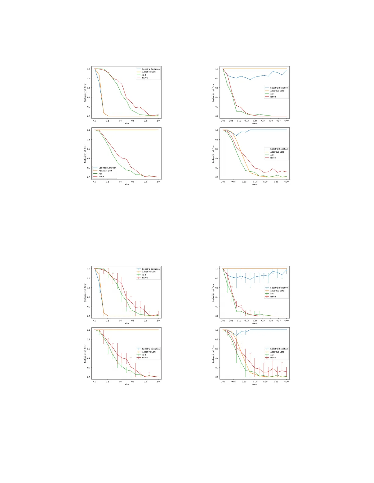
Activ e Seriation: Efﬁcient Ordering Recov ery with Statistical Guarantees James Cheshir e Y ann Issartel L TCI, Télécom Paris, Institut Polytechnique de P aris Abstract Activ e seriation aims at recov ering an unknown ordering of n items by adaptiv ely querying pairwise similarities. The observations are noisy measurements of entries of an underlying n × n permuted Robinson matrix, whose permutation encodes the latent ordering. The framew ork allows the algorithm to start with partial information on the latent ordering, including seriation from scratch as a special case. W e propose an active seriation algorithm that provably recov ers the latent ordering with high probability . Under a uniform separation condition on the similarity matrix, optimal performance guarantees are established, both in terms of the probability of error and the number of observ ations required for successful recov ery . 1 Introduction The seriation problem in v olves ordering n items based on noisy measurements of pairwise similarities. This reordering problem originates in archaeology , where it was used for the chronological dating of grav es [Robinson, 1951]. More recently , it has found applications in data science across various domains, including en velope reduction for sparse matrices [Barnard et al., 1995], read alignment in de nov o sequencing [Garriga et al., 2011, Recanati et al., 2017], time synchronization in distrib uted networks [Elson et al., 2004, Giridhar and Kumar, 2006], and interval graph identiﬁcation [Fulkerson and Gross, 1965]. In many of these settings, pairwise measurements can be made in an adaptiv e fashion, lev eraging information from previously chosen pairs. Moti v ated by these applications, we study the problem of recov ering an accurate item ordering from a sequence of activ ely selected pairwise measurements. The classical seriation problem has attracted substantial attention in the theoretical literature [Atkins et al., 1998, F ogel et al., 2013, Janssen and Smith, 2022, Giraud et al., 2023, Cai and Ma, 2023, Issartel et al., 2024]. In this line of w ork, the learner recei ves a single batch of observ ations, whereas in the activ e setting considered in this paper , the algorithm can adaptiv ely select which pairs to observe; to the best of our knowledge, this acti v e seriation setting has not been previously analyzed. Related problems include adaptive ranking and sorting under noisy observ ations [Jamieson and Now ak, 2011, Brav erman and Mossel, 2009, Heckel et al., 2019]. Howe ver , these problems typically rely on pairwise comparisons (e.g., is item i preferred to item j ?) to infer a total order . In contrast, seriation builds on pairwise similarity scores that encode proximity in the underlying ordering. This distinction leads to different statistical and algorithmic challenges. Problem setup. In the seriation paradigm, we assume the existence of an unkno wn symmetric matrix M representing pairwise similarities between a collection of n items. The matrix M is structured so that the similarities M ij are correlated with an unknown underlying ordering of the items, which is encoded by a permutation π = ( π 1 , . . . , π n ) of [ n ] . The similarity M ij between items i and j tends to be large when their positions π i and π j are close, and small when they are f ar 39th Conference on Neural Information Processing Systems (NeurIPS 2025). apart. T o model this structure formally , the literature assumes that M is a Robinson matrix whose ro ws and columns have been permuted by the latent permutation π [Fogel et al., 2013, Recanati et al., 2018, Janssen and Smith, 2022, Giraud et al., 2023]; see Section 2.1 for a formal presentation. W e consider a general framew ork in which the algorithm may be initialized with partial information on the latent ordering π . Speciﬁcally , it can be provided with a correct ordering of a subset of the items that is consistent with π . This setting includes seriation from scratch as the special case where no such information is giv en initially . The algorithm adaptiv ely selects pairs of items and observes noisy measurements of their similarities. A total of T such observations are collected, and the noise is controlled by an unkno wn parameter σ . The goal is to recov er the latent ordering π of the n items from these T observ ations. W e ev aluate the performance of an estimator ˆ π by its probability of failing to identify π . See Section 2 for details. Contribution. W e introduce Active Seriation by Iterative Insertion (ASII), an acti ve procedure for estimating the ordering π . Unlike most existing seriation methods, which are non-active, ASII is remarkably simple, runs in polynomial time, and yet achieves optimality guarantees both in terms of error probability and sample complexity . In the general framew ork considered in this paper, we analyze the performance of ASII and es- tablish exponential upper bounds on its probability of error . In the special case of seriation from scratch, where no prior ordering information is av ailable, we provide a sharp characterization of the statistical difﬁculty of ordering recovery o ver the class of similarity matrices with minimal gap ∆ between adjacent coefﬁcients. This difﬁculty is gov erned by the signal-to-noise ratio (SNR) of order ∆ 2 T / ( σ 2 n ) , which can be interpreted as the number of observations per item, T /n , multiplied by the SNR per observation, (∆ /σ ) 2 . Our results identify a phase transition at the critical lev el SNR ≍ ln n : below this threshold, ordering reco very is information-theoretically impossible, while above it, ASII achiev es recov ery with a probability of error that decays exponentially fast with the SNR. Moreover , we show that no algorithm can achie v e a faster decay rate, establishing optimality in this regime. Finally , we illustrate the performance of ASII through numerical experiments and a real-data applica- tion. 1.1 Related work Classical seriation. The non-active seriation problem was ﬁrst addressed by [Atkins et al., 1998] in the noiseless setting, using a spectral algorithm. Subsequent works analyzed this approach under noise [Fogel et al., 2013, Giraud et al., 2023, Natik and Smith, 2021], typically relying on strong spectral assumptions to establish statistical guarantees. More recent contributions proposed alternativ e polynomial-time algorithms with guarantees under diff erent and sometimes weaker assumptions [Janssen and Smith, 2022, Giraud et al., 2023, Cai and Ma, 2023, Issartel et al., 2024]. Our analysis falls within the line of work on Lipschitz-type assumptions [Giraud et al., 2023, Issartel et al., 2024], as our ∆ -separation condition can be viewed as a lo wer Lipschitz requirement. Statistical-computational gaps. Prior studies ha ve suggested statistical–computational gaps in the non-activ e seriation problem [Giraud et al., 2023, Cai and Ma, 2023, Berenfeld et al., 2024], where known polynomial-time algorithms fall short of achie ving statistically optimal rates under certain noise regimes or structural assumptions. While some of these g aps hav e recently been closed [Issartel et al., 2024], the resulting algorithms tend to be complex and may not scale well in practice. In contrast, in the activ e setting, we show that a simple and computationally ef ﬁcient algorithm achiev es statistically optimal performance. Bandit models. In classical multi-armed bandits (MAB) [Bubeck and Cesa-Bianchi, 2012], each arm yields independent rew ards, and the goal is to maximize cumulati ve re ward or identify the best arm. In contrast, in activ e seriation, each query ( i, j ) measures the similarity between two interdependent items, and all measurements must be consistent with a single latent ordering. This interdependence prev ents a direct application of standard MAB algorithms such as UCB or Thompson Sampling, which treat arms as independent and do not exploit structural relationships between them. Algorithmically , our approach is related to noisy binary search and thresholding bandits [Feige et al., 1994, Karp and Kleinberg, 2007, Ben-Or and Hassidim, 2008, Nowak, 2009, Emamjomeh- Zadeh et al., 2016, Cheshire et al., 2020, Cheshire et al., 2021], which rely on adaptive querying 2 under uncertainty . Howe ver , these methods operate on low-dimensional parametric models, whereas seriation in v olves a combinatorial ordering that must remain globally consistent across item pairs. Active ranking. A related b ut distinct problem is acti ve ranking [Heckel et al., 2019, Shah and W ainwright, 2017], where a learner infers a total order based on noisy pairwise comparisons or latent score estimates. Extensions include Borda, expert, and bipartite ranking [Saad et al., 2023, Cheshire et al., 2023]. These methods typically assume that each item is associated with an intrinsic scalar score, and that pairwise feedback e xpresses a directional preference between items. In contrast, seriation relies on pairwise similarity information, which encodes proximity rather than preference. Recov ering the latent ordering therefore requires global consistency among all pairwise similarities, making the problem more constrained and structurally different from standard ranking tasks. 2 Active Seriation: Problem Setup 2.1 Similarity matrix and ordering Gi ven a collection of items [ n ] := { 1 , . . . , n } , let M = [ M ij ] 1 ≤ i,j ≤ n denote the (unknown) similarity matrix , where the coefﬁcient M ij ∈ R measures the similarity between items i and j . Our structural assumption on M is related to the class of Robinson matrices, introduced belo w . Deﬁnition 2.1. A matrix R ∈ R n × n is called a Robinson matrix (or R-matrix) if it is symmetric and R i,j > R i − 1 ,j and R i,j > R i,j +1 , for all i ≤ j on the upper triangle of R . The entries of a Robinson matrix decrease as one mov es aw ay from the (main) diagonal (see Figure 1, left). In other words, each row / column is unimodal and attains its maximum on the diagonal. Figure 1: R-matrix & a permuted v ersion. Follo wing [Atkins et al., 1998], a matrix is said to be pr e-R if it can be transformed into an R-matrix by simul- taneously permuting its rows and columns (Figure 1, right). In this paper, we assume the similarity matrix M is pre-R, i.e., M = R π := [ R π i ,π j ] 1 ≤ i,j ≤ n , (1) for some R-matrix R and some permutation π = ( π 1 , . . . , π n ) of [ n ] . The permutation π represents the latent or dering of the items. In (1) , the similarities M ij reﬂect the ordering π as follows: M ij tends to be larger when the positions π i and π j are close together , and smaller when they are far apart. Remark 1. The items have exactly two orderings: if π is an ordering, then the r e verse permuta- tion π rev , deﬁned by π rev i = n + 1 − π i , is also an ordering . Indeed, if M = R π , then M = R rev π rev , wher e R rev is obtained by r e versing the r ows and columns of R . In the sequel, we refer to either of these two or derings as the latent or dering. 2.2 Active observation model In the activ e seriation problem, the algorithm sequentially queries T pairs of items and receiv es noisy observations of their pairwise similarities, encoded by the unknown similarity matrix M in (1) . The goal is to recov er the latent ordering π of the n items from these noisy observ ations. Initially , the algorithm is provided with partial information on the latent ordering π : it receiv es as input a correct ordering ˜ π of the items { 1 , . . . , n − ˜ n } , corresponding to the restriction of π to this subset. This frame work interpolates between online seriation ( ˜ n = 1 ), where a single item is inserted into an existing ordering, and seriation from scratch ( ˜ n = n ). More precisely , for some ˜ n ∈ [ n ] , the algorithm is gi ven a permutation ˜ π = ( ˜ π 1 , . . . , ˜ π n − ˜ n ) of [ n − ˜ n ] satisfying 1 ∀ i, j ∈ [ n − ˜ n ] , π i < π j ⇐ ⇒ ˜ π i < ˜ π j . (2) 1 In full generality , condition (2) should be assumed to hold either for the latent ordering π or for its re verse π rev ; for simplicity of exposition, we state it in terms of π , as this distinction plays no essential role in what follows. 3 In other words, the input permutation ˜ π preserves the relati v e order of the items { 1 , . . . , n − ˜ n } in the latent ordering π . At each round t = 1 , . . . , T , the algorithm selects a pair ( i t , j t ) with i t  = j t , possibly depending on the outcomes of pre vious queries. It then recei ves a noisy observ ation of the similarity M i t j t , gi ven by a σ -sub-Gaussian random variable 2 with mean M i t j t . This sub-Gaussian setting cov ers standard observation models, including Gaussian noise and bounded random v ariables. After T queries, the algorithm outputs a permutation ˆ π of [ n ] as its estimate of the latent ordering π . 2.3 Error probability and minimal gap The algorithm is considered successful if ˆ π recov ers either π or its rev erse π rev , as both permutations are valid orderings (Remark 1). The probability of error is thus deﬁned as: 3 p M ,T := P M ,T { ˆ π  = π and ˆ π  = π rev } , (3) where the probability is ov er the randomness in the T observations collected on the matrix M . A ke y quantity in our analysis of (3) is the separation between consecuti ve entries in the underlying R-matrix. Speciﬁcally , for any pre-R matrix M as in (1), we deﬁne its minimal gap as ∆ M := min 1 0 (by Deﬁnition 2.1) and that ∆ M is well-deﬁned ev en though M can be associated with dif ferent R-matrices (Remark 1). Some of our guarantees are stated o ver classes of matrices with a prescribed minimal gap. Namely , for any ∆ > 0 , we introduce M ∆ :=  M ∈ R n × n : M is pre-R, and ∆ M ≥ ∆  , (5) as the set of pre-R matrices with minimal gap at least ∆ . T o simplify the presentation of our ﬁndings, we focus on the challenging regime where ∆ σ ≤ 1 , ( σ > 0) , (6) i.e., the signal-to-noise ratio per observ ation is at most 1 . This e xcludes mildly stochastic regimes where the problem has essentially the same difﬁculty as in the noiseless case. 3 Seriation procedur e A S I I (Active Seriation by Iterative Insertion) reconstructs the underlying ordering by iterati vely inserting each ne w item into an already ordered list. At iteration k , gi ven a current estimated ordering ˆ π ( k − 1) of the items { 1 , . . . , k − 1 } , the algorithm inserts item k at its correct position to form an updated ordering ˆ π ( k ) of { 1 , . . . , k } . This process is repeated until the full ordering of all n items is obtained. The algorithm is fully data-driv en: it takes as input only the sampling budget T ; it does not rely on any kno wledge of the noise parameter σ , the similarity matrix M , nor its minimal gap ∆ M . T o perform this insertion efﬁciently , two ke y subroutines are used: (i) Local comparison rule. T o decide where to insert k , the algorithm must compare its position relati ve to items already ordered in ˆ π ( k − 1) . This is achie ved through the subroutine T E S T , which determines whether k lies to the left, in the middle, or to the right of two reference items ( l, r ) . (ii) Efﬁcient insertion strategy . T o minimize the number of comparisons, the algorithm performs a binary search ov er the current ordering, where each comparison is made via T E S T . Because these tests are noisy , the procedure is further stabilized through a backtracking mechanism. 2 A random variable X is said to be σ -sub-Gaussian if E [exp( uX )] ≤ exp  u 2 σ 2 2  for all u ∈ R . 3 This lack of identiﬁability between π and π rev persists in the seriation from scratch case, since condition (2) is vacuous. 4 (i) Local comparison rule. Gi ven two items ( l, r ) such that π l < π r , the goal is to determine whether k lies to the left, in the middle, or to the right of ( l, r ) in the unknown ordering π . Formally , this means deciding whether π k < π l , or π k ∈ ( π l , π r ) , or π k > π r , respectiv ely . The subroutine T E S T is based on the follo wing property of Robinson matrices: when k lies between l and r , its similarity to both l and r tends to be higher than the similarity between l and r themselves. Accordingly , T E S T compares the three empirical similarities c M kl , c M kr , and c M lr , and identiﬁes the smallest one as the pair of items that are farthest apart. F or example, if c M lr is the smallest, then k lies in the middle. The pseudocode of T E S T is provided in Appendix B. Each call to the subroutine T E S T is performed with a limited sampling budget, typically of order O ( T / ( ˜ n log 2 k )) , in order to be sampling-efﬁcient. With such a b udget, individual tests are not designed to be reliable with high probability . This design trades local test accuracy for global budget efﬁcienc y; occasional incorrect tests are later corrected by a backtracking mechanism. Remark: Higher reliability is required only at a fe w critical steps of A S I I (e.g., during the initialization of the binary search), where a larger b udget of order O ( T / ˜ n ) is allocated to ensure correctness with high probability . (ii) Efﬁcient insertion strategy . The idea of incorporating backtracking into a noisy search has appeared in se veral studies, e.g., [Feige et al., 1994, Ben-Or and Hassidim, 2008, Emamjomeh-Zadeh et al., 2016, Cheshire et al., 2021]. Here, we adopt this general principle to design a robust insertion mechanism that remains reliable under noisy relational feedback. At this stage of the algorithm, the items { 1 , . . . , k − 1 } hav e already been placed into an estimated ordering ˆ π ( k − 1) = ( ˆ π ( k − 1) 1 , . . . , ˆ π ( k − 1) k − 1 ) constructed so far . T o insert the ne w item k into this list, we use the subroutine B I N A RY & B A C K T R A C K I N G S E A R C H ( B B S), which determines the relative position of k within the current ordering ˆ π ( k − 1) . The search proceeds by repeatedly using the subroutine T E S T to decide whether k lies in the left or right half of a candidate interval, thereby narrowing do wn the possible insertion range. Because the outcomes of T E S T are noisy , e v en a single incorrect decision can misguide the search and lead to an erroneous ﬁnal placement. A naiv e ﬁx would be to allocate man y samples per T E S T to ensure highly reliable outcomes, b ut this would increase the sample complexity and undermine the beneﬁt of activ e sampling. Instead, B B S uses a small number of samples per T E S T , of order O ( T / ( ˜ n log 2 k )) , just enough to ensure a constant success probability (e.g., around 3 / 4 ). Backtracking then acts as a correctiv e mechanism that pre vents local errors from propagating irre versibly . The backtracking mechanism operates as follo ws: the algorithm k eeps track of pre viously explored intervals and performs sanity checks at each step to detect inconsistencies in the search path. When an inconsistency is detected, it backtracks to an earlier interval and resumes the search. This pre vents local mistakes from propagating irre versibly . Theoretical analysis shows that, as long as the number of correct local decisions outweighs the number of incorrect ones — an e v ent that occurs with high probability under the assumption M ∈ M ∆ — the ﬁnal insertion position is accurate. Hence, the backtracking mechanism allo ws the algorithm to detect and correct occasional local errors. As a result, we can use only a small number of samples per call to T E S T , while still ensuring correct insertions at the global level. The A S I I procedure thus provides both sampling ef ﬁciency and robustness, despite noisy observ ations. A pseudocode of this procedure is given in Appendix B. 4 Perf ormance analysis W e study the fundamental limits of ordering recovery in activ e seriation, deriving information- theoretic lower bounds and algorithmic upper bounds on the error probability deﬁned in (3). 4.1 Upper bounds for ASII W e analyze the performance of A S I I when the algorithm is provided with a permutation ˜ π of the items { 1 , . . . , n − ˜ n } , consistent with the latent ordering π of the n items. The follo wing theorem giv es an upper bound on the error probability of ASII for recov ering π . Its proof is in Appendix C. 5 Theorem 4.1 (Upper bound with partial information) . Ther e exists an absolute constant c 0 > 0 such that the following holds. Let n ≥ 3 and ˜ n ∈ [ n ] , and assume that the input permutation ˜ π of [ n − ˜ n ] satisﬁes (2) . Let (∆ , σ, T ) be suc h that condition (6) holds and ∆ 2 T σ 2 ˜ n ≥ c 0 ln n . If M ∈ M ∆ , then the err or pr obability of A S I I satisﬁes p M ,T ≤ exp  − 1 2400 ∆ 2 T σ 2 ˜ n  . (7) Once the SNR, ∆ 2 T / ( σ 2 ˜ n ) , exceeds a logarithmic threshold in n , the error probability of A S I I decays exponentially fast with the SNR. W e emphasize that ASII achiev es this performance without requiring any kno wledge of the model parameters (∆ , σ ) . Beyond this uniform guarantee ov er the class M ∆ , the performance of ASII admits a ﬁner, instance- dependent characterization. The same bound holds with ∆ replaced by the true minimal gap ∆ M of the underlying matrix M (deﬁned in (4) ). Precisely , for the instance-dependent SNR M = ∆ 2 M T / ( σ 2 ˜ n ) , the bound becomes p M ,T ≤ exp( − SNR M / 2400) whenever SNR M ≥ c 0 ln n . 4.2 Minimax optimal rates for seriation from scratch W e establish matching information-theoretic lower bounds in the case of acti ve seriation from scratch ( ˜ n = n ), where no prior ordering information is available. This analysis identiﬁes two regimes, depending on whether the SNR is below or abo ve a critical threshold. 4.2.1 Impossibility r egime. When the SNR satisﬁes ∆ 2 T σ 2 n ≲ ln n , no algorithm can recover the ordering with v anishing error probability . The follo wing theorem formalizes this impossibility , establishing a constant lower bound on the error probability (3) for an y algorithm in this regime. Theorem 4.2 (Impossibility regime) . Ther e exists an absolute constant c 1 > 0 such that the following holds. Let n ≥ 9 and (∆ , σ, T ) be suc h that ∆ 2 T σ 2 n ≤ c 1 ln n . Then, for any algorithm A , ther e e xists a matrix M ∈ M ∆ such that the err or pr obability of A satisﬁes p M ,T ≥ 1 / 2 . As expected, the impossibility regime is more pronounced when the minimal gap ∆ is small or when the noise parameter σ is large. T o escape this regime, the number of observations per item, T /n , must grow at least quadratically with σ/ ∆ (up to logarithmic f actors). The proof is in Appendix E. 4.2.2 Recovery r egime. In the complementary regime where the SNR satisﬁes ∆ 2 T σ 2 n ≳ ln n , exact recov ery becomes achie vable. The A S I I algorithm attains an exponentially small error probability , and this rate is minimax optimal ov er the class M ∆ , up to absolute constants in the exponent. Speciﬁcally , the upper bound in this regime follows directly from Theorem 4.1 by taking ˜ n = n . If ∆ 2 T σ 2 n ≥ c 0 ln n , (8) where c 0 is the same absolute constant as in Theorem 4.1, then for any M ∈ M ∆ , the probability of error of A S I I satisﬁes, p M ,T ≤ exp  − 1 2400 ∆ 2 T σ 2 n  . Con versely , the next theorem giv es a matching lower bound, showing that no algorithm can achiev e a faster error decay than exponential in the SNR. Its proof is in Appendix E. Theorem 4.3 (Reco very re gime) . Let n ≥ 4 and (∆ , σ, T ) be such that condition (8) holds. Then, for any algorithm A , ther e exists M ∈ M ∆ such that the err or probability of A satisﬁes p M ,T ≥ exp  − 8 ∆ 2 T σ 2 n  . 6 T ogether , Theorems 4.2 and 4.3 delineate the statistical landscape of acti ve seriation from scratch, establishing a sharp phase transition between impossibility and recovery at the critical SNR level ∆ 2 T σ 2 n ≍ ln n . 4.2.3 Discussion: intrinsic hardness and in variance to model assumptions. Both lo wer bounds (Theorems 4.2 and 4.3) are established under a Gaussian noise model with centered, homoscedastic entries of variance σ 2 , whereas our upper bound is proved in the more general sub-Gaussian setting allowing heterogeneous noise le vels. Since these bounds match, potential heterogeneity in the noise variances does not af fect the minimax rates (at least in terms of e xponential decay in SNR). Moreov er , the lo wer bounds are deriv ed for the simple, afﬁne, T oeplitz matrix R ij = ( n − | i − j | )∆ , (9) yet the attainable rates coincide with those obtained under the general assumption M ∈ M ∆ . Hence, allowing heterogeneous, non-T oeplitz matrices comes at no statistical cost. This may appear surprising, since the T oeplitz assumption is classical in batch seriation (e.g., [Cai and Ma, 2023]). Even when the latent matrix is fully known, as in the one-parameter family (9) with kno wn param- eter ∆ , the attainable rates remain unchanged. This indicates that the hardness of active seriation arises from the combinatorial nature of the latent ordering, rather than from uncertainty about the latent matrix. 4.3 Sample complexity for high probability r ecov ery W e summarize our results in terms of sample complexity , deﬁned as the number of observations required to achie ve e xact recov ery with probability at least 1 − 1 /n 2 . Combining the impossibility result of Theorem 4.2 with the recovery guarantee of Theorem 4.1, we obtain a sharp characterization of the sample complexity in the from-scratch case ( ˜ n = n ). Corollary 4.4 (Sample comple xity) . Let n ≥ 9 and ˜ n ∈ [ n ] , and assume that the input permutation ˜ π of [ n − ˜ n ] satisﬁes (2) . Let (∆ , σ ) be such that condition (6) holds. Then A S I I ac hieves exact r ecovery with pr obability at least 1 − 1 /n 2 , if T ≳ σ 2 ˜ n ln n ∆ 2 . In particular , in the fr om-scratch case ˜ n = n , the minimax-optimal number of observations r equir ed for exact r eco very with pr obability at least 1 − 1 /n 2 , satisﬁes T ⋆ ≍ σ 2 n ln n ∆ 2 . Thus, in activ e seriation from scratch, A S I I attains the minimax-optimal sample complexity T ⋆ , which depends transparently on the problem parameters (∆ , σ, n ) . Crucially , A S I I can achiev e high probability recov ery with a number of queries T ≪ n 2 , highlighting a substantial advantage ov er the classical batch setting where all n 2 pairwise similarities are observed. 4.4 Extension beyond unif orm separation Our analysis so far has focused on exact recovery under the uniform separation assumption M ∈ M ∆ . While this assumption is natural for characterizing the fundamental limits of exact recovery , it is also idealized: in practice, some items may be nearly indistinguishable in terms of their pairwise similarities, making their relativ e ordering statistically impossible to recov er . W e therefore consider arbitrary pre-R matrices M , as deﬁned in model (1) , without any separation assumption. Even in this setting, a direct e xtension of the A S I I procedure continues to provide meaningful and statistically optimal guarantees: it correctly recovers the relati ve ordering of items that are sufﬁciently well separated. Algorithmic extension of ASII. The procedure follo ws the same iterativ e insertion scheme as our A S I I algorithm, but takes as input a tolerance parameter ˜ ∆ > 0 , which sets the resolution at which the algorithm attempts to distinguish items. Now , when A S I I identiﬁes a candidate insertion location for a new item in the current ordering, this location is checked through an additional high-probability validation test at precision ˜ ∆ / 2 . The item is inserted if the test succeeds; otherwise it is discarded and does not appear in the ﬁnal output. 7 As a consequence, this extension no longer outputs a permutation ˆ π of all n items. Instead, it returns a subset S ⊂ [ n ] together with a rank map ˆ π : S → { 1 , . . . , | S |} , which serves as an estimator of the relativ e ordering of the items in S . The corresponding pseudo-code is deferred to Appendix D. Robustness bey ond unif orm separation. W e no w state rob ustness guarantees for the e xtension described above. T o this end, we introduce a notion of ∆ -maximality , inspired by the class M ∆ deﬁned in (5) . Speciﬁcally , for any subset S ⊂ [ n ] , we write M S for the submatrix of the similarity matrix M restricted to the items in S . By a slight ab use of notation, we write M S ∈ M ∆ to mean that M S is pre-R and satisﬁes ∆ M S ≥ ∆ , where ∆ M S is the minimal gap deﬁned in (4). Deﬁnition 4.5 ( ∆ -maximal subset) . F or any ∆ > 0 , a subset S ⊂ [ n ] is said to be ∆ -maximal if M S ∈ M ∆ and M S ∪{ k } / ∈ M ∆ for all k ∈ [ n ] \ S . Intuitiv ely , a ∆ -maximal subset cannot be enlarged without adding items that are too similar (within ∆ ) to those already in S . W e now sho w that the guarantee of Theorem 4.1 can be extended be yond the uniformly separated setting, to any pre-R matrix M , by operating at a user-chosen resolution le vel ˜ ∆ . The conditions on the parameters are the same as in Theorem 4.1, with ∆ replaced by the input parameter ˜ ∆ ; that is: ˜ ∆ σ ≤ 1 , ˜ ∆ 2 T σ 2 ˜ n ≥ c ln n . (10) Theorem 4.6 (Guarantees beyond uniform separation) . Ther e e xist absolute constants c, c ′ > 0 such that the following holds. Let n ≥ 3 , ˜ n ∈ [ n ] and the input permutation ˜ π of [ n − ˜ n ] satisfy (2) . Let ( ˜ ∆ , σ, T ) be such that (10) holds. Then, for any pr e-R matrix M ∈ R n × n , the algorithmic extension of A S I I outputs, with pr obability at least 1 − exp  − c ′ ˜ ∆ 2 T σ 2 ˜ n  , a ˜ ∆ -maximal subset S ⊂ [ n ] in the sense of Deﬁnition 4.5, and a corr ect or dering ˆ π S of the items in S . The proof is giv en in Appendix D. 5 Empirical results W e illustrate the behavior of A S I I through numerical experiments and a real-data example. Numerical simulations. W e assess the empirical beha vior of A S I I on synthetic data and compare it to three benchmark methods: (i) the batch seriation algorithm A DA P T I V E S A M P L I N G [Cai and Ma, 2023], (ii) the batch S P E C T R A L S E R I A T I O N [Atkins et al., 1998], and (iii) an activ e, naiv e insertion variant of A S I I without backtracking. Since, to the best of our knowledge, the literature does not contain seriation methods designed for the acti v e setting, these three procedures serve as reference points. All methods are e v aluated under identical sampling budgets on four representati ve scenarios, cov ering both homogeneous (T oeplitz) and non-homogeneous (non-T oeplitz), Robinson matrices. Full experimental details are deferred to Appendix G. Figure 2 provides a visual illustration of the four scenarios considered. Scenario (1) corresponds to a T oeplitz Robinson structure, while the remaining scenarios (2-3-4) depart from the T oeplitz assumption and exhibit more heterogeneous Robinson geometries. Figure 2: Robinson matrices for scenarios (1)-(4), from left to right. Figure 3 reports the empirical probability of error of all methods as a function of the minimal gap ∆ . Across all four scenarios, A S I I consistently outperforms the naive iterati ve insertion procedure, highlighting the beneﬁts of its backtracking corrections; these gains are consistent with the log arithmic improv ement predicted by our theoretical analysis. 8 As expected, in scenario (1), where the underlying matrix is T oeplitz, A S I I performs below the two batch methods, which are kno wn to perform well in this setting. This beha vior can be attributed to the fact that A S I I is designed for general Robinson matrices and does not exploit T oeplitz regularity (unlike its competitors); moreo ver , its sampling budget is distributed across multiple binary-search iterations, which can be less ef ﬁcient than batch sampling. This does not contradict our theoretical guarantees, which establish rates up to absolute constants that are not characterized by the analysis and may be large for acti ve, iterati v e procedures such as A S I I . In contrast, in the heterogeneous (non-T oeplitz) scenarios (2-3-4), A S I I remains consistently accurate, whereas both batch methods exhibit unstable beha vior and may fail entirely in some cases. Overall, these experiments illustrate that A S I I maintains stable empirical performance across various scenarios, and can be particularly ef fecti ve on matrices with localized variations (scenarios 2-3-4), where batch methods tend to struggle. Figure 3: Empirical error probabilities for A S I I and three benchmark methods as the parameter ∆ varies. Scenarios (1-2-3-4) are displayed from left to right and top to bottom. Each e xperiment uses n = 10 items and T = 10 , 000 observations. For each value of ∆ , 100 Monte Carlo runs are split into 10 equal groups; error bars show the 0 . 1 and 0 . 9 quantiles of the empirical error across groups. Application to real data. W e further assess the robustness of A S I I on real single-cell RNA sequencing data (human primordial germ cells, from [Guo et al., 2015], previously analyzed by [Cai and Ma, 2023]). Although such biological data depart substantially from the idealized Robinson models assumed in our theory , A S I I still produces a meaningful reordering of the empirical similarity matrix, revealing coherent de velopmental trajectories among cells. This example highlights the potential practical relev ance of the proposed approach beyond the stylized assumptions of our theoretical framew ork. Full e xperimental details are provided in Appendix G. Figure 4: Similarity matrix M of a single-cell RNA-seq dataset before and after reordering by ASII. The recov ered ordering rev eals a clear block-diagonal structure consistent with dev elopmental progression: dissimilar re gions (blue) are pushed to the boundaries, while groups of highly similar cells (yellow and green) align along the diagonal. 9 6 Discussion This work introduces an active-learning formulation of the seriation problem, together with sharp theoretical guarantees and a simple polynomial-time algorithm. W e characterize a phase transition in sample complexity gov erned by the SNR = ∆ 2 T / ( σ 2 n ) : recov ery is impossible when SNR ≲ ln n , while A S I I achiev es near optimal performances once this threshold is e xceeded. Our analysis highlights how adapti v e sampling combined with corrective backtracking can substantially impro ve statistical efﬁcienc y . W e now turn to a discussion of se veral complementary aspects of the problem. Noise regimes. Our analysis focused on the stochastic regime where the per-observ ation signal-to- noise ratio ∆ /σ is at most 1 , which captures the most challenging setting for active seriation. The results, ho wev er , extend naturally to less noisy regimes ( ∆ /σ > 1 ): in that case, accurate recovery requires only T ≳ n ln n queries, reﬂecting the intrinsic O ( n ln n ) cost of performing n adaptiv e binary insertions. Further details are pro vided in Appendix A.1. Gain from active learning. Our activ e framew ork enables recovery of the underlying ordering without observing the entire similarity matrix. Whereas batch approaches require O ( n 2 ) observa tions, our active algorithm A S I I succeeds with only T ≳ ( σ/ ∆) 2 n ln n samples. This corresponds to a fraction ln n (∆ /σ ) 2 n of the full matrix and yields a substantial reduction in sample comple xity , as long as ∆ /σ is not too small. This gain arises from the ability of adaptiv e sampling to draw information from a well-chosen, small subset of pairwise similarities, from which the entire matrix can be reordered, achieving strong statistical guarantees under limited sampling b udgets. In certain scenarios, when dif ferences between candidate orderings are highly localized, our activ e algorithm can succeed under weaker signal conditions than some batch methods, see Appendix A.2 for a detailed comparativ e example. Fixed-budget f ormulations. Throughout this work, we focused on the ﬁxed-b udget setting, where the total number of samples T is ﬁxed in advance and the objecti ve is to minimize the error probability within this budget. This way , the algorithm does not require prior knowledge of the noise parameter σ , nor of the minimal signal gap ∆ M of the latent matrix M ; it simply allocates the av ailable b udget T across tests. Y et, its performance depends on the unknown σ and ∆ M through the signal-to-noise ratio SNR M = ∆ 2 M T / ( σ 2 n ) , which determines the achiev able accurac y . Potential applications. Seriation techniques are broadly relev ant in domains where pairwise simi- larity information reﬂects a latent one-dimensional structure. Examples include genomic sequence alignment, where seriation helps reorder genetic fragments by similarity , and recommendation sys- tems, where item-item similarity matrices can rev eal latent preference orderings. W e also illustrated, on real single-cell RN A sequencing data, that A S I I can recover biologically meaningful trajectories despite the data departing strongly from our theoretical model. These settings often inv olve noisy or costly pairwise measurements, for which acti ve seriation pro vides an appealing alternati ve to batch reordering methods. Future directions. W e also proposed an extension to settings where the uniform separation as- sumption does not hold, in which A S I I outputs an ordering of a subset of well-separated items. How to exploit more global ordering structure be yond this setting is an important open question. Another natural extension is to study the ﬁxed-conﬁdence setting, where the algorithm must adaptively decide when to stop sampling in order to achie ve a prescribed conﬁdence le vel. Such a formulation would typically require v ariance-a ware sampling policies and data-driven stopping rules, possibly in v olving online estimation of σ . De veloping such an adapti ve, ﬁx ed-conﬁdence version of A S I I is an interesting av enue for future work. Acknowledgements The work of J. Cheshire is supported by the FMJH, ANR-22-EXES-0013. 10 References [Atkins et al., 1998] Atkins, J. E., Boman, E. G., and Hendrickson, B. (1998). A spectral algorithm for seriation and the consecutiv e ones problem. SIAM Journal on Computing, 28(1):297–310. [Barnard et al., 1995] Barnard, S. T ., Pothen, A., and Simon, H. (1995). A spectral algorithm for en velope reduction of sparse matrices. Numerical linear algebra with applications , 2(4):317–334. [Ben-Or , 1983] Ben-Or , M. (1983). Lo wer bounds for algebraic computation trees. In Proceedings of the Fifteenth Annual A CM Symposium on Theory of Computing, STOC ’83. [Ben-Or and Hassidim, 2008] Ben-Or , M. and Hassidim, A. (2008). The bayesian learner is optimal for noisy binary search (and pretty good for quantum as well). In 2008 49th Annual IEEE Symposium on Foundations of Computer Science, pages 221–230. IEEE. [Berenfeld et al., 2024] Berenfeld, C., Carpentier , A., and V erzelen, N. (2024). Seriation of t {\ oe } plitz and latent position matrices: optimal rates and computational trade-offs. arXiv preprint [Brav erman and Mossel, 2009] Brav erman, M. and Mossel, E. (2009). Sorting from noisy informa- tion. arXi v preprint arXi v:0910.1191. [Bubeck and Cesa-Bianchi, 2012] Bubeck, S. and Cesa-Bianchi, N. (2012). Re gret analysis of stochastic and nonstochastic multi-armedbandit problems. [Cai and Ma, 2023] Cai, T . T . and Ma, R. (2023). Matrix reordering for noisy disordered matrices: Optimality and computationally efﬁcient algorithms. IEEE transactions on information theory , 70(1):509–531. [Cheshire and Clémençon, 2025] Cheshire, J. and Clémençon, S. (2025). Active bipartite ranking with smooth posterior distrib utions. In The 28th International Conference on Artiﬁcial Intelligence and Statistics. [Cheshire et al., 2023] Cheshire, J., Laurent, V ., and Clémençon, S. (2023). Activ e bipartite ranking. In Thirty-sev enth Conference on Neural Information Processing Systems. [Cheshire et al., 2020] Cheshire, J., Ménard, P ., and Carpentier , A. (2020). The inﬂuence of shape constraints on the thresholding bandit problem. In Conference on Learning Theory , pages 1228– 1275. PMLR. [Cheshire et al., 2021] Cheshire, J., Ménard, P ., and Carpentier , A. (2021). Problem dependent view on structured thresholding bandit problems. In International Conference on Machine Learning , pages 1846–1854. PMLR. [Cormen et al., 2009] Cormen, T . H., Leiserson, C. E., Rivest, R. L., and Stein, C. (2009). Introduction to Algorithms, Third Edition. The MIT Press, 3rd edition. [Elson et al., 2004] Elson, J., Karp, R. M., P apadimitriou, C. H., and Shenker , S. (2004). Global synchronization in sensornets. In Farach-Colton, M., editor , LA TIN 2004: Theoretical Informatics , pages 609–624, Berlin, Heidelberg. Springer Berlin Heidelber g. [Emamjomeh-Zadeh et al., 2016] Emamjomeh-Zadeh, E., K empe, D., and Singhal, V . (2016). De- terministic and probabilistic binary search in graphs. In Proceedings of the forty-eighth annual A CM symposium on Theory of Computing, pages 519–532. A CM. [Falahatgar et al., 2017] Falahatgar , M., Orlitsky , A., Pichapati, V ., and Suresh, A. T . (2017). Max- imum selection and ranking under noisy comparisons. In Proceedings of the 34th International Conference on Machine Learning. [Feige et al., 1994] Feige, U., Raghav an, P ., Peleg, D., and Upfal, E. (1994). Computing with noisy information. SIAM Journal on Computing, 23(5):1001–1018. [Fogel et al., 2013] Fogel, F ., Jenatton, R., Bach, F ., and d’Aspremont, A. (2013). Conv ex relaxations for permutation problems. In Advances in Neural Information Processing Systems , pages 1016– 1024. [Fulkerson and Gross, 1965] Fulkerson, D. and Gross, O. (1965). Incidence matrices and interval graphs. P aciﬁc journal of mathematics, 15(3):835–855. [Garivier et al., 2019] Gari vier , A., Ménard, P ., and Stoltz, G. (2019). Explore ﬁrst, exploit ne xt: The true shape of regret in bandit problems. Mathematics of Operations Research, 44(2):377–399. 11 [Garriga et al., 2011] Garriga, G. C., Junttila, E., and Mannila, H. (2011). Banded structure in binary matrices. Kno wledge and information systems, 28(1):197–226. [Gerchinovitz et al., 2020] Gerchinovitz, S., Ménard, P ., and Stoltz, G. (2020). Fano’ s inequality for random variables. Statistical Science, 35(2):178–201. [Giraud et al., 2023] Giraud, C., Issartel, Y ., and V erzelen, N. (2023). Localization in 1d non- parametric latent space models from pairwise afﬁnities. Electronic Journal of Statistics , 17(1):1587–1662. [Giridhar and Kumar, 2006] Giridhar, A. and K umar, P . R. (2006). Distributed clock synchronization ov er wireless networks: Algorithms and analysis. In Proceedings of the 45th IEEE Conference on Decision and Control, pages 4915–4920. [Gu and Xu, 2023] Gu, Y . and Xu, Y . (2023). Optimal bounds for noisy sorting. In Proceedings of the 55th Annual A CM Symposium on Theory of Computing, pages 1502–1515. [Guo et al., 2015] Guo, F ., Y an, L., Guo, H., Li, L., Hu, B., Zhao, Y ., Y ong, J., Hu, Y ., W ang, X., W ei, Y ., et al. (2015). The transcriptome and dna methylome landscapes of human primordial germ cells. Cell, 161(6):1437–1452. [Hao et al., 2023] Hao, Y ., Stuart, T ., K o walski, M. H., Choudhary , S., Hoffman, P ., Hartman, A., Sriv asta va, A., Molla, G., Madad, S., Fernandez-Granda, C., and Satija, R. (2023). Dictionary learning for integrati ve, multimodal and scalable single-cell analysis. Nature Biotechnology. [Heckel et al., 2019] Heckel, R., Shah, N. B., Ramchandran, K., and W ainwright, M. J. (2019). Activ e ranking from pairwise comparisons and when parametric assumptions do not help. [Issartel et al., 2024] Issartel, Y ., Giraud, C., and V erzelen, N. (2024). Minimax optimal seriation in polynomial time. arXi v preprint arXi v:2405.08747. [Jamieson and Now ak, 2011] Jamieson, K. G. and No wak, R. (2011). Active ranking using pairwise comparisons. Adv ances in neural information processing systems, 24. [Janssen and Smith, 2022] Janssen, J. and Smith, A. (2022). Reconstruction of line-embeddings of graphons. Electronic Journal of Statistics, 16(1):331–407. [Karp and Kleinberg, 2007] Karp, R. M. and Kleinber g, R. (2007). Noisy binary search and its appli- cations. In Proceedings of the eighteenth annual A CM-SIAM symposium on Discrete algorithms , pages 881–890. Society for Industrial and Applied Mathematics. [Lattimore and Szepesvári, 2020] Lattimore, T . and Szepesvári, C. (2020). Bandit algorithms . Cam- bridge Univ ersity Press. [Natik and Smith, 2021] Natik, A. and Smith, A. (2021). Consistency of spectral seriation. arXiv preprint [Now ak, 2009] Now ak, R. (2009). The geometry of generalized binary search. arXic preprint [Recanati et al., 2017] Recanati, A., Brüls, T ., and d’Aspremont, A. (2017). A spectral algorithm for fast de nov o layout of uncorrected long nanopore reads. Bioinformatics, 33(20):3188–3194. [Recanati et al., 2018] Recanati, A., Kerdreux, T ., and d’Aspremont, A. (2018). Reconstructing latent orderings by spectral clustering. arXi v preprint arXi v:1807.07122. [Ren et al., 2019] Ren, W ., Liu, J. K., and Shrof f, N. (2019). On sample complexity upper and lo wer bounds for exact ranking from noisy comparisons. Advances in Neural Information Processing Systems, 32. [Robinson, 1951] Robinson, W . S. (1951). A method for chronologically ordering archaeological deposits. American Antiquity, 16(4):293–301. [Saad et al., 2023] Saad, E. M., V erzelen, N., and Carpentier , A. (2023). Acti ve ranking of experts based on their performances in man y tasks. In Proceedings of the 40th International Conference on Machine Learning. [Shah and W ainwright, 2017] Shah, N. B. and W ainwright, M. J. (2017). Simple, robust and optimal ranking from pairwise comparisons. The Journal of Machine Learning Research , 18(1):7246– 7283. [Soch et al., 2023] Soch et al., J. (2023). The book of statistical proofs. 12 A Additional discussion A.1 Beyond the stochastic regime ∆ /σ ≤ 1 T o simplify the presentation of our results, we have primarily focused on the challenging re gime where the signal-to-noise ratio per observation, ∆ /σ , is at most 1 . In this subsection, we discuss how our ﬁndings extend to less noisy re gimes where ∆ /σ may exceed 1 . In fact, our upper bound can be stated in a slightly more general form than that of Theorem 4.1, cov ering all values of ∆ /σ . Speciﬁcally , we show that if ln n ≲  ∆ 2 σ 2 ∧ 1  T ˜ n , (11) then for any M ∈ M ∆ , the error probability of A S I I satisﬁes p M ,T ≤ exp  − c ∆ 2 T σ 2 ˜ n  for some absolute constant c > 0 . When ∆ /σ ≤ 1 , this recovers the bound stated in Theorem 4.1. In contrast, when ∆ /σ ≥ 1 , the condition (11) reduces to T ≳ n ln n , which reﬂects the fact that A S I I performs O ( n ) binary insertions, each requiring up to O (ln n ) queries. Whether the lower bound of Theorem 4.2 extends to the entire complementary regime, where the inequality in (11) is rev ersed, is an open and more delicate question. Nevertheless, computational lower bounds are well-established for related settings. For instance, in the case from scratch ( ˜ n = n ), any comparison-based sorting algorithm (with noiseless comparisons) requires at least O ( n ln n ) comparisons in the worst case [Cormen et al., 2009, Section 8.1]. More generally , such lower bounds apply to broader algorithmic classes, such as bounded-degree decision trees or algebraic computation trees [Ben-Or , 1983]. T aken together, these computational barriers and the information-theoretic lower bound from Theorem 4.2 provide a more comprehensiv e understanding of the fundamental limitations of the problem. In particular, they support condition (11) as a natural threshold for the success of sorting algorithms modeled as bounded-degree decision trees. A.2 Comparison with batch methods: illustrative example The seriation problem has mainly been studied in non-adaptiv e settings, notably by [Cai and Ma, 2023], who analyze exact reordering of Robinson T oeplitz matrices from a single noisy observation of the full matrix. There exist classes of instances for which their guarantees require a signal-to-noise ratio growing polynomially with n , whereas our activ e approach succeeds under dramatically weaker conditions, with an effecti ve threshold of order p (ln n ) /n . An illustrative example of this gap is presented belo w (Appendix A.3). This contrast stems from a fundamental dif ference in design: our activ e algorithm concentrates sampling effort on locally ambiguous regions, while the batch analysis of [Cai and Ma, 2023] relies on global matrix discrepancies, naturally leading to stronger separation requirements in scenarios in v olving highly localized differences between orderings. A.3 Theoretical comparison with A D A P T I V E - S O RT I N G from [Cai and Ma, 2023] The exact reordering of Robinson T oeplitz matrices has recently been analyzed in the batch (non- adaptiv e) setting by [Cai and Ma, 2023]. In their frame work, the learner observes a single noisy realization of the entire similarity matrix, Y ij = R π ⋆ i π ⋆ j + σ Z ij , 1 ≤ i, j ≤ n, where R is a Robinson T oeplitz matrix and Z is a symmetric noise matrix. The goal is to recov er the correct reordering of R , equiv alently the permutation π ⋆ . The authors introduce a signal-to-noise ratio (SNR) ov er a parameter space R × S , where R is a class of Robinson T oeplitz matrices and S a set of permutations. It is deﬁned as ρ ( R × S ) = min R ∈R , π,π ′ ∈S ∥ R π − R π ′ ∥ F , 13 where ∥ · ∥ F denotes the Frobenius norm. Their main result shows that the A DA P T I V E - S O RT I N G algorithm exactly reorders the matrix with high probability whene ver ρ ( R × S ) ≳ σ n 2 . (12) Although this result is not directly comparable to ours —since it pertains to the batch observation model— it is instructiv e to focus on a simple case where the two settings overlap. Let R ∆ denote the set of Robinson T oeplitz matrices with minimal gap ∆ , and let S n be the set of all permutations of [ n ] . Assume moreov er that the number of queries in our activ e framework equals T = n 2 , corresponding to the batch regime. A concrete example. Consider the T oeplitz matrix R ij = ∆( n − | i − j | ) , and compare the identity permutation π id with the transposition (1 , 2) . The two permuted matrices differ only in their ﬁrst two rows and columns, and a direct calculation gi v es ∥ R π id − R (1 , 2) ∥ F ≍ ∆ √ n. Substituting into (12) yields the sufﬁcient condition ∆ ≳ σ n 3 / 2 . Hence, in this instance, A D A P T I V E - S O RT I N G requires the signal gap ∆ to grow polynomially with n . By contrast, our Theorem 4.1 (in the batch case ˜ n = n ) guarantees exact recov ery by A S I I under T ≳ σ 2 n ln n ∆ 2 , which, for T = n 2 , becomes ∆ ≳ σ r ln n n . For this restricted class of matrices and permutations, the required signal le vel is therefore expo- nentially smaller in n than in the batch setting, re vealing the potential statistical beneﬁt of adapti v e sampling. Remark. The abov e comparison relies on a speciﬁc, highly localized perturbation of the permu- tation: the identity versus the transposition (1 , 2) . In this situation, the two hypotheses dif fer only through a few rows and columns, creating a local v ariation in the similarity structure. Our activ e procedure is particularly suited to detect such localized discrepancies, as it concentrates its sampling effort on uncertain or informativ e regions. In contrast, the batch analysis of [Cai and Ma, 2023] is formulated in terms of global matrix discrepancies (such as Frobenius norms), which naturally leads to stronger separation requirements in these localized scenarios. A.4 Further related literature on ranking The seriation problem is related, though fundamentally different, from the literature on ranking from pairwise comparisons. In that setting, each pair of items i, j is associated with a probability p i,j that item i beats item j , and the learner aims to recov er the full ranking from noisy comparisons. A common assumption is stochastic transiti vity (ST), which posits the existence of a true underlying order r 1 , . . . , r n such that r i > r j implies p i,j > 1 / 2 . This problem has been studied under the ﬁxed-conﬁdence setting (e.g., [Falahatg ar et al., 2017, Ren et al., 2019]), as well as under simpliﬁed noisy sorting models where p i,j depends only on the relati ve rank dif ference (e.g., [Gu and Xu, 2023]). Many ranking algorithms proceed incrementally , inserting items one-by-one into a gro wing list using a binary search strategy –similar to our A S I I procedure. Howe v er , in seriation, unlike ranking, pairwise scores do not directly re veal the ordering; rather , the ordering must be inferred from global structural constraints. Score-based ranking algorithms (e.g., via Borda scores) offer another perspecti ve. These approaches assign each item a score, typically based on its average performance against others, and sort items accordingly . Sev eral active ranking methods (e.g., [Heck el et al., 2019, Cheshire et al., 2023, Cheshire 14 and Clémençon, 2025]) use elimination-based sampling strate gies based on these scores. Ho we ver , such techniques are not applicable to seriation, where no intrinsic score is associated with individual items. Another related problem is the thresholding bandit problem (TBP), where the learner must place a threshold element into a totally ordered set of arms with known monotonic means. The binary search approach in our algorithm is partly inspired by that of [Cheshire et al., 2021], dev eloped for TBP . Still, seriation poses unique challenges due to the absence of scores and the reliance on relativ e similarity between pairs of items. B Algorithmic details T o complement Section 3, we provide here the full pseudocode of the main procedure A S I I and of the two subroutines, T E S T and B I N A RY & B AC K T R AC K I N G S E A R C H . N O T A T I O N . Throughout the appendices, we denote by π ∗ the true latent ordering. The permutation constructed by the algorithm is denoted by π . Subroutine T E S T . This subroutine compares three items ( k , l , r ) and determines whether k lies to the left, in the middle, or to the right of ( l, r ) , based on noisy empirical similarities. It forms the basic local comparison rule used throughout the procedure. Subroutine T E S T Require: ( k , l, r, T 0 ) Ensure: b ∈ {− 1 , 0 , 1 } 1: Sample ⌊ T 0 / 3 ⌋ times each of the pairs { l, r } , { k , l } , and { k , r } . Denote the respecti ve sample means by ˆ M lr , ˆ M kl , and ˆ M kr . 2: if ˆ M lr < ˆ M kl ∧ ˆ M kr then b = 0 3: else if ˆ M kl > ˆ M kr then b = − 1 4: else b = 1 Main procedur e A C T I V E S E R I AT I O N B Y I T E R AT I V E I N S E R T I O N (ASII). The algorithm inserts items one by one into an ordered list, using T E S T to compare relati v e positions and B B S to determine insertion points. If n − ˜ n ≥ 3 , the algorithm is initialized with a giv en permutation ˜ π = ( ˜ π 1 , . . . , ˜ π n − ˜ n ) of the items { 1 , . . . , n − ˜ n } . If n − ˜ n ∈ { 0 , 1 , 2 } , any such initial permutation ˜ π provides no information on the latent ordering (e ven for n − ˜ n = 2 , as the ordering is only identiﬁable up to rev ersal). Accordingly , in this case, the ASII procedure takes no input and is initialized by constructing an arbitrary permutation of the items { 1 , 2 } . Recall that here, π ∗ denotes the true latent ordering, while π denotes the permutation constructed by the algorithm. Procedur e A C T I V E S E R I A T I O N B Y I T E R A T I V E I N S E RT I O N (ASII) Require: ˜ π = ( ˜ π 1 , . . . , ˜ π n − ˜ n ) a permutation of [ n − ˜ n ] if n − ˜ n ≥ 3 ; no input otherwise Ensure: π = ( π 1 , . . . , π n ) an estimator of π ∗ 1: if n − ˜ n ≤ 2 then 2: Initialize the permutation π (2) = (1 , 2) where π (2) 1 = 1 and π (2) 2 = 2 3: else 4: Initialize the permutation π ( n − ˜ n ) with π ( n − ˜ n ) i = ˜ π i for all i ∈ [ n − ˜ n ] 5: k 0 = max(2 , n − ˜ n ) 6: for k = k 0 + 1 , . . . , n do 7: Choose ( l ( k − 1) , r ( k − 1) ) ∈ [ k − 1] 2 such that ( π ( k − 1) l ( k − 1) , π ( k − 1) r ( k − 1) ) = (1 , k − 1) 8: b = T E S T ( k , l ( k − 1) , r ( k − 1) , ⌊ T / (3 ˜ n ) ⌋ ) 9: if b = − 1 then 10: π ( k ) k = 1 , and set π ( k ) i = π ( k − 1) i + 1 for all i ∈ [ k − 1] 11: else if b = 1 then 12: π ( k ) k = k , and set π ( k ) i = π ( k − 1) i for all i ∈ [ k − 1] 13: else 14: π ( k ) k = B I N A RY & B AC K T R AC K I N G S E A R C H ( π ( k − 1) ) 15 15: Set π ( k ) i = π ( k − 1) i for all i such that π ( k − 1) i < π ( k ) k 16: Set π ( k ) i = π ( k − 1) i + 1 for all i such that π ( k − 1) i ≥ π ( k ) k 17: end for 18: π = π ( n ) At each iteration k = k 0 + 1 , . . . , n , the algorithm maintains the current permutation π ( k − 1) of the ﬁrst k − 1 items. The pair ( l ( k − 1) , r ( k − 1) ) in lines 7 – 8 corresponds to the leftmost and rightmost elements of π ( k − 1) . If the initial test indicates that k lies outside the current range, k is inserted as the ﬁrst or last element (lines 10 – 12). Otherwise, the algorithm calls the B I N A RY & B AC K T R AC K I N G S E A R C H subroutine (line 14) to locate the correct insertion point. Lines 15 – 16 then update the permutation indices accordingly . Subroutine B I N A RY & B AC K T R AC K I N G S E A R C H . This subroutine performs a noisy binary search with backtracking. It maintains a stack of explored interv als and re visits previous ones when inconsistencies are detected, ensuring robustness without increasing the total sampling b udget. Subroutine B I NA RY & B A C K T R AC K I N G S E A R C H (BBS) Require: ( π 1 , . . . , π k − 1 ) a permutation of [ k − 1] Ensure: π k ∈ [ k ] 1: Set ( l 0 , r 0 ) ∈ [ k − 1] 2 s.t. ( π l 0 , π r 0 ) = (1 , k − 1) ; initialize L 0 = [( l 0 , r 0 )] ; set T k = 3 ⌈ log 2 k ⌉ 2: f or t = 1 , . . . , T k do 3: if | L t − 1 | ≥ 1 , and T E S T ( k , l t − 1 , r t − 1 , ⌊ T / (3 ˜ nT k ) ⌋ )  = 0 then 4: Remov e last element: L t = L t − 1 \ { L t − 1 [ − 1] } 5: Set ( l t , r t ) = L t [ − 1] 6: else 7: if π r t − 1 − π l t − 1 ≤ 1 then set ( l t , r t ) = ( l t − 1 , r t − 1 ) 8: else choose m t ∈ [ k − 1] s.t. π m t = ⌊ ( π l t − 1 + π r t − 1 ) / 2 ⌋ 9: if T E S T ( k , l t − 1 , m t , ⌊ T / (3 ˜ nT k ) ⌋ ) = 0 then set ( l t , r t ) = ( l t − 1 , m t ) 10: else set ( l t , r t ) = ( m t , r t − 1 ) 11: Update list: L t = L t − 1 ⊕ [( l t , r t )] 12: end f or 13: Return π k = π l T k + 1 The subroutine maintains a list L t of explored intervals, where L t [ − 1] denotes the current active interval. The operator ⊕ represents list concatenation, and | L t | to denote the last inde x of the list (in particular, | L t | = 0 when L t contains a single element). At each iteration, a sanity check (line 3) veriﬁes consistenc y of the current search path. If the check fails, the last interv al is remov ed and the algorithm backtracks (lines 4 – 5); otherwise, the current interval is split in two, and the appropriate subinterv al is appended to the list (lines 7 – 11). This correcti ve mechanism ensures that local inconsistencies do not propagate and that the search remains robust under noisy test outcomes. C Proof of Theor em 4.1 (Upper Bounds) Recall that, if π is an ordering of the n items (as deﬁned in Section 2.1), then its rev erse π rev is also an ordering. In the follo wing, we denote by π ∗ ∈ { π , π rev } the true ordering that satisﬁes π ∗ 1 < π ∗ 2 . For simplicity , and without loss of generality , we also assume that ˜ π 1 < ˜ π 2 . For an y 2 ≤ k ≤ n , we say that a permutation π = ( π 1 , . . . , π k ) of [ k ] is coher ent with π ∗ if ∀ 1 ≤ i < j ≤ k : π ∗ i < π ∗ j ⇐ ⇒ π i < π j . (13) In other words, π agrees with π ∗ on the relativ e ordering of items 1 , . . . , k . W e begin by analyzing the success of the T E S T subroutine, which is called by the A S I I procedure introduced in Section 3; its full pseudocode is provided in Appendix B. For each k ≥ 3 , let A k denote the e vent on which, at iteration k , the T E S T subroutine called by (line 8 of) ASII outputs a correct 16 recommendation : A k : b := T E S T  k , l ( k − 1) , r ( k − 1) , ⌊ T / (3 ˜ n ) ⌋  =    − 1 if π ∗ k < π ∗ l ( k − 1) , 0 if π ∗ k ∈ ( π ∗ l ( k − 1) , π ∗ r ( k − 1) ) , 1 if π ∗ k > π ∗ r ( k − 1) . (14) This e vent assumes that π ∗ l ( k − 1) < π ∗ r ( k − 1) , which holds when π ( k − 1) is coherent with π ∗ as deﬁned in (13), since π ( k − 1) l ( k − 1) = 1 < k − 1 = π ( k − 1) r ( k − 1) by construction of ( l ( k − 1) , r ( k − 1) ) in line 7 of ASII. W e now state the performance guarantee for the T E S T subroutine. The proof is deferred to Ap- pendix C.6. Proposition C.1. The following holds for any σ > 0 , ∆ > 0 and T ≥ 90 ˜ n . If M ∈ M ∆ , and π ( k − 1) is coher ent with π ∗ as in (13) , then the event A k in (14) satisﬁes P ( A k ) ≥ 1 − 6 exp  − T ∆ 2 80 ˜ nσ 2  . Next, we turn to the performance of the B B S subroutine (introduced in Section 3, whose full pseudocode is provided in Appendix B). At iteration k , when in v oked by (line 14 of) ASII, it recei v es as input the permutation π ( k − 1) of [ k − 1] , and performs a binary search to locate the correct position of item k . The binary search is successful if: - the ﬁnal interval ( l T k , r T k ) contains the true position of π ∗ k , and - this ﬁnal interval has length one. Formally , we deﬁne the ev ent: B k ( π ) := n π ∗ k ∈ ( π ∗ l T k , π ∗ r T k ) and π r T k − π l T k = 1 o , (15) which captures the success of B B S when applied to an input permutation π = ( π 1 , . . . , π k − 1 ) . The follo wing proposition guarantees success under appropriate conditions; its proof appears in Appendix C.2. Proposition C.2. The following holds for any σ > 0 , ∆ > 0 and T such that T ∆ 2 ˜ nσ 2 ≥ 14400 log 2 n and T ≥ 54 ˜ n ⌈ log 2 n ⌉ . Assume that M ∈ M ∆ , and that the input π = ( π 1 , . . . , π k − 1 ) to the B B S subr outine is coherent with π ∗ as in (13) , and that π ∗ k ∈ ( π ∗ l 0 , π ∗ r 0 ) with ( π l 0 , π r 0 ) = (1 , k − 1) . Then, the event B k ( π ) in (15) satisﬁes P {B k ( π ) } ≥ 1 − exp  − T ∆ 2 1200 ˜ nσ 2  . W e are no w ready to prov e Theorem 4.3, sho wing that the ﬁnal output π ( n ) of the A S I I procedure equals the true ordering π ∗ with high probability . Since ASII constructs π ( k ) incrementally from π ( k − 1) , we proceed by induction on k . C.1 Proof of Theorem 4.1 W e initialize the induction at k 0 = max(2 , n − ˜ n ) . If k 0 = 2 , the initial permutation π (2) = (1 , 2) (see line 2 of the ASII procedure) is trivially coherent with π ∗ in the sense of (13). If k 0  = 2 , then k 0 = n − ˜ n and so 3 ≤ n − ˜ n . In this case, the initial permutation π ( n − ˜ n ) is giv en by the input ordering ˜ π (line 4) and we set π ∗ ∈ { π , π rev } such that ˜ π is coherent with π ∗ . Thus, π ( n − ˜ n ) is coherent with π ∗ in the sense of (13). No w , taking k such that k 0 + 1 ≤ k ≤ n and assuming that π ( k − 1) is coherent with π ∗ , we sho w that, conditionally on ev ent A k in (14) , the permutation π ( k ) is coherent with π ∗ with high probability . There are three cases deﬁned by the value of the output b of T E S T . 17 - Case 1: b = − 1 . If the call to T E S T at iteration k returns b = − 1 , then on A k , we have π ∗ k < π ∗ l ( k − 1) . Since π ( k − 1) l ( k − 1) = 1 , and π ( k − 1) is coherent with π ∗ , we deduce that π ∗ k < π ∗ s for all s ∈ [ k − 1] . Therefore, the permutation π ( k ) deﬁned in line 10 of ASII is coherent with π ∗ . - Case 2: b = 1 . Similarly , if the call to T E S T returns b = 1 , then on A k we have π ∗ k > π ∗ r ( k − 1) . Since π ( k − 1) r ( k − 1) = k − 1 and π ( k − 1) is coherent with π ∗ , we deduce that π ∗ k > π ∗ s for all s ∈ [ k − 1] . Therefore, the permutation π ( k ) deﬁned in line 12 of ASII is coherent with π ∗ . For these two cases, we have shown that if π ( k − 1) is coherent, then the new permutation π ( k ) is coherent with probability at least P {A k } ≥ 1 − 6 exp  − T ∆ 2 80 ˜ nσ 2  , (16) where we used Proposition C.1 for T ≥ 90 ˜ n . - Case 3: b = 0 . The ASII procedure (in line 14) calls the B B S subroutine with input π ( k − 1) to determine the position of k in the new permutation π ( k ) , deﬁned as π ( k ) k = π ( k − 1) l T k + 1 , by the (line 13 of) BBS subroutine. On event B k ( π ( k − 1) ) deﬁned in (15) (with input π = π ( k − 1) ), the permutation π ( k ) (lines 14 to 16 of ASII) is coherent with π ∗ . Conditionally on A k in (14), with b = 0 , we hav e π ∗ k ∈ ( π ∗ l ( k − 1) , π ∗ r ( k − 1) ) . W e readily check that ( l ( k − 1) , r ( k − 1) ) = ( l 0 , r 0 ) , since these two pairs are respectively deﬁned by ( π ( k − 1) l ( k − 1) , π ( k − 1) r ( k − 1) ) = (1 , k − 1) in line 7 of ASII, and by ( π l 0 , π r 0 ) = (1 , k − 1) in line 1 of BBS with input π = π ( k − 1) . Hence π ∗ k ∈ ( π ∗ l 0 , π ∗ r 0 ) . The assumption of Proposition C.2 is thus satisﬁed for the input π = π ( k − 1) , allo wing us to apply the proposition directly . Hence, conditionally on A k , P |A k n B k ( π ( k − 1) ) o ≥ 1 − exp  − T ∆ 2 1200 ˜ nσ 2  , (17) provided that T ∆ 2 ˜ nσ 2 ≥ 14400 log 2 n and T ≥ 54 ˜ n ⌈ log 2 n ⌉ . Denoting by B c k ( π ( k − 1) ) the complement of B k ( π ( k − 1) ) , we hav e P n B c k ( π ( k − 1) ) o = P n B c k ( π ( k − 1) ) ∩ A k o + P n B c k ( π ( k − 1) ) ∩ A c k o = P |A k n B c k ( π ( k − 1) ) o · P {A k } + P |A c k n B c k ( π ( k − 1) ) o · P {A c k } ≤ P |A k n B c k ( π ( k − 1) ) o + P {A c k } ≤ exp  − T ∆ 2 1200 ˜ nσ 2  + 6 exp  − T ∆ 2 80 ˜ nσ 2  ≤ 7 exp  − T ∆ 2 1200 ˜ nσ 2  , where we used (16) and (17). W e hav e shown that if π ( k − 1) is coherent, then the new permutation π ( k ) is coherent with probability at least 1 − 7 exp  − T ∆ 2 1200 ˜ nσ 2  . 18 - Conclusion: In all three cases, the permutation π ( k ) is coherent with probability at least 1 − 7 exp  − T ∆ 2 1200 ˜ nσ 2  . By induction and a union bound over all iterations k 0 + 1 ≤ k ≤ n of the A S I I procedure, we obtain that π ( n ) is coherent with π ∗ (that is, π ( n ) = π ∗ ), with probability at least 1 − 7 ˜ n exp  − T ∆ 2 1200 ˜ nσ 2  . Here, we used that the number of iterations is upper bounded by n − k 0 ≤ n − ( n − ˜ n ) = ˜ n , where k 0 = max(2 , n − ˜ n ) . Thus, for T ∆ 2 1200 ˜ nσ 2 ≥ 2 ln(7 ˜ n ) , (18) we recov er π ∗ with probability at least 1 − exp  − T ∆ 2 2400 ˜ nσ 2  . T o prove this result, we hav e used sev eral conditions on the parameters ( n, T , ∆ , σ ) which are all satisﬁed when n ≥ k 0 + 1 , ∆ σ ≤ 1 , T ∆ 2 ˜ nσ 2 ≥ 14400 log 2 n, and (18) , for k 0 = max(2 , n − ˜ n ) . Since log 2 ( x ) = ln( x ) ln(2) , the last two conditions are implied by T ∆ 2 ˜ nσ 2 ≥ 16800 ln n. Theorem 4.1 follows for c 0 = 16800 . C.2 Proof of Proposition C.2 Notations. Giv en any permutation π of [ n ] , and an y integers k , l , r ∈ [ n ] , we use the notation k ∈ π ( l, r ) to indicate that the position π k belongs to the interval ( π l , π r ) : k ∈ π ( l, r ) if π k ∈ ( π l , π r ) . (19) In this case, we say that ( l, r ) is, with respect to π , an interval containing k . Recall that ( π l , π r ) denotes the set of integers between π l and π r , that is { m ∈ N : π l + 1 ≤ m ≤ π r − 1 } . Any ( l, r ) is called a “good” interval if, k ∈ π ∗ ( l, r ) , as deﬁned in (19) with π = π ∗ . Intuiti vely , the B B S subroutine will be successful if it inserts the new item k into good intervals. At iteration t , the B B S subroutine builds a list L t of interv als (see Appendix B for its pseudocode). W e deﬁne w t as the index of the last good interv al in L t : w t = max 0 ≤ w ≤| L t | { w : k ∈ π ∗ L t [ w ] } , for all t ∈ [ T k ] , (20) where | L t | denotes the largest index in the list L t (that is, L t =  L t [0] , L t [1] , . . . , L t [ | L t | ]  . Note that w t is well-deﬁned, since there is at least one good interv al in L t (indeed, the initial interv al ( l 0 , r 0 ) is a good interval by assumption). Pr oof of Pr oposition C.2. Let 3 ≤ k ≤ n , and let π be the permutation giv en as input to the B B S subroutine. The length of an interv al ( l, r ) is deﬁned as: length ( l, r ) = π r − π l . In the ne xt lemma, we show that all intervals L t [ w ] with w ≥ ⌈ log 2 k ⌉ hav e length 1 , and are equal to each other . The proof is in Appendix C.3. W e recall that L t [ − 1] denotes the last element of the list L t (that is, L t [ − 1] = L t [ | L t | ] ). Lemma C.3. Let t ≥ 1 . If | L t | ≥ ⌈ log 2 k ⌉ , then for all w such that ⌈ log 2 k ⌉ ≤ w ≤ | L t | , we have length ( L t [ w ]) = 1 and L t [ w ] = L t [ − 1] . Recall that the B B S subroutine makes T k := 3 ⌈ log 2 k ⌉ iterations (see lines 1-2 of BBS). If w T k ≥ ⌈ log 2 k ⌉ at the ﬁnal iteration T k , then Lemma C.3 implies L T k [ − 1] = L T k [ w T k ] and length ( L T k [ − 1]) = 1 , (21) 19 which means that the last interval of L T k is a good interval of length 1 . Since the last element of L T k is ( l T k , r T k ) (by construction of L T k in B B S ), this is equiv alent to the occurrence of the e vent n k ∈ π ∗ ( l T k , r T k ) and π r T k − π l T k = 1 o , (22) which is exactly the e vent B k ( π ) of Proposition C.2. T o conclude the proof, it remains to show that w T k ≥ ⌈ log 2 k ⌉ with high probability . Pr oof of w T k ≥ ⌈ log 2 k ⌉ with high pr obability . W e introduce the quantity N t := | L t | + ⌈ log 2 k ⌉ − 2 w t , for all t ∈ [ T k ] . (23) W e will show that N T k ≤ 0 with high probability , which implies the desired inequality w T k ≥ ⌈ log 2 k ⌉ , since | L t | − w t ≥ 0 for all t by deﬁnition of w t in (20). Before proceeding, let us explain the intuition behind N t . It can be interpreted as an upper bound on the number of steps required to complete the binary search, assuming no mistakes are made. Indeed, | L t | − w t is the number of backtracking steps needed to return to the last good interval, L t [ w t ] , and from there, the number of steps to reach an interval of length 1 is at most ⌈ log 2 k ⌉ − w t . Adding these giv es N t . Intuitiv ely , when a mistake is made at step t of the binary search, N t increases by 1 compared to N t − 1 . Con v ersely , when the correct subinterval is chosen in a forward step, or a mistake is corrected via a backwards step, N t decreases by 1 . W e ﬁrst formalize this in the next lemma, sho wing that N t − N t − 1 ≤ 1 . (Proof in Appendix C.4.) Lemma C.4. If ( l 0 , r 0 ) is a good interval, then for all 1 ≤ t ≤ T k , we have N t ≤ N t − 1 + 1 . T o formalize the ef fect of correct steps, we deﬁne the following “good” ev ent: E t is the event on which, at step t of B B S , the T E S T subroutine returns correct recommendations (in both possible calls): E t := n T E S T ( k , l t − 1 , r t − 1 , ⌊ T 3 ˜ nT k ⌋ ) = 0 if f π ∗ k ∈ ( π ∗ l t − 1 , π ∗ r t − 1 ) o ∩ n T E S T ( k , l t − 1 , m t , ⌊ T 3 ˜ nT k ⌋ ) = 0 if f π ∗ k ∈ ( π ∗ l t − 1 , π ∗ m t ) o , (24) where “iff ” stands for “if and only if ”. W e now sho w that conditionally on E t , the number of remaining steps decreases: Lemma C.5. If ( l 0 , r 0 ) is a good interval, then for all 1 ≤ t ≤ T k , on the e vent E t we have N t ≤ N t − 1 − 1 . (Proof in Appendix C.5.) W e now apply Lemmas C.4 and C.5. Using the decomposition N t = N t 1 E t + N t 1 E c t , we get N t ≤ ( N t − 1 − 1) 1 E t + ( N t − 1 + 1) 1 E c t = N t − 1 − 1 + 2 1 E c t , for all t ∈ [ T k ] . By induction on t = 1 , . . . , T k , we obtain N T k ≤ N 0 − T k + 2 T k X t =1 1 E c t = ⌈ log 2 k ⌉ − T k + 2 T k X t =1 1 E c t , (25) since N 0 = ⌈ log 2 k ⌉ (as | L 0 | = w 0 = 0 ) in (23). No w apply: Lemma C.6. If T ∆ 2 ˜ nσ 2 ≥ 14400 log 2 n , and T ≥ 54 ˜ n ⌈ log 2 n ⌉ , then for T k = 3 ⌈ log 2 k ⌉ , we have P T k X t =1 1 E c t ≥ T k / 4 ! ≤ exp  − T ∆ 2 1200 ˜ nσ 2  . 20 (Proof in Appendix C.6.) W ith this, we conclude that with probability at least 1 − exp( − T ∆ 2 1200 ˜ nσ 2 ) , we hav e N T k ≤ ⌈ log 2 k ⌉ − T k / 2 ≤ 0 , (26) for T k = 3 ⌈ log 2 k ⌉ . Combining this with (23) and the fact that w T k ≤ | L T k | , yields w T k ≥ ⌈ log 2 k ⌉ with the same high probability . Conclusion. W e ha ve shown that the e vent (22) occurs with high probability , which completes the proof of Proposition C.2. C.3 Proof of Lemma C.3 At any step t ≥ 1 , the B B S subroutine either moves forw ard in the binary search or backtracks: • F orwar d step. If π r t − 1 − π l t − 1 ≥ 2 , it performs a binary search step: it selects the midpoint m t = ⌊ ( l t − 1 + r t − 1 ) / 2 ⌋ , and deﬁnes the new interval ( l t , r t ) as either ( l t − 1 , m t ) or ( m t , r t − 1 ) , depending on the outcome of the T E S T subroutine. This new interval is then appended to the list L t − 1 , forming L t . If π r t − 1 − π l t − 1 ≤ 1 , the interval is of length 1 , and the same interval ( l t − 1 , r t − 1 ) is simply duplicated and appended to form L t . • Backtr acking step. The subroutine remov es the last interv al from L t − 1 , and sets L t to the truncated list. The interv al ( l t , r t ) is deﬁned as the new last element of L t . Therefore, after t steps, the list L t can be viewed as the sequence of intervals obtained by performing a standard binary search (of | L t | steps) without backtracking. In particular , whene ver a forward step occurs, each interval strictly reﬁnes the pre vious one: ∀ 1 ≤ w ≤ | L t | : L t [ w ] ⊂ L t [ w − 1] . (27) W e no w bound the length of each interv al in L t . Since the initial interval ( l 0 , r 0 ) satisﬁes ( π l 0 , π r 0 ) = (1 , k − 1) by deﬁnition, its length equals π r 0 − π l 0 = k − 2 . Then, the interv al length is at most length ( L t [ w ]) ≤ 2 ⌈ log 2 ( k − 2) ⌉ 2 w ∨ 1 . In particular , for any inde x w ≥ ⌈ log 2 k ⌉ , we hav e length ( L t [ w ]) = 1 . By (27), these intervals are nested and of the same length, so the y must be equal: ∀ w ∈  ⌈ log 2 k ⌉ , | L t |  : L t [ w ] = L t [ − 1] . This prov es the claim of Lemma C.3. C.4 Proof of Lemma C.4 Fix t ∈ [ T k ] . At step t , the B B S subroutine either backtracks (Case 1) or continues the binary search (Case 2), and updates the list L t accordingly from the previous list L t − 1 . W e analyze these two cases separately . Before proceeding, we make a ke y observ ation about the structure of L t : Observation: If L t [ w ] is a bad interv al (i.e., it does not contain the target k ), then ev ery subsequent interval L t [ w ′ ] with w ′ ≥ w is also bad. This follows from the nested inclusion property of the intervals in the list, L t [ w ] ⊆ L t [ w − 1] , which holds by deﬁnition of the binary search. Since L t [0] = ( l 0 , r 0 ) is a good interval and w t is deﬁned in (20) as the index of the last good interval in L t , the list L t consists of consecuti ve good intervals for w = 0 , . . . , w t followed by bad interv als for w = w t + 1 , . . . , | L t | : ∀ 0 ≤ w ≤ w t : L t [ w ] is good ; ∀ w t + 1 ≤ w ≤ | L t | : L t [ w ] is bad. (28) 21 Case 1: Backtracking step. At step t , the algorithm backtracks by remo ving the last element of L t − 1 , so L t = L t − 1 \ { L t − 1 [ − 1] } ⇒ | L t | = | L t − 1 | − 1 . Both L t − 1 and L t satisfy the observation (28) , so their good and bad intervals are arranged consecu- tiv ely . W e claim that w t − 1 − 1 ≤ w t . T o see this, note: - If the last interv al L t − 1 [ − 1] is good, then L t [ − 1] is also good, and w t − 1 = | L t − 1 | = | L t | + 1 = w t + 1 , so w t = w t − 1 − 1 . - If L t − 1 [ − 1] is bad, then removing it does not change the last good interval, so w t = w t − 1 . In both cases, w t ≥ w t − 1 − 1 holds. Using the deﬁnition of N t from (23), N t = | L t | + log 2 ( k ) − 2 w t , we hav e N t ≤ ( | L t − 1 | − 1) + log 2 ( k ) − 2( w t − 1 − 1) = N t − 1 + 1 . Case 2: Continuing the binary sear ch. At step t , the algorithm continues by adding a ne w interv al: L t = L t − 1 ⊕ [( l t , r t )] ⇒ | L t | = | L t − 1 | + 1 . W e check that w t ≥ w t − 1 . Indeed, if L t [ − 1] is good, then w t = | L t | = | L t − 1 | + 1 ≥ w t − 1 + 1 , since w t − 1 ≤ | L t − 1 | . Otherwise, if L t [ − 1] is bad, then the last good interval is unchanged, so w t = w t − 1 . Substituting these inequalities into the deﬁnition of N t , N t = | L t | + log 2 ( k ) − 2 w t ≤ ( | L t − 1 | + 1) + log 2 ( k ) − 2 w t − 1 = N t − 1 + 1 . This completes the proof of Lemma C.4. C.5 Proof of Lemma C.5 Fix t ∈ [ T k ] . At step t , either ( l t − 1 , r t − 1 ) is a bad interv al (Case 1) or a good interv al (Case 2). W e analyze these two cases separately . Before proceeding, we note an important fact about the list L t : L t [ − 1] = ( l t , r t ) . (29) 22 Case 1: ( l t − 1 , r t − 1 ) is a bad interval. If | L t − 1 | = 0 , then by (29) we hav e ( l t − 1 , r t − 1 ) = ( l 0 , r 0 ) , which contradicts the assumption that ( l 0 , r 0 ) is good. Hence, | L t − 1 | ≥ 1 . On ev ent E t – see (24) – the call T E S T ( k , l t − 1 , r t − 1 , . . . ) returns the correct recommendation, which is nonzero since the interv al is bad. Consequently , the algorithm remov es the last element from the list: L t = L t − 1 \ { L t − 1 [ − 1] } . Therefore, | L t | = | L t − 1 | − 1 , and L t [ w ] = L t − 1 [ w ] , ∀ 0 ≤ w ≤ | L t − 1 | − 1 . (30) From the deﬁnition (20) of w t , it follows that w t = max w ≤| L t − 1 |− 1 { w : k ∈ π ∗ L t − 1 [ w ] } . Since L t − 1 [ − 1] is bad, w t − 1 ≤ | L t − 1 | − 1 , and by deﬁnition of w t − 1 , we obtain w t − 1 = max w ≤| L t − 1 |− 1 { w : k ∈ π ∗ L t − 1 [ w ] } . Hence, w t = w t − 1 . Plugging into the deﬁnition (23) of N t , N t = ( | L t − 1 | − 1) + ⌈ log 2 k ⌉ − 2 w t − 1 = N t − 1 − 1 . Case 2: ( l t − 1 , r t − 1 ) is a good interval. Step 1: The algorithm does not backtrac k. If | L t − 1 | = 0 , this is immediate from the B B S subroutine. If | L t − 1 | ≥ 1 , then on e vent E t , the call T E S T ( k , l t − 1 , r t − 1 , . . . ) returns 0 (correct recommendation for a good interval), so the algorithm continues the binary search and does not backtrack. Step 2: ( l t , r t ) is a good interval. Since the algorithm continues the binary search, it sets ( l t , r t ) = either ( l t − 1 , r t − 1 ) or one half-interval of ( l t − 1 , r t − 1 ) . If ( l t , r t ) = ( l t − 1 , r t − 1 ) , it remains good by assumption. Otherwise, the algorithm uses T E S T ( k , l t − 1 , m t , . . . ) on e vent E t to select the good half-interval, so ( l t , r t ) is good. Step 3: Conclusion. By (29), the last element of L t is the good interval ( l t , r t ) , so by deﬁnition w t = | L t | . Because the algorithm continues (no backtracking), we hav e L t = L t − 1 ⊕ [( l t , r t )] = ⇒ | L t | = | L t − 1 | + 1 . Therefore, w t = | L t | = | L t − 1 | + 1 ≥ w t − 1 + 1 , since w t − 1 ≤ | L t − 1 | by deﬁnition. Using the deﬁnition (23) of N t , N t = | L t | + ⌈ log 2 k ⌉ − 2 w t ≤ ( | L t − 1 | + 1) + ⌈ log 2 k ⌉ − 2( w t − 1 + 1) = N t − 1 − 1 . This completes the proof of Lemma C.5. 23 C.6 Proofs of Proposition C.1 and Lemma C.6 ◦ Pr oof of Pr oposition C.1. Recall that l ( k − 1) and r ( k − 1) are deﬁned in the A S I I procedure so that ( π ( k − 1) l ( k − 1) , π ( k − 1) r ( k − 1) ) = (1 , k − 1) . F or clarity , we write l = l ( k − 1) and r = r ( k − 1) . Since π ( k − 1) is coherent with π ∗ (by assumption), this implies π ∗ l < π ∗ r . W e deﬁne the ev ent C k :=  max  | M lr − ˆ M lr | , | M kl − ˆ M kl | , | M kr − ˆ M kr |  < ∆ 2  . Using that π ∗ l < π ∗ r and M ∈ M ∆ , and denoting a ∧ b for min( a, b ) , we have ( M kl − M lr ) ∧ ( M kr − M lr ) ≥ ∆ if π ∗ l < π ∗ k < π ∗ r , ( M lr − M kr ) ∧ ( M kl − M kr ) ≥ ∆ if π ∗ k < π ∗ l , ( M lr − M kl ) ∧ ( M kr − M kl ) ≥ ∆ if π ∗ r < π ∗ k . On the ev ent C k , this implies: ˆ M lr < ˆ M kl ∧ ˆ M kr and b = 0 if π ∗ l < π ∗ k < π ∗ r , ˆ M kr < ˆ M lr ∧ ˆ M kl and b = − 1 if π ∗ k < π ∗ l , ˆ M kl < ˆ M lr ∧ ˆ M kr and b = 1 if π ∗ r < π ∗ k . Hence, whenev er C k occurs, the output b of T E S T satisﬁes the condition deﬁning A k in (14) , so that C k ⊂ A k . T aking complements, we obtain P ( A c k ) ≤ P ( C c k ) . Conditioning on the choice of ( l, r ) , each of the three sample means ˆ M lr , ˆ M kl , and ˆ M kr is an av erage of  T 0 3  =  1 3  T 3 ˜ n  =  T 9 ˜ n  independent samples. By applying a standard Hoeffding-type inequality (see Lemma F .1 with ϵ = ∆ / 2 ), and taking a union bound ov er the three comparisons, we obtain P ( C c k | l, r ) ≤ 6 exp  − ⌊ T / (9 ˜ n ) ⌋ ∆ 2 8 σ 2  ≤ 6 exp  − T ∆ 2 80 ˜ nσ 2  , where the last inequality uses the assumption T ≥ 90 ˜ n , so that ⌊ T / (9 ˜ n ) ⌋ ≥ T / (10 ˜ n ) . Since this bound holds for any ( l, r ) , it also holds unconditionally . Thus, P ( A c k ) ≤ P ( C c k ) ≤ 6 exp  − T ∆ 2 80 ˜ nσ 2  . This completes the proof of Proposition C.1. ◦ Pr oof Lemma C.6. As in [Cheshire et al., 2021], the proof relies on a Chernof f-type argument to bound the probability of the ev ent n P T k t =1 1 E c t ≥ T k 4 o , where T k = 3 ⌈ log 2 k ⌉ . Fix any t ∈ [ T k ] . By the same reasoning as in the proof of Proposition C.1, we upper bound the probability of the complement e vent E c t , deﬁned in (24) . Note that at each step t , there are two calls to T E S T , and in each call, we observe three sample means. Conditionally on ( l t − 1 , r t − 1 ) , each sample mean is an a verage of ⌊ T 9 ˜ nT k ⌋ independent samples. Applying a Hoeffding-type inequality (Lemma F .1 with ϵ = ∆ / 2 ) to each sample mean, and using a union bound ov er the three sample means and the two calls to T E S T , yields: ∀ t ∈ [ T k ] , p t := P ( E c t |F t − 1 ) = P ( E c t | ( l t − 1 , r t − 1 )) ≤ 12 exp   − j T 9 ˜ nT k k ∆ 2 8 σ 2   , (31) 24 where F t − 1 is the sigma-algebra containing the information a v ailable up to step t − 1 of the B B S subroutine. Using the bound j T 9 ˜ nT k k ≥ T 18 ˜ nT k , valid for T ≥ 54 ˜ n ⌈ log 2 n ⌉ , we get ∀ t ∈ [ T k ] , p t ≤ 12 exp  − T ∆ 2 144 ˜ nT k σ 2  := ¯ p. (32) Since T k = 3 ⌈ log 2 k ⌉ ≤ 6 log 2 n , we hav e T ∆ 2 144 ˜ nT k σ 2 ≥ T ∆ 2 864 ˜ nσ 2 log 2 n . Thus, for T ∆ 2 ˜ nσ 2 ≥ 864 ln(96) log 2 n , we obtain ¯ p ≤ 1 8 . (33) Applying Markov’ s inequality for any λ ≥ 0 , we ha ve P T k X t =1 1 E c t ≥ T k 4 ! ≤ E " exp λ T k X t =1 1 E c t !# e − λ T k 4 . (34) Let ϕ p ( λ ) = ln(1 − p + pe λ ) be the log-moment generating function of a Bernoulli ( p ) variable. Since p 7→ ϕ p ( λ ) is non-decreasing for λ ≥ 0 , it follows from (32) that ϕ p t ( λ ) ≤ ϕ ¯ p ( λ ) for all t . By iterated conditioning and induction, E " exp λ T k X t =1 1 E c t !# = E " E h exp  λ 1 E c T k  |F T k − 1 i exp λ T k − 1 X t =1 1 E c t !# = E " e ϕ p T k ( λ ) exp λ T k − 1 X t =1 1 E c t !# ≤ e ϕ ¯ p ( λ ) E " exp λ T k − 1 X t =1 1 E c t !# ≤ e T k ϕ ¯ p ( λ ) . (35) Combining (34) and (35) and optimizing ov er λ ≥ 0 yields P T k X t =1 1 E c t ≥ T k 4 ! ≤ exp  − T k sup λ ≥ 0  λ 4 − ϕ ¯ p ( λ )  . By standard properties of the KL div ergence (pro ved in Appendix F .2), for any 0 < p < q ≤ 1 , sup λ ≥ 0 { λq − ϕ p ( λ ) } = kl( q , p ) . (36) T aking p = ¯ p and q = 1 / 4 , which is v alid since ¯ p ≤ 1 / 8 < 1 / 4 by (33), we obtain P T k X t =1 1 E c t ≥ T k 4 ! ≤ e − T k kl(1 / 4 , ¯ p ) . (37) Using the following inequality (pro ved in Appendix F .3) ∀ q ∈ [0 , 1] , p ∈ (0 , 1) : kl( q , p ) ≥ q ln  1 p  − ln(2) , (38) and then taking q = 1 / 4 and p = ¯ p , we ha ve T k kl(1 / 4 , ¯ p ) ≥ T k 4 ln  1 ¯ p  − T k ln(2) ≥ T ∆ 2 576 ˜ nσ 2 − T k  ln(12) 4 + ln(2)  , 25 where the last step follows from the deﬁnition of ¯ p in (32). Noting ln(12) / 4 ≤ 1 and T k = 3 ⌈ log 2 n ⌉ ≤ 6 log 2 n , we get T k kl(1 / 4 , ¯ p ) ≥ T ∆ 2 600 ˜ nσ 2 − 12 log 2 n ≥ T ∆ 2 1200 ˜ nσ 2 for T ∆ 2 1200 ˜ nσ 2 ≥ 12 log 2 n . Plugging this into (37) completes the proof of Lemma C.6. D Extension Bey ond Unif orm Separation This appendix complements Section 4.4. It pro vides additional algorithmic details and the proof of Theorem 4.6. Throughout the appendix, we write π ∗ for the true latent ordering and π for the rank map returned by the algorithm. D.1 Algorithmic extension W e introduce a slight modiﬁcation of A S I I . Compared to the main procedure, the test T E S T is replaced by T E S T ˜ ∆ , which depends on a tolerance parameter ˜ ∆ > 0 . In addition, when a candidate insertion location is identiﬁed by the routine B I N A RY & B AC K T R A C K I N G S E A R C H , a second v alidation T E S T ˜ ∆ at precision ˜ ∆ / 2 is performed; if this test f ails, the item is discarded. All other steps of the iterativ e insertion scheme remain unchanged. Modiﬁed subroutine T E S T ˜ ∆ . Giv en a triplet of items ( ℓ, r , k ) and a tolerance parameter ˜ ∆ > 0 , the subroutine T E S T ˜ ∆ uses empirical similarities to decide whether k lies to the left, in the middle, or to the right of ( ℓ, r ) . The decision is made by checking inequalities with margin ˜ ∆ / 2 (see (39) ). If none of the three cases is detected, the subroutine returns N U L L , in which case items k , l , r are not ˜ ∆ -separated, and k is discarded from further insertion in A S I I -Extension. S U B R O U T I N E T E S T ˜ ∆ . Gi ven an integer T 0 ≥ 4 , and a triplet of items ( ℓ, r , k ) , the subroutine T E S T ˜ ∆ ( k , l , r, T 0 ) computes the corresponding sample means c M ℓr , c M ℓk , and c M rk , each computed from ⌊ T 0 / 3 ⌋ observations per pair . For any a, b, x ∈ [ n ] , deﬁne the ev ent I [( a, b ) , x, ˜ ∆] := n c M ab + ˜ ∆ 2 < c M xa ∧ c M xb o . The output b ∈ {− 1 , 0 , 1 , N U L L } of T E S T ˜ ∆ ( k , l , r, T 0 ) is deﬁned as b := b k, ( l,r ) :=              0 if I [( ℓ, r ) , k , ˜ ∆] , − 1 if I [( k , r ) , ℓ, ˜ ∆] , +1 if I [( k , ℓ ) , r, ˜ ∆] , N U L L otherwise. (39) Extension of ASII. Throughout this procedure, S ( k ) ⊂ [ k ] denotes the set of items retained after processing items 1 , . . . , k . At iteration k , the ordering of S ( k ) is represented by a rank map π ( k ) : S ( k ) → { 1 , . . . , | S ( k ) |} , where π ( k ) i denotes the position of item i in the ordering. W e do not redeﬁne the subroutine B I N A RY & B AC K T R AC K I N G S E A R C H for this extension; this subroutine procedure remains essentially the same as before, with only minor modiﬁcations in the indexing. Procedur e A C T I V E S E R I A T I O N B Y I T E R AT I V E I N S E RT I O N (ASII) - Extension Require: Initial ranking ˜ π = ( ˜ π 1 , . . . , ˜ π n − ˜ n ) of [ n − ˜ n ] (if n − ˜ n ≥ 3 ); tolerance parameter ˜ ∆ > 0 Ensure: a set S such that [ n − ˜ n ] ⊂ S ⊂ [ n ] and a rank map π S : S → { 1 , . . . , | S |} 26 1: if n − ˜ n ≤ 2 then 2: Initialize S (2) = { 1 , 2 } and π (2) = (1 , 2) where π (2) 1 = 1 and π (2) 2 = 2 3: else 4: Initialize S ( n − ˜ n ) = [ n − ˜ n ] and π ( n − ˜ n ) with π ( n − ˜ n ) i = ˜ π i for all i ∈ [ n − ˜ n ] 5: k 0 = max(2 , n − ˜ n ) 6: for k = k 0 + 1 , . . . , n do 7: Choose l ( k − 1) , r ( k − 1) ∈ S ( k − 1) such that π ( k − 1) l ( k − 1) = 1 and π ( k − 1) r ( k − 1) = | S ( k − 1) | . 8: b = T E S T ˜ ∆ ( k , l ( k − 1) , r ( k − 1) , ⌊ T / (4 ˜ n ) ⌋ ) 9: if b = N U L L then 10: Set S ( k ) = S ( k − 1) and π ( k ) = π ( k − 1) 11: else if b = − 1 then 12: Set S ( k ) = S ( k − 1) ∪ { k } , and π ( k ) k = 1 , and π ( k ) i = π ( k − 1) i + 1 for all i ∈ S ( k − 1) 13: else if b = 1 then 14: Set S ( k ) = S ( k − 1) ∪ { k } , and π ( k ) k = | S ( k − 1) | + 1 , and π ( k ) i = π ( k − 1) i for all i ∈ S ( k − 1) 15: else 16: let m k = B I N A RY & B AC K T R AC K I N G S E A R C H ( k , π ( k − 1) ) 17: Choose ˜ l ( k − 1) , ˜ r ( k − 1) ∈ S ( k − 1) such that π ( k − 1) ˜ l ( k − 1) = m k − 1 and π ( k − 1) ˜ r ( k − 1) = m k 18: b ′ = T E S T ˜ ∆ ( k , ˜ l ( k − 1) , ˜ r ( k − 1) , ⌊ T / (4 ˜ n ) ⌋ ) 19: if b ′ = 0 then 20: Set S ( k ) = S ( k − 1) ∪ { k } and π ( k ) k = m k , and π ( k ) i = π ( k − 1) i for all i ∈ S ( k − 1) such that π ( k − 1) i < m k , and π ( k ) i = π ( k − 1) i + 1 for all i ∈ S ( k − 1) such that π ( k − 1) i ≥ m k 21: else 22: Set S ( k ) = S ( k − 1) and π ( k ) = π ( k − 1) 23: end for 24: S = S ( n ) and π S = π ( n ) D.2 Proof sk etch of Theorem 4.6 The argument follo ws the same structure as the proof of Theorem 4.1 and relies on the follo wing two properties of the ASII-Extension procedure at each iteration k : (P1) If M S ( k − 1) ∪{ k } ∈ M ˜ ∆ , then with high probability , item k is inserted at its correct position in the current ordering π ( k − 1) of S ( k − 1) . (P2) If M S ( k − 1) ∪{ k } / ∈ M ˜ ∆ , then with high probability , the procedure either discards item k , or inserts it at its correct position in π ( k − 1) . In particular , assuming that π ( k − 1) correctly orders S ( k − 1) , properties (P1)–(P2) imply that π ( k ) correctly orders S ( k ) with high probability . Iterating this argument ov er k shows that the ﬁnal output S = S ( n ) is a ˜ ∆ -maximal subset whose elements are correctly ordered. Throughout the proof, π ∗ denotes the true latent ordering of the n items. D.2.1 Preliminaries General guarantees for T E S T ˜ ∆ . Recall that T E S T ˜ ∆ , deﬁned in (39) , returns b ∈ {− 1 , 0 , 1 , N U L L } . Its output is correct whene ver it coincides with the population decision b ∗ k, ( l,r ) , deﬁned as follo ws. For an y pair ( l, r ) and an y item k , b ∗ k, ( l,r ) :=    − 1 if π ∗ k < π ∗ l ∧ π ∗ r , 0 if π ∗ k ∈ ( π ∗ l , π ∗ r ) , 1 if π ∗ k > π ∗ l ∨ π ∗ r . (40) For a triplet ( l, r, k ) , deﬁne ˜ C k, ( l,r ) :=  max { u,v }⊂{ l,r ,k } | c M uv − M uv | ≤ ˜ ∆ / 4  . (41) Under this e vent, all empirical similarities inv olved in T E S T ˜ ∆ ( k , l , r, ⌊ T / (4 ˜ n ) ⌋ ) are within ˜ ∆ / 4 of their expectations. 27 Proposition D.1 (Correctness of the local test) . Fix ( l, r, k ) and ˜ ∆ > 0 , and assume that ˜ C k, ( l,r ) holds. Then: (i) If T E S T ˜ ∆ , deﬁned in (39) , r eturns b ∈ {− 1 , 0 , 1 } , then b = b ∗ k, ( l,r ) . (ii) If M { l,r,k } ∈ M ˜ ∆ , then T E S T ˜ ∆ r eturns some b ∈ {− 1 , 0 , 1 } . Hence, whenev er the test returns a non-null value, it agrees with the population ordering. Moreover , if the three items ( l, r, k ) are ˜ ∆ -separated, the test will return the correct relativ e position. W e omit the proof of Proposition D.1. It reduces to a deterministic veriﬁcation on the e v ent (41). The two calls to T E S T ˜ ∆ in ASII-Extension. Let ( l ( k − 1) , r ( k − 1) ) and ( ˜ l ( k − 1) , ˜ r ( k − 1) ) denote the pairs of items selected at lines 7 and 17 of the ASII-Extension procedure (see Appendix D.1). For each of these pairs, the probability that the corresponding concentration e vent ˜ C k, ( l,r ) , deﬁned in (41), fails, decays exponentially f ast in T ˜ ∆ 2 / ( ˜ nσ 2 ) . More precisely , P  ˜ C c k, ( l ( k − 1) ,r ( k − 1) ) ∪ ˜ C c k, ( ˜ l ( k − 1) , ˜ r ( k − 1) )  ≤ C exp − c T ˜ ∆ 2 ˜ nσ 2 ! , (42) for some absolute constants c, C > 0 . The proof follows the same ar gument as Proposition C.1 in Appendix C.6. D.2.2 Proof sk etch of (P1) and (P2) W e ﬁrst summarize the mechanism at a high le vel. The modiﬁed test T E S T ˜ ∆ has the follo wing property (with high probability): whenever the queried items are ˜ ∆ -separated, it returns a non-null decision that matches the population ordering; otherwise, it may return N U L L , but an y non-null decision remains correct. Consequently , if M S ( k − 1) ∪{ k } ∈ M ˜ ∆ , the ASII-Extension procedure beha ves as the original A S I I algorithm and inserts k at the correct position. If M S ( k − 1) ∪{ k } / ∈ M ˜ ∆ , the only additional possibility is that a call to T E S T ˜ ∆ returns N U L L , in which case k is discarded; otherwise, the insertion remains correct. W e now formalize this ar gument. Pr oof sketch of (P1) and (P2). Fix an iteration k and consider the current ordered set ( S ( k − 1) , π ( k − 1) ) . ◦ Case (P1): M S ( k − 1) ∪{ k } ∈ M ˜ ∆ . First call to T E S T ˜ ∆ . Let b = b k, ( l ( k − 1) ,r ( k − 1) ) be the output of the call at line 8. By Proposition D.1 and (42), we hav e b k, ( l ( k − 1) ,r ( k − 1) ) = b ∗ k, ( l ( k − 1) ,r ( k − 1) ) (43) with probability at least 1 − C exp  − c T ˜ ∆ 2 ˜ nσ 2  . If b ∗ k, ( l ( k − 1) ,r ( k − 1) ) ∈ {± 1 } , ASII-Extension inserts k at the corresponding extremity , hence at its correct position. Middle case and BBS. Assume now that b ∗ k, ( l ( k − 1) ,r ( k − 1) ) = 0 . The procedure calls B B S and returns an insertion index m k (line 16). Since B B S is unchanged, the analysis of the original A S I I procedure applies under M S ( k − 1) ∪{ k } ∈ M ˜ ∆ . In particular , Proposition C.2 implies that m k is the correct insertion location in π ( k − 1) , with high probability . Second call to T E S T ˜ ∆ . Let b ′ = b ′ k, ( ˜ l ( k − 1) , ˜ r ( k − 1) ) be the output of the call at line 18. Ar guing as abov e, b ′ k, ( ˜ l ( k − 1) , ˜ r ( k − 1) ) = b ∗ k, ( ˜ l ( k − 1) , ˜ r ( k − 1) ) (44) with probability at least 1 − C exp  − c T ˜ ∆ 2 ˜ nσ 2  . 28 On the intersection of the abov e high-probability ev ents (and the corresponding event controlling B B S), item k is inserted at position m k , hence at its correct location in the ordering. Consequently , if π ( k − 1) correctly orders S ( k − 1) , then π ( k ) correctly orders S ( k ) with high probability . ◦ Case (P2): M S ( k − 1) ∪{ k } / ∈ M ˜ ∆ . In this case, at least one of the two calls to T E S T ˜ ∆ may return N U L L . If this happens, ASII-Extension discards item k and keeps ( S ( k ) , π ( k ) ) = ( S ( k − 1) , π ( k − 1) ) . Otherwise, if both calls return non-null outputs, Proposition D.1 ensures that these outputs are c orrect on the corresponding concentration e vents (namely , ˜ C k, ( l ( k − 1) ,r ( k − 1) ) and ˜ C k, ( ˜ l ( k − 1) , ˜ r ( k − 1) ) ), and the same reasoning as in (43) – (44) sho ws that the insertion (when performed) is at the correct location. E Proofs of Theor ems 4.2 and 4.3 (Lower Bounds) Model and parametric instance. W e pro ve the lo wer bounds stated in Theorems 4.2 and 4.3 by analyzing a simple parametric family of active seriation problems. Let S n denote the set of all permutations of [ n ] := { 1 , . . . , n } . A learner interacts with an en vironment deﬁned by a similarity matrix M ∈ M ∆ ov er n items. At each round t ∈ [ T ] , the learner selects an unordered pair { a t , b t } with a t  = b t and observes a random sample Y t ∼ ν { a t ,b t } = N ( M a t ,b t , σ 2 ) , where σ > 0 is the (known) noise standard de viation. The goal is to reco ver the underlying ordering of the items based on all T observati ons. This setting can be viewed as a bandit problem with n ( n − 1) 2 arms corresponding to the pairs { i, j } . T o deriv e explicit lo wer bounds, we focus on a parametric instance parameterized by a permutation π ∈ S n , a signal gap ∆ > 0 , and a noise v ariance σ 2 > 0 . Speciﬁcally , we take M = R π :=  R π i π j  i,j ∈ [ n ] , R ij = ∆  n − | i − j |  , (45) so that R is a T oeplitz Robinson matrix and M ∈ M ∆ . Each observ ed pair { a, b } then follows ν π { a,b } := N ( R π a π b , σ 2 ) . W e write ν π , ∆ ,σ 2 ,T for the resulting instance of the activ e seriation problem, i.e., the joint law of all pairwise observations under parameters ( π , ∆ , σ 2 , T ) . Throughout the remainder of the proof we ﬁx ∆ , σ 2 , and T ; to lighten notation, we set ν π : = ν π , ∆ ,σ 2 ,T , and simply write ν π for the corresponding instance. After T rounds, the learner outputs an estimated permutation ˆ π ∈ S n (up to rev ersal), and the goal is to lower bound the probability of error p M ,T for this instance. Proofs of Theor ems 4.2 and 4.3. Fix ∆ , σ 2 , and T , and consider the class of instances { ν π : π ∈ S n } . Proposition E.1 (Impossibility re gime) . F or any n ≥ 9 , ∆ > 0 , σ > 0 , and T ≥ 1 satisfying T ∆ 2 nσ 2 ≤ ln n 64 , we have inf ˆ π max π ∈S n P ν π ( ˆ π / ∈ { π , π rev } ) ≥ 1 2 , wher e the inﬁmum is taken over all estimator s ˆ π . Proposition E.2 (Exponential-rate lo wer bound) . F or any n ≥ 4 , ∆ , σ > 0 , and T ≥ 1 suc h that T ∆ 2 nσ 2 ≥ 3 , we have inf ˆ π max π ∈S n P ν π ( ˆ π / ∈ { π , π rev } ) ≥ exp  − 8 T ∆ 2 σ 2 n  . 29 Proposition E.1 implies Theorem 4.2 for an y c 1 ≤ 1 / 64 , while Proposition E.2 yields Theorem 4.3 for any c 0 ≥ 3 . Remark 2. In Theor em 4.3, the str ong er condition T ∆ 2 σ 2 n ≥ c 0 ln n is imposed only for consistency with Theor em 4.1 (the upper bound). Theor em 4.3, corr esponding to the lower bound pr oved her e in Pr oposition E.2, r emains valid under the weaker assumption T ∆ 2 σ 2 n ≥ 3 . The proofs of Propositions E.1 and E.2 are given below . Before presenting them, we brieﬂy recall standard concepts and notations for acti ve learning problems, which will be used to pro vide formal statements of Propositions E.1 and E.2. W e will also recall some useful information-theoretic lemmas. E.1 Bandit formulation W e adopt the standard bandit formalism of [Lattimore and Szepesvári, 2020, Section 4.6]. A learner interacts with the en vironment according to a strate gy consisting of an adaptiv e sampling rule and a recommendation rule. Strategy . A strategy ψ = (( ϑ t ) t 0 , σ > 0 , and T ≥ 1 satisfying T ∆ 2 nσ 2 ≤ ln n 64 , we have inf ψ max π ∈S n P ψ ν π  ˆ π ψ / ∈ { π , π rev }  ≥ 1 2 , wher e the inﬁmum is taken over all possible str ate gies ψ . Proposition E.2. F or any n ≥ 4 , ∆ , σ > 0 , and T ≥ 1 such that T ∆ 2 nσ 2 ≥ 3 , we have inf ψ max π ∈S n P ψ ν π  ˆ π ψ / ∈ { π , π rev }  ≥ exp  − 8 T ∆ 2 σ 2 n  . E.2 Preliminaries and notation W e denote by N ψ { a,b } ( T ) the number of times pair { a, b } has been sampled by strategy ψ up to time T . When the dependence on ψ is clear , we write N { a,b } ( T ) or simply N { a,b } for brevity . 30 Useful lemmas. T o prove Propositions E.1 and E.2, we rely on two standard lemmas. W e denote by kl the K ullback–Leibler di ver gence between Bernoulli distributions: ∀ p, q ∈ [0 , 1] , kl( p, q ) = p ln p q + (1 − p ) ln 1 − p 1 − q . Lemma E.3 is an adaptation of [Gari vier et al., 2019], derived from the data-processing inequality and joint con ve xity of KL di vergence. A proof is provided in Section F .1. Lemma E.3 (Fundamental inequality for bandits) . Let ν 1 , . . . , ν N and ˜ ν 1 , . . . , ˜ ν N be two sequences of N seriation pr oblems. F or any events ( E k ) k ≤ N with E k ∈ F T , we have kl 1 N N X k =1 P ν k ( E k ) , 1 N N X k =1 P ˜ ν k ( E k ) ! ≤ 1 N N X k =1 X 1 ≤ a 0 since q > p . No w d 2 dλ 2 ψ ( λ ) = p (1 − p ) e λ (1 − p + pe λ ) 2 ( − 1) < 0 since p < 1 , thus, the function ψ ( λ ) achieves its maximum at λ = ln  q (1 − p ) p (1 − q )  . It remains to note that ψ  ln  q (1 − p ) p (1 − q )  = q ln  q (1 − p ) p (1 − q )  − ln  1 − p + p q (1 − p ) p (1 − q )  = q ln  q p  + q ln  1 − q 1 − p  − ln  (1 − p )(1 − q ) 1 − q + q (1 − p ) 1 − q  = q ln  q p  + q ln  1 − q 1 − p  − ln  1 − p 1 − q  = kl( q , p ) 36 F .3 Pr oof of (38) and (66) Let x ∈ [0 , 1] and y ∈ (0 , 1) . W e hav e kl( x, y ) = x ln  x y  + (1 − x ) ln  1 − x 1 − y  = x ln  1 y  + (1 − x ) ln  1 1 − y  + x ln( x ) + (1 − x ) ln(1 − x ) ≥ x ln  1 y  + x ln( x ) + (1 − x ) ln(1 − x ) ≥ x ln  1 y  − ln(2) , where the last inequality follows from the fact that the entropy H ( x ) := − x ln( x ) − (1 − x ) ln(1 − x ) of a Bernoulli random variable X ∼ Bern ( x ) is maximized at x = 1 2 , with H ( x ) ≤ H  1 2  = ln(2) . F .4 Hoeffding inequality Lemma F .1. Let σ > 0 , and X 1 , ..., X N be N independent zer o mean σ sub-Gaussian r andom variables. F or all ϵ > 0 , we have that P    1 N N X i =1 X i    ≥ ϵ ! ≤ 2 exp  − N ϵ 2 2 σ 2  Pr oof. By applying the Markov inequality we ha ve for all ϵ, λ > 0 , P N X i =1 X i ≥ ϵ ! = P exp λ N X i =1 X i ! ≥ exp( λϵ ) ! ≤ E h exp( λ P N i =1 X i ) i exp( λϵ ) ≤ Q N i =1 E [exp( λX i )] exp( λϵ ) ≤ exp  N λ 2 σ 2 2 − λϵ  , where the second inequality follo ws from independence of the X i ’ s and the ﬁnal inequality follows from the deﬁnition of sub-Gaussian random variables. Setting λ = ϵ N σ 2 we hav e, P ( N X i =1 X i ≥ ϵ ) ≤ exp  − ϵ 2 2 N σ 2  . This then implies, P 1 N N X i =1 X i ≥ ϵ ! ≤ exp  − N ϵ 2 2 σ 2  . By symmetry , the same bound holds for P 1 N N X i =1 X i ≤ − ϵ ! ≤ exp  − N ϵ 2 2 σ 2  . A union bound completes the proof. 37 Figure 5: Representation of the Robinson matrices R ( s ) , s ∈ { 1 , 2 , 3 , 4 } , corresponding to the four scenarios. Scenarios (1)–(3) hav e a minimal gap ∆ , while in scenario (4) the minimal gap is random but lower bounded by ∆ . The matrix R (1) is T oeplitz, while R (2) , R (3) , and R (4) are not. Here, ∆ = 0 . 2 . G Numerical Simulations and Real-Data A pplication This appendix provides additional details on the numerical experiments presented in Section 5 of the main text. In Sub-appendix G.1, we describe the experimental setup used for the synthetic data experiments. Sub-appendix G.2 details the real-data analysis based on RN A sequence data. Finally , Sub-appendix G.3 provides the pseudocode of all competing algorithms used in our e xperiments. G.1 Numerical simulations W e ﬁrst e valuate the empirical performance of the A S I I procedure on synthetic data: we compare A S I I to established batch benchmarks: the A DA P T I V E S O R T I N G algorithm of [Cai and Ma, 2023], the classical S P E C T R A L S E R I A T I O N method [Atkins et al., 1998], and a simple N A I V E I N S E RT I O N baseline (a binary search without backtracking). Pseudocodes for all competitors are provided in Appendix G.3. Batch algorithms typically operate from a single noisy observ ation Y = M + E , where entries of E are independent centered σ sub-Gaussian noise. T o mirror this setting in our active frame work, we distribute the sampling b udget T ev enly among all pairs { i, j } , so that Y ij = c M ij represents the empirical mean of O ( T /n 2 ) noisy samples. This correspondence allo ws direct comparison between activ e and batch methods under a common sampling b udget. Four scenarios. W e consider four scenarios illustrated in Figure 5. For the ﬁrst three scenarios, the Robinson matrices are deﬁned as follows for i > j : R (1) i,j = ∆ n  1 − | i − j | n  and R (2) i,j = ∆( n − | i − j | ) max( j, n − i ) 1 . 5 R (3) i,j = +  10∆( n − | i − j | ) max( j, n − i ) if | i − j | ≤ n/ 4 , ∆( n − | i − j | ) max( j, n − i ) otherwise. In the fourth scenario, the matrix R (4) is generated randomly as follows. For i ∈ [ n ] , the diagonal element R (4) i,i is drawn from a Uniform (1 , 10) distribution. The rest of the matrix is generated sequentially , where for all i > j , R (4) i,j = min( R (4) i − 1 ,j , R (4) i,j +1 ) − Uniform(∆ , 10∆) . All matrices are symmetric, with R ( s ) j,i = R ( s ) i,j for j > i and s ∈ [4] . The parameter ∆ > 0 is v aried across scenarios. W e deﬁne the four similarity matrices M = R ( s ) π , s ∈ [4] , where n = 10 and π is uniformly drawn from the set of permutations of [ n ] . W e set σ = 1 and T = 10000 . Abov e we describe the experimental setup. The resulting empirical error curv es are shown in Figures 6 and 7; discussion of their performance is giv en in Section 5 of the main paper . 38 Figure 6: Empirical error probabilities for A DA P T I V E S O RT I N G , A S I I , S P E C T R A L S E R I A T I O N , and N A I V E I N S E RT I O N as the parameter ∆ varies. Scenarios (1)–(4) are displayed from left to right and top to bottom. Each e xperiment in volv es n = 10 items and T = 10 , 000 observations. Each point is av eraged ov er 100 Monte Carlo runs. Figure 7: Same e xperiment as in Fig. 6, with error bars added. Empirical error probabilities for A D A P T I V E S O RT I N G , A S I I, S P E C T R A L S E R I AT I O N , and N A I V E I N S E RT I O N as the parameter ∆ varies. For each v alue of ∆ , the 100 Monte Carlo runs are split into 10 equal groups; the error bars indicate the 0.1 and 0.9 quantiles of the empirical error across these groups. 39 Figure 8: PGC similarity matrix before and after reordering by A S I I. Left: random permutation; right: ordering inferred by A S I I. The recovered structure highlights coherent de v elopmental trajectories among cells. G.2 Application to real data W e now assess the performance of A S I I on a real single-cell RN A sequencing dataset, following the biological setup pre viously studied in [Cai and Ma, 2023]. The goal is to infer the latent temporal ordering of cells during a dif ferentiation process, based on pairwise similarities of gene-expression proﬁles. Dataset and preprocessing . W e use the dataset from [Guo et al., 2015], which contains RN A sequencing data for n = 242 human primordial germ cells (PGCs) collected at dev elopmental ages of 4, 7, 10, 11, and 19 weeks. Each observation corresponds to a high-dimensional v ector of gene-expression counts across more than 230 , 000 genes. F ollo wing the preprocessing pipeline of [Cai and Ma, 2023], we employ the Seurat package [Hao et al., 2023] in R to normalize and reduce the dimensionality of the data: 1. normalization using NormalizeData ; 2. identiﬁcation of highly v ariable genes with FindVariableFeatures ; 3. standardization via ScaleData ; 4. principal component analysis with d = 10 components. Let X 1 , . . . , X n ∈ R 10 denote the PCA embeddings of the cells, and D the resulting pairwise Euclidean distance matrix. The similarity matrix is then deﬁned as M = c 1 n − D , where c = ∥ D ∥ ∞ . This construction ensures that larger similarities correspond to smaller distances between cells. Results. Figure 8 shows the similarity matrix M under a random permutation of the cells (left) and after reordering by A S I I (right). The recovered ordering re v eals a clear block-diagonal structure consistent with de velopmental progression: dissimilar regions (blue) are pushed to the boundaries, while groups of highly similar cells (yellow and green) align along the diagonal. Although this dataset is far from satisfying the assumptions of our theoretical model, A S I I still recovers biologically meaningful organization, demonstrating rob ustness to strong model misspeciﬁcation. Discussion. This experiment illustrates that A S I I can yield interpretable orderings e ven on complex, high-dimensional biological data that deviate substantially from idealized Robinson structures. It therefore provides empirical e vidence that activ e seriation remains effecti ve beyond controlled synthetic settings, supporting its potential rele v ance for practical data-analysis tasks. T ogether with the synthetic experiments presented abo ve, these results conﬁrm the rob ustness of activ e seriation and its potential relev ance for real-w orld data-analysis tasks. 40 G.3 Pseudocodes of competitor algorithms In this appendix, we present the pseudocodes of the competitor algorithms used in the numerical simulations: the Nai ve Binary Search algorithm, the A D A P T I V E S O RT I N G algorithm from [Cai and Ma, 2023], and the S P E C T R A L S E R I A T I O N algorithm introduced by [Atkins et al., 1998]. Naive Insertion Algorithm The nai ve insertion procedure is identical to the A S I I procedure described in Section 3, except that whene ver A S I I in v okes the B B S subroutine, the naiv e algorithm instead calls the N A I V E B I N A RY S E A R C H subroutine deﬁned belo w . Recall that the T E S T subroutine was introduced at the start of Section 3. Algorithm 1 N A I V E B I N A RY S E A R C H Require: ( π 1 , . . . , π k − 1 ) , a permutation of [ k − 1] Ensure: π k ∈ [ k ] 1: Initialize ( l 0 , r 0 ) ∈ [ k − 1] 2 such that ( π l 0 , π r 0 ) = (1 , k − 1) 2: while π r t − 1 − π l t − 1 > 1 do 3: Let m t ∈ [ k − 1] satisfy π m t = j π l t − 1 + π r t − 1 2 k 4: if T E S T  k , l t − 1 , m t , j T n log( k ) k = 0 then 5: ( l t , r t ) ← ( l t − 1 , m t ) 6: else 7: ( l t , r t ) ← ( m t , r t − 1 ) 8: end if 9: end while 10: Set π k ← π l t + 1 Adaptive Sorting Algorithm The A D A P T I V E S O RT I N G algorithm from [Cai and Ma, 2023] operates in a batch setting, where the learner observes a single noisy matrix Y = M + Z , (73) with Z a noise matrix having independent zero-mean σ -sub-Gaussian entries, for σ > 0 . Algorithms designed for the batch setting are adapted to our activ e setting as follo ws, the algorithm ﬁrst divides the budget T uniformly across all coef ﬁcients of the matrix, i.e. each pair ( i, j ) is sampled ⌊ T /n 2 ⌋ times, so as to generate the noisy matrix Y . When run in the context of our activ e setting, algorithms that are designed exclusi vely for the batch setting naturally require T ≥ n 2 . For each i ∈ [ n ] , Y i, − i denotes the i th row of Y excluding the i th entry , the A DA P T I V E S O RT I N G procedure is then as follows: Algorithm 2 A DA P T I V E S O RT I N G ( A S ) Require: Y ∈ R n × n Ensure: π = ( π 1 , . . . , π n ) 1: Compute scores S i = P j ∈ [ n ] \{ i } Y ij for each i ∈ [ n ] 2: Set π 1 = arg min i ∈ [ n ] S i 3: f or i = 2 , . . . , n − 1 do 4: Select π i ∈ arg min j ∈ [ n ] \{ π 1 ,...,π i − 1 } ∥ Y j, − j − Y π i − 1 , − π i − 1 ∥ 1 5: end f or Spectral Seriation Algorithm The widely used Spectral Seriation algorithm is also designed for the batch setting described in (73). It proceeds as follo ws: 41 Algorithm 3 S P E C T R A L S E R I A T I O N Require: Y ∈ R n × n Ensure: π = ( π 1 , . . . , π n ) 1: Compute the graph Laplacian L = D − Y , where D = diag( d 1 , . . . , d n ) with d i = P n j =1 Y ij 2: Let ˆ v be the eigen vector associated with the second smallest eigen v alue of L 3: Deﬁne π as the permutation that sorts the entries of ˆ v in ascending order 42

Active Seriation: Efficient Ordering Recovery with Statistical Guarantees

Original Paper

Comments & Academic Discussion

Leave a Comment

Original Paper

Related Papers

Comments & Academic Discussion

Leave a Comment