On transferring safety certificates across dynamical systems

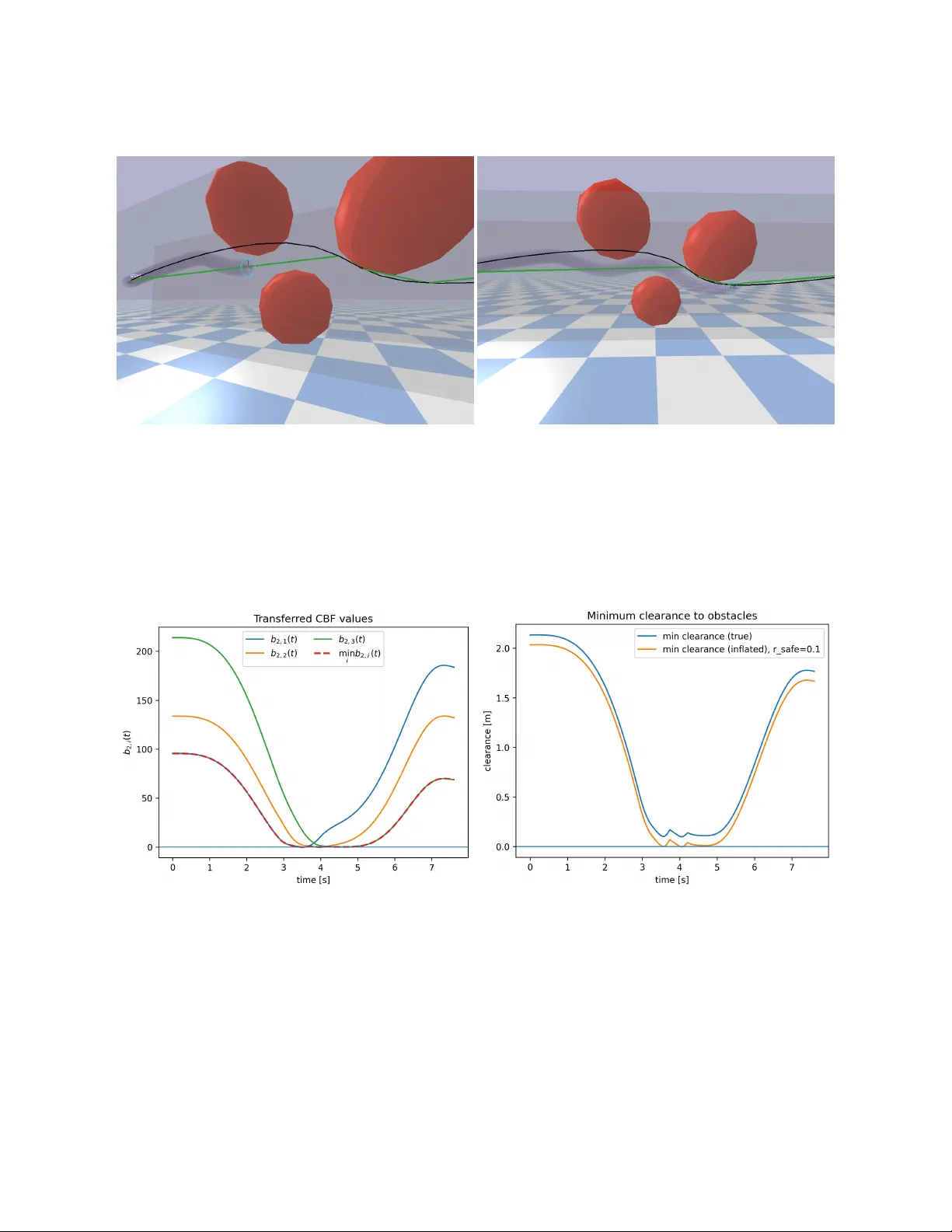
On transferring safety certificates across dynamical systems Nikolaos Bousias 1 , Charalampia Stamouli 1 , Anastasios Tsiamis 2 , and George P appas 1 1 GRASP Lab, Uni versity of Pennsylv ania 2 Automatic Control Laboratory , ETH Zürich Abstract Control barrier functions (CBFs) provide a powerful tool for enforcing safety constraints in control systems, but their direct application to complex, high-dimensional dynamics is often challenging. In many settings, safety certificates are more naturally designed for simplified or alternati ve system models that do not exactly match the dynamics of interest. This paper addresses the problem of transferring safety guarantees between dynamical systems with mismatched dynamics. W e propose a transferred control barrier function (tCBF) framework that enables safety constraints defined on one system to be systematically enforced on another system using a simulation function and an explicit margin term. The resulting transferred barrier accounts for model mismatch and induces a safety condition that can be enforced on the tar get system via a quadratic-program-based safety filter . The proposed approach is general and does not require the two systems to share the same state dimension or dynamics. W e demonstrate the effecti veness of the frame work on a quadrotor na vigation task with the transferred barrier ensuring collision av oidance for the target system, while remaining minimally in vasi ve to a nominal controller . These results highlight the potential of transferred control barrier functions as a general mechanism for enforcing safety across heterogeneous dynamical systems. 1 Intr oduction As autonomous systems become increasingly prev alent across robotics, aerospace, and industrial automa- tion, ensuring their safe operation remains a fundamental challenge. Control Barrier Functions (CBFs) hav e emerged as a powerful mathematical framew ork for enforcing safety constraints in real-time control systems [1, 2]. By encoding safety requirements as forward-in v ariant sets, CBFs enable the synthesis of minimally in vasi ve safety filters that can be integrated with arbitrary nominal controllers while providing formal guarantees of collision av oidance and constraint satisfaction. Despite their theoretical elegance and practical success, a significant gap exists between the abstract models used for safety analysis and the physical systems on which these guarantees must hold. Safety spec- ifications are often most naturally expressed and verified on simplified, nominal models—such as single or double integrators—that capture essential system dynamics while remaining tractable for formal verifica- tion. Ho wev er , deploying these safety guarantees on actual robotic platforms introduces substantial com- plexity: nonlinear dynamics, underactuation, geometric constraints, and actuator limitations all conspire to in v alidate safety certificates deriv ed from idealized models. The classical approach to bridging this gap relies on approximate bisimulation and simulation relations, which ha ve prov en instrumental in hierarchical verification and abstraction-based control synthesis [3, 4, 5]. These relations formalize the notion that one system (the concrete, physical system) can approximately reproduce the behavior of another (the abstract, nominal system). While simulation relations have been successfully applied to verify temporal logic specifications [6] and synthesize correct-by-construction con- trollers [7], their application to safety-critical control via CBFs remains relativ ely unexplored. Existing 1 CBF synthesis methods typically require designing barrier functions directly on the full-order nonlinear system [8, 9], which can be computationally prohibiti ve or require significant domain expertise. Recent work has begun to address the transferability of safety specifications across system abstractions. The concept of backup barrier functions [10] and the composition of multiple CBFs [11] pro vide mecha- nisms for handling complex safety requirements, while learning-based approaches [12, 13, 14] attempt to discov er CBF candidates for high-dimensional systems. Howe ver , these methods do not explicitly le verage the relationship between abstract and concrete system models, potentially discarding v aluable structure that could simplify the synthesis problem. Contributions In this paper , we develop a formal framework for transferring Control Barrier Functions from abstract sys- tems to concrete systems linked by simulation relations. Our key contrib utions are summarized below: 1. T ransfer construction: W e propose a transferred control barrier function (tCBF) formulation that enables safety certificates designed on an abstract dynamical model to be systematically enforced on a higher-dimensional nonlinear system using a simulation function and an e xplicit margin term. 2. F ormal guarantees & design guidelines: W e prov e that with appropriate design of the margin func- tion, the transferred safety certificates are valid for the new system, thereby inheriting safety guaran- tees. W e provide explicit conditions for selecting the margin function, including closed-form solutions for common cases. These guidelines enable practical implementation without requiring exhausti ve numerical optimization. W e apply the proposed framework to a quadrotor navig ating a cluttered three-dimensional en vironment using a double-inte grator abstraction, demonstrating how safety can be transferred from a simple abstract model to full nonlinear quadrotor dynamics. Our frame work addresses a critical gap in compositional safety verification: it allows practitioners to deriv e safety specifications on tractable abstract models while pro- viding rigorous guarantees when deployed on complex physical systems. This is particularly relev ant for modern robotic platforms where computing resources at deployment time are limited, making it desirable to perform complex safety synthesis of fline on simplified models. 2 Pr eliminaries Consider dynamical systems Σ 1 : ˙ x 1 ( t ) = f 1 ( x 1 ( t ) , u 1 ( t )) ∈ X ( X 1 × U 1 ) , y 1 ( t ) = g 1 ( x 1 ( t )) Σ 2 : ˙ x 2 ( t ) = f 2 ( x 2 ( t ) , u 2 ( t )) ∈ X ( X 2 × U 2 ) , y 2 ( t ) = g 2 ( x 2 ( t )) with states x 1 ∈ X 1 , x 2 ∈ X 2 , inputs u 1 ∈ U 1 , u 2 ∈ U 2 , outputs on the same space y 1 , y 2 ∈ Y and X ( X i ) denoting the generated vector fields. For a continuously dif ferentiable function b i : X 1 , 2 → R , its Lie deriv ativ e along f 1 , 2 is denoted by L u i 7→ f i b i ( x i ) := ⟨∇ b i ( x i ) ⊤ , f i ( x i , u i ) ⟩ A function α : R ≥ 0 → R ≥ 0 is class- K if it is continuous, strictly increasing, and α (0) = 0 . It is K ∞ if, in addition, α ( s ) → ∞ as s → ∞ . 2 2.1 Control Barrier Functions Definition 1. A continuously dif fer entiable function b i : X i → R is a valid Contr ol Barrier Function (CBF) for Σ i in the closed set S i := { x i ∈ X i : b i ( x i ) ≥ 0 } , if there e xists α b ∈ K such that: sup u i ∈ U i L u i 7→ f i b i ( x i ) ≥ − α b  b i ( x i )  ∀ x i ∈ X i (1) Under standar d r e gularity (e.g ., locally Lipschitz-bounded vector fields), any policy u i ∈ U i that enfor ces L u i ( t ) 7→ f i b i ( x i ( t )) ≥ − α b  b i ( x i ( t ))  ∀ x i ∈ X i , t ∈ R + r enders S i forwar d in variant, i.e. keeps the system safe. 2.2 Simulation functions and interfaces Definition 2. A continuously differ entiable function V : X 1 × X 2 → R ≥ 0 is a simulation function fr om system Σ 2 to system Σ 1 if, for some control interface F : X 1 × X 2 × U 2 → U 1 , ∀ ( x 1 , x 2 , u 2 ) ∃ : • a class- K ∞ function γ bounding an output mismatc h || y 1 − y 2 || Y ≤ γ ( V ( x 1 , x 2 ) (2) • a class- K ∞ function α V such that the decay inequality holds: ⟨∇ x 1 V ( x 1 , x 2 ) ⊤ , f 1 ( x 1 , F ( x 1 , x 2 , u 2 ) ⟩ + ⟨∇ x 2 V ( x 1 , x 2 ) ⊤ , f 2 ( x 2 , u 2 ) ⟩ ≤ − α V  V ( x 1 , x 2 )  (3) For simplicity we drop the time dependence from the notation and lea ve it implied. 2.3 Witness map and the pushf orward on the witness graph A (local) witness map Π : X 2 → X 1 assigns an element from X 1 to x 2 via Π( x 2 ) ∈ arg min x 1 V ( x 1 , x 2 ) (4) W e assume that Π is continuously differentiable on a neighborhood of interest and that the minimizer is unique there. Under these conditions, first-order optimality yields ∇ x 1 V  Π( x 2 ) , x 2  = 0 (5) W e define the witness graph G := { ( x 1 , x 2 ) ∈ X 1 × X 2 : x 1 = Π( x 2 ) } with its tangent space at (Π( x 2 ) , x 2 ) denoted T (Π( x 2 ) ,x 2 ) G = { ( D Π( x 2 ) v , v ) : v ∈ T x 2 X 2 } . The pair of vector fields  f 1 ( x 1 , F ( x 1 , x 2 , u 2 )) , f 2 ( x 2 , u 2 )  is tangent to G at (Π( x 2 ) , x 2 ) if D Π( x 2 )  f 2 ( x 2 , u 2 )  = f 1  Π( x 2 ) , F  Π( x 2 ) , x 2 , u 2   (6) When (6) holds, the chain rule collapses to a directional deri vati ve in the Σ 1 dynamics with the interface: ⟨∇ b 1  Π( x 2 )  ⊤ , D Π( x 2 ) f 2 ( x 2 , u 2 ) ⟩ = L F  Π( x 2 ) ,x 2 ,u 2  7→ f 1 b 1  Π( x 2 )  (7) which is the pushforwar d identity on the witness graph . The witness graph formalizes the notion that each concrete state is paired with its closest abstract representativ e under the simulation metric. When the joint dynamics are tangent to this graph, ev olution of the concrete system can be interpreted through the abstract dynamics via a pushforward relationship. This observ ation allows Lie deri v ativ es on the concrete system to be related directly to those on the abstract system, forming the backbone of the safety transfer analysis. 3 3 T ransferring safety certificates acr oss dynamical systems The central challenge in transferring safety certificates is that the abstract and concrete systems generally e volv e on different state spaces and under different dynamics. Even when their behaviors are related through a simulation function, enforcing a barrier constraint directly on the concrete system may fail due to mismatch between the two trajectories. Our approach compensates for this mismatch by shrinking the abstract safe set according to the simu- lation error . Intuiti vely , if the concrete state is close (in the sense of the simulation function) to an abstract safe state, then safety can still be guaranteed, provided a suitable margin is enforced. This idea motiv ates the follo wing construction. Definition 3. Consider a valid CBF for system Σ 1 , b 1 : X 1 → R of Definition 1. F or some simulation function V : X 1 × X 2 → R ≥ 0 with contr ol interface F : X 1 × X 2 × U 2 → U 1 fr om Definition 2, we define the transferred Control Barrier Function (t-CBF) b 2 : X 2 → R fr om Σ 1 on Σ 2 : b 2 ( x 2 ) := b 1  Π( x 2 )  − ϕ  V (Π( x 2 ) , x 2 )  , ϕ ∈ K ∞ (8) Definition 4. F or V : X 1 × X 2 → R ≥ 0 and F : X 1 × X 2 × U 2 → U 1 (Definition 2) and induced witness map Π : X 2 → X 1 of (4), define the dynamics mismatch : δ ( x 2 , u 2 ) := D Π( x 2 ) [ f 2 ( x 2 , u 2 )] − f 1  Π( x 2 ) , F  Π( x 2 ) , x 2 , u 2   (9) Assumption 1. One of the following hypotheses stands. H1. Exact pushforwar d: If (6) holds, then δ ≡ 0 . H2. Stationarity: If (5) holds ∃ γ ∈ K ∞ with |∇ Π b 1 (Π( x 2 )) ⊤ δ ( x 2 , u 2 ) | ≤ γ  V (Π( x 2 ) , x 2 )  H3. Gener al appr oximate pushforwar d: if ∃ Γ ∈ K ∞ with     ∇ Π b 1  Π( x 2 )  − dϕ  V (Π( x 2 ) , x 2 )  ∇ x 1 V (Π( x 2 ) , x 2 )  ⊤ δ ( x 2 , u 2 )    ≤ Γ  V (Π( x 2 ) , x 2 )  W e now analyze how the transferred barrier ev olves along trajectories of the concrete system. The ke y idea is to decompose the time deri vati v e of the transferred barrier into the follo wing components: i) a term corresponding to the abstract CBF dynamics ii) a term inherited from the simulation function decay iii) a residual mismatch term capturing imperfect pushforw ard By bounding each component separately , we obtain a differential inequality that isolates the role of the margin function in restoring the standard CBF condition. Lemma 1. Suppose b 1 is a valid CBF for Σ 1 with α b ∈ K , and V is a simulation function with decay α V ∈ K ∞ and interface F , then : ˙ b 2 ( x 2 , u 2 ) ≥ − α b  b 1 (Π( x 2 ))  + dϕ  V (Π( x 2 ) , x 2 )  α V  V (Π( x 2 ) , x 2 )  − r  V (Π( x 2 ) , x 2 )  wher e r ∈ K ∞ under Assumption 1 and ∀ x 2 , u 2 . Pr oof. Differentiating the t-CBF b 2 along trajectories of Σ 2 yields, by the chain rule, d dt b 2 ( x 2 ) = ⟨∇ b 1  Π( x 2 )  ⊤ , D Π( x 2 )  f 2 ( x 2 , u 2 )  ⟩ − dϕ  V (Π( x 2 ) , x 2 )   ⟨∇ x 1 V  Π( x 2 ) , x 2  ⊤ , D Π( x 2 ) [ f 2 ( x 2 , u 2 )] ⟩ + ⟨∇ x 2 V  Π( x 2 ) , x 2  ⊤ , [ f 2 ( x 2 , u 2 )] ⟩  (10) 4 Lemma 1 sho ws that the transferred barrier satisfies a relaxed CBF condition, where violation of the abstract barrier constraint is compensated by decay of the simulation function and the margin deriv ati ve. The re- maining task is therefore to choose the margin function so that these additional terms dominate the abstract barrier gro wth, recovering a standard CBF inequality on the concrete system. From the optimality condition of the witness map (5) ∇ x 1 V  Π( x 2 ) , x 2  = 0 , thus the second line in 10 is simplified. W e retain it in the proof below to accommodate scenarios where only approximate optimality is av ailable. Adding/subtract f 1 (Π , F ) in 10 where ver D Π[ f 2 ] appears: d dt b 2 ( x 2 ) = D ∇ Π b 1 (Π( x 2 )) ⊤ , f 1  Π( x 2 ) , F  Π( x 2 ) , x 2 , u 2  E | {z } CBF term on Σ 1 − dϕ ( V (Π( x 2 ) , x 2 )) h ⟨∇ x 1 V (Π( x 2 ) , x 2 ) ⊤ , f 1  Π( x 2 ) , F  Π( x 2 ) , x 2 , u 2   ⟩ + ⟨∇ x 2 V (Π( x 2 ) , x 2 ) ⊤ , f 2 ( x 2 , u 2 ) ⟩ i | {z } simulation term +  ∇ Π b 1  Π( x 2 )  − dϕ  V (Π( x 2 ) , x 2 )  ∇ x 1 V (Π( x 2 ) , x 2 )  ⊤ δ ( x 2 , u 2 ) | {z } mismatch term (11) For the CBF term on Σ 1 , if b 1 is a v alid CBF for Σ 1 , then L u 1 7→ f 1 b 1 ( x 1 ) ≥ α b ( b 1 ( x 1 )) , ∀ x 1 , u 1 . Evaluating at x 1 = Π( x 2 ) with u 1 = F (Π( x 2 ) , x 2 , u 2 ) yields: ⟨∇ Π b 1 (Π( x 2 )) ⊤ , f 1  Π( x 2 ) , F  Π( x 2 ) , x 2 , u 2   ⟩ ≥ α b  b 1  Π( x 2 )   For the simulation term, the decay (2) e v aluated at ( x 1 , x 2 ) = (Π( x 2 ) , x 2 ) yields: ⟨∇ x 1 V (Π( x 2 ) , x 2 ) ⊤ , f 1  Π( x 2 ) , F  Π( x 2 ) , x 2 , u 2   ⟩ + ⟨∇ x 2 V (Π( x 2 ) , x 2 ) ⊤ , f 2 ( x 2 , u 2 ) ⟩ ≤ − α V  V  Π( x 2 )   Combining (11) with CBF/Simulation bounds and Assumption 1 yields the lo wer bound of Lemma 1. W e now isolate a design condition on ϕ that con verts Lemma 1 into a standard CBF inequality . Assumption 2. F or α V , α b , r : [0 , ∞ ) → [0 , ∞ ) be (extended) K -class functions, i.e ., continuous, strictly incr easing, and α V (0) = α b (0) = r (0) = 0 ∃ ϕ ∈ K ∞ such that ϕ ′ ( s ) α V ( s ) ≥ α b  ϕ ( s )  + r ( s ) , ∀ s ≥ 0 . Intuiti vely , the margin function must grow fast enough so that the decay of the simulation function of fsets both the abstract barrier contraction and any residual dynamics mismatch. This condition depends only on scalar comparison functions, making margin synthesis independent of the system dimension. Theorem 1. F ix s 0 > 0 and ϕ ( s 0 ) = η ≥ 0 . Assume that for each compact K ⊂ [0 , ∞ ) the map x 7→ α b ( x ) is locally Lipschitz on K . Let y : [ s 0 , ∞ ) → [0 , ∞ ) be the unique Carathéodory solution of ˙ y ( s ) = λ ( s, y ( s )) = α b ( y ( s )) + r ( s ) α V ( s ) , y ( s 0 ) = η . (12) If ϕ is absolutely continuous, satisfies the ODE inequality for a.e. s ≥ s 0 , and ϕ ( s 0 ) ≥ η , then ϕ ( s ) ≥ y ( s ) , ∀ s ≥ s 0 . (13) In particular , among all ϕ ∈ K ∞ satisfying the the ODE inequality , the solution y ( s ) is pointwise minimal. Pr oof. Appendix C. 5 Since s 7→ r ( s ) /α V ( s ) is locally integrable on [ s 0 , ∞ ) , because r , α V ∈ K ∞ , and if a b ∈ K ∞ is locally Lipschitz (common), then by Picard–Lindelöf lemma (applies the Banach fixed-point theorem to Picard iterations) for the ODE 12 there al ways exists a unique solution in [ s 0 , s 0 + ϵ ] , s 0 , ϵ ∈ R + , recov ered by the Picard iterations: y κ +1 ( s ) = η + Z s s 0 a b ( y κ ( τ )) + r ( τ ) a V ( τ ) dτ s ≥ s 0 , y 0 = η (14) In the case of perfect dynamics recapturing, i.e. r ≡ 0 , Assumption 2 can be interpreted as a separation condition between safety enforcement and model mismatch. For some reference points ˆ x, ˆ s ∈ R + , defining F ( x ) := R x ˆ x 1 a b ( u ) du and G ( x ) := R s ˆ s 1 a V ( τ ) dτ , yields separated solution y ( s ) = F − 1 ( F ( η )+ G ( s ) − G ( s 0 )) . Since extended K functions are strictly increasing, α b is injecti ve, and F , G are strictly increasing wherev er the integrals are well-defined, so F − 1 is well-defined on its image. Proposition 1. Let α b ( s ) = c b s and α V ( s ) = c V s with c b , c V > 0 . F ix s 0 > 0 and ϕ ( s 0 ) = η ≥ 0 . Then the Carathéodory solution of the comparison ODE 12 admits the r epresentation y ( s ) =  s s 0  c b c V η + 1 c V s c b c V Z s s 0 τ − c b c V − 1 r ( τ ) dτ , s ≥ s 0 . (15) In particular , if r ≡ 0 , then y ( s ) = η  s s 0  c b c V . (16) If r is linear , i.e. r ( s ) = c r s with c r ≥ 0 , then y ( s ) =        η  s s 0  λ + c r c V (1 − λ )  s 1 − λ − s 1 − λ 0  , λ  = 1 , η  s s 0  + c r c V s log  s s 0  , λ = 1 . (17) Pr oof. Appendix D. Theorem 2. Let Assumptions 1 and 2 stand. There exists a class- K function e α : R → R suc h that along trajectories of Σ 2 it stands that d dt b 2 ( x 2 , u 2 ) + e α  b 2 ( x 2 )  ≥ 0 , ∀ x 2 ∈ X 2 , u 2 ∈ U ∈ , thus, any feedback enfor cing this inequality r enders S 2 := { x 2 | b 2 ( x 2 ) ≥ 0 } forwar d in variant, i.e., b 2 is a valid CBF for Σ 2 . Pr oof. Using b 1  Π( x 2 )  = b 2 ( x 2 ) + ϕ  V (Π( x 2 ) , x 2 )  in (8) and Assumption 2, ˙ b 2 ( x 2 ) ≥ − α b  b 2 ( x 2 ) + ϕ ( V (Π( x 2 ) , x 2 ))  +  dϕ ( V (Π( x 2 ) , x 2 )) α V ( V (Π( x 2 ) , x 2 )) − r ( V (Π( x 2 ) , x 2 ))  | {z } ≥ α b ( ϕ ( V (Π( x 2 ) ,x 2 ))) Define the comparison function e α ( s ) := sup r ≥ 0  α b ( s + r ) − α b ( r )  , s ≥ 0 . Since α b ∈ K : (i) e α (0) = 0 ; (ii) For s 2 > s 1 , α b ( s 2 + r ) − α b ( r ) > α b ( s 1 + r ) − α b ( r ) for all r , so after taking the supremum, e α ( s 2 ) > e α ( s 1 ) ; (iii) Continuity follo ws from monotonicity and continuity of α b ∈ K ∞ . Hence e α ∈ K and α b ( s + r ) − α b ( r ) ≤ e α ( s ) for all r , s ≥ 0 . Therefore, ˙ b 2 ≥ − e α  b 2  . Forward inv ariance of S 2 then follows from standard CBF arguments. Remark 1. F or the case exact push-forward, i.e. no dynamics miss-match δ = 0 , System 1 constitutes a r educed-or der model of System 2 and the t-CBF is similar to [15, 16]. Theorem 2 establishes that safety verified on an abstract model can be enforced on a more complex con- crete system without redesigning the barrier function. The only additional requirement is the construction of a mar gin that quantifies simulation error . As a result, safety synthesis and safety enforcement can be cleanly decoupled across system representations. 6 Safe optimal control with tCBF-QP This section describes how the transferred Control Barrier Function (tCBF) is enforced in real time via a quadratic program (QP) on the target system Σ 2 . Substituting Lemma 1 into Definition 8 yields the constraint ⟨∇ b 1 (Π( x 2 )) , D Π( x 2 ) f 2 ( x 2 , u 2 ) ⟩ − ϕ ′ ( V ) ⟨∇ x 2 V (Π( x 2 ) , x 2 ) , f 2 ( x 2 , u 2 ) ⟩ ≥ − α e ( b 2 ( x 2 )) + r ( V (Π( x 2 ) , x 2 )) . (18) For control-af fine tar get dynamics f 2 ( x 2 , u 2 ) = f 2 , 0 ( x 2 ) + f 2 , 1 ( x 2 ) u 2 , the constraint (18) is action-affine and thus suitable for quadratic programming. Let u nom ( x 2 ) denote an arbitrary nominal controller . The tCBF-based safety filter is gi ven by the quadratic program u ⋆ 2 ( x 2 ) = arg min u 2 ∈ U 2 ∥ u 2 − u nom ( x 2 ) ∥ 2 s.t. A ( x 2 ) u 2 ≥ b ( x 2 ) (19) where, for ¯ x 1 ≜ Π( x 2 ) , ¯ V ≜ V ( ¯ x 1 , x 2 ) and ϕ ′ ≜ dϕ ( ¯ V ) , A ( x 2 ) :=  ∇ b 1 ( ¯ x 1 )  ⊤ D Π( x 2 ) f 2 , 1 ( x 2 ) − ϕ ′ ( V ( ¯ x 1 , x 2 )) ∇ x 2 V ( ¯ x 1 , x 2 ) ⊤ f 2 , 1 ( x 2 ) b ( x 2 ) := − α e  b 2 ( x 2 )  + r ( ¯ V ) −  ∇ b 1 ( ¯ x 1 )  ⊤ D Π( x 2 ) f 2 , 0 ( x 2 ) + ϕ ′ ( V ( ¯ x 1 , x 2 )) ∇ x 2 V ( ¯ x 1 , x 2 ) ⊤ f 2 , 0 ( x 2 ) , Any solution u ⋆ 2 renders the set S 2 = { x 2 ∈ X 2 | b 1  Π( x 2 )  − ϕ  V (Π( x 2 ) , x 2 )  ≥ 0 } forward in v ariant. Algorithm 1 tCBF-QP Safety Filter Require: Current state x 2 , nominal input u nom ( x 2 ) Ensure: Safe control input u ⋆ 2 1: Compute witness state Π( x 2 ) ∈ arg min x 1 V ( x 1 , x 2 ) 2: Ev aluate V ← V (Π( x 2 ) , x 2 ) 3: Compute mar gin terms ϕ ( V ) and ϕ ′ ( V ) 4: Ev aluate gradients ∇ b 1 (Π( x 2 )) , D Π( x 2 ) , and ∇ x 2 V (Π( x 2 ) , x 2 ) 5: F orm the affine constraint (18) 6: Solv e the quadratic program: min u 2 ∈ U 2 ∥ u 2 − u nom ∥ 2 s.t. ˙ b 2 + α e ( b 2 ) ≥ 0 7: Apply u ⋆ 2 4 Experiments W e consider the problem of safely na vigating a quadrotor through a static, obstacle-cluttered en vironment from a given initial position p 0 ∈ R 3 to a desired target p T ∈ R 3 while av oiding collisions. Obstacles O = { 1 , .., N } are modeled as spheres with centers c i ∈ R 3 and inflated radii ρ i > 0 . Let Σ 1 be the 3D double integrator on X 1 = R 3 × R 3 with dynamics ˙ p 1 = v 1 , ˙ v 1 = u 1 , , y 1 = p 1 , where x 1 = ( p 1 , v 1 ) and u 2 ∈ R 3 is the abstract acceleration input. Let Σ 2 be the standard rigid-body quadrotor on X 2 = R 3 × R 3 × S O (3) × R 3 with dynamics: ˙ x 2 = d dt     p 2 v 2 R Ω     =     v 2 − g e 3 + 1 m f R e 3 R [Ω] ∧ J − 1  M − Ω × ( J Ω)      7 and y 2 = p 2 , m > 0 , g > 0 , e 3 = [0 0 1] ⊤ , inputs u 2 = ( f , M ) ∈ R × R 3 , and [ · ] ∧ : R 3 → so ( 3 ) is the hat operator . 4.1 Policy interface, simulation function & witness map Define the error states e p = p 2 − p 1 , e v = v 2 − v 1 and consider the control interface F ( x 1 , x 2 , u 2 ) = ( f m Re 3 − g e 3 ) + K p e p + K v e v for K p , K v ∈ R 3 × 3 such that A =  0 I − K p − K v  is Hurwitz stable. For some Q ≻ 0 let P ≻ 0 be the unique solution of the L yapunov equation A T P + PA = Q . Define the continuously differentiable positi ve semi-definite candidate simulation function V ( x 1 , x 2 ) := z ⊤ P z ≥ 0 , z = [ e p , e v ] T ∈ R 6 with witness map Π( x 2 ) = argmin x 1 V ( x 1 , x 2 ) = [ p 2 , v 2 ] T satisfying the first- order optimality condition ∇ x 1 V (Π( x 2 ) , x 2 ) = 0 . The candidate simulation function is valid according to Definition 2 since ∥ y 2 − y 1 ∥ = ∥ e p ∥ ≤ γ ( V ( x 1 , x 2 )) for γ ( s ) = 1 p λ min ( P ) √ s ∈ K ∞ and from the error dynamics the decay inequality is ˙ V ( x 1 , x 2 ) = − z T Q z ≤ − λ min ( Q ) ∥ z ∥ 2 ≤ − α V ( V ( x 1 , x 2 )) for α V ( s ) = λ min ( Q ) λ max ( P ) s ∈ K ∞ . The dynamics mismatch, then, is δ ( x 2 , u 2 ) := D Π( x 2 ) [ f 2 ( x 2 , u 2 )] − f 1  Π( x 2 ) , F  Π( x 2 ) , x 2 , u 2   ≡ 0 satisfying Assumption 1. 4.2 T ransfering safety certificates from Σ 1 to Σ 2 Define the distance-squared safety function h i ( x 1 ) := ∥ p 1 − c i ∥ 2 − ρ 2 i , ∀ i ∈ O . F or Σ 1 the CBF candidate h i has relati ve degree 2 and safety is enforced via an exponential CBF condition ¨ h i ( x 1 ) + k b, 1 ˙ h i ( x 1 ) + k b, 2 h i ( x 1 ) ≥ 0 which is equiv alent to enforcing a zeroing CBF b 1 ,i ( x 1 ) := ˙ h i ( x 1 ) + k b, 1 h i ( x 1 ) satisfying ˙ b 1 ,i ( x 1 , u 1 ) ≥ − α b ( b 1 ,i ( x 1 )) for α b ( s ) := k b, 2 s ∈ K ∞ , k b, 2 , k b, 2 > 0 , yielding an affine constraint on the abstract control input u 1 . T o deploy this safety certificate on a quadrotor with nonlinear, underactuated dynamics, we construct the candidate tCBF from 8. W ith an appropriate choice of ϕ satisfying the ODE inequality of Assumption 2, the function b 2 ,i is a v alid control barrier function for the quadrotor , enabling safe navigation via real-time quadratic programming according to Algorithm 1. From Proposition 1, since α V , α b ∈ K ∞ are linear and δ ≡ 0 , ϕ ( s ) ≥ ϕ ( s 0 )  s s 0  k b, 2 λ max ( P ) λ min ( Q ) for any ϕ ( s 0 ) , s 0 ∈ R + . 4.3 Nominal quadrotor policy design The transferred control barrier function is implemented as a safety filter that minimally modifies a nominal quadrotor controller . The nominal polic y is designed to generate dynamically feasible trajectories that dri ve the vehicle from a given start position to a target while respecting quadrotor dynamics in the absence of safety constraints. Our nominal control pipeline consists of motion planning, trajectory optimization, and geometric tracking control. Initially , a sampling-based planner using RR T ∗ [17] computes a collision-free geometric path from the start to the goal in the obstacle-cluttered en vironment. The resulting sequence of waypoints provides a feasible but non-smooth reference path. The discrete RR T ∗ path is con verted into a smooth, time-parameterized trajectory by solving a minimum-snap trajectory optimization problem [18]. Specifically , utilizing the differential flatness of the quadrotor , we generate a piecewise polynomial trajectory p d ( t ) by minimizing the snap ov er the trajectory min p d ( t ) Z T 0     d dt 4 p d ( t )     2 dt 8 Figure 1: Instances of the quadrotor trajectory in an obstacle en vironment. Red spheres denote obstacles, the green curve shows the RR T* path, and the black curve sho ws the nominal minimum-snap trajectory incurring collisions. Semi-transparent purple spheres indicate the tCBF-QP trajectory . Figure 2: (Left) Evolution of the transferred control barrier functions associated with each obstacle. The minimum transferred barrier value is shown by the dashed curve. As the quadrotor approaches obstacles, the transferred barriers decrease and become acti ve near zero, demonstrating enforcement of safety at the concrete system lev el despite abstraction mismatch. (Right) Minimum obstacle clearance along the trajec- tory . The true geometric clearance remains strictly positive, confirming collision av oidance. The inflated clearance used in the abstract barrier construction is sho wn for reference, illustrating the additional safety margin imposed by the transferred CBF . 9 subject to continuity constraints on position and its deriv ati ves up to snap, waypoint interpolation con- straints, and boundary conditions on position, velocity , and acceleration for desired yaw aligned with the quadrotor’ s velocity , i.e. ψ d ( t ) = acrtan ( v 2 ,y , v 2 ,x ) . This yields a smooth reference trajectory p d ( t ) with associated desired velocity ˙ p d ( t ) , acceleration ¨ p d ( t ) , and jerk p (3) d ( t ) . Finally , the quadrotor tracks the ref- erence trajectory using an S E (3) -geometric controller [19]. The desired total force vector is computed as F d ( t ) = m ( ¨ p d ( t ) + g e 3 ) − ¯ k p ( p 2 ( t ) − p d ( t )) − ¯ k v ( v ( t ) − ˙ p d ( t )) , for some ¯ k p , ¯ k v > 0 . The commanded thrust is f nom ( t ) = F d ( t ) ⊤ R ( t ) e 3 ∈ R and the desired body z -axis is defined as b z ,d ( t ) = F d ( t ) ∥ F d ( t ) ∥ . T ogether with the desired yaw direction, this defines a desired rotation matrix R d ( t ) = [ b x,d , b y ,d , b z ,d ] ∈ S O (3) for σ ( t ) = [cos( ψ d ( t )) , sin( ψ d ( t )) , 0] ⊤ , b y ,d ( t ) = b z,d ( t ) × σ ( t ) ∥ b z,d ( t ) × σ ( t ) ∥ , b x,d ( t ) = b y ,d ( t ) × b z ,d ( t ) . Let e R ( t ) = 1 2 [ R ⊤ d ( t ) R ( t ) − R ⊤ ( t ) R d ( t )] ∨ and e Ω ( t ) = Ω( t ) − ˙ R d ( t ) denote the attitude and angular velocity error states, respecti vely , with ¯ k R , ¯ k Ω > 0 control gains and [ · ] ∨ : so ( 3 ) → R 3 denoting the vee operator . The attitude control moment is then M nom ( t ) = J ( − ¯ k R e R ( t ) − ¯ k Ω e Ω ( t )) ∈ R 3 , resulting to nominal input u nom ( t ) = ( f nom ( t ) , M nom ( t )) . This nominal controller achiev es aggressiv e trajectory tracking in free space, while the tCBF-based quadratic program modifies u nom ( t ) only when required to ensure obstacle av oidance. The safety-filtered thrust-moment actions are con verted to rotor actuation ω 2 nom ( t ) =     k F k F k F k F 0 k F l 0 − k F l − k F l 0 k F l 0 − k M k M − k M k M     − 1  f nom ( t ) M nom ( t )  ∈ R 4 4.4 Results & Discussion W e now discuss the behavior of the proposed tCBF-QP safety filter and e valuate its ability to enforce safety on the full quadrotor dynamics while minimally modifying the nominal controller . T rajectory-level behavior : Figure 1 shows representativ e snapshots of the quadrotor trajectory in the obstacle environment. The green curve corresponds to the collision-free geometric path computed by RR T*, while the black curve denotes the nominal minimum-snap trajectory obtained from trajectory optimization and tracked by the SE(3) controller in the absence of safety constraints. As expected, the nominal trajectory intersects the obstacle regions and would result in collisions. When the transferred control barrier function is enforced via the quadratic program, the resulting trajectory (visualized by the semi-transparent purple spheres) deviates locally from the nominal trajectory in the vicinity of obstacles while remaining close to it else where. This demonstrates that the tCBF-QP acts as a minimally inv asi ve safety filter: control modifications occur only when the system approaches the boundary of the transferred safe set, and nominal performance is largely preserved aw ay from safety-critical regions. The quadrotor is able to pass through narro w regions between obstacles while remaining within the transferred safety en v elope, highlighting the non-conserv ativ e nature of the proposed approach. T ransferred barrier activation : The e volution of the transferred control barrier functions associated with each obstacle is shown in Figure 2 (left). Each curve corresponds to a transferred barrier , while the dashed curve represents their pointwise minimum. As the quadrotor approaches the obstacles, the corresponding transferred barrier v alues decrease and become activ e near zero, indicating enforcement of the safety con- straint at the concrete system lev el. After the point of closest approach, the barrier values increase again as the system moves aw ay from the obstacles. This behavior is consistent with the theoretical analysis in Sec- tion 3: although the safety certificate is synthesized on the abstract double-integrator model, the transferred barrier correctly identifies safety-critical situations for the full quadrotor dynamics and activ ates only when required. Collision a voidance : Figure 2 (right) reports the minimum distance between the quadrotor and the nearest 10 obstacle over time. The true geometric clearance remains strictly positi ve throughout the trajectory , con- firming collision avoidance for the full nonlinear system. For comparison, the inflated clearance used in the abstract barrier construction is also sho wn. Notably , the inflated clearance briefly approaches zero near the point of closest approach, reflecting the conserv atism introduced to account for abstraction mismatch. Ne vertheless, the true clearance remains positive, indicating that the transferred barrier successfully com- pensates for model mismatch while preserving physical safety . This observation empirically validates the role of the margin function ϕ in shrinking the abstract safe set to obtain a sound safety certificate on the concrete system. T aken together , the results demonstrate that the proposed tCBF framew ork enables safety certificates synthesized on a simplified abstract model to be enforced on a high-dimensional, underactuated quadrotor system. The transferred barrier acti v ates precisely in safety-critical situations, ensures collision a voidance in the concrete system, and results in only localized deviations from the nominal trajectory . These find- ings support the theoretical guarantees established in Section 3 and illustrate the practical ef fecti veness of transferred control barrier functions for safe autonomous navig ation under model mismatch. 5 Conclusions & Futur e work This paper introduced a transferred control barrier function (tCBF) framework for enforcing safety guaran- tees using safety certificates synthesized on simpler abstract models. By lev eraging a simulation function and an appropriate margin term, safety constraints defined on an abstract system can be systematically trans- ferred to ne w dynamical systems and enforced through a QP-based safety filter . Numerical experiments on a quadrotor navig ating a cluttered three-dimensional en vironment demonstrated that the transferred barrier acti vates precisely in safety-critical situations, ensures collision av oidance for the full nonlinear system, and remains minimally in v asiv e away from obstacles. A ke y challenge in applying transferred barrier functions in practice is the construction of suitable simu- lation functions and policy interf aces, which can be dif ficult to deriv e analytically for complex systems. An important direction for future work is therefore to make these components learnable from data. Learning simulation functions and abstraction interfaces could significantly broaden the applicability of tCBFs and enable safety transfer in settings where accurate analytical models are unav ailable. 11 A ppendix The follo wing appendices collect standard technical results that support the main construction and are in- cluded for completeness. A: Constructing Π and verifying (5) Suppose V ( · , x 2 ) is strictly con ve x and C 2 on X 1 for each fix ed x 2 and coercive. Then the ar gmin is unique, and the implicit function theorem applied to ∇ x 1 V ( x 1 , x 2 ) = 0 around any point with det( ∇ 2 x 1 V ) > 0 yields a C 1 mapping Π( x 2 ) . Equation (4) is precisely the first-order optimality condition. B: On the existence of ϕ satisfying Assumption 2 Under local Lipschitzness of the right-hand side of the ODE and positivity of α V on (0 , ∞ ) , the ODE has a unique maximal solution with ϕ ∈ K ∞ (strict increase follows from positivity; unboundedness follows from div ergence of the integral R ∞ d s α V ( s ) or by continuation of solutions). Any such solution satisfies the ordinary differential inequality as an equality; replacing equality with inequality preserves the result by monotonicity . C: Proof of Theor em 1 Pr oof. Rewrite the ODE inequality on [ s 0 , ∞ ) as ˙ ϕ ( s ) ≥ f ( s, ϕ ( s )) for a.e. s ≥ s 0 , with f the righ-hand side of the ODE inequality . Let y solv e (12). Define w ( s ) := ( y ( s ) − ϕ ( s )) + = max { y ( s ) − ϕ ( s ) , 0 } . F or a.e. s such that w ( s ) > 0 we ha ve y ( s ) > ϕ ( s ) , hence by monotonicity of α b , α b ( y ( s )) − α b ( ϕ ( s )) > 0 , and therefore ˙ y ( s ) − ˙ ϕ ( s ) = α b ( y ( s )) + r ( s ) α V ( s ) − ˙ ϕ ( s ) ≤ α b ( y ( s )) + r ( s ) α V ( s ) − α b ( ϕ ( s )) + r ( s ) α V ( s ) = α b ( y ( s )) − α b ( ϕ ( s )) α V ( s ) . Using local Lipschitzness of α b on bounded sets, there exists L > 0 (on any interval where y , ϕ remain bounded) such that | α b ( y ) − α b ( ϕ ) | ≤ L | y − ϕ | = Lw . Thus, for a.e. s , d ds w ( s ) ≤ L α V ( s ) w ( s ) . Since α V ( s ) > 0 for s ≥ s 0 > 0 and 1 /α V is locally integrable on [ s 0 , ∞ ) , Grönwall’ s inequality yields w ( s ) ≤ w ( s 0 ) exp  Z s s 0 L α V ( σ ) dσ  . But w ( s 0 ) = ( y ( s 0 ) − ϕ ( s 0 )) + = ( η − ϕ ( s 0 )) + = 0 by ϕ ( s 0 ) ≥ η , hence w ( s ) ≡ 0 and therefore y ( s ) ≤ ϕ ( s ) for all s ≥ s 0 . D: Proof of Pr oposition 1 Pr oof. With α b ( s ) = c b s and α V ( s ) = c V s , the ODE on [ s 0 , ∞ ) becomes, for s > 0 , c V s ϕ ′ ( s ) = c b ϕ ( s ) + r ( s ) , (20) 12 or equi valently ϕ ′ ( s ) − c b c V 1 s ϕ ( s ) = 1 c V r ( s ) s . (21) Let λ := c b /c V and consider the integrating factor µ ( s ) = s − λ , which is C 1 on [ s 0 , ∞ ) since s 0 > 0 . Multiplying both sides by µ ( s ) yields s − λ ϕ ′ ( s ) − λs − λ − 1 ϕ ( s ) = 1 c V s − λ − 1 r ( s ) , (22) and the left-hand side is the deri vati ve of s − λ ϕ ( s ) , i.e. d ds  s − λ ϕ ( s )  = 1 c V s − λ − 1 r ( s ) . (23) Integrating from s 0 to s ≥ s 0 and using ϕ ( s 0 ) = η giv es s − λ ϕ ( s ) = s − λ 0 η + 1 c V Z s s 0 τ − λ − 1 r ( τ ) dτ . (24) Multiplying by s λ yields the claimed representation, ϕ ( s ) =  s s 0  λ η + 1 c V s λ Z s s 0 τ − λ − 1 r ( τ ) dτ . (25) If r ≡ 0 , the integral term v anishes and ϕ ( s ) = η ( s/s 0 ) λ . If additionally r is linear, i.e. r ( s ) = c r s with c r ≥ 0 , then Z s s 0 τ − λ − 1 r ( τ ) dτ = c r Z s s 0 τ − λ dτ =        c r 1 − λ  s 1 − λ − s 1 − λ 0  , λ  = 1 , c r log  s s 0  , λ = 1 . (26) Substituting into the general formula yields, for λ  = 1 , ϕ ( s ) = η  s s 0  λ + c r c V (1 − λ )  s − s λ s 1 − λ 0  , (27) and for λ = 1 , ϕ ( s ) = η  s s 0  + c r c V s log  s s 0  . (28) E: Picking linear function ϕ Corollary 1. Let α b ( s ) = c b s and α V ( s ) = c V s with c b , c V > 0 . Assume ϕ ( s ) = c ϕ s for some constant c ϕ ∈ R . Then ϕ satisfies ϕ ′ ( s ) α V ( s ) = α b ( ϕ ( s )) + r ( s ) , ∀ s ≥ 0 , if and only if r ( s ) = c ϕ ( c V − c b ) s ∀ s ≥ 0 . In particular , if ϕ ∈ K and r ∈ K , then necessarily c ϕ > 0 and c V > c b , and in that case r ( s ) = c r s with c r = c ϕ ( c V − c b ) > 0 . 13 Pr oof. If ϕ ( s ) = c ϕ s , then ϕ ′ ( s ) = c ϕ . Substituting into the ODE gi ves c ϕ ( c V s ) = c b ( c ϕ s ) + r ( s ) , hence r ( s ) = c ϕ ( c V − c b ) s for all s ≥ 0 . Con versely , if r has this form, substitution shows the identity holds for all s ≥ 0 . The final claim follows since ϕ ∈ K implies c ϕ > 0 , and r ∈ K requires r ( s ) > 0 for s > 0 , i.e. c V − c b > 0 . Refer ences [1] A. D. Ames, S. Coogan, M. Egerstedt, G. Notomista, K. Sreenath, and P . T abuada, “Control barrier functions: Theory and applications, ” in Pr oceedings of the Eur opean Contr ol Confer ence (ECC) , 2019, pp. 3420–3431. [2] A. D. Ames, X. Xu, J. W . Grizzle, and P . T abuada, “Control barrier function based quadratic programs for safety critical systems, ” IEEE T ransactions on A utomatic Contr ol , v ol. 62, no. 8, pp. 3861–3876, 2017. [3] A. Girard and G. J. Pappas, “ Approximation metrics for discrete and continuous systems, ” IEEE T rans- actions on Automatic Contr ol , vol. 52, no. 5, pp. 782–798, 2007. [4] P . T abuada, V erification and Contr ol of Hybrid Systems: A Symbolic Appr oach . Springer Science & Business Media, 2009. [5] G. Reissig, A. W eber, and M. Rungger, “Feedback refinement relations for the synthesis of symbolic controllers, ” IEEE T ransactions on Automatic Contr ol , vol. 62, no. 4, pp. 1781–1796, 2017. [6] M. Kloetzer and C. Belta, “ A fully automated framework for control of linear systems from temporal logic specifications, ” IEEE T ransactions on Automatic Contr ol , vol. 53, no. 1, pp. 287–297, 2008. [7] M. Rungger and P . T abuada, “Computing robust controlled inv ariant sets of linear systems, ” IEEE T ransactions on Automatic Contr ol , vol. 62, no. 7, pp. 3665–3670, 2017. [8] W . Xiao and C. Belta, “Control barrier functions for systems with high relative degree, ” in Pr oceedings of the IEEE Confer ence on Decision and Contr ol (CDC) , 2019, pp. 474–479. [9] Q. Nguyen and K. Sreenath, “Exponential control barrier functions for enforcing high relativ e-degree safety-critical constraints, ” in Pr oceedings of the American Contr ol Confer ence (A CC) , 2016, pp. 322– 328. [10] A. D. Ames, J. W . Grizzle, and P . T abuada, “Control barrier function based quadratic programs with application to adaptiv e cruise control, ” in Pr oceedings of the IEEE Conference on Decision and Contr ol (CDC) , 2014, pp. 6271–6278. [11] U. Borrmann, L. W ang, A. D. Ames, and M. Egerstedt, “Control barrier certificates for safe swarm behavior , ” in IF AC W orkshop on Distributed Estimation and Contr ol in Networked Systems , 2015, pp. 68–73. [12] C. Dawson, Z. Qin, S. Gao, and C. Fan, “Safe control with learned certificates: A survey of neural lyapunov , barrier , and contraction methods, ” IEEE T ransactions on A utomatic Contr ol , 2023. 14 [13] A. Robey , H. Hu, L. Lindemann, H. Zhang, D. V . Dimarogonas, S. T u, and N. Matni, “Learning control barrier functions from expert demonstrations, ” in Pr oceedings of the IEEE Confer ence on Decision and Contr ol (CDC) , 2020, pp. 3717–3724. [14] N. Bousias, L. Lindemann, and G. Pappas, “Deep equiv ariant multi-agent control barrier functions, ” 2025. [Online]. A vailable: https://arxi v .org/abs/2506.07755 [15] T . G. Molnar , R. K. Cosner , A. W . Singletary , W . Ubellacker , and A. D. Ames, “Model-free safety- critical control for robotic systems, ” IEEE Robotics and Automation Letters , v ol. 7, no. 2, pp. 944–951, 2022. [16] T . G. Molnar and A. D. Ames, “Safety-critical control with bounded inputs via reduced order models, ” arXiv pr eprint arXiv:2303.03247 , 2023. [17] S. Karaman and E. Frazzoli, “Sampling-based algorithms for optimal motion planning, ” The International Journal of Robotics Resear ch , vol. 30, no. 7, pp. 846–894, 2011. [Online]. A vailable: https://doi.org/10.1177/0278364911406761 [18] C. Richter, A. Bry , and N. Roy , P olynomial T rajectory Planning for Aggr essive Quadr otor Flight in Dense Indoor En vir onments . Cham: Springer International Publishing, 2016, pp. 649–666. [Online]. A vailable: https://doi.or g/10.1007/978- 3- 319- 28872- 7_37 [19] D. Mellinger and V . Kumar , “Minimum snap trajectory generation and control for quadrotors, ” in 2011 IEEE International Confer ence on Robotics and Automation , 2011, pp. 2520–2525. 15