FARIS: Fluid-Active-RIS

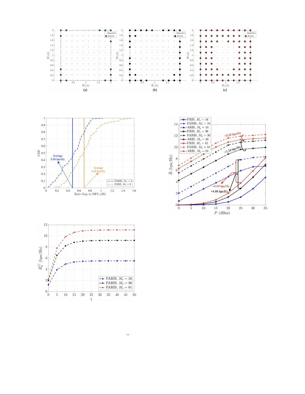
1 Fluid-Acti v e-RIS (F ARIS): A Ne w Smart-Radio P aradigm with Joint Port Selection and Acti v e Reflection Design Hong-Bae Jeon, Member , IEEE Abstract —In this paper , we introduce a new wireless paradigm termed fluid-active reconfigurable intelligent surface (F ARIS) that combines fluid-based port repositioning with per -element active amplification to enhance the performance of 6G netw orks. T o realistically characterize the hardware operation, we first dev elop a circuit-lev el abstraction of the F ARIS architectur e and establish a practical power consumption model that captures both the logical contr ol/switching power of candidate ports and the dir ect current (DC) bias power requir ed for active reflection. Based on this model, we establish the F ARIS signal model and f ormulate a corresponding ergodic-rate maximization problem that jointly optimizes the active amplification-reflection vector and the dis- crete selection of fluid-active elements under practical hardware constraints. The pr oblem is addressed via an alter nating opti- mization (A O) framework, which progressiv ely impro ves the rate. Complexity and conv ergence analyses that follow furnish deeper insight into the algorithmic operation and performance en- hancement. Numerical results confirm that the proposed F ARIS with the A O framework consistently outperforms con ventional baselines, delivering higher rates acr oss diverse en vir onments, often even when using fewer active elements or a smaller physical aperture. Index T erms —Fluid acti ve r econfigurable intelligent surface (F ARIS), ergodic rate, alternating optimization. I . I N T RO D U C T I O N R E C E N T L Y , reconfigurable intelligent surfaces (RISs) hav e emerged as a key technology for sixth-generation (6G) wireless networks, primarily due to their capability to pas- siv ely reconfigure the radio en vironment with minimal power consumption [1], [2]. An RIS typically comprises a large array of programmable, low-cost metasurf ace elements whose tun- able reflection characteristics enable fine-grained manipulation of electromagnetic wa ves [3]. By coordinating the phase shifts across these elements, RISs can intentionally steer , focus, or scatter incident signals, thereby improving coverage, link reliability , spectral ef ficiency , and ev en localization perfor- mance across diverse wireless scenarios [4]–[7]. Although RIS is recognized for its cost- and energy-efficienc y in boosting wireless cov erage and rate, its practical deployment remains challenging. One critical issue is that since con ventional RIS architectures rely solely on passiv e reflecting elements, it in- evitably suf fers from se vere multiplicati ve fading, as their end- to-end path loss (PL) is the product of the Tx-RIS and RIS- This work was supported by Hankuk University of F oreign Studies Research Fund of 2026. (Corr esponding Author: Hong-Bae J eon.) H.-B. Jeon is with the Department of Information Communications Engi- neering, Hankuk Uni versity of F oreign Studies, Y ong-in, 17035, K orea (e- mail: hongbae08@hufs.ac.kr). Rx channel losses. This fundamental limitation significantly degrades performance in practical deployments [8], [9]. T o address this fundamental physical bottleneck, recent research has introduced acti ve-RIS (ARIS) as a ne w archi- tecture for wireless systems [10], [11]. Unlike con ventional passiv e-RIS (PRIS) that merely reflects incident signals, ARIS incorporates reflection-type amplifiers into their elements, en- abling them to amplify the reflected signals. Although this requires additional power consumption, the resulting gain can effecti vely compensate for the se vere double-reflection path loss, making ARIS a promising solution to the “multiplicativ e fading” problem. Se veral studies ha ve further demonstrated the performance gains of ARIS in various wireless settings, including joint beamforming optimization with sub-connected architectures [12], signal-to-noise-ratio (SNR)-oriented analy- ses under identical po wer budget with PRIS [13], [14], and a v- erage sum-rate maximization [15] and power -minimizing [16] framew orks under partial channel-state-information (CSI) con- ditions, highlighting its potential to fundamentally enhance cov erage, reliability , and spectral ef ficiency . Another critical issue is that con ventional RIS architectures rely on a fixed and finitely quantized phase-control structure, which fundamentally limits their ability to realize the truly smart and highly adaptive wireless en vironment they were originally envisioned for [17]. As a result, practical RIS implementations often fall short of achieving en vironment- lev el reconfigurability , undermining the very motiv ation of deploying lo w-cost surfaces to offload comple xity from base stations (BSs) [18]. Furthermore, this fix ed structure is also un- fa vorable for achieving high degree-of-freedom (DoF) in RIS- aided channels [19], [20], as substantial DoF gains generally necessitate scaling up the RIS [21]–[23], ine vitably leading to increased training overhead and greater implementation complexity [24], [25]. Thus, the rigid structure of conv entional RIS not only limits its adaptability to smart environments but also fundamentally restricts scalable DoF enhancement, which additionally limits its ability to effecti vely mitigate the aforementioned multiplicativ e-fading effect. In this context, the concept of fluid antenna system (F AS) has emerged as a compelling solution [26], [27]. Unlike con ventional fixed-structure antennas, F AS offers shape- and position-reconfigurability enabled by fle xible materials and ar- chitectures [28], [29], thereby introducing additional physical- layer DoFs that can be exploited for performance enhance- ment [30]. Since the F AS is first introduced [26], se veral studies hav e been made to understand the various perfor- 2 mance limits of F AS [30]–[32], enable channel estimation schemes for F AS [33], [34], and apply with sev eral other applications including RIS [35], [36], integrated-sensing-and- communications (ISA C) [37], [38], and direction-of-arri val (DoA) estimations [39], [40]. T aken together, these studies establish F AS as a promising paradigm that surpasses con ven- tional antenna systems by unlocking higher spatial div ersity , and by of fering a versatile platform that can be seamlessly integrated into div erse 6G wireless functionalities. Inspired by the position-reconfigurability of F AS, recent work has extended this concept to RIS through the notion of fluid-RIS (FRIS) [41], [42], where the RIS hosts a mov able “fluid” elements capable of dynamically changing its posi- tion and applying optimized phase shifts [43]. By allowing a small number of mobile elements to traverse a larger physical aperture, FRIS ef fecti vely e xtracts spatial-domain DoFs without increasing the number of reflecting units [44], offering a fundamentally different path toward scalable DoF enhancement under practical hardware constraints [45]. While FRIS achieves meaningful performance gains through spatial- domain mobility , its reliance on passiv e reflection still lea ves substantial headroom for further enhancement. From this observ ation, we concei ve that the adv antages of spatial mobility and activ e reflection on RIS are not merely additiv e b ut fundamentally complementary . On the one hand, ARIS can compensate for sev ere cascaded path loss through signal amplification [11]; ho we ver , its amplification occurs ov er a fixed surface geometry , limiting the ability to con- centrate amplification on spatially fav orable locations. On the other hand, FRIS can adaptiv ely select advantageous spatial positions across a larger aperture [41], but passive reflection alone cannot suf ficiently overcome the inherent multiplicati ve- fading penalty [8]. Therefore, the key opportunity lies in a deeper integr ation where each selected element simultane- ously possesses spatial mobility and contr ollable amplification. In such a design, the surface can jointly optimize wher e the signal interaction occurs and how strongly the signal is reinforced, thereby creating a coupled spatial-amplitude design space that does not exist in conv entional FRIS or static ARIS architectures. Importantly , such an architecture should not be interpreted as a simple system-level stack- ing of FRIS and ARIS functionalities. Rather , it requires a fundamentally ne w metasurface structure in which each reflecting element operates as a fluidic activ e unit, capable of dynamically repositioning within its designated subregion while simultaneously applying controllable amplification and phase adjustment. Through this intrinsic integration, spatial selection and signal reinforcement become jointly controllable design v ariables, enabling the surface to adapt both the spatial distribution and strength of reflected energy . Motiv ated by this insight, we propose a fluid-active r econ- figurable intelligent surface (F ARIS) , a new RIS paradigm that tightly inte grates the spatial reconfigurability of FRIS with the signal amplification capability of ARIS. Unlike con ventional FRIS or static ARIS architectures, F ARIS equips each selected element with fluidic mobility together with active reflection functionality , allowing it to amplify and reflect incident signals while freely adjusting its position within the a vailable aperture. This dual capability enables F ARIS to simultaneously exploit position-adaptiv e spatial degrees of freedom and mitigate mul- tiplicativ e fading through controllable activ e gain. As a result, F ARIS provides a significantly stronger level of en vironment control compared with existing RIS architectures, offering a versatile platform for future 6G wireless networks. The main contributions are summarized as follo ws: 1) W e introduce a ne wly proposed F ARIS frame work for a do wnlink setting and develop a unified formulation for joint port selection and amplification-phase design. By explicitly modeling the spatial correlation among selected F ARIS ports and incorporating a practical ARIS reflection-power constraint, we cast an ergodic-rate max- imization problem that simultaneously optimizes the amplification-reflection vector and the discrete configu- ration of fluid-reconfigurable ports. In addition, based on a circuit-lev el modeling of the F ARIS architecture, we establish a practical power consumption model that captures both the control-circuit power and the direct current (DC) bias power of the acti ve reflection modules, which enables a realistic e valuation of the overall power consumption. 2) T o address the mixed-integer non-con vex nature of the problem, we de velop an alternating-optimization (A O) framew ork for design on F ARIS architecture. W ith the port configuration fixed, we employ sample average ap- proximation (SAA) together with a quadratic fractional transform to conv ert the objectiv e into a sequence of con vex conic subproblems in a lifted matrix variable. When the resulting solution is not rank-one, Gaussian randomization and magnitude projection are applied. W e additionally establish that this inner-loop procedure guarantees monotonic improvement of the SAA objec- tiv e and con ver gence to a stationary point. For discrete port selection under a cardinality constraint on the se- lectable F ARIS elements, given the current amplification- reflection vector , we propose a cardinality-constrained cross-entropy method (CEM) that draws Bernoulli se- lection samples and updates an independent Bernoulli distribution to fit the statistics of the high-rate elite subset. W e deriv e a closed-form CEM update, showing that the optimal selection probabilities are parametrized by a single Lagrange multiplier and that the resulting mapping admits a unique solution enforcing the cardinality budget. The smoothed update is prov en to monotonically increase the empirical log-likelihood, and yields a non-decreasing sequence of ergodic rates. 3) Building on these, we integrate the activ e-reflection de- sign and the port selection into a unified A O framework. W e prove that each outer iteration produces a non- decreasing sequence with finite limit by leveraging the monotonicity of the subproblems in A O frame work. W e conduct a detailed complexity analysis of each algorith- mic block, where the resulting expressions character - ize how the o verall computational cost scales, thereby confirming the polynomial-time implementability of the F ARIS with proposed A O framework. 3 Fig. 1. System model of F ARIS-aided wireless network. 4) Extensive simulations are performed over a wide range of system parameters, including transmit power , total number of F ARIS elements and candidates, and nor- malized aperture. The results show that the proposed F ARIS architecture with the A O framew ork exhibits fast conv ergence within a modest number of outer A O iterations and achieves near-optimal ergodic rate with only marginal loss compared to brute-force search (BFS), while drastically reducing computational burden. More- ov er , F ARIS consistently outperforms con ventional base- lines, achieving significantly higher rates ev en with fewer activ e elements or smaller apertures. In addition, the power consumption analysis demonstrates that F ARIS requires only a slightly higher power than ARIS due to the candidate port control, while providing substan- tially impro ved rate performance. Moreover , compared to the amplify-and-forward (AF) relay architecture, F ARIS av oids the excessi ve hardw are po wer consumption asso- ciated with complex architectures. As a result, F ARIS achiev es a more fav orable rate-po wer trade-of f among the considered architectures. T o the best of our knowledge, this is the first work to formalize F ARIS as a ne w RIS paradigm that intrinsically couples fluid port r econfigurability with active r eflection within a unified ar chitectur e. Supported by rigor ous algorithmic design, de- tailed complexity characterization, and extensive simulations, our results show that F ARIS is not mer ely a hybrid extension of existing RIS concepts, but a practically implementable and performance-enhancing paradigm that achie ves near-optimal operation while consistently outperforming con ventional FRIS and ARIS benchmarks. I I . S Y S T E M M O D E L As illustrated in Fig. 1, we examine a downlink wireless system assisted by F ARIS. A BS equipped with a single fixed-position antenna (FP A) communicates with a mobile user (MU), also equipped with a single FP A, through the F ARIS. The direct BS-MU link is assumed to be completely blocked by obstacles such as b uildings. The F ARIS consists of M = M x × M x reflectiv e elements arranged ov er a surface of size W x λ × W x λ , where λ denotes the carrier wa velength and W x represents the normalized aperture of the F ARIS relati ve to λ . The inter -element spacing is d = W x λ M x , resulting in a spatial Fig. 2. Schematic illustration of the F ARIS architecture with incorporating on-off control circuits and reflection-type amplifiers for the selected elements. correlation matrix J ≜ [ J ij ] ∈ R M × M modeled according to Jakes’ model. The spatial correlation between the i th and j th elements is given by [44], [45] J ij = j 0  2 π d ij λ  , (1) where j 0 ( · ) denotes the zero-order spherical Bessel function of the first kind, and d ij = d r (mo d( i, M x ) − mo d( j, M x )) 2 + j i M x k − j j M x k 2 is the distance between the i and j th elements. Following [42], [45] 1 and dif fering from [41], each F ARIS element can be viewed as a port of a fluid antenna structure. Each element operates in one of two states: “on” and “of f ”; In the “on” state, the element is connected to the activ e reflection branch and acti vely interacts with the incident electromagnetic wav e. Specifically , the impinging signal is processed through the controllable reflection circuitry , where its amplitude and phase can be adjusted according to the configured reflection coefficient. This enables the element to participate in the F ARIS reflection process and contrib ute to shaping and amplifiying the composite reflected wav e tow ard the desired direction. In contrast, in the “off ” state, the element is terminated by a matched load through the switching network. In this case, the incident electromagnetic energy is absorbed rather than re-radiated, ef fecti vely isolating the element from the reflection process and preventing an y modification of the impinging signal. Consequently , the element does not contribute to the reflected field and only incurs the baseline control-circuit power consumption. The schematic illustration of the F ARIS architecture is given in Fig. 2, which serves as the basis for the power consumption model dev eloped in the subsequent analysis. The BS-F ARIS link is assumed line-of-sight (LoS); ˜ h f ∈ C M , where as noted in [46], it occurs when the BS-FRIS distance is shorter than the advanced MIMO Rayleigh distance 1 Although the cited model is for FRIS, we adopt it here since F ARIS fol- lows the same hardware architecture, with the difference being the additional amplification module for each candidate. 4 (MIMO-ARD), represented as D RB ≜ λM . The F ARIS-MU link experiences Rician fading: h u = r K K + 1 ˜ h u + r 1 K + 1 ˆ h u ∈ C M × 1 , (2) where ˜ h u and ˆ h u ∼ C N (0 , I M ) are the deterministic LoS and the non-LoS (NLoS) component, respecti vely , where I M is an M × M identity matrix. Out of the total M candidate ports, only M o are selected. This selection process is represented as S T M o ≜ [ e i 1 · · · e i M o ] ∈ R M × M o ( ∀ i n ∈ { 1 , · · · , M } ) , (3) where e i denotes the i th canonical basis vector (i.e., the i th column of I M ). This construction implies that only the ports index ed by { i n } M o n =1 are acti ve on the F ARIS. T o ensure unique selection, all columns of S T M o must be mutually distinct, prev enting redundant port selection. The functionality of S M o -utilized F ARIS ports can be represented by a phase-shift Φ and amplifier matrix G : Φ = diag  e j ϕ 1 , · · · , e j ϕ M o  ( ∀ ϕ i ∈ [0 , 2 π )) , G = diag ( g 1 , · · · , g M o ) ( ∀ g i ∈ [0 , g max ]) . (4) The effecti ve operator A act of F ARIS is therefore A act ≜ J 1 2 S T M o diag( v ) S M o J 1 2 , (5) where v = [ v 1 · · · v M o ] T , v i = g i e j ϕ i ↔ diag ( v ) = ΦG (6) denotes the concatenated amplification ( { g i } ) and reflection ( { ϕ i } ) mechanism on F ARIS, where the magnitude and phase of v i correspond each, respectively . The BS transmits a unit-power symbol x with po wer P , and noise at the F ARIS and the MU are respectiv ely giv en by n r ∼ C N ( 0 , σ 2 r I M ) , z ∼ C N (0 , σ 2 0 ) . In summary , the signal s RIS radiated by F ARIS is s RIS = A act  p P L f ˜ h f x + n r  , (7) where L f is the PL of the BS-F ARIS link. The instantaneous radiated power P RIS at F ARIS is therefore P RIS = P L f ∥ A act ˜ h f ∥ 2 2 + σ 2 r tr ( A act A ∗ act ) , (8) which accounts for both the amplified incident signal compo- nent and the amplified thermal noise emitted by the F ARIS. In addition to P RIS , the F ARIS operation also incurs the per- element hardw are po wer consumption due to the selected fluid- activ e ports. Specifically , following the structure and circuit model in Fig. 2, the circuit po wer consumption of the F ARIS is composed of two components: i) P c : the logical control and switching po wer consumed by each candidate element, and ii) P DC : the DC bias power required for active reflection [14]. Since the logical control circuit exists for all M candidates while the acti ve reflection branch is given only for the selected M o F ARIS ports, the total F ARIS po wer consumption is modeled as P tot F ARIS ≜ M P c + M o P DC + ξ P RIS , 2 (9) 2 Note that for ARIS, M ← M o , and it returns to the con ventional ARIS power consumption model in [14]. where ξ ≜ 1 υ with υ ∈ (0 , 1] denoting the amplifier efficiency . Therefore, under the total F ARIS power budget P max ,t , the feasible reflection design must satisfy P tot F ARIS ≤ P max ,t , which is equiv alent to: P RIS ≤ υ ( P max ,t − M P c − M o P DC ) ≜ P max . (10) The receiv ed signal y at MU is y = p L u h ∗ u s RIS + z = p P L f L u h ∗ u A act ˜ h f x + p L u h ∗ u A act n r + z , (11) where L u denotes the PL of the F ARIS-MU link. From (11), the instantaneous signal-to-interference-noise-ratio (SINR) is γ = P L f L u | h ∗ u A act ˜ h f | 2 σ 2 0 + h ∗ u Bh u , (12) where B ≜ L u σ 2 r A act A ∗ act , and the er godic rate ¯ R is ¯ R ≜ E h u [log 2 (1 + γ )] . (13) Hence, the overall design problem of the F ARIS-enabled system can be formulated as max v , S M o ¯ R s.t. (10) , ∀| v i |≤ g max , S M o ∈ { 0 , 1 } M o × M . (14) Note that since diag( v ) = ΦG , we solve (14) and decompose { v i } into magnitude and phase, which corresponds to { g i } and { e j ϕ i } ( ↔ { ϕ i } ) , respectiv ely . I I I . P RO P O S E D AO F R A M E W O R K T o jointly optimize v ( ↔ ( Φ , G )) and S M o , we adopt an A O approach. A. Optimizing v ( ↔ ( Φ , G )) for F ixed S M o When S M o is fixed, define the lifted v ariable V as V ≜ vv ∗ ⪰ 0 (rank V = 1) . (15) W e approximate (13) via the SAA using S independent and identically distributed (i.i.d.) samples { h ( s ) } S s =1 of h u : ¯ R S ≜ 1 S S X s =1 log 2       1 + P L f L u | h ( s ) ∗ A act ˜ h f | 2 σ 2 0 + h ( s ) ∗ Bh ( s ) | {z } ≜ γ s       . (16) T o transform the problem with respect to V , we introduce the following theorem: Theorem 1. Define b ≜ S M o J 1 2 ˜ h f , u s ≜ S M o J 1 2 h ( s ) , K ≜ S M o JS T M o , (17) and a s ≜ u s ⊙ b , C s ≜ L u σ 2 r ( K ⊙ ( u s u ∗ s )) , (18) wher e b is the element-wise conjugate of b . Then the following hold: • γ s can be written as γ s = P L f L u v ∗ a s a ∗ s v σ 2 0 + v ∗ C s v = P L f L u tr( a s a ∗ s V ) σ 2 0 + tr( C s V ) . (19) 5 • P RIS satisfies P RIS = v ∗ ( P L f Q 1 + σ 2 r Q 2 ) v = tr( FV ) , (20) wher e F ≜ P L f Q 1 + σ 2 r Q 2 and Q 1 ≜ diag ( b ∗ ) K diag( b ) = K ⊙ ( bb T ) , Q 2 ≜ K ⊙ K . (21) Pr oof. See Appendix A. ■ Hence by Theorem 1, the acti ve reflection design subprob- lem becomes max V 1 S S X s =1 log 2  1 + P L f L u tr( a s a ∗ s V ) σ 2 0 + tr( C s V )  s.t. tr( FV ) ≤ P max , V ii ≤ g 2 max ( i = 1 , · · · , M o ) , rank V = 1 , V ⪰ 0 , (22) where V ii is the ii th component of V . Problem (22) is still not con vex due to the fractional objectiv e and the rank-1 constraint. T o handle the noncon ve x fractional structure, we will drop the rank constraint and apply a fractional/quadratic transform to obtain a sequence of con vex conic subproblems in V , followed by Gaussian randomization [47] and magnitude projection if necessary . W e first apply the quadratic transform, also known as the fractional programming technique, to (22). For each s , introduce an auxiliary variable y s ≥ 0 and use the following transformation for A ≥ 0 and B > 0 [48]: A B = max y ≥ 0 (2 y √ A − y 2 B ) , (23) where the unique maximizer is gi ven by y ⋆ = √ A B . Equa- tion (23) con verts a ratio into a concav e quadratic form with respect to y ≥ 0 and yields a closed-form update for y gi ven the other variables, enabling alternating optimization for sum- of-log-fraction objectiv es. Applying the result to (19), (16) is equiv alently lower-bounded as ¯ R S ≥ 1 S S X s =1 log 2 (1 + ξ s ) , ξ s ≜ P L f L u  2 y s p tr( a s a ∗ s V ) − y 2 s ( σ 2 0 + tr( C s V ))  ( ≥ 0) , (24) where the maximum ξ s = γ s holds by substituting y s = √ tr( a s a ∗ s V ) σ 2 0 +tr( C s V ) . W e will therefore maximize 1 S P S s =1 log 2 (1 + ξ s ) as the lo wer-bound of objecti ve in (22), which is constructed by the following procedure: 1) Update of V ( ↔ v ) for fixed { y s } : Since p tr( a s a ∗ s V ) in (24) is noncon ve x with respect to V , by introducing the slack variables { w s ≥ 0 } S s =1 , p tr( a s a ∗ s V ) is handled by w s subject to the second-order cone (SOC) Q r [49]:  w s , p tr( a s a ∗ s V )  ∈ Q r ↔ w s ≤ p tr( a s a ∗ s V ) , (25) which is equi valent to stating that w s forms the hypograph of p tr( a s a ∗ s V ) . Hence, for fixed { y s } , the transformed subproblem becomes max V , { w s ,ξ s } 1 S S X s =1 log 2 (1 + ξ s ) s.t. ξ s ≤ P L f L u  2 y s w s − y 2 s ( σ 2 0 + tr( C s V ))  ,  w s , p tr( a s a ∗ s V )  ∈ Q r , w s ≥ 0 , ξ s ≥ 0 , V ⪰ 0 , tr( FV ) ≤ P max , V ii ≤ g 2 max . ( i = 1 , · · · , M o , s = 1 , · · · , S ) . (26) Problem (26) is a con ve x conic optimization problem with linear matrix inequality (LMI) and SOC constraints. Upon solving it, if the optimal V 0 is rank-one, the corresponding v 0 is directly obtained as its principal eigenv ector satisfying V 0 = v 0 v ∗ 0 . Otherwise, v 0 is extracted via Gaussian random- ization, starting by computing the Cholesky factorization of V 0 : V 0 = LL ∗ [50], where L is a lower -triangular matrix. W e then generate N rand independent Gaussian realizations: v n = Lz n ( n = 1 , · · · , N rand ) , (27) where { z n ∼ C N ( 0 , I M o ) } are i.i.d. standard circularly symmetric complex Gaussian random vectors. For each v n , we first enforce feasibility with respect to the hardware constraints. Specifically , we apply an element-wise magnitude projection to satisfy { V ii ≤ g 2 max } in (26), [ v n ] i ← min { g max , | [ v n ] i |} e j  [ v n ] i ( i = 1 , · · · , M o ) , (28) followed by a global power scaling v n ← α n v n , α n ≜ min ( 1 , s P max v ∗ n Fv n ) , (29) which guarantees v ∗ n Fv n ≤ P max in (26). Let v feas n denote the resulting feasible v ector and define the corresponding rank- one matrix V n ≜ v feas n v feas ∗ n . For each V n , we ev aluate the objecti ve in (22), denoted by ˜ R n , then select the best randomized candidate as n ⋆ = arg max n ∈{ 1 , ··· ,N rand } ˜ R n , (30) which corresponds to v feas n ⋆ . 2) Update of y s for fixed V : For fixed V , each y s admits the closed-form update y ⋆ s = w s σ 2 0 + tr( C s V ) ( s = 1 , · · · , S ) . (31) By alternately updating V from (26) and { y s } from (31), the objectiv e is guaranteed to be non-decreasing until con ver gence, which will be shown later . The o verall procedure is gi ven by Algorithm 1. Remark 1 . In Algorithm 1, we initialize v [0] ( ↔ V [0] ) by drawing i.i.d. θ i ∼ U [0 , 2 π ) , set ¯ v = g max [ e j θ 1 · · · e j θ M o ] T , and scale ¯ v → v [0] so that v [0] ∗ Fv [0] ≤ P max . This guarantees feasibility of (10) and ∀| v [0] i |≤ g max . Thereafter, we set y [0] s = √ tr( a s a ∗ s V [0] ) σ 2 0 +tr( C s V [0] ) ( ∀ s ) . 6 Algorithm 1 A O Framework of v and { y s } for Fixed S M o 1: Input: { h ( s ) } S s =1 , ϵ v , S M o 2: Initialize: v [0] ( ↔ V [0] ) satisfying (10) and ∀| v [0] i | < g max , { y [0] s } , t ← 0 3: Evaluate ¯ R [0] S by (16) 4: repeat 5: Solve (26) to obtain V [ t +1] 6: if rank V [ t +1] > 1 then 7: Extract v [ t +1] via Gaussian randomization 8: else 9: v [ t +1] ← principal eigenv ector of V [ t +1] 10: end if 11: for s = 1 , · · · , S do 12: Update y [ t +1] s via (31) using V [ t +1] 13: end for 14: Evaluate ¯ R [ t +1] S by (16) 15: t ← t + 1 16: until | ¯ R [ t ] S − ¯ R [ t − 1] S | < ϵ v 17: v † ← v [ t ] ( ↔ V † ← V [ t ] ) 18: Output: v † ( ↔ V † ) 3) Monotonicity and Con ver gence Analysis of Algorithm 1: T o ensure that Algorithm 1 produces stable performance improv ements, it is essential to verify that each iteration does not degrade ¯ R S . The follo wing theorem establishes this monotonicity property . Theorem 2. In Algorithm 1, { ¯ R [ t ] S } monotonically non- decr eases. Pr oof. See Appendix B. ■ Furthermore, since the feasible set of V is compact due to the constraints tr( FV ) ≤ P max and V ii ≤ g 2 max ( i = 1 , · · · , M o ) in (22), { ¯ R [ t ] S } is bounded above. Therefore, { ¯ R [ t ] S } t ≥ 0 con verges to a finite limit. B. Optimizing S M o for fixed v T o stochastically determine the activ e ports for giv en v , each port i is assigned an selection probability p i ∈ [0 , 1] , forming the probability vector p = [ p 1 · · · p M ] T . Let ζ = [ ζ 1 · · · ζ M ] T ∈ { 0 , 1 } M denote a random binary port-selection vector sampled as ζ ∼ Bernoulli( p ) , P ( ζ ; p ) = M Y i =1 p ζ i i (1 − p i ) 1 − ζ i . (32) W e propose to utilize an M o -constrained CEM that fits an independent Bernoulli law ζ ∼ Bernoulli( p ) to the elite set of high-performing port subsets while exactly enforcing the expected-cardinality budget P M i =1 p i = M o [43], [45], [51]. 1) Ideal T arget Distribution: Let Z ⊆ { 0 , 1 } M denote the set of all feasible binary port-selection vectors, and let ¯ R S ( ζ ) be the objective in (16) corresponding to ζ ∈ Z . Define the elite threshold γ ρ as the (1 − ρ ) -quantile of ¯ R S ( ζ ) under the current sampling distribution, so that a fraction ρ of samples satisfy ¯ R S ( ζ ) ≥ γ ρ . The ideal target distribution P † ( ζ ) that perfectly concentrates on the elite set is then P † ( ζ ) ∝ ( 1 ( ¯ R S ( ζ ) ≥ γ ρ ) 0 ( otherwise ) . (33) Intuitiv ely , P † assigns nonzero probability only to high- performing (elite) selection patterns. The CEM seeks P ( ζ ; p ) that approximates P † as closely as possible. F ormally , this is achie ved by minimizing the Kullback-Leibler (KL) div ergence: p new ≜ arg min p D KL ( P † ∥ P ( · ; p )) = arg max p E P † [ log P ( ζ ; p )] . (34) Since P † is unknown, we approximate the expectation in (34) using the empirical distrib ution of the elite samples: E P † [ log P ( ζ ; p )] ≈ 1 N e X n ∈E log P ( ζ n ; p ) , (35) where we dra w N mc i.i.d. samples { ζ n } N mc n =1 from Bernoulli( p ) and ev aluate { ¯ R S ( ζ ) } N mc n =1 . Let E be the elite index set of the top- ρ fraction, with size of N e = ⌈ ρN mc ⌉ by definition. Maximizing (35) yields p new = arg max p ∈ [0 , 1] M 1 N e X n ∈E log P ( ζ n ; p ) . (36) which is exactly the empirical log-likelihood maximization used in the CEM update rule. 2) Applying to M o -constrained CEM with Iterations: W e now modify the CEM with the aforementioned cardinality b ud- get. Herein at iteration t , draw N mc i.i.d. samples { ζ [ t ] n } N mc n =1 from Bernoulli( p [ t ] ) and ev aluate { ¯ R S ( ζ [ t ] n ) } N mc n =1 . Let E [ t ] be the elite index set of the top- ρ fraction, with size of N e = ⌈ ρN mc ⌉ by definition. Then we can define the elite empirical average per coordinate i : µ [ t ] i ≜ 1 N e X n ∈E [ t ] ζ [ t ] n,i , (37) where ζ [ t ] n,i is the i th component of ζ [ t ] n ( i = 1 , · · · , M ) . By substituting into (36), it becomes max p Φ( p ) ≜ M X i =1  µ [ t ] i log p i + (1 − µ [ t ] i ) log(1 − p i )  s.t. M X i =1 p i = M o , p ∈ (0 , 1) M . (38) Problem (38) is strictly concav e with an affine constraint, hence admits a unique global maximizer, as characterized in the following theorem. Theorem 3. Let ν ∈ R be the Lagrang e multiplier . The unique maximizer of (38) satisfies, for each i , ν p 2 i − ( ν + 1) p i + µ [ t ] i | {z } ≜ f ( p i ,ν ) = 0 , (39) 7 Algorithm 2 CEM-Based Selection of S M o for Fixed v 1: Input: M o , ρ, N mc , ω , ϵ c , v 2: Initialize: p [0] ∈ (0 , 1) M with P i p [0] i = M o (e.g., uniform distribution), t ← 0 3: repeat 4: Draw ζ [ t ] n ∼ Bernoulli( p [ t ] ) ( n = 1 , · · · , N mc ) 5: Compute { ¯ R S ( ζ [ t ] n ) } N mc n =1 using v 6: E [ t ] ← indices of top- ρ samples by ¯ R S 7: Compute { µ [ t ] i } M i =1 by (37) 8: Find the unique ν † from (40) 9: Update p [ t +1] by (41) 10: t ← t + 1 11: until || p [ t +1] − p [ t ] || < ϵ c 12: b I ← top - M o ( p [ t ] ) and form S † M o by b I 13: Output: S † M o whose solution in (0 , 1) is p i ( ν ) =      µ [ t ] i ( ν = 0) ( ν + 1) − q ( ν + 1) 2 − 4 ν µ [ t ] i 2 ν ( ν  = 0) . (40) Mor eover , the mapping ν 7→ P M i =1 p i ( ν ) is strictly decreasing and continuous on its domain. Hence there exists a unique ν † such that P i p i ( ν † ) = M o . Pr oof. See Appendix C. ■ Giv en ν † , let p CE ≜ p ( ν † ) the exact maximizer of CEM in (38). A standard smoothed update is then p [ t +1] = (1 − ω ) p [ t ] + ω p CE ( ω ∈ (0 , 1)) , (41) which preserves the expected “ M o -sum” b udget e xactly since P i p [ t ] i = P i p i ( ν † ) = M o and by linearity in (41), and improv es Φ by follo wing theorem. Theorem 4. p CE = p ( ν † ) strictly increases Φ unless p [ t ] alr eady solves (38) . Mor eover , for any ω ∈ (0 , 1] , the smoothed update (41) yields Φ( p [ t +1] ) ≥ Φ( p [ t ] ) . Pr oof. Strict conca vity and uniqueness of the maximizer imply Φ( p CE ) > Φ( p [ t ] ) unless optimality holds at p [ t ] . For the smoothed step, p [ t +1] = (1 − ω ) p [ t ] + ω p CE remains feasible due to the strict concavity , and the concavity of Φ giv es Φ( p [ t +1] ) ≥ (1 − ω )Φ( p [ t ] ) + ω Φ( p CE ) ≥ Φ( p [ t ] ) , and the theorem follows. ■ The overall procedure is summarized in Algorithm 2, whose monotonicity and con vergence is guaranteed by theories of CEM in [51]. After verifying that the proposed algorithm concentrates p [ t ] to P † , we finally choose b I by selecting the top- M o indices of p [ t ] , and form the optimal S † M o . C. Overall Pr ocedur e The two subproblems in Section III-A and III-B are alter - nately solved until conv er gence: · · · → S ( t ) M o → V ( t +1) → S ( t +1) M o → · · · , (42) Algorithm 3 Overall A O Framework 1: Initialize: v (0) , S (0) M o , t ← 0 2: Compute ¯ R (0) S by (16) 3: repeat 4: Giv en S ( t ) M o , run Algorithm 1 to obtain v ( t +1) 5: Giv en v ( t +1) , run Algorithm 2 to obtain S ( t +1) M o . 6: ¯ R ( t +1) S ← 1 S P S s =1 log 2 (1 + γ s ( v ( t +1) , S ( t +1) M o )) 7: t ← t + 1 8: until | ¯ R ( t +1) S − ¯ R ( t ) S | < ϵ out 9: Output: v ⋆ ← v ( t ) , S ⋆ M o ← S ( t ) M o , ¯ R ⋆ S ← ¯ R ( t ) S where the o verall procedure is giv en in Algorithm 3. Note that v (0) is initialized according to Remark 1, while S (0) M o is generated by randomly selecting M o activ e ports from the M av ailable candidates. This proposed A O frame work ef fectively decouples the continuous reflection design and the discrete port-selection, while ensuring monotonic impro vement of the ov erall objectiv e. D. Overall Con ver gence of Algorithm 3 W e now combine the abov e results to discuss the conv er - gence of the full A O procedure in Algorithm 3, Let ¯ R ( t ) S denote the SAA objective value in (16) ev aluated at ( v ( t ) , S ( t ) M o ) in Algorithm 3. Then, for each outer iteration t : • Given S ( t ) M o , Algorithm 1 produces v ( t +1) such that ¯ R S ( v ( t +1) , S ( t ) M o ) ≥ ¯ R S ( v ( t ) , S ( t ) M o ) , (43) due to the monotonicity property by Theorem 2 • Given v ( t +1) and sufficiently large N mc , Algorithm 2 yields S ( t +1) M o which guarantees [51] ¯ R S ( v ( t +1) , S ( t +1) M o ) ≥ ¯ R S ( v ( t +1) , S ( t ) M o ) . (44) Therefore, the outer A O iterates generate a (deterministically or in expectation) non-decreasing sequence ¯ R (0) S ≤ ¯ R (1) S ≤ · · · ≤ ¯ R ( t ) S ≤ · · · (45) which is bounded above by the maximum achiev able rate under the gi ven power and hardware constraints. Consequently , { ¯ R ( t ) S } conv er ges to a finite ¯ R ⋆ S with its limit point ( v ⋆ , S ⋆ M o ) . I V . C O M P L E X I T Y A NA LY S I S W e characterize the computational complexity of the pro- posed A O framew ork for F ARIS by each step on Algorithm 3. A. Complexity of SAA-Based Rate Evaluation For fixed ( v , S M o ) , the SAA objectiv e ¯ R S in (16) requires to compute { γ s } in (19), which is dominated by each denom- inator term v ∗ C s v with O ( M 2 o ) operations. Hence, the rate ev aluation yields the complexity of O ( S M 2 o ) . 8 B. Complexity of Algorithm 1 1) V ariable and Constraint Dimensions: In order to charac- terize the computational complexity of the subproblem in (26), we explicitly define the dimensions of the optimization v ari- ables and the associated constraints: n v ar = M 2 o + 2 S, n cone = M 2 o + 3 S, n lin = M o + 1 + 3 S, (46) where n v ar is the number of decision variables, n cone is the total conic dimension, and n lin is the number of linear inequality constraints. 2) Interior-P oint Complexity of Solving (26) : A generic primal-dual interior -point step for mixed LMI/SOC problems incurs complexity of [49] O  n 3 v ar + n 2 v ar n cone + n v ar n 2 cone + n 2 v ar n lin  . (47) Substituting (46) to (47), the computational complexity Cost sub of solving (26) with K IP steps is given by O  K IP  ( M 2 o + 2 S ) 3 + ( M 2 o + 2 S ) 2 ( M 2 o + 3 S ) + ( M 2 o + 2 S )( M 2 o + 3 S ) 2 + ( M 2 o + 2 S ) 2 ( M o + 1 + 3 S )  = O ( K IP ( M 2 o + S ) 3 ) . (48) 3) Gaussian Randomization: The Cholesky factorization of V 0 requires O ( M 3 o ) flops and is performed once [50]. F or each z n ∼ C N ( 0 , I M o ) , v n = Lz n is generated with complexity O ( M 2 o ) . Each v n is then projected onto the feasible set by (28) and (29), dominated by latter one with O ( M 2 o ) operations. For each feasible v n , we form V n = v n v ∗ n and ev aluate ˜ R n by computing { tr( C s V n ) , tr( a s a ∗ s V n ) } S s =1 in the objectiv e of (22), which requires O ( S M 2 o ) operations; hence, the cost per randomized candidate is O ( S M 2 o ) . Consequently , the ov erall computational complexity is O  M 3 o + N rand S M 2 o  . (49) 4) Auxiliary Update: Updating y s via (31) requires tr( C s V ) with complexity of O ( S M 2 o ) . Hence, the total complexity of Algorithm 1 with T v itera- tions is given by Cost v -update = O  T v ( K IP ( M 2 o + S ) 3 + N rand ( S M 2 o + K ′ IP S 3 ))  . (50) C. Complexity of Algorithm 2 1) Sampling and Rate Evaluation: At iteration t of Al- gorithm 2, we draw N mc i.i.d. { ζ [ t ] n } . Since generating one such vector requires M independent Bernoulli trials, the total sampling complexity is O ( N mc M ) . For each ζ [ t ] n , we e v aluate { ¯ R S ( ζ [ t ] n ) } N mc n =1 . Thus, by the result in Section IV -A, the total complexity of ev aluating all N mc samples is O ( N mc S M 2 o ) . Fig. 3. Simulation setup of the F ARIS-aided system. 2) Elite Selection and Statistics: Thereafter , we select the top- ρ fraction of samples as E [ t ] . Sorting the N mc fit- ness values requires O ( N mc log N mc ) , which is optimal for comparison-based sorting. Once E [ t ] of size ⌈ ρN mc ⌉ is de- termined, µ [ t ] i in (37) must be computed. Each µ [ t ] i requires summing the i th entries of N e binary vectors of length M . Therefore, the overall complexity of computing all M components of µ [ t ] is O ( ρN mc M ) . 3) Solving for ν † : Each ev aluation of g ( ν ) costs O ( M ) , and bisection with L ν steps giv es O ( L ν M ) . Hence, the total complexity of Algorithm 2 with T CEM iterations is given by Cost S -update = O  T CEM ( N mc S M 2 o + N mc M + N mc log N mc + L ν M )  . (51) D. Overall A O Complexity Combining the results, we get the total complexity of the proposed A O frame work with T AO iterations as Cost total = O  T AO  Cost v -update + Cost S -update + S M 2 o  . (52) V . S I M U L A T I O N R E S U L T S In the simulations, we assess the effecti veness of the pro- posed A O framew orks for maximizing ¯ R through Monte-Carlo ev aluations. The F ARIS setup, as shown in Fig. 3, considers a deployment of the BS, F ARIS, and MU, with distances l f = 3 m and l u = 15 m . Since l f = 3 m is smaller than D RB = 6 m , the LoS condition for ˜ h f is satisfied [46]. The channels between the ARIS and MU are modeled as flat Rician f ading channels, with a path-loss e xponent of 2.2 and K = 1 [52], [53], and the detailed simulation parameters are listed in T able I. Each Monte-Carlo point is computed by av eraging o ver 10 3 independent realizations of signal trans- mission and reception. For comparison, we also include the performance of (i) a con ventional FRIS (passi ve) architecture with the same number of M o FRIS elements selected from M candidates with the particle-swarm-optimization (PSO)-based 9 T ABLE I S I MU L A T IO N P A RA M E T ER S Parameter V alue Number of F ARIS/FRIS elements M (unless referred) 100 ( 10 × 10 ) Maximum amplification gain g max 40 [dB] [14] Hardware power consumption ( P c , P DC ) (-10, -5) [dBm] [14] T otal power budget of F ARIS P max ,t 25 [dBm] [14] T ransmit power P (unless referred) 15 [dBm] Noise at F ARIS and MU ( σ 2 r , σ 2 0 ) -90 [dBm] (same) Normalized F ARIS/FRIS aperture W x (unless referred) 2 Parameters in CEM ( N mc , ρ, ω ) (5 N , 0 . 1 , 0 . 7) [51] approach in [41], and (ii) an ARIS architecture with same M o elements with sequential con ve x approximation (SCA)-based optimization in [14]. W e additionally compare our results with a BFS baseline that e xhausti vely ev aluates every possible port-phase configuration of the FRIS, assuming a b = 2 -bit discrete phase quantization and one-dimensional search over [0 , g max ] [45]. Fig. 4 depicts the preset position candidates for the F ARIS when employing M o = 16 , 36 and 81 fluid elements, which show the inherent fle xibility of the F ARIS architecture. For each case, the most advantageous S ⋆ M o is determined by CEM- based Algorithm 2. The resulting element selections show a clear tendency to fa vor ports located near the boundary of the array rather than those concentrated around the center . This phenomenon can be interpreted from the perspecti ve of the ef fecti ve aperture and spatial div ersity provided by F ARIS. In particular, elements positioned farther from the array centroid typically experience larger angular separation and more div erse propagation geometries. As a result, they tend to exhibit lower spatial correlation and contribute more effecti vely to enlarging the achiev able di versity and DoF through the optimized configuration of G . Fig. 5 depicts the cumulati ve distribution function (CDF) of the ergodic-rate gap, together with that of the BFS benchmark, for M = 16 and M o ∈ { 4 , 9 } . Notably , the F ARIS equipped with the proposed A O framework achie ves near-optimal per - formance, closely tracking the exhausti ve BFS curve despite the dramatic reduction in computational burden. The a verage gap remains as small as 0.48 and 0.69 bps/Hz for M o = 4 and 9 , respecti vely , a practically negligible loss considering that BFS requires ev aluating the entire discrete port-phase space and optimal amplification control, whereas our method con verges rapidly with orders-of-magnitude lower complexity . This highlights the ef ficiency and scalability of the proposed A O frame work, e ven under stringent configuration constraints. Fig. 6 illustrates the conv ergence behavior of ¯ R ( t ) S with the proposed A O framework for dif ferent values of M o . The proposed algorithm shows a monotonic increase in the objectiv e and typically con verges within 15-20 iterations. The con vergence speed is acceptable even though F ARIS has more control variables (amplification + phase + port selection) than the FRIS baseline, demonstrating its practicality for real- time implementation in F ARIS. Furthermore, as M o increases, con vergence becomes slightly slower due to the enlarged search space and stronger spatial correlation, which lessen the marginal gain achiev ed at each iteration [54]. Fig. 7 presents ¯ R versus P for F ARIS and con ventional FRIS/ARIS under M o = 16 , 36 and 81 . As P increases, F ARIS with the proposed A O framework and ARIS initially exhibit a steeper rate gro wth; ho we ver , after certain threshold of P , the hardw are constraint (10) in (14) becomes active, causing both curves to transition into a more moderate scaling with respect to P [14]. Consequently , the optimization gain of F ARIS ov er ARIS also diminishes slightly in this high- power re gime, as the ARIS amplification is limited by the same hardware bound. Nev ertheless, F ARIS still preserves a substantial rate margin over FRIS/ARIS, ev en with small M o , as its fluid positioning and activ e amplification enable more effecti ve e xploitation of the aperture and yield sustained rate gains ov er the counterparts; at P = 25 dBm, the F ARIS with M o = 36 and 81 yields 0.36 and 0.73 bps/Hz higher rate compared to ARIS architecture. Furthermore, with same P = 25 dBm, the F ARIS configuration with M o = 16 attains an a verage rate of approximately 7.97 bps/Hz, whereas the FRIS setup, despite employing a much larger aperture, achiev es no more than 3.93 bps/Hz at M o = 81 , meaning that F ARIS pro vides a 4.04 bps/Hz higher rate. This performance gap widens further for M o = 36 , making the rate of F ARIS 4.98 bps/Hz higher . Moreov er , increasing M o improv es ¯ R for ev ery architecture; howe ver , the marginal gain decreases for larger M o with fix ed M , reflecting a saturation due to dense spatial sampling shown in Fig. 4. Fig. 8 depicts the v ariation of ¯ R with respect to M (or equiv alently M x ) in the F ARIS and con ventional FRIS/ARIS configuration. For any fixed M, F ARIS equipped with the proposed A O framework consistently achie ves a higher rate than FRIS/ARIS, e ven with less M o ; when M x = 16 , the proposed F ARIS configuration with M o = 16 provides an additional 3.53 bps/Hz over FRIS with M o = 81 , which increases to 4.20 bps/Hz when M o = 36 , and the gain over ARIS, whose fixed architecture yields a nearly flat rate profile due to the absence of extra DoFs or adaptiv e optimization, becomes readily apparent in the figure. This again highlights the substantial rate gain enabled by both fluid repositioning and active amplification. As M increases, both F ARIS/FRIS architectures benefit from the denser aperture, which enhances spatial sampling and increases the likelihood of selecting more fa vorable element positions. Despite this common scaling benefit, F ARIS maintains a clear performance margin over FRIS, as its fluid port placement together with acti ve am- plification enables more effecti ve utilization of the expanded aperture, thereby pro viding rate enhancements unattainable by the purely passive counterpart. Fig. 9 illustrates ¯ R as a function of W x for both F ARIS and con ventional FRIS. In the initial growth region, all schemes, including the proposed A O-enabled F ARIS and the con ven- tional FRIS, exhibit a sharp increase in ¯ R due to the rapid reduction in spatial correlation and the improved ability to select fav orable port positions as the aperture expands. This effect is also considerably pronounced for F ARIS, similar to the previous observation, so that ev en a F ARIS design with a smaller element count (e.g., M o = 16 ) can surpass the rate of a lar ger-aperture FRIS configuration (e.g., M o = 36 , 81 ). 10 Fig. 4. Illustration of examples of the optimized positions when the F ARIS has (a) M o = 16 (b) M o = 36 (c) M o = 81 fluid activ e elements. Fig. 5. CDF of ergodic rate gap between BFS and proposed A O frameworks for different M o with M = 16 . Fig. 6. Conv ergence performance of ¯ R ( t ) S by the proposed A O framework for different M o . As W x ⪆ 5 , which corresponds to spacing of λ 2 , the rate improv ement begins to saturate since the additional aperture provides only mar ginal decorrelation benefits [31]. Notably , in this re gion, F ARIS exploits the enlar ged aperture far more effecti vely than FRIS, thanks to its jointly optimized fluid positioning and activ e amplification. Therein with W x = 6 , the rate difference between F ARIS with M o = 16 and FRIS Fig. 7. Achievable rate ¯ R versus Tx power P for different M o F ARIS/FRIS elements. when M o = 81 is 3.27 bps/Hz, which further widens to 3.73 bps/Hz when the number of active FRIS elements is reduced to M o = 36 . Although all schemes ev entually show saturation after W x ⪆ 5 , F ARIS maintains a consistently lar ger gain throughout the entire range of W x . Fig. 10 illustrates the total power consumption versus M o for the proposed F ARIS architecture, con ventional ARIS, and AF relay . Herein, the hardware power consumption of the M o - element AF relay is modeled as [55]. P hard , AF = M o ( P DA C + P mix + P filt ) + P syn , (53) where P DA C , P mix , P filt , and P syn denote the power con- sumption of the digital-to-analog con verter (D A C), mixer , filter , and frequency synthesizer , respectiv ely . According to the practical parameters reported in [55], the combined circuit power P DA C + P mix + P filt is approximately 18 . 2 dBm, while P syn = 17 dBm. This hardware power is then combined with the communication-related power for AF relays [56], [57]. As shown in the figure, compared with F ARIS, the ARIS architecture consistently e xhibits lo wer total power consump- tion across the considered range of M o . This is mainly due to the structural difference between the two architectures. In 11 Fig. 8. Achievable rate ¯ R versus the number of total elements M ( M x × M x ) for different M o F ARIS/FRIS elements. Fig. 9. Achievable rate ¯ R versus normalized aperture W x for dif ferent M o F ARIS/FRIS elements. ARIS, the acti ve elements are directly deployed at the selected M o positions, resulting in a smaller hardware power term M o ( P c + P DC ) as well as a reduced reflected signal power P RIS . In contrast, F ARIS maintains a lar ger candidate pool with M ports, which introduces an additional control-circuit power M P c in (9). Nev ertheless, the power consumption of F ARIS remains significantly lower than that of the AF relay . This is because unlike the AF relay nodes that operate as independent transceiv ers with dedicated radio-frequenc y (RF) chains and signal forwarding operations [56], [57], whose hardware po wer in (53) introduces substantially higher to- tal power , F ARIS remains a metasurface-based structure in Fig. 2 that directly manipulates the impinging electromagnetic wa ve ov er a distributed aperture. Therefore, F ARIS provides a fa vorable intermediate design that achie ves notable rate improv ements ov er ARIS while av oiding the excessi ve power ov erhead associated with AF relay architectures. V I . C O N C L U S I O N In this paper , we proposed the F ARIS concept, a novel fluid- activ e-RIS architecture that jointly exploits fluid port repo- Fig. 10. T otal power consumption versus M o for the proposed F ARIS and con ventional ARIS and AF relay architectures. sitioning and per-port amplification to substantially enhance the performance of RIS-aided wireless networks. T o capture the practical hardware behavior , we developed a circuit- aware modeling frame work and established a correlated F ARIS signal model based on Jakes’ spatial correlation. Under a realistic reflection-po wer constraint, we formulated an ergodic- rate maximization problem that jointly optimizes the activ e amplification-reflection coef ficients and the discrete selection of fluid-acti ve ports. T o solve the resulting mixed-integer non- con vex problem, we developed an A O-based framework that efficiently alternates between active-reflection optimization and CEM-based port selection, achieving near-optimal per- formance with significantly reduced computational complex- ity . Numerical results demonstrate that the proposed F ARIS architecture consistently outperforms con ventional baselines, achieving higher ergodic rates ev en with fewer active ele- ments than the benchmark schemes, thereby highlighting the efficienc y of the proposed fluid-activ e design. These results highlight that the syner gy between fluid reconfigurability and activ e amplification introduces a powerful additional spatial DoF , enabling more ef ficient channel shaping and positioning F ARIS as a promising architectural paradigm for 6G. A P P E N D I X A P RO O F O F T H E O R E M 1 W e first pro ve (19). From (5) and (17), h ( s ) ∗ A act ˜ h f = u ∗ s diag( v ) b , (54) and the square of magnitude becomes | h ( s ) ∗ A act ˜ h f | 2 = v ∗ a s a ∗ s v = | a ∗ s v | 2 , (55) which is the numerator of γ s in (16). Thereafter, the ARIS- induced noise term satisfies h ( s ) ∗ A act A ∗ act h ( s ) = u ∗ s diag( v ) K diag( v ∗ ) u s = v ∗ ( K ⊙ ( u s u ∗ s )) v , (56) Thus by (55) and (56), the denominator of γ s in (16) is σ 2 0 + v ∗ C s v ( C s ≜ L u σ 2 r ( K ⊙ ( u s u ∗ s ))) , (57) 12 and using V = vv ∗ and tr( Xvv ∗ ) = v ∗ Xv , we obtain (19). W e now prove (20). Again by using (5) and (17), ∥ A act ˜ h f ∥ 2 2 = v ∗ Q 1 v , Q 1 ≜ diag ( b ∗ ) K diag( b ) = K ⊙ ( bb T ) . (58) Similarly , tr ( A act A ∗ act ) = tr(diag( v ∗ ) K diag( v ) K ) = v ∗ Q 2 v ( Q 2 ≜ K ⊙ K ) . (59) Therefore, by defining F ≜ P L f Q 1 + σ 2 r Q 2 , P RIS becomes P RIS = v ∗ Fv = tr( FV ) , (60) and the theorem follo ws. ■ A P P E N D I X B P RO O F O F T H E O R E M 2 At iteration t of Algorithm 1, we assume that ( V [ t ] , { y [ t ] s } S s =1 ) has been obtained. By construction of the update rule in (31), the equality holds in the quadratic- transform lower -bound in (24) at V [ t ] , i.e., ¯ R [ t ] S = 1 S S X s =1 log 2 (1 + ξ [ t ] s ) , (61) where ξ [ t ] s denotes ξ s ev aluated at ( V [ t ] , { y [ t ] s } ) . Fixing { y [ t ] s } , we solve (26) to obtain V [ t +1] . Since V [ t +1] maximizes the lower -bound in (24) for fixed { y [ t ] s } , it holds that 1 S S X s =1 log 2 (1 + ¯ ξ [ t +1] s ) ≥ 1 S S X s =1 log 2 (1 + ξ [ t ] s ) , (62) where ¯ ξ [ t +1] s denotes ξ s ev aluated at ( V [ t +1] , { y [ t ] s } ) . Then { y [ t +1] s } are updated via (31), which is the unique maximizer of the quadratic-transform identity in (23). Therefore, the equality holds in the lower -bound in (24) at V [ t +1] , i.e., ¯ R [ t +1] S = 1 S S X s =1 log 2 (1 + ξ [ t +1] s ) ≥ 1 S S X s =1 log 2 (1 + ¯ ξ [ t +1] s ) . (63) Hence, by combining (61)-(63), we obtain ¯ R [ t +1] S = 1 S S X s =1 log 2 (1 + ξ [ t +1] s ) ≥ 1 S S X s =1 log 2 (1 + ξ [ t ] s ) = ¯ R [ t ] S . (64) Thus, { ¯ R [ t ] S } monotonically non-decreases, and the theorem follows. ■ A P P E N D I X C P RO O F O F T H E O R E M 3 The Lagrangian of (38) is L ( p , ν ) = X i ( µ [ t ] i log p i +(1 − µ [ t ] i ) log(1 − p i ))+ ν ( M o − X i p i ) . (65) Stationarity yields µ [ t ] i p i − 1 − µ [ t ] i 1 − p i − ν = 0 , which rearranges to (39). For ν = 0 , p i = µ [ t ] i holds. F or ν  = 0 , the quadratic condition in (39) admits two real roots since µ [ t ] i ∈ (0 , 1) : p ( ± ) i ( ν ) = ( ν + 1) ± q ( ν + 1) 2 − 4 ν µ [ t ] i 2 ν , (66) which implies the follo wing two scenarios: 1) ν > 0 : The product of p ( ± ) i ( ν ) becomes µ [ t ] i ν > 0 , so the roots have same signs, and since f (0 , ν ) = µ [ t ] i > 0 and f (1 , ν ) = µ [ t ] i − 1 < 0 , one root lies in (0 , 1) and the other in (1 , ∞ ) . Because the denominator 2 ν > 0 , p (+) i > p ( − ) i holds. Therefore, p (+) i > 1 while p ( − ) i ∈ (0 , 1) . 2) ν < 0 : The product of p ( ± ) i ( ν ) becomes µ [ t ] i ν < 0 , so the roots hav e opposite signs. Again, f (0 , ν ) = µ [ t ] i > 0 and f (1 , ν ) = µ [ t ] i − 1 < 0 imply that the positive root lies in (0 , 1) and the negati ve one is less than 0. Since the denominator 2 ν < 0 , p ( − ) i > p (+) i holds. Therefore, p ( − ) i ∈ (0 , 1) still holds. Hence, p ( − ) i ( ν ) ∈ (0 , 1) holds for all ν  = 0 , and we denote it simply by p i ( ν ) as in (40). T o pro ve strictly decreasing, define f ( p i , ν ) ≜ ν p 2 i − ( ν + 1) p i + µ [ t ] i = 0 . By the implicit function theorem: ∂ p i ∂ ν = − ∂ f i ∂ ν ∂ f i ∂ p i = − p 2 i − p i 2 ν p i − ( ν + 1) . (67) Because p i ∈ (0 , 1) , we have p 2 i − p i = p i ( p i − 1) < 0 , so the numerator in (67) is negati ve. For denominator, by letting ∆ ≜ ( ν + 1) 2 − 4 ν µ [ t ] i , from (40) we hav e 2 ν p i − ( ν + 1) = − √ ∆ < 0 . Combining these signs gives ∂ p i ∂ ν = − (negati ve) (negati ve) < 0 , (68) which proves that p i ( ν ) is strictly decreasing in ν . Continuity of p i ( ν ) follo ws directly from its closed-form expression in (40), which implies that g ( ν ) ≜ P i p i ( ν ) is also strictly decreasing and continuous. Moreover , as ν → −∞ leads to p i ( ν ) → 1 so g ( ν ) → M , and as ν → + ∞ , p i ( ν ) → 0 , so g ( ν ) → 0 . Hence by the intermediate value theorem, for any target M o ∈ (0 , M ) , there exists a unique ν † satisfying g ( ν † ) = M o , and the theorem follows. ■ R E F E R E N C E S [1] Q. W u et al. , “Intelligent reflecting surface-aided wireless communica- tions: A tutorial, ” IEEE T rans. Commun. , vol. 69, no. 5, pp. 3313–3351, May 2021. [2] X. Mu et al. , “Reconfigurable intelligent surface-aided near-field com- munications for 6G: Opportunities and challenges, ” IEEE V eh. T echnol. Mag. , vol. 19, no. 1, pp. 65–74, Mar . 2024. [3] T . Gong et al. , “Holographic MIMO communications: Theoretical foun- dations, enabling technologies, and future directions, ” IEEE Commun. Surveys T uts. , vol. 26, no. 1, pp. 196–257, First quarter 2024. [4] D. Jun et al. , “Reconfigurable intelligence surface with potential tun- able meta-devices for 6G: Design and system-level evaluation, ” IEEE Commun. Stand. Mag. , vol. 8, no. 4, pp. 32–39, Apr . 2024. [5] ——, “Resource-efficient near -field misfocus mitigation in RIS-assisted wideband multi-user systems, ” IEEE T rans. Cogn. Commun. Netw . , vol. 12, pp. 3148–3163, 2026. 13 [6] H.-B. Jeon et al. , “ An energy-ef ficient aerial backhaul system with reconfigurable intelligent surface, ” IEEE T rans. Wir eless Commun. , vol. 21, no. 8, pp. 6478–6494, Aug. 2022. [7] H.-B. Jeon and C.-B. Chae, “ Ampli-flection for 6G: Acti ve-RIS-aided aerial backhaul with full 3D cov erage, ” , 2026. [8] E. Bj ¨ ornson et al. , “Intelligent reflecting surface versus decode-and- forward: Ho w lar ge surfaces are needed to beat relaying?” IEEE W ir eless Commun. Lett. , vol. 9, no. 2, pp. 244–248, Feb . 2020. [9] T . Y . Elganimi et al. , “ST AR-RISs versus full-duple x decode-and- forward relaying: Which is better?” IEEE Commun. Lett. , v ol. 29, no. 11, pp. 2556–2560, Nov . 2025. [10] M. Ahmed et al. , “ Active reconfigurable intelligent surfaces: Expanding the frontiers of wireless communication-a survey , ” IEEE Commun. Surveys T uts. , pp. 1–1, 2024. [11] Z. Zhang et al. , “ Activ e RIS vs. passiv e RIS: Which will prev ail in 6G?” IEEE Tr ans. Commun. , vol. 71, no. 3, pp. 1707–1725, Mar . 2023. [12] Q. Zhu et al. , “Joint beamforming designs for active reconfigurable intelligent surface: A sub-connected array architecture, ” IEEE T rans. Commun. , vol. 70, no. 11, pp. 7628–7643, Nov . 2022. [13] K. Zhi et al. , “ Active RIS versus passiv e RIS: Which is superior with the same power budget?” IEEE Commun. Lett. , vol. 26, no. 5, pp. 1150– 1154, May 2022. [14] R. Long et al. , “ Active reconfigurable intelligent surface-aided wireless communications, ” IEEE T rans. W ir eless Commun. , vol. 20, no. 8, pp. 4962–4975, Aug. 2021. [15] J. Y ang et al. , “Robust transmission design for active RIS-aided sys- tems, ” IEEE T rans. V eh. T echnol. , vol. 74, no. 7, pp. 11 591–11 596, Jul. 2025. [16] G. Zhou et al. , “ A framework for transmission design for acti ve RIS- aided communication with partial CSI, ” IEEE Tr ans. W ireless Commun. , vol. 23, no. 1, pp. 305–320, Jan. 2024. [17] M. Di Renzo et al. , “Smart radio en vironments empowered by reconfig- urable intelligent surfaces: How it works, state of research, and the road ahead, ” IEEE J . Sel. Areas Commun. , vol. 38, no. 11, pp. 2450–2525, Nov . 2020. [18] G. Alexandropoulos et al. , “RIS-enabled smart wireless en vironments: deployment scenarios, network architecture, bandwidth and area of influence, ” EURASIP Jour . Wir eless Commun. and Netw . , vol. 203, no. 1, p. 103, Oct. 2023. [19] E. Basar et al. , “Reconfigurable intelligent surfaces for 6G: Emerging hardware architectures, applications, and open challenges, ” IEEE V eh. T echnol. Mag. , v ol. 19, no. 3, pp. 27–47, Sep. 2024. [20] Y . Liu et al. , “Reconfigurable intelligent surface-aided multi-user net- works: Interplay between NOMA and RIS, ” IEEE Wir eless Commun. , vol. 29, no. 2, pp. 169–176, Apr . 2022. [21] H. V . Cheng and W . Y u, “Degree-of-freedom of modulating information in the phases of reconfigurable intelligent surface, ” IEEE T rans. Inf . Theory , vol. 70, no. 1, pp. 170–188, Jan. 2024. [22] T . Jiang and W . Y u, “Interference nulling using reconfigurable intelligent surface, ” IEEE J. Sel. Ar eas Commun. , vol. 40, no. 5, pp. 1392–1406, May 2022. [23] R. Su et al. , “Capacity enhancement for reconfigurable intelligent surface-aided wireless network: From regular array to irregular array , ” IEEE Tr ans. V eh. T echnol. , vol. 72, no. 5, pp. 6392–6403, May 2023. [24] S. Kayraklik et al. , “Indoor measurements for RIS-aided communication: Practical phase shift optimization, coverage enhancement, and physical layer security , ” IEEE Open J . Commun. , v ol. 5, pp. 1243–1255, 2024. [25] J. W ang et al. , “Reconfigurable intelligent surface: Power consumption modeling and practical measurement validation, ” IEEE Tr ans. Commun. , vol. 72, no. 9, pp. 5720–5734, Sep. 2024. [26] K.-K. W ong et al. , “Fluid antenna systems, ” IEEE Tr ans. W ireless Commun. , vol. 20, no. 3, pp. 1950–1962, Mar . 2021. [27] W . K. New et al. , “ A tutorial on fluid antenna system for 6G networks: Encompassing communication theory , optimization methods and hard- ware designs, ” IEEE Commun. Surveys T uts. , vol. 27, no. 4, pp. 2325– 2377, Aug. 2025. [28] N. Shlezinger et al. , “Dynamic metasurf ace antennas for 6G extreme massiv e MIMO communications, ” IEEE W ir eless Commun. , vol. 28, no. 2, pp. 106–113, Apr . 2021. [29] J. Zhang et al. , “ A novel pixel-based reconfigurable antenna applied in fluid antenna systems with high switching speed, ” IEEE Open J. Antennas Propag . , vol. 6, no. 1, pp. 212–228, Feb. 2025. [30] W . K. New et al. , “Fluid antenna system: New insights on outage probability and div ersity gain, ” IEEE T rans. W ireless Commun. , vol. 23, no. 1, pp. 128–140, Jan. 2024. [31] K. K. W ong et al. , “Performance limits of fluid antenna systems, ” IEEE Commun. Lett. , vol. 24, no. 11, pp. 2469–2472, Nov . 2020. [32] W . K. New et al. , “ An information-theoretic characterization of MIMO- F AS: Optimization, di versity-multiple xing tradeoff and q -outage capac- ity , ” IEEE T rans. W ireless Commun. , vol. 23, no. 6, pp. 5541–5556, Jun. 2024. [33] H. Xu et al. , “Channel estimation for F AS-assisted multiuser mmW ave systems, ” IEEE Commun. Lett. , vol. 28, no. 3, pp. 632–636, Mar . 2024. [34] W . K. New et al. , “Channel estimation and reconstruction in fluid antenna system: Oversampling is essential, ” IEEE T rans. W ir eless Com- mun. , vol. 24, no. 1, pp. 309–322, Jan. 2025. [35] J. Y ao et al. , “F AS-RIS communication: Model, analysis, and optimiza- tion, ” IEEE T rans. V eh. T echnol. , vol. 74, no. 6, pp. 9938–9943, Jun. 2025. [36] F . Ghadi et al. , “On performance of RIS-aided fluid antenna systems, ” IEEE W ireless Commun. Lett. , vol. 13, no. 8, pp. 2175–2179, Aug. 2024. [37] L. Zhou et al. , “Fluid antenna-assisted ISAC systems, ” IEEE W ireless Commun. Lett. , vol. 13, no. 12, pp. 3533–3537, Dec. 2024. [38] F . R. Ghadi et al. , “Performance analysis of F AS-aided NOMA-ISA C: A backscattering scenario, ” IEEE Internet Things J. , vol. 12, no. 23, pp. 51 326–51 340, Dec. 2025. [39] H. Xu et al. , “The future is fluid: Revolutionizing DOA estimation with sparse fluid antennas, ” IEEE T rans. W ireless Commun. , vol. 25, pp. 11 546–11 561, 2026. [40] ——, “Fluid antenna enabled direction-of-arrival estimation under time- constrained mobility , ” , 2025. [41] A. Salem et al. , “ A first look at the performance enhancement potential of fluid reconfigurable intelligent surface, ” , 2025. [42] H. Xiao et al. , “From fixed to fluid: Unlocking the new potential with fluid RIS (FRIS), ” , 2025. [43] X. Zhu et al. , “Fluid reconfigurable intelligent surface (FRIS) enabling secure wireless communications, ” , 2025. [44] F . Ghadi et al. , “Performance analysis of wireless communication sys- tems assisted by fluid reconfigurable intelligent surfaces, ” IEEE Wir eless Commun. Lett. , vol. 14, no. 12, pp. 3922–3926, Dec. 2025. [45] H. Xiao et al. , “Fluid reconfigurable intelligent surfaces:joint on-off selection and beamforming with discrete phase shifts, ” IEEE Wir eless Commun. Lett. , vol. 14, no. 10, pp. 3124–3128, Oct. 2025. [46] J. Lee and S. Hong, “Near-field LoS/NLoS channel estimation for RIS-aided MU-MIMO systems: Piece-wise lo w-rank approximation approach, ” IEEE T rans. Wir eless Commun. , vol. 24, no. 6, pp. 4781– 4792, Jun. 2025. [47] Z.-Q. Luo et al. , “Semidefinite relaxation of quadratic optimization problems, ” IEEE Signal Pr ocess. Mag. , vol. 27, no. 3, pp. 20–34, May 2010. [48] K. Shen and W . Y u, “Fractional programming for communication systems—Part I: Po wer control and beamforming, ” IEEE T rans. Signal Pr ocess. , vol. 66, no. 10, pp. 2616–2630, May 2018. [49] S. Boyd and L. V andenberghe, Con vex Optimization . Cambridge, UK: Cambridge Univ . Press, 2004. [50] A. Osinsky et al. , “Regularization for cholesky decomposition in massi ve MIMO detection, ” IEEE W ireless Commun. Lett. , v ol. 12, no. 9, pp. 1603–1607, Sep. 2023. [51] R. Y . Rubinstein and D. P . Kroese, The Cr oss-Entropy Method: A Unified Appr oach to Combinatorial Optimization, Monte-Carlo Simulation, and Machine Learning . Springer , 2004. [52] J. Y ao et al. , “ A frame work of F AS-RIS systems: Performance analysis and throughput optimization, ” IEEE T rans. W ireless Commun. , v ol. 25, pp. 1333–1348, 2026. [53] B. W ei et al. , “ Active reconfigurable intelligent surface-aided over-the- air computation networks, ” IEEE W ir eless Commun. Lett. , vol. 13, no. 4, pp. 1148–1152, Apr . 2024. [54] W .-Y . Fu, “ Accelerated high-dimensional global optimization: A particle swarm optimizer incorporating homogeneous learning and autophagy mechanisms, ” Inf . Sci. , vol. 648, p. 119573, Nov . 2023. [55] H. Kim et al. , “ A cross-layer approach to energy efficienc y for adap- tiv e MIMO systems exploiting spare capacity , ” IEEE T rans. W ireless Commun. , vol. 8, no. 8, pp. 4264–4275, Aug. 2009. [56] A. Zappone et al. , “Energy efficiency optimization in relay-assisted MIMO systems with perfect and statistical CSI, ” IEEE T rans. Signal Pr ocess. , vol. 62, no. 2, pp. 443–457, Jan. 2014. [57] C.-B. Chae et al. , “MIMO relaying with linear processing for multiuser transmission in fixed relay networks, ” IEEE Tr ans. Signal Pr ocess. , vol. 56, no. 2, pp. 727–738, Feb . 2008.