An Enhanced Projection Pursuit Tree Classifier with Visual Methods for Assessing Algorithmic Improvements
This paper presents enhancements to the projection pursuit tree classifier and visual diagnostic methods for assessing their impact in high dimensions. The original algorithm uses linear combinations of variables in a tree structure where depth is co…
Authors: Natalia da Silva, Dianne Cook, Eun-Kyung Lee
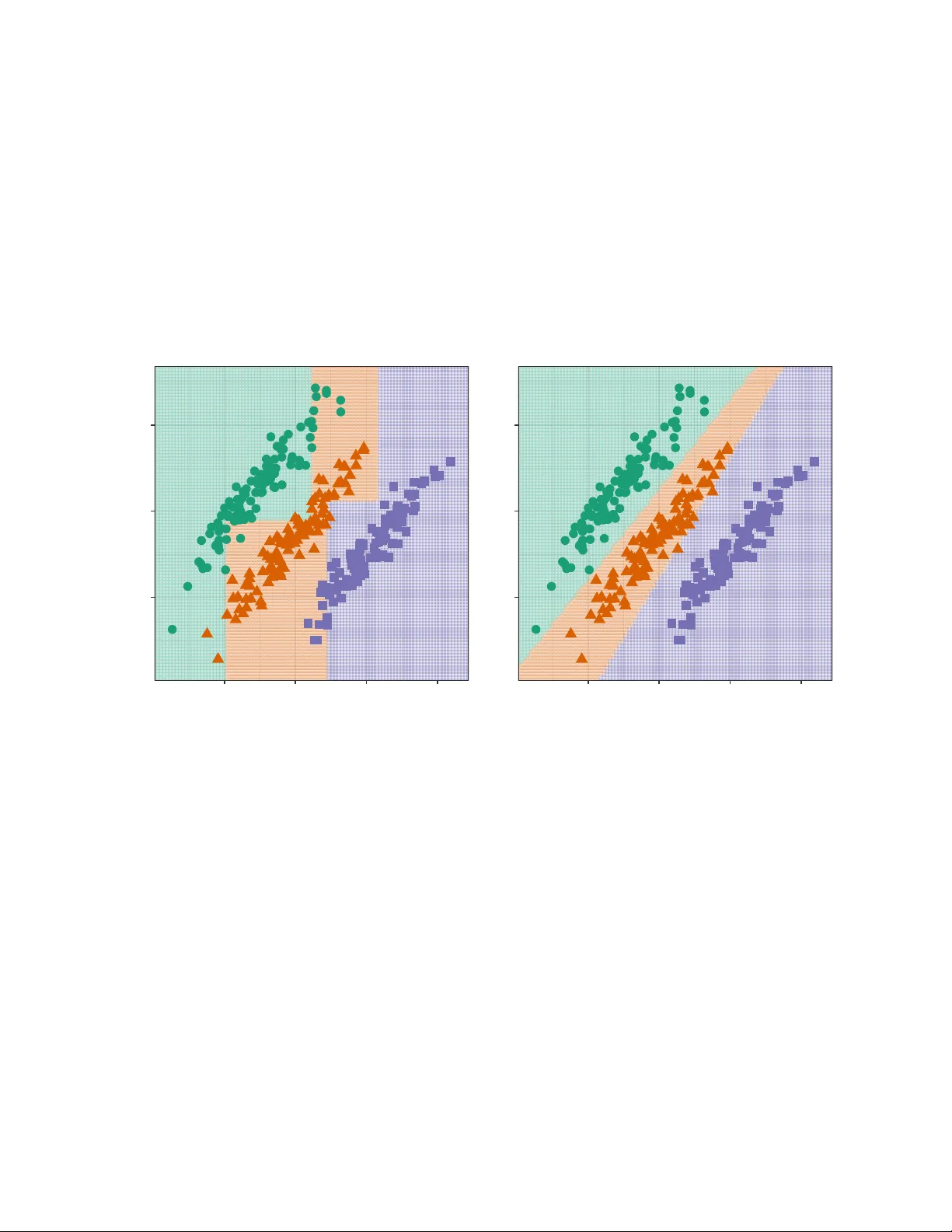
An Enhanced Pro jection Pursuit T ree Classier with Visual Metho ds for Assessing Algorithmic Impro v emen ts Natalia da Silv a Dianne Co ok Eun-Kyung Lee Abstract This pap er presen ts enhancements to the projection pursuit tree classier and vi- sual diagnostic metho ds for assessing their impact in high dimensions. The original algorithm uses linear com binations of v ariables in a tree structure where depth is con- strained to be less than the n um ber of classes—a limitation that pro ves too rigid for complex classication problems. Our extensions improv e p erformance in multi-class settings with unequal v ariance-co v ariance structures and nonlinear class separations b y allo wing more splits and more exible class groupings in the pro jection pursuit compu- tation. Prop osing algorithmic improv emen ts is straigh tforward; demonstrating their actual utilit y is not. W e therefore develop tw o visual diagnostic approaches to ver- ify that the enhancements p erform as intended. Using high-dimensional visualization tec hniques, w e examine mo del ts on benchmark datasets to assess whether the algo- rithm b ehav es as theorized. An interactiv e web application enables users to explore the b ehavior of b oth the original and enhanced classiers under con trolled scenarios. The enhancements are implemen ted in the R package PPtreeExt . 1 In tro duction Loh (2014) pro vides an extensiv e o v erview of decades of researc h on classication and re- gression tree algorithms. T ree mo dels are useful b ecause they are simple, yet exible, fast to compute, widely applicable and interpretable. A main drawbac k, though, most av ailable metho ds use splits along single v ariables, which means that separations b est made using a com bination of v ariables are awkw ard for trees to t. While there hav e b een man y sugges- tions it is a muc h harder problem to optimize on linear combinations, and thus there is less a v ailable successful soft w are for oblique splits. One av ailable metho d and soft w are is the Pro jection Pursuit T ree (PPtree) algorithm (Y. D. Lee et al. 2013). It optimizes a projection pursuit index, for example the LDA (E.-K. Lee et al. 2005) or PD A (E.-K. Lee and Cook 2010) index among others, based on class information to iden tify one-dimensional projections that b est separate the groups at eac h no de. The PPtree tree structure is simpler than classic metho ds like rpart (Therneau and A tkinson 2025), as it restricts the depth to ( is the n umber of classes). At eac h no de, PPtree separates the data in to t w o groups by rst deciding whic h classes to group together; 1 the data are split into left and right branches based on tw o group means. This pro duces a compact and interpretable tree implemen ted in PPtreeViz R package (E.-K. Lee 2018). One of the main adv antages of PPtree is its ability to leverage the correlation b et ween predictor v ariables to improv e class separation. It has b een shown to outperform even random forests (RF) in some scenarios. Pro jection pursuit addresses a known limitation of the original RF algorithm, in whic h oblique projections w ere allow ed. While it sounds app ealing, the algorithm is practically infeasible b ecause it is based on randomly generated splits. Thus it is slo w, and inecient, for nding useful separating oblique splits. The compact nature of PPtree means that it ts simply , and do es not require pruning. The resulting one-dimensional pro jections can b e used to make visualizations of group separations. Ho w ev er, there are limitations that reduce its eectiv eness in certain contexts. Due the the wa y classes are group ed, the prediction b oundaries are often too close to one group, resulting in unnecessarily high error rates. This happ ens b ecause grouping of classes lik ely pro duces unequal v ariance-cov ariances, making the p o oled v ariance-co v ariance used by LD A inadequate. Moreo ver, when classes hav e non-elliptical v ariance-cov ariance, or are split in to m ultiple clusters, the rigidit y of the -1)-no de structure, will not b e suciently exible. A primary ob jectiv e of this pap er is to describ e mo dications to the PPtree algorithm that address these limitations. The algorithm is changed in tw o w ays: (1) improving prediction b oundaries by mo difying the choice of split p oints-through class subsetting; and (2) increas- ing exibility b y allo wing multiple splits p er group. The mo died algorithm is tested on a v ariety of b enchmark data sets. These data sets include w ell-separated classes, the presence of outliers, and nonlinear b oundaries. The p erformance is compared with the original PP- tree algorithm and existing metho ds. Visual comparisons of decision b oundaries, along with error rates, are used to further understand the mo del ts. The ultimate goal is to provide b etter building blo c ks for a pro jection pursuit-based classication random forest algorithm (da Silv a, Co ok, and Lee 2021) implemented in PPforest R package (da Silv a, Co ok, and Lee 2025). Prop osing enhancemen ts to algorithms is easy , and theoretically the mo dications ma y seem sensible. In practice, they may not work as one en visions. Th us, an imp ortan t part of devel- oping algorithm mo dications is providing v alidation that they are doing what is exp ected. This means going b eyond predictive accuracy , to understanding the resulting mo dels. A sec- ond ob jectiv e of this pap er is to provide visual diagnostics for the algorithm changes. This is tw o-fold: a shin y (Chang et al. 2025) app and tours to view the ts in high dimensions. The app is a v ailable in the PPtreeExt package (da Silv a, Co ok, and Lee 2026) along with the implemen tation of the mo died algorithm. It allo ws users to generate 2D data sets with dieren t types of separations and compare the mo del ts for the mo died and the original algorithm. This was an essential to ol in constructing the new algorithm, b ecause it provides side-b y-side visualization of prediction b oundaries to identify data patterns in which the dieren t metho ds p erform b etter. The second visual diagnostic is to use tours av ailable in the tourr pac kage (Wickham et al. 2011) to examine the high-dimensional structure of data sets and the resulting mo del ts where the mo died algorithm outp erforms other classiers. This pro vides an explanation for the p erformance comparison results, and intuition for why the mo died algorithm p erforms b etter. 2 The paper is organized as follo ws: Section 2 pro vides bac kground on the original PPtree algorithm, including its structure and limitations. Section 3 describ es the extensions to the algorithm. Section 4 presen ts the interactiv e visualization to ol developed for exploring and comparing the algorithms. Section 5 presents the comparativ e analysis of algorithm p erformance, and visual diagnostics for the comparisons in Section 6 . Finally , Section 7 discusses the changes, results of the comparison and p otential future directions. 2 Bac kground to PPtree Figure 1 illustrates the original PPtree algorithm for . Starting from the optimal pro jection, the green group-ha ving the most distant mean—is relab eled as , while the orange and violet groups are com bined and relab eled as . A second pro jection vector is then computed using all observ ations, follo wing the same pro cedure applied to these t wo new sup er-groups. A split point is determined using one of the predened rules, and observ ations are assigned to branc hes by comparing their pro jected v alues to the cuto. The algorithm computes a split p oint using one of sev eral metho ds and the observ ations are allo cated to groups based on whether their pro jected v alues fall b elo w or ab ov e the cuto. Since con tains only one of the original classes, the left branc h b ecomes a terminal no de. Because still includes tw o original classes, the pro cedure is recursively rep eated on the righ t branch. There are eight dierent rules a v ailable for computing the split p oint on a given pro jection. Let x , x , , , and denote the mean, median, standard deviation, in terquartile range, and sample size of group , respectively . T able 1 summarizes the form ulas used to calculate the split p oin t v alue, , under each rule. T able 1: Rules for computing the split v alue, , b etw een tw o groups, on a data pro jection, using means, weigh ted mean, medians, standard deviations, in terquartile ranges. R ule Name F ormula 1 mean x x 2 sample size weigh ted mean x x 3 standard deviation w eigh ted mean x x 4 standard error w eigh ted mean x x 5 median 6 sample size weigh ted median 7 IQR weigh ted median 3 R ule Name F ormula 8 sample size and IQR w eigh ted median 2.1 Algorithm The PPtree algorithm (Y. D. Lee et al. 2013) follo ws a m ulti-step pro cedure to identify linear combinations of predictors that optimally separate classes in multi-class settings. Let x denote the dataset, where x is a -dimensional v ector of explanatory v ariables. The corresp onding class lab el is , with , for . The construction of a PPtree classier follows a four-step algorithm, describ ed as follo ws: PPtree Algorithm (4-step v ersion) Input: Dataset x , with x , Output: A pro jection pursuit classication tree with at most internal no des • Step 1: Class Separation. Optimize a pro jection pursuit index (e.g., LD A or PDA) to nd a pro jection v ector that b est separates all classes in the current no de. • Step 2: Binary Relab eling. On pro jected data, x , compute pro jected class means . Iden tify the pair with the largest mean dierence and compute the midp oin t . Relab el the observ ations into t w o sup er-classes, and , dep ending on whether is smaller than the midp oint . • Step 3: No de Splitting. Optimize a new pro jection to separate and based on the relab eled classes. Dene the split v alue on x using a predened rule (e.g., mean or w eigh ted mean). Split the no de using the rule . • Step 4: Recursiv e Partitioning. Rep eat Steps 1–3 for each c hild no de un til every terminal no de contains only one original class. 2.2 Less desirable asp ects The decision b oundaries of a classier reect how the mo del partitions the feature space and adapt to class separations. Visualizing the decision boundaries pro vides v aluable in- sigh ts into mo del b ehavior and limitations. T o illustrate the motiv ation for extending the PPtree algorithm, w e present simple examples based on simulated datasets. Details on the sim ulation settings are pro vided in Section 4 . Figure 2 shows the decision boundaries pro duced b y rpart (left) and PPtree (right). In this example, the class structure is b est separated using linear com binations of the tw o v ariables. The rpart algorithm, whic h relies on axis-aligned splits, must appro ximate the ideal b oundary using multiple steps. In con trast, PPtree generates an oblique split that more eectiv ely captures the separation, although the resulting b oundary b etw een the orange and purple classes lies to o close to one of them. 4 Stratified bootstrap samples by classStratified bootstrap samples by class bootstrap samples by class T raining data Step 1: find the optimal1-D Projection and pr oject the data — z 1 — z 2 — z 3 Step 2: mean for each class is computed g=1 g=2 g=3 g* 1 g* 2 using the distance among means redefine the problem in two class Step 3: find the optimal 1-D Projection to separate g* 1 and g* 2 Final node Step 4: repeat step 1 to 3 Figure 1: Illustration of the original PPtree algorithm for . 5 The rst split isolates the violet class from the other tw o. A second partition then attempts to separate the green and orange groups. Although the group structure is similar across the three classes, the resulting decision b oundaries are not parallel. This o ccurs b ecause the initial split uses the combined information from the orange and green groups-treated as a sup er-group—to compute the pro jection and determine the splitting p oint. Alternativ e rules for computing the split v alue (see T able 1 ) hav e a substantial impact on the p osition and orien tation of these decision b oundaries. −2 0 2 −2 0 2 4 Rpar t error 7.3 % −2 0 2 −2 0 2 4 PPtree error 0.7 % Figure 2: Comparison of decision b oundaries pro duced by the rpart (left) and PPtree (righ t) algorithms on tw o-dimensional simulated data. The b oundaries generated by PPtree are oblique to the co ordinate axes, capturing the linear asso ciation betw een the tw o v ariables. Figure 3 displays a sim ulated example that highligh ts the limited exibilit y of the decision b oundaries pro duced b y PPtree . In this scenario, the orange class cannot b e separated using a single linear partition, and PPtree fails to mo del it accurately b ecause eac h original class must b e assigned to a single terminal no de. In con trast, the more traditional rpart algorithm p erforms b etter in this case, as its recursive structure allo ws it to accommo date the relatively simple non-linear separation. 3 PPtree extensions The algorithm has b een extended in tw o main wa ys: by mo difying the rules used to determine decision b oundaries and by allo wing multiple splits per group. T wo new approaches are 6 −2.5 0.0 2.5 5.0 −2 0 2 4 Rpar t error 5 % −2.5 0.0 2.5 5.0 −2 0 2 4 PPtree error 23.8 % Figure 3: Comparison of decision b oundaries pro duced b y the rpart (left) and PPtree (right) algorithms on tw o-dimensional sim ulated data. The orange class cannot b e separated using a single linear partition, and PPtree fails to mo del it accurately b ecause each original class m ust b e assigned to a single terminal no de. 7 in tro duced for computing the optimal split v alue. T o supp ort multiple splits within a group, additional stopping rules m ust b e incorp orated in to the algorithm. 3.1 Mo dication 1: Subsetting classes to pro duce b etter b oundaries The rst mo dication targets the third step of the original algorithm. Rather than combining all remaining classes into a single sup er-class, only the tw o closest ones—identied by the smallest dierence in their pro jected means—are used to compute the next pro jection and dene the split p oin t Find an optimal one-dimensional pro jection , using a subset of x i to separate the tw o class problem and . T o this second pro jection only information from the t w o closest groups, one from and the other from are used. The b est separation of and is determined by x ; then is assigned to the left no de else assign to the righ t no de, where x is the mean of . Figure 4 illustrates the mo died v ersion of the algorithm for a three-class classication problem. After identifying the initial optimal pro jection, instead of com bining tw o groups in to a single sup er-group, the group furthest from the others is temp orarily excluded. In this example, class is dropp ed from the current no de. A new pro jection is then computed using only classes and (relab eled as and ), and one of the eigh t a v ailable rules is applied to determine the optimal split p oint. Subsequently , class is reintroduced, and a new pro jection is computed to b est separate it from , completing the tree construction. Figure 6 sho ws the eect of this mo dication on the decision b oundaries obtained from the sim ulated dataset presented in Figure 2 . 3.2 Mo dication 2: Multiple splits p er class based on en trop y reduction This mo dication introduces a new approac h for selecting the split v alue, based on the impurit y of the resulting groups. This approach resem bles the impurit y-based criteria used in the rpart algorithm, but it op erates on pro jected data rather than individual features. Curren tly , the only implemented impurity measure is negative entrop y: log (1) where is the prop ortion of observ ations from class in subset , and is the n umber of classes. Higher v alues of indicate greater class impurity . When all observ ations in the subset belong to the same class, the en trop y reac hes its minim um v alue of , indicating a pure no de. T o ev aluate the quality of a candidate split, the impurity v alues of the resulting left and righ t subsets are com bined using a w eighted av erage of the entropie: (2) 8 Stratified bootstrap samples by classStratified bootstrap samples by class bootstrap samples by class T raining data Step 1: find the optimal1-D projection and pr oject the data Step 2: mean for each class is computed and the entropy in the middle point between group mean using the distance among means redefine the problem in two class. g1 g2 g3 Step 3: Find the optimal 1-D projection to separate g* 1 and g* 2 but only using information of the closest groups in g* 1 and g* 2 Final node Differ ent from original PPtree — z 1 — z 2 — z 3 g* 1 g* 2 Step 4: Repeat step 1 to 3 Figure 4: Illustration of the algorithm with Mo dication 1 applied to a three-class problem. A t each no de, the second one-dimensional pro jection is computed using only the tw o closest groups to determine the b est pro jection direction and split p oin t. 9 where are the num b er of observ ations in the left and righ t subsets, respectively . The combined impurity , is computed for all p ossible split points-dened as the midp oin ts b et w een consecutiv e ordered pro jected v alues-denoted . The split p oint that minimizes the combined entrop y is selected: min This represen ts a ma jor departure from the original PPtree structure, aiming to enhance exibilit y in mo deling non-linear class b oundaries b y allowing m ultiple splits within a class. Instead of relying on summary statistics at the class lev el, this approach shifts the fo cus to lo cal dierences b etw een individual observ ations. T o supp ort this exibility , additional con- trol mechanisms are required, particularly new stopping criteria. While this is conceptually similar to the rpart algorithm, a k ey distinction is that larger sample sizes p er no de are needed to reliably estimate pro jection co ecients. Figure 5 illustrates this mo died version of the algorithm, which follows the steps outlined b elo w. PPtree Algorithm with En trop y-Based Splitting Input: Dataset x , with x , Output: A pro jection pursuit classication tree with en tropy-based no de splitting • Step 1: Class Separation. Optimize a pro jection pursuit index (e.g., LD A or PDA) to nd a pro jection v ector that b est separates the classes in the current no de. • Step 2: Pro jection and Candidate Splits. On the pro jected data, x , dene candidate splits as midp oin ts b etw een consecutiv e v alues. • Step 3: Impurit y Ev aluation. F or eac h candidate split , divide the data in to and . Compute the class prop ortions for eac h subset and ev aluate the en trop y: log Compute the total impurit y as: • Step 4: Best Split Selection. Select the split p oint that minimizes . Split the no de using the rule . • Step 5: Recursive Partitioning. Rep eat Steps 1–4 recursively on each child no de un til some of the follo wing stopping criteria are met: – All observ ations in the no de b elong to the same class; 10 – The no de size is smaller than a minimum threshold ; – The entrop y reduction is smaller than a threshold . Stratified bootstrap samples by classStratified bootstrap samples by class bootstrap samples by class T raining data Step1: find the optimal1-D projection and pr oject the data Step2: compute the entropy in each possible partition (between each observation) g1 g2 g3 Step 3: Select the partition with the minimum entropy T erminal node Step 4: Repeat step 2 and 3 until stopping rules are hold Step1: find the optimal1-D Projection and pr oject the data e21,e22 e11,e12 e31,e32 e41,e42 e51,e52 e61,e62 Compute ei1, ei2 for all the partitions T erminal node Figure 5: Illustration of the algorithm with Mo dication 2 applied to a three-class problem. Pro jections of the data are computed at each no de, and multiple splits p er class are allo wed. An impurit y-based criterion, suc h as entrop y , is used to determine when and ho w often to split observ ations within a no de. 4 Algorithm comparison T o ev aluate b oth the original algorithm and the prop osed modications, w e developed an in teractiv e Shiny app (Chang et al. 2025). The tool includes metho ds for simulating 2D classication problems, and displays the decision b oundaries generated b y dierent algo- rithms: CAR T, PPtree, and the prop osed extensions (implemen ted in rpart , PPtreeViz , and PPtreeExt , resp ectiv ely). The Shiny app is av ailable at h tt ps : // na ty ds .s hi ny ap ps .i o/ explorapp/ and is implemen ted in PPtreeExt . The app con tains three tabs, each tab oers control o v er data generation and algorithm parameters: Basic-Sim, Sim-Outlier, and MixSim. The rst tab sim ulates w ell-separated 11 classes, the second includes a cluster of outliers, and the third generates ov erlapping groups using the MixSim package (Melnyk o v, Chen, and Maitra 2012). Each tab oers con trol o v er data generation and algorithm parameters. The decision b oundaries for rpart , PPtree , and the mo died PPtree are display ed side b y side for visual comparison. A dditional con trols, suc h as the rule partition used in PPtree algorithm and the mo died PPtree based on subsetting clases, can b e incorp orated in to the application. These features allo w users to examine ho w changes in rule criteria inuence the resulting classication b oundaries. Figure 6 illustrates the use of the in teractiv e application. The rst mo dication (Subset- ting clases) is applied to generate the pro jection, and Rule 1 is used to compute the split p oin t. The mo died PPtree achiev es an error rate comparable to the original PPtree , with b oth substan tially outperforming rpart . Additionally , the resulting decision boundary more accurately partitions the groups in a balanced manner. Figure 6: Model ts for the three algorithms— rpart , PPtree , and the modied PPtree based on subsetting clases applied to simulated w ell-separated classes. F or PPtree , Rule 1 is used to determine the split p oints. The mo died PPtree pro duces decision b oundaries that are more symmetrically placed b etw een the clusters. Figure 7 presents a scenario in which Mo dication 2 (Multiple splits) yields a substan tial impro v emen t ov er the other algorithms. The use of multiple splits enables the small group of outliers from class 2 to b e correctly classied. Figure 8 compares the p erformance of the algorithm v ariants on data sim ulated from Gaus- sian mixtures. The user can adjust sev eral parameters of the mixture model: is the sample 12 Figure 7: Model ts for the three algorithms—rpart, PPtree, and the mo died PPtree— applied to data in whic h one class consists of t w o distinct clusters. The b oundaries pro duced b y the mo died PPtree with multiple splits b etter capture the underlying structure of the data compared to the other metho ds. 13 size, is the desired av erage ov erlap b et ween comp onents, sp ecies the maximum allow able o v erlap, and is the n um b er of groups. Figure 8: Decision b oundaries pro duced b y the three algorithms— rpart, PPtree, and the mo died PPtree—on data sim ulated from a Gaussian mixture mo del. The interactiv e application pro vides insight into ho w mo dications to the algorithm aect mo del t. It follows the principle of visualizing the mo del in the data space (Wic kham, Cook, and Hofmann 2015). An additional and imp ortan t use of the tool has been for debugging and ev aluating the algorithmic behavior. By adjusting the sim ulated data and model parameters, it b ecomes evident that small c hanges in the data can result in substantial c hanges in the tted mo del—particularly when pro jections are inv olv ed. This sensitivity is likely to b e even greater in higher-dimensional settings. Ho w ev er, in scenarios where class separation o ccurs along combinations of v ariables, the use of pro jected data at each no de tends to yield decision b oundaries that more closely align with the true data distribution. 14 5 P erformance comparison This section presents a b enc hmark data study to ev aluate the predictiv e p erformance of the prop osed metho d. W e compare the extended PPtree mo dels with several classica- tion metho ds—CAR T, PPtree, Random F orest, PPforest, and SVM—using 94 b enchmark datasets. T able 3 in the App endix con tain the url with the source data while T able 6 sum- marize the main characteristics of eac h dataset summarizing the n um b er of observ ations, predictors, n umber of classes, class imbalance, and absolute av erage correlation among pre- dictors. Im balance quanties the disparity in class sizes (0 indicates p erfectly balanced classes, biggest prop ortion size dierence b et ween classes), while higher correlation suggests a greater p otential for class separation through linear combinations of v ariables. F or eac h dataset, tw o-thirds of the observ ations are randomly selected for training, and the remaining one-third is used for testing and computing the prediction error. This pro cess is rep eated 200 times. data22−1 data49−4 data56−1 data67 data69−1 data69−2 data37−5 data38 data63 data34 data49−2 data49−3 data20−3 data27−a11 data27−a31 data27−b31 data27−c11 data27−c31 0.050 0.075 0.100 0.125 0.150 0.2 0.3 0.4 0.5 0.05 0.10 0.15 0.3 0.4 0.5 0.200 0.225 0.250 0.275 0.20 0.22 0.24 0.26 0.02 0.04 0.06 0.4 0.5 0.6 0.04 0.05 0.06 0.07 0.08 0.00 0.02 0.04 0.2 0.3 0.4 0.2 0.3 0.4 0.5 0.010 0.015 0.020 0.025 0.15 0.20 0.25 0.30 0.15 0.20 0.25 0.30 0.2 0.3 0.4 0.5 0.25 0.30 0.35 0.40 0.20 0.25 0.30 0.35 0.40 rpar t PPtree (lda) PPtree (pda) PPtreeExt (mod 1) PPtreeExt (mod 2) rpar t PPtree (lda) PPtree (pda) PPtreeExt (mod 1) PPtreeExt (mod 2) rpar t PPtree (lda) PPtree (pda) PPtreeExt (mod 1) PPtreeExt (mod 2) A verage test error Figure 9: A verage test error from 200 training/test splits of b enchmark data for four mo dels: rpart, PPtree PPtreeExt mo dications 1 and 2, where the PPtree extension p erforms b etter than rpart and the original PPtree. Moreo v er, in 18 datasets, the modied PPtree outp erforms CAR T, as illustrated in Fig- ure 9 , and in only 3 cases it achiev es the low est error among all selected metho ds, including ensem ble-based classiers. T able 2 presents an ov erview of these datasets, which is a subset of T able 6 from the App endix. 15 T able 2: Ov erview of b enc hmark datasets where the prop osed tree-based extensions outp er- form the selected tree metho ds. The table summarizes the num b er of observ ations, predictors, n um b er of classes, class imbalance, and absolute a v erage correlation among predictors. Im- balance quanties the disparit y in class sizes (0 indicates p erfectly balanced classes), while higher correlation suggests a greater p otential for class separation through linear com bina- tions of v ariables. dataset Cases Predictors Groups Im balance Correlation data20-3 8143 5 2 0.58 0.45 data27-a11 1747 18 5 0.38 0.24 data27-a31 1834 18 5 0.28 0.27 data27-b31 1424 18 5 0.21 0.24 data27-c11 1111 18 5 0.14 0.27 data27-c31 1448 18 5 0.17 0.27 data37-5 17560 53 5 0.21 0.16 data38 182 12 2 0.43 0.21 data63 6598 166 2 0.69 0.27 data34 1372 4 2 0.11 0.43 data49-2 606 100 2 0.03 1.00 data49-3 606 100 2 0.01 0.99 data22-1 258 5 4 0.25 0.12 data49-4 606 100 2 0.01 0.99 data56-1 7494 16 10 0.01 0.27 data67 20000 16 26 0.00 0.18 data69-1 5000 21 3 0.01 0.30 data69-2 5000 40 3 0.01 0.09 6 Explanation of p erformance W e w ould exp ect that the mo died PPtree algorithm outp erforms • rpart when the b est separation b etw een groups is in oblique directions • and the original PPtree when class v ariances are dierent, or when there are multiple classes. This can b e inv estigated visually using a tour. There are several strategies for approaching this: 1. On the data a. W ork on t w o groups at a time, if there are more than 2 b. Use a guided tour on the data to nd the combinations of the v ariables where the groups are separated 2. Predict a grid of v alues that co v ers the data domain, for the metho ds in terested in comparing, PPtreeExt, rpart and PPtree a. subset to the p oints near the b order generated b y the classier. 16 b. record a sequence of pro jection bases that shows the b oundary created by PPtree c. use the same pro jection sequence to view the b oundaries for the three dieren t metho ds, p ossibly use a slice tour to fo cus on the b oundary near the cen ter of the data domain. Figure 10 show pro jections of the data20-3 illustrating why PPtreeExt p erforms b etter. Group 0 is split on either side of group 1, whic h means that the original PPtree algorithm w ould not b e able to capture b oth clusters. W e can also see that the separation is mostly on V3 but small amounts of other v ariables help to improv e the separation. This means that rpart will not w ork quite as w ell b ecause it will fo cus on splitting V3 . (a) pro jection 1 (b) pro jection 2 Figure 10: T w o pro jections from a grand tour of data20-3, from whic h we can see why the PPtreeExt metho d is the most eectiv e. The group 0 is split in to t wo clusters on either side of group 1, which means that the original algorithm is not optimal. Secondly , the separation b et w een the t w o groups is in a combination of v ariables. Figure 11 sho ws some plots illustrating why PPtreeExt outperforms the other methods of the data49-2 data. F rom Figure 9 w e can see that the original PPtree (with LDA) algorithm p erforms muc h b etter than a tree, and the PPtreeExt p erforms muc h b etter again. This data has 100 predictors and 2 classes (T able 2 ), whic h makes visualising more challenging that data20-3 . A useful approac h is to pre-pro cess using principal comp onent analysis (PCA) on the predictors, to reduce the n um b er of v ariables to visualise, while maintaining class structure. Plot (a) shows PC 1 vs PC2, with p oin ts coloured by the tw o classes. PC 1 explains 99.8% of the v ariability in the predictors but it explains nothing of the class structure. This is not uncommon for PCA, where often in teresting structure can b e found in the smaller comp onents. Plot (b) shows PC 2 vs PC 3, and here we see interesting class dierences. Each class app ears to hav e three linear pieces p oin ting in dieren t directions. This supp orts why PPtreeExt migh t work well, b ecause in the combination of v ariables, the 17 classes are nearly separable with m ultiple linear cuts. It’s not feasible to contin ue w orking through principal comp onents to tease apart the cluster structure relating to classes, so a go o d next step is to do pro jection pursuit. The optimal pro jection is shown in plot (c). It can b e seen the t wo classes are mostly separable by a linear combination of v ariables, but there is no gap b etw een the clusters. The linear combination with so man y v ariables is what causes some diculties for a simple tree algorithm. The interesting shap es of the clusters for each class, which app ear to b e multiple linear pieces, means that the PPtreeExt can nd b etter separations than PPtree. (a) PC1 vs PC2 (b) PC2 vs PC3 (c) optimal pro jection Figure 11: Examining wh y data49-2 is b est classied using PPtreeExt. Because there are 100 predictors, for visualisation it is useful to reduce the dimension using principal comp onen t analysis, and then examine the separation b etw een groups. PC1 explains 99.8% of the ov erall v ariability among predictors, but it is not useful for separating the classes (a). PC2 and PC3 (b) hav e an interesting dierence b et w een the tw o classes which shows why multiple linear splits migh t b e useful. A guided pro jection pursuit on the rst 26 principal comp onen ts (c) sho ws that these classes could b e separated with a linear combination. This is why the original PPtree classier does b etter than the tree algorithm and also wh y the extension impro v es the p erformance. Figure 12 has plots illustrating wh y the PPtreeExt p erforms b etter on data69-1 . F rom Figure 9 we see that all of the PPtree versions p erform b etter than an rpart t. This data has 21 predictors and 3 classes (T able 2 ). This is sucien tly small to examine using a tour, and we initially use a guided tour with the LD A index. This pro duced the pro jection shown in plot (a) where we see the primary dierence b etw een the three classes. These are each similar size, but orien ted in suc h a w a y that in a 2D pro jection they form a triangle. Plots (b) and (c) show the b oundaries using a slice tour with the same pro jection as used in (a) for PPtreeExt and rpart, resp ectively . The b oundary p oin ts are generated by sim ulating a random sample of observ ations b et ween (-3, 3) in each dimension. The slice cuts through to cen tre of the b ox. W e can see that PPtreeExt essen tially ts the data shap e neatly but the rpart b oundary is very messy . This data needs oblique cuts, which PPtreeExt provides, and the mo died algorithm handles the v ariance dierences b etter than the original. 18 (a) data (b) PPtreeExt (c) rpart Figure 12: Examining why data49-2 is b est classied using PPtreeExt: (a) b est pro jection from a guided tour shows that the data has three similar linear pieces orien ted to form a triangle, (b) b oundary pro duced b y the PPtreeExt tted mo del and (c) b oundary pro duced b y rpart tted mo del. 7 Discussion This article has presented tw o mo dications to the PPtree algorithm for classication prob- lems implemented in the R pac kage PPtreeExt and ev aluated using a purp ose-built interac- tiv e web application and real data. The rst mo dication in v olv es subsetting classes when calculating the pro jection direction at each no de, while the second allo ws for multiple splits p er class based on individual en trop y ev aluations b et ween candidate splits. These changes result in a more exible classication metho d that leverages linear com binations of v ariables. The w eb application also demonstrates how easily diagnostic to ols can b e constructed to explore and understand the b ehavior of new algorithms. The b enchmark data study show ed that PPtreeExt predictive p erformance is b etter than, CAR T and PPtree in 18 data out of 94. The mo died PPtree algorithm outp erforms CAR T in cases when the b est separation b etw een groups is in oblique directions and outp erforms the original PPtree when class v ariances are dierent, or when there are multiple classes. In terpretabilit y is increasingly imp ortan t, b ecause predictions from algorithms ma y need to b e defended in practice. W e hav e shown ho w to examine the data and the tted mo del to understand wh y the PPtree extension performs b etter than other tree metho ds on some data sets. This approach is generally useful for assessing and diagnosing mo del ts. The mo died tree algorithm can be incorporated in to a pro jection pursuit forest classier (da Silv a, Co ok, and Lee 2025). Giv en its implicit v ariable selection mechanism, the ensemble is exp ected to handle n uisance v ariables more eectiv ely than a single tree. A dditionally , the use of bagging should yield improv ed and more robust p erformance in problems with nonlinear decision boundaries. This can be accomplished using the curren t PPforest pac kage. 8 App endix 19 T able 3: Source data information Name URL data12 h ttps://archiv e.ics.uci.edu/dataset/518/sp eaker+accen t+recognition data13-1 h ttps://archiv e.ics.uci.edu/dataset/547/algerian+forest+res+dataset data13-2 h ttps://archiv e.ics.uci.edu/dataset/547/algerian+forest+res+dataset data20-1 h ttps://archiv e.ics.uci.edu/dataset/357/o ccupancy+detection data20-2 h ttps://archiv e.ics.uci.edu/dataset/357/o ccupancy+detection data20-3 h ttps://archiv e.ics.uci.edu/dataset/357/o ccupancy+detection data21 h ttps://archiv e.ics.uci.edu/dataset/537/cervical+cancer+b ehavior+risk data22-1 h ttps://archiv e.ics.uci.edu/dataset/257/user+knowledge+modeling data22-2 h ttps://archiv e.ics.uci.edu/dataset/257/user+knowledge+modeling data26 h ttps://archiv e.ics.uci.edu/dataset/308/gas+sensor+array+under+o w+mo dulation data27-a11 h ttps://archiv e.ics.uci.edu/dataset/302/gesture+phase+segmentation data27-a21 h ttps://archiv e.ics.uci.edu/dataset/302/gesture+phase+segmentation data27-a31 h ttps://archiv e.ics.uci.edu/dataset/302/gesture+phase+segmentation data27-a32 h ttps://archiv e.ics.uci.edu/dataset/302/gesture+phase+segmentation data27-b11 h ttps://archiv e.ics.uci.edu/dataset/302/gesture+phase+segmentation data27-b12 h ttps://archiv e.ics.uci.edu/dataset/302/gesture+phase+segmentation data27-b31 h ttps://archiv e.ics.uci.edu/dataset/302/gesture+phase+segmentation data27-b32 h ttps://archiv e.ics.uci.edu/dataset/302/gesture+phase+segmentation data27-c11 h ttps://archiv e.ics.uci.edu/dataset/302/gesture+phase+segmentation data27-c12 h ttps://archiv e.ics.uci.edu/dataset/302/gesture+phase+segmentation data27-c31 h ttps://archiv e.ics.uci.edu/dataset/302/gesture+phase+segmentation data27-c32 h ttps://archiv e.ics.uci.edu/dataset/302/gesture+phase+segmentation data29 h ttps://archiv e.ics.uci.edu/dataset/282/lsvt+voice+rehabilitation data32 h ttps://archiv e.ics.uci.edu/dataset/257/user+knowledge+modeling data34 h ttps://archiv e.ics.uci.edu/dataset/267/banknote+authentication data36 h ttps://archiv e.ics.uci.edu/dataset/236/seeds data37-1 h ttps://archiv e.ics.uci.edu/dataset/231/pamap2+physical+activit y+monitoring data37-2 h ttps://archiv e.ics.uci.edu/dataset/231/pamap2+physical+activit y+monitoring data37-3 h ttps://archiv e.ics.uci.edu/dataset/231/pamap2+physical+activit y+monitoring data37-4 h ttps://archiv e.ics.uci.edu/dataset/231/pamap2+physical+activit y+monitoring data37-5 h ttps://archiv e.ics.uci.edu/dataset/231/pamap2+physical+activit y+monitoring data37-8 h ttps://archiv e.ics.uci.edu/dataset/231/pamap2+physical+activit y+monitoring data37-14 h ttps://archiv e.ics.uci.edu/dataset/231/pamap2+physical+activit y+monitoring data38 h ttps://archiv e.ics.uci.edu/dataset/230/planning+relax data39-1 h ttps://archiv e.ics.uci.edu/dataset/224/gas+sensor+array+drift+dataset Name URL data39-2 h ttps://archiv e.ics.uci.edu/dataset/224/gas+sensor+array+drift+dataset data39-3 h ttps://archiv e.ics.uci.edu/dataset/224/gas+sensor+array+drift+dataset data39-4 h ttps://archiv e.ics.uci.edu/dataset/224/gas+sensor+array+drift+dataset data39-5 h ttps://archiv e.ics.uci.edu/dataset/224/gas+sensor+array+drift+dataset data39-6 h ttps://archiv e.ics.uci.edu/dataset/224/gas+sensor+array+drift+dataset data39-7 h ttps://archiv e.ics.uci.edu/dataset/224/gas+sensor+array+drift+dataset 20 data39-8 h ttps://archiv e.ics.uci.edu/dataset/225/gas+sensor+array+drift+dataset data39-9 h ttps://archiv e.ics.uci.edu/dataset/226/gas+sensor+array+drift+dataset data41-1 h ttps://archiv e.ics.uci.edu/dataset/194/wall+follo wing+rob ot+na vigation+data data41-2 h ttps://archiv e.ics.uci.edu/dataset/194/wall+follo wing+rob ot+na vigation+data data41-3 h ttps://archiv e.ics.uci.edu/dataset/194/wall+follo wing+rob ot+na vigation+data data42 h ttps://archiv e.ics.uci.edu/dataset/192/breast+tissue data44 h ttps://archiv e.ics.uci.edu/dataset/181/libras+mov ement data49-2 h ttps://archiv e.ics.uci.edu/dataset/167/hill+v alley data49-3 h ttps://archiv e.ics.uci.edu/dataset/168/hill+v alley data49-4 h ttps://archiv e.ics.uci.edu/dataset/169/hill+v alley data50 h ttps://archiv e.ics.uci.edu/dataset/161/mammographic+mass data52-1 h ttps://archiv e.ics.uci.edu/dataset/96/sp ectf+heart data52-2 h ttps://archiv e.ics.uci.edu/dataset/96/sp ectf+heart data53 h ttps://archiv e.ics.uci.edu/dataset/139/synthetic+con trol+chart+time+series data55-1 h ttps://archiv e.ics.uci.edu/dataset/80/optical+recognition+of+handwritten+digits data55-2 h ttps://archiv e.ics.uci.edu/dataset/80/optical+recognition+of+handwritten+digits data56-1 h ttps://archiv e.ics.uci.edu/dataset/81/p en+based+recognition+of+handwritten+digits data56-2 h ttps://archiv e.ics.uci.edu/dataset/81/p en+based+recognition+of+handwritten+digits data57 h ttps://archiv e.ics.uci.edu/dataset/39/ecoli data61-1 h ttps://archiv e.ics.uci.edu/dataset/54/isolet data62 h ttps://archiv e.ics.uci.edu/dataset/74/musk+v ersion+1 data63 h ttps://archiv e.ics.uci.edu/dataset/75/musk+v ersion+2 data64-1 h ttps://archiv e.ics.uci.edu/dataset/146/statlog+landsat+satellite data64-2 h ttps://archiv e.ics.uci.edu/dataset/146/statlog+landsat+satellite data65 h ttps://archiv e.ics.uci.edu/dataset/15/breast+cancer+wisconsin+original data66 h ttps://archiv e.ics.uci.edu/dataset/62/lung+cancer data67 h ttps://archiv e.ics.uci.edu/dataset/59/letter+recognition data68-1 h ttps://archiv e.ics.uci.edu/dataset/50/image+segmentation data68-2 h ttps://archiv e.ics.uci.edu/dataset/50/image+segmentation data69-1 h ttps://archiv e.ics.uci.edu/dataset/107/wa veform+database+generator+v ersion+1 data69-2 h ttps://archiv e.ics.uci.edu/dataset/107/wa veform+database+generator+v ersion+1 data70 h ttps://archiv e.ics.uci.edu/dataset/42/glass+identication data71-1 h ttps://archiv e.ics.uci.edu/dataset/148/statlog+shuttle 21 Name URL data71-2 h ttps://archiv e.ics.uci.edu/dataset/148/statlog+shuttle data72-1 h ttps://archiv e.ics.uci.edu/dataset/149/statlog+vehicle+silhouettes data72-2 h ttps://archiv e.ics.uci.edu/dataset/149/statlog+vehicle+silhouettes data72-3 h ttps://archiv e.ics.uci.edu/dataset/149/statlog+vehicle+silhouettes data72-4 h ttps://archiv e.ics.uci.edu/dataset/149/statlog+vehicle+silhouettes data72-5 h ttps://archiv e.ics.uci.edu/dataset/149/statlog+vehicle+silhouettes data72-6 h ttps://archiv e.ics.uci.edu/dataset/149/statlog+vehicle+silhouettes data72-7 h ttps://archiv e.ics.uci.edu/dataset/149/statlog+vehicle+silhouettes data73 h ttps://archiv e.ics.uci.edu/dataset/151/connectionist+b ench+sonar+mines+vs+rocks data74 h ttps://archiv e.ics.uci.edu/dataset/152/connectionist+b ench+v o wel+recognition+deterding+data NCI60 h ttps://github.com/nat ydasilv a/PPforest/blob/master/data/NCI60.rda crab h ttps://github.com/nat ydasilv a/PPforest/blob/master/data/crab.rda shcatc h h ttps://github.com/nat ydasilv a/PPforest/blob/master/data/shcatch.rda glass h ttps://github.com/nat ydasilv a/PPforest/blob/master/data/glass.rda image https://gith ub.com/nat ydasilv a/PPforest/blob/master/data/image.rda leuk emia h ttps://github.com/nat ydasilv a/PPforest/blob/master/data/image.rda lymphoma h ttps://github.com/nat ydasilv a/PPforest/blob/master/data/lymphoma.rda oliv e https://gith ub.com/nat ydasilv a/PPforest/blob/master/data/olive.rda parkinson h ttps://github.com/nat ydasilv a/PPforest/blob/master/data/parkinson.rda wine https://gith ub.com/nat ydasilv a/PPforest/blob/master/data/wine.rda 22 T able 6: Overview of b enchmark datasets dataset Cases Predictors Groups Im balance Correlation data12 329 12 6 0.41 0.38 data13-1 122 13 2 0.03 0.41 data13-2 121 13 2 0.29 0.37 data20-1 2665 5 2 0.27 0.81 data20-2 9752 5 2 0.58 0.29 data20-3 8143 5 2 0.58 0.45 data21 72 19 2 0.42 0.22 data22-1 258 5 4 0.25 0.12 data22-2 145 5 4 0.14 0.18 data26 58 435 4 0.21 0.64 data27-a11 1747 18 5 0.38 0.24 data27-a21 1264 18 5 0.35 0.22 data27-a31 1834 18 5 0.28 0.27 data27-a32 1830 32 5 0.28 0.13 data27-b11 1072 18 5 0.31 0.27 data27-b12 1069 32 5 0.32 0.13 data27-b31 1424 18 5 0.21 0.24 data27-b32 1420 32 5 0.21 0.11 data27-c11 1111 18 5 0.14 0.27 data27-c12 1107 32 5 0.13 0.11 data27-c31 1448 18 5 0.17 0.27 data27-c32 1444 32 5 0.17 0.11 data29 126 310 2 0.33 0.28 data32 403 6 4 0.20 0.11 data34 1372 4 2 0.11 0.43 data36 210 7 3 0.00 0.61 data37-1 29101 53 5 0.23 0.17 data37-14 769 53 2 0.52 0.16 data37-2 14132 53 3 0.62 0.18 data37-3 11835 53 4 0.34 0.16 data37-4 16357 53 5 0.29 0.15 data37-5 17560 53 5 0.21 0.16 dataset Cases Predictors Groups Im balance Correlation data37-8 22990 53 9 0.27 0.17 data38 182 12 2 0.43 0.21 23 data39-1 445 128 6 0.15 0.55 data39-2 1239 128 5 0.35 0.40 data39-3 1586 128 5 0.17 0.56 data39-4 161 128 5 0.32 0.43 data39-5 197 128 5 0.22 0.57 data39-6 2300 128 6 0.25 0.61 data39-7 3613 128 6 0.11 0.68 data39-8 294 128 6 0.43 0.57 data39-9 470 128 6 0.10 0.42 data41-1 5456 2 4 0.34 0.03 data41-2 5456 4 4 0.34 0.15 data41-3 5456 24 4 0.34 0.17 data42 106 9 6 0.08 0.51 data44 360 90 15 0.00 0.27 data49-2 606 100 2 0.03 1.00 data49-3 606 100 2 0.01 0.99 data49-4 606 100 2 0.01 0.99 data50 830 5 2 0.03 0.23 data52-1 80 44 2 0.00 0.25 data52-2 187 44 2 0.84 0.29 data53 600 60 6 0.00 0.46 data55-1 3823 64 10 0.00 0.12 data55-2 1797 64 10 0.01 0.12 data56-1 7494 16 10 0.01 0.27 data56-2 3498 16 10 0.01 0.28 data57 327 7 5 0.38 0.23 data61-1 6238 617 26 0.00 0.17 data62 476 166 2 0.13 0.26 data63 6598 166 2 0.69 0.27 data64-1 4435 36 6 0.15 0.49 data64-2 2000 36 6 0.13 0.50 data65 683 9 2 0.30 0.60 data66 27 56 3 0.07 0.20 dataset Cases Predictors Groups Im balance Correlation data67 20000 16 26 0.00 0.18 data68-1 210 19 7 0.00 0.30 data68-2 2100 19 7 0.00 0.28 data69-1 5000 21 3 0.01 0.30 data69-2 5000 40 3 0.01 0.09 24 data70 214 9 6 0.31 0.23 data71-1 43500 9 7 0.78 0.19 data71-2 14494 9 5 0.79 0.20 data72-1 94 18 4 0.09 0.39 data72-2 94 18 4 0.05 0.40 data72-3 94 18 4 0.10 0.42 data72-4 94 18 4 0.12 0.42 data72-5 94 18 4 0.10 0.49 data72-6 94 18 4 0.06 0.40 data72-7 94 18 4 0.06 0.44 data73 208 60 2 0.07 0.23 data74 990 12 11 0.00 0.22 NCI60 56 31 7 0.05 0.56 crab 200 6 4 0.00 0.95 shcatc h 159 7 7 0.31 0.46 glass 214 10 6 0.31 0.23 image 2310 19 7 0.00 0.28 leuk emia 72 41 3 0.40 0.44 lymphoma 80 51 3 0.41 0.75 oliv e 572 9 9 0.32 0.35 parkinson 195 23 2 0.51 0.50 wine 178 14 3 0.13 0.30 Chang, Winston, Jo e Cheng, JJ Allaire, Carson Sievert, Barret Schloerke, Yihui Xie, Je Allen, Jonathan McPherson, Alan Dip ert, and Barbara Borges. 2025. Shiny: W eb Application F ramew ork for r. https://doi.org/10.32614/CRAN.package.shiny . da Silv a, Natalia, Dianne Co ok, and Eun-Kyung Lee. 2021. “A Projection Pursuit F or- est Algorithm for Sup ervised Classication. ” Journal of Computational and Graphical Statistics 30 (4): 1168–80. ———. 2025. PPforest: Pro jection Pursuit Classication F orest. https:/ /doi.o rg/10.3 2614 /CRAN.package.PPforest . ———. 2026. PPtreeExt: Pro jection Pursuit Classication T ree Extensions. https://doi.or g/10.32614/CRAN.package.PPtreeExt . Lee, Eun-Kyung. 2018. “PPtree Viz: An R Pac kage for Visualizing Pro jection Pursuit Classication T rees. ” Journal of Statistical Soft w are 83 (8): 1–30. ht tps :// doi .org /10 .1 8637/jss.v083.i08 . Lee, Eun-Kyung, and Dianne Co ok. 2010. “A Pro jection Pursuit Index for Large p Small n Data. ” Statistics and Computing 20 (3): 381–92. Lee, Eun-Kyung, Dianne Co ok, Sigb ert Klink e, and Thomas Lumley . 2005. “Pro jection Pur- suit for Exploratory Sup ervised Classication. ” Journal of Computational and Graphical Statistics 14 (4). Lee, Y oon Dong, Dianne Co ok, Ji-won Park, Eun-Kyung Lee, et al. 2013. “PPtree: Pro jec- tion Pursuit Classication T ree. ” Electronic Journal of Statistics 7: 1369–86. 25 Loh, W ei-Yin. 2014. “Fifty Y ears of Classication and Regression T rees. ” International Statistical Review 82 (3): 329–48. Meln yk o v, V olo dymyr, W ei-Chen Chen, and Ranjan Maitra. 2012. “MixSim: An r Pac k- age for Sim ulating Data to Study Performance of Clustering Algorithms. ” Journal of Statistical Softw are 51 (12): 1–25. Therneau, T erry , and Beth Atkinson. 2025. Rpart: Recursive Partitioning and Regression T rees. https://doi.org/10.32614/CRAN.package.rpart . Wic kham, Hadley , Dianne Cook, and Heik e Hofmann. 2015. “Visualizing Statistical Mo dels: Remo ving the Blindfold. ” Statistical Analysis and Data Mining: The ASA Data Science Journal 8 (4): 203–25. Wic kham, Hadley , Dianne Co ok, Heike Hofmann, Andreas Buja, et al. 2011. “T ourr: An r P ac kage for Exploring Multiv ariate Data with Pro jections. ” Journal of Statistical Soft- w are 40 (2): 1–18. 26
Original Paper
Loading high-quality paper...
Comments & Academic Discussion
Loading comments...
Leave a Comment