Hybrid Hidden Markov Model for Modeling Equity Excess Growth Rate Dynamics: A Discrete-State Approach with Jump-Diffusion

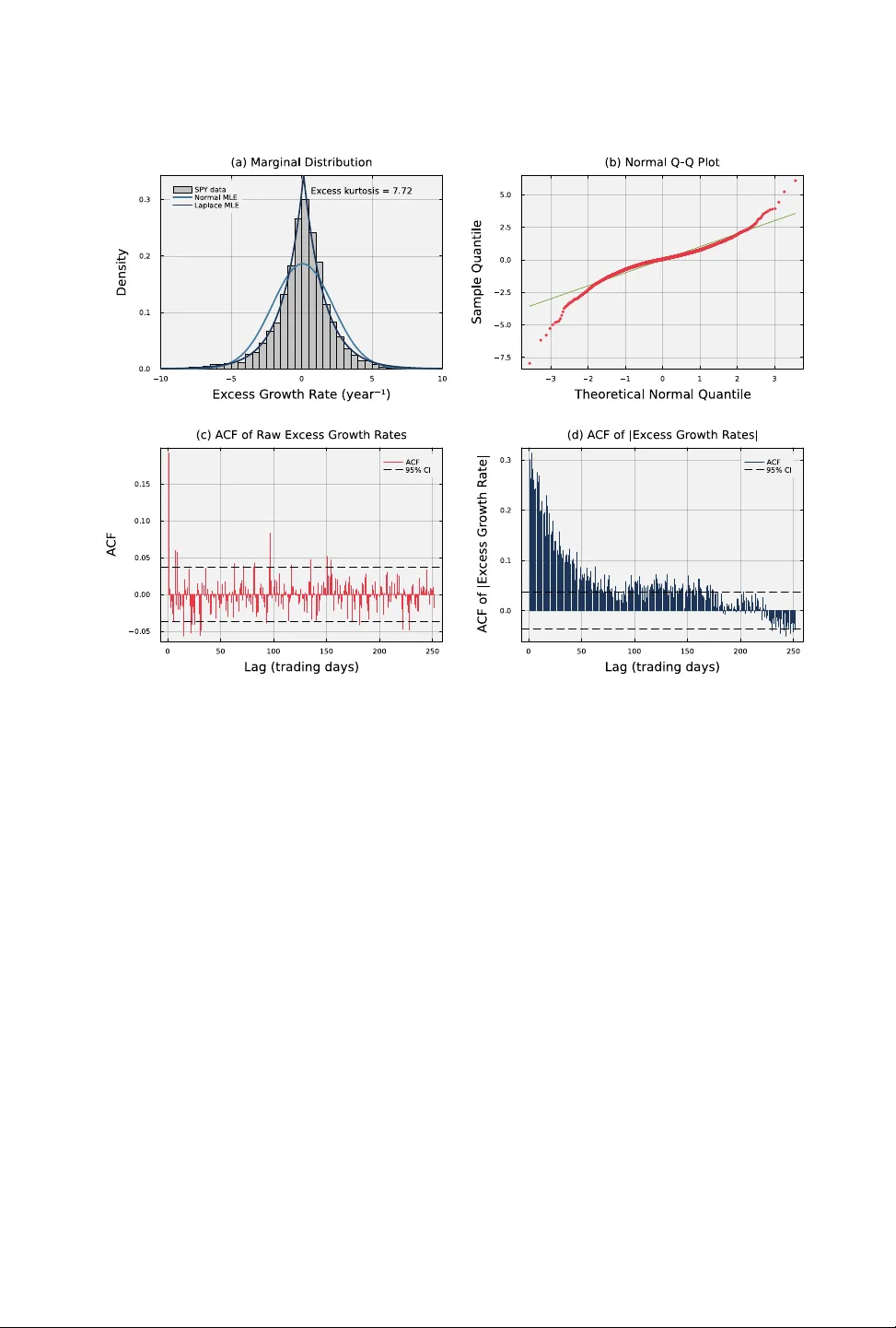
Hybrid Hidden Markov Model for Modeling Equity Excess Growth Rate Dynamics: A Discrete-State Appr oach with Jump-Diusion ABDULRAHMAN ALSW AID AN, Cornell University, USA JEFFREY V ARNER, Cornell University, USA Generating synthetic nancial time series that preserve the statistical properties of real market data is essential for stress testing, risk model validation, and scenario design, yet existing approaches, from parametric models to deep generative networks, struggle to simultaneously reproduce the heavy-tailed distributions, negligible linear autocorrelation, and persistent volatility clustering that characterize empirical equity data. W e propose a hybrid hidden Markov framework that discretizes continuous excess growth rates into Laplace quantile-dened market states and augments the regime-switching process with a Poisson-driven jump-duration mechanism to enforce realistic tail-state dwell times. Parameters are estimated by direct transition counting, avoiding the Baum- W elch EM algorithm entirely . W e evaluate synthetic data quality using three complementary metrics: Kolmogoro v-Smirnov and Anderson-Darling goodness-of-t pass rates for distributional delity , and A CF mean absolute error for temporal structure pr eservation. Applied to ten years of SPY data across 1,000 simulated paths, the framework achie ves KS and AD pass rates e xceeding 97% and 91% in-sample and 94% out-of-sample (full calendar year 2025), partially reproducing the ARCH eect that standard regime-switching models miss. No single mo del dominates all quality dimensions: GARCH(1,1) reproduces volatility clustering more accurately but fails distributional tests (5.5% KS pass rate), while the standard HMM without jumps achieves higher distributional delity but cannot generate persistent high-v olatility regimes. The proposed hybrid framew ork oers the b est joint quality prole across distributional, temp oral, and tail-co verage metrics among the parametric models evaluated. A Single-Index Model extension propagates the SPY factor path to a 424-asset universe, enabling scalable correlated synthetic path generation while preserving cross-sectional correlation structure. Additional K ey W ords and Phrases: Synthetic Data Quality , Time Series Generation, Hidden Markov Model, Jump-Diusion, V olatility Clustering, Regime-Switching, Stylized Facts, Distributional Fidelity 1 Introduction Generating synthetic nancial time series that faithfully preserve the statistical properties of real market data is a central challenge in quantitative nance and data quality r esearch. High-delity synthetic data are essential for stress testing risk models against plausible but unobserved market scenarios, validating portfolio optimization algorithms, and augmenting limited training sets for machine learning pip elines [ 3 , 33 ]. Y et the quality requirements for nancial synthetic data are unusually demanding: empirical equity excess growth rates exhibit three well-documented statistical regularities, namely heavy-tailed (leptokurtic) distributions, negligible linear autocorrelation in raw returns, and persistent volatility clustering, that any generative framew ork must simultaneously reproduce to be considered statistically faithful [ 15 , 41 , 52 ]. These domain-specic quality criteria, often called stylized facts , ser ve as the benchmark against which the delity of synthetic nancial data must be evaluated. Existing generative appr oaches address these quality requirements from dierent angles but each falls short on at least one dimension. GARCH-family models [ 9 , 21 ] capture conditional variance dynamics but do not explicitly represent discrete market regimes or sudden jumps in volatility . Stochastic-volatility and jump-diusion models [ 31 , 42 ] enrich tail behavior but lack a mechanism for volatility persistence after jumps. Deep generative models, including recurrent neural networks A uthors’ Contact Information: Abdulrahman Alswaidan, Cornell University, Robert Frederick Smith School of Chemical and Biomolecular Engineering, Ithaca, N Y, USA; Jerey V arner, Cornell University, Robert Frederick Smith School of Chemical and Biomolecular Engineering, Ithaca, N Y, USA, jdv27@cornell.edu. 2 Abdulrahman Alswaidan and Jerey V arner [ 26 , 32 ] and generative adv ersarial networks [ 38 , 53 , 55 ], can learn complex distributions from data but struggle to reproduce temporal dependence structures, particularly volatility clustering, unless the network architecture is specically designed to capture them [ 52 ]. Hidden Markov models (HMMs) and related regime-switching frame works oer a probabilistic structure for non-stationary market behavior through latent state dynamics [ 44 ], yet standard HMM sp ecications fail to generate persistent high-volatility regimes, leading to ov erly rapid rev ersion following extr eme events and poor temporal quality in the synthetic output [ 10 , 46 ]. Bridging this gap requires a generative framework that preserves b oth distributional delity and temp oral structure while remaining computationally scalable. W e address this challenge by dev eloping a hybrid HMM framework that discretizes continuous excess gr owth rates into quantile-based r egimes and augments the resulting Markov process with a two-parameter Poisson jump-duration mechanism that forces the model to dwell in high-volatility tail states for empirically realistic durations, connecting gradual price evolution with sudden large moves identied by jump-detection methods [ 4 ]. By partitioning excess growth rates into quantile-dened states via a Laplace cumulative distribution function, we enable direct frequentist counting of regime transitions, bypassing the iterative Baum- W elch algorithm (and its sensitivity to starting values) entirely , making the framework scalable to a 424-asset synthetic data pipeline. W e evaluate synthetic data quality using ve complementary metrics: Kolmogor ov-Smirnov (KS) and Anderson-Darling (AD ) pass rates for distributional delity , W asserstein-1 and Hellinger distances for ee ct-size quantication, and autocorrelation function mean absolute error (A CF-MAE) for temporal structure preservation, all reported with standard errors. Using ten years of SPY data (2014–2024) for training and 249 trading days (full calendar year 2025) for out-of-sample testing, we demonstrate KS and AD pass rates of 97.6% and 91.3% in-sample and 94.4% and 95.1% out-of-sample across 1,000 simulated paths, with volatility clustering preserved in both windows. A Single-Index Model factor extension [ 48 ] propagates the univariate SPY engine to the full 424-asset universe in a single generative pass, preserving cross-sectional correlation structure . W e nd that the jump- duration extension substantially improv es the reproduction of persistent high-volatility r egimes relative to standard regime-switching models, though the improvement is partial: approximately 24% of simulated paths contain jump episodes, shifting the ensemble ACF towar d the empirical prole without fully matching it. The framework does not dominate all quality dimensions; GARCH(1,1) achieves lower A CF error , and the standard HMM without jumps attains higher distributional pass rates. The contribution is a balance d quality prole that avoids the severe failures each alternative exhibits on its weakest dimension. 2 Related W ork Research on repr oducing the canonical stylized facts of nancial markets divides into tw o broad paradigms: bottom-up agent-based mo dels, which derive return dynamics from the simulate d interaction of heterogeneous agents, and top-down data-driven models, which t statistical struc- tures directly to observed return series. In the b ottom-up tradition, stylized facts emerge from collective behavior rather than b eing assumed. Lux and Marchesi [ 40 ] showed that a two-type fundamentalist-chartist population reproduces heavy tails and volatility clustering as emergent properties, Cont and Bouchaud [ 16 ] demonstrated that a simple random-graph herding structure alone is sucient to generate fat-tailed r eturn distributions, and Chen, T an, and Zheng [ 12 ] sho wed that multi-level herding simultaneously r eproduces sector structure and volatility clustering. The minority game of Challet and Zhang [ 11 ] introduced the paradigm of b ounded-rational agents competing via strategic coordination, a framework subsequently shown to produce non-Gaussian uctuations, and Farmer and Joshi [ 25 ] demonstrated that standard trading strategies simultane- ously deployed by many agents endogenously generate volatility clustering and excess ku rtosis Hybrid Hidden Markov Model for Modeling Equity Excess Growth Rate Dynamics: A Discrete-State Approach with Jump-Diusion 3 Fig. 1. Empirical stylized facts of SPY daily excess growth rates (2014–2024). Panel (a) shows the leptokurtic marginal distribution; the Laplace fit substantially outp erforms the Gaussian. Panel (b) confirms heavy tails via a normal Q-Q plot. Panels ( c) and (d) contrast the near-zero autocorrelation of raw r eturns (consistent with the eicient markets hypothesis) against the persistent autocorrelation of absolute returns, motivating the jump-duration extension. without any e xogenous noise assumption. LeBaron [ 39 ] surveys this class of models systematically; Arthur [ 2 ] provides a recent synthesis arguing that heterogeneous agent interactions give rise to phenomena inaccessible to e quilibrium the ory , and Farmer [ 24 ] demonstrates that quantitative ABMs can produce time-series predictions competitive with mainstr eam macroeconomic models. While mechanistically compelling, agent-base d models can b e challenging to calibrate directly to a specic asset’s return history and can be computationally demanding to deploy as practical syn- thetic data generators. T op-down models take the complementary approach: rather than explaining the origins of stylized facts, they specify statistical structures that match ho w those facts appear in data. GARCH, jump-diusion processes, HMMs, and deep generative ar chitectures all belong to this family; the subsections below survey each in turn, as they form the direct context for the present work. 2.1 Stylized facts and the limitations of parametric models The quantitative study of nancial market dynamics has been shaped by a tension b etween tractable theoretical frameworks and the empirical complexity of observed data. The Black-Scholes-Merton option pricing model [ 8 ] and the geometric Brownian motion (GBM) paradigm embe dded within it 4 Ab dulrahman Alswaidan and Jerey V arner assume that log-returns are independently and identically distributed Gaussian random variables, producing asset prices that move smoothly (no sudden jumps) with xed-size random uctuations and thin tails that assign negligible probability to extreme moves. These properties carry well- known practical advantages: closed-form option prices, simple portfolio variance calculations, and minimal data requirements. How ever , the Gaussian diusion paradigm conicts with a br oad set of empirical regularities documented well before the model’s widespread adoption. Mandelbrot [ 41 ] demonstrated that speculative price changes exhibit heavy tails far beyond Gaussian predictions, a property long characterized in statistics as leptokurtosis . Fama [ 22 ] review ed evidence that raw return series display negligible linear autocorrelation, consistent with the ecient markets hypoth- esis. Y et Schwert [ 47 ] and others documented that the magnitude of returns e xhibits substantial positive auto correlation de caying slowly over time: large price changes tend to be followed by large changes regardless of sign, a pattern referred to as v olatility clustering . Cont [ 15 ] provides a systematic review conrming these regularities across asset classes, geographic markets, and sampling frequencies. Collectively , leptokurtosis, the absence of return predictability , and volatility clustering dene the benchmark against which any mo del of market dynamics must be evaluated. The most inuential class of mo dels designed to address volatility clustering within the Gaussian framework is the autoregressive conditional heteroscedasticity (ARCH) family introduced by Engle [ 21 ], generalized by Bollerslev [ 9 ] to the GARCH(p,q) specication in which the conditional variance depends on both past squared residuals and past conditional variances. GARCH models are parsimonious and widely used, but they hav e well-documented limitations. Heavy tails must be injecte d by cho osing a fat-tailed noise distribution (e.g., Student-t); the model itself do es not produce them. There is no r epresentation of discrete market regimes or sudden jumps. V olatility persistence is controlled by a single decay parameter , so the mo del cannot distinguish between a calm market that slowly heats up and a sudden crash that lingers [ 18 ]. Stochastic volatility models [ 31 , 51 ] model volatility as a hidden quantity that ev olves randomly ov er time, addr essing some of these shortcomings, but require computationally intensive estimation and their parameters do not directly correspond to observable market states. An alternative approach to modeling fat tails and discontinuous price b ehavior is the explicit introduction of Poisson-driven jumps into the asset price process. Merton [ 42 ] added a compound Poisson jump component to GBM, producing a Gaussian-mixture marginal distribution that directly addresses leptokurtosis, and Kou [ 37 ] extended this framework with asymmetric jump sizes to captur e the empirical pattern that crashes tend to be sharper than rallies. Jump-diusion models are particularly relevant in equity markets, where macroeconomic announcements, earnings surprises, and geopolitical events generate discrete large-magnitude price movements [ 4 ]. Howev er , in their standard form, jump-diusion models do not provide a mechanism for volatility persistence: the p ost-jump volatility immediately returns to its baseline level, absent a separate stochastic volatility component. 2.2 Hidden Markov models and regime-switching Hidden Markov models (HMMs) provide a probabilistic framew ork for non-stationary time series in which the obser ved data are generated by a process that switches among a discrete set of latent states according to Markov dynamics. The Baum- W elch expectation-maximization algorithm for maximum-likelihood estimation of emission and transition parameters was introduced by Baum, Petrie, Soules, and W eiss [ 5 ]; Rabiner and Juang [ 44 ] provided the inuential tutorial that brought HMMs to widespread attention in engineering and applie d science. Hamilton [ 29 ] applied the regime-switching HMM to macroeconomic time series, demonstrating that U.S. GNP growth is well described by a two-state model with distinct expansion and recession regimes, establishing the template for latent-state modeling of nancial time series. The identication of time-varying Hybrid Hidden Markov Model for Modeling Equity Excess Growth Rate Dynamics: A Discrete-State Approach with Jump-Diusion 5 market regimes has since become a central application of HMMs in nance, with uses ranging from stock return modeling and volatility forecasting [ 45 ] to stock trading strategies [ 43 ]. Rydén, T eräsvirta, and Åsbrink [ 46 ] pro vided an inuential systematic evaluation of HMM specications against the stylized facts of daily return series, showing that simple Gaussian- emission HMMs with a small number of states could reproduce leptokurtosis and the absence of return autocorrelation, but failed to generate the obser ved volatility clustering; the A CF of absolute returns under standard HMMs de cayed far too rapidly relative to empirical data. This diagnostic limitation identied the core structural gap that the present study addresses. Bulla and Bulla [ 10 ] advance d this line of inquiry by considering hidden semi-Markov mo dels, in which the time spent in each state can follow a exible distribution rather than the simple memoryless (geometric) de cay of standard Markov chains, and showed that this extension substantially improves the reproduction of volatility clustering by allo wing the model to remain in high-volatility states for realistic durations. A persistent practical limitation of both standar d and semi-Markov HMM approaches is the computational burden of maximum-likelihood estimation via the EM algorithm, particularly when the number of states is large or the asset universe is broad: the Baum- W elch procedure requires iterative for ward-backward passes and may converge to local maxima depending on initialization. The present study addresses this limitation by replacing EM with direct frequentist counting of transitions between quantile-dened states, an approach that is computationally trivial and free of initialization sensitivity . 2.3 Synthetic data generation and deep generative models The generation of synthetic nancial time series has attracted increasing attention both as a prac- tical tool for augmenting limited data, testing risk models, and str ess testing portfolios, and as a benchmark for evaluating generative model quality . Assefa et al. [ 3 ] survey the opportunities, chal- lenges, and pitfalls of synthetic data generation in nance, noting that stylized-facts reproduction is the primary criterion for evaluating statistical quality and that naive generative approaches tend to fail on at least one of the three cor e stylized facts. The rise of generative adversarial netw orks (GANs) prompted several investigations into whether deep learning architectures could learn these properties from data. T akahashi, Chen, and T anaka-Ishii [ 53 ] showed that standard GAN architectures produce synthetic return sequences that visually r esemble nancial time series but fail to reproduce A CF structure precisely; K won and Lee [ 38 ] provided a careful evaluation against the stylized-facts checklist, nding that while GANs match marginal distributions reasonably well, capturing temporal dependence structures, particularly volatility clustering, r emains challenging unless the architecture is specically designed to learn them. Foundation mo dels for Markov jump processes [ 6 ] oer a complementar y p erspective in which large-scale pretrained inference networks can be applied to new process instances without retraining, but their application to nancial time series generation remains an open research direction. Against this backdrop, the hybrid HMM framework of the present study occupies a distinct position: it is explicitly designed around the structural properties known to generate stylized facts, uses an interpretable discrete-state representation that can b e audited and stress-tested, and achieves strong statistical delity with minimal computational overhead. The empirical estimation proce dure avoids the training instability and data r equirements of deep generative models, while the jump- duration mechanism provides a principled solution to the v olatility-clustering limitation of standar d HMMs. These properties make the frame work particularly well-suited for risk management and stress-testing pipelines, where interpretability and computational repr oducibility are as important as statistical delity . 6 Abdulrahman Alswaidan and Jerey V arner 2.4 Factor models and multi-asset extensions Modeling the joint dynamics of large asset universes requires a framework for managing cross- sectional dependence. The Single-Index Model (SIM) of Sharpe [ 48 ] provides the canonical linear factor decomp osition: each asset’s excess return is decomposed into a common market factor component and an idiosyncratic residual, drastically r educing the number of parameters needed compared with a full multivariate model. The SIM remains foundational in portfolio construction and risk management despite the availability of richer multi-factor models such as Fama-Fr ench [ 23 ], b ecause its simplicity enables transparent attribution and scalable computation. Existing HMM- based work in nance has b een predominantly univariate, focusing on single-asset or single-index regime identication. Applications to individual equities [ 43 ], volatility modeling [ 45 ], and macro time series [ 29 , 34 ] colle ctively demonstrate the utility of latent state representations but leav e op en the question of how HMM-derived generative models can be extended to large cross-sections of assets in a computationally tractable way . Mixture hidden Markov models [ 17 ] oer a partial solution by allowing multiple assets to share a common latent state structure, but estimating such models jointly across hundreds of assets is computationally demanding. An alternative approach to multi- asset dependence modeling uses copulas, which separate the spe cication of marginal distributions from the dependence structure [ 13 , 20 ]. Copula-based generators can capture nonlinear and tail dependence that linear factor models miss, and they have been applied extensively in credit risk and portfolio simulation. Howe ver , copula estimation becomes computationally demanding in high dimensions, and the choice of copula family introduces additional mo del selection complexity . The present study addresses the multi-asset challenge through a complementar y r oute by combining the univariate HMM framework with the SIM factor decomposition: the hybrid HMM is estimate d on the SPY index, which serves as the market-factor generator , and asset-level paths are reconstructed via the linear SIM projection. This construction exploits the fact that most of the shared volatility clustering across equities is driven by the broad market, yielding a scalable generative pipeline for a 424-asset universe that inherits the stylized-facts delity of the HMM without requiring joint estimation of a high-dimensional model. Hybrid Hidden Markov Model for Modeling Equity Excess Growth Rate Dynamics: A Discrete-State Approach with Jump-Diusion 7 3 Methods Data. The empirical foundation of this study was a dataset comp osed of 424 United States-liste d equities and exchange-traded funds spanning 10 years (2014-2024). A pip eline was de veloped to support the automated construction of excess growth rate models for any ticker within this dataset, allowing for batch simulation and stress testing acr oss market sectors. T o validate the performance of this pipeline, we focuse d our analysis on the single-asset SPY , which tracke d the Standard & Poor’s (S&P) 500 index. The data included daily open, high, low , and close prices along with volume-weighted average price metrics (VW AP). For training purposes, the rst 2,766 obser vations constituted the in-sample dataset, spanning from January 3, 2014, to December 31, 2024. A subsequent 249 trading days, from Januar y 2 to Decemb er 31, 2025, were reserved for out-of-sample testing to assess model generalizability . Excess growth rate calculation. W e compute d the excess growth rate 𝐺 𝑖 , 𝑗 for ticker 𝑖 between time perio d 𝑗 − 1 → 𝑗 for a given equity price series 𝑃 𝑖 , 𝑗 (units: dollars per share (USD/share)). T o measure how much each stock’s growth exceeded a risk-free baseline, we dened the excess gr owth rate as: 𝐺 𝑖 , 𝑗 ≡  1 Δ 𝑡  · ln  𝑃 𝑖 , 𝑗 𝑃 𝑖 , 𝑗 − 1  − 𝑟 𝑓 (1) where Δ 𝑡 represented the time step set to 1 / 252 for daily data (units: years), and 𝑟 𝑓 denoted the constant continuously compounded risk-free rate (units: y ear − 1 ) derived from Separate Trading of Registered Interest and Principal of Securities (STRIPS) bond yields observed on September 10, 2025. Unlike a simple return, the excess growth rate has units of inverse time (year − 1 ) and directly quanties the premium earned above a continuously compounded risk-free benchmark; log growth rates are also time-additiv e, making them consistent with a continuous compounding framework. While 𝑟 𝑓 varied dynamically over the sample period, we use d a constant proxy to isolate the volatility patterns in the data without adding noise from interest rate mo vements. Discrete hidden Markov model. W e dened the hidden Markov model using the tuple M = ( S , O , T , E , ¯ 𝜋 ) [ 44 ]. The hidden state 𝑆 𝑡 ∈ S = { 1 , . . . , 𝑁 } represented market mood regimes and was dened by quantile bins of a tted cumulative distribution function ( CDF) for the e xcess growth rate series. The observation space O ⊂ R consisted of continuous excess growth rate values, the transition matrix T governed regime-to-regime dynamics, the emission mo del E was parameterized by state-conditional Student-t distributions, and ¯ 𝜋 denoted the stationary distribution. The state-conditional obser vation model specied that the excess growth rate, given hidden state 𝑘 , followed a location-scale Student-t distribution with 𝜈 = 5 degrees of freedom: 𝐺 𝑡 | 𝑆 𝑡 = 𝑘 ∼ 𝜇 𝑘 + 𝜎 𝑘 · 𝑡 𝜈 , 𝜈 = 5 . (2) T o map obser vations to hidden states during estimation, we dened quantile b oundaries 𝑄 𝑘 = 𝐹 − 1 𝐿 ( 𝑘 / 𝑁 ; 𝜇 𝐿 , 𝑏 𝐿 ) for 𝑘 ∈ { 1 , . . . , 𝑁 − 1 } , with 𝑄 0 = −∞ and 𝑄 𝑁 = +∞ so that the partition cov ers the full support of the distribution. An obser vation was assigned to state 𝑘 when 𝑄 𝑘 − 1 < 𝐺 𝑡 ≤ 𝑄 𝑘 . The Laplace distribution was chosen for state partitioning rather than for emission modeling. Its sharper peak at the mean better matched the concentration of small price mov ements observed in the SPY dataset [ 15 , 36 , 41 , 54 ], and its closed-form quantile function supported the 424-ticker pipeline without iterative numerical optimization [ 7 ]. The quantile boundaries were derived from a parametric Laplace t and therefor e did not enforce equal counts per bin in the historical data; 8 Abdulrahman Alswaidan and Jerey V arner 1 2 · · · 𝑘 · · · 𝑁 − 1 𝑁 𝜇 𝑘 + 𝜎 𝑘 · 𝑡 5 emission Poisson clock prob. 𝜖 jump triggered 𝐾 ∼ Pois ( 𝜆 ) forced steps 𝐾 ∼ Pois ( 𝜆 ) forced steps S − (bottom tail) S + (top tail) state index prob. 1 − 𝜖 Fig. 2. Architecture of the Hybrid Hidden Markov Model with Jump-Diusion (HMM- WJ). At each step the chain transitions according to the empirical transition matrix T (probability 1 − 𝜖 , thin bidirectional arrows) or enters a Poisson jump episode (probability 𝜖 , dashed upward arrow to the Poisson clock). During a jump episode the active state is forced to the boom tail set S − (red, lowest-valued states) or the top tail set S + (blue, highest-valued states) for 𝐾 ∼ Poisson ( 𝜆 ) consecutive steps before normal Markovian evolution resumes. Small bell curves ab ove each state depict the state-conditional lo cation-scale Student-t ( 𝜈 = 5 ) emission distribution. T ail sets are defined as the 𝑁 tail lowest- and highest-quantile states under the Laplace quantile partition. instead, they pr ovided a partition of the distribution that preserved tail shape. By using the Laplace distribution to dene the bins, the model establishe d a baseline characterization of the return distribution’s shap e b efore the transition dynamics and jump me chanism were layered on top [ 37 ]. The emission distribution within each state, however , was a location-scale Student-t with 𝜈 = 5 degrees of freedom, chosen b ecause its heavier tails relative to the Normal distribution better reproduced the obser ved excess kurtosis of the growth rate series (a sensitivity analysis over 𝜈 ∈ { 3 , 4 , 5 , 6 , 7 , 8 , 10 , 15 , 30 , ∞ } identied 𝜈 = 5 as the value that minimized the kurtosis gap without degrading distributional delity; 𝜈 = ∞ recovers the Normal baseline). W e estimated the transition matrix T through direct frequentist counting rather than iterative optimization. This approach dier ed from the traditional expectation-maximization (EM) algorithm used for parameter estimation in Gaussian mixture and hidden Markov models [ 7 ]. Howev er , the discrete state assignments allow ed for straightforward counting of observed transitions between regimes, making the approach both conceptually simple and free of initialization sensitivity . A consequence of direct counting was that empirical transition matrices often had low probabilities for exiting central states into tail states, which caused models to lose the ee ct of volatility clustering too quickly [ 10 ]. W e corrected this by adding jump parameters 𝜖 , representing the probability of a jump event, and 𝜆 , representing the mean duration, along with a tail-state selection rule. T ail-states were dened as S 𝑏𝑜 𝑡 𝑡 𝑜𝑚 = { 1 , . . . , 𝑁 𝑡 𝑎𝑖𝑙 } and S 𝑡 𝑜 𝑝 = { 𝑁 − 𝑁 𝑡 𝑎𝑖𝑙 + 1 , . . . , 𝑁 } , where 𝑁 𝑡 𝑎𝑖𝑙 was user-congurable. If a jump was triggered, the jump-duration 𝐾 was sampled from a Poisson distribution such that 𝐾 ∼ Poisson ( 𝜆 ) , which was standard for modeling independent events in xed intervals [ 27 ]. During these 𝐾 steps, the standard Markovian transitions wer e overridden to target tail-states, with a user-congurable bias 𝑝 𝑛𝑒𝑔 (default 0.52) that fav ored negative-tail states to reproduce gain/loss asymmetry . Hybrid Hidden Markov Model for Modeling Equity Excess Growth Rate Dynamics: A Discrete-State Approach with Jump-Diusion 9 T o characterize the excess growth rates within each regime, we parameterized the emission model with lo cation-scale Student-t distributions 𝜇 𝑘 + 𝜎 𝑘 · 𝑡 5 , where 𝜇 𝑘 and 𝜎 𝑘 were the sample mean and standard deviation of observations assigne d to state 𝑘 . During simulation, when the model was in state 𝑘 , the continuous excess growth rate ( ˆ 𝐺 𝑡 ) was sampled from the corresponding local distribution. This hybrid approach ensured that the model captured sudden large price moves while keeping smooth variation within each regime [ 37 ]. The tted Laplace CDF closely matched the empirical CDF for SPY , and the empirical transition matrix exhibited a dominant near-diagonal band reecting short-range regime persistence (Figure S1 , Online Appendix S1). Critically , under pure Markovian dynamics the model exited extreme (tail) states after only 1–2 steps on average, far shorter than the multi-week v olatile episodes observed in real markets. This rapid r eversion was the core limitation that motivated the jump-duration extension. Growth rate generation. The basic sampling procedure for the HMM (without jumps) proceeded as follows. The stationary distribution ¯ 𝜋 , r epresenting the long-run probability of occupying each regime, satises the balance equation ¯ 𝜋 = ¯ 𝜋 T and was estimated numerically by raising the transition matrix to a large p ower ( T 50 ) [ 28 , 30 ]. An initial hidden state was drawn from 𝑋 0 ∼ ¯ 𝜋 , then for each subsequent step 𝑛 = 1 , . . . , 𝑇 : (i) the next hidden state was sample d from the transition row 𝑋 𝑛 ∼ T 𝑋 𝑛 − 1 , · , and (ii) an observation was sampled from the emission distribution 𝑂 𝑛 ∼ E 𝑋 𝑛 . This produced a sequence of hidden states { 𝑋 1 , . . . , 𝑋 𝑇 } and corresponding obser vations { 𝑂 1 , . . . , 𝑂 𝑇 } . Hyperparameter optimization via grid search. T o identify the optimal jump probability ( 𝜖 ) and mean jump duration ( 𝜆 ) [ 37 , 42 ], w e implemented a multi-objective grid search that minimized the discrepancy between historical and simulate d market signatures. The error function targeted two stylized facts [ 15 , 46 ]: volatility clustering, measured as the sum of squared errors between the observed and simulated autocorrelation function (A CF) of absolute excess growth rates [ 47 ] up to a lag of 𝐿 = 252 trading days (approximately one trading year); and leptokurtosis, captur ed by a penalty term on the global kurtosis [ 41 ]. W e dened the obje ctive function 𝐽 ( 𝜖 , 𝜆 ) as: 𝐽 ( 𝜖 , 𝜆 ) = 𝐿  𝜏 = 1  A CF 𝑜𝑏 𝑠 ( 𝜏 ) − A CF 𝑠𝑖 𝑚 ( 𝜏 )  2 + 𝑤 𝐾  𝐾 𝑜𝑏 𝑠 − 𝐾 𝑠𝑖 𝑚  2 (3) where A CF 𝑜𝑏 𝑠 ( 𝜏 ) and 𝐾 𝑜𝑏 𝑠 represented the empirical absolute growth autocorrelation at lag 𝜏 and the global kurtosis, respectively . The simulated equivalents, A CF 𝑠𝑖 𝑚 ( 𝜏 ) and 𝐾 𝑠𝑖 𝑚 , were av eraged across 200 independent synthetic paths of 2,766 trading days p er grid point [ 27 ]. W e set the kurtosis penalty weight to 𝑤 𝐾 = 0 . 20 to balance tail behavior against the temporal ACF term. The grid search explored 𝜖 values from 10 − 4 to 2 . 5 × 10 − 2 and 𝜆 values from 10 to 160 . The full computational procedure is detailed in Algorithm 4 . Statistical validation metrics T o assess whether synthetic paths were statistically consistent with empirical data, we applied two nonparametric goodness-of-t tests to the marginal distributions of simulated excess growth rate sequences. For each of the 1,000 simulated paths, the empirical cumulative distribution function (CDF) of the simulated sequence was compared against the empirical CDF of the historical in-sample or out-of-sample observations. 10 Abdulrahman Alswaidan and Jerey V arner The Kolmogor ov-Smirnov (KS) statistic is dened as: 𝐷 𝐾 𝑆 = sup 𝑥 | 𝐹 𝑛 ( 𝑥 ) − 𝐹 𝑚 ( 𝑥 ) | (4) where 𝐹 𝑛 and 𝐹 𝑚 denote the empirical CDFs of the observed and simulated sequences of lengths 𝑛 and 𝑚 , respectively [ 35 , 49 ]. The null hypothesis of distributional equivalence is rejected at signicance level 𝛼 when 𝐷 𝐾 𝑆 exceeds the critical value 𝑐 ( 𝛼 )  ( 𝑛 + 𝑚 ) / ( 𝑛𝑚 ) . The Anderson-Darling ( AD) statistic places greater weight on the distributional tails than the KS test. The original one-sample form [ 1 ] measures deviation from a fully specied reference CDF 𝐹 0 : 𝐴 2 = − 𝑛 − 𝑛  𝑖 = 1 2 𝑖 − 1 𝑛  ln 𝐹 0 ( 𝑋 ( 𝑖 ) ) + ln  1 − 𝐹 0 ( 𝑋 ( 𝑛 + 1 − 𝑖 ) )   (5) where 𝑋 ( 1 ) ≤ · · · ≤ 𝑋 ( 𝑛 ) are the order statistics of the sample. In this study , we applie d the two- sample Anderson-Darling test, which r eplaces 𝐹 0 with the empirical CDF of the observed SPY series; critical values are obtained from the 𝑘 -sample variant of Anderson and Darling as implemented in the HypothesisT ests.jl library . The AD test is particularly suited for assessing tail-distributional delity , which is the primar y concern for risk management applications. W e reporte d the pass rate as the proportion of the 1,000 simulate d paths for which the null hypothesis of distributional e quivalence was not rejected at the 𝛼 = 0 . 05 signicance level. A pass rate above 95 percent indicated that the synthetic paths were, in aggregate, statistically indistinguishable from the historical data under that test. Pass rates were r eported separately for the in-sample and out-of-sample windows and for both mo del variants (HMM without jumps and the hybrid HMM with jumps). Both KS and AD tests assume i.i.d. observations; be cause volatility clustering induces positive autocorrelation in the tail-indicator process 1 ( 𝐺 𝑡 ≤ 𝑥 ) , the eective sample size is smaller than 𝑇 and reported p-values may b e slightly miscalibrated. The continuous distance metrics below are unaected by this assumption. Continuous distributional distance metrics Binary pass rates summarize distributional delity but discard information ab out the magnitude of any discrepancy . The W asserstein-1 distance ( 𝑊 1 ) and the Hellinger distance ( 𝐻 ) were computed alongside KS and AD to pr ovide continuous, eect-size measures that do not depend on sample size. The W asserstein-1 distance measures the minimum work required to transform one distribution into the other , where work is distance times probability mass moved. For two e qual-length empirical samples with order statistics 𝑥 ( 1 ) ≤ · · · ≤ 𝑥 ( 𝑇 ) and 𝑦 ( 1 ) ≤ · · · ≤ 𝑦 ( 𝑇 ) , the one-dimensional W asserstein-1 distance is: 𝑊 1 = 1 𝑇 𝑇  𝑖 = 1   𝑥 ( 𝑖 ) − 𝑦 ( 𝑖 )   (6) 𝑊 1 is expressed in the same units as the data (daily excess growth rates) and equals zero only when the empirical distributions are identical. Because it is computed from sorted order statistics, the temporal ordering of observations is irrelevant; smaller values indicate closer distributional agreement across the full quantile range. The Hellinger distance measures distributional overlap and is bounde d in [ 0 , 1 ] , with 𝐻 = 0 indi- cating identical distributions and 𝐻 = 1 indicating completely disjoint support. Given normalized histogram estimates { 𝑝 𝑘 } 𝐾 𝑘 = 1 and { 𝑞 𝑘 } 𝐾 𝑘 = 1 of the observed and simulate d marginal densities over a Hybrid Hidden Markov Model for Modeling Equity Excess Growth Rate Dynamics: A Discrete-State Approach with Jump-Diusion 11 common 𝐾 -bin grid: 𝐻 ( 𝑃 , 𝑄 ) = 1 √ 2 v u t 𝐾  𝑘 = 1  √ 𝑝 𝑘 − √ 𝑞 𝑘  2 (7) The bounded scale makes 𝐻 directly comparable across models and evaluation windows without rescaling. Histograms were constructed on the common support of observed and simulated samples using 𝐾 = 50 equal-width bins. Both 𝑊 1 and 𝐻 were computed path-by-path and averaged across the 1,000 paths; standard errors wer e estimated as std / √ 𝑛 paths . T emporal fidelity metric While KS and AD tests assess marginal distributional quality , they are insensitive to temporal dependence. T o measure how well a generator reproduced volatility clustering, we dene d the autocorrelation mean absolute error ( A CF-MAE) as: A CF-MAE = 1 𝐿 𝐿  𝜏 = 1    b 𝜌 obs | 𝐺 | ( 𝜏 ) − b 𝜌 sim | 𝐺 | ( 𝜏 )    (8) where b 𝜌 obs | 𝐺 | ( 𝜏 ) and b 𝜌 sim | 𝐺 | ( 𝜏 ) are the sample autocorrelations of the absolute excess gr owth rate series | 𝐺 𝑡 | at lag 𝜏 for the observed and simulated paths, respectively , and 𝐿 = 252 (one trading year ). An i.i.d. generator produces b 𝜌 sim | 𝐺 | ( 𝜏 ) ≈ 0 for all 𝜏 > 0 , so its A CF-MAE equals the mean level of the observed auto correlation function; lower values indicate better reproduction of empirical volatility persistence. Single-Index Factor Model extension The framework described above applied to any individual asset ticker within the 424-asset dataset. T o generalize synthetic path generation to a correlated multi-asset setting without tting a separate HMM for each asset, we exploited the linear factor structure of the Single-Index Model (SIM) [ 48 ]. The SIM expresses the excess gr owth rate of asset 𝑖 at time 𝑡 as: 𝐺 𝑖 ,𝑡 = 𝛼 𝑖 + 𝛽 𝑖 · 𝐺 SPY , 𝑡 + 𝜂 𝑖 ,𝑡 , 𝜂 𝑖 ,𝑡 i.i.d. ∼ N ( 0 , 𝜎 2 𝜂,𝑖 ) (9) where 𝐺 SPY , 𝑡 denotes the SPY excess growth rate at time 𝑡 , 𝛽 𝑖 measures the systematic sensitivity of asset 𝑖 to the index, 𝛼 𝑖 is the idiosyncratic drift, a nd 𝜂 𝑖 ,𝑡 is a zero-mean idiosyncratic sho ck assumed independent across assets and time. The parameters ( 𝛼 𝑖 , 𝛽 𝑖 , 𝜎 2 𝜂,𝑖 ) were estimated via ordinary least squares on the in-sample time series for each asset 𝑖 . Synthetic multi-asset paths were generated in three steps. First, the hybrid HMM produced a single synthetic SPY excess growth rate path { ˆ 𝐺 SPY , 𝑡 } 𝑇 𝑡 = 1 using the regime-switching and jump- duration mechanism describ ed above. Second, for each asset 𝑖 , an idiosyncratic shock sequence { ˆ 𝜂 𝑖 ,𝑡 } was drawn independently from N ( 0 , ˆ 𝜎 2 𝜂,𝑖 ) . Third, the synthetic excess growth rate for asset 𝑖 was recovered as: ˆ 𝐺 𝑖 ,𝑡 = ˆ 𝛼 𝑖 + ˆ 𝛽 𝑖 · ˆ 𝐺 SPY , 𝑡 + ˆ 𝜂 𝑖 ,𝑡 . (10) This construction preserved the cross-sectional correlation structure induced by the common factor while maintaining the regime-switching and jump-diusion dynamics of the index. The resulting 424-dimensional synthetic path could b e used for stress testing, p ortfolio risk assessment, and scenario generation across the full asset universe in a single generative pass, avoiding the curse of dimensionality that would accompany a full multivariate HMM. 12 Abdulrahman Alswaidan and Jerey V arner Algorithm 1 Hybrid jump-diusion simulation with p ersistent volatility Require: Model parameters T , ¯ 𝜋 , 𝜖 , 𝜆 , 𝑁 𝑡 𝑎𝑖 𝑙 , 𝑝 𝑛𝑒𝑔 , T otal Steps 𝑀 Ensure: Simulated state sequence 𝑆 1: 𝑀 1: Dene tail-states S 𝑏𝑜 𝑡 𝑡𝑜 𝑚 = { 1 , . . . , 𝑁 𝑡 𝑎𝑖 𝑙 } and S 𝑡 𝑜 𝑝 = { 𝑁 − 𝑁 𝑡 𝑎𝑖 𝑙 + 1 , . . . , 𝑁 } . 2: Sample initial state 𝑆 1 ∼ Categorical ( ¯ 𝜋 ) . 3: Set 𝑐 𝑜𝑢 𝑛𝑡 𝑒𝑟 ← 2 . 4: while 𝑐 𝑜𝑢 𝑛𝑡 𝑒𝑟 ≤ 𝑀 do 5: Sample 𝑢 ∼ Uniform ( 0 , 1 ) . 6: if 𝑢 < 𝜖 then 7: Sample jump-duration 𝐾 ∼ Poisson ( 𝜆 ) . 8: for 𝑗 = 1 to 𝐾 while 𝑐 𝑜 𝑢𝑛𝑡 𝑒 𝑟 ≤ 𝑀 do 9: Sample 𝑤 ∼ Uniform ( 0 , 1 ) . 10: if 𝑤 < 𝑝 𝑛𝑒𝑔 then 11: 𝑆 𝑐𝑜 𝑢𝑛𝑡 𝑒𝑟 ∼ Uniform ( S 𝑏𝑜 𝑡 𝑡𝑜 𝑚 ) {Bias toward negative-tail events} 12: else 13: 𝑆 𝑐𝑜 𝑢𝑛𝑡 𝑒𝑟 ∼ Uniform ( S 𝑡 𝑜 𝑝 ) 14: end if 15: 𝑐𝑜 𝑢 𝑛𝑡 𝑒𝑟 ← 𝑐 𝑜𝑢 𝑛𝑡 𝑒𝑟 + 1 . 16: end for 17: else 18: Sample 𝑆 𝑐𝑜 𝑢𝑛𝑡 𝑒𝑟 ∼ Categorical ( T 𝑆 𝑐𝑜 𝑢𝑛𝑡 𝑒𝑟 − 1 , : ) . 19: 𝑐𝑜 𝑢 𝑛𝑡 𝑒𝑟 ← 𝑐 𝑜𝑢 𝑛𝑡 𝑒𝑟 + 1 . 20: end if 21: end while 22: return 𝑆 1: 𝑀 Simulation algorithm Algorithm 1 details the core jump-diusion simulation pr ocedure; the remaining pipeline stages (model construction, state deco ding, and hyp erparameter grid search) are provided in Online Appendix S4. Hybrid Hidden Markov Model for Modeling Equity Excess Growth Rate Dynamics: A Discrete-State Approach with Jump-Diusion 13 T able 1. Descriptive statistics and stylized-facts tests for SPY daily e xcess growth rates. In-sample: 2014–2024 ( 𝑇 = 2 , 766 ); out-of-sample: 2025 ( 𝑇 = 249 ). Gaussian and Laplace columns sho w MLE fits to the in-sample data. JB = Jarque-Bera normality test. LB = Ljung-Box autocorrelation test at lag 20. ∗ denotes rejection at 𝛼 = 0 . 05 . Statistic IS Observed OoS Observed Gaussian Laplace Mean (annualized, %) 6.31 11.60 6.31 14.19 Std Dev (annualized, %) 214.50 220.62 214.46 205.93 Skewness − 0 . 753 − 1 . 093 0 0 Excess Kurtosis 7.715 6.867 0 3 JB normality test reject ∗ ( 𝑝 < 0 . 001 ) reject ∗ ( 𝑝 < 0 . 001 ) n/a n/a LB test on 𝐺 𝑡 (lag 20) reject ∗ ( 𝑝 < 0 . 001 ) reject ∗ ( 𝑝 = 0 . 019 ) n/a n/a LB test on | 𝐺 𝑡 | (lag 20) reject ∗ ( 𝑝 < 0 . 001 ) reject ∗ ( 𝑝 < 0 . 001 ) n/a n/a 4 Empirical Study 4.1 Descriptive statistics and stylized facts Descriptive statistics for the SPY daily excess growth rate series conrmed that the three canonical stylized facts were present in both the in-sample (2014–2024, 𝑇 = 2 , 766 ) and out-of-sample (2025, 𝑇 = 249 ) windows (T able 1 ). Excess kurtosis ( kurtosis minus 3, so that a Gaussian distribution has a value of zero) reached 7.7 (IS) and 6.9 (OoS), and the Jarque-Bera normality test was rejecte d ( 𝑝 < 0 . 001 ) in both windows, conrming leptokurtosis. The Ljung-Box test on | 𝐺 𝑡 | was rejected ( 𝑝 < 0 . 001 ) in b oth windows, conrming persistent volatility clustering. The Ljung-Box test on raw returns 𝐺 𝑡 was also formally rejected ( 𝑝 < 0 . 001 IS, 𝑝 = 0 . 019 OoS); while this indicates statistically detectable linear autocorrelation, the eect is small in magnitude at daily frequency and is consistent with the broad EMH literature, which documents that return predictability is weak rather than strictly absent [ 22 ]. Any faithful generative model must reproduce leptokurtosis, the ARCH eect, and the near-absence of large-magnitude return predictability simultaneously . 4.2 Jump hyperparameter optimization and state resolution A multi-objective grid search over 𝜖 ∈ [ 10 − 4 , 2 . 5 × 10 − 2 ] and 𝜆 ∈ [ 10 , 160 ] , with 200 simulated paths per grid point, identied the optimal values 𝜖 ∗ = 10 − 4 and 𝜆 ∗ = 100 (Figure S2 , Online Appendix S2). The optimal 𝜆 ∗ = 100 was an interior point of the 𝜆 grid, conrming that the mean jump duration was identiable from data; 𝜖 ∗ = 10 − 4 fell at the low er boundary of the 𝜖 grid, indicating that the data consistently preferred rarer tail-entry events over the range explored. At these optimal values, the A CF of | 𝐺 𝑡 | closely tracked the obser ved SPY ACF across lags 1–252, conrming that the jump mechanism partially reproduced the empirical ARCH eect. The primary analysis use d 𝑁 = 100 states, but a sensitivity study over 𝑁 ∈ { 30 , 60 , 90 , 100 , 150 , 200 } showed that the frame work was robust to the choice of state r esolution across a wide range (T a- ble T1 , Online App endix S3). KS and AD pass rates remained stable for b oth HMM-NJ ( ≥ 98.9% KS, ≥ 97.9% AD) and HMM- WJ ( ≥ 96.0% KS, ≥ 88.6% AD), while A CF-MAE for HMM- WJ improved slightly from 0.057 at 𝑁 = 30 to 0.049 at 𝑁 = 200 . State-occupancy diagnostics conrmed that every state at 𝑁 ≤ 200 contained at least 7 observations, ensuring ade quate statistical support per state under the Laplace e qual-probability partition. At 𝑁 = 350 , howev er , certain states were nev er visited in the historical record, leaving zero transition probabilities that prevented the model from reaching all states, which established a practical upper bound on state resolution. 14 Abdulrahman Alswaidan and Jerey V arner 4.3 In-sample distributional and temporal quality W e generated 1,000 synthetic paths of 2,766 trading days from each of eight generators and evaluated them against the observed SPY series using two-sample KS and AD tests at 𝛼 = 0 . 05 , along with the W asserstein-1 distance, Hellinger distance, kurtosis matching, A CF delity , novelty , diversity , and quantile coverage (T able 2 ). Baseline anchors. W e include d three non-structured baselines and one semi-Markov baseline to bracket the quality landscape. Bootstrap resampling of the training data served as a non-parametric upper bound: we observed 100.0% KS and 99.7% AD pass rates with 100% quantile coverage , but this generator simply recycled observed values and could not pr oduce genuinely new distributional structure (0 estimated parameters). The Gaussian i.i.d. baseline (MLE t) achieved 0.0% KS and 0.0% AD pass rates, which conrmed that a symmetric thin-tailed mo del was categorically inadequate for heav y-tailed equity returns. The Laplace i.i.d. baseline fared b etter at 44.0% (SE 1.6) KS and 43.3% (SE 1.6) AD , which sho wed that matching the tail decay rate alone recover ed roughly half the distributional quality; the remaining gap reected the regime-dependent variation that a single Laplace distribution could not capture . The hidden semi-Markov model (HSMM) baseline, implemented following Bulla and Bulla with 𝐾 = 8 Laplace quantile states, negative-binomial dwell-time distributions, and Student-t( 𝜈 = 5 ) emissions, achieved 82.0% (SE 1.2) KS and 42.5% (SE 1.6) AD in-sample. A sweep over 𝐾 ∈ { 3 , 4 , 5 , 6 , 8 } selected 𝐾 = 8 as the b est-performing conguration; at all 𝐾 values, the empirical dw ell times averaged only 1.1–1.8 steps per state, which meant the negative-binomial distributions collapsed to geometric (memor yless) behavior and the HSMM reduced to a standard coarse-state HMM. This conrme d that explicit dwell-time modeling alone could not reproduce the observed volatility clustering when state resolution was too coarse for accurate distributional matching, and too ne for meaningful dwell-time structur e. The GRU neural baseline, a 2-layer gated recurrent unit trained autoregressively on the IS series with a Gaussian output head (37,954 trainable parameters), exhibited the inverse failure mode: it achieved the second-lowest ACF-MAE of any model (0.036, behind only GARCH at 0.031) but catastrophically failed distributional tests (0.6% KS, 0.2% AD) with a W asserstein-1 distance of 0.421, worse than all mo dels except Gaussian. The GRU learned the temporal dynamics of returns eectively but suered from variance collapse: simulated standard deviation was 30% below the observed value, and excess kurtosis fell to 5.7 against an obser ved 7.7. This pattern, strong temporal delity paired with poor marginal t, is the mirror image of the HMM-NJ tradeo and illustrates the diculty of simultaneously capturing both quality dimensions with a single modeling paradigm. Distributional delity . W e evaluated KS/AD pass rates and kurtosis matching for the ve struc- tured models (T able 2 ). GARCH(1,1) achieved IS KS and AD pass rates of only 5.5% (SE 0.7) and 1.9% (SE 0.4), which indicated that the GARCH marginal distribution was systematically inconsistent with the observed data despite its well-known volatility clustering properties. The HSMM occupied a middle ground (82.0% KS, 42.5% AD ), outperforming GARCH and Laplace but falling well short of the HMM variants; its coarse 8-state partition could not capture the full shap e of the growth rate distribution, as reected by a simulated kurtosis of 4.8 against an obser ved 7.7 (38% gap) and only 68.7% quantile coverage. HMM-NJ achie ved 99.7% (SE 0.2) and 99.1% (SE 0.3), and HMM- WJ achieved 97.6% (SE 0.5) and 91.3% (SE 0.9). Both HMM variants adequately captured the observed heavy-tailed distribution, though HMM-WJ’s pass rates w ere 2–8 percentage points lower than HMM-NJ’s, a cost of the jump mechanism which occasionally distorted the marginal distribution by overweighting tail states during jump episodes. Simulated excess kurtosis told a complementar y story: the obser ved value was 7.7, GARCH overshot at 8.2 (SE 0.37) with high variance across paths, while HMM-NJ and HMM- WJ produced 8.1 (SE 0.14) and 7.6 (SE 0.14) respectively . The Hybrid Hidden Markov Model for Modeling Equity Excess Growth Rate Dynamics: A Discrete-State Approach with Jump-Diusion 15 Student-t( 𝜈 = 5 ) emissions closely matche d the observed kurtosis (within 2% for HMM- WJ), a substantial improvement ov er Normal emissions which underestimated kurtosis by approximately 29%; a sensitivity analysis over 𝜈 ∈ { 3 , . . . , 30 , ∞ } conrmed that 𝜈 = 5 minimized the kurtosis gap without degrading other metrics. Quantile coverage reinforced these ndings: Bo otstrap, HMM-NJ, and HMM- WJ all achieved 100% coverage of the 1st–99th empirical percentiles, while Gaussian covered only 13.1%, Laplace 37.4%, GARCH 29.3%, and HSMM 68.7%, which indicated systematic tail misspecication in all non-HMM parametric generators (Figure 3 , panel c). Continuous distributional distances. T o complement the binar y KS and AD pass rates with ee ct- size information that does not depend on sample size, we computed the W asserstein-1 distance 𝑊 1 and the Hellinger distance 𝐻 for each simulated path against the obser ved SPY series (T able 2 ). 𝑊 1 quanties the average absolute displacement b etween the sorte d empirical quantiles of the simulated and observed distributions (Eq. 6 ), expressed in units of daily excess growth rates; 𝐻 measures distributional overlap on a bounde d [ 0 , 1 ] scale (Eq. 7 ), where zero indicates identical distributions and one indicates disjoint support. In-sample , both metrics conrmed the ordering established by KS and AD: Bo otstrap achieved the lowest values ( 𝑊 1 = 0 . 062 , 𝐻 = 0 . 042 ), followed by HMM-NJ ( 𝑊 1 = 0 . 081 , 𝐻 = 0 . 073 ) and then HMM-WJ ( 𝑊 1 = 0 . 101 , 𝐻 = 0 . 075 ), with Laplace, GARCH, and Gaussian progressiv ely larger . HMM-NJ’s lower 𝑊 1 relative to HMM- WJ reected the same distributional cost of the jump mechanism observed in the pass rates: enforcing tail-state persistence improved temporal delity at the e xpense of marginal t. Out-of-sample, the continuous metrics revealed a pattern obscured by binary pass rates: GARCH’s 𝑊 1 increased sharply from 0.304 (IS) to 0.507 (OoS), making it the worst-performing model out-of-sample by a wide margin and worse even than the Gaussian baseline ( OoS 𝑊 1 = 0 . 452 ). This deterioration occurred despite GARCH recovering to an 80.3% KS pass rate out-of-sample, a r ecovery driv en by reduced test power at 𝑇 = 249 rather than genuine distributional delity . GARCH’s simulated kurtosis collapse d to 1.6 against an observed 6.9, a tail missp ecication that 𝑊 1 captured directly while the binary pass rate obscured it. By contrast, HMM-NJ and HMM- WJ maintained the lowest 𝑊 1 among parametric models both in-sample and out-of-sample (OoS 𝑊 1 = 0 . 258 and 0 . 282 respectively), with Hellinger distances clustering narrowly b etween 0.207 and 0.210, conrming robust generalization to the held-out window . T emporal delity . W e measured temp oral quality using the mean absolute error of A CF ( | 𝐺 𝑡 | ) over lags 1–252. Bootstrap, Gaussian, and Laplace all produced an A CF-MAE of 0.060, which was expected be cause i.i.d. draws destroy all temporal dependence by construction. GARCH achieved the lowest A CF-MAE (0.031, SE 0.001) be cause its variance equation was explicitly designed to match autocorrelation structure; however , this advantage came at the cost of distributional delity , a tradeo that the quality metrics exposed directly . HMM-NJ scored 0.059 (SE < 0.001), essentially indistinguishable from the i.i.d. oor , which conrmed that the standard transition matrix alone was structurally incapable of generating p ersistent volatility clustering (Figure 3 , panel b). The GRU achieved 0.036 (SE < 0.001), the second-lowest A CF-MAE overall, demonstrating that the recurrent architecture eectively captured short-range temporal dep endencies; however , this came at the cost of catastr ophic distributional failure (0.6% KS pass rate). HMM- WJ scored 0.052 (SE < 0.001), the only non-GARCH, non-neural mo del to reduce ACF-MAE meaningfully below the i.i.d. baseline, though the gap to GARCH remained substantial (0.052 vs. 0.031). The impro vement arose because approximately 24% of HMM- WJ paths contained at least one Poisson jump event that sustained A CF ( | 𝐺 𝑡 | ) decay across all lags, while the remaining 76% b ehaved identically to HMM-NJ. Importantly , the jump frequency is continuously tunable: incr easing 𝜖 produces more jump-containing paths and further reduces ACF-MAE, at the cost of degrading distributional delity . The grid search selected 𝜖 ∗ = 10 − 4 because this value minimized the joint objective over both 16 Abdulrahman Alswaidan and Jerey V arner Fig. 3. Head-to-head in-sample model comparison for SPY ( 𝑁 = 100 , 1,000 simulated paths). Panel (a): marginal density of excess gr owth rates with IS KS pass rates annotated. GARCH(1,1) fails the two-sample KS test on 95% of paths (pass rate 5.5%), indicating a systematic shape mismatch with the empirical distribution. Both HMM variants pass at rates ≥ 97% , confirming that the Student-t emission structure adequately captures the observed heav y tails. Out-of-sample, HMM- WJ maintains 94% KS pass rate, though HMM-NJ achieves a higher 97%; GARCH recovers partially (OoS 80%). Panel ( b): auto correlation function of absolute excess growth rates, A CF ( | 𝐺 𝑡 | ) , at lags 1–252 (shaded bands: 10th–90th percentile across paths). HMM-NJ is structurally incapable of producing persistent volatility clustering: without a jump mechanism the latent states are i.i.d. conditional on the Markov chain, so A CF ( | 𝐺 𝑡 | ) ≈ 0 for all lags b eyond one ( doed curve). HMM- WJ generates a mixture of two path families under the same model: approximately 76% of IS paths contain no Poisson jump and therefore behave identically to HMM-NJ (dashed curve, near zero); the remaining ∼ 24% of paths contain at least one jump event and sustain substantial A CF ( | 𝐺 𝑡 | ) decay across all lags (solid navy cur ve ± band). The jump frequency , and hence the fraction of the ensemble exhibiting slow ACF decay , is controlled by the tail-entry probability 𝜖 , making the volatility-clustering strength directly tunable. Panel ( c): tail Q-Q plot at the 0.1st–99.9th percentile region; HMM- WJ provides the closest mean quantile match in the extreme tails. temporal and distributional quality (Equation 3 ), meaning the 24% jump rate was the empirically optimal operating point for SPY , not a structural ceiling. The jump-duration mechanism was therefore the structural feature responsible for partially reproducing the ARCH eect, with its strength directly controlled by 𝜖 . Novelty , diversity , and parsimony . W e computed novelty (mean correlation distance to the ob- served series) and diversity (mean pairwise correlation distance among synthetic paths) to verify that the generators produced genuinely new , non-redundant scenarios. All seven models scored between 0.984 and 0.985 on b oth IS metrics, which conrmed that no generator memorized the training data and that synthetic paths were mutually independent. This uniformity was expected: all generators produced stochastic paths that were uncorr elated with any specic historical real- ization. Finally , HMM- WJ achieved the best joint distributional and temp oral quality among all parametric models with four scalar parameters requiring explicit estimation: the Laplace location 𝜇 𝐿 and scale 𝑏 𝐿 (MLE), and the jump hyperparameters 𝜖 and 𝜆 (grid search). The 𝑁 × 𝑁 transition matrix is a non-parametric empirical estimate obtained by dir ect counting and is therefor e not a free parameter in the modeling sense. This compares favorably in interpretability with GARCH (three scalar parameters: 𝜔 , 𝛼 , 𝛽 ) and Gaussian/Laplace baselines (two parameters each), though the transition matrix does add complexity that is not reected in the scalar parameter count. 1 The 𝑁 × 𝑁 transition matrix in HMM-NJ and HMM- WJ is computed by direct counting of observed state transitions; it is a sucient statistic of the data, not a tted parameter . The counts liste d here reect only the scalar parameters requiring estimation (MLE or grid search). Hybrid Hidden Markov Model for Modeling Equity Excess Growth Rate Dynamics: A Discrete-State Approach with Jump-Diusion 17 T able 2. In-sample and out-of-sample model comparison for SPY (1,000 simulated paths, significance lev el 𝛼 = 0 . 05 ). Bootstrap: i.i.d. resample of training data. Gaussian/Laplace: i.i.d. draws from MLE-fied distributions. GARCH: GARCH(1,1) estimated by quasi-maximum likelihood. GRU: 2-layer gated recurrent unit [ 14 ] with Gaussian output head (autoregr essive generation). HSMM: hidden semi-Markov model with 𝐾 = 8 Laplace quantile states, negative-binomial dw ell times, and Student-t( 𝜈 = 5 ) emissions [ 10 ]. HMM-NJ: hidden Markov model ( 𝑁 = 100 states) without jumps. HMM-WJ: hybrid model with Poisson jump-duration extension. A CF-MAE: mean absolute error of the A CF of | 𝐺 𝑡 | over lags 1–252. W asserstein-1: mean absolute dierence of sorted empirical quantiles (Eq. 6 ); units are daily excess growth rates. Hellinger: histogram-base d distributional overlap distance in [ 0 , 1 ] (Eq. 7 ); 𝐻 = 0 is identical, 𝐻 = 1 is disjoint. Novelty: mean correlation distance 1 − | 𝜌 | between each synthetic path and the observed series. Diversity: mean pairwise correlation distance among synthetic paths. Coverage: fraction of 99 empirical quantiles (1st–99th) falling within the [5th, 95th] percentile envelope of the corresponding synthetic quantiles. Standard errors in parentheses: binomial SE for pass rates, std / √ 𝑛 for kurtosis, novelty , W asserstein-1, and Hellinger , bootstrap SE ( 𝐵 = 500 ) for A CF-MAE, diversity , and coverage. Arr ows indicate preferr ed direction: ↑ higher is beer , ↓ lower is beer , ≈ closer to observed is beer . Metric Bootstrap Gaussian Laplace GARCH(1,1) GRU HSMM HMM-NJ HMM- WJ In-sample: 2,766 trading days (2014–2024) KS pass rate (%) ↑ 100.0 ( < 0.1) 0.0 ( < 0.1) 44.0 (1.6) 5.5 (0.7) 0.6 (0.2) 82.0 (1.2) 99.7 (0.2) 97.6 (0.5) AD pass rate (%) ↑ 99.7 (0.2) 0.0 ( < 0.1) 43.3 (1.6) 1.9 (0.4) 0.2 (0.1) 42.5 (1.6) 99.1 (0.3) 91.3 (0.9) Excess kurtosis (observed) 7.715 Excess kurtosis (simulated) ≈ 7.6 (0.08) − 0.0 ( < 0.01) 3.0 (0.02) 8.2 (0.37) 5.7 (0.16) 4.8 (0.08) 8.1 (0.14) 7.6 (0.14) ACF-MAE ↓ 0.060 ( < 0.001) 0.060 ( < 0.001) 0.060 ( < 0.001) 0.031 (0.001) 0.036 ( < 0.001) 0.059 ( < 0.001) 0.059 ( < 0.001) 0.052 ( < 0.001) Novelty ↑ 0.985 ( < 0.001) 0.984 ( < 0.001) 0.985 ( < 0.001) 0.985 ( < 0.001) 0.984 ( < 0.001) 0.985 ( < 0.001) 0.985 ( < 0.001) 0.984 ( < 0.001) Diversity ↑ 0.985 ( < 0.001) 0.985 ( < 0.001) 0.985 ( < 0.001) 0.985 ( < 0.001) 0.984 ( < 0.001) 0.985 ( < 0.001) 0.984 ( < 0.001) 0.984 ( < 0.001) Coverage (%) ↑ 100.0 ( < 0.1) 13.1 (0.1) 37.4 (1.5) 29.3 (1.4) 17.2 (0.5) 68.7 (1.1) 100.0 ( < 0.1) 100.0 ( < 0.1) W asserstein-1 ↓ 0.062 (0.001) 0.399 (0.001) 0.138 (0.001) 0.304 (0.006) 0.421 (0.003) 0.176 (0.001) 0.081 (0.001) 0.101 (0.001) Hellinger dist ↓ 0.042 ( < 0.001) 0.148 ( < 0.001) 0.072 ( < 0.001) 0.100 (0.001) 0.134 (0.001) 0.113 ( < 0.001) 0.073 ( < 0.001) 0.075 ( < 0.001) Out-of-sample: 249 trading days (2025) KS pass rate (%) ↑ 97.4 (0.5) 62.2 (1.5) 88.0 (1.0) 80.3 (1.3) 71.8 (1.4) 96.2 (0.6) 96.7 (0.6) 94.4 (0.7) AD pass rate (%) ↑ 98.5 (0.4) 46.3 (1.6) 92.9 (0.8) 72.0 (1.4) 44.8 (1.6) 96.7 (0.6) 96.7 (0.6) 95.1 (0.7) Excess kurtosis (observed) 6.867 Excess kurtosis (simulated) ≈ 6.0 (0.18) − 0.0 ( < 0.01) 2.7 (0.05) 1.6 (0.07) 2.9 (0.10) 4.1 (0.13) 6.4 (0.22) 6.1 (0.13) ACF-MAE ↓ 0.043 ( < 0.001) 0.043 ( < 0.001) 0.043 ( < 0.001) 0.026 ( < 0.001) 0.033 ( < 0.001) 0.042 ( < 0.001) 0.041 ( < 0.001) 0.039 ( < 0.001) Novelty ↑ 0.949 (0.001) 0.950 (0.001) 0.952 (0.001) 0.951 (0.001) 0.945 (0.001) 0.948 (0.001) 0.948 (0.001) 0.946 (0.001) Diversity ↑ 0.950 ( < 0.001) 0.949 ( < 0.001) 0.949 ( < 0.001) 0.950 ( < 0.001) 0.947 ( < 0.001) 0.949 ( < 0.001) 0.948 ( < 0.001) 0.948 ( < 0.001) Coverage (%) ↑ 100.0 ( < 0.1) 36.4 (1.9) 74.7 (1.0) 96.0 (1.3) 77.8 (2.9) 100.0 (0.2) 100.0 ( < 0.1) 100.0 ( < 0.1) W asserstein-1 ↓ 0.232 (0.002) 0.452 (0.002) 0.263 (0.002) 0.507 (0.018) 0.488 (0.005) 0.287 (0.002) 0.258 (0.002) 0.282 (0.006) Hellinger dist ↓ 0.205 (0.001) 0.235 (0.001) 0.211 (0.001) 0.232 (0.001) 0.240 (0.001) 0.239 (0.001) 0.207 (0.001) 0.210 (0.001) Parameters estimated 1 0 2 2 3 37,954 18 2 4 4.4 Out-of-sample evaluation W e evaluated all eight generators on a held-out window of 249 trading days ( January 2 through December 31, 2025) using the same metrics as the in-sample analysis (T able 2 ). Because the OoS window was roughly one-ninth as long as the training set, all two-sample tests had lower statistical power; pass rates therefore rose mechanically across ev ery mo del, and the meaningful comparison was relative ranking rather than absolute lev el. Baselines and distributional delity . W e observed that Bo otstrap resampling achieved OoS KS and AD pass rates of 97.4% (SE 0.5) and 98.5% (SE 0.4), remaining near the ceiling. The Gaussian baseline rose from 0% IS to 62.2% (SE 1.5) KS and 46.3% (SE 1.6) AD, and Laplace from 44% IS to 88.0% (SE 1.0) KS and 92.9% (SE 0.8) AD; these improvements reecte d the reduce d test power , not genuine distributional t, as conrmed by their kurtosis values (Gaussian 0.0, Laplace 2.7 against an observed 6.9). GARCH recovered to 80.3% (SE 1.3) KS and 72.0% (SE 1.4) AD, but its simulated kurtosis collapsed to 1.6, which indicated that GARCH failed to preserve tail behavior outside the training window . The GRU rose to 71.8% (SE 1.4) KS and 44.8% (SE 1.6) AD, with a W asserstein-1 of 0.488 that was the second worst among all models, conrming that the variance 18 Abdulrahman Alswaidan and Jerey V arner collapse observed in-sample persisted out-of-sample. HMM-NJ achieved 96.7% (SE 0.6) and 96.7% (SE 0.6), and HMM- WJ achieved 94.4% (SE 0.7) and 95.1% (SE 0.7), with simulated kurtosis of 6.4 and 6.1 respectively against an obser ved 6.9. Both HMM variants generalized robustly , though the OoS ordering reversed the IS pattern: HMM-NJ now outp erformed HMM- WJ on b oth pass rates and on W asserstein-1 (0.258 vs. 0.282), and the HSMM achieved the highest OoS AD pass rate (96.7%) among all parametric mo dels. This re versal suggested that the IS-calibrated jump parameters introduce d a mild form of overtting to the training window’s temporal structure, slightly degrading OoS marginal t. Coverage, temporal delity , novelty , and diversity . Quantile coverage separated the models: Bo ot- strap, HMM-NJ, and HMM- WJ maintained 100%, GARCH recovered to 96.0% (from 29.3% IS), and Laplace reached 74.7%, while Gaussian remained low at 36.4%. OoS A CF-MAE values wer e lower across the board because the shorter window reduced autocorrelation estimation precision: Boot- strap, Gaussian, and Laplace all scored 0.043, GARCH achie ved 0.026, HMM-NJ 0.041, and HMM- WJ 0.039. The gap between HMM-NJ and HMM- WJ narro wed from 0.007 IS to 0.002 OoS, which reected reduced ACF estimation power rather than convergence in temporal quality . Novelty and diversity remained uniformly high across all models (0.948–0.952), conrming that no generator memorized the training data even in a shorter evaluation window . Summary of model tradeos. Across the full metric suite , no single model dominated all quality dimensions simultaneously (T able 2 ). GARCH(1,1) achiev ed the best temp oral delity (A CF-MAE 0.031 IS, 0.026 OoS) but the worst distributional t among parametric models (5.5% IS KS). The GRU achieved the second-best temporal delity (0.036 IS, 0.033 OoS) but the worst distributional t overall (0.6% IS KS, 𝑊 1 = 0 . 421 ), demonstrating that even a exible neural architecture with nearly 38,000 trainable parameters could not jointly capture both the marginal distribution and the temporal structure of equity returns. HMM-NJ achieved the highest distributional pass rates (99.7% IS KS) and the lowest W asserstein-1 distance (0.081 IS, 0.258 OoS) but could not r eproduce volatility clustering at all (A CF-MAE at the i.i.d. oor). HMM- WJ o ccupied the Pareto frontier b etween these extremes: it was the only model to reduce A CF-MAE b elow the i.i.d. baseline while maintaining distributional pass rates above 91%, though it was not b est-in-class on either dimension individually . This tradeo was inherent to the jump mechanism, which improved temporal delity by for cing tail-state persistence at a measurable cost to marginal distributional t. T o verify that these ndings were not specic to the SPY market factor , we tted standalone HMM-NJ and HMM- WJ mo dels to three individual e quities with distinct risk proles: N VD A (high-beta te chnology), JNJ (low-beta health care), and JPM (moderate-beta nancials). In-sample KS pass rates exceeded 91% for all tickers under b oth mo del variants. The grid search selecte d 𝜖 ∗ = 10 − 4 for all three assets, but the optimal jump duration 𝜆 ∗ varied systematically: 𝜆 ∗ = 160 for NVDA and JPM (assets with pronounced volatility clustering) v ersus 𝜆 ∗ = 30 for JNJ (a defensiv e stock with shorter-lived volatility episodes). This pattern suggested that the jump mechanism automatically calibrated to each asset’s clustering intensity , with 𝜆 scaling with the persistence of tail-state occupancy (Online Appendix S5, T able T2 ). Nonetheless, the out-of-sample perio d expose d the stationarity assumption embedde d in the IS-calibrated jump parameters. The distribution of KS 𝑝 -values shifted leftward from IS to OoS, reecting the expected distributional degradation when stationary parameters were applied to a period with elevated macro uncertainty (Figur e 4 , panels a–b). The observed A CF of | 𝐺 𝑡 | in the 2025 window exceeded the HMM- WJ simulation band at medium-to-long lags, indicating that ( 𝜖 ∗ , 𝜆 ∗ ) underestimated the frequency and persistence of volatility episodes in this perio d and that the jump parameters were r egime-dependent (Figure 4 , panel d). Despite this A CF gap , the observed Hybrid Hidden Markov Model for Modeling Equity Excess Growth Rate Dynamics: A Discrete-State Approach with Jump-Diusion 19 Fig. 4. Statistical validation of HMM- WJ ( 𝑁 = 100 , 1,000 simulated paths, 𝛼 = 0 . 05 ). Panels (a) and (b) show the distribution of two-sample KS 𝑝 -values in-sample and out-of-sample, respectively; a well-calibrated generative model produces 𝑝 -values that are appro ximately uniform above the significance thr eshold. The leward shi from (a) to (b) ref le cts the expecte d distributional degradation when stationar y parameters are applied to a regime with elevated macro uncertainty . Panel (c) shows the out-of-sample marginal density fan chart; the obser ved density (dashed red) falls within the 10th–90th percentile simulation env elope, confirming adequate distributional cov erage despite the regime shi. Panel (d) shows the ACF of | 𝐺 𝑡 | in the out-of-sample window . The observed ACF ( dashed red) exceeds the simulation band at medium-to-long lags, indicating that the 2025 test period exhibited stronger volatility clustering than the IS-calibrated jump parameters ( 𝜖 ∗ , 𝜆 ∗ ) predict. This gap provides direct evidence that the jump hyperparameters are regime-dependent and motivates the time-varying extensions discussed in Section 5 . marginal density remained within the simulation envelope, conrming ade quate distributional coverage ev en under regime shift (Figure 4 , panel c). 4.5 Multi-asset extension W e propagated HMM- WJ SPY paths thr ough a Single-Index Model for 424 S&P 500 constituents, with ˆ 𝐺 𝑖 ,𝑡 = ˆ 𝛼 𝑖 + ˆ 𝛽 𝑖 𝐺 SPY , 𝑡 + ˆ 𝜂 𝑖 ,𝑡 estimated by OLS on the training window and idiosyncratic shocks drawn by resampling empirical residuals. This yielded a median IS KS pass rate of 66.7% and a mean of 58.4% across the universe (Figure 5 , panel b; T able 3 ). These rates were lower than the 97.6% achieved for SPY alone and reected the well-known limitation that a single-factor linear decomposition with symmetric residuals could not fully capture asset-spe cic tail behavior , 20 Abdulrahman Alswaidan and Jerey V arner T able 3. Cross-sectional summary statistics for the Single-Index Model (SIM) extension across S&P 500 constituents. Individual asset paths are generate d as ˆ 𝐺 𝑖 ,𝑡 = ˆ 𝛼 𝑖 + ˆ 𝛽 𝑖 𝐺 SPY , 𝑡 + ˆ 𝜂 𝑖 ,𝑡 where 𝐺 SPY , 𝑡 is drawn from HMM- WJ ( 𝑁 = 100 ) simulated paths and ˆ 𝜂 𝑖 ,𝑡 is resampled from empirical residuals. KS pass rates computed over 1,000 paths at 𝛼 = 0 . 05 . Statistic Mean Median 5th pct 95th pct In-sample (424 assets, 2,766 trading days, 2014–2024) KS pass rate (%) 58.4 66.7 2.5 96.0 SIM 𝑅 2 0.298 0.295 0.107 0.507 ˆ 𝛽 (factor loading) 1.066 1.086 0.480 1.657 ˆ 𝛼 (intercept) − 0 . 0328 − 0 . 0196 − 0 . 2037 0.0964 Out-of-sample (417 assets, 249 trading days, 2025) KS pass rate (%) 82.1 91.8 23.8 99.0 SIM 𝑅 2 0.142 0.142 − 0 . 169 0.479 ˆ 𝛽 (factor loading) 1.064 1.084 0.482 1.660 ˆ 𝛼 (intercept) − 0 . 0320 − 0 . 0186 − 0 . 2035 0.0965 skewness, or sector-level dynamics. The SIM 𝑅 2 𝑖 varied widely across GICS sectors, from near-zero for defensive and low-correlation names to above 0.8 for br oad-market ETFs (Figure 5 , panel a), and the degradation in KS pass rate concentrated among assets with low 𝑅 2 𝑖 . High- 𝛽 assets closely tracking SPY retained pass rates ab ove 80%, which suggested that the HMM- WJ generative engine was not the bottleneck; the limiting factor was the expressiveness of the factor model (Figure 5 , panel c). Out-of-sample KS pass rates across 417 sur viving assets reached a mean of 82.1% and a median of 91.8%, conrming that the SIM extension generalized to the test window (T able 3 ). The correlation- distance distribution between simulated and historical paths yielded a mean distance of 1 − 𝜌 ≈ 1 . 0 , which conrmed that the framework produced temporally independent realisations rather than tracking specic historical events, consistent with its role as a scenario generation tool rather than a forecasting instrument (Figure 4 ). Hybrid Hidden Markov Model for Modeling Equity Excess Growth Rate Dynamics: A Discrete-State Approach with Jump-Diusion 21 Fig. 5. Multi-asset extension via the Single-Index Model (SIM) across 424 S&P 500 constituents. Panel (a) summarizes the SIM regression fit quality by GICS sector . Panel (b) shows that KS distributional consistency is maintained across the full asset universe when paths are generate d via the factor structure ˆ 𝐺 𝑖 ,𝑡 = ˆ 𝛼 𝑖 + ˆ 𝛽 𝑖 𝐺 SPY , 𝑡 + ˆ 𝜂 𝑖 ,𝑡 . Panel (c) illustrates r epresentative marginal density comparisons for thr ee assets spanning a wide range of systematic risk exposure. 5 Discussion The empirical results established that the hybrid HMM framew ork generates synthetic equity paths whose distributional and temporal properties closely match those of historical data, both in-sample and out-of-sample. In this section w e interpret the key ndings, discuss their practical implications, and identify the limitations that inform the scope of these conclusions. 5.1 The role of the jump-duration mechanism The comparison between HMM-NJ and HMM- WJ isolated the contribution of the Poisson jump- duration mechanism. Without jumps, the Marko v chain transitioned out of tail states within one to two steps on average, pr oducing an ACF of | 𝐺 𝑡 | that decayed too quickly and failing to reproduce the volatility clustering observed in the data. Introducing jumps forced the mo del to dwell in high- volatility regimes for empirically realistic durations, and approximately 24% of simulated paths contained at least one such episode, sucient to shift the ensemble-level A CF toward the empirical prole. This result is consistent with the broader literature on regime-switching models, where standard HMM specications have repeatedly been found to undergenerate volatility persistence [ 10 , 46 ], and it demonstrate d that a minimal two-parameter extension ( 𝜖 , 𝜆 ) could substantially mitigate the issue without the computational overhead of hierarchical or semi-Marko v alternatives. The HSMM baseline (T able 2 ) provided a direct test of the semi-Markov approach proposed by Bulla and Bulla [ 10 ] . Despite using the same Student-t emissions and a sweep o ver 𝐾 ∈ { 3 , 4 , 5 , 6 , 8 } states with negative-binomial dwell-time distributions, the HSMM achieved only 82.0% IS KS pass rate ( vs. 97.6% for HMM- WJ) and an ACF-MAE of 0.059, identical to the i.i.d. oor . The fundamental 22 Abdulrahman Alswaidan and Jerey V arner limitation was structural: with 𝐾 = 8 states, empirical dwell times averaged only 1.1–1.8 steps, too short for the negative-binomial distribution to depart meaningfully from geometric (memoryless) behavior . The semi-Markov approach requires coarse states to generate long dwell times, but coarse states sacrice distributional resolution; our frame work resolves this tradeo by maintaining ne state resolution ( 𝑁 = 100 ) for distributional delity while using the jump mechanism to enforce tail-state persistence externally . Notably , the jump-duration me chanism’s advantage over the semi-Markov approach is not an artifact of the Student-t emission upgrade: even under the original Gaussian emissions, HMM- WJ achieved 97.0% IS KS (vs. 82.0% for HSMM) and an A CF- MAE of 0.052 (vs. 0.059), with only 4 estimated parameters compared with 18 (T able T3 in Online Appendix S6). This conrmed that the structural advantage of the jump me chanism, maintaining ne state resolution for distributional delity while enforcing tail-state persistence externally , was independent of the emission distribution choice. The cross-asset analysis (Online Appendix S5) reinforced this interpretation: the grid sear ch selected 𝜆 ∗ = 160 for NVDA and JPM (assets with pronounced volatility clustering) but only 𝜆 ∗ = 30 for JNJ (a defensive sto ck with shorter-lived volatility episodes), indicating that 𝜆 adapted automatically to each asset’s clustering intensity . For JNJ, the jump mechanism contribute d almost no improvement over the standard HMM ( A CF-MAE 0.027 → 0.026), consistent with the expectation that assets with weak volatility clustering exhibit less persistent tail-state occupancy and therefore require shorter , or fewer , jump episodes. The tradeo between distributional delity and temporal structure, visible across the full model comparison, deserves emphasis. HMM- WJ was not best-in-class on any single metric: HMM-NJ achieved higher distributional pass rates and lo wer W asserstein-1 distances both in-sample and out-of-sample; GARCH and the GRU achieved substantially lower ACF-MAE; and in the OoS window , both HMM-NJ and the HSMM achieved higher KS and AD pass rates than HMM- WJ (T able 2 ). The GRU baseline was particularly instructive: despite nearly 38,000 trainable parameters, the autoregressive neural architecture learne d temporal dynamics eectively (IS A CF-MAE of 0.036, second only to GARCH) but suered from variance collapse that reduced simulate d standard deviation by 30% and drov e the IS KS pass rate below 1%. This failure mode, where exible function approximation captur es autocorrelation structure but fails to preserve the marginal distribution, is the mirror image of the HMM-NJ pattern and illustrates why jointly capturing both quality dimensions remains a fundamental challenge for synthetic nancial data generation. The value of HMM- WJ lay in avoiding the severe failures that each alternative exhibited on its weakest dimension. GARCH(1,1) achieved the lowest ACF-MAE be cause its variance equation was explicitly parameterized to match autocorrelation dynamics, yet its marginal distribution was systematically inconsistent with the data (IS KS pass rate of 5.5%). The hybrid HMM reversed this tradeo: the Student-t emissions delivered high distributional delity , and the jump mechanism provided sucient temporal structure . Neither model dominated on all metrics simultaneously , but the HMM framework pr ovided a more balanced quality prole for synthetic data applications wher e both distributional and temporal delity matter . Crucially , the volatility-clustering strength of HMM- WJ is not xed: increasing 𝜖 raises the fraction of paths that contain jump episodes and drives ACF-MAE toward zero, while decreasing 𝜖 recovers the pure Markov baseline. The grid search sele cted the value of 𝜖 that jointly optimize d temporal and distributional delity , so the observed ACF-MAE reects the best achievable balance for SPY rather than a structural limitation of the mechanism. The W asserstein-1 and Hellinger distances exposed a further weakness of GARCH that binary pass rates obscured. Out-of-sample, GARCH’s 𝑊 1 increased from 0.304 (IS) to 0.507 (OoS), making it the worst-performing mo del out-of-sample and worse even than the Gaussian i.i.d. baseline ( 𝑊 1 = 0 . 452 ). This deterioration occurred despite GARCH recovering to an 80.3% OoS KS pass rate, a recovery driven by reduced test p ower at 𝑇 = 249 rather than genuine distributional delity , and Hybrid Hidden Markov Model for Modeling Equity Excess Growth Rate Dynamics: A Discrete-State Approach with Jump-Diusion 23 an artifact of the binar y pass-rate framing that 𝑊 1 avoids. The underlying cause was GARCH’s simulated kurtosis collapsing to 1.6 OoS against an obser ved 6.9, indicating that the IS-calibrated variance parameters faile d to preser ve tail b ehavior outside the training window . By contrast, HMM-NJ and HMM- WJ maintained the lowest 𝑊 1 among parametric models in b oth windo ws ( OoS 𝑊 1 = 0 . 258 and 0 . 282 respectively), with Hellinger distances of 0.207 and 0.210, conrming that the Student-t emission structure generalized robustly to a regime with elevated macro uncertainty where GARCH’s parametric assumptions broke down. 5.2 Practical implications The proposed framework oers practical utility for both risk management and the broader synthetic data community . Generative models that reproduce the stylized facts of nancial markets enable stress testing under market r egimes that are statistically plausible but not historically observed, addressing a key limitation of scenario libraries derived solely from empirical r ecords. The inter- pretable regime structur e, where each hidden state corr esponds to a quantile-dened segment of the excess gro wth rate distribution, facilitates communication between quantitative analysts and risk managers; states can be labeled (e.g., crash , bear , neutral , bull , rally ) and linked to economic narratives. The model’s computational eciency further supports Monte Carlo-base d risk metrics such as V alue-at-Risk and Conditional V alue-at-Risk at scale across large asset universes [ 27 ]. The avoidance of the Baum- W elch EM algorithm, made p ossible by the quantile-base d state partition that explicitly assigns each observation to a hidden state, eliminates convergence sen- sitivity to initialization and reduces computational cost. This property matters for large-scale pipelines: tting the model to 424 assets requires only empirical counting and a two-parameter grid search, making it feasible to regenerate synthetic scenarios on a daily or weekly cadence as new data arrive. For synthetic data applications where privacy is a concern, such as sharing simulated portfolios or stress-test scenarios with external parties, the framework oers implicit privacy protection through its generative structur e: synthetic paths are sampled from the learned Markov chain and emission distribution rather than perturbe d copies of historical records. The novelty and diversity metrics in T able 2 conrm that no simulate d path is a near-replica of the training data (novelty > 0 . 98 ), and paths are mutually dissimilar (diversity > 0 . 98 ). While these properties reduce the risk of memorization, the framework does not provide formal dierential privacy guarantees [ 19 ]; quantifying membership inference risk and integrating calibrated noise mechanisms remain directions for future work [ 50 ]. More broadly , the quality evaluation metho dology demonstrated here, combining binar y dis- tributional delity tests (KS, AD) with continuous distance metrics ( 𝑊 1 , Hellinger) and temporal structure metrics (A CF-MAE), and reporting standard errors across Monte Carlo ensembles, provides a reusable template for assessing synthetic time series quality in other domains where temporal dependence structures are critical to downstream applications [ 52 ]. 5.3 Limitations Several limitations inform the interpretation of these results. First, the model assumes stationarity of the transition matrix and jump hyperparameters across the full in-sample window . The out-of- sample A CF analysis (Figure 4 , panel d) pr ovided direct evidence of this limitation: the IS-calibrated ( 𝜖 ∗ , 𝜆 ∗ ) underestimated volatility clustering persistence in the 2025 test window , consistent with the elevated macro uncertainty of that period. Structural breaks in market microstructure, such as those accompanying regulatory changes or the CO VID-19 shock, may not be adequately captured by a single static transition matrix. Second, the quantile-based state partition is xed at estimation time and does not adapt to evolving volatility r egimes, potentially overweighting the central mass relative to the tails during 24 Abdulrahman Alswaidan and Jerey V arner prolonged market stress. Thir d, the Single-Index Model extension imposes a linear , single-factor decomposition whose median IS KS pass rate of 66.7% across 424 assets conrmed that it could not fully capture asset-specic tail behavior , skewness, or sector dynamics [ 23 , 48 ]; howev er , the architecture is modular , and replacing the SIM with a richer factor sp ecication would not require modifying the underlying Markov chain machinery . Finally , the out-of-sample evaluation co vers a single 249-day window (full calendar year 2025), which limits the statistical power of out-of- sample inference; a rolling evaluation would pr ovide a more r obust assessment of generalization performance. The two-sample KS and AD tests assume i.i.d. observations, but each simulated path exhibits temporal dependence by construction: volatility clustering induces positive autocorrelation in the tail-indicator process 1 ( 𝐺 𝑡 ≤ 𝑥 ) , reducing the eective sample size below 𝑇 and potentially inating pass rates slightly relative to what a blo ck-bootstrap calibration would produce. The W asserstein-1 and Hellinger distances in T able 2 carry no such sampling-distribution assumption and produce a consistent model ordering, corroborating the delity conclusions independently of this caveat. Hybrid Hidden Markov Model for Modeling Equity Excess Growth Rate Dynamics: A Discrete-State Approach with Jump-Diusion 25 6 Conclusion W e developed a hybrid hidden Markov mo del that generated synthetic equity paths whose statistical properties closely matched real market data across multiple quality dimensions simultaneously . No single mo del in our comparison dominated all metrics: GARCH(1,1) reproduced volatility clustering more accurately , and the standard HMM without jumps achiev ed higher distributional pass rates, but each exhibited sever e failures on its weakest dimension. The hybrid framework occupied the Pareto frontier between distributional delity and temporal structure. The model partitioned excess growth rates into quantile-dened regimes and augmented normal regime-switching with a Poisson jump-duration mechanism that forced the model to linger in extreme states, partially reproducing the volatility clustering that standard HMMs miss. Applied to SPY over a ten-year training window and validate d out-of-sample on the full calendar year 2025, the framework achieved in-sample KS pass rates of 97.6% and AD pass rates of 91.3%, with 94.4% and 95.1% out-of-sample, though these rates wer e 2–3 percentage points below the jump-free HMM-NJ variant, reecting the distributional cost of enforcing tail-state persistence. The jump mechanism, governed by only two scalar hyperparameters, was the structural feature responsible for generating persistent high- volatility regimes, and the direct frequentist estimation strategy eliminated the computational cost and initialization sensitivity of the EM algorithm. A Single-Index Model extension scaled the approach to a 424-asset universe , pro viding a baseline for multi-asset synthetic scenario generation. Several extensions follow naturally . Time-var ying transition matrices, estimate d via rolling windows or Bayesian online learning, w ould allow the model to adapt to structural regime shifts. Replacing the single-factor SIM with multi-factor sp ecications such as the Fama-French three- or ve-factor model [ 23 ], principal-component-based factor structures, or nonlinear residual genera- tors could substantially improve asset-level distributional delity . Adaptive state denitions based on density clustering rather than xed quantiles could improve tail coverage during crisis periods. Finally , embe dding the hybrid HMM as the generative component within a portfolio optimization loop, where synthetic scenarios drive tail-risk objectives, would provide an end-to-end application of the framework. 26 Abdulrahman Alswaidan and Jerey V arner Conf lict of Interest Statement The authors declare that the research was conducted without any commercial or nancial relation- ships that could potentially create a conict of interest. A uthor Contributions J. V . directed the study . A.A. developed the model and simulation co de, conducted the in-sample and out-of-sample analysis, and generated the gures. Both authors edited and reviewed the nal manuscript. Data A vailability Statement The model code, simulation scripts, training and testing data are available under a Massachusetts Institute of T echnology (MI T) license fr om the GitHub repository: https://github.com/varnerlab/ HMM- w- jumps- paper .git Hybrid Hidden Markov Model for Modeling Equity Excess Growth Rate Dynamics: A Discrete-State Approach with Jump-Diusion 27 References [1] Theodore W . Anderson and Donald A. Darling. 1952. Asymptotic theory of certain “goodness of t” criteria based on stochastic processes. The Annals of Mathematical Statistics 23, 2 (1952), 193–212. [2] W . Brian Arthur . 2021. Foundations of complexity economics. Nature Reviews Physics 3 (2021), 136–145. doi:10.1038/ s42254- 020- 00273- 3 [3] Samuel A. Assefa, Danial Der vovic, Mahmoud Mahfouz, Robert E. Tillman, Prashant Reddy , and Manuela V eloso. 2020. Generating synthetic data in nance: opportunities, challenges and pitfalls. In Proce edings of the First ACM International Conference on AI in Finance . 1–8. doi:10.1145/3383455.3422554 [4] Jay F . K. A u Y eung, Zi-kai W ei, Kit Y an Chan, Henry Y . K. Lau, and Ka-Fai Cedric Yiu. 2020. Jump detection in nancial time series using machine learning algorithms. Soft Computing 24, 3 (2020), 1789–1801. doi:10.1007/s00500- 019- 04006- 2 [5] Leonard E. Baum, T ed Petrie, George Soules, and Norman W eiss. 1970. A maximization technique occurring in the statistical analysis of probabilistic functions of Markov chains. The Annals of Mathematical Statistics 41, 1 (1970), 164–171. doi:10.1214/aoms/1177697196 [6] David Berghaus, Kostadin Cvejoski, Patrick Seifner , César Ojeda, and Ramsés J. Sanchez. 2024. Foundation inference models for Markov jump processes. In Proceedings of the 38th International Conference on Neural Information Processing Systems . 129407–129442. [7] Je A. Bilmes. 1998. A Gentle T utorial of the EM Algorithm and its Application to Parameter Estimation for Gaussian Mixture and Hidden Markov Models. International Computer Science Institute (1998). [8] Fischer Black and Myron Scholes. 1973. The Pricing of Options and Corporate Liabilities. Journal of Political Economy 81, 3 (1973), 637–654. doi:10.1086/260062 [9] Tim Bollerslev . 1986. Generalized Autoregressiv e Conditional Heteroscedasticity. Journal of Econometrics 31, 3 (1986), 307–327. doi:10.1016/0304- 4076(86)90063- 1 [10] Jan Bulla and Ingo Bulla. 2006. Stylized facts of nancial time series and hidden semi-Markov models. Computational Statistics & Data A nalysis 51, 4 (2006), 2192–2209. doi:10.1016/j.csda.2006.07.021 [11] D. Challet and Y .-C. Zhang. 1997. Emergence of cooperation and organization in an evolutionary game. Physica A: Statistical Mechanics and its Applications 246, 3–4 (1997), 407–418. doi:10.1016/S0378- 4371(97)00419- 6 [12] J. J. Chen, L. Tan, and B. Zheng. 2015. Agent-based model with multi-level herding for complex nancial systems. Scientic Reports 5 (2015), 8399. doi:10.1038/srep08399 [13] Umberto Cherubini, Elisa Luciano, and W alter V e cchiato. 2004. Copula Methods in Finance . John Wiley & Sons. [14] K yunghyun Cho, Bart van Merrienboer , Caglar Gulcehre, Dzmitry Bahdanau, Fethi Bougares, Holger Schwenk, and Y oshua Bengio. 2014. Learning Phrase Representations using RNN Encoder-Decoder for Statistical Machine T ranslation. arXiv preprint arXiv:1406.1078 (2014). [15] R. Cont. 2001. Empirical properties of asset returns: stylized facts and statistical issues. Quantitative Finance 1, 2 (2001), 223–236. doi:10.1080/713665670 [16] Rama Cont and Jean-P hilippe Bouchaud. 2000. Herd Behavior and Aggregate Fluctuations in Financial Markets. Macroeconomic Dynamics 4, 2 (2000), 170–196. doi:10.1017/S1365100500015029 [17] José G. Dias, Jeroen K. V ermunt, and Soa Ramos. 2010. Mixture Hidden Markov Models in Finance Research. In Advances in Data A nalysis, Data Handling and Business Intelligence . Springer , 451–459. doi:10.1007/978- 3- 642- 01044- 6_41 [18] Francis X. Diebold and Atsushi Inoue. 2001. Long memory and regime switching. Journal of Econometrics 105, 1–2 (2001), 131–159. doi:10.1016/S0304- 4076(01)00073- 2 [19] Cynthia Dwork. 2006. Dierential Privacy . In Automata, Languages and Programming (ICALP) (Le cture Notes in Computer Science, V ol. 4052) . Springer , 1–12. doi:10.1007/11787006_1 [20] Paul Embrechts, Alexander J. McNeil, and Daniel Straumann. 2002. Correlation and Dependence in Risk Management: Properties and Pitfalls. In Risk Management: V alue at Risk and Beyond . Cambridge University Press, 176–223. doi:10. 1017/CBO9780511615337.008 [21] Robert F. Engle. 1982. Autoregr essive Conditional Heteroscedasticity with Estimates of the V ariance of United Kingdom Ination. Econometrica 50, 4 (1982), 987–1007. [22] Eugene F . Fama. 1970. Ecient Capital Markets: A Re view of Theory and Empirical W ork. The Journal of Finance 25, 2 (1970), 383–417. doi:10.2307/2325486 [23] Eugene F. Fama and Kenneth R. French. 1993. Common risk factors in the returns on stocks and bonds. Journal of Financial Economics 33, 1 (1993), 3–56. doi:10.1016/0304- 405X(93)90023- 5 [24] J. Doyne Farmer . 2025. Quantitative agent-based models: a promising alternative for macroeconomics. Oxford Review of Economic Policy 41, 2 (2025), 571–590. doi:10.1093/oxrep/graf027 [25] J. Doyne Farmer and Shareen Joshi. 2002. The price dynamics of common trading strategies. Journal of Economic Behavior & Organization 49, 2 (2002), 149–171. doi:10.1016/S0167- 2681(02)00065- 3 28 Abdulrahman Alswaidan and Jerey V arner [26] Thomas Fischer and Christopher Krauss. 2018. Deep learning with long short-term memory networks for nancial market predictions. European Journal of Operational Research 270, 2 (2018), 654–669. doi:10.1016/j.ejor .2017.11.054 [27] Paul Glasserman. 2003. Monte Carlo Metho ds in Financial Engineering . Springer . doi:10.1007/978- 0- 387- 21617- 1 [28] Charles M. Grinstead and J. Laurie Snell. 1997. Introduction to Probability . American Mathematical Society . [29] James D. Hamilton. 1989. A New Approach to the Economic Analysis of Nonstationar y Time Series and the Business Cycle. Econometrica 57, 2 (1989), 357–384. doi:10.2307/1912559 [30] James D. Hamilton. 2018. Regime Switching Models. The New Palgrave Dictionary of Economics (2018), 11421–11426. doi:10.1057/978- 1- 349- 95189- 5_2459 [31] Steven L. Heston. 1993. A Closed-Form Solution for Options with Stochastic V olatility with Applications to Bond and Currency Options. The Review of Financial Studies 6, 2 (1993), 327–343. doi:10.1093/rfs/6.2.327 [32] Sepp Hochreiter and Jürgen Schmidhuber . 1997. Long Short-T erm Memory. Neural Computation 9, 8 (1997), 1735–1780. doi:10.1162/neco.1997.9.8.1735 [33] James Jordon, Lukasz Szpruch, Florimond Houssiau, Mirko Bottarelli, Giovanni Cherubin, Carsten Maple, Samuel N. Cohen, and Adrian W eller. 2022. Synthetic Data – what, why and how? arXiv preprint arXiv:2205.03257 (2022). [34] Chang-Jin Kim and Charles R. Nelson. 1999. Has the U.S. Economy Become More Stable? A Bayesian Approach Based on a Markov-Switching Mo del of the Business Cycle. The Review of Economics and Statistics 81, 4 (1999), 608–616. doi:10.1162/003465399558472 [35] A. N. Kolmogor ov . 1933. Sulla determinazione empirica di una legge di distribuzione. Giornale dell’Istituto Italiano degli Attuari 4 (1933), 83–91. [36] Samuel Kotz, T omasz J. Kozubowski, and Krzysztof Podgórski. 2001. The Laplace Distribution and Generalizations: A Revisit with A pplications to Communications, Economics, Engineering, and Finance . Birkhauser . [37] S. G. Kou. 2002. A Jump-Diusion Model for Option Pricing. Management Science 48, 8 (2002), 1086–1101. doi:10.1287/ mnsc.48.8.1086.166 [38] Sohyeon K won and Y ongjae Lee. 2024. Can GANs Learn the Stylized Facts of Financial Time Series? . In Proceedings of the 5th ACM International Conference on AI in Finance . 126–133. doi:10.1145/3677052.3698661 [39] Blake LeBaron. 2006. Agent-based Computational Finance. In Handbook of Computational Economics , Leigh T esfatsion and Kenneth L. Judd (Eds.). V ol. 2. Elsevier , 1187–1233. doi:10.1016/S1574- 0021(05)02024- 1 [40] Thomas Lux and Michele Mar chesi. 1999. Scaling and criticality in a stochastic multi-agent model of a nancial market. Nature 397 (1999), 498–500. doi:10.1038/17290 [41] Benoit Mandelbrot. 1963. The V ariation of Certain Speculative Prices. The Journal of Business 36, 4 (1963), 394–419. [42] Robert C. Merton. 1976. Option Pricing When Underlying Stock Returns Are Discontinuous. Journal of Financial Economics 3, 1-2 (1976), 125–144. doi:10.1016/0304- 405X(76)90022- 2 [43] Nguyet Nguyen. 2018. Hidden Markov Model for Stock Trading. International Journal of Financial Studies 6, 2 (2018), 36. doi:10.3390/ijfs6020036 [44] L. Rabiner and B. Juang. 1986. An introduction to hidden Markov models. IEEE ASSP Magazine 3, 1 (1986), 4–16. doi:10.1109/MASSP.1986.1165342 [45] Alessandro Rossi and Giampiero M. Gallo. 2006. V olatility estimation via hidden Markov models. Journal of Empirical Finance 13, 2 (2006), 203–230. doi:10.1016/j.jempn.2005.09.003 [46] T obias Rydén, Timo T eräsvirta, and Stefan Åsbrink. 1998. Stylized facts of daily return series and the hidden Markov model. Journal of Applied Econometrics 13, 3 (1998), 217–244. doi:10.1002/(SICI)1099- 1255(199805/06)13:3< 217::AID- JAE476> 3.0.CO;2- V [47] G. William Schwert. 1989. Why Does Sto ck Market V olatility Change O ver Time? The Journal of Finance 44, 5 (1989), 1115–1153. doi:10.1111/j.1540- 6261.1989.tb02647.x [48] William F. Sharpe. 1963. A Simplied Model for Portfolio Analysis. Management Science 9, 2 (1963), 277–293. doi:10.1287/mnsc.9.2.277 [49] N. Smirnov . 1948. Table for estimating the go odness of t of empirical distributions. The Annals of Mathematical Statistics 19, 2 (1948), 279–281. [50] Theresa Stadler , Bristena Oprisanu, and Carmela T roncoso. 2022. Synthetic Data – Anonymisation Groundhog Day . In 31st USENIX Security Symposium (USENIX Security 22) . 1451–1468. [51] Elias M. Stein and Jeremy C. Stein. 1991. Stock price distributions with sto chastic volatility: an analytic approach. The Review of Financial Studies 4, 4 (1991), 727–752. [52] Michael Stenger , André Bauer , Thomas Prantl, Rob ert Leppich, Nathaniel Hudson, Kyle Char d, Ian Foster , and Samuel Kounev . 2024. Thinking in Categories: A Survey on Assessing the Quality for Time Series Synthesis. Journal of Data and Information Quality 16, 2 (2024), 1–32. doi:10.1145/3666006 [53] Shuntaro Takahashi, Y u Chen, and Kumiko Tanaka-Ishii. 2019. Modeling nancial time-series with generative adversarial networks. Physica A: Statistical Mechanics and its A pplications 527 (2019), 121261. doi:10.1016/j.physa.2019. 121261 Hybrid Hidden Markov Model for Modeling Equity Excess Growth Rate Dynamics: A Discrete-State Approach with Jump-Diusion 29 [54] David T oth and Bruce Jones. 2019. Against the Norm: Modeling Daily Stock Returns with the Laplace Distribution. arXiv preprint arXiv:1906.10325 (2019). [55] Jinsung Y oon, Daniel Jarrett, and Mihaela van der Schaar . 2019. Time-series Generative Adversarial Networks. In Advances in Neural Information Processing Systems , V ol. 32. Hybrid Hidden Markov Model for Modeling Equity Excess Growth Rate Dynamics: A Discrete-State Approach with Jump-Diusion S-1 Fig. S1. Fied model internals for SPY with 𝑁 = 100 states. Panel (a) overlays the fied Laplace CDF on the empirical CDF; the 99 vertical lines mark the equal-probability quantile boundaries that define the 𝑁 hidden states. The close agreement confirms that the Laplace distribution is an accurate marginal model for the excess growth rate data. Panel (b) displays the empirical transition matrix T in log 10 color scale; the dominant near-diagonal band refle cts short-range regime persistence. Panel (c) plots the e xpected natural residence time 1 / ( 1 − 𝑇 𝑘𝑘 ) for each state on a log 10 scale, with the boom tail set S − (states 1–5, red shading) and top tail set S + (states 96–100, teal shading) highlighted. Under pur e Markovian dynamics ev ery state, including the tail states, exits within 1–2 steps on av erage, far too quickly to repr oduce empirical volatility clustering. The dashed horizontal line marks the mean mean jump duration 𝜆 ∗ = 100 steps at the grid- search optimum, quantifying the two-order-of-magnitude gap between natural residence times and the jump-duration mechanism. Online Appendix S1. Fied model internals This section visualizes the internal components of the tted HMM- WJ mo del for SPY with 𝑁 = 100 states. W e constructed the model by tting a Laplace distribution to the observed excess growth rate series (2014–2024, 2,766 trading days), partitioning the supp ort into 𝑁 equal-probability quantile bins, and estimating the 100 × 100 transition matrix from consecutive state assignments (Algorithm 2 ). Figure S1 displays three diagnostics. Panel ( a) conrms that the Laplace marginal closely matches the empirical CDF, validating the distributional assumption underlying the state partition. Panel ( b) reveals the banded structure of the transition matrix: most probability mass concentrates near the diagonal, reecting the tendency of markets to transition between adjacent states rather than making large jumps. Panel (c) exposes the key limitation of the pure Markov dynamics: the natural residence time 1 / ( 1 − 𝑇 𝑘 𝑘 ) for ev ery state, including the extreme tails, is only 1–2 steps. This is far too short to reproduce the persistent volatility clustering observed in equity returns, motivating the Poisson jump-duration mechanism describ ed in Se ction 3.3 of the main text. S-2 Abdulrahman Alswaidan and Jerey V arner Fig. S2. Hyperparameter grid search over ( 𝜖 , 𝜆 ) for SPY ( 𝑁 = 100 , 200 paths per grid point). Panel (a): heatmap of the objective function 𝐽 ( 𝜖 , 𝜆 ) in log 10 scale over the full search grid ( 𝜖 ∈ [ 10 − 4 , 2 . 5 × 10 − 2 ] , 𝜆 ∈ [ 10 , 160 ] ); the red star marks the optimal pair ( 𝜖 ∗ = 10 − 4 , 𝜆 ∗ = 100 ) . The clear minimum confirms that the jump hyperparameters are jointly identifiable from data; 𝜖 ∗ sits at the lower boundar y of the search grid, indicating that smaller tail-entry probabilities are consistently pr eferred. Panel (b): A CF of | 𝐺 𝑡 | at the optimal parameters computed from 500 jump-containing paths (10th–90th percentile band shaded; mean curve solid navy) compared with the SPY observed ACF ( dashed red) and the 95% significance band (doed black). S2. Hyperparameter grid search landscape The jump mechanism introduces two hyperparameters: the tail-entry probability 𝜖 and the mean jump duration 𝜆 . W e selected these via the multi-objective grid search described in Algorithm 4 , sweeping 𝜖 ∈ [ 10 − 4 , 2 . 5 × 10 − 2 ] (eight points) and 𝜆 ∈ [ 10 , 160 ] (nine points) with 200 simulated paths per grid p oint. The objective 𝐽 ( 𝜖 , 𝜆 ) balances two terms: the squared error b etween observed and simulated absolute-return A CFs (lags 1–252) and a kurtosis penalty weighted by 𝑤 𝐾 = 0 . 20 . Figure S2 presents the results. Panel (a) shows that 𝐽 is well-behaved over the grid, with a clear minimum conrming that the two hyperparameters are jointly identiable from data. The optimal values ( 𝜖 ∗ = 10 − 4 , 𝜆 ∗ = 100 ) indicate that the data favor rare but long-lived tail excursions; 𝜖 ∗ falls at the lo wer boundar y of the 𝜖 grid, while 𝜆 ∗ is an interior optimum. Panel (b) validates that the A CF of | 𝐺 𝑡 | at these optimal parameters closely tracks the obser ved SPY auto correlation structure, with the simulated 10th–90th percentile envelope (computed from 500 paths) enveloping the empirical curve over the full 252-lag horizon. Hybrid Hidden Markov Model for Modeling Equity Excess Growth Rate Dynamics: A Discrete-State Approach with Jump-Diusion S-3 T able T1. Sensitivity of model performance to state resolution 𝑁 . All metrics computed over 1,000 simulated in-sample paths at 𝛼 = 0 . 05 . A CF-MAE = mean absolute error of the A CF of | 𝐺 𝑡 | over lags 1–252. Standar d errors in parentheses: binomial SE for pass rates, bootstrap SE ( 𝐵 = 500 ) for ACF-MAE. Model 𝑁 KS pass (%) AD pass (%) ACF-MAE HMM-NJ 200 99.6 (0.2) 98.5 (0.4) 0.059 HMM-NJ 150 99.6 (0.2) 98.4 (0.4) 0.059 HMM-NJ 100 99.0 (0.3) 98.8 (0.3) 0.059 HMM-NJ 90 99.4 (0.2) 98.1 (0.4) 0.059 HMM-NJ 60 99.4 (0.2) 98.1 (0.4) 0.059 HMM-NJ 30 98.9 (0.3) 97.9 (0.5) 0.059 HMM- WJ 200 96.0 (0.6) 88.6 (1.0) 0.049 HMM- WJ 150 96.9 (0.5) 88.8 (1.0) 0.050 HMM- WJ 100 96.8 (0.6) 91.7 (0.9) 0.053 HMM- WJ 90 97.4 (0.5) 91.0 (0.9) 0.052 HMM- WJ 60 96.8 (0.6) 92.4 (0.8) 0.054 HMM- WJ 30 98.0 (0.4) 96.8 (0.6) 0.057 S3. State resolution sensitivity A natural concern is whether the model’s performance depends critically on the choice of 𝑁 , the number of discrete states. T o investigate this, we re-estimated the full pipeline (Laplace t, quantile partition, transition matrix, and, for HMM- WJ, the grid search over 𝜖 and 𝜆 ) for 𝑁 ∈ { 30 , 60 , 90 , 100 , 150 , 200 } and evaluated each conguration on 1,000 simulate d in-sample paths. T able T1 reports KS and AD pass rates at the 𝛼 = 0 . 05 level along with A CF-MAE (mean absolute error of the absolute-return A CF over lags 1–252). Standard errors ar e computed via the binomial formula for pass rates and bootstrap resampling ( 𝐵 = 500 ) for A CF-MAE. For HMM-NJ, distributional delity is uniformly high across all resolutions (KS ≥ 98 . 9% , AD ≥ 97 . 9% ), conrming that the Laplace quantile partition produces w ell-calibrated marginals regardless of 𝑁 . A CF-MAE is eectively constant at 0.059, reecting the absence of any v olatility-clustering mechanism. For HMM- WJ, KS pass rates remain above 96% across all 𝑁 , while AD pass rates range from 88.6% ( 𝑁 = 200 ) to 96.8% ( 𝑁 = 30 ). The slight decline at high 𝑁 is expe cted: ner partitions produce more sparsely populated tail states, making the Anderson-Darling test ( which weights tail discrepancies heavily) mor e sensitive. Crucially , ACF-MAE impr oves monotonically from 0.057 ( 𝑁 = 30 ) to 0.049 ( 𝑁 = 200 ), demonstrating that the jump mechanism’s ability to reproduce v olatility clustering str engthens with ner state resolution. The op erating point 𝑁 = 100 balances these two eects, achieving strong performance on all three metrics simultaneously . S-4 Abdulrahman Alswaidan and Jerey V arner S4. Additional algorithms The main text presents Algorithm 1 , which generates synthetic state sequences from the tted HMM with jump-duration dynamics. The three algorithms below detail the remaining stages of the computational pipeline. Algorithm 2 describes model construction: tting a Laplace distribution to the observed excess growth rates, partitioning the support into 𝑁 equal-probability bins, assigning each obser vation to a discrete state, and estimating the transition matrix by row-normalizing the state-to-state count matrix. Algorithm 3 converts a simulate d discrete state sequence back into continuous excess growth rates by sampling from a location-scale Student-t distribution ( 𝜈 = 5 ) within each state, parameterized by the state-conditional sample mean and standard deviation. Algorithm 4 performs the multi-objective grid sear ch over the jump hyperparameters ( 𝜖 , 𝜆 ) , minimizing a composite objective that p enalizes both ACF mismatch and kurtosis deviation relative to the observed series. S5. Cross-asset generalization T o assess whether the framework generalized beyond the SPY market factor , we tted standalone HMM-NJ and HMM- WJ mo dels to three individual equities spanning distinct risk proles: N VDA (high-beta te chnology), JNJ (low-beta health care), and JPM (mo derate-beta nancials). Each ticker was tted independently using the same 𝑁 = 100 Laplace quantile partition and the same grid search procedure described in Section 3.3 of the main text, with 1,000 simulated paths evaluated against the observed series. T able T2 reports the results. In-sample KS pass rates exceeded 91% for all three tickers under both HMM-NJ and HMM- WJ, conrming that the Student-t emission structure captured the marginal distribution of individual equities with diverse tail characteristics. The grid search selecte d 𝜖 ∗ = 10 − 4 for all three assets, with 𝜆 ∗ = 160 for N VDA and JPM ( long-lived v olatility episodes) and 𝜆 ∗ = 30 for JNJ (shorter episodes consistent with its weaker volatility clustering). HMM- WJ reduced ACF-MAE relative to HMM-NJ for NVDA (0.043 → 0.028) and JPM (0.045 → 0.032), while JNJ showed minimal improvement (0.027 → 0.026), consistent with its lower baseline autocorrelation in absolute returns. Out-of-sample performance varied across tickers. N VD A maintained strong distributional delity (KS 97.1%, AD 95.6%), while JNJ and JPM showed more pronounced OoS degradation (KS 70–77%), reecting asset-specic regime shifts in 2025 that the stationar y IS-calibrated parameters could not fully capture. These r esults conrmed that the HMM- WJ framew ork was not specic to ETFs or broad market indices; it generalized to individual equities, with the grid search automatically adapting the jump parameters to each asset’s volatility dynamics. Hybrid Hidden Markov Model for Modeling Equity Excess Growth Rate Dynamics: A Discrete-State Approach with Jump-Diusion S-5 T able T2. Cross-asset generalization of HMM-NJ and HMM- WJ to individual e quities ( 𝑁 = 100 , 1,000 simulated paths, 𝛼 = 0 . 05 ). Each ticker was fie d independently with a per-asset grid search over ( 𝜖 , 𝜆 ) . Standard errors in parentheses: binomial SE for pass rates, std / √ 𝑛 for kurtosis, bo otstrap SE ( 𝐵 = 500 ) for A CF-MAE. Ticker Model KS pass (%) AD pass (%) Excess kurtosis ACF-MAE In-sample (2,766 trading days, 2014–2024) Observed: 5.0 NVDA HMM-NJ 99.3 (0.3) 99.1 (0.3) 4.4 (0.02) 0.043 ( < 0.001) NVDA HMM- WJ 91.7 (0.9) 77.5 (1.3) 4.1 (0.03) 0.028 (0.001) Observed: 8.7 JNJ HMM-NJ 99.8 (0.1) 99.2 (0.3) 6.8 (0.04) 0.027 ( < 0.001) JNJ HMM- WJ 99.8 (0.1) 99.1 (0.3) 6.7 (0.04) 0.026 ( < 0.001) Observed: 8.0 JPM HMM-NJ 99.6 (0.2) 99.3 (0.3) 6.7 (0.03) 0.045 ( < 0.001) JPM HMM- WJ 92.8 (0.8) 79.6 (1.3) 6.3 (0.03) 0.032 (0.001) Out-of-sample (249 trading days, 2025) Observed: 7.0 NVDA HMM-NJ 99.0 (0.3) 97.7 (0.5) 3.8 (0.07) 0.039 ( < 0.001) NVDA HMM- WJ 97.1 (0.5) 95.6 (0.6) 3.7 (0.07) 0.037 ( < 0.001) Observed: 6.4 JNJ HMM-NJ 73.2 (1.4) 59.4 (1.6) 5.5 (0.11) 0.034 ( < 0.001) JNJ HMM- WJ 70.3 (1.4) 59.7 (1.6) 5.6 (0.11) 0.034 ( < 0.001) Observed: 6.7 JPM HMM-NJ 77.6 (1.3) 78.1 (1.3) 5.9 (0.09) 0.032 ( < 0.001) JPM HMM- WJ 76.9 (1.3) 76.4 (1.3) 5.8 (0.09) 0.031 ( < 0.001) S-6 Abdulrahman Alswaidan and Jerey V arner Algorithm 2 Empirical hidden Markov model construction via Laplace partitioning Require: Price history 𝑃 1: 𝑇 , Risk-free rate 𝑟 𝑓 , Number of states 𝑁 Ensure: T ransition matrix T , Quantile boundaries Q 1: Compute excess gro wth rates 𝑅 𝑡 = 1 Δ 𝑡 ln ( 𝑃 𝑡 / 𝑃 𝑡 − 1 ) − 𝑟 𝑓 for all 𝑡 . 2: Fit Laplace parameters ( 𝜇 𝐿 , 𝑏 𝐿 ) to the series R using maximum-likelihood estimation. 3: Dene interior boundaries 𝑄 𝑘 = 𝐹 − 1 𝐿 ( 𝑘 / 𝑁 ; 𝜇 𝐿 , 𝑏 𝐿 ) for 𝑘 ∈ { 1 , . . . , 𝑁 − 1 } , where 𝐹 − 1 𝐿 is the inverse CDF of the Laplace distribution. 4: Set nite outer bounds 𝑄 0 = 𝐹 − 1 𝐿 ( 0 . 001; 𝜇 𝐿 , 𝑏 𝐿 ) and 𝑄 𝑁 = 𝐹 − 1 𝐿 ( 0 . 999; 𝜇 𝐿 , 𝑏 𝐿 ) . 5: Assign each excess growth rate 𝑅 𝑡 to a discr ete state 𝑠 𝑡 ∈ { 1 , . . . , 𝑁 } based on the boundaries in Q = { 𝑄 𝑘 } . 6: Initialize count matrix C ∈ R 𝑁 × 𝑁 and transition matrix T ∈ R 𝑁 × 𝑁 with zeros. 7: for 𝑡 = 1 to 𝑇 − 1 do 8: Identify transition 𝑖 = 𝑠 𝑡 to 𝑗 = 𝑠 𝑡 + 1 . 9: C 𝑖 , 𝑗 ← C 𝑖 , 𝑗 + 1 . 10: end for 11: for 𝑖 = 1 to 𝑁 do 12: T 𝑖 , : ← C 𝑖 , : / Í 𝑁 𝑗 = 1 C 𝑖 , 𝑗 {Row-wise normalization} 13: end for 14: return T , Q Hybrid Hidden Markov Model for Modeling Equity Excess Growth Rate Dynamics: A Discrete-State Approach with Jump-Diusion S-7 Algorithm 3 State de coding and continuous excess growth rate reconstruction Require: Simulated state sequence 𝑆 1: 𝑀 , Encoded training obser vations, Degrees of freedom 𝜈 = 5 Ensure: Reconstructed continuous excess growth rates ˆ 𝑅 1: 𝑀 1: for 𝑘 = 1 to 𝑁 do 2: Set 𝜇 𝑘 = mean ( { 𝐺 𝑡 : 𝑆 train 𝑡 = 𝑘 } ) . 3: Set 𝜎 𝑘 = std ( { 𝐺 𝑡 : 𝑆 train 𝑡 = 𝑘 } ) . 4: end for 5: Initialize the reconstructed excess growth rate v ector ˆ G of length 𝑀 . 6: for 𝑡 = 1 to 𝑀 do 7: Retrieve the simulated state 𝑘 = 𝑆 𝑡 . 8: Sample ˆ 𝐺 𝑡 = 𝜇 𝑘 + 𝜎 𝑘 · 𝑍 , where 𝑍 ∼ 𝑡 𝜈 . 9: end for 10: return ˆ 𝐺 1: 𝑀 S-8 Abdulrahman Alswaidan and Jerey V arner Algorithm 4 Multi-obje ctive grid search for jump hyperparameters Require: Observed growth rates R 𝑜𝑏 𝑠 , A CF max lag 𝐿 = 252 , Number of paths 𝑃 = 200 , Time steps 𝑀 = 2766 Require: Grid: 𝜖 ∈ { 10 − 4 , 2 . 5 × 10 − 4 , 5 × 10 − 4 , 10 − 3 , 2 . 5 × 10 − 3 , 5 × 10 − 3 , 10 − 2 , 2 . 5 × 10 − 2 } , 𝜆 ∈ { 10 , 25 , 40 , 55 , 70 , 85 , 100 , 130 , 160 } Require: Kurtosis penalty weight 𝑤 𝐾 = 0 . 20 Ensure: Optimal jump hyperparameters ( 𝜖 ∗ , 𝜆 ∗ ) 1: Calculate observed absolute ACF: 𝐴 𝑜𝑏 𝑠 ( 𝜏 ) = ACF ( | R 𝑜𝑏 𝑠 | , 𝜏 ) for 𝜏 ∈ { 1 , . . . , 𝐿 } . 2: Calculate observed global kurtosis: 𝐾 𝑜𝑏 𝑠 = Kurtosis ( R 𝑜𝑏 𝑠 ) . 3: Initialize minimum error 𝐸 𝑚𝑖𝑛 ← ∞ . 4: for each 𝜖 in grid space do 5: for each 𝜆 in grid space do 6: Initialize simulated ACF accumulator A 𝑠𝑢𝑚 ← 0 and kurtosis accumulator 𝐾 𝑠𝑢𝑚 ← 0 . 7: for 𝑝 = 1 to 𝑃 do 8: Simulate path using Algorithm 1 to obtain state sequence 𝑆 1: 𝑀 . 9: Decode sequence using Algorithm 3 to obtain continuous rates ˆ R ( 𝑝 ) . 10: A 𝑠𝑢𝑚 ( 𝜏 ) ← A 𝑠𝑢𝑚 ( 𝜏 ) + A CF ( | ˆ R ( 𝑝 ) | , 𝜏 ) for all 𝜏 . 11: 𝐾 𝑠𝑢𝑚 ← 𝐾 𝑠𝑢𝑚 + Kurtosis ( ˆ R ( 𝑝 ) ) . 12: end for 13: Compute ensemble averages: 𝐴 𝑠𝑖 𝑚 ( 𝜏 ) = A 𝑠𝑢𝑚 ( 𝜏 ) / 𝑃 and 𝐾 𝑠𝑖 𝑚 = 𝐾 𝑠𝑢𝑚 / 𝑃 . 14: Compute objective: 𝐽 = Í 𝐿 𝜏 = 1  𝐴 𝑜𝑏 𝑠 ( 𝜏 ) − 𝐴 𝑠𝑖 𝑚 ( 𝜏 )  2 + 𝑤 𝐾  𝐾 𝑜𝑏 𝑠 − 𝐾 𝑠𝑖 𝑚  2 . 15: if 𝐽 < 𝐸 𝑚𝑖𝑛 then 16: 𝐸 𝑚𝑖𝑛 ← 𝐽 17: ( 𝜖 ∗ , 𝜆 ∗ ) ← ( 𝜖 , 𝜆 ) 18: end if 19: end for 20: end for 21: return 𝜖 ∗ , 𝜆 ∗ Hybrid Hidden Markov Model for Modeling Equity Excess Growth Rate Dynamics: A Discrete-State Approach with Jump-Diusion S-9 T able T3. Three-way comparison isolating the emission distribution and persistence mechanism for SPY ( 𝑁 = 100 for HMM- WJ, 𝐾 = 8 for HSMM; 1,000 simulated paths, 𝛼 = 0 . 05 ). Standard errors in parentheses. Metric HSMM HMM- WJ HMM- WJ (Student- 𝑡 ) (Gaussian) (Student- 𝑡 ) States 𝐾 = 8 𝑁 = 100 𝑁 = 100 Parameters 18 4 4 In-sample (2,766 trading days, 2014–2024) KS pass rate (%) 82.0 (1.2) 97.0 (0.5) 97.6 (0.5) AD pass rate (%) 42.5 (1.6) 90.5 (0.9) 91.3 (0.9) Excess kurtosis 4.8 (0.08) 5.5 (0.03) 7.6 (0.14) A CF-MAE 0.059 ( < 0.001) 0.052 ( < 0.001) 0.052 ( < 0.001) W asserstein-1 0.176 (0.001) 0.101 (0.002) 0.101 (0.001) Hellinger 0.113 ( < 0.001) 0.076 ( < 0.001) 0.075 ( < 0.001) Out-of-sample (249 trading days, 2025) KS pass rate (%) 96.2 (0.6) 95.0 (0.7) 94.4 (0.7) AD pass rate (%) 96.7 (0.6) 95.9 (0.6) 95.1 (0.7) Excess kurtosis 4.1 (0.13) 4.9 (0.08) 6.1 (0.13) A CF-MAE 0.042 ( < 0.001) 0.040 ( < 0.001) 0.039 ( < 0.001) W asserstein-1 0.287 (0.002) 0.275 (0.005) 0.282 (0.006) Hellinger 0.239 (0.001) 0.212 (0.001) 0.210 (0.001) S6. Emission distribution and semi-Markov comparison T able T3 isolates the contributions of the emission distribution and the persistence me chanism by comparing three model variants on SPY: the HSMM baseline ( 𝐾 = 8 states, negative-binomial dwell times, Student-t emissions), HMM- WJ with the original Gaussian emissions ( 𝑁 = 100 ), and HMM- WJ with Student-t emissions ( 𝑁 = 100 ). The comparison conrms that HMM- WJ dominates the HSMM on distributional delity regardless of emission choice, and that the Student-t upgrade provides incremental improvements in tail reproduction ( excess kurtosis closer to observed) and marginal t (higher KS and AD pass rates).