Cosmological Spacetimes with Sign-Changing Spatial Curvature and Topological Transitions

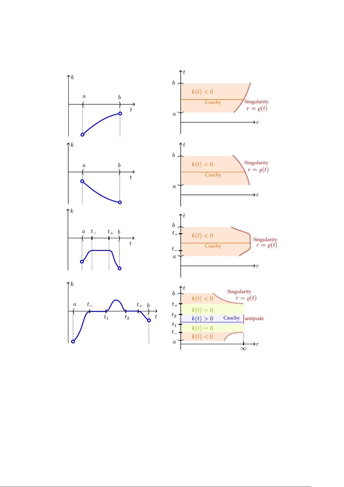
Cosmological Spacetimes with Sign-Changing Spatial Curvature and T op ological T ransitions Gera rdo Ga rc ´ ıa-Mo reno, 1 , 2 Bert Janssen, 3 Alejandro Jim´ enez Cano, 4 Ma rc Ma rs, 5 Miguel S´ anchez, 6 Ra¨ ul V era 7 1 Dip artimento di Fisic a, Sapienza Universit` a di R oma, Piazzale Aldo Mor o 5, 00185, R oma, Italy 2 INFN, Sezione di R oma, Piazzale A ldo Mor o 2, 00185, R oma, Italy 3 Dep artamento de F ´ ısic a T e´ oric a y del Cosmos and CAFPE, F acultad de Ciencias, Universidad de Gr anada, 18071 Gr anada, Sp ain 4 Escuela T´ ecnic a Sup erior de Ingenier ´ ıa de Montes, F or estal y del Me dio Natur al, Universidad Polit ´ ecnic a de Madrid, 28040 Madrid, Sp ain 5 Instituto de F ´ ısic a F undamental y Matem´ atic as, Universidad de Salamanc a Plaza de la Mer c e d s/n 37008, Salamanc a, Sp ain 6 Dep artamento de Ge ometr ´ ıa y T op olo g ´ ıa & IMAG, Universidad de Gr anada, 18071 Gr anada, Sp ain 7 Dep artment of Physics and EHU Quantum Center, Euskal Herriko Unib ertsitate a UPV/EHU, 48080 Bilb ao, Basque Country, Sp ain E-mail: gerardo.garciamoreno@uniroma1.it , bjanssen@ugr.es , alejandro.jimenez.cano@upm.es , marc@usal.es , sanchezm@ugr.es , raul.vera@ehu.eus Abstract: Observ ational evidence, together with practical computations and mo deling, supp orts a Euclidean spatial sector in the current cosmological mo del based on the FLR W metric. This, how ever, would imply that the total amoun t of matter and energy immediately after the Big Bang must hav e b een inﬁnite, an implication that could only b e a voided through a transition from a closed to an op en univ erse, a process forbidden in standard FLR W mo dels. In this article, we inv estigate the spacetimes resulting from promoting the spatial curv ature k in FLR W spacetimes to a time-dep enden t function, k → k ( t ), allo wing it to c hange sign and thereby allowing changes in the top ology of the constant- t slices. Although previously dismissed due to a classical theorem b y Gero c h, such transitions are shown to be consistent with global h yp erbolicity when the comoving time is distinct from a Cau ch y time, as recen t w ork by one of the authors demonstrates. W e construct three distinct geometries exhibiting this behavior using diﬀeren t represen tations of constant-curv ature spaces. W e analyze their global prop erties and iden tify mild conditions under which they remain globally hyperb olic. F urthermore, we c haracterize their Killing v ectors, pro ving a general result for spherically symmetric spacetimes and compare them with known geometries in the literature. Con tents 1 In tro duction 1 2 Global and lo cal roles of time in cosmological spacetimes 3 2.1 Deﬁning a cosmological spacetime 3 2.2 Global and lo cal time functions are indep enden t 6 2.3 Curren t Physics might require the disasso ciation of roles 7 3 Construction of the k ( t ) metrics and lo cal curv ature prop erties 8 3.1 FLR W metrics in sev eral coordinate systems 8 3.2 In tro ducing the k ( t ) metrics 9 3.3 Curv ature decomp osition for the k ( t ) metrics 10 3.4 Congruences 11 3.5 Singularities 12 3.5.1 The k ( t )-w arp ed case 12 3.5.2 The k ( t )-conformal case 13 3.5.3 The k ( t )-radial case 15 4 Smo oth extensions of the k ( t ) metrics 17 4.1 The k ( t )-w arp ed metric 17 4.2 The k ( t )-conformal metric 18 4.3 The k ( t )-radial metric 19 5 Global causal prop erties of the k ( t ) spacetimes 21 5.1 The k ( t )-w arp ed cosmological metric 23 5.2 The k ( t )-conformal cosmological spacetime 26 5.3 The k ( t )-radial cosmological spacetime 30 6 Killing vector ﬁelds 32 6.1 Necessary and suﬃcient conditions for FLR W metric 32 6.2 Killing v ector ﬁelds in spherically symmetric spaces (arbitrary dimension) 34 6.3 Killing v ector ﬁelds of the k ( t ) geometries 38 6.3.1 Pro of for the k ( t )-warped metric 40 6.3.2 Pro of for the k ( t )-conformal metric 41 6.3.3 Pro of for the k ( t )-radial metric 42 7 Comparing with other geometries 43 7.1 Inequiv alence among the three k ( t ) metrics 43 7.2 Comparison of the k ( t ) metrics with the Stephani universe 45 7.3 Comparison of the k ( t ) metrics with the Lema ˆ ıtre-T olman-Bondi metric 46 8 Summary of results 47 – i – 9 Discussion and conclusions 48 A Prop erties of the function S k ( t ) ( r ) 50 B Curv ature tensors for the k ( t ) metrics 51 B.1 Curv ature tensors for the k ( t )-w arp ed metric 51 B.2 Curv ature tensors for the k ( t )-conformal metric 52 B.3 Curv ature tensors for the k ( t )-radial metric 52 C Expansion, shear and vorticit y 53 C.1 k ( t )-warped metric 53 C.2 k ( t )-conformal metric 53 C.3 k ( t )-radial metric 53 1 In tro duction F riedman-Lema ˆ ıtre-Rob ertson-W alk er (FLR W) spacetimes oﬀer three fundamen tal bac k- ground geometries, spherical, ﬂat, and h yp erbolic, arising from general symmetry con- siderations prior to specifying the energy-momentum tensor. These assumptions can b e form ulated with mathematical precision leading to a rigidit y theorem c haracterizing these geometries (see, for instance, [ 1 , Ch. 12, Prop. 6]). How ever, many commonly cited ph ys- ical notions of homogeneit y and isotropy do not necessarily imply one of these standard cases. In fact, a recent example constructed b y one of the authors [ 2 ] and further examined b y ´ Av alos [ 3 ], demonstrates the p ossibilit y of foliating those spacetimes with spatial hy- p ersurfaces of constan t curv ature k ( t ) (and hence, maximally symmetric), where the sign of k ( t ) c hanges o ver time. The goal of this article is to show that such a scenario is not merely a mathemat- ical curiosity , but a p oten tially v aluable framew ork for mo dern cosmology . T o supp ort this, w e construct t wo additional classes of examples, derived from conv entional mo dels of spacetimes with constan t spatial curv ature, and study their prop erties, highligh ting cer- tain features that ma y pro v e adv antageous. W e analyze b oth global, namely , under whic h conditions they are globally h yp erbolic and nonsingular, as well as local prop erties, namely their isometries and curv ature prop erties. F urthermore, we show that the three of them are not isometric among them, nor to some geometries previously introduced in the literature, sp eciﬁcally the Stephani and the Lema ˆ ıtre-T olman-Bondi (L TB) geometries, since their energy-momen tum tensor is that of a p erfect ﬂuid and in the k ( t ) this implies FLR W, see Prop. 6.2 . The ﬁrst of the geometries, the k ( t ) -warp e d metric, is suc h that the point r = 0 is extrinsic al ly privileged (indeed, its expansion is v anishing in the simplest case, as the second fundamen tal form v anishes therein) and, when k ( t ) > 0, the an tip odal p oin t r = π / p k ( t ) is also privileged (the expansion div erges to wards this p oin t). The metric is automatically – 1 – smo oth at r = 0 but not at the t -antipo dal p oin ts. In [ 2 ], the metric w as deformed along a small region ar ound t -antipo dal p oin ts (maintaining the constant curv ature of the t - slices) so that it becomes smooth ev erywhere. Here, w e ha ve not used the smo othening and w e hav e analyzed the origin of non-smo othness: the scalar curv ature div erges and the metric cannot even be C 1 -extended to the t -antipo dal p oints (Prop. 4.1 , Rem. 4.2 ). The prop erties of this spacetime are in teresting because, on the one hand, they do not depend on smo othening and, on the other, the smo othed spacetimes coincide with the k ( t )-warped up to a region which can be c hosen arbitrarily small. Our second metric is called k ( t )- c onformal , b ecause its spatial metric is conformally isometric to the Euclidean one with conformal factor 4 / (1 + k ( t ) r 2 ) 2 . In addition, t -slices are totally umbilical. When k ( t ) > 0 the metric can b e smo othly extended to the p oin t at inﬁnit y (which corresp onds to stereographic compactiﬁcation). So, a completely classic smo oth cosmological spacetime is obtained (Prop. 4.3 ). F or our third metric, which we called the k ( t )- r adial , the spatial me tric is constructed b y changing the natural radial comp onent d r 2 of the Euclidean metric by d r 2 / (1 − k ( t )) r 2 . When k ( t ) > 0, the constan t t -slices are not a whole round sphere, but an op en subset of it, indeed, a half sphere (Prop. 4.4 , Rem. 4.5 ). So, they admit a c hange in the sign of the spatial curv ature, even if no topological change o ccurs. Our results rev eal that these geometries can b e considered as viable geometrical basis for cosmological mo dels. T o the b est of our knowledge, they hav e not b een previously rep orted in the literature, nor an y that exhibits similar properties. In particular, w e iden- tify the conditions under which they are globally hyperb olic, a fundamental requisite for describing a cosmological mo del. Additionally , for certain choices of the deﬁning functions, w e ﬁnd an explicit example that admits an extra Killing v ector. Structure of the article. The paper is structured as follows. In Sec. 2 we in tro duce the notion of cosmological model and discuss its prop erties, making a sp ecial emphasis on the necessary distinction betw een the global and lo cal ingredients. In Sec. 3 we in tro duce the spacetimes that we study in the article and present some of their local geometrical prop er- ties. In Sec. 4 we discuss the p ossibility to extend the geometries to p oints not co v ered b y the original co ordinates. In Sec. 5 we analyze the global prop erties of these geometries with a sp ecial emphasis on characterizing under which conditions global h yp erb olicit y holds. In Sec. 6 we c haracterize the isometries of the geometries, exhaustiv ely studying how many Killing v ectors exhibit dep ending on the functions en tering the metrics. In Sec. 7 w e com- pare these geometries with some previously studied mo dels, the L TB and the Stephani metrics, and sho w that they are not isometric. Finally w e summarize the main results of the article in Sec. 8 , and w e conclude in Sec. 9 b y explaining the opp ortunities that these metrics presen t for current Cosmology and discussing follo w-ups to this work. Notation and con v en tions. In this article, w e use the signature ( − , + , ..., +) for the spacetime metric and units in which c = G N = 1. F or the curv ature tensors we use the con v en tions in [ 4 ], i.e., [ ∇ a , ∇ b ] V d =: −R abc d V c , R ab := R acb c . W e call R the Ricci scalar, G ab := R ab − g ab R / 2 the Einstein tensor and C abcd the W eyl tensor. – 2 – Dots represent partial deriv ativ es with respect to the time co ordinate (or total deriv a- tiv e in case the function only dep ends on time) and primes corresp ond to the partial deriv ativ es with resp ect to the radial coordinates: ˙ X := ∂ t X , X ′ := ∂ r X . In the tensor expressions of the diﬀeren t metrics, w e abbreviate d X 2 := d X ⊗ d X and d X d Y := 1 2 (d X ⊗ d Y + d Y ⊗ d X ). Boldface sym b ols corresp ond to tensors, vector ﬁelds and diﬀeren tial forms in index- free notation. W e w ork in n + 1 spacetime dimensions. W e use h for the metric of the 2-dimensional base manifold of a warped product and γ for the standard S m metric, where m := n − 1 is the dimension of the ﬁb er S m . The symbol L n +1 will represent the Minko wski space time ( R 1 ,n equipp ed with the ﬂat metric). Finally w e summarize our index notation: • a, b, c, . . . are abstr act indic es in n + 1 dimensions (used essen tially to write an y tensor iden tit y without inv olving partial deriv atives, connections, etc.). These do not refer to an y sp eciﬁc basis and can apply to co ordinate bases, tetrads, etc. • µ, ν, ρ, . . . are indic es in a sp e ciﬁc c o or dinate b asis in n + 1 dimensions. In our case, w e use them to refer to comp onents in the c hart { x µ } = { t, r , θ A } (see b elow for the deﬁnition of θ A ). • i, j, k , . . . are indic es in a sp e ciﬁc c o or dinate b asis { y i } = { t, r } on the 2-dimensional b ase sp ac e . • A, B , C, . . . are indic es on the spher e S m , and corresp ond to the hyperspherical coor- dinates (denoted as θ A ). • I , J , K are indic es in the Euclide an ( m + 1) -dimensional sp ac e where S m is canonically em b edded. • a , b are indic es in the Kil ling algebr a of the base space and run from 1 to n . 2 Global and lo cal roles of time in cosmological spacetimes 2.1 Deﬁning a cosmological spacetime T o start with, it is con venien t to recall that a cosmological mo del should not simply b e though t as a spacetime, i.e., a manifold with a Lorentzian metric, but it also needs tw o additional k ey ingredients: a description of matter and radiation, and a uniquely deﬁned set of fundamental (also called comoving) observ ers u that are to describ e the av erage motion of matter in the universe, in terms of which observ ational relations are set b etw een the geometry and the matter con tent [ 5 ]. Keeping only the geometrical ingredients, and in a slightly simpliﬁed fashion enough for the purp oses of this work, following [ 6 ] (see also [ 3 ]) w e say a Lorentzian manifold ( V n +1 , g ), n ≥ 3, is a c osmolo gic al sp ac etime if – 3 – • V n +1 = I × Σ n , where I is a connected op en interv al of R , whic h we parametrize by some co ordinate t , • u = ∂ t is orthogonal to the leav es { t } × Σ n and g ( u , u ) = − 1. The vector ﬁeld u represen ts the comoving observers, which usually are assumed to b e freely-falling (this will hold in our mo dels too). In fact, this means that a single Lorentzian manifold can p oten tially giv e rise to diﬀerent cosmological spacetimes, eac h one asso ciated with diﬀeren t c hoices of comoving observers. de Sitter spacetime as a pla yground for diﬀerent cosmological spacetimes. W e can illustrate this with a simple example. W e deﬁne the ( n + 1)-dimensional de Sitter spacetime as the submanifold embedded in L n +2 describ ed by −  X 0  2 + n +1 X i =1  X i  2 = ℓ 2 , (2.1) with the induced metric inherited from the ﬂat metric g L n +2 = − (d X 0 ) 2 + n +1 X i =1 (d X i ) 2 . (2.2) The de Sitter spacetime is a solution of the Einstein equations in v acuum with p ositive cosmological constan t, where Λ = n ( n − 1) / (2 ℓ 2 ). There are diﬀeren t coordinate systems that bring de Sitter to an FLR W form. In par- ticular, w e can tak e the closed slicing, whic h foliates de Sitter with n -dimensional spheres, b y setting X 0 = ℓ sinh  T ℓ  , (2.3) X 1 = ℓ cosh  T ℓ  cos( ϑ ) , (2.4) X i = ℓ cosh  T ℓ  sin( ϑ ) ˆ n i ( θ A ) , i = 2 , ..., n + 1 , (2.5) where ˆ n i represen ts the outw ard unit vector orthogonal to S n − 1 ⊂ R n in terms of the co ordinates { θ A } of the sphere. The range of the time co ordinate is T ∈ R , ϑ ∈ (0 , π ) is a colatitude angle on the n -sphere and, as already men tioned, { θ A } are standard co ordinates in the ( n − 1)-spheres. The metric in these co ordinates reads g dS = − d T 2 + ℓ 2 cosh 2  T ℓ   d ϑ 2 + sin 2 ( ϑ ) γ  , (2.6) where w e notice that the part in square brack ets is the standard metric on the n -dimensional sphere S n . This co ordinate representation of the de Sitter spacetime exhibits a foliation in whic h the area of the ( n − 1)-dimensional spheres tends to inﬁnity for T → −∞ , monoton- ically decreases to a minimum at T = 0, and then monotonically increases all the wa y to inﬁnit y as T → + ∞ . – 4 – N o r t h P o l e S o u t h P o l e N o r t h P o l e S o u t h P o l e Figure 1 . F oliations of the de Sitter spacetime ( n ≥ 2) represen ted in a P enrose diagram: the spherical foliation b y constant- T slices (left), whic h co vers the en tire spacetime, and the foliation by ﬂat constant- t slices (right), which co v ers only half of it. Note that, in the latter case, there exists an analogous foliation of the other half of the spacetime, but the t w o cannot b e smo othly joined to form a global one, since the surface X 0 + X 1 = 0 is n ull (solid blac k line in the right panel). The arro ws represen t the corresp onding comoving observ ers. Dashed lines represent constant- ϑ ( r ) in the left (right) panel. On the other hand, w e can tak e the ﬂat slicing in terms of a set of coordinates ( t, x I ) ≡ ( t, r, θ A ), where { x I } represent the Cartesian co ordinates in Euclidean space and ( r, θ A ) are the corresp onding radial and hyperspherical coordinates, by ﬁxing X 0 = ℓ sinh  t ℓ  + r 2 2 ℓ e t/ℓ , (2.7) X 1 = ℓ cosh  t ℓ  − r 2 2 ℓ e t/ℓ , (2.8) X i = e t/ℓ r ˆ n i ( θ A ) , i = 2 , ..., n + 1 . (2.9) The metric in these co ordinates is giv en by g dS = − d t 2 + e 2 t/ℓ (d r 2 + r 2 γ ) . (2.10) This cov ers the region X 0 + X 1 > 0 of the hyperb oloid with planes t = constant intersecting it at 45 ◦ (see [ 7 , Sec. 5.2]). T o cov er the remaining part, we can choose another similar patc h of coordinates, resulting simply in an exc hange of the time co ordinate t → − t in the metric. F rom these tw o foliations, we see that within the same manifold we can tak e t w o (actually more) vector ﬁelds u that represen t the comoving time, namely ∂ T and ∂ t . Clearly , b oth vectors are diﬀerent, as the t wo sets of coordinates are related through e t/ℓ = sinh  T ℓ  + cos( ϑ ) cosh  T ℓ  , (2.11) e t/ℓ r = ℓ cosh  T ℓ  sin( ϑ ) , (2.12) – 5 – while θ A remain unchanged. In other words, diﬀerent sets of observ ers can b e taken as the fundamen tal, or comoving, ones. Even though this can b e done in de Sitter spacetime due to its high level of symmetry , it highligh ts the crucial role that the choice of comoving time pla ys in deﬁning a cosmology . Another in teresting example is the Milne spacetime which also stresses the importance of the comoving observers. In fact, it sho ws that even an op en subset of Mink o wski space- time (the c hronological future of a point) can b e regarded as a non-trivial cosmological mo del. Predictabilit y . In addition to this, a cosmological spacetime should also fulﬁll a global fundamen tal property: pr e dictability . This feature is adequately captured b y the notion of glob al hyp erb olicity , which can b e deﬁned in diﬀeren t w ays such as unique evolution from initial data p osed on a Cauch y hypersurface, absence of naked singularities and others (see [ 8 , 9 ]) 1 . A celebrated theorem by Gero ch [ 12 ] reﬁned b y Bernal and S´ anc hez [ 13 , 14 ], pro v es that a globally hyperb olic spacetime admits a smo oth Cauch y temp oral function τ , so that the spacetime manifold splits globally as an orthogonal pro duct ( I × S , g ). Here, I ⊂ R is an in terv al and the metric takes the form g = − λ ( τ , x )d τ 2 + g τ [ x ] , (2.13) where eac h slice { τ 0 } × S , τ 0 ∈ I , inherits a p ositiv e-deﬁnite metric g τ 0 and turns out to b e a smo oth spacelike Cauc hy h yp ersurface. F rom a purely mathematical viewp oint, there is a h uge freedom to choose such a τ . 2 Notice that the splitting in Eq. ( 2.13 ) and the one app earing in the deﬁnition of cosmological spacetime do not necessarily need to agree. They do agree in the standard FLR W models, since the como ving time pla ys not only a global role (constant t -slices are Cauc h y and pro vide a global splitting), but also a lo cal role as the slices are maximally symmetric and hence hav e constant curv ature. As men tioned ab ov e, the freedom to choose a Cauch y temp oral function is huge and, th us, this lo cal symmetry condition which is sometimes link ed to physical magnitudes (as it happ ens in the FLR W case, see for example [ 17 ]) selects a sp ecially appropriate time, t ypically unique. 2.2 Global and lo cal time functions are indep enden t Coming to our example in de Sitter spacetime, the closed slicing gives rise to a globally deﬁned foliation in which the constant como ving time surfaces are Cauc h y hypersurfaces (they are compact). The ﬂat slicing though, is suc h that the comoving time gives rise to noncompact hypersurfaces which clearly cannot b e Cauch y surfaces of the de Sitter spacetime as deﬁned ab ov e (since all Cauch y surfaces are homeomorphic). In that sense, 1 When global hyperb olicity fails, one should add “information at conformal inﬁnit y”, as o ccurs in the case of anti-de Sitter spacetime. This situation can b e handled with the notion of globally hyperb olic spacetime-with-timelik e-b oundary developed in [ 10 , 11 ]. Here w e will focus in the case without b oundary for simplicity (but see fo otnote 12 in Rem. 5.13 regarding the k ( t )-radial case). 2 This w as stressed in [ 15 ] where, for example, an y compact acausal spacelik e submanifold with boundary is shown to lie in a τ -slice for some Cauc hy temp oral τ . The freedom in τ had already led Andersson et al. to prop ose a wa y to construct a “standard cosmological time” [ 16 ] for quite general spacetimes. – 6 – the example shows that b oth times do not necessarily need to agree. Ho w ever, this is actually pathological from the global p oin t of view, as the ∂ t v ector ﬁeld cannot be extended con tin uously at t → −∞ and hence it is not p ossible to smo othly connect it with another v ector ﬁeld deﬁned in the other half-part of de Sitter. In fact, time functions that attempt to smoothly in terp olate from the closed to the op en slicing in de Sitter spacetime hav e b een previously rep orted by Krasi ´ nski taking co ordinates in which the metric b elongs to the Stephani family [ 18 , 19 ], see also [ 20 , 21 ]. F urthermore, other solutions describing less symmetric spacetimes that in principle allow for this disso ciation of roles hav e been rep orted [ 22 , 23 ]. This already suggests that the t wofold role pla yed b y time in FLR W spacetimes should not b e tak en as mandatory , as it is actually not needed. In fact, w e w an t to highligh t the inheren t indep endence b et w een tw o diﬀerent prop erties implicitly assumed for the “spatial part” of cosmological spacetimes so far: (a) Existence of a temp oral function with a constant curv ature slicing (motiv ated by considerations on intrinsic isotropy and homogeneit y). (b) Existence of a Cauch y temp oral function t (motiv ated by considerations on pre- dictabilit y), that is, inextensible causal curves, whic h represen t particles, must cross eac h spatial t -slice exactly once. In fact, whereas the top ology of Cauch y slices (b) is ﬁxed, there is no requirement that the top ology of the constant curv ature slices (a) needs to b e ﬁxed. This means that mo dels in whic h the topology of the constan t curv ature slices c hanges (our k ( t ) metrics allow this p ossibilit y) will admit some temporal functions fulﬁlling (a) and others fulﬁlling (b) but none fulﬁlling b oth. 2.3 Curren t Physics migh t require the disasso ciation of roles The diﬀeren t roles for the spatial slicing p ointed out in (a) and (b) ab ov e are clearly distinguished from a purely physical viewpoint. The property (a) is a strong assumption with local nature. In principle, the time whic h pro duces suc h a constan t curv ature slicing should b e then tied to some locally measurable ph ysical pro cess or magnitude. Ho w ev er, the property (b) is a mathematical consequence of predictability , which has a philosophical rather than ph ysical nature: we ma y b eliev e that the present determines the future (in a mathematically precise wa y), but only omniscent observers could c heck it. Indeed, very general acausal subsets b ecome a part of a slice for some Cauc hy temp oral function τ (recall fo otnote 2 ) but no lo cal measuremen t could determine the whole slice. More down-to-earth, the disso ciation of b oth roles in some of our cosmological space- times with c hanging k ( t ) p ermits to mo del app ealing cosmological possibilities, such as a Big-Bang in a closed mo del which ma y seem an op en mo del for como ving observers later. – 7 – 3 Construction of the k ( t ) metrics and lo cal curv ature prop erties W e b egin this section by reviewing the FLR W metric, as the v arious p ossible co ordinate c hoices on the spatial slices serv e as the starting p oint for constructing the metrics analyzed in this article. 3.1 FLR W metrics in sev eral co ordinate systems The metric of FLR W spacetimes in como ving coordinates takes the form g FLR W = − d t 2 + a ( t ) 2 ˜ g t , (3.1) where t is the comoving time, a ( t ) the scale factor, and ˜ g t the metric of constant (time indep enden t) curv ature spatial sections. It is w ell kno wn that there are only three pos- sibilities, 3 dep ending on the sign of the curv ature: in three dimensions p ositive constant curv ature spaces are 3-spheres S 3 , negativ e constant curv ature spaces are hyperb oloids H 3 and the zero curv ature space is ﬂat Euclidean space R 3 . Concretely , for k > 0 the metric ˜ g t describ es a 3-sphere with curv ature radius 1 / √ k , for k < 0 a hyperb olic space with curv ature radius 1 / √ − k and k = 0 is Euclidean space. Diﬀeren t co ordinate systems can b e used to describ e the spatial hypersurfaces, for instance w e hav e the three following p ossibilities: g FLR W = − d t 2 + a ( t ) 2  1 1 − k r 2 d r 2 + r 2 γ  (3.2) = − d t 2 + a ( t ) 2  d χ 2 + F ( χ ) 2 γ  (3.3) = − d t 2 + 4 a ( t ) 2 (1 + k R 2 ) 2  d R 2 + R 2 γ  , (3.4) where the diﬀerent radial co ordinates are related by: r = S k ( χ ) = 2 R 1 + k R 2 , (3.5) and with the function S k ( χ ) deﬁned as S k ( χ ) :=                sin  √ k χ  √ k if k > 0 χ if k = 0 sinh  √ − k χ  √ − k if k < 0 . (3.6) A rigidit y theorem for FLR W is presen ted in [ 1 ], where it is shown that FLR W can be c haracterized as the set of cosmological spacetimes that are isotropic, where isotrop y should b e understo o d in the sense of spacetime isotrop y as deﬁned in [ 3 ]. 3 Up to taking the quotient by a discrete subgroup of the symmetry group, eﬀectiv ely changing the top ology of the spatial slices [ 24 ]. – 8 – As carefully analyzed in [ 3 ], it has sometimes been incorrectly stated in the literature that FLR W spacetimes are simply those that are spatially homogeneous and isotropic (observ e that no w “isotropy” is understo o d in the sense of spatial isotropy), that is, that eac h constant-time slice inherits an induced metric that is maximally symmetric. In fact, w e can see that the existence of a foliation with maximally symmetric slices do es not lead to the rigidit y of FLR W spacetimes b y pro viding three straightforw ard counterexamples. Any promotion of the in trinsic curv ature of the spatial slices in Eqs. ( 3.2 )-( 3.4 ) to a time function k → k ( t ) leads to a counterexample. Indeed, among other local and global prop erties, w e will see that none of the three resulting spacetimes is isometric to a patc h of FLR W or eac h other (previous examples app ear in [ 2 ], see also [ 25 ]). 3.2 In tro ducing the k ( t ) metrics Let I ⊂ R b e an op en interv al and a, k : I → R any smo oth functions with a > 0. Consider the following metrics on some op en subsets U of I × R n , whic h are deﬁned by taking spherical co ordinates ( r, θ A ) in R n (the con ven tion 1 / √ C = ∞ if C ≤ 0 is used): 1. The k ( t )-warped metric g war = − d t 2 + a ( t ) 2  d r 2 + S 2 k ( t ) ( r ) γ  , (3.7) where γ is the standard metric on S n − 1 , the domain of the co ordinates is U war = ( ( t, r, θ A ) : t ∈ I , 0 < r < π p k ( t ) ) (3.8) and the function S k ( r ) has b een introduced in Eq. ( 3.6 ). 2. The k ( t )-conformal metric: g con = − d t 2 + 4 a ( t ) 2 (1 + k ( t ) r 2 ) 2  d r 2 + r 2 γ  , (3.9) where the { t, r } take v alues in U con = ( ( t, r, θ A ) : t ∈ I , 0 < r < 1 p − k ( t ) ) . (3.10) 3. The k ( t )-radial metric: g rad = − d t 2 + a ( t ) 2  1 1 − k ( t ) r 2 d r 2 + r 2 γ  , (3.11) where the { t, r } take v alues in U rad = ( ( t, r, θ A ) : t ∈ I , 0 < r < 1 p k ( t ) ) . (3.12) – 9 – In the three cases we will collectiv ely denote b y x = ( r , θ A ) the spacelike co ordinates. W e no w turn our attention to their local geometric prop erties, focusing on the curv ature tensors and the b ehavior of the congruence of integral curv es of the geo desic vector ﬁeld ∂ t . The discussion of whether these geometries can b e extended to the boundary of the in terv al ov er which r is deﬁned on eac h case will be postp oned un til Sec. 4 . 3.3 Curv ature decomp ositi on for the k ( t ) metrics The geometries given b y the k ( t ) metrics hav e the structure of a warped pro duct with ﬁb er S n − 1 and base manifold N an op en neigh b orho o d of R 2 . T o b e precise, the total manifold admits a lo cal pro duct decomp osition N × S n − 1 , and the metric tensor has the form g = h + f 2 γ , (3.13) with h = h ij ( y )d y i d y j = − d t 2 + W 2 d r 2 , (3.14) γ = γ AB ( θ )d θ A d θ B . (3.15) The w arping functions f are giv en by f ( t, r ) =          a ( t ) S k ( t ) ( r ) k ( t )-warped metric a ( t ) 2 r 1 + k ( t ) r 2 k ( t )-conformal metric a ( t ) r k ( t )-radial metric (3.16) and the functions W are W ( t, r ) =                a ( t ) k ( t )-warped metric a ( t ) 2 1 + k ( t ) r 2 k ( t )-conformal metric a ( t ) 1 p 1 − k ( t ) r 2 k ( t )-radial metric . (3.17) Giv en that the ﬁb er is an ( n − 1)-sphere of unit radius (hence maximally symmetric with constan t curv ature equal to one), the Ricci tensor of the ﬁb er is R ( γ ) AB = ( n − 2) γ AB . (3.18) On the other hand, the comp onen ts of the Ricci tensor and the Ricci scalar of the base space can b e easily computed: R ( h ) tt = − ¨ W W , R ( h ) tr = 0 , R ( h ) rr = W ¨ W , (3.19) R ( h ) = 2 ¨ W W . (3.20) – 10 – No w w e can mak e use of w ell-kno wn expressions for the Ricci tensor of a warped pro duct (see e.g. [ 1 , Cor. 7.43]) to ﬁnd the comp onen ts of the Ricci tensor of the total space: R tt = − ¨ W W − ( n − 1) ¨ f f , (3.21) R tr = ( n − 1) " ˙ W f ′ W f − ˙ f ′ f # , (3.22) R rr = W ¨ W + ( n − 1) " W ˙ W ˙ f f + W ′ f ′ W f − f ′′ f # , (3.23) R tA = R rA = 0 , (3.24) R AB = " f ¨ f + ˙ W W f ˙ f − f f ′′ W 2 + W ′ f f ′ W 3 + ( n − 2)  1 + ˙ f 2 − f ′ 2 W 2  # γ AB . (3.25) The Ricci scalar is then given b y R = 2 ¨ W W + 2( n − 1) ¨ f f − f ′′ W 2 f + ˙ W ˙ f W f + W ′ f ′ W 3 f ! + ( n − 1)( n − 2) f 2  1 + ˙ f 2 − f ′ 2 W 2  . (3.26) The explicit expressions for the sp eciﬁc metrics g con , g war and g rad can be found in App. B . 3.4 Congruences W e can take the v ector u a = ( ∂ t ) a and analyze the b ehavior of the congruence of its in tegral curv es. W e start b y constructing the tensor: B ab := ∇ b u a , (3.27) Since the one form u a is closed (d u = 0) it follo ws that B ab is symmetric. F rom u b eing unit w e get B ab u a = 0, so B ab is purely spatial, i.e., u a B ab = u a B ba = 0, and u a is geo desic. The information about the inﬁnitesimal b eha vior of the congruence is enco ded in the irreducible parts of B ab whic h are called vorticit y , shear and expansion and are resp ectively given b y ω ab := 1 2 ( B ab − B ba ) , (3.28) σ ab := 1 2 ( B ab + B ba ) − 1 n Θ s ab , (3.29) Θ := g ab B ab , (3.30) where s ab := g ab + (d t ) a (d t ) b is the spatial part of the metric. In our case, the vorticit y v anishes identically and the comp onents B µν in the chart { x µ } = { t, r , θ A } are purely spatial and read: B µν = ∂ ν u µ − Γ ρ ν µ u ρ = Γ t ν µ = 1 2 ∂ t s µν . (3.31) – 11 – Using s µν d x µ d x ν = W 2 ( t, r )d r 2 + f 2 γ AB d θ A d θ B , the only non trivial comp onents B µν are B rr = W ˙ W , B AB = f ˙ f γ AB . (3.32) Th us, the expansion, the non-v anishing components of the shear tensor and the shear scalar σ 2 := σ µν σ µν read Θ = ˙ W W + ( n − 1) ˙ f f , (3.33) σ rr = n − 1 n W 2 ˙ W W − ˙ f f ! , σ AB = − 1 n f 2 ˙ W W − ˙ f f ! γ AB , (3.34) σ 2 = n − 1 n ˙ W W − ˙ f f ! 2 . (3.35) Notice that the shear v anishes in the FLR W case, as it should. Inserting the sp eciﬁc form of f , W one ﬁnds the expansion and shear for eac h of the metrics. W e collect the results in App. C . Finally , w e present another relev an t quantit y that will b e used in the following to analyze the spacetime close to singular regions. As a measure of the tidal forces, we consider the relativ e acceleration of tw o nearby test particles that follo w geo desics of the como ving observers ∂ t . This can b e computed via the geo desic deviation equation given b y ∇ 2 V a d t 2 = R bcd a V b ( ∂ t ) c ( ∂ t ) d , (3.36) where V a is a deviation v ector, satisfying [ V , ∂ t ] = 0. If we fo cus on particles separated along the r direction, at the initial time of deviation t 0 w e ﬁnd ∇ 2 V µ d t 2     t = t 0 = R rtt µ | t = t 0 , (3.37) since V µ | t 0 = ( ∂ r ) µ = δ µ r in the co ordinates { t, r , θ A } . All these expressions are v alid for the three k ( t ) metrics. 3.5 Singularities In the three cases, the metrics w ere deﬁned on an op en subset of I × R n in Sec. 3.2 , and they are smo othly extensible to r = 0. How ever curv ature singularities may appear at the maxim um v alue of r making the metric inextensible therein (at leas t as a C 2 metric). In the follo wing we analyze case b y case and study in detail the diﬀerences b etw een them. 3.5.1 The k ( t ) -w arp ed case Prop osition 3.1. The k ( t ) -warp e d metric with k ( t ) > 0 and ˙ k ( t )  = 0 exhibits a curvatur e singularity at the antip o dal p oint r → π / p k ( t ) . – 12 – Pr o of. Consider a time in terv al in which k ( t ) > 0 and ˙ k ( t )  = 0. Using ( B.5 ), w e ﬁnd the follo wing expression: R = α 0 ( t ) + α 1 ( t ) ˆ r 2 + α 2 ( t ) ˆ r cot( ˆ r ) + α 3 ( t ) ˆ r 2 cot 2 ( ˆ r ) , ˆ r := p k ( t ) r , (3.38) for certain functions α 0 , α 1 , α 2 and α 3 . The antipo dal p oint corresp onds to the limit ˆ r ↗ π (at a ﬁxed time). As we approac h suc h a limit for a ﬁxed time, we ﬁnd the leading asymptotic b ehavior is R ∼ α 3 ˆ r 2 cot 2 ( ˆ r ) ( ˆ r ↗ π ) , (3.39) where α 3 = ( n − 1)( n − 2) 4 ˙ k 2 k 2  = 0 (3.40) due to the hypothesis ˙ k  = 0. Consequen tly , the Ricci scalar diverges as w e approach the an tip o dal p oint. ■ Ho w ev er, following the approac h in [ 2 , Sec. 4], it is p ossible to introduce a nonsingular geometry (a smo othening ) that agrees with the k ( t )-warped line-element everywhere but at a small open neigh b orho o d near the antipo dal point and preserv es the global properties of the spacetime (more on this in Prop. 4.1 b elo w). The geo desic deviation equation ( 3.37 ) for the k ( t )-w arp ed metric reads, at an y initial time t 0 , ∇ 2 V µ d t 2     t = t 0 = ¨ a a     t = t 0 δ µ r . ( 3.41) This tidal acceleration is ﬁnite ev erywhere. This sho ws the mildness of this singularit y and the p ossibilit y to smo othen it as in [ 2 ] in a simple wa y (in that reference a ( t ) was constan t so that the geo desic deviation identically v anished). After the smoothening, there still remains an unremov able singularity that app ears along a como ving observer lying at the antipo dal point as k ( t ) ↘ 0. Indeed, even when, say , k ( t 0 ) = 0 and ˙ k ( t 0 ) < 0, the an tip o dal point must b e remo v ed at t = t 0 , whic h underlies the top ological c hange in the spatial part. The singularity is similar to the one that app ears in the k ( t )-conformal case, but in a someho w more symmetric w ay: the space around the comoving observer would b e growing so fast that they would need to disapp ear in ﬁnite prop er time. 3.5.2 The k ( t ) -conformal case Prop osition 3.2. The k ( t ) -c onformal metric is lo c al ly c onformal ly ﬂat. Pr o of. This can be shown by directly computing the W eyl tensor which turns out to be iden tically v anishing (indep endently of the spatial dimension n ≥ 3). ■ As a consequence of the previous result, all the curv ature prop erties are hence enco ded in the Ricci tensor. Prop osition 3.3. Consider a k ( t ) -c onformal metric with k ( t ) < 0 and ˙ k ( t )  = 0 . – 13 – finite proper time infinite spatial distance S i n g u l a r i t y Figure 2 . Spacetime diagram that shows the situation of the cosmological como ving observ er of the k ( t )-conformal metric hitting the curv ature singularity at r → 1 / p − k ( t ) whenever | k ( t ) | increases in a certain interv al. As indicated in the picture, such a singularit y is alwa ys at an inﬁnite spatial distance (along the ∂ r direction) from any of these observ ers but is reached in a ﬁnite prop er time for any of them at suﬃcien tly large distance from the origin r = 0. (1) The sp ac etime exhibits a curvatur e singularity at the antip o dal p oint r → 1 / p − k ( t ) . (2) If ˙ k < 0 , the c omoving observers ∂ t at suﬃciently high r r e ach the singularity in ﬁnite pr op er time. (3) The sp atial distanc e along ∂ r curves b etwe en an event at t = t 0 and r = r 0 < 1 / p − k ( t 0 ) and the singularity is inﬁnite. Pr o of. (1) Immediate from the expression of the Ricci scalar ( B.16 ), whic h blo ws up at that p oin t as long as ˙ k  = 0 and k < 0. (2) Fix an y time t 1 . Since ˙ k < 0, the minim um of | k | in the domain t < t 1 is reached at t = t 1 . Let r 0 > 0 b e deﬁned by r 2 0 = − 1 /k ( t 1 ). The range of v alues of the coordinate r for which the metric is deﬁned shrinks as t increases. An observer along ∂ t at a v alue r > r 0 will reach the singularity at the an tip o dal p oin t b efore t = t 1 , hence in ﬁnite prop er time. (3) A direct computation leads to: Z 1 / √ − k ( t 0 ) r 0 √ g rr d r = 2 a ( t 0 ) Z 1 / √ − k ( t 0 ) r 0 d r 1 + k ( t 0 ) r 2 = ∞ . (3.42) ■ The singular b ehavior can also be seen from the follo wing fact: – 14 – finite proper time finite spatial distance S i n g u l a r i t y Figure 3 . Spacetime diagram that shows the situation of the cosmological como ving observer of the k ( t )-radial metric hitting the curv ature singularity at r → 1 / p k ( t ) whenev er k ( t ) increases in a certain in terv al. As indicated in the picture, the singularity is hit in a ﬁnite prop er time b y the observ ers ∂ t at suﬃciently large distance from the origin r = 0. Prop osition 3.4. The singularity of the k ( t ) -c onformal metric with k ( t ) < 0 and ˙ k ( t )  = 0 is such that the tidal for c es and the exp ansion of the c ongruenc e of c omoving observers deﬁne d by ∂ t diver ge as r → 1 / p − k ( t ) at c onstant t . Pr o of. The ﬁrst term in the expression of the expansion ( C.3 ) is ﬁnite as in FLR W, but the second term blows up as r → 1 / p − k ( t ). F or the k ( t )-conformal metric, the geo desic deviation ( 3.37 ) reads, at initial deviation, ∇ 2 V µ d t 2     t = t 0 = ¨ a a − r 2 (2 ˙ a ˙ k + a ¨ k ) a (1 + k r 2 ) + 2 r 4 ˙ k 2 (1 + k r 2 ) 2 !      t = t 0 δ µ r , (3.43) so the tidal forces are indeed divergen t as r → 1 / √ − k unless ˙ k = 0. ■ This singularity can b e interpreted in the follo wing w ay . If k is negative and decreas- ing, the spatial sections b ecome more and more hyperb olic, in the sense that the same displacemen t in the radial co ordinate corresp onds to an increasingly larger prop er dis- tance. This happens in such a w ay that the separation betw een tw o close freely-falling observ ers gro ws un til the one at bigger r disapp ears from the spacetime (it being pushed to inﬁnity), so the spacetime b ecomes timelik e geo desically incomplete. See Fig. 2 , for a pictorial represen tation of the singularity . 3.5.3 The k ( t ) -radial case Prop osition 3.5. Consider a k ( t ) -r adial metric with k ( t ) > 0 and ˙ k ( t )  = 0 . (1) The sp ac etime exhibits a curvatur e singularity at r → 1 / p k ( t ) , wher e b oth the Ric ci sc alar and the sc alar C abcd C abcd b e c ome inﬁnite. (2) If ˙ k ( t ) > 0 , the c omoving observers ∂ t at suﬃciently high r r e ach the singularity in ﬁnite pr op er time. – 15 – (3) The sp atial distanc e along ∂ r curves b etwe en the singularity at t = t 0 and an event at t = t 0 and r = r 0 < 1 / p k ( t 0 ) is ﬁnite. Pr o of. (1) Immediate from the expression of the Ricci scalar Eq. ( B.25 ), whic h blows up at that p oin t provided ˙ k  = 0 and k > 0. W e can compute the square of the W eyl tensor to obtain C abcd C abcd = n − 2 n  r 2 1 − k r 2  ˙ a a ˙ k + ¨ k  + 3 r 4 2(1 − k r 2 ) 2 ˙ k 2  2 , (3.44) whic h also b ecomes inﬁnite at the limit r → 1 / √ k . (2) The como ving time t measures prop er time for the geo desic obse rv ers deﬁned by ∂ t . Fix an y time t = t 1 . When ˙ k > 0, the v alue of k increases and the radius at which the singular b ehavior app ears decreases with time. An observer in an orbit r = r 0 with r 0 > 1 / p k ( t 1 ) will hit the singularity b efore t = t 1 and hence at ﬁnite prop er time. (3) In this case, w e ﬁnd: Z r max r 0 √ g rr d r = a ( t 0 ) r max  π 2 − arcsin  r 0 r max  (3.45) with r max := 1 / p k ( t 0 ). ■ Notice that the divergence of the square of the W eyl tensor at r = r max , whic h only encapsulates information of the conformal structure of the geometry , points to the fact that the ligh tcone structure itself is suﬀering a w eird phenomenon there. In fact, w e will later see that the lightcones degenerate at the singularit y . Prop osition 3.6. The singularity of the k ( t ) -r adial metric with k ( t ) > 0 and ˙ k ( t )  = 0 is such that the tidal for c es, the exp ansion and the she ar of the c ongruenc e of c omoving observers deﬁne d by ∂ t diver ge as r → 1 / p k ( t ) . Pr o of. The expansion and the shear scalar σ 2 of the congruence asso ciated to ∂ t b ecome inﬁnite as r → 1 / √ k , cf. Eqs. ( C.5 )-( C.6 ). In this case, the expression for the tidal forces ( 3.37 ) reads ∇ 2 V µ d t 2     t = t 0 = " ¨ a a + r 2 (2 ˙ a ˙ k + a ¨ k ) 2 a (1 − k r 2 ) + 3 r 4 ˙ k 2 4(1 − k r 2 ) 2 #      t = t 0 δ µ r , (3.46) whic h clearly diverges as r → 1 / √ k . ■ Notice that even though the expression ( 3.46 ) is qualitatively similar to the one ob- tained in the k ( t )-conformal case ( 3.43 ), in this case the situation is qualitatively diﬀerent from a causal p oint of view (see e.g. Lem. 4.7 ). – 16 – 4 Smo oth extensions of the k ( t ) metrics In this section we study the possibility of extending the metrics to r = 0 and to the upp er limit of r . F or the latter, w e fo cus on the case k ( t ) > 0 (including r = ∞ for g con ), since the constant- t slices correspond to a domain of a sphere that migh t a priori be extendible across its b oundary . On the other hand, for k ( t ) ≤ 0 the top ology of these spatial slices is R n and the upp er limit of r is already at inﬁnit y . Decomp ose I = I + ∪ I ≤ 0 , where I + := { t ∈ I : k ( t ) > 0 } , I ≤ 0 := { t ∈ I : k ( t ) ≤ 0 } (= I \ I + ) , (4.1) and let us consider separately the three cases. Notice that in the three cases w e hav e g = − d t 2 + a ( t ) 2 ˜ g t = a ( τ ) 2  − d τ 2 + ˜ g t ( τ )  , (4.2) where w e hav e introduced the co ordinate τ by d τ = d t a ( t ) . (4.3) In this section and the following one we study extendibilit y and global prop erties of the spacetimes. Those results that hold for the metric g will also hold for the metric − d τ 2 + ˜ g t ( τ ) as long as the function a ( t ) is non v anishing. In fact, for the rest of this section and the follo wing one w e set a ( t ) = 1. The only place where this may hav e a p otential eﬀect is regarding the prop erties of the conformal b oundary app earing in the k ( t )-radial spacetime, where it can change the causal character of the b oundary dep ending on whether the range of the co ordinate τ is b ounded (leading to a natural conformal b oundary that is spacelik e). See Rem. 4.9 b elow. 4.1 The k ( t ) -w arp ed metric Prop osition 4.1. The metric g war is smo oth on U war ∪ { r = 0 } , but it c annot b e smo othly extende d to r = π / p k ( t ) whenever k ( t ) > 0 , ˙ k ( t )  = 0 . However, g war c an b e deforme d in an arbitr arily smal l r e gion U π ar ound r = π / p k ( t ) , so that: (a) the deforme d metric b e c omes smo oth on I + × S n and, so, on the manifold obtaine d as the union ( I + × S n ) ∪ ( I ≤ 0 × R n ) , and (b) e ach spheric al slic e { t 0 } × S n , t 0 ∈ I + , is endowe d with a Riemannian metric of c onstant curvatur e k ( t 0 ) . This deformation wil l b e c al le d a smo othening of g war on U π . Pr o of. The required smo othness of g war at r = 0 w as prov en in [ 2 , Thm. 3.1]. The singu- larit y at r = π / p k ( t ) (see Prop. 3.1 ) makes g war C 2 -inextensible therein. When I + is an in terv al, the smo othenings with the stated prop erties (a) and (b) w ere carefully constructed in [ 2 , Sec. 4]. Otherwise, as I + is op en it can b e written as the union of op en disjoint interv als the pro cedure can b e applied to eac h of them. ■ – 17 – Notice that U π can b e regarded as “small” and irrelev an t for our purposes. 4 Remark 4.2. The previous pro of shows C 2 -inextendibilit y , but the follo wing computations deep en in the mo del by pro ving ev en C 1 -inextendibilit y . Replace r b y the co ordinate ˆ r = p k ( t ) r ( < π ) in U war ∩ ( I + × R n ), whic h was in tro duced in ( 3.38 ). Then d ˆ r =  ∂ t p k ( t )  r d t + p k ( t ) d r and d r 2 = 1 k ( t ) d ˆ r 2 + ˙ k ( t ) 2 4 k ( t ) 3 ˆ r 2 d t 2 − ˙ k ( t ) k ( t ) 2 ˆ r d t d ˆ r , S k ( t ) ( r ) = 1 p k ( t ) sin( ˆ r ) . (4.4) In these co ordinates, g war = − d t 2 + 1 k ( t )  d ˆ r 2 + sin 2 ( ˆ r ) γ  + ˙ k ( t ) 2 4 k ( t ) 3 ˆ r 2 d t 2 − ˙ k ( t ) 2 k ( t ) 2 d  ˆ r 2  d t, 0 < ˆ r < π . (4.5) The ﬁrst line clearly extends smoothly to ˆ r = π (for the same reason it does at ˆ r = 0) and, so, on S n . F or the second line, the function ˆ r 2 corresp onds to the square of the in trinsic distance in S n to a selected p oint p 0 ∈ S n , which is kno wn to b e smo oth at ˆ r = 0 (as it corresp onds with the standard function P i ( x i ) 2 in normal co ordinates at p 0 ), but it is not smo oth in any slice t = t 0 at the an tip o dal p oint − p 0 (i.e., when ˆ r = π ). In general, the distance to a p oint fails to b e smooth at zero and at the cut or conjugate p oints along radial geo desics; for the squared distance, smo othness is reco v ered at zero but not at the other p oints. In our sp eciﬁc case, giv en a unit sphere S n (1) ⊂ R n +1 , the distance b etw een t w o p oints p, q ∈ S n (1) is d ( p, q ) = arccos( p · q ) where · denotes the usual scalar pro duct of R n +1 . The deriv ative of arccos 2 ( x ) is − 2 arccos( x ) / √ 1 − x 2 , whic h diverges at − 1 (i.e., when d 2 = π 2 ); notice that this deriv ativ e is smo oth at 1 (use L’Hˆ opital’s rule) and, th us, so is d 2 when d = 0. 4.2 The k ( t ) -conformal metric Prop osition 4.3. The metric g con extends smo othly to r = 0 indep endently of the sign of k ( t ) , and to r = ∞ when k ( t ) > 0 , that is, in I + × S n . So, the domain of the metric g con wil l b e top olo gic al ly e quivalent to ( I × S n ) \ ( I ≤ 0 × { x ∞ } ) ∼ = ( I + × S n ) ∪ ( I ≤ 0 × R n ) wher e x ∞ is a p oint in S n at inﬁnity (i.e, at e ach t -slic e with k ( t ) > 0 , x ∞ b e c omes the p oint r = ∞ which c omp actiﬁes R n by ster o gr aphic pr oje ction). 4 Notice that, in a globally h yp erb olic spacetime with a temporal function t , an y Loren tzian p erturbation of the metric with compact supp ort K which preserves t as a temporal function is still globally h yp erb olic; moreo ver, if t was Cauc hy for the original metric then so it is for the p erturb ed one. This can b e prov ed b y using the prop erties explained at the beginning of Sec. 5 . Namely , as the cones of b oth metrics agree outside K , J ( K, K ) is the same set for both the original and the p erturb ed metrics and, thus, it is compact. – 18 – Pr o of. The smo othness of the metric at r = 0 can be immediately chec ked by changing to Cartesian co ordinates in Eq. ( 3.9 ) as it w as done in [ 2 , Pro of of Thm. 3.1]. T o c hec k that for k ( t ) > 0 the metric extends smoothly to r = ∞ , consider ¯ r = 1 /r as a new co ordinate whenever r > 0. Then g con = − d t 2 + 4  1 + k ( t ) ¯ r 2  − 2  1 ¯ r 4 d ¯ r 2 + 1 ¯ r 2 γ  = − d t 2 + 4 ( ¯ r 2 + k ( t )) 2  d ¯ r 2 + ¯ r 2 γ  , (4.6) whic h is clearly smo oth at ¯ r = 0. ■ These prop erties make the k ( t )-conformal case simpler from the tec hnical viewp oint. 4.3 The k ( t ) -radial metric Prop osition 4.4. The metric g rad c an b e extende d smo othly to r = 0 , but it c annot b e extende d smo othly to r = 1 / p k ( t ) whenever k ( t ) > 0 , ˙ k ( t )  = 0 . Pr o of. W e only need to prov e extendibilit y at r = 0, since inextendibility at r = 1 / p k ( t ) has already been established in Prop. 3.5 (1). Consider the c hange ˆ r = p k ( t ) r in U rad ∩ ( I + × R n ) with ˆ r ∈ [0 , 1]. Reasoning as in Rem. 4.2 , g rad = − d t 2 + 1 k ( t )  d ˆ r 2 1 − ˆ r 2 + ˆ r 2 γ  + ˙ k ( t ) 4 k ( t ) 2 1 1 − ˆ r 2 ˙ k ( t ) k ( t ) ˆ r 2 d t 2 − 4 ˆ r d t d ˆ r ! , 0 < ˆ r < 1 . (4.7) T aking now ¯ r = arcsin( ˆ r ), so that d ¯ r = d ˆ r / √ 1 − ˆ r 2 and ˆ r 2 / (1 − ˆ r 2 ) = tan 2 ( ¯ r ) w e obtain g rad = − d t 2 + 1 k ( t )  d ¯ r 2 + sin 2 ( ¯ r ) γ  + ˙ k ( t ) 4 k ( t ) 2 ˙ k ( t ) k ( t ) tan 2 ( ¯ r )d t 2 − 4 tan( ¯ r )d t d ¯ r ! , 0 < ¯ r < π / 2 . (4.8) T o chec k that g rad is smo othly extensible to ¯ r = 0, the ﬁrst line of ( 4.8 ) is clearly smo oth and, in the second one, 2 tan( ¯ r )d ¯ r = (tan( ¯ r ) / ¯ r ) d  ¯ r 2  , where b oth tan( ¯ r ) / ¯ r (whose p o w er series only has ev en p ow ers of ¯ r ) and ¯ r 2 are smo oth at ¯ r = 0, indep enden tly of the sign of k ( t ). ■ Remark 4.5. The metric g rad exhibits a striking diﬀerence compared with the previous w arp ed and conformal cases. The range of the coordinate r ∈ [0 , 1 / p k ( t )) cov ers only half of a sphere. In the case of constant k , the metric can b e extended across the equator r = 1 / √ k to the whole sphere yielding the usual radial represen tation of a FLR W. How ever, when ˙ k  = 0, the smo oth extension of the metric across the equator fails. Notice that this obstruction o ccurs along the entire equator of the sphere, rather than at a single p oin t as in the previous cases. – 19 – Therefore, the case ˙ k ( t )  = 0 aﬀects the smo oth extension of the metric to an equator, rather than a p oint, in striking diﬀerence with the previous warped and conformal cases. What is more, when ˙ k ( t )  = 0, in the co ordinates ¯ t = t, ¯ r = arcsin  p k ( t ) r  , ∂ ¯ t b ecomes spacelik e close to the b oundary ¯ r = π / 2 of the half sphere and, so, ∂ ¯ t cannot represen t observ ers. Indeed, r = 1 / p k ( t ) will b ehav e as a spacelike hypersurface from the viewp oin t of the causal and conformal b oundaries (Lem. 4.7 ). This has a dramatic impact for the global prop erties of the metric, see Prop. 5.14 b elow. Remark 4.6. A direct consequence of the previous remark is that the spatial t -slices of the k ( t )-radial spacetime with k ( t ) > 0 are homeomorphic to R n . This means that a sign c hange in k ( t ) does not corresp ond to a change in the top ology of the constant- t h yp ersurfaces for this spacetime. Notice that the same is not true for the k ( t )-warped and the k ( t )-conformal metrics. Hence, there will be less restrictions on the n umber of sign c hanges for k ( t ) that are compatible with global hyperb olicit y in the k ( t )-radial case (see Rem. 5.16 ). Sp eciﬁcally , the expression in parentheses at the ﬁrst line of ( 4.8 ) is just the metric of a round sphere of radius one, and the range 0 ≤ ¯ r ≤ π / 2 giv es a closed half sphere. The terms in d t 2 and the cross terms d t d ¯ r do not aﬀect the intrinsic geometry of the slice and, so, it b ecomes a half sphere of t -dependent radius. The second line, how ever, pro vides terms in tan( ¯ r ) which div erge at ¯ r = π / 2 (if ˙ k  = 0). The co eﬃcien t of d t 2 in this line div erges p ositively , making ∂ ¯ t spacelik e for ¯ r bigger than some ¯ r ⋆ ( t ) > 0 (while the cross terms preserve the Lorentzian character of the metric 5 ). More precisely , the vector ∂ ¯ t b ecomes lightlik e at ¯ r ⋆ ( t ) = arctan      2 k ( t ) 3 / 2 ˙ k ( t )      , (4.9) and spacelik e when ¯ r > ¯ r ⋆ ( t ). Let ¯ r ϵ := π 2 − ϵ , then eac h hypersurface H ϵ := { ¯ r = ¯ r ϵ } inherits the metric g rad ϵ = − 1 + ˙ k ( t ) 2 4 k ( t ) 3 tan 2 ( ¯ r ϵ ) ! d t 2 + 1 k ( t ) sin 2 ( ¯ r ϵ ) γ , (4.10) whic h is p ositive deﬁnite whenever ¯ r ϵ > ¯ r ⋆ ( t ). Notice that the whole region ¯ r < π / 2 can b e regarded as the limit of the regions ¯ r ϵ < π / 2 when ϵ ↘ 0 (see Fig. 4 ) and that the function tan( ¯ r ϵ ) b ecomes unbounded when ¯ r ϵ → π / 2. Summing up, we ha ve pro v ed the following result to b e used later 6 Lemma 4.7. F or the k ( t ) -r adial sp ac etime, the b oundary ¯ r = π / 2 for the r e gion I + × { ¯ r < π / 2 } (include d in U rad ⊂ I × R n ) is sp ac elike in the fol lowing sense: for e ach t 0 ∈ I + and δ > 0 such that [ t 0 − δ, t 0 + δ ] ⊂ I + , ther e exists ϵ δ > 0 such that the hyp ersurfac e 5 Notice that, in these coordinates, the determinant of the part of the metric corresp onding to ( t, ¯ r ) is alw ays − 1 /k ( t ). 6 Recall t wo Riemannian metrics g 1 and g 2 satisfy g 1 > g 2 if the norm of an y non-zero vector with resp ect to g 1 is strictly larger than its norm with resp ect to g 2 . – 20 – ( ( timelike spacelike bounded Figure 4 . Causal structure of the k ( t )-radial spacetime with k ( t ) > 0. H ϵ (= { ¯ r = ¯ r ϵ } ) in [ t 0 − δ , t 0 + δ ] × { ¯ r < π / 2 } endowe d with the induc e d metric g rad ϵ ab ove is sp ac elike and satisﬁes g rad ϵ > d t 2 + 1 k δ sin 2 ( ¯ r ϵ δ ) γ , ∀ ϵ ∈ (0 , ϵ δ ) , (4.11) wher e k δ is the maximum of k ([ t 0 − δ, t 0 + δ ]) . Remark 4.8. Notice that δ and, thus, k δ are ﬁxed here and, using ( 4.9 ), the inequality ( 4.11 ) for g rad ϵ can b e sharp ened. As a matter of fact, the coeﬃcient whic h multiplies d t 2 in Eq. ( 4.10 ) for eac h t div erges when ϵ ↘ 0, but the factor of γ conv erges to 1 / p k ( t ), which indicates that the spacetime cones collapse in the direction of ∂ t and remain transv erse to H ϵ in a uniform wa y . This is consisten t with the divergence of C abcd C abcd , which implies that no conformal factor transforming H ϵ =0 in a (non-degenerate) conformal b oundary can exist. Ho w ever, in a natural wa y the p oints of H ϵ =0 b elong to the causal b oundary and are non-timelik e (see fo otnote 13 b elow). Remark 4.9. Notice that adding a conformal factor, in particular the a ( t ) factor (see Eq. ( 4.2 )) can c hange the causal c haracter of the b oundary , since it can b ecome ligh tlike. Ho w ev er, it still b ehav es as a conformal b oundary in the sense describ ed ab o ve. F rom now on, we work with the maximal extensions of the metrics, as established in this section. 5 Global causal prop erties of the k ( t ) spacetimes As usual, J + ( p ) , J − ( p ) will denote, resp ectively , the causal future and past of p , and J ( p, q ) := J + ( p ) ∩ J − ( q ), whic h extends to subsets K , K ′ as J ( K, K ′ ) := ∪ p ∈ K,q ∈ K ′ J ( p, q ). – 21 – In addition, we use p ≤ q to indicate that the even t p is in the causal past of q (i.e., q ∈ J + ( p )). A spacetime is called glob al ly hyp erb olic when all the J ( p, q ) are compact and it has no closed causal curves. The k ( t ) spacetimes alw ay s admit the temp oral function t , so they are stably causal. The following w ell-known facts for suc h spacetimes will b e used with no further mention (details can b e found, for example, in [ 26 ]): (a) they are strongly causal (i.e., an y p oint has a neighborho o d whose in trinsic causalit y matc hes the restriction of the causality of the spacetime), (b) in order to chec k global hyperb olicity , it is enough to show that eac h J ( p, q ) is in- cluded in a compact subset of t − 1 ([ t ( p ) , t ( q )]) (then, it turns that J ( K , K ′ ) i s compact whenev er K and K ′ are compact), 7 (c) the k ( t ) spacetimes (or regions included in them) 8 are globally h yp erb olic if their cones are narrow er than the cones of a globally hyperb olic spacetime; in this case, the Cauc hy h yp ersurfaces of the latter spacetime are also Cauc hy for the original one. The following suﬃcient condition will b e used several times to prov e that global h y- p erb olicity can hold under spatial curv ature c hange. Lemma 5.1. L et t b e a temp or al function on a sp ac etime M and t 0 ∈ R . (1) If b oth subsets, t − 1 (( −∞ , t 0 )) and t − 1 ([ t 0 , ∞ )) ar e glob al ly hyp erb olic and the t -slic es t = t ∗ ≥ t 0 ar e Cauchy for the se c ond one, then the whole sp ac etime M is glob al ly hyp erb olic and the Cauchy hyp ersurfac es for the ﬁrst subset ar e also Cauchy hyp er- surfac es for M . Mor e over, when the slic es t = t ∗ < t 0 ar e c omp act then they ar e Cauchy for the ﬁrst subset (and thus for M ). (2) If t − ≤ t 0 ≤ t + and the slic e t = t 0 is a Cauchy hyp ersurfac e for t − 1 (( −∞ , t + ]) and t − 1 ([ t − , ∞ )) , then this slic e is a Cauchy hyp ersurfac e for the whole sp ac etime M (which is ther efor e glob al ly hyp erb olic). Pr o of. (1) It is straightforw ard that J ( p, q ) is included in a compact set when b oth p and q lie either in t ≥ t 0 or in t < t 0 . In c ase t ( p ) < t 0 ≤ t ( q ) then K := J − ( q ) ∩ { t ≥ t 0 } is compact b ecause the slice { t = t 0 } is Cauch y in this region; th us, K 0 := K ∩ { t = t 0 } is compact to o. Moreo v er, K − := J − ( K 0 ) ∩ { t ≥ t 0 − ϵ } is also compact for small ϵ > 0 (the pro of is reduced to a lo cal reasoning in conv ex neighborho o ds by using the compactness of K 0 and strong causalit y) and, then, so is K − ϵ := K − ∩ { t = t 0 − ϵ } . By the global h yp erb olicity of the region t < t 0 , J ( p, K − ϵ ) is compact to o and, then, J ( p, q ) is included in the compact set J ( p, K − ϵ ) ∪ K − ∪ J ( K 0 , q ), as required. 7 This comes from an original result b y Beem and Ehrlic h, see [ 27 , Lem. 4.29], which is applicable here using item (a). 8 Notice that the notions of global hyperb olicity and Cauc hy hypersurfaces are extended to closed subsets of our spacetimes directly . – 22 – F or the assertion on Cauch y h yp ersurfaces, notice that, as { t = t 0 } is Cauch y for the second region, then any causal curv e starting there will arriv e at the ﬁrst region and, th us, it will intersect all its Cauc h y h yp ersurfaces. In case that the slices with t < t 0 are compact they must be Cauc hy b ecause so is any compact acausal space- lik e hypersurface in a globally h yp erb olic spacetime (as its pro jection on a Cauch y h yp ersurface must b e a one-leaf cov ering). (2) Any inextensible causal curv e on M must con tain at least a point either in t − 1 (( −∞ , t + ]) or in t − 1 ([ t − , ∞ )), since they co ver M . Due to the fact that t = t 0 is Cauch y for b oth regions, the curve in tersects it at exactly one p oin t. Therefore, t = t 0 is Cauch y for the entire M . ■ 5.1 The k ( t ) -w arp ed cosmological metric The properties of the k ( t )-w arp ed metric are studied in detail in [ 2 ], where the smo othenings in Prop. 4.1 were constructed b y using an additional function φ ( t, θ ) whic h in tro duces cross terms betw een the time and space parts. Here, these tec hniques will be used and ev en tually can b e simpliﬁed. Prop osition 5.2. F or any smo othening of g war as in Pr op. 4.1 (1) If k ( t ) ≤ 0 , then the k ( t ) -warp e d sp ac etime is glob al ly hyp erb olic and al l the (non- c omp act) slic es t = c onstant ar e Cauchy. (2) L et t 0 ∈ I and assume that k ( t ) > 0 for t < t 0 and k ( t ) ≤ 0 for t ≥ t 0 (so that ther e ar e a top olo gic al and a sign curvatur e change of the slic es at t = t 0 ). Then, the sp ac etime is glob al ly hyp erb olic with c omp act Cauchy hyp ersurfac es, b eing the slic es with t < t 0 Cauchy (but not those with t ≥ t 0 ). Pr o of. (1) The manifold is I × R n , which can b e regarded as a slab of L n +1 with narrow er cones (as S k ( r ) ≥ r for k ≤ 0). (2) The property just stated shows that t − 1 ([ t 0 , ∞ )) is globally h yp erb olic with Cauc hy t -slices. F or the region t − 1 (( −∞ , t 0 )), global hyperb olicity holds b ecause each J ( p, q ) is included in the compact subset t − 1 ([ t ( p ) , t ( q )]) (notice that this set has the top ology of [ t ( p ) , t ( q )] × S n ). So, the result follo ws from Lem. 5.1 (1). The slices t ≥ t 0 are not compact and, th us, non-homeomorphic to the Cauch y ones. ■ Remark 5.3. Ab out the case (2) in Prop. 5.2 : (1) Explicit slicings of the spacetime by (necessarily compact) Cauch y hypersurfaces can b e found. See Fig. 5 and also [ 2 , Fig. 2]. – 23 – Figure 5 . Cauch y slices for diﬀeren t k ( t )-warped spacetimes with top ology changes. (2) The curv e  t, r = π / p k ( t ) , θ A 0  for t < t 0 (and ﬁxed angular co ordinates θ A 0 ), corre- sp onds to the singular c omoving observer γ π in [ 2 ]. This curve is timelike therein as the metric is smo othened there. F or g war , γ π is just the (smo oth) curve where the expansion of the slices t = constant diverges Ph ysically , γ π migh t b e understo o d as the blo w up of the expansion whic h generates the curv ature c hange. Lemma 5.4. The k ( t ) -warp e d sp ac etime is not glob al ly hyp erb olic when I + is not an interval, that is, whenever ther e exists t − < t 0 < t + such that k ( t − ) > 0 , k ( t 0 ) ≤ 0 , k ( t + ) > 0 . Pr o of. If the spacetime were globally hyperb olic, then the Cauch y h yp ersurfaces w ould b e spheres (as so is { t = t − } ). Then, the spacetime must b e top ologically R × S n and a con tradiction will app ear as follows. In the case n = 1, the spacetime would b e a top ological cylinder R × S 1 , which is homeomorphic to a sphere min us tw o p oin ts and has fundamental group equal to Z . How- ev er, the existence of t − , t 0 , t + implies that the spacetime is homotopic to a sphere min us at least a third p oint (indeed, minus an additional p oint for eac h maximal in terv al where k ≤ 0) and, thus, its fundamental group m ust contain at least Z ⊕ Z . If n ≥ 2 a similar reasoning follows b y using the n -cohomology ring (whic h is also homotop y inv ariant) for the pro duct R × S n with some p oints remov ed. ■ W e can no w c haracterize when the k ( t )-warped mo dels are globally h yp erb olic (see Fig. 6 ), Theorem 5.5. A k ( t ) -warp e d c osmolo gic al sp ac etime is glob al ly hyp erb olic if and only if I + (se e ( 4.1 ) ) is an interval. That is, either k ( t ) ≤ 0 on the whole I = ( a, b ) or one c an ﬁnd a ≤ t − < t + ≤ b such that I + = ( t − , t + ) (in p articular, ther e ar e at most two top olo gic al changes in the t -slicing). In this c ase, the Cauchy hyp ersurfac es ar e c omp act if and only if I +  = ∅ , that is, when k ( t 0 ) > 0 at some t 0 ∈ I . Pr o of. The necessary condition follows from Lem. 5.4 . The suﬃcien t one is straightforw ard from Prop. 5.2 when there is at most one top ological c hange. Otherwise, there are tw o – 24 – ( ( Cauchy ( ( ( ( Cauchy antipode ( ( Cauchy antipode antipode antipode Figure 6 . T op and b ottom-left diagrams represen t those cases for which k ( t )-warped spacetime is globally hyperb olic. A Cauch y surface has b een highlighted in each case (corresp onding to a t = t 0 surface). Bottom-right diagram is an example of a non-globally hyperb olic case ( I + is not an interv al). top ological c hanges, and w e can choose t 0 ∈ I and ϵ > 0 such that I ϵ := [ t 0 − ϵ, t 0 + ϵ ] ⊂ ( t − , t + ). F rom Prop. 5.2 , b oth regions t ≥ t 0 − ϵ and t ≤ t 0 + ϵ are globally hyperb olic, and the slices t = t ∗ with t ∗ ∈ I ϵ are Cauc hy for b oth, so Lem. 5.1 (2) applies. ■ – 25 – 5.2 The k ( t ) -conformal cosmological spacetime Next, our aim is to determine exactly when the k ( t )-conformal spacetime is globally hy- p erb olic. W e b egin by noting that Lem. 5.4 remains v alid in this case as w ell: Lemma 5.6. The k ( t ) -c onformal sp ac etime is not glob al ly hyp erb olic when I + is not an interval, that is, whenever ther e exists t − < t 0 < t + such that k ( t − ) > 0 , k ( t 0 ) ≤ 0 , k ( t + ) > 0 . Pr o of. The reasoning used to prov e Lem. 5.4 is also v alid here. ■ The next tw o prop ositions yield representativ e particular cases, and the tec hnical Lem. 5.9 (in addition to Lem. 5.6 ) sho ws the obstacle for global hyperb olicity . Then, the full result is attained at Thm. 5.11 . Prop osition 5.7. Assume that either ( k ( t ) > 0 for t < 0 k ( t ) = 0 for t ≥ 0 or ( k ( t ) = 0 for t ≤ 0 k ( t ) > 0 for t > 0 (5.1) (so that ther e ar e a top olo gic al and a sign curvatur e change of the slic es at t = 0 ). Then, the k ( t ) -c onformal sp ac etime is glob al ly hyp erb olic with c omp act Cauchy hyp ersurfac es, and the slic es { t = t 0 } ar e Cauchy if and only if t 0 < 0 . Pr o of. As k ( t ) ≥ 0 everywhere, there is no restriction for the op en subset U con in ( 3.9 ) (see Prop. 4.3 ) and the pro of follows b y reasoning as in Prop. 5.2 . ■ Prop osition 5.8. Assume that k ( t ) ≤ 0 , and either ˙ k ( t ) ≤ 0 everywher e or ˙ k ( t ) ≥ 0 everywher e. Then the k ( t ) -c onformal sp ac etime is glob al ly hyp erb olic and al l the (non- c omp act) slic es t = c onstant ar e Cauchy. Pr o of. Notice ﬁrst that the metric g con satisﬁes the stated prop erties if they also hold for the ( double b ase ) 2-dimensional spacetime 9 g U con d = − d t 2 + 4d X 2 (1 + k ( t ) X 2 ) 2 , U con d = ( ( t, X ) ∈ I × R : | X | < ϱ ( t ) := 1 p − k ( t ) ) . (5.2) Indeed, if the original spacetime M were not globally hyperb olic there would exist p = ( t p , x p ) ≤ q = ( t q , x q ) and z j = ( t j , y j ) ∈ J ( p, q ) ⊂ M suc h that r j := r ( y j ) could b e arbi- trarily large. Then, in U con d : ( t p , r ( x p )) ≤ ( t q , r ( x q )) and ( t j , r ( y j )) ∈ J (( t p , r ( x p )) , ( t q , r ( x q ))). 9 It is not diﬃcult to c heck that the con verse also holds. Moreov er, the result can b e naturally extended to spacetimes whic h are w arp ed products with a compact (or at least complete) Riemannian ﬁber F outside a compact region (recall also fo otnote 4 ), by taking in to account that the pro jection on the base of warped pro duct maps causal cones onto cones. The tec hnique may hav e in terest in its own righ t b ecause it is easy to ﬁnd examples of this situation when F is compact. – 26 – Figure 7 . (Left) diagram sho wing a compact J ( p, q ) for the situation d escrib ed in the text. (Right) Ligh tcones shrinking close to the singularity as t gro ws. Th us, the spacetime ( 5.2 ) would not b e not globally hyperb olic. Analogously , if the t -slices w ere not Cauc h y for the original spacetime they neither w ould b e for the 2-dimensional one. As k ( t ) ≤ 0, the cones of ( 5.2 ) are alwa ys at least as narrow as in L 2 (including the limit case r = 0) and, thus, the p ossible non-global hyperb olicity ma y app ear only when ϱ ( t ) < ∞ . Let p ≤ q and assume ˙ k ≤ 0 (th us ˙ ϱ ( t ) ≤ 0); the case ˙ k ≥ 0 is similar interc hanging the roles of p and q . Let us pro ve that J ( p, q ) is compact. Consider the tw o past directed ligh tlike geo desics departing from q and their pa- rameterizations by t , namely , η ( t ) := ( t, r ( t )), ˆ η ( t ) := ( t, ˆ r ( t )). Cho ose η so that r ( t ) increases strictly when t decreases. 10 If these geo desics are deﬁned in [ t ( p ) , t ( q )] then K := J − ( q ) ∩ { t ≥ t ( p ) } is compact, the tw o future directed lightlik e geo desics starting at p cannot b e imprisoned in K and they will intersect η , ˆ η delimiting the compact set J ( p, q ) (see Fig. 7 left). Otherwise, the (outermost) geo desic η m ust satisfy r ( t 0 ) = ϱ ( t 0 ) ≤ ∞ at some ﬁrst p oin t (starting from t ( q )) t 0 ∈ [ t ( p ) , t ( q )). Notice: (i) the cones of g U con in t ≥ t 0 are narro w er than the cones of the constant curv ature spacetime with k ≡ k ( t 0 ) therein because ˙ k ( t ) ≤ 0 (see Fig. 7 right), and (ii) the curve η is then inextensible, past directed and included in the closed subset t ≥ t 0 of the constant curv ature space k ≡ k ( t 0 ). This is a contradiction, b ecause the latter admits { t = t 0 } as a Cauch y hypersurface and η is past-inextensible and included in its future but does not cross it. ■ In Prop. 5.8 , whenev er k ( t ) ≤ 0 a suﬃcient condition for global hyperb olicity is the monotonicit y of k ( t ). The following lemma will be the k ey necessary condition. Lemma 5.9. Assume that k ( t ) (and thus ϱ ( t ) = 1 / p − k ( t ) ) admits a strictly minimizing critical p oin t , that is a p oint t 0 ∈ I , and ϵ − , ϵ + > 0 such that t 0 is an absolute minimum 10 When r ( q ) = 0 b oth geo desics ob ey the same diﬀerential equation and hav e d r/ d t < 0 ev erywhere; otherwise, we choose d r / d t < 0 at q (and, then, everywhere) and d ˆ r / d t > 0 at q (and, then, this inequalit y holds until ˆ r v anishes). – 27 – of k | [ t 0 − ϵ − , t 0 + ϵ + ] and k ( t 0 ) < 0 , k ( t 0 ) < k ( t 0 ± ϵ ± ) . (5.3) Then, the k ( t ) -c onformal sp ac etime is not glob al ly hyp erb olic. Pr o of. F or suﬃciently small { δ j } ↘ 0 the pieces of in tegral curv es γ j of ∂ t in spherical co ordinates γ j ( t ) := t, r = 1 p − k ( t 0 ) − δ j , θ A 0 ! ∀ t ∈ [ t 0 − ϵ − , t 0 + ϵ + ] , (5.4) (for ﬁxed co ordinates in the sphere θ A 0 ) are well deﬁned, as the co ordinate r do es not reach 1 / √ − k . The h yp otheses on k ( t 0 ) imply that p ± := lim j γ j ( t 0 ± ϵ ± ) = t 0 ± ϵ ± , r = 1 p − k ( t 0 ) , θ A 0 ! (5.5) are also well deﬁned. Th us, if the spacetime w ere globally hyperb olic then the sequence of causal curves { γ j } j w ould hav e a causal limit curve connecting p − and p + . Ho wev er, this is not p ossible as no subsequence of { γ j ( t 0 ) } j is con tained in a compact set. ■ Remark 5.10. Notice that, for k ( t ) < 0, ϱ ( t ) = 1 / p | k | increases/decreases in the same w a y as k ( t ). Therefore minima of k ( t )( < 0) corresp ond to minima of ϱ ( t ) (i.e., of the v alue of the radial co ordinate corresp onding to the singular spatial inﬁnit y). The previous lemma and the top ological restriction in Lem. 5.6 will yield the only restrictions to global hyperb olicity . Theorem 5.11. A k ( t ) -c onformal sp ac etime is glob al ly hyp erb olic if and only if one of the fol lowing two exclusive c ases o c cur (se e Fig. 8 ): (1) k ( t ) ≤ 0 for al l t ∈ I and it do es not admit strictly minimizing critic al p oints, that is, either (i) the sign of ˙ k do es not change b etwe en p ositive and ne gative or (ii) ther e ar e t − ≤ t + such that ˙ k ( t )      ≥ 0 if t ≤ t − = 0 if t − ≤ t ≤ t + ≤ 0 if t + ≤ t (5.6) In any of these c ases, the slic es t = c onstant ar e Cauchy. (2) Ther e exists t ⋆ ∈ I such that k ( t ⋆ ) > 0 and the interval I = ( a, b ) admits a ≤ t − ≤ t 1 < t ⋆ < t 2 ≤ t + ≤ b such that: 11 (a) k ≥ 0 on [ t − , t + ] ∩ I with strict ine quality exactly on ( t 1 , t 2 ) ; (b) elsewher e, k < 0 with ˙ k ≥ 0 on ( a, t − ) , and ˙ k ≤ 0 on ( t + , b ) . 11 Notice that if k v anishes at t wo p oin ts t − < t + then it cannot b e negative in ( t − , t + ) as, otherwise, a strictly minimizing critical p oint would app ear therein. It can b e p ositive in a subinterv al ( t 1 , t 2 ) but it cannot b e p ositive in a non-connected subset of ( t − , t + ) b ecause of Lem. 5.6 . – 28 – ( ( ( ( ( ( ( ( ( ( Cauchy Singularity ( ( Cauchy Singularity ( ( Cauchy Singularity ( Cauchy Singularity Cauchy ( antipode Figure 8 . Sc hematic visualizations of diﬀeren t cases in Thm. 5.11 , on the left the proﬁle of k ( t ) and on the right its eﬀect on the spacetime. The ﬁrst tw o correspond to the case (1)(i), the third one to (1)(ii) and the b ottom diagrams to the case (2). They cov er relev ant p ossibilities but not all p ossible qualitativ e b ehavior; for instance, in the third diagram k ( t ) can b e zero in ( t − , t + ) or, in the last one, the function can ha ve more critical points in ( t 1 , t 2 ) as long as k ( t ) remains positive. – 29 – In p articular, this c ase holds when k ( t ) > 0 for al l t ∈ I (with no r estriction on ˙ k ). In any of these c ases, the slic e { t = t 0 } is Cauchy if and only if t 1 < t 0 < t 2 . Pr o of. (1) If k ( t ) admits a strictly minimizing critical p oint then it is not globally hyperb olic by Lem. 5.9 . In case (i), Prop. 5.8 applies. Otherwise case (ii) holds and this proposition (whic h is applicable also to closed in terv als of I ) applies to the regions t ≤ t + and t − ≤ t ; so, Lem. 5.1 (2) does the job. (2) The regions t − ≤ t ≤ t 2 and t 1 ≤ t ≤ t + are globally h yp erb olic subsets b y using Prop. 5.7 and they in tersect in the common Cauc h y h yp ersurface { t = t ⋆ } . Thus, Lem. 5.1 (2) implies that the region t − < t < t + is globally hyperb olic. The regions t ≤ t 1 and t 2 ≤ t are globally hyperb olic subsets with Cauc hy t slices b y using Prop. 5.8 . Then, Lem. 5.1 (1) ensures that they matc h with t − < t < t + in a single globally h yp erb olic spacetime and the Cauch y slices are only the compact ones. The other p ossibilities are forbidden b y Lem. 5.9 , taking into account that Lem. 5.6 only p ermits tw o top ological transitions. ■ 5.3 The k ( t ) -radial cosmological spacetime Let us start arguing as in the previous cases. Prop osition 5.12. If k ( t ) ≤ 0 , then the k ( t ) -r adial sp ac etime is glob al ly hyp erb olic and its t -slic es ar e Cauchy. Pr o of. T op ologically , the manifold is I × R n and it is enough to c hec k that, for each compact in terv al [ c, d ] × R n , the cones are narro w er than those of a sp eciﬁc open FLR W spacetime. Let k + b e the maxim um of {| k ( t ) | : t ∈ [ c, d ] } . Clearly , the cones are narro wer than those of FLR W of curv ature k ( t ) ≡ − k + . ■ Remark 5.13. T o extend this result to the case k ( t ) > 0, recall that, in an y op en interv al where k ( t ) is a positive constant, the metric could b e extended smo othly not only to the half sphere ¯ r ≤ π / 2 but also to a whole sphere (Rem. 4.5 ). Thus, if w e insisted in considering only the region with ¯ r < π / 2 then the hypersurface ¯ r = π/ 2 w ould b e timelik e and the sp ac etime would not b e glob al ly hyp erb olic 12 while, otherwise, there would b e top ological transitions ev en in the region k > 0, in each in terv al where the whole sphere is included. F rom this remark, we will consider that ˙ k do es not v anish when k > 0. Prop osition 5.14. When k > 0 , the metric g rad is glob al ly hyp erb olic if either ˙ k ( t ) > 0 or ˙ k ( t ) < 0 holds for al l t ∈ I . However, no t -slic e is a Cauchy hyp ersurfac e. 12 Ho wev er, it might b e regarded as globally hyperb olic with timelike b oundary (according to [ 10 ]), ev entually under a further cutoﬀ. Indeed, if one can choose ϵ so that r ϵ < ¯ r ⋆ ( t ) for all t ∈ I (see ( 4.9 )), then H ϵ w ould serv e as such a timelike b oundary . – 30 – ( ( ( ( Singularity Singularity Cauchy Cauchy Figure 9 . Sc hematic visualizations of the globally h yp erb olic cases (i) (left) and (ii) (right) for the k ( t )-radial metric presented in Thm. 5.15 (the limit p ossibilities k ( t ) > 0 everywhere or k ( t ) ≤ 0 ev erywhere are p ermitted). In both cases only the t -slices in the region with k ( t ) ≤ 0 are Cauc hy . Observ e that, con trary to the singular k ( t )-conformal case, here whenev er k ( t ) > 0 and ˙ k ( t ) > 0 the singularity approac hes the origin. Pr o of. Let us chec k that J ( p, q ) lies in a compact subset for an y points p, q . T rivially , they lie in the compact subset [ t ( p ) , t ( q )] × { 0 ≤ ¯ r ≤ π / 2 } for the co ordinates in tro duced in ( 4.8 ), ho w ever, the p oints ¯ r = π / 2 do not belong to the spacetime. An yw ay , it is enough to c heck that no sequence { q j = ( t j , x j ) } ⊂ J ( p, q ) con v erges in these co ordinates to a p oin t q ∞ = ( t ∞ , x ∞ ) with ¯ r ( x ∞ ) = π / 2. Reasoning b y contradiction, apply Lem. 4.7 with t 0 = t ∞ and δ = t ( q ) − t ( p ) to ﬁnd a ϵ > 0 suc h that H ϵ is spacelik e for small ϵ and, so, b oth the future directed causal curv e departing from p to q j and the past directed one from q to q j m ust cross H ϵ transv ersely with increasing co ordinate ¯ r (for big j and small ϵ ). But this is imp ossible because only one of the tw o t yp e of cones (the future or the past directed ones) on H ϵ can lie on the side where ¯ r increases, as H ϵ is spacelik e. 13 In order to pro v e that no slice { t = t 0 } is Cauch y , c ho ose any δ > 0 and take ϵ > 0 from Lem. 4.7 as ab ov e. Assume that the future cones p oint out in the ¯ r -increasing side along H ϵ (an analog reasoning works if the cones are past-directed). These cones are more tilted as ¯ r increases and, th us, { t = t 0 } will not b e in tersected b y any future-directed causal curv e starting at a p oint in { t = t 0 − δ / 2 } with ¯ r close to π / 2. ■ F rom the pro of, the pro jection of any Cauch y hypersurface on the ( t, ¯ r ) part can b e seen as a graph ¯ r 7→ t ( ¯ r ) which diverges when ¯ r → π / 2 (this can b e seen more clearly by taking a “double base” 2-dimensional spacetime as in the pro of of Prop. 5.8 ). In conclusion: 13 F rom a technical viewp oint, this result is related to the claim that a strongly causal spacetime is globally h yp erb olic when its conformal b oundary has no timelike p oints (see [ 28 , Cor. 3.4] for a precise formalization). As p ointed out in Rem. 4.8 , the natural b oundary for the radial spacetime cannot b e regarded as a (standard) conformal one. How ever, Lem. 4.7 provides a hypothesis whic h pla y the role of “having no timelike p oints” here. The general setting of the causal b oundary (which is intrinsic and deﬁned with indep endence of conformal embeddings) prop erly describ es this situation [ 28 , Sec. 4]. Indeed, the absence of timelike p oints corresp ond to the causal boundary prop erty that no TIP (T erminal Indecomp osable Past) is S-related to a TIF (T erminal Indecomp osable F uture) [ 10 , App. A] and then, to the absence of naked singularities. – 31 – Theorem 5.15. A k ( t ) -r adial sp ac etime is glob al ly hyp erb olic if ther e exists a ≤ t 0 ≤ b such that (se e Fig. 9 ) (i) ( k ( t ) ≤ 0 if t ≤ t 0 k ( t ) > 0 , ˙ k ( t ) > 0 if t > t 0 or (ii) ( k ( t ) > 0 , ˙ k ( t ) < 0 if t ≤ t 0 k ( t ) ≤ 0 if t > t 0 . (5.7) Pr o of. Both cases follows from Lem. 5.1 (1) by applying Prop. 5.12 (to a closed interv al) and Prop. 5.14 (to a complementary open in terv al). ■ Remark 5.16. This theorem generalizes Props. 5.12 (which can b e regarded as a limit case t 0 = a, b ) and 5.14 , but it do es not exhaust all the p ossibilities for global h yp erb olicit y . A trivial one is that k ( t ) is a p ositive constant, as the spatial part here can b e extended to the whole sphere, in striking diﬀerence with all the cases in the theorem (recall Rem. 5.13 ). A less trivial p ossibilit y is to consider a (ﬁnite or inﬁnite) sequence of points . . . t − 2 < t − 1 < t 0 < t 1 < t 2 . . . where the part with k ≤ 0 matc hes with k > 0 so that Lem. 5.1 can b e applied (as happ ens in Thm. ( 5.15 )(ii) for t 0 ). This means that sev eral transitions b et ween k > 0 and k ≤ 0 can occur without spoiling global hyperb olicity . This can b e done in the k ( t )-radial metric b ecause it is the only one among the three k ( t ) spacetimes in whic h sign changes in k ( t ) do not corresp ond to changes in the top ology of the constan t- t slices (see Rem. 4.6 ). 6 Killing vector ﬁelds In this section, w e w ork in terms of the dimension of the ﬁb er m = n − 1 ≥ 2 (i.e., the spheres at constant t and r ) for con venience and rein tro duce the function a ( t ). 6.1 Necessary and suﬃcient conditions for FLR W metric Lemma 6.1. L et g b e any of the k ( t ) -r adial, k ( t ) -warp e d or k ( t ) -c onformal metrics. Then g is lo c al ly isometric to a FLR W sp ac etime if and only if the function k ( t ) is c onstant. Pr o of. The case when g is k ( t )-warped was pro ved in [ 3 , Thm. 4.1]), so we only need to consider the k ( t )-radial and k ( t )-conformal metrics. Suﬃciency is obvious, so we only need to prov e that if g is locally FLR W then k ( t ) is necessarily constan t. Assume that at every p oin t p , there exists an op en neigh b orho o d U p of p where g is isometric to a FLR W metric. F or the k ( t )-radial case the comp onent { t, r, t, r } of the W eyl tensor is C trtr = − m − 1 4( m + 1) ar 2 (1 − k r 2 ) 3 h 3 ar 2 ˙ k 2 + 2(1 − k r 2 )  ˙ a ˙ k + a ¨ k i . (6.1) This quantit y must b e zero. The functions r 2 and 1 − k r 2 are functionally indep endent (as functions of r ), so the factors in fron t of them m ust v anish. This yields ˙ k = 0 on U p . Since M is connected, we conclude that k ( t ) is a constant function. In the case when g is k ( t )-conformal we cannot use a similar argument b ecause now the W eyl tensor v anishes identically (see Prop. 3.2 ). How ever, in this case the shear of the – 32 – congruence ∂ t , whic h is geo desic in all cases, v anishes identically (see App. C.2 ). More- o v er, this congruence is h yp ersurface orthogonal and the orthogonal spaces hav e constant curv ature k ( t ). Therefore, [ 25 , Thm. 4.2] ensures that if g is lo cally FLR W then the spatial gradien t and Laplacian of the expansion Θ of ∂ t m ust v anish along any (arbitrary) timelik e curve. It suﬃces to take the curv e at the origin of the radial co ordinate, that is o ( t ) = { t, r = 0 } , where w e hav e that grad g t Θ | o ( t ) = 0 , (6.2) ∆ g t Θ | o ( t ) = − ( m + 1) 2 2 a ( t ) 2 ˙ k ( t ) , (6.3) where g t is the induced metric on the h yp ersurfaces of constan t t , and grad g t and ∆ g t are resp ectiv ely the asso ciated gradient and Laplacian. Th us k ( t ) is constant and the result follo ws. ■ Prop osition 6.2. L et g b e any of the k ( t ) -r adial, k ( t ) -warp e d or k ( t ) -c onformal metrics. Then g is lo c al ly isometric to a FLR W sp ac etime if and only if the Einstein tensor has the algebr aic structur e of a p erfe ct ﬂuid. Pr o of. The “only if ” part is direct because FLR W is of perfect ﬂuid t yp e. F or the “if ” part it suﬃces to show that imposing the Einstein tensor to b e of p erfect ﬂuid t yp e forces ˙ k ( t ) = 0, and apply Lem. 6.1 . In the three cases the Einstein tensor G µ ν of g in spherical co ordinates { t, r, θ A } with A = 1 , . . . , m decomp oses in the block { y i } := { t, r } and the angular blo ck { θ A } . The angular blo ck is already prop ortional to the identit y , that is, denoting θ 1 = θ , we can write G A B = G θ θ δ A B . The assumption of a perfect ﬂuid type implies the existence of a timelik e eigendirection v i in the blo c k { y i } with eigen v alue G θ θ , that is G i j v j = λv i with λ = G θ θ . It is th us necessary that the characteristic p olynomial det( G i j − G θ θ δ i j ) v anishes everywhere, explicitly P ol := G t r G r t − ( G t t − G θ θ )( G r r − G θ θ ) = 0 . (6.4) W e shall analyze this equation in the three cases and ﬁnd that it implies ˙ k ( t ) = 0. In the k ( t )-conformal case we ha v e P ol = − m 2 r 2 ˙ k 2 1 a 2 (1 + k r 2 ) 2 , (6.5) whose v anishing clearly requires ˙ k = 0. In the k ( t )-radial case the explicit form of Pol is not that simple, but it is of the form P ol = r 2 a 3 (1 − k r 2 ) 4 p( r 2 ) , (6.6) where p( x ) is a p olynomial of degree 3 in x with co eﬃcients dep ending on a ( t ) and k ( t ) up to their second deriv ativ es. Equation ( 6.4 ) entails the v anishing of those four co eﬃcien ts. It is not diﬃcult to show that they v anish only when ˙ k = 0. – 33 – In the k ( t )-warped case (and for m ≥ 2) the equation ( 6.4 ) tak es the form ( − a 3 ˙ k 4 ) r 4 + c 0 r 3 C k ( t ) ( r ) S k ( t ) ( r ) + (c 1 + c 2 r 2 ) r 2 S 2 k ( t ) ( r ) + (c 3 + c 4 r 2 ) r C k ( t ) ( r ) S 3 k ( t ) ( r ) + (c 5 + c 6 r 2 ) S 4 k ( t ) ( r ) = 0 , (6.7) where C k ( t ) is deﬁned in ( A.2 ), { c p } p =0 , 1 ... 6 are functions of a ( t ) and k ( t ) (up to their second deriv atives), and all v anish if ˙ k ( t ) = 0. Finally , we use that the combinations r p 1 S p 2 k ( t ) ( r ) C p 3 k ( t ) ( r ) are linearly indep enden t for diﬀeren t v alues of the exp onents p 1 , p 2 and p 3 . Therefore, just by lo oking at the ﬁrst term, we obtain ˙ k ( t ) = 0, as claimed. ■ 6.2 Killing v ector ﬁelds in spherically symmetric spaces (arbitrary dimension) W e recall the following facts of the standard sphere ( S m , γ ), m ≥ 2. Viewing S m as the unit sphere in R m +1 w e can deﬁne Y I ( I = 1 , · · · , m + 1) as the pullbac k of the Cartesian co ordinates x I of R m +1 . Let us deﬁne the v ectors ﬁelds on S m Z I := grad γ Y I , ζ IJ := Y I grad γ Y J − Y J grad γ Y I . (6.8) It is a w ell-kno wn fact 14 that the ( m + 1)( m + 2) / 2 v ector ﬁelds 15 { Z I , ζ I < J } span the conformal Killing algebra of ( S m , γ ), while the Killing algebra is spanned b y { ζ I < J } . The prop er conformal Killing vectors satisfy £ Z I γ = − 2 Y I γ . (6.9) Consider no w a warped pro duct me tric g = h + f 2 γ , (6.10) where no w h is a generic 2-dimensional base and f is an arbitrary warping factor. Later w e will particularize to ( 3.14 )-( 3.17 ). Assume that this metric is deﬁned in a pro duct space M = N × S m where N is the base and S m is the ﬁb er. W e wan t to ﬁnd the Killing vectors of g . A t every p oint w e can decomp ose any v ector ﬁeld ξ as the sum of a vector ξ ∥ tangen t to the base and a vector ξ ⊥ tangen t to the ﬁb er ξ = ξ ∥ + ξ ⊥ . (6.11) The submanifold N q := N × { q } , q ∈ S m is totally geo desic. Hence [ 29 , Lem. 3.5] ξ ∥ restricted to N q is a Killing vector of h . The Killing equations are then equiv alen t to (see [ 29 ]): £ ξ ⊥ γ = − 2 ξ ∥ ( f ) f γ , (6.12) h ij ∂ A ξ j ∥ + f 2 γ AB ∂ i ξ B ⊥ = 0 , (6.13) 14 The result is easy to prov e using the fact that x I has v anishing Hessian in ( R m +1 , g E ) and that the rotation generators x I ∂ J − x J ∂ J are b oth tangent to S m and Killing vectors of Euclidean space. 15 W e are denoting those ζ IJ with I < J as ζ I < J . – 34 – where in the second w e hav e used coordinates { x i , x A } adapted to the product structure. The ﬁrst equation means that ξ ⊥ restricted to S m p := { p } × S m , p ∈ N is a conformal Killing v ector of γ . Hence it is a linear combination of { Z I , ζ I < J } , i.e. ξ ⊥    S m p = β I Z I + X I < J µ IJ ζ IJ . (6.14) The “constan ts” { β I , µ IJ } can dep end on p , so they deﬁne functions β I , µ IJ : N → R . Let n b e the dimension of the Killing algebra of ( N , h ). The case n = 0 is trivial because ξ ∥ is necessarily zero and then Eqs. ( 6.12 ) and ( 6.13 ) simply state that ξ = ξ ⊥ is a Killing v ector of ( S m , γ ), so the Killing algebra of the spacetime is ( m ( m + 1) / 2)-dimensional and spanned b y { ζ I < J } . Let us therefore assume in the remainder that n > 0 and let { X a } , ( a = 1 , · · · , n ) b e a basis of the Killing algebra of ( N , h ). Since ξ ∥ is a Killing v ector of ( N , h ), there exist constan ts suc h that ξ ∥ = α a X a . Note that, as b efore, the “constan ts” α a can c hange with the leaf, so in fact α a : S m → R . Equation ( 6.13 ) takes the form (cf. [ 29 , Prop. 3.8]) (d α a ) A h ij X a j + f 2 " ( ∂ i β I )(d Y I ) A + X I < J ( ∂ i µ IJ )( Y I d Y J ) A # = 0 , (6.15) while, after using ( 6.9 ), ( 6.12 ) is equiv alen t to α a X a ( f ) = f β I Y I . (6.16) The ﬁrst consequence is that, taking the diﬀeren tial ˜ d on S m of ( 6.15 ) w e obtain 0 = f 2 X I < J ( ∂ A µ IJ ) ˜ d Y I ∧ ˜ d Y J = 0 . (6.17) T o pro v e that µ IJ are constan t, we need to c hec k that the tw o-forms { ˜ d Y I ∧ ˜ d Y J , I < J } are linearly indep enden t on the sphere. T o sho w this, let c IJ = − c JI b e arbitrary constants satisfying c IJ ˜ d Y I ∧ ˜ d Y J = 0. This is equiv alent to ˜ d( c IJ Y I d Y J ) = 0 and, since S m ( m ≥ 2) is simply connected, there exists a function u suc h that c IJ Y I ˜ d Y J = ˜ d u . Recalling the deﬁnition of ζ IJ w e hav e that P I < J c IJ ζ IJ = grad γ u . So, the Killing v ector P I < J c IJ ζ IJ is a gradient, which readily implies that it m ust b e iden tically zero b ecause a Killing v ector has, in particular, v anishing div ergence and the only harmonic functions on S m are the constan ts. Therefore ( 6.17 ) implies that µ IJ are constan ts, so that ( 6.15 ) reduces to ∂ A  α a h ij X a j + f 2 ∂ i β I Y I  = 0 . (6.18) Using ∂ i β I Y I = ∂ i ( β I Y I ) and introducing ( 6.16 ), this expression b ecomes ∂ A h α a h ij X a j + f 2 α a ∂ i ( X a (ln f )) i = 0 , (6.19) whic h can b e rewritten as ( ∂ A α a ) W a = 0 (6.20) – 35 – in terms of the following v ector ﬁelds on N W a := X a + f 2 grad h ( X a (ln f )) . (6.21) T o sum up, any Killing v ector ξ of ( M , g ) reads ξ = α a X a + β I Z I + X I < J µ IJ ζ IJ , (6.22) where the functions α a ( x A ) and β I ( x i ) satisfy Eqs. ( 6.16 ) and ( 6.20 ) and µ IJ are arbitrary constan ts. Observ e that since ζ IJ span the Killing algebra of the generators of the spherical symmetry of ( M , g ), the role of µ IJ is trivial. No w, diﬀerent cases will arise dep ending on whether { W a } are linearly indep endent or not. W e start with the follo wing result. Lemma 6.3. Consider 0 < m ≤ n ve ctors { X b } that form a Kil ling sub algebr a of ( N , h ) such that the c orr esp onding ve ctors { W b } ar e line arly indep endent. Then ξ = α b X b , with α b a priori functions on the total sp ac e M , is a Kil ling ve ctor of ( M , g ) if and only if α b ar e c onstants and ξ ( f ) = 0 . Pr o of. Suﬃciency is obvious from ( 6.12 ) and ( 6.13 ). F or necessity , we already know that α b can at most dep end on the angular v ariables. Since the v ectors { W b } are linearly indep enden t, Eq. ( 6.20 ) requires that α b are constants. In turn, since { 1 , Y I } are linearly indep enden t functions on S m , Eq. ( 6.16 ) holds if and only if β I = 0 and ξ ( f ) = α b X b ( f ) = 0. ■ The application of the ab ov e for m = 1 leads to the following w ell-known result. Corollary 6.4. L et ξ b e a Kil ling ve ctor of ( N , h ) . It is also a Kil ling ve ctor of ( M , g ) if and only if ξ ( f ) = 0 . On the other hand, if { W a } are linearly dep enden t we ﬁnd the following in teresting result. Lemma 6.5. Assume that { W a } ar e line arly dep endent, satisfying σ a W a = 0 for σ a ∈ R not al l zer o. Then the ve ctors ξ I := Y I X + X ( f ) f Z I , (6.23) with X := σ a X a , ar e Kil ling ve ctors of ( M , g ) and { ξ I , ζ I < J } ar e line arly indep endent. Ther efor e the Kil ling algebr a of ( M , g ) is at le ast (( m + 1)( m + 2) / 2) -dimensional. 16 16 Note that the maximal dimension of the Killing algebra in dimension m + 2 is ( m + 2)( m + 3) / 2 which is alwa ys greater than ( m + 1)( m + 2) / 2. – 36 – Pr o of. First note that X is a non-trivial Killing v ector of ( N , h ). Let us prov e that { ξ I , ζ I < J } are linearly indep endent. Consider a v anishing linear combination a I ξ I + P I < J b IJ ζ IJ = 0. The component of this vector along N is ( a I Y I ) X . Since there is a p oin t p ∈ N where X  = 0, it follo ws that a I Y I = 0. This can happ en only if a I = 0, so the v anishing condition reduces to P I < J b IJ ζ IJ = 0, which implies b IJ = 0 at once b ecause { ζ I < J } are linearly indep endent. So, { ξ I , ζ I < J } are linearly indep endent. It remains to show that each ξ I is a Killing vector, or equiv alen tly that ξ := c I ξ I , c I ∈ R is a Killing vector. W e ha ve found abov e the necessary and suﬃcient conditions for this to happ en, namely Eqs. ( 6.16 ) and ( 6.20 ). In the present case we ha v e α a = ( c I Y I ) σ a , β I = X (ln f ) c I and µ IJ = 0. Equation ( 6.16 ) is thus satisﬁed, while ( 6.20 ) also holds trivially b y virtue of σ a W a = 0. ■ Remark 6.6. The vector X from Lem. 6.5 is not a Killing vector of ( M , g ) b ecause for that to be true, we need X ( f ) = 0 (see Cor. 6.4 ). Indeed, since X = σ a X a and σ a W a = 0 it follo ws that X = σ a X a = σ a  W a − f 2 grad h ( X a (ln f ))  = − f 2 grad h ( X (ln f )) . (6.24) The left-hand side is not iden tically zero, so it cannot b e that X ( f ) v anishes everywhere. Cor. 6.4 thus ensures that X is not a Killing v ector of ( M , g ). Remark 6.7. Con v ersely , if there is a (non-trivial) Killing v ector X of ( N , h ) that satisﬁes ( 6.24 ), then ξ I giv en by ( 6.23 ) are Killing vectors of ( M , g ) and the Killing algebra of ( M , g ) is at least (( m + 1)( m + 2) / 2)-dimensional. The ab ov e results allo w us to deﬁne t wo cases, that we introduce in the following summarizing result. Prop osition 6.8. L et ( M , g ) b e a warp e d pr o duct metric M = N × f S m , g = h + f 2 γ , and let us assume its Kil ling algebr a is of dimension at le ast 1 2 m ( m + 1) + 1 . Ne c essarily the L or entzian sp ac e ( N , h ) admits a Kil ling algebr a of dimension n ≥ 1 . L et { X a } b e a b asis of the latter, and c onsider the ve ctors { W a } deﬁne d in ( 6.21 ) . Two c ases arise. • Case A: If { W a } ar e line arly indep endent, ther e exist c onstants α a such that ξ = α a X a satisﬁes ξ ( f ) = 0 . • Case B: If { W a } ar e line arly dep endent, then L em. 6.5 holds and the Kil ling algebr a of ( M , g ) is at le ast (( m + 1)( m + 2) / 2) -dimensional. If X is sp ac elike in a domain U , then ( U , g ) is lo c al ly isometric to a FLR W sp ac etime. Pr o of. W e hav e already used the fact that the parallel part to N of any Killing of ( M , g ) m ust be a Killing of ( N , h ) [ 29 , Lem. 3.5]. Since by assumption the Killing algebra of ( M , g ) is at least m + 2, not all Killing vectors can b e ev erywhere tangen t to the spheres. This prov es that n ≥ 1. Now, Case A follo ws from Lem. 6.3 using m = n . Case B corresp onds to Lem. 6.5 . In Case B, at p oints where X is spacelike, the Killing ﬁelds ξ I are spacelike, and therefore ( U , g ) admits ( m + 1)( m + 2) / 2 linearly indep enden t Killing v ectors acting on spacelike h yp ersurfaces, so it is lo cally FLR W [ 30 ]. ■ – 37 – The com bination of this prop osition with Rem. 6.6 yields the follo wing result. Corollary 6.9. In the setup of Pr op. 6.8 , the L or entzian sp ac e ( N , h ) must admit a Kil ling ve ctor X such that either X ( f ) = 0 , and ther efor e X is Kil ling of ( M , g ) , or X = − f 2 grad h ( X (ln f )) , and ther efor e ( M , g ) admits at le ast a (( m + 1)( m + 2) / 2) -dimensional Kil ling algebr a given by { ξ I , ζ I < J } . On the other hand, since X of Case B is a Killing vector of ( N , h ), it is necessary orthogonal to d R ( h ) (where R ( h ) is the scalar curv ature of h ), so w e also ha v e the follo wing corollary . Corollary 6.10. Consider the setup of Pr op. 6.8 , and assume Case B holds. In domains wher e d R ( h ) is timelike, the metric is lo c al ly FLR W. 6.3 Killing v ector ﬁelds of the k ( t ) geometries So far all the considerations in this section ha v e been for general spherically symmetric spacetimes, i.e. for warped pro ducts of the form ( 3.13 ) with arbitrary h and w arping factor f , for m ≥ 2. W e now apply these results to analyze the Killing vectors for h giv en b y ( 3.14 ) and, in particular, for the k ( t )-radial, k ( t )-warped and k ( t )-conformal metrics. W e start b y obtaining necessary conditions that the three k ( t ) metrics m ust satisfy in order to admit more isometries than just spherical symmetry . The case when the k ( t ) metric is in fact an FLR W is trivial, so throughout this section we assume that the k ( t ) metrics are not lo cally isometric to FLR W. By Prop. 6.8 w e hav e tw o p ossible cases, A or B. A necessary condition for g to b elong to Case A is that the t wo-form ω 1 := d R ( h ) ∧ d f (6.25) v anishes identically . This is b ecause ω 1 ( ξ , · ) = 0 (as ξ ( R ( h ) ) = 0 for an y Killing v ector of ( N , h ) and ξ ( f ) = 0 since we are in Case A) and a tw o-form in tw o dimensions is prop ortional to the volume form η h of ( N , h ), so at any point it is either zero or has trivial k ernel. Deﬁne the function F 1 b y means of ω 1 = F 1 η h . 17 W e thus need to analyze the consequences of imp osing F 1 = 0. F or eac h k ( t ) metric ev aluating F 1 = 0 at r = 0 yields d d t  ¨ a a  = 0 , (6.26) so ¨ a = ca , with c ∈ R . As for Case B, we note that the squared norm of d R ( h ) at r = 0 in all three k ( t ) metrics tak es the form h ij ∂ i R ( h ) ∂ j R ( h )    r =0 = − 4  d d t  ¨ a a  2 ≤ 0 . (6.27) No w, if a − 1 ¨ a is not a constant function, then Cor. 6.10 implies that ( M , g ) is lo cally isometric to FLR W in some non-empty domain. But then b y Lem. 6.1 we hav e that ˙ k = 0, 17 W e use the orientation in { t, r } so that η h ( ∂ t , ∂ r ) is p ositive. – 38 – so in fact the metric is lo cally FLR W everywhere. Therefore, ¨ a = ca , with c ∈ R also in Case B. Moreo ver, the scalar curv ature R of ( M , g ) is constan t on the S m ﬁb ers, so it descends to a function on N . The tw o-form on ( N , h ) ω 2 := d R ( h ) ∧ d R (6.28) m ust v anish identically whenev er there exists X in Case B. The argument is as b efore b ecause X ( R ( h ) ) = 0 (since X is a Killing vector of ( N , h )) and also X ( R ) = 0, because Z I ( R ) = 0 due to spherical symmetry and therefore 0 = £ ξ I R =  Y I X + X ( f ) f Z I  ( R ) = Y I X ( R ) (6.29) and Y I are obviously not identically zero. F or each k ( t ) metric w e th us need to analyze the consequences of imp osing F 2 = 0 deﬁned b y ω 2 = F 2 η h . Observe that to compute F 2 w e hav e to use the following iden tit y R = R ( h ) + m ( m − 1) 1 f 2  1 − h ij ∂ i f ∂ j f  − 2 m 1 f ∆ h f . (6.30) W e ha ve now enough ingredien ts to analyze the p ossible Killing algebras that the k ( t ) metrics, apart from FLR W, admit. In the k ( t )-radial and k ( t )-conformal cases the v anish- ing of F 2 will suﬃce to show that, leaving aside FLR W metrics, Case B nev er happ ens. Ho w ev er, in the k ( t )-warped case the condition ¨ a = ca is equiv alen t to R ( h ) = 2 c , and therefore F 2 = 0 provides no information. W e will then ha ve to use a diﬀerent approach to deal with Case B in the k ( t )-warped case. Observe that, b y the considerations ab o v e,the existence of more isometries than spherical symmetry implies ¨ a = ca . Let us state the main result, which we next pro v e for each k ( t ) metric in three diﬀerent subsections. Theorem 6.11. Consider the k ( t ) -warp e d, the k ( t ) -r adial and the k ( t ) -c onformal metrics. If the metrics ar e not lo c al ly FLR W, then the Kil ling algebr a is thr e e dimensional, gener- ating the spheric al symmetry, exc ept in the p articular c ase a ( t ) = a 0 e bt , k ( t ) = k 0 e 2 bt for c onstants a 0 , k 0 and b , in which the thr e e metrics admit an additional Kil ling ve ctor X = ∂ t − br ∂ r . (6.31) Remark 6.12. Observ e that the character of the Killing vector ( 6.31 ) may diﬀer in dif- feren t regions. The norm of X is k ( t )-warped : h ij X i X j = − 1 + a 2 0 b 2 r 2 e 2 bt , (6.32) k ( t )-conformal : h ij X i X j = 4 e − 2 bt a 2 0 b 2 r 2 −  e − 2 bt + k 0 r 2  2 e − 2 bt + k 0 r 2 , (6.33) k ( t )-radial : h ij X i X j = − e − 2 bt − ( k 0 + a 2 0 b 2 ) r 2 e − 2 bt − k 0 r 2 . (6.34) Note that the denominators do not v anish in the corresp onding charts as deﬁned in Sub- sec. 3.2 . – 39 – 6.3.1 Pro of for the k ( t ) -w arp ed metric W e already know that w e need ¨ a = ca , c ∈ R for the existence of an additional isometry to the spherical symmetry . In the k ( t )-w arp ed case this is equiv alent to ( N , h ) b eing of constan t curv ature. Deﬁne the constan t a 0 b y the ﬁrst in tegral ˙ a 2 = ca 2 − a 0 . Decomposing the Killing vector of Cor. 6.9 as X = X t ∂ t + X r ∂ r , the Killing equations for X are ∂ t X t = 0 , ∂ r X t − a 2 ∂ t X r = 0 , ˙ aX t + a∂ r X r = 0 . (6.35) The ﬁrst equation gives X t ( r ), so the ﬁrst and third equations can b e integrated in terms of a free function F ( r ) and a free function B ( t ) as X r = − ˙ a a F ( r ) + B ( t ) , X t = F ′ , (6.36) where prime denotes deriv ative with resp ect to r . Inserting in to the second equation gives F ′′ + a 0 F = a 2 ˙ B . (6.37) By separation of v ariables, there is a constan t c 0 suc h that ˙ B = c 0 a 2 , F ′′ + a 0 F = c 0 . (6.38) Note that the functions F ( r ) and B ( t ) are not univ o cally deﬁned since the shift F = ˆ F + f 0 , B = ˆ B + f 0 ˙ a a , with f 0 constan t, leav es X inv arian t. Without loss of generality we can exploit this shift to set F (0) = 0, which we assume from no w on. W e no w analyze the ﬁrst p ossibility arising from Cor. 6.9 , X ( f ) = 0, whic h reads explicitly S k ( t ) F ′ ˙ a − a ˙ k 2 k ! + aC k ( t ) B − ˙ a a F + r ˙ k 2 k F ′ ! = 0 . (6.39) Ev aluating at r = 0 and using S k ( t ) (0) = 0, C k ( t ) (0) = 1 giv es B ( t ) = 0. Imp osing the ﬁrst equation in ( 6.38 ) gives c 0 = 0, so we hav e found that X = F ′ ∂ t − ˙ a a F ∂ r , F ′′ + a 0 F = 0 , F (0) = 0 . (6.40) The general solution for F is F = f 1 S a 0 ( r ) with f 1 ∈ R . W e assume f 1  = 0 as otherwise the vector X is identically zero. W e still need to imp ose X ( f ) = 0 everywhere. It is simplest to analyze the T aylor series of Eq. ( 6.39 ) at r = 0. It suﬃces to compute the ﬁrst t w o non-trivial terms. The result is 0 = 6 f 1 X ( f ) =  2( k − a 0 ) ˙ a − a ˙ k  r 3 + 1 10  2( a 2 0 − k 2 ) ˙ a + 5 a 0 a ˙ k + ak ˙ k  r 5 + O ( r 7 ) . (6.41) The ﬁrst term giv es ˙ k = 2( k − a 0 ) ˙ a a , whic h inserted into the second one gives a 0 ˙ k = 0. Using the hypothesis that ˙ k  = 0 w e conclude a 0 = 0. Hence ˙ a 2 = ca 2 . This requires that c ≥ 0 and there exists b ∈ R suc h that ˙ a = ba . Moreov er, ˙ k = 2 bk and F = f 1 r . The Killing v ector is (dropping the irrelev ant m ultiplicativ e constan t f 1 ) X = ∂ t − br ∂ r . (6.42) – 40 – It is immediate to chec k that X ( f ) = 0. W e now consider the second p ossibilit y of Cor. 6.9 , namely that V t ∂ t + V r ∂ r := X + f 2 grad h ( X (ln f )) = 0 . (6.43) A straightforw ard calculation shows that V t ev aluated at r = 0 is V t | r =0 = F ′ (0). Th us F ′ (0) = 0, and therefore the solution of ( 6.38 ) is unique, dep ends only on c 0 , and w e ha v e F = 0 iﬀ c 0 = 0. The T a ylor expansions of V t and V r around r = 0 take the form V r = − c 0  V 4 ( t ) r 4 + V 6 ( t ) r 6  + O ( r 7 ) , (6.44) V t = − 1 3  − B ˙ k a 2 + 2 c 0 ( a 0 − k )  r 3 + V 5 ( t ) r 5 + O ( r 6 ) , (6.45) where the functions V 4 ( t ) , V 5 ( t ) , V 6 ( t ) dep end on a ( t ), B ( t ), k ( t ) and their deriv atives. It turns out that the pair of equations V 4 ( t ) = V 6 ( t ) = 0 lead to FLR W since  9 2 a 0 + 12 k  V 4 + 45 V 6 = ˙ k ( k − 4 a 0 ) . (6.46) F rom V r = 0 we therefore conclude that there will b e no further Killings unless c 0 = 0, or, equiv alen tly , F = 0. Moreov er, from the ﬁrst term in V t , since ˙ k is not iden tically zero, we obtain B ( t ) = 0 and hence X = 0. Summarizing, the only solution of X + f 2 grad h ( X (ln f )) = 0 for ˙ k  = 0 is X = 0, and the result is pro ved. 6.3.2 Pro of for the k ( t ) -conformal metric W e start considering Case A of Prop. 6.8 . W e recall that b ecause of ( 6.25 ) F 1 m ust v anish. In the k ( t )-conformal metric the function F 1 tak es the form F 1 = W 3 r 2 2 X s =0 C s ( t ) r 2 s . (6.47) The com bination C := C 2 − k C 1 + k 2 C 0 is C = ˙ k a 4  − 2 ak ¨ k + 2 ˙ a ˙ k k + a ˙ k 2  . (6.48) W e again leav e out the case ˙ k = 0, so C = 0 provides an expression for ¨ k which inserted bac k into C 1 giv es C 1 = 3 ˙ k 8 k a 5  2 ˙ ak − a ˙ k  2 , (6.49) so k = k 1 a 2 , k 1 ∈ R . This is compatible with C = 0 only if ˙ a = ba , c = b 2 . When this holds, F 1 v anishes identically . Cho osing the in tegration constants so that a = a 0 e bt and k 1 = k 0 /a 2 0 , k 0 ∈ R , the metric in this case is g = − d t 2 +  2 a 0 e − bt e − 2 bt + k 0 r 2  2  d r 2 + r 2 γ  , (6.50) – 41 – and one chec ks easily that ( N , h ) admits (up to a constan t factor) a single Killing vector giv en by X = ∂ t − br ∂ r . (6.51) This v ector ﬁeld is also a Killing vector of ( M , g ) since X ( f ) = 0. W e conclude that the only k ( t )-conformal and not FLR W metric that ﬁts into Case A is ( 6.50 ). As for the Case B, in the k ( t )-conformal case the function F 2 tak es the form F 2 = m ( m + 1) 2 a 6 W 3 r 2 X s =0 G s ( t ) r 2 s . (6.52) The functions G s are polynomials in { ˙ k , ¨ k , ... k } with G 0 indep enden t of ... k and G 1 , G 2 linear in this v ariable. One can then eliminate ... k by computing the resultan t res 1 of G 1 and G 2 with resp ect to ... k . Then we eliminate ¨ k b y computing the resultan t of res 1 and G 0 with resp ect to ¨ k . This ﬁnal resultant reads:  2 ˙ ak − a ˙ k   2 ˙ a 3 − 2 ca 2 ˙ a + 2 ˙ ak − a ˙ k  ˙ k 4 = 0 . (6.53) Hence, tw o cases arise depending in which of the ﬁrst tw o factors v anishes. In either case w e can solve for ˙ k . Substituting back into the equations G s = 0 it follows easily that the only p ossibilit y with non-constan t k is, again, k = k 0 e 2 bt , a = a 0 e bt , that b elongs to Case A. The result for the k ( t )-conformal metric thus follows. 6.3.3 Pro of for the k ( t ) -radial metric W e no w mo v e on to the k ( t )-radial metric and start with Case A. The function F 1 in tro- duced after ( 6.25 ) now takes the form F 1 = W 5 r 2 2 X s =0 D s ( t ) r 2 s . (6.54) The condition F 1 = 0 then requires D 0 , D 1 and D 2 to v anish, and hence the combination D := 2 X s =0 D s k 2 − s = 3 a 6 ˙ k 2  ˙ k a − 2 k ˙ a  . (6.55) As usual, we lea ve out the case with ˙ k = 0. Thus ˙ k = 2 k a − 1 ˙ a . The expression of D 0 b ecomes D 0 = − 12 k ˙ a a 8  ˙ a 2 − ca 2  , (6.56) so it m ust b e that ˙ a = ba , with b ∈ R and c = b 2  = 0. The function F 1 v anishes identically in this case. Inserting a ( t ) = a 0 e bt and k ( t ) = k 0 e 2 bt in the k ( t )-radial metric leads to: g = − d t 2 + a 2 0 e − 2 bt − k 0 r 2 d r 2 + a 2 0 e 2 bt r 2 γ . (6.57) – 42 – It is easy to ﬁnd that ( N , h ) admits a unique (up to a constant factor) Killing vector given b y X = ∂ t − br ∂ r . (6.58) This v ector ﬁeld is also a Killing vector of ( M , g ) b ecause X ( f ) = 0. So, we conclude that the only situation where a k ( t )-radial metric is not a FLR W and belongs to Case A is ( 6.57 ). T o deal with Case B we analyze the v anishing of the function F 2 , introduced also at the b eginning of this subsection. A direct computation gives that F 2 tak es the form F 2 = r W 7 2 X s =0 Q s ( t ) r 2 s . (6.59) Th us, if F 2 = 0, each Q s m ust v anish iden tically . The combination Q := P s =0 Q s k 2 − s just reads Q = 6 m a 10 ˙ k 3  ˙ a 2 − ca 2  , (6.60) so ˙ a = ba , c = b 2 . Then Q 0 b ecomes Q 0 = − 2 m ( m + 1) a 10  ¨ k + 2 b ˙ k   ˙ k − 2 bk  , (6.61) and therefore w e conclude that either ˙ k = 2 bk or ˙ k = − 2 bk + b 0 with b 0 ∈ R . In the latter case one gets Q 1 = 6 m ( m + 1) a 10 (4 bk − b 0 )(2 bk − b 0 ) 2 , (6.62) whic h implies that k is constan t, against hypothesis. The case ˙ k = 2 bk has already been considered when we studied Case A. In that case the metric h admits a single (up to scale) Killing ﬁeld X , but it satisﬁes X ( f ) = 0, so we fall out of Case B, and the result follows. 7 Comparing with other geometries In this last section, w e study whether the k ( t ) metrics are related with each other and whether they can b e classiﬁed within some known families of inhomogeneous cosmological spacetimes. 7.1 Inequiv alence among the three k ( t ) metrics First, we show that for generic choices of k ( t ) the three spacetimes are not equiv alent among themselves. W e b egin pro ving the inequiv alence betw een the k ( t )-conformal and the rest. Prop osition 7.1. The k ( t ) -c onformal metric is not lo c al ly isometric to either the k ( t ) - r adial nor the k ( t ) -warp e d when ˙ k ( t )  = 0 . Pr o of. The k ( t )-conformal is lo cally conformally ﬂat (see Prop. 3.2 ), whereas the k ( t )-radial (see Eq. ( 6.1 )) and the k ( t )-w arp ed (see [ 3 , Thm. 4.1]) are not. ■ – 43 – No w it remains to show that the k ( t )-warped and the k ( t )-radial are not isometric. Prop osition 7.2. The k ( t ) -warp e d sp ac etime is not lo c al ly isometric to the k ( t ) -r adial when ˙ k ( t )  = 0 . Pr o of. W e separate the case when the Killing algebra of the spacetime is just so( n ) from the case when it is so( n ) ⊕ R . Assume ﬁrst that b oth metrics admit the additional Killing v ector X = ∂ t − br ∂ r . W e use the expressions for a ( t ) , k ( t ) given in Result 6.11 and we assume that b  = 0 (otherwise ˙ k = 0 against hypothesis). The orbits of the Killing algebra are the h yp ersurfaces H u 0 deﬁned by r e bt = u 0 , with u 0 a p ositive constant. A ﬁrst necessary condition for the existence of a lo cal isometry b etw een g war and g rad is that, to each v alue of u 0 > 0, there exists a v alue v 0 > 0 suc h that ( H u 0 , q war u 0 ) ⊂ ( U war , g war ) is lo cally isometric to ( H v 0 , q rad v 0 ) ⊂ ( U rad , g rad ), where q war u 0 , q rad v 0 are the resp ectiv e ﬁrst fundamen tal forms. A simple computation gives q war u 0 = ( − 1 + a 2 0 u 2 0 b 2 )d t 2 + a 2 0 S 2 k 0 ( u 0 ) γ , (7.1) q rad v 0 =  − 1 + a 2 0 v 2 0 b 2 1 − k 0 v 2 0  d t 2 + a 2 0 v 2 0 γ . (7.2) F or generic v alues of u 0 , v 0 , these tensors are non-degenerate, and represent metrics of cylinders R × S n − 1 . The Ricci tensor of b oth metrics ( 7.1 ) and ( 7.2 ) has a single eigen- v ector with v anishing eigen v alue, namely the direction spanned b y ∂ t . The local isometry m ust resp ect these eigenspaces. Consequently , it must resp ect also its orthogonal planes. Th us, the isometry betw een the cylinders q war u 0 and q rad v 0 will necessarily hav e to also map isometrically ( n − 1)-spheres of constant t to ( n − 1)-spheres, that is, to map the orbits of the Killing algebra so( n ) to eac h other. As a result, the assumed lo cal isometry b etw een g war and g rad m ust also map the 2-surfaces orthogonal to the ( n − 1)-spheres to each other. The scalar curv atures of the metrics of those 2-surfaces, namely the base space metrics h war and h rad , are R ( h war ) = 2 b 2 and R ( h rad ) = 2 b 2 (2 k 0 r 2 e 2 bt + 1) / ( k 0 r 2 e 2 bt − 1) 2 . The ﬁrst is constant while the second is not. Hence the metrics g war and g rad are not lo cally isometric in the case when b oth admit the additional Killing v ector X . When there is no additional Killing vector, the Killing algebra is so( n ) and the orbits are, for b oth metrics, the spheres of constant t and r . A necessary condition for the existence of a lo cal isometry is that the orbits of the Killing algebra are mapp ed lo cally isometrically to each other, and that the same happ ens for their orthogonal 2-surfaces. In other words, the base spaces of b oth spacetimes must b e lo cally isometric and, in addition, this lo cal isometry m ust map the warping function f war ( t, r ) = a ( t ) r of g rad to the warping function f rad ( t, r ) := a ( t ) S k ( t ) ( r ) of g war . The metric of the base space of g war is h war = − d t 2 + a ( r ) 2 d r 2 . This metric admits a Killing vector ξ = ∂ r whic h satisﬁes the follo wing three properties ( ξ ⊥ is any vector ﬁeld everywhere p erp endicular to ξ , £ denotes Lie deriv ativ e and R ( g ) denotes the scalar curv ature of a metric g ): (i) ξ is spacelike ev erywhere. (ii) £ ξ R ( h war ) = 0. – 44 – (iii) £ ξ ⊥  1 √ h war ( ξ , ξ ) £ ξ f war  = 0. A necessary condition for existence of a local isometry b etw een g war and g rad is the existence of a Killing vector ˆ ξ of the base space metric h rad = − d t 2 + a ( t ) 2 / (1 − k ( t ) r 2 )d r 2 satisfying the same prop erties (i)-(iii) ab o v e with all quantities referred to the k ( t )-radial spacetime. W e decomp ose the Killing as ˆ ξ = A ( t, r ) ∂ t + B ( r, t ) ∂ r and note that B cannot v anish an ywhere b ecause of (i). The Killing equations for ˆ ξ are equiv alen t to ˙ A = 0 , ˙ B = (1 − k r 2 ) a 2 A ′ , B ′ = − A ˙ a a + ˙ k r 2 2(1 − k r 2 ) ! − k r B 1 − k r 2 . (7.3) Conditions (ii) and (iii) are equations for A, B which, up on using equations ( 7.3 ) in the second one, b ecome p olynomial in A and B (the ﬁrst one is homogeneous of degree one, while the second one is homogeneous of degree tw o). They can b e easily combined so as to mak e A disapp ear. The result is an equation of the form r B 2 6 X i =0 P i ( t ) r 2 i = 0 , (7.4) where P i ( t ) dep end only on a ( t ) , k ( t ) and their deriv atives. Since B is no where zero, the six equations P i ( t ) = 0 m ust hold true. It is useful to compute the combination 6 X i =0 P i ( t ) k 6 − i = 9 ˙ k 6 a 6  ˙ k − 2 k ˙ a a  = 0 . (7.5) Th us, ˙ k = 2 k a − 1 ˙ a . Note that ˙ a cannot b e iden tically zero b ecause w e are assuming ˙ k  = 0. After inserting this into P i , it is adv antageous to compute the com bination 6 X i =1 i P i ( t ) k 6 − i = 1728 ˙ a 5 k 7  − ¨ a + ˙ a 2 a  = 0 . (7.6) Hence ¨ a = a − 1 ˙ a 2 whic h can b e in tegrated once to giv e ˙ a = ba , with b constant. But then a ( t ) = a 0 e bt and k ( t ) = k 0 e 2 bt and the spacetime g rad admits an additional Killing v ector, against h yp othesis in the present case. ■ 7.2 Comparison of the k ( t ) metrics with the Stephani universe Let us take the extension of the Stephani univ erse to n + 1 dimensions 18 g Steph = − 3 Θ( t ) ˙ U ( t, x ) U ( t, x ) ! 2 d t 2 + 1 U ( t, x ) 2 (d r 2 + r 2 γ ) , (7.7) with U ( t, x ) := a ( t ) + b ( t ) r 2 − 2 c ( t ) · x , (7.8) 18 In principle, this form of the metric is slightly more general than the one used in the b o ok [ 5 , Sec. 19.7], see [ 31 ]. – 45 – where, in principle, Θ( t ) , a ( t ) , b ( t ) and c ( t ) = ( c 1 ( t ) , c 2 ( t ) , ..., c n ( t )) are arbitrary functions of time, x = ( x 1 , x 2 , ..., x n ) is the p osition vector in Euclidean space and r := √ x · x . Our expression is based on that presen ted in [ 32 ]. The tw o prop erties that inv ariantly c haracterize the geometry are: 1. The metric is lo cally conformally ﬂat for n ≥ 3, as the W eyl tensor iden tically v anishes for ( 7.7 ). 2. The matter supp orting this geometry corresp onds to a p erfect ﬂuid. This means that the comp onents of the Einstein tensor G µ ν (in the holonomic basis { t, r , θ A } , where it is a diagonal matrix) exhibit the same eigenv alue along the spatial directions (i.e., the ﬂuid is isotropic). W e can use the second property to pro v e the following result: Prop osition 7.3. None of the k ( t ) metrics with non-c onstant k ( t ) ar e lo c al ly isometric to the Stephani class ( 7.7 ) . Pr o of. By Prop. 6.2 , if a k ( t ) metric is of p erfect ﬂuid type then it is FLR W, and th us, b y Lem. 6.1 , k ( t ) must be constan t, against h yp othesis. ■ As a complementary comment, we notice that not all the Stephani geometries are spherically symmetric, contrary to the k ( t ) metrics, whic h alwa ys exhibit an SO( n ) sym- metry group. In fact, for the sp eciﬁc case n = 3, the isometries of the Stephani spacetimes where fully characterized in [ 32 ]. In that case, depending on the rank r of the v ector space spanned b y the functions a ( t ) , b ( t ) , c ( t ), the metric displa ys a diﬀeren t amoun t of symmetries. F ollowing [ 32 ], we ha v e that for r ≥ 4, there are no Killing v ector ﬁelds, for r = 3, there is a one-dimensional symmetry group, if r = 2 the spacetime admits a three-dimensional group of isometries with tw o-dimensional orbits and in the case in whic h r = 1, the spacetime is FLR W. Th us, whenev er r  = 2, the spacetime is automatically not isometric to any of the k ( t ) spacetimes. F urthermore, the exceptional case for which an additional Killing vector ﬁelds exists can nev er b e isometric to the Stephani universes, as they nev er exhibit a four dimensional group of symmetries. Ev en though w e are able to show that our k ( t ) metrics are nev er isometric to the Stephani universes for ˙ k  = 0, a more general classiﬁcation of the symmetries of the Stephani univ erses for n > 3 is lacking in the literature and it would b e v ery in teresting to perform. 7.3 Comparison of the k ( t ) metrics with the Lema ˆ ıtre-T olman-Bondi metric Another family of inhomogeneous cosmological spacetimes is giv en b y the L TB metric (see [ 5 , Chap. 15]): g L TB = − d t 2 + R ′ ( t, r ) 2 1 + 2 E ( r ) d r 2 + R ( t, r ) 2 γ , (7.9) where we ha ve generalized the geometry to arbitrary dimensions by extending the 2- dimensional spherical ﬁbers to ( n − 1)-spheres. W e notice that the spacetime is spherically – 46 – symmetric, i.e., it exhibits a SO( n ) group of symmetry as all the k ( t ) metrics. Here, E ( r ) is an arbitrary function and R ( t, r ) is constrained to satisfy ˙ R 2 = 2 E + 2 M R n − 2 + 2Λ n ( n − 1) R 2 , (7.10) with Λ the cosmological constant and M ( r ) another arbitrary function. The condition ( 7.10 ) ensures that the only non-v anishing component of the Einstein tensor is G t t ∝ M ′ ( r ), i.e., the matter supp orting the geometry is pure dust (pressureless matter), and th us perfect ﬂuid in particular. As abov e, direct application of Prop. 6.2 leads to the following result: Prop osition 7.4. None of the k ( t ) metrics with non-c onstant k ( t ) ar e lo c al ly isometric to the L TB ge ometries ( 7.9 ) . 8 Summary of results In the following, we summarize the relev an t results of this article. Curv ature and singularities. The k ( t )-conformal metric for an y k ( t ) is lo cally confor- mally ﬂat (see Prop. 3.2 ). The other k ( t ) mo dels are not (for non constant k ( t )). F or non-constant k ( t ) there is a curv ature singularit y at the upp er limit of r for k ( t ) > 0 in the k ( t )-w arp ed and the k ( t )-radial cases, and for k ( t ) < 0 in the k ( t )-conformal case (see, resp ectively , Prop. 3.1 , 3.5 and 3.3 ). Extendibilit y . The domains of the three k ( t ) metrics initially deﬁned admit smo oth extensions to r = 0 independently of the sign of k ( t ). F or k ( t ) ≤ 0, the three metrics are inextendible at the upper limit of r . Ho w ev er, in the regions where k ( t ) > 0, i.e., when t ∈ I + , w e hav e that: • F or g war the p oints r = π / p k ( t ) can b e included in the manifold, so that each t - slice is a topological sphere and the region is diﬀeomorphic to I + × S n . The metric is singular therein, but w e will not b e concerned with this, taking into accoun t the p ossibilit y of smo othening on a region U π (Prop. 4.1 ). • F or g con , the p oints r = ∞ are also included so that the region is diﬀeomorphic to I + × S n and the metric b ecomes smo oth therein. • F or g rad , the p oints r = 1 / p k ( t ) are not included in the manifold so that each t -slice is a top ological disk and the region is diﬀeomorphic to I + × R n (as so will b e the whole spacetime). How ever, the v alue r = 1 / p k ( t ) yields a b oundary whic h is spacelik e in the sense of Lem. 4.7 . Global h yp erb olicity . W e ha v e fully c haracterized the necessary and suﬃcient condi- tions for global hyperb olicity for the k ( t )-w arp ed and k ( t )-conformal cases: • The k ( t )-warped spacetime is globally h yp erb olic if and only if it b elongs to one of the cases in Thm. 5.5 . – 47 – • The k ( t )-conformal spacetime is globally hyperb olic if and only if it b elongs to one of the cases in Thm. 5.11 . Ho w ev er, for the k ( t )-radial case, w e iden tiﬁed some suﬃcient conditions that were pro- vided in Thm. 5.15 . The existence of more p ossibilities is explained in Rem. 5.16 , but an exhaustiv e mathematical enumeration do es not seem simple. Isometries. • The three k ( t ) metrics are isometric to FLR W only when k ( t ) is constant (Lem. 6.1 ). Moreo v er, this o ccurs if and only if the Einstein tensor of the k ( t ) metric is that of a p erfect ﬂuid (Prop. 6.2 ). • F or generic functions k ( t ) and a ( t ), the Killing algebra of the geometries is so( n ). Only when a ( t ) = a 0 e bt and k ( t ) = k 0 e 2 bt , with a 0 , k 0 , and b constan t, do they admit a single additional Killing vector (see Thm. 6.11 ). • As an in termediate step, we exhaustiv ely characterized the Killing v ectors of a general spherically symmetric warped pro duct in Prop. 6.8 . Comparison with other geometries. The diﬀerent k ( t ) metrics are not locally iso- metric to each other (see Props. 7.1 and 7.2 ), nor to an y elemen t lying in the Stephani class ( 7.7 ) (see Prop. 7.3 ), nor to an y element in the L TB class ( 7.9 ) (see Prop. 7.4 ). 9 Discussion and conclusions In this article, we hav e presented three geometries that might serve as cosmological models, eac h foliated b y spatial h yp ersurfaces of constan t but time-dependent curv ature k ( t ), where the sign of k ( t ) may v ary with time. W e hav e analyzed and c haracterized these geometries b oth lo cally and globally . F rom the lo cal point of view, w e hav e computed their curv ature prop erties and analyzed under whic h conditions curv ature singularities appear. F urthermore, we ha ve examined their Killing vectors and shown that, aside from an exceptional case, all the geometries are only inv arian t under rotations. W e hav e also shown under which conditions the geometries can b e extended beyond the patch in which they are originally introduced. F urthermore, w e hav e studied their global prop erties, in particular their global hyperb olicity . W e ha v e giv en necessary and suﬃcient conditions for the spacetime to b e globally h y- p erb olic in the k ( t )-warped and conformal me trics, and giv e some suﬃcient conditions for the k ( t )-radial, as a full classiﬁcation of all the possible cases seems to o complicated. W e also characterize for the k ( t )-warped and conformal metrics all the cases when the top o- logical transition o ccurs maintaining global h yp erb olicit y (Thm. 5.5 , Thm. 5.11 ). Then, for simple choices of k ( t ), the following in terpretation app ears: The topological change of the t -slices mo dels an expansion starting at a ﬁnite b oundaryless region with ﬁnite matter and energy . After the top ological c hange, the space would seem inﬁnite b y lo oking at comoving observers. – 48 – Ho w ev er, predictabilit y from the ﬁnite initial region (or any region, necessarily spatially ﬁnite, evolv ed from it) would be alw ays preserv ed. One can think of a huge expansion whic h migh t happ en at very early t -times ev en though, for any Cauc h y temp oral function τ , this “early t -time” along the expanding region lasts for arbitrarily big v alues of τ (thus, the expansion has not ﬁnished y et!). So, in the k ( t )- warped and conformal cases: One might arrive to a presen t-day “Euclidean” t -space coming from a rather classic Big Bang. Indeed, this would happ en when k ( t ) ≃ 0 in the region t ≥ t 0 for some t 0 , meaning that the density of matter there (necessarily far from the asymptotic direction of expansion) is negligible. F or the k ( t )-radial metric one has transitions similar to the other metrics when k ( t ) ≤ 0 (Prop. 5.12 ). Ho w ever, when k ( t ) > 0 somewhere, the situation is subtler, b ecause the aforemen tioned p ossibilit y of extending the metric from the half sphere to a complete sphere dep ends crucially on the v anishing of ˙ k ( t ), yielding a dramatic change in the spacetime (Rem. 5.13 ). Assuming additionally that ˙ k ( t ) do es not v anish when k ( t ) > 0, one has a glob al ly hyp erb olic spacetime foliated b y half spheres (of radius increasing or decreasing with t , resp ectively) which are not Cauc hy hypersurfaces (Prop. 5.14 , Thm. 5.15 ). T o ﬁnish, w e mention some lines of work that migh t b e interesting to pursue in the future. First of all, we stress that the phenomenon of sign c hanging spatial curv ature can b e obtained by using diﬀeren t parameterizations of constan t curv ature spaces and, thus other p ossibilities (see for example [ 33 ]) migh t b e also worth of exploring. W e also note that there is a sp eciﬁc choice of functions a ( t ) and k ( t ), identiﬁed in Sec. 6 , in which the metric exhibits an additional Killing ﬁeld that w ould b e in teresting to further study . Finally , w e note that it w ould b e interesting to c haracterize the energy-momentum tensor asso ciated with these geometries and we lea ve it for future w ork. Ac knowledgmen ts The authors would lik e to thank Jose Beltr´ an Jim ´ enez, Jos´ e M. M. Seno villa, Carlos Bar- cel´ o, Luis J. Gara y , Andrzej Krasinski, Robin Croft and Thomas V an Riet for useful discus- sions and feedbac k. G. Garc ´ ıa-Moreno is supp orted b y the MUR FIS2 Adv anced Grant ET- NO W (CUP: B53C25001080001), by the INFN TEONGRA V initiativ e and by the pro ject Gran t No. PID2023-149018NB-C43 funded by MCIN/AEI/10.13039/501100011033. The w ork of B. Janssen and A. Jim´ enez Cano has b een supp orted by the grant PID2022- 140831NB-I00 funded by MCIN/AEI/10.13039/501100011033. M. Mars ackno wledges ﬁ- nancial supp ort under pro jects PID2024-158938NB-I00 (Spanish Ministerio de Ciencia e Inno v aci´ on and FEDER “A w ay of making Europ e”), SA097P24 (JCyL) and RED2022- 134301-T funded by MCIN/AEI/10.13039/501100011033. R. V era w as supp orted by grant IT1628-22 from the Basque Gov ernment, and PID2021-123226NB-I00 funded by “ERDF A wa y of making Europ e” and MCIN/AEI/10.13039/501100011033. M. S´ anchez was supp orted b y PID2024-156031NB-I00 and the framew ork IMA G-Mar ´ ıa de Maeztu grant CEX2020-001105-M, b oth funded by MCIN/AEI/10.13039/50110001103. – 49 – The computations hav e b een c heck ed with xAct [ 34 ], a Mathematica pack age for ten- sorial symbolic calculus; the corresp onding noteb o ok is a v ailable up on request. Some algebraic computations ha v e b een p erformed with the help of the free PSL version of RE- DUCE. A Prop erties of the function S k ( t ) ( r ) In this app endix we collect some expressions that are useful for calculations inv olving the curv ature of the k ( t )-w arp ed case. They depend on the function S k ( t ) ( r ) introduced in Eq. ( 3.6 ) and its deriv atives. First, w e introduce the conv enient notation: S ( t, r ) := S k ( t ) ( r ) . (A.1) Let us now deﬁne the function: C ( t, r ) := C k ( t ) ( r ) =        cos  p k ( t ) r  if k ( t ) > 0 1 if k ( t ) = 0 cosh  p − k ( t ) r  if k ( t ) < 0 . (A.2) Then one can prov e (for k ( t )  = 0): 19 1 = k S 2 + C 2 , (A.3) S ′ = C , (A.4) S ′′ = C ′ = − k S , (A.5) ˙ S = 1 2 ˙ k k ( r C − S ) , (A.6) ˙ S ′ = ˙ C = − 1 2 r ˙ k S , (A.7) ¨ S = 1 2 S " ¨ k k − 3 ˙ k 2 2 k 2 ! r C − S S − r 2 ˙ k 2 2 k # . (A.8) In App. B.1 and App. C.1 , the function C ( t, r ) alw a ys appears through the following com bination: N ( t, r ) := r C ( t, r ) S ( t, r ) − 1 =        p k ( t ) r cot  p k ( t ) r  − 1 if k ( t ) > 0 0 if k ( t ) = 0 p − k ( t ) r coth  p − k ( t ) r  − 1 if k ( t ) < 0 . (A.9) Observ e that, by virtue of ( A.6 ), this function fulﬁlls ∂ ln S ∂ t = N ˙ k 2 k . (A.10) 19 The case k ( t ) = 0 can also b e recov ered from these expressions b y simply dropping all the terms with ˙ k and ¨ k . – 50 – B Curv ature tensors for the k ( t ) metrics The expressions ( 3.21 )-( 3.26 ) can be used to compute the explicit comp onen ts of the three k ( t ) metrics in the given c hart { t, r , θ A } . W e omit the comp onents R tA and R rA since they are iden tically v anishing. B.1 Curv ature tensors for the k ( t ) -w arp ed metric F or the k ( t )-w arp ed metric g war w e use the notation ( A.1 ) and ﬁnd for k ( t )  = 0: 20 R tt = − n ¨ a a + n − 1 4 (Ξ 1 (0 , 3 , 1) − Ξ 2 (2 , 1)) , (B.1) R tr = n − 1 2 r ˙ k , (B.2) R rr = ( n − 1)( k + ˙ a 2 ) + a ¨ a + n − 1 4 a 2 Ξ 2 (1 , 0) , (B.3) R AB = " ( n − 1)( k + ˙ a 2 ) + a ¨ a − a 2 4  Ξ 1 ( n − 2 , 2 n − 1 , n − 1) − Ξ 2 (2 n − 1 , 1)  # S 2 γ AB , (B.4) R = n ( n − 1)  k a 2 + ˙ a 2 a 2  + 2 n ¨ a a − n − 1 4  Ξ 1 ( n − 2 , 2( n + 1) , n ) − 2Ξ 2 ( n + 1 , 1)  , (B.5) G tt = n − 1 2  n  k a 2 + ˙ a 2 a 2  − 1 4  ( n − 2)Ξ 1 (1 , 2 , 1) − 2Ξ 2 ( n − 1 , 0)   , (B.6) G tr = R tr , (B.7) G rr = − n − 1 2  ( n − 2)( k + ˙ a 2 ) + 2 a ¨ a − a 2 4  Ξ 1 ( n − 2 , 2( n + 1) , n ) − 2Ξ 2 ( n, 1)   , (B.8) G AB = " − ( n − 1)( n − 2) 2 ( k + ˙ a 2 ) − ( n − 1) a ¨ a + a 2 ( n − 2) 8  Ξ 1 ( n − 3 , 2 n, n − 1) − 2Ξ 2 ( n, 1)  # S 2 γ AB , (B.9) where w e are using the abbreviations: Ξ 1 ( p 1 , p 2 , p 3 ) := ˙ k 2 k 2  p 1  1 − r 2 S 2  + p 2 N + p 3 k r 2  , (B.10) Ξ 2 ( p 1 , p 2 ) := 2 N p 1 ˙ a ˙ k ak + p 2 ¨ k k ! , (B.11) and N is deﬁned in ( A.9 ). 20 The case k ( t ) = 0 can b e obtained, as mentioned in fo otnote 19 , by simply dropping all the terms with ˙ k and ¨ k ; in particular Ξ 1 ≡ 0 and Ξ 2 ≡ 0. – 51 – B.2 Curv ature tensors for the k ( t ) -conformal metric F or the k ( t )-conformal metric g con w e ﬁnd: R tt = − n ¨ a a − r 2 (2 ˙ a ˙ k + a ¨ k ) a (1 + k r 2 ) + 2 r 4 ˙ k 2 (1 + k r 2 ) 2 ! , (B.12) R tr = 2( n − 1) r ˙ k (1 + k r 2 ) 2 , (B.13) R rr = 4  ( n − 1)( k + ˙ a 2 ) + a ¨ a  (1 + k r 2 ) 2 − 4 r 2 a (2 n ˙ a ˙ k + a ¨ k ) (1 + k r 2 ) 3 + 4( n + 1) r 4 a 2 ˙ k 2 (1 + k r 2 ) 4 , (B.14) R AB = R rr r 2 γ AB , (B.15) R = n ( n − 1)  k a 2 + ˙ a 2 a 2  + 2 n ¨ a a − 2 nr 2  ( n + 1) ˙ a ˙ k + a ¨ k  a (1 + k r 2 ) + n ( n + 3) r 4 ˙ k 2 (1 + k r 2 ) 2 , (B.16) G tt = n − 1 2 k a 2 + ˙ a 2 a 2 − 2 r 2 ˙ a ˙ k a (1 + k r 2 ) + r 4 ˙ k 2 (1 + k r 2 ) 2 ! , (B.17) G tr = R tr , (B.18) G rr = 2( n − 1) " − ( n − 2)( k + ˙ a 2 ) + 2 a ¨ a (1 + k r 2 ) 2 + 2 ar 2 ( n ˙ a ˙ k + a ¨ k ) (1 + k r 2 ) 3 − ( n + 2) a 2 r 4 ˙ k 2 (1 + k r 2 ) 4 # , (B.19) G AB = G rr r 2 γ AB . (B.20) B.3 Curv ature tensors for the k ( t ) -radial metric F or the k ( t )-radial metric g rad w e ﬁnd: R tt = − n ¨ a a − r 2 (2 ˙ a ˙ k + a ¨ k ) 2 a (1 − k r 2 ) − 3 r 4 ˙ k 2 4(1 − k r 2 ) 2 , (B.21) R tr = n − 1 2 r ˙ k 1 − k r 2 , (B.22) R rr = ( n − 1)( k + ˙ a 2 ) + a ¨ a 1 − k r 2 + r 2 a  ( n + 1) ˙ a ˙ k + a ¨ k  2(1 − k r 2 ) 2 + 3 r 4 a 2 ˙ k 2 4(1 − k r 2 ) 3 , (B.23) R AB = " ( n − 1)( k + ˙ a 2 ) + a ¨ a + r 2 a ˙ a ˙ k 2(1 − k r 2 ) # r 2 γ AB , (B.24) R = n ( n − 1)  k a 2 + ˙ a 2 a 2  + 2 n ¨ a a + r 2  ( n + 1) ˙ a ˙ k + a ¨ k  a (1 − k r 2 ) + 3 r 4 ˙ k 2 2(1 − k r 2 ) 2 , (B.25) G tt = n − 1 2 " n  k a 2 + ˙ a 2 a 2  + r 2 ˙ a ˙ k a (1 − k r 2 ) # , (B.26) G tr = R tr , (B.27) G rr = − n − 1 2 ( n − 2)( k + ˙ a 2 ) + 2 a ¨ a 1 − k r 2 , (B.28) G AB = − " n − 1 2  ( n − 2)( k + ˙ a 2 ) + 2 a ¨ a  + r 2 a ( n ˙ a ˙ k + a ¨ k ) 2(1 − k r 2 ) + 3 r 4 a 2 ˙ k 2 4(1 − k r 2 ) 2 # r 2 γ AB . (B.29) – 52 – C Expansion, shear and vorticit y Here w e report the v alues of the expansion and the shear tensor (we recall that the v orticit y is zero) for the three diﬀerent metrics. It can b e easily c heck ed that for ˙ k = 0, we reco v er the FLR W result (Θ = n ˙ a/a , σ µν = 0) in the three cases, as it should. C.1 k ( t ) -warped metric F or the k ( t )-w arp ed metric g war w e ﬁnd for k  = 0: Θ = n ˙ a a + n − 1 2 N ˙ k k , (C.1) σ rr = − ( n − 1) a 2 2 n N ˙ k k , σ AB = a 2 S 2 N 2 n ˙ k k γ AB , σ 2 = n − 1 4 n N 2 ˙ k 2 k 2 , (C.2) where S = S ( t, r ) and N = N ( t, r ) are deﬁned in ( A.1 ) and ( A.9 ), respectively . C.2 k ( t ) -conformal metric F or the k ( t )-conformal metric g con w e ﬁnd: Θ = n ˙ a a − nr 2 ˙ k 1 + k r 2 , (C.3) σ rr = 0 , σ AB = 0 , σ 2 = 0 . (C.4) Notice that although the congruence is shear-free it do es not violate Ellis theorem [ 35 ] since the congruence is not that of the prop er time of the p erfect ﬂuid supp orting the conﬁguration. C.3 k ( t ) -radial metric F or the k ( t )-radial metric g rad w e ﬁnd: Θ = n ˙ a a + r 2 ˙ k 2(1 − k r 2 ) , (C.5) σ rr = ( n − 1) r 2 a 2 ˙ k 2 n (1 − k r 2 ) 2 , σ AB = − r 4 a 2 ˙ k 2 n (1 − k r 2 ) γ AB , σ 2 = ( n − 1) ˙ k 2 r 4 4 n (1 − k r 2 ) 2 . (C.6) References [1] B. O’Neill, Semi-Riemannian Ge ometry With Applic ations to R elativity, 103, V olume 103 (Pur e and Applie d Mathematics) . Academic Press, 1983. [2] M. S´ anchez, A class of c osmolo gic al mo dels with sp atial ly c onstant sign-changing curvatur e , Portug. Math. 80 (2023) 291–313 , [ 2209.11184 ]. [3] R. Av alos, On the rigidity of c osmolo gic al sp ac e-times , L ett. Math. Phys. 113 (2023) 98 , [ 2211.07013 ]. [4] R. M. W ald, Gener al R elativity . Chicago Univ. Pr., Chicago, USA, 1984, 10.7208/c hicago/9780226870373.001.0001 . – 53 – [5] G. F. R. Ellis, R. Maartens and M. A. H. MacCallum, R elativistic Cosmolo gy . Cambridge Univ ersity Press, 2012. [6] Y. Choquet-Bruhat, Gener al R elativity and the Einstein Equations . Oxford Mathematical Monographs. Oxford Universit y Press, United Kingdom, 2009. [7] S. W. Hawking and G. F. R. Ellis, The L ar ge Sc ale Structur e of Sp ac e-Time . Cam bridge Monographs on Mathematical Ph ysics. Cambridge Univ ersit y Press, 2, 2023, 10.1017/9781009253161 . [8] M. S´ anchez, R e c ent pr o gr ess on the notion of glob al hyp erb olicity , in A dvanc es in L or entzian Ge ometry (M. Plaue, A. D. Rendall and M. Scherfner, eds.), v ol. 49 of AMS/IP Studies in A dvanc e d Mathematics , p. 105. American Mathematical So ciety , 2011. [9] M. S´ anchez, Glob al ly hyp erb olic sp ac etimes: slicings, b oundaries and c ounter examples , Gener al R elativity and Gr avitation 54 (2022) 124. [10] L. Ak ´ e, J. L. Flores and M. S´ anchez, Structur e of glob al ly hyp erb olic sp ac etimes with timelike b oundary , R ev. Mat. Ib er o am 37 (2021) 45–94. [11] D. A. Solis, Glob al pr op erties of asymptotic al ly de Sitter and Anti de Sitter sp ac etimes . Univ ersity of Miami, 2006. [12] R. Geroch, Domain of dep endenc e , Journal of Mathematic al Physics 11 (1970) 437–449. [13] A. N. Bernal and M. S´ anchez, On smo oth c auchy hyp ersurfac es and ger o ch’s splitting the or em , Comm. Math. Phys. 343 (2003) 461–470. [14] A. N. Bernal and M. S´ anchez, Smo othness of time functions and the metric splitting of glob al ly hyp erb olic sp ac etimes , Communic ations in mathematic al physics 257 (2005) 43–50. [15] A. N. Bernal and M. S´ anchez, F urther r esults on the smo othability of c auchy hyp ersurfac es and c auchy time functions , L etters in Mathematic al Physics 77 (2006) 183–197. [16] L. Andersson, G. J. Gallo wa y and R. Ho w ard, The c osmolo gic al time function , Classic al and quantum gr avity 15 (1998) 309–322. [17] S. E. Rugh and H. Zink ernagel, On the physic al b asis of c osmic time , Studies in History and Philosophy of Scienc e Part B: Studies in History and Philosophy of Mo dern Physics 40 (2009) 1–19. [18] A. Krasinski, Sp ac e-times with spheric al ly symmetric hyp ersurfac es , Gen. R el. Gr av. 13 (1981) 1021–1035 . [19] A. Krasinski, On the Glob al Ge ometry of the Stephani Universe , Gen. R el. Gr av. 15 (1983) 673–689 . [20] A. Krasinski, Inhomo gene ous c osmolo gic al mo dels . Cambridge Univ. Press, Cam bridge, UK, 3, 2011. [21] M. P . Dabrowski, Isometric emb e dding of the spheric al ly symmetric Stephani universe: Some explicit examples. , Journal of Mathematic al Physics 34 (Apr., 1993) 1447–1479 . [22] M. W. Co ok, On a class of exact spheric al ly symmetric solution to the Einstein gr avitational ﬁeld e quations , Austr alian Journal of Physics 28 (Aug., 1975) 413–422 . [23] R. A. Sussman, On spheric al ly symmetric she ar-fr e e p erfe ct ﬂuid c onﬁgur ations (neutr al and char ge d). iii. glob al view , Journal of Mathematic al Physics 29 (05, 1988) 1177–1211 , [ https://pubs.aip.org/aip/jmp/article-pdf/29/5/1177/19096939/1177 1 online.pdf ]. – 54 – [24] M. Lac hieze-Rey and J.-P . Luminet, Cosmic top olo gy , Phys. R ept. 254 (1995) 135–214 , [ gr-qc/9605010 ]. [25] M. Mars and R. V era, New char acterization of Rob ertson–Walker ge ometries involving a single timelike curve , Journal of Physics A: Mathematic al and The or etic al 57 (2024) 355402. [26] E. Minguzzi, M. S´ anc hez et al., The c ausal hier ar chy of sp ac etimes , R e c ent developments in pseudo-R iemannian ge ometry 4 (2008) 299–358. [27] J. K. Beem, Glob al L or entzian ge ometry . Routledge, 2017. [28] J. L. Flores, J. Herrera and M. S´ anc hez, On the ﬁnal deﬁnition of the c ausal b oundary and its r elation with the c onformal b oundary , A dv. The or. Math. Phys. 15 (2011) 991–1058. [29] M. S´ anchez, On the ge ometry of gener alize d R ob ertson-Walker sp ac etimes: curvatur e and Kil ling ﬁelds , Journal of Ge ometry and Physics 31 (1999) 1–15 . [30] H. Stephani, D. Kramer, M. A. H. MacCallum, C. Ho enselaers and E. Herlt, Exact solutions of Einstein ’s ﬁeld e quations . Cambridge Monographs on Mathematical Ph ysics. Cambridge Univ. Press, Cambridge, 2003, 10.1017/CBO9780511535185 . [31] C. A. Clarkson and R. Barrett, Do es the isotr opy of the CMB imply a homo gene ous universe? Some gener alize d EGS the or ems , Class. Quant. Gr av. 16 (1999) 3781–3794 , [ gr-qc/9906097 ]. [32] A. Barnes, Symmetries of the Stephani universes , Classic al and Quantum Gr avity 15 (o ct, 1998) 3061 . [33] H. Li, D. Hestenes and A. Ro ckw o o d, A universal mo del for c onformal ge ometries of euclide an, spheric al and double-hyp erb olic sp ac es , in Ge ometric Computing with Cliﬀor d Al gebr as: The or etic al F oundations and Applic ations in Computer Vision and R ob otics , pp. 77–104. Springer, 2001. [34] J. M. Martin-Garcia, A. Garc ´ ıa-P arrado, A. Stecc hina, B. W ardell, C. Pitrou, D. Brizuela et al., xA ct: Eﬃcient tensor c omputer algebr a for the Wolfr am L anguage , http://www.xact.es (latest version Oct. 2021) . [35] G. F. R. Ellis, R elativistic c osmolo gy , Pr o c. Int. Sch. Phys. F ermi 47 (1971) 104–182 . – 55 –

Cosmological Spacetimes with Sign-Changing Spatial Curvature and Topological Transitions

Original Paper

Comments & Academic Discussion

Leave a Comment

Original Paper

Related Papers

Comments & Academic Discussion

Leave a Comment