Model Selection via Focused Information Criteria for Complex Data in Ecology and Evolution

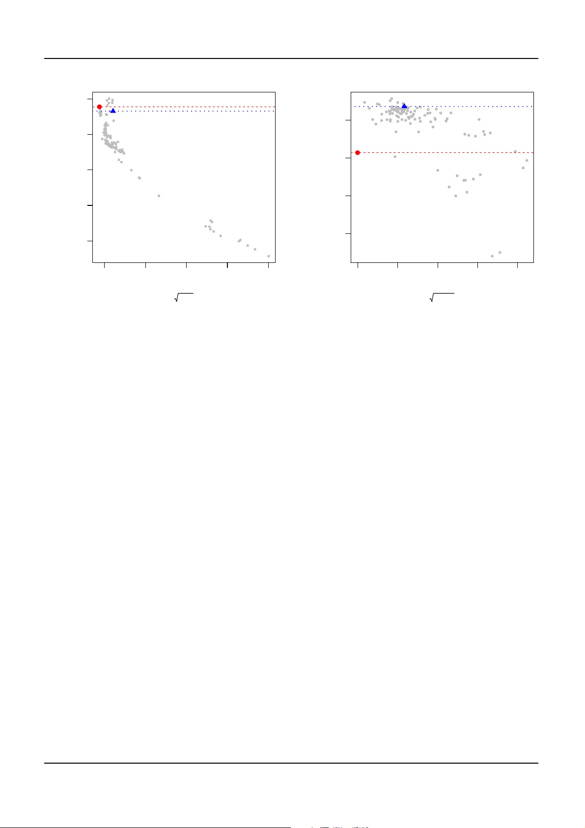
Model Selection via Focuse d Inf ormation Criteria f or Comple x Data in Ecology and Ev olution Gerda Claeskens 1 , C ´ eline Cunen 2 , and Nils Lid Hj o r t 2 , ∗ 1 ORST A T and Leuv en Statistics Research Centre , KU Leuv en, Belgium 2 Depar tment of Mathematics, University of Oslo , Norwa y Correspond ence*: Nils Lid Hjor t nils@math.uio .no ABSTRA CT Datasets encountere d when e xamining deeper issues in ecology and e vo lution are often comple x. This calls f or careful strateg ies f or both mod el b uilding , model selection, an d model a ve ragin g. O ur paper aims at motiva ting, e xhibiting, and fur t her de veloping focuse d model selection cr iteria. In conte xts inv olving precisely fo rmulated interest parame ters, these versio ns of FIC , the f ocused inf ormation c r iterion, ty pically lead to better ﬁnal precision for the most salient estimates, conﬁdence intervals, etc. as compa red to estimator s obtained from other selection methods. Our methods are illustra ted wit h re al case studies in ecology; one rel ated to bird species ab undan ce and another to the decline in body c ondition fo r the Antarctic minke whale. Keyw ords: bird sp ecies a bun dance , ecology , evolution, FIC and AFIC, focused mod el se lection, linear mixed effects, minke wh ales 1 INTRODUCTION Only rarely will initial modelling ef forts lead to ‘one and only one model’ for the data at hand. This simple empirical st at em ent applies in p arti cular to s ituations with complex data for compli cated and not - yet-understood m echanisms u n derlying th e phenomena b eing studied, in ecology and e volution, as well as other sciences. Thu s metho d s for m odel comp arison, mo del selection, and m o del av eraging are called for . Not surprisingly th ere must be se veral su ch method s, sin ce the question ‘what is a good model for my data?’ cannot b e expected to have a simpl e and clear-cut answer . There ar e i ndeed sev eral model selection s chemes in th e s tatistics li terature, with th e m ore famous ones being the AIC (the Akaike Information Criterion) and the BIC (the Bayesian Informatio n Criterion); see Claeskens and Hjort (2008b) for a general overvie w . The AIC and BIC are able to compare and rank competing models for a given dataset, as long as they are all parametric. These and yet other methods work in an ‘ov erall modus’, in appropriate senses comparing overall ﬁt wi th overall complexity , but they do not take on board the i ntended use of the ﬁtted models . This is where FIC (the F ocused Informati on Criterion) comes in, along with certain relativ es. The FIC aims at giving the most relev ant model comparison and ranking, and hence also po inting to the best model, for the given purp o s e . What thi s given purpose i s depends on the scientiﬁc context. Indeed, two research teams might ask differ ent focused questions, with the same data and t he same list of candid ate models, and we judge it not to be a contradiction in t erms that three focused questions m ight ha ve three different best m odels. 1 Claeskens, Cunen, Hjort Focused Inf or mation Criteria The present article give s an account of FIC and its relativ es, includ i ng also certain extensions of pre viously publ ished methods. W e do ha ve models for ecology and ev olution in mind, though it is clear that the view is broader: we wis h to ﬁnd good st atistical models for complex data, and can do so, once crucial and context driven questio n s are translated to focus parameters . Our paper’ s contribution is twofold. (i) W e aim at in troducing the FIC m ethodology to researchers in ecology and ev o l ution. W e ha ve therefore striv ed to include relev ant examples, along wit h some R code. W e also discuss various t o pics of i nterest to appli ed researchers, particularly i n Section 5. In th i s partly tutorial spirit, various technical detail s have been pl aced in the append i x. (ii) Our article also serves as an out let for a somewhat ne w FIC frame work, termed t he ‘ﬁxed w i de m odel frame work’, dif ferent from the ‘local asym p totics framew ork’ used in the majority of previous publicatio n s. Details are in Section 3, with m aterial not been presented in t his g eneral form before. In p arti cular , the extension of this frame work to generalised linear models is nov el. T o help ﬁx ideas and some basic notation, we start with a concrete app l ication. W e use the dataset from Hand et al. (1994) regarding counts of the number of bird species on fourteen areas, vegetation islands, in the Andes mountains with p ´ aramo vegetation. In addition t o the number of bi rd species y , there are four cov ariates recorded for each such vegetation isl and: x 1 , the area of the vegetation island in thou s ands of square kilometers; x 2 , the elev atio n in t housands of meters; x 3 , the distance between the area and Ecuador in kilometers; and x 4 , the distance from t he nearest island in kilometers. y x1 x2 x3 x4 36 0.33 1.26 36 14 30 0.50 1.17 234 13 37 2.03 1.06 543 83 35 0.99 1.90 551 23 11 0.03 0.46 773 45 21 2.17 2.00 801 14 11 0.22 0.70 950 14 13 0.14 0.74 958 5 17 0.05 0.61 995 29 13 0.07 0.66 1065 55 29 1.80 1.50 1167 35 4 0.17 0.75 1182 75 18 0.61 2.28 1238 75 15 0.07 0.55 1380 35 W e model the number of bird species Y by a P oisson distribution with mean exp( x t β ) , where x i n the widest model consists of the con s tant 1 (modelling the intercept), all four cova riates x 1 , . . . , x 4 as main ef fects, and all six pairwise interactions between these m ai n effects. This amounts to a total of 11 parameters β 0 , . . . , β 10 . W e wish to include the intercept parameter β 0 in all candid ate m odels, and hence take it as a ‘protected parameter’, whereas the ot her parameters are ‘open’, and can b e pushed in and out of candidate mo d els. For this application, all submodels of the largest 11-parameter model are considered, with the further restriction t hat interactions between t wo covariates can be inclu ded only if the two main ef fects are present. This results i n a total of 11 3 models. The main di stinction between FIC and various other information criteria is the presence of a focus . This is a quanti ty of int erest that depends on the model parameters and is estimable from the data. The generic notation for the focus used in our paper is µ . Its dependence on the m odel parameters mi g h t be indi cated by writing µ ( β ) . This is a provisional ﬁle, n ot the ﬁnal typeset ar ticle 2 Claeskens, Cunen, Hjort Focused Inf or mation Criteria In the bird species study , our ﬁrst focus concerns one of the vegetation islands, Chiles. This area is the one among the fourteen that is closest to Ecuador , and has cov ariate values x 1 = 0 . 33 , x 2 = 1 . 26 , x 3 = 36 , x 4 = 14 . W e wish to select a m o del that b est estimates th e expected number of bird species for this island, that is, µ ( β ) = exp( x t β ) for the given covar iate values for Chiles. In our m odel search problem there are 113 models and hence 1 1 3 estimators for µ . Each s uch estimator , s ay b µ M for a candidate model M , comes with i t s own bias and variance, say b M and τ 2 M . Thus, for each candidate mod el there is a corresponding mean squared error (mse) mse M = τ 2 M + b 2 M . (1) The basic id ea of the FIC is to estimate these mse values from the d at a, for the wide as well as for each candidate model, i.e. to cons truct FIC M = d mse M = b τ 2 M + d bsq M , (2) with th e second term indicating estimation of the squared bias bsq M = b 2 M . In the end one s el ects the model with the s mallest estimated mse. For th e bi rd species application, we use FIC for ﬁnding the best mo del to est i mate the expected number of bird species for Chiles. W e us e t he R package fic with the fol lowing lines of R code, where we ﬁt the wide model, specify t he focus function, the cova riate value in which t o ev aluate this focus, and the s peciﬁc models that we wish t o search th rough. In thi s example we restrict the built-in all subsets sp eciﬁcation t o only us ing models that obey the hierarchy principle (so out of the 2 10 = 1024 potent i al subm odels, only the 113 pointed t o above are included). library(fi c) wide.birds = glm(y ˜ .ˆ2, data=birds, family=poiss on) focus1 = function(p ar, X) exp(X % * % par) inds0 = c(1,rep(0,1 0)) # only the intercept is in the narrow model A = all_inds(w ide.birds, inds0) # use all subsets of the wide model #exclude models with interaction s that do not have both main effects: inds <- with(A,A[!( A[,2]==0 & (A[,6]==1|A [,7]==1|A[ ,8]==1) | A[,3]==0 & (A[,6]==1|A[ ,9]==1|A[, 10]==1) | A[,4]==0 & (A[,7]==1|A[ ,9]==1|A[, 11]==1) | A[,5]==0 & (A[,8]==1|A[ ,10]==1|A[ ,11]==1)), ]) # specify the X used to evaluate the focus function: XChiles=mo del.matrix (wide.birds)[1, ] fic(wide=w ide.birds, inds=inds, inds0=inds0, focus=foc us1, X =XChiles) For each of the 113 models we g et vi a the o utput values of t h e focus estimat e, the esti m ated bias, standard error , and actually two versions of t he FIC of (2), corresponding to two related b ut diff erent ways of estimating the b 2 M part (for d etai l s, see Section 2). For FIC tables and FIC plot s we prefer working wit h the square-root of the FIC, i.e. est imates of the root-ms e (rmse) rather than o f th e m se, as these are on the original scale of t h e focus and easier to i nterpret. T able 1 is constructed from the output for a selection of mo dels, incl u d ing the narrow model (1) which has a relati vely large (in abs o lute value) bias esti mate of − 19 . 035 , a relati vely small standard error of 2.247 and a focus estimate of 20. 7 1 ; the wide model (113) with zero as the bias estimate t hough wi t h a Frontiers 3 Claeskens, Cunen, Hjort Focused Inf or mation Criteria lar ge standard error of 6.051. This is a typical output: the wide mod el contains 11 parameters t o estimate which causes the st and ard error t o b e large, t h e narrow model only cont ains the intercept resultin g i n a small s tandard error . For the bi as estim ate the scenario is rever sed: the wide mod el has the smallest bias, while the narrow model has a larger bias. The balancing act of the FIC via the mean squared error ﬁnds a compromise. The selected m odel (5) results in t he smallest value of the s quare root of the estimated mean squared error (rmse). Its indicator sequence 10010,000000, with a one for β 0 and β 3 , and zeroes for the interactions, points towards the selected focus µ ( β ) = exp( β 0 + β 3 x 3 ) with corresponding estim ated focus value 38.88. Using the wide model would have resulted in a close 38.27 t hough with a larger estimated root mean squared error . The wide mod el only ranks at the 73rd place according to estimated rmse. M odel (20) is selected by the Bayesian information criterion BIC, it consists of the in t ercept, all four main eff ects and the interaction between x 1 and x 2 . In the rms e rankin g it comes at the 42nd pl ace. Model (67 ) is the one sel ected by the Akai ke information criterion, next to the i ntercept and all main ef fects it consists of the interactions x 1 x 3 , x 2 x 3 , x 2 x 4 . This m odels ranks 32nd. T able 1. Bird species example. This t able is con s tructed from output of t he R function ﬁc for six of the 113 models, together with the AIC and BIC values. FIC selection takes place via the square root of the estimated mean squared error of th e focus estimator . model coef. indicators focus bias se √ FIC AIC BIC 1 10000,000000 20.714 − 19.035 2.247 19.167 143.26 143.90 5 10010,000000 38.882 0.000 4.383 4.383 112.65 113.93 20 11111,100000 33.718 − 2.156 4.670 5.143 91.91 95.74 28 11101,001000 26.356 − 11.0468 3.674 11.642 98.54 101.74 67 11111,010110 39.784 0.000 5.296 5.296 91.44 96.55 113 11 1 11,111111 38.269 0.000 6.051 6.051 95.72 102.75 The second focus con cerns the probabilit y of ha ving more th an 30 bird species, Pr( Y > 30 | x ) . Now we do not sp ecify a particular i s land b ut use th e average FIC (see Section 2.2), wi th equal weights for th e fourteen vege tation islands (non-equal weig h ts can easily be work ed with too). focus2 = function(p ar, X) 1-ppois(30 ,lambda=ex p(X % * % par)) Xall = model.matrix (wide.bird s) fic2 = fic(wide=wid e.birds,in ds=inds,inds0=inds0,focus=focus2,X=Xall) AVE = fic2[fic2$val s=="ave",] which.min( AVE$rmse.a dj) The AFIC selects t h e fol lowing form for t h e mean: exp( β 0 + β 1 x 1 + β 2 x 2 + β 4 x 4 + β 7 x 1 x 4 ) . The av eraged focus estimat e of the probabil ity of observing over 30 bird species in the selected m o del equals 15.73%, while th e wide model’ s estimate is 21.83%, t h ough with a substanti al larger estimated mean squared error due to the estimation o f 11 parameters instead o f onl y 5 for t h e selected model. Of cours e, AIC and BIC ignore any informat i on regarding the focus, and thus s t ill recommend the very same m o dels, mod el (67 ) for AIC, with estimate 21. 1 5 %, and model (20) for BIC, wi th estimate 21.59%. The A IC mo del ranks 16th, the BIC model is no w at t he third place. Figure 1 displays for these two foci the root-FIC and root-AFIC v alues, as well as the estimated focus values, for all of t he 113 models. The FIC or AFIC selected v alues, mini m ising the respectiv e criteria, are indicated in red, w h ile the wide model’ s values are in blue. This is a provisional ﬁle, n ot the ﬁnal typeset ar ticle 4 Claeskens, Cunen, Hjort Focused Inf or mation Criteria (a) (b) 5 10 15 20 25 20 25 30 35 40 FIC Estimated f ocus 1 0.10 0.15 0.20 0.25 0.30 0.05 0.10 0.15 0.20 AFIC Estimated f ocus 2 Figure 1. The two plots gi ve values for a total of 113 Poisson regression m odels, related to two different focused question s. (a) FIC plot for estim ating t he expected num b er of bird species for the Chiles region. (b) AFIC plot for estimating the probabilit y o f observing over 30 species, ave raging over all 14 isl ands. The red do t and line indicate the selected v alue, the blue tri ang le and line are for th e wi de model. Se veral tradi t ional model selection criteria, such as the AIC and the BIC (see Claeskens and Hjort, 2008b, Chs. 2, 3) work in an overall modus, ﬁnding models that in a statis t ical sense are goo d o n a verage, no t taking on board the speciﬁc aims of a stud y . The FIC works explicitly with such speciﬁc aims , formalised via the focus parameters. Thus FIC mig ht ﬁnd that one m odel works very well for covariates ‘in the middle’, whereas another mo d el could work rather b etter for cova riates outside m ainstream. Similarly , one mod el might work well for explaining m eans, and another for explaining variances. W e stress that the FIC apparatus works for any speciﬁed fo cus parameter , and is not limi t ed to e.g. regression coef ﬁcients and the customary selection o f cov ariates from that perspective . The generic FIC formula (2) cannot be immediately applied, as ef forts are required to establish formulae for approximations to biases and var iances, along wit h construction of estimators for these quantities. Thus the FIC formula pans out differently in di ff erent situations , depending on th e g eneral frame work, the complexity of m odels, and estimators of the focus parameters. A brief overvie w of general principles, leading to such approxim ations and estimators, is given in Section 2. This also encompas s es AFIC, ways of creating a verage-FIC scores in situation s where more than one focus parameter is at st ake. In Section 3 we provide t he g eneral FIC formulae in t he so -called ﬁxed wide m odel frame work. The dev elopment of FIC formulae ingredients in a somewhat different framework, with local neig bourhood models, is placed in Section 6. Generalised linear models are used as exa mples, encompassin g linear regression, lo gistic and Poisson regression, etc. The more general class of linear mixed models has p roven important for various applications to ecology , and in Section 3.3 FIC formulae are reached for such. In Section 4 we use linear mixed ef fects models wi th FIC for analysing the body cond itions of minke whales in the Antarctic, where one focus parameter is the yearly decline in ener g y storage. A general b ut brief discussion i s th en offered in Section 5. Here we touch on aspects of performance, along with a fe w concluding remarks, some o f which point to future research. Frontiers 5 Claeskens, Cunen, Hjort Focused Inf or mation Criteria 2 FOCUSED IN FOR M A TION CRITERIA The application concerning bi rds on vegetation isl ands in the previous secti o n was meant to provide intuition for the use of FIC for model selection . Here we giv e a more formal, but brief, overvie w of the FIC and AFIC schemes. 2.1 General FIC sc heme Suppose we ha ve deﬁned a wide model whi ch is assumed to be the true data-generating mechanism. Estimating the focus parameter using the wide m o del leads t o b µ wide , which under broad regularity conditions w i ll aim at µ true , the unknown true value of the focus parameter . Estim ation via ﬁtting a candidate model M leads to b µ M , say , aiming for some l east false parameter µ 0 ,M , t y pically d iffe rent from µ true , due t o mod el l ing bias. The least false parameter in question relates to the best approx imation candidate model M can manage to be, to the true model. There is therefore an inherent bias, say b M = µ 0 ,M − µ true , associated wit h using M . W e saw estimates of this bias in the birds application above, where sm all m o dels could ha ve larger biases. The esti mators will h ave certain variances. In most framew orks, in v olving i ndependent or weakly dependent data, t hese tend t o zer o with speed 1 /n , in terms of growing sample size n . It is therefore con venient and informative to write these var iances as τ 2 wide = σ 2 wide /n and τ 2 M = σ 2 M /n , where the m athematics and approximation theorems associat ed with different frameworks typically yield expressions for or approximati o ns to the σ wide and σ M . The mse of the focus parameter estimators is the sum of the v ariance and the bias sq uared, mse wide = σ 2 wide /n + 0 2 and mse M = σ 2 M /n + b 2 M . (3) These quanti t ies are measures of the risk , in the statis t ical sense, asso ci at ed with using each of the models for estimatin g µ . As explained i n the introduct i ons, the FIC scores of (2) are estim ates of the mse of t he focus parameter est imators, i.e. the b µ M , for a speciﬁc dataset, for each of the m odels u nder consideration. Eq. (3) is also an inform ativ e reminder t h at with more data, v ariances get small, b ut biases remain. So using a m odel which i s not full y correct can s t ill yield sh arper estimators, as long as t he bias is moderate or small: | b M | < ( σ 2 wide − σ 2 M ) 1 / 2 / √ n . It is also clear that wit h steadily m ore data, steadily m ore sophisticated models can and indeed s hould be used. The FIC makes these ideas operativ e. In various cases t he variance terms σ 2 M /n are easier to estim ate than the squ ared biases b 2 M . A st arti ng point for th e latter i s b b M = b µ M − b µ wide , but the correspondin g b b 2 M will overshoot b 2 M with abou t κ 2 M /n , which is the variance of b b M . W ith appropriately constructed est i mators of the quantiti es σ wide , σ M , κ M (with differe nt recipes for different sit uations), t his yields two natural ways of estimating the actual mse values: FIC u wide = b σ 2 wide /n + 0 2 and FIC u M = b σ 2 M /n + b b 2 M − b κ 2 M /n, FIC wide = b σ 2 wide /n + 0 2 and FIC M = b σ 2 M /n + max( b b 2 M − b κ 2 M /n, 0) . (4) The FIC u scores are (approximately) un b iased estimates of th e mse , since b b 2 M − b κ 2 M /n is (approxi mately) unbiased for b 2 M , wh ereas the FIC scores are adjust ed versions, by t runcating any negative estimates of squared bias to zero, as we did in the ﬁrst example. If the true bias in question is som e distance away from This is a provisional ﬁle, n ot the ﬁnal typeset ar ticle 6 Claeskens, Cunen, Hjort Focused Inf or mation Criteria zero, FIC u M will be equal to FIC M . When faced with a sp eciﬁc application one s hould d ecide on on e of these two FIC versions, and use t he same choice for all models under consideration. In order to turn the general scheme (4) into clear formulae, with consequent algori t hms, we need expressions for or approximations to the populati o n quantities σ M , b M , κ M , followed by clear esti mation strategies for these again. In mo s t cases we need to rely on large-sample approximations. Arriving at clear formulae for σ M etc. d epends on t he particulariti es of the wide model, the candidat e models, and the focus parameter . W e provide such FIC formul ae, for two differ ent frame works or setups. The ﬁrst in volve s local asymptotics, with candidate models being a local distance O (1 / √ n ) away from th e wide mo del. Thi s deriv ation is placed in Section 6. The second av oids such lo cal asymptot ics and works from a ﬁxed wide model and a col lection of candidate models , see Section 3. It is not a contradict i on in terms that these two frame works lead to related but not identical FIC formulae, as diffe rent mathematical approximati ons are at work. 2.2 AFI C, the av eraged-weighted selection scheme The FIC apparatus above is tailored to one speciﬁc focus parameter at a ti me. In a regre ssion context this applies e.g. to estimati n g the mean response function for one covariate vector at a time, say µ ( θ ; x 0 ) . Often there would be acti ve interest in se veral parameters, howe ver , as wi t h such a µ ( θ ; x 0 ) for all x 0 in a segment of cova riates, or a probability Pr( Y ≥ y 0 | x 0 ) for a set of thresholds, as in th e bi rds study . Suppose in general that an ensemble of estim ands i s of interest, say µ ( θ ; v ) with v ∈ V , and that a measure of r elativ e importance d W ( v ) is assigned to t hese. There coul d be only a fe w such estim ands under scrutiny , say µ j for j = 1 , . . . , k , alo ng with weight s of importance w 1 , . . . , w k . Estimat i on in volving all hi gher quantiles, or all cov ariates within a certain region, howe ver , would constitute examples where we need the more general v ∈ V notation. Here we sketch th e AFIC approach, for estimating the rele vant integrated weighted risk. For each focus parameter in the ensemble of estimands th ere is an associated mse or risk, mse( v ) . Th e combined risk associated with us ing model M then becomes r n ( M ) = Z mse( v ) d W ( v ) = Z { σ M ( v ) 2 /n + b M ( v ) 2 } d W ( v ) , with the appropriate σ M ( v ) and b M ( v ) = µ 0 ,M ,n ( v ) − µ true ( v ) . An approximately unbiased estimate of this combined risk is aﬁc u ( M ) = Z { b σ M ( v ) 2 /n } d W ( v ) + Z { b b M ( v ) 2 − b κ M ( v ) 2 /n } d W ( v ) . This is the same as a direct weighted sum or integral of the individual FIC u ( M , v ) scores. The adjus ted version, h owev er , where a potentially negative value of the estimated integrated squared bias is being truncated to zero, is no t identical to the integral of the FIC( M , v ) scores. It is rather equal to aﬁc( M ) = Z { b σ M ( v ) 2 /n } d W ( v ) + max h Z { b b M ( v ) 2 − b κ M ( v ) 2 /n } d W ( v ) , 0 i . As with FIC, there are two related, but not identical, approximation schemes, t he ﬁxe d wide m odel setup and the local asymptot ics, of respectiv ely Section 3.1 and Section 6.1, leading now to somewhat dif ferent AFIC formulae. For details and applications, see Claeskens and Hjort (2008b, Ch. 6), Claeskens and Hjort (2008a). Frontiers 7 Claeskens, Cunen, Hjort Focused Inf or mation Criteria There is a connection between Akaike’ s information criterion AIC and AFIC wit h certain mo del dependent weights, see Claeskens and Hj o rt (2008a, Sec. 6.2). Broadly speaking, the AIC t urns out to be lar ge-sample equiv alent to cases with AFIC where ‘all things are equally important’. 3 FIC WITHIN A FIXED WIDE MODE L FRAMEWORK The FIC as used in the bird species example is the version as deriv ed in Claeskens and Hjort (2003), see also Claeskens and Hjort (2008b, Ch. 6). For the estimation of bias and variance a local asymptoti c frame work is used in which t h e parameters of the true densi ty of t he data are assumed to be of t he form γ = γ 0 + δ / √ n , with n the s am ple size, see Section 6 for mo re explanation. Th is assum ptions means in practice that we belie ve that all models are relativ e c lose to each other and to the truth. Moreover , all m odels are s u bmodels of a wid e m o del. Since the deriv at i on of the FIC formulae i s contained in t h e references above , we o nly place a summary in th e appendi x. In this section we p resent t he ‘ﬁxed wide model’ frame work, which is particularly us eful if the set of candidate mo d els are seen as not being in a reasonable vicinity of each other . This s econd frame work allows candidate models o f a different sort from the wide model; in parti cul ar , a candidate m o del does not hav e to be a clear submodel of th e wide m odel. Keep in min d that the two di fferent FIC frame works hav e t he same aims and mo tiv ati on; the difference between them lie in the d i ff erent mathematical tools for estimating the rele v ant ms e quantit ies, which lead to dif ferent formulae. In the discussi on section 5 we come back t o some differe nces between the t wo frame works. Here we start i n Subs ection 3.1 by presenting the ﬁx ed wide model FIC in a general regression setup. Then in t he two foll owing subsections we deal wit h two speciﬁc m odel classes of general interest, generalised linear models and linear mixed models, in more d et ai l . 3.1 General regression models In this subsection we use the familiar ( x i , y i ) n o tation for the regression data, with x i the cov ariate vector in question. The FIC machinery we develop here starts from the existence of a ﬁxed wide model. The dev elopment represents an extension of earlier work o f Jullum and Hjort (2017, 2019) for i.i.d . data and surviva l analy sis, Ko, Hjort, and Hobæk Haf f (2019) for copu lae model s , Cunen, Hjort, and Nyg ˚ ard (2019a) for po wer-law distributions (with applications to war and conﬂict data) and Cunen, W alløe, and Hj ort (2019c,b) for l inear m ixed eff ects models (wi th application to whale ecology). Since we wish t o estimate the mse of the focus estimato r in different models, we ﬁrst cons ider the asymptotic distribution of the parameter estimator in the wide model and ne xt in the other models of interest. The distributions are used to form the mse’ s o f th e focus estimators and ﬁnally we const ruct the ﬁc as an estimated mse and sel ect th e m odel with the smallest ﬁc v alue. Suppose a wide model density is agreed upon, of the form f ( y i | x i , θ ) , for a certain parameter vector θ , of length p . W e consid er this t o b e the true mod el. This θ would typically encompass bot h regression coef ﬁcients and parameters related t o the spread and shape of error distributions. W ith u ( y i | x i , θ ) = ∂ log f ( y i | x i , θ ) /∂ θ the score function, and J n = n − 1 P n i =1 V ar wide u ( Y i | x i , θ true ) th e normalised Fisher information m atrix at t he true parameter . Under m ild regularity conditions we ha ve the following well-known result for the maximum likelihood esti m ator b θ wide , √ n ( b θ wide − θ true ) ≈ d N p (0 , J − 1 n ) . (5) This is a provisional ﬁle, n ot the ﬁnal typeset ar ticle 8 Claeskens, Cunen, Hjort Focused Inf or mation Criteria The notation in dicates approxi m ate mul tinormality to the ﬁrst order as the sample size grows, and can also be supplemented with a clear limit distribution statem ent, in that case in volving a li mit cov ariance matrix J for J n . Cons i der now a candi d ate m odel M , di f ferent from the wi de one, p erhaps also in structure and form. W ith notation f M ( y i | x i , θ M ) for its density , and u M ( y | x i , θ M ) for its score function, we ha ve a maximum likelihood estimator b θ M , of l ength p M , maxim ising the log -l ikelihood function ℓ n,M ( θ M ) = P n i =1 log f M ( y i | x i , θ M ) . If the wide m odel is considered to be the trut h, the estim ator in model M does not necessarily aim at the true parameter , b ut at the least false p arameter θ 0 ,M ,n , which is the minim iser of the Kullback–Leibl er di s tance from the data-generating mechanism to the model; see details i n Section 6.3. The estimator in the candidate mo del has a limiting m u ltinormal distribution, with a sandwich type var iance matrix, √ n ( b θ M − θ 0 ,M ,n ) ≈ d N p M (0 , J − 1 M ,n K M ,n J − 1 M ,n ) , (6) where J M ,n = − n − 1 n X i =1 E wide ∂ 2 log f ( Y i | x i , θ 0 ,M ,n ) ∂ θ M ∂ θ t M and K M ,n = n − 1 n X i =1 V ar wide u M ( Y i | x i , θ 0 ,M ,n ) . The v ariance m atrices here are deﬁned with respect to th e wi d e m odel, at position θ true . From approx i mations (5)–(6) the del t a method may be called upon to read off relev ant expressions for the approximate dist ributions of t he focus parameter estimato rs b µ wide = µ ( θ ) and b µ M = µ M ( θ M ) , where the latter is aim ing for the l east false parameter value µ 0 ,M ,n = µ M ( θ 0 ,M ,n ) associated with model M . Crucially , we also need a mul tinormal approxi mation to the joint distribution of ( b µ wide , b µ M ) , in order to assess the distribution of the bias estimator b b M = b µ M − b µ wide ; wit h out that part we can’ t b uild an appropriate estimator for b 2 M . In the appendix, Section 6.3, we go through such arguments, and reach  √ n ( b µ wide − µ true ) √ n ( b µ M − µ 0 ,M ,n )  ≈ d N 2 (0 , Σ M ,n ) . (7) Here th e 2 × 2 matrix Σ M ,n has diagon al terms c t J − 1 n c and c t M ,n J − 1 M ,n K M ,n J − 1 M ,n c M ,n , with gradi ent vectors c = ∂ µ ( θ true ) /∂ θ and c M ,n = ∂ µ ( θ 0 ,M ,n ) /∂ θ M of lengths p and p M . The of f-diagonal term of Σ M ,n takes the form c t J − 1 n C M ,n J − 1 M ,n c M ,n , with a formu l a for the required covariance related term C M ,n in the appendix. From (7) we can read of f mse approximations, mse wide . = c t J − 1 n c/n + 0 2 and mse M . = c t M ,n J − 1 M ,n K M ,n J − 1 M ,n c M ,n + b 2 M , with bias b M = µ 0 ,M ,n − µ true . For the latter we us e the estimator b b M = b µ M − b µ wide , where the result above also leads to a clear approximation for the di s tribution o f √ n ( b b M − b M ) . This leads to FIC formulae, unbiased and adj usted, as FIC u wide = b c t b J − 1 n b c/n + 0 2 and FIC u M = b c t M b J − 1 M b K M b J − 1 M b c M /n + b b 2 M − b κ 2 M /n, FIC wide = b c t b J − 1 n b c/n + 0 2 and FIC M = b c t M b J − 1 M b K M b J − 1 M b c M /n + max( b b 2 M − b κ 2 M /n, 0) . (8) Frontiers 9 Claeskens, Cunen, Hjort Focused Inf or mation Criteria Here b c and b c M emer ge by computing gradients of µ ( θ ) and µ M ( θ M ) at their respecti ve maximum likelihood positi o ns, and b J n , b J M are com puted as norm al i sed observed Fisher informatio n matrices, for the wide and for the candidate m odel in question; speciﬁcally , b J M is 1 /n times minus the Hessian m atrix from the lo g-likelihood, − ∂ 2 ℓ n,M ( b θ M ) /∂ θ M ∂ θ t M . Also, the p M × p M matrix b K M is n − 1 P n i =1 b u M ,i b u t M ,i , with b u M ,i = u M ( y i | x i , b θ M ) . Finally , the b κ 2 M /n estimat es in v olves also t he p × p M matrix b C M , which is n − 1 P n i =1 b u wide ,i b u t M ,i . M odel selection p roceeds by com puting FIC M , t h e esti m ated mse of the focus estimator b µ M , for all models M of interest, and t hen selecting that mod el for which this score is t he lowest. 3.2 FIC for g eneralised li near mo d els, with a ﬁxed w ide model W e i l lustrate this FIC machinery for one popular cl ass of generalised linear models, n am ely the Poisson regression mo d els. Generalisations to other generalised linear models are relatively imm ediate. Suppose therefore that we have cou n t data y i along wi t h a cov ariate vector x i of length p . F or the ﬁxe d wide model we take the Pois son regression m odel wit h y i ∼ Pois( ξ i ) , with ξ i = exp( x t i β ) containing all covariate information; in particul ar , there is also a true parameter β true there. Cons ider then an alternative candidate model M wh ich inst ead takes the means t o be ξ M ,i = exp( x t M ,i β M ) , with x M ,i of l eng th p M , perhaps a subset of the full x i , or perhaps with some entirely other pieces of cov ariate information. Here the log-densities take t h e form − ξ i + y i log ξ i − log ( y i !) , which means log f = − exp( x t i β ) + y i x t i β − log ( y i !) and log f M = − exp( x t M ,i β M ) + y i x t M ,i β M − log ( y i !) , for the wide model and the candidate mo del, along w i th score functions u ( y i | x i , β ) = { y i − exp( x t i β ) } x i and u M ( y i | x M ,i , β M ) = { y i − exp( x t M ,i β M ) } x M ,i . From this we d edu ce J n = n − 1 n X i =1 exp( x t i β true ) x i x t i , J M ,n = n − 1 n X i =1 exp( x t M ,i β 0 ,M ,n ) x M ,i x t M ,i , K M ,n = n − 1 n X i =1 exp( x t i β true ) x M ,i x t M ,i , along with the p × p M cov ariance matrix C M ,n , deﬁned as n − 1 n X i =1 E wide { Y i − exp( x t i β true ) } x i { Y i − exp( x t M ,i β 0 ,M ,n ) } x t M ,i = n − 1 n X i =1 exp( x t i β true ) x i x t M ,i . Consistent estimates of these popul ation matrices are obtain ed by ins erti ng b β wide for β true and b β M for β 0 ,M ,n . Notably , as long as there is a well-deﬁned wide Poisson regression model, as assumed here, th e frame work is sufﬁ ciently ﬂexible and broad to encomp ass also non-Poisson candidate models. Using the FIC apparatus in v olves working with l o g-likelihood functions and score functions for these alternative This is a provisional ﬁle, n ot the ﬁnal typeset ar ticle 10 Claeskens, Cunen, Hjort Focused Inf or mation Criteria models, leading t o different but workable expressions for the m atrices J M ,n , K M ,n , C M ,n above. The stretched Poisson m odels us ed in Schweder and Hjort (2016, Exercise 8.18) are a case in point ; t hese allow both ov er - and u nderdispersion. 3.3 FIC for l inear mixed effec ts models Models with random eff ects, often called m i xed effect models, are widely used i n ecological applications. In Cunen, W alløe, and Hj ort (2019c) FIC formulae have been de veloped for the class of linear mi xed effec t models (often abbre viated LM E m odels). Here we wil l giv e a brief descripti o n of that approach, which also serv es as a special case of the general FIC approach for a ﬁxed wide model framework, see (8). Generalisations to classes of n o nlinear mixed effe ct models, and also to heteroscedastic si t uations where variance parameters depend on covariates, can be foreseen, following similar chains of ar guments b ut in volving m ore elaborations. Suppose w e hav e n observations of y i , a vector of length m i . The m i datapoints withi n each y i vector are assumed to be dependent, and will often correspond to data collected in t he same space or time. Here we wil l refer to t hese data as belong i ng to the same gr oup . Each y i vector is ass ociated wi th a regressor matrix X i of dimens i on m i × p for the ﬁxed effects, and a design matrix Z i of dimens i on m i × k for the random ef fects. The linear m i xed effects m odel takes the form y i = X i β + Z i b i + ε i for i = 1 , . . . , n, with the b i ∼ N k (0 , D ) independent of th e errors ε i ∼ N m i (0 , σ 2 I m i ) . The model may also be represented as Y i ∼ N m i ( X i β , σ 2 ( I m i + Z i D Z t i )) , (9) and its parameters are θ = ( β , σ, D ) . Note that th e ordinary li near regression mo del is a special case, corresponding to D = 0 . The log-likelihood cont ribution for this group of the data may be written ℓ i ( θ ) = − m i log σ − 1 2 log | I m i + Z i D Z t i | − 1 2 (1 /σ 2 )( y i − X i β ) t ( I m i + Z i D Z t i ) − 1 ( y i − X i β ) . The comb ined log-li kelihoo d P n i =1 ℓ i ( θ ) leads to maxim um likelihoo d est i mators and hence also to b µ wide = µ ( b β wide , b σ wide , b D wide ) for any focus parameter µ = µ ( β , σ, D ) of interest. In applied situat i ons we will spend efforts and call on b i ological knowledge to con s truct a well-motivated wide model, of the form (9). This wide model will t y pically be based on our kn owledge of the system under study and, crucially , on ho w t he data were collected. Quite often the resulting model cou l d become big , in the sense that it includes a l ar ge nu m ber p of ﬁxed ef fects and also a large nu m ber k of random ef fects. As sume, as we do t hroughout this paper , that our primary i n terest lies i n the precise estim ation o f some focus parameter µ , wh ich could be a function of the ﬁxed effect coefﬁcients β , and/or the variance components ( σ , D ) . For such a µ = µ ( β , σ , D ) , can we ﬁnd ano t her model which offers mo re precise estimates of µ than b µ wide = µ ( b β wide , b σ wide , b D wide ) implied by the wide model? FIC answers the question above; we can search among a set of candidate models for one giving mo re precise estimates of µ . In the sim p l est setti ng, the candidate mo del is deﬁned with respect to the same n groups as in the wide m o del in (9), and we write y i ∼ N m i  X M ,i β M , σ 2 M ( I + Z M ,i D M Z t M ,i )  . Frontiers 11 Claeskens, Cunen, Hjort Focused Inf or mation Criteria This m odel h as desi gn m at ri ces, X M ,i and Z M ,i , potential l y different from those of the wide mod el, and hence also a different set of parameters, say θ M = ( β M , σ M , D M ) . Often, but not necessarily , the candidate model wi l l in volve subsets of t he covariates (i.e. columns ) included in X i and Z i , respectively . Let the cov ariate matrix X M ,i hav e dimension m i × p M , and Z M ,i being m i × k M . The focus parameter must then be represented properly inside the candidate model, as µ M = µ M ( β M , σ M , D M ) , leading to the estimate b µ M = µ M ( b β M , b σ M , b D M ) . In order to work out FIC form ulae, we ﬁrst need to study t he joint large-sample beha viour of the estimator from t he wide model b µ wide and the estimator from the ca ndidate m odel b µ M . This is as with eq. (7) in Section 3.1, but the current framew ork i s more complicated and needs further efforts. Such work is carried out in Cunen, W all øe, and Hjort (2019c), and l ead to  √ n ( b µ wide − µ true ) √ n ( b µ M − µ 0 ,M ,n )  ≈ d N 2 (0 , Σ M ,n ) , with all quantities deﬁned analogously to what is presented in Section 3 .1. These inclu d e matrices J n , J M ,n , K M ,n , C M ,n and g radi ent vectors c and c M ,n , deﬁned si milarly to those in Section 3.1, but here in volving more compl icated details than for the plain er regression models work ed with there. This work then yields the same type of FIC form ulae as for eq. (8), b ut with other recipes and formulae for the required estimators for the quantities m ent ioned. Regarding estimators for t he m atrices in v olved, we ha ve t hree general possibil ities: (i) working out explicit form ulae and plug in the necessary parameter estimates; (ii) comput ing the m atrices numerically , in volving certain n umerical integration detail s; (iii) via boots trapping from the estim ated wide mod el . In Cunen, W allø e, and Hjort (2019c) the ﬁrst option is pursued, inv olvi ng lengthy deri va tions of log-dens i ty deriv atives and thei r means, variances, cova riances, computed under the wide model. The resulting formulae are too long for this re vie w , but are fast to compute. Options (ii) and (iii) have yet to be fully in vestigated, but wi ll likely be fruitful when extending this FIC app roach to the wider class of generalised li near mixed m o d els (the so-called GLM Ms). The approach described here w i ll be illus trated in Section 4, but we ﬁrst off er some comments of a more general n at u re. Readers familiar with li near m ixed ef fects m o dels wil l be aware that th ere are two different estimation schemes for models of t h is class, full maxim u m li kelihood and so-called REML estimators, for restricted or residual m aximum likelihood. The REML m ethod takes th e esti mation of t he ﬁxed effects of the model into account when producing estim ators of the variance p arameters. For the compu t ation of FIC scores t h e user m i ght employ either maxim u m likelihood or residual m axi mum likelihood estim at es, since these are lar ge-sample equiv alent ; see for instance Demidenko (2013, Ch. 3). As with the general FIC formu lae (8) there are two versions, the app rox imately un biased estim ates of risks and the adjusted ones. In Cunen, W alløe, and Hj o rt (2019c) it is ar gu ed t hat the unbiased ver sion FIC u M = b c t M b J − 1 M b K M b J − 1 M b c M /n + b b 2 M − b κ 2 M /n (10) tends to w ork best for linear mixed effe cts models. The beneﬁt of this ver sion is that good candid at e models with small biases earn more, com p ared to the wide mo del. In vestigations s how that the FIC formulae of (10) work well, in the s ens e th at they accurately estimate the ris k associated with th e us e of the different candidate models. The FIC formulae are based on large- sample ar gu m ents, which for the case of t h e li near mi xed ef fects models i n volves appro x i mations to normali ty when the number n of g rou ps increases to in ﬁnity . These normal approximations work well as long as the full sample s ize P n i =1 m i grows, particularly for functions of t he linear m ean parameters. M ore care is s ometimes required when This is a provisional ﬁle, n ot the ﬁnal typeset ar ticle 12 Claeskens, Cunen, Hjort Focused Inf or mation Criteria it comes to appl ications in volving non-l i near functions of both mean and v ariance parameters, as with estimates of probabilities µ = Pr( Y ≥ y 0 | x 0 , z 0 ) . 4 APPLICA T ION : THE SLIMMING OF MINKE WHALES Our second application story concerns the potential change in body cond ition of Antarctic minke whales over a period of 18 years. For a more thorough i n vestigation consult Cunen, W alløe, and Hjort (201 9 b). Questions treated there h ave been d iscussed in the Scientiﬁc com m ittee o f the Internatio nal Whalin g Commission (IWC) for a number of years, and a full consensus has not been reached. In th e context of this revie w , therefore, t he analysis below should be taken as an illustration , and not necessarily t he last word on th e to pic of the decline in energy storage or body cond ition for the minke whales. Using data from the Japanese Whale Research Program under Special Permit in the Antarctic (the so- called J ARP A-1) we ha ve studied th e e volution of fat weight in Antarctic minke whales caught in 18 consecutiv e years, from 1988 and 2005. The m ai n biol ogical int erest l i es i n whether or not the wh ales experienced a decline in body condit ion during the study period, and the dis s ected fat wei g h t (in tonnes or kg) is taken to be a prox y for this body con dition. Thus, there is a clear focus parameter in t his application: the yearly decline in fat weight (which we will parametrise in a suitable fashion in t h e following). The whales caught in each year are une venly sampled wi th respect to a number of covariates, for instance sex, body leng th, age, and l ongitudin al region in th e An tarctic ocean. Since all these cov ariates may inﬂuence bod y condit ion we need to include t hem in a model aimi n g at estim ating the potential yearly decline in the respons e. Based on lengthy and detail ed discussions in the Scientiﬁc Committee of t he IWC, we hav e chosen a wide model wi t hin the class of linear mixed ef fect models , see Section 3 . 3 . In Cunen, W alløe, and Hjort (2019b) we have used consi d erable efforts to motivate the choice of covariates, interactions, and random ef fect terms in the wide model, but these arguments are outside the scope of the present article. In R-package-type notation, t he wide model can be given as fatweight ∼ year + year 2 + bodylength + sex + diatom + date + date 2 + age + sex ∗ diatom + diatom ∗ date + diatom ∗ date 2 + bodylength ∗ sex + bodylength ∗ date + bodyle ngth ∗ date 2 + sex ∗ date + sex ∗ date 2 + bodylength ∗ sex ∗ date + bodylengt h ∗ sex ∗ date 2 + age ∗ sex + age ∗ date + age ∗ date 2 + age ∗ sex ∗ date + age ∗ sex ∗ date 2 + year ∗ sex + year 2 ∗ sex + region + year ∗ region + year 2 ∗ region + sex ∗ region + diatom ∗ region + region ∗ date + region ∗ date 2 + (1 + date + date 2 | year ) . The region cov ariate reﬂec ts three d i ff erent geographical regions, ass ociated with three regression coef ﬁcients summing to zero. The m odel deﬁned above has p = 40 ﬁxed effect coef ﬁcients. The notatio n (1 + date + date 2 | year ) speciﬁes t h e random effect structure; the groups are deﬁned by a cate gorical version of the year variable (so n = 18 ), and the Z i matrix has k = 3 columns (a colum n of ones for th e int ercept, date, and date squared). Accordin g to prior biological kno wl edge, date is assumed to be one of the most important ef fects governing t he fat weight. The variable refers to the day of the season when each whale was caught, and since the whales are in t h e Antarctic to gain weight the coefﬁcient related to date is expected to be Frontiers 13 Claeskens, Cunen, Hjort Focused Inf or mation Criteria lar ge and pos itive. Also, the eff ect of date is expected to be dif ferent from y ear to year , pos s ibly due to ﬂuctuations in kril l production. Hence, a random eff ect on date is included. W e thus hav e a tot al o f 40 + 1 + 6 = 47 parameters t o estimate. The total number of observ ations, i.e. P n i =1 n i , was 683. As ment ioned above t h e main interest, for d i scussions at se veral IWC m eetings, has been the yea rly decline in the fatweight outcome var iable. Since we ha ve a quadratic year term in our wide m odel, with th at part t aki ng the form β year x + β year2 x 2 for year x , a natural deﬁnition of the yearly decline is µ = β year + 2 β year2 x 0 , with x 0 the mean year in the dataset. The focus parameter corresponds to the deriv ative of th e mean response, with respect to year , and ev aluated in this mean y ear ti m e poin t. For candidate models wit h only a linear ef fect of year the parameter simpliﬁes t o β year only . Furthermore, for those submodels where t here is no year ef fect included, we ha ve β year = 0 , a parameter value which then is estimated with zero variance but w i th potentiall y big bias. For th is example, we hav e limited ourselves to in vestigating ﬁve candidate models only , i n additi o n to us i ng the wide m odel itself; see T able 2. W e do not actually e xpect the mean le vel of decline in energy storage to b e either exactly linear or exactly quadratic over 18 years, but take this le vel of approxim ation to be adequate for the purpose, since the decline ov er time curve is no t fa r from zero; also, our focus parameter is identical to the overall slope, the mean curve ev aluated at the end point minus its value at the start point, divided by the length of time. All the candidate models ha ve a smaller number o f ﬁxed ef fects than th e wi de m odel. Note that the ﬁrst candidate model M 1 has a mo re comp lex random effect structure than the wide mod el itself (with k = 6 giving a total of 21 random effe ct parameters). This choice also demonst rates that there i s nothing in the formulae hin d ering us from ha ving candid at e models with more random ef fects (or als o more ﬁxed effects) than the wide mo del. When it comes to interpreting the results, it is us ually more natural t o cho ose the wide mod el t o be the l ar gest pos s ible plausible m o del, howe ver . The models M 2 and M 3 are very simple (with few ﬁxed effe cts), and differ o n l y in the t heir random ef fects. M odel M 4 includes on l y the linear year ef fect in addition t o a single random effec t in t h e intercept. The last model, M 5 , is th e model without any year ef fect, so µ M 5 = 0 . W it h the present focus parameter , the FIC score of such a model will have zero va riance and a bias which on ly depends o n t he est imated focus parameter in the wide model, and its estimated v ariance, so FIC u M 5 = (0 − b µ wide ) 2 − b κ 2 wide /n , for the rele vant κ 2 wide /n approximation to the variance of b µ wide . Thus, further speciﬁcation of M 5 is unnecessary; i t includes all poss i ble LME models witho u t any year effe ct. As the candidate models worked with are no t close enough to each other to warr ant the use of the local neighbourhoods frame work, we use the ‘ﬁxed wide model’ app roach. description p k d M 0 wide mod el 40 3 4 7 M 1 less interactions, qua dratic year effect 9 6 31 M 2 very simple, linear ye ar effect 5 2 9 M 3 very simple, linear ye ar effect 5 1 7 M 4 only linear y ear effect 2 1 4 M 5 like the wide, but without ye ar effect 32 3 3 9 T able 2. Brief descriptions of the wide m o del and the ﬁve additi o nal candidate models, with the num b er of ﬁxed effects, the number of random ef fects, and the t otal num ber of parameters to be estimated, for each model. After carefully constructing our wide mo d el, and check ed that it passes various diagnostic test s, we can proceed to m odel selection wi th the FIC. The results are give n in the form of a FIC-plot in Figure 2. W e This is a provisional ﬁle, n ot the ﬁnal typeset ar ticle 14 Claeskens, Cunen, Hjort Focused Inf or mation Criteria (a) (b) 2 3 4 5 6 7 8 −8 −6 −4 −2 0 FIC µ ^ M0 M1 M3 M4 M2 M5 0.05 0.10 0.15 0.20 0.5 0.6 0.7 0.8 0.9 1.0 FIC µ ^ M0 M1 M2 M3 M4 M5 Figure 2. (a) Estimates of t he yearly decline in fat-weight focus parameter , for the Antarctic minke wh ale population (vertical axis), along with root -FIC scores (horizontal axi s), for the wi d e mo d el M 0 , marked in blu e, and ﬁv e additional candidate mo dels M 1 , . . . , M 5 . T h e scale is in k i lograms of fat. (b) Root-FIC scores and estim ates of the probability of observing a whale with more t han 1.5 to n nes of fat for t he wide model (marked in blue) and the ﬁv e candid ate models. see that M 2 gets the lowest FIC score, with b µ = − 7 . 76 . The models M 1 and M 3 are close to the winni n g one, both i n terms of their FIC scores and their estimates of the focus parameter . Mo d el M 5 , without the year effect had a considerably larger FIC score than any of th e other models (wh i ch can be seen as an impli cit test for the the null hypothesis of there being no year ef fect). From the plot we can conclude that our best estimate of the focus parameter is around − 8 kil o grams, or 80 kg loss of fat ov er a decade. Furthermore, since the root -FIC values are about 1 . 50 , conﬁdence interv als associated with these best point estimates will clearly fall to the left of zero. A natural interpretation of the FIC plot is therefore that the body con d ition decline, for the Antarctic minke wh al es, has been n e gative and signiﬁcan t over the study period. T o demonstrate the versatility of our approach, we have i nv estigated th e same six models with respect to another focus parameter , the probability of observing a whale with more than a certain amount of fa t, say 1.5 tonnes (150 0 kg), g iv en some covariate values: µ 2 = Pr( Y ≥ 1 . 5 | x 0 , z 0 ) . Here we chose to look at a 20 year old male whale, caught in 199 1 in the eastern region, of approximately mean length (8 m etres), and which i s caught towards the end o f the season. Over the full dataset, the ave rage fat weig h t of a whale is close to 1.5 tonnes. The FIC scores and estim ates are given in Figure 2. W e observe that the models giv e widely d i ff erent esti mates, ranging from around 0.50 to 0.90, and th at the ranking of the models is very di ff erent from the ranking when the focus was th e yearly decline in fat weight. The smallest m odel M 4 is considered the b est for estimating the probabilit y of observing a ‘medium fat’ whale. Here, we see the typical bias-variance trade-off at work: us i ng M 4 clearly gives an estim ate wi t h some bias compared to the wide model (estimate of 0.60 ins tead of around 0.70), but th e bias is compensated for by a st rong decrease in v ariance. 5 DISCUSSION Our article has m otiv ated, exhibited, deve loped, and extended the machinery of Focused Information Criteria for model selection and model ranking, wi th a few illustratio ns for ecologi cal data. Here we offer some general remarks. Frontiers 15 Claeskens, Cunen, Hjort Focused Inf or mation Criteria 1. The r ole of the wide m o d el. The FIC id ea is to examine how different candidate models work regarding what they actuall y delive r , in terms of point esti m ates for the most crucial parameters of i nterest. This examination inv olves approximations to and estim ates of the risks, which for the usual squared error los s function means mean squared error . Qu ant ifying the impli ed variances and biases relies on the notion of a clearly deﬁned (tho ugh unknown) data g eneratin g m echanism. This i s one of the roles of our wide model . In the local asym ptotics framew ork of Section 6.1 this is the full mod el f ( y i | x i , θ , γ ) of (12), with p + q parameters; in the alternativ e frame work of Section 3.1 it is what we term the ﬁxed wide m o del. Such a wide model n eeds to be well argued, as being suf ﬁciently rich t o encompass the anticip ated salient features of the phenomena studi ed. Since quantiﬁcation and consequent estim ation of v ariances and biases rest on the wi de m odel being adequate it ou g ht also to be given a goodness-of-ﬁt veriﬁc ation, in v olving diagnostic checks etc. One might inquire ho w s ens itive the FIC scores are to t he cho i ce of th e wide model. In connection with the application described in Section 4 we hav e conducted some sensitivity checks and found that m oderate changes to the wide m odel had lit tle ef fect on the ranking of t he differe nt candidate mod el s . Also, for the wide m odels we have i n vestigated, the estim ate of the focus parameter in the selected models w as reasonably stable. More radical changes to the wi de model sh o uld be expected to have greater effec t, but we have no t fully inv estigated this issue. Fully guardin g against all m isspeciﬁcation of t he wide model i s unattainable, but extending our approach to even wi der and m ore ﬂexible wide models may lead to some improvements. 2. When should you use FIC? Practitioners may be int erested in mod el selecti o n for d i ff erent, overlapping reasons. On one hand t h e goal mi ght be to select t he candidate mo del which in a rele v ant sense is the clo sest to the true data generating mechanism. Criteria based on m odel ﬁt and some penalis at i on for complexity aim at this goal, for instance th e well-known AIC and BIC; see Claeskens and Hj ort (2008b) for a general discus s ion. On the o t her hand, practitioners often s eek a s m all mo d el offering precise estimates of the q uantities they are interested in. It is import ant to kee p in mind that FI C speciﬁcally aims at the second goal , and is not necessarily suitable for the ﬁrst goal. FIC of fers a prin ci p l ed way to simplify a lar ge, realistic mo del which the user assumes to hold (i.e. to be realistically and adequately close to the compli cated t ruth). The goal of t h e simpli ﬁcation is to o b tain more precise estimates o f quant ities of interest, say b µ for an underlying focus parameter µ . This also includes producing predictions for not yet seen o utcomes of rando m variables, l ike the abundance of a certain species over the coming twenty years. Here sim pliﬁcation must be understood i n a wide s ens e, as the candid ate mo dels do no t necessarily need to be nested within the wide model, as we hav e seen. The two differ ent motiv ati o ns for model selecti o n alluded to above partly relate to the two goals for statisti cal modelling: to explain or to predict, i.e. the ‘two cultures o f st atistics’, see Breiman (20 01); Shmueli (2010). For yet further perspective s on m odel selection with focused vie ws, coupl ed with model structure adequac y analysis, see T aper et al. (2008 ). Once a p ractit ioner h as decided to use FIC, s he then has to make a choice between the two FIC frame works we have discussed, using local asymptotics or a ﬁxed wide model. As a tentative gu iding rule we advoca te t urning to the ‘ﬁxed w i de model’ setup if the set of candidate models are seen as not being i n a reasonable vicinity of eac h other . Als o, we ha ve seen that this fr amew ork allows candidate models o f a diffe rent sort from the wi de m odel; in particular , a candid ate model do es not hav e to be a clear subm odel of the wide model. As stated before, th e two frameworks aim at the same quanti t ies, and the choice may thus als o be guided by con venience. Note also that in m any situatio n s the two frame works may give simi lar results. For the special case of linear regression models with focus parameters being linear functions of th e coefﬁcients, the formulae turn out t o be ident ical. Also, for the classical generalised This is a provisional ﬁle, n ot the ﬁnal typeset ar ticle 16 Claeskens, Cunen, Hjort Focused Inf or mation Criteria linear m odels, includin g logi s tic and Poisson regressions, the formulae yield highly correlated scores, as long as th e focus parameters under study are functions of such li n ear combination s x t 0 β + z t 0 γ . For more complicated focus parameters, like probabil ities for crossing threshold s, the answers are not necessarily close, and wil l depend on both the sample size and th e degree to which the candidate mod els are not clos e. 3. Model averaging. Model avera ging is somet i mes used as an alternative to model selectio n to a void the perhaps brutal throwing away of all but one mo d el. W ith model av eraging one compu tes the estim ate of the focus quantity in all of the models separately and th en forms a weighted average w h ich is used as the ﬁnal ‘model a veraged’ esti m ate of the focus. See for example t he ov ervie w paper about model a veraging in ecology by Dormann et al. (2018). A veraging estim ates has as the advantage that all models are used. The ﬂexibility of choosing the weight s allows to gi ve a l ar ger weight to the estim ate of a model that one prefers most. W eights could be set in a determinist ic way , such as giving equal weigh ts to al l estimates, or coul d be d ata-driven. It makes sense to use values of information criteria to s et th e weigh ts. Especially AIC h as b een popu l ar , see Burnham and Anderson (20 0 2) for examples of the use of ‘ Akaike weights’. Also FIC could be used to form weights that are prop o rtional to exp( − λ FIC M / FIC wide ) for a user-chosen value of λ . One could also try to set the weights such th at the m ean squared error of the weighted esti mator is as small as possible (Liang et al., 20 11). Such t heoretically opt imal weights need to be estimated for practical use, which induces agai n estimation variability , and m ight lead to a more var iable weighted estimator as when simple equal weights would hav e b een used (Claesk ens et al., 2016). Model av eraging wi th data-driv en weights has consequences for i nference similar t o the post-selecti on inference (see below). Indeed, model selection m ay be seen as a form of model av eraging, wit h all but one of t he weights equ al to zero and the remainin g weight equal to one. Correct frequentist inference for model averaged esti m ators needs t o take the correlations b etween the separate esti mators into account, as well as the randomness of the weigh ts in case of data-dri ven weights . 4. P ost-selection is sues. M odel selection by the use of an in form ation criterion (such as FIC, or AIC) comes wit h se veral adv antages as comp ared to contrasti n g mod els two by two via hypothesi s testing. W i th model selection there is no need to single out one model that would be placed in a null hypothesis. All models are treated equally . Multiple t est ing is sues do not occur b ecause no t esting takes p l ace. The set of models that is searched over can be large. The ease of calculating such informat i on criteria makes it fast and allows to include m any models in t h e search. Howe ver , there is a price to pay when one put s the next step to perform inference u s ing the selected mod el . Simply ignoring that a mo d el i s arrive d at v i a a selection procedure results in p-values that are t oo small and conﬁdence i ntervals that are too narrow . W ith a replicated stu d y resulting in a dataset similar to but independent of the current one, it might happen that a different model gets selected, all the rest left unchanged. Th i s illu strates that v ariability is in volved in the process of mod el selection. One way to address such variability is vi a model av eraging; see e.g. Hjort and Claeskens (2003), Claeskens and Hjort (2008b, Ch. 7), Efron (2014). Berk et al. (2013) dev elop a n approach for the constructi o n of conﬁdence interv als for parameters in a linear regression model t hat uses a selected model. Their approach is conserv ati ve, in t he s ense that th e intervals tend to be wide and som etimes have a coverage that is qui te a bit lar ger than the nominal v alue. Other approaches to take t he u n certainty induced by the selection procedure int o account is v ia selective inference leading to so-called ‘valid’ inference. See, for example, Tibshirani et al. (2016, 2018). By using information about the speciﬁcs of the selection method such inference methods result in narro wer conﬁdence intervals as compared to the Berk et al. (2013) method. The ef fect of increasing the num ber of models results in getting l ar ger conﬁdence int ervals, see Charkhi and Claeskens (2018). V alid inference after selection is currently in vestigated for several model selection methods. It is to b e expected that more results wil l Frontiers 17 Claeskens, Cunen, Hjort Focused Inf or mation Criteria become av ailable in the futu re th at guarantee that working with a selected model happens in a honest way that takes all variability in t o account. It i s well known that estimators com p uted under a given model become approxim ately n ormal, u n der mild regularity condit ions. It is howe ver clear from the brief discussion abov e t h at post-selection and more general model-a verage estimators ha ve more complicated di s tributions, as they often are non- linear mixtures of approximately normal distributions, with different biases, variances, and correlations. Clear descriptions of lar ge-sample behaviour , for e ven complex model-sel ecti o n and model-ave rage schemes, can b e giv en inside the local asymptotics O (1 / √ n ) framew ork of Section 6.1, as sho wn i n Hjort and Claeskens (2003), Claeskens and H j ort (2008b, Ch. 7 ), with further generalisations in Hjort (2014). Inside the general frame work of (12), with estim at o rs b µ M as in (13), cons ider the com bined or post-selection estimator b µ ∗ = X M b w ( M ) b µ M , with data-dri ven weights b w ( M ) sum ming to one. If these are weights tak e the form w ( M | D n ) , wi th D n = √ n ( b γ wide − γ 0 ) as in (15), there is a very clear limit distribution, √ n ( b µ ∗ − µ true ) → d Λ 0 + ω t { δ − b δ ( D ) } , where b δ ( D ) = X M w ( M | D ) G M D . (11) This extends the master theorem result (17), to allow e ven for very com p licated post-selection and m odel a veraging schemes. The q × q matrices G M in this orthogonal decomposition are as in (16. The result remains true also for schemes based on weights in volving AIC or FIC weights, as the appropriate weights can be shown to be close enough to the relev ant w ( M | D n ) . These li m iting distributions can be sim ulated, at any po s ition in the δ domain. Y et further ef forts are required t o turn such into valid post-selection or post-av eraging conﬁdence i ntervals, howe ver; see Claeskens and Hjort (200 8b, Ch. 7) for one particular general (conserv ativ e) recipe, and for further discussion of these issues. 5. P erf ormance. It is b eyond the scope of t h is article to go into the relev ant aspects of statistical performance of the FI C methods . On e may indeed study both the accurac y of the ﬁnal post-selection or post-av eraged estim ator , say for the b µ ∗ above, and the probabilities for selecting the best models. Such questi ons are to some extent discussed in Hjort and Claeskens (2003 ) and Claeske ns and Hjort (2008b, Ch. 7); broadl y speaking, t he F IC outperforms t he AIC in lar ge parts of the parameter space, but not uniformly . There are als o s everal advantages wit h FIC, wh en compared with the BIC, regarding precision of the ﬁnally ev aluated estimators. Notably , all of these qu est ions can be studi ed accurately i n the limit experiment alluded to above, where all limi t distributions can be g iv en i n terms of the orthogonal decompositio n Λ 0 + ω t { δ − b δ ( D ) } of (11). 6. FIC for high-dimens ional data. When models con tain a large numb er of parameters, perhaps ev en lar ger than t he sam ple size, maximum likelihood estimati on migh t no longer be appropriate. The use of regularised estim ators, such as ridge regression, lass o , scad, etc. requi res adju stment to the FIC form u l ae. Even when t he regularisation takes automati c care of selection , Claeskens (201 2) showed that selection via FIC is advantageous to get bett er esti m ators of the focus. Pircalabelu et al. (2016 ) used FIC for high- dimensional graphical models. For mod els w i th a diver ging number o f parameters FIC formulae using a so-called desparsiﬁed estimator ha ve been obt ained by Gueuning and Claeskens (2018). FIC m ay also be used to select tuning parameters for ridge regression. The focused ridge procedure of Hellt o n and Hjort This is a provisional ﬁle, n ot the ﬁnal typeset ar ticle 18 Claeskens, Cunen, Hjort Focused Inf or mation Criteria (2018) is applicabl e t o both the l ow and hi gh-dimension al ca se and has b een illus trated in linear and logistic regre ssion models. 7. Extensions to yet ot her models. The methods exposited in Section 3 .1, yielding FIC m achinery under a ﬁx ed wide m odel, can be e x tended to other im portant classes of models . The essential assumptions are thos e related to smooth l og-likelihood function s and app rox imate norm ality for maxi m um likelihood estimators for the candidate models . Som etimes de veloping s uch FIC methods would take consi derable extra efforts, though , as exempliﬁed by our treatment in Section 3 .3 of lin ear mixed effects models. In particular , the methodology extends t o models with depend ence, as for ti m e series and M arkov chains with covariates, see Haug (2019). This inv olves certain lengthier efforts regarding deriving expressions and estimation meth o ds for the K M ,n and C M ,n matrices of (6)–(7). Analogous FIC methods for time series are shown at work in Herm ans en, Hjort, and Kjesbu (2016) for certain appli cations in ﬁsheries sciences. Simi lar remarks also apply to the advanced Ornstein– U h lenbeck process mo d els u sed i n Reitan, Schweder , and Hendericks (2012) for modellin g complex layered long-term ev ol utionary data. Speciﬁcally , these authors st udied cell s ize ev o lution over 57 million years, and entertained 710 candidate models of thi s sort. An extension of our paper’ s FIC methods to their process models is possi b le and would l ead to additional insights in t heir data. A challenge of a dif ferent s o rt is to de velop FIC methods also when t he models used are too complicated for log-likelihood analys es, b u t where dif ferent estimation methods may be used. A case in point are models used i n Dennis and T aper (1994), for dynamically e volving t i mes series m odels of the form y t +1 = y t + a + b exp( y t ) + σ z t , met in density dependence analyses for ecology . These mo dels do not have stationary distributions and special estimation methods are needed to analyse t he candidate models. 6 APPENDIX: D ERIV A TIONS A ND TEC H NIC A L DET AILS Here we give som e o f the technical details and mathematical arguments, related to (i) FIC within the local neighbourhood frame work for regression models, (ii) application of such method s and formulae for generalised lin ear mo d els, and (iii) FIC for regression models using the ﬁxed wide model framew ork (see Sections 3.1 – 3.2). 6.1 FIC w ithin a local asymptotic framew ork In a local neighborhood framework one assumes that regression data ( x i , y i ) for i = 1 , . . . , n have true densities f true ( y i | x i ) = f ( y i | x i , θ 0 , γ 0 + δ / √ n ) , (12) with θ of di mension p , and γ = γ 0 + δ / √ n of d imension q . The m ost s i mple m odel, the narrow model, has density f narr ( y i | x i ) = f ( y i | x i , θ 0 , γ 0 ) , where γ 0 is known and θ 0 is the unknown b ut true value of thi s parameter . For example, a narrow model might include onl y the intercept θ 0 for the mean, setting all other regression coef ﬁcients that are present i n a wide model equal to zero, γ 0 = 0 . The notation all ows for more generality w h ere, for example, scale parameters can be set to kno wn values u nder the narro w model. The wi de m odel has p + q parameters. Submodels of t he wi d e m o del assume some of th e comp onents of γ to b e equal to the comp o nents of γ 0 , while others are free to be estimated. All m odels in the search procedure are i n between the narro w and wide m odel. W e may now summ arise basic resul t s reached in Claeskens and Hj o rt (2003, 2008b); Hjort and Claeskens (2003), pertaini ng to estimati on in all of these 2 q candidate models. Let µ = µ ( θ , γ ) be a focus parameter , and consid er a candid at e model M , ident iﬁed as the subset of { 1 , . . . , q } for wh i ch the corresponding Frontiers 19 Claeskens, Cunen, Hjort Focused Inf or mation Criteria extra parameter γ j is inside the model, with γ j = 0 for j / ∈ M . M aximum likelihood est imation inside this m odel M leads to ( b θ M , b γ M ) , of dimens i on p + | M | , writing | M | for the num ber of elements of M . The ensuing estimate for th e focus parameter is b µ M = µ ( b θ M , b γ S , γ 0 ,M c ) , (13) aiming for µ true = µ ( θ 0 , γ 0 + δ / √ n ) . In particular , maximum likelihood estimation in the wide model leads to b µ wide = µ ( b θ wide , b γ wide ) . Includin g all or many extra parameters in M means low modelling bias but higher variance ; using only fe w means potentially bigger modelling bias but smaller v ariance. Lar ge-sample theory for the ful l ensemb le of these esti m ators may now be worke d out , via careful reﬁnements of traditi onal under -the-model methods, along with a fair amount of algebraic efforts. Among the chief results is the following, which needs a bit of introduction to explain it s ingredients. First, writing Y i for the random v ariable i n question, consider J n = n − 1 n X i =1 V ar 0 u ( Y i | x i , θ 0 , γ 0 ) =  J n, 00 J n, 01 J n, 10 J n, 11  , the Fisher information m atrix, of si ze ( p + q ) × ( p + q ) , ev aluated at the null point ( θ 0 , γ 0 ) ; h ere u ( y i | x i , θ , γ ) = ∂ log f ( y i | x i , θ , γ ) /∂ η is the p + q -dimensional s core vector , writing η for the full model parameter vector ( θ , γ ) . T he J n will con ver ge to a well-deﬁned posit iv e deﬁnite limit matrix J wide under mild er godi c assumption s, and with blocks J 00 , J 01 , J 10 , J 11 . Let next Q n = J 11 n be the q × q lower -right block of J − 1 n , along with its limit Q , and deﬁne ω n = J n, 10 J − 1 n, 00 ∂ µ ∂ θ − ∂ µ ∂ γ , (14) a q vector transform ati on of th e partial deri v ativ es of µ ( θ , γ ) wit h respect to the θ and γ parameters, again e valuated at th e null poin t. Introduce ind ependent limit variables Λ 0 ∼ N(0 , τ 2 0 ) and D ∼ N q ( δ, Q ) , with τ 2 0 = ( ∂ µ ∂ θ ) t J − 1 00 ∂ µ ∂ θ . Here D is the limit distribution version of D n = √ n ( b γ wide − γ 0 ) . (15) Finally we need to in troduce the q × q matrices G M ,n = π t M Q M ,n π M Q − 1 n = π t M ( π M Q − 1 n π M ) − 1 π M Q − 1 n , (16) where π M is the | M | × q p rojection matri x taking v = ( v 1 , . . . , v q ) t o the vector v M with onl y t hose v j for wh i ch j ∈ M . These m atrices become ‘fatter’ with bigger subsets M , and the t race of G M ,n is simply | M | ; also, G ∅ ,n = 0 and G wide ,n = I q . The lim i ts J and Q of J n and Q n imply corresponding limits G M of the G n,M . The master theorem for focus parameter estimators in all these su b m odels says that √ n ( b µ M − µ true ) → d Λ M = Λ 0 + ω t ( G M D − δ ) . (17) The con vergence holds j ointly , for the full ensemble of 2 q candidate estimat o rs o f µ . The distribution of each Λ M is normal, with means and variances depending on the popul ation quantiti es τ 0 , Q , ω , and the This is a provisional ﬁle, n ot the ﬁnal typeset ar ticle 20 Claeskens, Cunen, Hjort Focused Inf or mation Criteria local d eparture parameter δ associated with δ / √ n of (12). Note that di ff erent foci µ ha ve different ω of (14). From these ef forts follow clear expressions for th e l i miting mse of all candidate est i mators, as mse( M ) = E Λ 2 M = τ 2 0 + ω t G M QG t M ω + { ω t ( G M − I q ) δ } 2 . FIC formulae follow from this by estimating the required population quantities. From the estimator b J n = − n − 1 ∂ 2 ℓ n ( b θ , b γ ) / ∂ η ∂ η t , the normalised Hessian matrix associated with ﬁnding the m axi mum likelihood estimators in the wide model, follow estimates of it s blocks and its i n verse, and hence b Q = ( b J − 1 n ) 11 . Similarly b ω can be p ut up by taking deri va tive s of µ ( θ , γ ) at t h e wide model maximum likelihood position. Note that E D D t = δ δ t + Q , so est imating ( c t δ ) 2 unbiasedly is achie ved by usin g c t ( D D t − Q ) c = ( c t D ) 2 − c t Qc . All of this leads to th e FIC formula for b µ M , which uses an asymptoti cally unbiased estimator of the squared bias, FIC u M = n − 1 { b τ 2 0 + b ω t b G M b Q b G t M b ω + b ω t ( b G M − I q )( D n D t n − b Q )( b G M − I q ) t b ω } . (18) As explained in the general case of (4), a useful variant is to truncate any negati ve est imates of squared biases to zero, leading to the adjusted FIC, i.e. FIC M = n − 1 { b τ 2 0 + b ω t b G M b Q b G t M b ω } + max { n − 1 b ω t ( b G M − I q )( D n D t n − b Q )( b G M − I q ) t b ω , 0 } . It is very useful to summarise FIC analyses both in a table, wit h est imates b µ M of th e focus parameter along with estimated standard deviations and biases, and a FIC plot. This p l ot displays the focus estimates b µ M on the vertical axis and FIC 1 / 2 M in the horizontal axis, i.e. t he natural estimates of the associated root-mse, t ransform ed back to t he original scale of the focus parameter esti mates. Such FIC plots for the example on bird species are displayed in Section 1. Note that the metho ds exposited here are very general, applicable for any regular parametric set of models, with or wi thout cov ariates, as long as they are naturally nested b etween well-deﬁned narrow and wide models, and inside a rea sonable vicinity of each ot h er . Also, met h ods appl y for any giv en focus parameter , not merely for say those related to the mean respon ses. 6.2 FIC for g eneralised li near mo d els, via local asymptotics As point ed to above, FIC and AFIC formulae may be derive d in full generality for the class of generalised linear models, using the l ocal n ei g h bourhood models framework of Section 6.1; see in this regard Claeskens and Hjort (200 8a). Here we are content to show how t he apparatus works for the class of logistic regre ssion models. The observ ations y i are hence 0 or 1 , with probabilities p i = p ( x i , z i , β , γ ) = Pr ( Y i = 1 | x i , z i ) = exp( x t i β + z t i γ ) 1 + exp( x t i β + z t i γ ) for i = 1 , . . . , n. This leads to a clear log-likelihood function P n i =1 { y i log p i + (1 − y i ) log(1 − p i ) } , to maxim um likelihood estimators ( b β M , b γ M ) in all submodel s , wi th M a subset of { 1 , . . . , q } , and in particular to submodel directed estimates o f any probability ass o ciated with a given indi vidual, say b p M ( x 0 , z 0 ) = p ( x 0 , z 0 , b β M , b γ M , 0 M c ) for an individual with cov ariates ( x 0 , z 0 ) . Frontiers 21 Claeskens, Cunen, Hjort Focused Inf or mation Criteria T o compute FIC s cores, we start from the normali s ed observed ( p + q ) × ( p + q ) Fisher i nformation matrix, which here b ecom es J n = n − 1 n X i =1 b p i, wide (1 − b p i, wide )  x i z i   x i z i  t , with b p i, wide estimates of p i reached from the wide m o del. Then we in vert this to com pute the lower right- hand q × q bl ock Q n , along with t h e rele va nt b G M ,n matrices described in Section 6.1 . W ith the focus being on a g iven ind ividual, with li near predictor µ = x t 0 β + z t 0 γ , we hav e ω = J n, 10 J − 1 n, 00 x 0 − z 0 , and may go on to compute all relev ant FIC s cores, as with (18), whi ch here takes t h e form FIC u ( x 0 , z 0 ) = n − 1 { b τ 2 0 ( u ) + ( z 0 − b J n, 10 b J − 1 n, 00 x 0 ) t b G M b Q b G t M ( z 0 − b J n, 10 b J − 1 n, 00 x 0 ) + n ( z 0 − b J n, 10 b J − 1 n, 00 x 0 ) t ( I q − b G M )( b γ wide b γ t wide − b Q )( z 0 − b J n, 10 b J − 1 n, 00 x 0 ) } , or its adjusted version with truncation to zero of squared bias estimates. The us e of the R li b rary fic does not require t h at the us er knows any of t h ese formulae; it sufﬁces t o state the focus functio n , the narro w model, ﬁt th e wide model, and specify which of its subm odels are o f interest. 6.3 Details and deriv ations for the ﬁxed wide model FIC In Sections 3.1 – 3.2) we saw how the ms e for candidate estimators b µ M could be approxim ated and then estimated, in the setup wi t h a ﬁxed wid e regression m odel. A crucial ingredient i n that development is the binormal approximation to th e j o int d i stribution of ( b µ wide , b µ M ) , formulated in statement (7). Here we giv e th e details leading to that result. For this we need to go beyond the separate result s (5)–(6), related to limi t ing di s tributions for model parameter est imators b θ wide and b θ M . Indeed, under general and m ild regularity conditio n s, representation s √ n ( b θ wide − θ true ) = J − 1 n n − 1 / 2 n X i =1 u ( Y i | x i , θ true ) + o pr (1) , √ n ( b θ M − θ 0 ,M ,n ) = J − 1 M ,n n − 1 / 2 n X i =1 u M ( Y i | x i , θ 0 ,M ,n ) + o pr (1) are in force, see e.g. Schweder and Hjort (2016, Appendix). Featured here is the least f alse parameter θ 0 ,M ,n , deﬁned as the m inimiser of the Kullback–Leibler distance KL n ( f wide , f M ( · , θ M )) = n − 1 n X i =1 Z f ( y i | x i , θ true ) log f ( y i | x i , θ true ) f M ( y i | x i , θ M ) d y i . From this, via the multi-dimensi onal Lindeberg theorem, and again under mild re gularity , foll ows √ n ( b θ wide − θ true ) √ n ( b θ M − θ 0 ,M ,n ) ! ≈ d N p + p M (0 , J − 1 n J − 1 n C M ,n J − 1 M ,n J − 1 M ,n C t M ,n J − 1 n J − 1 M ,n K M ,n J − 1 M ,n ! ) . (19) This is a provisional ﬁle, n ot the ﬁnal typeset ar ticle 22 Claeskens, Cunen, Hjort Focused Inf or mation Criteria This in volves the p × p M cov ariance m atrix C M ,n = n − 1 n X i =1 E wide u ( Y i | x i , θ true ) u M ( Y i | x i , θ 0 ,M ,n ) t . This properly generalises the separate results (5)–(6), and l eads via the delta method to (7). A CKNO WLEDGEMENTS Some of our FIC and AFIC calculations have been carried out with the help of the R library fi c , dev eloped by Christopher Jackson, see github chja ckson/fic , also a va ilable on CRAN; some of our algo ri thms are extensions of his. C.C. and N.L.H. th ank Ke nji K o n ishi and the other scientist s at the Insti tute of Cetacean Research for obtaining the body conditio n data for the Antarctic minke whale, the IWC Scientiﬁc Comm ittee’ s Data A v ailability Group (D A G) for fac ilitating the access to these data, and Lars W all øe for valuable discussions regarding t he modelling. G. C. acknowledges supp o rt of KU Leuven grant GO A/12/ 14, and C.C. and N.L.H. acknowledge partial support from the Norwegian Research Council through the FocuStat p roj ect at the Department of Math ematics, Univer sity of Oslo. Finally and crucially , the authors express gratit ude to t hree anonymous revie wers, for t heir detailed suggestions, which led to a better and m ore clearly structured article. REFERENCES Berk, R., Brown, L., Buja, A., Z hang, K., and Z hao, L. (2013). V alid post-selection inference. The Annals of Statist ics 41, 802–837 Breiman, L. (2001). Statis t ical mod eling: The two cultures [with discussion contributions and a rejoinder]. Statisti cal Science 1 6, 199–215 Burnham, K. P . and Anderson, D. R. (2002). Model S electi on and Multimodel Inf ere nce: A Practical Information-Theor etic Appr oach (2nd edition) (New Y ork: Springer-V erlag) Charkhi, A. and Claeskens, G. (2018). Asympto tic post-s electi on i nference for the Akaike informati o n criterion. Biometrika 105, 645 –664 Claeskens, G . (2012). Focused estim ati on and mod el averaging with penalization metho d s: an overvie w . Statisti ca Neerlandica 66, 27 2–287 Claeskens, G. and Hjort, N. L . (2003). The focus ed information criterion [with dis cussion contributions and a rejoinder]. J o urnal of th e Ameri can Statistical Association 98, 9 0 0 –916 Claeskens, G . and Hj ort, N. L. (20 08a). Minimizing a verage risk in regression. Econometric Theory 24, 493–527 Claeskens, G . and Hj ort, N. L. (2008b ). Model Selecti on and Model A veraging (Cambridge: Cambridge Univ ersity Press) Claeskens, G., Magnus, J. R., V asne v , A. L., and W ang, W . (2016). The forecast combi n ation pu zzle: A simple theoretical explanation. Internati onal J ou r nal of F o rec asting 32, 754–762 Cunen, C., Hjort, N. L., and Nyg ˚ ard, H. (2019a). Statistical sightings of better angels. Submitted for publication xx, xx–xx Cunen, C., W allø e, L., and Hjort, N. (2019b). Ener gy decline in min ke w h ales. Submi tted fo r publ ication xx, xx–xx Cunen, C., W alløe, L., and Hjort, N. (2019c). Focused m odel selectio n for linear m ixed models, with an application to whale ecology . Sub mi tted f o r publication xx, xx–xx Demidenko, E. (2013). Mixed Models: Theory and Applications with R (Ne w Y ork: W iley) Frontiers 23 Claeskens, Cunen, Hjort Focused Inf or mation Criteria Dennis, B. and T aper , M . L. (1994). Density dependence i n time series ob s erv ations of natural p o pulations: Estimation and testing. Ecological Monographs 64, 205– 224 Dormann, C. F ., Calabrese, J. M ., Guillera-Arroita, G., Matechou, E., Bahn, V ., Barto ´ n, K., et al. (2018). Model a veraging in ecology: a revie w of Bayesian, i nformation-theoretic, and tactical approaches for predictiv e i nference. Ecological Monographs 88, 485–5 0 4 Efron, B. (2014). Estim ation and accurac y a fter model selection [with discussion contributions and a rejoinder]. J ournal o f the American S t atistical Association 110, 991–1007 Gueuning, T . and Claeskens, G . (2018). A hi gh-dimension al focused information criterion. Scandinavia n J ournal of Statistics 4 5 , 34–61 Hand, D. J., Daly , F ., Lunn, A. , McConway , K. J., , and Ostrowski, E. (19 94). A Handbook of Small Data Sets (London: Chapman & Hall) Haug, J . (2019). F ocused m o del selection crit eri a for Markov chain mo d el s , with application s to armed conﬂict data . T ech. rep., Master Thesis, Department of Mathematics, University of Oslo Hellton, K. H. and Hjort, N. L. (20 18). Fridg e: Focused ﬁne-tuni n g of ridg e regression for personalized predictions. Statistics i n Medicine 37, 1290–1303 Hermansen, G. H., Hjort , N. L., and Kjesbu, O. S. (201 6 ). Recent advances in st at i stical methodol ogy applied to the Hjort live r index t ime series (1859-2012) and associated inﬂuenti al factors. Canadian J ournal of F isheries and Aquatic Sciences 73, 27 9 –295 Hjort, N. L. (2014 ). Discus s ion of Efron’ s ‘Esti mation and accuracy after model selection’. Journal of the American Statistical Association 110, 1017–1020 Hjort, N. L. and Claeskens, G. (2003 ). Frequentist model ave rage estimators [with discus sion and a rejoinder]. J ournal o f the American S t atistical Association 98, 879–899 Jullum, M . and Hjort, N. L. (2017 ). Parametric of no n parametric: The FIC approach. Statistica Sinica 27 , 951–981 Jullum, M. and Hj o rt, N. L . (201 9). What price semiparametric Cox regression? Lifetime Data Anal ysis 25, 406–438 K o, V ., Hjo rt , N. L. , and Hobæk Haff, I. (2019). Focused i nformation criteria for copul ae. Scandin avian J ournal of Statistics x x , xx–xx Liang, H., Zou, G., W an, A. T . K., and Zhang, X. (2011). Optimal weight cho i ce for frequentist model a verage esti mators. J o urnal of th e Ameri can Statistical Association 106, 1 053–1066 Pircalabelu, E., Claeskens, G., Jahfari, S., and W aldorp, L. (2016). A focused inform at i on criterion for graphical models in fMRI connectivity with high-dimensional data. Annals of Applied Statisti cs 9, 2179–2214 Reitan, T ., Schweder , T ., and Hendericks, J. (2012). Phenotypic ev olut ion studied by layered s tochastic diffe rential equations. Annals of App lied Statistics 6, 1 5 31–1551 Schweder , T . and Hj ort, N. L. (20 16). Conﬁdence, Likelihood, Pr obability: Statisti cal Infer ence with Conﬁdence Distributions (Cambridge: Cambridge Unive rsity Press) Shmueli, G. (2010). T o explain or to predict? Statistical Science 25, 289–310 T aper , M . L., Stapl es, D. F ., and Shepard, B. S. (2008). Model structure adequacy analysis: selecting models on the basis of their ability t o answer scientiﬁc questions. Synthese 163, 357–37 0 T ibshirani, R. J., Rinaldo, A., T ibshirani, R., and W asserman, L. (2018). Uniform asymptoti c inference and the bootstrap after model selection. Annals of Sta t istics 46, 12 5 5–1287 T ibshirani, R. J., T ayl or , J., Lockhart, R., and T ibshirani, R. (2016 ). Exact post-selection inference for sequential regression procedures. Journal of the American Statisti cal Asso ci a tion 111, 600 –620 This is a provisional ﬁle, n ot the ﬁnal typeset ar ticle 24

Model Selection via Focused Information Criteria for Complex Data in Ecology and Evolution

Original Paper

Comments & Academic Discussion

Leave a Comment

Original Paper

Related Papers

Comments & Academic Discussion

Leave a Comment