Sparse Bayesian Deep Functional Learning with Structured Region Selection

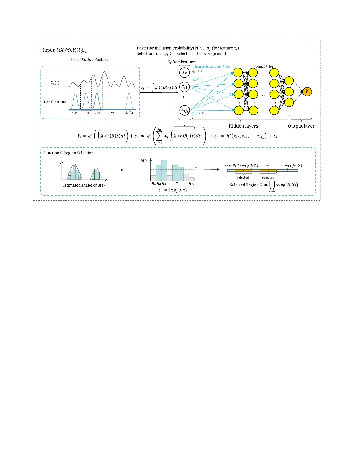
Sparse Bayesian Deep Functional Lear ning with Structur ed Region Selection Xiaoxian Zhu 1 Y ingmeng Li 1 Shuangge Ma 2 Mengyun W u 1 Abstract In modern applications such as ECG monitoring, neuroimaging, wearable sensing, and industrial equipment diagnostics, complex and continuously structured data are ubiquitous, presenting both challenges and opportunities for functional data analysis. Howe ver , e xisting methods face a criti- cal trade-off: con ventional functional models are limited by linearity , whereas deep learning ap- proaches lack interpretable region selection for sparse ef fects. T o bridge these gaps, we propose a sparse Bayesian functional deep neural network (sBayFDNN). It learns adaptiv e functional em- beddings through a deep Bayesian architecture to capture complex nonlinear relationships, while a structured prior enables interpretable, region- wise selection of inﬂuential domains with quanti- ﬁed uncertainty . Theoretically , we establish rigor- ous approximation error bounds, posterior consis- tency , and region selection consistency . These results provide the ﬁrst theoretical guarantees for a Bayesian deep functional model, ensuring its reliability and statistical rigor . Empirically , comprehensiv e simulations and real - world stud- ies conﬁrm the effecti veness and superiority of sBayFDNN. Crucially , sBayFDNN excels in rec- ognizing intricate dependencies for accurate pre- dictions and more precisely identiﬁes functionally meaningful regions, capabilities fundamentally beyond e xisting approaches. 1. Introduction W ith rapid technological advances, div erse ﬁelds—from healthcare to neuroscience—are generating increasingly complex data that e xhibit inherent structure and continuity ov er time or space. For instance, electrocardiogram (ECG) 1 School of Statistics and Data Science, Shanghai Univ ersity of Finance and Economics 2 Department of Biostatistics, Y ale School of Public Health. Correspondence to: Mengyun W u < wu.mengyun@mail.shufe.edu.cn > . Pr oceedings of the 43 rd International Conference on Machine Learning , Seoul, South K orea. PMLR 306, 2026. Copyright 2026 by the author(s). recordings are analyzed as functional curves to elucidate cardiac morphology and identify pathological patterns, of- fering insights into cardiov ascular health ( Pang et al. , 2023 ). Similarly , neuroimaging data are modeled as spatiotemporal ﬁelds to capture brain dynamics constrained by anatomical geometry , advancing the study of neural functions and dis- orders ( Tsai et al. , 2024 ). Such data are naturally vie wed as realizations of underlying functions and are suited for analysis within functional data analysis (FD A), which uses their smoothness and structure to model temporal or spatial patterns. The analysis of these functional observations is important, particularly in human health studies, where inter- preting such signals can inform diagnosis, monitoring, and treatment. In FDA, supervised learning with functional predictors is fundamentally important yet faces two major challenges. First, the relationship between functional predictors and responses is often intrinsically comple x and nonlinear . Ig- noring such nonlinearity risks signiﬁcant model misspeciﬁ- cation, potentially leading to poor predictiv e performance in real-world applications. Second, and more critically , many applications exhibit local sparsity or re gion-speciﬁc effects. This means the predictiv e relationship is not globally active across the entire function domain; instead, it is concentrated within one or a fe w speciﬁc, contiguous subregions (e.g., time intervals or wa velength bands) where the functional coefﬁcient is nonzero, while being negligible or zero else- where. Failure to account for this structure may introduce substantial noise and degrade both interpretability and esti- mation efﬁcienc y . These two challenges are commonly intertwined in practice. For example, in bedside monitoring, physiological wa ve- forms such as ECG—driv en by intricate and dynamic patho- physiological states—not only manifest highly comple x and nonlinear patterns but also frequently exhibit local sparsity ( Moor et al. , 2023 ). Speciﬁcally , clinically actionable in- formation is not distributed uniformly but is concentrated within physiologically meaningful regions of the wa veform, such as the QRS complex for arrhythmia analysis or the ST segment for ischemia detection. Signals from other inter- vals are often non-informative. This makes interpretable region selection a core enabling step, as it precisely tar gets the localized subdomains where complex nonlinear relation- ships are most acti ve and meaningful, thereby forming the 1 Sparse Bayesian Deep Functional Learning with Structur ed Region Selection foundation for efﬁcient and rob ust functional models. Supervised learning with functional data has been exten- siv ely studied. Classical functional linear regression (FLR) estimates smooth coefﬁcient functions but lacks inherent region selection—a limitation partially mitigated by later sparse FLR v ariants, though linearity constraints remain. Nonlinear functional models of fer ﬂexibility yet often de- pend on prespeciﬁed structures, limiting their capacity to capture highly complex relationships. While deep neural networks (DNNs) provide strong approximation po wer and hav e been adapted to functional settings, existing DNN- based methods focus predominantly on prediction and do not incorporate interpretable, structured region selection on the functional domain. Moreo ver , common DNN feature selection techniques are designed for scalar inputs and f ail to lev erage the continuous nature of functional data. These gaps underscore the need for a DNN framework that jointly handles nonlinear complexity and performs interpretable region selection in functional settings. W e propose a sparse Bayesian deep neural network (sBayFDNN) that integrates functional embedding learning with a Bayesian DNN architecture to perform interpretable region - wise selection for functional predictors. The model captures ﬂexible nonlinear function - to - scalar relationships while providing posterior inference for uncertainty quantiﬁ- cation. Our main contributions are: • A Bayesian Functional DNN Frame work with Uncer - tainty Quantiﬁcation: W e introduce a model that em- beds functional predictors through a deep Bayesian net- work to capture complex nonlinear associations with scalar responses. The framework deliv ers not only point estimates but als o posterior uncertainty , o vercom- ing the rigidity of traditional functional regression. • Interpretable Region Selection via Structured Sparsity: A sparse prior is imposed on the ﬁrst hidden layer to perform region-wise functional selection. This signiﬁ- cantly enhances model interpretability while mitigating the black - box nature of con ventional DNNs, yielding actionable insights into inﬂuential domains. • Theoretical Guarantees: W e establish rigorous theo- retical results, including approximation error bounds, posterior consistency , and region selection consistency . These provide the ﬁrst theoretical foundation for a Bayesian deep functional model, thereby opening a new v enue for statistically rigorous and interpretable functional deep learning. • Empirical V alidation: Comprehensiv e simulations and di verse real-world studies conﬁrm that sBayFDNN out- performs existing methods in both prediction accuracy and region identiﬁcation, especially in challenging sce- narios where con ventional models are misspeciﬁed or inﬂexible, demonstrating its practical superiority . 2. Related W orks 2.1. Classical functional regr ession methods Classical functional regression methods, represented by the functional linear model and its extensions, establish rela- tionships between functional predictors and scalar responses using techniques such as B-splines ( Cardot et al. , 2003 ), re- producing kernel Hilbert spaces ( Crambes et al. , 2009 ), and smoothing regularization ( Cai & Y uan , 2012 ). T o enhance interpretability , sparse penalization methods ha ve been intro- duced for local region selection, including sparse functional linear regression ( Lee & Park , 2012 ), smooth locally sparse estimators ( Lin et al. , 2017 ; Belli , 2022 ), and their Bayesian counterparts ( Zhu et al. , 2025 ). T o mov e beyond linearity , nonlinear methods such as functional single-inde x models hav e been proposed ( Jiang et al. , 2020 ), which can also achiev e local sparsity via penalization ( Nie et al. , 2023 ). Howe v er , these approaches f ace ke y limitations: linear mod- els cannot adequately capture complex nonlinear relation- ships, while existing nonlinear methods rely on pre-deﬁned kernels or bases, limiting their ﬂexibility and capacity to model intricate dependencies directly from data. 2.2. Deep Learning f or Functional Data Deep learning for functional data has advanced in recent years, with methods primarily aimed at enhancing repre- sentation learning and predicti ve performance. Early ap- proaches introduced adapti ve basis layers to learn data- driv en functional representations within DNNs ( Y ao et al. , 2021 ), and were followed by DNNs speciﬁcally designed for functional inputs ( Thind et al. , 2023 ) and classiﬁers b uilt on functional principal components ( W ang et al. , 2023 ). Autoencoder architectures hav e also been adapted for func- tional latent representation learning ( W u et al. , 2024 ). Despite their predictiv e power , these methods often operate as “black boxes”, lacking explicit mechanisms for region selection on the functional domain. This limits their utility in scientiﬁc applications where identifying which speciﬁc regions of the data dri ve predictions is essential. 2.3. Sparsity and Selection in Neural Networks A parallel line of research incorporates sparsity into neural networks for vector -valued inputs. This includes frame- works performing v ariable selection via group sparsity penalties on the ﬁrst hidden layer ( Dinh & Ho , 2020 ; Chu et al. , 2023 ; Luo & Halabi , 2025 ), architectures employing sparsity-inducing mechanisms on linear input layers ( Chen et al. , 2021 ; Atashgahi et al. , 2023 ), and residual layers used 2 Sparse Bayesian Deep Functional Learning with Structur ed Region Selection ) supp 𝐵 1 𝑡 supp 𝐵 𝐽 𝑛 𝑡 ⋯ ⋯ select ed select ed supp 𝐵 3 𝑡 τ ⋯ 𝐵 1 𝑡 𝐵 2 𝑡 𝐵 𝐽 𝑛 𝑡 𝐵 3 𝑡 𝑞 1 < 𝜏 𝑞 2 > 𝜏 𝑞 𝐽 𝑛 > 𝜏 Sparse Structur ed Prior Normal Prior F igur e 1. W orkﬂow of sBayFDNN. The functional predictor X i ( t ) is projected onto locally supported B-spline bases to form spline features x i = ( x i 1 , . . . , x i,J n ) ⊤ . A DNN with a spike-and-slab prior on the ﬁrst-layer weight columns yields feature-wise posterior inclusion probabilities (PIPs) q j , which are thresholded to select spline features and mapped back to the function domain to produce an estimated activ e region b Ω . to achiev e feature-wise sparsity ( Lemhadri et al. , 2021 ; Fan & W aldmann , 2025 ). Furthermore, Sun et al. ( 2022 ) pro- posed a Bayesian framew ork to learn sparse DNNs through connection pruning, establishing posterior consistency b ut not traditional input-le vel v ariable selection. Beyond vari- able selection, similar sparse DNN techniques hav e also been de veloped for applications in other ﬁelds, such as bi- ological or social network reconstruction ( F an et al. , 2025 ; Y ang et al. , 2026 ). While these techniques enhance interpretability for vector data, they are not designed to e xploit the continuous, struc- tured nature of functional inputs. Consequently , a signiﬁ- cant g ap remains for a method that integrates nonlinear deep learning with structured, interpretable region selection and uncertainty quantiﬁcation speciﬁcally for functional data. 3. Methodology Let X 1 ( t ) , . . . , X n ( t ) be n independent functional covari- ates deﬁned on the closed interv al T ⊂ R . For theoretical and computational purposes, T is standardized to [0 , 1] . Let Y i denote a scalar response. W e consider a functional single- index model (see Figure 1 for a schematic o vervie w): Y i = g ∗  Z T X i ( t ) β ( t ) dt  + ε i , (1) where ε i ∼ N (0 , σ 2 ε ) , β ( · ) is an unkno wn coefﬁcient func- tion, and g ∗ ( · ) is an unkno wn nonlinear function. Without loss of generality , we assume the domain of g ∗ ( · ) is [0 , 1] ; this can be achieved by suitably rescaling R T X i ( t ) β ( t ) dt and absorbing the scaling into the deﬁnition of g ∗ . For notational simplicity , we retain the original notation in the subsequent exposition. The function g ∗ ( · ) allo ws for a ﬂexible, potentially nonlinear relationship between the scalar response and the functional cov ariate through the single-index projection. Motiv ated by applications where the association is dri ven by only a fe w subregions of T (e.g., a small number of time intervals), we assume that β ( · ) is effecti v ely localized and aim to identify the corresponding activ e regions. T o circumvent the inﬁnite-dimensionality of β ( · ) , we ap- proximate it using a truncated B-spline basis expansion: β J n ( t ) = J n X j =1 w J n ,j B j ( t ) , (2) which yields the following ﬁnite-dimensional representa- tion: Y i ≈ g ∗  η ( X i ) ⊤ w J n  + ε i = h ∗  η ( X i )  + ε i . (3) 3 Sparse Bayesian Deep Functional Learning with Structur ed Region Selection by replacing β ( · ) with β J n ( · ) , where R T X i ( t ) β J n ( t ) dt = η ( X i ) ⊤ w J n . Here, { B j ( · ) } J n j =1 denotes a collec- tion of J n B-spline basis functions, and w J n := ( w J n , 1 , . . . , w J n ,J n ) ⊤ ∈ R J n is the corresponding v ec- tor of coef ﬁcients. The spline features η ( X i ) = ( x i 1 , . . . , x iJ n ) ⊤ ∈ R J n , where x ij := R T X i ( t ) B j ( t ) dt . W e further introduce h ∗ ( · ) , which absorbs the B-spline co- efﬁcient v ector w J n , thus reducing the problem to learning a ﬁnite-dimensional function. Next, we aim to estimate h ∗ ( · ) using a DNN F θ that takes η ( X i ) ∈ R J n as input. The network can be written as F θ = A H n ◦ σ ◦ A H n − 1 ◦ · · · ◦ σ ◦ A 1 . (4) Here, we consider a feedforward DNN with H n − 1 hidden layers and width L h at layer h , where L 0 = J n and L H n = 1 , with a common activ ation σ ( · ) in the hidden layers and a linear output layer . W e consider the ReLU activ ation in our study . Let θ = { ( W h , b h ) } H n h =1 , where W h ∈ R L h × L h − 1 and b h ∈ R L h denote the weights and biases. The af ﬁne map is deﬁned as A h ( u ) := W h u + b h . In ( 3 ), since the B-spline basis is locally supported, the localization of β ( · ) ov er T is naturally reﬂected in the sparsity pattern of w J n in ( 2 ) . Therefore, we consider the setting where w J n is sparse, so that η ( X i ) ⊤ w J n = η S J n ( X i ) ⊤ w S J n , where S J n ⊂ { 1 , . . . , J n } denotes an unknown support set, η S J n ( X i ) and w S J n denote the corre- sponding subv ectors. With ( 4 ), since w J n is absorbed into h ∗ ( · ) , the sparsity of w J n naturally translates into sparsity of the ﬁrst - layer weight matrix W 1 ∈ R L 1 × J n . Speciﬁcally , denoting by W 1 , ∗ j ∈ R L 1 the j -th column of W 1 , we hav e that if || W 1 , ∗ j || 2  = 0 , then j ∈ S J n . Based on ( 3 ) and ( 4 ), we propose a sparse Bayesian func- tional DNN (sBayFDNN) framework, employing the fol- lowing prior distrib utions for the model parameters: for j ∈ { 1 , . . . , J n } , W 1 , ∗ j | γ j ∼ h N (0 , σ 2 1 ,n I ) i γ j h N (0 , σ 2 0 ,n I ) i 1 − γ j , (5) π ( γ j ) ∼ Bern( λ n ) , (6) W h,ab ∼ N (0 , σ 2 ) , ∀ h ∈ { 2 , . . . , H n } , (7) b h,a ∼ N (0 , σ 2 ) , ∀ h ∈ { 1 , . . . , H n } . (8) Here, N ( c, d ) denotes the normal distribution with mean c and variance (cov ariance) d , and Bern( λ n ) denotes the Bernoulli distribution with success probability λ n ∈ (0 , 1) . The symbol I represents an identity matrix of appropriate dimensions. The entry W h,ab corresponds to the ( a, b ) - th element of the matrix W h , where a ∈ 1 , . . . , L h and b ∈ 1 , . . . , L h − 1 . Each γ j (for j ∈ 1 , . . . , J n ) is a binary indicator . W e set σ 2 1 ,n > σ 2 0 ,n > 0 , with σ 2 0 ,n taken to be a small positiv e v alue, and let σ 2 > 0 . As introduced abo ve, distinct priors are speciﬁed for the ﬁrst layer and the subsequent layers. T o enable functional region selection in the spline - feature domain, we impose a group - wise continuous spike - and - slab prior on each W 1 , ∗ j for j = 1 , . . . , J n . When γ j = 0 , the spike variance σ 2 0 ,n strongly shrinks all entries of W 1 , ∗ j tow ard zero with high probability; when γ j = 1 , the slab v ariance σ 2 1 ,n permits the entries to take appreciable nonzero values, thereby allo wing the corresponding spline - basis feature to contribute to the functional representation. For the remaining layers, weights and biases are assigned entrywise independent Gaussian priors N (0 , σ 2 ) , which preserves the ﬂexibility needed in the hidden layers to learn complex, nonlinear patterns based on the features identiﬁed by the ﬁrst hidden layer . 4. Optimization-based Bayesian Infer ence The proposed Bayesian inference proceeds via three steps: (i) compute a (local) posterior mode (MAP) of the network parameters under the mar ginal prior; (ii) deriv e feature-le v el posterior inclusion probabilities from the ﬁrst - layer; and (iii) map the selected spline features to an estimated acti ve region. The detailed procedure is described below , and the hyperparameter settings are provided in the Appendix. 4.1. MAP ﬁtting For θ , we optimize the marginal posterior in which the inclusion indicators γ are integrated out, and denote the resulting mar ginal prior by π ( θ ) . Then, we compute a MAP by minimizing the negati ve log-posterior objecti v e ˆ θ ∈ arg min θ 1 2 σ 2 ε n X i =1  Y i − f θ ( η ( X i ))  2 − log π ( θ ) , (9) where f θ is the H n -layer feedforward network deﬁned in ( 4 ). Optimization is carried out using stochastic gradient methods (see Appendix for the detailed algorithm). 4.2. MAP plug-in posterior inclusion probabilities Denote A 1 ,n = λ n ( σ 2 1 ,n ) − L 1 / 2 and A 0 ,n = (1 − λ n )( σ 2 0 ,n ) − L 1 / 2 . Then, for each feature index j , apply- ing Bayes’ rule to (5) and (6) gives the conditional poste- rior inclusion probability (PIP): Pr( γ j = 1 | W 1 , ∗ j ) = A 1 ,n exp  − ∥ W 1 , ∗ j ∥ 2 2 2 σ 2 1 ,n  A 1 ,n exp  − ∥ W 1 , ∗ j ∥ 2 2 2 σ 2 1 ,n  + A 0 ,n exp  − ∥ W 1 , ∗ j ∥ 2 2 2 σ 2 0 ,n  . W e compute plug - in PIP ˆ q j := Pr( γ j = 1 | ˆ W 1 , ∗ j ) based on the MAP estimate ˆ θ and select spline features by thresh- olding: b S τ := { j : ˆ q j > τ } with default τ = 1 / 2 . Since ˆ q j is monotone in ∥ ˆ W 1 , ∗ j ∥ 2 2 , this rule is equi valent to thresh- olding the ﬁrst-layer column norms. 4 Sparse Bayesian Deep Functional Learning with Structur ed Region Selection 4.3. Mapping selected features to an acti ve region on T Giv en b S τ ⊂ { 1 , . . . , J n } , we map the selected spline fea- tures back to the functional domain using the local support of B-splines. Let supp( B j ( t )) ⊂ T denote the support of the j th basis function. W e deﬁne the estimated acti ve re gion as b Ω := S j ∈ b S τ supp( B j ) , and represent b Ω as a union of disjoint subintervals by mer ging adjacent components. 5. Theoretical Pr operties Let β ∗ and β ∗ J n be the true coefﬁcient function and its trun- cated counterpart, respecti vely . Let ω ∗ J n ∈ R J n be the vec- tor of true basis coefﬁcients for β ∗ J n , S ∗ J n = supp( ω ∗ J n ) its support, and s n = | S ∗ J n | the sparsity lev el. Deﬁne e ∗ j = I ( j ∈ S ∗ J n ) as the true binary selection indicator and Ω ∗ ⊂ T as the true non-zero region of β ∗ . Denote Ω ∗ ( κ ) = { t ∈ T : | β ∗ ( t ) | > κ } as the strong-signal re- gion and Ω ∗ ( κ ) c as its complement. Denote a n ≲ b n if a n ≤ C b n for some constant C > 0 , and a n ≍ b n if c b n ≤ a n ≤ C b n for constants 0 < c < C . Denote µ ∗ ( X ) = g ∗  R T X ( t ) β ∗ ( t ) dt  as the true mean function and µ θ ( X ) := F θ ( η ( X )) as the network out- put deﬁned in ( 4 ). Consider the class of fully-connected, J n -input ReLU networks, denoted by N N J n ( H n , ¯ L, E n ) , with depth H n , constant maximum hidden width ¯ L = max 2 ≤ k ≤ H n L k , and parameter bound ∥ θ ∥ ∞ ≤ E n . W e deﬁne the column-wise support of the network parameters as supp col ( θ ) = { j ∈ { 1 , · · · , J n } : ∥ W 1 , ∗ j ∥ 2 > 0 } . For any subset T ⊂ { 1 , · · · , J n } , the associated column-sparse network class is deﬁned as N N col J n ( T ; H n , ¯ L, E n ) :=  F θ ∈ N N J n ( H n , ¯ L, E n ) : supp col ( θ ) = T  . The following assumptions are imposed. Assumption 5.1. sup X i ∈X R T | X i ( t ) | dt ≤ C X , where X de- notes the function space to which X i ( t ) belongs, and C X is a positiv e constant . Assumption 5.2. β ∗ ( t ) ∈ H α β ([0 , 1]) for some α β > 0 , where H α ( I ) denotes the H ¨ older space of functions on an interval I with smoothness order α . Ω ∗ is a ﬁnite union of intervals and   Ω ∗ ( κ J n ) c   → 0 , as n → ∞ , with κ J n = c κ C β J − α β n , where c κ > 4 and C β are constants deﬁned in Lemma B.1 (Appendix). Moreover , the strong-signal region has proportional size in the sense that | Ω ∗ ( κ J n ) | | Ω ∗ | ≥ c Ω for some constant c Ω ∈ (0 , 1] and all suf ﬁciently large n . Assumption 5.3. g ∗ ( · ) ∈ H α g ([0 , 1]) for some constant α g > 0 . These are standard regularity conditions in functional data analysis ( Cai & Y uan , 2012 ; Nie et al. , 2023 ). Assumption 5.1 ensures the well-posedness of the problem by uniformly bounding the predictor trajectories. Assumption 5.2 imposes H ¨ older smoothness on β ∗ , guaranteeing its accurate spline approximation. W e further assume the active region Ω ∗ is not overly complex, which excludes highly fragmented supports and aligns with typical domain-selection interpre- tations. Crucially , we require that the strong-signal re gion essentially cov ers Ω ∗ up to a negligible set; this acts as a minimum-signal condition in the functional setting, en- suring that the nonzero part of β ∗ is detectable enough to translate basis selection into faithful support recovery on the domain. W e further focus on the practically common proportional sparsity regime, where the strong-signal region retains a non-v anishing fraction of the activ e domain, which, under locally supported spline bases, implies that the num- ber of active groups scales as s n ≍ J n . Assumption 5.3 similarly enforces smoothness on the nonparametric link function, thereby supporting stable estimation. Theorem 5.4. Suppose that Assumptions 5.1 – 5.3 hold. Then: (i) Ther e exists a network par ameter vector θ such that: F θ = F ∈ N N col J n ( S ∗ J n ; H n , ¯ L, E n ) , (ii) W ith α 1 = min( α g , 1) , sup X ∈X | µ θ ( X ) − µ ∗ ( X ) | ≲ H − 2 α 1 n + J − α β α 1 n . Theorem 5.4 establishes that the true sparse model structure is exactly representable within the proposed architecture (i) and provides a non-asymptotic error bound (ii). This bound guarantees that the approximation error decays to zero as the network depth H n and the number of spline bases J n grow , with the rates gov erned by the smoothness of both the functional coefﬁcient β ( t ) and the link function g ∗ ( · ) . Assumption 5.5. For some constants τ ′ > 0 and α σ > 0 : λ n ≲ 1 J n  ( n ¯ L ) H n ( J n +1) L 1  τ ′ , E 2 n H n (log n +log ¯ L ) ≲ σ 2 1 ,n ≲ n α σ , and E 2 n H n (log n +log ¯ L ) ≲ σ 2 . Assumption 5.6. The DNN F θ in ( 4 ) satisﬁes: ¯ L ≍ L 1 ≍ 1 , H n ≍ min  J α β / 2 n , s n  with s n ≍ J n , and ∥ θ ∥ ∞ ≤ E n , where E n = n c 1 for some positiv e constant c 1 . Assumption 5.5 speciﬁes the rates for key hyperparameters in the Bayesian frame work, ensuring the prior is suf ﬁciently diffuse to permit effecti ve posterior contraction toward the true parameter , a standard requirement in Bayesian theory ( Ghosal et al. , 2000 ). Assumption 5.6 links the netw ork depth H n to the sparsity lev el s n so that architectural growth respects the intrinsic sparse structure. Similar conditions are commonly adopted in related theoretical analyses. Let Π( A | D n ) denote the posterior probability of an ev ent A giv en the observ ed data D n = { ( X i , Y i ) } n i =1 . Let p µ ∗ ( · | X ) be the true conditional density of Y giv en X , 5 Sparse Bayesian Deep Functional Learning with Structur ed Region Selection p µ θ ( · | X ) be the approximate density induced by the ﬁnite- dimensional representation ( 3 ) and the sparse DNN deﬁned in ( 4 ), and d ( · , · ) denote the Hellinger distance. Theorem 5.7. Suppose that Assumptions 5.1 – 5.6 hold and there exists an err or sequence ε 2 n satisfying ε 2 n ≲ s n log( J n /s n ) n + s n  H n log n +log J n  n +  H − 2 α 1 n + J − α β α 1 n  2 such that σ 2 0 ,n ≤ ˜ M n, 1 ( ε n ) and max { σ 2 , σ 2 0 ,n , σ 2 1 ,n } ≤ ˜ M n, 2 ( ε n ) , wher e ˜ M n, 1 ( ε n ) and ˜ M n, 2 ( ε n ) ar e deﬁned in ( 18 ) and ( 19 ) of Appendix. Then, for some constant c > 0 , we have P h Π  d ( p µ θ , p µ ∗ ) > 4 ε n | D n  ≥ 2 exp( − c n ε 2 n ) i ≤ 2 exp( − c n ε 2 n ) , and E h Π  d ( p µ θ , p µ ∗ ) > 4 ε n | D n  i ≤ 4 exp( − 2 c n ε 2 n ) . Theorem 5.7 establishes the posterior contraction rate ε n of sBayFDNN. This result implies that, with high probabil- ity , the posterior distribution concentrates around the true data - generating process at rate ε n . Speciﬁcally , if α β ≤ 2 , then H n ≍ J α β / 2 n , setting J n ≍  n log n  1 1+ α β / 2+2 α β α 1 yields ε 2 n ≍  log n n  2 α β α 1 1+ α β / 2+2 α β α 1 . If α β > 2 , then H n ≍ s n , taking J n ≍  n log n  1 2+4 α 1 leads to ε 2 n ≍  log n n  2 α 1 1+2 α 1 . Further , deﬁne the structural dif ference as ρ n ( ε n ) := max 1 ≤ j ≤ J n E h | γ j − e ∗ j | · I { θ / ∈ A n ( ε n ) }    D n i , where E ( ·| D n ) is the conditional expect ation, and A n ( ε n ) = n θ : d  p µ θ , p µ ∗  ≥ ε n o . Assumption 5.8. ρ n (4 ε n ) → 0 as n → ∞ and ε n → 0 . Assumption 5.8 serv es as an identiﬁability condition. It implies that as n → ∞ and ε n → 0 , any candidate model that is close to the true data-generating process in terms of Hellinger distance must asymptotically share the same underlying structure, thereby guaranteeing the consistent selection ( Sun et al. , 2022 ). Theorem 5.9. Suppose Assumptions 5.1 – 5.8 hold. Then: (i) max 1 ≤ j ≤ J n   ˆ q j − e ∗ j   P − → 0 . (ii) P  S ∗ J n ⊂ b S τ  → 1 for any pr especiﬁed τ ∈ (0 , 1) . (iii) P  b S 1 / 2 = S ∗ J n  → 1 . (iv) | b Ω∆Ω ∗ | P − → 0 . Theorem 5.9 establishes the asymptotic consistency of spline feature selection based on MAP plug-in posterior probabilities, showing that the estimated selection probabil- ities con ver ge to the true binary indicators. Furthermore, it guarantees the asymptotically exact reco very of the nonzero region in the continuous function domain from its discrete coefﬁcient support, thereby achie ving exact structural selec- tion for the functional effect. 6. Experiments W e e valuate sBayFDNN on synthetic and real-world func- tional data against ﬁv e competitors: (1) FNN, a spline- feature-based feedforward network using truncated basis expansion ( Thind et al. , 2023 ); (2) AdaFNN, which learns adaptiv e basis functions via auxiliary networks ( Y ao et al. , 2021 ); (3) cFuSIM, a functional single-inde x method with localized regularization ( Nie et al. , 2023 ); (4) BFRS, a Bayesian functional region selector with neighborhood structure ( Zhu et al. , 2025 ); and (5) SLoS, a functional lin- ear estimator with local sparsity via an fSCAD penalty ( Lin et al. , 2017 ). Predictive RMSE is reported for all methods; region-reco very metrics (Recall, Precision, F1) are provided only for sBayFDNN, cFuSIM, BFRS, and SLoS, as FNN and AdaFNN do not perform region selection. 6.1. Simulation Studies Our simulation studies v ary three ke y aspects: (1) the true coefﬁcient function β ∗ ( t ) , which spans a single interior bump (Simple), a boundary bump (Medium), and a pair of narrow oscillating peaks (Comple x); (2) the link function g ∗ , taken as linear , logistic, sinusoidal, or a composite nonlinear form; and (3) the response signal - to - noise ratio (SNR), set to 5 or 10. Functional covariates are generated from a truncated cosine basis, observed on a discrete grid with added measurement noise (see Appendix for full details). Figure 2 summarizes region-recov ery performance (F1 score) across all simulation scenarios (see Appendix for Recall and Precision). sBayFDNN consistently achieves high mean F1 with tight interquartile ranges, demonstrating robust and stable region identiﬁcation across both linear and nonlinear regimes. Its advantage is more pronounced in more challenging scenarios with lower signal-to-noise ratios, as well as under harder localization regimes and complex nonlinear link functions g ∗ . By contrast, sev eral baselines exhibit increased dispersion and more frequent low-F1 outcomes as mo ves aw ay from central support or g ∗ departs from linearity . The distributions also suggest dif ferent selection behaviors across methods. For example, cFuSIM often returns broader acti ve re gions (capturing truly acti ve interv als but at the cost of more false positiv es), whereas linear region-selection 6 Sparse Bayesian Deep Functional Learning with Structur ed Region Selection Linear Logic Sin Composite Low SNR High SNR Low SNR High SNR Low SNR High SNR Low SNR High SNR Simple Medium Complex sBayFDNN cFuSIM BFRS SLoS sBayFDNN cFuSIM BFRS SLoS sBayFDNN cFuSIM BFRS SLoS sBayFDNN cFuSIM BFRS SLoS sBayFDNN cFuSIM BFRS SLoS sBayFDNN cFuSIM BFRS SLoS sBayFDNN cFuSIM BFRS SLoS sBayFDNN cFuSIM BFRS SLoS 0.2 0.4 0.6 0.8 1.0 0.2 0.4 0.6 0.8 1.0 0.2 0.4 0.6 0.8 1.0 F1 score sBayFDNN cFuSIM BFRS SLoS F igur e 2. F1 scores across g functions, SNR settings, and β ( t ) scenarios. baselines deteriorate under strong nonlinearity due to model misspeciﬁcation. In contrast, sBayFDNN maintains a better balance between recall and precision. Beyond aggregate metrics, we further ev aluate uncertainty quantiﬁcation. T ak- ing the high-SNR, Medium- β , logistic-link scenario as an example, Figure 3 presents the posterior selection proba- bilities from sBayFDNN. These probabilities closely align with the true coef ﬁcient function, demonstrating the model’ s capacity to effecti v ely capture selection uncertainty . 0.0 0.2 0.4 0.6 0.8 1.0 t 0.0 0.5 1.0 PIP/Magnitude A verage PIP shape of β ( t ) F igur e 3. PIPs from sBayFDNN in the high-SNR, Medium- β , logistic-link scenario. Figure 4 shows that sBayFDNN achie v es the lowest or near - lowest mean RMSE in most scenarios, with concentrated distributions, indicating that region interpretability does not come at the cost of predictive performance. Its advantage is most evident under nonlinear links, where ﬂe xible function approximation is crucial. Here, sBayFDNN substantially outperforms the spline-based FNN, matches the accuracy of AdaFNN with greater stability , and surpasses cFuSIM when nonlinearity is pronounced. Linear methods (BFRS, SLoS) remain competiti ve only under nearly linear settings, with performance degrading sharply as nonlinearity increases. T ogether , these results afﬁrm the sBayFDNN framew ork: structured sparsity in the ﬁrst layer supports interpretable region identiﬁcation with inherent uncertainty quantiﬁcation, while subsequent deep layers furnish the ﬂexibility needed for accurate nonlinear prediction. 6.2. Real data analysis W e e valuate our method on four benchmark datasets: ECG, T ecator, Bike rental, and IHPC, using their ofﬁcial train/validation/test splits throughout. In the ECG task, Lead - II signals are used as functional inputs to predict the QRS duration—a clinically informativ e measure of ventric- ular depolarization relev ant for detecting conduction abnor - malities ( Hummel et al. , 2009 ; Kashani & Barold , 2005 ). For the T ecator dataset, near - infrared absorbance spectra of meat samples serve as functional inputs to predict w ater content ( Thodberg , 2015 ). In the Bike rental forecasting task ( Fanaee-T , 2013 ), the daily rental - demand proﬁle (a 24 - point curve) is used to predict total rentals ov er the fol- lowing 7 days. For the IHPC dataset ( Hebrail & Berard , 2006 ), daily minute - av eraged activ e - power trajectories are taken as functional inputs to predict the next - day total energy usage. W e report standard predictiv e metrics (RMSE/MAE) for all datasets. For ECG and T ecator , silver - standard re- gion annotations are av ailable, allo wing us to also ev aluate region - identiﬁcation metrics. Detailed data information are provided in the Appendix. As shown in T able 1 and 2 , sBayFDNN delivers the strongest ov erall performance across all datasets. While all methods attain relati vely lo w precision in re gion selection, sBayFDNN achie ves substantially higher recall and F1. Fig- ure 5 plots the estimated PIPs on the original domains with sBayFDNN for ECG and T ecator . For ECG, sBayFDNN as- signs higher inclusion strength within and near the clinically moti vated QRS interv al (shaded), with PIP values approach- ing 1 close to the boundaries, consistent with the fact that duration is determined by onset/of fset timing and thus end- point morphology is most informativ e. For T ecator , the PIP increases within the predeﬁned water band (965–985 nm; shaded), while additional elev ated PIP regions appear at earlier wa velengths (including ∼ 930 nm, often regarded as lipid/fat-associated in short-wa ve NIR), plausibly reﬂecting 7 Sparse Bayesian Deep Functional Learning with Structur ed Region Selection Linear Logic Sin Composite Low SNR High SNR Low SNR High SNR Low SNR High SNR Low SNR High SNR 1.0 2.0 3.0 0.5 1.0 1.5 0.2 0.4 0.6 0.4 0.6 0.2 0.4 0.6 0.5 5.0 10 10 15 0.5 1.0 1.5 0.5 1.0 0.2 0.4 0.6 0.8 0.4 0.6 0.8 0.2 0.4 0.5 1.0 5.0 6.0 7.0 7.0 8.0 9.0 10 sBayFDNN FNN AdaFNN cFuSIM BFRS SLoS sBayFDNN FNN AdaFNN cFuSIM BFRS SLoS sBayFDNN FNN AdaFNN cFuSIM BFRS SLoS sBayFDNN FNN AdaFNN cFuSIM BFRS SLoS sBayFDNN FNN AdaFNN cFuSIM BFRS SLoS sBayFDNN FNN AdaFNN cFuSIM BFRS SLoS sBayFDNN FNN AdaFNN cFuSIM BFRS SLoS sBayFDNN FNN AdaFNN cFuSIM BFRS SLoS 0.6 0.8 1.0 1.2 1.0 1.5 0.2 0.4 0.6 0.3 0.4 0.5 0.6 0.1 0.2 0.3 0.2 0.3 0.4 1.5 2.0 2.0 2.5 3.0 S i m p l e M e d i u m C o m p l e x sBayFDNN FNN AdaFNN cFuSIM BFRS SLoS R M S E F igur e 4. RMSE across g functions, SNR settings, and β ( t ) scenarios. T able 1. Performance on ECG and T ecator datasets. F1, Recall, and Precision are reported only for methods that output an estimated activ e region; otherwise sho wn as “–”. Best results within each dataset/metric are in bold. ECG T ecator Method RMSE MAE F1 Recall Precision RMSE MAE F1 Recall Precision sBayFDNN 12.069 8.711 0.634 1.000 0.464 2.138 1.594 0.339 1.000 0.204 FNN 12.991 9.239 – – – 2.217 1.613 – – – AdaFNN 14.083 10.198 – – – 3.027 2.299 – – – cFuSIM 17.677 12.861 0.501 1.000 0.334 3.932 3.283 0.137 0.977 0.074 BFRS 16.297 11.805 0.396 0.784 0.265 2.691 2.250 0.211 0.714 0.124 SLoS 16.258 11.782 0.412 0.815 0.276 2.567 2.068 0.228 0.854 0.132 T able 2. Performance on Bike rental and IHPC datasets. Bike IHPC Method RMSE MAE RMSE MAE sBayFDNN 0.618 0.497 0.536 0.409 FNN 0.699 0.535 0.549 0.409 AdaFNN 0.720 0.577 0.552 0.420 cFuSIM 0.693 0.539 0.548 0.411 BFRS 0.749 0.550 0.552 0.416 SLoS 0.684 0.506 0.549 0.411 strong collinearity/compositional coupling between water and fat and other broad predicti ve structure. These results demonstrate that sBayFDNN can reco ver physically inter- pretable regions without sacriﬁcing predicti ve accurac y . 7. Conclusion W e hav e presented a sparse Bayesian functional DNN frame- work that performs automatic region selection for nonlinear scalar - on - function regression. By integrating B - spline ex- pansions with a Bayesian neural network and imposing a structured spik e - and - slab prior , our model captures complex nonlinear dependencies between functional predictors and scalar responses through data - driv en functional represen- tations and a ﬂexible deep architecture. The frame work provides interpretable re gion-wise selection and principled uncertainty quantiﬁcation, supported by theoretical guaran- tees. Simulations and experiments on multiple real - world datasets conﬁrm its selection accuracy and competitiv e pre- dictiv e performance, demonstrating practical utility in iden- tifying region-speciﬁc functional ef fects. −300 −200 −100 0 100 200 300 Time r elative to R-peak (ms) 0.00 0.25 0.50 0.75 1.00 A verage PIP ECG 850 900 950 1000 1050 W avelength (nm) T ecator A verage PIP Silver interval F igur e 5. PIPs from sBayFDNN for ECG and T ecator datasets. Future work includes extending the framew ork to jointly model functional and discrete cov ariates, rather than pre - adjusting for confounders. The approach can also be generalized to handle multiple functional predictors with simultaneous v ariable and region selection. Replacing the l 2 loss with a more robust alternativ e may improve stabil- ity in noisy settings, while embedding the model within a generalized linear model would allo w applications to binary , count, or surviv al outcomes, further broadening its utility in functional data analysis. 8 Sparse Bayesian Deep Functional Learning with Structur ed Region Selection Software and Data The implementation code for sBayFDNN is available in the Supplementary Material, while the do wnload link for the accompanying real dataset is pro vided in the Appendix. Impact Statement This work introduces a Bayesian deep learning frame work for interpretable region selection in functional data. It ad- vances nonlinear function - to - scalar regression by integrat- ing structured sparsity with principled uncertainty quantiﬁ- cation. The primary aim is to enhance machine learning methodology for functional and structured data. The pro- posed framework beneﬁts domains where interpretability and reliability are essential, such as spectral chemometrics, neural signal analysis, and clinical monitoring. By enabling precise identiﬁcation of informativ e functional subdomains, the method can support more accurate material composi- tion analysis, reﬁned physiological signal interpretation, and more targeted diagnostic interv entions. References Atashgahi, Z., Zhang, X., Kichler , N., Liu, S., Y in, L., Pechenizkiy , M., V eldhuis, R., and Mocanu, D. C. Super- vised feature selection with neuron e volution in sparse neural networks. T ransactions on Machine Learning Resear ch , 2023. ISSN 2835-8856. URL https:// openreview.net/forum?id=GcO6ugrLKp . Fea- tured Certiﬁcation. Belli, E. Smoothly adaptiv ely centered ridge estimator . Journal of Multivariate Analysis , 189:104882, 2022. Cai, T . T . and Y uan, M. Minimax and adaptive prediction for functional linear regression. J ournal of the American Statistical Association , 107(499):1201–1216, 2012. Cardot, H., Ferraty , F ., and Sarda, P . Spline estimators for the functional linear model. Statistica Sinica , pp. 571– 591, 2003. Chen, Y ., Gao, Q., Liang, F ., and W ang, X. Nonlinear variable selection via deep neural networks. Journal of Computational and Graphical Statistics , 30(2):484–492, 2021. Chu, Z., Claridy , M., Cordero, J., Li, S., and Rathbun, S. L. Estimating propensity scores with deep adaptive v ariable selection. In Pr oceedings of the 2023 SIAM International Confer ence on Data Mining (SDM) , pp. 730–738. SIAM, 2023. Crambes, C., Kneip, A., and Sarda, P . Smoothing splines estimators for functional linear regression. The Annals of Statistics , 37(1):35–72, 2009. Dinh, V . C. and Ho, L. S. Consistent feature selection for analytic deep neural networks. Advances in Neural Information Pr ocessing Systems , 33:2420–2431, 2020. 9 Sparse Bayesian Deep Functional Learning with Structur ed Region Selection Elias, P . and Finer, J. EchoNext: A Dataset for Detect- ing Echocardiogram-Conﬁrmed Structural Heart Dis- ease from ECGs. PhysioNet , September 2025. doi: 10.13026/3ykd- bf14. URL https://doi.org/10. 13026/3ykd- bf14 . V ersion 1.1.0. Fan, J., Y ang, J., Ma, S., and W u, M. Bilev el network learning via hierarchically structured sparsity . In The Thirty-ninth Annual Confer ence on Neural Information Pr ocessing Systems , 2025. Fan, Y . and W aldmann, P . Multi-task genomic prediction using gated residual variable selection neural networks. BMC Bioinformatics , 26(1):167, 2025. Fanaee-T , H. Bike Sharing. UCI Machine Learning Reposi- tory , 2013. DOI: https://doi.org/10.24432/C5W894. Ghosal, S., Ghosh, J. K., and V an Der V aart, A. W . Con- ver gence rates of posterior distributions. The Annals of Statistics , 28(2):500–531, 2000. Goldberger , A. L., Amaral, L. A., Glass, L., Hausdorff, J. M., Ivano v , P . C., Mark, R. G., Mietus, J. E., Moody , G. B., Peng, C.-K., and Stanley , H. E. Physiobank, physiotoolkit, and physionet: components of a new research resource for complex physiologic signals. Cir culation , 101(23): e215–e220, 2000. Hebrail, G. and Berard, A. Individual Household Electric Power Consumption. UCI Machine Learning Repository , 2006. DOI: https://doi.org/10.24432/C58K54. Hummel, S. L., Skorcz, S., and K oelling, T . M. Prolonged electrocardiogram qrs duration independently predicts long-term mortality in patients hospitalized for heart fail- ure with preserved systolic function. J ournal of Car diac F ailur e , 15(7):553–560, 2009. Jiang, F ., Baek, S., Cao, J., and Ma, Y . A functional single- index model. Statistica sinica , 30(1):303–324, 2020. Jiang, W . Bayesian variable selection for high dimensional generalized linear models: Conv ergence rates of the ﬁtted densities. The Annals of Statistics , 35(4):1487–1511, 2007. Kachuee, M., F azeli, S., and Sarrafzadeh, M. Ecg heart- beat classiﬁcation: A deep transferable representation. In 2018 IEEE International Conference on Healthcar e Informatics (ICHI) , pp. 443–444. IEEE, 2018. Kashani, A. and Barold, S. S. Signiﬁcance of qrs com- plex duration in patients with heart failure. Journal of the American Colle ge of Car diology , 46(12):2183–2192, 2005. Lee, E. R. and P ark, B. U. Sparse estimation in functional linear regression. J ournal of Multivariate Analysis , 105 (1):1–17, 2012. Lemhadri, I., Ruan, F ., Abraham, L., and Tibshirani, R. Lassonet: A neural network with feature sparsity . Journal of Machine Learning Resear c h , 22(127):1–29, 2021. Lin, Z., Cao, J., W ang, L., and W ang, H. Locally sparse estimator for functional linear regression models. J ournal of Computational and Graphical Statistics , 26(2):306– 318, 2017. Luo, B. and Halabi, S. Sparse-input neural network using group concav e regularization. T ransactions on Machine Learning Researc h , 2025. ISSN 2835- 8856. URL https://openreview.net/forum? id=m9UsLHZYeX . Featured Certiﬁcation. Mako wski, D., Pham, T ., Lau, Z. J., Brammer , J. C., Lespinasse, F ., Pham, H., Sch ¨ olzel, C., and Chen, S. A. Neurokit2: A python toolbox for neurophysiological sig- nal processing. Behavior Researc h Methods , 53(4):1689– 1696, 2021. Moor , M., Banerjee, O., Abad, Z. S. H., Krumholz, H. M., Leskov ec, J., T opol, E. J., and Rajpurkar , P . Founda- tion models for generalist medical artiﬁcial intelligence. Natur e , 616(7956):259–265, 2023. Nie, Y ., W ang, L., and Cao, J. Estimating functional single index models with compact support. Envir onmetrics , 34 (2):e2784, 2023. Pang, J. C., Aquino, K. M., Oldehinkel, M., Robinson, P . A., Fulcher , B. D., Breakspear , M., and Fornito, A. Geometric constraints on human brain function. Natur e , 618(7965):566–574, 2023. Sun, Y ., Song, Q., and Liang, F . Consistent sparse deep learning: Theory and computation. Journal of the Ameri- can Statistical Association , 117(540):1981–1995, 2022. Thind, B., Multani, K., and Cao, J. Deep learning with func- tional inputs. Journal of Computational and Gr aphical Statistics , 32(1):171–180, 2023. Thodberg, H. H. T ecator meat sample dataset. StatLib Datasets Archiv e, 2015. http://lib.stat.cmu. edu/datasets/tecator . Tsai, K., Zhao, B., K oyejo, S., and Kolar , M. Latent mul- timodal functional graphical model estimation. J ournal of the American Statistical Association , 119(547):2217– 2229, 2024. van Kollenb urg, G. H., van Manen, H.-J., Admiraal, N., Gerretzen, J., and Jansen, J. J. Lo w-cost handheld nir 10 Sparse Bayesian Deep Functional Learning with Structur ed Region Selection spectroscopy for identiﬁcation of organic solvents and low-le v el quantiﬁcation of water contamination. T alanta , 223:121865, 2021. W ang, S., Cao, G., Shang, Z., and Initiative, A. D. N. Deep neural network classiﬁer for multidimensional functional data. Scandinavian Journal of Statistics , 50(4):1667– 1686, 2023. W u, S., Beaulac, C., and Cao, J. Functional autoencoder for smoothing and representation learning. Statistics and Computing , 34(6):203, 2024. Y ang, J., Li, T ., W ang, T ., Ma, S., and W u, M. Heteroge- neous gene network estimation for single-cell transcrip- tomic data via a joint regularized deep neural network. Journal of the American Statistical Association , (just- accepted):1–16, 2026. Y ao, J., Mueller , J., and W ang, J.-L. Deep learning for functional data analysis with adaptiv e basis layers. In In- ternational Confer ence on Machine Learning , pp. 11898– 11908. PMLR, 2021. Y arotsky , D. Optimal approximation of continuous func- tions by very deep relu networks. In Confer ence on Learn- ing Theory , pp. 639–649. PMLR, 2018. Y u, C., Lin, H., Zhang, Q., and Sanderson, J. High prev a- lence of left ventricular systolic and diastolic asynchrony in patients with congestive heart failure and normal qrs duration. Heart , 89(1):54–60, 2003. Zhu, H., Sun, Y ., and Lee, J. Bayesian functional region selection. Stat , 14(1):e70047, 2025. Zubkov , A. M. and Serov , A. A. A complete proof of univ ersal inequalities for the distribution function of the binomial law . Theory of Pr obability & Its Applications , 57(3):539–544, 2013. 11 Sparse Bayesian Deep Functional Learning with Structur ed Region Selection A. Details f or the posterior inference A.1. Hyperparameter settings All responses Y are standardized using training-set statistics; unless otherwise stated, all computations are carried out on this standardized scale and we set the noise variance to σ 2 ε = 1 . For non-sparsiﬁed network parameters, we use independent Gaussian priors with v ariance σ 2 = 1 (numerically equal to σ 2 ε under standardization, b ut conceptually distinct). W e use R = 5 random restarts for each J n . Simulation defaults. • Basis: B-splines with degree 4 (unless otherwise stated). • Network: fully-connected ReLU, 64 – 64 – 64 – 1 ; ﬁrst-layer column-wise spike-and-slab selection. • Optimizer: mini-batch SGD, learning rate 10 − 3 , batch size 64, max 80,001 iterations, early stopping patience 3,000. • Spike-and-slab: ( λ n , σ 2 0 ,n , σ 2 1 ,n ) = (10 − 5 , 10 − 5 , 2 × 10 − 3 ) . W e treat the projection truncation level J n as a resolution hyperparameter and select it via restart-aggregated evidence in simulations or restart-aggregated validation loss when evidence computation is prohibiti ve. W e use the candidate set J = { 55 , 60 , 70 , 80 } for J n in simulations; for real datasets, J is chosen as a small neighborhood around a dataset-speciﬁc baseline resolution. W e train with a small learning rate and a relatively large early-stopping patience to obtain stable solutions across restarts. The sparsiﬁcation prior is intentionally strong in simulations; empirically , the same default sparsiﬁcation hyperparameters remain effecti v e on ECG ( n ≈ 2 – 3 × 10 4 ), consistent with increasingly data-dominated inference as n gro ws. For competing methods, we aim to ensure fair comparisons by using comparable model capacity whenev er applicable (e.g., similar depth/width for neural-network baselines). Method-speciﬁc hyperparameters are taken from authors’ recommended defaults when a vailable, and otherwise selected by cross-v alidation or v alidation loss on the same training/validation split. A.2. Stochastic gradient algorithm (SGD) for the MAP ﬁtting W e ﬁrst provide the deriv ations on the marginal prior on θ . Denote K 1 n = ( J n + 1) L 1 + P H n k =2 ( L k − 1 + 1) L k as the dimension of θ and W ⊂ { 1 , . . . , K 1 n } as the set of indices in θ corresponding to the weights of the ﬁrst-layer { W 1 ,hg } h ≤ L 1 , g ≤ J n , and let G := { 1 , . . . , K 1 n } \ W . In addition, let ϕ ( · ; 0 , s 2 ) denote the N (0 , s 2 ) density . Based on the priors introduced in Section 3 , we hav e π ( W 1 , ∗ j | γ j ) = L 1 Y h =1 h ϕ ( W 1 ,hj ; 0 , σ 2 1 ,n ) i γ j h ϕ ( W 1 ,hj ; 0 , σ 2 0 ,n ) i 1 − γ j , ∀ j ∈ { 1 , . . . , J n } ; π ( γ j ) = λ γ j n (1 − λ n ) 1 − γ j ; π ( W h,ab ) = ϕ ( W h,ab ; 0 , σ 2 ) , ∀ h ∈ { 2 , . . . , H n } ; and π ( b h,a ) = ϕ ( b h,a ; 0 , σ 2 ) , ∀ h ∈ { 1 , . . . , H n } . Then, the marginal prior on θ is π ( θ ) = P γ π ( θ , γ ) , where π ( θ , γ ) = J n Y j =1 [ π ( γ j ) π ( W 1 , ∗ j | γ j )] Y j ∈G ϕ ( θ j ; 0 , σ 2 ) . Based on the marginal prior on θ , we dev elop the following SGD algorithm (Algorithm 1 ) for optimizing ( 9 ). After selecting J ⋆ , we form the ﬁnal predictor by a veraging the outputs of the R independently trained models at J ⋆ , i.e., ˆ y ( x ) = R − 1 P R r =1 f b θ J ⋆ ,r ( η J ⋆ ( x )) . For interpretability metrics (e.g., feature masks/PIP), we report results from the single restart r ⋆ with the smallest validation loss. 12 Sparse Bayesian Deep Functional Learning with Structur ed Region Selection In Step 5 of Algorithm 1 , we score each run by the Bayesian evidence using a Laplace approximation (see, e.g., MacKay , 1992; Liang et al., 2005). Let L n,J ( θ ) denote the (negati ve) log-posterior objecti v e used in MAP training under projection dimension J , and deﬁne h n,J ( θ ) := −L n,J ( θ ) /n tr . Let H n,J ( θ ) := ∇ 2 θ h n,J ( θ ) . For evidence computation we e v aluate h n,J and H n,J at the sparsiﬁed surrogate parameter b θ s J,r (constructed in Step 4), while predictiv e ev aluations are based on the MAP estimate b θ J,r . Let I J,r index the parameters retained for evidence computation (i.e., the free parameters under the sparsiﬁed surrogate), and let d J,r := |I J,r | . Denote by H n,J ( θ ) I J,r , I J,r the corresponding principal submatrix. The Laplace-approximated log-evidence is ℓ J,r := n tr h n,J  b θ s J,r  + d J,r 2 log(2 π ) − d J,r 2 log( n tr ) − 1 2 log det  − H n,J  b θ s J,r  I J,r , I J,r  , (10) where − H n,J ( b θ s J,r ) I J,r , I J,r is the negati ve Hessian at the mode restricted to the retained parameters. W e compute the log-determinant term in ( 10 ) via eigen v alues of the restricted Hessian for numerical stability , and apply standard stabilization when needed (e.g., adding a small diagonal jitter). B. Proof of Statistical Pr operties W e divide the theoretical proof into four parts. First, we establish the theoretical foundation for ﬁnite-dimensional approximations of functional data, which lays the groundwork for the subsequent theorems. Then, in the second, third, and fourth parts, we provide proofs for the bound of the approximation error (Theorem 5.4 ), the posterior consistency (Theorem 5.7 ), and the selection consistenc y (Theorem 5.9 ), respecti v ely . Prior to proving each theorem, we present necessary lemmas. Throughout, C, C ′ , C 1 , . . . denote generic positiv e constants whose values may change from line to line. B.1. Finite-dimensional approximations First, recall and introduce some notations. Let β ∗ and β ∗ J n = P J n j =1 ω ∗ J n ,j B j ( t ) denote the true coefﬁcient function and its truncated counterpart, respecti vely , where ω ∗ J n = ( ω ∗ J n , 1 , · · · , ω ∗ J n ,J n ) T is the vector of true basis coefﬁcients for β ∗ J n . Denote S ∗ J n = supp( ω ∗ J n ) and Ω ∗ J n = ∪ j ∈ S ∗ J n I j with I j := supp( B j ) . In addition, let u ∗ ( X ) := ⟨ X , β ∗ ⟩ , µ ∗ ( X ) := g ∗ ( u ∗ ( X )) , u ∗ J n ( X ) := ⟨ X , β ∗ J n ⟩ , and µ ∗ J n ( X ) := g ∗ ( u ∗ J n ( X )) . Moreover , for κ > 0 , deﬁne the strong-signal region Ω ∗ ( κ ) := { t ∈ [0 , 1] : | β ∗ ( t ) | > κ } . Deﬁne S ∗ J n ( κ ) := { j ∈ [ J n ] : I j ∩ Ω ∗ ( κ )  = ∅ } and Ω ∗ J n ( κ ) := S j ∈ S ∗ J n ( κ ) I j . Let ∆ J n := max 1 ≤ j ≤ J n diam( I j ) ≍ J − 1 n for ﬁxed spline order . For a measurable set A ⊂ [0 , 1] and ∆ > 0 , deﬁne its ∆ -enlargement by A +∆ := { t ∈ [0 , 1] : dist( t, A ) ≤ ∆ } . For the strong-signal cover Ω ∗ J n ( κ ) , we will also use the enlarged co ver Ω ∗ J n ( κ ) + c loc ∆ J n , where c loc ≥ 1 is an absolute constant depending only on the locality radius of the spline quasi-interpolant/projection used below . Lemma B.1. Suppose Assumption 5.1 – 5.3 holds. Deﬁne κ J n := c κ C β J − α β n with c κ ≥ 4 and C β being some constant. Then for all sufﬁciently lar ge n , we have (i) Uniform appr oximation at r esolution J n : ∥ β ∗ − β ∗ J n ∥ ∞ ≤ C J − α β n ≲ κ J n . (11) Mor eover , on the str ong-signal set Ω ∗ (2 κ J n ) : ∥ β ∗ − β ∗ J n ∥ L ∞ (Ω ∗ (2 κ J n )) ≤ C β J − α β n ≤ κ J n /c κ , (12) wher e ∥ v ( t ) ∥ L ∞ (Ω ∗ (2 κ J n )) = sup t ∈ Ω ∗ (2 κ J n ) | v ( t ) | . (ii) Localization to the str ong-signal cover: There e xists an absolute constant c loc ≥ 1 and ∆ J n ≍ J − 1 n such that, for all sufﬁciently lar ge n , Ω ∗ J n ⊆ Ω ∗ J n ( κ J n ) + c loc ∆ J n . (13) (iii) Index and link truncation: letting α 1 = min( α g , 1) , sup X ∈X | u ∗ J n ( X ) − u ∗ ( X ) | ≤ C X ∥ β ∗ J n − β ∗ ∥ ∞ ≲ J − α β n , (14) 13 Sparse Bayesian Deep Functional Learning with Structur ed Region Selection and sup X ∈X | µ ∗ J n ( X ) − µ ∗ ( X ) | = sup X ∈X | g ∗ ( u ∗ J n ( X )) − g ∗ ( u ∗ ( X )) | ≤ L g  sup X ∈X | u ∗ J n ( X ) − u ∗ ( X ) |  α 1 ≲ J − α β α 1 n . (15) (iv) Str ong-signal sandwich: Ω ∗ (2 κ J n ) ⊆ Ω ∗ J n ⊆ Ω ∗ J n ( κ J n ) + c loc ∆ J n . (16) (v) Gap decomposition (no extr a structur e assumed):   Ω ∗ J n ∆ Ω ∗ (2 κ J n )   ≤   Ω ∗ ( κ J n ) \ Ω ∗ (2 κ J n )   | {z } thr eshold band +   Ω ∗ J n ( κ J n ) + c loc ∆ J n \ Ω ∗ ( κ J n )   | {z } r esolution boundary layer . (17) Pr oof. Step 1 (spline appr oximation and the choice of Q J n ). Fix a local B-spline basis { B j } J n j =1 of ﬁxed order on [0 , 1] with supports I j and ∆ J n := max 1 ≤ j ≤ J n diam( I j ) ≍ J − 1 n . Let Q J n denote a local spline quasi-interpolant/projection onto the corresponding spline space (e.g., a standard quasi-interpolant associated with the B-spline partition). By standard L ∞ spline approximation theory , for any β ∈ H α β ([0 , 1]) , ∥ β − Q J n β ∥ ∞ ≤ C β J − α β n . In the sequel, we work with this ﬁxed operator Q J n . Step 2 (localization with an enlarg ed cover). Recall κ J n = c κ C β J − α β n . Construct a smooth cut-off function χ J n : [0 , 1] → [0 , 1] such that χ J n ( t ) = 1 for t ∈ Ω ∗ (2 κ J n ) , χ J n ( t ) = 0 for t ∈ Ω ∗ ( κ J n ) c , and on the transition band Ω ∗ ( κ J n ) ∩ Ω ∗ (2 κ J n ) c , one has 0 < χ J n ( t ) < 1 (with χ J n chosen smooth across the boundaries of these sets). Deﬁne the truncated coef ﬁcient β loc ( t ) := β ∗ ( t ) χ J n ( t ) . Then supp( β loc ) ⊆ Ω ∗ ( κ J n ) and, since 1 − χ J n vanishes on Ω ∗ (2 κ J n ) and is supported inside Ω ∗ ( κ J n ) c ∪  Ω ∗ ( κ J n ) ∩ Ω ∗ (2 κ J n ) c  , ∥ β ∗ − β loc ∥ ∞ = sup t ∈ [0 , 1] | β ∗ ( t ) { 1 − χ J n ( t ) }| ≤ sup t ∈ Ω ∗ ( κ J n ) c | β ∗ ( t ) | ≤ 2 κ J n . Moreov er , β loc ∈ H α β ([0 , 1]) with the same smoothness order , since β ∗ ∈ H α β and χ J n is smooth and bounded. Now deﬁne β ∗ J n := Q J n β loc . By the locality of Q J n , there exists an absolute constant c loc ≥ 1 such that supp( Q J n f ) ⊆ supp( f ) + c loc ∆ J n for all bounded f . Therefore, supp( β ∗ J n ) ⊆ supp( β loc ) + c loc ∆ J n ⊆ Ω ∗ ( κ J n ) + c loc ∆ J n ⊆ Ω ∗ J n ( κ J n ) + c loc ∆ J n , where the last inclusion uses Ω ∗ ( κ J n ) ⊆ Ω ∗ J n ( κ J n ) . Since Ω ∗ J n = supp( β ∗ J n ) by local linear independence of the B-spline basis, we obtain Ω ∗ J n ⊆ Ω ∗ J n ( κ J n ) + c loc ∆ J n , which prov es ( 13 ). For approximation, note that on Ω ∗ (2 κ J n ) , we hav e β ∗ loc = β ∗ , hence ∥ β ∗ − β ∗ J n ∥ L ∞ (Ω ∗ (2 κ J n )) = ∥ β ∗ loc − Q J n β ∗ loc ∥ L ∞ (Ω ∗ (2 κ J n )) ≤ ∥ β ∗ loc − Q J n β ∗ loc ∥ ∞ ≤ C β J − α β n , which giv es ( 12 ). Globally , ∥ β ∗ − β ∗ J n ∥ ∞ ≤ ∥ β ∗ − β ∗ loc ∥ ∞ + ∥ β ∗ loc − Q J n β ∗ loc ∥ ∞ ≤ 2 κ J n + C β J − α β n ≲ J − α β n . This prov es ( 11 ). 14 Sparse Bayesian Deep Functional Learning with Structur ed Region Selection Step 3 (index and link truncation). By Assumption 5.1 , | u ∗ J n ( X ) − u ∗ ( X ) | =    Z 1 0 X ( t )  β ∗ J n ( t ) − β ∗ ( t )  dt    ≤ ∥ X ∥ L 1 ∥ β ∗ J n − β ∗ ∥ ∞ ≤ C X ∥ β ∗ J n − β ∗ ∥ ∞ , and ( 14 ) follows from ( 11 ). The link bound ( 15 ) follows from H ¨ older continuity of g ∗ . Step 4 (sandwich). T ake t ∈ Ω ∗ (2 κ J n ) . Then | β ∗ ( t ) | > 2 κ J n and by ( 12 ), | β ∗ J n ( t ) | ≥ | β ∗ ( t ) | − ∥ β ∗ − β ∗ J n ∥ L ∞ (Ω ∗ (2 κ J n )) > 2 κ J n − κ J n /c κ > 0 since c κ ≥ 4 . Hence t ∈ supp( β ∗ J n ) . For standard local B-spline bases (local linear independence), supp( β ∗ J n ) = ∪ j ∈ S ∗ J n I j = Ω ∗ J n , so Ω ∗ (2 κ J n ) ⊆ Ω ∗ J n . The right inclusion Ω ∗ J n ⊆ Ω ∗ J n ( κ J n ) + c loc ∆ J n follo ws from ( 13 ) . This prov es ( 16 ) . Step 5 (gap decomposition). By ( 16 ), Ω ∗ J n ∆Ω ∗ (2 κ J n ) ⊆ Ω ∗ J n ( κ J n ) + c loc ∆ J n \ Ω ∗ (2 κ J n ) =  Ω ∗ ( κ J n ) \ Ω ∗ (2 κ J n )  ∪  Ω ∗ J n ( κ J n ) + c loc ∆ J n \ Ω ∗ ( κ J n )  , and ( 17 ) follows by subadditi vity of Lebesgue measure. B.2. Appr oximation error bounds (Theor em 5.4 ) Lemma B.2. Suppose Assumption 5.6 holds such that ther e e xists L g satisfy | g ∗ ( u ) − g ∗ ( v ) | ≤ L g | u − v | α 1 for all u, v ∈ [0 , 1] with α 1 = min( α g , 1) . Then for any integ er depth H n ≥ 2 , ther e exists a univariate ReLU network f H n with constant width (at most a universal constant) and depth at most H n such that sup u ∈ [0 , 1] | f H n ( u ) − g ∗ ( u ) | ≲ H − 2 α 1 n . Pr oof. This result is a direct specialization of Theorem 2 in Y arotsky ( 2018 ) to the one–dimensional setting. T aking input dimension d = 1 and approximation accuracy ε ≍ H − 2 α 1 n in that theorem yields the stated rate with constant network width. B . 2 . 1 . P R O O F O F T H E O R E M 5 . 4 The proof is structured into three steps. First, for the unkno wn link function g ∗ ( u ) , Lemma B.2 guarantees the e xistence of a one-dimensional neural network f H n − 1 with constant width and depth H n − 1 such that sup u ∈ [0 , 1] | f H n − 1 ( u ) − g ∗ ( u ) | ≲ H − 2 α 1 n . Furthermore, the network output f H n − 1 ( u ∗ J n ( X )) , where u ∗ J n ( X ) = ( ω ∗ J n ) ⊤ η ( X ) , can be reinterpreted as an H n -depth network F θ with J n -dimensional input η ( X ) . T o construct F θ , we explicitly design its ﬁrst hidden layer to satisfy the support condition supp col ( θ ) = S ∗ J n : we set the width of the ﬁrst layer as L 1 ≍ 1 , the weights of the ﬁrst neuron in the ﬁrst hidden layer to be W 1 , 1 ∗ = ( ω ∗ J n ) ⊤ and all other row weights W 1 ,j ∗ = 0 ⊤ for j > 1 . The remaining layers then implement f H n − 1 acting on the computed scalar ( ω ∗ J n ) ⊤ η ( X ) . This yields a DNN F θ with depth at most H n , constant width up to univ ersal constants, and supp col ( θ ) = S ∗ J n , establishing (i). Finally , to prove (ii), we decompose the approximation error into a network approximation error and a functional truncation error . For any X ∈ X , | µ θ ( X ) − µ ∗ ( X ) | = | F θ ( η ( X )) − g ∗ ( u ∗ ( X )) | = | f H n − 1 ( u ∗ J n ( X )) − g ∗ ( u ∗ ( X )) | ≤ | f H n − 1 ( u ∗ J n ( X )) − g ∗ ( u ∗ J n ( X )) | | {z } I + | g ∗ ( u ∗ J n ( X )) − g ∗ ( u ∗ ( X )) | | {z } I I . T erm I is bounded directly by Lemma B.2 , while term II is controlled via inequality ( 15 ) from Lemma B.1 . T aking the supremum ov er X then yields the ﬁnal conv ergence rate stated in (ii). 15 Sparse Bayesian Deep Functional Learning with Structur ed Region Selection B.3. Posterior consistency (Theor em 5.7 ) W e ﬁrst giv e a general posterior consistency result introduced in Jiang ( 2007 ). Speciﬁcally , let D n = { ( x i , Y i ) } n i =1 denote the dataset, where ( x i , Y i ) are i.i.d. under the reference distrib ution p ∗ . Let P denote the space of probability densities under consideration. W e consider a sequence of model classes (sie ves) P n ⊂ P , and write P c n = P \ P n for their complements. W e construct P n through a parameter siev e Θ n via P n := { p θ : θ ∈ Θ n } . Let Π denote the prior measure on P (or on Θ via p θ ), and let Π( · | D n ) denote the corresponding posterior giv en the data D n . For each ε > 0 , deﬁne the posterior probability b Π( ε ) := Π  d ( p, p ∗ ) > ε | D n  , where the metric d ( · , · ) denotes the Hellinger distance, deﬁned by d ( p, q ) = q R  √ p − √ q  2 . Let N ( ε, P n , d ) denote the ε -cov ering number of P n with respect to the metric d . Lemma B.3. F or a sequence ε n → 0 , if ther e exist constants 2 > b > 2 b ′ > 0 and t > 0 such that the following conditions hold for all sufﬁciently lar ge n : (a) log N ( ε n , P n , d ) ≤ nε 2 n ; (b) π ( P c n ) ≤ exp( − bnε 2 n ) ; (c) π { p ∈ P : d t ( p, p ∗ ) ≤ b ′ ε 2 n } ≥ exp( − b ′ nε 2 n ) , wher e d t ( p, p ∗ ) = 1 t  R p ∗ ( x )  p ∗ ( x ) p ( x )  t dx − 1  , then for any 2 b ′ < x < b , the posterior pr obability b Π(4 ε n ) satisﬁes: (i) P h b Π(4 ε n ) ≥ 2 exp  − 1 2 nε 2 n m ( x )  i ≤ 2 exp  − 1 2 nε 2 n m ( x )  , (ii) E h b Π(4 ε n ) i ≤ 4 exp  − nε 2 n m ( x )  , wher e m ( x ) := min { 1 , 2 − x, b − x, t ( x − 2 b ′ ) } . Pr oof. The proof follows from an argument analogous to that of Proposition 1 in Jiang ( 2007 ). Lemma B.4. F ix any subset S ⊂ { 1 , . . . , J n } with m := | S | . Consider the proposed DNN F θ deﬁned in ( 4 ) with input of dimension J n . Let θ be a network parameter vector with ∥ θ ∥ ∞ ≤ E n . Let ˜ θ be another parameter vector suc h that   W 1 ,hg − ˜ W 1 ,hg   ≤ ( δ 1 , g ∈ S , δ 2 , g / ∈ S, 1 ≤ h ≤ L 1 , 1 ≤ g ≤ J n , and for all deeper-layer coor dinates G , including all biases and weights beyond the ﬁr st layer , max j ∈G   θ j − ˜ θ j   ≤ δ 1 . Then, for all x ∈ [ − 1 , 1] J n ,   F θ ( x ) − F ˜ θ ( x )   ≤ ( E n + δ 1 ) H n − 1 h H n ( m + 1) L 1 H n Y k =2 ( L k − 1 + 1) L k δ 1 + n ( J n − m ) L 1 H n Y k =2 ( L k − 1 + 1) L k o δ 2 i . 16 Sparse Bayesian Deep Functional Learning with Structur ed Region Selection Pr oof. Consider the pre-activ ation at the ﬁrst layer z 1 ,h = P J n g =1 W 1 ,hg x g + b 1 ,h . For any x ∈ [ − 1 , 1] J n , the difference satisﬁes: | z 1 ,h − ˜ z 1 ,h | ≤ X g ∈ S δ 1 | x g | + X g / ∈ S δ 2 | x g | + δ 1 ≤ ( m + 1) δ 1 + ( J n − m ) δ 2 . For k ≥ 2 , let z k denote the pre-activ ation v ector of layer k . Since ReLU is 1 -Lipschitz, the error propagates as: ∥ z k − ˜ z k ∥ ∞ ≤ ∥ W k ∥ ∞ ∥ z k − 1 − ˜ z k − 1 ∥ ∞ + ∥ W k − ˜ W k ∥ ∞ ∥ ˜ z k − 1 ∥ ∞ + ∥ b k − ˜ b k ∥ ∞ . Note that ∥ ˜ a k − 1 ∥ ∞ ≤ ( E n + δ 1 ) k − 1 . By induction over k = 2 , . . . , H n and accounting for the total number of parameters in each layer (width products Q L k ), the perturbations δ 1 across H n layers accumulate linearly . The initial perturbation from inactiv e columns ( J n − m ) δ 2 is magniﬁed by the depth-induced factor ( E n + δ 1 ) H n − 1 . Summing these contributions yields the desired bound. B . 3 . 1 . D E FI N I T I O N O F ˜ M n, 1 ( ε n ) A N D ˜ M n, 2 ( ε n ) I N T H E O R E M 5 . 7 • σ 2 0 ,n ≤ ˜ M n, 1 ( ε n ) ; • max { σ 2 , σ 2 0 ,n , σ 2 1 ,n } ≤ ˜ M n, 2 ( ε n ) . Here, ˜ M n, 1 ( ε n ) = min  ( δ ′ n ) 2 2 τ A n + 2 log(4 J n L 2 1 ) , ( ω ′ n ) 2 2 log (4 J n L 2 1 )  , (18) and ˜ M n, 2 ( ε n ) = M 2 n 2 h b 1 nε 2 n + log (2 K n ) i , (19) where A n = H n log n + H n log ¯ L + log { ( J n + 1) L 1 } , δ ′ n = c 1 ε n H n J n L 1 ( ¯ L ) 2( H n − 1) ( c 0 M n ) H n − 1 , (20) and ω ′ n = c 1 ε n J n L 1 ( ¯ L ) 2( H n − 1) ( c 0 E n ) H n − 1 , (21) with c 0 and c 1 being some positiv e constants. In addition, K n = ( J n + 1) L 1 + H n ¯ L 2 , log M n = O (log n ) , and that for sufﬁciently lar ge n , M n ≥ E n . B . 3 . 2 . P R O O F O F T H E O R E M 5 . 7 W e consider the speciﬁc scenario de veloped in Section 3 . The observed data is D n = { ( x i ( t ) , Y i ) } n i =1 . Throughout the posterior contraction analysis, we take the reference truth to be the original law p ∗ := p µ ∗ , where the model family is inde xed by µ θ ( X ) := F θ ( η ( X )) and the true mean is µ ∗ ( X ) = g ∗ ( ⟨ X, β ∗ ⟩ ) . Here, p µ ∗ ( · | X ) is the true conditional density of Y giv en X . Let P n := { p µ θ : θ ∈ Θ n } ⊂ P be a sequence of model classes, where p µ θ ( · | X ) is the approximate density induced by the ﬁnite-dimensional representation ( 3 ) and the sparse DNN deﬁned in ( 4 ) and Θ n := { θ : ∥ θ ∥ ∞ ≤ M n , C ( θ ) ≤ k 0 s n } for a constant k 0 ≥ 2 . Here, C ( θ ) := | S ( θ ) | with S ( θ ) := n j ≤ J n : max 1 ≤ h ≤ L 1 | W 1 ,hj | ≥ δ ′ n o . T o prove Theorem 5.7 , according to Lemma B.3 , it sufﬁces to verify that for a sequence ε 2 n ≲ s n log( J n /s n ) n + s n  H n log n +log J n  n +  H − 2 α 1 n + J − α β α 1 n  2 , the following conditions hold for all suf ﬁciently lar ge n : (a) log N ( ε n , P n , d ) ≤ nε 2 n ; (b) π ( P c n ) ≤ exp( − bnε 2 n ) ; (c) π { p µ θ ∈ P : d t ( p µ θ , p µ ∗ ) ≤ b ′ ε 2 n } ≥ exp( − b ′ nε 2 n ) . 17 Sparse Bayesian Deep Functional Learning with Structur ed Region Selection V eriﬁcation of condition (a). Set δ ′ n = c 1 ε n H n J n L 1 ( ¯ L ) 2( H n − 1) ( c 0 M n ) H n − 1 . Fix θ ∈ Θ n and let S := S ( θ ) with | S | ≤ k 0 s n . Deﬁne the truncated parameter θ ( S ) by zeroing out non-activ ated columns: W ( S ) 1 ,hg := W 1 ,hg 1 { g ∈ S } , 1 ≤ h ≤ L 1 , 1 ≤ g ≤ J n , and keep all remaining coordinates unchanged: θ ( S ) j := θ j for j ∈ G ( G includes all biases and weights beyond the ﬁrst layer). Then for g / ∈ S , max h ≤ L 1   W 1 ,hg − W ( S ) 1 ,hg   = max h ≤ L 1 | W 1 ,hg | < δ ′ n . Applying Lemma B.4 with ( δ 1 , δ 2 ) = (0 , δ ′ n ) yields sup x ∈ [ − 1 , 1] J n | F θ ( x ) − F θ ( S ) ( x ) | ≤ C ε n , (22) with C being some constant. Now consider the truncated class Θ trunc n ( S ) := n θ : ∥ θ ∥ ∞ ≤ M n , W 1 , ∗ g ≡ 0 for g / ∈ S o . Set δ 1 ,n := c 2 ε n H n ( k 0 s n + 1) L 1 ( ¯ L ) 2( H n − 1) ( c 0 M n ) H n − 1 , c 2 ∈ (0 , 1) . (23) Let ˜ θ ∈ Θ trunc n ( S ) satisfy the coordinate-wise bounds max g ∈ S, h ≤ L 1 | W ( S ) 1 ,hg − ˜ W 1 ,hg | ≤ δ 1 ,n , max j ∈G | θ ( S ) j − ˜ θ j | ≤ δ 1 ,n . For g / ∈ S , we have W ( S ) 1 ,hg = ˜ W 1 ,hg = 0 , hence the same bound holds with δ 2 = 0 ≤ δ ′ n . Therefore Lemma B.4 (with ( δ 1 , δ 2 ) = ( δ 1 ,n , δ ′ n ) ) and ( 23 ) giv e sup x ∈ [ − 1 , 1] J n | F θ ( S ) ( x ) − F ˜ θ ( x ) | ≤ C ε n . (24) Combining ( 22 )–( 24 ), sup x ∈ [ − 1 , 1] J n | F θ ( x ) − F ˜ θ ( x ) | ≤ C ε n . As µ θ ( X ) = F θ ( x ) with x = η ( X ) , we further ha ve sup X ∈X | µ θ ( X ) − µ ˜ θ ( X ) | ≤ C ε n . Next, since d 2 ( p, q ) ≤ d 0 ( p, q ) , it sufﬁces to control the Kullback–Leibler di ver gence. For the Gaussian regression case, the KL div ergence is bounded by the squared dif ference of mean functions. Hence, d 0 ( p µ θ , p µ ˜ θ ) ≤ C E X  µ θ ( X ) − µ ˜ θ ( X )  2 ≤ C ′ ε 2 n , and therefore d ( p θ , p ˜ θ ) ≤ C ′′ ε n for all large n . Consequently , an y coordinate-wise ℓ ∞ –net for Θ trunc n ( S ) induces a c ε n –net (for some constant c > 0 ) under d . Since N ( ε ; P n , d ) is non-increasing in ε , it sufﬁces to bound N ( c ε n ; P n , d ) , which is of the same order . Fix S ⊂ { 1 , . . . , J n } with m := | S | ≤ k 0 s n and let K deep := |G | ≤ H n ¯ L 2 . Discretise (i) the mL 1 acti ve ﬁrst-layer weights and (ii) the K deep deep-layer coordinates on a uniform grid over [ − M n , M n ] with mesh width δ 1 ,n . Let R n := l 2 M n δ 1 ,n m . By product cov ering, there exists an cε n –net N ( S ) of { p θ : θ ∈ Θ trunc n ( S ) } under d such that |N ( S ) | ≤ R mL 1 + K deep n . 18 Sparse Bayesian Deep Functional Learning with Structur ed Region Selection Since m ≤ k 0 s n , k 0 s n X m =0  J n m  ≤  eJ n k 0 s n  k 0 s n . Let N := S | S |≤ k 0 s n N ( S ) . For an y θ ∈ Θ n , letting S = S ( θ ) , the truncation bridge and the net N ( S ) yield some ˜ θ ∈ N ( S ) ⊂ N such that d ( p θ , p ˜ θ ) ≤ ε n . Therefore, for the constant c > 0 abo ve, log N ( cε n ; P n , d ) ≤ k 0 s n log eJ n k 0 s n +  k 0 s n L 1 + K deep  log R n ≤ k 0 s n log eJ n k 0 s n +  k 0 s n L 1 + H n ¯ L 2  log 2 M n δ 1 ,n . Since N ( ε ; P n , d ) is non-increasing in ε , log N ( ε n ; P n , d ) ≤ log N ( cε n ; P n , d ) . By log M n = O (log n ) and log(1 /ε n ) = O (log n ) , and noting that k 0 is ﬁxed and k 0 s n ≤ J n , we obtain log N ( ε n ; P n , d ) ≲ s n log eJ n s n +  s n L 1 + H n ¯ L 2   H n log n + H n log ¯ L + log( J n L 1 )  . By the rate condition of ε n , the right-hand side is O ( nε 2 n ) , hence log N ( ε n ; P n , d ) ≤ nε 2 n for all large n , verifying condition (a). V eriﬁcation of condition (b). By the deﬁnition of Θ n , we hav e Π(Θ c n ) ≤ T 1 ,n + T 2 ,n , T 1 ,n := Π( ∥ θ ∥ ∞ > M n ) , T 2 ,n := Π( C ( θ ) > k 0 s n ) . Note that, under the induced prior on densities, Π( P c n ) = Π { θ / ∈ Θ n } = Π(Θ c n ) . Denote σ 2 max = max { σ 2 , σ 2 0 ,n , σ 2 1 ,n } and K n = ( J n + 1) L 1 + H n ¯ L 2 . For e very coordinate θ j , Pr( | θ j | > M n ) ≤ 2 exp  − M 2 n / 2 σ 2 max  . W ith the condition ( 19 ) on σ 2 max and by the union bound, we hav e T 1 ,n ≤ 2 K n exp  − M 2 n 2 σ 2 max  ≤ exp  − b 1 nε 2 n  . For each column g , deﬁne I g := 1 n max 1 ≤ h ≤ L 1 | W 1 ,hg | ≥ δ ′ n o , C ( θ ) = J n X g =1 I g . Under the speciﬁc prior , the indicators { I g } J n g =1 are i.i.d. Bernoulli ( p n ) with p n := Pr( I g = 1) = (1 − λ n ) p 0 ,n + λ n p 1 ,n ≤ p 0 ,n + λ n , (25) where p 0 ,n := Pr  max 1 ≤ h ≤ L 1 | Z h | ≥ δ ′ n  , Z h i . i . d . ∼ N (0 , σ 2 0 ,n ) , p 1 ,n := Pr  max 1 ≤ h ≤ L 1 | W h | ≥ δ ′ n  , W h i . i . d . ∼ N (0 , σ 2 1 ,n ) . By the union bound and Gaussian tails, p 0 ,n ≤ 2 L 1 exp  − ( δ ′ n ) 2 2 σ 2 0 ,n  , p 1 ,n ≤ 1 . Under assumption ( 18 ) for σ 2 0 ,n , we hav e ( δ ′ n ) 2 2 σ 2 0 ,n ≥ τ A n + log (4 J n L 2 1 ) , 19 Sparse Bayesian Deep Functional Learning with Structur ed Region Selection with A n = H n log n + H n log ¯ L + log { ( J n + 1) L 1 } , and hence p 0 ,n ≤ 2 L 1 exp  − ( δ ′ n ) 2 2 σ 2 0 ,n  ≤ 2 L 1 exp  − τ A n − log (4 J n L 2 1 )  = 1 2 J n L 1 e − τ A n . (26) Therefore J n p 0 ,n ≤ 1 2 L 1 e − τ A n , which is o ( s n ) and in particular implies J n p 0 ,n ≤ 1 4 k 0 s n for all large n . Moreov er , under Assumption 5.5 , we hav e J n λ n ≲  ( n ¯ L ) H n ( J n + 1) L 1  − τ ′ , so for all large n , J n λ n ≤ 1 4 k 0 s n . Combining the last two displays yields J n p n ≤ J n ( p 0 ,n + λ n ) ≤ 1 2 k 0 s n . Let q n := k 0 s n /J n and assume q n ≤ 1 / 2 for all large n . Since { I g } J n g =1 are i.i.d. Bernoulli ( p n ) , we hav e C ( θ ) = J n X g =1 I g ∼ Bin( J n , p n ) . Under the above bounds, we have p n ≤ q n / 2 , hence q n > p n . Applying Zubkov & Serov ( 2013 , Theorem 1) to X ∼ Bin( J n , p n ) with k = ⌊ J n q n ⌋ − 1 yields Pr { C ( θ ) ≥ k 0 s n } ≤ 1 − Φ  q 2 J n H  p n , q n   , where H ( p n , q n ) = q n log q n p n + (1 − q n ) log 1 − q n 1 − p n = KL( q n ∥ p n ) . Using the standard Gaussian tail bound 1 − Φ( t ) ≤ e − t 2 / 2 for t > 0 , we obtain Pr { C ( θ ) ≥ k 0 s n } ≤ exp  − J n KL( q n ∥ p n )  . Moreov er , since p n ≤ q n / 2 and log( q n /p n ) → ∞ in our regime, the negativ e term (1 − q n ) log { (1 − q n ) / (1 − p n ) } is negligible compared to q n log( q n /p n ) , and in particular for all sufﬁciently lar ge n , KL( q n ∥ p n ) ≥ 1 2 q n log q n p n . Therefore, Pr { C ( θ ) ≥ k 0 s n } ≤ exp n − c k 0 s n log q n p n o for some absolute constant c > 0 . Moreov er , under Assumption 5.5 and ( 25 ) and ( 26 ), we can ensure p n ≲ e − τ A n /J n for some τ > 0 , so that log q n p n ≳ τ A n + log ( k 0 s n ) ≳ A n for all large n. Therefore, − log Pr { C ( θ ) ≥ k 0 s n } ≳ k 0 s n A n . Then, under Assumption 5.6 , we hav e nε 2 n ≲ s n A n , and thus for some b 2 > 0 , T 2 ,n = Π { C ( θ ) > k 0 s n } ≤ exp( − b 2 nε 2 n ) , verifying condition (b). 20 Sparse Bayesian Deep Functional Learning with Structur ed Region Selection V eriﬁcation of condition (c). W e check condition (c) for t = 1 . Consider the set A n = n θ : max g ∈ S ∗ J n max h ≤ L 1 | W 1 ,hg − W ∗ 1 ,hg | ≤ ω n , max g / ∈ S ∗ J n max h ≤ L 1 | W 1 ,hg | ≤ ω ′ n , ∥ θ G − θ ∗ G ∥ ∞ ≤ ω n o , where ω n = c 1 ε n [ H n ( s n +1) L 1 ( ¯ L ) 2( H n − 1) ( c 0 E n ) H n − 1 ] and ω ′ n are deﬁned in ( 20 ) and ( 21 ), and θ ∗ is the network parameter v ector of the DNN F θ ∗ obtained in Theorem 5.4 . If θ ∈ A n , then by Lemma B.4 we hav e sup X ∈X   µ θ ( X ) − µ θ ∗ ( X )   = sup x ∈ [ − 1 , 1] J n   F θ ( x ) − F θ ∗ ( x )   ≤ 3 c 1 ε n , where x = η ( X ) and µ θ ( X ) = F θ ( η ( X )) . Deﬁne ˜ ξ n := inf θ : supp col ( θ ) = S ∗ J n , ∥ θ ∥ ∞ ≤ E n sup X ∈X   µ θ ( X ) − µ ∗ ( X )   . Then, Theorem 5.4 giv es ˜ ξ n ≲ H − 2 α 1 n + J − α β α 1 n . Since sup X ∈X   µ θ ∗ ( X ) − µ ∗ ( X )   ≤ ˜ ξ n , we hav e, sup X ∈X   µ θ ( X ) − µ ∗ ( X )   ≤ 3 c 1 ε n + ˜ ξ n . For normal models, we obtain d 1  p µ θ , p µ ∗  ≤ C (1 + o (1)) E X  µ θ ( X ) − µ ∗ ( X )  2 ≤ C (1 + o (1)) (3 c 1 ε n + ˜ ξ n ) 2 , if θ ∈ A n , for some constant C . Under Assumption 5.6 , we have nε 2 n ≥ M 0 n ˜ ξ 2 n for large M 0 . Thus for any small b ′ > 0 , condition (c) holds as long as c 1 is sufﬁciently small, and the prior satisﬁes − log Π( A n ) ≤ b ′ nε 2 n . Let S ∗ J n ⊂ { 1 , . . . , J n } be the true acti v e column set with | S ∗ J n | = s n , and deﬁne the conﬁguration γ ∗ by γ ∗ g = 1 { g ∈ S ∗ J n } . Write K deep := |G | ≤ H n ¯ L 2 . Since columns are independent under the hierarchical prior and ( γ g ) are i.i.d., Π( A n ) ≥ Π( γ = γ ∗ ) Π( A n | γ = γ ∗ ) . T o bound Π( A n ) from below , we consider the event where the selection indicators match the target indices exactly , i.e., γ g = 1 if g ∈ S ∗ J n and γ g = 0 otherwise. (i) Consider Π( γ = γ ∗ ) . Π( γ = γ ∗ ) = λ s n n (1 − λ n ) J n − s n , ⇒ − log Π( γ = γ ∗ ) ≤ s n log 1 λ n + ( J n − s n ) λ n . Under Assumption 5.5 , ( J n − s n ) λ n = o ( nε 2 n ) and s n log(1 /λ n ) ≲ s n { H n log n + H n log ¯ L + log( J n L 1 ) } . (ii) Consider Π( A n | γ = γ ∗ ) . For X ∼ N (0 , σ 2 ) and any | a | ≤ E n , Pr( | X − a | ≤ ω ) ≥ 2 ω · inf | u − a |≤ ω ϕ ( u ; 0 , σ 2 ) ≥ c ω σ exp  − ( E n + ω ) 2 2 σ 2  , hence − log Pr( | X − a | ≤ ω ) ≲ log σ ω + ( E n + 1) 2 2 σ 2 . 21 Sparse Bayesian Deep Functional Learning with Structur ed Region Selection Applying this bound to the active ﬁrst-layer weights ( s n L 1 coordinates with slab variance σ 2 1 ,n ) and to the deep parameters ( K deep coordinates with variance σ 2 ), we obtain − log Π( A n | γ = γ ∗ ) ≤ C " s n L 1 n log σ 1 ,n ω n + ( E n + 1) 2 2 σ 2 1 ,n o + K deep n log σ ω n + ( E n + 1) 2 2 σ 2 o # − log Π  max g / ∈ S ∗ J n max h ≤ L 1 | W 1 ,hg | ≤ ω ′ n    γ g = 0 ∀ g / ∈ S ∗ J n  . For the inacti ve part, by ( 19 ) and ( 21 ), we ha ve ( ω ′ n ) 2 2 σ 2 0 ,n ≥ log(4 J n L 2 1 ) , so for Z ∼ N (0 , σ 2 0 ,n ) , Pr( | Z | > ω ′ n ) ≤ 2 exp  − ( ω ′ n ) 2 2 σ 2 0 ,n  ≤ 1 2 J n L 2 1 . Hence, for each ( g , h ) with g / ∈ S ∗ J n , Pr( | W 1 ,hg | ≤ ω ′ n | γ g = 0) ≥ 1 − 1 2 J n L 2 1 . By independence ov er ( g , h ) , Π  max g / ∈ S ∗ J n max h ≤ L 1 | W 1 ,hg | ≤ ω ′ n    γ g = 0 ∀ g / ∈ S ∗ J n  ≥  1 − 1 2 J n L 2 1  ( J n − s n ) L 1 ≥ e − 1 for all large n . Combining the abov e bounds and using K n ≤ H n ¯ L 2 and log(1 /ω n ) = O  H n log n + H n log ¯ L + log( s n L 1 )  , we conclude that − log Π( A n ) ≤ C ′ n s n log 1 λ n +  s n L 1 + H n ¯ L 2  H n log n + H n log ¯ L + log( s n L 1 )  o ≤ b ′ nε 2 n , where the last inequality follows from the rate condition and the hyper-parameter bounds in Assumption 5.5 . Consequently , Π( A n ) ≥ exp( − b ′ nε 2 n ) , verifying condition (c). B.4. Selection consistency (Theorem 5.9 ) Denote q j = Π( r j = 1 | D n ) = E ( r j | D n ) and A n ( ε n ) = n θ : d  p µ θ , p µ ∗  ≥ ε n o . B . 4 . 1 . P R O O F O F T H E O R E M 5 . 9 Fix j ∈ { 1 , . . . , J n } . By the deﬁnition of q j , we hav e | q j − e ∗ j | =    E (( γ j − e ∗ j ) | D n )    ≤ E  | γ j − e ∗ j |   D n  . Split according to A n (4 ε n ) : E  | γ j − e ∗ j |   D n  ≤ E h | γ j − e ∗ j | 1 { θ / ∈ A n (4 ε n ) }   D n i + E h | γ j − e ∗ j | 1 { θ ∈ A n (4 ε n )   D n } i . Since | γ j − e ∗ j | ≤ 1 , the second term is bounded by Π  A n (4 ε n ) | D n  , while the ﬁrst term is controlled by ρ n (4 ε n ) in Assumption 5.8 . T aking the maximum ov er j gi ves max j | q j − e ∗ j | ≤ ρ n (4 ε n ) + Π  A n (4 ε n ) | D n  P − → 0 . 22 Sparse Bayesian Deep Functional Learning with Structur ed Region Selection Then based on Theorem 2.3 stated in Sun et al. (2022), with an appropriate choice of prior hyperparameters, the estimated ˆ q j = P r ( r j = 1 | ˆ θ ) based on the MAP estimate ˆ θ and q j are approximately the same as n → ∞ . Thus, ˆ q j is also a consistent estimator of e ∗ j , which prov es (i). Parts (ii) and (iii) follo w immediately from (i). T o prov e (iv), recall that the estimated activ e region on the original domain is b Ω := S j ∈ b S 1 / 2 I j , and the population (truncated) acti ve region at resolution J n is Ω ∗ J n = S j ∈ S ∗ J n I j . By Parts (i)–(iii), Pr( b S 1 / 2 = S ∗ J n ) → 1 , hence also Pr( b Ω = Ω ∗ J n ) → 1 . Therefore, it sufﬁces to sho w | Ω ∗ J n ∆Ω ∗ | → 0 . By the triangle inequality for symmetric differences, | Ω ∗ J n ∆Ω ∗ | ≤ | Ω ∗ J n ∆Ω ∗ (2 κ J n ) | + | Ω ∗ (2 κ J n )∆Ω ∗ | . (27) For the ﬁrst term, Lemma B.1 (v) gi ves | Ω ∗ J n ∆Ω ∗ (2 κ J n ) | ≤ | Ω ∗ ( κ J n ) \ Ω ∗ (2 κ J n ) | +    Ω ∗ J n ( κ J n ) + c loc ∆ J n \ Ω ∗ ( κ J n )    . The ﬁrst summand is controlled by Assumption 5.2 , since Ω ∗ ( κ J n ) \ Ω ∗ (2 κ J n ) ⊆ { t ∈ Ω ∗ : | β ∗ ( t ) | ≤ 2 κ J n } and 2 κ J n ↓ 0 , hence | Ω ∗ ( κ J n ) \ Ω ∗ (2 κ J n ) | ≤ |{ t ∈ Ω ∗ : | β ∗ ( t ) | ≤ 2 κ J n }| → 0 . For the second summand, we relate Ω ∗ J n ( κ ) to Ω ∗ ( κ ) via a ∆ J n -enlargement. Indeed, by deﬁnition Ω ∗ ( κ ) ⊆ Ω ∗ J n ( κ ) ; moreov er , since each spline support interv al I j has diameter at most ∆ J n , if t ∈ I j for some j with I j ∩ Ω ∗ ( κ )  = ∅ , then there exists s ∈ I j ∩ Ω ∗ ( κ ) such that | t − s | ≤ diam( I j ) ≤ ∆ J n , implying Ω ∗ J n ( κ ) ⊆ Ω ∗ ( κ ) +∆ J n . Consequently , Ω ∗ J n ( κ ) + c loc ∆ J n ⊆  Ω ∗ ( κ ) +∆ J n  + c loc ∆ J n = Ω ∗ ( κ ) +( c loc +1)∆ J n , and hence    Ω ∗ J n ( κ J n ) + c loc ∆ J n \ Ω ∗ ( κ J n )    ≤   Ω ∗ ( κ J n ) +( c loc +1)∆ J n \ Ω ∗ ( κ J n )   . Since Ω ∗ ( κ J n ) is a ﬁnite union of intervals, its boundary has ﬁnite cardinality; therefore there exists C ∂ > 0 such that for all δ > 0 ,   Ω ∗ ( κ J n ) + δ \ Ω ∗ ( κ J n )   ≤ C ∂ δ . T aking δ = ( c loc + 1)∆ J n and using ∆ J n ≍ J − 1 n → 0 yields   Ω ∗ J n ( κ J n ) + c loc ∆ J n \ Ω ∗ ( κ J n )   → 0 . This shows | Ω ∗ J n ∆Ω ∗ (2 κ J n ) | → 0 . For the second term in ( 27 ), note that Ω ∗ \ Ω ∗ (2 κ J n ) ⊆ { t ∈ Ω ∗ : | β ∗ ( t ) | ≤ 2 κ J n } , and hence | Ω ∗ (2 κ J n )∆Ω ∗ | = | Ω ∗ \ Ω ∗ (2 κ J n ) | ≤   { t ∈ Ω ∗ : | β ∗ ( t ) | ≤ 2 κ J n }   → 0 by Assumption 5.2 . Combining the abov e bounds giv es | Ω ∗ J n ∆Ω ∗ | → 0 , and therefore | b Ω∆Ω ∗ | ≤ | b Ω∆Ω ∗ J n | + | Ω ∗ J n ∆Ω ∗ | P − → 0 , which completes the proof of (iv). C. Detailed simulation settings and additional simulation results Follo wing the functional-cov ariate generation mechanism in AdaFNN, we generate X i ( · ) from a truncated cosine expansion on T = [0 , 1] . Let ϕ 1 ( t ) ≡ 1 and ϕ k ( t ) = √ 2 cos  ( k − 1) π t  for k = 2 , . . . , K with K = 50 , and set X i ( t ) = P K k =1 c ik ϕ k ( t ) . W e draw c ik = z k r ik with r ik i.i.d. ∼ Unif ( − √ 3 , √ 3) and z 1 = 20 , z 2 = z 3 = 15 , and z k = 1 for k ≥ 4 . W e observe each curv e on a discrete grid over [0 , 1] . W e consider three localized settings for β ( · ) , which we label as Simple , Medium , and Complex according to increasing difﬁculty in region recovery . Let T ( t ; a, b ) := ( t − a )( b − t ) 1 { t ∈ [ a, b ] } and let ˜ T ( t ; a, b ) denote its normalized version on [ a, b ] (so that max t ∈ [ a,b ] ˜ T ( t ; a, b ) = 1 ). Thus, on each active interval, β ( · ) has a smooth quadratic b ump that vanishes at the endpoints, and multiple activ e intervals are represented by sums over disjoint bumps. Speciﬁcally , we use: (i) ( Simple ) a single centered b ump on [0 . 4 , 0 . 6] , β ( t ) = 5 ˜ T ( t ; 0 . 4 , 0 . 6) ; (ii) ( Medium ) a single boundary- adjacent bump on [0 . 1 , 0 . 3] , β ( t ) = 5 ˜ T ( t ; 0 . 1 , 0 . 3) ; and (iii) ( Complex ) two separated narrow bumps with within- region oscillation. Let W = [ a 1 , b 1 ] ∪ [ a 2 , b 2 ] with ( a 1 , b 1 ) = (0 . 05 , 0 . 15) and ( a 2 , b 2 ) = (0 . 75 , 0 . 85) , and set β ( t ) = 2 . 5 P 2 m =1 ˜ T ( t ; a m , b m ) sin  2 π ( t + 0 . 1)  . The shapes of the three β ( t ) types are illustrated in Figure 6 . 23 Sparse Bayesian Deep Functional Learning with Structur ed Region Selection 0.0 0.2 0.4 0.6 0.8 1.0 t 0 1 2 3 4 5 ( t ) Simple 0.0 0.2 0.4 0.6 0.8 1.0 t 0 1 2 3 4 5 Medium 0.0 0.2 0.4 0.6 0.8 1.0 t 1 0 1 2 Comple x F igur e 6. Illustration of the three types of coefﬁcient functions β ( t ) used in simulations: Simple (single interior bump), Medium (single boundary bump), and Comple x (two separated oscillating bumps). Linear Logic Sin Composite Low SNR High SNR Low SNR High SNR Low SNR High SNR Low SNR High SNR Simple Medium Complex sBayFDNN cFuSIM BFRS SLoS sBayFDNN cFuSIM BFRS SLoS sBayFDNN cFuSIM BFRS SLoS sBayFDNN cFuSIM BFRS SLoS sBayFDNN cFuSIM BFRS SLoS sBayFDNN cFuSIM BFRS SLoS sBayFDNN cFuSIM BFRS SLoS sBayFDNN cFuSIM BFRS SLoS 0.2 0.4 0.6 0.8 1.0 0.2 0.4 0.6 0.8 1.0 0.2 0.4 0.6 0.8 1.0 Recall sBayFDNN cFuSIM BFRS SLoS F igur e 7. Recall values across g functions, SNR settings, and β ( t ) scenarios. T o vary the nonlinearity of the response mechanism, we consider four choices of the link function g ∗ with increasing complexity: (i) linear g ∗ ( u ) = u ; (ii) logistic-type g ∗ ( u ) = { 1 + exp( u ) } − 1 ; (iii) sinusoidal g ∗ ( u ) = sin( u ) ; and (iv) a composite link g ∗ ( u ) = tanh( u ) + sin(4 u ) exp( − 0 . 01 u 2 ) . Finally , giv en a draw of X i ( · ) and a choice of ( β , g ∗ ) , we generate the response as Y i = g ∗  Z 1 0 X i ( t ) β ( t ) dt  + ε i , ε i i.i.d. ∼ N (0 , σ 2 ε ) . T o make noise lev els comparable across settings, we calibrate additiv e Gaussian noise by a target signal-to-noise ratio, SNR = V ar( signal ) / V ar( noise ) . In all simulations, the latent curves X i ( · ) generate the responses abov e, but the learning algorithms observ e only discretely sampled noisy curves obtained by adding i.i.d. Gaussian measurement noise at SNR = 10 on the observation grid. The response noise variance σ 2 ε is chosen so that the resulting responses attain the target response SNR (we consider SNR ∈ { 5 , 10 } ) in each scenario. When required, we apply a denoising step to the noisy curve observations before constructing spline features. For each scenario, we simulate 100 replicates and summarize the results in Figures 2 , 4 , 7 , and 8 . 24 Sparse Bayesian Deep Functional Learning with Structur ed Region Selection Linear Logic Sin Composite Low SNR High SNR Low SNR High SNR Low SNR High SNR Low SNR High SNR Simple Medium Complex sBayFDNN cFuSIM BFRS SLoS sBayFDNN cFuSIM BFRS SLoS sBayFDNN cFuSIM BFRS SLoS sBayFDNN cFuSIM BFRS SLoS sBayFDNN cFuSIM BFRS SLoS sBayFDNN cFuSIM BFRS SLoS sBayFDNN cFuSIM BFRS SLoS sBayFDNN cFuSIM BFRS SLoS 0.2 0.4 0.6 0.8 1.0 0.2 0.4 0.6 0.8 1.0 0.2 0.4 0.6 0.8 1.0 Precision sBayFDNN cFuSIM BFRS SLoS F igur e 8. Precision values across g functions, SNR settings, and β ( t ) scenarios. D. Details f or the Real-world Datasets Implementation details. Relative to the simulation defaults in Appendix A.1 , we keep the same network architecture and use mini-batch size 32. For smaller -sample real datasets, we recommend a less aggressiv e ﬁrst-layer sparsiﬁcation prior to mitigate underﬁtting; accordingly , we use ( λ n , σ 2 0 ,n , σ 2 1 ,n ) = (10 − 1 , 10 − 5 , 5 × 10 − 2 ) for T ecator , Bike, and IHPC. (Unless otherwise stated, other hyperparameters follo w Appendix A.1 .) ECG. The ECG dataset is from the EchoNext dataset on PhysioNet ( Elias & Finer , 2025 ; Goldberger et al. , 2000 ) and downloaded from https://physionet.org/content/echonext/1.1.0/. T o reduce phase v ariability , we detect R-peaks and align each wa veform to the detected R-peak, e xtract a ﬁxed-length beat-centered windo w , and resample it to a common grid of length L = 256 at 250 Hz, following standard ECG preprocessing practice ( Kachuee et al. , 2018 ; Mako wski et al. , 2021 ). T o better approximate an i.i.d. sample, we remo ve repeated measurements from the same subject; after deduplication, the ﬁnal sample sizes are 26,192/4,618/5,434 for train/validation/test, equal to the numbers of unique patients in each split. The window length is selected using the training split only by screening candidate pre/post windows and choosing the conﬁguration that minimizes v ariability of the aligned R-peak location across subjects (trimmed standard de viation below 0 . 03 on the normalized phase), which yields a symmetric window of 0.3 s before and 0.3 s after the R-peak. T o adjust for scalar cov ariates, we residualize the response by ﬁtting an OLS regression on the training split (age, sex, acquisition year , location setting, and race/ethnicity) and applying the ﬁtted adjustment to validation/test splits. For ECG, we use a higher-capacity netw ork (7 hidden layers of width 512; total depth 8) trained with mini-batch size 512 and learning rate 5 × 10 − 4 ; we consider J = { 180 , 200 , 220 } and use B-splines of degree 8 to accommodate the larger sample size and sharply localized QRS morphology . T o assess region identiﬁcation, we deﬁne silver -standard interv als on the original domains and then map them to the normalized domain T = [0 , 1] induced by our ﬁxed-windo w . For ECG, we use a 120 ms window ( Y u et al. , 2003 ; Hummel et al. , 2009 ) centered at the R peak, i.e., [ − 0 . 06 , 0 . 06] seconds relativ e to the R peak, as a silver -standard proxy for the QRS complex e xtent. T ecator . The T ecator dataset is downloaded from https://lib.stat.cmu.edu/datasets/tecator . It contains near-infrared ab- sorbance spectra of 240 meat samples measured on 100 wav elength channels ranging from 850 nm to 1,050 nm, together with moisture (water), fat and protein percentages determined by analytic chemistry . W e use water as the response and follow the of ﬁcial split (129 training, 43 monitoring/validation, and 43 testing samples). Relative to the simulation defaults in Appendix A.1 , we keep the same netw ork architecture but use mini-batch size 32. W e use J = { 80 , 100 , 120 } . W e use 25 Sparse Bayesian Deep Functional Learning with Structur ed Region Selection the w ater-related absorption band around 970–980 nm( v an K ollenb urg et al. , 2021 ) and deﬁne the silver -standard wav elength interval as [965 , 985] nm. The interval is then mapped to the normalized domain T = [0 , 1] via wa velength normalization. Bike. W e use the Bike Sharing dataset ( Fanaee-T , 2013 ) in its hourly-resolution form and represent each day as a functional observation with T = 24 equally spaced time points on T = [0 , 1] . The dataset can be obtained from https://archiv e.ics.uci.edu/dataset/275/bike%2Bsharing%2Bdataset. W e deﬁne the response as the total demand o ver the next 7 days and adopt a chronological train/validation/test split with sample sizes 453 / 97 / 98 (total N = 648 ), cov ering the date range 2011-01-16 to 2012-12-30 (train end: 2012-06-12; v alidation end: 2012-09-17). W e use J = { 8 , 10 , 12 , 14 } . IHPC. W e use the Individual Household Electric Po wer Consumption (IHPC) dataset from the UCI Machine Learning Repository https://archi ve.ics.uci.edu/dataset/235/indi vidual+household+electric+power+consumption ( Hebrail & Berard , 2006 ). W e use the minute-averaged global activ e power trajectory as the functional input, yielding daily curves of length T = 1440 on T = [0 , 1] . After restricting to complete days and constructing next-day prediction pairs, we obtain N = 1290 samples and use a chronological train/validation/test split with sample sizes 672 / 329 / 289 , spanning 2006-12-17 to 2010-11-24.W e use J = { 15 , 20 , 30 , 40 } . 26 Sparse Bayesian Deep Functional Learning with Structur ed Region Selection Algorithm 1: Sparse DNN elicitation with projection-size selection Input: D tr = { ( X i , Y i ) } n tr i =1 , D v a = { ( X i , Y i ) } n v a i =1 ; candidate projection dimensions J = { J 1 , . . . , J M } ; basis speciﬁcation for { B j ( t ) } j ≥ 1 ; random restarts R ; hyperparameters σ 2 0 ,n , σ 2 1 ,n , σ 2 , λ n ; noise variance σ 2 ε ; Crit ∈ { evidence , val } . Output: Selected projection dimension J ⋆ , ﬁnal MAP parameter b θ , and selected feature mask b γ . for each J ∈ J do Step 0 (projection). Construct { B 1 ( t ) , . . . , B J ( t ) } and compute η J ( X ) for all ( X, Y ) ∈ D tr ∪ D v a .; for r = 1 , . . . , R do Step 1 (initialize). Randomly initialize θ .; Step 2 (MAP training). Obtain b θ J,r ∈ arg min θ L n,J ( θ ) = 1 2 σ 2 ε X ( X i ,Y i ) ∈D tr  Y i − f θ ( η J ( X i ))  2 − log π ( θ ) . Step 3 (validation scor e). Set v J,r := MSE  b θ J,r ; D v a  .; Step 4 (feature mask and evidence surr ogate). Let c W (1) J,r ∈ R w × J be the ﬁrst-layer weight matrix in b θ J,r . For j = 1 , . . . , J , set γ J,r ,j = 1    c W (1) J,r , : ,j   2 2 > τ n  , τ n := log  (1 − λ n ) /λ n  + w 2 log( σ 2 1 ,n /σ 2 0 ,n ) 1 2 σ 2 0 ,n − 1 2 σ 2 1 ,n . Denote b γ J,r := ( γ J,r , 1 , . . . , γ J,r ,J ) ⊤ and construct the evidence surrog ate b θ s J,r by replacing c W (1) J,r with c W (1) J,r diag( b γ J,r ) (used only for e vidence computation).; Step 5 (evidence scor e; post-sparsiﬁcation). Compute ℓ J,r := log Ev  b θ s J,r ; D tr  .; Step 6 (aggregate o ver restarts). Set ¯ ℓ J := R − 1 P R r =1 ℓ J,r and ¯ v J := R − 1 P R r =1 v J,r .; Step 7 (select J ). if Crit = evidence then J ⋆ ∈ arg max J ∈J ¯ ℓ J .; else J ⋆ ∈ arg min J ∈J ¯ v J .; Step 8 (select ﬁnal restart at b J ). r ⋆ ∈ arg min r ∈{ 1 ,...,R } v J ⋆ ,r ; b θ ← b θ J ⋆ ,r ⋆ ,; b γ ← b γ J ⋆ ,r ⋆ .; retur n ( J ⋆ , b θ , b γ ) . 27

Sparse Bayesian Deep Functional Learning with Structured Region Selection

Original Paper

Comments & Academic Discussion

Leave a Comment

Original Paper

Related Papers

Comments & Academic Discussion

Leave a Comment