Selecting Optimal Variable Order in Autoregressive Ising Models

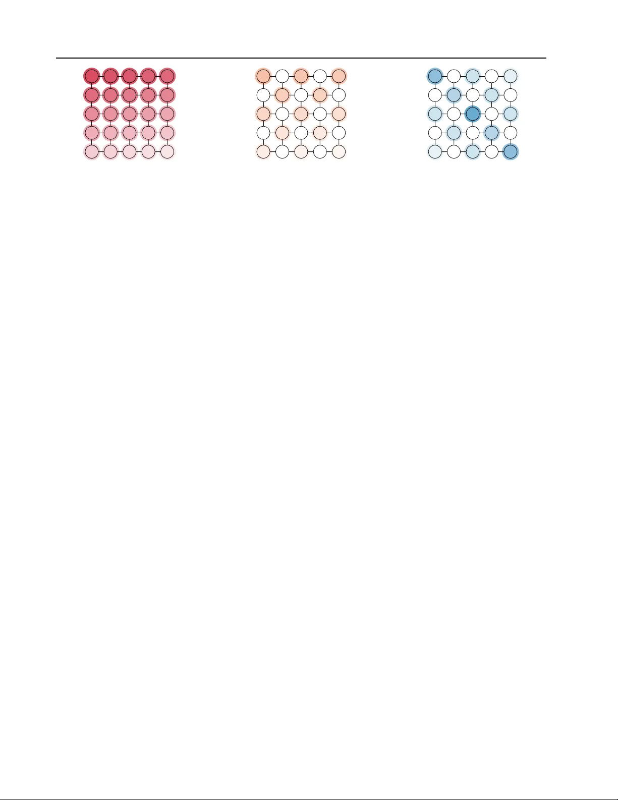
Selecting Optimal V ariable Order in A utor egr essiv e Ising Models Shiba Biswal 1 Marc V uffray 1 Andrey Y . Lokhov 1 Abstract Autoregressi v e models enable tractable sampling from learned probability distributions, b ut their performance critically depends on the variable or- dering used in the factorization via comple xities of the resulting conditional distributions. W e pro- pose to learn the Markov random field describing the underlying data, and use the inferred graphical model structure to construct optimized variable orderings. W e illustrate our approach on two- dimensional image-like models where a structure- aware ordering leads to restricted conditioning sets, thereby reducing model complexity . Numer- ical e xperiments on Ising models with discrete data demonstrate that graph-informed orderings yield higher-fidelity generated samples compared to naiv e v ariable orderings. 1. Introduction Autoregressi v e models are powerful decompositions widely used in modern AI architectures for producing exact samples from a learned representation of the data. Similar to the procedure used in a Bayesian network, ne w samples are generated using ancestral sampling : variables are visited in a topological order , and each v ariable x i is conditioned on the previously sampled “parent” v ariables x . Pr eprint. F ebruary 25, 2026. This in turn affects sample accuracy: good orderings sim- plify conditionals and reduce error propagation, while poor orderings force the model to learn unnecessarily complex dependencies. In the case where the joint probability distribution is rep- resented as a Marko v Random Field (MRF), this structure can be le veraged to construct optimized v ariable orderings. In general, the conditional p ( x i | x 1 , the number of terms in the parameterized conditional distribution ( 5 ) depends on the cardinality of its parent set P ar( k ) , and the order of interactions. W e reserve the symbol | · | to denote cardinality of a set. Suppose node k has d k := | Par( k ) | parents, and we parameterize the conditional distribution using polynomial interactions of degree at most O . Each interaction term in the exponent ( 5 ) is of the form x k Q j ∈ S x j , where S ⊆ Par( k ) . Restricting the total degree to be at most O implies that | S | ≤ O − 1 . Consequently , the number of interaction terms in v olving x k T := 1 + O − 1 X r =1  d k r  , where the +1 corresponds to the singleton interaction term corresponding to S = ∅ . If howe v er , O − 1 > d k , then the sum saturates to all subsets and then the number of terms equals 2 d k . W e define S ( O ) k = { S ⊆ Par( k ) : 0 ≤ | S | ≤ O − 1 } . The cardinality of this set is T . For a σ ( i ) , the conditional distrib ution of order at most O , can therefore be expressed as p  x σ ( i ) | x Par( σ ( i ))  = 1 Z σ ( i ) exp    x σ ( i ) X S ∈S ( O ) σ ( i ) ˜ θ σ ( i ) ,S Y j ∈ S x j    , (6) where ˜ θ σ ( i ) ,S denotes the effecti ve interaction coefficient associated with the monomial x σ ( i ) Q j ∈ S x j . Due to the reduction to the parent sets, the general decom- position ( 3 ) is simplified to: p ( x ) = p ( x σ (1) ) p  x σ (2) | Par( x σ (2)  p  x σ (3) | Par( x σ (3)  . . . p  x σ ( N ) | Par( x σ ( N )  . (7) using Markov pr operty and without any appr oximation. Now that we have defined conditionals entering in the au- toregressi v e decompositions, we will discuss methods for learning these conditional probabilities from data next. Learning conditionals in the autoregr essive decompo- sition. Given the choice of the permutation σ and the construction of the parent sets resulting in the final sim- plified autoregressi ve decomposition ( 7 ) , we discuss the method for learning of these conditionals from data. W e use the unconstrained version of the method kno wn as GRISE ( V uf fray et al. , 2020 ) that learns conditional probabilities of discrete undirected graphical models with higher-order interactions ( 6 ) . Suppose that we are giv en m independent and identically distributed (i.i.d.) samples, and denote the l th sample by x ( l ) = ( x ( l ) 1 , . . . , x ( l ) N ) . The GRISE estimate of parameters of conditional distrib utions in ( 6 ) for node i is obtained by solving the following minimization problem: ˜ S i = 1 m m X l =1 exp  − ˜ θ i x ( l ) i − x ( l ) i X S ∈S ( O ) i ˜ θ i,S Y j ∈ S x ( l ) j  , GRISE i : arg min ˜ θ i , { ˜ θ i,S } S ∈S ( O ) i ˜ S i . (8) W e do not discuss the details of this method further , b ut we notice that parameters of conditionals of order O can be consistently estimated in time O ( N O ) . 2.4. Selecting optimized ordering Learning of the Marko v random field structure. In the case where only data is initially av ailable, and the graph G = ( V , E ) is unknown, its structure can be learned using existing methods. For this purpose, we use an e xact and consistent method known as Re gularized Interaction Screen- ing Estimator (RISE) introduced in ( V uffray et al. , 2016 ) and with the hyper-parameters v alues prescribed in ( Lokhov et al. , 2018 ) without an y change. Given that this Ising model graph learning step is standard, we do not discuss the details of this method here. In all numerical examples below , we first learn the undirected graphical model structure associ- ated with the Marko v random field, and then study the effect of different v ariable orderings. Criterion for choosing optimized variable ordering. Once the MRF graph G = ( V , E ) is kno wn or has been learned, we propose the following strategy for selecting the optimized v ariable ordering for autoregressi v e decom- positions. F or a giv en sequence σ , we use the procedure abov e to define the parent sets based on the MRF edge set E . Denote d := max k d k = max k | Par( k ) | the maximum cardinality of the parent set in the autore gressiv e decom- position ( 7 ) . Let’ s also denote K the maximum number of conditionals with cardinality d appearing in ( 7 ) . According to the Theorem 2 in ( V uf fray et al. , 2020 ), these K con- ditionals are the hardest to learn: the number of samples required to guarantee a fixed error on the conditionals of the type ( 6 ) with degree d scale exponentially in d . Con versely , giv en a fixed number of samples m , we expect the largest error to impact conditionals with the maximum interaction order d . Therefore, we put forw ard a natural hypothesis: giv en a fix ed number of training samples m and comparing two permutations, (i) a permutation r esulting in a decom- position ( 7 ) with smaller d , and (ii) if d ar e the same for both permutations, a decomposition with smaller K should result in more accurately learned conditionals and hence 4 Selecting Optimal V ariable Order in Autor egr essive Ising Models 1 2 3 4 5 6 7 8 9 10 11 12 13 14 15 16 17 18 19 20 21 22 23 24 25 (a) Sequential Sequence 1 14 2 15 3 16 4 17 5 18 6 19 7 20 8 21 9 22 10 23 11 24 12 25 13 (b) Checkerboard Sequence 2 14 6 22 12 18 4 15 7 23 9 19 1 16 8 24 10 20 5 17 13 25 11 21 3 (c) Diagonal Sequence F igur e 2. Depiction of the three vari able order tra versals—sequential, check erboard, and diagonal —on a 5 × 5 lattice. Node shading indicates the relativ e selection order , from darker to lighter; identical shading denotes equal preference. Nodes without shading are selected after the shaded nodes and are not distinguished by the ordering. Node labels indicate one specific realization of the trav ersal. in a higher-quality autoregressiv e model. As a minor ad- ditional enhancement, choice of ordering can be further slightly optimized by selecting strongly correlated nodes and their parents in the lower -order conditionals, exploiting spatial correlation decay in maximum-order conditionals. W e rigorously test this hypothesis under control settings of i.i.d. samples in small models in the next section. 3. Results In this section, we validate our main hypothesis via numeri- cal experiments. For the first two sets of experiments, we consider the two-spin Ising model on square lattices with lattice side length L , so that the total number of nodes is N = L × L . W e focus on smaller test models because we can guarantee that we produce high-quality i.i.d. training samples for these models. W e then consider an application to real data produced by a quantum annealer . In all cases, we study two types of models. 1. Ferr omagnetic model: describes a system of spins x i ∈ {− 1 , +1 } with interactions fa vor alignment. W e fix θ i = 0 for all i ∈ V and θ i,j = +1 , for ( i, j ) ∈ E . Under this choice of parameters, the probability distribution ( 4 ) mostly concentrates on the two fully aligned configurations, namely x i = +1 for all i and x i = − 1 for all i . 2. Spin glass model : describes a system of spins x i ∈ {− 1 , +1 } with random couplings θ i,j ∈ {− 1 , 1 } or θ i,j ∈ [ − 1 , 1] , and with θ i = 0 . The randomness and competition between interactions lead to highly non- con v ex probability distribution ( 4 ) with many probabil- ity peaks. In all use cases (synthetic and real data), we first learn the MRF graph structure, and then use the learned structure to construct the structure-aware v ariable orderings. 3.1. Exact training samples: 5 × 5 square lattice In the first experiment, we consider a square lattice with L = 5 ( N = 25 ). The reason for considering this lattice size is that i.i.d. samples can be produced by brute force for any Ising model (including spin glasses) and we don’t ha ve to worry about the quality of the training data in this setup. W e fix the following three permutations σ (1) , . . . , σ ( N ) . • Sequence 1 (sequential order): nodes are selected se- quentially in row-wise order (see Figure 2a ). For a square lattice, this benchmark choice in volv es order K = O ( L 2 ) of conditionals with the max cardinality d = L . • Sequence 2 (checkerboard order): nodes are selected in the checkerboard pattern illustrated in Figure 2b . For a square lattice, this benchmark choice still in v olves or- der K = O ( L 2 ) of conditionals with the max cardinality d = L , but there are roughly twice less terms with the max cardinality (all remaining nodes in white have bounded cardinality 4 regardless of L ), and the terms in each condi- tional should be less correlated with each other . W e expect this choice to be better than the sequential benchmark. • Sequence 3 (diagonal trav ersal): this is the best opti- mized choice of variable ordering that we designed for a square lattice. The procedure is best understood by in- specting Figure 2c . The main idea is that conditioning on of the main diagonals directly makes the tw o parts of the lattice conditionally independent (inside this diagonal, we also optimize the sequence to minimize correlations). Then, the graph can be partitioned further by choosing next nodes in the diagonals, skipping one diagonal at a time as these result in nodes with bounded cardinality 4 regardless of L . This strategy still una voidably has terms with max cardinality d = L , but there are much fe wer of them compared to the first two strategies. The third permutation is constructed according to the hy- pothesis presented in Section 2.4 and serv es as our test case; we compare its sampling error against the other two permutations that serv e as baselines. W e e xpect the test permutation to be optimized compared to the other two. In realistic applications, learning of conditionals in the au- toregressi v e decomposition ( 7 ) will hav e two sources of error: (i) statistical error from finite number of training sam- ples; (ii) systematic error from a reduced interaction order 5 Selecting Optimal V ariable Order in Autor egr essive Ising Models (a) Ferromagnetic Model (b) Spin glass Model F igur e 3. Number of training data samples M l versus sampling error ε ( 9 ) for both ferro and spin glass Ising models with conditional order O = 6 . The number of generated samples M s = 10 5 . Error bars are one standard deviation ov er 20 independent training data sets. approximating the conditionals for large models. W e use the small N = 25 model to study the impact of each of these factors separately . Learning models of fixed order using data samples. In this set of experiments, we study how learning the con- ditional distributions in ( 6 ) from a finite number of data samples affects the resulting sampling error . Data Generation: W e generate 20 independently sampled datasets of size M l from a 5 × 5 square lattice for both the ferromagnetic and spin glass models. In the latter case, each dataset corresponds to a distinct instance of the model in which the edge couplings θ i,j ∈ {− 1 , 1 } are drawn uni- formly at random. W e v ary the number of training samples M l ov er the set { 0 . 5 × 10 5 , 2 . 5 × 10 5 , 5 × 10 5 , 10 × 10 5 , 20 × 10 5 } , Learning Conditional Distributions: The parameters in ( 6 ) for each sequence are learned using the GRISE estimator defined in ( 8 ) . Since the underlying graph is a 5 × 5 square lattice, the maximum cardinality of P ar( i ) ov er all i ∈ V and for all three sequences considered is at most 5. Con- sequently , the order of the model, denoted by O in ( 6 ) , is fixed to 6 , accounting for a fully-expressible conditionals with interactions up to order six together with the bias term. Sampling: W e fix the number of samples generated from the learned models to M s = 10 5 , using the sampling procedure described in ( 7 ) . In Figure 3 , we present log - log plots of M l against the sampling error , defined to be the difference in the first two moments of the empirical distrib ution ˆ p := 1 M s P M s l =1 δ x ( l ) and the true distribution p ( 4 ): ε = ( ∥ E ˆ p [ x ] − E p [ x ] ∥ 2 + ∥ Cov ˆ p ( x ) − Cov p ( x ) ∥ F ) 1 2 , (9) where ∥ · ∥ 2 , ∥ · ∥ F are the 2 -norm and the Frobenius norm, respectiv ely . The vertical error bars represent the single error standard deviations o v er the 20 sampled datasets. Discussion: As shown in Figure 3 , the sampling error de- creases as M l increases, as expected, and saturates for larger values of M l . T o understand the saturation, we additionally plot the baseline sampling error arising solely from finite sampling, obtained by drawing M s samples directly from the ground-truth distribution ( 4 ) (no model can produce bet- ter error than baseline due to finite samples). For the spin glass model, the baseline is averaged over the 20 random instances of the coupling realizations. In both model types, howe ver , Sequence 3—the diagonal trav ersal—yields lower sampling error than the other two sequences; this improv ement is particularly pronounced in the ferromagnetic case (Figure 3a ). In contrast, the spin glass model (Figure 3b ) appears less sensitive to the choice of variable ordering, lik ely due to the hardness of sampling intrinsic to frustrated spin-glass models. Still, there is a clear separation (larger than the error bars) between the sampling error curves e v en in the spin-glass case. Learning models of v arying order using the true Distri- bution. In this set of experiments, we study how order of the model, denoted by O in ( 6 ) , aff ects the sampling error in the ferromagnetic case. Moreov er , the conditionals are learned from the true distribution, eliminating the error that stems from finite training samples. Learning conditional distributions: T o isolate the ef fect of model order from errors arising due to finite training data, we learn the conditional distrib utions in ( 6 ) , for each se- quence, directly from the true probability distribution ( 4 ) . Specifically , we enumerate all 2 25 configurations x and com- pute their exact probabilities p ( x ) , which are then used in place of empirical frequencies in the GRISE objecti ve ( 8 ) . T o learn the conditional distributions, we use model of or - ders that vary o ver O ∈ { 2 , 4 , 6 } , and hence approximating the conditional probabilities in the decomposition ( 7 ). Sampling: F or each sequence and each model order, we generate M s samples from the learned autoregressi ve model, with M s ∈ { 1 × 10 5 , 2 . 5 × 10 5 , 5 × 10 5 , 10 × 10 5 } . In Figure 4 , we present the log - log plots of M s verses the sampling error (the difference in the first two moments of the empirical and the true distribution). The reported results are averaged over 50 independent sampling runs, and the vertical error bars indicate the respectiv e standard deviation. 6 Selecting Optimal V ariable Order in Autor egr essive Ising Models (a) Order = 2 (b) Order = 4 (c) Order = 6 F igur e 4. Number of generated samples M s versus sampling error ε ( 9 ) for a ferromagnetic Ising model with different conditional orders O ∈ { 2 , 4 , 6 } , where the conditionals are learned from the ground-truth distribution p . Error bars indicate one standard deviation over 50 independently generated sample sets. Discussion: As shown in Figure 4 , the sampling error de- creases with increasing M s for all model orders. In all cases, Sequence 3 yields the lowest sampling error , validating our hypothesis. Interestingly , increase of the model order in learning of conditionals does not lead to a significant im- prov ement in performance due to small value and impact of higher-order terms for the models of ferromagnetic type. 3.2. High-quality training samples: 10 × 10 ferro model W e expect the effect already visible on models of size N = 25 to be pronounced in larger models as well. It is howe v er harder to perform numerical e xperiments under controlled setting as a reliable production of i.i.d. samples becomes an issue. Luckily , high-quality samples can still be obtained for specific models such as ferromagnetic models without local field. This is precisely the type of models that we study in this second experiment. W e consider the same three permutations as in the previous section, and study the combined effect of the reduced model order in learning of conditionals (due to computational comple xity) and the finite number of training samples on the sampling error . Data generation. W e generate data using a Markov chain Monte Carlo algorithm known as Gibbs sampling. For this specific model, we can use a special trick to av oid issues with conv ergence of Markov chains based on the f act that we know two configurations maximizing the probability den- sity . W e thus run two independent Marko v chains initialized at x = (1 , 1 , . . . , 1) and x = ( − 1 , − 1 , . . . , − 1) , discard an initial b urn-in period, and combine an equal number of samples from each chain to form the final dataset. T raining datasets of size M l ∈ { 0 . 5 × 10 5 , 2 . 5 × 10 5 , 5 × 10 5 } are generated. In the ferromagnetic case, where the distrib u- tion is dominated by two magnetized modes, this procedure ensures that both modes are adequately sampled and elimi- nates bias due to slow mixing between them. Learning conditional distributions. For each sequence, we learn the parameters of the conditional model ( 6 ) using the Interaction Screening Estimator ( 8 ) . In this experiment, we fix the model order to O = 2 and O = 4 . Sampling. The number of generated samples is fixed to M s = 10 5 . In Figure 5 , we report log - log plots of the sampling error as a function of M l . The sampling error is av eraged ov er 50 independently generated sample sets, and error bars correspond to one standard deviation. (a) Order = 2 (b) Order = 4 F igur e 5. Number of training data samples M l versus sampling error ε ( 9 ) for ferro Ising model with model orders O ∈ { 2 , 4 } . The number of generated samples M s = 10 5 . Error bars indicate one standard deviation o ver 20 independent training data sets. Discussion. As shown in Figure 5 , the model order in ( 6 ) plays a more pronounced role in this larger system. Com- pared to the 5 × 5 lattice, the increased system size leads to more complex conditional dependencies, making the e x- pressivity of the conditional model more consequential. In particular , the sampling error saturates more rapidly for the lower -order model ( O = 2 ) than for the higher-order 7 Selecting Optimal V ariable Order in Autor egr essive Ising Models (a) Sequential Se- quence (b) Cross Sequence F igur e 6. Depiction of two sampling sequences for the D-W ave dataset. The top panel illustrates the sublattice-lev el selection, while the bottom panel sho ws the selection order of nodes within each sublattice. Node shading indicates selection order . F igur e 7. Number of generated samples M s versus sampling error ε ( 9 ) for the D-W av e spin glass Ising model with model order O = 3 , where the conditional distributions are learned from M l = 5 × 10 5 . Error bars indicate one standard deviation o ver 20 independently generated sample sets. model ( O = 4 ), suggesting that the lo wer -order model becomes capacity-limited at smaller training sizes. In con- trast, the higher -order model continues to benefit from ad- ditional training data. Moreover , across both model orders, Sequence 3 consistently yields the lowest sampling error , highlighting the adv antage of structure-informed diagonal trav ersals in lar ger , ordered lattices. 3.3. Real data use case: D-W ave Dataset In this experiment, we ev aluate the effect of v ariable permu- tations on the sampling algorithm in a non-synthetic setting, using data produced by a D-W ave 2X quantum annealer . The publicly a v ailable dataset ( Lokho v et al. , 2018 ) consists of recorded samples of 62 qubits (i.e., |V | = 62 ) together with their empirical frequencies. The qubits are arranged on a non-square lattice, see Figure 6 the connectivity can be viewed approximately as a 9 × 9 lattice in which each node is itself replaced by a small, sparsely connected sub- graph resembling a 4 × 2 lattice; sev eral qubits are broken, represented by the missing edges in see Figure 6 , which represents another interesting aspect of this dataset due to a connectivity irre gularity . The underlying probability distrib ution is unkno wn. How- ev er , the system is known to be well approximated by an Ising model with both pairwise couplings θ i,j and local fields θ i , with parameters drawn uniformly from the range [ − 2 . 0 , − 0 . 25] ∪ [0 . 25 , 2 . 0] . Consequently , this instance cor - responds to a spin glass model. Learning the graph topology . Learning the graph topology . W e first reconstruct the underlying MRF graph topology as explained in the methods section. Based on the recov ered edge weights, we then consider the following two sampling sequences: sequential depicted in Figure 6a (similar to the baseline used in square lattice e xperiments), and cross order depicted in Figure 6b (similar to the optimized variable order in the synthetic experiments). Learning conditional distributions. W e fix the model order to O = 3 , and learn the corresponding conditional distri- butions for both sequences using the Interaction Screening Estimator ( 8 ) and the av ailable data samples. Sampling. For each learned model, we generate M s samples with M s ∈ { 1 × 10 5 , 2 . 5 × 10 5 , 5 × 10 5 , 10 × 10 5 } . W e av erage results ov er 50 independent sampling runs, and use the same error metric corresponding to two moments of the distribution. Discussion. Results in Figure 7 show a similar trend to spin-glass model in the synthetic experiments: the sampling error decreases with increasing M s , as expected, and small sensitivity to the choice of v ariable ordering. This behavior is consistent with the strongly disordered nature of the D- W ave dataset. Still, it is interesting to see that the structure- aware cross order consistently sho ws an adv antage ov er the naiv e ordering, supporting the general finding of this work. 4. Conclusions and future w ork In this work, we deliberately focused on small-scale mod- els where exact or well-controlled sampling procedures are av ailable, allowing us to isolate and analyze the effect of variable ordering in autore gressi ve sampling. Even in these small models, we observe clear and systematic differences in sampling performance across orderings. These ef fects are expected to become more pronounced for larger systems, where conditioning complexity and error accumulation grow with system size. W e also restricted our study to explicit parametric forms in order to quantify the impact of model expressi vity on the performance of models with different variable orderings. Future work should benchmark the con- clusions from this work on large models and datasets, using neural-net representations for the conditionals ( Jayakumar et al. , 2020 ) and exploring the extension to continuous v ari- ables. The code reproducing all results in this work is av ailable at Github . 8 Selecting Optimal V ariable Order in Autor egr essive Ising Models Impact Statement This paper presents work whose goal is to advance the field of Machine Learning. There are many potential societal consequences of our work, none which we feel must be specifically highlighted here. References Białas, P ., Korc yl, P ., and Stebel, T . Hierarchical autoregres- siv e neural networks for statistical systems. Computer Physics Communications , 281:108502, 2022. Biazzo, I., Wu, D., and Carleo, G. Sparse autoregressi v e neural networks for classical spin systems. Mac hine Learning: Science and T echnolo gy , 5(2):025074, 2024. Black, S., Biderman, S., Hallahan, E., Anthon y , Q., Gao, L., Golding, L., He, H., Leahy , C., McDonell, K., Phang, J., et al. Gpt-neox-20b: An open-source autoregressi ve language model. In Proceedings of BigScience Episode# 5–W orkshop on Challenges & P erspectives in Creating Lar ge Language Models , pp. 95–136, 2022. Brown, T ., Mann, B., Ryder, N., Subbiah, M., Kaplan, J. D., Dhariwal, P ., Neelakantan, A., Shyam, P ., Sastry , G., Askell, A., et al. Language models are few-shot learners. Advances in neural information pr ocessing systems , 33: 1877–1901, 2020. Del Bono, L. M., Ricci-T ersenghi, F ., and Zamponi, F . Per- formance of machine-learning-assisted monte carlo in sampling from simple statistical physics models. Physi- cal Revie w E , 112(4):045307, 2025. Germain, M., Gregor , K., Murray , I., and Larochelle, H. Any-order autore gressi ve models for approximate infer - ence. In Pr oceedings of the 32nd International Confer- ence on Machine Learning (ICML) , 2015a. Germain, M., Gregor , K., Murray , I., and Larochelle, H. Made: Masked autoencoder for distribution estimation. In International conference on machine learning , pp. 881– 889. PMLR, 2015b. Jayakumar , A., Lokhov , A., Misra, S., and V uffray , M. Learning of discrete graphical models with neural net- works. Advances in Neural Information Pr ocessing Sys- tems , 33:5610–5620, 2020. Kitson, N. K. and Constantinou, A. C. Eliminating variable order instability in greedy score-based structure learning. In International Confer ence on Probabilistic Graphical Models , pp. 147–163. PMLR, 2024a. Kitson, N. K. and Constantinou, A. C. The impact of variable ordering on bayesian network structure learn- ing. Data Mining and Knowledge Discovery , 38(4):2545– 2569, 2024b. Kliv ans, A. and Meka, R. Learning graphical models using multiplicativ e weights. In 2017 IEEE 58th Annual Sym- posium on F oundations of Computer Science (FOCS) , pp. 343–354. IEEE, 2017. Lokhov , A. Y ., V uffray , M., Misra, S., and Chertkov , M. Optimal structure and parameter learning of ising mod- els. Science Advances , 4(3):e1700791, 2018. doi: 10. 1126/sciadv .1700791. URL https://www.science. org/doi/abs/10.1126/sciadv.1700791 . Papamakarios, G., Pavlak ou, T ., and Murray , I. Masked autoregressi v e flo w for density estimation. Advances in neural information processing systems , 30, 2017. Shi, C., Xu, M., Zhu, Z., Zhang, W ., Zhang, M., and T ang, J. Graphaf: a flo w-based autoregressi v e model for molec- ular graph generation. arXiv preprint , 2020. Uria, B., C ˆ ot ´ e, M.-A., Gregor , K., Murray , I., and Larochelle, H. Neural autoregressi ve distribution esti- mation. Journal of Machine Learning Resear ch , 17(205): 1–37, 2016. V uf fray , M., Misra, S., Lokhov , A., and Chertkov , M. Inter- action screening: Efficient and sample-optimal learning of ising models. Advances in neural information pr ocess- ing systems , 29, 2016. V uf fray , M., Misra, S., and Lokhov , A. Efficient learning of discrete graphical models. Advances in Neural Informa- tion Pr ocessing Systems , 33:13575–13585, 2020. Y ou, J., Y ing, R., Ren, X., Hamilton, W ., and Lesko vec, J. Graphrnn: Generating realistic graphs with deep auto- regressi v e models. In International confer ence on ma- chine learning , pp. 5708–5717. PMLR, 2018. 9