ODEBrain: Continuous-Time EEG Graph for Modeling Dynamic Brain Networks

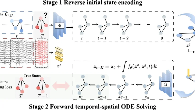
Published as a conference paper at ICLR 2026 O D E B R A I N : C O N T I N U O U S - T I M E E E G G R A P H F O R M O D E L I N G D Y N A M I C B R A I N N E T W O R K S Haohui Jia ♠ , Zheng Chen ♣ , † , Lingwei Zhu ♢ , Rikuto Kotoge ♣ , Jathurshan Pradeepkumar ♡ , Y asuko Matsubara ♣ , Jimeng Sun ♡ , Y asushi Sakurai ♣ , T akashi Matsubara ♠ ♠ Information Science and T echinology , Hokkaido Univ ersity , Japan ♣ SANKEN, The Univ ersity of Osaka, Japan ♢ Great Bay Univ ersity , China ♡ Department of Computer Science, Univ ersity of Illinois Urbana-Champaign, USA † Corresponding author: chenz@sanken.osaka-u.ac.jp A B S T R A C T Modeling neural population dynamics is crucial for foundational neuroscientific research and various clinical applications. Con ventional latent variable methods typically model continuous brain dynamics through discretizing time with recur- rent architecture, which necessarily results in compounded cumulativ e prediction errors and failure of capturing instantaneous, nonlinear characteristics of EEGs. W e propose ODEBRAIN , a Neural ODE latent dynamic forecasting frame work to ov ercome these challenges by integrating spatio-temporal-frequenc y features into spectral graph nodes, followed by a Neural ODE modeling the continuous latent dynamics. Our design ensures that latent representations can capture stochastic variations of comple x brain states at any giv en time point. Extensive e xperiments verify that ODEBRAIN can improve significantly ov er existing methods in fore- casting EEG dynamics with enhanced robustness and generalization capabilities. 1 I N T R O D U C T I O N Modeling dynamic acti vity in brain networks or connecti vity using electroencephalograms (EEGs) is crucial for biomarker discovery ( Rolls et al. , 2021 ; Jones et al. , 2022 ) and supports a wide range of clinical applications ( K otoge et al. , 2024 ; Pradeepkumar et al. , 2026 ). T emporal graph networks (TGNs), which integrate temporally sequential models (such as RNNs) with graph neural networks (GNNs), hav e recently emerged as a promising approaches ( T ang et al. , 2022 ; Ho & Armanfard , 2023 ; Delav ari et al. , 2024 ; Li et al. , 2024 ). These methods represent multi-channel EEGs as graphs, where GNNs capture spatial dependencies and sequential models capture fine-grained temporal dy- namics, thereby providing mechanistic insights into gradual e volution of brain networks. Howe ver , a critical yet overlook ed problem remains: existing methods transform EEGs into fixed, discrete time steps, which conflicts with the inherently continuous nature of dynamic brain networks. Such discretization imposes rigid windowing assumptions and prevents models from capturing the unfolding time-course dynamics or irre gular transitions in brain networks, as in Figure 1 . This paper aims to tackle this issue by de veloping a novel method that models EEGs in an e xplicitly continuous manner , while lev eraging Neural Ordinary Differential Equations (NODEs) ( Chen et al. , 2018 ). In contrast to RNN-based sequential models, which discretize time into fixed steps, NODEs parameterize the deriv ative of the hidden state and integrate it continuously over time ( Park et al. , 2021 ). This formulation provides a principled method to model the dynamical ev olution of neural activity ( Hu et al. , 2024 ) and has been studied across domains ( Hwang et al. , 2021 ), including brain imaging ( Han et al. , 2024 ). In this paper , we study a nov el and critical problem: modeling dynamics brain networks with NODEs to learn informativ e continuous-time representations from EEGs. This remains a unexplored and non-tri vial task, and we focus on two main challenges: ( i ) Effective spatiotemporal modeling for ODE initialization. NODEs critically depend on the quality of their initial conditions, because the ODE solver propagates trajectories starting from this 1 Published as a conference paper at ICLR 2026 Forecasting for exploration of neuronal population dynamics Channel Continuous forecasting (ODE-based) Latent state Discrete forecasting (recurrent-based) Time Continuous EEG recordings Observed Forecasting Figure 1: (Left) Continuous EEG real-time neuronal activity recordings. (Mid) Recurrent-based methods employ discrete modeling. (Right) ODE provi des a continuous representation for forecast- ing neuronal population dynamics. initialization. Accordingly , a poor initialization propagates errors and destabilizes long-term dy- namics. Howe ver , EEG signals are inherently noisy and stochastic, which makes learning robust spatiotemporal representations of brain networks particularly challenging. Therefore, designing an initialization that captures meaningful spatiotemporal structures is essential for stable ODE integra- tion and effecti ve do wnstream learning. ( ii ) Accurate trajectory modeling. Trajectory modeling is essential for NODEs, as their strength lies in learning continuous latent dynamics rather than discrete predictions. Unlike con ventional time- series data, which often exhibit stable patterns such as periodicity or long-term trends ( Kl ¨ otergens et al. , 2025 ), EEG signals are highly v ariable, which makes trajectory learning particularly challeng- ing. Thus, a major challenge is to constrain and preserve meaningful trajectories in the latent space so that NODEs can accurately capture the continuous dynamics of EEGs. In this paper , we introduce a new continuous-time EEG Graph method, ODEBRAIN , based on the NODE, for modeling dynamic brain networks. T o address the above challenges, we first propose a dual-encoder architecture to provide effecti ve initialization for NODEs. One encoder captures deter - ministic frequency-domain observations to model brain networks, whereas the other integrates raw EEG representations to retain stochastic characteristics. This combination yields robust spatiotem- poral features for initializing the ODE solv er . Second , we introduce a trajectory forecasting decoder that maps latent representations obtained from NODE solutions back to graph structures. There- after , a multistep forecasting loss function was applied to explicitly predict future brain networks at different time steps. This design enables direct trajectory modeling of dynamic brain networks and enhances accurac y . Third , beyond modeling, we are the first to propose the use of the gradient field of NODEs as a metric to quantify EEG brain network dynamics. Herein, we also conduct a case study on seizure data to illustrate the clinical interpretability of this method. • New problem F ormulation. T o the best of our kno wledge, we are the first to e xplicitly formulate EEG brain networks as a continuous-time dynamical system, where the brain network is repre- sented as a sequence of time-varying graphs whose latent dynamics are governed by a NODE. This perspective differs from prior approaches based on recurrent models, which model gradual state transitions in a discrete-time framew ork rather than in a principled continuous-time manner . • Novel Method. W e dev elop the ODEBRAIN frame work that integrates three key components. It first combines deterministic graph-based features with stochastic EEG representations to produce a robust initial state. Then an explicit trajectory forecasting decoder with multi-step forecast- ing loss hat models temporal–spatial dynamics continuously , enabling principled forecasting of ev olving brain networks. • Comprehensive Evaluation. W e demonstrate strong performance across benchmarks and pro- vide retrospective clinical case studies highlighting the interpretability . Our ODEBRAIN outper- forms all baselines on the TUSZ dataset, achie ving 6.0% and 8.1% improv ements in F1 and A CC, respectiv ely . On the TU AB, ODEBRAIN consistently achiev es best performance, such as 1.2% improv ed F1 and 2.4% improved A UR OC. Moreover , we further ev aluate the learned field and its clustering to rev eal the dynamic behaviors (varying speed and direction) between seizure and normal states, and achieving 12.0% impro vement for brain connecti vity prediction. 2 R E L A T E D W O R K S T emporal graph methods f or modeling EEG dynamics. 2 Published as a conference paper at ICLR 2026 GNNs hav e emerged as powerful method for effecti vely capturing spatial dependencies and rela- tional structures in the analysis of brain networks ( Li , 2022 ; Y ang & Hong , 2022 ; Kan et al. , 2023 ). Specifically , EEG-GNN performs a learnable mask to filter the graph structure of EEG for cogniti ve classification tasks ( Demir et al. , 2021 ). ST -GCN formulates the connectivity of spatio-temporal graphs to capture non-stationary changes ( Gadgil et al. , 2020 ). T ang et al. ( 2022 ) have introduced the DCRNN approach for graph modeling, setting a new standard for SOT A in seizure detection and classification tasks. Follo wing this, GRAPHS4MER ( T ang et al. , 2023 ) enhanced the graph structure and integrated it with the MAMB A framework to improve long-term modeling capabili- ties. AMAG ( Li et al. , 2024 ) forecasting method has been proposed to ef fectively capture the causal relationship between past and future neural activities, demonstrating greater efficienc y in modeling dynamics. More recently , EvoBrain in vestigates the expressiv e power of TGNs in integrating tem- poral and graph-based representations for modeling brain dynamics ( K otoge et al. , 2025 ). Howe ver , these studies rely on discrete modeling, and may lead to suboptimal representation of continuous dynamics of brain networks. Differential equations for brain modeling. Modeling brain function as lo w-dimensional dynam- ical systems via differential equations has been a long-standing direction in neuroscience ( Church- land et al. , 2012 ; Mante et al. , 2013 ; Vyas et al. , 2020 ), and nonlinear EEG analysis for brain activity mining ( Pijn et al. , 1997 ; Xue et al. , 2016 ; Lehnertz et al. , 2003 ; Lehnertz , 2008 ; Mercier et al. , 2024 ). Recently , Neural ODEs (NODEs) formulate dynamical systems by parameterizing deriv a- tiv es with neural networks and have shown impressive achiev ements across diverse fields ( Fang et al. , 2021 ; Hwang et al. , 2021 ; Park et al. , 2021 ). In BCI and epilepsy modeling, controllable formulations and fractional dynamics provide important theoretical foundations for modeling brain dynamics ( Gupta et al. , 2018b ; Tzoumas et al. , 2018 ; Lu et al. , 2021 ; Martis et al. , 2015 ; Lepeu et al. , 2024 ). In latent-variable dynamics models, the EEG and neuronal processes are described as fractional dynamics ( Gupta et al. , 2019 ; 2018a ; Y ang et al. , 2019 ; 2025 ). In neuroscience, Kim et al. ( 2021 ) learn neural activities by modeling the latent evolution of nonlinear single-trial dy- namics with Gaussian processes from neural spiking data. Hu et al. ( 2024 ) propose using a smooth 2D Gaussian kernel to represent spikes as latent variables and describe the path dynamics with lin- ear SDEs. Another study ( Cai et al. , 2023 ) demonstrates robust performance in neuroimaging by combining biophysical priors with NODEs, starting from predefined cognitiv e states. ( Chen et al. , 2024 ) have sho wn the advantage of graph ODE by modeling continuous-time propagation for EEG emotion task. Han et al. ( 2024 ) further illustrate that integrating spatial structure with NODEs can effecti vely facilitate the modeling of neuroimaging dynamics, ev en in the presence of missing data. Howe ver , these studies focus on imaging data or neuronal feature engineering, while data-driv en modeling of brain networks with fractional dynamics from EEGs remains underexplored. 3 P R E L I M I N A RY A N D P RO B L E M F O R M U L A T I O N Neural Ordinary Differential Equations. NODEs ( Chen et al. , 2018 ) provide a framew ork for modeling continuous-time dynamics by parameterizing the deriv ativ e of a hidden state using neural networks. Intuitiv ely , NODEs solve the trajectory of the hidden state continuously at any arbitrary time τ , rather than restricting updates to fixed discrete steps ∆ t in RNNs. Specifically , the hidden dynamics are computed via an adaptiv e numerical ODE solver: z ( t + 1) ≃ ODEsolver ( z 0 , f θ ) = z 0 + Z t +1 t f θ ( t, z t ) dt, (1) where f θ is a continuous, differentiable function parameterized by a neural network. This formula- tion yields a unique continuous trajectory z ( t ) ov er an interval [ t 0 , t 0 + τ ] . Intuition in Modeling EEG Dynamics. Con ventional sequential models, such as RNNs, ha ve been a standard tool for modeling EEG. Howe ver , they implicitly assume that time can be discretized into fixed steps and that state transitions, such as the onset of a seizure, must occur exactly at these steps ( K otoge et al. , 2025 ). While this assumption simplifies the computation, it poorly matches the reality of EEG, where brain activity evolv es continuously and transitions can occur at arbitrary points in time. In contrast, NODEs address this limitation by modeling EEG dynamics through a continuous function f θ whose integration yields smooth latent trajectories. W ithin this framew ork, discrete EEG signals recorded at sampling intervals are treated as observations sampled from an underlying continuous process R f θ ( t ) dt . This perspective allows NODEs to capture both gradual oscillatory 3 Published as a conference paper at ICLR 2026 ...... ...... Input gra phs Stage 1 Reverse initial state encoding Stage 2 Forward temporal-spatial ODE Solving ... C ... T rue States Multi-steps forecasting loss Figure 2: Continuous neural dynamics modeling via ODEBRAIN with graph forecasting. In stage 1, multi-channel EEG signals are encoded into spectral graph snapshots and fused with raw features to construct noise-robust initial states for ODE integration, predicting future spectral graphs. In stage 2, ODEBRAIN propagates latent states through time, generating dynamic field f that captures continuous trajectories. Finally , future graph node embeddings are obtained by z T and compared with the ground-truth graph nodes. rhythms and abrupt transitions in neural activity , thereby pro viding a more faithful representation of the EEG brain dynamics. Howe ver , applying the NODE to EEG is non-trivial, and we recognize two questions needing to be answered: 1. Robust initialization z 0 against transients and stochasticity in EEGs. NODE requires a well- cablibrated starting condition z 0 to effecti vely forecast future behavior . This is because EEGs are highly stochastic, or even chaotic to an extent. Their key features are transient and may appear without any preindicator ( Chen et al. , 2022 ). W ithout proper initialization z 0 as a guide, the integration of the model f θ ov er time alone cannot accurately forecast future states. 2. Meaningful objectives of f θ ( t, z t ) to capture the underlying EEG dynamics. Standard NODE training typically relies on regression-lik e objectives aimed at forecasting future states. A key challenge lies in identifying which representations best capture the underlying neural dynamics, so that f θ ( t, z t ) is guided to ward modeling the true ev olution of brain networks rather than only surface-le vel predictions. For example, in seizure analysis, the model must also learn to discern not only seizure but also an y leading states that herald an impending seizure ( Li et al. , 2021 ). Problem Statement (Modeling Dynamic Brain Networks). Giv en the observed EEG up to time t , denoted as X ≤ t , the objectiv e is to model the dynamics of the brain network and forecast their future ev olution. The predicted dynamics act as representations of brain states, enabling the distinction between conditions such as seizure and non-seizure. Following prior work ( T ang et al. , 2022 ; Chen et al. , 2025 ), we represent the brain as a graph and aim to dev elop an EEG-based NODE ( Ω ) to predict a sequence of time-varying graphs: G t +1: t + K = { X t +1 , . . . , X t + K } = Ω  z 0 , f θ ( G 1: t )  . (2) Over the next K steps graph, where G 1: t denotes the observed brain networks up to time t , and G t +1: t + K represents the predicted dynamic brain networks. These graphs characterize dynamic brain networks, but this problem poses two key challenges: (i) obtaining a robust initialization z 0 that can resist the transient and stochastic nature of EEGs; and (ii) defining an objectiv e for f θ that faithfully captures the underlying neural dynamics. 4 Published as a conference paper at ICLR 2026 4 M E T H O D O L O G Y Figure 2 shows the system overvie w of ODEBRAIN . Specifically , graph representations are obtained from each EEG segment (Section A.2 ), entering stage 1: attaining re verse initial state encoding z g and temporal encoding z s (Section 4.1 ). Stage 2 consists of a Neural ODE that takes as input z g , z s (Section 4.2 ). Finally , forecasting loss between ODE output and ground truth is computed. 4 . 1 S TAG E 1 : R E V E R S E I N I T I A L S T ATE E N C O D I N G Spectral Node Embedding. Pre vious discrete forecasting studies have shown that the capacity to estimate future neural dynamics depends on past activity in ( Li et al. , 2024 ). W e also define this forecasting paradigm within our ODEBRAIN . Intuiti vely , both the latent initial state z 0 and the field f , i.e., dz ( t ) dt are described by encoding the past observation G i, ≤ t to govern the latent continuous ev olution. The works of ( Rubanov a et al. , 2019 ; Chen et al. , 2018 ) suggest that the construction of an effecti ve latent initial state requires an autoregressiv e model capable of jointly extracting both the initial condition and the latent ev olution. Accordingly , we introduce a graph state descriptor Φ : R d 7→ R m that represents latent graph states z g ∈ R m using the autoregressi ve and graph network modules. Specifically , given the observations until now G i, ≤ t as input, we perform a sequence represen- tation for the node and edge attributes. For node embeddings, node ev olution is computed by h n i = GR U node ( X i, ≤ t ) where V i, ≤ t denote the spectral attribute sequences of node i and X i, ≤ t the spectral intensity . Similarly , for edge, the attribute sequences are defined from adjacency ma- trices by h e ij = GR U edge ( A ij, ≤ t ) . The resulting node and edge embeddings are integrated into an aggregated graph structure G = ( h n i,t , h e ij,t ) to be learned by a GNN to capture the spatial depen- dency across epochs: z g = GNN  h n i , h e ij  . The forward process of Φ captures both the epoch variations between frequenc y bands and explicit channel correlations. T emporal Embedding with Stochasticity . Accurate modeling of the temporal e volution of EEG signals is crucial because neural dynamics inherently e xhibits nonuniform temporal fluctuations and asynchronous activ ations across channels. Although the graph descriptor Φ effecti vely captures the ev olution of the node and edge attributes, STFT segments the EEG signals by constant windows, which inevitably disrupts the continuous temporal correlation between the ra w EEG observations. Pr oposed temporal-spatial ODE-RK4 function ... ... (a) (b) Adaptive neural dynamics Stochastic regularization Figure 3: The full structure of the temporal- spatial ODE solving. (a)RK-4 step numerical solver . (b) Procedure of temporal-spatial f θ . Moreov er, fully deterministic latent representations lack the flexibility necessary to ef fectively repre- sent transient motions of EEG as analyzed in Sec- tion 3 . Conv ersely , introducing controlled random- ness into temporal embeddings serves as a natural regularization strategy , effecti vely increasing the ro- bustness and preventing premature con vergence to suboptimal. Here, we apply the temporal descriptor Ψ : R T × L 7→ R c , c ≪ m to quantify the random- ness of the raw EEG epochs across N channels into z s ∈ R c . Giv en EEG segments X from N channels within a sliding windo w length L , we define stochas- tic temporal embedding as z s = Ψ( X T × L, ≤ N ) . The controlled stochasticity further acts as a form of la- tent space regularization, enhancing generalization and robustness to noise in EEG data collection. 4 . 2 S TAG E 2 : F O RW A R D T E M P O R A L - S PA T I A L O D E S O L V I N G Depending on the above encoding process, we define the initial state z 0 = [ z s , z g ] with Φ ◦ Ψ 7→ R m + c , which summarizes stochastic temporal variability and deterministic spectral connectivity , respectiv ely . Given the initial state z 0 ∈ R m + c , the general approach models the ODE vector field following the classical neural netw ork solution f θ with residual connection as: d z ( t ) ≡ f θ ( z ( t ) , t ; Θ ) dt, z 0 = [ z s , z g ] , t ∈ [ t + 1 , t + K ] (3) 5 Published as a conference paper at ICLR 2026 where f θ : R m + c 7→ R m + c represents a vector field to capture complicated dynamics and its continuous ev olution is gov erned by f θ with the learnable Θ across the entire epoch sequences. Howe ver , this introduces the challenge of optimizing the deep network-based f θ ov er highly variable EEG states, making large solv er errors. Considering the deep architecture-based multi-step numerical solver design ( Lu et al. , 2018 ; Oh et al. , 2024 ) and logic gating interaction of brain dynamics ( Goldental et al. , 2014 ), we design a temporal-spatial ODE solution to incorporate the initial state z 0 for additive and gate operations as shown in Figure 3 . In addition, we further introduce an adaptiv e decay component conditioned on the stochastic temporal state z s , to adjust the vector field f θ , accounting for the complexity and dynamic nature of the brain as a system. As sho wn in Figure 3 (b), the f θ used in the proposed ODE function is computed as follows: f θ ( z 0 ) = ( g ( z 0 ) + 1 ) ⊙ h ( z 0 ) − λ  z s  z 0 , z 0 = [ z s , z g ] , (4) where ⊙ represents the element-wise multiplication. Initially , the vector field is computed by the general residual block h ( z 0 ) and updated by a gated vector field with a sigmoid function σ as: g ( z 0 ) = σ ( W g z 0 + b g ) ∈ (0 , 1) m + c , (5) which provides state-adaptiv e modulation of the dynamics. Finally , to regularize trajectories under noisy EEG inputs, we add an adaptiv e decay conditioned on the temporal stochastic state z s : λ ( z s ) = Softplus ( W (2) a ◦ tanh ( W (1) s z s + b 1 ) + b 2 ) > 0 . (6) The latent trajectory z ( t ) at arbitrary time t can be solved by: z t + K =  z s z g  + Z t + K t +1 f θ  z s z g t  , t  dt . (7) The state solutions are calculated by solving with efficient numerical solvers in Figure 3 (a), such as Runge-Kutta (RK) ( Schober et al. , 2019 ). The latent state at the next timestamp is updated as follows: z ( t + ∆ t ) = z ( t ) + ∆ t 6 ( k 1 + 2 k 2 + 2 k 3 + k 4 ) . (8) 4 . 3 G R A P H E M B E D D I N G F O R E C A S T I N G Depending on the Eq. 7 , the latent dynamic function and neural forecasting are presented as follo w: { z t +1 , . . . , z t + K } = ODESolver ( f θ , [ z s , z g ] , [ t + 1 , t + K ]) , (9) ˆ G t + i = Ω( z t + i ) ∀ i ∈ { 1 , 2 , . . . , K } , (10) where the continuous latent trajectories { z ( t ) } K t =1 are projected back to the future EEG node attributes with V the set of all possible unique nodes in G t +1: t + K via a predicti ve module Ω : R m+c 7→ R d , explicitly capturing spatial correlations across EEG channels over future K time steps. Here, X : ,>t = [ X : ,t +1 , . . . , X : ,t + K ] integrate all future node attrib utes. Unlike the previous works, which focus on forecasting the temporal neural population dynam- ics. Our learning objective is to predict the graph structure rather than the simple temporal dynamics, since neuron firing generally activ ates in the asynchronous channels simultaneously L G = E G    ˆ G t +1: K − G t +1: K    2 . W e first train the model in an unsupervised manner using dy- namic graph forecasting loss to capture continuous neural dynamics via ODE solvers. Then we pooling the latent continuous trajectory z ( t ) extracted from the ODE solv er with entire timesteps for downstream fine-tuning, lik e classification. 5 E X P E R I M E N T S In this section, we conduct experiments to answer the following research questions: RQ1. Does ODEBRAIN strengthen seizure detection capability through continuous forecasting on EEGs? RQ2. How does the initial state z 0 affect the dev elopment of latent neural trajectory? RQ3. Does our objectiv e of Ω f acilitate dynamic optimization? Details can be found in Appendix A . 6 Published as a conference paper at ICLR 2026 T able 2: Main results on TUSZ (12s seizure detection) and TU AB . Bold and underline indicate best and second-best results. ⋆ : The performance depends on the discrete multi-steps forecasting. † : The performance depends on the continuous multi-steps forecasting. ‡ : The performance depends on the continuous single-step forecasting. Method TUSZ TU AB Acc F1 A UROC Acc F1 A UROC CNN-LSTM 0 . 735 ± 0 . 003 0 . 347 ± 0 . 012 0 . 757 ± 0 . 003 0 . 741 ± 0 . 002 0 . 736 ± 0 . 007 0 . 813 ± 0 . 003 BIO T 0 . 702 ± 0 . 003 0 . 294 ± 0 . 006 0 . 772 ± 0 . 006 0 . 717 ± 0 . 002 0 . 713 ± 0 . 004 0 . 788 ± 0 . 002 Evolv eGCN 0 . 769 ± 0 . 002 0 . 385 ± 0 . 005 0 . 791 ± 0 . 004 0 . 708 ± 0 . 003 0 . 707 ± 0 . 002 0 . 777 ± 0 . 003 DCRNN 0 . 816 ± 0 . 002 0 . 416 ± 0 . 009 0 . 825 ± 0 . 002 0 . 768 ± 0 . 004 0 . 769 ± 0 . 002 0 . 848 ± 0 . 002 latent-ODE 0 . 827 ± 0 . 004 0 . 470 ± 0 . 005 0 . 849 ± 0 . 004 0 . 749 ± 0 . 003 0 . 745 ± 0 . 002 0 . 829 ± 0 . 004 latent-ODE (RK4) 0 . 821 ± 0 . 003 0 . 465 ± 0 . 001 0 . 845 ± 0 . 004 0 . 746 ± 0 . 002 0 . 739 ± 0 . 002 0 . 823 ± 0 . 003 ODE-RNN 0 . 802 ± 0 . 002 0 . 455 ± 0 . 007 0 . 855 ± 0 . 003 0 . 751 ± 0 . 003 0 . 744 ± 0 . 004 0 . 838 ± 0 . 005 neural SDE 0 . 857 ± 0 . 002 0 . 467 ± 0 . 003 0 . 851 ± 0 . 002 0 . 768 ± 0 . 003 0 . 751 ± 0 . 003 0 . 834 ± 0 . 002 Graph ODE 0 . 849 ± 0 . 003 0 . 475 ± 0 . 005 0 . 841 ± 0 . 003 0 . 757 ± 0 . 003 0 . 737 ± 0 . 006 0 . 823 ± 0 . 004 ODEBRAIN † 0 . 869 ± 0 . 003 0 . 488 ± 0 . 015 0 . 875 ± 0 . 005 0 . 771 ± 0 . 005 0 . 770 ± 0 . 005 0 . 849 ± 0 . 003 ODEBRAIN ‡ 0 . 877 ± 0 . 004 0 . 496 ± 0 . 017 0 . 881 ± 0 . 006 0 . 778 ± 0 . 003 0 . 774 ± 0 . 005 0 . 857 ± 0 . 005 5 . 1 E X P E R I M E N T A L S E T U P T asks. In this study , we ev aluate our ODEBRAIN for modeling neuronal population dynamics using seizure detection. Seizure detection is defined as a binary classification task that aims to dis- tinguish between seizure and non-seizure EEG se gments kno wn as epochs. This task is fundamental to automated seizure monitoring systems. T able 1: Results (A UR OC ↑ , F1 ↑ ) on TUSZ (12s and 60s seizure detection) against discrete and continuous baselines, with options on the gate and stochastic regularization. (-: w/o, +Random: gate with random coefficients for stochastic regulariza- tion.) Bold = best. Model Method T(s) A UR OC F1 Discrete & Continuous BIO T 12 0.772 ± 0.006 0.294 ± 0.006 60 0.642 ± 0.009 0.256 ± 0.003 DCRNN 12 0.816 ± 0.002 0.416 ± 0.009 60 0.802 ± 0.003 0.413 ± 0.005 latent-ODE 12 0.791 ± 0.004 0.385 ± 0.005 60 0.745 ± 0.036 0.331 ± 0.031 ODEBRAIN 12 0.881 ± 0.006 0.496 ± 0.017 60 0.828 ± 0.003 0.430 ± 0.021 ODEBRAIN - Gate 12 0.867 ± 0.004 0.488 ± 0.007 60 0.821 ± 0.034 0.424 ± 0.003 - Stochastic 12 0.848 ± 0.017 0.462 ± 0.013 60 0.817 ± 0.029 0.414 ± 0.047 +Random 12 0.860 ± 0.017 0.474 ± 0.033 60 0.819 ± 0.026 0.418 ± 0.017 Baseline methods. W e select two baselines that study neural population dynamic studies: DCRNN ( Li et al. , 2017 ) which has a recon- struction objective. W e also compare it against the benchmark T ransformer BIO T ( Y ang et al. , 2023 ), which captures temporal-spatial infor- mation for EEG tasks. Finally , we com- pare against a standard baseline CNN-LSTM ( Ahmedt-Aristizabal et al. , 2020 ). Metrics. T o answer RQ1 , we ev aluate the model using the Area Under the Receiver Op- erating Characteristic Curve (A UROC) and the F1 score. The A UR OC measures the abil- ity of the models across varying thresholds, while the F1 score highlights the balance be- tween precision and recall at its optimal thresh- old for classification. For RQ2 , we mea- sure the structural similarity of the predicted graph using the Global Jaccard Index (GJI) GJI ( E true , E P r ed ) = |E true ∩E P red | |E true ∪E P red | ( Castrillo et al. , 2018 ). For RQ3 , W e compute the cosine similarity of predicted node embeddings. 5 . 2 R E S U L T S 5 . 2 . 1 M A I N R E S U LT RQ1 concerns the continuous forecasting capability on EEG. T able 2 summarizes seizure detec- tion accuracy across models on the TUSZ and TU AB datasets for a duration of 12 seconds. Our ODEBRAIN consistently outperforms all baselines based on the A UR OC and F1 score, demon- strating the superiorty of continuous forecasting. Notably , our single-step forecasting achiev es an A UR OC of 0 . 881 ± 0 . 006 and an F1 score of 0 . 496 ± 0 . 017 , surpassing latent-ODE. Our multi-step forecasting attains a recall of 0 . 563 ± 0 . 015 , balancing overall detection capability and positiv e- 7 Published as a conference paper at ICLR 2026 (a) Seizure (b) Normal & Pre - seizure (c) Seizure (d) ODE - defined dynamic field … … c t … … Fast Slow Field direction F ield spee d Field center Figure 4: V isualization results between the multichannel EEG signal (upper and lo wer) and its latent dynamic field f θ (middle) obtained by ODEBRAIN . Local minima appearing in (a) and (c) indicate rapid changes, corresponding to seizure states. instance cov erage. These results indicate that ODEBRAIN is more effecti ve in capturing the transient dynamics of EEGs than the fixed-time interv al or reconstruction baselines. Seizure (b) ST - ODE solver (Ours) (c) F- ODE solver Fast Slow Field direction Field speed ST - ODE solver (Ours) F- ODE solver (a) Dynamic field clustering Field center Non - seizure Seizure Non - seizure Figure 5: V isualizing learned dynamic fields between our spatial-temporal(ST)-ODE solv er and the frequency (F)-ODE solv er . T o further illustrate this point, we visualize the dynamic field f θ of the latent space in Fig. 4 . This dynamic field characterizes the difference between seizure and normal states. This is most apparent from the centers in the seizure figures in Figure 4 (a) and 4 (c) while absent from the normal & pre- seizure states 4 (b). These centers depict an area where gradients point and ev entually the flows con verge. This aligns well with the corresponding EEGs that sho w wild-type oscillations with high frequency components. In contrast, for the normal & pre-seizure data, such centers are not present in the field, showing that the dynamics is driv en mainly by low-frequenc y oscillations. It is worth noting that such visualization is only av ailable to continuous dynamics modeling of our method. In summary , we can answer RQ1 as follows: through continuous forecasting, ODEBRAIN out- performs existing baselines in terms of seizure detection by accurately depicting neural popula- tion dynamics. The learned field f θ can clearly delineate the boundary between seizure and nor- mal states via its vector field representation of neuronal activity . Unlike discrete-time interval and reconstruction-based baselines, ODEBRAIN provides an arbitrary temporal resolution and it is sen- sitiv e to transient neural changes. W e have verified that it helps capture the transition process of different brain states. 8 Published as a conference paper at ICLR 2026 F1 score Reca ll AUROC Spatial onl y Mixed Te m p o r a l - Spatia l 0.488 0.624 0.862 0.472 0.601 0.862 0.502 0.567 0.862 0.474 0.624 0.855 0.385 0.498 0.797 0.502 0.567 0.862 0.88 0.86 0.90 0.85 0.83 0.87 0.78 0.80 0.82 (a) (b) (c) Figure 7: Summary of ablation study . (a) State initialization. W e compare spatial-only , mixed, and temporal–spatial initialization and summarized results in F1, Recall and A UR OC. T emporal–Spatial achiev es the best F1 (0 . 502) with a competitiv e recall. (b) Loss function. Replacing our struc- tural forecasting loss with reconstruction-only or raw-signal forecasting degrades performance on A UR OC. (c) F orecast horizon. A UR OC decreases as the horizon gro ws ( 1 s → 3 s → 11 s), and T em- poral–Spatial remains the best across all horizons ov er others. 5 . 2 . 2 D Y N A M I C G R A P H F O R E C A S T I N G E V A L U A T I O N RQ2 concerns initial state z 0 . Fig. 6 depicts the predicted connectivity patterns and edge densi- ties. It is e vident that ODEBRAIN is closer to the ground truth than AMAG in terms of show- ing a more consistent topology . Consistent structural features with small of fsets are crucial for correctly modeling brain dynamics. ODEBRAIN utilizes stocasticity in the raw EEG signal as an implicit regularization term. This term helps enhance the generalization ability of contin- uous trajectory inference, as shown in Figure 6 (a), rising from 0 . 53 to 0 . 63 and maintains a consistent structure. W e are ready to answer RQ2 , giv en our z 0 , ODEBRAIN can generate latent trajectories that respect EEG dynamics and maintain continuous ev olutionary properties. view: - − 1 − 0.5 0 0.5 1 view: Fr on t − 1 − 0.5 0 0.5 1 view: Right − 1 − 0.5 0 0.5 1 view: - − 1 − 0.5 0 0.5 1 view: Fr on t − 1 − 0.5 0 0.5 1 view: Right − 1 − 0.5 0 0.5 1 view: T op − 1 − 0.5 0 0.5 1 view: - − 1 − 0.5 0 0.5 1 view: - − 1 − 0.5 0 0.5 1 Groundtruth Ours (Continuous modeling) Discrete modeling L R Front Right To p (a) Predicted graph structural similarity scores result (b) Predicted graph structures Cont.: co ntinuous fo rec asti ng. Dis c .: discrete fore cast ing . Figure 6: Results on (a) graph similarity and (b) functional connections. T able 1 describes the seizure detection performance under 12 s and 60 s, comparing discrete and con- tinuous baselines with ODEBRAIN . ODEBRAIN achiev es the best or tied-best results at both hori- zons, indicating that adapti ve v ector field effecti vely strengthens stability . The ablations further validate our design by removing the gating mechanism leads to performance drop from 0 . 881 to 0 . 867 , highlight- ing the adaptiv e vector field can achie ve stable tra- jectory ev olution. Removing stochastic regulariza- tion also degrades F1 from 0 . 496 to 0 . 462 , proofing that stochastic regularization mitigates dynamics in- stability caused by noise. In contrast, using a gate with random coefficients for stochastic regulariza- tion still underperforms the full model, implying that our learnable regularization is more ef fectiv e. RQ3 concerns consistency in the graphs. Figure 6 shows the ef fectiv eness of our objectiv e Ω that helps predict dynamic graph structures. It is visible that ODEBRAIN achieves higher similarity scores ( 0 . 53 → 0 . 63 ) than the discrete predictor, indicating that ODEBRAIN more accurately captures the true graph structure with the help of Ω . The similarity matrices rev eal that ours aligns more closely in terms of lo- cal correlation distribution, in which the discrete pre- dictor exhibits notable discrepancies in certain block structures. Now we can answer RQ3 : the explicit graph embedding target improv es forecasting accu- racy . This is achieved by guiding the vector field f θ to learn continuous trajectories that align well with neural activity , leading to more reliable prediction. 9 Published as a conference paper at ICLR 2026 T able 3: Computational cost with wall-clock time (s) and NFEs. T ype Model Param. W all NFEs Discrete CNN-LSTM 5976K 0.586 ± 0.004 - BIO T 3174K 0.508 ± 0.003 - DCRNN 281K 0.418 ± 0.006 - Continuous latent-ODE 386K 0.421 ± 0.002 102 ODE-RNN 675K 0.601 ± 0.005 189 neural SDE 346K 0.482 ± 0.003 153 ODEBRAIN 459K 0.516 ± 0.002 164 T able 4: Ablation study on T op- τ =3 and dif ferent regularizer options. Bold denotes the best. Model Regularizer A UROC Recall latent-ODE Shrinkage 0.833 ± 0.032 0.567 ± 0.021 Graphical lasso 0.846 ± 0.025 0.557 ± 0.022 Norm 0.849 ± 0.004 0.575 ± 0.005 ODEBRAIN Shrinkage 0.872 ± 0.023 0.606 ± 0.035 Graphical lasso 0.872 ± 0.017 0.613 ± 0.033 Norm 0.881 ± 0.006 0.605 ± 0.003 5 . 2 . 3 A B L A T I O N S T U DY W e perform ablation study on the following factors of ODEBRAIN : initialization z 0 , loss objecti ve Ω and forecasting horizon, the results are summarized in Figure 7 . Initial state. T emporal–spatial initial state option yields the best performance, achieving the highest A UR OC (0 . 877) and surpassing spatial-only (0 . 862) and mix up (0 . 851) . It mitigates sensitivity to initial conditions and deliv ers the largest gains at the longest horizon ( 11 s). Loss objective. Our structural multi-step forecasting consistently outperforms reconstruction-only and raw-signal forecasting across F1/Recall/A UR OC, indicating that geometry-aware regularization improves dy- namical modeling. W e attribute the gains to ODEBRAIN that couples the spectral–spatial structure with EEG dynamics and enables more stable integration and stronger generalization. T able 3 shows single-batch inference cost for discrete vs. continuous baselines, including parame- ters, wall-clock time, and NFEs (only for solver -based models). Discrete methods have fixed-depth computation, so latency mainly follows model size/sequence length. NFEs are shown only for the ODE solver-based models. ODEBRAIN contains 459 k parameters with 164 NFEs, and 0 . 516 s per batch, which falls in the same latency band as discrete models with fixed-depth computation. These results indicate that ODEBRAIN does not introduce prohibiti ve cost in practice, and the reduced NFEs suggest a more stable integration than other complicated continuous baselines. T able 4 ev aluates sensitivity to top- τ =3 sparsity and regularization options. Adding regularization improv es Recall, confirming that norm correlation graphs are noisy and susceptible to v olume con- duction, while regularized connecti vity is more reliable. The performance is stable across regular - ization options. Concretely , an ODE solv er can achie ve better performance with sparser , regularized graphs. Graphical lasso or Norm with 3 sparsity yields the best in both A UR OC and Recall. For ODEBRAIN , Norm with 3 sparsity achieves the best A UR OC (0.881), and Graphical lasso gets the highest Recall ( 0 . 613 ), demonstrating robust dependence on graph-construction choices. 6 C O N C L U S I O N In this work, we introduced ODEBRAIN , a no vel continuous-time dynamic modeling frame work for modeling EEGs, designed explicitly to overcome critical limitations associated with discrete-time recurrent approaches. By adopting a neural ODE-based approach with adaptiv e v ector field strategy , our model effecti vely captures the continuous neural dynamics and spatial interactions in EEG data. Although ODEBRAIN models latent dynamics in continuous time, the inputs and supervision are still based on epoched segments, which limits long-term continuous modeling. And the generalization to other neurological disorders or cognitiv e tasks remains to be explored. 10 Published as a conference paper at ICLR 2026 A C K N OW L E D G M E N T This study was partly supported by JST PRESTO (JPMJPR24TB), CREST (JPMJCR24Q5), AS- PIRE (JPMJ AP2329), and Moonshot R&D (JPMJMS2033-14). JSPS KAKENHI Grant-in-Aid for Scientific Research Number JP24K20778, JST CREST JPMJCR23M3, JST ST AR T JPMJST2553, JST CREST JPMJCR20C6, JST K Program JPMJKP25Y6, JST COI-NEXT JPMJPF2009, JST COI-NEXT JPMJPF2115, the Future Social V alue Co-Creation Project - Osaka Univ ersity . R E F E R E N C E S David Ahmedt-Aristizabal, Tharindu Fernando, Simon Denman, Lars Petersson, Matthe w J. Ab urn, and Clinton Fookes. Neural memory networks for seizure type classification. In 2020 42nd Annual International Conference of the IEEE Engineering in Medicine & Biology Society (EMBC) , pp. 569–575, 2020. doi: 10.1109/EMBC44109.2020.9175641. Hongmin Cai, Tingting Dan, Zhuobin Huang, and Guorong W u. Osr-net: Ordinary differential equation-based brain state recognition neural network. In 2023 IEEE 20th International Sympo- sium on Biomedical Imaging (ISBI) , pp. 1–5, 2023. doi: 10.1109/ISBI53787.2023.10230734. Eduar Castrillo, Elizabeth Le ´ on, and Jonatan G ´ omez. Dynamic structural similarity on graphs. arXiv pr eprint arXiv:1805.01419 , 2018. Ricky TQ Chen, Y ulia Rubanov a, Jesse Bettencourt, and David K Duvenaud. Neural ordinary differential equations. Advances in neural information pr ocessing systems , 31, 2018. Y iyuan Chen, Xiaodong Xu, Xiaoyi Bian, and Xiaowei Qin. Eeg emotion recognition based on ordinary differential equation graph con volutional networks and dynamic time wrapping. Applied Soft Computing , 152:111181, 2024. Zheng Chen, Lingwei Zhu, Ziwei Y ang, and Renyuan Zhang. Multi-tier platform for cognizing massiv e electroencephalogram. In IJCAI-22 , pp. 2464–2470, 2022. Zheng Chen, Lingwei Zhu, Haohui Jia, and T akashi Matsubara. A two-view eeg representation for brain cognition by composite temporal-spatial contrastive learning. In Proce edings of the 2023 SIAM International Confer ence on Data Mining (SDM) , pp. 334–342. SIAM, 2023. Zheng Chen, Y asuko Matsubara, Y asushi Sakurai, and Jimeng Sun. Long-term eeg partitioning for seizure onset detection. Pr oceedings of the AAAI Conference on Artificial Intelligence , pp. 14221–14229, 2025. Mark M Churchland, John P Cunningham, Matthe w T Kaufman, Justin D Foster , Paul Nuyujukian, Stephen I Ryu, and Krishna V Shenoy . Neural population dynamics during reaching. Nature , 487 (7405):51–56, 2012. Parsa Delav ari, Ipek Oruc, and Timoth y H Murphy . Synapsnet: Enhancing neuronal population dynamics modeling via learning functional connectivity . In The F irst W orkshop on Neur oAI @ NeurIPS2024 , 2024. Andac Demir , T oshiaki K oike-Akino, Y e W ang, Masaki Haruna, and Deniz Erdogmus. Eeg-gnn: Graph neural networks for classification of electroencephalogram (ee g) signals. In 2021 43r d An- nual International Conference of the IEEE Engineering in Medicine & Biology Society (EMBC) , pp. 1061–1067, 2021. doi: 10.1109/EMBC46164.2021.9630194. Zheng Fang, Qingqing Long, Guojie Song, and Kunqing Xie. Spatial-temporal graph ode networks for traf fic flow forecasting. In Pr oceedings of the 27th A CM SIGKDD conference on knowledge discovery & data mining , pp. 364–373, 2021. Soham Gadgil, Qingyu Zhao, Adolf Pfefferbaum, Edith V Sulli van, Ehsan Adeli, and Kilian M Pohl. Spatio-temporal graph con volution for resting-state fmri analysis. In Medical Image Computing and Computer Assisted Intervention–MICCAI 2020: 23rd International Confer ence, Lima, P eru, October 4–8, 2020, Pr oceedings, P art VII 23 , pp. 528–538. Springer , 2020. 11 Published as a conference paper at ICLR 2026 Amir Goldental, Shoshana Guberman, Roni V ardi, and Ido Kanter . A computational paradigm for dynamic logic-gates in neuronal acti vity . F r ontiers in computational neur oscience , 8:52, 2014. Gaurav Gupta, S ´ ergio Pequito, and Paul Bogdan. Dealing with unknown unknowns: Identification and selection of minimal sensing for fractional dynamics with unknown inputs. In 2018 Annual American Contr ol Confer ence (ACC) , pp. 2814–2820. IEEE, 2018a. Gaurav Gupta, S ´ ergio Pequito, and Paul Bogdan. Re-thinking eeg-based non-in vasi ve brain in- terfaces: Modeling and analysis. In 2018 ACM/IEEE 9th International Conference on Cyber- Physical Systems (ICCPS) , pp. 275–286. IEEE, 2018b. Gaurav Gupta, S ´ ergio Pequito, and Paul Bogdan. Learning latent fractional dynamics with unkno wn unknowns. In 2019 American Control Confer ence (A CC) , pp. 217–222. IEEE, 2019. Kaiqiao Han, Y i Y ang, Zijie Huang, Xuan Kan, Y ing Guo, Y ang Y ang, Lifang He, Liang Zhan, Y izhou Sun, W ei W ang, et al. Brainode: Dynamic brain signal analysis via graph-aided neural ordinary dif ferential equations. In 2024 IEEE EMBS International Confer ence on Biomedical and Health Informatics (BHI) , pp. 1–8. IEEE, 2024. Thi Kieu Khanh Ho and Narges Armanfard. Self-supervised learning for anomalous channel detec- tion in eeg graphs: Application to seizure analysis. In Proceedings of the AAAI Conference on Artificial Intelligence , pp. 7866–7874, 2023. Amber Hu, David Zoltowski, Aditya Nair , David Anderson, Lea Duncker , and Scott Linderman. Modeling latent neural dynamics with gaussian process switching linear dynamical systems. Ad- vances in Neural Information Pr ocessing Systems , 37:33805–33835, 2024. Jeehyun Hwang, Jeongwhan Choi, Hwangyong Choi, Kookjin Lee, Dongeun Lee, and Noseong Park. Climate modeling with neural dif fusion equations. In 2021 IEEE International Confer ence on Data Mining (ICDM) , pp. 230–239. IEEE, 2021. David Jones, V . Lowe, J. Graff-Radford, Hugo Botha, L. Barnard, D. Wiepert, Matthew Murphy , Melissa Murray , Matthew Senjem, Jef frey Gunter , H. W iste, B. Boev e, D. Knopman, Ronald Pe- tersen, and C. Jack. A computational model of neurodegeneration in alzheimer’ s disease. Natur e Communications , pp. 1643, 2022. Xuan Kan, Zimu Li, Hejie Cui, Y ue Y u, Ran Xu, Shaojun Y u, Zilong Zhang, Y ing Guo, and Carl Y ang. R-mixup: Riemannian mixup for biological networks. In Proceedings of the 29th ACM SIGKDD Confer ence on Knowledge Discovery and Data Mining , pp. 1073–1085, 2023. T imothy D Kim, Thomas Z Luo, Jonathan W Pillow , and Carlos D Brody . Inferring latent dy- namics underlying neural population activity via neural differential equations. In International Confer ence on Machine Learning , pp. 5551–5561. PMLR, 2021. Diederik P Kingma. Adam: A method for stochastic optimization. arXiv pr eprint arXiv:1412.6980 , 2014. Christian Kl ¨ otergens, V ijaya Krishna Y alav arthi, Randolf Scholz, Maximilian Stubbemann, Stefan Born, and Lars Schmidt-Thieme. Physiome-ODE: A benchmark for irregularly sampled multi- variate time-series forecasting based on biological ODEs. In The Thirteenth International Con- fer ence on Learning Representations , 2025. Rikuto Kotoge, Zheng Chen, T asuku Kimura, Y asuko Matsubara, T akufumi Y anagisawa, Haruhiko Kishima, and Y asushi Sakurai. Splitsee: A splittable self-supervised framew ork for single- channel eeg representation learning. In 2024 IEEE International Conference on Data Mining , pp. 741–746, 2024. Rikuto Kotoge, Zheng Chen, T asuku Kimura, Y asuko Matsubara, T akufumi Y anagisawa, Haruhiko Kishima, and Y asushi Sakurai. Evobrain: Dynamic multi-channel eeg graph modeling for time- ev olving brain network. In Thirty-Ninth Confer ence on Neural Information Pr ocessing Systems , 2025. Klaus Lehnertz. Epilepsy and nonlinear dynamics. Journal of biological physics , 34(3):253–266, 2008. 12 Published as a conference paper at ICLR 2026 Klaus Lehnertz, Florian Mormann, Thomas Kreuz, Ralph G Andrzejak, Christoph Rieke, Peter David, and Christian E Elger . Seizure prediction by nonlinear eeg analysis. IEEE Engineering in Medicine and Biology Magazine , 22(1):57–63, 2003. Gregory Lepeu, Ellen van Maren, Kristina Slabev a, Cecilia Friedrichs-Maeder, Markus Fuchs, W erner J Z’Graggen, Claudio Pollo, Kaspar A Schindler, Antoine Adamantidis, Timoth ´ ee Proix, et al. The critical dynamics of hippocampal seizures. Nature communications , 15(1):6945, 2024. Adam Li, Chester Huynh, Zachary Fitzgerald, Iahn Cajigas, Damian Brusko, Jonathan Jagid, Angel Claudio, Andres Kanner, Jennifer Hopp, Stephanie Chen, Jennifer Haagensen, Emily Johnson, W illiam Anderson, Nathan Crone, Sara Inati, Kareem Zaghloul, Juan Bulacio, Jorge Gonzalez- Martinez, and Sridevi Sarma. Neural fragility as an eeg marker of the seizure onset zone. Natur e Neur oscience , 24:1–10, 2021. Alexis Li. Brainmixup: Data augmentation for gnn-based functional brain network analysis. In 2022 IEEE International Conference on Big Data (Big Data) , pp. 4988–4992, 2022. doi: 10. 1109/BigData55660.2022.10020662. Jingyuan Li, Leo Scholl, T rung Le, P avithra Rajesw aran, Amy Orsborn, and Eli Shlizerman. Amag: Additiv e, multiplicativ e and adaptive graph neural network for forecasting neuron activity . Ad- vances in Neural Information Pr ocessing Systems , 36, 2024. Y aguang Li, Rose Y u, Cyrus Shahabi, and Y an Liu. Diffusion con volutional recurrent neural net- work: Data-driven traf fic forecasting. arXiv preprint , 2017. XiaoJie Lu, JiQian Zhang, ShouFang Huang, Jun Lu, MingQuan Y e, and MaoSheng W ang. De- tection and classification of epileptic eeg signals by the methods of nonlinear dynamics. Chaos, Solitons & F ractals , 151:111032, 2021. Y iping Lu, Aoxiao Zhong, Quanzheng Li, and Bin Dong. Beyond finite layer neural networks: Bridging deep architectures and numerical differential equations. In International confer ence on machine learning , pp. 3276–3285. PMLR, 2018. V alerio Mante, David Sussillo, Krishna V Shenoy , and W illiam T Newsome. Context-dependent computation by recurrent dynamics in prefrontal cortex. natur e , 503(7474):78–84, 2013. Roshan Joy Martis, Jen Hong T an, Chua Kuang Chua, T oo Cheah Loon, SHAR ON W AN JIE YEO, and Louis T ong. Epileptic eeg classification using nonlinear parameters on different frequency bands. Journal of Mechanics in Medicine and Biolo gy , 15(03):1550040, 2015. Mattia Mercier, Chiara Pepi, Giusy Carfi-Pavia, Alessandro De Benedictis, Maria Camilla Rossi Espagnet, Greta Pirani, Federico V ige vano, Carlo Efisio Marras, Nicola Specchio, and Luca De Palma. The value of linear and non-linear quantitativ e eeg analysis in paediatric epilepsy surgery: a machine learning approach. Scientific r eports , 14(1):10887, 2024. Y ongKyung Oh, Dong-Y oung Lim, and Sungil Kim. Stable neural stochastic differential equations in analyzing irregular time series data. arXiv pr eprint arXiv:2402.14989 , 2024. Sunghyun Park, Kangyeol Kim, Junsoo Lee, Jaegul Choo, Joonseok Lee, Sookyung Kim, and Ed- ward Choi. V id-ode: Continuous-time video generation with neural ordinary differential equa- tion. In Proceedings of the AAAI Confer ence on Artificial Intelligence , v olume 35, pp. 2412–2422, 2021. Jan Pieter M Pijn, Demetrios N V elis, Marcel J van der Heyden, Jaap DeGoede, Cees WM v an V eelen, and Fernando H Lopes da Silva. Nonlinear dynamics of epileptic seizures on basis of intracranial eeg recordings. Brain topogr aphy , 9(4):249–270, 1997. Jathurshan Pradeepkumar, Xihao Piao, Zheng Chen, and Jimeng Sun. T okenizing single-channel eeg with time-frequenc y motif learning. In The F ourteenth International Confer ence on Learning Repr esentations , 2026. URL https://openreview.net/forum?id=2sPmWHZ8Ir . Edmund T . Rolls, W ei Cheng, and Jianfeng Feng. Brain dynamics: Synchronous peaks, functional connectivity , and its temporal v ariability . Human Brain Mapping , pp. 2790–2801, 2021. 13 Published as a conference paper at ICLR 2026 Y ulia Rubano va, Ricky TQ Chen, and David K Duvenaud. Latent ordinary differential equations for irregularly-sampled time series. Advances in neural information pr ocessing systems , 32, 2019. Michael Schober, Simo S ¨ arkk ¨ a, and Philipp Hennig. A probabilistic model for the numerical solu- tion of initial value problems. Statistics and Computing , 29(1):99–122, 2019. V init Shah, Eva V on W eltin, Silvia Lopez, James Riley McHugh, Lillian V eloso, Meysam Gol- mohammadi, Iyad Obeid, and Joseph Picone. The temple university hospital seizure detection corpus. F r ontiers in neur oinformatics , 12:83, 2018. Siyi T ang, Jared Dunnmon, Khaled Kamal Saab, Xuan Zhang, Qianying Huang, Florian Dubost, Daniel Rubin, and Christopher Lee-Messer . Self-supervised graph neural networks for improved electroencephalographic seizure analysis. In International Confer ence on Learning Representa- tions , 2022. Siyi T ang, Jared A Dunnmon, Qu Liangqiong, Khaled K Saab, T ina Baykaner , Christopher Lee- Messer , and Daniel L Rubin. Modeling multiv ariate biosignals with graph neural networks and structured state space models. In Pr oceedings of the Confer ence on Health, Infer ence, and Learn- ing , pp. 50–71, 2023. V asileios Tzoumas, Y uankun Xue, S ´ ergio Pequito, Paul Bogdan, and George J Pappas. Selecting sensors in biological fractional-order systems. IEEE T ransactions on Control of Network Systems , 5(2):709–721, 2018. Saurabh Vyas, Matthew D Golub, David Sussillo, and Krishna V Shenoy . Computation through neural population dynamics. Annual re view of neur oscience , 43(1):249–275, 2020. Y uankun Xue, Sergio Pequito, Joana R Coelho, Paul Bogdan, and George J Pappas. Minimum number of sensors to ensure observability of physiological systems: A case study . In 2016 54th Annual Allerton Confer ence on Communication, Contr ol, and Computing (Allerton) , pp. 1181– 1188. IEEE, 2016. Chaoqi Y ang, M Brandon W estover , and Jimeng Sun. Biot: Biosignal transformer for cross-data learning in the wild. In Thirty-seventh Conference on Neural Information Pr ocessing Systems , 2023. URL https://openreview.net/forum?id=c2LZyTyddi . Ling Y ang and Shenda Hong. Unsupervised time-series representation learning with iterati ve bilin- ear temporal-spectral fusion. In International confer ence on machine learning , pp. 25038–25054. PMLR, 2022. Ruochen Y ang, Gaurav Gupta, and Paul Bogdan. Data-driven perception of neuron point process with unkno wn unknowns. In Pr oceedings of the 10th ACM/IEEE International Conference on Cyber-Physical Systems , pp. 259–269, 2019. Ruochen Y ang, Heng Ping, Xiongye Xiao, Roozbeh Kiani, and Paul Bogdan. Spiking dynamics of individual neurons reflect changes in the structure and function of neuronal networks. Nature Communications , 16(1):6994, 2025. 14 Published as a conference paper at ICLR 2026 A E X P E R I M E N T A L S E T T I N G S A . 1 D I S C U S S I O N : K E Y I N S I G H T S O F ODEBRAIN Conceptually , the major g ain of our work comes from explicitly modeling continuous dynamics over graph structures. By capturing the dynamic ev olution of EEG signals, the model can effecti vely handle substantial noise, randomness, and fluctuations. Our comparison with the baseline without continuous dynamics (i.e., using only a temporal GNN backbone) clearly supports this observation. Methodologically , our improvements arise from two key aspects: (i) obtaining a high-quality ini- tialization z 0 , and (ii) formulating a vector field f θ that captures informativ e and stable dynamics. First, the rev erse initial encoding provides a high-quality continuous representation that enables the model to unfold temporal information embedded in EEGs. This is achieved through a dual-encoder architecture that integrates spectral graph features with stochastic temporal signals. Second, the temporal–spatial ODE solver f θ incorporates the initialization into additiv e and gating operations, enabling adapti ve emphasis on informati ve EEG connecti vity patterns that encode richer dynamics (new Figure xx in the revised manuscript). Furthermore, the stochastic regularizer mitigates the classical error-accumulation problem of ODEs by modeling stochasticity in the EEG time domain, thereby impro ving long-term stability . W e also include a ne w ablation table (T able 2) to v alidate the contribution of each component and support the abo ve points. A . 2 D Y N A M I C S P E C T R A L G R A P H S T RU C T U R E Raw EEG signals consist of complicated neural acti vities overlapping in multiple frequency bands, each potentially encoding different functional neural dynamics. Directly analyzing EEG signals in the time domain often misses subtle state transitions occurring uniquely within specific frequency bands ( Y ang & Hong , 2022 ; Chen et al. , 2023 ). Hence, it is beneficial to represent the intensity variations of frequency bands and wav eforms by decomposing raw EEG signals into frequency components. T o effecti vely provide detailed insights for subtle state transitions, we perform the short-time Fourier transform (STFT) to each EEG epoch, preserving their non-negati ve log-spectral. Consequently , the multi-channel EEG recordings are processed as: X t = −∞ X t = ∞ x [ t ] ω [ t − m ] e − j wt , (11) and a sequence of EEG epochs with their spectral representation is formulated as X ∈ R N × d × T . W e then apply a graph representation by measuring the similarity among spectral representation X across EEG channels. Specifically , we define an adjacency matrix A t ( i, j ) at each epoch t as follows: A t ( i, j ) = sim ( X i,t , X j,t ) and compute the normalized correlation between nodes v i and v j , where the graph structure and its associated edge weight matrix A i,j are inferred from X t on for each t -th epoch. W e only preserve the top- τ highest correlations to construct the evident graphs without redundancy . T o avoid redundant connections and clearly represent dominant spatial struc- tures, we retain only the top- τ strongest connections at each epoch for sparse and meaningful graph representations. Thus, we obtain a temporal sequence of EEG spectral graphs { G t = ( V t , A t ) } T t =0 . T emporal Graph Representation. Consider an EEG X consisting of N channels and T time points, we represent X as a graph, denoted as G = {V , A , X } , where V = { v 1 , . . . , v N } represents the set of nodes. Each node corresponds to an EEG channel. The adjacency matrix A ∈ R N × N × T encodes the connecti vity between these nodes over time, with each element a i,j,t indicating the strength of connectivity between nodes v i and v j at the time point t . Here, we redefine T as a sequence of EEG segments, termed “epochs”, obtained using a moving window approach. The embedding of node v i at the t -th epoch is represented as h i,t ∈ R m . Specifically , we perform the short-time Fourier transform (STFT) to each EEG epoch, referring to ( T ang et al. , 2022 ). Then we measure the similarity among the spectral representation of the EEG channels to initial the A t ( i, j ) for each epoch t . A . 3 D A TA S E T S A N D E V A L U A T I O N P R OT O C O L S T asks. In this study , we e valuate our ODEBRAIN for modeling the neuronal population dynamics with the seizure detection . Seizure detection is defined as a binary classification task that aims to 15 Published as a conference paper at ICLR 2026 distinguish between seizure and non-seizure EEG segments known as epochs. This task is funda- mental to automated seizure monitoring systems. Baseline methods. W e select two baselines that study neural population dynamic studies: DCRNN ( Li et al. , 2017 ) that has a reconstruction objectiv e; AMA G ( Li et al. , 2024 ) that has a discrete forecasting objective. W e also compare against the benchmark T ransformer BIOT ( Y ang et al. , 2023 ) that captures temporal-spatial information for EEG tasks. Finally , we compare against a standard baseline CNN-LSTM ( Ahmedt-Aristizabal et al. , 2020 ). Datasets. W e use the T emple Uni versity Hospital EEG Seizure dataset v1.5.2 (TUSZ) and the TUH Abnormal EEG Corpus (TU AB) ( Shah et al. , 2018 ), the largest publicly av ailable EEG seizure database. TUSZ contains 5,612 EEG recordings with 3,050 annotated seizures. Each recording con- sists of 19 EEG channels following the 10-20 system, ensuring clinical relev ance. A key strength of TUSZ lies in its div ersity , as the dataset includes data collected ov er different time periods, using various equipment, and co vering a wide age range of subjects. T o provide normal controls, we sam- ple studies from the “normal” subset of TU AB. Unless stated otherwise, recordings are processed with the same pipeline across corpora (canonical 10–20 montage with 19 channels and unified re- sampling), ensuring consistent preprocessing for cross-dataset ev aluation. Metrics. T o answer RQ1 , we evaluate the model using the Area Under the Receiver Operating Characteristic Curve (A UROC) and the F1 score. A UR OC measures the ability of models across varying thresholds, while the F1 score highlights the balance between precision and recall at its optimal threshold for classification. For RQ2 , we measure the predicted graph structural similarity using the Global Jaccard Index (GJI) ( Castrillo et al. , 2018 ): GJI ( E true , E P r ed ) = |E true ∩ E P r ed | |E true ∪ E P r ed | . (12) Model training. All models are optimized using the Adam optimizer ( Kingma , 2014 ) with an initial learning rate of 1 × 10 − 3 in the PyT orch and PyT orch Geometric libraries on NVIDIA A6000 GPU and AMD EPYC 7302 CPU. W e adopt the adaptive Runge-Kutta NODE integration solver (RK45) with relativ e tolerance set to 1 × 10 − 5 for training. A . 4 H Y P E R PA R A M E T E R S All experiments are conducted on the TUSZ and TU AB dataset using CUDA devices and a fixed random seed of 123. EEG signals are preprocessed via Fourier transform, segmented into 12-second sequences with a 1-second step size, and represented as dynamic graphs comprising 19 nodes (EEG channels). Graph sparsification is achie ved with T op- k = 3 neighbors. Both dynamic and indi vidual graphs use dual random-walk filters, whereas the combined graph employs a Laplacian filter . The default backbone is GR U-GCN for re verse initial state encoding, consisting of 2-layer GR U with 64 hidden units per layer . W e also apply a CNN encoder with 3 hidden layers to extract the stochastic feature z s to obtain the final initial v alue z 0 . The conv olution adopts a 2 × 2 kernel size with batch normalization and max pooling . Input and output feature dimensions are both 100, with the number of classes set to 1 for detection/classification tasks. W e train models using an initial learning rate of 3e-4, weight decay 5e-4, dropout rate 0.0, batch sizes of 128 (training) and 256 (validation/test), and a maximum of 100 epochs. Gradient clipping with a maximum norm of 5.0 and early stopping with a patience of 5 epochs are applied. Model checkpoints are selected by maximizing A UR OC on the v alidation set (weighted av eraging). When the metric is loss, we instead minimize it; all other metrics (e.g., F1, A CC) are maximized. Data augmentation is enabled by default, while curriculum learning is disabled unless otherwise stated. B A D D I T I O N A L R E S U L T S Fig. 8 shows the visualization of the dynamic field f θ of the latent space. It re veals distinct neural ac- tivity patterns: during synchronous low-frequenc y oscillations, dynamic field appears steady state, while high-frequency bursts trigger localized positiv e gradients, driving system activ ation. Asyn- chronous cross-channel interactions manifest as vorte x-like flows, reflecting dynamic balance. No- tably , continuous dynamic ev olution offers finer temporal resolution at arbitrate time. ODEBRAIN enables early detection of neural transitions, better than discrete-time methods. 16 Published as a conference paper at ICLR 2026 PCA 2 PCA 1 Channel : Neural activity : Dynamic field : Node Figure 8: V isualization results between the multichannel EEG signal (upper) and its latent dynamic field f θ (lower) in our temporal-spatial neural ODE. Fig. 9(a) depicts the predicted connectivity patterns and edge densities from ODEBRAIN closer to the true connectivity than discrete predictor-based AMA G, leading to a significant topology con- sistency . These structural features are crucial for modeling consistent brain dynamics, as small topological offsets lead to correct brain activity for downstream tasks. The stochastic components of the raw EEG signal can be regard as an implicit regularity term, which helps to enhance the gener- alization ability of continuous trajectory inference and maintains consistency with the structure. The latent variable trajectories generated by ODEBRAIN not only maintain the continuous ev olutionary properties, but also enhance the predicti ve ability of spatial consistency . Fig. 9 sho ws the effecti veness of predicting the dynamic graph structure depending on our meaning- ful forecasting objecti ve Ω . Fig. 9(b) present that ODEBRAIN can achiev e higher similarity than the discrete predictor , indicating that the continuous prediction model more accurately captures the true graph structure. The similarity matrices reveal that ours aligns more closely in terms of local cor- relation distribution, in which the discrete predictor exhibits notable discrepancies in certain block structures. The explicit graph embedding tar get impro ves the forecasting accuracy , while ef fectively guides the v ector field f θ to learn continuous trajectories aligned with the neural activity , leading to more reliable prediction. T able 5 concerns the sensitivity with T op-K options (K=3/7) and different graph regularizers, e val- uated under both latent-ODE and ODEBRAIN . Overall, regularized graph construction consistently improv es both metrics for the two framew orks, indicating that raw correlation graphs can be vul- nerable to noise and volume conduction, while statistical regularization yields more reliable func- tional connecti vity . Specifically , for latent-ODE, Graphical lasso and Norm regularization with K=3 17 Published as a conference paper at ICLR 2026 Groundtruth Ours (Continuous modeling) Discrete modeling (a) Comparison among groundtruth, graph output of our continuous predictor, graph output of discrete predictor . (b ) C omp ar i s i on S i mi l ar i ty matr i c e s Groundtruth 0 18 2 6 8 10 12 14 16 4 0 2 4 6 8 10 12 14 16 18 Our continuous prediction Ours w raw signal loss Discrete prediction 0 1 -1 Cosine Similarity (b) Comparison of correlation scores between graph output of our continuous predictor , and graph output of discrete predictor . Figure 9: Comparison of the predicted graph output between our continuous predictor and discrete predictor . T able 5: Ablation of pooling options over ODE-trajectory on TUSZ (12s seizure detection) and TU AB . Bold indicates best result. Method TUSZ TU AB Acc F1 A UROC Acc F1 A UROC Max pooling 0 . 877 ± 0 . 004 0 . 496 ± 0 . 017 0 . 881 ± 0 . 006 0 . 778 ± 0 . 003 0 . 774 ± 0 . 005 0 . 857 ± 0 . 005 Mean pooling 0 . 842 ± 0 . 002 0 . 385 ± 0 . 005 0 . 827 ± 0 . 003 0 . 748 ± 0 . 002 0 . 635 ± 0 . 002 0 . 827 ± 0 . 004 Sum pooling 0 . 851 ± 0 . 002 0 . 466 ± 0 . 005 0 . 867 ± 0 . 004 0 . 753 ± 0 . 003 0 . 755 ± 0 . 002 0 . 831 ± 0 . 004 achiev e the strongest A UR OC/Recall, suggesting that a sparser , regularized partial-correlation struc- ture is preferable for continuous dynamics modeling. For ODEBRAIN , Norm with K=3 giv es the best A UR OC (0.881), whereas Graphical lasso with K=3 attains the highest Recall (0.613); the perfor- mance gap is small across K and regularizers, demonstrating robust behavior to graph-construction choices. T able 6: Ablation of GNN options on TUSZ (12s and 60s seizure detection) (A UR OC ↑ , F1 ↑ ) Bold = best. ODE Method T(Sec.) A UR OC F1 T emporal-spatial Evolv eGCN 12 0.791 ± 0.003 0.401 ± 0.002 60 0.729 ± 0.002 0.378 ± 0.003 DCRNN 12 0.823 ± 0.005 0.433 ± 0.005 60 0.818 ± 0.004 0.417 ± 0.007 GR U-GCN 12 0.881 ± 0.006 0.496 ± 0.017 60 0.828 ± 0.003 0.430 ± 0.021 T able 6 sho ws the effects of GNN backbones on TUSZ under 12s and 60s forecasting hori- zons. W e find that the GNN choice has a non- trivial impact on continuous seizure forecast- ing. GR U-GCN yields the best overall perfor- mance, reaching 0.881 A UR OC / 0.496 F1 at 12s and 0.828 A UROC / 0.430 F1 at 60s. This indicates that recurrent gating over graph mes- sages better captures f ast and non-stationary ic- tal dynamics, especially for short-term predic- tion. DCRNN performs competitively but con- sistently below GRU-GCN (0.823/0.433 at 12s; 0.818/0.417 at 60s), suggesting dif fusion-based spatiotemporal propagation is effecti ve yet less expressi ve without explicit gating. In contrast, EvolveGCN degrades substantially , particularly for long-horizon forecasting (0.729 A UR OC / 0.378 F1 at 60s), implying that merely ev olving GCN 18 Published as a conference paper at ICLR 2026 T able 8: Ablation on TUSZ dataset for 12s seizure detection with different top- τ options. Bold and underline indicate best and second-best results. T op- τ A UR OC Recall F1 2 0.867 ± 0.003 0.575 ± 0.003 0.484 ± 0.009 3 0.881 ± 0.006 0.605 ± 0.003 0.496 ± 0.017 7 0.870 ± 0.004 0.602 ± 0.004 0.488 ± 0.013 9 0.868 ± 0.004 0.589 ± 0.004 0.487 ± 0.011 11 0.866 ± 0.004 0.571 ± 0.002 0.491 ± 0.003 13 0.865 ± 0.003 0.562 ± 0.004 0.474 ± 0.003 parameters is insufficient under noisy epoch-wise correlation graphs. Overall, these results address Q4/W3 by demonstrating that ODEBRAIN’ s continuous latent dynamics benefit most from tempo- rally gated graph modeling, and the superiority is consistent across horizons. T able 7: Ablation of missing value (MV) on TUSZ (12s seizure detection) with A UR OC ↑ , F1 ↑ , and predicted missing graph structural simi- larity (Sim.) ↑ (Bold = best). MV Method Sim. A UR OC F1 0% latent-ODE 0.53 0.791 ± 0.003 0.401 ± 0.002 ODEBRAIN 0.63 0.881 ± 0.006 0.496 ± 0.017 30% latent-ODE 0.41 0.721 ± 0.004 0.377 ± 0.003 ODEBRAIN 0.55 0.845 ± 0.002 0.464 ± 0.007 T able 7 illustrates the rob ustness of ODEBRAIN when 30% of EEG segments are randomly masked, comparing it with latent-ODE. When 30% segments are randomly masked, ODEBRAIN exhibits smaller A UR OC drops from 0.881 to 0.845, and F1 from 0.496 to 0.464; exceeding the A UROC and F1 of latent-ODE by 0.124 and 0.067, respectively . This demonstrates that ODEBRAIN maintains stable vector fields and detection performance under incomplete observations by leveraging adaptiv e gating operations within the vector field and stochastic regularization to suppress irregular time step jumps. The results indicate that ODEBRAIN achieves robustness to trajectory uncertainty under the effects of missing values, enhancing the capacity of ODE solvers. T able 8 sho ws the effects of the sparsity le vel of the correlation graph, controlled by the top- τ neigh- bors per node. Overall, A UR OC remains stable performance across τ from 2 to 13 (0.865–0.881), indicating that ODEBRAIN is not overly sensitiv e to top- τ options. τ = 3 achiev es the best A U- R OC (0.881) and F1 (0.496), while both too sparse ( τ = 2 ) and too dense graphs ( τ ≥ 9 ) lead to slight degradation. When the values of τ is small, the graph becomes too sparse making the edge GR U forward stage affect the quality of the graph descriptor . As τ increases, edges become much denser and correlation-based connectivity contains propagated noise, which makes the edge GR U forward more over -smoothing and injects noise structure into the initial state z 0 . The denser top- τ reduces the robustness of the vector field f θ . Therefore, we adopt τ = 3 as a good trade-of f between predictiv e performance, robustness of the ODE dynamics. 19