A guided residual search for nonlinear state-space identification

Parameter estimation of nonlinear state-space models from input-output data typically requires solving a highly non-convex optimization problem prone to slow convergence and suboptimal solutions. This work improves the reliability and efficiency of the estimation process by decomposing the overall optimization problem into a sequence of tractable subproblems. Based on an initial linear model, nonlinear residual dynamics are first estimated via a guided residual search and subsequently refined using multiple-shooting optimization. Experimental results on two benchmarks demonstrate competitive performance relative to state-of-the-art black-box methods and improved convergence compared to naive initialization.

💡 Research Summary

**
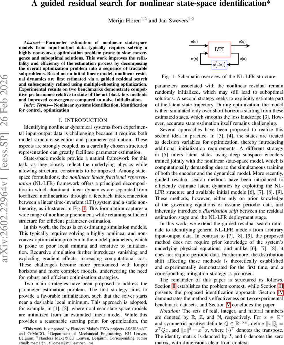
This paper tackles the notoriously difficult problem of identifying nonlinear state‑space models from input‑output data. The authors observe that direct estimation of such models leads to a highly non‑convex optimization problem, prone to poor local minima, slow convergence, and gradient issues (vanishing or exploding) when the model is simulated recursively over long horizons. To mitigate these challenges, they adopt the nonlinear linear fractional representation (NL‑LFR) framework, which cleanly separates dominant linear dynamics from localized static nonlinearities via a feedback interconnection.

The proposed identification strategy proceeds in three sequential stages.

1. Guided Residual Search – Starting from a stable linear model (the “best linear approximation”), the method estimates the matrices that couple the nonlinear residual (B_w, D_yw) and infers the latent residual signal w as well as the state trajectory x. This is formulated as a bilevel optimization: the inner level solves a sliding‑window least‑squares problem (window length H ≪ N) to obtain w and x given current coupling parameters; the outer level updates the coupling parameters by minimizing the output error over the whole data set. Closed‑form solutions are derived using the extended observability matrix and Toeplitz matrices, and a state‑normalization matrix T_x ensures unit‑variance scaling, improving numerical conditioning.
2. Nonlinear Residual Learning – The latent pairs (w*, x*) obtained from the first stage are treated as i.i.d. samples. A static nonlinearity f_NN is modeled by a feed‑forward neural network (with Xavier‑initialized weights) together with linear output matrices C_z and D_zu. The network is trained by minimizing the mean‑square error between the inferred residual w* and the network output ˆw* = f_NN(C_z x* + D_zu u). Because the samples are assumed independent, the training can be fully parallelized on a GPU, yielding fast convergence.
3. Multiple‑Shooting Final Optimization – The authors prove (Theorem 1) that when the nonlinear residual is learned in a decoupled fashion, one‑step prediction errors ε can grow exponentially during recursive simulation (‖x̂(N‑1) − x(N‑1)‖ ∈ O(L^{N‑1} ε) with Lipschitz constant L > 1). To prevent this distribution shift, they employ a multiple‑shooting scheme: the simulation horizon is split into short intervals of length d, each interval’s initial state is introduced as a decision variable, and continuity constraints enforce matching at interval boundaries. This reduces error accumulation, smooths the loss landscape, and enables the optimizer (IPOPT) to recover from non‑contractive regions. The initial values for both parameters and shooting states are taken directly from the guided residual search and neural‑network training, ensuring a well‑informed start.

Experimental validation is performed on two benchmark datasets: the Silverbox (an electronic mass‑spring‑damper with cubic stiffness) and a ground‑vibration test of an F‑16 aircraft. Both datasets are periodic, but the authors deliberately avoid exploiting periodicity beyond the initial linear model estimation. Implementations use Python, JAX/Optax for the first two stages, and CasADi/IPOPT for multiple shooting. Results show that the proposed method achieves root‑mean‑square errors comparable to or better than state‑of‑the‑art black‑box approaches, while requiring fewer iterations to converge. The guided residual search provides a robust initialization, and the multiple‑shooting refinement eliminates the exponential error growth predicted by the theory.

Key contributions of the paper are:

• A structured NL‑LFR formulation that separates linear and nonlinear components, making the identification problem more tractable.
• A bilevel guided residual search that efficiently infers latent residual dynamics and coupling matrices using closed‑form solutions within a sliding window.
• A theoretical analysis of distribution shift caused by decoupled residual training, quantified by a Lipschitz‑based error bound.
• The integration of multiple‑shooting to counteract error accumulation, leading to improved convergence and robustness.
• Empirical evidence on realistic benchmarks confirming competitive accuracy and faster convergence relative to existing methods.

Future work suggested includes automatic selection of window length H and shooting interval d, extension to multi‑input‑multi‑output (MIMO) systems, online/real‑time identification, and handling of non‑periodic or highly noisy data. Overall, the paper presents a compelling, theoretically grounded, and practically effective pipeline for nonlinear state‑space system identification.