Detection, coverage and percolation in dynamic Boolean models with random radii based on $α$-stable processes

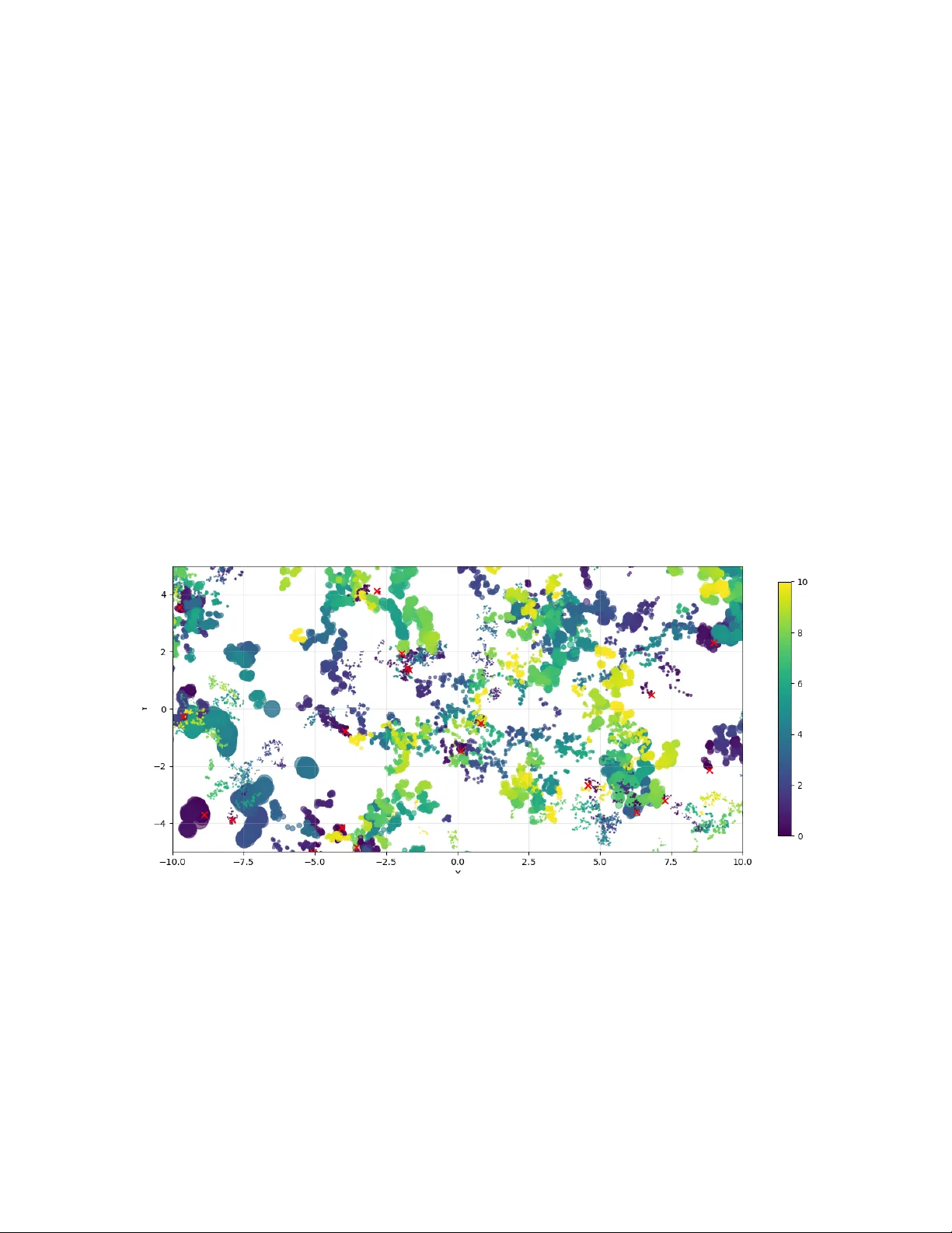
Detection, co vera ge and per cola tion in d ynamic Boolean models with random radi i based on α -st able pr ocesses P eter Gracar ∗ 1 , Benedikt Jahnel † 2,3 , Lukas Lüc h trath ‡ 3 , and Anh Duc V u § 3 1 Sc ho ol of Mathematics, Univ ersity of Leeds, Leeds LS2 9JT, UK 2 T ec hnische Universität Braunsch w eig, Braunsch w eig, Germany 3 W eierstrass Institute for Applied Analysis and Sto chastics, Berlin, German y F ebruary 26, 2026 Abstract W e consider a dynamic net work in con tin uum time and space in whic h no des, with initial lo- cations given by a Poisson p oint pro cess, mov e according to i.i.d. isotropic α -stable pro cesses. Eac h node is additionally equipped with an i.i.d. detection radius. Inspired by corresp onding results b y P eres et. al. on mobile net w orks based on Brownian sausages with ﬁxed width, w e in vestigate the tail b ehaviour of three stopping times: The detection time of the ﬁrst discov ery of a designated no de, the ﬁrst cov erage of an entire set, and the ﬁrst discov ery of a no de by the inﬁnite connected comp onent of the system. Broadly speaking, we disco ver that the sta- bilit y index as well as the random radii manifest themselv es only in constants in the otherwise exp onen tial deca y rates. The proofs rest on heat-k ernel bounds for the underlying Lévy pro- cesses and a detailed multiscale analysis allowing us to control the space-time correlations of the sy stem. AMS-MSC 2020 : Primary: 60D05; Secondary: 60K35 Keyw ords : mobile geometric graph, dynamic Bo olean mo del, p ercolation time, detection time, cov er- age time, Lévy process, α -stable pro cess, jump pro cess, Poisson p oin t pro cess, multiscale analysis ∗ Email: p.gracar@leeds.ac.uk; https://orcid.org/0000- 0001- 8340- 8340 † Email: b enedikt.jahnel@tu-braunsch weig.de; https://orcid.org/0000- 0002- 4212- 0065 ‡ Email: lukas.lue c htrath@wias-berlin.de; https://orcid.org/0000- 0003- 4969- 806X § Email: anhduc.vu@wias-b erlin.de; https://orcid.org/0009- 0005- 6913- 4992 1 1 In tro duction Mobile geometric graphs are fundamental mo dels for dynamic spatial net works, in which no des are distributed in space and form edges with nearby no des while moving according to some sto chastic dynamics [ 3 , 8 , 36 ]. Understanding ho w mobility and connectivity interact is crucial in many appli- cations, including wireless sensor netw orks, opinion dynamics, and epidemiology , see for example [ 1 , 10 , 15 , 16 , 17 , 20 , 23 ]. A rigorous mathematical framework is introduced in [ 27 ], where no des are initially placed according to a homogeneous Poisson p oint pro cess in R d and mov e independently according to Br ownian motions . No des are connected if their Euclidean distance is less than a ﬁxed radius r > 0 . They studied three fundamen tal quan tities: dete ction time , the ﬁrst moment when a target (ﬁxed or mobile) is within range of some node; c over age time , the time until a ﬁnite region has b een fully explored by the no des; and p er c olation time , the time un til a typical no de b ecomes part of the inﬁnite connected comp onent. Using sto chastic geometry , multiscale coupling, and concentration tec hniques, they deriv e dimension-dep enden t asymptotics for the upp er-tail probabilities of these times for a static or dynamic typical net work participant. In parallel, netw orks based on L évy jump pr o c esses , or Lévy ﬂights, hav e attracted attention due to their hea vy-tailed displacement distributions and scale-inv ariance prop erties, which provide goo d ﬁts to a large v ariet y of b eha viours observed in nature and engineering [ 11 , 13 , 32 , 35 ]. In this work, we com bine these strands by considering a dynamic geometric netw ork, in whic h no des follo w Lévy jump pro cesses rather than Bro wnian motions and radii are i.i.d. r andom variables in- stead of b eing globally ﬁxed. This setting captures b oth heavy-tailed mobilit y and heterogeneous in teraction ranges, which are common in real-w orld netw orks suc h as wireless communication sys- tems and animal mo v ement net works. By extending m ultiscale coupling and stochastic-geometric tec hniques to this ric her model, we characterise the asymptotic b ehaviour of detection, cov erage, and percolation times, generalising the ﬁndings in [ 27 ] to a more realistic non-Gaussian and het- erogeneous setting. The man uscript is organised as follows. In Section 2 w e ﬁrst present the setting and some basic prop erties of the underlying pro cesses that w e will frequently make use of. Then, we exhibit our main ﬁndings on the detection, cov erage, and p ercolation times including some case studies and pro vide an outlo ok for p ossible future research directions. The pro ofs are presented in Section 3 . 2 Setting and main results Fix the dimension d ≥ 1 , an intensit y λ > 0 and a stability index α ∈ (0 , 2] . A t time t = 0 , the no de locations Ψ 0 = { Ψ i } i ∈ N form a homogeneous Poisson p oint pr o c ess of intensit y λ on R d . W e equip each no de Ψ i , i ∈ N , with an i.i.d. copy R i of a c ommunic ation r adius R that satisﬁes 0 < E R d < ∞ . (1) Next, let X = ( X t ) t ≥ 0 b e the standar d d -dimensional isotr opic α -stable pr o c ess started in the origin o ∈ R d . That is, the L évy pr o c ess with c haracteristic function given b y the α -stable la w E exp(i ⟨ ξ , X t ⟩ ) = exp( − t | ξ | α ) , ∀ ξ ∈ R d , 2 with stability index α ∈ (0 , 2] . Recall that, as a Lévy pro cess, it has stationary , indep endent incremen ts and càdlàg paths and obeys the self-similarity (scaling) relation ( X ct ) t ≥ 0 d = ( c 1 /α X t ) t ≥ 0 , ∀ c > 0 . (2) Consequen tly , for α < 2 , each marginal X t has p olynomial tails, P ( | X t | > x ) ∼ C α tx − α , as x → ∞ for some C α > 0 , so in particular V ar | X t | = ∞ and, in case α ≤ 1 , even E | X t | = ∞ . The generator of the isotropic α -stable process is the fractional Laplacian − ( − ∆) α/ 2 so that the α = 2 case corresp onds to a standard Bro wnian motion at t wice the sp eed. W e now equip the no des of the Poisson p oint pro cess Ψ 0 with i.i.d. copies { Y i } i ∈ N of X and deﬁne X i := Y i + Ψ i . That is, eac h node of Ψ 0 mo ves indep endently according to a standard α -stable pro cess. W e denote the collection of all locations at time t by Ψ t = { X i t } i ∈ N . Thus, Ψ t has the la w of a homogeneous P oisson p oin t process with λ > 0 . Note that the asso ciated communication radii do not c hange ov er time. The main ob ject of in vestigation is the dynamic Bo ole an mo del G = ( G t ) t ≥ 0 , given by G t := [ i ≥ 1 B R i ( X i t ) ⊂ R d , t ≥ 0 , where B r ( x ) denotes the ball with radius r ≥ 0 cen tred at x ∈ R d , see Figure 1 for an illustration. The moment bound on the radius guarantees that this mo del is nontrivial, i.e. G t  = R d at each p oin t in time t ≥ 0 , see [ 3 , 24 ]. Figure 1: A realisation of the dynamic Bo olean mo del G based on the standard isotropic α -stable pro cess with α = 1 . 5 . Colour indicates time. As a Boolean mo del of a stationary Poisson p oin t pro cess, G t has the same distribution as G 0 for any t ≥ 0 . Plotted is ( G t ) t ∈ [0 , 10] . The starting conﬁguration is depicted by red crosses. 3 2.1 Detection times Our ﬁrst main result is concerned with the tail-b ehaviour of the ﬁrst time that the dynamic Bo olean mo del detects a target particle that is initially placed at the origin o ∈ R d . More precisely , we are in terested in the dete ction time , deﬁned as T g det := inf  t ≥ 0 : g ( t ) ∈ G t  = inf  t ≥ 0 : | g ( t ) − X i t | ≤ R i for some i ≥ 1  , (3) where g : [0 , ∞ ) → R d with g (0) = o is some measurable function that represents the mo vemen t of the no de that is to b e detected. In order to describe the exponential rate of decay of the tail probability of T g det , consider Γ t ⊂ R d , the tr aje ctory of the Lévy pro cess X up to time t and shifted by g , that is, Γ g t := [ s ≤ t { X s + g ( s ) } , where w e set Γ t := Γ o t . F urthermore, consider r -annuli around Lebesgue-measurable sets A ⊂ R d , deﬁned as B r ( A ) :=  x ∈ R d : | x − a | < r for some a ∈ A  , writing | A | for the d -dimensional Lebesgue-volume of A ⊂ R d . The probabilistic tail of the detection time can b e expressed in terms of the v olume of the Lévy sausage up to time t , for which w e refer to the following asymptotics, cf. [ 12 , Theorem 1 & 2], lim t ↑∞ 1 t E | B r (Γ t ) | = r d − α Cap( α, d ) , r ≥ 0 , (4) where Cap( α, d ) := 2 α π d/ 2 Γ( α/ 2) / Γ(( d − α ) / 2) with Γ( · ) b eing the gamma function. Moreov er, the function t 7→ E | B r (Γ t ) | − tr d − α Cap( α, d ) is monotonically increasing. The following ﬁrst result features the asymptotics of the upp er tails for the distribution of the detection time. W e highligh t that randomising the initial radii do es not c hange the asymptotic b eha viour in a qualitative wa y . This mainly follows from the fact that the volume asymptotics in ( 4 ) are con tin uous in the radius. Theorem 2.1 (Detection time) . Consider the dynamic Bo ole an mo del with α ∈ (0 , 2] and d > α . (i) If g ≡ o , then P ( T o det > t ) = exp  − tλ Cap( α, d ) E R d − α (1 + o (1))  , as t → ∞ and o (1) ≥ 0 . (ii) Ther e exists C ∈ (0 , 1] dep ending only on α and d such that for every me asur able g P ( T g det > t ) ≤ exp  − C tλ Cap( α, d ) E R d − α  , for al l t ≥ 0 . 4 (iii) If g is the r e alisation of an indep endent L évy pr o c ess Y , then for the anne ale d pr ob ability, lim t ↑∞ 1 t log P  T Y det > t  = sup t ≥ 1 1 t log P  T Y det > t  ∈ ( −∞ , 0) , i.e., a non-trivial exp onential r ate exists. (iv) If g β ( t ) := β tψ for some ψ ∈ R d \{ o } and β > 0 , then lim β ↑∞ lim t ↑∞ 1 t log P ( T g β det > t ) = −∞ , me aning that a very fast p article is dete cte d fast. Remark 2.2. Due to a r e arr angement ine quality [ 9 , The or em 1.5 & Cor ol lary 1.7], the statement in Part ( ii ) holds for C = 1 in the c ase wher e g is such that, for al l s ≥ 0 , ther e exists δ > 0 such that sup s ≤ t t ) = exp( − λ E | B R (Γ g t ) + K | ) . 2.2 Co v erage time Instead of detecting a single p oten tially moving particle, we now consider a static volume A ⊂ R d and ask ho w long it takes for the pro cess to hav e “seen” all of A . Put precisely , we are in terested in T cov ( A ) := inf n t ≥ 0 : A ⊂ [ s ≤ t G s o . While this question is diﬃcult to answer for individual A , we can give asymptotics on T cov ( k A ) for large k in terms of its Mink owski dimension β > 0 , that is, β := lim ε ↓ 0 log M ( A, ε ) / log( ε − 1 ) , if the limit exists and where M ( A, ε ) is the minimal num b er of balls of radius ε needed to co v er A . W e hav e the follo wing result, prov ed in Section 3.3 . Theorem 2.4 (Cov erage time) . Consider the dynamic Bo ole an mo del with α ∈ (0 , 2] and d > α . Then, for A ⊂ R d with Minkowski dimension β , lim k ↑∞ E T cov ( k A ) log( k ) = β λ Cap( α, d ) E R d − α . 5 2.3 P ercolation time Finally , we consider the p er c olation time of a target initially lo cated at the origin and that ma y or ma y not mov e. While the detection time deals with the question when the target is detected for the ﬁrst time b y any no de, the p ercolation time requires additionally that the detecting no de b elongs to the unb ounde d c omp onent at the time of detection. Recall that for d ≥ 2 there exists a critical intensit y λ c suc h that for all λ > λ c , the set G 0 con tains an unique un b ounded connected comp onent almost surely . As mentioned ab ov e, b y the displacement theorem for Poisson p oin t processes, at eac h time t , the set of no de locations Ψ t := { X i t } i ≥ 1 has the same distribution as Ψ 0 so that each Ψ t con tains such a comp onen t almost surely , and we write Ψ ∞ t ⊂ Ψ t for the set of all nodes that b elong to the un b ounded comp onent, and write G ∞ t := [ X i t ∈ Ψ ∞ t B R i ( X i t ) for the comp onen t itself. The p ercolation time is then deﬁned as T g perc := inf  t ≥ 0 : ∃ X i t ∈ Ψ ∞ t suc h that | X i t − g ( t ) | < R i  = inf  t ≥ 0 : g ( t ) ∈ G ∞ t  , where the function g : [0 , ∞ ) → R d , g (0) = o , describes the mov ement of the target. The next result giv es upp er tail-bounds for the detection time of a target that do es not mo ve to o quickly; particularly including the case where the origin do es not mov e at all. F or tw o functions f ≥ 0 and h > 0 , w e recall the Landau notation f = ω ( h ) for lim inf t →∞ f ( t ) /h ( t ) = ∞ and the notation f = o ( h ) for lim sup t →∞ f ( t ) /h ( t ) = 0 . Theorem 2.5 (P ercolation time) . Consider the dynamic Bo ole an mo del with α ∈ (0 , 2) and d ≥ 2 . F or any λ > λ c and function f ( t ) = ω (1) , ther e exists a c onstant c = c ( d, λ, α, f ) > 0 such that for al l g with | g ( t ) | = exp( o ( t/f ( t )) , we have, for al l suﬃciently lar ge t , P ( T g perc ≥ t ) ≤ exp  − ct/f ( t )  . Remark 2.6. The pr o of of The or em 2.5 r elies on the de c oupling r esult in Pr op osition 3.13 that al lows to indep endently r esample the Poisson p oints in a lar ge b ox for a p ositive fr action of time steps, se e also Se ction 2.4 for a mor e detaile d description of the underlying heuristics. The de c ou- pling r esult itself dep ends on heat-kernel b ounds and r elate d r esults for the α -stable pr o c ess and is thus only formulate d for α < 2 , cf. Se ction 3.2.1 . However, the r esult c an b e extende d, m utatis m utandis , to the α = 2 c ase by applying the Gaussian he at-kernel b ounds inste ad. By doing so, The or em 2.5 extends to α = 2 and ther eby impr oves the analo gous r esult [ 27 , The or em 1.6] for the Br ownian mo del with ﬁxe d r adii in two ways: First, by applying to r andom r adii; se c ond, impr ov- ing the c orr e ction term in the exp onential tail fr om p oly-lo garithm to any arbitr arily-slow gr owing function f . 2.4 Discussion and outlo ok Regarding detection times, one ma y sp eculate that the β -dependent constant in the exp onential tail of the probabilit y in Theorem 2.1 Part ( iv ) is increasing in β . This means, at least for linear motions, that the detection b ecomes faster if the target particle mo v es faster. F urthermore, note 6 that detection times can b e seen as hard-core v ariants of tr apping pr oblems as considered in [ 9 ]. In this class of mo dels, the co vered v olume | B R (Γ g t ) | is replaced by a more general energy term. F urthermore, in view of p eer-to-p eer ad-hoc net works, it is in teresting to study the ﬁrst time a target particle is detected for an uninterrupted time interv al [ t, t + a ] , for a ≥ 0 , reﬂecting the requirement that any transmission takes a minimal amount of time. Also, we susp ect a qualitatively similar picture if, instead of considering the detection time by a single no de, w e study the ﬁrst time a target is detected b y at least k ≥ 2 nodes, ma ybe ev en simultaneously . Similar extensions can also be considered in view of the co verage time, e.g., a minimal time of (uninterrupted) cov erage or cov erage by m ultiple no des. Also, what can b e said ab out c haracteristics b ey ond the expected v alue, suc h as the v ariance or large deviations? The pro of for the p ercolation time is based on the following strategy . F or d ≥ 2 and a P oisson in tensity λ > λ c , for each time, a typical no de is part of the unbounded comp onen t with probability θ = θ ( λ ) > 0 . In view of the p ercolation time with g ≡ o ﬁxed, on an intuitiv e level, one may expect the following: At the detection time T det , the origin has b een detected b y a no de of the unbounded comp onen t with probabilit y θ . If this is the case, then T perc = T det , and if not, one restarts the pro cesses to chec k again if the origin has been detected after some time has passed. Assuming enough indep endence, the num b er of trials follo ws a geometric distribution, which ultimately leads to an exp onential tail of T perc thanks to Theorem 2.1 . Ho wev er, this ignores the fact that the mo del is p ositively correlated. Indeed, a failed ﬁrst trial increases the probabilit y of failing again as the un b ounded component is, in that case, probably farther aw a y from the origin than on av erage. In order to tackle this issue, w e establish a result that ensures that the mo del mixes fast enough so that it b ehav es like an indep enden t, slightly thinned copy of itself at most integer time steps. This w as ﬁrst shown for a system of Brownian motions with a deterministic radius in [ 27 ]. The price we pa y using this approach is a correction f in the tail estimate of the p ercolation time, which may b e remo v able, but only with the help of new proof ideas. In view of Remark 2.2 , stating that a large class of moving targets is detected not slow er than a static target, it seems reasonable to believe that this is also true for p ercolation times. The general idea w ould b e that a mo ving target should lead to faster decoupling due to additional spatial decorrelations. Indeed, one might conjecture that for a fast and linearly moving target g β , as in Theorem 2.1 P art ( iv ) , w e ha v e lim β ↑∞ lim t ↑∞ 1 t log P ( T g β perc > t ) = log (1 − θ ) . Ho wev er, proving this also requires substantial additional eﬀort, which w e lea ve for future w ork. W e also remark that the condition on the displacement of g in Theorem 2.5 ensures appropriately comparable time and space scales. Relev an t examples of target no des, such as static or indep endent copies of the underlying particle mo v ement, are cov ered by this condition. A further c haracteristic to b e studied is the isolation time , i.e., T g iso := inf  t ≥ 0 : g ( t ) ∈ G t  , as studied in [ 29 ] for the case of Bro wnian motion. W e anticipate an exp onential tail behaviour similarly as for transient Brownian motions. On a general level, one may w onder how the system b ehav es if, instead of Γ t , one would consider Lévy sausages based on a contin uously interpolated path of the Lévy pro cesses. More generally , other mobilit y schemes suc h as random wa ypoint models, linear motions or jump-diﬀusion pro cesses 7 p oten tially yield diﬀerent qualitative b ehaviours. Let us also men tion that recently detection times ha ve also been analysed in h yperb olic space [ 22 ], op ening the do or tow ards the inv estigation of further netw ork c haracteristics in this setting. Finally , w e note that the mobile net w ork based on Lévy sausages can serv e as a relev ant dynamic graph mo del on whic h further dynamic pro cesses can b e studied. As a prime example, we think of the con tact process, as already in v estigated in dynamic lattice settings, see for example [ 7 , 21 , 33 , 34 ]. W e conjecture that phase transitions similar to the ones shown in [ 2 , 21 ] can b e sho wn, but lea ve this for future w ork. 3 Pro ofs 3.1 Pro ofs for detection times W e start b y pro ving the k ey Lemma 2.3 , whic h describ es detection times as void probabilities. Pr o of of Lemma 2.3 . W e adapt the pro of given in [ 27 ]. Recall that Ψ 0 ⊂ R d denotes the P oisson p oin t pro cess of in tensity λ > 0 represen ting the initial no de lo cations. Let Ψ ⊂ Ψ 0 denote the set of no des that detect any p oint in the (moving) compact set K up to time t ≥ 0 . As each node mo ves and p ossesses a random detection range, indep enden tly of the others, Ψ is an independent P oisson thinning and thus an inhomogeneous Poisson point process whose in tensity measure has Leb esgue density given by ρ ( x ) := λ P  ∃ s ≤ t : K + g ( s ) ∩ B R ( X s + x )  = ∅  = λ P  ∃ s ≤ t : x ∈ B R ( K + g ( s ) − X s )  = λ P  x ∈ B R (Γ g t ) + K  , where w e ha v e also used that X s has the same distribution as − X s in the last equalit y . Th us, the probabilit y of b eing undetected up to time t is the void probability P ( T g det ( K ) > t ) = P (Ψ = ∅ ) = exp  − Z R d λ P  x ∈ B R (Γ g t ) + K  d x  = exp  − λ E | B R (Γ g t ) + K |  , concluding the pro of. F rom no w on, w e will mainly concern ourselves with volume estimates to derive statements about detection probabilities. The following lemma will b e helpful. W e giv e the pro of later in this section. Lemma 3.1 (V olume b ounds) . L et A ⊂ R d b e a set, then | B r ( A ) | ≤ r d | B 1 ( A ) | . Returning to v olume asymptotics, recall that the radius R has ﬁnite d -th momen t. Lemma 3.2 (V olume asymptotics for random radii) . W e have for al l t ≥ 0 E | B R (Γ t ) | ≥ t Cap( α, d ) E R d − α and lim t ↑∞ 1 t E | B R (Γ t ) | = Cap( α, d ) E R d − α . Pr o of. Let M > 0 . Then, b y dominated con v ergence with majorant E | B M (Γ t ) | and [ 12 , Theo- rem 1 & 2], lim t ↑∞ 1 t E | B R (Γ t ) | ≥ lim t ↑∞ 1 t E  E | B R (Γ t ) | 1 { R < M }  = Cap( α, d ) E  R d − α 1 { R < M }  . 8 Th us, with M ↑ ∞ , w e hav e lim t ↑∞ 1 t E | B R (Γ t ) | ≥ Cap( α, d ) E R d − α . On the other hand, with the same arguments together with Lemma 3.1 , we hav e lim t ↑∞ 1 t E | B R (Γ t ) | = lim t ↑∞ 1 t E  E | B R (Γ t ) | 1 { R < M }  + lim t ↑∞ 1 t E  E | B R (Γ t ) | 1 { R ≥ M }  ≤ lim t ↑∞ 1 t E  E | B R (Γ t ) | 1 { R < M }  + lim t ↑∞ 1 t E | B 1 (Γ t ) | E  R d 1 { R ≥ M }  = Cap( α, d ) E  R d − α 1 { R < M }  + Cap( α, d ) E  R d 1 { R ≥ M }  < ∞ . So again, as M ↑ ∞ , w e ha v e lim t ↑∞ 1 t E | B R (Γ t ) | ≤ Cap( α, d ) E R d − α . The ﬁrst statement follows from the monotonicit y statemen t b elow ( 4 ). Let us turn our attention to moving particles. W e ha ve the follo wing low er volume b ound. Lemma 3.3 (Univ ersal lo wer volume b ound for drifts) . Ther e exists C ∈ (0 , 1] dep ending only on α and d such that E | B R (Γ g t ) | ≥ C E | B R (Γ t ) | ≥ C t Cap( α, d ) E R d − α . In the case of Brownian motions α = 2 , [ 28 ] shows that C = 1 even for non-measurable g . As men tioned in Remark 2.2 , C = 1 is only known under mild assumptions on g for α -stable pro cesses. Pr o of. It suﬃces to c hec k the statement for ﬁxed deterministic R = r > 0 . First, w e write Z t y := Z t 0 1  X s + g ( s ) ∈ B r ( y )  d s and note that we hav e P  Z t y > 0  = P  ∃ s ≤ t : X s + g ( s ) ∈ B r ( y )  . Th us, w e hav e E   B r (Γ g t )   = Z R d P  Γ g t ∩ B r ( y )  = ∅  d y = Z R d P  ∃ s ≤ t : X s + g ( s ) ∈ B r ( y )  d y = Z R d P  Z t y > 0  d y . Note that for general random v ariables Y ≥ 0 with P ( Y > 0) > 0 , w e hav e P ( Y > 0) = E Y / E [ Y | Y > 0] . Let us estimate the denominator. Denote b y τ the ﬁrst hitting time of (the closure of) B r ( y ) for Γ g t . The conditioning Z y > 0 is thus equiv alen t to τ < t , which in turn implies X τ + g ( τ ) ∈ B r ( y ) . Let Y = { Y s } s ≥ 0 b e an independent copy of X . Then, E  Z t y | Z t y > 0  = E h Z t 0 1  X s + g ( s ) ∈ B r ( y )  d s    τ < t i = E h Z t 0 1  X s + τ + g ( s + τ ) ∈ B r ( y )  d s    τ < t i = E h Z t − τ 0 1  X s + τ + g ( s + τ ) ∈ B r ( y )  d s    τ < t i = E h Z t − τ 0 1  X s + τ − X τ + g ( s + τ ) − g ( τ ) + X τ + g ( τ ) ∈ B r ( y )  d s    τ < t i . 9 By the strong Marko v property , the right-hand side can b e upper b ounded by E h Z t − τ 0 1  Y s + g ( s + τ ) − g ( τ ) ∈ B 2 r ( o )  d s    τ < t i = E h Z t − τ 0 P  Y s + g ( s + τ ) − g ( τ ) ∈ B 2 r ( o )  d s    τ < t i ≤ E h Z t − τ 0 P  Y s ∈ B 2 r ( o )  d s    τ < t i ≤ E h Z ∞ 0 P  Y s ∈ B 2 r ( o )  d s    τ < t i = Z ∞ 0 P  Y s ∈ B 2 r ( o )  d s = r α Z ∞ 0 P  Y s ∈ B 2 ( o )  d s = r α C < ∞ , due to transience of the α -stable process and where we used ( 2 ) in the second-to-last equality . On the other hand, Z R d E Z t y d y = Z R d E h Z t 0 1  X s + g ( s ) ∈ B r ( y )  d s i d y = Z R d Z t 0 P  X s + g ( s ) ∈ B r ( y )  d s d y = Z R d Z t 0 Z B r ( o ) f s  z + y − g ( s )  d z d s d y = Z t 0 Z B r ( o ) 1d s d y = t | B r ( o ) | . Putting everything together, w e ha v e E | B r (Γ g t ) | ≥ r − α t | B r ( o ) | /C , which ﬁnishes the pro of. Pr o of of The or em 2.1 . Items (i) and (ii) are direct consequences of the Lemmas 3.2 and 3.3 after applying Lemma 2.3 . F or Item (iii) note that for all t, t ′ ≥ 0 w e ha v e that P  T Y det > t + t ′  = P  o / ∈ B R (Γ Y t + t ′ )  = E Y  exp( − λ E X | B R (Γ Y t + t ′ ) | )  = E Y h exp  − λ E X    [ s ≤ t + t ′ B R ( X s + Y s )    i ≥ E Y h exp  − λ E X h    [ s ≤ t B R ( X s + Y s )    +    [ t ≤ s ≤ t + t ′ B R ( X s + Y s )    ii = E Y h exp  − λ E X    [ s ≤ t B R ( X s + Y s )    i E Y h exp  − λ E X    [ s ≤ t ′ B R ( X s + Y s )    i = P  T Y det > t  P  T Y det > t ′  , where w e used indep endent increments and shift-in v ariance in space and time in the fourth line. Th us, − log P ( T Y det > t ) is subadditive, so lim t ↑∞ 1 t log P ( T Y det > t ) = sup t ≥ 1 1 t log P ( T Y det > t ) by F ek ete’s Lemma. It remains to sho w that this limit is nontrivial. Item (ii) giv es an upp er b ound of − C λ Cap( α, d ) E R d − α . With regards to the lo wer bound, it suﬃces to chec k P ( T Y det > 1) > 0 . Since Y is a Lévy pro cess and in particular càdlàg, there exists some M > 0 with P ( Y [0 , 1] ⊂ B M ( o )) =: ε > 0 . Consider the dynamic Bo olean model with the radii enlarged b y M , i.e., ˜ G t := ∪ i ≥ 1 B R i + M ( X i t ) = B M ( G t ) . Then, the detection time ˜ T o det for this model satisﬁes, by Item (i), P ( ˜ T o det > 1) = exp  − λ Cap( α, d ) E [ ( R + M ) d − α ](1 + o (1))  =: δ > 0 . 10 Since Y is independent of X i and R i , we hav e P  o / ∈ [ s ≤ 1 B M ( G s ) and Y [0 , 1] ⊂ B M ( o )  = P  ˜ T o det > 1 and Y [0 , 1] ⊂ B M ( o )  = εδ > 0 . Ho wev er, this ev ent implies { Y s / ∈ G s ∀ s ≤ 1 } = { T Y det > 1 } , pro ving the claim. F or Item (iv), it suﬃces to show that lim β ↑∞ lim t ↑∞ 1 t lim β ↑∞ E   S s ≤ t B R  X s − g β ( s )    = ∞ . In- sp ecting the proof of Lemma 3.3 , w e see that it suﬃces to show that lim β ↑∞ lim t ↑∞ sup y ∈ R d E  Z t,β y   Z t,β y > 0  = 0 . F or this, w e can follow the initial steps as ab o ve, and bound lim β ↑∞ lim t ↑∞ sup y ∈ R d E  Z t,β y   Z t,β y > 0  ≤ lim β ↑∞ Z ∞ 0 P  Y s − g β ( s ) ∈ B 2 R ( o )  d s = Z ∞ 0 lim β ↑∞ P  Y s ∈ B 2 R ( g β ( s ))  d s = Z ∞ 0 lim β ↑∞ P  s 1 /α Y 1 ∈ B 2 R ( g β ( s ))  d s = Z ∞ 0 lim β ↑∞ P  Y 1 ∈ B 2 R/s 1 /α ( β s 1 − 1 /α ψ )  d s = 0 , b y dominated con vergence with majorant 1 { s ≤ 1 } + P  Y s ∈ B 2 R ( o )  , which is integrable by tran- sience of the pro cess. In the last line w e again used ( 2 ). Let us ﬁnish the section with the proof of Lemma 3.1 . T o do so, we ﬁrst show tw o auxiliary results. Lemma 3.4. L et x ∈ R d , 0 ≤ r 1 ≤ r 2 and c ∈ [0 , 1] . Then, B r 1 ( o ) ∩ B r 2 ( x ) ⊂ B r 1 ( o ) ∩ B r 2 ( cx ) . (5) Pr o of. Let y ∈ B r 1 ( o ) ∩ B r 2 ( x ) . Then, ∥ y ∥ < r 1 and ∥ x − y ∥ < r 2 . By con v exity of the norm and r 1 ≤ r 2 , we hav e D ( c ) = ∥ cx − y ∥ ≤ c ∥ x − y ∥ + (1 − c ) ∥ y ∥ < cr 2 + (1 − c ) r 1 ≤ r 2 . Th us, y ∈ B r 2 ( cx ) , proving the claim. Lemma 3.5. L et A ⊂ R d b e a set and c ∈ [ 0 , 1] . Then, | B r ( A ) | ≥ | B r ( cA ) | . Pr o of. Let us ﬁrst consider the case where A consists of ﬁnitely man y p oints, i.e., we ha ve A = { x 0 , x 1 , . . . , x n } . W e prov e the claim by induction. The claim is trivial for singletons. After shifting, w e may , without loss of generality , assume x 0 = o . W rite A 1 = A \{ o } . Then, | B r ( cA 1 ) | ≤ | B r ( A 1 ) | . F urthermore, | B r ( A ) | = | B r ( o ) | + | B r ( A 1 ) | − | B r ( o ) ∩ B r ( A 1 ) | and 11 | B r ( cA ) | = | B r ( o ) | + | B r ( cA 1 ) | − | B r ( o ) ∩ B r ( cA 1 ) | . Th us, w e only need to show that B r ( o ) ∩ B r ( A 1 ) ⊂ B r ( o ) ∩ B r ( cA 1 ) . But this follo ws from ( 5 ) via B r ( o ) ∩ B r ( A 1 ) = n [ i =1 B r ( o ) ∩ B r ( x i ) ⊂ n [ i =1 B r ( o ) ∩ B r ( cx i ) = B r ( o ) ∩ B r ( cA 1 ) and so the claim holds true in the ﬁnite case. Let us mov e on to arbitrary A ⊂ R d . First, we ma y assume that A is b ounded, since otherwise | B r ( A ) | = | B r ( cA ) | = ∞ . Let ε > 0 . Then, w e ﬁnd a ﬁnite set I ( ε ) ⊂ A suc h that B r − ε ( A ) ⊂ B r ( I ( ε )) , since the closure of B r − ε ( A ) is compact and cov ered by { B r ( x ) } x ∈ A . W e sho w B r − ε ( cA ) ⊂ B r ( cI ( ε )) . This will yield the claim since B r ( cA ) ↖ ε ↓ 0 B r − ε ( cA ) ⊂ B r ( cI ( ε )) and B r ( I ( ε )) ⊂ B r ( A ) , as well as | B r ( cI ( ε )) | ≤ | B r ( I ( ε )) | since I ( ε ) is ﬁnite. Let a ∈ B r − ε ( cA ) . Hence, we ﬁnd some x ∈ A such that | a − cx | < r − ε . On the other hand, | a + (1 − c ) x − x | = | a − cx | < r − ε and th us a + (1 − c ) ∈ B r − ε ( A ) . Therefore, a + (1 − c ) x ∈ B r ( y ) for some y ∈ I ( ε ) . As suc h, we need to sho w a ∈ B r ( cy ) . Using ( 5 ), w e hav e a − cx ∈ B r − ε ( o ) ∩ B r ( y − x ) ⊂ B r − ε ( o ) ∩ B r ( cy − cx ) , whic h implies r > ∥ a − cx − cy + cy ∥ = ∥ a − cy ∥ , i.e., a ∈ B r ( cy ) . This ﬁnishes the pro of. Pr o of of Lemma 3.1 . The claim follows from Lemma 3.5 , which yields | B 1 ( r − 1 A ) | ≤ | B 1 ( A ) | . Thus, | B r ( A ) | = | r · B 1 ( r − 1 A ) | = r d | B 1 ( r − 1 A ) | ≤ r d | B 1 ( A ) | , as desired. 3.2 Prerequisite results on α -stable pro cesses The isotropic α -stable process has the Lévy intensit y function (or jump activity) J ( x, y ) := C | x − y | − ( d + α ) , x, y ∈ R d , (6) for some C > 0 . 12 3.2.1 Heat-k ernel b ounds, parab olic Harnac k inequality and Hölder inequalit y The follo wing statement is an application of [ 5 , Theorem 1.2] to the sp eciﬁc case of isotropic α -stable pro cesses on R d . Theorem 3.6 (Heat-kernel bounds) . The tr ansition pr ob ability at time t ≥ 0 of an isotr opic α - stable pr o c ess on R d with α ∈ (0 , 2] has a L eb esgue density p ( t, · , · ) : R d × R d → [ 0 , 1] such that ther e exist c onstants c 1 , c 2 , C > 0 with C − 1  t − d/α ∧ c 1 t | x − y | d + α  ≤ p ( t, x, y ) ≤ C  t − d/α ∧ c 2 t | x − y | d + α  , for al l t > 0 , x, y ∈ R d . Pr o of. In the notation of [ 5 ], we choose V ( r ) = r d and ϕ ( r ) = r α . Consequen tly , with ρ b eing the Euclidean metric on F = R d , the jump activity satisﬁes Condition (1.9) from [ 5 ], i.e., J ( x, y ) ≍ 1 V ( ρ ( x, y )) ϕ ( ρ ( x, y )) . Then, [ 5 , Condition (1.1)] is satisﬁed for the Euclidean metric on R d , as is Condition (1.8) that µ ( B ( x, r )) ≍ V ( r ) for x ∈ R d and r > 0 (here, µ is the Leb esgue measure on R d ). Condition (1.11) is also trivially satisﬁed for V ( r ) = r d . In our case, ϕ ( r ) = r α , so ϕ 1 ( r ) = r α and ψ ( r ) = 1 , so in the notation of [ 5 ], Condition (1.12) is satisﬁed with γ 1 = γ 2 = 0 and b y [ 5 , Theorem 1.2], the heat-k ernel bounds obtained hold for all t > 0 and all x, y ∈ R d . W e sa y that a non-negativ e Borel measurable function h ( t, x ) on [0 , ∞ ) × R d is p ar ab olic in a relativ ely open subset D of [0 , ∞ ) × R d if, for ev ery relativ ely compact open subset D 1 of D , h ( t, x ) = E ( t,x ) [ h ( Z τ D 1 )] for every ( t, x ) ∈ D 1 , where Z s = ( V s , X s ) is the space-time process with V s = V 0 + s for some V 0 ∈ R and τ D 1 = inf { s > 0 : Z s ∈ D 1 } . Note in particular that the transition densit y of the isotropic α -stable pro cess p ( t, x, y ) is parab olic as a function of t and y . F or each r, t > 0 , x ∈ R d and γ ∈ (0 , 1 / 2) deﬁne the cylinder Q ( t, x, r ) := [ t, t + γ r α ] × B r ( x ) . Theorem 3.7 (Parabolic Harnac k inequality) . Consider the he at kernel p as b efor e. Then, ther e exists c 1 > 0 such that for every z ∈ R d , r > 0 and every non-ne gative function h on [ 0 , ∞ ) × R d that is p ar ab olic and b ounde d on Q (0 , x, 2 r ) , we have sup ( t,y ) ∈ Q ( r α ,z ,r ) h ( t, y ) ≤ c 1 inf y ∈ B r ( z ) h (0 , y ) . In p articular, for t > 0 , sup ( s,y ) ∈ Q ((1 − γ ) t,z ,t 1 /α ) p ( s, x, y ) ≤ c inf y ∈ B t 1 /α ( z ) p ((1 + γ ) t, x, y ) . Pr o of. The statemen t is [ 5 , Theorem 4.12] applied to our setting of isotropic α -stable pro cesses (as depicted in the pro of of Theorem 3.6 with δ = 1 ). F or our purposes, the key consequence of the parab olic Harnack inequality is that the heat kernel of an isotropic α -stable pro cess is Hölder con tin uous. 13 Prop osition 3.8 (Hölder contin uity) . F or every r 0 > 0 ther e exist c onstants c, κ > 0 such that for every 0 < r < r 0 and every b ounde d p ar ab olic function h on Q (0 , x 0 , 2 r ) , | h ( s, x ) − h ( t, y ) | ≤ c ∥ h ∥ ∞ , R d r − κ ( | t − s | 1 /α + | x − y | ) κ holds for ( s, x ) , ( t, y ) ∈ Q (0 , x 0 , r ) , wher e ∥ h ∥ ∞ , R d := sup ( t,y ) ∈ [0 ,γ (2 r ) α ] × R d | h ( t, y ) | . In p articular, for p and any T > 0 and t 0 ∈ (0 , T ) , ther e exist c onstants c > 0 and κ > 0 such that for any t, s ∈ [ t 0 , T ] and x i , y i ∈ R d × R d with i = 1 , 2 , | p ( s, x 1 , y 1 ) − p ( t, x 2 , y 2 ) | ≤ ct − ( d + κ ) /α 0 ( | t − s | 1 /α + | x 1 − x 2 | + | y 1 − y 2 | ) κ . Pr o of. Again, this statemen t is [ 5 , Proposition 4.14] applied to our setting of isotropic α -stable pro cesses (as depicted in the pro of of Theorem 3.6 ). 3.2.2 Escape and hitting probabilities W e will need b ounds on the probabilities of either escaping some ball of radius r or hitting some far-a wa y ball of radius r . Prop osition 3.9 (Escap e probability) . L et τ r := inf { t > 0 : | X t | ≥ r } b e the ﬁrst time the isotr opic α -stable pr o c ess with α < 2 is at le ast r away fr om its starting lo c ation o . Then, ther e exists C > 0 such that P ( τ r ≤ t ) ≤ C r − α t, for al l r > 0 , t < r α . Pr o of. W e ﬁrst c heck that its jump activit y J satisﬁes Z | z | 2 1 + | z | 2 J ( o, z )d z < ∞ for every α < 2 . Our process starts in the origin b y assumption, so [ 31 , Equation (3.2)] gives for ev ery t > 0 , r > 0 , P ( τ r ≤ t ) = P  sup s ≤ t | X s | ≥ r  ≤ c 2 min { 1 , th ( r ) } , where h ( r ) = K ( r ) + L ( r ) with K ( r ) = R | z |≤ r r − 2 | z | 2 J ( o, z )d z and L ( r ) = R | z | >r J ( o, z )d z (the third term in [ 31 ] v anishes due to rotational inv ariance). Th us, the isotropic α -stable pro cess giv es h ( r ) ≍ r − α . Hence, there exists C > 0 suc h that, uniformly for arbitrary t satisfying t ≤ r α , P ( τ r ≤ t ) ≤ C r − α t, as desired. The following result estimates how far the α -stable pro cess X can trav el without large jumps. F or this, we decomp ose X into indep enden t pro cesses X = X ′ + X ′′ , 14 where X ′ has jump activity J ( x, y ) 1 {| x − y | ≥ 1 } and X ′′ has jump activity J ( x, y ) 1 {| x − y | < 1 } . Th us, X ′ is a c omp ound Poisson pr o c ess of ﬁnite activity R B 1 ( o ) ∁ J ( o, x )d x ∈ (0 , ∞ ) only consisting of jumps of size ≥ 1 . On the other hand, X ′′ is a pure-jump martingale having only jumps of size less than 1 , i.e., it is the truncated α -stable process. Lemma 3.10 (Escap e probability of truncated pro cess) . L et r ≥ 0 b e ﬁxe d and α ∈ (0 , 2) . Then, ther e ar e c onstants C , C ′ , κ > 0 , such that P  max s ≤ t | X ′′ s | ≥ L  ≤ C exp  − κ ( L − C ′ t )  , for al l L ≥ 0 , t ≥ 1 . Pr o of. Denote the heat kernel of X ′′ b y p − ( t, y , x ) . By [ 4 , Theorem 2.3], there exist C ∗ , c 1 , c 2 > 0 suc h that for ev ery | x | ≥ C ∗ t , we hav e p − ( t, o, x ) ≤ c 1 exp  − c 2 | x | log ( | x | /t )  ≤ c 1 exp  − 2 κ | x |  , where κ := 1 2 c 3 log C ∗ . On the other hand, we also hav e for every t ≥ 1 and every x ∈ R d b y [ 4 , Prop osition 2.2] that p − ( t, o, x ) ≤ c 1 t − d/ 2 . W e use Doob’s martingale inequalit y to b ound for all κ > 0 P  max s ≤ t | X ′′ s | ≥ ℓ  ≤ exp( − κℓ ) E exp( κ | X ′′ t | ) . Th us, with constants C > 0 only depending on d, C ∗ , κ c hanging from line to line E exp( κ | X ′′ t | ) = Z R d p − ( t, o, x ) exp( κ | x | )d x ≤ Z | x |≤ C ∗ t c 1 t − d/ 2 exp( κ | x | )d x + Z | x |≥ C ∗ t c 1 exp( − 2 κ | x | ) exp( κ | x | )d x ≤ C t − d/ 2 Z C ∗ t 0 z d − 1 exp( κz )d z + C Z ∞ 0 z d − 1 exp( − κz )d z ≤ C t d/ 2 − 1 exp( κC ∗ t ) + C ≤ C exp(2 κC ∗ t ) . Therefore, we conclude P  max s ≤ t | X ′′ s | ≥ L  ≤ exp( − κL ) E exp( κ | X ′′ t | ) ≤ C t d/ 2 − 1 exp  − κ ( L − 2 C ∗ t )  , as desired. Lemma 3.11 (Hitting probability of far-aw a y sets) . Ther e exist C , C ′ , κ > 0 (only dep ending on d and α ) such that for every t ≥ 1 , x ∈ R d and r, L > 0 with r + L ≤ | x | / 6 , we have P  ∃ s ≤ t : X s ∈ B r ( x )  ≤ C  | x | − ( d + α ) t 2 ( r + L ) d + exp  − κ ( L/ 2 − C ′ t )   . In p articular, by cho osing L := t log | x | and if | x | ≥ t , we have asymptotic al ly as t ↑ ∞ that P  ∃ s ≤ t : X s ∈ B r ( x )  ≤ C | x | − d − α + o (1) t 2+ d . 15 Pr o of. First, we note that  ∃ s ≤ t : X s ∈ B r ( x )  ⊂ n max s ≤ t | X ′′ s | ≥ L/ 2 o ∪  X has a jump of size ≥ 1 in to B r + L ( x ) b efore time t  . This is due to the fact that if X s hits B r ( x ) without ha ving a jump of size at least ≥ 1 into B r + L ( x ) , then X had to mov e from R d \ B r + L ( x ) to B r ( x ) without any jumps of size ≥ 1 . This implies that the truncated process X ′′ has tw o p oints of distance at least L to eac h other up to time t , which sho ws the set inclusion of the even ts. The probabilit y of the ﬁrst even t can be estimated using the previous lemma, yielding P  max s ≤ t | X ′′ s | ≥ L/ 2  ≤ C exp  − κ ( L/ 2 − C ′ t )  . F or the probabilit y of the second ev ent, we use sev eral steps. First, note that X having a jump of size ≥ 1 is the same as X ′ p erforming such a jump. The result will follo w from the Marko v inequalit y and Marko v prop erty of the jump process as follows. Let us split the even t { X has a jump of size ≥ 1 in to B r + L ( x ) } in to the cases where the jump has size ≥ | x | / 3 or not. If the jump has size ≥ | x | / 3 , then with constan ts C c hanging from line to line (indep enden t of t, L, x, r but not d, α ), P  X has jump of size ≥ | x | / 3 in to B r + L ( x )  ≤ E  # { jumps of size ≥ | x | / 3 in to B r + L ( x ) }  = Z t 0 Z R d E  # { jumps of size ≥ | x | / 3 in to B r + L ( x ) } from y at time s  d y d s = Z t 0 Z R d p ( s, o, y ) Z R d 1 { y + z ∈ B r + L ( x ) } 1 {| z | ≥ | x | / 3 }J ( y , y + z ) 1 {| z | ≥ 1 } d z d y d s ≤ C Z t 0 Z R d p ( s, o, y ) Z R d 1 { y + z ∈ B r + L ( x ) } 1 {| z | ≥ | x | / 3] }| z | − ( d + α ) d z d y d s ≤ C | B r + L ( o ) | ( | x | / 3) − ( d + α ) Z t 0 Z R d p ( s, o, y )d y d s ≤ C ( r + L ) d | x | − ( d + α ) t. On the other hand, if the jump has size ∈ [1 , | x | / 3] , then X had to b e in B | x | / 3+ r + L ( x ) ⊂ B | x | / 2 ( x ) prior to the jump. In particular, this has distance ≥ | x | / 2 to the origin. By the assumption r + L ≤ | x | / 6 , we get | x | / 2 ≥ | x | / 3 + r + L . Thus, using the heat-kernel estimates on X , Theorem 3.6 , as well as the ﬁnite jump rate of X ′ , we hav e with constan ts C c hanging from line to line P  X has jump of size ∈ [1 , | x | / 3] into B r + L ( x )  ≤ E  # { jumps of size ∈ [1 , | x | / 3] into B r + L ( x ) }  = Z t 0 Z R d p ( s, o, y ) ν Z R d 1 { y + z ∈ B r + L ( x ) } 1 { 1 ≤ | z | ≤ | x | / 3 }J ( y , y + z ) 1 {| z | ≥ 1 } d z d y d s = Z R d 1 { 1 ≤ | z | ≤ | x | / 3 }J ( o, z )d z Z t 0 Z B | x | / 2 ( x ) ∩ B r + L ( z − x ) p ( s, o, y )d y d s ≤ C Z t 0 Z B | x | / 2 ( x ) ∩ B r + L ( z − x ) s | y | d + α d y d s 16 ≤ C Z t 0 Z B | x | / 2 ( x ) ∩ B r + L ( z − x ) t ( | x | / 2) d + α d y d s ≤ C t 2 | B r + L ( o ) || x | − ( d + α ) ≤ C ( r + L ) d | x | − ( d + α ) t 2 , with C only dep ending on d and α as b efore, whic h ﬁnishes the proof. 3.3 Pro ofs for co v erage times Pr o of of The or em 2.4 (upp er b ound). A simple rescaling sho ws that M ( kA, ε ) = M ( A, ε/k ) . Let us ﬁx ε, δ > 0 . By the deﬁnition of β , w e hav e for suﬃciently large k ( ε − 1 k ) α + δ ≥ M ( A, ε/k ) . Th us, we can cov er k A if w e detect all the M ( kA, ε ) man y centres of the ε -balls using balls of radius R − ε . Let us write I ( ε ) := E  ( R − ε ) d − α 1 { R ≥ ε }  and note that I ( ε ) → I (0) = E R d − α as ε ↓ 0 . By Lemmas 2.3 and 3.2 P  T cov ( k A ) > t  ≤ P ( some cen tre is not co vered up to time t using smaller radii ) ≤ M ( A, ε/k ) P ( o is not cov ered using radii R − ε ) ≤ M ( A, ε/k ) exp  − λ E | B R − ε Γ t |  ≤ M ( A, ε/k ) exp  − λt Cap( α, d ) I ( ε )  . Th us, for any t ∗ ≥ 0 , w e ha v e E T cov ( k A ) = Z ∞ 0 P  T cov ( k A ) > t  d t ≤ t ∗ + Z ∞ t ∗ M ( A, ε/k ) exp  − λt Cap( α, d ) I ( ε )  d t. W e wan t to c ho ose t ∗ := t ∗ ( k ) such that 1 = ( ε − 1 k ) β +2 δ exp  − λt ∗ Cap( α, d ) I ( ε )  . (7) In particular, t ∗ ↑ ∞ as k ↑ ∞ and Z ∞ t ∗ M ( A, ε/k ) exp  − λt Cap( α, d ) I ( ε )  d t = t ∗ Z ∞ 1 M ( A, ε/k ) exp  − λ ( t ∗ t )Cap( α, d ) I ( ε )  d t = M ( A, ε/k ) ( ε − 1 k ) β +2 δ t ∗ Z ∞ 1 exp  − λt ∗ Cap( α, d ) I ( ε )  t − 1 d t = M ( A, ε/k ) ( ε − 1 k ) β +2 δ t ∗ λt ∗ Cap( α, d ) I ( ε ) ≤ ( ε − 1 k ) β + δ ( ε − 1 k ) β +2 δ 1 λ Cap( α, d ) I ( ε ) = ( ε − 1 k ) − δ λ Cap( α, d ) I ( ε ) k ↑∞ − − − → 0 , using ( 7 ) in the second step. Thus, we only need to estimate t ∗ ( k ) . F or this, we can bound t ∗ ( k ) ≤ ( β + 2 δ ) log( ε − 1 k ) λ Cap( α, d ) I ( ε ) = ( β + 2 δ ) log( k ) λ Cap( α, d ) I ( ε ) + c ( ε ) with c ( ε ) not dep ending on k . As δ > 0 w as arbitrarily chosen, we hav e that lim k ↑∞ E T cov ( k A ) log( k ) ≤ β λ Cap( α, d ) I ( ε ) . Finally , taking ε ↓ 0 pro v es the claim. 17 Regarding the low er b ound, we need an estimate for the hitting times of balls that are v ery far a wa y . In the case of α = 2 , i.e., Brownian motion, this follows from readily av ailable results, see for example [ 19 ]. Lemma 3.11 suﬃces for our purp ose. Pr o of of The or em 2.4 (lower b ound). W e use the alternative characterisation of the Minko wski di- mension, where A ⊂ R d has Minko wski dimension β > 0 if β = lim k ↑∞ log M ( k A ) / log( k ) , where still M ( k A ) is the maximal possible n umber of disjoint balls of radius 1 with centres in kA . By this deﬁnition of β , we ha ve for every δ > 0 that k β − δ ≤ M ( k A ) ≤ k β + δ , for all suﬃcien tly large k . Thus, w e know that ℓA is not cov ered if at least one of those M ( ℓA ) man y points is not detected. Let us denote the random v ariable U t := # { undetected p oints out of the M ( ℓA ) many up to time t ≥ 0 } . Clearly , P ( T cov > t ) ≥ P ( U t > 0) . Fix some small ε > 0 . Let us again consider a sp ecial time t ∗ := t ∗ ( k ) = β − δ − ε λ Cap( α, d ) E R d − α log k. Then, we see that E T cov ( k A ) = Z ∞ 0 P  T cov ( k A ) > t  d t ≥ Z t ∗ 0 P  T cov ( k A ) > t  d t ≥ t ∗ P  T cov ( k A ) > t ∗  . As suc h, the claim follo ws by sho wing P  T cov ( k A ) > t ∗  → 1 as k ↑ ∞ . By the second-moment metho d P  T cov ( k A ) > t ∗  = P ( U t ∗ > 0) ≥ E | U t ∗ | 2 / E | U 2 t ∗ | , where, by stationarity , E | U t ∗ | = M ( k A ) exp  − λ E | B R (Γ t ∗ ) |  . W e are looking for a suitable upp er b ound for the denominator. Let us denote the M ( k A ) many cen tres of the balls by x i . Then, using Lemma 2.3 for 2-p oin t sets, we ha ve E | U 2 t ∗ | = X i ≤ M ( kA ) X j ≤ M ( kA ) P ( x i , x j b oth undetected ) = E U t ∗ + X i ≤ M ( kA ) X i  = j exp  − λ E | B R (Γ t ∗ ) ∪ B R (Γ x j − x i t ∗ ) |  = E U t ∗ + X i ≤ M ( kA ) X i  = j exp  − 2 λ E | B R (Γ t ∗ ) |  exp  λ E | B R (Γ t ∗ ) ∩ B R (Γ x j − x i t ∗ ) |  . (8) Th us, we hav e to deal with M ( k A ) 2 man y summands and w ant to sho w E | B R (Γ t ∗ ) ∩ B R (Γ x j − x i t ∗ ) | → 0 in some w a y . First of all, w e may safely disregard o ( M ( k A ) 2 ) many pairs of vertices. Thus, we exclude all i, j which satisfy | x i − x j | < M ( k A ) 1 /d  log M ( k A ) =: L ( k ) . 18 No w, consider for a ﬁxed r ≥ 0 , F ( t, y, r ) := E   B r (Γ t ) ∩ B r (Γ y t )   = Z R d P  o Γ t ⇝ B r ( x ) and o Γ t ⇝ B r ( x − y )  d x, where o Γ t ⇝ B r ( X ) means that Γ t is a path from o in to B r ( x ) , and split the exp ected ov erlap into E   B R (Γ t ∗ ( k ) ) ∩ B R (Γ y t ∗ ( k ) )   = E  F ( t ∗ ( k ) , y , R ) 1 { R < L ( k ) α/ 2 d / 4 }  + E  F ( t ∗ ( k ) , y , R ) 1 { R ≥ L ( k ) α/ 2 d / 4 }  . (9) W e will show that each of those summands tends to 0 as k ↑ ∞ . Let us start with the second summand. Using ( 2 ) as well as Lemma 3.1 and noting that R ≥ L ( k ) α/ 2 d / 4 and L ( k ) α/ 2 d / 4 ≥ t ∗ ( k ) 1 /α for large enough k , w e get E  F ( t ∗ ( k ) , y , R ) 1 { R ≥ L ( k ) α/ 2 d / 4 }  ≤ E  E | B R (Γ t ∗ ( k ) ) | 1 { R ≥ L ( k ) α/ 2 d / 4 }  = E  t ∗ ( k ) d/α E | B Rt ∗ ( k ) − 1 /α (Γ 1 ) | 1 { R ≥ L ( k ) α/ 2 d / 4 }  ≤ E  R d E | B 1 (Γ 1 ) | 1 { R ≥ L ( k ) α/ 2 d / 4 }  = C E  R d 1 { R ≥ L ( k ) α/ 2 d / 4 }  k ↑∞ − − − → 0 , since E R d < ∞ . Regarding the ﬁrst summand in ( 9 ), w e ma y no w restrict ourselves to the case of R ≤ L ( k ) α/ 2 d / 4 , for whic h w e will deriv e uniform upper bounds. Using the Mark ov property , we can b ound P  o Γ t ⇝ B R ( x ) , o Γ t ⇝ B R ( x − y )  ≤ P  {∃ s ≤ s ′ ≤ t : X s ∈ B R ( x ) , X s ′ ∈ B R ( x − y ) } ∪ {∃ s ′ ≤ s ≤ t : X s ∈ B R ( x ) , X s ′ ∈ B R ( x − y ) }  ≤ P  ∃ s ≤ s ′ ≤ s + t : X s ∈ B R ( x ) , X s ′ ∈ B R ( x − y )  + P  ∃ s ′ ≤ s ≤ s ′ + t : X s ∈ B R ( x ) , X s ′ ∈ B R ( x − y )  ≤ P  ∃ s ≤ t : X s ∈ B R ( x )  P  ∃ s ′ ≤ t : Y s ′ ∈ B 2 R ( − y )  + P  ∃ s ≤ t : Y s ∈ B 2 R ( y )  P  ∃ s ′ ≤ t : X s ′ ∈ B R ( x − y )  ≤ P  ∃ s ≤ t : X s ∈ B 2 R ( x )  P  ∃ s ≤ t : X s ∈ B 2 R ( − y )  + P  ∃ s ≤ t : X s ∈ B 2 R ( y )  P  ∃ s ≤ t : X s ∈ B 2 R ( x − y )  = 2 P  ∃ s ≤ t : X s ∈ B 2 R ( x )  P  ∃ s ≤ t : X s ∈ B 2 R ( y )  . No w, let us consider the ball around the origin of radius L ( k ) α/ 2 d . Then, by the previous inequality and Prop osition 3.9 , we can bound Z B L ( k ) α/ 2 d ( o ) P  o Γ t ∗ ⇝ B R ( x ) , o Γ t ∗ ⇝ B R ( x − y )  d x ≤ Z L ( k ) α/ 2 d 2 P  ∃ s ≤ t ∗ : X s ∈ B 2 R ( y )  d x ≤ | B L ( k ) α/ 2 d ( o ) | 2 P  ∃ s ≤ t ∗ : | X s | ≥ L ( k ) − 2 r  ≤ | B L ( k ) α/ 2 d ( o ) | 2 P  ∃ s ≤ t ∗ : | X s | ≥ L ( k ) / 2  ≤ C d L ( k ) α/ 2 C t ∗ ( k ) L ( k ) α ≤ C log( k ) 1 / 2 M ( k A ) α/ 2 d ≤ C log k k α ( β − δ ) / 2 d k ↑∞ − − − → 0 , 19 with constan ts C c hanging from line to line but indep enden t of k . Th us, w e only need to ev aluate the integral in F ( t, y , R ) on the exterior of B L ( k ) α/ 2 d ( o ) . By ( 3.11 ) in Lemma 3.11 with L ( k ) α/ 2 d > t ∗ ( k ) 2 for suﬃciently large k , we hav e Z R d \ B L ( k ) α/ 2 d ( o ) P  o Γ t ∗ ⇝ B R ( x ) , o Γ t ∗ ⇝ B R ( x − y )  d x ≤ Z R d \ B L ( k ) α/ 2 d ( o ) 2 P  ∃ s ≤ t ∗ : X s ∈ B 2 R ( x )  d x = Z ∞ L ( k ) α/ 2 d ℓ d − 1 2 P  ∃ s ≤ t ∗ : X s ∈ B 2 R ( ℓe 1 )  d ℓ ≤ C Z ∞ L ( k ) α/ 2 d ℓ d − 1 t ∗ ( k ) d +2 ( ℓ − 2 R ) d + α − o (1) d ℓ ≤ C Z ∞ L ( k ) α/ 2 d ℓ d − 1 t ∗ ( k ) d +2 ( ℓ/ 2) d + α − o (1) d ℓ ≤ C t ∗ ( k ) d +2 Z ∞ L ( K ) α/ 2 d ℓ − 1 − α + o (1) d ℓ = C (log k ) d +2 L ( k ) ( α − o (1)) α/ 2 d ≤ C (log k ) d +2 k ( β − δ )( α − o (1)) α/ 2 d k ↑∞ − − − → 0 . Th us, the ﬁrst summand in ( 9 ) can b e upp er bounded b y E  F ( t ∗ ( k ) , y , R ) 1 { R ≤ L ( k ) α/ 2 d / 4 }  ≤ C E hh log k k α ( β − δ ) / 2 d + (log k ) d +2 k ( β − δ )( α − o (1)) α/ 2 d i 1 { R ≤ L ( k ) α/ 2 d / 4 } i k ↑∞ − − − → 0 , as the righ t-hand side do es not dep end on R . As suc h, w e hav e pro v en that the terms in ( 9 ) are o (1) . Plugging this estimate in to ( 8 ), we get E | U 2 t ∗ | = E U t ∗ + X i ≤ M ( kA ) X i  = j exp  − 2 λ E | B R (Γ t ∗ ) |  exp  λ E | B R (Γ t ∗ ) ∩ B R (Γ x j − x i t ∗ ) |  ≤ E U t ∗ + X i ≤ M ( kA ) X i  = j exp  − 2 λ E | B R (Γ t ∗ ) |  exp  λ E [ F ( t ∗ , x j − x i , R )]  ≤ E U t ∗ + X i ≤ M ( kA ) X i  = j exp  − 2 λ E | B R (Γ t ∗ ) |  (1 + o (1)) = E U t ∗ + M ( k A ) 2 exp( − 2 λ E | B R (Γ t ∗ ) | )(1 + o (1)) = E U t ∗ + ( E U t ∗ ) 2 (1 + o (1)) , as k → ∞ . The last step we need to conﬁrm is that E U t ∗ → ∞ as k ↑ ∞ to prov e that E | U t ∗ | 2 E | U 2 t ∗ | ≥ E | U t ∗ | 2 E | U t ∗ | + E | U t ∗ | 2 (1 + o (1)) → 1 . 20 But, indeed, E U t ∗ = M ( k A ) exp  − λt ∗ Cap( α, d )(1 + o (1)  = M ( k A ) exp  − λ Cap( α, d ) E h R d − α ( β − δ − ε ) log k λ Cap( α, d ) E R d − α i ≥ k β − δ k − β + δ + ε = k ε k ↑∞ − − − → ∞ . Putting everything together indeed yields that E T cov ( k A ) ≥ t ∗ (1 + o (1)) = β − δ − ε λ Cap( α, d ) E R d − α log k (1 + o (1)) , for every δ, ε > 0 , which concludes the pro of. 3.4 Pro of of p ercolation time Recall that we ﬁxed a dimension d ≥ 2 , an index α ∈ (0 , 2) and a Poisson intensit y λ > λ c so that G t con tains an unbounded component at eac h point in time t ≥ 0 with probability one. W e prepare the general strategy outlined in Section 2.4 , and observe that no des not only mov e but ha ve heterogeneous radii attached that do not change with time. As such, we sort the no des of the Poisson p oint pro cess into ﬁnitely many categories depending on the sizes of their radii. These categories will decomp ose the P oisson p oint process in to ﬁnitely many indep enden t Poisson point pro cesses, so we require a decoupling result that applies to all of these pro cesses simultaneously . T o this end, let M ∈ N and η 1 0 , . . . , η M 0 b e indep endent Poisson pro cesses of intensit y λ/ M > 0 so that η 0 = η 1 + · · · + η M is a P oisson pro cess of in tensit y λ , where each vertex is indep endently assigned one of M marks with probability 1 / M . W e equip each Poisson p oint with an indep endent standard isotropic α -stable process with α ∈ (0 , 2) and denote b y η j t the location of the no des of η j 0 at time t . Deﬁnition 3.12 (Go o d conﬁgurations) . L et V ∈ R and ξ ∈ (0 , 1) and c onsider η 0 = η 1 + · · · + η M , an indep endently marke d Poisson pr o c ess of intensity λ > 0 with M marks, wher e e ach mark is assigne d with pr ob ability 1 / M . W e say a vertex c onﬁgur ation in a b ox Q V of volume V is ξ – go o d for η 0 , if, for al l j = 1 , . . . M , the lo c ations of η j t ∩ Q V c ontain as a subset a Poisson p oint pr o c ess of intensity (1 − ξ ) λ/ M that is indep endent of everything else. The next result provides the k ey argumen t for the aforementioned decoupling. Prop osition 3.13 (Decoupling) . L et α ∈ (0 , 2) , ε, ξ ∈ (0 , 1) , and let Q = Q V b e a volume- V b ox. Deﬁne for i ∈ N the event A i := { the b ox Q V is ξ –go o d at time i } . (10) Then, if V = ω (log d/α ( t )) , one c an pick a function f ( t ) = ω (1) dep ending only on ε, ξ such that, for t ∈ N lar ge, we have P  t − 1 X i =0 1 A i > (1 − ε ) t  ≥ 1 −  V 1 /d + c  t log t  1 /α  d exp( − t/f ( t )) . (11) W e give the tec hnical pro of in the next Section 3.5 and ﬁrst explain how it can b e used to prov e our third main result. 21 Pr o of of The or em 2.5 . W e ﬁrst consider the p ercolation time for an immobile no de at the origin, i.e. g ≡ o and T perc = T o perc = inf { t ≥ 0 : ∃ X i t ∈ Ψ ∞ t suc h that | X i t | < R i } . W e comment on the more general mov emen ts g at the end of the proof. The main step of our pro of is to ﬁrst lo calise the problem by restricting the mo del to a large b o x and an application of the decoupling result Prop osition 3.13 afterwards that allo ws us to indep endently resample the mo del within that b o x. W e start by collecting some preliminaries that bring us in the p osition to do so. Step 1: Construction and discretisation. W e start by constructing the mo del on the p oints of a un iformly-marked P oisson process. T o this end, assign eac h v ertex of Ψ 0 = { X i 0 } i ∈ N an indep enden t mark distributed uniformly on (0 , 1) that we denote by { U i } i ∈ N . Let ¯ f R ( r ) = P ( R > r ) b e the tail distribution function of the radius distribution and ¯ f − 1 R its generalised in verse. Then, R i has the same distribution as ¯ f − 1 R ( U i ) and the mo del can thus b e constructed using the uniformly mark ed P oisson pro cess. Put diﬀerently , at each time t , we can write G t = [ X i t B ¯ f − 1 R ( U i ) ( X i t ) . No w, ﬁx λ > λ c to guarantee the existence of an unbounded connected comp onent. W e next deﬁne a supercritical instance of this mo del whose radii tak e only M diﬀeren t v alues, each with equal probabilit y , and that th us reduces to an independently-mark ed P oisson pro cess of intensit y λ with M marks. T o this end, let δ ∈ (0 , 1) , N ∈ N large and deﬁne the partition P N ,δ = { ¯ f R ( N ) , ¯ f R ( N ) + δ, . . . , 1 − δ, 1 } of the mark space (0 , 1) where we assume without loss of generality that this is p ossible. W e deﬁne the truncated Bo olean mo del with radius distribution restricted to P N ,δ as follo ws. W e start with the regular Bo olean model with radius distribution ¯ f R and remo v e all vertices with radius larger than N (that is, all marks smaller than ¯ f R ( N ) ). Next, w e discretise the remaining v ertex radii b y “rounding do wn” the radii with resp ect to the partition P N ,δ . More precisely , if R = ¯ f − 1 R ( U ) is the radius of a given v ertex and U ∈ ( nδ, ( n + 1) δ ] , we set R to ¯ f − 1 R (( n + 1) δ ) . W e denote the corresp onding Bo olean mo del by G N ,δ 0 . It is clear that G N ,δ 0 ⊂ G 0 and the same remains true at all p oin ts in time t since the no des in b oth mo dels follo w the same trajectories (in fact b oth mo dels only diﬀer in the associated radius distribution). Another immediate consequence of this construction is that if the discretised mo del G N ,δ 0 is supercritical, the original mo del G 0 is supercritical as well. In fact, when lo oking at the region o ccupied by the discretised mo del, it is strictly contained in the region o ccupied by the original mo del. F urthermore, this monotonicity trivially extends to the inﬁnite comp onent of the discretised mo del; if such a comp onen t exists, it is b y necessit y fully con tained in the inﬁnite comp onent of the original model. Finally , observe that G N ,δ 0 is constructed from a P oisson pro cess where eac h v ertex gets indepen- den tly assigned one of M = max { n : ¯ f R ( N ) + nδ ≤ 1 } 22 marks, each getting assigned with probabilit y 1 / M . In the follo wing, we ma y alw ays use the sup erscripts N , δ to indicate that the quan tit y in question refers to the truncated model. Step 2: The discretised mo del is sup ercritical. Let us argue that the discretised mo del is sup ercritical if N is c hosen large and δ is chosen small enough. That is, λ > λ N ,δ c . Indeed, w e ﬁrst observe that, b y the truncation result [ 6 , Corollary 1.6], for each λ > λ c , there exists N suﬃciently large suc h that the truncated Bo olean model, where all radii larger than N are remo ved, is sup ercritical still. Since this truncated model is of ﬁnite range, we may afterwards apply the approximation result [ 25 , Theorem 3.7] to infer that for δ suﬃcien tly small, we still hav e λ > λ N ,δ c , as claimed. Step 3: Applying the decoupling result. W e now work exclusiv ely in the sup ercritical discre- tised mo del, i.e., N and δ are chosen appropriately . Note here that monotonicity of the un b ounded comp onen t implies T perc ≤ T N ,δ perc . No w, pic k a b ox volume V = V t ≥ t d/ ( d − 1) ≥ N d and consider the b ox Q V . Note that no ball can cov er the whole box by the truncation in place. Fix a ξ > 0 so small that (1 − ξ ) λ > λ N ,δ c , ﬁx some ε ∈ (0 , 1) , and denote, for t ∈ N , b y E t the even t that t − 1 X i =0 1 A i > (1 − ε ) t, where A i is the ev ent that the b o x is go o d at time i , cf. ( 10 ). F urthermore, we denote by C N ,δ s ( Q V ) the largest connected comp onent of G N ,δ s ∩ Q V , and deﬁne for each j ∈ N the even t H j :=  | C N ,δ j ( Q V ) | ≥ ρV and C N ,δ j ( Q V ) ⊂ G ( N ,δ ) , ∞ j  . Put diﬀerently , H j is the even t that, at time j , the box Q V con tains a component of linear proportion ρ that in tersects with the unbounded comp onen t of the discretised mo del. Indeed, C N ,δ j ( Q V ) is the unique gian t comp onen t of asymptotic size θ N ,δ ( λ ) := P ( o ↔ ∞ in G N ,δ 0 ) , whose existence and uniqueness are implied by sup er-criticality and the truncation of radii that mak es the results of [ 26 ] applicable. Cho osing ρ = θ N ,δ ((1 − ξ ) λ ) / 2 , w e th us infer from [ 26 , Theorem 1], that P ( H c j ) ≤ exp( − cV ( d − 1) /d ) ≤ exp( − ct ) , noting that 0 < θ N ,δ ((1 − ξ ) λ ) ≤ θ N ,δ ( λ ) b y our c hoice of ξ , and that the constant in the exp onen tial b ound dep ends on λ and ξ . Com bining these observ ations yields for any t ∈ N large enough, P o ( T perc ≥ t ) ≤ P o  E t ∩ t − 1 \ j =0  { o ∈ C N ,δ j ( Q V ) } ∩ {| C N ,δ j ( Q V ) | ≥ ρV }   + exp( − ct/f ( t )) , b y Proposition 3.13 , where the constant c is chosen suﬃciently small according to our c hoices for ξ , ε , and f . T o b ound the remaining probabilit y , observe that, on E t , there exist k = ⌊ (1 − ε ) t ⌋ many time steps τ 1 , . . . , τ k , where there exist indep endent P oisson pro cesses η 1 , . . . , η k in Q V indep enden tly mark ed with the M marks of equal probabilit y , of in tensit y (1 − ξ ) λ > λ N ,δ c , such that η i ⊂ Ψ N ,δ τ i ∩ Q V . Moreo ver, η i j , the restriction of η i to those v ertices with mark j form an independent P oisson pro cess of in tensity (1 − ξ ) λ/ M , which is a subset of those vertices of the original pro cess at time τ i also restricted to mark j . Let us write C ( η i ) for the largest connected comp onent constructed 23 inside Q V on the p oints of η i . Clearly , C ( η i ) ⊂ C N ,δ τ i ( Q V ) . Moreo ver, as (1 − ξ ) λ > λ c ( N , δ ) , with high probabilit y , C ( η i ) is the gian t component of η i of size θ N ,δ ((1 − ξ ) λ ) , implying |C ( η i ) | ≥ ρV with probabilit y approaching one, as t → ∞ , by c hoice of ρ . Using the indep endence of all η i , we th us infer for t large enough P o  E t ∩ t − 1 \ j =0  { o ∈ C V N ,δ ( j ) } ∩ {| C V N ,δ ( j ) | ≥ ρV }   ≤  P o  o ∈ C ( η 1 ) , |C ( η 1 ) | ≥ ρV  + P ( C ( η 1 ) < ρV )  k ≤  (1 − ρ ) + o (1)  k ≤ exp( − ct ) , for some c that, again, only dep ends on λ and ξ , pro ving the statement for an immobile origin. T o generalise the pro of to any g satisfying the assumption of the theorem, note that we only require that the target no de is in Q V at the observ ation times { τ 1 , . . . , τ k } , as its precise lo cation do es not aﬀect the argumen t. This is ensured if g [0 , t ] ⊂ Q V . How ever, in order to obtain the desired tail b ound, we require (cf. Prop osition 3.13 ) that V 1 /d is of order at most exp( o ( t/f ( t ))) . 3.5 Pro of of the decoupling In order to prov e the crucial decoupling result Prop osition 3.13 , let us collect t w o preliminaries on soft lo cal times and implied mixing prop erties. F or this, we start by stating a result from [ 30 ], which will let us couple the lo cations of our particle system after they hav e mov ed with an indep enden t Poisson p oin t pro cess on a lo cally compact and P olish metric space G . Prop osition 3.14 (Soft local times) . L et J b e an at most c ountable index set and let { Z j } j ∈ J b e a c ol le ction of p oints distribute d indep endently on G d ac c or ding to a family of pr ob abilities, given by g j : G d → R , j ∈ J . Deﬁne for al l y ∈ G d the soft lo c al-time function H J ( y ) := P j ∈ J ξ j g j ( y ) , wher e the ξ j ar e i.i.d. exp onential r andom variables of me an 1 . L et ψ b e a Poisson p oint pr o c ess on G d with intensity me asur e ρ : G d → R and deﬁne the event E := { ψ ⊆ { Z j } j ∈ J } , i.e., the p articles b elonging to ψ ar e a subset of { Z j } j ∈ J . Then, ther e exists a c oupling Q of { Z j } j ∈ J and ψ , such that Q ( E ) ≥ Q  H J ( y ) ≥ ρ ( y ) , ∀ y ∈ G d  . Pr o of. The coupling is introduced in [ 30 , Section 4] and prov en in [ 30 , Corollary 4.4]. A reform u- lation of the construction for particles on a graph can b e found in [ 18 , App endix A], and our claim corresp onds to [ 18 , Corollary A.3]. Theorem 3.15 (Mixing) . Ther e exist c onstants c 0 , c 1 , C > 0 such that the fol lowing holds. Fix lar ge enough K > ℓ > 0 , ϵ ∈ (0 , 1) . Consider the cub e Q K ⊂ R d tessel late d into sub cub es ( T i ) i ⊂ Q K of side length ℓ . L et ( x j ) j ⊂ Q K b e the lo c ations at time 0 of a c ol le ction of p articles, such that e ach sub cub e T i c ontains at le ast β | T i | p articles for some β > 0 . A ssume that ℓ is suﬃciently lar ge so that ⌊ β | T i |⌋ > 0 for al l sub cub es T i . L et ∆ ≥ c 0 ℓ α ϵ − 4 /κ wher e κ is as in Pr op osition 3.8 . F or J b eing the index set of al l p articles in Q K and j ∈ J , denote by Y j the lo c ation of the j -th p article at time ∆ . Fix K ′ > 0 such that K − K ′ ≥ c 1 ∆ 1 /α ϵ − 1 /d . Then, ther e exists a c oupling Q of an 24 indep endent Poisson p oint pr o c ess ψ with intensity me asur e ζ ( y ) = β (1 − ϵ ) , y ∈ R d , and ( Y j ) j ∈ J such that within Q K ′ ⊂ Q K , ψ is a subset of ( Y j ) j ∈ J with pr ob ability at le ast 1 − | Q K ′ | exp  − C β ϵ 2 ∆ d/α  . Pr o of. Using Prop osition 3.14 , there exists a coupling Q of an indep endent P oisson p oint pro cess ψ with in tensit y measure β (1 − ϵ ) and the lo cations of the vertices ( Y j ) j ∈ J whic h are distributed according to the densit y functions q ∆ ( x j , y ) , y ∈ R d , suc h that the v ertices of ψ are a subset of ( Y j ) j ∈ J with probability at least Q ( H J ( y ) ≥ β (1 − ϵ ) , ∀ y ∈ Q K ′ ) . Here, H j ( y ) = P j ∈ J ξ j q ∆ ( x j , y ) and ( ξ j ) j ∈ J are i.i.d. exp onential random v ariables with parameter 1 . Considering the conv erse even t and applying Mark ov’s inequalit y for an arbitrary κ > 0 , w e get Q  ∃ y ∈ Q K ′ : H J ( y ) < β (1 − ϵ )  ≤ Z Q K ′ Q  H J ( y ) < β (1 − ϵ )  d y ≤ Z Q K ′ e κβ (1 − ϵ ) E Q e − κH J ( y ) d y . Let c 1 b e a large p ositive constant that we will ﬁx later and consider the distance L := c 1 ∆ 1 /α ϵ − 1 /d . Next, let J ′ b e any subset of J that satisﬁes the following: for each T i , J ′ con tains exactly ⌈ β | T i |⌉ v ertices inside T i . If such a subset is not unique, pick one according to an arbitrary ordering of the indices in J . F urthermore, deﬁne J ′ ( y ) ⊆ J ′ to b e the set of j ∈ J ′ that satisfy | x j − y | ≤ L . Finally , deﬁne H ′ ( y ) in the same w ay as H J ( y ) , but b y restricting the sum to j ∈ J ′ ( y ) . It follo ws immediately that H J ( y ) ≥ H ′ ( y ) and so E Q exp( − κH ′ ( y )) = Y j ∈ J ′ ( y ) E Q exp( − κq ∆ ( x j , y ) ξ j ) = Y j ∈ J ′ ( y ) (1 + κq ∆ ( x j , y )) − 1 . (12) Using Theorem 3.6 we ha ve that q ∆ ( x, y ) ≤ C (∆ − d/α ∧ c 2 ∆ | x − y | − d − α ) for some constants C and c 2 , for all y ∈ Q K ′ and all x ∈ S T i , where the union runs across all T i that contain at least one x j with j ∈ J ′ ( y ) . If w e set κ = ˜ C ϵ ∆ d/α for ˜ C := ((1 ∧ c 2 )4 C ) − 1 , then sup x ∈ B L + √ dℓ ( y ) κq ∆ ( x, y ) ≤ κ sup x ∈ B L + √ dℓ ( y ) C (∆ − d/α ∧ c 2 ∆ | x − y | d + α ) ≤ κC (1 ∧ c 2 )∆ − d/α < ϵ/ 4 . Applying the inequality 1 + x ≥ exp( x − x 2 ) , | x | ≤ 1 / 2 to ( 12 ) and then using the ab o ve suprem um b ound, we calculate Y j ∈ J ′ ( y ) (1 + κq ∆ ( x j , y )) − 1 ≤ Y j ∈ J ′ ( y ) exp  − κq ∆ ( x j , y )(1 − κq ∆ ( x j , y ))  ≤ exp  − X j ∈ J ′ ( y ) κq ∆ ( x j , y )  1 − sup x ∈ B L + √ dℓ ( y ) κq ∆ ( x, y )   ≤ exp  − κ X j ∈ J ′ ( y ) q ∆ ( x j , y )(1 − ϵ/ 4)  . 25 Once w e establish P j ∈ J ′ ( y ) q ∆ ( x j , y ) ≥ β (1 − ϵ/ 2) and use the deﬁnition of κ , the pro of will b e complete. T o that end, deﬁne the following asso ciation: for eac h T i and eac h x j ∈ T i , set x ′ j = arg max w ∈ T i q ∆ ( w , y ) . In other w ords, asso ciate to eac h particle x j the location in the sub cube T i con taining x j that maximises q ∆ ( · , y ) . If this c hoice is not unique, we can choose this lo cation arbitrarily; for example, b y c ho osing the lo cation with the smallest ﬁrst co ordinate. If that choice is still not unique, pic k from the remaining candidates the one with the smallest second co ordinate, etc. With this c hoice, a simple application of the triangle inequalit y gives X j ∈ J ′ ( y ) q ∆ ( x j , y ) ≥ X j ∈ J ′ ( y )  q ∆ ( x ′ j , y ) − | q ∆ ( x ′ j , y ) − q ∆ ( x j , y ) |  . F or each T i that is en tirely con tained in B R ( y ) , we hav e X j ∈ J ′ ( y ) x j ∈ T i q ∆ ( x ′ j , y ) = max w ∈ T i q ∆ X j ∈ J ′ ( y ) x j ∈ T i 1 ≥ max w ∈ T i q ∆ β | T i | ≥ Z T i β q ∆ ( z , y )d z , where the second inequality follows from our deﬁnition of the set J ′ and the fact that if J ′ ( y ) con tains a single v ertex from T i , it must contain all of them. T o take adv antage of this fact, we consider the set of all lo cations z ∈ R d suc h that | z − y | ≤ L − √ dℓ , i.e., B L − √ dℓ ( y ) . This radius is p ositiv e since b y deﬁnition, L is proportional to ℓ and c 1 is assumed to be large. By the ab ov e discussion, if z ∈ B L − √ dℓ ( y ) , then if a vertex x j has x ′ j = z and j ∈ J ′ , then necessarily j ∈ J ′ ( y ) . Putting everything together, w e ha v e X j ∈ J ′ ( y ) q ∆ ( x ′ j , y ) ≥ Z B L − √ dℓ ( y ) β q ∆ ( z , y )d z = β Z B L − √ dℓ ( y ) q ∆ ( y , z )d z . By Prop osition 3.9 , β Z B L − √ dℓ ( y ) q ∆ ( y , z )d z ≥ β P y ( τ L − √ dℓ ≥ ∆) ≥ β  1 − c 4 ∆ ( L − √ dℓ ) α  ≥ β  1 − c 4 ∆ ( c 1 ∆ 1 /α ϵ − 1 /d − √ dℓ ) α  ≥ β (1 − ϵ/ 4) , where we hav e set c 1 large enough with resp ect to c 4 for the last inequality to hold. It remains to b ound the term P j ∈ J ′ ( y ) | q ∆ ( x ′ j , y ) − q ∆ ( x j , y ) | . Let I b e the index set of all sub cubes that contain a v ertex x j from the set ( x j ) j ∈ J ′ ( y ) . Then, applying Prop osition 3.8 , we hav e X j ∈ J ′ ( y ) | q ∆ ( x ′ j , y ) − q ∆ ( x j , y ) | = X i ∈ I X j ∈ J ′ ( y ) x j ∈ T i | q ∆ ( x ′ j , y ) − q ∆ ( x j , y ) | ≤ X i ∈ I X j ∈ J ′ ( y ) x j ∈ T i c ∆ − ( d + κ ) /α ( √ dℓ ) κ ≤ X i ∈ I 2 β | T i | ˜ cℓ κ ∆ − ( d + κ ) /α . Finally , we note that P i ∈ I | T i | is smaller than ˆ cL d for some constant ˆ c and so the last expression can b e bounded from abov e by 2 β ˆ cL d ℓ κ ∆ − ( d + κ ) /α . Using the deﬁnition of L and setting c 0 large enough with resp ect to ˆ c , this can ﬁnally b e b ounded from ab ov e by β ϵ/ 4 . Putting everything together, this concludes the pro of. 26 Remark 3.16. W e note that, when α = 2 , we r e c over the r esult fr om [ 27 ] for Br ownian motion. W e now come to the pro of of the decoupling result. W e will follow a strategy similar to the ones in [ 27 ] and [ 14 ]. Crucially , although w e will consider the vertices with diﬀeren t marks separately , we will mak e the argument for all of them simultaneously , as w e require that all of the Poisson p oint pro cesses in the sup erp osition are “w ell b eha ved” for the same (1 − ϵ ) t man y time steps. Before w e contin ue, we remind the reader that eac h of these M point pro cesses has a uniform densit y of λ/ M as part of the superp osition of combined in tensit y λ . Therefore, although w e carefully trac k the many mark ed p oint processes to apply appropriate union b ounds, w e note that due to their shared intensit y , the lo cations of the vertices behav e qualitatively in the same w ay , regardless of their asso ciated marks. Pr o of of Pr op osition 3.13 . Deﬁne κ := ( α / log 2 − f κ ( t )) log t = O (log t ) to be the n umber of scales w e will consider in the up coming multi-scale argumen t, where f κ ( t ) ∈ (0 , a/ log 2) is a (not nec- essarily strictly) monotonically decreasing function that we will ﬁx later. W e begin the argumen t in a b o x of volume V 1 > V (whic h w e will ﬁx momentarily) and conclude at the desired volume V κ = V , decreasing the volume at eac h step of the argument, so that V 1 > V 2 > · · · > V κ . A t each step of the argumen t, we tessellate the b ox of v olume V i in to sub-b o xes of volume v i ≪ V i , where these sub-b oxes are similarly decreasing in v olume, that is, v 1 > v 2 > · · · > v κ ; see Figure 2 . F or the time being, w e imp ose no assumptions on how v i should scale with t or V i . In order for our construction to work, we set V 1 := ( V 1 /d + B P κ − 1 i =1 v 1 /d i ) d where B is a constant to b e ﬁxed later. This c hoice gives us enough spatial slack to b e able to rep eatedly apply Theorem 3.15 and obtain the result for the entire b o x Q V . V 1 /d j − 1 V 1 /d j v 1 /d j − 1 v 1 /d j Figure 2: The spatial multi-scale recursion. Note that the diﬀerence V j − 1 − V j is prop ortional to the v alue v j − 1 by ( 15 ) and ( 16 ), allowing us to apply Theorem 3.15 . 27 Let ( ξ j ) j ∈{ 1 ...,κ } b e a sequence satisfying ξ / 2 = ξ 1 < ξ 2 < · · · < ξ κ = ξ and ξ j − ξ j − 1 = ξ / (2( κ − 1)) , ∀ j ∈ { 2 , . . . , κ } . W e say a sub-b o x is go o d at a given time step (that is, at a giv en time t ∈ N ) for scale j , if it con tains at least (1 − ξ j ) λv j / M v ertices for each of the M marks of the p oin t pro cess. Step 1: First scale. W e b egin at the largest scale 1 and deﬁne D 1 to b e the even t that all sub-b o xes of volume v 1 inside the b o x of volume V 1 are go o d for all time steps (that is, in teger times) in [0 , t ] . By the stationarit y of the Poisson point pro cess of v ertices of a giv en mark, their n umber inside a ﬁxed sub-b ox at a ﬁxed time step is a Poisson random v ariable with mean λv 1 / M . Using a standard Chernoﬀ b ound, we hav e that with probability larger than 1 − exp( ξ 2 1 λv 1 / (2 M )) , this num ber is larger than (1 − ξ 1 ) λv 1 / M . The total n um b er of sub-b oxes of v olume v 1 in Q V 1 is O ( V 1 ) b y our assumptions on v 1 . T aking a union b ound across all sub-b o xes of scale 1 , all time steps in [0 , t ] and the M marks, w e get P ( D 1 ) ≥ 1 − M V 1 t exp  − ξ 2 1 λ M v 1 / 8  ≥ 1 − V α exp  − c 1 v 1 + log( t )  . (13) As we wan t the probability of D 1 to go to 1 with t , this imp oses the relationship that v 1 = ω (log( t )) . Step 2: Smaller scales. When mo ving from a larger scale to a smaller one, w e will discard some of the time steps and only retain a large prop ortion for which the v ertex b ehaviour agrees with our requiremen ts. Let s j b e the num b er of time steps w e consider at scale j , starting with s 1 = t , meaning that, as seen ab o ve, all of the t time steps w ere considered. When going from scale j − 1 to j , w e will divide the steps into 4 groups of m j consecutiv e time steps, starting with m 1 = t . Put diﬀeren tly , w e start with a single interv al of t time steps at scale 1 in agreement with ho w w e treated scale 1 ab ov e, which we then subdivide into 4 subinterv als when moving to a smaller scale. A t scale j − 1 , w e subdivide a giv en interv al [ b, b + m j − 1 ) into 4 subin terv als, separated from each other by a y et to b e determined “buﬀer” of ∆ j − 1 man y time steps, taking the form  b + k ∆ j − 1 + ( k − 1) m j , b + k ∆ j − 1 + k m j  , k ∈ { 1 , 2 , 3 , 4 } , where m j = ( m j − 1 − 4∆ j − 1 ) / 4 . Intuitiv ely , an interv al of scale j − 1 ends up b eing sub divided in to 4 subin terv als of equal length m j , with each subin terv al preceded by ∆ j − 1 man y steps; see Figure 3 . W e will use these steps to allow for the application of Theorem 3.15 . An immediate consequence of the abov e deﬁnitions is that s j = s j − 1 (1 − 4∆ j − 1 /m j − 1 ) , meaning that when mo ving to a smaller scale, w e “lose” a fraction 4∆ j − 1 /m j − 1 of time steps that will no longer b e considered in further sub divisions. W e extend the deﬁnition of a go o d sub-box to time interv als; w e sa y an in terv al of scale j is go o d , if all of the sub-b o xes are go o d for scale j during the m j man y steps contained in the interv al. Deﬁne the sequence 0 = ϵ 1 < ϵ 2 < · · · < ϵ κ = ϵ satisfying ϵ j − ϵ j − 1 = ϵ/ ( κ − 1) , and deﬁne D k , k ∈ { 2 , . . . , κ − 1 } to b e the even t that a fraction of at least (1 − ϵ j / 2) time interv als of scale j are go o d. F or scale κ , deﬁne D κ to b e the ev en t that for a prop ortion of at least (1 − ϵ κ / 2) time 28 scale j − 1 m j − 1 ∆ j − 1 scale j m j ∆ j − 1 scale j m j ∆ j − 1 scale j m j ∆ j − 1 scale j m j Figure 3: The temp oral multi-scale recursion. in terv als of scale κ , for ev ery mark simultaneously , the lo cations of the v ertices in Q V κ = Q V with a given mark con tain as a subset an independent Poisson p oin t process of intensit y (1 − ξ κ ) λ/ M . Recall that we wan t to obtain that D κ o ccurs for (1 − ϵ ) t many time steps, so we require that (1 − ϵ κ / 2) s κ > (1 − ϵ ) t . Calculating, the right-hand side guarantees that when D κ holds, at least  1 − ϵ κ 2  s κ =  1 − ϵ κ 2  s 1 κ − 1 Y j =1  1 − 4∆ j m j  ≥  1 − ϵ 2  t  1 − κ − 1 X j =1 4∆ j m j  man y of the time steps satisfy the requiremen t of the even t A i . Setting ∆ j /m j = ϵ/ (8 κ ) , the last expression is larger than (1 − ϵ ) t as desired. Ha ving set the ratio betw een the lengths of the time interv als and the small gaps in fron t of them, w e pro ceed to determine ho w large ∆ j needs to b e with respect to the v olume of the sub-boxes v j , so that particles will hav e enough time to mix w ell at that scale. Using Theorem 3.15 to inform this scaling, w e set v j via the relation ∆ j = C ′ v α/d j (14) for some suﬃcien tly large constant C ′ . This establishes the relationships v α/d j m j = ϵ 8 C ′ κ (15) and v j +1 = v j  1 4 − ϵ 8 κ  d/α . (16) As m 1 = t , this gives v α/d 1 = ϵ 8 C ′ κ t , which is in agreement with the requirement that v 1 = ω (log( t )) . Using the deﬁnition of κ , w e also get v α/d κ = ϵ 8 C ′ κ t  1 4 − ϵ 8 κ  ( κ − 1) . Dep ending on the choice of f κ in the deﬁnition of κ , this expression can range from ω (1) (for f κ ( t ) decreasing to 0 arbitrarily slowly) to Θ( t 1 − c ) , where c is an y small constant, ac hieved by setting f κ ( t ) constan t and suﬃciently close to α / log 2 . Consequen tly , we can ensure that lim t →∞ v κ = ∞ can b e ac hieved at any desired sublinear rate. 29 Step 3: Applying the decoupling theorem. With the relationship b et ween ∆ j and v j es- tablished, we pro ceed to sho w that if at time b ′ = b − ∆ j all sub cub es are go od for scale j − 1 , and v j = ω (log t ) , then the in terv al [ b, b + m j ) of scale j is goo d with probability larger than 1 − V j exp( − cλv j + log( m j )) for a p ositive constan t c , uniformly across all ev en ts that are measur- able with resp ect to the σ -algebra induced by the particle b eha viour up to and including the time b ′ . Let E = { at time b ′ all sub cub es are go o d for the scale j − 1 } and let F b e any even t measurable with resp ect to the abov e men tioned σ -algebra. If E ∩ F = ∅ , then P ([ b, b + m j ) is not go o d , E | F ) = 0 , and so the claimed b ound is satisﬁed. Consider therefore the case E ∩ F  = ∅ and let π u b ′ b e the p oin t process of vertices with mark u ∈ { 1 , . . . , M } , at time b ′ after conditioning on E ∩ F . Fix no w an arbitrary time b ∗ ∈ [ b, b + m j ) . W e proceed to b ound the probability P ( at time b ∗ not all sub cubes are go o d for scale j | E , F ) . By conditioning on E , all subcub es are go o d for scale j − 1 at time b ′ . Now, we pic k a constan t c ϵ suc h that (1 − c ϵ ) 2 (1 − ξ j − 1 ) = 1 − ξ j , yielding c ϵ = Θ( ξ j − ξ j − 1 ) . W e also pick a constan t c ′ and set C ′ from ( 14 ) such that V 1 /d j ≤ V 1 /d j − 1 − c ′  ∆ j − 1 log 1 c ϵ  1 /α , (17) whic h allows for the application of Theorem 3.15 with K = V 1 /d j − 1 and K ′ = V 1 /d j across each of the M many marks. Eac h mark u therefore gets a fresh Poisson p oint pro cess Ξ u of intensit y (1 − c ϵ )(1 − ξ j − 1 ) λ/ M , whic h can b e coupled with π u b ∗ in such a w ay that Ξ u is sto chastically dominated by π u b ∗ for all marks u ∈ { 1 , . . . , M } inside Q V j with probability at least 1 − M exp  − c 1 c 2 ϵ λ M (1 − ξ j − 1 ) v j  for some constan t c 1 . In order for ( 17 ) to be w ell deﬁned, we set the constan t B from the deﬁnition of V 1 to b e B := c ′ ( C ′ ) 1 /α (log(1 /c ϵ )) 1 /α . (18) This ensures that ( 17 ) holds with equalit y for ev ery scale. This, the choice κ = O (log t ) , and ( 14 ) ensure that it is alw ays p ossible to choose V j satisfying ( 17 ), provided V = ω (log d/α ( t )) as assumed in the statemen t of the theorem. Recall that D κ is deﬁned sligh tly diﬀerently compared to the remaining ev ents D j , j < κ and that the abov e bound is in fact already a b ound for D κ . W e therefore fo cus on the remaining j < κ . A giv en sub-box is go o d for scale j at time b ∗ if for all marks, Ξ u con tains at least (1 − ξ j ) λv j / M v ertices in that sub-b o x, whic h, b y our c hoice of c ϵ and applying a simple Chernoﬀ and union b ound, o ccurs with probability at least 1 − M exp  − c 2 c 2 ϵ (1 − c ϵ )(1 − ξ j − 1 ) λ M v j  . 30 T aking a union b ound across the time steps in [ b, b + m j ) and all sub-b oxes of scale j , we therefore obtain for some constant c the b ound P ([ b, b + m j ) is go od , E | F ) ≥ 1 − M m j V j v j e − cλv j / M ≥ 1 − V j e − cλv j +log( m j ) − log( v j )) . (19) Step 4: Mo ving to smaller scale. Using ( 19 ), we proceed to b ound the probability of the even t D c j ∩ D j − 1 for j ≥ 2 . When D j − 1 o ccurs, there are at least (1 − ϵ j − 1 / 2) s j − 1 /m j − 1 in terv als that are goo d for scale j − 1 . By deﬁnition, going to scale j means that they will be sub divided in to 4(1 − ϵ j − 1 / 2) s j − 1 /m j − 1 subin terv als of scale j . In order for D j to not o ccur, there should b e fewer than (1 − ϵ j / 2) s j /m j go od in terv als of scale j among them. Let w = s j m j  ϵ j − ϵ j − 1 2  b e the diﬀerence betw een these v alues. If w e denote b y Z the num b er of subin terv als of [ b, b + m j ) of scale j that are not goo d for scale j , but for which the particle conﬁguration at time b − ∆ j − 1 w as goo d for scale j − 1 , then if D j − 1 and D c j hold simultaneously , then { Z ≥ w } has to hold. By the ab o ve, Z can b e written as a sum of s j m j indicator v ariables χ r , each one representing a scale j time interv al. These indicator v ariables are not indep enden t. How ever, they are sequen tial in the sense that the related time interv als follow one after another and do not ov erlap. Consequently , we can apply the b ound from ( 19 ), which giv es the b ound ρ j for the probabilit y of the ev ent { χ r = 1 } , uniformly across any realisation on the preceding r − 1 interv als. Using this, Z is stochastically dominated b y an indep endent binomial random v ariable Z ′ with parameters s j /m j and ρ j . Using a Chernoﬀ b ound for a binomial random v ariable, w e obtain P ( Z ′ ≥ w ) = P  Z ′ − E Z ′ ≥ s j m j ( ϵ j − ϵ j − 1 2 − ρ j )  ≤ exp  − s j m j ( ϵ j − ϵ j − 1 2 )  log( ϵ j − ϵ j − 1 2 ρ j ) − 1  . Recall now that ϵ j − ϵ j − 1 = ϵ/ ( κ − 1) and − log ( ρ j ) = Θ( cλv j − log ( m j ) − log( V j ) + log( v j )) . F urthermore, recall that v j ≥ v κ and κ = O (log t ) , which gives P ( Z ′ ≥ w ) ≤ V j exp( − c s j m j ϵ κ ( cλv j − log( m j ) + log( v j )) . By ( 15 ), we hav e v α/d j /m j = ϵ/ (8 C ′ κ ) and b y deﬁnition that s j = Θ( t ) for all j . This yields P ( Z ′ ≥ w ) ≤ V j exp  − c ϵ κ ϵ 8 C ′ κ t ( cv 1 − α/d j )  . W e conclude that P ( D c j ∩ D j − 1 ) ≤ V j exp  − ct ( v 1 − α/d j )  . Using V j ≤ V 1 , v j ≥ v κ , and v α/d κ = ω ( f ( t )) for an y function f ( t ) div erting arbitrarily slo wly to inﬁnit y , w e obtain P ( D c j ∩ D j − 1 ) ≤ V 1 exp  − ct/f ( t )  , (20) where the constan t c has been changing throughout the computation. W e are no w ready to conclude the pro of, b y bounding P ( D c κ ) ≤ P ( D c κ ∩ D κ − 1 ) + P ( D c κ − 1 ) . 31 Applying this inequalit y recursiv ely , we get P ( D c κ ) ≤ κ X j =2 P ( D c j ∩ D j − 1 ) + P ( D c 1 ) and using ( 13 ), ( 20 ) and recalling the equalit y v α/d 1 = ϵ 8 C ′ κ t and the deﬁnition of κ , we get P ( D c κ ) ≤ V 1 exp  − ct/f ( t )  . Recall that V 1 /d 1 = V 1 /d + B P κ − 1 i =1 v 1 /d i and that v i form a geometric sequence via ( 16 ), meaning that the sum is O ( v 1 /d 1 ) pro vided t is large enough for the prefactor in ( 16 ) to b e suﬃcien tly close to 1 / 4 . As noted immediately following ( 17 ), v α/d 1 = ϵ 8 C ′ κ t . Combined, we can b ound V 1 /d 1 from ab o ve by V 1 /d + cB ( t/κ ) 1 /α . Using κ = O (log t ) concludes the proof. A c knowledgemen t. This research was supp orted by the Leibniz Asso ciation within the Leibniz Junior Research Group on Pr ob abilistic Metho ds for Dynamic Communic ation Networks as part of the Leibniz Comp etition (grant no. J105/2020) and b y the Deutsche F orsch ungsgemeinschaft (DFG, German Research F oundation) under Germany’s Excellence Strategy – The Berlin Mathematics Researc h Center MA TH+ (EXC-2046/1, EXC-2046/2, pro ject ID: 390685689) through the pro ject EF45-3 on Data T r ansmission in Dynamic al R andom Networks . References [1] R. Baldasso and A. Stauﬀer. “Local surviv al of spread of infection among biased random w alks”. Ele ctr onic Journal of Pr ob ability 27 (2022), pages 1–28. doi : 10.1214/22- ejp861 . [2] R. Baldasso and A. Stauﬀer. “Lo cal and global surviv al for infections with recov ery”. Sto chas- tic Pr o c esses and their A pplic ations 160 (2023), pages 161–173. doi : https: // doi. org/ 10. 1016/j.spa.2023.03.008 . [3] J. v an den Berg, R. Meester, and D. White. “Dynamic b o olean mo dels”. Sto chastic Pr o c esses and their A pplic ations 69.2 (1997), pages 247–257. doi : s0304- 4149(97)00044- 6 . [4] Z.-Q. Chen, P . Kim, and T. Kumagai. “Global heat k ernel estimates for symmetric jump pro cesses”. T r ansactions of the A meric an Mathematic al So ciety 363.9 (2011), pages 5021– 5055. doi : 10.1090/s0002- 9947- 2011- 05408- 5 . [5] Z.-Q. Chen and T. Kumagai. “Heat kernel estimates for jump processes of mixed types on metric measure spaces”. Pr ob ability The ory and R elate d Fields 140.1 (2008), pages 277–317. doi : 10.1007/s00440- 007- 0070- 5 . [6] B. Dembin and V. T assion. A lmost sharp sharpness for Poisson Bo ole an p er c olation . 2022. arXiv: 2209.00999 [math.PR] . [7] A. Desha yes and R. Marchand. The Contact Pr o c ess Can Survive on a Slightly Sub critic al Dynamic al Per c olation Cluster . 2026. arXiv: 2602.19794 [math.PR] . [8] J. Díaz, D. Mitsche, and X. Pérez-Giménez. “Large connectivit y for dynamic random geo- metric graphs”. IEEE T r ansactions on Mobile Computing 8.6 (2009), pages 821–835. doi : 10.1109/tmc.2009.42 . [9] A. Drewitz, P . Sousi, and R. Sun. “Symmetric rearrangements around inﬁnit y with applica- tions to Lévy pro cesses”. Pr ob ability The ory and R elate d Fields 158.3 (2014), pages 637–664. doi : 10.1007/s00440- 013- 0492- 1 . 32 [10] I. F erri, A. Gay a-À vila, and A. Díaz-Guilera. “Three-state opinion mo del with mobile agents”. Chaos: A n Inter disciplinary Journal of Nonline ar Scienc e 33.9 (2023). doi : 10 . 1063 / 5 . 0152674 . [11] R. Gan, B. Ahmad, and S. Go dsill. “Lévy state-space mo dels for trac king and inten t prediction of highly maneuv erable ob jects”. IEEE T r ansactions on A er osp ac e and Ele ctr onic Systems 57.4 (2021). doi : 10.1109/taes.2021.3088430 . [12] R. Getoor. “Some asymptotic formulas inv olving capacit y”. Zeitschrift für W ahrscheinlichkeit- sthe orie und V erwandte Gebiete 4.3 (1965), pages 248–252. doi : 10.1007/BF00533755 . [13] M. Gonzalez, C. Hidalgo, and A.-L. Barabasi. “Understanding individual human mobility patterns”. Natur e 453.7196 (2008), pages 779–782. doi : 10.1038/nature07850 . [14] P . Gracar and A. Grauer. “The con tact pro cess on scale-free geometric random graphs”. Sto chastic Pr o c esses and their A pplic ations 173 (2024), page 104360. doi : 10 . 1016 / j . spa . 2024.104360 . [15] G. Grimmett and Z. Li. “Bro wnian snails with remov al: epidemics in diﬀusing populations”. Ele ctr onic Journal of Pr ob ability 27 (2022), pages 1–31. doi : 10.1214/22- ejp804 . [16] M. Grossglauser and D. T se. “Mobility increases the capacity of ad ho c wireless net w orks”. IEEE/A CM tr ansactions on networking 10.4 (2002), pages 477–486. doi : 10 . 1109 / tnet . 2002.801403 . [17] P . Gupta and P . Kumar. “Critical pow er for asymptotic connectivit y”. In: Pr o c e e dings of the 37th IEEE Confer enc e on De cision and Contr ol (Cat. No. 98CH36171) . V olume 1. IEEE. 1998, pages 1106–1110. doi : 10.1007/978- 1- 4612- 1784- 8_33 . [18] M. Hilário, F. den Hollander, R. dos Santos, V. Sidoravicius, and A. T eixeira. “Random walk on random walks”. Ele ctr onic Journal of Pr ob ability 20 (2015), no. 95, 35. doi : 10 . 1214 / EJP.v20- 4437 . [19] K. Itô and H. McKean. Diﬀusion Pr o c esses and Their Sample Paths . V olume 125. Die Grundlehren der Mathematischen Wissenschaften. Springer, 1965. doi : 10.1007/978- 3- 642- 62025- 6 . [20] G. Kesidis, T. K onstan top oulos, and S. Phoha. “Surv eillance co v erage of sensor net w orks under a random mobility strategy”. In: SENSORS, 2003 IEEE . V olume 2. IEEE. 2003, pages 961–965. doi : 10.1109/ICSENS.2003.1279085 . [21] H. Kesten and V. Sidora vicius. “A phase transition in a mo del for the spread of an infection”. Il linois Journal of Mathematics 50.1-4 (2006), pages 547–634. doi : 10.1215/ijm/1258059486 . [22] M. Kiwi, A. Linker, and D. Mitsc he. “T ail b ounds for detection times in mobile h yp erb olic graphs”. In: A nnales de l’Institut Henri Poinc ar e (B) Pr ob abilites et statistiques . V olume 61. 1. Institut Henri Poincaré. 2025, pages 258–312. doi : 10.1214/23- aihp1420 . [23] B. Liu, P . Brass, O. Dousse, P . Nain, and D. T o wsley. “Mobilit y impro ves cov erage of sen- sor netw orks”. In: Pr o c e e dings of the 6th A CM international symp osium on Mobile ad ho c networking and c omputing . 2005, pages 300–308. doi : 1062689.1062728 . [24] R. Meester and R. Ro y. Continuum Per c olation . Cambridge Univ ersity Press, 1996. doi : 10.1017/cbo9780511895357 . [25] R. Meester and J. Steif. “On the contin uity of the critical v alue for long range p ercolation in the exp onen tial case”. Communic ations in Mathematic al Physics 180.2 (1996), pages 483–504. doi : 10.1007/bf02099722 . [26] M. P enrose and A. Pisztora. “Large deviations for discrete and contin uous p ercolation”. A d- vanc es in A pplie d Pr ob ability 28.1 (1996), pages 29–52. doi : 10.2307/1427912 . 33 [27] Y. Peres, A. Sinclair, P . Sousi, and A. Stauﬀer. “Mobile geometric graphs: Detection, cov erage and p ercolation”. Pr ob ability The ory and R elate d Fields 156.1 (2013), pages 273–305. doi : 10.1007/s00440- 012- 0428- 1 . [28] Y. P eres and P . Sousi. “An isoperimetric inequalit y for the Wiener sausage”. Ge ometric and F unctional A nalysis 22.4 (2012), pages 1000–1014. doi : 10.1007/s00039- 012- 0184- 5 . [29] Y. Peres, P . Sousi, and A. Stauﬀer. “The isolation time of Poisson Brownian motions”. ALEA L atin A meric an Journal of Pr ob ability and Mathematic al Statistics 10.2 (2013), pages 813– 829. [30] S. P op o v and A. T eixeira. “Soft lo cal times and decoupling of random interlacemen ts”. Journal of the Eur op e an Mathematic al So ciety 17.10 (2015), pages 2545–2593. doi : 10 . 4171 / JEMS / 565 . [31] W. Pruitt. “The growth of random walks and Lévy pro cesses”. The A nnals of Pr ob ability 9.6 (1981), pages 948–956. doi : 10.1214/aop/1176994266 . [32] I. Rhee, M. Shin, S. Hong, K. Lee, S. J. Kim, and S. Chong. “On the Lévy-w alk nature of h uman mobilit y”. IEEE/A CM tr ansactions on networking 19.3 (2011), pages 630–643. doi : 10.1109/infocom.2007.145 . [33] B. Schapira and D. V alesin. “The contact pro cess on dynamic regular graphs: Subcritical phase and monotonicit y”. The A nnals of Pr ob ability 53.2 (2025), pages 753–796. doi : 10.1214/24- aop1721 . [34] M. Seiler and A. Sturm. “Contact pro cess on a dynamical long range p ercolation”. Ele ctr onic Journal of Pr ob ability 28 (2023), pages 1–36. doi : 10.1214/23- ejp1042 . [35] D. Sims et al. “Scaling la ws of marine predator search b eha viour”. Natur e 451.7182 (2008), pages 1098–1102. doi : 10.1038/nature06518 . [36] J. Steif. “A survey of dynamical p ercolation”. In: F r actal ge ometry and sto chastics IV . Springer, 2009, pages 145–174. doi : 10.1007/978- 3- 0346- 0030- 9_5 . 34

Detection, coverage and percolation in dynamic Boolean models with random radii based on $α$-stable processes

Original Paper

Comments & Academic Discussion

Leave a Comment

Original Paper

Related Papers

Comments & Academic Discussion

Leave a Comment