Target controllability for a minimum time problem in a trait-structured chemostat model
In this paper, we consider a minimum time control problem governed by a trait-structured chemostat model including mutation and one limiting substrate. Our first main result proves the well-posedness of the control-to-state mapping. We subsequently a…
Authors: Claudia Alvarez-Latuz, Terence Bayen, Jerome Coville
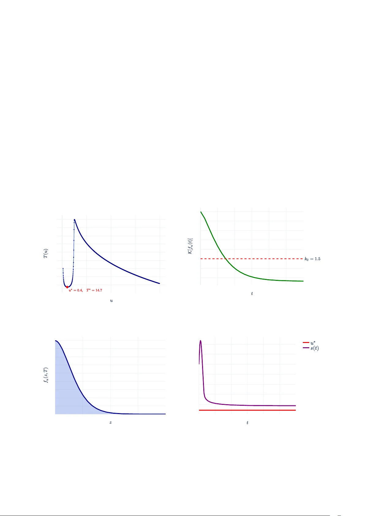
T AR GET CONTR OLLABILITY F OR A MINIMUM TIME PR OBLEM IN A TRAIT-STR UCTURED CHEMOST A T MODEL CLA UDIA AL V AREZ-LA TUZ, T ´ ERENCE BA YEN, AND J ´ ER ˆ OME CO VILLE Abstract. In this pap er, we consider a minim um time con trol problem gov erned by a trait- structured c hemostat mo del including mutation and one limiting substrate. Our first main result pro ves the w ell-p osedness of the con trol-to-state mapping. W e subsequently analyze the class of auxostat-typ e c ontr ols , feedback la ws designed to regulate substrate concentration, and pro ve that the corresponding solutions con verge to a stationary state of the system. These con vergence results are used to sho w the reachabilit y of a target set corresp onding to the selection of a p opulation with a low weigh ted av eraged half-saturation constan t. Finally , w e show the existence of an optimal control for the minimum time problem asso ciated with reac hing the target set. These theoretical findings are completed by n umerical simulations. 1. Introduction 1.1. General con text. Con tin uous culture can b e used to select through comp etition sp e- cific micro organisms of interest from a p o ol of sp ecies initially present or app earing by m u- tation. Since its in troduction in the fifties b y Monod [ 34 , 35 ] and No vik and Szilard [ 36 ], the chemostat system has found widespread applications ov er the past 75 y ears in a v ariet y of contexts [ 2 , 21 , 27 , 29 , 41 ]. In particular, it has provided v aluable insigh ts in microbiol- ogy in to the adaptive mechanisms in v olv ed in resp onses to controlled en vironmen ts (see, e.g. , [ 16 , 21 , 24 , 25 , 26 , 28 ]). Although c hemostat systems are for most of them designed to study a finite n um b er of p opulation, contin uous versions of it with infinitely man y t yp e of p opulation ha v e also been in tro duced, see [ 10 , 18 , 30 , 33 , 38 ]. In this spirit we consider here the growth of a p opulation structured by a phenot ypical trait z living in a limited substrate environmen t, all traits competing with each other through the access of the resource. A key asp ect of the mo del is that phenot ypical c hanges in the population are taken into account through the inclusion of m utation. F ollowing the modeling approach proposed by [ 9 , 10 , 14 , 18 , 30 , 33 , 38 ], the dynamics of this p opulation can b e represented b y the following set of in tegro-differential equations: (1.1) ∂ t f ( t, z ) = ( µ ( s ( t ) , z ) − u ( t )) f ( t, z ) + α ∆ z f ( t, z ) for t > 0 , z ∈ Ω , ˙ s ( t ) = − ˆ Ω µ ( s ( t ) , z ′ ) f ( t, z ′ ) dz ′ + u ( t )( s in − s ( t )) for t > 0 , ∂ n f ( t, z ) = 0 for t > 0 , z ∈ ∂ Ω , s (0) = s 0 > 0 , f (0 , z ) = f 0 ( z ) ≥ 0 for z ∈ Ω , where the function s is the substrate concen tration and the function f represen ts the density of the p opulation under consideration growing on the substrate. Here, the constan t s in > 0 is the input substrate concen tration, s 0 is the initial substrate concen tration, f 0 , the initial densit y of the p opulation, µ is the gro wth function (or kinetics) and the function u ≥ 0 is the dilution rate which serves as the control input for the system. The distinction b etw een the different sp ecies is made through the function µ which dep ends on the trait z ∈ Ω, where Ω is a b ounded domain of R d with smo oth b oundary and unit normal v ector n . The mutation pro cess, whic h can be interpreted as mov ement in the trait space, is here considered to b e driven by diffusion and is therefore mo deled b y the Laplace operator, where α ≥ 0 represents the mutation rate. Additionally , the Neumann b oundary condition reflects that the p opulation do es not conv ert in to or from traits beyond the limits of the domain. This w ork is dev oted to the analysis of ( 1.1 ), including existence and uniqueness of solutions, stabilization prop erties, reac habilit y of a given target set, and the asso ciated minimum-time con trol problem. 1 2 CLAUDIA AL V AREZ-LA TUZ, T ´ ERENCE BA YEN, AND J ´ ER ˆ OME COVILLE 1.2. Related mo dels. In the literature, n umerous results hav e b een established within the framew ork of adaptive dynamics, considering b oth deterministic and sto chastic settings. These include findings on the conv ergence of solutions to stationary states, as w ell as descriptions of the asymptotic limits as the m utation parameter α ↓ 0. Giv en the extensive scop e of existing w ork, w e highligh t here a selection of relev ant contributions. First, the article [ 11 ] inv estigates an extension of the competitive Lotk a-V olterra system and prov es con vergence to a unique stable equilibrium p oin t. Note also that concen tration phenomena in the limit of v anishing mutation rates are examined in [ 9 , 10 ], in b oth deterministic and sto chastic contexts. Another relev ant con tribution is the analysis of a non-lo cal Lotk a-V olterra m utation-comp etition mo del in [ 32 ]. In [ 18 ], a selection-mutation mo del with asymptotically small mutation parameter is s tudied based on the HJB equation. Extinction phenomena in a sto c hastic chemostat mo del are addressed in [ 12 ], while [ 33 ] studies a trait-structured c hemostat-type model and pro vides sufficien t conditions for p opulation surviv al. The relationship b etw een deterministic and sto chastic form ulations of the c hemostat is examined in [ 8 ]. Finally , it is worth men tioning [ 20 ] which studies a related mo del in whic h the m utation term differs : whereas we consider a Laplacian operator, m utation in [ 20 ] is modeled through a kernel function K ( z , z ′ ) represen ting the probabilit y densit y of the phenot yp e z ′ to be a m utant of (initial) phenot ype z (which is a non-lo cal operator). In addition, our work addresses optimal control questions. 1.3. A minimum time control problem. While existence and uniqueness of solutions in our setting follows from rather classical argumen ts, muc h less is known ab out con trollability and optimal control, particularly for mo del ( 1.1 ). T o study this, let us define an ob jective function. The ques tion is whether one can design an optimal con trol strategy , i.e. , an admissible control function u , optimizing a desired ob jective function. In the con text of ( 1.1 ), this ob jectiv e raises significan t c hallenges. The main aim of this article is therefore to clarify whether the system ( 1.1 ) can b e controlled, with the following minim um-time con trol problem in mind: Optimal Con trol Problem. L et F b e a set of initial c ondition for ( 1.1 ) to gether with a tar get set T 0 . Given ( s 0 , f 0 ) ∈ F , the go al is to find an optimal c ontr ol u such that the solution to ( 1.1 ) r e aches the tar get set T 0 in minimal time and stays in it for al l subse quent times, i.e., (1.2) inf u ∈U T u s . t . f ( t, · ) ∈ T 0 for all t ≥ T u , wher e U is the set of admissible c ontr ols and f the solution to ( 1.1 ) for the c ontr ol u . Optimization of the chemostat system, particularly through minimum-time problems, has man y practical applications in biopro cesses, suc h as wastew ater treatment and the selection of sp ecies of in terest from a mixed p opulation (see, e.g. , [ 5 , 6 , 19 ]). Other criteria, such as pro ductivit y , can also b e considered, as in [ 4 ]. In the present work, w e extend this line of inquiry to mo del ( 1.1 ), whic h incorporates a trait. In particular, w e c ho ose the target set T 0 follo wing the approach of [ 6 ], with the specific biological aim of se lecting p opulations of in terest (which is a common ob jectiv e in the con trol of biopro cesses). Minimum time problems in infinite-dimensional settings (see, e.g. , [ 23 , 31 , 43 , 44 ]) are generally more c hallenging than their finite-dimensional coun terparts. In the latter, the application of the Pon tryagin Maximum Principle and related tec hniques is standard, whereas their extension to infinite dimensions faces substan tial obstacles. One imp ortant asp ect of problem ( 1.2 ) is the nonlinearity of the state equation, in contrast with related works. Another distinctive feature of problem ( 1.2 ) is the requiremen t that the state, up on first reaching the target, must stay within it (see also [ 44 ]). This “reach-and-sta y” condition is more demanding than the classical reac habilit y requiremen t, y et we will sho w that it can b e achiev ed under suitable assumptions. 1.4. Notation and assumptions. The following notations will b e used throughout the paper. • The notations R + and R ∗ + refer to the interv als [0 , + ∞ ) and (0 , + ∞ ) resp ectiv ely . • The set Ω is a b ounded domain in R d ( d ≥ 1) with a smo oth b oundary (of class C 1 ) ; ∂ Ω and int(Ω) denote resp ectively its b oundary and its in terior. • Given a Borel set in R k , for k ≥ 1, | A | and 1 A stand for the Lebesgue measure of A and the indicator function of A , resp ectively . T ARGET CONTR OLLABILITY FOR A MINIMUM TIME IN CHEMOST A T MODEL 3 • B R and B R ( x ) denote the op en balls of radius R centered at 0 and x resp ectiv ely . • M (Ω) and M + (Ω) denote the spaces of finite signed and positive Radon measures on Ω, resp ectively . • F or brevity , w e will often write L p and L ∞ for the Leb esgue spaces L p (Ω) and L ∞ (Ω). • The L p -norm of a function g in L p (1 ≤ p < + ∞ ) is written ∥ g ∥ p := ´ Ω | g ( z ) | p dz 1 p . • C ( I ) is the Banac h space of con tin uous real-v alued functions on I . F or an in terv al J ⊂ R , C ( I , J ) denotes the subset of C ( I ) with v alues in J . • F or a Banac h space E , the set C ( I , E ) denotes contin uous functions with v alues in E . W e alert the reader that w e use b oth the notation C ( I , J ) (when J is an interv al) and C ( I , E ) when E is a Banac h space. • F or ( k , β ) ∈ N × (0 , 1), the set C k,β ( I , E ), resp. C k,β loc ( I , E ), denotes functions that are H¨ older contin uous, resp. lo cally H¨ older contin uous of order ( k , β ) with v alues in E . • F or ( k , β ) ∈ N × (0 , 1), C k,β (Ω), resp. C k,β loc (Ω), denotes real-v alued functions that are H¨ older contin uous, resp. lo cally H¨ older contin uous of order ( k , β ). • F or f , ˜ f ∈ C ( R , L 1 ), m ( t ) and ˜ m ( t ) stand for ∥ f ∥ 1 ( t ) and ∥ ˜ f ∥ 1 ( t ), resp ectively . • The admissible control set is U := { u : R + → [0 , u max ] | u meas. } with u max > 0. Admissible controls are denoted by u . • The time deriv ative of a function F : R → R is written ˙ F or d dt F ( t ). Returning to the mo deling assumptions (particularly that the growth function is alwa ys n ull in absence of substrate in a chemostat system), w e adopt the follo wing hypotheses for the kinetics. Hyp othesis 1.1. µ ∈ C 1 loc ( R + , C 1 (Ω)) ; µ ( s, · ) ∈ L ∞ (Ω) ∩ C 0 , 1 (Ω) for al l s > 0 ; µ ( s, z ) > 0 for al l ( s, z ) ∈ R ∗ + × ¯ Ω and µ (0 , z ) = 0 for al l z ∈ Ω . Additionally , w e imp ose the following b oundedness condition on the kinetics and a corre- sp onding Lipschitz assumption. Hyp othesis 1.2. Ther e exists ˆ µ > 0 such that for al l s ≥ 0 sup z ∈ Ω µ ( s, z ) ≤ ˆ µs, and for al l S ≥ 0 ther e is b S > 0 such that for al l s, s ′ ∈ [0 , S ] and for al l z ∈ Ω , | µ ( s, z ) − µ ( s ′ , z ) | ≤ b S | s − s ′ | . 1.5. Ov erview of the contribution and organization. This section presen ts the pap er’s main results in detail. 1.5.1. Existenc e r esults for ( 1.1 ) . T o prop erly handle the control problem, it is imp ortan t to study the input-output map, which associates a solution of the coupled system to a giv en control, and to sho w that it is well-defined. That is why , we will first establish in Section 2 the existence and uniqueness of p ositive (mild and classical) solutions to ( 1.1 ), giv en some admissible con trol. T o understand the difficulty of obtaining suc h results, assume for the momen t that the kinetics µ is of Mono d type, that is, (1.3) µ ( s, z ) := ¯ µs r ( z ) + s , where r ∈ C (Ω), r > 0 ov er Ω, and ¯ µ > 0. The problem ( 1.1 ) then rewrites: ∂ t f ( t, z ) = ¯ µs ( t ) r ( z ) + s ( t ) − u ( t ) f ( t, z ) + α ∆ z f ( t, z ) for t > 0 , z ∈ Ω , ˙ s = − ¯ µ ˆ Ω s ( t ) r ( z ′ ) + s ( t ) f ( t, z ′ ) dz ′ + u ( t )( s in − s ( t )) for t > 0 , ∂ n f ( t, z ) = 0 for t > 0 , z ∈ ∂ Ω , s (0) = s 0 > 0 , f (0 , z ) = f 0 ( z ) for z ∈ Ω . When the dilution rate u is smo oth, it is reasonable to think that the abov e nonlinear problem is w ell posed and that the solution will be smo oth thanks to the general parab olic theory . How ev er, 4 CLAUDIA AL V AREZ-LA TUZ, T ´ ERENCE BA YEN, AND J ´ ER ˆ OME COVILLE when u is only measurable (for instance, whenever u is of bang-bang type), this fact is not clear an ymore. Our first result is to define prop erly a solution to ( 1.1 ) and to show that for an y admissible con trol function, the system ( 1.1 ) admits a unique, well-defined solution. In this direction, our main result is as follo ws. The result is stated for arbitrary kinetics (not restricted to Mono d kinetics), pro vided suitable assumptions are satisfied. Theorem 1.1. Supp ose that α > 0 and that µ satisfies Hyp otheses 1.1 - 1.2 . Then, for every admissible c ontr ol u , and for every initial data s 0 ∈ (0 , s in ) and f 0 ∈ L 1 (Ω) such that f 0 ≥ 0 , ther e is a unique p air of p ositive functions ( s, f ) with s ∈ C 1 ( R ∗ + , [0 , s in ]) ∩ C ( R + , [0 , s in ]) and f ∈ C ( R + , L 1 (Ω)) ∩ C 0 , 1 loc ( R ∗ + , C 2 ,β (Ω) ∩ C 0 ,β ( ¯ Ω)) such that ( s, f ) is a mild solution to ( 1.1 ) . Mor e over, if u ∈ C ( R ) , then f is a str ong solution and f ∈ C 1 ( R ∗ + , C 2 ,β (Ω) ∩ C 0 ,β ( ¯ Ω)) . The pro of of this theorem is detailed in Section 2 . As we can see, there is a direct relation- ship b et w een the smo othness of the con trol and the smo othness of the resulting solution. In particular, whenev er u is piecewise con tin uous, then, the solution is a piecewise C 1 function of the time. When α = 0 the system ( 1.1 ) exhibits less regularity . Nev ertheless, the existence of a solution can still b e established, as stated b elo w. Theorem 1.2. Supp ose that α = 0 and that µ satisfies Hyp otheses 1.1 - 1.2 . Then, for every admissible c ontr ol u , and for every initial data s 0 ∈ (0 , s in ) and f 0 ∈ L 1 (Ω) such that f 0 ≥ 0 , ther e is a unique p air of non ne gative functions ( s, f ) with s ∈ C 1 ( R ∗ + , [0 , s in ]) ∩ C ( R + , [0 , s in ]) and f ∈ C ( R + , L 1 (Ω)) ∩ C 1 ( R ∗ + , L 1 (Ω)) such that ( s, f ) is a mild solution to ( 1.1 ) . In addition, supp( f ( t, · )) ⊂ supp( f 0 ) for al l t ≥ 0 . Remark 1. In con trast with Theorem 1.1 , the pro of of the previous statement follows from classical results in the literature using Cauch y-Lipschitz’s theory in Banac h spaces [ 7 , 17 , 39 ], therefore, we do not provide it here. 1.5.2. Stabilization r esults. Control theory frequen tly utilizes v arious input classes distinct from op en-lo op con trols, in particular those in v olving a measure of the state of the system. Therefore, in this pap er, we shall take adv antage of fe e db ack c ontr ols (closed-loop control functions) that dep end on the state of the system. Such con trols ma y b e used in several contexts suc h as to adjust the solution of a con trol system under deviations, to reduce sensitivit y of initial conditions, or to stabilize a dynamical system. In this framew ork, at eac h time instan t, a feedback con trol is determined by the current state of the system. In practical terms, the control may b e a function of time, space, and the state function itself. In Section 3 , w e examine conv ergence of solutions to ( 1.1 ) whenever the input is an auxostat-typ e c ontr ol , a particular type of feedbac k con trol. In biopro cesses, auxostats are designed to regulate the substrate concen tration at a desired set-point (see, e.g. , [ 6 ] in the context of the c hemostat system and Remark 3 ). W e shall see that, under suc h a con trol function, the system is driv en to wards a desired stationary state of ( 1.1 ). Thanks to these prop erties, auxostat-t yp e con trols will constitute a key to ol in Section 4 for proving the “reach and sta y” prop ert y of the desired giv en target set in the minim um-time problem ( 1.2 ), for Mono d kinetics. Let us then consider control functions that can b e expressed as a functional of the state, i.e. , u ( t ) := R [ f ( t, · ) , s ( t )] , t ≥ 0 , where R a contin uous functional ov er the space L 1 (Ω) × R + with v alues in R + . F or such a con trol function, we ha v e the following result. Theorem 1.3. Supp ose that α > 0 and that µ satisfies Hyp otheses 1.1 - 1.2 . Then, for every c ontr ol map t 7→ u ( t ) := R [ f ( t, · ) , s ( t )] and for every initial data s 0 ∈ (0 , s in ) and f 0 ∈ L 1 (Ω) such that f 0 ≥ 0 , ther e is a unique p air of p ositive functions ( s, f ) with s ∈ C 1 ( R ∗ + , [0 , s in ]) ∩ C ( R + , [0 , s in ]) and f ∈ C ( R + , L 1 (Ω)) ∩ C 0 , 1 loc ( R ∗ + , C 2 ,β (Ω) ∩ C 0 ,β ( ¯ Ω)) such that ( s, f ) is a mild solution to ( 1.1 ) . Mor e over, if u ∈ C ( R ) , then f is a str ong solution and f ∈ C 1 ( R ∗ + , C 2 ,β (Ω) ∩ C 0 ,β ( ¯ Ω)) . Remark 2. In con trast with Theorem 1.1 , we shall only sketc h the proof of the previous statemen t, which follo ws from classical results in the literature since t 7→ u ( t ) is no longer T ARGET CONTR OLLABILITY FOR A MINIMUM TIME IN CHEMOST A T MODEL 5 arbitrary , but a feedbac k of f and s [ 15 , 38 ]. It can also b e noticed that without a uniform b ound on the L 1 -norm of the solution f and the precise description of the b ehavior of s , such a control function may exceed any prescrib ed upp er b ound u max , making it p otentially not suitable to b e used for solving ( 1.2 ). Building on this result, Section 3 examines ho w auxostat-t ype controls u of the following form affect the b ehavior of the system: (i) u ( t ) = 1 s in − s ( t ) ˆ Ω µ ( s ( t ) , z ) f ( t, z ) dz , (ii) u ( t ) = 1 s in − σ ˆ Ω µ ( s ( t ) , z ) f ( t, z ) dz , (iii) u ( t ) = 1 s in − s ( t ) ˆ Ω µ ( σ, z ) f ( t, z ) dz , (iv) u ( t ) = 1 s in − σ ˆ Ω µ ( σ, z ) f ( t, z ) dz , where σ ∈ (0 , s in ) is a given key parameter. T o simplify notation, the dep endence of u on σ is omitted. Remark 3. Controls (i), (iii), and (iv) can be view ed as v ariants of con trol (ii), which represen ts the contin uous biogas output in a con tin uously stirred chemostat. This quan tit y is readily measurable in practice (see, e.g. , [ 6 ]). The terminology auxostat-typ e c ontr ols stems from the fact that, when control (iii) is substituted in to ( 1.1 ), the system satisfies the following property 1 : s ( t 0 ) = σ ⇒ ∀ t ≥ t 0 , ˙ s ( t ) = 0 , where t 0 is arbitrary . Thus, this control enables the regulation of the substrate concen tration at the desired v alue σ . As far as w e know, studying the effect of controls (i)-(ii)-(iii)-(iv) in to ( 1.1 ) has not b een addressed previously . F or such controls, Theorem 1.3 ensures the existence of a unique solution solution ( s, f ) to ( 1.1 ), whic h is w ell defined o ver R + × Ω. In Section 3 , w e establish the existence of a stationary solution of ( 1.1 ), parametrized by σ , around which the system is stabilized b y any of the three con trols (ii), (iii), or (iv), for all nonnegative initial data. F or the control given b y ( i ), the b eha vior of the system slightly differs, and w e hav e the following conv ergence result. Theorem 1.4. Supp ose that µ satisfies Hyp otheses 1.1 - 1.2 , that α > 0 , and that the c ontr ol u ( · ) is given by ( i ) . L et then ( s, f ) b e the unique solution to ( 1.1 ) asso ciate d with the initial data ( s 0 , u 0 ) wher e s 0 > 0 and f 0 ≥ 0 ( f 0 b eing non-nul l). Denote by ϕ s 0 a p ositive eigenfunction asso ciate d with the princip al eigenvalue λ 1 of the fol lowing sp e ctr al pr oblem: ( α ∆ ϕ ( z ) + µ ( s 0 , z ) ϕ ( z ) = − λϕ ( z ) for z ∈ Ω , ∂ n ϕ ( z ) = 0 for z ∈ ∂ Ω . Then for al l t ≥ 0 , s ( t ) = s 0 and for al l 1 ≤ p < + ∞ , one has: lim t → + ∞ f ( t, · ) − s in − s 0 ∥ ϕ s 0 ∥ 1 ϕ s 0 ( · ) p = 0 . The pro of of this theorem is detailed in Section 3.1 . As a result, the feedback giv en b y (i) driv es the solution of the system to a stationary solution parametrized by the initial condition. F rom an applicative standp oint, con trols of t yp e (ii), (iii), or (iv) are preferable as the limit solution is indep endent of the initial condition. F or each one of the three previous cases, the stabilization result can b e stated as follows, noting that it requires slightly stronger assumptions on the growth rate function. Theorem 1.5. Supp ose that µ satisfies Hyp otheses 1.1 - 1.2 , that α > 0 , and let σ ∈ (0 , s in ) . Denote by ϕ σ a p ositive eigenfunction asso ciate d with the princip al eigenvalue λ 1 of the fol lowing sp e ctr al pr oblem: ( α ∆ ϕ ( z ) + µ ( σ, z ) ϕ ( z ) = − λϕ ( z ) for z ∈ Ω , ∂ n ϕ ( z ) = 0 for z ∈ ∂ Ω . Assume further that at le ast one of the fol lowing assumptions holds: 1 This is straightforw ard from Cauc hy-Lipsc hitz’s Theorem. 6 CLAUDIA AL V AREZ-LA TUZ, T ´ ERENCE BA YEN, AND J ´ ER ˆ OME COVILLE • the c ontr ol u is given by (ii) and for al l s > 0 , ther e is c 0 ( s ) > 0 such that inf z ∈ Ω µ ( s, z ) ≥ c 0 ( s ) , • the c ontr ol u is given by (iii) and for al l s ≥ 0 , ther e is c 1 ( s ) > 0 such that inf z ∈ Ω ∂ s µ ( s, z ) ≥ c 1 ( s ) , • the c ontr ol u is given by (iv), for al l z ∈ Ω , µ ( · , z ) ∈ C 2 ( R + ) and µ is strictly c onc ave w.r.t. s , i.e., ∂ ss µ ( s, z ) < 0 for al l ( s, z ) ∈ [0 , s in ] × Ω . Then, the p air ( ¯ s, ¯ f ) := σ, ( s in − σ ) φ σ ∥ φ σ ∥ 1 is the unique stationary solution to ( 1.1 ) in which u is given by any of the thr e e c ontr ols that satisfy their c orr esp onding afor ementione d assump- tions. Mor e over, for any initial data ( s 0 , f 0 ) wher e s 0 > 0 and f 0 ≥ 0 ( f 0 b eing non-nul l), the unique solution ( s, f ) to ( 1.1 ) asso ciate d with the c orr esp onding c ontr ol c onver ges to ( σ, ¯ f ) in the fol lowing sense: for 1 ≤ p < + ∞ , one has lim t → + ∞ ∥ f ( t, · ) − ¯ f ( · ) ∥ p = 0 . The proof of this theorem is detailed in Section 3.2 . Theorem 1.5 is illustrated in Section 4.2 in the case (iv). Additionally , the three control functions may not b e alwa ys admissible, never- theless, in Sec tion 4 , we show how to construct admissible con trols inv olving auxostat controls of the form (iv). 1.5.3. T ar get c ontr ol lability r esults. W e no w turn to describing the results obtained in this pap er concerning the reachabilit y of a given target set by solutions of ( 1.1 ). This analysis relies in particular on the auxostat-type con trols in tro duced in the previous section. F or this purpose, we assume throughout this part that µ is of Mono d type, i.e. , it satisfies ( 1.3 ) where r ∈ C (Ω , R ∗ + ) is the so-called half-satur ation function and ¯ µ > 0 is the maximum growth rate. F or a giv en trait z , the half-saturation function r ( z ) is the substrate concentration at whic h the sp ecific gro wth rate reaches ¯ µ/ 2. It represents a measure of gro wth efficiency of the species on the substrate. F or instance, a lo w half-saturation means that the sp ecies can gro w w ell even if the substrate concen tration is lo w. The function r is the main comp onent of the definition of the target set to b e considered hereafter. T o introduce it precisely , let us consider the functional K [ ν ] := ´ Ω r ( z ) dν ( z ) ´ Ω dν ( z ) , o v er the set M + (Ω) (here, ν ∈ M + (Ω)). Next, we identify the p ositive cone of L 1 (Ω) as a subset of M + (Ω), and for f ∈ L 1 (Ω) in this p ositiv e cone, the functional K rewrites K [ f ] = ´ Ω r ( z ) f ( z ) dz ´ Ω f ( z ) dz , so that (1.4) r 0 := min z ∈ Ω r ( z ) ≤ K [ f ] ≤ max z ∈ Ω r ( z ) =: r 1 . The functional K represen ts the mean half-saturation for all sp ecies, weigh ted b y the abundance of eac h trait. F rom a mo deling viewp oin t, w e will b e in terested in main taining this v alue under a giv en threshold to ensure the selection of population having a low half-saturation, in order to ha v e a more efficien t use of the substrate (see also [ 6 ] for further explanations on suc h a selection pro cess). The idea b ehind the definition of the target set is then to imp ose an upp er b ound on K [ f ] for biological consideration. This leads to the following definition: T 0 := f ∈ L 1 | K [ f ] ≤ k 0 , where k 0 ∈ ( r 0 , r 1 ). If k 0 ≥ r 1 , the problem is immediate since for an y initial data and an y con trol, the corresp onding solution f b elongs to T 0 for all time t > 0, hence, T u = 0. Th us, any T ARGET CONTR OLLABILITY FOR A MINIMUM TIME IN CHEMOST A T MODEL 7 con trol u is optimal, that is wh y w e assume k 0 ∈ ( r 0 , r 1 ). W e no w sp ecify initial conditions for the minimum time problem. The set of admissible initial conditions is defined as F := (0 , s in ] × f ∈ L 1 (Ω) | ∃ ( κ, η ) ∈ R ∗ + × R ∗ + , ∀ z ∈ Ω , f ( z ) ≥ κ 1 B η ( ¯ x ) ∩ Ω ( z ) , where ¯ x ∈ arg min z ∈ ¯ Ω ( r ( z )). Note that for biological reasons s 0 > 0 and f 0 is nonnegativ e o ver Ω ( f 0 b eing non-zero). The set F consists of functions having a p ositive measure in a neigh b orho o d of the “leader trait”, i.e. , the trait corresp onding to the most efficient growth with respect to substrate consumption. F or the sp ecific class of Mono d kinetics, this is equiv alen t to minimizing r . This requirement implies that the initial biomass distribution must tak e p ositive v alues in a neighborho o d of the leader trait in order to guarantee the existence of an equilibrium when α = 0, as predicted b y the comp etitive exclusion principle [ 38 ]. T o address the minimum time con trol problem, we b egin by in v estigating the following target reac habilit y problem. Reac habilit y Problem. Given u max > 0 and k 0 ∈ ( r 0 , r 1 ) , find a c ontr ol u ∈ U and a finite time T ∈ (0 , + ∞ ) such that f ( t, · ) ∈ T 0 for al l t ≥ T , that is, ∀ t ≥ T , K [ f ( t, · )] ≤ k 0 . The main result of this section asserts that the target can alwa ys b e reached b y an admissible con trol provided that the m utation parameter is small enough. F or future reference, we set (1.5) υ := sup ( s,z ) ∈ [0 ,s in ] × Ω µ ( s, z ) and ¯ u := max( υ , 4 υ s in ) . Prop osition 1.6. L et u max ≥ ¯ u . Given k 0 ∈ ( r 0 , r 1 ) , ther e is α 0 such that for al l α ∈ [0 , α 0 ) and for al l initial data in F , ther e exists a c on tr ol u ∈ U such that the c orr esp onding solution to ( 1.1 ) enters the tar get set T 0 in finite time and r emains in T 0 for al l subse quent times. The pro of of this prop osition is detailed in Section 4.1 . 1.5.4. Minimum time r esults. Our last con tribution is dev oted to the study of ( 1.2 ) when α is small enough (in accordance to Prop osition 1.6 ). Based on the previous results, we establish the existence of an optimal con trol. Theorem 1.7. L et u max ≥ ¯ u . Given k 0 ∈ ( r 0 , r 1 ) , ther e is α 0 such that for al l α ∈ [0 , α 0 ) and for al l ( s 0 , f 0 ) ∈ F , the minimum-time pr oblem ( 1.2 ) admits an optimal c ontr ol u ∗ ∈ U such that the asso ciate d state ( f ∗ , s ∗ ) r e aches the tar get set T 0 in a time T ∗ . The pro of of this theorem is detailed in Section 5.1 . Finally , w e complement these theoretical results with n umerical sim ulations illustrating con v ergence of solutions under auxostat-t ype con trols in Section 4.2 , and sub-optimal solutions to the minim um time control problem in Section 5.2 . 2. Existence of solutions to ( 1.1 ) The goal of this section is to prov e Theorem 1.1 . 2.1. Reform ulation of the state equation. Before going any further, w e make some prelim- inary remarks on system ( 1.1 ). First, we extend the function µ ( · , z ) by con tin uit y to s ≤ 0 b y setting it equal to 0, and w e k eep the notation µ for this extension. Next, we rewrite system ( 1.1 ) in a more con v enient form. F or this purp ose, for t ≥ 0, let us set M ( t ) := s ( t ) − s in + m ( t ) , where m represents the total p opulation m ( t ) = ˆ Ω f ( t, z ) dz . A quick computation sho ws that M satisfies the follo wing Cauch y problem: (2.1) d dt M ( t ) = − u ( t ) M ( t ) , M (0) = s (0) − s in + m (0) , 8 CLAUDIA AL V AREZ-LA TUZ, T ´ ERENCE BA YEN, AND J ´ ER ˆ OME COVILLE and thus, for all time t ≥ 0, one has M ( t ) = M (0) e − ´ t 0 u ( τ ) dτ . As a remark, the total biomass concentration can b e written (2.2) m ( t ) = s in − s ( t ) + ( s (0) − s in + m (0)) e − ´ t 0 u ( τ ) dτ , t ≥ 0 . It follows that ( 1.1 ) is equiv alent to the follo wing system (in whic h the equation for f is time dep enden t) (2.3) ∂ t f ( t, z ) = [ µ ( M ( t ) + s in − m ( t ) , z ) − u ( t )] f ( t, z ) + α ∆ f ( t, z ) for z ∈ Ω , ∂ n f ( t, z ) = 0 for z ∈ ∂ Ω , f (0 , z ) = f 0 ( z ) ≥ 0 for z ∈ Ω , where t > 0. It is readily seen that f is a solution to ( 2.3 ) if and only if the function ˜ f ( t, x ) := e ´ t 0 u ( τ ) dτ f ( t, x ) is a solution to the system (2.4) ∂ t ˜ f ( t, z ) = µ M ( t ) + s in − M ( t ) M (0) ˜ m ( t ) , z ˜ f ( t, z ) + α ∆ ˜ f ( t, z ) for z ∈ Ω , ∂ n ˜ f ( t, z ) = 0 for z ∈ ∂ Ω , ˜ f (0 , z ) = f 0 ( z ) ≥ 0 for z ∈ Ω , where t > 0. Hence, solving ( 2.4 ) pro vides a solution to ( 2.3 ) and thus a solution to ( 1.1 ). In the remaining of this section, our aim is to construct of p ositive solution to ( 2.4 ). 2.2. Pro of of Theorem 1.1 . In this part, w e show the t wo next theorems. Note that Theorem 1.1 ab out existence and uniqueness of a solution to ( 1.1 ) follo ws from Theorem 2.2 b elow (the substrate s can indeed b e deduced from f via ( 2.2 )). Theorem 2.1. L et Ω ⊂ R d b e a b ounde d domain with a b oundary of class C 1 and let u ∈ L ∞ loc ( R + ) . Supp ose also that α > 0 and that µ satisfies Hyp otheses 1.1 - 1.2 . Then, for al l initial data f 0 ≥ 0 such that f 0 ∈ L 1 (Ω) , ther e exists a nonne gative function ˜ f ∈ C ( R + , L 1 (Ω)) ∩ C 1 ( R ∗ + , C 2 ,β (Ω) ∩ C 0 ,β ( ¯ Ω)) solution to ( 2.4 ) , for some β ∈ (0 , 1) . Assume temp orarily that Theorem 2.1 holds. By exploiting the relationship b et w een f and ˜ f , we deduce the follo wing result (whic h implies Theorem 1.1 ). Theorem 2.2. L et Ω ⊂ R d b e a b ounde d domain with a b oundary of class C 1 and let u ∈ L ∞ loc ( R + ) . Supp ose also that α > 0 and that µ satisfies Hyp otheses 1.1 - 1.2 . Then, for al l initial data f 0 ≥ 0 such that f 0 ∈ L 1 (Ω) , ther e exists a unique nonne gative solution f ∈ C ( R + , L 1 (Ω)) ∩ C 0 , 1 loc ( R ∗ + , C 2 ,β (Ω) ∩ C 0 ,β ( ¯ Ω)) solution to ( 2.3 ) for some β ∈ (0 , 1) . Mor e over, if u ∈ C ( R ) , then f ∈ C 1 ( R ∗ + , C 2 ,β (Ω) ∩ C 0 ,β ( ¯ Ω)) . Pr o of. The existence of a solution follows from Theorem 2.1 setting f ( t, z ) := e − ´ t 0 u ( τ ) dτ ˜ f ( t, z ) , ( t, z ) ∈ R ∗ + × Ω . It remains to show that the solution is unique. The regularit y prop erties of the solution f dep ends only on the regularity of the control u and, since for u ∈ L ∞ loc ( R ), the function t 7→ e ´ t 0 u ( τ ) dτ b elongs to the space 2 W 1 ,p loc ( R ) for all p ≥ 1 and is, in particular, lo cally Lip chitz, we deduce that f ∈ C 0 , 1 loc ( R ∗ + , C 2 ,β (Ω) ∩ C 0 ,β ( ¯ Ω)) ∩ C ( R + , L 1 (Ω)). Supp ose there exist tw o distinct positive solutions f 1 ( t, z ) , f 2 ( t, z ) to ( 2.3 ) with iden tical initial data. Then the corresponding functions 2 It is the space of real-v alued functions on R suc h that, on ev ery b ounded in terv al, the function and its first w eak deriv ative b elong to L p ( R ). T ARGET CONTR OLLABILITY FOR A MINIMUM TIME IN CHEMOST A T MODEL 9 ˜ f 1 , ˜ f 2 solv e ( 2.4 ) and inherit the same initial data. By in tegrating ( 2.4 ) with resp ect to z , the function ˜ m i = ∥ ˜ f i ∥ 1 satisfies: d dt ˜ m i ( t ) = ˆ Ω µ M ( t ) + s in − M ( t ) M (0) ˜ m i ( t ) , z ˜ f i ( t, z ) dz , ˜ m i (0) = m (0) , for i = 1 , 2. By definition of M , we also ha ve M ( t ) M (0) = e − ´ t 0 u ( τ ) dτ , (2.5) M ( t ) + s in = M (0) e − ´ t 0 u ( τ ) dτ + s in = ( m (0) + s 0 ) e − ´ t 0 u ( τ ) dτ + s in 1 − e − ´ t 0 u ( τ ) dτ , (2.6) for all t ≥ 0, and th us, for i = 1 , 2: (2.7) ∀ t ≥ 0 , M ( t ) + s in − M ( t ) M (0) ˜ m i < s in + s 0 + m (0) . Let us now define a function h : R + → R as h ( t ) := ˆ Ω [ ˜ f 1 ( t, z ) − ˜ f 2 ( t, z )] dz = ˜ m 1 ( t ) − ˜ m 2 ( t ) , t ≥ 0 . W e hav e h (0) = 0 and, using ( 2.4 ), we deduce that for all t > 0, ˙ h ( t ) = ˆ Ω µ M ( t ) + s in − M ( t ) M (0) ˜ m 1 ( t ) , z ˜ f 1 ( t, z ) dz − ˆ Ω µ M ( t ) + s in − M ( t ) M (0) ˜ m 2 ( t ) , z ˜ f 2 ( t, z ) dz =: rhs( t ) No w since µ satisfies Hyp otheses 1.1 - 1.2 , there is C ≥ 0 such that for all t ≥ 0, µ M ( t ) + s in − M ( t ) M (0) ˜ m 1 ( t ) , z − µ M ( t ) + s in − M ( t ) M (0) ˜ m 2 ( t ) , z ≤ C M ( t ) M (0) | h ( t ) | , and, therefore, by using ( 2.5 ) and ( 2.7 ), the expression rhs( t ) can b e estimated as follo ws: | rhs( t ) | ≤ C | h ( t ) | ˜ m 1 ( t ) + ˆ Ω µ M ( t ) + s in − M ( t ) M (0) ˜ m 2 ( t ) , z ( ˜ f 1 ( t, z ) − ˜ f 2 ( t, z )) dz ≤ C | h ( t ) | ˜ m 1 ( t ) + C 0 | h ( t ) | , t ≥ 0 , where (2.8) C 0 := sup ( s,z ) ∈ Λ µ ( s, z ) with Λ := [0 , s in + s 0 + m (0)] × Ω . Th us, the function h satisfies ∀ t > 0 , | ˙ h ( t ) | ≤ ( C ˜ m 1 ( t ) + C 0 ) | h ( t ) | . F rom the ab ov e differential inequality and b y using Gr¨ on w all’s inequalit y , we can see that h ( t ) = 0 for all t ≥ 0. As a consequence w e ha v e ˜ m 1 ( t ) = ˜ m 2 ( t ) for all t ≥ 0 and thus also m 1 ( t ) = m 2 ( t ) for all t ≥ 0. Let us no w set w := f 1 − f 2 . A quick calculation yields (2.9) ∂ t w ( t, z ) = [ µ ( M ( t ) + s in − m 1 ( t ) , z ) − u ( t )] w ( t, z ) + α ∆ z w ( t, z ) for z ∈ Ω , ∂ n w ( t, z ) = 0 for z ∈ ∂ Ω , w (0 , z ) = 0 for z ∈ Ω , for all t > 0. Hence, by applying the w eak parabolic maxim um principle w e get w ( t, z ) ≤ 0 for all ( t, z ) ∈ R ∗ + × Ω. Interc hanging the roles of f 1 , f 2 , we also get − w ( t, z ) ≤ 0 for all ( t, z ) ∈ R ∗ + × Ω. W e conclude that f 1 ( t, z ) = f 2 ( t, z ) for all ( t, z ) ∈ R ∗ + × Ω as w anted. □ W e now turn to the pro of of Theorem 2.1 . 10 CLAUDIA AL V AREZ-LA TUZ, T ´ ERENCE BA YEN, AND J ´ ER ˆ OME COVILLE Pr o of of The or em 2.1 . First, observe that, since u ∈ L ∞ loc ( R ), the function t 7→ e ´ t 0 u ( τ ) dτ b elongs to the space W 1 ,p loc ( R ) for all p ≥ 1, and, in particular, it is H¨ older contin uous. T o construct a solution to ( 2.4 ), w e will follow standard appro ximation techniques. The rest of the proof is divided into tw o steps. Step 1: Existenc e of a solution for a r e gularize d initial c ondition. First, we regularize f 0 b y a smo oth m ollifier ( ρ ε ) ε with unit mass and we consider ( 2.4 ) together with the initial condition f 0 ,ε := ρ ε f 0 in place of f 0 . Next, for ε > 0 fixed, let us introduce a sequence of function ( ˜ f n,ε ) n ∈ N suc h that ˜ f 0 ,ε = f 0 ,ε and where for n ∈ N ∗ , the function ˜ f n,ε is defined recursively by (2.10) ∂ t ˜ f n,ε ( t, z ) = c n ( t, z ) ˜ f n,ε ( t, z ) + α ∆ z ˜ f n,ε ( t, z ) for t > 0 , z ∈ Ω , ∂ n ˜ f n,ε ( t, z ) = 0 for z ∈ ∂ Ω , ˜ f n,ε (0 , z ) = f 0 ,ε ( z ) ≥ 0 for z ∈ Ω , where the function c n is defined by 3 : (2.11) c n ( t, z ) := µ M ( t ) + s in − M ( t ) M (0) ˜ m n − 1 ,ε ( t ) , z for ( t, z ) ∈ R + × Ω . Since b y definition f 0 ,ε ∈ C ∞ (Ω), M ∈ C 0 , 1 ( R ) ∩ L ∞ (Ω), and µ is Lipschitz-con tinuous, from the standard parabolic theory (see, e.g. , [ 22 , 45 ]), the sequence ( ˜ f n,ε ) n ∈ N is well defined, that is, for each n ∈ N ∗ there is a unique smo oth solution ˜ f n,ε to ( 2.10 ) that b elongs to the space E β for some β ∈ (0 , 1) where E β := C ( R + ; C 2 ,β (Ω) ∩ C 0 ,β ( ¯ Ω)) ∩ C 1 ( R ∗ + ; C 2 ,β (Ω) ∩ C 0 ,β ( ¯ Ω)) . Moreo v er since f 0 ,ε ≥ 0 and for each n ∈ N , the null function is a sub-solution to ( 2.10 ), a straigh tforw ard application of the parab olic comparison principle, yields ˜ f n,ε ≥ 0 for all n ∈ N . F rom Hyp othesis 1.2 and using that ˜ f n,ε ≥ 0 for all n ∈ N , we deduce that (2.12) ∀ n ∈ N ∗ , ∀ t ≥ 0 , M ( t ) + s in − M ( t ) M (0) ˜ m n − 1 ,ε < s in + s 0 + m (0) , as for proving ( 2.7 ). Consequently , for all n ∈ N , ˜ f n,ε satisfies ∂ t ˜ f n,ε ( t, z ) ≤ C 0 ˜ f n,ε ( t, z ) + α ∆ z ˜ f n,ε ( t, z ) for t > 0 , z ∈ Ω , ∂ n ˜ f n,ε ( t, z ) = 0 for t > 0 , z ∈ ∂ Ω , ˜ f n,ε (0 , z ) = f 0 ,ε ( z ) ≥ 0 for z ∈ Ω , where C 0 is given by ( 2.8 ). By applying again the parab olic comparison principle, we get (2.13) ∀ n ∈ N ∗ , ∀ ( t, z ) ∈ R ∗ + × Ω , ˜ f n,ε ( t, z ) ≤ e C 0 t v ε ( t, z ) , where v ε is the unique solution of the diffusion equation ∂ t v ε ( t, z ) = α ∆ z v ε ( t, z ) for t > 0 , z ∈ Ω , ∂ n v ε ( t, z ) = 0 for t > 0 , z ∈ ∂ Ω , v ε (0 , z ) = f 0 ,ε ( z ) ≥ 0 for z ∈ Ω . Observ e that from the comparison principle, we also hav e ∥ v ε ∥ ∞ ( t ) ≤ ∥ f 0 ,ε ∥ ∞ for all t ≥ 0. Therefore, we deduce that for all T > 0 and all n ∈ N , ∀ ( t, z ) ∈ [0 , T ] × Ω , f n,ε ( t, z ) ≤ e C 0 T ∥ f 0 ,ε ∥ ∞ . As a result, since µ satisfies Hyp othesis 1.1 , ( 2.12 ) implies that there is C ′ ≥ 0 such that (2.14) ∀ n ∈ N , ∀ ( t, z ) ∈ [0 , T ] × Ω , F n ( t, z ) := | c n ( t, z ) ˜ f n ( t, z ) | ≤ C ′ e C 0 T ∥ f 0 ,ε ∥ ∞ . 3 Naturally , ˜ m n,ε = ∥ ˜ f n,ε ∥ 1 , and in the following, m ε = ∥ f ε ∥ 1 . T ARGET CONTR OLLABILITY FOR A MINIMUM TIME IN CHEMOST A T MODEL 11 Let us rewrite ( 2.10 ) as follo ws: ∂ t ˜ f n,ε − α ∆ ˜ f n,ε = F n ( t, z ) for t > 0 , z ∈ Ω , ∂ n ˜ f n,ε ( t, z ) = 0 for t > 0 , z ∈ ∂ Ω , ˜ f ε ( n, z ) = f 0 ,ε ( z ) ≥ 0 for z ∈ Ω . Since for all T > 0 , F n b elongs to the space L ∞ ([0 , T ] × ¯ Ω), b y standard parab olic L p estimates (see [ 45 , Theorem 9.2.2]), w e deduce that for all T > 0 and all p ≥ 1, ˜ f n,ε is now b ounded indep enden tly of n in the space W 1 , 2 ,p Q T ∩ W 1 , 1 ,p 0 Q T , where Q T := (0 , T ) × Ω and W 1 , 2 ,p Q T and W 1 , 1 ,p 0 Q T denote the t -anisotropic Sob olev spaces defined resp ectiv ely by: W 1 , 2 ,p Q T := u ∈ L p ( Q T ) | ∂ t u, ∇ u, and ∂ ij u ∈ L p ( Q T ) , for all 1 ≤ i, j ≤ d , W 1 , 1 ,p 0 Q T := u ∈ L p ( Q T ) | ∂ n u = 0 on ∂ Ω and ∂ t u, ∇ u ∈ L p ( Q T ) . The embedding W 1 , 2 ,p Q T → C 0 , β 2 [0 , T ] , C 0 ,β ( ¯ Ω) (whic h is v alid for p > n +2 2 and 0 < β < 2 − n +2 p , see, e.g. , [ 45 , Theorem 1.4.1]) implies the existence of β ∈ (0 , 1) such that the sequence ( ˜ f n,ε ) n ∈ N is uniformly b ounded in the space C 0 , β 2 [0 , T ] , C 0 ,β ¯ Ω . As a result, from the definition of F n , we see that F n is b ounded in C 0 , β 2 [0 , T ] , C 0 ,β ( ¯ Ω) indep enden tly of n , therefore, b y using Schauder estimates, the sequence ( ˜ f n,ε ) n ∈ N is uniformly b ounded in C 1 , β 2 ((0 , T ) , C 2 ,β (Ω) ∩ C 0 ,β ( ¯ Ω)) for eac h T > 0. By a diagonal extraction pro cedure, using the compact em b edding C 1 , β ′ 2 ((0 , T ) , C 2 ,β ′ (Ω) ∩ C 0 ,β ′ ( ¯ Ω)) → C 1 , β 2 ((0 , T ) , C 2 ,β (Ω) ∩ C 0 ,β ( ¯ Ω)), for an y β ′ < β there exists a subsequence ( ˜ f n k ,ε ) k ∈ N whic h con verges to a non-negative function ˜ f ε ∈ C 1 , β ′ 2 ( R ∗ + , C 2 ,β ′ (Ω) ∩ C 0 ,β ′ ( ¯ Ω)) ∩ C ( R + , C 2 ,β ′ (Ω) ∩ C 0 ,β ′ ( ¯ Ω)) that is a solution to ( 2.4 ) considering f 0 ,ε as the initial condition. As a byproduct, w e hav e ˜ f ε ≤ e C 0 t v ε . As the parameter ε > 0 w as arbitrary in the ab ov e construction, we ha v e obtained a solution ˜ f ε to ( 2.4 ) with initial condition f 0 ,ε for any ε > 0. Step 2: Pr o of of the existenc e of a solution to ( 2.4 ) with the initial c ondition f 0 . F or this purp ose, let ( ε n ) b e such that ε n ↓ 0 and consider the sequence of functions ( ˜ f ε n ). W e next sho w that this sequence is relatively compact in a suitable Banach space and that, up to a subsequence, it conv erges to a desired solution. First, we claim that for eac h T > 0, ˜ f ε is b ounded in the space C 1 , β 2 ((0 , T ] , C 2 ,β (Ω) ∩ C 0 ,β ( ¯ Ω)) indep enden tly of ε , for some 0 < β < 1. Going back to ( 1.1 ), w e see that s ε ( t ) satisfies ˙ s ε ( t ) = − ˆ Ω µ ( s ε ( t ) , z ) f ε ( t, z ) dz + u ( t )( s in − s ε ( t )) , for t ≥ 0. Note that for all t ≥ 0, one has s ε ( t ) ≥ 0 for all ε > 0. This follows using that s ε (0) = s 0 > 0, f ε ≥ 0, and Hypotheses 1.1 and 1.2 . As a consequence, we deduce that ∀ t ≥ 0 , 0 ≤ m ε ( t ) ≤ M ( t ) + s in ≤ m (0) + s 0 + s in . By integrating ( 2.3 ) ov er Ω, w e find that for all t > 0, one has: | ˙ m ε ( t ) | = ˆ Ω µ ( M ( t ) + s in − m ε ( t ) , z ) f ε ( t, z ) dz − u ( t ) m ε ( t ) ≤ ( C 0 + u ( t )) m ε ( t ) . Therefore, m ε is uniformly Lip chitz-con tinuous ov er (0 , T ). F rom this fact, combined to Hy- p othesis 1.2 and the fact that the function M is uniformly Lip chitz-con tinuous indep endently of ε , we th us deduce that the follo wing quantit y c ε , defined by c ε ( t, z ) := µ M ( t ) + s in − M ( t ) M (0) ˜ m ε ( t ) , z for ( t, z ) ∈ R + × Ω , is uniformly b ounded and Lipsc hitz-con tinous in time and space, indep endently of ε . No w, Ω b eing a smo oth domain, the Neumann heat k ernel generates a strongly con tin uous semigroup of 12 CLAUDIA AL V AREZ-LA TUZ, T ´ ERENCE BA YEN, AND J ´ ER ˆ OME COVILLE con tractions on L 1 (Ω) (see [ 7 , 37 ]), th us, there exists C > 0 such that: ∀ ( t, z ) ∈ R ∗ + × Ω , | v ε ( t, z ) | ≤ C t − d 2 ∥ f 0 ,ε ∥ 1 ≤ C t − d 2 ∥ f 0 ∥ 1 . As a result, for an y δ > 0 w e can find a constan t C ( δ ) suc h that for all t ≥ δ and all z ∈ Ω, one has v ε ( t, z ) ≤ C ( δ ). The preceding prop erty implies that for all δ > 0 and all T > δ , ( ˜ f ε ) is uniformly b ounded indep enden tly of ε in the set Q δ T = ( δ, T ) × Ω and that c ε ˜ f ε is also uniformly b ounded in Q δ T indep enden tly of ε . By using standard parab olic L p estimates ([ 45 , 9.2.2]), it follo ws that for all T > δ and all p ≥ 1, ( ˜ f ε ) is b ounded indep enden tly of ε in W 1 , 2 ,p Q δ T ∩ W 1 , 1 ,p 0 Q δ T . By using the em b edding W 1 , 2 ,p Q δ T → C 0 , β 2 [ δ, T ] , C 0 ,β ( ¯ Ω) for p > n +2 2 and 0 < β < 2 − n +2 p (see [ 45 , Theorem 1.4.1]) together with Schauder estimates, we conclude that ( ˜ f ε ) is bounded in C 1 , β 2 [ δ, T ] , C 2 ,β (Ω) ∩ C 0 ,β (Ω) for some β ∈ (0 , 1). This ends up the pro of of our claim. Finally , let us consider a sequence of p ositive num bers ( δ n ) suc h that δ n ↓ 0 as n → + ∞ . By using a diagonal extraction pro cedure and the claim, there exist β ′ ∈ (0 , β ) and a subsequence ( ˜ f ε n k ) k ∈ N whic h conv erges to a smo oth nonnegative solution ˜ f of ( 2.4 ) ov er Q T , with initial condition f 0 and such that ˜ f ∈ C 1 , β ′ 2 (0 , T ) , C 2 ,β ′ (Ω) ∩ C 0 ,β ′ ( ¯ Ω) ∩ C ([0 , T ] , L 1 (Ω)) . Since T is arbitrary , we conclude that ˜ f ∈ C 1 , β ′ 2 R ∗ + , C 2 ,β ′ (Ω) ∩ C 0 ,β ′ ( ¯ Ω) ∩ C ( R + , L 1 (Ω)). □ 3. St abiliza tion by aux ost a t-type controls In this section, we address asymptotical prop erties of ( 1.1 ) when the control u is an auxostat- t yp e control giv en by: (i) u ( t ) = 1 s in − s ( t ) ˆ Ω µ ( s ( t ) , z ) f ( t, z ) dz , (ii) u ( t ) = 1 s in − σ ˆ Ω µ ( s ( t ) , z ) f ( t, z ) dz , (iii) u ( t ) = 1 s in − s ( t ) ˆ Ω µ ( σ, z ) f ( t, z ) dz , (iv) u ( t ) = 1 s in − σ ˆ Ω µ ( σ, z ) f ( t, z ) dz , where σ ∈ (0 , s in ) is given. Additionally , from now on, the initial data is tak en in the set (3.1) D := (0 , s in ) × f 0 ∈ L 1 (Ω) | f 0 ≥ 0 and ˆ Ω f 0 ( z ) dz > 0 . 3.1. Con trol of the form (i). In this part, we pro ve Theorem 1.4 . T o this end, observ e that the control defined in ( i ) gives ˙ s = 0 and therefore, s ( t ) = s 0 for all time t ≥ 0. It follows that ∀ t ≥ 0 , u ( t ) = 1 s in − s 0 ˆ Ω µ ( s 0 , z ) f ( t, z ) dz , and, consequently , f satisfies : ∂ t f ( t, z ) = µ ( s 0 , z ) − 1 s in − s 0 ˆ Ω µ ( s 0 , z ′ ) f ( t, z ′ ) dz ′ f ( t, z ) + α ∆ z f ( t, z ) for t > 0 , z ∈ Ω , ∂ n f ( t, z ) = 0 for t > 0 , x ∈ ∂ Ω , f (0 , z ) = f 0 ( z ) ≥ 0 for z ∈ Ω . The function m ( t ) := ´ Ω f ( t, z ) dz then satisfies: ˙ m ( t ) = 1 − m ( t ) s in − s 0 ˆ Ω µ ( s 0 , z ) f ( t, z ) dz o v er R ∗ + . F or initial conditions f 0 ∈ D , a quick analysis shows that m ( t ) → s in − s 0 as t → + ∞ . On the other hand, thanks to [ 14 , 30 , 33 ], w e know that for any 1 ≤ p < + ∞ , f ( t, x ) → ( s in − s 0 ) φ s 0 ∥ φ s 0 ∥ 1 in L p (Ω) as t → + ∞ , where ϕ s 0 is a p ositiv e eigenfunction asso ciated with T ARGET CONTR OLLABILITY FOR A MINIMUM TIME IN CHEMOST A T MODEL 13 the first eigenv alue λ 1 ( α ∆ + µ ( s 0 , z )) and Neumann b oundary condition. More precisely , ϕ s 0 satisfies ( α ∆ ϕ s 0 + µ ( s 0 , z ) ϕ s 0 + λ 1 ϕ s 0 = 0 for all z ∈ Ω , ∂ n ϕ ( z ) = 0 for all z ∈ ∂ Ω . This ends up the pro of of Theorem 1.4 . Remark 4. In case (i), the solution f can be made explicit: f ( t, z ) = Ψ( t, z ) w ( t, z ) 1 + ´ t 0 ´ Ω µ ( s 0 ,z ) s in − s 0 Ψ( s, z ) w ( s, z ) dz ds , where Ψ := e − λ 1 t ϕ s 0 and w ( t, z ) = e t L h f 0 ( z ) φ s 0 ( z ) i for ( t, z ) ∈ R + × Ω. Here e t L stands for the Neumann diffusion semi-group generated b y the elliptic op erator L [ w ] := α φ 2 s 0 ∇ · ϕ 2 s 0 ∇ w . 3.2. Con trols of the form (ii), (iii) and (iv). The goal now is to pro v e Theorem 1.5 . W e start by proving the following lemma. Lemma 3.1. L et σ ∈ (0 , s in ) and µ satisfying Hyp otheses 1.1 - 1.2 . Assume further that at le ast one of the fol lowing assumption holds: • u is given by (ii) and for al l s > 0 , ther e is c 0 ( s ) > 0 such that inf z ∈ Ω µ ( s, z ) ≥ c 0 ( s ) > 0 , • u is given by (iii) and for al l s ≥ 0 , ther e is c 1 ( s ) > 0 such that inf z ∈ Ω ∂ s µ ( s, z ) ≥ c 1 ( s ) > 0 , • u is given by (iv) and for al l z ∈ Ω , µ ( · , z ) ∈ C 2 ( R + ) and is strictly c onc ave in s , i.e., ∂ ss µ ( s, z ) < 0 for all ( s, z ) ∈ [0 , s in ] × Ω . L et ( s 0 , f 0 ) ∈ D . Then, the unique solution ( s, f ) of ( 1.1 ) with the c orr esp onding c ontr ol satisfies lim t → + ∞ s ( t ) = σ and lim t → + ∞ m ( t ) = s in − σ. Remark 5. The preceding conditions are satisfied if µ is of Mono d type. Additionally , thanks to the b ehavior of s and the uniform bounds on the L 1 -norm of f , one can show that the abov e auxostat-t yp e controls are admissible if u max is chosen large enough. Pr o of. W e treat the three cases separately and, for conv enience, we start b y (ii). Case where u is giv en b y ( ii ) . In that case, for all ( t, z ) ∈ R ∗ + × Ω, ( 1.1 ) rewrites ∂ t f ( t, z ) = µ ( s ( t ) , z ) − 1 s in − σ ˆ Ω µ ( s ( t ) , z ′ ) f ( t, z ′ ) dz ′ f ( t, z ) + α ∆ f ( t, z ) t > 0 , z ∈ Ω , ˙ s ( t ) = − ˆ Ω µ ( s ( t ) , z ) f ( t, z ) dz + s in − s ( t ) s in − σ ˆ Ω µ ( s ( t ) , z ) f ( t, z ) dz t > 0 , ∂ n f ( t, z ) = 0 t > 0 , z ∈ ∂ Ω , s (0) = s 0 > 0 , f (0 , z ) = f 0 ( z ) ≥ 0 z ∈ Ω . By rearranging the terms of the second expression and in tegrating the first one o ver Ω, w e get: ˙ s ( t ) = − 1 + s in − s ( t ) s in − σ ˆ Ω µ ( s ( t ) , z ) f ( t, z ) dz t > 0 , ˙ m ( t ) = ˆ Ω µ ( s ( t ) , z ) f ( t, z ) dz 1 − m ( t ) s in − σ t > 0 . Since ( s 0 , f 0 ) ∈ D , the quantities µ ( s ( t ) , z ) and f ( t, z ) remain p ositive. Using the ODE 4 satisfied b y s , we hav e ˙ s ( t ) > 0 when s ( t ) < σ and ˙ s ( t ) < 0 when s ( t ) > σ . Moreov er, if there is t 0 ≥ 0 such that s ( t 0 ) = σ , then, by Cauc h y-Lipsc hitz’s Theorem, we ha ve s ( t ) = σ for all t ≥ t 0 . 4 ordinary differential equation 14 CLAUDIA AL V AREZ-LA TUZ, T ´ ERENCE BA YEN, AND J ´ ER ˆ OME COVILLE Similarly , w e find that ˙ m ( t ) > 0 when m ( t ) < s in − σ and that ˙ m ( t ) < 0 when m ( t ) > s in − σ . F rom this, w e deduce the following inequalities: max( σ, s 0 ) ≥ s ( t ) ≥ min( σ, s 0 ) and max( s in − σ, m (0)) ≥ m ( t ) ≥ min( s in − σ, s 0 ) for all t ≥ 0. By contin uity of inf Ω µ ( s, · ) with resp ect to s and from the previous estimates on s , we deduce that there exist constants C 2 ≥ 0 and C 3 ≥ 0 such that ∀ t ≥ 0 , ∀ z ∈ Ω , 0 ≤ C 2 ≤ µ ( s ( t ) , z ) < C 3 . Moreo v er, w e hav e C 2 > 0 since s 0 > 0. Going bac k to the ODEs satisfied resp ectively by s and m , we conclude that s ( t ) → σ and m ( t ) → s in − σ as t → + ∞ . Case where u is giv en b y ( iii ) . In that case, for all t > 0 and all z ∈ Ω, ( 1.1 ) rewrites ∂ t f ( t, z ) = µ ( s ( t ) , z ) − 1 s in − s ( t ) ˆ Ω µ ( σ, z ′ ) f ( t, z ′ ) dz ′ f ( t, z ) + α ∆ f ( t, z ) t > 0 , z ∈ Ω , ˙ s ( t ) = − ˆ Ω µ ( s ( t ) , z ) f ( t, z ) dz + s in − s ( t ) s in − s ( t ) ˆ Ω µ ( σ, z ) f ( t, z ) dz t > 0 , ∂ n f ( t, z ) = 0 t > 0 , z ∈ ∂ Ω , s (0) = s 0 > 0 , f (0 , z ) = f 0 ( z ) ≥ 0 z ∈ Ω . By rearranging the terms of the second expression, w e find that ˙ s ( t ) = ˆ Ω [ µ ( σ, z ) − µ ( s ( t ) , z )] f ( t, z ) dz = ( σ − s ( t )) ¨ ˜ K ∂ s µ ( τ σ + (1 − τ ) s ( t ) , z ) f ( t, z ) dτ dz , where ˜ K := Ω × [0 , 1]. Since ∂ s µ ( τ , z ) > 0 and f > 0, we deduce as previously that ˙ s ( t ) > 0 when s ( t ) < σ and that ˙ s ( t ) < 0 when s ( t ) > σ . Moreo v er, if there is t 0 ≥ 0 such that s ( t 0 ) = σ , and thus we ha ve s ( t ) = σ for all t ≥ t 0 . As a consequence, for all t ≥ 0 , max( σ, s 0 ) ≥ s ( t ) ≥ min( σ, s 0 ) . T o conclude, it remains to establish upp er and low er b ounds for the ab o ve double in tegral aw a y from zero. Integrating o v er Ω the equation satisfied b y f yields (3.2) ˙ m ( t ) = ˆ Ω µ ( s ( t ) , z ) f ( t, z ) dz − m ( t ) s in − s ( t ) ˆ Ω µ ( σ, f ( t, z )) dz , t ≥ 0 . No w assume that s 0 > σ . It follo ws that s is decreasing and since µ is increasing in s , we obtain the following differential inequalities: ˙ m ( t ) ≥ ˆ Ω µ ( σ, z ) f ( t, z ) dz 1 − m ( t ) s in − s 0 , ˙ m ( t ) ≤ m ( t ) sup z ∈ Ω µ ( s 0 , z ) − inf z ∈ Ω µ ( σ, z ) s in − σ m ( t ) , from which we deduce that for all t ≥ 0 , max m (0) , sup z ∈ Ω µ ( s 0 , z ) inf z ∈ Ω µ ( σ, z ) ( s in − σ ) ≥ m ( t ) ≥ min ( m (0) , ( s in − s 0 )) . Lik ewise, when s 0 < σ , s is increasing and from ( 3.2 ), we obtain for all t ≥ 0 ˙ m ( t ) ≥ ˆ Ω µ ( σ, z ) f ( t, z ) dz inf z ∈ Ω µ ( s 0 , z ) − sup z ∈ Ω µ ( σ, z ) m ( t ) s in − σ , ˙ m ( t ) ≤ ˆ Ω µ ( σ, z ) f ( t, z ) dz 1 − m ( t ) s in − s 0 , from which we deduce that for all t ≥ 0 max ( m (0) , s in − s 0 ) ≥ m ( t ) ≥ min m (0) , inf z ∈ Ω µ ( s 0 , z ) sup z ∈ Ω µ ( σ, z ) ( s in − σ ) . T ARGET CONTR OLLABILITY FOR A MINIMUM TIME IN CHEMOST A T MODEL 15 F rom the low er and upp er b ounds on s ( t ) and since for all τ ∈ [0 , 1], ∂ s µ ( τ , z ) > C 1 ( τ ) (uniformly in z ), there exist p ositiv e constants C 4 and C 5 suc h that ∀ τ ∈ [0 , 1] , ∀ t ≥ 0 , ∀ z ∈ Ω , C 4 ≤ ∂ s µ ( τ σ + (1 − τ ) s ( t ) , z ) ≤ C 5 . Com bining with the lo w er and upp er b ounds on m yields ¨ ˜ K ∂ s µ ( τ σ + (1 − τ ) s ( t ) , z ) f ( t, z ) dτ dz ≤ C 5 max m (0) , ( s in − s 0 ) , sup z ∈ Ω µ ( s 0 , z ) inf z ∈ Ω µ ( σ, z ) ( s in − σ ) and ¨ ˜ K ∂ s µ ( τ σ + (1 − τ ) s ( t ) , z ) f ( t, z ) dτ dz ≥ C 4 min m (0) , s in − s 0 , inf z ∈ Ω µ ( s 0 , z ) sup z ∈ Ω µ ( σ, z ) ( s in − σ ) . W e can then conclude as in the previous case that s ( t ) → σ and m ( t ) → s in − σ as t → + ∞ . Case where u is giv en b y ( iv ) . In that case, for all t > 0 and all z ∈ Ω, ( 1.1 ) rewrites (3.3) ∂ t f ( t, z ) = µ ( s ( t ) , z ) − 1 s in − σ ˆ Ω µ ( σ, z ′ ) f ( t, z ′ ) dz ′ f ( t, z ) + α ∆ z f ( t, z ) t > 0 , z ∈ Ω , ˙ s ( t ) = − ˆ Ω µ ( s ( t ) , z ′ ) f ( t, z ′ ) dz ′ + 1 s in − σ ˆ Ω µ ( σ, z ) f ( t, z ) dz ( s in − s ( t )) t > 0 , ∂ n f ( t, z ) = 0 t > 0 , z ∈ ∂ Ω , s (0) = s 0 > 0 , f (0 , z ) = f 0 ( z ) ≥ 0 z ∈ Ω . Recall that M ( t ) = s ( t ) − s in + m ( t ) fulfills M ′ ( t ) = − u ( t ) M ( t ) so that M ( t ) = M (0) e − ´ t 0 u ( τ ) dτ , t ≥ 0 . Claim 3.2. One has M ( t ) → 0 as t → + ∞ . Pr o of. It is enough to sho w that ´ t 0 u ( τ ) dτ → + ∞ as t → + ∞ . Supp ose b y con tradiction that this is not the case. As a result, the map t 7→ ´ Ω µ ( σ, z ) f ( t, z ) dz b elongs to L 1 ( R + ), therefore ´ Ω µ ( σ, z ) f ( t, z ) dz → 0 as t → + ∞ . Recall that sup z ∈ Ω µ ( σ, z ) ≥ µ ( σ, z ) ≥ min z ∈ Ω µ ( σ, z ) > 0 , whic h gives m ( t ) → 0 as t → + ∞ . Now, observ e that ∀ t ≥ 0 , s ( t ) = s in − m ( t ) + ( s (0) − s in + m (0)) e − ´ t 0 u ( τ ) dτ , hence, s ( t ) admits a limit s ∗ > 0 as t → + ∞ and w e hav e s ∗ = s in 1 − e − ´ + ∞ 0 u ( τ ) dτ + ( s (0) + m (0)) e − ´ + ∞ 0 u ( τ ) dτ . Ob viously , there is t 0 ≥ 0 such that for all t ≥ t 0 , one has s ( t ) ≥ s ∗ / 2 and thus µ ( s ( t ) , z ) ≥ µ ( s ∗ / 2 , z ). By in tegrating ov er Ω the equation satisfied by f in ( 3.3 ), we obtain ˙ m ( t ) = ˆ Ω µ ( s ( t ) , z ) f ( t, z ) dz − u ( t ) m ( t ) ≥ ˆ Ω µ ( s ∗ / 2 , z ) f ( t, z ) dz − 1 s in − σ sup z ∈ Ω µ ( σ, z ) m 2 ( t ) , ≥ ( inf z ∈ Ω µ ( s ∗ / 2 , z )) m ( t ) − 1 s in − σ sup z ∈ Ω µ ( σ, z ) m 2 ( t ) for all t ≥ t 0 . m ( t ) ≥ C := min m ( t 0 ) , s in − σ 2 inf z ∈ Ω µ ( s ∗ / 2 , z ) sup z ∈ Ω µ ( σ, z ) > 0 for all t ≥ t 0 . This contradicts the fact that m ( t ) → 0. □ 16 CLAUDIA AL V AREZ-LA TUZ, T ´ ERENCE BA YEN, AND J ´ ER ˆ OME COVILLE F rom now on we follow the argumentation used in [ 4 ], that is, we rewrite the ODE satisfied b y s in the follo wing wa y: ˙ s ( t ) = − ˆ Ω µ ( s ( t ) , z ′ ) f ( t, z ′ ) dz ′ + 1 s in − σ ˆ Ω µ ( σ, z ′ ) f ( t, z ′ ) dz ( s in − s ( t )) = ( s in − s ( t )) ˆ Ω µ ( σ, z ) s in − σ − µ ( s ( t ) , z ′ ) ( s in − s ( t )) f ( t, z ′ ) dz ′ = ( s in − s ( t ))( σ − s ( t )) ˆ Ω ˆ 1 0 ∂ s ρ ( s ( t ) + ξ ( σ − s ( t )) , z ) dξ f ( t, z ′ ) dz ′ where ρ ( s, z ) := µ ( s, z ) s in − s . Note that ∂ s ρ ( s, z ) = ∂ s µ ( s,z ) s in − s + µ ( s,z ) ( s in − s ) 2 > 0 for all ( s, z ) ∈ (0 , s in ) × Ω if µ ( · , z ) is strictly conca ve and smooth. Indeed, under this assumption, a T aylor expansion gives µ ( s in , z ) = µ ( s, z ) + ∂ s µ ( s, z )( s in − s ) + 1 2 ˆ s in s ( s in − τ ) 2 ∂ ss µ ( τ , z ) dτ and therefore µ ( s in , z ) − 1 2 ˆ s in s ( s in − τ ) 2 ∂ ss µ ( τ , z ) dτ = ( s in − s ) 2 ∂ s ρ ( s, z ) > 0 . First c ase . If there is t 0 ≥ 0 suc h that s ( t 0 ) = σ then, s ( t ) = σ for all t ≥ t 0 and, obviously , s ( t ) → σ as t → + ∞ . Since M ( t ) → 0 , w e deduce that m ( t ) → s in − σ as t → + ∞ in this case. Se c ond c ase . Suppose that s in > s 0 > σ . F rom ( 3.3 ), s is decreasing and since s ( t ) ≥ σ for all t ≥ 0, s conv erges to some v alue ¯ s ∈ [ σ, s in ) as t → + ∞ . Using that M ( t ) → 0, we ha v e m ( t ) → s in − ¯ s > 0 as t → + ∞ . Therefore there exists t 1 suc h that for all t ≥ t 1 , 2( s in − ¯ s ) ≥ m ( t ) ≥ s in − ¯ s 2 . As a consequence, there are p ositive constants C 6 , C 7 and t 3 ≥ 0 suc h that for all t ≥ t 3 , one has 0 ≤ C 6 ( s in − s ( t ))( σ − s ( t )) ≤ ˙ s ( t ) ≤ C 7 ( s in − s ( t )) . ( σ − s ( t )) . These low er and upp er b ounds on s show that s ( t ) → σ as t → + ∞ and th us m ( t ) → s in − σ . Thir d c ase . The last case where s in > s 0 > σ in analogous to the second one. □ W e no w derive the stationary equation satisfied by the limiting p opulation. F or this purp ose, let ϕ σ b e a p ositive eigenfunction asso ciated to the principal eigenv alue λ 1 of the sp ectral problem (3.4) ( α ∆ z ϕ ( z ) + µ ( σ, z ) ϕ = − λϕ for z ∈ Ω , ∂ n ϕ ( z ) = 0 for x ∈ ∂ Ω . Ha ving constructed this function, w e now sho w the following existence result. Lemma 3.3. L et σ ∈ (0 , s in ) and µ satisfying Hyp otheses 1.1 - 1.2 . Assume further that at le ast one of the fol lowing assumption holds: • u is given by (ii) and for al l s > 0 , ther e is c 0 ( s ) > 0 such that inf z ∈ Ω µ ( s, z ) ≥ c 0 ( s ) , • u is given by (iii) and for al l s ≥ 0 , ther e is c 1 ( s ) > 0 such that inf z ∈ Ω ∂ s µ ( s, z ) ≥ c 1 ( s ) , • u is given by (iv) and for al l z ∈ Ω , µ ( · , z ) ∈ C 2 ( R + ) and is strictly c onc ave in s , i.e., ∂ ss µ ( s, z ) < 0 for all ( s, z ) ∈ [0 , s in ] × Ω . Then, ther e exists a unique b ounde d p ositive stationary solution ( ¯ f , ¯ s ) to ( 1.1 ) asso ciate d with the c orr esp onding c ontr ol. Mor e over, one has ¯ s = σ , and ¯ f = ( s in − σ ) φ σ ∥ φ σ ∥ 1 . T ARGET CONTR OLLABILITY FOR A MINIMUM TIME IN CHEMOST A T MODEL 17 Pr o of. W e only prov e the result in ( iv ), the other cases b eing similar. Let ( ¯ s, ¯ f ) be a stationary solution to ( 3.3 ) with ¯ f ∈ L ∞ and ¯ f > 0, that is, (3.5) α ∆ z ¯ f ( z ) + µ ( ¯ s, z ) − 1 s in − σ ˆ Ω µ ( σ, z ′ ) ¯ f ( z ′ ) dz ′ ¯ f ( z ) = 0 for z ∈ Ω , − ˆ Ω µ ( ¯ s, z ′ ) ¯ f ( z ′ ) dz ′ + 1 s in − σ ˆ Ω µ ( σ, z ′ ) ¯ f ( z ′ ) dz ( s in − ¯ s ) = 0 ∂ n ¯ f ( z ) = 0 for z ∈ ∂ Ω . Let us consider the couple ( σ , ( s in − σ ) φ σ ∥ φ σ ∥ 1 ), then a simple computation shows that suc h couple is a solution to ( 3.5 ). Let us now pro v e that it is the only one. Assume that ( ¯ s, ¯ f ) is another p ositiv e stationary solution. Since µ satisfies Hyp othesis 1.1 , from standard elliptic regularit y w e deduce that ¯ f ∈ C 2 ,α (Ω). The second equation in ( 3.5 ) now implies that ˆ Ω ¯ f ( z ) µ ( ¯ s, z ) s in − ¯ s − µ ( σ, z ) s in − σ dz = 0 . Since ¯ f > 0 in Ω and µ ( · , z ) is strictly concav e for all z , the quantit y h µ ( ¯ s,z ) s in − ¯ s − µ ( σ,z ) s in − σ i has a constan t sign. F rom the ab ov e equation we deduce that for every z ∈ Ω, µ ( ¯ s, z ) s in − ¯ s − µ ( σ, z ) s in − σ = 0 , hence, ¯ s = σ . Carrying this information ov er the equation for ¯ f sho ws that ¯ f is a p ositiv e stationary solution to α ∆ z ¯ f ( z ) + µ ( σ, z ) − 1 s in − σ ˆ Ω µ ( σ, z ′ ) ¯ f ( z ′ ) dz ′ ¯ f ( z ) = 0 for z ∈ Ω , ∂ n ¯ f ( z ) = 0 for z ∈ ∂ Ω . This means exactly that ¯ f is a positive eigenfunction to ( 3.4 ). F rom the prop erties of the eigenpair ( λ 1 , ϕ σ ) (see [ 13 ]), we deduce that there is θ > 0 suc h that ¯ f = θϕ σ with λ 1 := − 1 s in − σ ´ Ω µ ( σ, z ) ¯ f ( z ) dz . This gives θ = − λ 1 ( s in − σ ) ´ Ω µ ( σ, z ) ϕ σ ( z ) dz . T o conclude the pro of, we in tegrate ( 3.4 ) ov er Ω to obtain − λ 1 = ´ Ω µ ( σ, z ) ϕ σ ( z ) dz ´ Ω ϕ σ and ¯ f = ( s in − σ ) ∥ ϕ σ ∥ 1 ϕ σ . □ T o end up the proof of Theorem 1.5 , we need to prov e conv ergence of solutions (asso ciated with an auxostat-type control) to the unique solution of the corresp onding stationary equation. Lemma 3.4. L et σ ∈ (0 , s in ) and µ satisfying Hyp otheses 1.1 - 1.2 . Assume further that one the fol lowing assumption holds: • u is given by (ii) and for al l s > 0 , ther e is c 0 ( s ) > 0 such that inf z ∈ Ω µ ( s, z ) ≥ c 0 ( s ) , • u is given by (iii) and for al l s ≥ 0 , ther e is c 1 ( s ) > 0 such that inf z ∈ Ω ∂ s µ ( s, z ) ≥ c 1 ( s ) , • u is given by (iv) and for al l z ∈ Ω , µ ( · , z ) ∈ C 2 ( R + ) and is c onc ave in s , i.e., ∂ ss µ ( s, z ) < 0 for al l ( s, z ) ∈ [0 , s in ] × Ω . Then, for every ( s 0 , f 0 ) ∈ D , the unique solution ( s, f ) to ( 1.1 ) , asso ciate d with the c orr esp onding c ontr ol, c onver ges in L 2 to ( σ, ( s in − σ ) φ σ ∥ φ σ ∥ 1 ) as t → + ∞ . 18 CLAUDIA AL V AREZ-LA TUZ, T ´ ERENCE BA YEN, AND J ´ ER ˆ OME COVILLE Pr o of. Again, we only pro v e the result in case ( iv ), the other cases b eing similar. Recall that ϕ σ is a solution to ( 3.4 ). Without loss of generality , w e supp ose that ϕ σ is normalized, i.e. , ∥ ϕ σ ∥ 2 = 1. Our aim is to pro ve that lim t → + ∞ ∥ f ( t, · ) − ¯ f ( · ) ∥ 2 = 0 . Thanks to Theorem 3.3 , ¯ f = θϕ σ with θ = s in − σ ∥ φ σ ∥ 1 . T o pro v e the lemma, it is enough to sho w that: (3.6) lim t → + ∞ ∥ f ( t, · ) − θ ϕ σ ( · ) ∥ 2 = 0 . T o prov e ( 3.6 ), we decomp ose L 2 (Ω) using the standard orthogonal decomp osition asso ciated with the closed subspace spanned b y ϕ σ (see [ 39 ]): L 2 (Ω) = span( ϕ σ ) ⊕ ϕ ⊥ σ , where ϕ ⊥ σ is the orthogonal complemen t of span( ϕ σ ) with respect to the usual L 2 pro duct. F rom Theorem 1.3 , f ∈ C 1 ((0 , + ∞ ) , C 2 ,β (Ω) ∩ C 0 ,β ( ¯ Ω)) ∩ C 0 ([0 , + ∞ ) , L 1 (Ω)), hence, for all t > 0, f ( t, · ) ∈ L 2 (Ω). Therefore, for all t > 0, there are λ ( t ) ∈ R and h ( t, · ) ∈ L 2 (Ω) such that (3.7) ∀ z ∈ Ω , f ( t, z ) = λ ( t ) ϕ σ ( z ) + h ( t, z ) , together with the orthogonalit y constraint ´ Ω ϕ σ ( z ) h ( t, z ) dz = 0. Multiplying ( 3.7 ) by ϕ σ yields (3.8) λ ( t ) = ˆ Ω ϕ σ ( z ) f ( t, z ) dz , t ≥ 0 . F rom the orthogonal decomp osition, we also ha v e (3.9) ˆ Ω f 2 ( t, z ) dz = λ 2 ( t ) + ˆ Ω h 2 ( t, z ) dz , t ≥ 0 . No w, recall that f is of class C 1 w.r.t. t . Hence, b y using the Leb esgue deriv ation theorem in ( 3.8 ), we deduce that λ is of class C 1 as well. Therefore, b y using the decomp osition ( 3.7 ), the function h is C 1 in time. Similarly , ϕ σ b eing in C 2 (Ω), ( 3.7 ) implies that h ( t, · ) is with v alues in C 2 (Ω). Substituting the previous decomp osition into ( 3.3 ) yields (3.10) ˙ λ ( t ) ϕ σ + ∂ t h ( t, z ) = µ ( s ( t ) , z ) − 1 s in − σ ˆ Ω µ ( σ, z ′ ) f ( t, z ′ ) dz ′ f ( t, z ) + α ∆ z f ( t, z ) , for all ( t, z ) ∈ R ∗ + × Ω. Using that ˆ Ω ∂ t h ( t, z ) ϕ σ ( z ) dz = ∂ t ˆ Ω h ( t, z ) ϕ σ ( z ) dz = 0 , and multiplying ( 3.10 ) by ϕ σ and integrating ov er Ω, we deduce that for t > 0, ˙ λ ( t ) = ˆ Ω µ ( s ( t ) , z ) − 1 s in − σ ˆ Ω µ ( σ, z ′ ) λ ( t ) ϕ σ + h ( t, z ′ ) dz ′ f ( t, z ) + α ∆ z f ( t, z ) ϕ σ ( z ) dz . On the other hand, as α ∆ z ϕ σ ( z ) + µ ( σ, z ) ϕ σ ( z ) + λ 1 ϕ σ ( z ) = 0 o v er Ω, we also hav e for t > 0, ˆ Ω α ∆ z f ( t, z ) ϕ σ ( z ) dz = ˆ Ω f ( t, z ) α ∆ z ϕ σ ( z ) dz = − ˆ Ω f ( t, z ) µ ( σ, z ) ϕ σ ( z ) + λ 1 ϕ σ ( z ) dz . As a consequence, we find that for t > 0, ˙ λ ( t ) = ˆ Ω µ ( s ( t ) , z ) ϕ σ ( z ) f ( t, z ) dz − 1 s in − σ ˆ Ω µ ( σ, z ) λ ( t ) ϕ σ ( z ) + h ( t, z ) dz ˆ Ω f ( t, z ) ϕ σ ( z ) dz − ˆ Ω f ( t, z ) µ ( σ, z ) ϕ σ ( z ) + λ 1 ϕ σ ( z ) dz = ˆ Ω µ ( s ( t ) , z ) − µ ( σ, z ) ϕ σ ( z ) f ( t, z ) dz − λ ( t ) s in − σ ˆ Ω µ ( σ, z ) λ ( t ) ϕ σ ( z ) + h ( t, z ) dz − λ 1 λ ( t ) . T ARGET CONTR OLLABILITY FOR A MINIMUM TIME IN CHEMOST A T MODEL 19 F rom the pro of of Theorem 3.3 , we hav e λ 1 = − θ s in − σ ´ Ω µ ( σ, z ) ϕ σ ( z ) dz with θ > 0. F or t > 0, let a ( t ) := ˆ Ω µ ( s ( t ) , z ) − µ ( σ, z ) ϕ σ ( z ) f ( t, z ) dz , so that for t > 0, ˙ λ ( t ) b ecomes: ˙ λ ( t ) = a ( t ) + λ ( t ) − λ 1 − 1 s in − σ ˆ Ω µ ( σ, z ) λ ( t ) ϕ σ ( z ) + h ( t, z ) dz = a ( t ) + λ ( t ) θ s in − σ ˆ Ω µ ( σ, z ) ϕ σ ( z ) dz − 1 s in − σ ˆ Ω µ ( σ, z ) λ ( t ) ϕ σ ( z ) + h ( t, z ) dz = a ( t ) + 1 s in − σ ˆ Ω µ ( σ, z ) ϕ σ ( z ) dz λ ( t )( θ − λ ( t )) − λ ( t ) ˆ Ω µ ( σ, z ) h ( t, z ) dz . F or t > 0, let us set b ( t ) := 1 γ 0 ´ Ω µ ( σ, z ) h ( t, z ) dz where γ 0 := 1 s in − σ ´ Ω µ ( σ, z ) ϕ σ ( z ) dz . One has: (3.11) ˙ λ = a ( t ) + γ 0 λ ( t ) ( θ − λ ( t ) − b ( t )) . Because ϕ σ > 0 solv es ( 3.4 ), the strong maximum principle and Hopf ’s lemma guaran tee exis- tence of constants 0 < c σ < C σ suc h that c σ ≤ ϕ σ ≤ C σ (see [ 45 ]). Therefore, ( 3.8 ) yields ∀ t ≥ 0 , c σ m ( t ) ≤ λ ( t ) ≤ C σ m ( t ) . Thanks to Theorem 3.1 , m ( t ) → s in − σ as t → + ∞ , therefore, we deduce that for all t ≥ 0 (3.12) K 0 ≤ λ ( t ) ≤ K 1 , for some constant K 1 > K 0 > 0. On the other hand, observe that for every t ≥ 0, one has | a ( t ) | ≤ ∥ µ ( s ( t ) , · ) − µ ( σ, · ) ∥ ∞ ˆ Ω ϕ σ ( z ) f ( t, z ) dz . Since lim t → + ∞ s ( t ) = σ , and in view of ( 3.12 ) together with Hypotheses 1.1 - 1.2 on µ , one has lim t → + ∞ a ( t ) = 0 . In order to show that lim t → + ∞ λ ( t ) = θ (based on ( 3.11 )), let us pro ve that b ( t ) → 0 as t → + ∞ . F or this purp ose, we shall pro v e that the L 2 -norm of h in the trait v ariable tends to zero. Claim 3.5. lim t → + ∞ ∥ h ∥ 2 ( t ) = 0 . Supp ose an instan t that the claim is true. By definition of b ( t ) and by using the Cauch y- Sc h wartz inequalit y , we get | b ( t ) | ≲ ˆ Ω µ ( σ, z ) h ( t, z ) dz ≲ ∥ h ∥ 2 ( t ) → 0 as t → + ∞ . By ( 3.11 ), lim t → + ∞ λ ( t ) = θ , thus ( 3.6 ) holds true which concludes the pro of of Lemma 3.4 . □ Theorem 1.5 then follows directly from Lemma 3.3 and Lemma 3.4 . Note that con v ergence pro vided in the Lemma 3.4 is in L 2 . But, this is enough to obtain con v ergence in any L p space, p ≥ 1, and complete the pro of of Theorem 1.5 . Indeed: • if p ∈ [1 , 2], H¨ older’s inequality implies ∥ f ( t, · ) − ¯ f ( · ) ∥ p ≤ C p ∥ f ( t, · ) − ¯ f ( · ) ∥ 2 where C p ≥ 0. • If p > 2, note that ¯ f ∈ L ∞ , that f ∈ C 1 ( R ∗ + , C 2 ,β (Ω) ∩ C 0 ,β ( ¯ Ω)) satisfies ( 1.1 ) and that t 7→ ∥ f ( t, · ) ∥ 1 is uniformly b ounded ov er R + . Thanks to Sob olev’s embeddings, we get that t 7→ ∥ f ( t, · ) ∥ ∞ is uniformly b ounded ov er R + . The conv ergence in L p then follows from the inequalit y ∥ f ( t, · ) − ¯ f ( · ) ∥ p ≤ ∥ f ( t, · ) − ¯ f ( · ) ∥ p − 2 ∞ ∥ f ( t, · ) − ¯ f ( · ) ∥ 2 . T o end-up the pro of of Lemma 3.4 , it remains to sho w the claim. Pr o of of the Claim. Let us first observ e that t 7→ ∥ h ∥ 1 ( t ) is uniformly b ounded. Indeed, from the decomp osition of f given b y ( 3.7 ), w e hav e ∀ ( t, z ) ∈ R + × Ω , | h ( t, z ) | ≤ f ( t, z ) + λ ( t ) ϕ σ ( z ) . 20 CLAUDIA AL V AREZ-LA TUZ, T ´ ERENCE BA YEN, AND J ´ ER ˆ OME COVILLE Thanks to the Cauch y-Sc h wartz inequality , we also ha v e ´ Ω ϕ σ ( z ) dz ≲ ∥ ϕ σ ∥ 2 = 1, therefore, ∀ t ≥ 0 , ∥ h ∥ 1 ( t ) = ˆ Ω | h ( t, z ) | dz ≲ m ( t ) + λ ( t ) < + ∞ . Our aim now is to find a differen tial inequality satisfied b y ∥ h ∥ 2 to ensure its conv ergence to 0. F or this purp ose, recall that ϕ σ > 0. Using ( 3.4 ), we deduce that: (3.13) µ ( σ, z ) = − α ∆ ϕ σ ( z ) ϕ σ ( z ) + θ s in − σ ˆ Ω µ ( σ, z ′ ) ϕ σ ( z ′ ) dz ′ for all z ∈ Ω . Therefore, ( 3.3 ) can b e rewritten ∂ t f ( t, z ) = [ µ ( s ( t ) , z ) − µ ( σ, z )] f ( t, z )+ µ ( σ, z ) − 1 s in − σ ˆ Ω µ ( σ, z ′ ) f ( t, z ′ ) dz ′ f ( t, z )+ α ∆ f ( t, z ) , where ( t, z ) ∈ R ∗ + × Ω. F or the pro of, define the auxiliary function Γ( t ) := 1 s in − σ ˆ Ω µ ( σ, z ′ ) f ( t, z ′ ) − θ ϕ σ ( z ′ ) dz ′ , for t ≥ 0. The equation satisfied b y f ov er R ∗ + × Ω becomes (recall ( 3.13 )): (3.14) ∂ t f ( t, z ) = [ µ ( s ( t ) , z ) − µ ( σ, z )] f ( t, z ) − Γ( t ) f ( t, z ) + α ∆ f ( t, z ) − α f ( t, z ) ϕ σ ( z ) ∆ ϕ σ ( z ) . Multiplying the previous equality b y f ( t, z ) and integrating o v er Ω yields 1 2 d dt ˆ Ω f 2 ( t, z ) dz = − Γ( t ) ˆ Ω f 2 ( t, z ) dz + ˆ Ω αf ( t, z ) ∆ f ( t, z ) − f ( t, z ) ϕ σ ( z ) ∆ ϕ σ ( z ) dz + ˆ Ω ( µ ( s ( t ) , z ) − µ ( σ, z )) f 2 ( t, z ) dz . Ingration by parts giv es for all t ≥ 0 (time is omitted): E ( f ) := ˆ Ω f ( t, z ) ∆ f ( t, z ) − f ( t, z ) ϕ σ ( z ) ∆ ϕ σ ( z ) dz = − ˆ Ω |∇ f ( t, z ) | 2 dz + ˆ Ω ∇ f 2 ( t, z ) ϕ σ ( z ) · ∇ ϕ σ ( z ) dz . A direct calculation shows that for ( t, z ) ∈ R ∗ + × Ω, one has: |∇ f ( t, z ) | 2 = ∇ f ( t, z ) ϕ σ ( z ) ϕ σ ( z ) 2 = ϕ 2 σ ( z ) ∇ f ( t, z ) ϕ σ ( z ) 2 + 2 f ( t, z ) ∇ ϕ σ ( z ) · ∇ f ( t, z ) ϕ σ ( z ) + f 2 ( t, z ) ϕ 2 σ ( z ) |∇ ϕ σ ( z ) | 2 = ϕ 2 σ ( z ) ∇ f ( t, z ) ϕ σ ( z ) 2 + 2 f ( t, z ) ϕ σ ( z ) ∇ ϕ σ ( z ) · ∇ f ( t, z ) − f 2 ( t, z ) ϕ 2 σ ( z ) |∇ ϕ σ ( z ) | 2 . So, by substituting the previous expression into ∥∇ f ∥ 2 2 , we find E ( f ) = ˆ Ω 2 f ( t, z ) ϕ σ ( z ) ∇ ϕ σ ( z ) · ∇ f ( t, z ) − f 2 ( t, z ) ϕ 2 σ ( z ) |∇ ϕ σ ( z ) | 2 dz − ˆ Ω ϕ 2 σ ( z ) ∇ f ( t, z ) ϕ σ ( z ) 2 + 2 f ( t, z ) ϕ σ ( z ) ∇ ϕ σ ( z ) · ∇ f ( t, z ) − f 2 ( t, z ) ϕ 2 σ ( z ) |∇ ϕ σ ( z ) | 2 ! dz , = − ˆ Ω ϕ 2 σ ( z ) ∇ f ( t, z ) ϕ σ ( z ) 2 dz , for t ≥ 0 (time is omitted in E ). As a result, w e obtain (3.15) 1 2 d dt ˆ Ω f 2 ( t, z ) dz = − Γ( t ) ˆ Ω f 2 ( t, z ) dz − α ˆ Ω ϕ 2 σ ( z ) ∇ f ( t, z ) ϕ σ ( z ) 2 dz + ˆ Ω ( µ ( s ( t ) , z ) − µ ( σ, z )) f 2 ( t, z ) dz . T ARGET CONTR OLLABILITY FOR A MINIMUM TIME IN CHEMOST A T MODEL 21 On the other hand, b y multiplying ( 3.14 ) by ϕ σ and integrating ov er Ω, we get d dt ˆ Ω f ( t, z ) ϕ σ ( z ) dz = ˆ Ω ( µ ( s ( t ) , z ) − µ ( σ, z )) f ( t, z ) ϕ σ ( z ) dz − Γ( t ) ˆ Ω f ( t, z ) ϕ σ ( z ) dz , whic h, up on applying ( 3.10 ), yields (3.16) ˙ λ ( t ) = ˆ Ω ( µ ( s ( t ) , z ) − µ ( σ, z )) f ( t, z ) ϕ σ ( z ) dz − Γ( t ) ˆ Ω f ( t, z ) ϕ σ ( z ) dz for t > 0. Starting from ( 3.9 ), differen tiating with resp ect to time yields 1 2 d dt ˆ Ω f 2 ( t, z ) dz = λ ( t ) ˙ λ ( t ) + 1 2 d dt ˆ Ω h 2 ( t, z ) dz . By com bining the ab ov e relation with ( 3.8 ), ( 3.9 ), ( 3.15 ),( 3.16 ) and the represen tation of f given b y ( 3.7 ), w e obtain that h satisfies the following ODE o ver R ∗ + : 1 2 d dt ˆ Ω h 2 ( t, z ) dz = − Γ( t ) ˆ Ω h 2 ( t, z ) dz − α ˆ Ω ϕ 2 σ ( z ) ∇ h ( t, z ) ϕ σ ( z ) 2 dz + λ ( t ) ˆ Ω ( µ ( s ( t ) , z ) − µ ( σ, z )) f ( t, z ) h ( t, z ) dz . F rom ( 3.16 ), w e chec k that − Γ( t ) = ˙ λ ( t ) λ ( t ) − a ( t ) λ ( t ) for t > 0, hence: 1 2 d dt ˆ Ω h 2 ( t, z ) dz = ˙ λ ( t ) λ ( t ) − a ( t ) λ ! ˆ Ω h 2 ( t, z ) dz − α ˆ Ω ϕ 2 σ ( z ) ∇ h ( t, z ) ϕ σ ( z ) 2 dz + λ ( t ) ˆ Ω ( µ ( s ( t ) , z ) − µ ( σ, z )) h ( t, z ) f ( t, z ) dz . The elliptic operator L = α ∇ · ϕ 2 σ ∇ · φ σ ha ving a compact resolv en t in L 2 (Ω), its spectrum is discrete. Moreov er, its principal eigen v alue is 0 and asso ciated to the eigenfunction ϕ σ and λ 2 ( L ), its second eigenv alue, is strictly p ositiv e. By using the v ariational c haracterization of λ 2 ( L ) (see [ 13 ]), since h ∈ ϕ ⊥ σ , we can find a constant L 0 > 0 such that ∀ t > 0 , − α ˆ Ω ϕ 2 σ ( z ) ∇ h ( t, z ) ϕ σ ( z ) 2 dz ≤ − L 0 ˆ Ω h 2 ( t, z ) dz . Therefore, for all t > 0, w e get that (3.17) 1 2 d dt ˆ Ω h 2 ( t, z ) dz ≤ − L 0 + ˙ λ ( t ) λ ( t ) − a ( t ) λ ! ˆ Ω h 2 ( t, z ) dz + λ ( t ) ˆ Ω ( µ ( s ( t ) , z ) − µ ( σ, z )) h ( t, z ) f ( t, z ) dz . Let us b ound the last term in the righ t-hand side. By using again ( 3.7 ), we obtain that ˆ Ω ( µ ( s ( t ) , z ) − µ ( σ, z )) f ( t, z ) h ( t, z ) dz = λ ( t ) ˆ Ω ( µ ( s ( t ) , z ) − µ ( σ, z )) ϕ σ ( z ) h ( t, z ) dz + ˆ Ω ( µ ( s ( t ) , z ) − µ ( σ, z )) h 2 ( t, z ) dz for all t ≥ 0 and th us ˆ Ω ( µ ( s ( t ) , z ) − µ ( σ, z )) f ( t, z ) h ( t, z ) dz ≤ ε ( t ) λ ( t ) C σ ˆ Ω | h ( t, z ) | dz + ε ( t ) ˆ Ω h 2 ( t, z ) dz 22 CLAUDIA AL V AREZ-LA TUZ, T ´ ERENCE BA YEN, AND J ´ ER ˆ OME COVILLE where we hav e set ε ( t ) := ∥ µ ( s ( t ) , · ) − µ ( σ, · ) ∥ ∞ for t ≥ 0. Using this in ( 3.17 ), we then get (3.18) 1 2 d dt ˆ Ω h 2 ( t, z ) dz ≤ − L 0 + ˙ λ ( t ) λ ( t ) − a ( t ) λ ( t ) + λ ( t ) ε ( t ) ! ˆ Ω h 2 ( t, z ) dz + ε ( t ) λ 2 ( t ) C σ ˆ Ω | h ( t, z ) | dz . for all t ≥ 0. Recall that lim t → + ∞ a ( t ) = lim t → + ∞ ε ( t ) = 0 and that from ( 3.12 ), λ is uniformly b ounded from ab o v e and b elo w. Consequently , there exists t 0 ≥ 0 such that one has ∀ t ≥ t 0 , a ( t ) λ ( t ) + λ ( t ) ε ( t ) ≤ L 0 2 . Since t 7→ ∥ h ∥ 1 ( t ) is b ounded with resp ect to t , w e obtain from ( 3.18 ): ∀ t ≥ t 0 , d dt ˆ Ω h 2 ( t, z ) dz < C 1 ε ( t ) + 2 − L 0 2 + ˙ λ ( t ) λ ( t ) ! ˆ Ω h 2 ( t, z ) dz , for some constant C 1 > 0. Multiplying the abov e equation b y e ´ t t 0 L 0 − 2 ˙ λ ( τ ) λ ( τ ) dτ , in tegrating ov er [ t 0 , t ] and collecting all terms con taining ´ Ω h 2 ( t, z ) dz on the left-hand side yields ˆ Ω h 2 ( t, z ) dz ≤ e ´ t t 0 − L 0 +2 ˙ λ ( s ) λ ( s ) ds ˆ Ω h 2 ( t 0 , z ) dz + C 1 ˆ t t 0 ε ( τ ) e ´ t τ − L 0 +2 ˙ λ ( s ) λ ( s ) ds dτ , = e − L 0 ( t − t 0 ) λ ( t ) λ ( t 0 ) 2 ˆ Ω h 2 ( t 0 , z ) dz + C 1 ˆ t t 0 ε ( τ ) λ ( t ) λ ( τ ) 2 e − L 0 ( t − τ ) dτ , the last equality resulting from a direct in tegration. F rom ( 3.12 ), one has K 0 ≤ λ ( t ) ≤ K 1 for all t ≥ 0 (where K 0 > 0), and therefore ˆ Ω h 2 ( t, z ) dz ≤ e − L 0 ( t − t 0 ) K 1 K 0 2 ˆ Ω h 2 ( t 0 , z ) dz + C 1 K 1 K 0 2 ˆ t t 0 ε ( τ ) e − L 0 ( t − τ ) dτ , for all t ≥ 0, and th us lim sup t → + ∞ ˆ Ω h 2 ( t, z ) dz ≤ C 1 K 1 K 0 2 ˆ ∞ t 0 ε ( τ ) e − L 0 ( t − τ ) dτ ≤ C 1 L 0 K 1 K 0 2 sup s ∈ [ t 0 , + ∞ ) ε ( s ) . T o conclude, note that lim t 0 → + ∞ sup s ∈ [ t 0 , + ∞ ) ε ( s ) = 0 since ε ( t ) → 0 as t → + ∞ . Finally , we obtain lim t → + ∞ ˆ Ω h 2 ( t, z ) dz ≤ 0 . This ends up the pro of of the claim. □ 4. T arget controllability with Monod’s kinetics 4.1. Reac habilit y of the target set via auxostat-t yp e con trols. This section analyzes reac habilit y prop erties of the optimal con trol problem 1.2 stated in Section 1 (with the goal of pro ving Prop osition 1.6 ). F or completeness, w e recall its formulation. Let µ be of Mono d type, i.e. , µ ( s, z ) = ¯ µs r ( z )+ s where r ∈ C ( ¯ Ω) is p ositive and ¯ µ ∈ R ∗ + . Consider ( 1.1 ) with this kinetics and u ∈ U . The problem under in v estigation reads as follo ws: (4.1) inf u ∈U T u s . t . f ( t, · ) ∈ T 0 for all t ≥ T u , where f is the positive solution to ( 1.1 ) asso ciated with the con trol u ∈ U and the initial condition ( s 0 , f 0 ) is in the subset of D (recall ( 3.1 )) giv en by F = (0 , s in ) × f ∈ L 1 (Ω) | ∃ ( κ, η ) ∈ R ∗ + × R ∗ + , ∀ z ∈ Ω , f ( z ) ≥ κ 1 B η ( ¯ x ) ∩ Ω ( z ) , where ¯ x ∈ arg min z ∈ ¯ Ω ( r ( z )). F rom Theorem 1.1 , we kno w that the unique solution to ( 1.1 ) asso ciated with a giv en control u and starting at the initial condition ( s 0 , f 0 ) at time t = 0 is T ARGET CONTR OLLABILITY FOR A MINIMUM TIME IN CHEMOST A T MODEL 23 p ositiv e for all time t > 0. This leads us to the following observ ation, in line with [ 6 ] in the ODE setting. F or future reference, let H b e defined as: H := [0 , s in ] × f ∈ × L 1 (Ω) | f ≥ 0 and s + ˆ Ω f ( y ) dy = s in . Prop ert y 1. The set H is forward inv arian t by ( 1.1 ) and attractiv e pro vided that u ∈ L 1 ( R + ). Pr o of. Thanks to ( 2.1 ), for every ( s 0 , f 0 ) ∈ H , one has M (0) = s (0) − s in + m (0) = 0 and th us we ha ve M ( t ) = 0 and s ( t ) + m ( t ) = s in for all t ≥ 0 sho wing that H is in v ariant. Since M ( t ) = M (0) e − ´ t 0 u ( τ ) dτ → 0 as t → + ∞ , the result follows. □ The monotonicity prop erties of µ directly yields ∀ s ∈ [0 , s in ] , ¯ x ∈ arg max z ∈ ¯ Ω ( µ ( s, z )) . No w, in light of ( 1.4 ), it is easy to see that ( 4.1 ) is well-posed 5 only if k 0 ∈ ( r 0 , r 1 ). Next, our goal is to pro ve that the target set is b oth reachable and p ositiv ely inv arian t under ( 1.1 ) (Prop osition 1.6 ). W e first deriv e useful prop erties for the principal eigenpair ( λ 1 , ϕ σ ) of the sp ectral problem: (4.2) ( α ∆ ϕ + µ ( σ, z ) ϕ + λϕ = 0 for z ∈ Ω , ∂ n ϕ ( z ) = 0 for z ∈ ∂ Ω , where σ > 0. Doing so, for every ( α, σ ) ∈ R ∗ + × (0 , s in ), let us denote by ϕ σ,α the principal eigenfunction asso ciated with ( 4.2 ) suc h that ∥ ϕ σ,α ∥ 1 = 1. Lemma 4.1. The princip al eigenfunction ϕ σ,α satisfies lim α → 0 K [ ϕ σ,α ] = min z ∈ Ω r ( z ) . Pr o of. The pro of is divided into three steps. Step 1: F or each α > 0, let λ 1 ( α ) b e the principal eigenv alue of ( 4.2 ) (the dep endence of λ 1 ( α ) w.r.t. σ being omitted). W e b egin b y sho wing that λ 1 ( α ) → − max z ∈ Ω µ ( σ, z ) as α ↓ 0. Recall that λ 1 ( α ) is characterized b y the v ariational principle (see, e.g. , [ 13 ]): (4.3) λ 1 ( α ) = min α ˆ Ω |∇ ϕ | 2 ( z ) dz − ˆ Ω µ ( σ, z ) ϕ 2 ( z ) dz | ϕ ∈ H 1 (Ω) and ∥ ϕ ∥ 2 = 1 . F or all ϕ ∈ H 1 (Ω), one has ´ Ω |∇ ϕ | 2 ( z ) dz ≥ 0. Hence, the map α 7→ λ 1 ( α ) is increasing, th us, α ˆ Ω |∇ ϕ | 2 ( z ) dz − ˆ Ω µ ( σ, z ) ϕ 2 ( z ) dz ≥ − max z ∈ Ω µ ( σ, z ) , for all ϕ ∈ H 1 (Ω) such that ∥ ϕ ∥ 2 = 1 and all α > 0. This gives (4.4) ∀ α > 0 , λ 1 ( α ) ≥ − max z ∈ Ω µ ( σ, z ) . Additionally , α 7→ λ 1 ( α ) b eing increasing and b ounded from b elow, there exists λ 0 1 ∈ R such that λ 1 ( α ) − → λ 0 1 as α ↓ 0. Next, our goal is to prov e that (4.5) λ 0 1 = − max z ∈ Ω µ ( σ, z ) . F or this purp ose, w e in tro duce suitable test functions. T ake x 0 ∈ arg max µ ( σ, · ) , and a sequence ( z k ) ∈ int(Ω) N suc h that z k → x 0 as k → + ∞ . Such a sequence is in tro duced for tec hnical reasons in the case where x 0 ∈ ∂ Ω. No w, for each k ∈ N , let η k : Ω → R b e defined as η k ( z ) := ( C exp − 1 δ 2 k −| z − z k | 2 if | z − z k | < δ k 0 if | z − z k | ≥ δ k , where δ k > 0 is such that B δ k ( z k ) ⊂ Ω and C > 0 is suc h that ∥ η k ∥ 2 = 1. Additionally , let us also define η k,ε : Ω → R as η k,ε ( z ) := 1 ε n/ 2 η k z ε , 5 If k 0 > r 1 , every admissible control is optimal whereas if k 0 < r 0 , then no control can steer the system to T 0 . 24 CLAUDIA AL V AREZ-LA TUZ, T ´ ERENCE BA YEN, AND J ´ ER ˆ OME COVILLE where z ∈ Ω. Observe that for all ( ε, k ) ∈ R ∗ + × N , the function η k,ε is of class C ∞ (Ω) and that ∥ η k,ε ∥ 2 = 1 and ˆ Ω |∇ η k,ε | 2 ( z ) dz = 1 ε ˆ Ω |∇ η k | 2 ( z ) dz . Thanks to this mollifier approac h, for every function ρ ∈ C (Ω) and for all k ∈ N , one has (4.6) lim ε → 0 ˆ Ω ρ ( z ) η 2 k,ε ( z ) dz = ρ ( z k ) . The pro of of ( 4.6 ) b eing standard, it is omitted. Coming back to ( 4.3 ), w e obtain that λ 1 ( α ) ≤ α ˆ Ω |∇ η k,ε ( z ) | 2 dz − ˆ Ω µ ( σ, z ) η 2 k,ε ( z ) dz = α ε ˆ Ω |∇ η k ( z ) | 2 dz − ˆ Ω µ ( σ, z ) η 2 k,ε ( z ) dz , whence, letting α ↓ 0, giv es λ 0 1 ≤ − ˆ Ω µ ( σ, z ) η 2 k,ε ( z ) dz . By construction, the ab o v e integral con v erges to − µ ( σ, z k ) as ε ↓ 0, hence (recall ( 4.4 )): ∀ k ∈ N , − max z ∈ Ω µ ( σ, z ) ≤ λ 0 1 ≤ − µ ( σ, z k ) . Letting k → + ∞ leads to the desired conclusion ( 4.5 ), thereby completing the first step. Step 2: Recall that for each α > 0, one has ∥ ϕ σ,α ∥ 1 = 1 and consider a sequence ( α n ) such that α n ↓ 0 as n → + ∞ . F rom the Banach–Alaoglu Theorem, we ma y assume that, up to a subsequence, ( ϕ σ,α n ) con v erges weakly- ∗ (in the sense of measures) to a probability measure ν as n → + ∞ . Now, our aim is to sho w that supp( ν ) ⊂ arg max z ∈ Ω µ ( σ, z ). The w eak formulation of ( 4.2 ) giv es us, for all C 2 function ψ with compact supp ort in Ω, 0 = − α ˆ Ω ∇ ϕ σ,α ( z ) · ∇ ψ ( z ) dz + ˆ Ω µ ( σ, z ) + λ 1 ( α ) ϕ σ,α ( z ) ψ ( z ) dz = α ˆ Ω ∆ ψ ( z ) ϕ σ,α ( z ) dz + ˆ Ω µ ( σ, z ) + λ 1 ( α ) ψ ( z ) ϕ σ,α ( z ) dz , and for all α > 0. By taking α = α n and letting n → + ∞ , we get ˆ Ω µ ( σ, z ) − max z ∈ Ω µ ( σ, z ) ψ ( z ) dν ( z ) = 0 . Since ψ is arbitrary , we deduce that for ν − almost every z ∈ supp ν , µ ( σ, z ) = max z ′ ∈ Ω µ ( σ, z ′ ) . As a conclusion of this step, there exists a subset A ∈ Ω such that ν ( A ) = 0 and satisfying supp ν \ A ⊂ arg max z ∈ Ω µ ( σ, z ). Step 3: Our last step is to show that lim α → 0 K [ ϕ σ,α ] = min z ∈ Ω r ( z ). Doing so, we first pro v e that lim n → + ∞ K [ ϕ σ,α n ] = min z ∈ Ω r ( z ). F or this purp ose, we start by a simple observ ation. T ake z 0 ∈ arg max z ∈ Ω µ ( σ, z ) and observe that µ ( σ, z 0 ) = max z ∈ Ω ¯ µσ r ( z ) + σ = ¯ µσ min z ∈ Ω r ( z ) + σ = ¯ µσ r ( z 0 ) + σ , whic h giv es z 0 ∈ arg min z ∈ Ω r ( z ). Second, since supp( ν ) \ A ⊂ arg max z ∈ Ω µ ( σ, z ) ⊂ arg min z ∈ Ω r ( z ) w e obtain, thanks to the weak- ∗ con v ergence of ( ϕ σ,α n ) to ν , lim n → + ∞ K [ ϕ σ,α n ] = ´ Ω r ( z ) dν ( z ) ´ Ω dν ( z ) = min z ∈ Ω r ( z ) , T o end up the pro of of step 3, suppose b y con tradiction that the claim is false. Then, there w ould exist ε > 0 and a sequence ( α n ) such that α n ↓ 0 and satisfying |K [ ϕ σ,α n ] − min z ∈ Ω r ( z ) | > ε . But, b y using the previous steps, w e can extract a con v erging subsequence ( ϕ σ,α n k ) suc h that K [ ϕ σ,α n k ] → min z ∈ Ω r ( z ) as k → + ∞ . This con tradicts |K [ ϕ σ,α n k ] − min z ∈ Ω r ( z ) | > ε. This ends up the pro of of step 3 and the lemma. □ T ARGET CONTR OLLABILITY FOR A MINIMUM TIME IN CHEMOST A T MODEL 25 W e are no w in a p osition to prov e Prop osition 1.6 . Pr o of of Pr op osition 1.6 . Step 1 : α > 0. W e first prov e the result for α = 0. Recall that our goal is to show the existence of α 0 ∈ R ∗ + suc h that for all α ∈ [0 , α 0 ) and for all ( s 0 , f 0 ) ∈ F there is u ∈ U and T u suc h that f ( t, · ) ∈ T 0 for all t ≥ T u . Accordingly , let us consider a con trol function of the form (4.7) u ( t ) = υ if t ∈ [0 , T 0 ) , u σ ( t ) if t ∈ [ T 0 , + ∞ ) , where υ is giv en by ( 1.5 ), σ ∈ (0 , s in / 2), u σ is the auxostat-type con trol given by (iv), and T 0 will b e fixed hereafter. Let ( s 0 , f 0 ) ∈ F . Thanks to ( 2.1 ), there is T 0 ≥ 0 such that for all t ≥ T 0 , one has s ( t ) + m ( t ) ≤ 2 s in . W e deduce that ∀ t ≥ T 0 , u σ ( t ) = 1 s in − σ ˆ Ω µ ( σ, z ) f ( t, z ) dz ≤ υ m ( t ) s in − σ ≤ 2 υ s in s in − σ ≤ 4 υ s in ≤ u max . With υ ≤ u max , the con trol in ( 4.7 ) is th us admissible. Let us denote b y ( s α , f α ) the asso ciated solution to ( 1.1 ) starting at ( s 0 , f 0 ) at t = 0. By Theorem 1.5 , ( s α , f α ) conv erges to ( σ , θ ϕ σ,α ) in L 2 (Ω) as t → + ∞ , where θ := s in − σ ∥ φ σ ∥ 1 . Let us given δ ∈ (0 , δ 0 ). By application of Le mma 4.1 , since r 0 < k 0 (recall ( 1.4 )), there is α 0 > 0, such that (4.8) ∀ α ∈ (0 , α 0 ] , 0 ≤ K [ ϕ σ,α ] ≤ k 0 − δ. T o complete the pro of, we no w analyze the con vergence of K [ f α ( t, · )] as t → + ∞ . Using that f α ( t, · ) → ¯ f α in L 2 (Ω) as t → ∞ , w e deduce that K [ f α ( t, · )] → K [ θ ϕ σ,α ] as t → + ∞ . F rom the definition of K , note that K [ θ ϕ σ,α ] = K [ ϕ σ,α ]. T ogether with ( 4.8 ), this implies that T 0 is reac hable for all α ∈ (0 , α 0 ]. Moreov er, by ( 4.8 ), the solution sta ys in the target set for all sufficien tly large times. Step 2: α = 0. T o conclude the pro of, w e hav e to show that T 0 is reachable if α = 0 (no m utation). F rom [ 17 , 33 , 38 ], the unique solution ( s, f ) to ( 1.1 ) asso ciated with the constant con trol u ( t ) = υ / 2 starting at ( s 0 , f 0 ) ∈ F at t = 0, conv erges w eakly- ∗ to a p ositive measure ν with supp ort in the set arg max z ∈ supp( f 0 ) ( µ ( ¯ s, z ) − υ / 2) where ¯ s ∈ (0 , s in ). Note that max z ∈ Ω µ ( ¯ s, z ) = max z ∈ Ω ¯ µ ¯ s r ( z ) + ¯ s = ¯ µ ¯ s min z ∈ Ω r ( z ) + ¯ s , and thus arg min z ∈ Ω r ( z ) = arg max z ∈ Ω µ ( ¯ s, z ). No w, recalling the definition of the initial con- dition set ( 3.1 ), we kno w that for some ¯ x ∈ arg min z ∈ Ω r ( z ), one has ¯ x ∈ supp( f 0 ), thus arg max z ∈ supp( f 0 ) µ ( ¯ s, z ) = arg max z ∈ Ω µ ( ¯ s, z ) ∩ supp( f 0 ) . Finally we obtain supp( ν ) ⊂ arg max z ∈ Ω ( µ ( ¯ s, z ) − υ / 2) ∩ supp( f 0 ) ⊂ arg min z ∈ Ω r ( z ) , and thus K [ ν ] = r 0 . By using the w eak- ∗ conv ergence f ( t, · ) ∗ ν as t → + ∞ , w e conclude as w ell that there is T 0 > 0 suc h that for all t ≥ 0, one has K [ f ( t, · )] < k 0 , whic h ends the pro of. □ 4.2. Numerical sim ulation of auxostat-type con trollers. Numerical sim ulations of sys- tem ( 1.1 ) were performed using the finite element soft w are FreeFem++ . Piecewise linear (P1) elemen ts w ere emplo yed on a one-dimensional mesh consisting of 5000 nodes, and time integra- tion w as carried out using a semi-implicit Euler sc heme with a time step ∆ t = 0 . 01. T o illustrate graphically the result stated in Theorem 1.6 , w e compute numerically solutions to ( 1.1 ) where u is the auxostat-t ype control (iv). This allows to obtain K [ f α ( t, · )] for v arious v alues of α ∈ [0 , 0 . 01]. As initial condition, w e take f 0 ≡ 5, s 0 = 5 and w e set Ω := [1 , 3], σ := 9 and s in := 35. More- o v er, the growth function is defined as µ ( s, z ) := s z + s and u ( t ) = 1 s in − σ ´ Ω µ ( σ, z ) f ( t, z ) dz (case (iv)). Numerical results are depicted on Fig. 1 . As w e can observ e on Fig. 1 , for k 0 = 1 . 5, the target set is reac hed at some time less than 35 for ev ery α < 0 . 01, confirming Prop osition 1.6 . W e also observ e numerically that for α = 0 . 01, the tra jectory reaches an equilibrium p oin t approximately at time t = 70 such that K [ ¯ f 0 . 01 ] ≈ 1 . 511. 26 CLAUDIA AL V AREZ-LA TUZ, T ´ ERENCE BA YEN, AND J ´ ER ˆ OME COVILLE 0 50 100 150 200 1 1.2 1.4 1.6 1.8 2 Figure 1. Beha vior of the functional K [ f α ( t, · )] w.r.t. time for different v alues of the parameter α , where f α is the solution of ( 1.1 ) with u ( · ) given by (iv). Consequen tly , for this sp ecific v alue of α , the target set is not reached using this auxostat- t yp e con trol if k 0 < 1 . 511. On the other hand, when α < 0 . 01, we see that the v alue of the functional K [ f α ( t, · )] decreases o ver time and seems to conv erge to a constan t v alue as the solution approaches an equilibrium p oint. This b eha vior sho ws n umerically that, under the con trol (iv), solutions reac h the target set in finite time and remain in it hereafter. 5. Existence of an optimal control and numerical appro xima tion In this section, w e pro v e Theorem 1.7 ab out the existence of a solution to the minim um time con trol problem ( 1.2 ). W e also p erform numerical optimization of the time-to-target within t w o con trol sub classes: first for auxostat-type controls, and then for constant con trols. 5.1. Pro of of Theorem 1.7 . Let f 0 ∈ F . It follows from Prop osition 1.6 that the state can b e steered to T 0 in finite time and, once there, remains in T 0 for all future time. W e can then consider a minimizing sequence ( T n , u n ), i.e. , such that T n → T ∗ := inf u ∈U T u as n → + ∞ , and where for all n ∈ N , u n is an admissible control and T n ≥ 0 is the first entry-time of the asso ciated solution in to the target set. Without any loss of generality , w e ma y assume that ( T n ) is non-increasing and such that T n ≤ T 0 for all n ∈ N . Our goal is to prov e that ( u n ) con v erges, up to a subsequence, to an admissible con trol u ∗ and that this limit u ∗ steers the system to the target in the minimal time T ∗ . By definition of U , for all T > 0 and for all n ∈ N , u n ( t ) ∈ [0 , u max ] for a.e. t ∈ [0 , T ], therefore ( u n ) is uniformly b ounded in L 2 ([0 , T ]). As a consequence, there is u ∗ ∈ L 2 ([0 , T ]) such that, up to a subsequence, ( u n ) weakly conv erges to u ∗ in L 2 ([0 , T ]). By a diagonal extraction, there exists u ∗ ∈ U , suc h that ( u n ) con v erges w eakly in L 2 loc ([0 , + ∞ )). W e wish no w to pro v e that the optimal time T ∗ is achiev ed for the control u ∗ . This relies on the follo wing result, stated as a Lemma. Lemma 5.1. Ther e exists a solution ( f ∗ , s ∗ ) to ( 1.1 ) such that ∀ t ≥ T ∗ , K [ f ∗ ( t, · )] ≤ k 0 . Pr o of. Since u ∗ ∈ U , Theorems 1.1 and 1.2 guaran tee the existence of a mild solution ( s ∗ , f ∗ ) to ( 1.1 ) for every α ∈ [0 , α 0 ). T o complete the pro of, it remains to show that f ∗ satisfies ∀ t ≥ T ∗ , K [ f ∗ ( t, · )] ≤ k 0 . Doing so, let t 0 > T ∗ and T := max( T 0 , t 0 + 1). F rom the weak conv ergence of u n to u ∗ , we hav e ∀ t ∈ [0 , T ] , M n ( t ) → M ∗ ( t ) = e − ´ t 0 u ∗ ( τ ) dτ , T ARGET CONTR OLLABILITY FOR A MINIMUM TIME IN CHEMOST A T MODEL 27 as n → + ∞ . In addition, b y using ( 2.1 ), the sequence ( M n ) is uniformly b ounded in C 0 , 1 ( R + ). So, up to a subsequence, we ma y assume that ( M n ) conv erges to M ∗ uniformly ov er [0 , T ]. W e no w treat the case α > 0 and α = 0 separately . First c ase : α > 0. By Theorems 2.1 and 2.2 , for eac h n ∈ N , there exist f n , ˜ f n solving resp ectiv ely ( 2.3 ) and ( 2.4 ). Moreov er, for all n ∈ N , one has: f n = e − ´ t 0 u n ( τ ) dτ ˜ f n and ˜ f n ∈ C 1 ( R ∗ + , C 2 ,β (Ω) ∩ C 0 ,β ( ¯ Ω)) ∩ C ( R + , L 1 (Ω)) . Under Hyp otheses 1.1 - 1.2 , by in tegrating ( 2.3 ) and using that ( m n ) , ( u n ) are uniformly b ounded o v er [0 , T ], we obtain that the sequence ( m n ) is uniformly b ounded in the space C 0 , 1 ( R + ). So, there exists ˆ m ∈ C ([0 , T ]) suc h that, up to a subsequence, ( m n ) uniformly con v erges to ˆ m o v er [0 , T ]. F rom Section 2 (recall ( 2.13 )), for all n ∈ N , w e ha ve ˜ f n ≤ e C 0 t S t [ f 0 ( · )] , where S t denotes the Neumann heat kernel semi-group. As a result, for all n ∈ N and for all δ ∈ (0 , T ) and all t ∈ [ δ, T ], w e hav e ∥ ˜ f n ∥ ∞ ( t ) ≤ e C 0 T C δ − d 2 ∥ f 0 ∥ 1 . Therefore, b y using that ( m n ) and ( M n ) are b ounded and Lipsc hitz-contin uous indep enden tly of n , we deduce from Sc hauder es- timates, that the sequence ( ˜ f n ) is uniformly b ounded in the space C 1 , β 2 [ δ, T ] , C 2 ,β (Ω) ∩ C 0 ,β ( ¯ Ω) for some β ∈ (0 , 1). As a consequence, b y taking a sequence ( δ n ) , δ n ↓ 0 and b y using a classical diagonal extraction argument, ( ˜ f n ) strongly conv erges to some function ˜ g in C ([0 , T ] , L 1 (Ω)) ∩ C 1 , β ′ 2 (0 , T ] , C 2 ,β ′ (Ω) ∩ C 0 ,β ′ ( ¯ Ω) for some β ′ ∈ (0 , β ). By using that ( M n ) uniformly conv erges to M ∗ o v er [0 , T ] and that for all n ∈ N , f n = M n s 0 + m (0) − s in ˜ f n , w e also get that f n → g lo cally uniformly in (0 , T ]. Moreo ver, by using the mild representation of f n , one has for all t ∈ (0 , T ] and all n ∈ N f n ( t, z ) = S t [ f 0 ]( z ) + ˆ t 0 S t − τ [ µ ( M n ( τ ) + s in − m n ( τ ) , · ) f n ( τ , · ) − u n ( τ ) f n ( τ , · )]( z ) dτ . Hence, in the limit n → + ∞ , the weak L 2 -con v ergence of ( u n ) and the p oint-wise conv ergence of ( f n ) imply that g satisfies g ( t, z ) = S t [ f 0 ]( z ) + ˆ t 0 S t − τ [ µ ( M ∗ ( τ ) + s in − ˆ m ( τ ) , · ) g ( τ , · ) − u ∗ ( τ ) g ( τ , · )]( z ) dτ for all ( t, z ) ∈ (0 , T ] × Ω. Thus for all t ∈ (0 , T ], g is a mild solution to ( 1.1 ) associated with u ∗ . By uniqueness of the mild solution (Theorem 1.1 ), w e conclude that g ≡ f ∗ | [0 ,T ] × Ω . Now observ e that for all t ∈ ( T ∗ , T ), there exists n t ∈ N such that for all n ≥ n t , K [ f n ( t, · )] ≤ k 0 . Therefore, b y using the w eak con v ergence of ( f n ) to g o v er ( T ∗ , T ) together with the inequality m n ( t ) ≥ m (0) e − u max T 0 w e deduce that K [ f ∗ ( t, · )] = K [ g ( t, · )] ≤ k 0 for all t ∈ ( T ∗ , T ). In particular, we ha v e K [ f ∗ ( t 0 , · )] ≤ k 0 since t 0 ∈ ( T ∗ , T ). The ab ov e argument being true for any t 0 > T ∗ , we deduce that ∀ t ≥ T ∗ , K [ f ∗ ( t, · )] ≤ k 0 . Hence, f ∗ en ters p ermanently in to the target set T 0 in time T ∗ . Se c ond c ase : α = 0. In this case, the metho dology is essen tially the same as when α > 0. Ho wev er since the problem ( 1.1 ) do es not exhibit regularizing prop erties, the argumen t ab o ve must b e revised to handle substantially less regular spaces and weak er top ologies. By Theorem 1.2 , for all n ∈ N , f n ∈ C 1 ( R + , L 1 ) and from the definition of ˜ f n , we also ha v e ˆ Ω ˜ f n ( t, z ) dz ≤ e t u max ( m 0 + s in + s 0 ) for all t ≥ 0 and all n ∈ N . So, there is K 0 > 0 such that (5.1) ∀ n ∈ N , ∀ t ∈ [0 , T ] , ˆ Ω ˜ f n ( t, z ) dz ≤ K 0 . 28 CLAUDIA AL V AREZ-LA TUZ, T ´ ERENCE BA YEN, AND J ´ ER ˆ OME COVILLE Let ω b e an arbitrary subset of Ω. Integrating ( 2.4 ) ov er ω and using the fact that α = 0 yields (5.2) ∀ n ∈ N , ∀ t ∈ (0 , T ] , ˆ ω ∂ t ˜ f n ( t, z ) dz ≤ C 0 ˆ ω ˜ f n ( t, z ) dz ≤ C 0 K 0 , and (5.3) ∀ n ∈ N , ∀ t ∈ [0 , T ] , ˆ ω ˜ f n ( t, z ) dz ≤ e C 0 t ˆ ω ˜ f 0 ( z ) dz . F or a function satisfying estimates ( 5.1 )-( 5.2 )-( 5.3 ), we can apply the following lemma. Its application will enable us to extract a conv ergent subsequence, thereby completing the pro of of the theorem for the case α = 0. Let C b (Ω) denote the space b ounded functions ov er Ω. Lemma 5.2. Ther e exist a family of b ounde d Bor el me asur e ( ν t ) t ∈ [0 ,T ] and a subse quenc e ( ˜ f n k ) k ∈ N of ( ˜ f n ) such that, for al l t ∈ [0 , T ] , ˜ f n k ∗ ν t , that is, for any ϕ ∈ C b (Ω) , lim k → + ∞ ˆ Ω ϕ ( z ) ˜ f n k ( t, z ) dz = ˆ Ω ϕ ( z ) dν t ( z ) . Since Ω ⊂ R d is b ounded, the space ( M (Ω) , w eak −∗ ) is a complete separable metric space and the lemma follo ws from a generalization of the Aubin-Lions t ype Lemma due to Simon [ 40 ]. F or sake of completeness, a proof of this lemma is giv en in the app endix. Let us now iden tify the equation satisfied b y the collection of measures ( ν t ) t ∈ [0 ,T ] . Recall that ˜ f n satisfies the follo wing represen tation: ∀ t ∈ [0 , T ] , ∀ z ∈ Ω , ˜ f n ( t, z ) = f 0 ( z ) + ˆ t 0 µ ( M n ( τ ) + s in − m n ( τ ) , z ) ˜ f n ( τ , z ) dτ . So, for any ϕ ∈ C b (Ω), we hav e for all t ∈ [0 , T ], (5.4) ˆ Ω ϕ ( z ) ˜ f n ( t, z ) dz = ˆ Ω ϕ ( z ) f 0 ( z ) dz + ¨ ˜ K t µ ( M n ( τ ) + s in − m n ( τ ) , z ) ϕ ( z ) ˜ f n ( τ , z ) dz dτ , where ˜ K t := [0 , t ] × Ω. Now, since ( m n ) and ( M n ) are uniformly b ounded in C 0 , 1 ([0 , T ]), by using the Arzel` a-Ascoli Theorem, we ma y assume that, up to a subsequence, ( M n ) conv erges p oin twise to M ∗ as n → + ∞ . W e deduce that for all t ∈ [0 , T ], m n ( t ) = M n ( t ) M n (0) ˆ Ω ˜ f n ( t, z ) dz → M ∗ ( t ) M ∗ (0) ˆ Ω dν t ( z ) as n → + ∞ , thanks to weak- ∗ con v ergence of ˜ f n . Thus, passing to the limit as n → + ∞ in ( 5.4 ), we obtain that for all t ∈ [0 , T ] and all ϕ ∈ C b (Ω), (5.5) ˆ Ω ϕ ( z ) dν t ( z ) = ˆ Ω ϕ ( z ) f 0 ( z ) dz + ¨ ˜ K t µ M ∗ ( τ ) + s in − M ∗ ( τ ) M ∗ (0) ˆ Ω dν τ ( z ) , z ϕ ( z ) dν τ ( z ) dτ . Fix ϕ ∈ C b (Ω). F rom the abov e equation, since ∥ µ ∥ ∞ ≤ υ and t 7→ ν t (Ω) is uniformly b ounded o v er [0 , T ], the quan tit y ´ Ω ϕ ( z ) dν t ( z ) is Lipsc hitz-con tin uous w.r.t. t . Consequently , it is dif- feren tiable w.r.t. t and w e get for almost ev ery t ∈ (0 , T ), d dt ˆ Ω ϕ ( z ) dν t ( z ) = ˆ Ω µ M ∗ ( t ) + s in − M ∗ ( t ) M ∗ (0) ˆ Ω dν t ( z ) , z ϕ ( z ) dν t ( z ) . Multiplying the previous equality b y e − ´ t 0 u ∗ ( τ ) dτ and integrating ov er (0 , t ) yields ˆ t 0 e − ´ τ 0 u ∗ ( s ) ds d dt ˆ Ω ϕ ( z ) dν τ ( z ) dτ = ¨ ˜ K t µ M ∗ ( τ ) + s in − ˆ Ω dζ τ ( z ) , z ϕ ( z ) dζ τ ( z ) dτ T ARGET CONTR OLLABILITY FOR A MINIMUM TIME IN CHEMOST A T MODEL 29 where ( ζ t ( z )) t ∈ [0 ,T ] is the family of measure defined for t ∈ [0 , T ] by ζ t ( z ) := e − ´ t 0 u ∗ ( τ ) dτ ν t ( z ). Using integration by parts, the left hand side b ecomes ˆ t 0 e − ´ τ 0 u ∗ ( s ) ds d dt ˆ Ω ϕ ( z ) dν τ ( z ) dτ = ˆ Ω e − ´ t 0 u ∗ ( s ) ds ϕ ( z ) dν t ( z ) − ˆ Ω ϕ ( z ) dν 0 ( z ) + ˆ t 0 u ∗ ( τ ) ˆ Ω e − ´ τ 0 u ∗ ( s ) ds ϕ ( z ) dν t ( z ) dτ , for t ∈ [0 , T ], whic h gives ˆ Ω ϕ ( z ) dζ t ( z ) = ˆ Ω ϕ ( z ) f 0 ( z ) dz + ¨ ˜ K t µ M ∗ ( τ ) + s in − ˆ Ω dζ τ ( z ) , z − u ∗ ( τ ) ϕ ( z ) dζ τ ( z ) dτ for t ∈ [0 , T ]. The ab o v e argument b eing v alid for any ϕ ∈ C b (Ω). This means that ζ t is a mild solution of ( 1.1 ) in L ∞ ([0 , T ] , ( M + (Ω) , w eak −∗ )). Our next aim is to show that the measures ν t and ζ t are absolutely contin uous w.r.t. the Leb esgue measure in Ω. F or this purpose, recall that ˜ f ∗ ∈ C 1 ( R ∗ + , L 1 (Ω)) ∩ C 0 ( R + , L 1 (Ω)) is a solution to the system ∂ t ˜ f ( t, z ) = µ M ∗ ( τ ) + s in − M ∗ ( τ ) M ∗ (0) ˆ Ω ˜ f ( t, z ) dz , z ˜ f ( t, z ) for t > 0 , z ∈ Ω , ˜ f (0 , z ) = f 0 ( z ) for z ∈ Ω . No w, we can tak e ϕ = 1 in ( 5.5 ). This gives for t ∈ [0 , T ]: ˆ Ω dν t ( z ) = ˆ Ω f 0 ( z ) dz + ¨ ˜ K t µ M ∗ ( τ ) + s in − M ∗ ( τ ) M ∗ (0) ˆ Ω dν τ ( z ) , z dν τ ( z ) dτ . As well, since ˜ f ∗ is also a mild solution, w e hav e for t ∈ [0 , T 0 ]: ˆ Ω ˜ f ∗ ( t, z ) dz = ˆ Ω f 0 ( z ) dz + ¨ ˜ K t µ M ∗ ( τ ) + s in − M ∗ ( τ ) M ∗ (0) ˆ Ω ˜ f ∗ ( t, z ) dz , z ˜ f ∗ ( t, z ) dz dτ . W e now argue as in the uniqueness pro of of Theorem 2.2 . F or t ∈ [0 , T ], let us set h ( t ) := ´ Ω dν t ( z ) − ´ Ω ˜ f ∗ ( t, z ) dz . W e then obtain ∀ t ∈ [0 , T ] , | h ( t ) | ≤ υ ˆ t 0 | h ( τ ) | dτ , and b y us ing Gr¨ onw all’s inequality , w e deduce that for all t ∈ [0 , T ], one has h ( t ) = 0. By using again the uniqueness pro of of Theorem 2.2 , w e can chec k that for all ϕ ∈ C b (Ω), one has ∀ t ∈ [0 , T ] , ˆ Ω ϕ ( z ) dν t ( z ) = ˆ Ω ϕ ( z ) f ∗ ( t, z ) dz . Hence, ν t is absolutely contin uous w.r.t. the Leb esgue measure and, b y the Radon-Nykodim Theorem, we deduce that dν t dz = ˜ f ∗ for all t ∈ [0 , T ]. By definition of ζ t , we conclude as well that ζ t is absolutely contin uous w.r.t. the Leb esgue measure and that we ha v e ∀ t ∈ [0 , T ] , dζ t dz = e − ´ t 0 u ∗ ( τ ) dτ ˜ f ∗ . W e can now conclude that T ∗ is the optimal time. Doing so, recall that the op erator K is in v ariant b y scaling, so, by using the weak-* con v ergence, we hav e that K [ f n ( t, · )] = K [ ˜ f n ( t, · )] → K [ ν t ] = K [ ζ t ] = K [ f ∗ ( t, · )] . As a consequence, as in the case α > 0, w e can c hec k that for all t ∈ ( T ∗ , T ), one has K [ f ∗ ( t, · )] ≤ k 0 implying that K [ f ∗ ( t 0 , · )] ≤ k 0 . Again, the ab o v e argumen t is true for any arbitrary t 0 > T ∗ . As a consequence, we ha v e ∀ t ≥ T ∗ , K [ f ∗ ( t, · )] ≤ k 0 . Hence, f ∗ en ters p ermanently in to the target set T 0 in the minimal time T ∗ . □ 30 CLAUDIA AL V AREZ-LA TUZ, T ´ ERENCE BA YEN, AND J ´ ER ˆ OME COVILLE As a final conclusion, regardless of whether α = 0 or α > 0, w e hav e sho wn that there exists an admissible control u ∗ leading to a solution f ∗ of ( 1.1 ) that reac hes and stays in the target set in minimal time T ∗ , thereby completing the pro of of Theorem 1.7 . Next, syn thesizing an optimal con trol requires to establish necessary optimality conditions for ( 1.2 ). Although system ( 1.1 ) presents similarities with parab olic equations, it contains a non-lo cal term. F or this reason, deriving suc h conditions in our setting is beyond the scop e of this pap er, instead, w e address this issue through n umerical simulations. 5.2. Numerical simulations of sub-optimal controls. F or b oth theoretical and n umerical reasons, the search for optimal con trols is performed in tw o distinct classes. First, w e consider the class of auxostat-t yp e controls as defined in (iv); then, w e examine the simpler class of constan t controls. 5.2.1. Time minimization in the class of auxostat-typ e c ontr ols (iv). F ollowing the numerical sc heme describ ed in Section 4.2 , we performed an extensive searc h o v er 340 v alues of σ ∈ (0 , s in ) to determine the first entry time in to the target set for solutions to ( 1.1 ) under the auxostat-type con trol (iv). This pro cedure allo ws us to iden tify , in a straigh tforw ard manner, an optimal pair ( σ ∗ , T ( σ ∗ )) minimizing the en try time. Using the same parameter v alues as in the aforementioned 0 10 20 30 20 40 60 80 100 120 140 160 (A) Entry time T ( σ ) to the target set for σ ∈ (0 , s in ) and solutions of ( 1.1 ) with autoxtat con- trol. 0 10 20 30 40 50 60 1.3 1.4 1.5 1.6 1.7 1.8 1.9 2 (B) F unction K [ f ( t, · )] ev aluated on the solution of ( 1.1 ) at the optimal v alue σ ∗ = 1 . 4, for eac h time step. 1 1.5 2 2.5 3 0 10 20 30 40 50 60 70 80 90 (C) Final distribution of the solution of ( 1.1 ) for auxostat-t yp e con trol using σ = 1 . 4. 0 10 20 30 40 50 60 0 1 2 3 4 5 (D) Auxostat-type con trol u σ ∗ for the optimal σ v alue and the pro duced s ( t ) v alues. Figure 2 section and a final time horizon of T = 60, w e find that the optimum is attained for σ ∗ = 1 . 4, T ARGET CONTR OLLABILITY FOR A MINIMUM TIME IN CHEMOST A T MODEL 31 with T ( σ ∗ ) = 13 . 7, as shown in Figure 2 (A) . F or this optimal v alue, Figure 2 (B) displa ys the mean half-saturation functional at eac h time, given b y K [ f ( t, · )], where f denotes the solution to ( 1.1 ) corresponding to σ ∗ = 1 . 4. W e observ e that, for the threshold k 0 = 1 . 5, the solution reac hes the target set and remains within it until the final time, indicating that the entry time can b e considered unique. Figure 2 (C) shows the final biomass distribution asso ciated with this optimal solution. The distribution closely resembles the expected equilibrium profile, suggesting con v ergence to w ard a stable state. Recall from Lemma 3.1 that, under auxostat-t yp e con trol, the substrate concentration s ( t ) conv erges to σ . This b ehavior is illustrated in Figure 2 (D) , where the control rapidly driv es the substrate tra jectory tow ard σ ∗ . 5.2.2. Time minimization among c onstant c ontr ols. Similarly as b efore, we conducted an exten- siv e search o ver 800 v alues of u ∈ (0 , 8) to determine the first en try time in to the target set for solutions of system ( 1.1 ) under constant control. This approach also allows us to identify an optimal pair ( u ∗ , T ( u ∗ )) that minimizes the entry time. The primary motiv ation for this analysis is to compare the auxostat-type con trol strategy with a simpler control form ulation. Indeed, constan t controls are easier to implement in practical exp eriments, making it relev ant to assess their performance relativ e to more sophisticated strategies such as the auxostat-t yp e. Constan t con trols are also relev ant, as they are connected to the even tual turnpike prop erty of the system [ 42 ]. Using the same parameter v alues as in the previous section and a final time horizon of 0 2 4 6 8 20 40 60 80 100 120 140 160 180 (A) Entry time T ( u ) to the target set for u ∈ (0 , 8) and solutions of ( 1.1 ) with constan t con trol u . 0 10 20 30 40 50 60 1.3 1.4 1.5 1.6 1.7 1.8 1.9 2 (B) F unction K [ f ( t, · )] ev aluated on the solution of ( 1.1 ) at the optimal v alue u ∗ = 0 . 4, for each time. 1 1.5 2 2.5 3 0 10 20 30 40 50 60 70 80 90 (C) Final distribution of the solution of ( 1.1 ) for constan t control using u = 0 . 4. 0 10 20 30 40 50 60 1 2 3 4 5 6 7 (D) Constan t control u = u ∗ for the optimal v alue and the produced s ( t ) v alues. Figure 3 T = 60, we find that the optimum is attained for u ∗ = 0 . 4, with an entry time of T ( u ∗ ) = 14 . 7, 32 CLAUDIA AL V AREZ-LA TUZ, T ´ ERENCE BA YEN, AND J ´ ER ˆ OME COVILLE as sho wn 6 in Figure 3 (A) . F or this optimal v alue, Figure 3 (B) displays the ev olution of the mean half-saturation functional, given by K [ f ( t, · )], where f denotes the solution of ( 1.1 ) corresp ond- ing to u ∗ = 0 . 4. W e observe that, for the threshold k 0 = 1 . 5, the solution reaches the target set and remains within it until the final time, indicating that the entry time can b e considered unique. Although conv ergence to an equilibrium w as not analytically addressed for constant con trols, Figures 3 (C) and 3 (D) suggest that the final biomass distribution closely resembles the exp ected equilibrium profile and that the substrate concentration s ( t ) conv erges to a v alue of approximately 0 . 86, indicating conv ergence tow ard a stable state (although conv ergence of solutions to ( 1.1 ) in this regime is, at present, unclear). W e conclude that the minimal en try times obtained for constant con trols are comparable to those ac hiev ed with the auxostat-type form ulation. 6. Concluding remarks and perspectives In this pap er, w e hav e inv estigated qualitative prop erties of the solutions to a chemostat system with trait structure (in the spirit of [ 38 ]) incorp orating an interspecies exchange term (see [ 1 , 3 ]). These prop erties hav e b een studied from the p ersp ective of optimal control. In particular, we established the following results: • W ell-p osedness of the input–output map for a giv en measurable control (Theorem 1.1 ); • Stabilization of the system around a desired stationary solution via an auxostat-type con trol (Theorem 1.5 ); • Analysis of a minimal-time problem for sp ecies selection: attainability of the target and existence of an optimal con trol (Prop osition 1.6 and Theorem 1.7 ). As concerns the attainabilit y result, w e obtained a prop ert y stronger than simple reac habilit y of the target: namely , we ha ve shown that the target is not only attainable, but also that the underlying system can be k ept within it thereafter. The originalit y of our w ork lies in in tro ducing con trol questions within this framew ork. Indeed, considering a phenotypic trait mak es these problems significantly more challenging to address than in the classical case of a finite num b er of sp ecies. A natural extension of our stabilization results is ab out the asymptotic b eha vior of solutions to ( 1.1 ) in the case of a constan t dilution rate. This question of significan t in terest could b e addressed whenev er the mutation rate go es to zero (in the spirit of [ 1 , 3 ] and as an extension of the comp etitive exclusion principle in [ 38 ]). Since it is quite in volv ed, it is left for further inv estigation. As a contin uation of the minimum-time control problem, a second ma jor question concerns the deriv ation of necessary optimality conditions for optimal control problems go v erned b y ( 1.1 ), considering for instance a general ob jective function. Because the p opulation equation is non-lo cal, system ( 1.1 ) do es not fit precisely into the standard theory of parab olic control systems. Hence, this natural question is more in v olv ed (particularly because of the particular structure of ( 1.1 )) and lies b eyond the scop e of the present work. Finally , applying direct optimization metho ds to the underlying high-dimensional system (comprising sev eral hundred sp ecies) is a ma jor challenge and a complex problem that merits more in-depth future study . A cknowledgements The authors thank F rancis Mairet and Olivier Cots for fruitful discussion on the sub ject. J ´ erˆ ome Coville is supp orted b y ANR ReaCH-23-CE40-0023. J´ erˆ ome Coville thanks Filippo San tam brogio, Thomas Lep outre and L´ eon Matar Tine for fruitful discussions. Appendix A. An Aubin-Lions type lemma in the sp ace of finite Radon measures In this app endix, w e provide a detailed pro of of Theorem 5.2 . First, observe that for t = 0 one has ˜ f n (0 , · ) = f 0 for all n ∈ N , hence, f n (0 , · ) ∗ ν 0 = f 0 ( z ) dz as n → + ∞ . Recall also the 6 Ev en though another minimum may exist for u > 8, it was not considered since it leads to washout. T ARGET CONTR OLLABILITY FOR A MINIMUM TIME IN CHEMOST A T MODEL 33 follo wing uniform b ounds for all ω ⊂ Ω: ∀ t ∈ (0 , T ] , ∀ n ∈ N ∗ , ˆ ω ˜ f n ( t, z ) dz ≤ e C 0 T ˆ ω f 0 ( z ) dz ≤ K 1 , (A.1) ∀ t ∈ (0 , T ] , ∀ n ∈ N ∗ , ˆ ω ∂ t ˜ f n ( t, z ) dz ≤ C 0 K 1 . (A.2) Via the canonical identification of L 1 with a subset of M (Ω), we denote, for each t ∈ [0 , T ], by ν n ( t, z ), the p ositiv e Radon measure corresp onding to ˜ f n ( t, z ) dz . The estimates then give ∀ n ∈ N , ∀ t ∈ [0 , T ] , ν n ( t, Ω) < K 1 . Next, for each fixed t ∈ [0 , T ], the Banac h-Alaoglu Theorem (see [ 7 ]) implies that a subsequence of ( ν n ( t, · )) conv erges weak- ∗ to some bounded Radon measure ν t ∈ M (Ω). So b y using a diagonal extraction procedure, w e can find a subsequence ( ν n k ) k ∈ N suc h that ν n k ( t q , · ) ∗ ν t q for an y t q ∈ [0 , T ] ∩ Q . The rest of the pro of is divided in to several steps. First step : we ak- ∗ c onver genc e of ( ν n k ( t q , · )) k ∈ N on indic ator functions of Bor el sets . Our goal is to prov e that for every Borel set ω ⊂ Ω, one has: lim k → + ∞ ˆ Ω 1 ω ( z ) dν n k ( t q , z ) = ˆ Ω 1 ω ( z ) dν t q ( z ) . Let ε > 0. Since ν t q is a Radon measure, for all δ > 0, there exist a compact set F δ ⊂ R d and an op en set G δ ⊂ R d suc h that F δ ⊂ ω ⊂ G δ and satisfying | G δ \ F δ | ≤ δ ; ν t q ( G δ \ F δ ) ≤ δ. Observ e that Ω \ G δ is a closed subset of Ω and that F δ ∩ (Ω \ G δ ) = ∅ . Since Ω is separable, by the Uryshon Lemma, there exists a contin uous function ϕ δ : Ω → [0 , 1] such that ϕ δ ( x ) = 1 if x ∈ F δ , 0 if x ∈ Ω \ G δ . No w by using that f n ≥ 0 and that ϕ δ 1 ω ≥ ϕ δ , we deduce that ˆ Ω 1 ω ( z ) dν n k ( t q , z ) = ˆ Ω 1 ω ( z ) ϕ δ ( z ) dν n k ( t q , z ) + ˆ Ω 1 ω ( z )(1 − ϕ δ ( z )) dν n k ( t q , z ) , ≥ ˆ Ω 1 ω ( z ) ϕ δ ( z ) dν n k ( t q , z ) , ≥ ˆ Ω ϕ δ ( z ) dν n k ( t q , z ) . Therefore, one has (A.3) lim inf k → + ∞ ˆ Ω 1 ω ( z ) dν n k ( t q , z ) ≥ ˆ Ω ϕ δ ( z ) dν t q ( z ) ≥ ν t q ( F δ ) ≥ ν t q ( ω ) − δ. On the other hand, b y using ( A.1 ), w e hav e ˆ Ω 1 ω ( z ) dν n k ( t q , z ) = ˆ Ω 1 F δ ( z ) dν n k ( t q , z ) + ˆ Ω 1 ω ( z )(1 − 1 F δ ( z )) dν n k ( t q , z ) , ≤ ˆ Ω 1 F δ ( z ) dν n k ( t q , z ) + ˆ ω \ F δ dν n k ( t q , z ) ≤ ˆ Ω 1 F δ ( z ) dν n k ( t q , z ) + e C 0 T ˆ ω \ F δ f 0 dz . Consequen tly , since ϕ δ 1 F δ ≤ ϕ δ , we find that ˆ Ω 1 ω ( z ) dν n k ( t q , z ) ≤ ˆ Ω ϕ δ ( z ) dν n k ( t q , z ) + e C 0 T ˆ ω \ F δ f 0 dz . This yields lim sup k → + ∞ ˆ Ω 1 ω ( z ) dν n k ( t q , z ) ≤ ˆ Ω ϕ δ ( z ) dν t q ( z ) + e C 0 T ˆ ω \ F δ f 0 dz . 34 CLAUDIA AL V AREZ-LA TUZ, T ´ ERENCE BA YEN, AND J ´ ER ˆ OME COVILLE By using that ϕ δ ≡ 0 ov er Ω \ G δ , we deduce that ˆ Ω ϕ δ ( z ) dν t q ( z ) ≤ ν t q ( G δ ) and therefore (A.4) lim sup k → + ∞ ˆ Ω 1 ω ( z ) dν n k ( t q , z ) ≤ ν t q ( ω ) + δ + e C 0 T ˆ ω \ F δ f 0 dz . Since the function f 0 is uniformly integrable (it is in L 1 ), there is δ 0 > 0 suc h that for all set A , | A | ≤ δ 0 ⇒ ˆ A f 0 ( z ) dz ≤ ε 2 e C 0 T . T ake δ ≤ min( ε 2 , δ 0 ). F rom ( A.3 )-( A.4 ), w e get that ν t q ( ω ) − ε ≤ lim inf k → + ∞ ˆ Ω 1 ω ( z ) dν n k ( t q , z ) ≤ lim sup k → + ∞ ˆ Ω 1 ω ( z ) dν n k ( t q , z ) ≤ ν t q ( ω ) + ε. Since ε > 0 is arbitrary , we conclude that ν t q ( ω ) ≤ lim inf k → + ∞ ˆ Ω 1 ω ( z ) dν n k ( t q , z ) ≤ lim sup k → + ∞ ˆ Ω 1 ω ( z ) dν n k ( t q , z ) ≤ ν t q ( ω ) . This concludes the first step. Se c ond step: R e gularity of the me asur e . F rom ( A.2 ) and from the previous step, for an y t q , t q ′ ∈ [0 , T ] ∩ Q , w e hav e for an y ω ⊂ Ω: | ν t q ( ω ) − ν t q ′ ( ω ) | ≤ lim k → + ∞ ˆ ω ˜ f n k ( t q , z ) − ˜ f n k ( t q ′ , z ) dz ≤ | t q − t q ′ | lim k → + ∞ ˆ ω ˆ 1 0 ∂ t ˜ f n k ( t q ′ + s ( t q − t q ′ ) , z ) dz ds ≤ K 1 C 0 | t q − t q ′ | . As a result, for an y t ∈ [0 , T ], for an y sequence ( t q n ) ∈ ([0 , T ] ∩ Q ) N suc h that t q n → t and for an y ω ⊂ Ω, ( ν t q n ( ω )) n is Cauch y . Therefore, it conv erges to a unique limit. Moreov er, w e can define a measure on the Borel σ -algebra of Ω as follo ws: ν t = sup t q ≤ t ν t q . Since ( ν t q ) q are p ositive b ounded Radon measured and the set Q ∩ [0 , T ] is dense in [0 , T ], w e obtain that ν t is a p ositive b ounded Borel measure o v er Ω. Thir d step: We ak −∗ c onver genc e to ν t . T o conclude, we need to prov e that for all t ∈ [0 , T ], ν n k ( t, · ) ∗ ν t as k → + ∞ . Since ( M (Ω) , weak −∗ ) is a complete separable metric space, we start b y showing that for any t ∈ [0 , T ], the sequence ( ν n k ( t, · )) k ∈ N is Cauch y in ( M (Ω) , w eak −∗ ). Doing so, giv en ϕ ∈ C (Ω), w e need to prov e that the sequence ( ´ Ω ϕ ( z ) dν n k ( t, z )) k ∈ N is Cauch y . Let ε > 0. First, since ¯ Ω is a compact subset of R d , by the Stone-W eierstrass theorem [ 39 ], there exist finitely many ω i ⊂ Ω and γ i ∈ R suc h that ∥ ϕ − P i γ i 1 ω i ( · ) ∥ ∞ < ε 4 K 1 . Set ϕ ε := P i γ i 1 ω i ( · ). Then, for any n k , n k ′ , by using the definition of the measure ν n k ( t, z ), we ha v e ˆ Ω ϕ ( z ) dν n k ( t, z ) − ˆ Ω ϕ ( z ) dν n k ′ ( t, z ) ≤ ∥ ϕ − ϕ ε ∥ ∞ ˆ Ω dν n k ( t, z ) + ˆ Ω dν n k ′ ( t, z ) + ˆ Ω ϕ ε ( z )[ ˜ f n k ( t, z ) − ˜ f n k ′ ( t, z )] dz . Using ( A.1 ), w e obtain (A.5) ˆ Ω ϕ ( z ) dν n k ( t, z ) − ˆ Ω ϕ ( z ) dν n k ′ ( t, z ) ≤ ε 2 + ˆ Ω ϕ ε ( z )[ ˜ f n k ( t, z ) − ˜ f n k ′ ( t, z )] dz . T ARGET CONTR OLLABILITY FOR A MINIMUM TIME IN CHEMOST A T MODEL 35 Using the density of Q ∩ [0 , T ] in [0 , T ], let t q ∈ (0 , T ] ∩ Q b e suc h that | t − t q | < ε 6 C 0 K 1 P i | γ i | . Thanks to the triangular inequalit y , we deduce that for all n k , n k ′ , ˆ Ω ϕ ε ( z )( ˜ f n k ( t, z ) − ˜ f n k ′ ( t, z )) dz ≤ ˆ Ω ϕ ε ( z )( ˜ f n k ( t, z ) − ˜ f n k ( t q , z )) dz + ˆ Ω ϕ ε ( z )( ˜ f n k ( t q , z ) − ˜ f n k ′ ( t q , z )) dz + ˆ Ω ϕ ε ( z )( ˜ f n k ′ ( t q , z ) − ˜ f n k ′ ( t, z )) dz . F rom the definition of ϕ ε , ( A.2 ), and the c hoice of t q , the first integral in the ab ov e righ t hand side satisfies ˆ Ω ϕ ε ( z )( ˜ f n k ( t, z ) − ˜ f n k ( t q , z )) dz = X i γ i ˆ ω i ( ˜ f n k ( t, z ) − ˜ f n k ( t q , z )) dz ≤ X i | γ i | ˆ ω i ( ˜ f n k ( t, z ) − ˜ f n k ( t q , z )) dz ≤ X i | γ i || t − t q | ˆ 1 0 ˆ ω i ∂ t ˜ f n k ( t q + s ( t − t q ) , z ) dz ds ≤ X i | γ i || t − t q | C 0 K 1 = ε 6 . (A.6) Similarly , we get (A.7) ˆ Ω ϕ ε ( z )( ˜ f n k ′ ( t q , z ) − ˜ f n k ′ ( t, z )) dz ≤ ε 6 . Finally , recall that ν n k ( t q , · ) ∗ ν t q , for indicator functions (first step). As a result, the sequence ´ Ω ϕ ε ( z ) ˜ f n k ( t q , z ) dz k ∈ N is Cauch y , and there exists N > 0 such that for all n k , n k ′ > N : (A.8) ˆ Ω ϕ ε ( z )( ˜ f n k ( t q , z ) − ˜ f n k ′ ( t q , z )) dz ≤ ε 6 . Com bining ( A.5 )-( A.6 )-( A.7 )-( A.8 ), w e deduce that for all n k , n k ′ > N , ˆ Ω ϕ ( z ) dν n k ( t, z ) − ˆ Ω ϕ ( z ) dν n k ′ ( t, z ) ≤ ε 2 + ε 6 + ε 6 + ε 6 = ε. A t this step, the sequence ( ´ Ω ϕdν n k ( t, z )) k ∈ N con v erges, but, we need to iden tify its limit. F rom the Stone-W eierstrass Theorem [ 39 ] and the abov e argumen tation, we only need to identify this limit when ϕ is an indicator function of a Borel set. This amoun ts to prov e that for any Borel set ω , ν n k ( t, ω ) → ν t ( ω ) as k → + ∞ . Again, let ω b e a Borel set and let ε > 0. By definition of ν t (second step), there is a sequence ( t q i ) i ∈ N suc h that t q i → t and ν t q i ( ω ) ≤ ν t ( ω ) ≤ ν t q i ( ω ) + ε 3 for all i ≥ 0. Since t q i → t as i → + ∞ , b y using ( A.2 ), we can find i 0 , such that ´ ω dν n k ( t, z ) − ´ ω dν n k ( t q i 0 , z ) ≤ ε 3 for all n k ∈ N . The triangular inequalit y then implies ˆ ω dν n k ( t, z ) − ˆ ω dν t ( z ) ≤ 2 ε 3 + ˆ ω dν n k ( t q i 0 , z ) − ˆ ω dν t q i 0 ( z ) . W e conclude b y using the first step and the fact that ν n k ( t i 0 , ω ) → ν t i 0 ( ω ) as k → + ∞ . References 1. C. Alv arez-Latuz, T. Bay en, and J. Coville, Glob al stability of p erturb ed chemostat systems , Nonlinear Analysis: Real W orld Applications 88 (2026), 104509. 2. F. K. Balagadd´ e, L. Y ou, C. L. Hansen, F. H. Arnold, and S. R. Quake, L ong-term monitoring of b acteria under going pr o gr amme d p opulation c ontr ol in a micr o chemostat , Science 309 (2005), no. 5731, 137–140. 36 CLAUDIA AL V AREZ-LA TUZ, T ´ ERENCE BA YEN, AND J ´ ER ˆ OME COVILLE 3. T. Bay en, H. Cazenav e-Lacroutz, and J. Coville, Stability of the chemostat system including a linear c oupling b etwe en sp e cies , Discrete and Contin uous Dynamical Systems-B 28 (2023), no. 3, 2104–2129. 4. T. Bay en, J. Coville, and F. Mairet, Stabilization of the chem ostat system with mutations and applic ation to micr obial pr o duction , Optimal Control Applications and Metho ds 44 (2023), no. 6, 3342–3360. 5. T. Bay en, P . Ga jardo, and F. Mairet, Optimal synthesis for the minimum time c ontr ol pr oblems of fe d-b atch biopr o c esses for gr owth functions with two maxima , Journal of Optimization Theory and Applications 158 (2013), no. 2, 521–553. 6. T. Ba yen and F. Mairet, Optimisation of str ain selection in evolutionary c ontinuous cultur e , In ternational Journal of Control 90 (2017), no. 12, 2748–2759. 7. H. Brezis, F unctional analysis, sob olev sp ac es and p artial differ ential e quations , Universitext Series, Springer, 2010. 8. F. Campillo, M. Joannides, and I. Larramendy-V alverde, Sto chastic mo deling of the chemostat , Ecological Mo delling 222 (2011), no. 15, 2676–2689. 9. N. Champagnat, P-E. Jabin, and S. M´ el ´ eard, A daptation in a sto chastic multi-r esour c es chemostat mo del , Journal de Math´ ematiques Pures et Appliqu´ ees 101 (2014), no. 6, 755–788. 10. N. Champagnat and PE. Jabin, The evolutionary limit for mo dels of p opulations inter acting c omp etitively via sever al r esour c es , Journal of Differen tial Equations 251 (2011), no. 1, 176–195. 11. N. Champagnat, PE. Jabin, and G. Raoul, Conver genc e to e quilibrium in comp etitive lotka-volterr a and chemostat systems , Comptes Rendus Mathematique 348 (2010), no. 23-24, 1267–1272. 12. P . Collet, S. Mart ´ ınez, S. M´ el´ eard, and J. San Mart ´ ın, Sto chastic mo dels for a chemostat and long-time b ehavior , Adv ances in Applied Probability 45 (2013), no. 3, 822–836. 13. R. Courant and D. Hilb ert, Metho ds of mathematic al physics, vol. 1 and 2 , John Wiley & Sons, 2024. 14. J. Coville, Conver genc e to the e quilibria on some mutation sele ction mo del. , preprin t hal-00855334 (2012), 1–25. 15. J. Coville and L. Girardin, An abstr act fr amework for a class of nonlo c al structur e d p opulation mo dels: exis- tenc e, uniqueness and stability of ste ady states , arXiv preprint arXiv:2512.13232 (2025), 1–37. 16. E. C. Co x and T. C. Gibson, Sele ction for high mutation r ates in chemostats , Genetics 77 (1974), no. 2, 169–184. 17. L. Desvillettes, P .E. Jabin, S. Mischler, and G. Raoul, On sele ction dynamics for c ontinuous structur e d p opulations , Communication in Mathematical Sciences 6 (2008), no. 3, 729–747. 18. O. Diekmann, P .-E. Jabin, S. Mischler, and B. Perthame, The dynamics of adaptation: An il luminating example and a hamilton-jac obi appr oach , Theoretical Population Biology 67 (2005), no. 4, 257 – 271. 19. W. Djema, T. Bay en, and J-L. Gouz´ e, Optimal sep ar ation of two micr obial sp e cies c omp eting for two substi- tutable r esour c es: Sp ecies sele ction in minimum-time , Journal of Optimization Theory and Applications 205 (2025), no. 3, 61. 20. R. Djidjou-Demasse, O. Seydi, and A. Rapap ort, Evolutionary attr actors in the chemostat mo del , SIAM Journal on Applied Mathematics 85 (2025), no. 6, 2459–2485. 21. D. E. Dykh uizen, Chemostats use d for studying natur al sele ction and adaptive evolution , Methods in enzy- mology , vol. 224, Elsevier, 1993, pp. 613–631. 22. L. C. Ev ans, Partial differ ential e quations , Graduate Studies in Mathematics, v ol. 19, American Mathematical So ciet y , Providence, RI, 1998. MR MR1625845 (99e:35001) 23. H. O. F attorini, Infinite dimensional optimization and c ontr ol the ory , vol. 54, Cambridge Universit y Press, 1999. 24. T. F erenci, Gr owth of b acterial cultur es’ 50 ye ars on: towar ds an unc ertainty principle inste ad of c onstants in b acterial gr owth kinetics , Research in microbiology 150 (1999), no. 7, 431–438. 25. , A cultur al divide on the use of chemostats , Microbiology 152 (2006), no. 5, 1247–1248. 26. D. Gresham and J. Hong, The functional b asis of adaptive evolution in chemostats , FEMS microbiology reviews 39 (2015), no. 1, 2–16. 27. J. Harmand, C. Lobry , A. Rapap ort, and T. Sari, The chemostat: Mathematic al the ory of micr o or ganism cultur es , Wiley-ISTE, 2017. 28. P . A. Hoskisson and G. Hobbs, Continuous cultur e–making a c omeback? , Microbiology 151 (2005), no. 10, 3153–3159. 29. C. W. Keevil, Continuous cultur e mo dels to study p atho gens in biofilms , Metho ds in Enzymology 337 (2001), 104–122. 30. H. Leman, S. M ´ el´ eard, and S. Mirrahimi, Influenc e of a sp atial structur e on the long time b ehavior of a c omp et- itive L otka–V olterr a typ e system , Discrete Contin. Dyn. Syst. Ser. B 20 (2015), no. 2, 469–493. MR 3331665 31. J. Loh´ eac, E. T r´ elat, and E. Zuazua, Minimal c ontr ol lability time for the he at e quation under unilater al state or c ontr ol c onstr aints , Mathematical Mo dels and Metho ds in Applied Sciences 27 (2017), no. 09, 1587–1644. 32. A. Lorz, S. Mirrahimi, and B. P erthame, Dir ac mass dynamics in multidimensional nonlo c al p arab olic e qua- tions , Communications in P artial Differen tial Equations 36 (2011), no. 6, 1071–1098. 33. S. Mirrahimi, B. P erthame, and J. Y. W ak ano, Evolution of sp e cies tr ait thr ough resour c e c omp etition , Journal of mathematical biology 64 (2012), no. 7, 1189–1223. 34. J. Mono d, R e cher ches sur la cr oissanc e des cultur es b act´ eriennes , Hermann, Paris, 1942. T ARGET CONTR OLLABILITY FOR A MINIMUM TIME IN CHEMOST A T MODEL 37 35. , L a te chnique de cultur e c ontinue th ´ eorie et applic ations , Ann. Inst. Pasteur 79 (1950), 390–410. 36. A. No vick and L. Szilard, Exp eriments with the chemostat on sp ontane ous mutations of b acteria , PNAS 36 (1950), 708–719. 37. A. P azy , Semigr oup of linear op er ators and applic ations to p artial differ ential e quations , Springer-V erlag, 1983. 38. B. Perthame, T r ansp ort e quations in biolo gy , T ransp ort Equations in Biology , F ron tiers in Mathematics, v ol. 12, Birkhauser Basel, 2007, pp. 1–26. 39. W. Rudin, R e al and c omplex analysis , McGraw-Hill, Inc., 1987. 40. J. Simon, Comp act sets in the sp ac e L p ( O , T ; B ), Annali di Matematica pura ed applicata 146 (1986), no. 1, 65–96. 41. H. L. Smith and P . W altman, The the ory of the chemostat, dynamics of micr obial c omp etition , Cambridge Univ ersity Press, 1995. 42. E. T r´ elat and E. Zuazua, The turnpike pr op erty in finite-dimensional nonline ar optimal c ontr ol , Journal of Differen tial Equations 258 (2015), no. 1, 81–114. 43. G. W ang and E. Zuazua, On the e quivalenc e of minimal time and minimal norm contr ols for internal ly c ontr ol le d he at e quations , SIAM Journal on Control and Optimization 50 (2012), no. 5, 2938–2958. 44. L. W ang and Q. Y an, Minimal time c ontr ol of exact synchr onization for p ar ab olic systems , ESAIM: Control, Optimisation and Calculus of V ariations 27 (2021), 42. 45. Z. W u, J. Yin, and C. W ang, El liptic and p ar ab olic e quations , W orld Scientific, 2006. A vignon Universit ´ e, LMA, UPR 2151, A vignon, France UR 546 Biost a tistique et Processus Sp a tiaux, INRAE, Domaine St P aul Site Agr op arc, F-84000 A vignon, France, Email addr ess : claudia.alvarez-latuz@univ-avignon.fr A vignon Universit ´ e, LMA, UPR 2151, A vignon, France Email addr ess : terence.bayen@univ-avignon.fr UR 546 Biost a tistique et Processus Sp a tiaux, INRAE, Domaine St P aul Site Agr op arc, F-84000 A vignon, France ICJ UMR 5208 - Universite Claude Bernard L yon 1, Campus de la Doua, 69622 Villeurbanne, France Email addr ess : jerome.coville@inrae.fr
Original Paper
Loading high-quality paper...
Comments & Academic Discussion
Loading comments...
Leave a Comment