Comparison of Linear Systems Across Time Domains: Continuous-time vs. Discrete-time

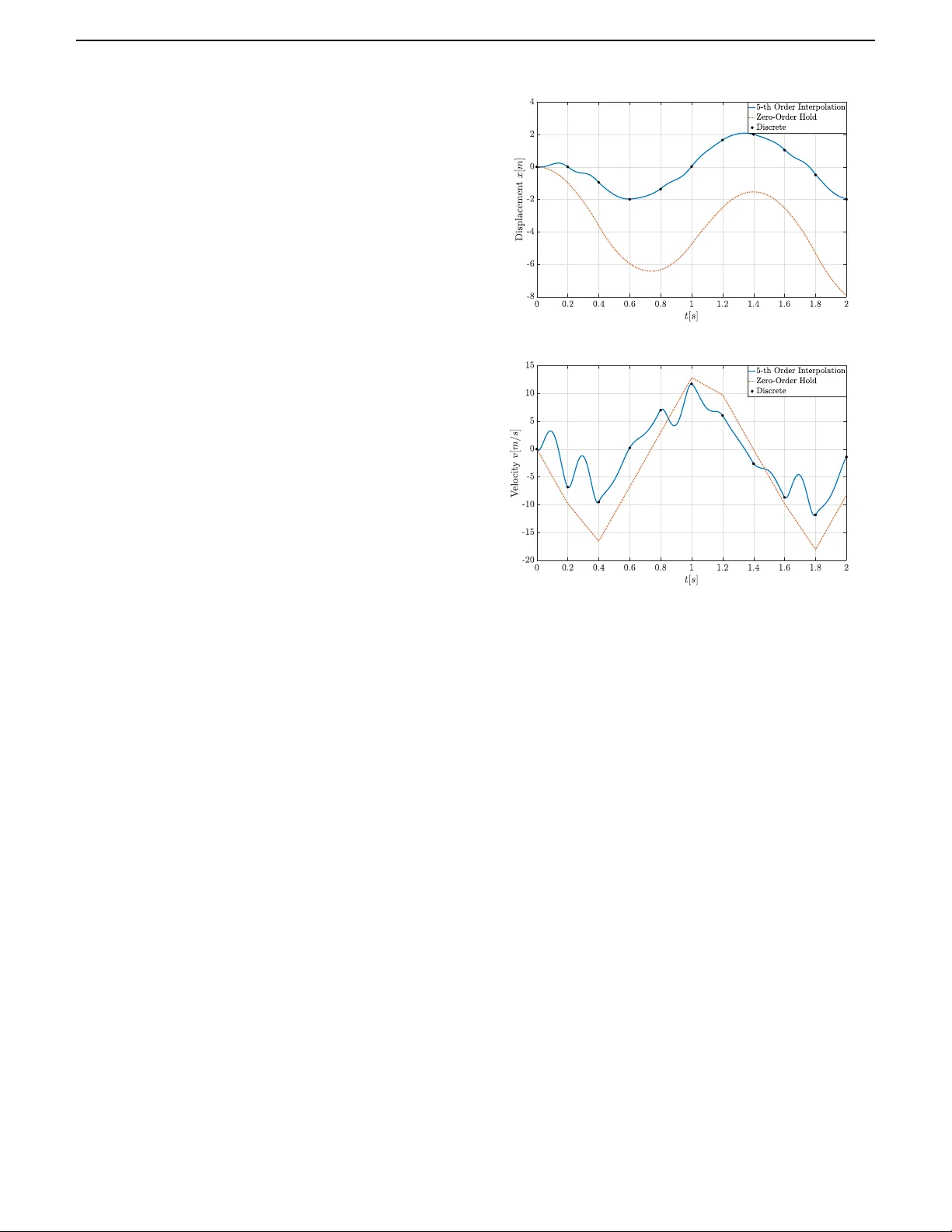
IEEE TRANSACTIONS ON A UT OMA TIC CONTROL 1 Compar ison of Linear Systems Across Time Domains: Continuous-time vs . Discrete-time Ar min Pirastehzad Member , IEEE and Bar t Besselink Senior Member , IEEE Abstract — W e develop a f ormal frame work f or the behav- ioral comparison of linear systems across different time domains. We accomplish this by introducing the notion of system interpolation, which determines whether the input- state trajectories of a continuous-time system can be re- alized as piecewise polynomial interpolations of the input- state trajectories of a discrete-time system. In this con- text, a piecewise pol ynomial interpolation of a discrete-time signal is characterized as a contin uous-time function that coincides with the discrete-time signal at given sampling instants and can be realiz ed as a polynomial of a prescribed degree over intervals between these instants. By represent- ing piecewise polynomial functions as linear combinations of shifted Legendre polynomials, we characterize system interpolation as a subspace inclusion that is completely in terms of system parameters. This therefore allows for a computationally efficient comparison of the input-state be- havior of a continuous-time system with that of a discrete- time one. W e then e xploit this characterization to discretize a given continuous-time system into a discrete-time one. Lastly , given a control specification, we exploit system interpolation to synthesize contr ollers that ensure satisfac- tion at each given sampling instant, while they measure the extent of (possible) violation over intervals between these instants. Index T erms — System comparison, formal methods, tem- poral logic, simulation relation, hybrid systems. I . I N T R O D U C T I O N M ODERN engineering applications often necessitate mo- bilization of autonomous systems, which are designed to operate in (uncertain) en vironments without continuous human intervention. Particularly , these systems are deployed in safety-critical technologies ( e.g., self-driving vehicles [1]), mission-critical utilities ( e.g., power grids [2]), and medical- critical services ( e .g., healthcare robots [3]). These applications often require autonomous systems to perform in accordance with intricate specifications, such as those expressed in terms of temporal logic formulae [4]. For continuous-time systems, such intricate specifications are usually enforced by controllers that are synthesized ac- cording to a hierar chical procedure [5]. In particular, many control schemes (see, e.g ., [6]–[13]) split synthesis into 1) discr etization , where a simplified discrete-time model of the continuous-time system is obtained, 2) planning , through which a discrete control sequence is designed to enforce All authors are with the Ber noulli Institute for Mathematics, Com- puterScience and Ar tificial Intelligence, University of Groningen, 9700 AK Groningen, The Nether lands (email: a.pirastehzad@rug.nl; b .besselink@r ug.nl). the discrete-time model to fulfill the specification, and 3) execution , which inv olves the synthesis of a continuous-time control that enforces the state trajectories of the original system to remain sufficiently close to the planned discrete- time trajectories. Since these hierarchical schemes enforce the continuous- time state trajectories to remain sufficiently close to inter- polations of the planned discrete-time state trajectories, they usually guarantee the specification only at certain instances of time rather than at all times. In fact, such schemes are inconclusiv e on how controlled continuous-time trajectories behav e with respect to the specification in between discrete time instances, i.e., it is not clear to what extent the con- trolled continuous-time trajectories satisfy/violate the spec- ification between these instances. Measuring the extent of satisfaction/violation of a specification ov er intervals between instances necessitates a metric that rigorously compares the behavioral similarity of the controlled continuous-time and the planned discrete-time trajectories. This paper proposes such metric by developing a formal framework for comparison of the input-state behavior of linear systems from continuous- time and discrete-time domains. This framew ork is then uti- lized for control synthesis to 1) ensure that the controlled continuous-time trajectories adhere to the specification at time instances that correspond to the planned discrete-time trajectories, and 2) measure the extent to which they may violate the specification in between these instances. A. Related W orks Behavioral similarity of dynamical systems has been con- sidered from a variety of perspectives. Inspired by concur - rency theory , the notion of (bi)simulation [14]–[16] utilizes the formalism of labeled transition systems to determine the ability of a system to reproduce the input-output behavior of another . The notion of (bi)simulation is further specialized to continuous-time systems in [17], where it is formulated as a modified disturbance decoupling problem and characterized al- gebraically . Generalization of (bi)simulation to control systems gav e rise to the notion of alternating (bi)simulation [18] which determines equiv alence of the controlled input-output behavior of two systems. The notion of (bi)simulation and its alternating version are further utilized for specification verification and control synthesis in [19]. As (bi)simulation fails to compare systems with similar (but not identical) input-output behaviors, the notion of approx- imate (bi)simulation was proposed in [20]–[23] to quantify 2 IEEE TRANSACTIONS ON AUT OMA TIC CONTROL behavioral closeness , and was later specialized to verification and synthesis in [24]–[27]. Howe ver , because approximate (bi)simulation relies on the L ∞ signal norm to measure behavioral closeness, it is not compatible with many ana- lytic/synthetic tools in control theory , which often employ the L 2 signal norm. T o address this limitation, the notion of ( γ , δ ) - similarity was proposed in [28], [29], which makes use of the L 2 signal norm to measure this closeness. While all the notions mentioned abov e provide a formal methodology for system comparison, they share the limitation that they only compare systems within a single time domain, i.e., they either compare continuous-time systems or discrete- time ones. Even in the case of hybrid systems, the notion of (bi)simulation (and its approximate variants) compares the continuous-time dynamics associated with each discrete mode in isolation, i.e., it compares the continuous-time dynamics for fixed discrete modes (see, e.g ., [19], [23]). Many hierarchical schemes for temporal logic control ( e.g., [6], [30]–[34]), howe ver , in volve an implicit comparison of the external behavior of a continuous-time system with that of its discrete-time model, as they aim to provide guarantees on the continuous-time system according to strategies planned for its discrete-time model. Ho wev er , such comparison highly depends on the specification, as the behavioral similarity of the continuous-time system and its discrete-time model is measured with respect to a given specification. In fact, none of these schemes provide a ‘context-independent’ formal methodology for comparison of the behavioral similarity of a continuous-time system and its discrete-time model. A context-independent comparison of continuous-time sys- tems and their discrete-time models is crucial, as many con- trol problems can be ef ficiently addressed in discrete time, e.g ., control for temporal logic specification [30], [35] and optimization-based approaches such as model predictive con- trol (MPC) [36]. Despite this importance, only a few method- ologies for such comparison have been proposed. Exploiting functional transformations to conv ert signals from one time domain to another , the notion of (alternating) F − 1 -simulation [13] determines whether a system is able to produce a trans- formation of the input-output behavior of another system, i.e., it determines whether the behavior of one system can be transformed into that of another . The notion of (alternating) F − 1 -simulation can be formulated within the framew ork of (alternating) simulation. For finite-state systems, such formu- lation allo ws for the adoption of fixed point theorems (see, e.g ., [19, Theorem 5.6]) to obtain a computationally efficient characterization of (alternating) F − 1 -simulation. For infinite- state systems, ho wev er, characterization of (alternating) F − 1 - simulation is computationally challenging. In fact, comparison of such systems according to (alternating) F − 1 -simulation requires state abstraction, which becomes computationally intractable as the system dimension grows. The goal of this paper is therefore to de velop a formal framew ork for ef ficiently comparing the input-state behavior of (infinite-state) linear systems across different time domains, namely the continuous and discrete one. B. Contributions First, we introduce the notion of system interpolation , which determines whether the input-state trajectories of a continuous- time system can be realized as piecewise polynomial interpo- lations of the input-state trajectories of a discrete-time system. Specifically , for a given sampling time and a prescribed polynomial degree, we identify a continuous-time system as an interpolator of a discrete-time one if, for any discrete input sequence to the discrete-time system, there exists a piecewise polynomial interpolation of this sequence subject to which the continuous-time system admits a state trajectory which is also a piecewise polynomial interpolation of the corresponding state trajectory of the discrete-time system. Here, we identify a piece wise polynomial interpolation of a discrete-time signal as a continuous-time function such that 1) at each sampling in- stant, the continuous-time function coincides with the discrete- time signal and 2) over each interval between two consecutiv e instants, the continuous-time function is represented by a polynomial of the prescribed degree. Second, we obtain an algebraic characterization of sys- tem interpolation that solely depends on parameters of the continuous-time and discrete-time systems. T o this end, we demonstrate that system interpolation can be inv estigated by considering discrete-time input-state trajectories over a single (discrete) time step, i.e., in order to inspect system interpolation, it suffices to check whether the continuous-time system can generate piecewise polynomial interpolations of discrete-time input-state trajectories over a single interval. W e accordingly characterize these piece wise polynomial interpo- lations as linear combinations of the so-called shifted Leg endre polynomials (see, e.g., [37], [38]). This then enables the char- acterization of system interpolation as a subspace inclusion that completely depends on parameters of the continuous-time and discrete-time systems. Such characterization is computa- tionally efficient since subspace inclusion can be formulated as a simple rank condition. Third, for a given input-state trajectory of the discrete-time system, we characterize the set of all interpolating inputs that enforce the continuous-time system to admit input-state trajectories that are piecewise polynomial interpolations of this discrete-time trajectory . Particularly , we use the characteriza- tion of system interpolation to construct each input in this set. Fourth, we use system interpolation to conduct discretiza- tion. Specifically , for a giv en sampling time and a prescribed polynomial degree, we discretize a gi ven continuous-time system into a discrete-time model in such a way that the former is an interpolator of the latter . W e accomplish this by making use of the algebraic characterization of system interpolation to characterize the existence of such discrete-time model in terms of a linear matrix equation, whose solution gi ves the parameters of this model. Fifth, we utilize system interpolation for control synthesis. Specifically , for a giv en specification, we synthesize con- trollers on the basis of a discrete-time model of the continuous- time system (obtained via discretization using system inter- polation) to 1) ensure that the controlled continuous-time trajectories adhere to the specification at each sampling instant ARMIN PIRASTEHZAD AND BART BESSELINK: COMP ARISON OF LINEAR SYSTEMS A CROSS TIME DOMAINS 3 and 2) give a measure of the extent to which these trajectories may violate the specification over intervals between consecu- tiv e sampling instances. In particular , by measuring (possible) specification violation in terms of the sampling time and the prescribed polynomial degree (of interpolation), we show how the extent of specification violation varies with respect to the sampling time and the polynomial degree. The rest of this paper is organized as follo ws. The problem statement is giv en in Section II. In Section III, we briefly revie w the basic properties of the shifted Legendre polyno- mials, based upon which the main results of the paper are built. W e then introduce and characterize the notion of system interpolation in Section IV. W e accordingly use this characteri- zation to conduct discretization in Section V. Subsequently , we utilize system interpolation for control synthesis in Section VI. W e further demonstrate our results in a numerical example in Section VII and finally conclude the paper by Section VIII. C . Notation The mathematical notation adopted in this paper is largely standard. Nevertheless, for clarity , we briefly revie w the gen- eral conv entions. Sets: W e respecti vely denote the set of real numbers and integers by R and Z , while we use R > 0 and Z > 0 to respec- tiv ely indicate the set of positiv e real numbers and integers. For real numbers t 1 ≤ t 2 , we denote the closed real interval { t ∈ R | t 1 ≤ t ≤ t 2 } by [ t 1 , t 2 ] . For integers k 1 ≤ k 2 , on the other hand, we use J k 1 , k 2 K to denote the closed integer interval { k ∈ Z | k 1 ≤ k ≤ k 2 } . W e utilize R n to denote the set of real vectors with n components, and write R n × m for the set of real n × m matrices. Then, we denote the image of a matrix M ∈ R n × m by Im M and define it as Im M = { y ∈ R n |∃ x ∈ R m : M x = y } . Operators: W e define the operator col( · , · ) such that col( x 1 , x 2 ) = ( x ⊤ 1 , x ⊤ 2 ) ⊤ , for any vectors x 1 ∈ R n 1 and x 2 ∈ R n 2 . The Euclidean norm of a vector x ∈ R n is defined as | x | = ( x ⊤ x ) 1 2 . Then, for a positiv e (semi-)definite matrix M ∈ R n × m , we define the weighted Euclidean (semi-)norm as | x | M = ( x ⊤ M x ) 1 2 . W e define the vectorization of a matrix M = [ M 1 M 2 · · · M m ] , with columns M 1 , M 2 , · · · , M m ∈ R n , as vec( M ) = col( M 1 , M 2 , · · · , M m ) . W e also utilize the symbol ⊗ to denote the Kronecker product. Indicating an identity matrix and a zero matrix of appropriate dimensions by I and 0 , respectiv ely , we define the Kronecker sum of square matrices N ∈ R n × n and M ∈ R m × m as N ⊕ M = N ⊗ I + I ⊗ M . Function Spaces and Operations: For real numbers τ 1 ≤ τ 2 , we define the space of n -dimensional vector -valued func- tions that are square-integrable over the interval [ τ 1 , τ 2 ] as L n 2 [ τ 1 , τ 2 ] = { u : [ τ 1 , τ 2 ] → R n | R τ 2 τ 1 | u ( t ) | 2 d t < ∞} , which is endowed with the norm ∥ u ∥ L n 2 [ τ 1 ,τ 2 ] = ( R τ 2 τ 1 | u ( t ) | 2 d t ) 1 2 . W e also define the space of n -dimensional v ector-v alued functions that are bounded ov er [ τ 1 , τ 2 ] as L n ∞ [ τ 1 , τ 2 ] = { u : [ τ 1 , τ 2 ] → R n | max t ∈ [ τ 1 ,τ 2 ] | u ( t ) | < ∞} , equipped with the norm ∥ u ∥ L n ∞ [ τ 1 ,τ 2 ] = max t ∈ [ τ 1 ,τ 2 ] | u ( t ) | . Giv en a set I , we define the restriction of a function u : I → R n to the subset I ′ ⊂ I as the function u | I ′ : I ′ → R n such that ∀ t ∈ I ′ : u | I ′ ( t ) = u ( t ) . Then, for a set F of functions f : I → R n , we define the restriction of F to I ′ as F | I ′ =  f | I ′   f ∈ F  . I I . P RO B L E M S T A T E M E N T For continuous-time systems, control synthesis for enforc- ing intricate specifications is usually split into (at least) the following consecuti ve tasks (see, e.g., [7]–[13]). 1) Discr etization : First, a simplified discr ete-time model of the continuous-time system is constructed, as demon- strated on the left side of Figure 1. Such a model is obtained either according to the occurrence of particular events , such as ev olution of state trajectories from one region of interest to another (see, e.g., [6]), or through discretization of system dynamics with respect to a sampling time (see, e.g., [11]). 2) Planning : Then, a discrete control sequence is designed to enforce the discrete-time model to fulfill the specifi- cation (see, e.g., [7], [8]). In fact, such control enforces the discrete-time model to admit a state trajectory that adheres to a discretized version of the original (contin- uous) specification, see the lower part of Figure 1. 3) Execution : Lastly , a continuous-time control is synthe- sized that enforces the original system to admit a state trajectory that is suf ficiently close to an interpolation of the planned discrete-time trajectory , see the middle part of Figure 1. Such control then enforces the system to (approximately) satisfy the specification, e.g., it may enforce the system to admit a trajectory whose samples adhere to the specification (see, e.g., [11], [13]). The prev alence of such hierarchical schemes stems from the fact that control synthesis for enforcing complex specifications is easier in the discrete-time than in the continuous-time. While these schemes guarantee that a discrete-time model of a continuous-time system satisfies a specification, they do not formally guarantee that the system itself fully satisfies the specification. This is a consequence of the fact that these schemes synthesize a controller that renders the continuous- time system to admit state trajectories that remain (sufficiently) close to interpolations of the state trajectories of its discrete- time model. In other words, despite enforcing the specification at certain instances ( e.g., sampled times), such a controller does not necessarily ensure satisfaction at all times. In fact, it is not clear how the controlled continuous-time system behaves with respect to the specification in between these instances, i.e., there is no measure of the extent to which the specification is satisfied/violated over intervals between the instances. Motiv ated by this, we dev elop a formal framework for comparison of the input-state beha vior of a continuous-time system with that of a discrete-time one. Specifically , we consider the continuous-time linear system Σ c : ˙ x c ( t ) = A c x c ( t ) + B c u c ( t ) , (1) with state x c ∈ R n and input u c ∈ R m . W e denote by x c ( t ; x 0 , u c ) the state solution, at time t , of (1) for initial condition x c (0) = x 0 and input u c . In correspondence to ( 1), we consider the discrete-time linear system Σ d : x d ( i + 1) = A d x d ( i ) + B d u d ( i ) , (2) 4 IEEE TRANSACTIONS ON AUT OMA TIC CONTROL Continuous-time System Continuous-time Control | = Continuous Specification Discrete-time System Discrete-time Control | = Discrete Specification Discretization Execution Planing Fig. 1 : Control synthesis for enforcing intricate specifications is usually split into 1) discretization of the continuous-time system into a simplified discrete-time model (see left side of the figure), 2) planning a trajectory (by designing a suitable discrete control sequence) for the discrete-time model that adheres to the specification (see the lower part of the figure), and 3) execution of a continuous-time control that utilizes an interpolation of the planned discrete-time trajectory to enforce the original system to (approximately) satisfy the specification (see the middle part of the figure). with state x d ∈ R n and u d ∈ R m . W e use notation similar to that of (1) to denote the state sequence of (2). Our goal is therefore to conceive a method that compares the input-state behavior of (1) with that of (2). W e will accomplish this by performing (piecewise) polynomial interpolation on the basis of Legendre polynomials, which are studied in the next section. I I I . L E G E N D R E P O L Y N O M I A L S W e briefly review basic properties of Legendre polynomials, which are extensiv ely utilized for polynomial interpolation as they form an orthogonal basis for the space of polynomials (for further details on orthogonality , see, e.g., [39]). Giv en any integer k ≥ 0 , let L k be the standard Legendre polynomial of degree k , defined as L k ( t ) = 1 2 k ⌊ k 2 ⌋ X i =0 ( − 1) i  k i   2 k − 2 i k  t k − 2 i , (3) where ⌊ k 2 ⌋ is the greatest integer less than or equal to k 2 (for an elaborate study of standard Legendre polynomials, see, e.g., [37], [40], [41]). Accordingly , for τ ∈ R > 0 , we define the shifted Legendre polynomial, of degree k , over the interval [0 , τ ] as L τ k ( t ) = L k  2 t τ − 1  . It then directly follows from the mutual orthogonality of standard Legendre polynomials ov er the interval [ − 1 , 1] (see, e.g ., [37, Section 2.2.2]) that for all integers k , l ≥ 0 , Z τ 0 L τ k ( t ) L τ l ( t )d t =    0 k  = l , τ 2 k + 1 k = l , (4) which indicates that shifted Legendre polynomials are linearly independent over the interval [0 , τ ] . Now , for any integer N ≥ 0 , we let P n N denote the space of all n -dimensional vector -valued polynomials up to degree N . W e thus conclude from the linear independence of shifted Legendre polynomials that P n N   [0 ,τ ] = ( N X k =0 α k L τ k   [0 ,τ ]      α 0 , α 1 , · · · , α N ∈ R n ) , (5) i.e., the restriction of any polynomial function (up to degree N ) to the interval [0 , τ ] can be written as a linear combination of the restriction of shifted Legendre polynomials (up to degree N ) to the interval [0 , τ ] . W e also note that P n N | [0 ,τ ] ⊂ L n 2 [0 , τ ] ∩ L n ∞ [0 , τ ] . Subsequently , we construct a quadrature rule that enables exact integration of polynomial functions over the interval [0 , τ ] . This requires a suitable choice of quadrature nodes and weights. For an integer N ≥ 1 , we choose the quadrature nodes t N , 0 < t N , 1 < . . . < t N ,N such that ∀ i ∈ { 0 , 1 , · · · , N } : L τ N ( t N ,i ) + L τ N +1 ( t N ,i ) = 0 , (6) i.e., t N , 0 , t N , 1 , . . . , t N ,N are chosen as the zeros of L τ N + L τ N +1 . W e emphasize that such quadrature nodes always exists as L τ N + L τ N +1 is a separable polynomial of degree N + 1 , i.e., it has N + 1 distinct roots (for more details, see [37, Section 2.2.3]). W e further note that t N , 0 = 0 and t N ,N < τ (see, e.g., [38, Section 2]). Corresponding to these nodes, we define the quadrature weights w N , 0 = τ ( N + 1) 2 , (7a) and w N ,i = 1 ( N + 1) 2 τ − t N ,i | L τ N ( t N ,i ) | 2 , (7b) for i = 1 , 2 , . . . , N . It now follows from Gauss-Radau quadra- ture (see, e.g., [37, Section 2.2.3]) that ∀ P ∈ P n 2 N : Z τ 0 P ( t )d t = N X i =0 P ( t N ,i ) w N ,i . (8) W e note that (8) enables computation of the L n 2 [0 , τ ] norm of polynomial functions in terms of their values at the quadra- ture nodes. More specifically , for any function P ∈ P n N | [0 ,τ ] , we employ (8) to obtain ∥ P ∥ L n 2 [0 ,τ ] = N X i =0 | P ( t N ,i ) | 2 w N ,i ! 1 2 . (9) W e further note that (8) facilitates the representation of a function P ∈ P n N | [0 ,τ ] in terms of its values at quadrature nodes. Giv en P ∈ P n N | [0 ,τ ] , it follows from (5) that there exist vector -valued coefficients α 0 , α 1 , · · · , α N ∈ R n such that ∀ t ∈ [0 , τ ] : P ( t ) = N X k =0 α k L τ k   [0 ,τ ] ( t ) . (10) Bearing in mind that P L τ k | [0 ,τ ] ∈ P n 2 N | [0 ,τ ] for all k = 0 , 1 , · · · , N , we immediately conclude from (4) that α k = 2 k + 1 τ Z τ 0 P ( t ) L τ k ( t )d t, ARMIN PIRASTEHZAD AND BART BESSELINK: COMP ARISON OF LINEAR SYSTEMS A CROSS TIME DOMAINS 5 which, as a consequence of (8), can be written as α k = 2 k + 1 τ N X i =0 P ( t N ,i ) L τ k ( t N ,i ) w N ,i . (11) Thus, after defining the function ϕ i : [0 , τ ] → R as ϕ i ( t ) = N X k =0 2 k + 1 τ  L τ k ( t N ,i ) w N ,i  L τ k ( t ) , (12) we substitute (11) into (10) to obtain ∀ t ∈ [0 , τ ] : P ( t ) = N X i =0 ϕ i ( t ) P ( t N ,i ) , (13) which suggests that P can be written in terms of its values at the quadrature nodes. More importantly , we may exploit (13) to obtain a closed-form expression of (12). T o accomplish this, we consider the scalar function L i ( t ) = N Y j =0 ,j  = i ( t − t N ,j ) , which is a polynomial, of degree N , whose roots include all quadrature nodes except for t N ,i . Bearing this in mind, we employ (13) to obtain ϕ i ( t ) = L i ( t ) L − 1 i ( t N ,i ) , from which we immediately conclude that ϕ i ( t ) = N Y j =0 ,j  = i t − t N ,j t N ,i − t N ,j . (14) W e note from the expression (14) that the function ϕ i is in fact a Lagr ange interpolating polynomial for the quadrature nodes (see, e.g., [42, Section 3.1]). W e further highlight that ϕ i ( t N ,j ) = ( 0 j  = i, 1 j = i, (15) for all i = 0 , 1 , . . . , N . Additionally , given the special struc- ture of (14), we may employ the product rule to obtain ˙ ϕ i ( t ) = N X l =0 ,l  = i   1 t N ,i − t N ,l N Y j =0 ,j  = i,l t − t N ,j t N ,i − t N ,j   . (16) T o recapitulate, we emphasize that any P ∈ P n N | [0 ,τ ] admits the representation (13), with ϕ i giv en by (14). W e note that the function ϕ i is independent of P as it is completely determined by the quadrature nodes. In the next section, we will extensiv ely use the representation (13), together with formulae (14) and (16), to compare continuous-time signals with discrete-time ones. I V . S Y S T E M I N T E R P O L A T I O N W e will use polynomial interpolation on the basis of shifted Legendre polynomials to propose a technique for comparison of the input-state behaviors of systems (1) and (2). For this purpose, we first interpolate discrete-time signals into continuous-time piecewise polynomial ones according to the following definition. Definition 1: For ℓ, p ∈ Z > 0 , let a discrete-time signal s d : J 0 , ℓ K → R p be giv en. For a sampling time τ ∈ R > 0 and an integer N ≥ 1 , a continuous-time signal s c : [0 , ℓτ ] → R p is said to be an N -th order interpolation of s d with respect to the sampling time τ if there exist polynomial functions P 0 , P 1 , · · · , P ℓ − 1 ∈ P p N | [0 ,τ ] such that for all i ∈ J 0 , ℓ − 1 K , we have that s c ( iτ ) = s d ( i ) , s c  ( i + 1) τ  = s d ( i + 1) (17a) and ∀ t ∈ [0 , τ ] : s c ( iτ + t ) = P i ( t ) . (17b) According to Definition 1, the continuous-time signal s c : [0 , ℓτ ] → R p is an N -th order interpolation of the discrete- time signal s d : J 0 , ℓ K → R p with respect to the sampling time τ if its v alue at any time iτ equals the value of s d at instance i , while its restriction to the interval [ iτ , ( i + 1) τ ] can be described by a polynomial in P p N | [0 ,τ ] . W e note that for N ≥ 2 , an N -th order interpolation of a discrete-time signal s d with respect to sampling time τ is not unique. Thus, we denote by I τ N ( s d ) the set of all N -th order interpolations of a given discrete-time signal s d : J 0 , ℓ K → R p with respect to the sampling time τ . Having defined piece wise polynomial interpolation of discrete-time signals, we now propose the following notion of comparison that determines whether a continuous-time system is able to generate an interpolation of the input-state behavior of a discrete-time system. Definition 2: For a sampling time τ ∈ R > 0 and an integer N ≥ 1 , a continuous-time system Σ c is said to be an N -th order interpolator of a discrete-time system Σ d with respect to the sampling time τ if for any integer ℓ ∈ Z > 0 , any initial condition x 0 ∈ R n , and any discrete-time input u d : J 0 , ℓ K → R m , there exists a continuous-time input u c ∈ I τ N ( u d ) such that x c ( · ; x 0 , u c )   [0 ,ℓτ ] ∈ I τ N  x d ( · ; x 0 , u d )   J 0 ,ℓ K  . (18) It follows from Definition 2 that when Σ c is an N -th order interpolator of Σ d with respect to the sampling time τ , for any input-state trajectory in Σ d , there exists an input-state trajectory in Σ c that is its N -th order interpolation with respect to the sampling time τ . In other words, Σ c is able to generate an N -th order interpolation of any input-state trajectory of Σ d with respect to the sampling time τ . W e now propose the following result which allows for the in vestigation of system interpolation on the basis of a single (discrete) time step, i.e., in order to inspect system interpolation, it is sufficient to consider a single interval [0 , τ ] . This will later facilitate an algebraic characterization of system interpolation. Pr oposition 1: F or a sampling time τ ∈ R > 0 and an integer N ≥ 1 , Σ c is an N -th order interpolator of Σ d with respect to the sampling time τ if and only if for any x 0 ∈ R n and any u d : J 0 , 1 K → R m , there exists u c ∈ I τ N ( u d ) such that x c ( · ; x 0 , u c )   [0 ,τ ] ∈ I τ N  x d ( · ; x 0 , u d )   J 0 , 1 K  . (19) Pr oof: T o show necessity , let ℓ = 1 , x 0 ∈ R n , and u d : J 0 , ℓ K → R m . As Σ c is an N -th order interpolator of Σ d with respect to the sampling time τ , it follows from Definition 2 that there exists u c ∈ I τ N ( u d ) such that (19) holds. 6 IEEE TRANSACTIONS ON AUT OMA TIC CONTROL T o show sufficiency , let ℓ ∈ Z > 0 , x 0 ∈ R n , and u d : J 0 , ℓ K → R m . For any integer 0 ≤ i ≤ ℓ − 1 , we define u i d : J 0 , 1 K → R m such that u i d (0) = u d ( i ) , u i d (1) = u d ( i + 1) . (20) W e then note from time-in variance of Σ d that x d  · ; x d ( i ; x 0 , u d ) , u i d    J 0 , 1 K = x d ( · ; x 0 , u d )   J i,i +1 K . (21) It then follows from the proposition statement that there exists u i c ∈ I τ N ( u i d ) such that x c  · ; x d ( i ; x 0 , u d ) , u i c    [0 ,τ ] ∈ I τ N  x d  · ; x d ( i ; x 0 , u d ) , u i d    J 0 , 1 K  . Then, bearing (21) in mind, we conclude from Definition 1 that there exists P i ∈ P n N | [0 ,τ ] such that x c  0; x d ( i ; x 0 , u d ) , u i c  = x d ( i ; x 0 , u d ) , x c  τ ; x d ( i ; x 0 , u d ) , u i c  = x d ( i + 1; x 0 , u d ) , (22a) and ∀ t ∈ [0 , τ ] : x c  t ; x d ( i ; x 0 , u d ) , u i c  = P i ( t ) . (22b) W e now construct the continuous-time input u c : [0 , ℓτ ] → R m such that for all integers 0 ≤ i ≤ ℓ − 1 , ∀ t ∈ [0 , τ ] : u c ( iτ + t ) = u i c ( t ) . (23) Recalling that u i c ∈ I τ N ( u i d ) , we utilize (23), together with (20), to conclude that u c ∈ I τ N ( u d ) . W e now show that (18) holds. For this purpose, we utilize induction to show that for all i ∈ J 0 , ℓ − 1 K , x c ( iτ ; x 0 , u c ) = x d ( i ; x 0 , u d ) , x c  ( i + 1) τ ; x 0 , u c  = x d ( i + 1; x 0 , u d ) , (24a) and ∀ t ∈ [0 , τ ] : x c ( iτ + t ; x 0 , u c ) = P i ( t ) . (24b) Bearing (23) in mind, we note from the uniqueness of the solution of (1) that ∀ t ∈ [0 , τ ] : x c ( t ; x 0 , u c ) = x c  t ; x 0 , u 0 c  = x c  t ; x d (0; x 0 , u d ) , u 0 c  , which, by (22), implies that (24) holds for i = 0 . W e now suppose that (24) holds for i = k − 1 , where 0 < k ≤ ℓ − 1 . It then follows from time-inv ariance of Σ c that for all t ∈ [0 , τ ] , x c ( k τ + t ; x 0 , u c ) = x c  t ; x c ( k τ ; x 0 , u c ) , u k c  , which, as a result of (24a), can be written as x c ( k τ + t ; x 0 , u c ) = x c  t ; x d ( k ; x 0 , u d ) , u k c  . It then follows from (22) that x c ( k τ ; x 0 , u c ) = x d ( k ; x 0 , u d ) , x c  ( k + 1) τ ; x 0 , u c  = x d ( k + 1; x 0 , u d ) , and ∀ t ∈ [0 , τ ] : x c ( k τ + t ; x 0 , u c ) = P k ( t ) , indicating that (24) holds for all i ∈ J 0 , ℓ − 1 K . This, by Definition 1, implies (18). W e no w utilize Proposition 1 to obtain an algebraic char- acterization of system interpolation. T o accomplish this, for a sampling time τ ∈ R > 0 , an integer N ≥ 1 , an initial condition x 0 ∈ R n , and a discrete-time input u d : J 0 , 1 K → R m , we suppose there exists a continuous-time input u c ∈ I τ N ( u d ) such that (19) holds. Considering that u c ∈ I τ N ( u d ) , we conclude from Defini- tion 1 that u c (0) = u d (0) , u c ( τ ) = u d (1) , (25) and that u c ∈ P n N | [0 ,τ ] . Accordingly , recalling that t N , 0 = 0 , we use (13) and (25) to write ∀ t ∈ [0 , τ ] : u c ( t ) = ϕ 0 ( t ) u d (0) + N X i =1 ϕ i ( t ) u c ( t N ,i ) , (26) where, for i = 0 , 1 , . . . , N , the function ϕ i is defined as in (14) and is therefore independent from u d . W e accordingly define the vector Φ =      ϕ 1 ( τ ) ϕ 2 ( τ ) . . . ϕ N ( τ )      (27) and the matrix U =  u c ( t N , 1 ) u c ( t N , 2 ) · · · u c ( t N ,N )  , (28) which, together with (26), allows us to write (25) as U Φ = u d (1) − ϕ 0 ( τ ) u d (0) . (29) W e now consider x c ( · ; x 0 , u c ) and utilize (19) to conclude from Definition 1 that x c (0; x 0 , u c ) = x 0 , x c ( τ ; x 0 , u c ) = x d (1; x 0 , u d ) , (30) and that x c ( · ; x 0 , u c ) | [0 ,τ ] ∈ P n N | [0 ,τ ] . This, using again (13), implies that for all t ∈ [0 , τ ] , x c ( t ; x 0 , u c ) = ϕ 0 ( t ) x 0 + N X i =1 ϕ i ( t ) x c ( t N ,i ; x 0 , u c ) . (31) Moreov er, for i = 1 , 2 , . . . , N , we define X i = x c ( t N ,i ; x 0 , u c ) (32) and construct the matrix X =  X 1 X 2 · · · X N  , (33) accordingly . W e then exploit (31) to write (30) as X Φ = x d (1; x 0 , u d ) − ϕ 0 ( τ ) x 0 , (34) where Φ is defined as in (27). Furthermore, after dif ferentiating (31) with respect to t , we substitute t = t N ,j and conclude from (1) that N X i =1 ˙ ϕ i ( t N ,j ) x c ( t N ,i ; x 0 , u c ) = A c x c ( t N ,j ; x 0 , u c ) (35) + B c u c ( t N ,j ) − ˙ ϕ 0 ( t N ,j ) x 0 , ARMIN PIRASTEHZAD AND BART BESSELINK: COMP ARISON OF LINEAR SYSTEMS A CROSS TIME DOMAINS 7 for all j = 0 , 1 , · · · , N . W e recall that the deriv ativ e ˙ ϕ i ( t ) is computed by (16). Subsequently , after defining the vector ψ j =      ˙ ϕ 1 ( t N ,j ) ˙ ϕ 2 ( t N ,j ) . . . ˙ ϕ N ( t N ,j )      , (36) for j = 0 , 1 , · · · , N , we construct the matrix Ψ =  ψ 1 ψ 2 · · · ψ N  . (37) W e write (35), ev aluated at j = 0 , as X ψ 0 =  A c − ˙ ϕ 0 (0) I n  x 0 + B c u d (0) , (38a) whereas we collect (35), ev aluated at j = 1 , 2 , . . . , N , into X Ψ = A c X + B c U − x 0 σ, (38b) where σ =  ˙ ϕ 0 ( t N , 1 ) · · · ˙ ϕ 0 ( t N ,N )  , (39) Finally , bearing in mind that x d (1; x 0 , u d ) = A d x 0 + B d u d (0) , we collect (29), (34), and (38) to obtain X ψ 0 =  A c − ˙ ϕ 0 (0) I n  x 0 + B c u d (0) , X Ψ − A c X − B c U = − x 0 σ, X Φ =  A d − ϕ 0 ( τ ) I n  x 0 + B d u d (0) , U Φ = u d (1) − ϕ 0 ( τ ) u d (0) . (40) The formulation (40) facilitates the following algebraic char- acterization of system interpolation, which is solely in terms of the parameters of Σ c and Σ d . Theor em 1: For a sampling time τ ∈ R > 0 and an integer N ≥ 1 , Σ c is an N -th order interpolator of Σ d with respect to the sampling time τ if and only if Im     A c − ˙ ϕ 0 (0) I B c 0 − σ ⊤ ⊗ I 0 0 A d − ϕ 0 ( τ ) I B d 0 0 − ϕ 0 ( τ ) I I     ⊂ Im     ψ ⊤ 0 ⊗ I 0 Ψ ⊤ ⊕ ( − A c ) − I ⊗ B c Φ ⊤ ⊗ I 0 0 Φ ⊤ ⊗ I     , (41) where ϕ 0 , Φ , ψ 0 , Ψ , and σ are respectiv ely given by (14), (27), (36), (37), and (39). Pr oof: T o show necessity , suppose Σ c is an N -th order interpolator of Σ d with respect to the sampling time τ . Let x 0 ∈ R n and u d : J 0 , 1 K → R m . It then follo ws from Proposition 1 that there exists u c ∈ I τ N ( u d ) such that (19) holds. W e then follow the procedure described above to conclude that (40) holds for matrices U and X respectiv ely defined as in (28) and (33). This, as a consequence of matrix vectorization, results in     ψ ⊤ 0 ⊗ I 0 Ψ ⊤ ⊕ ( − A c ) − I ⊗ B c Φ ⊤ ⊗ I 0 0 Φ ⊤ ⊗ I      v ec( X ) v ec( U )  =     A c − ˙ ϕ 0 (0) I B c 0 − σ ⊤ ⊗ I 0 0 A d − ϕ 0 ( τ ) I B d 0 0 − ϕ 0 ( τ ) I I       x 0 u d (0) u d (1)   . (42) As x 0 and u d are chosen arbitrarily , we conclude from (42) that (41) holds. T o show sufficienc y , suppose that (41) holds. Letting x 0 ∈ R n and u d : J 0 , 1 K → R m , we conclude from (41) that there exist matrices X ∈ R n × N and U ∈ R m × N such that (42) holds. W e will use this matrix U to construct u c : [0 , τ ] → R m such that u c ∈ I τ N ( u d ) and that (19) holds. W e then utilize Proposition 1 to conclude that Σ c is an N -th order interpolator of Σ d with respect to the sampling time τ . As the first step, we utilize matrix vectorization to equiv- alently write (42) as (40). W e let U 1 , U 2 , · · · , U N ∈ R m be the columns of U , i.e., U = [ U 1 U 2 · · · U N ] . W e then define u c : [0 , τ ] → R m such that ∀ t ∈ [0 , τ ] : u c ( t ) = ϕ 0 ( t ) u d (0) + N X i =1 ϕ i ( t ) U i , (43) which, as a consequence of (14), implies that u c ∈ P m N | [0 ,τ ] . W e note from (15) that u c ( t N , 0 ) = u d (0) and that ∀ i ∈ { 1 , . . . , N } : u c ( t N ,i ) = U i . W e further note from the last equation of (40) that u c ( τ ) = u d (1) . This, by Definition 1, indicates that u c ∈ I τ N ( u d ) . W e now show that (19) holds. For this purpose, we let X 1 , X 2 , · · · , X N ∈ R n be such that (33) holds. W e accord- ingly define ¯ x c : [0 , τ ] → R n such that ¯ x c ( t ) = ϕ 0 ( t ) x 0 + N X i =1 ϕ i ( t ) X i . which, as a result of (14), implies that ¯ x c ∈ P n N | [0 ,τ ] . Furthermore, it follows from (15) that ¯ x c ( t N , 0 ) = x 0 and that ∀ i ∈ { 1 , . . . , N } : ¯ x c ( t N ,i ) = X i , which, as a consequence of the third equation of (40), implies that ¯ x c ( τ ) = x d (1; x 0 , u d ) . This, by Definition 1, indicates that ¯ x c ∈ I τ N  x d ( · ; x 0 , u d )   J 0 , 1 K  . (44) It now remains to show that x c ( · ; x 0 , u c ) | [0 ,τ ] = ¯ x c . T o accomplish this, we first utilize the first and second equations of (40) to conclude that ∀ i ∈ { 0 , 1 , · · · , N } : ˙ ¯ x c ( t N ,i ) = A c ¯ x c ( t N ,i ) + B c u c ( t N ,i ) . Bearing in mind that ¯ x c , ˙ ¯ x c ∈ P n N | [0 ,τ ] and u c ∈ P m N | [0 ,τ ] , we utilize (9) to obtain Z τ 0 | ˙ ¯ x c ( t ) − A c ¯ x c ( t ) − B c u c ( t ) | 2 d t = N X i =0 | ˙ ¯ x c ( t N ,i ) − A c ¯ x c ( t N ,i ) − B c u c ( t N ,i ) | 2 w N ,i = 0 , which, in turn, implies that for all t ∈ [0 , τ ] , ˙ ¯ x c ( t ) = A c ¯ x c ( t ) + B c u c ( t ) . W e now define ˜ x c : [0 , τ ] → R n as ∀ t ∈ [0 , τ ] : ˜ x c ( t ) = x c ( t ; x 0 , u c ) − ¯ x c ( t ) . 8 IEEE TRANSACTIONS ON AUT OMA TIC CONTROL W e note from (44) that ˜ x c (0) = 0 . W e then utilize (1) to obtain ∀ t ∈ [0 , τ ] : ˙ ˜ x c ( t ) = A c ˜ x c ( t ) . (45) By recalling that ˜ x c (0) = 0 , we conclude from uniqueness of the solution of (45) that ∀ t ∈ [0 , τ ] : ˜ x c ( t ) = 0 , which indicates that x c ( · ; x 0 , u c ) | [0 ,τ ] = ¯ x c . It then follo ws from (44) that (19) holds. As x 0 ∈ R n and u d : J 0 , 1 K → R m are chosen arbitrarily , we conclude from Proposition 1 that Σ c is an N -th order interpolator of Σ d with respect to τ . Theorem 1 allo ws one to determine if Σ c is an N -th order interpolator of Σ d with respect to the sampling time τ by simply checking the subspace inclusion (41), which is solely in terms of τ , N , and the parameters of Σ c and Σ d . This is computationally efficient as (41) can be equiv alently formulated as a rank condition. Having characterized system interpolation, we now suppose that Σ c is an N -th order interpolator of Σ d with respect to the sampling time τ . Giv en ℓ ∈ Z > 0 , x 0 ∈ R n , and u d : J 0 , ℓ K → R m , we employ Theorem 1 and Proposition 1 to characterize the set of all continuous-time inputs u c ∈ I τ N ( u d ) that establish (18). T o accomplish this, for any integer 0 ≤ i ≤ ℓ − 1 , we let X i ∈ R n × N and U i ∈ R m × N be such that     ψ ⊤ 0 ⊗ I 0 Ψ ⊤ ⊕ ( − A c ) − I ⊗ B c Φ ⊤ ⊗ I 0 0 Φ ⊤ ⊗ I      v ec( X i ) v ec( U i )  =     A c − ˙ ϕ 0 (0) I B c 0 − σ ⊤ ⊗ I 0 0 A d − ϕ 0 ( τ ) I B d 0 0 − ϕ 0 ( τ ) I I       x d ( i ; x 0 , u d ) u d ( i ) u d ( i + 1)   . (46) W e note from Theorem 1 that (46) is always consistent , i.e., there exist matrices X i and U i such that (46) holds. It is also worth noting that the matrices X i and U i are not necessarily unique. W e then partition U i as U i = [ U i 1 U i 2 · · · U i N ] and accordingly define u i c ∈ P m N | [0 ,τ ] such that ∀ t ∈ [0 , τ ] : u i c ( t ) = ϕ 0 ( t ) u d ( i ) + N X j =1 ϕ j ( t ) U i j . (47) Hence, we observe that the solutions of (46) induce a set U i c ( x 0 , u d ) = n u i c ∈ P m N   [0 ,τ ]    ∃ X i , U i s.t. (46)–(47) hold o , (48) based on which, we construct the set of continuous-time inputs U c ( x 0 , u d ) = n u c : [0 , ℓτ ] → R m   ∀ i ∈ J 0 , ℓ − 1 K , (49) ∃ u i c ∈ U i c ( x 0 , u d ) s.t. (23) holds o . W e note that since (46) is consistent for any choice of ℓ ∈ Z > 0 , x 0 ∈ R n , and u d : J 0 , ℓ K → R m , the set U c ( x 0 , u d ) is always non-empty . This observation is formally stated in the following lemma. Lemma 1: For a sampling time τ ∈ R > 0 and an integer N ≥ 1 , suppose Σ c is an N -th order interpolator of Σ d with respect to the sampling time τ . Then, for any ℓ ∈ Z > 0 , x 0 ∈ R n , and u d : J 0 , ℓ K → R m , the set of continuous-time inputs U c ( x 0 , u d ) , defined in (49), is non-empty . Pr oof: Let ℓ ∈ Z > 0 , x 0 ∈ R n , and u d : J 0 , ℓ K → R m . Since Σ c is an N -th order interpolator of Σ d with respect to τ , it follo ws from Theorem 1 that for any integer 0 ≤ i ≤ ℓ − 1 , there exist matrices X i ∈ R n × N and U i ∈ R m × N such that (46) holds. W e may therefore use this matrix U i to define u i c ∈ P m N | [0 ,τ ] as in (47). It thus follows from (48) that U i c ( x 0 , u d ) is non-empty for all 0 ≤ i ≤ ℓ − 1 , which, by (49), implies that U c ( x 0 , u d ) is non-empty . W e now exploit Lemma 1 to obtain the follo wing result, which shows that U c ( x 0 , u d ) is the set of all continuous-time inputs u c ∈ I τ N ( u d ) that establish (18). Theor em 2: For a sampling time τ ∈ R > 0 and an integer N ≥ 1 , suppose Σ c is an N -th order interpolator of Σ d with respect to the sampling time τ . Then, for any integer ℓ ∈ Z > 0 , any initial condition x 0 ∈ R n , and any discrete-time input u d : J 0 , ℓ K → R m , u c ∈ U c ( x 0 , u d ) ⇐ ⇒ u c ∈ I τ N ( u d ) s.t. (18) holds, (50) where U c ( x 0 , u d ) is defined as in (49). Pr oof: Let ℓ ∈ Z > 0 , x 0 ∈ R n , and u d : J 0 , ℓ K → R m . Since Σ c is an N -th order interpolator of Σ d with respect to τ , it follows from Lemma 1 that U c ( x 0 , u d ) is non-empty . W e first let u c ∈ U c ( x 0 , u d ) and show that u c ∈ I τ N ( u d ) and that (18) holds. T o do so, for any integer 0 ≤ i ≤ ℓ − 1 , we define u i d : J 0 , 1 K → R m according to (20). W e also let u i c : [0 , τ ] → R m be such that (23) holds. It then follows from the definition of U c ( x 0 , u d ) in (48) and (49) that there exist X i ∈ R n × N and U i ∈ R m × N such that (46) and (47) hold. Bearing (20) in mind, we follow the sufficiency part of the proof of Theorem 1 to conclude that u i c ∈ I τ N ( u i d ) . Furthermore, after partitioning X i as X i = [ X i 1 X i 2 · · · X i N ] , the procedure described in the proof of Theorem 1 gives x c  · ; x d ( i ; x 0 , u d ) , u i c    [0 ,τ ] ∈ I τ N  x d  · ; x d ( i ; x 0 , u d ) , u i d    J 0 , 1 K  . Additionally , we hav e that x c  0; x d ( i ; x 0 , u d ) , u i c    [0 ,τ ] = x d ( i ; x 0 , u d ) , (51a) and that, at the quadrature nodes, x c  t N ,j ; x d ( i ; x 0 , u d ) , u i c    [0 ,τ ] = X i j , (51b) for all j = 1 , 2 , . . . , N . W e then recall (21) and follow the sufficiency part of the proof of Proposition 1 to conclude that u c ∈ I τ N ( u d ) and that (18) holds. Importantly , it also follows from the proof of Proposition 1 that for all integers 0 ≤ i ≤ ℓ − 1 , we have that for all t ∈ [0 , τ ] , x c ( iτ + t ; x 0 , u c ) = ϕ 0 ( t ) x d ( i ; x 0 , u d ) + N X j =1 ϕ j ( t ) X i j . (52) Moreov er, it follows from (51) that x c ( iτ ; x 0 , u c ) = x d ( i ; x 0 , u d ) , (53a) and that ∀ j ∈ { 1 , 2 , . . . , N } : x c ( iτ + t N ,j ; x 0 , u c ) = X i j . (53b) ARMIN PIRASTEHZAD AND BART BESSELINK: COMP ARISON OF LINEAR SYSTEMS A CROSS TIME DOMAINS 9 W e now let u c ∈ I τ N ( u d ) be such that (18) holds, and we show that u c ∈ U c ( x 0 , u d ) . T o accomplish this, for any integer 0 ≤ i ≤ ℓ − 1 , we define u i d : J 0 , 1 K → R m and u i c : [0 , τ ] → R m such that (20) and (23) hold. Bearing (21) in mind, we conclude from u c ∈ I τ N ( u d ) and (18) that u i c ∈ I τ N ( u i d ) and that x c  · ; x d ( i ; x 0 , u d ) , u i c    [0 ,τ ] ∈ I τ N  x d  · ; x d ( i ; x 0 , u d ) , u i d    J 0 , 1 K  . Now , for j = 1 , 2 , . . . , N , we define U i j = u i c ( t N ,j ) , X i j = x c ( iτ + t N ,j ; x 0 , u c ) , and accordingly construct the matrices U i =  U i 1 , U i 2 , · · · , U i N  , X i =  X i 1 , X i 2 , · · · , X i N  . (54) W e then conclude from u i c ∈ I τ N ( u i d ) that (47) holds. More- ov er, we follow the necessity part of the proof of Theorem 1 to conclude that (46) holds. As a consequence, for all 0 ≤ i ≤ ℓ − 1 , there exist matrices U i and X i such that (46) and (47) hold, which, together with (49) and (48), implies that u c ∈ U c ( x 0 , u d ) . According to Theorem 2, for giv en ℓ ∈ Z > 0 , x 0 ∈ R n , and u d : J 0 , ℓ K → R m , U c ( x 0 , u d ) is the set of all continuous-time inputs u c ∈ I τ N ( u d ) that establish (18). This is crucial as it practically gives a step-by-step procedure for the construction of such u c . In fact, gi ven any u d : J 0 , ℓ K → R m , one may follow the first part of the proof of Theorem 2 to construct a u c ∈ I τ N ( u d ) that establishes ( 18). This becomes essential in control synthesis for a continuous-time system on the basis of its discrete-time model (see Section VI). V . D I S C R E T I Z A T I O N B Y S Y S T E M I N T E R P O L A T I O N W e now exploit system interpolation to conduct discretiza- tion. More specifically , giv en a continuous-time system (1), for a sampling time τ ∈ R > 0 and an integer N ≥ 1 , we construct a discrete-time system (2) in such a way that (1) is an N -th order interpolator of (2) with respect to the sampling time τ . For this purpose, we make use of Theorem 1 and seek matrices A d and B d such that (41) holds. W e therefore consider the subspace inclusion (41), where matrices A d and B d are now regarded as unknowns . It follows from (41) that there exists a matrix M ∈ R ( nN + mN ) × ( n +2 m ) such that     ψ ⊤ 0 ⊗ I 0 Ψ ⊤ ⊕ ( − A c ) − I ⊗ B c Φ ⊤ ⊗ I 0 0 Φ ⊤ ⊗ I     M =     A c − ˙ ϕ 0 (0) I B c 0 − σ ⊤ ⊗ I 0 0 A d − ϕ 0 ( τ ) I B d 0 0 − ϕ 0 ( τ ) I I     , which can be written as Q τ N ( A c , B c ) M = R τ N ( A c , B c ) + T 1  A d B d  T 2 , (55) where Q τ N ( A c , B c ) =     ψ ⊤ 0 ⊗ I 0 Ψ ⊤ ⊕ ( − A c ) − I ⊗ B c Φ ⊤ ⊗ I 0 0 Φ ⊤ ⊗ I     , R τ N ( A c , B c ) =     A c − ˙ ϕ 0 (0) I B c 0 − σ ⊤ ⊗ I 0 0 − ϕ 0 ( τ ) I 0 0 0 − ϕ 0 ( τ ) I I     , (56a) and T 1 =     0 0 I 0     , T 2 =  I 0 0 0 I 0  . (56b) W e emphasize that matrices Q τ N ( A c , B c ) and R τ N ( A c , B c ) solely depend on the quadrature nodes (which are determined by the sampling time τ and the polynomial degree N ) and the known matrices A c and B c . W e also highlight that the representation (55) is linear in terms of the unknown matrices M , A d , and B d . This representation thus enables the following result, which characterizes the existence of matrices A d and B d as the solvability of a linear equation that is completely in terms of the quadrature nodes and the system parameters A c and B c . Theor em 3: Gi ven a continuous-time system (1), for a sam- pling time τ ∈ R > 0 and an integer N ≥ 1 , there exist matrices A d and B d such that (1) is an N -th order interpolator of (2) with respect to the sampling time τ if and only if there exist vectors v 1 and v 2 such that  I ⊗ Q τ N ( A c , B c ) − T ⊤ 2 ⊗ T 1   v 1 v 2  = vec  R τ N ( A c , B c )  . (57) Pr oof: T o show necessity , we suppose that there exist A d and B d such that (1) is an N -th order interpolator of (2) with respect to the sampling time τ . It then follows from Theorem 1 that (41) holds. This, as discussed abov e, implies the existence of a matrix M such that (55) holds. Then, vectorization of (55) leads to (57) with v 1 = vec( M ) , v 2 = vec   A d B d   . (58) T o prove sufficienc y , we suppose that there exist matrices v 1 and v 2 such that (57) holds. W e then let matrices M , A d , and B d be such that (58) hold. W e then e xploit matrix vectorization to conclude (55). This, together with (56), implies (41). It then follows from Theorem 1 that (1) is an N -th order interpolator of (2) with respect to the sampling time τ . Theorem 3 characterizes existence of the discrete-system (2) as solvability of the linear equation (57), whose solution gives the parameters of (2), i.e., matrices A d and B d . In the next section, we make use of the discrete-time system (2), obtained according to Theorem 3, to conduct control synthesis for the continuous-time system (1). V I . S Y S T E M I N T E R P O L A T I O N F O R C O N T R O L S Y N T H E S I S As discussed earlier , hierarchical control schemes that split synthesis into discretization, planning, and execution do not formally guarantee that the continuous-time system fully com- plies with a specification, as they only guarantee that its state trajectories remain sufficiently close to an interpolation of the planned trajectory (which satisfies the specification only at particular time instances rather than all times). In fact, such schemes often do not provide any measure of the extent to which the specification is satisfied/violated in between these instances. Motiv ated by this, we utilize system interpolation in control synthesis to 1) ensure that the controlled continuous- time trajectories adhere to the specification at each sampled 10 IEEE TRANSACTIONS ON AUT OMA TIC CONTROL time and 2) measure to what extent they may violate the specification in between the sampled times. W e therefore consider the continuous-time system (1) and use Theorem 3 to construct its discrete-time model ( 2) for some sampling time τ ∈ R > 0 and integer N ≥ 1 . W e thus emphasize that (1) is an N -th order interpolator of (2) with respect to τ . Giv en a specification S , for an initial condition x 0 ∈ R n , suppose that (for some ℓ ∈ Z > 0 ) the control sequence u d : J 0 , ℓ K → R m is already designed in such a way that x d ( · ; x 0 , u d ) adheres to the specification S . This induces a path of regions Π ℓ := π 0 π 1 · · · π ℓ , (59) where the r egions of inter est π 0 , π 1 , · · · , π ℓ ⊂ R n , which are dictated by the specification S , are such that ∀ i ∈ J 0 , ℓ K : x d ( i ; x 0 , u d ) ∈ π i . (60) The path Π ℓ therefore accepts the specification S in the sense that the regions of interest π 0 , π 1 , · · · , π ℓ and the order according to which they appear conform to the specification S (for further details, see, e.g ., [6], [8], [43]). Remark 1: W e emphasize that we are not concerned with the design of the control sequence u d , as it depends on the specification S . In accordance to the expression of S , the control sequence u d can be designed by techniques such as dynamic programming [44], MPC [36], mixed integer linear/quadratic programming (MILP/MIQP) [35], [45], [46], and symbolic control [5], [43]. △ W e make use of the initial condition x 0 and the discrete-time input u d obtained abov e to construct the set of continuous- time inputs U c ( x 0 , u d ) as in (49). Since Σ c is an N -th order interpolator of Σ d with respect to τ . It follows from Theorem 2 that any u c ∈ U c ( x 0 , u d ) establishes (18). This, as a consequence of (60), implies that for all u c ∈ U c ( x 0 , u d ) , we have that ∀ i ∈ J 0 , ℓ K : x c ( iτ ; x 0 , u c ) ∈ π i , (61) i.e., the controlled trajectory x c ( · ; x 0 , u c ) satisfies the specifi- cation S at each sampled time t = iτ (for i = 0 , 1 , · · · , ℓ ). This therefore indicates that by choosing the continuous-time control input u c ∈ U c ( x 0 , u d ) , one ensures that the controlled continuous-time trajectories adhere to the specification at each sampled time. W e now employ (61) to measure the (possible) violation of S in between sampled times. T owards that end, we first define the distance of a point z ∗ ∈ R n from a region π ⊂ R n , denoted by d( z ∗ , π ) , as d( z ∗ , π ) = inf z ∈ π | z ∗ − z | . (62) W e accordingly define the Hausdorff distance [47] between two regions π , π ′ ⊂ R n , denoted by dH( π , π ′ ) , as dH( π , π ′ ) = max  sup z ∈ π d( z , π ′ ) , sup z ′ ∈ π ′ d( z ′ , π )  . (63) Then, for a point z ∗ ∈ R n and regions π , π ′ ⊂ R n , we observe that d( z ∗ , π ) ≤ d( z ∗ , π ′ ) + dH( π , π ′ ) , (64) which indicates that the distance d( z ∗ , π ) can be estimated in terms of the distance d( z ∗ , π ′ ) and the Hausdorff distance dH( π , π ′ ) (for further details, see, e.g., [47, Section 1.2.4]). Between two consecutiv e sampled times, we will use the estimation (64) to measure the (possible) violation of S . T aking any u c ∈ U c ( x 0 , u d ) , we note that (52) and (53) hold for all i ∈ J 0 , ℓ − 1 K and all t ∈ [0 , τ ] . Thus, for any j ∈ { i, i + 1 } , it follows from (61) that d  x c ( iτ + t ; x 0 , u c ) , π j  = inf z ∈ π j | x c ( iτ + t ; x 0 , u c ) − z | ≤   x c ( iτ + t ; x 0 , u c ) − x c ( j τ ; x 0 , u c )   =     Z iτ + t j τ ˙ x c ( ˆ t ; x 0 , u c )d ˆ t     ≤     Z iτ + t j τ | ˙ x c ( ˆ t ; x 0 , u c ) | d ˆ t     ≤ τ ∥ ˙ x c ( · ; x 0 , u c ) ∥ L n ∞ [ iτ , ( i +1) τ ] , which, as a consequence of (1), results in d  x c ( iτ + t ; x 0 , u c ) , π j  (65) ≤ τ ∥ A c x c ( · ; x 0 , u c ) + B u c ∥ L n ∞ [ iτ , ( i +1) τ ] . Considering that  A c x c ( · ; x 0 , u c ) + B u c    [ iτ , ( i +1) τ ] ∈ P n N   [ iτ , ( i +1) τ ] , we now recall from [48, Theorem 4.9.6] that for any polyno- mial P ∈ P n N | [ iτ , ( i +1) τ ] , we have that ∥ P ∥ L n ∞ [ iτ , ( i +1) τ ] ≤ N  6 τ  1 2 ∥ P ∥ L 2 ∞ [ iτ , ( i +1) τ ] , which, together with (65), implies that d  x c ( iτ + t ; x 0 , u c ) , π j  ≤ N (6 τ ) 1 2 ∥ A c x c ( · ; x 0 , u c ) + B u c ∥ L n 2 [ iτ , ( i +1) τ ] = N (6 τ ) 1 2 Z ( i +1) τ iτ   A c x c ( ˆ t ; x 0 , u c ) + B u c ( ˆ t )   2 d ˆ t ! 1 2 . This, together with (23), giv es d  x c ( iτ + t ; x 0 , u c ) , π j  (66) ≤ N (6 τ ) 1 2  Z τ 0   A c x c ( iτ + ˆ t ; x 0 , u c ) + B c u i c ( ˆ t )   2 d ˆ t  1 2 . W e then note from (52) that x c ( iτ + ˆ t ; x 0 , u c )   [0 ,τ ] ∈ P n N   [0 ,τ ] . Furthermore, it follows from (53) that x c ( iτ ; x 0 , u c ) = x d ( i ; x 0 , u d ) , and that x c ( iτ + t N ,j ; x 0 , u c ) = X i j , ARMIN PIRASTEHZAD AND BART BESSELINK: COMP ARISON OF LINEAR SYSTEMS A CROSS TIME DOMAINS 11 for all j = 1 , 2 , . . . , N . This therefore enables the utilization of (9) to write (66) as d  x c ( iτ + t ; x 0 , u c ) , π j  (67) ≤ N (6 τ ) 1 2    A c x d ( i ; x 0 , u d ) + B c u d ( i )   2 w N , 0 + N X j =1   A c X i j + B c U i j   2 w N ,j  1 2 , which, after the substitution of (7), giv es d  x c ( iτ + t ; x 0 , u c ) , π j  (68) ≤ N (6 τ ) 1 2 N + 1   A c x d ( i ; x 0 , u d ) + B c u d ( i )   2 τ + N X j =1   A c X i j + B c U i j   2 τ − t N ,i | L τ N ( t N ,i ) | 2 ! 1 2 . T o obtain a compact representation of the bound, we define the matrix W τ N =       τ − t N, 1 | L τ N ( t N, 1 ) | 2 I 0 · · · 0 0 τ − t N, 2 | L τ N ( t N, 2 ) | 2 I · · · 0 . . . . . . . . . . . . 0 0 · · · τ − t N,N | L τ N ( t N,N ) | 2 I       , and accordingly construct the matrix ∆ τ N ( A c , B c ) =  I ⊗ A c I ⊗ B c  ⊤ W τ N  I ⊗ A c I ⊗ B c  . (69) It now follows from (68) that d  x c ( iτ + t ; x 0 ,u c ) , π j  ≤ 6 1 2 τ N N + 1   A c x d ( i ; x 0 , u d ) + B c u d ( i )   + (6 τ ) 1 2 N N + 1      v ec( X i ) v ec( U i )      ∆ τ N ( A c ,B c ) . (70) W e utilize (70) to obtain the follo wing result, which measures the distance of a state v alue in between two sampled times from a region π ⊂ R n . Theor em 4: Let Σ c be an N -th order interpolator of Σ d with respect to a sampling time τ . Giv en regions of interest π 0 , π 1 , · · · , π ℓ ⊂ R n and an initial condition x 0 ∈ R n , for some ℓ ∈ Z > 0 , let the control sequence u d : J 0 , ℓ K → R m be such that (60) holds. T ake any continuous-time control input u c ∈ U c ( x 0 , u d ) . For any integer 0 ≤ i ≤ ℓ − 1 , let the function u i c ∈ U i c ( x 0 , u d ) and the matrices U i ∈ R m × N and X i ∈ R n × N be such that (23), ( 46), and (47) hold. Then, giv en a region π ⊂ R n , for all t ∈ [0 , τ ] , we hav e that d  x c ( iτ + t ; x 0 ,u c ) , π  ≤ 6 1 2 τ N N + 1   A c x d ( i ; x 0 , u d ) + B c u d ( i )   + (6 τ ) 1 2 N N + 1      v ec( X i ) v ec( U i )      ∆ τ N ( A c ,B c ) (71) + min  dH  π i , π  , dH  π i +1 , π  , where ∆ τ N ( A c , B c ) is defined as in (69). Pr oof: Let i ∈ J 0 , ℓ K and t ∈ [0 , τ ] . Then, for j ∈ { i, i + 1 } , it follows from (64) that d  x c ( iτ + t ; x 0 , u c ) , π  ≤ d  x c ( iτ + t ; x 0 , u c ) , π j  + dH  π j , π  . which, as a result of (70), immediately giv es (71). Remark 2: Theorem 4 giv es an upper bound , on the dis- tance of state values (between two consecutiv e sampled times) from a gi ven region, that depends on the solutions of (46). More specifically , giv en an initial condition x 0 ∈ R n and a control sequence u d : J 0 , ℓ K → R m that establishes (60) (for some regions of interest π 0 , π 1 , · · · , π ℓ ⊂ R n ), for any region π ⊂ R n , it follows from Theorem 4 that any continuous-time control input u c ∈ U c ( x 0 , u d ) enforces (71), which depends on matrices X i and U i that satisfy (46). Considering that these matrices are not necessarily unique, (71) suggests that one may reduce the distance between x c ( iτ + t ; x 0 , u c ) and π by constructing u c on the basis of matrices X i and U i that are obtained by minimizing      v ec( X i ) v ec( U i )      ∆ τ N ( A c ,B c ) with respect to (46). W e note that such minimization prob- lem can be cast into quadratic optimization with equality constraints, which admits a closed-form solution. Thus, by solving this optimization problem for all 0 ≤ i ≤ ℓ − 1 and constructing u c accordingly , one enforces the state x c ( iτ + t ; x 0 , u c ) to remain as close as possible to the region π . △ Measuring the distance of a state v alue in between sampled times from a giv en region in the state-space, Theorem 4 gives a measure of the extent to which a controlled continuous- time trajectory may violate a given specification. W e further demonstrate this in the following examples. Example 1: W e consider a safety-critical control problem. Giv en a ‘safe’ region π ⊂ R n and an initial condition x 0 ∈ π , for some ℓ ∈ Z > 0 , let the control sequence u d : J 0 , ℓ K → R m be such that ∀ i ∈ J 0 , ℓ K : x d ( i ; x 0 , u d ) ∈ π , (72) i.e., subject to the control sequence u d , the discrete-time model Σ d admits a state trajectory that remains within the safe region ov er the time interval J 0 , ℓ K . W e note that such u d can be obtained using techniques such as dynamic pr ogramming [44] and set-invariance control [49]. W e observe that (72) is obtained from (60) by choosing π i = π for all i = 0 , 1 , . . . , ℓ . Thus, by taking any u c ∈ U c ( x 0 , u d ) , we conclude from Theorem 4 that for any integer 0 ≤ i ≤ ℓ − 1 , ∀ t ∈ [0 , τ ] : d  x c ( iτ + t ; x 0 , u c ) , π  (73) ≤ 6 1 2 τ N N + 1   A c x d ( i ; x 0 , u d ) + B c u d ( i )   + (6 τ ) 1 2 N N + 1      v ec( X i ) v ec( U i )      ∆ τ N ( A c ,B c ) , which giv es an upper bound on the distance between the state x c ( iτ + t ; x 0 , u c ) and the safe region π . Importantly , 12 IEEE TRANSACTIONS ON AUT OMA TIC CONTROL (73) indicates that the distance from x c ( iτ + t ; x 0 , u c ) to π decreases with respect to the sampling time τ . This basically means that for a sufficiently small τ , the state x c ( iτ + t ; x 0 , u c ) remains desirably close to the safe region π . As (73) holds for all 0 ≤ i ≤ ℓ − 1 , we conclude that for a sufficiently small τ , the controlled continuous-time trajectory remains desirably close to the safe region π over the time interval [0 , ℓτ ] . Example 2: W e now consider a signal temporal logic (STL) control problem. For a vector Γ ∈ R n and a scalar γ ∈ R , we define the predicate µ as µ ( x ) := ( T rue , if Γ ⊤ x + γ ≥ 0 , F alse , if Γ ⊤ x + γ < 0 , and consider the specification S = G [ t 1 ,t 2 ] µ, where 0 ≤ t 1 < t 2 (for further details on STL, see, e.g ., [50]). W e note that the formula S requires the predicate µ to always remain true over the time interval [ t 1 , t 2 ] . Giv en an initial condition x 0 ∈ R n , for some ℓ ∈ Z > 0 , let the control sequence u d : J 0 , ℓ K → R m be such that x d (0; x 0 , u d ) | = G J i 1 ,i 2 K µ, where i 1 , i 2 ∈ J 0 , ℓ K are such that i 1 τ ≤ t 1 < t 2 ≤ i 2 τ . This implies that ∀ i ∈ J i 1 , i 2 K : µ  x d ( i ; x 0 , u d )  = T rue , (74) which induces a path (59) such that ∀ i ∈ J i 1 , i 2 K : π i =  x d ( i ; x 0 , u d )  , and that (60) holds. Then, taking any u c ∈ U c ( x 0 , u d ) , for any i 1 ≤ i ≤ i 2 , we let π =  x d ( i ; x 0 , u d )  , and immediately conclude from Theorem 4 that (73) holds. W e now define the STL score (see, e.g., [45], [50]) of x c ( t ; x 0 , u c ) with respect to the predicate µ as ρ  x c ( t ; x 0 , u c )  = Γ ⊤ x c ( t ; x 0 , u c ) + γ . W e let i ∈ J 0 , ℓ K and ˆ t ∈ [0 , τ ] be such that t = iτ + ˆ t . Recalling that u c ∈ U c ( x 0 , u d ) , we use (50) to conclude (18), which implies that x c ( iτ ; x 0 , u c ) = x d ( i ; x 0 , u d ) . This then enables us to write ρ  x c ( t ; x 0 , u c )  = Γ ⊤  x c ( iτ + ˆ t ; x 0 , u c ) − x d ( i ; x 0 , u d )  + ρ  x d ( iτ ; x 0 , u d )  , which, together with ( 73) and (74), giv es    ρ  x c ( t ; x 0 , u c )  − ρ  x d ( iτ ; x 0 , u d )     ≤ | Γ | d  x c ( iτ + ˆ t ; x 0 , u c ) , π  (75) ≤ 6 1 2 τ N | Γ | N + 1   A c x d ( i ; x 0 , u d ) + B c u d ( i )   + (6 τ ) 1 2 N | Γ | N + 1      v ec( X i ) v ec( U i )      ∆ τ N ( A c ,B c ) . W e observe that for any i 1 ≤ i ≤ i 2 , (75) giv es an upper bound on the deviation from the discrete-time STL score with respect to the predicate µ . W e therefore emphasize that (75) gives a measure of the extent to which the continuous- time trajectory x c ( · ; x 0 , u d ) may violate S (between two consecutiv e sampled times). W e further note from (75) that for a sufficiently small sampling time τ , the continuous-time STL score ρ  x c ( t ; x 0 , u c )  becomes desirably close to its discrete-time counterpart ρ  x d ( iτ ; x 0 , u d )  . This indicates that by choosing the sampling time τ suf ficiently small, the extent of (possible) specification violation becomes desirably small. T o recapitulate, employing system interpolation for control synthesis enables us to measure to what extent a specification may be violated in between sampled times. In fact, giv en an initial condition x 0 and a control sequence u d that enforces a discrete-time model Σ d of a continuous-time system Σ c to fulfill a specification S , choosing any continuous-time control input u c ∈ U c ( x 0 , u d ) enables us to 1) ensure that the controlled state trajectory satisfies S at each sampled time (as indicated by (61)), and 2) measure to what extent this trajectory may violate S in between sampled time (as shown in Theorem 4). V I I . N U M E R I C A L S I M U L A T I O N W e consider temporal logic control of a robotic agent with double-inte grator dynamics. Subject to a control force F c , the robot Σ c experiences the velocity v and the displacement x . This is captured by the equation of motion ˙ x ( t ) = v ( t ) , ˙ v ( t ) = 1 m c F c ( t ) , where m c denotes the mass of the robot. W e suppose that the robot is initially at full rest, i.e., x (0) = 0 and v (0) = 0 . The objectiv e is to apply the control force F c such that the robot Σ c ev olves according to the STL formula S c = F [0 . 2 , 0 . 8]  x ( t ) ≤ − 2  ∧ F [1 , 1 . 4]  x ( t ) ≥ 2  ∧ F [1 . 6 , 2]  x ( t ) ≤ − 2  ∧ G [0 , 2]  v ( t ) ≤ 15 ∧ v ( t ) ≥ − 15  . Specifically , the formula S c requires that 1) the displacement x eventually becomes less that − 2 between 0 . 2 and 0 . 8 seconds; 2) the displacement x eventually surpasses 2 between 1 and 1 . 4 seconds; 3) the displacement x eventually drops below − 2 between 1 . 6 and 2 seconds; 4) the velocity v always remains between − 15m / s and 15m / s . W e will utilize system interpolation to determine the control force F c subject to which the robot Σ c fulfills these require- ments. T aking x c = col( x, v ) and u c = 1 m c F c , we immediately observe that Σ c is governed by the dynamics (1) with A c =  0 1 0 0  , B c =  0 1  . ARMIN PIRASTEHZAD AND BART BESSELINK: COMP ARISON OF LINEAR SYSTEMS A CROSS TIME DOMAINS 13 W e will therefore establish the objectiv e by synthesizing the continuous-time control u c such that x c (0; 0 , u c ) | = S c . (76) W e accomplish this by splitting the continuous-time control synthesis into the following steps. First, we discretize the continuous-time dynamics (1). After choosing the sampling time τ = 0 . 2s and the integer N = 5 , we conclude from Theorem 3 that there exist matrices A d and B d such that (1) is an N -th order interpolator of (2). W e then utilize Theorem 3 to obtain A d =  0 . 6990 0 . 1398 0 . 0000 0 . 6990  , B d =  0 . 0000 0 . 1398  . As the next step, we design a control sequence u d such that (2) satisfies the formula S c at sampled times. Discretizing S c with respect to the sampling time 0 . 2s , we obtain the (discrete- time) STL formula S d = F J 1 , 4 K  x d, 1 ( i ) ≤ − 2  ∧ F J 5 , 7 K  x d, 1 ( i ) ≥ 2  ∧ F J 8 , 10 K  x d, 1 ( i ) ≤ − 2  ∧ G J 0 , 10 K  x d, 2 ( i ) ≤ 15 ∧ x d, 2 ( i ) ≥ − 15  , where x d, 1 and x d, 2 respectiv ely denote the first and second components of x d , i.e., x d = col( x d, 1 , x d, 2 ) . W e then adopt the approach taken in [35] to encode the formula S d as mixed-inte ger linear constraints on the control sequence u d (for further details, see [35, Section IV .B] and [45, Section 5.2]). This then leads to a mixed-inte ger linear programming feasibility problem whose solution gives the control sequence u d : J 0 , 10 K → R such that x d (0; x 0 , u d ) | = S d . The mixed-integer linear program is solv ed using the opti- mization toolbox of MA TLAB R2022b . As the final step, we use the designed control sequence u d to construct the set of continuous-time inputs U c (0 , u d ) , as in (49). W e note that for τ = 0 . 2 and N = 5 , for any i ∈ J 0 , 9 K , the matrix equation (46) admits a unique solution. This, together with (48) and (49), indicates that the set U c (0 , u d ) is a singleton. W e thus conclude from Theorem 2 that there uniquely exists u c ∈ I 0 . 2 5 ( u d ) that establishes x c ( · ; x 0 , u c )   [0 , 2] ∈ I 0 . 2 5  x d ( · ; x 0 , u d )   J 0 , 10 K  . The displacement x and the velocity v of the robot Σ c are depicted in Figure 2 (indicated by solid lines), whereas the continuous-time control u c ∈ U c (0 , u d ) is depicted in Figure 3 (indicated by solid lines). It is clear from Figure 2 that the continuous-time control u c ∈ U c (0 , u d ) enforces the robot Σ c to evolv e in accordance with the STL formula S c , i.e., u c ∈ U c (0 , u d ) is such that (76) holds. Particularly , it can be observed from Figure 2a that the displacement x reaches − 2m at 0 . 6 and 2 . 0 seconds, whereas it surpasses 2m ov er the interval [1 . 2 , 1 . 4] . According to Figure 2b, on the other hand, the velocity v always remains between − 15m / s and 15m / s . T o show the efficac y of control synthesis using system interpolation, we hav e also depicted the displacement x and (a) Displacement x . (b) V elocity v . Fig. 2 : Subject to the continuous-time control u c ∈ U c (0 , u d ) (indicated by solid lines in Figure 3), the robot Σ c expe- riences a displacement and a velocity that comply with the requirements specified by the STL formula S c . By contrast, subject to a continuous-time control u c obtained by ZOH interpolation (indicated by dashed lines in Figure 3), neither the displacement of the robot nor its velocity adhere to the formula S c . the velocity v of the robot Σ c (indicated by dashed lines) in Figure 2, subject to a continuous-time control u c obtained as a zero-order hold (ZOH) interpolation of the control sequence u d (indicated by dashed lines in Figure 3). It is clear from Figure 2 that subject to such control, the robot does not fulfill the requirements specified by the formula S c . Particularly , in this case, the velocity surpasses − 15m / s (between 1 . 6 and 2 . 0 seconds), while the displacement x nev er reaches 2 (between 1 and 1 . 4 seconds). Remark 3: In this numerical example, the control u c ∈ U c ( x 0 , u d ) enforced the continuous-time system Σ c to fully satisfy the STL formula S c . In general, howe ver , choosing u c ∈ U c ( x 0 , u d ) does not guarantee the full satisfaction of an STL formula, but rather it only guarantees satisfaction at instances corresponding to the sampling time τ . Nev ertheless, such choice enables us to measure the extent of (possible) specification violation in between these instances by making use of (71). In fact, by choosing u c ∈ U c ( x 0 , u d ) , we guarantee that the div ergence of state values from regions of interest 14 IEEE TRANSACTIONS ON AUT OMA TIC CONTROL Fig. 3 : Subject to the continuous-time control u c ∈ U c (0 , u d ) (indicated by solid lines), the robot Σ c experiences a displace- ment x (Figure 2a) and a velocity v (Figure 2b) that adhere to the requirements specified by the formula S c . Howe ver , subject to a continuous-time control u c obtained by ZOH interpolation of the control sequence u d (indicated by dashed lines), the displacement x of the robot does not comply with formula S c . (which are dictated by the formula) always remain within the bound specified by (71). △ V I I I . C O N C L U S I O N In this paper , we dev eloped a formal framework for com- parison of systems across different time domains. W e accom- plished this by introducing the notion of system interpolation, which determines whether the input-state trajectories of a continuous-time system can be realized as piecewise poly- nomial interpolations of input-state trajectories of a discrete- time system. Here, we characterized piecewise polynomial interpolation of a discrete-time signal as a continuous-time function such that, at given sampling instants, it coincides with the discrete-time signal and that, ov er each interval between consecutive instants, it is represented by a polynomial of a prescribed degree. W e then showed that in order to in vestigate system interpolation, it suffices to check whether the continuous-time dynamics can generate piecewise polyno- mial interpolations of the discrete-time input-state trajectories ov er an interval that corresponds to a single (discrete) time step. Accordingly , by representing these piecewise polyno- mial interpolations as linear combinations of shifted Legendre polynomials (up to a prescribed degree), we characterized system interpolation as a subspace inclusion that is solely in terms of the parameters of the continuous-time and discrete- time systems. Such characterization is computationally effi- cient as it can be formulated as a simple rank condition. Afterwards, for a giv en discrete-time input-state trajectory , we characterized the class of all inputs that enforce the continuous-time system to admit input-state trajectories that are realized as piecewise polynomial interpolations of this discrete-time trajectory . Subsequently , we exploited system interpolation to discretize a gi ven continuous-time dynamics into a discrete-time one. Lastly , for a given specification, we employed system interpolation for control synthesis to ensure that the controlled continuous-time trajectories adhere to the specification at each sampling instants and to measure the extent of (possible) specification violation ov er intervals between these instances. For the future, we aim to employ the notion of system inter- polation to conduct (signal/linear) temporal logic control for continuous-time systems. Particularly , our goal is to combine system interpolation with temporal logic design techniques dev eloped for discrete-time systems to provide guarantees on continuous-time ones that interpolate them. [1] P . Koopman and M. W agner , “ Autonomous vehicle safety: An interdis- ciplinary challenge, ” IEEE Intelligent T ransportation Systems Magazine , vol. 9, no. 1, pp. 90–96, 2017. [2] A. W . dos Santos Serra, H. A. Oli veira, L. A. de Souza Ribeiro, J. G. de Matos, A. C. Oli veira, and O. R. Saavedra, “Mission-critical microgrids: Strategies for safe and reliable operations, ” Electric P ower Systems Resear ch , vol. 245, p. 111625, 2025. [3] M. T av akoli, J. Carriere, and A. T orabi, “Robotics, smart wearable technologies, and autonomous intelligent systems for healthcare during the covid-19 pandemic: An analysis of the state of the art and future vision, ” Advanced Intelligent Systems , vol. 2, no. 7, p. 2000071, 2020. [4] M. Fisher, An intr oduction to practical formal methods using temporal logic . John Wile y & Sons, 2011. [5] X. Y in, B. Gao, and X. Y u, “Formal synthesis of controllers for safety- critical autonomous systems: Dev elopments and challenges, ” Annual Reviews in Control , vol. 57, p. 100940, 2024. [6] M. Kloetzer and C. Belta, “ A fully automated framework for control of linear systems from temporal logic specifications, ” IEEE Tr ansactions on Automatic Contr ol , vol. 53, no. 1, pp. 287–297, 2008. [7] P .-J. Meyer and D. V . Dimarogonas, “Compositional abstraction refine- ment for control synthesis, ” Nonlinear Analysis: Hybrid Systems , vol. 27, pp. 437–451, 2018. [8] ——, “Hierarchical decomposition of ltl synthesis problem for nonlinear control systems, ” IEEE Tr ansactions on Automatic Control , vol. 64, no. 11, pp. 4676–4683, 2019. [9] K. Mallik, A.-K. Schmuck, S. Soudjani, and R. Majumdar, “Compo- sitional synthesis of finite-state abstractions, ” IEEE T ransactions on Automatic Control , vol. 64, no. 6, pp. 2629–2636, 2019. [10] M. Zamani, M. Mazo, M. Khaled, and A. Abate, “Symbolic abstrac- tions of networked control systems, ” IEEE T ransactions on Contr ol of Network Systems , vol. 5, no. 4, pp. 1622–1634, 2018. [11] G. Pola and M. D. Di Benedetto, “Control of cyber-ph ysical-systems with logic specifications: A formal methods approach, ” Annual Reviews in Contr ol , vol. 47, pp. 178–192, 2019. [12] M. Zamani, G. Pola, M. Mazo, and P . T abuada, “Symbolic models for nonlinear control systems without stability assumptions, ” IEEE T ransactions on A utomatic Contr ol , v ol. 57, no. 7, pp. 1804–1809, 2012. [13] M. Mazo Jr ., W . Compton, M. H. Cohen, and A. D. Ames, “ A contract theory for layered control architectures, ” arXiv pr eprint arXiv:2409.14902 , 2024. [14] G. Lafferriere, G. J. Pappas, and S. Sastry , “Hybrid systems with finite bisimulations, ” in International Hybrid Systems W orkshop . Springer , 1997, pp. 186–203. [15] G. J. Pappas, G. Lafferriere, and S. Sastry , “Hierarchically consistent control systems, ” IEEE T ransactions on A utomatic control , vol. 45, no. 6, pp. 1144–1160, 2000. [16] G. J. Pappas, “Bisimilar linear systems, ” Automatica , vol. 39, no. 12, pp. 2035–2047, 2003. [17] A. van der Schaft, “Equiv alence of dynamical systems by bisimulation, ” IEEE T ransactions on Automatic Control , vol. 49, no. 12, pp. 2160– 2172, 2004. [18] P . T abuada, “Controller synthesis for bisimulation equivalence, ” Systems & Contr ol Letters , vol. 57, no. 6, pp. 443–452, 2008. [19] ——, V erification and control of hybrid systems: a symbolic appr oach . Springer Science & Business Media, 2009. [20] A. Girard and G. J. Pappas, “ Approximate bisimulations for nonlinear dynamical systems, ” in Proceedings of the 44th IEEE Conference on Decision and Control . IEEE, 2005, pp. 684–689. ARMIN PIRASTEHZAD AND BART BESSELINK: COMP ARISON OF LINEAR SYSTEMS A CROSS TIME DOMAINS 15 [21] ——, “ Approximation metrics for discrete and continuous systems, ” IEEE T ransactions on Automatic Contr ol , vol. 52, no. 5, pp. 782–798, 2007. [22] ——, “ Approximate bisimulation relations for constrained linear sys- tems, ” Automatica , vol. 43, no. 8, pp. 1307–1317, 2007. [23] A. Girard, A. A. Julius, and G. J. Pappas, “ Approximate simulation relations for hybrid systems, ” Discr ete event dynamic systems , vol. 18, no. 2, pp. 163–179, 2008. [24] G. Fiore, E. de Santis, G. Pola, and M. D. Di Benedetto, “On approxi- mate predictability of metric systems, ” in Proceedings of the 6th IF AC Confer ence on Analysis and Design of Hybrid Systems , vol. 51, no. 16. Elsevier , 2018, pp. 169–174. [25] G. Pola and M. D. Di Benedetto, “ Approximate supervisory control of nonlinear systems with outputs, ” in Pr oceedings of the 56th IEEE Confer ence on Decision and Contr ol . IEEE, 2017, pp. 2991–2996. [26] G. Pola and P . T abuada, “Symbolic models for nonlinear control systems: Alternating approximate bisimulations, ” SIAM Journal on Control and Optimization , vol. 48, no. 2, pp. 719–733, 2009. [27] A. A. Julius, A. DInnocenzo, M. D. Di Benedetto, and G. J. Pappas, “ Approximate equivalence and synchronization of metric transition systems, ” Systems & Control Letters , vol. 58, no. 2, pp. 94–101, 2009. [28] A. Pirastehzad, A. van der Schaft, and B. Besselink, “Comparison of non-deterministic stable linear systems by (,)-similarity , ” IEEE T rans- actions on Automatic Contr ol , pp. 1–16, 2024. [29] ——, “Specification verification and controller synthesis using ( γ , δ )- similarity , ” in Proceedings of the 62nd IEEE Conference on Decision and Contr ol , 2023, pp. 1692–1697. [30] I. Papusha, J. Fu, U. T opcu, and R. M. Murray , “ Automata theory meets approximate dynamic programming: Optimal control with temporal logic constraints, ” in Proceedings of the 55th IEEE Conference on Decision and Control , 2016, pp. 434–440. [31] J. Liu and N. Ozay , “ Abstraction, discretization, and robustness in temporal logic control of dynamical systems, ” in Pr oceedings of the 17th international conference on Hybrid systems: computation and contr ol , 2014. [32] ——, “Finite abstractions with robustness margins for temporal logic- based control synthesis, ” Nonlinear Analysis: Hybrid Systems , vol. 22, pp. 1–15, 2016. [33] V . Kurtz and H. Lin, “T emporal logic motion planning with con vex optimization via graphs of con vex sets, ” IEEE T ransactions on Robotics , vol. 39, no. 5, pp. 3791–3804, 2023. [34] D. Sun, J. Chen, S. Mitra, and C. Fan, “Multi-agent motion planning from signal temporal logic specifications, ” IEEE Robotics and Automa- tion Letters , vol. 7, no. 2, pp. 3451–3458, 2022. [35] V . Raman, A. Donzé, M. Maasoumy , R. M. Murray , A. Sangiovanni- V incentelli, and S. A. Seshia, “Model predictive control with signal tem- poral logic specifications, ” in Proceedings of the 53r d IEEE Conference on Decision and Contr ol , 2014, pp. 81–87. [36] B. Kouv aritakis and M. Cannon, “Model predictiv e control, ” Switzer- land: Springer International Publishing , vol. 38, no. 13-56, p. 7, 2016. [37] C. Canuto, M. Y . Hussaini, A. Quarteroni, and T . A. Zang, Spectral Methods: Fundamentals in Single Domains . Springer Berlin Heidel- berg, 2006. [38] Z.-q. W ang and B.-y . Guo, “Legendre-gauss-radau collocation method for solving initial value problems of first order ordinary differential equations, ” Journal of Scientific Computing , vol. 52, no. 1, pp. 226– 255, 2012. [39] G. Szeg, Orthogonal polynomials , ser . Colloquium Publications. Amer- ican Mathematical Society , 1939, vol. 23. [40] B. Guo, Spectral methods and their applications . W orld Scientific, 1998. [41] J. Shen, T . T ang, and L.-L. W ang, Spectral methods: algorithms, analysis and applications . Springer Science & Business Media, 2011, vol. 41. [42] J. D. Faires and R. L. Burden, Numerical Analysis , 9th ed. Cengage Learning, 2010. [43] C. Belta, B. Y ordanov , and E. A. Gol, F ormal methods for discr ete-time dynamical systems . Springer, 2017. [44] D. Bertsekas, Dynamic pro gramming and optimal control: V olume I . Athena Scientific, 2012. [45] C. Belta and S. Sadraddini, “Formal methods for control synthesis: An optimization perspectiv e, ” Annual Review of Control, Robotics, and Autonomous Systems , vol. 2, no. 1, pp. 115–140, 2019. [46] E. M. W olff, U. T opcu, and R. M. Murray , “Optimization-based trajec- tory generation with linear temporal logic specifications, ” in Proceedings of IEEE International Conference on Robotics and Automation , 2014, pp. 5319–5325. [47] R. Magnus, “Metric spaces, ” in Metric Spaces: A Companion to Anal- ysis . Springer, 2021, pp. 1–27. [48] A. F . Timan, Theory of appr oximation of functions of a r eal variable . Pergamon Press, 1963. [49] F . Blanchini and S. Miani, Set-theoretic methods in control . Springer, 2008. [50] L. Lindemann and D. V . Dimarogonas, F ormal Methods for Multi-Agent F eedback Control Systems . MIT Press, 2025. Armin Pirastehzad (Member , IEEE) earned his Ph.D . in Applied Mathematics, specializing in Systems and Control, from the University of Groningen, the Nether lands, in 2025. He pre- viously obtained his B.Sc. and M.Sc. degrees in Electr ical Engineer ing, also specializing in Systems and Control, from the University of T ehran, Iran, in 2017 and 2020, respectively . He is currently a P ostdoctoral Researcher at the Bernoulli Institute for Mathematics, Computer Science, and Ar tificial Intelligence, University of Groningen. Bart Besselink (Senior Member , IEEE) re- ceived the M.Sc. (cum laude) degree in mechan- ical engineer ing in 2008 and the Ph.D . degree in 2012, both from Eindhoven University of T ech- nology , Eindho ven, The Netherlands. Since 2016, he has been with the Bernoulli In- stitute for Mathematics, Computer Science and Ar tificial Intelligence, University of Groningen, Groningen, The Netherlands, where he is cur- rently an associate professor . He was a shor t- term Visiting Researcher with the T okyo Institute of T echnology , T okyo , Japan, in 2012. Between 2012 and 2016, he was a P ostdoctoral Researcher with the A CCESS Linnaeus Centre and Depar tment of Automatic Control, KTH Roy al Institute of T echnology , Stockholm, Sweden. His main research interests are on mathematical systems theor y for large-scale interconnected systems, with emphasis on contract- based design and control, compositional analysis, model reduction, and applications in intelligent transpor tation systems and neuromorphic computing. He is a recipient (with Xiaodong Cheng and Jacquelien Scherpen) of the 2020 A utomatica P aper Prize .