On some mathematical problems for open quantum systems with varying particle number

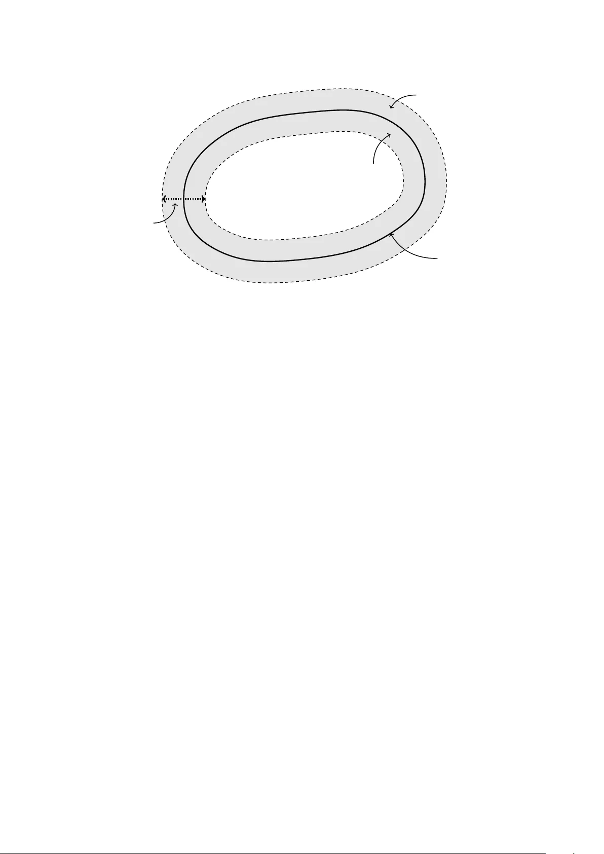
ON SOME MA THEMA TICAL PR OBLEMS F OR OPEN QUANTUM SYSTEMS WITH V AR YING P AR TICLE NUMBER BENEDIKT M. REIBLE AND LUIGI DELLE SITE Abstract. W e deriv e the effective Hamiltonian H − µN for open quantum systems with v arying particle n umber from first principles within the framework of non-relativistic quan tum statistical mec hanics. W e prov e that under ph ysically motiv ated assumptions regarding the size of the system and the range of the interaction, this form of the Hamiltonian is unique up to a constant. Our argumen t relies firstly on establishing a rigorous version of the surface-to-volume ratio approximation, which is routinely used in an empirical form in statistical mechanics, and secondly on showing that the Hilb ert space for systems with v arying particle num b er must b e isomorphic to F o ck space. T ogether, these findings provide a rigorous mathematical justification for the standard grand canonical formalism employ ed in statistical ph ysics. 1. Introduction 1.1. Prolegomenon. Realistic quan tum man y-b o dy systems are never truly isolated but rather exchange energy and p ossibly matter with their surroundings. Due to their practical relev ance, for example, in the developmen t of mo dern quantum technological devices, the theory of op en quan tum systems is a cornerstone of presen t-day theoretical and applied researc h [ 3 , 60 , 70 ]. While there are different elab orate mathematical frameworks in which to study these systems, e.g., the theory of op erator algebras [ 25 ] or Marko vian quantum master equations [ 45 ], numerous c hallenges regarding their theoretical description remain, esp ecially for systems with v arying particle num b er [ 18 ]. A deep er mathematical understanding of these systems is, how ever, not only desirable from a purely mathematical p oint of view, but it can also help, at first instance, to impro ve curren t state-of-the-art simulation techniques, whic h, in turn, can lead to new directions for the exp erimen tal realization of quantum systems for tec hnology [ 22 ]. F or an op en quan tum system with v arying particle n um b er, it is commonly accepted that the system’s Hilb ert space is given by F o ck space and that its Hamiltonian H should b e extended by the term − µN , with µ the chemical p oten tial and N the particle num b er op erator, resulting in the effe ctive Hamiltonian H − µN . (1) In the ph ysics literature, this op erator usually app ears implicitly in the deriv ation of the grand canonical density and, based on this, is defined to be the appropriate Hamiltonian for the op en system (see, e.g., Ref. [ 43 , p. 29]); the op erator ( 1 ) itself, how ev er, is not derived from first K ey wor ds and phr ases. Effective Hamiltonian, particle num ber op erator, chemical potential, F o ck space, surface-to-v olume ratio approximation. 1 2 B. M. REIBLE AND L. DELLE SITE principles. The use of an effectiv e Hamiltonian of the form ( 1 ) can be traced bac k at least to a conjecture by Bogoliub o v in the field of condensed matter physics [ 7 ], where it has b een used ev er since; see, for example, Ref. [ 73 , p. 314] and references therein. Also in mathematical ph ysics, it has b ecome common practice to analyze functional-an alytic properties of the op erator ( 1 ) and to build physical mo dels with its help; see, e.g., Ref. [ 8 , passim]. Recen tly , a semi-empirical deriv ation of Eq. ( 1 ) was prop osed, obtaining the effective Hamiltonian for an op en system b y tracing out the degrees of freedom of the reserv oir from the v on Neumann equation of the combined system [ 23 ]. While this study put forw ard imp ortan t ideas (on which we will actually build our analysis), the approac h also relied on some empirical assertions and formal manipulations. The goal of the present article is to provide a fully rigorous deriv ation of the effectiv e Hamiltonian ( 1 ) from first principles — starting from the total Hamiltonian of an op en system coupled to a reservoir, in tro ducing basic physical assumptions, and finally showing how the c hemical p oten tial µ emerges. In addition, w e will argue that the form of the effective Hamiltonian is unique up to additiv e constan ts. This will bridge the gap b etw een studies concerned with the mathematical foundations of quan tum mechanics, i.e., those dealing with general Hamiltonians and their prop erties, and studies fo cusing on sp ecific mathematical problems for grand canonical systems, where the Hamiltonian ( 1 ) is tak en for granted. 1.2. Main Results. T o deriv e an expression like ( 1 ) , we will hav e to analyze the general mathematical structure of an op en quan tum system with v arying particle num b er in a broader con text and establish some preparatory prop ositions. Our first result (Prop osition 3.4 ) provides a mathematically rigorous foundation for the so-called surface-to-volume ratio approximation. The latter is commonly used in statistical mec hanics when deriving the canonical or grand canonical density op erator; it consists of neglecting the interaction term H int in the total Hamiltonian H S ⊗ Id R + Id S ⊗ H R + H int for a system–reservoir comp osite. Deferring the details to Section 3 , we will show that: (I) Under some physic al ly justifie d assumptions on the system–r eservoir inter action and the r elative size of the op en system c omp ar e d to the r eservoir, it holds that E ρ [ H S ⊗ Id R + Id S ⊗ H R + H int ] ≈ E ρ [ H S ⊗ Id R + Id S ⊗ H R ] , up to higher-or der terms in the effe ctive inter action distanc e. The pro of of this assertion is geometric in nature, relying on certain results from con v ex geometry , and it highlights that a negligible surface-to-volume ratio is indeed required for the v alidity of the appro ximation. A v arying particle num b er will b ecome relev ant for our second result (Prop osition 4.2 ), which is indep endent of (I) . It pro vides a ph ysically motiv ated and mathematically rigorous argumen t for the necessity of F o ck space when describing quantum systems with the aforementioned c haracteristic: (I I) If ther e exists a total p article numb er op er ator with physic al ly r e asonable pr op erties (pur e p oint sp e ctrum and n -p article eigensp ac es), then the kinematic al structur e of the system is given in terms of F o ck sp ac e. OPEN QUANTUM SYSTEMS WITH V AR YING P AR TICLE NUMBER 3 Our pro of of this statemen t in Section 4 relies on standard metho ds from sp ectral theory as w ell as a recent, v ery general result on direct sums in W ∗ -categories. As discussed in detail in Remark 4.3 (1) , assertion (I I) should be seen as complemen ting similar results in the literature on the F o ck represen tation. Based on the previous t wo results (I) and (I I) , we will b e able to prov e our main result (Theorem 5.1 ) regarding the effectiv e Hamiltonian in Section 5 and show that the form ( 1 ) of this op erator, in the sp ecific physical setting considered, is unique up to a constant: (I II) If the surfac e-to-volume r atio appr oximation c an b e applie d and the p article numb er is varying, then H S ⊗ Id R + Id S ⊗ H R ≈ ( H S − µN ) ⊗ Id R , up to higher-or der terms in the p article numb er of the op en system. 1.3. Outline of the pap er. After in tro ducing the general mathematical setup and the basic ph ysical assumptions in Section 2 , we first discuss some preliminary observ ations on computing exp ectation v alues of unbounded op erators with resp ect to mixed quantum states (densit y op erators). In Section 3 , w e introduce sp ecific assumptions on the system–reserv oir in teraction, establish an auxiliary geometric result concerning quantitativ e b ounds for the interaction v olume, and then pro v e the v alidity of the surface-to-v olume ratio appro ximation. Next, Section 4 introduces the assumption of a v arying particle n umber in terms of the existence of a particle num ber op erator, and w e sho w that this necessarily leads to F o ck space. Finally , in Section 5 we syn thesize these results in order to deriv e the effectiv e Hamiltonian ( 1 ) . As a corollary , w e show that from this Hamiltonian one obtains an equiv alent of the hierarch y of v on Neumann equations derived in Ref. [ 23 ]. 1.4. Notation. T o conclude the introduction, let us fix some notation, frequen tly employ ed throughout the text, which is not used uniformly in the literature. F or d ∈ N and a Borel subset X ⊆ R d , we will denote its d -dimensional Leb esgue measure b y v ol ( X ) or λ d ( X ) , and its ( d − 1) -dimensional Hausdorff measure b y area ( X ) . F urthermore, B d = { x ∈ R d : | x | < 1 } and S d − 1 = { x ∈ R d : | x | = 1 } will denote the Euclidean unit ball and unit sphere, resp ectively , B d ( a, r ) = { x ∈ R d : | x − a | < r } denotes the ball of radius r > 0 around a ∈ R d , and ω d : = v ol( B d ) is the volume of the unit ball. General Hilb ert spaces will b e denoted by v arian ts of the symbol H , and inner pro ducts are written as ⟨· , ·⟩ ; the latter are taken to b e linear in the second and semi-linear in the first argumen t. The symbol L ( H ) denotes the set of all linear op erators T : H ⊇ dom ( T ) → H (generally unbounded) defined on a subspace dom ( T ) of H , B ( H ) ⊆ L ( H ) will b e the space of all everywhere-defined b ounded linear op erators on H , and finally B 1 ( H ) ⊆ B ( H ) denotes the space of all trace-class op erators on H . 2. Basic physical assumptions and ma thema tical setup T o set the stage, we introduce tw o basic h yp otheses, Assumptions A1 and A2 , whic h c haracterize the physical systems under in vestigation and provide the basis for the underlying mathematical mo del; we also use the opp ortunity to fix notation. In Section 2.3 , we establish a partial trace formula for un b ounded operators, which is central for deriving our main results. 4 B. M. REIBLE AND L. DELLE SITE 2.1. Op en quantum systems. Consider a large, isotropic quantum system, referred to as the total system T , consisting of N ∈ N particles 1 confined to a region Ω ⊆ R d , d ∈ N , of v olume V : = v ol ( Ω ) > 0 . Let H T b e the Hilb ert space and H T ∈ L ( H T ) b e the self-adjoint Hamiltonian describing the physics of T . The foundation for all the subsequen t inv estigations is the following basic mo deling assumption, which is the usual starting p oin t in the theory of op en quantum systems (see, for example, Refs. [ 9 , 17 , 70 ]): Assumption A1 (Division of the total system) . The total system T is divided into tw o in teracting subsystems: (1) the op en system S , which con tains N S ∈ N particles of interest and is confined to a b ounded and conv ex subregion Ω S ⊆ Ω of v olume V S : = v ol( Ω S ) < + ∞ ; (2) the r eservoir R , which is the remainder of T without S , thus it contains N R : = N − N S particles confined to the region Ω R : = Ω \ Ω S of volume V R : = v ol( Ω R ) > 0 . Regarding the physical scale of these tw o systems, we will assume that the op en system is macroscopic, yet significan tly smaller than the reservoir (and hence the total system), which is typical in statistical mec hanics [ 38 , p. 149]: A1.1. 1 ≪ N S ≪ N R and 1 ≪ V S ≪ V R . Finally , we will only b e concerned with equilibrium (or near-equilibrium) situations and hence also p ose the following assumption: A1.2. The systems S and R ha ve reac hed thermo dynamic equilibrium. Remarks 2.1. (1) Starting with the total system T and then dividing it in to the subsystems S and R , whic h hav e to b e chosen according to certain ph ysical requirements (like Assumption A1.1 and others following b elo w), facilitates a first-principle approach b ecause no sp ecific reservoir mo del is assumed. The opp osite pro cedure, i.e., taking the op en system and reservoir as giv en and then defining the total system, would lead to the same physics for the system S , presupp osing, how ever, information ab out the reserv oir and hence rendering the following in v estigations partially empirical. (2) Assuming that the op en system is confined to a b ounded region is necessary in order to ensure that it is thermo dynamically stable at p ositiv e temp erature [ 37 , Rem. 3]; see also Refs. [ 42 , p. 252] and [ 51 , Thm. XI I I.76]. Moreov er, since S is assumed to b e macroscopic and the total system is isotropic, the condition that Ω S should b e conv ex, while restricting mathematical generality , is nev ertheless rather natural from a ph ysical p oint of view. Corresp onding to the division of the total system T , w e will assume, in accordance with the usual axioms of quan tum mechanics [ 47 , Axiom A7, p. 844], that H T factorizes tensorially 1 With the term “particles”, we do not only mean elementary particles, but also larger comp osites that b ehav e quan tum-mechanically , e.g., molecules. OPEN QUANTUM SYSTEMS WITH V AR YING P AR TICLE NUMBER 5 in to a Hilb ert space H S of the op en system and a Hilb ert space H R of the reserv oir: H T = H S ⊗ H R . (2) Let H S ∈ L ( H S ) and H R ∈ L ( H R ) denote the self-adjoin t Hamiltonians for the degrees of freedom of the op en system and the reservoir, resp ectiv ely . Building on Eq. ( 2 ), the total Hamiltonian H T can b e written formally as [ 17 , p. 149] H T = H S ⊗ Id R + Id S ⊗ H R + H int , (3) where the op erator H int ∈ L ( H S ⊗ H R ) mediates the interaction b etw een S and R . Since H 0 : = H S ⊗ Id R + Id S ⊗ H R is essentially self-adjoint [ 52 , Thm. VI I I.33], [ 62 , Thm. 7.23], the op erator H int m ust b e chosen such that H T is essen tially self-adjoint as well, e.g., as an appropriate p erturbation of H 0 (see also Example 2.3 b elow). The mathematical setup discussed so far is illustrated in Fig. 1 . Lo oking no w at the in ternal structure of the op en system only , if H i denotes the Hilb ert space of the i -th particle in S , i ∈ { 1 , . . . , N S } , then similarly to Eq. ( 2 ) we ha v e H S = N S O i =1 H i . (4) Let us write h i ∈ L ( H i ) for the non-interacting self-adjoint Hamiltonian of the i -th particle in S suc h that H S tak es the form H S = N S X i =1 h i + H S , int , (5) where H S , int ∈ L ( H S ) contains the in teractions b etw een particles in S , and P N S i =1 h i is an abbreviation for the more precise (but cumbersome) expression N S X i =1  Id H 1 ⊗ · · · ⊗ Id H i − 1 ⊗ h i ⊗ Id H i +1 ⊗ · · · ⊗ Id H N S  . T o ensure stability of matter, we will assume, without loss of generalit y , that h i is a p ositiv e op erator for all i ∈ { 1 , . . . , N S } ; in this case, H S , 0 : = P N S i =1 h i is self-adjoin t and p ositive as w ell [ 2 , Thm. 3.8 (iv)], [ 62 , Thm. 7.23]. Remark 2.2. One should k eep in mind that for indistinguishable particles, the tensor pro duct in Eq. ( 4 ) has to be replaced b y the symmetric or anti-symmetric tensor pro duct of the Hilb ert spaces H i . Moreo ver, instead of simply assuming that there are N S particles in S , one has to consider all p ossible wa ys of taking N S particles from the total system consisting of N particles, whic h results in an additional combinatorial prefactor  N N S  to quan tities like the densit y op erator of the system [ 23 ]. In the follo wing, w e will not deal explicitly with these consequences of indistinguishabilit y but leav e the matter at this remark. 6 B. M. REIBLE AND L. DELLE SITE T otal System T ( H T , H T ) Ω Ω = Ω S ∪ Ω R , N = N S + N R Op en System S ( N S , H S , H S ) Ω S Reserv oir R ( N R , H R , H R ) Ω R = Ω \ Ω S H int Figure 1. Division of the total system according to Assumption A1 . 2.2. In teractions. Coming to the in teraction op erators H int and H S , int , w e will mak e the follo wing simplifying assumption throughout the pap er, whic h is t ypically sufficient for the needs of mathematical quantum mec hanics [ 42 , p. 44]. Assumption A2 (T w o-b o dy interactions) . The in teraction b etw een particles within the op en system as well as b etw een particles from the op en system and the reserv oir is of tw o-b ody t ype, meaning that for all pairs ( i, j ) and ( i, k ) of particle indices i, k ∈ { 1 , . . . , N S } , j ∈ { 1 , . . . , N R } , i  = k , there exist op erators V ij acting in H S ⊗ H R and W ik acting in H S suc h that H int = N S X i =1 N R X j =1 V ij and H S , int = N S X i =1 N S X k>i W ik . (6) Moreo v er, we will assume that these op erators can b e chosen so as to render the Hamiltonians H T = H 0 + H int and H S = H S , 0 + H S , int (essen tially) self-adjoint. Example 2.3. In the standard mathematical mo del of non-relativistic quan tum mechanics [ 47 , Axiom A5, p. 624], the Hilb ert space of a single particle from the op en system is given b y L 2 ( Ω S , λ d ) , hence [ 47 , Prop. 10.28] H S = O N S L 2 ( Ω S , λ d ) ∼ = L 2  Ω N S S , λ dN S  . The op erators h i are formally given by h i = − ℏ 2 2 m ∆ i + φ ( x i ) , where ∆ i is the Laplacian of the i - th particle’s co ordinates (with suitable b oundary conditions) and φ ( x i ) is an external p otential. If U : R d × R d → R , ( x, y ) 7→ U ( | x − y | ) , denotes the interaction p oten tial, then one may first consider the multiplication op erator M U acting in L 2 ( Ω S × Ω S , λ 2 d ) = L 2 ( Ω S , λ d ) ⊗ L 2 ( Ω S , λ d ) , and then construct W ik ∈ L ( H S ) as follo ws: W ik : = Id H 1 ⊗ · · · ⊗ Id H i − 1 ⊗ M U ⊗ Id H i +1 ⊗ · · · ⊗ Id H k − 1 ⊗ Id H k +1 ⊗ · · · ⊗ Id H N . OPEN QUANTUM SYSTEMS WITH V AR YING P AR TICLE NUMBER 7 Note that since N N S i =1 H i ∼ = N N S i =1 H σ ( i ) for any p ermutation σ of the set { 1 , . . . , N } , W ik is w ell-defined. An analogous pro cedure leads to the op erator V ij app earing in H int . In order to satisfy in this L 2 -picture the requiremen t that H S (and H T ) are (essen tially) self-adjoin t op erators, one should choose the p otential U , for example, from an appropriate class of p erturbations, namely , the Kato-Rellich class or the Rollnik class, in order to apply the Kato-Rellich or KLMN theorem; see, e.g., Refs. [ 50 , Sects. X.2 and X.4] and [ 62 , Sects. 8.3 and 10.7] as well as Refs. [ 64 , 65 ]. 2.3. Densit y op erators. Let S ( H ) denote the set of all density op erators on some Hilb ert space H , that is, the set of all p ositive trace-class op erators ρ ∈ B 1 ( H ) satisfying tr H ( ρ ) = 1 . It is w ell-known (see, e.g., Ref. [ 6 , Thm. 26.9]) that ρ ∈ S ( H ) if and only if there exist (i) a sequence ( α n ) n ∈ N ⊆ [0 , 1] with P n ∈ N α n = 1 and (ii) an orthonormal basis ( e n ) n ∈ N ⊆ H (ONB for short) such that ρ = ∞ X n =1 α n P e n , where P e n : = | e n ⟩⟨ e n | denotes the pro jection onto the one-dimensional subspace spanned by the vector e n , that is, the op erator P e n ξ : = ⟨ e n , ξ ⟩ e n ( ξ ∈ H ). While for b ounded op erators A ∈ B ( H ) the expression tr ( Aρ ) is alw ays w ell-defined since B 1 ( H ) is a tw o-sided ideal in B ( H ) , this need not b e the case for unbounded T ∈ L ( H ) due to domain issues. In the literature, there are different necessary and sufficient conditions ensuring that T ρ ∈ B 1 ( H ) ; see, for example, Refs. [ 47 , Prop. 11.27] and [ 48 , Prop. 4.59]. In this pap er, we will use a more direct approach, inspired b y Ref. [ 42 , Eq. (3.1.26)], to make sense of expressions of the form tr( T ρ ) for un b ounded T . Definition 2.4 (Compatible densit y op erators) . Let T ∈ L ( H ) b e self-adjoint. Define S ( H , T ) : =      ρ ∈ S ( H ) : ∃ ( e n ) n ∈ N ⊆ dom ( T ) ∃ ( α n ) n ∈ N ⊆ [ 0 , 1] : (i) ( e n ) n ∈ N is an ONB for H and P n ∈ N α n = 1 ; (ii) ρ = P n ∈ N α n P e n ; (iii) P n ∈ N α n |⟨ e n , T e n ⟩| < + ∞      and call the elemen ts of this set T -c omp atible density op er ators . F urthermore, for any ρ ∈ S ( H , T ) define the quantit y tr( T ρ ) by tr( T ρ ) : = ∞ X n =1 α n ⟨ e n , T e n ⟩ . (7) Note that since the series on the right-hand side of ( 7 ) con v erges absolutely b y assumption, tr ( T ρ ) is a real num ber, interpreted as the exp ectation v alue of T in the mixed state ρ . W e will, therefore, also use the notation E ρ [ T ] : = tr( T ρ ) . In App endix A , we sho w that our definition of T -compatible density op erators is meaningful b y establishing that the v alue of tr ( T ρ ) do es not dep end on the representation of ρ ∈ S ( H , T ) , and that for suitable T there holds S ( H , T )  = ∅ . 8 B. M. REIBLE AND L. DELLE SITE Denote by tr R : B 1 ( H S ⊗ H R ) → B 1 ( H S ) the partial trace op eration on H T with resp ect to H R , that is, for every trace-class op erator ρ on H S ⊗ H R , tr R ( ρ ) is the unique trace-class op erator on H S whic h satisfies for all A ∈ B ( H S ) [ 5 ], [ 6 , Cor. 26.5]: tr H S ⊗H R  ( A ⊗ Id R ) ρ  = tr H S  A tr R ( ρ )  . Belo w, we will need this identit y also for unbounded op erators. With the help of Definition 2.4 , the following result, whose pro of we giv e in App endix A.2 , obtains. Lemma 2.5. L et T ∈ L ( H S ) b e self-adjoint and ρ ∈ S ( H S ⊗ H R , T ⊗ Id R ) b e a T ⊗ Id R - c omp atible density op er ator. Then tr R ( ρ ) ∈ S ( H S , T ) and tr H S ⊗H R  ( T ⊗ Id R ) ρ  = tr H S  T tr R ( ρ )  . (8) In Section 3 , w e will b e interested in density op erators ρ on H T for which the exp ected energies E ρ S [ H S ] of S and E ρ R [ H R ] of R as well as the exp ected in teraction energy E ρ [ H int ] are w ell-defined; therefore, we in tro duce the following set of admissible density op er ators : 2 S (1) adm ( H T ) : = S ( H T , H S ⊗ Id R ) ∩ S ( H T , Id S ⊗ H R ) ∩ S ( H T , H int ) . (9) As a sp ecial case of Lemma A.4 , we obtain the relation S (1) adm ( H T ) ⊆ S ( H T , H T ) . (10) 3. Surf ace-to-v olume ra tio appro xima tion When discussing the division of a large system in to t w o subsystems in statistical mec hanics, the interaction betw een these subsystems (that is, the op erator H int in our case) is usually neglected based on the reason that it represents surface effects, which are negligible compared to the bulk energies of the subsystems; see, for example, Ref. [ 38 , pp. 131, 149] as well as Ref. [ 63 , pp. 38, 50]. This is expressed mathematically as H T ≈ H S + H R , (11) with the commen t that the op erator H int , while necessary for the equilibration of the tw o subsystems S and R , is “negligibly small” compared to the op erators H S and H R [ 63 , p. 50]; Eq. ( 11 ) is known as the surfac e-to-volume r atio appr oximation [ 38 , p. 131]. Since the in volv ed op erators H S , H R , and H int are unbounded, in general, one cannot simply compare their norms to determine whether H int is small compared to H S and H R . Therefore, in the follo wing, we shall mak e the appro ximation ( 11 ) mathematically precise in a framew ork that can handle unbounded op erators, and we will see in what sp ecific sense H int can b e neglected compared to H S and H R . Our pro of will also show that a negligibly small surface-to-v olume ratio is indeed crucial for the v alidity of the appro ximation. 2 W e note that the superscript “(1)” is added b ecause in Section 5 , we will consider a second class S (2) adm ( H T ) of admissible densit y op erators. OPEN QUANTUM SYSTEMS WITH V AR YING P AR TICLE NUMBER 9 3.1. Short-range interactions. As a first step tow ards a rigorous version of ( 11 ) , we need to form ulate an additional physical assumption on the system–reserv oir in teraction Hamiltonian H int , which is one of t w o essen tial requirements for the v alidit y of the approximation; in less precise terms, this assumption is also presen t in physical discussions of the surface-to-volume ratio approximation [ 38 , p. 131]. Assumption A3 (Interaction cutoff ) . There exists a num b er δ > 0 , whic h represents the effe ctive inter action distanc e b etw een particles from S and R , such that the op erator H int is determined only by those particles from Ω S and Ω R whose distance to each other is smaller than δ . Remarks 3.1. (1) Assumption A3 is natural in that for systems whic h are dominated by long-range in teractions b etw een the tw o subsystems S and R , one cannot exp ect to neglect the op erator H int compared to the other terms of the total Hamiltonian ( 3 ) . In this regard, it is in teresting to observ e that the Coulomb in teraction, which is the most imp ortan t interaction for ordinary matter but also characterized b y a slow deca y at infinit y , can b e considered to hav e a small effectiv e in teraction distance due to electrostatic screening which is a consequence of Newton’s theorem [ 41 , 42 ] (see also Refs. [ 36 , 37 ]); this fact is indeed essential for the existence of the thermo dynamic limit of Coulomb systems. In applied physics, the effective in teraction distance of the Coulomb p oten tial can often b e characterized in terms of the Deby e length; see Ref. [ 10 ] and references therein for the range of v alidit y of different screening mo dels. (2) F or sp ecific applications of the surface-to-volume ratio approximation, one m ust chec k whether the mo del under inv estigation satisfies Assumption A3 b y determining the effective in teraction distance of the mo del. As w e will sho w below, the error terms due to the appro ximation depend on δ , and thus, once the latter is kno wn, one can estimate the correction terms and decide whether the approximation is feasible or not. Assumption A3 implies that for a particle at p osition x ∈ Ω S , only those particles con tained within the ball B ( x, δ ) of radius δ around x will interact with it. Regarding inter-domain in teractions b etw een Ω S and Ω R , this means that all the in volv ed particles necessarily must b e lo cated in the tubular δ -neigh b orho od ( ∂ Ω S ) δ (cf. Definition B.1 in App endix B ) of the b oundary ∂ Ω S of the region Ω S : ( ∂ Ω S ) δ = [ z ∈ ∂ Ω S B ( z , δ ) =  y ∈ Ω : dist( y , ∂ Ω S ) < δ  . Note that since Ω = Ω S ∪ Ω R b y construction (Assumption A1 ), we ma y split ( ∂ Ω S ) δ in to an “outer” tubular neighborho o d ( ∂ Ω S ) + δ extending into Ω R , and an “inner” tubular neighborho o d ( ∂ Ω S ) − δ extending into Ω S , which are given b y ( ∂ Ω S ) + δ : =  y ∈ Ω R : dist( y , ∂ Ω S ) < δ  , ( ∂ Ω S ) − δ : =  x ∈ Ω S : dist( x, ∂ Ω S ) < δ  . 10 B. M. REIBLE AND L. DELLE SITE Ω R Ω S ∂ Ω S ( ∂ Ω S ) − δ ( ∂ Ω S ) + δ 2 δ Figure 2. Illustration of the set Ω S , circumscrib ed b y the solid line, and the interaction corridor ( ∂ Ω S ) + δ ∪ ( ∂ Ω S ) − δ of width 2 δ around its b oundary , highligh ted as the gray region delimited by the dashed lines. It clearly holds that ( ∂ Ω S ) δ = ( ∂ Ω S ) + δ ∪ ( ∂ Ω S ) − δ ; see also Fig. 2 for an illustration of the differen t inv olv ed sets. T o emphasize that this tubular neighborho o d has total width 2 δ , we shall denote it by the symbol Γ 2 δ ( Ω S ) : = ( ∂ Ω S ) + δ ∪ ( ∂ Ω S ) − δ = ( ∂ Ω S ) δ . In this terminology , Assumption A3 entails that all the particles from Ω S and Ω R captured b y H int lie inside the inter action c orridor Γ 2 δ ( Ω S ) . Let N int ≡ N int ( δ ) ∈ N b e the num b er of these particles. Then we may rewrite the interaction Hamiltonian from Eq. ( 6 ) as H int = N int X i =1 N int X j >i V ij . (12) 3.2. V olume of the interaction corridor. The main technical ingredien t for the surface- to-v olume ratio approximation is the following lemma, which provides an estimate for the v olume of the in teraction corridor Γ 2 δ ( Ω S ) in terms of the surface area of the b oundary ∂ Ω S and the interaction distance δ ; its pro of relies on established results in con v ex geometry that are summarized in App endix B . Lemma 3.2. A ssume that K ⊆ R d is a b ounde d c onvex domain. Then the volume of the c orridor Γ 2 δ ( K ) is b ounde d ab ove and b elow by δ · area( ∂ K ) + O ( δ 2 ) ≤ vol  Γ 2 δ ( K )  ≤ 2 δ · area( ∂ K ) + O ( δ 2 ) for δ → 0 . (13) Pr o of. First, note that using Definition B.1 of the tubular δ -neigh b orho od K δ of the set K , w e may express ( ∂ K ) + δ equiv alently as ( ∂ K ) + δ = K δ \ K . Since the outer and inner tubular neigh b orho ods of K are disjoin t, it follows from additivity of the Leb esgue measure that OPEN QUANTUM SYSTEMS WITH V AR YING P AR TICLE NUMBER 11 v ol  Γ 2 δ ( K )  = v ol  ( ∂ K ) + δ ∪ ( ∂ K ) − δ  = v ol  K δ \ K  + v ol  ( ∂ K ) − δ  . (14) W e shall consider b oth of the terms separately . F or the first one, observe that since K ⊆ K δ and v ol ( K ) < + ∞ , we hav e v ol ( K δ \ K ) = v ol ( K δ ) − vol ( K ) . Th us, w e can apply the Mink o wski-Steiner form ula (Theorem B.3 in App endix B ) to obtain v ol  K δ \ K  = area( ∂ K ) δ + O ( δ 2 ) for δ → 0 . (15) F or the second term, note that by definition, one has ( ∂ K ) − δ ⊆ { x ∈ K : dist( x, ∂ K ) ≤ δ } . Therefore, monotonicity of the Leb esgue measure and Lemma B.6 imply v ol  ( ∂ K ) − δ  ≤ vol  { x ∈ K : dist( x, ∂ K ) ≤ δ }  ≤ area ( ∂ K ) δ . Com bining the last three equations prov es the upp er b ound. F or the low er b ound, it suffices to note that v ol ( Γ 2 δ ( K )) ≥ vol ( K δ \ K ) b y Eq. ( 14 ), hence the estimate follows from ( 15 ) . ■ Remark 3.3. Let K ⊆ R d satisfy the assumptions of Lemma 3.2 and s uppose, in addition, that B d ⊆ K . Then the quermassintegrals W j ( K ) , j ∈ { 2 , . . . , d − 1 } , from Eq. ( 33 ) entering the Minko wski-Steiner formula can b e estimated using the fact that the mixed volume is non-decreasing in each argumen t (cf. Remark B.4 in App endix B and Ref. [ 33 , Thm. 6.9]): for all j ∈ { 2 , . . . , d − 1 } w e hav e the upp er b ound W j ( K ) = V  K, . . . , K | {z } d − j , B d , . . . , B d | {z } j  ≤ V  K, . . . , K | {z } d − 1 , B d  = W 1 ( K ) as well as the lo wer bound ω d = V  B d , . . . , B d  ≤ V  K, . . . , K | {z } d − j , B d , . . . , B d | {z } j  = W j ( K ) . Since W 1 ( K ) = 1 d area ( ∂ K ) , it follows that instead of usin g Eq. ( 15 ) in the ab o ve proof, we can apply the previous t wo estimates for W j ( K ) in the Mink owski-Steiner form ula ( 32 ) to obtain the upp er b ound v ol  K δ \ K  ≤ area ( ∂ K ) δ + d X j =2 1 d d j ! area( ∂ K ) δ j = area( ∂ K ) δ + O  area( ∂ K ) δ 2  for δ → 0 , where we used ω d ≤ W 1 ( K ) for the last term, and, similarly , the low er b ound v ol  K δ \ K  ≥ area ( ∂ K ) δ + O  ω d δ 2  for δ → 0 . These t w o estimates for v ol  K δ \ K  translate directly in to a corresp ondingly mo dified v ersion of the t wo-sided inequalit y ( 13 ): for δ → 0 we ha v e δ · area( ∂ K ) + O  ω d δ 2  ≤ vol  Γ 2 δ ( K )  ≤ 2 δ · area( ∂ K ) + O  area( ∂ K ) δ 2  . (16) 12 B. M. REIBLE AND L. DELLE SITE 3.3. F orm ulation of the approximation. W e can now formulate and pro v e the main result of this section; as the name suggests, the surface-to-volume ratio κ : = area( ∂ Ω S ) V S will play an imp ortan t role. In addition to Assumption A3 , the following prop osition also relies on another physical h yp othesis on κ as well as on a technical mathematical condition. Prop osition 3.4 (Surface-to-v olume ratio appro ximation) . Supp ose that A ssumption A3 holds true and that the effe ctive inter action distanc e δ > 0 sp e cifie d ther ein is r e asonably smal l. F urthermor e, supp ose that the r e gion Ω S is b ounde d, c onvex and lar ge enough such that A4. 2 δ · κ ≪ 1 and B d ⊆ Ω S . L et ρ ∈ S (1) adm ( H T ) b e an admissible density op er ator of the total system [ cf. Eq. ( 9 )] and assume, in addition, that A5. ρ ∈ \ 1 ≤ ii W ij # ρ S ! = N S X i =1 N S X j >i tr H S ( W ij ρ S ) ≥ N S X i =1 N S X j >i  min 1 ≤ k<ℓ ≤ N S tr H S ( W kℓ ρ S )  | {z } = : E < S , int = N S ( N S − 1) E < S , int ≈ N 2 S E < S , int , where the last approximation is v alid b ecause of N S ≫ 1 by Assumption A1.1 . In an analogous w a y , we can estimate E ρ S [ H S , int ] from ab o v e: E ρ S [ H S , int ] ≤ N S X i =1 N S X j >i  max 1 ≤ k<ℓ ≤ N S tr H S ( W kℓ ρ S )  | {z } = : E > S , int = N S ( N S − 1) E > S , int ≈ N 2 S E > S , int . Similarly , we can estimate E ρ [ H int ] from ab ov e and b elo w: using Eq. ( 12 ), Assumption A5 , and Lemma A.4 , it follows that E ρ [ H int ] = tr H T " N int X i =1 N int X j >i V ij # ρ ! = N int X i =1 N int X j >i tr H T ( V ij ρ ) ≤ N int X i =1 N int X j >i  max 1 ≤ k<ℓ ≤ N int tr H T ( V kℓ ρ )  | {z } = : E > int = N int ( N int − 1) E > int ≈ N 2 int E > int as well as E ρ [ H int ] ≥ N int X i =1 N int X j >i  min 1 ≤ k<ℓ ≤ N int tr H T ( V kℓ ρ )  | {z } = : E < int = N int ( N int − 1) E < int ≈ N 2 int E < int . Observ e that b y Assumption A5 , the quan tities E < S , int , E > S , int , E < int , E > int are all w ell-defined and finite. Using the previous four bounds (as w ell as our assumption b elow Eq. ( 19 ) whic h en tails E ρ [ H S ⊗ Id R ] = E ρ S [ H S , int ] ), we arriv e at the tw o-sided inequality N 2 int N 2 S E < int E > S , int ≤ E ρ [ H int ] E ρ [ H S ⊗ Id R ] ≤ N 2 int N 2 S E > int E < S , int . F or small enough δ , we can assume that the particle n umber densit y n int inside the in teraction corridor Γ 2 δ ( Ω S ) is constant, i.e., n int = N int / v ol  Γ 2 δ ( Ω S )  . This assumption is meaningful b ecause S and R are in thermo dynamic equilibrium (cf. Assumption A1.2 ), implying that the tw o parts ( ∂ Ω S ) − δ ⊆ Ω S and ( ∂ Ω S ) + δ ⊆ Ω R of the interaction corridor must ha v e the same particle num ber density . Therefore, w e can recast the previous b ound as n 2 int n 2 S E < int E > S , int | {z } = : C 1 v ol  Γ 2 δ ( Ω S )  V S ! 2 ≤ E ρ [ H int ] E ρ [ H S ⊗ Id R ] ≤ v ol  Γ 2 δ ( Ω S )  V S ! 2 n 2 int n 2 S E > int E < S , int | {z } = : C 2 , 14 B. M. REIBLE AND L. DELLE SITE where n S = N S /V S is the uniform particle n um b er densit y of the op en system S ; the constan ts C 1 , C 2 ∈ R dep end on the ph ysics of the op en system S and the interaction b et w een S and the reservoir R . F rom the refined volume estimate ( 16 ) of Remark 3.3 , which is applicable since B d ⊆ Ω S b y Assumption A4 , we obtain the following b ounds for δ → 0 : C 1  δ · κ + O  ω d V S · δ 2  2 ≤ E ρ [ H int ] E ρ [ H S ⊗ Id R ] ≤ C 2 h 2 δ · κ + O  κ · δ 2  i 2 . (20) A ccording to A4 , w e hav e assumed that the first terms in the tw o brack ets are v ery small and can hence b e neglected. Therefore, O  ω 2 d V 2 S · δ 4  ≤ E ρ [ H int ] E ρ [ H S ⊗ Id R ] ≤ O  κ 2 · δ 4  for δ → 0 . Since the constants ω 2 d /V 2 S and κ 2 are b oth very small, we can conclude that for δ → 0 , the energy ratio is of order O ( δ 4 ) . Returning now to the formula ( 18 ) for the exp ected energy of the total system, it follows that for δ → 0 : E ρ [ H T ] = E ρ [ H S ⊗ Id R ] 1 + E ρ [ H int ] E ρ [ H S ⊗ Id R ] ! + E ρ [Id S ⊗ H R ] = E ρ [ H S ⊗ Id R ]  1 + O  δ 4   + E ρ [Id S ⊗ H R ] = E ρ [ H S ⊗ Id R + Id S ⊗ H R ] + O  δ 4  . ■ Remarks 3.5. (1) The first expression in Assumption A4 is precisely the surface-to-volume ratio for the op en system’s region Ω S , m ultiplied b y the total width of the interaction corridor. Thus, this quantit y b eing small captures the intuitiv e idea that the interaction represents negligible surface effects. The second demand B d ⊆ Ω S is connected to the assumption that Ω S should b e large enough; in principle, this requiremen t is not strictly necessary for the pro of, but it allo ws us to apply the more controlled estimate ( 16 ) of Remark 3.3 . Observe that using the estimate ( 13 ) from Lemma 3.2 directly , one would also obtain the error b ound O ( δ 4 ) . (2) Assumption A5 is a technical necessit y to ensure that the computations in the pro of, namely the estimates for E ρ S [ H S , int ] and E ρ [ H int ] , are fully justified. Physically , this assumption en tails that the state ρ of the total system should b e chosen such that there is a well-defined exp ected in teraction energy b et ween all the inv olv ed particles, and similarly that in the reduced state ρ S the exp ected interactions are well-defined, to o. (3) The conclusion ( 17 ) of Prop osition 3.4 shows in what sense H int can b e neglected compared to the other comp onen ts of H T : for the total exp ected energy of T , H int only plays a negligible role. Since in statistical mechanics, the surface-to-volume ratio approximation is applied precisely when the energy of T is compared with the energies of S and R (see, e.g., Ref. [ 63 , pp. 50 f.]), Eq. ( 17 ) can indeed b e considered a useful formalization of the heuristic expression ( 11 ). OPEN QUANTUM SYSTEMS WITH V AR YING P AR TICLE NUMBER 15 (4) Finally , it should b e men tioned that in the past we hav e already linked the surface- to-v olume ratio approximation empirically to the so-called tw o-sided Bogoliub o v inequality , whic h provides upp er and lo wer bounds for the free energy cost of separating a large system in to indep endent subsystems [ 55 , 56 , 57 ]. Example 3.6. W e shall consider tw o sp ecial situations in whic h the error estimate O ( δ 4 ) of Prop osition 3.4 can b e strengthened. (1) Supp ose that d = 3 . In this case, the Mink owski-Steiner form ula ( 32 ) for the volume of ( ∂ Ω S ) + δ = ( Ω S ) δ \ Ω S has only three terms: v ol  ( ∂ Ω S ) + δ  = area( ∂ Ω S ) δ + 3 W 2 ( Ω S ) δ 2 + ω 3 δ 3 . As shown in Example B.5 , we ha v e W 2 ( Ω S ) ≤ ω 3 diam ( Ω S ) b ecause 0 ∈ Ω S b y the assumption B d ⊆ Ω S . Since also ω 3 ≤ W 2 ( Ω S ) (cf. Remark 3.3 ), it follows that in case d = 3 the tw o estimates for Γ 2 δ ( Ω S ) b ecome δ · area( ∂ Ω S ) + 3 ω 3 δ 2 + ω 3 δ 3 ≤ vol  Γ 2 δ ( Ω S )  ≤ 2 δ · area( ∂ Ω S ) + 3 ω 3 diam( Ω S ) δ 2 + ω 3 δ 3 . Using this inequality instead of Eq. ( 16 ) in the pro of of Prop osition 3.4 , the upp er b ound on the ratio of energies in Eq. ( 20 ) turns into E ρ [ H int ] E ρ [ H S ⊗ Id R ] ≤ C 2 " 2 δ · κ + 3 ω 3 diam( Ω S ) δ 2 V S + ω 3 δ 3 V S # 2 . (The lo wer b ound remains structurally the same.) The first and the last expression in the square brack ets are negligible. It therefore follows that the ratio is con trolled b y the term 3 ω 3 diam( Ω S ) δ 2 v ol( Ω S ) . A sufficien t condition to ensure that this is negligible as well is to assume that the set Ω S is large enough as to contain a ball of radius 1 p diam ( Ω S ) ≫ 1 , p ∈ N . In this case, v ol( Ω S ) ≥ ω 3 diam( Ω S ) 3 /p 3 and hence it follows that 3 ω 3 diam( Ω S ) δ 2 v ol( Ω S ) ≤ 3 p 3  δ diam( Ω S )  2 ≪ 1 . (2) Consider again an arbitrary d ∈ N but supp ose that Ω S = B d (0 , R ) is the ball of radius R ≫ 1 . It holds that ∂ Ω S = S d − 1 (0 , R ) is the sphere of radius R , and hence the interaction corridor is giv en by (see also Ref. [ 49 , p. 1189]) Γ 2 δ ( Ω S ) = ( ∂ Ω S ) δ = B d (0 , R + δ ) \ B d (0 , R − δ ) . Its volume can b e computed explicitly: v ol  Γ 2 δ ( Ω S )  = ω d h ( R + δ ) d − ( R − δ ) d i = 2 ω d X 1 ≤ k ≤ d k o dd d k ! R d − k δ k , 16 B. M. REIBLE AND L. DELLE SITE where the binomial theorem w as used. Since vol( Ω S ) = ω d R d , it follo ws that v ol  Γ 2 δ ( Ω S )  v ol( Ω S ) = 2 X 1 ≤ k ≤ d k o dd d k ! R − k δ k . (21) The crucial ph ysical criterion guaranteeing a negligible su rface-to-v olume ratio is δ R ≪ 1 b ecause in this case, the estimate ( 20 ) of the pro of of Prop osition 3.4 b ecomes C 1 " 4 d 2  δ R  2 + O  δ R  4 # ≤ E ρ [ H int ] E ρ [ H S ⊗ Id R ] ≤ C 2 " 4 d 2  δ R  2 + O  δ R  4 # . Supp ose now that d = 3 . In this case, there are only tw o terms in the surface-to-volume ratio ( 21 ) ; hence, we can write do wn the summands in the square brack ets app earing in the upp er and low er b ound, obtained b y squaring Eq. ( 21 ), explicitly: 36  δ R  2 + 24  δ R  4 + 4  δ R  6 . 4. V ar ying p ar ticle number and F ock sp ace In the next step, w e wan t to analyze some immediate consequences of the additional ph ysical feature that the total particle num ber in the op en system S is v arying. Throughout the literature, it is usually taken for granted that in this case the Hilb ert space H S is equal to F o c k space [ 28 , 15 ]; see, for example, the textb o oks [ 35 , 61 ] which are among the most rigorous in their field. In the following, w e will provide a conceptually simple pro of, relying on a technically inv olved result, of the fact that under physically well-motiv ated assumptions, the Hilb ert space H S m ust indeed b e isomorphic to F o ck space, i.e., the kinematical structure of S is necessarily give n in terms of F o c k space. 4.1. P article num b er op erator. T o start, w e will p ose another key physical assumption, whic h implements the feature of a v arying particle n umber in terms of a num ber op erator with sp ecific prop erties. Assumption A6 (V arying particle num ber) . Supp ose that the op en system S consists of iden tical particles, let H denote the one-particle Hilb ert space of this species, and assume that the total particle num ber N S ∈ N of S is v arying. Then we p ose that A6.1. H ⊗ n ⊆ H S for all n ∈ N 0 with isometric em b edding. (W e set H ⊗ 0 : = C .) A ccording to the standard description of quan tum mechanics, the Hilb ert space H ⊗ n : = N n H is the state space for an n -particle system (recall Remark 2.2 in this context), hence the space H S m ust contain all these to correctly describ e all p ossible states with different particle n um b ers. The embedding should b e isometric in order to guarantee that a pure state (that is, a normalized v ector) in H ⊗ n is also a pure state in H S . Second, we pose: OPEN QUANTUM SYSTEMS WITH V AR YING P AR TICLE NUMBER 17 A6.2. There exists a self-adjoint op erator N ∈ L ( H S ) such that (i) σ ( N ) = σ p ( N ) = N 0 and (ii) Eig( N , n ) = H ⊗ n for all n ∈ N 0 . Since the particle num b er is not merely a parameter an ymore but a ph ysical observ able, there should b e a self-adjoint op erator representing this observ able whose sp ectral v alues are precisely the different possible particle num bers and which yields the n umber n on the n -particle subspace H ⊗ n . Remark 4.1. In ordinary , non-relativistic quantum matter, the particle num ber op erator is t ypically defined in terms of creation and annihilation op erators, and the latter are used to generate and remo ve excitations of physical particles whose num ber within the op en system is fixed, but not to exc hange the particles themselv es with the reservoir. A truly v arying particle num b er usually app ears in quantum field theory , where the creation and annihilation of elemen tary particles due to v acuum fluctuations is describ ed. In light of these tw o situations mostly treated in the literature, it must b e emphasized that w e treat existing physical particles, whic h constitute actual matter and not merely excitations, that can enter and exit the op en system, but are not created or destroy ed as in quantum field theory . F or a more detailed discussion of the difference b etw een the exchange of excitations and the exc hange of physical particles in the context of the Lindblad equation, we refer to Ref. [ 53 ]. Based on the physically motiv ated Assumption A6 , we obtain the following result; its pro of relies on a v ery general characterization of infinite direct sums of Hilb ert spaces in terms of a univ ersal prop erty [ 30 , Thm. 5.1], which is recalled in App endix C . Prop osition 4.2 (Necessit y of F o c k space) . A ssume that the Hilb ert sp ac e H S satisfies the assumptions A6.1 and A6.2 . Then it fol lows that H S = ∞ M n =0 H ⊗ n . (22) Pr o of. F or n ∈ N 0 , let i n : H ⊗ n  → H S , ξ 7→ i n ( ξ ) , denote the inclusion mapping, which is a well-defined isometry according to A6.1 , that is, ∥ i n ( ξ ) ∥ H S = ∥ ξ ∥ H ⊗ n . Using p olarization, one obtains ⟨ i n ( ξ ) , i n ( η ) ⟩ H S = ⟨ ξ , η ⟩ H ⊗ n for all ξ , η ∈ H ⊗ n , and this implies i ∗ n i n = Id H ⊗ n [ 14 , Prop. I I.2.17]. Moreov er, for n, m ∈ N with n  = m and ξ ∈ H ⊗ n , η ∈ H ⊗ m , we ha v e  ξ , i ∗ n i m ( η )  H ⊗ n =  i n ( ξ ) , i m ( η )  H S = 0 b ecause H ⊗ n = Eig ( N , n ) ⊥ Eig ( N , m ) = H ⊗ m b y A6.2 , since the eigenspaces of a self- adjoin t op erator are pairwise orthogonal [ 62 , Lem. 3.4]. This implies that i ∗ n i m = 0 for n  = m b ecause ξ , η were arbitrary; hence, in total, we ha v e for all n, m ∈ N 0 : i ∗ n i m = δ nm Id H ⊗ n . (23) Define the op erators P n : = i n i ∗ n ∈ B ( H S ) , n ∈ N 0 , and note that P ∗ n = P n and P 2 n = P n b y ( 23 ) , showing that the P n are orthogonal pro jections. Let ξ ∈ H ⊗ n b e arbitrary . It holds that P n i n ( ξ ) = i n i ∗ n i n ( ξ ) = i n ( ξ ) , so i n ( ξ ) ∈ ran ( P n ) which implies H ⊗ n ⊆ ran ( P n ) in H S . Next, 18 B. M. REIBLE AND L. DELLE SITE let Φ ∈ ( H ⊗ n ) ⊥ ⊆ H S , i.e., ⟨ Φ, i n ( ξ ) ⟩ H S = 0 for all ξ ∈ H ⊗ n . If Ψ ∈ H S , it follo ws that  Ψ , P n Φ  H S =  i n i ∗ n ( Ψ ) , Φ  H S = 0 , and thus, since Ψ w as arbitrary , Φ ∈ ker ( P n ) which implies ( H ⊗ n ) ⊥ ⊆ ker ( P n ) . As P n is an orthogonal pro jection, k er ( P n ) = ran ( P n ) ⊥ and hence ( H ⊗ n ) ⊥ ⊆ ran ( P n ) ⊥ . This implies that if Ψ ∈ ran ( P n ) , then Ψ ⊥ Φ for all Φ ∈ ( H ⊗ n ) ⊥ and so Ψ ∈ ( H ⊗ n ) ⊥⊥ = H ⊗ n = H ⊗ n since H ⊗ n is a closed subspace of H S (as this space is complete and i n is an isometry). W e conclude that ran ( P n ) ⊆ H ⊗ n ; hence, we hav e equality ran ( P n ) = H ⊗ n . Therefore, P n m ust b e the unique orthogonal pro jection onto the closed subspace H ⊗ n ⊆ H S . Let E N denote the sp ectral measure of the self-adjoint op erator N . It holds that E N ( { n } ) , n ∈ N 0 , is the orthogonal pro jection in H S on to the space Eig ( N , n ) = H ⊗ n [ 62 , Prop. 5.10], and thus the previous result implies that E N ( { n } ) = P n = i n i ∗ n . F rom countable additivit y of the sp ectral measure, w e can now deriv e the follo wing identit y: ∞ X n =0 i n i ∗ n = ∞ X n =0 E N  { n }  = E N  ∞ [ n =0 { n }  = E N  σ ( N )  = Id H S . (24) In light of Eqs. ( 23 ) and ( 24 ), we ma y inv ok e the univ ersal prop erty of the Hilb ert space direct sum, see Theorem C.1 in App endix C , to conclude that H S m ust b e the direct sum of the spaces H ⊗ n , which pro v es the claim. ■ Remarks 4.3. (1) Qualitativ ely , the assertion of Prop osition 4.2 ma y b e summarized as follows: if there exists a total particle num ber op erator on H S , then H S has to b e the F o ck space. In this con text, it m ust be noted that the connection b et ween the existence of a num b er op erator and F o ck space has b een studied intensiv ely in the literature on represen tations of the canonical (an ti-)comm utation relations [ 12 , 13 , 16 , 20 , 21 , 29 , 34 , 72 ] (references in alphab etical order); see, in particular, Ref. [ 12 , pp. 23–25] for a summary of the v arious results and also the textb ook accounts [ 8 , pp. 30 ff.] and [ 67 , pp. 21 f.]. In essence, these studies show ed that an op erator of the form N = P ∞ k =1 a ∗ k a k , where a ∗ k and a k are the creation and annihilation op erators, resp ectiv ely , exists only in a direct sum of F o c k representations of the canonical (an ti-)commutation relations. (Different mathematical inter pretations of the conv ergence of the series P ∞ k =1 a ∗ k a k of unbounded op erators as w ell as alternativ e definitions of a num ber op erator were in v estigated in Refs. [ 12 , 13 , 20 ].) The nov elt y of Proposition 4.2 compared to the list of references giv en ab o ve, aside from the one already discussed in Remark 4.1 , is that it did neither require the abstract mathematical framew ork of algebraic quantum field theory nor a mathematically in volv ed definition of the n um b er op erator in terms of creation and annihilation op erators; in fact, the c haracterization of a total particle num b er op erator as in A6.2 is mathematically simple but also physically v ery w ell motiv ated. Moreo ver, relying on a category-theoretic result for the characterization of the infinite direct sum of Hilbert spaces (cf. App endix C ) connects the physical assumptions A6.1 and A6.2 with the mathematically fundamental univ ersal prop erty of the direct sum. OPEN QUANTUM SYSTEMS WITH V AR YING P AR TICLE NUMBER 19 (2) In recent y ears, there has b een increased in terest in the physical feature of a v arying particle num ber in the framework of classical mechanics; see, for example, Refs. [ 18 , 19 , 24 , 40 ] and references therein. Hence, it is w orthwhile to discuss Prop osition 4.2 in this context. Since there is no canonical notion of a classical F o c k space, one has to model the configuration space of a classical system with v arying particle n umber in terms of a hierarch y of h yp erplanes of configuration spaces with fixed particle num ber. These hyperplanes are connected by dynamical transition probabilities (free energy), which are determined based on statistical mec hanics considerations. Th us, Proposition 4.2 shows that in quantum mechanics the mathematical framework for systems with v arying particle num b er is more compact, a fact that is also reflected by Corollary 5.3 b elow. Ho wev er, it must b e noted that Ref. [ 19 ] put forw ard the prop osal to use a F o ck space formalism in a classical framew ork, suitably adapted to the ph ysical situation, to mo del particle-based reaction–diffusion pro cesses. Corollary 4.4. If the total p article numb er N S of S is varying and b ounde d ab ove by M ∈ N , then the Hilb ert sp ac e of S is given by the finite dir e ct sum H S = M M n =0 H ⊗ n . Pr o of. Under the additional assumption on N S , it follows that A6.1 and A6.2 m ust b e mo dified b y replacing the set N 0 with { 0 , 1 , . . . , M } . The pro of then pro ceeds as ab ov e by in voking Theorem C.1 from App endix C with index set I = { 0 , 1 , . . . , M } . ■ 4.2. Direct sum op erators. Before moving on, we quic kly recall how the Hamiltonian of the op en system S c hanges due to the transition from the N S -fold tensor pro duct space ( 4 ) to the F o c k space ( 22 ), denoted in the following as F ( H ) : = ∞ M n =0 H ⊗ n . Recall the general definition of the Hilb ert space direct sum, provided in Eq. ( 34 ) in App endix C , and for ev ery n ∈ N 0 let H S ,n ∈ L ( H ⊗ n ) denote the Hamiltonian of an n - particle realization of the op en system S , that is, H S ,n is given b y Eqs. ( 5 ) and ( 6 ), with N S replaced by n . The appropriate Hamiltonian for S is the op erator H ∈ L  F ( H )  defined on the domain [ 2 , p. 195] dom( H ) : =     ψ ( n )  n ∈ N 0 ∈ F ( H ) : ψ ( n ) ∈ dom ( H S ,n ) and X n ∈ N 0   H S ,n ψ ( n )   2 H ⊗ n < + ∞    , and it acts on an elemen t Ψ = ( ψ ( n ) ) n ∈ N 0 ∈ dom ( H ) by H Ψ : = ( H S ,n ψ ( n ) ) n ∈ N 0 . Due to this definition, one denotes the op erator H also by H = ∞ M n =0 H S ,n . 20 B. M. REIBLE AND L. DELLE SITE One can sho w that if the op erators H S ,n are all self-adjoin t (which we assumed), then H is also self-adjoin t [ 2 , Thm. 4.2 (vi)]. Similarly to the definition of H , the num b er op erator N ∈ L ( H S ) introduced in Assumption A6.2 may b e written as (cf. Ref. [ 2 , p. 221]) N = ∞ M n =0  n Id H ⊗ n  . In addition to the change of the Hamiltonian of the system, also the set of admissible density op erators first introduced in Eq. ( 9 ) has to b e up dated: on the one hand, the op erator H int mediating the system–reserv oir interaction do es not pla y a role anymore due to Prop osition 3.4 , and on the other hand, the physically relev ant densit y op erators no w hav e to b e compatible with the op erator N as w ell due to Assumption A6 . Therefore, we define S (2) adm ( H T ) : = S ( H T , H ⊗ Id R ) ∩ S ( H T , N ⊗ Id R ) ∩ S ( H T , Id S ⊗ H R ) . 5. The effective Hamil tonian W e ha ve established a rigorous v ersion of the surface-to-volume ratio approximation (Prop osition 3.4 ) as well as the necessity of F o c k space for systems with v arying physical particle num b er (Prop osition 4.2 ). Based on these results, w e can no w derive the effective Hamiltonian for the op en system S and argue that, given the necessary assumptions and relev ant appro ximations, it is unique up to a constan t. 5.1. Main result. In the sequel, we will build on ideas put forward in Ref. [ 23 ], where the same effective Hamiltonian was deriv ed based on semi-empirical assertions, but w e will follow a different, more rigorous approach; see Remark 5.2 b elow for a detailed discussion of the differences of the tw o approaches. Theorem 5.1 (Effective Hamiltonian) . Supp ose that the surfac e-to-volume r atio appr oximation has b e en applie d to the total system T , and that the op en system S satisfies A ssumption A6 . Set ε : = N S / N . Then ther e exists a c onstant µ ∈ R such that H T = ( H − µ N ) ⊗ Id R + O ( ε 2 ) . (25) The op er ator H eff : = H − µ N ∈ L ( H S ) is c al le d the effective Hamiltonian for the op en system S , and it holds that this form of the op en system Hamiltonian is unique up to additive c onstants. Pr o of. Let ρ ∈ S (2) adm ( H T ) b e an admissible densit y op erator for the total system and set E T : = E ρ [ H T ] . According to the surface-to-volume ratio approximation ( 17 ), we ha ve E T ≈ E ρ [ H ⊗ Id R + Id S ⊗ H R ] = E ρ [ H ⊗ Id R ] + E ρ [Id S ⊗ H R ] = E ρ S [ H ] + E ρ R [ H R ] (26) up to terms of order δ 4 , where ρ R : = tr S ( ρ ) denotes the partial trace of the state ρ with resp ect to the op en system and Lemma 2.5 was used in the last step. OPEN QUANTUM SYSTEMS WITH V AR YING P AR TICLE NUMBER 21 Let E R : = E ρ R [ H R ] b e the exp ected energy of the reserv oir. The central physical observ ation for our pro of, which was the k ey mo deling assumption in Ref. [ 23 , p. 5], is the following: E R is a function of the n umber of particles N R of the reservoir, giv en by N R = N − N S (cf. Assumption A1 ); while this is physically plausible, it can b e seen mathematically by writing do wn an expression like ( 5 ) for the Hamiltonian H R and then computing the exp ectation v alue as in the pro of of Prop osition 3.4 . Thus, letting ε : = N S / N , it follows that E R ( N R ) = E R ( N − N S ) = E R  (1 − ε ) N ) . Since ε ≪ 1 is small according to Assumption A1.1 , w e can expand the function ε 7→ E R  (1 − ε ) N ) into a T aylor series 3 around ε = 0 : E R  (1 − ε ) N ) = E R ( N ) − εN d E R ( N R ) d N R      N R = N + O ( ε 2 ) . (27) The zeroth-order term E R ( N ) is a constant that can b e considered a shift of the energy scale; without loss of generality , we may neglect it b y shifting H R similarly as in Eq. ( 19 ). The co efficien t of the first-order term, ho wev er, is an imp ortan t physical quan tit y . By definition, this term corresp onds to the chemic al p otential µ R of the reservoir at constant en trop y and v olume [ 1 , Eq. (2)], [ 38 , Eq. (7.31)], [ 63 , Eq. (3.1.3)]: µ R = d E R ( N R ) d N R      N R = N . (28) No w, crucially , since w e hav e assumed that the op en system and the reserv oir hav e reached thermo dynamic equilibrium (Assumption A1.2 ), it follo ws that the chemical p oten tial µ ≡ µ S of the op en system satisfies µ = µ R [ 63 , Eq. (2.7.4)]. Moreov er, as the op en system is macroscopic (Assumption A1.1 ), one can assume that the particle num ber N S is given by the exp ectation v alue E ρ S [ N ] = tr H S ( N ρ S ) of the particle num b er op erator [ 63 , p. 65]: N S = tr H S ( N ρ S ) . Note that by Lemma 2.5 and the assumption ρ ∈ S ( H T , N ⊗ Id R ) , this exp ectation v alue is indeed well-defined. With all of these observ ations, the expansion ( 27 ) reduces to E ρ R [ H R ] = − tr H S ( µ N ρ S ) + O ( ε 2 ) . (29) Let us return to the exp ected energy E T = E ρ [ H T ] of the total system in the state ρ ∈ S (2) adm ( H T ) . Since the Hamiltonian H T corresp onds to the observ able of the total energy , it generates the total system’s time ev olution [ 47 , Axiom A6, pp. 794 f.], [ 68 , Axiom 4, p. 65] and is, therefore, un ique up to additive constan ts [ 47 , Thm. 12.45]. That is, if Q ∈ L ( H T ) w ere another self-adjoint op erator such that E T = E ρ [ Q ] for all admissible states ρ , i.e., such 3 Since E R ( N R ) represents the exp erimentally measurable exp ected energy of the reservoir, it is physically plausible that this function is sufficiently many times differentiable. F or our purp oses, we only need the first t wo deriv ativ es of E R whic h are routinely used in statistical mechanics. 22 B. M. REIBLE AND L. DELLE SITE that Q corresp onds to the observ able of the total energy of T , then it w ould follow that Q = H T + C Id T for some C ∈ R . No w, inserting the previous result ( 29 ) in to the formula ( 26 ) for (the approximated) E T , it follo ws that E T ≈ E ρ S [ H ] + E ρ R [ H R ] = tr H S ( H ρ S ) − tr H S ( µ N ρ S ) + O ( ε 2 ) = tr H S  ( H − µ N ) ρ S  + O ( ε 2 ) . It holds that ρ ∈ S ( H T , H − µ N ) b y assumption on ρ and Lemma A.4 . Hence, w e can apply Lemma 2.5 to rewrite the exp ectation v alue in the last line as tr H S  ( H − µ N ) ρ S  = tr H S ⊗H R h  ( H − µ N ) ⊗ Id R  ρ i . Th us, it follows that the exp ected energy of the total system can b e expressed as E T ≈ E ρ  ( H − µ N ) ⊗ Id R  + O ( ε 2 ) . A ccording to the argument for the uniqueness of the Hamiltonian provided ab o ve, w e may conclude that under the relev ant assumptions and the implementation of the surface-to-v olume ratio approximation, the op erator ( H − µ N ) ⊗ Id R m ust b e the unique Hamiltonian (up to additiv e constants) of the total system T . ■ Remarks 5.2. (1) The crucial element in the pro of of Theorem 5.1 is to consider E R = tr H R ( H R ρ R ) as a function of N − N S , and then to treat N S as a small p erturbation of the muc h larger N . This p ermits the expansion of E R in a T a ylor series, which effectively corresp onds to a coarse graining of the microscopic mo del of the reservoir, as only a first-order resp onse of R to c hanges in the particle num b er of S is k ept in the resulting expression. This is the reason that in the final result ( 25 ) for the Hamiltonian H T of the total system, the op erator H R do es not app ear anymore; the influence of the reservoir on the system is con tained in the effective Hamiltonian H eff = H − µ N through the chemical p oten tial µ due to Eq. ( 28 ). (2) In order to emphasize the range of v alidity of the expression ( 25 ) , we will recapitulate the necessary assumptions that w ere inv ok ed during its deriv ation. First, we implicitly used (i) the assumption of v arying particle num b er and its consequence, Prop osition 4.2 , to situate ourselv es in F o c k space. Next, we emplo y ed (ii) the surface-to-volume ratio approximation, Eq. ( 17 ), to rewrite E ρ [ H T ] in terms of the op erator H S ⊗ Id R + Id S ⊗ H R . Thereafter, to arriv e at the intermediate result ( 29 ) , w e had to assume that (iii) the op en system is macroscopically large, y et significan tly smaller than the reserv oir, and that (iv) the systems S and R ha ve reac hed thermo dynamic equilibrium. Without any of these four assumptions, Eq. ( 25 ) is no longer v alid. In fact, step (ii) is the reason why we could introduce the chemical p oten tial in the first place. Without this approximation, µ cannot b e defined as in Eq. ( 28 ) b ecause it is no longer a constant (in particular, µ S  = µ R ) since if the op en system is to o small, then the exc hange of particles with the reserv oir drastically changes the ph ysics of S (in particular, µ S OPEN QUANTUM SYSTEMS WITH V AR YING P AR TICLE NUMBER 23 c hanges), and, th us, higher-order terms in the expansion ( 27 ) b ecome relev ant; for example, the second-order term inv olv es the c hange of the c hemical p oten tial with resp ect to the num ber of particles: d 2 E R d N 2 R      N R = N = d µ R d N R      N R = N . More generally , one can show that if the interaction H int b ecomes imp ortan t for the ph ysics of the system, then one cannot av oid higher-order terms for µ S [ 46 ]. Assumption (iii), in connection with the approximation (ii), entails that the reservoir is large enough so that a c hange of the num b er of particles in S do es not affect the ph ysics of R ; in other words, the reserv oir b ehav es as if it had a fixed particle num ber (see Ref. [ 23 ] for a thorough discussion of this p oin t). Finally , regarding assumption (iv), it is imp ortant to p oint out that if the t w o systems were not in equilibrium, then µ w ould not b e the c hemical p oten tial of S but only of R , and, again, higher-order terms in the expansion ( 27 ) would become relev ant. (3) Let us no w discuss the difference of our presen t approac h to deriv e the effective Hamiltonian ( 25 ) compared to the previous study , Ref. [ 23 ]. In the latter, a Hamiltonian of the form H S ,n − n Id w as extracted from a hierarch y of von Neumann equations for n -particle densit y op erators ρ n , namely i ℏ ˙ ρ n = [ H S ,n − n Id , ρ n ] for n ∈ N [ 23 , Eq. (6)]. T o obtain this hierarch y , the framework of b ounded op erators was used, the surface-to-volume ratio appro ximation (in its heuristic physical form) and the Born-Marko v approximation were emplo y ed, the reservoir degrees of freedom were traced out of the v on Neumann equation for the total system, and, finally , an expansion like ( 27 ) was performed. Th us, the adv an tages of the new approach are the following: It do es not require the von Neumann equation to derive a Hamiltonian but rather stays on the op eratorial level; the in volv ed op erators are not assumed to b e b ounded, whic h increases generality; the effective Hamiltonian is derived in F o c k space, which, according to Prop osition 4.2 , is the natural setting for systems with v arying particle num b er and which also av oids dealing with a hierarch y of equations; and, finally , b y relying on Prop osition 3.4 and using an expansion in the form ( 27 ) , the approximation leading to ( 25 ) is more con trolled. W e will sho w b elo w in Corollary 5.3 that our result also repro duces the v on Neumann equation found in Ref. [ 23 ]. (4) Lastly , we will comment on how Theorem 5.1 complements the standard deriv ation of the grand canonical density op erator in statistical mec hanics (as found, for example, in Ref. [ 63 , Sect. 2.7.5]). In the latter, the Hamiltonian H − µ N app ears in the exp onent of the density op erator after the reserv oir has b een traced out and an expansion in the v ariable N S similar to ( 27 ) has b een p erformed. In ligh t of this, our result shows that this op erator app earing in the grand canonical densit y is, in the sp ecific physical regime staked out b y the assumptions and appro ximations, the natural and only Hamiltonian that describ es the op en system. Moreo v er, as the follo wing result illustrates, the grand canonical densit y op erator can b e recov ered from the effective Hamiltonian as w ell. 5.2. Grand-canonical von Neumann equation. As an application of Theorem 5.1 , we sho w that the effective Hamiltonian ( 25 ) leads to a von Neumann eqauation which, in similar form, was deriv ed in Ref. [ 23 ]. 24 B. M. REIBLE AND L. DELLE SITE Corollary 5.3. In the setting of The or em 5.1 , supp ose that the Born-Marko v approximation c an b e applie d, i.e., for al l t ≥ 0 the time-dep endent density op er ator ρ ( t ) of the total system may b e written as ρ ( t ) = ρ 1 ( t ) ⊗ ρ 2 (0) for ρ 1 ( t ) ∈ S ( H S ) and ρ 2 (0) ∈ S ( H R ) . Then the time evolution of ρ 1 ( t ) is governe d by the fol lowing von Neumann e quation: i ℏ d ρ 1 d t =  H − µ N , ρ 1  + O ( ε 2 ) . In p articular, if e − β ( H − µ N ) ∈ B 1 ( H S ) , then a stationary solution of this e quation is given by the wel l-known gr and c anonic al density op er ator ρ GC = 1 Z GC e − β ( H − µ N ) with Z GC = tr H S  e − β ( H − µ N )  . Pr o of. Let ξ ∈ dom ( H eff ) ∩ dom ( H eff ρ 1 ( t )) for all t ≥ 0 and η ∈ H R b e arbitrary . Since H T = H eff ⊗ Id R (up to higher-order terms) b y Theorem 5.1 , it follo ws that ξ ⊗ η ∈ dom ( H T ) and also ρ ( t )( ξ ⊗ η ) = ρ 1 ( t ) ξ ⊗ ρ 2 (0) η ∈ dom ( H T ) . Thus, the following von Neumann equation holds true for the total system T : i ℏ d ρ ( t ) d t ( ξ ⊗ η ) =  H T , ρ ( t )  ( ξ ⊗ η ) + O ( ε 2 ) . (30) F or every m ∈ N let ( H T ) m : = ( 1 [ − m,m ] · Id )( H T ) , that is, ( H T ) m = R [ − m,m ] ∩ σ ( H T ) λ d E H T ( λ ) , where E H T is the sp ectral measure of the self-adjoint op erator H T ; the latter is given by E H T = E H eff ⊗ Id R b ecause H T = H eff ⊗ Id R [ 2 , Thm. 3.5 (ii)]. Since the function 1 [ − m,m ] · Id is b ounded, the previous iden tity implies that ( H T ) m = ( H eff ) m ⊗ Id R , see Lemma D.1 in App endix D . Note that ( H eff ) m is a b ounded op erator, and that H eff ψ = lim m → + ∞ ( H eff ) m ψ for all ψ ∈ dom ( H eff ) (analogous statements hold for H T ) [ 47 , Prop. 11.5]. Th us, we may rewrite the comm utator on the righ t-hand side of Eq. ( 30 ) as  H T , ρ ( t )  ( ξ ⊗ η ) = H T ρ ( t )( ξ ⊗ η ) − ρ ( t ) H T ( ξ ⊗ η ) = lim m → + ∞  ( H T ) m ρ ( t )( ξ ⊗ η ) − ρ ( t )( H T ) m ( ξ ⊗ η )  = lim m → + ∞  ( H eff ) m ρ 1 ( t ) ξ ⊗ ρ 2 (0) η − ρ 1 ( t )( H eff ) m ξ ⊗ ρ 2 (0) η  = lim m → + ∞   ( H eff ) m ρ 1 ( t ) ξ − ρ 1 ( t )( H eff ) m ξ  ⊗ ρ 2 (0) η  =  H eff , ρ 1 ( t )  ξ ⊗ ρ 2 (0) η . Note that the algebraic manipulations of the tensor pro duct in lines three and four were p ossible b ecause the in v olved operators are b ounded, and that in the last step con tinuit y of the tensor pro duct was used. With this, the von Neumann equation ( 30 ) takes the form i ℏ  d ρ 1 ( t ) d t ξ ⊗ ρ 2 (0) η  =  H eff , ρ 1 ( t )  ξ ⊗ ρ 2 (0) η + O ( ε 2 ) . Th us, since η ∈ H R w as arbitrary and ρ 2 (0)  = 0 , it follows that for all ξ ∈ dom ( H eff ) ∩ dom( H eff ρ 1 ( t )) and t ≥ 0 : OPEN QUANTUM SYSTEMS WITH V AR YING P AR TICLE NUMBER 25 i ℏ d ρ 1 ( t ) d t ξ =  H eff , ρ 1 ( t )  ξ + O ( ε 2 ) . If ρ 1 is stationary ( ˙ ρ 1 = 0 ), w e obtain  ( H − µ N ) , ρ 1  = 0 (up to terms of order ε 2 ), whic h leads to ρ 1 = ρ GC b y following the same deriv ation as for the canonical ensem ble, how ev er, with the effectiv e Hamiltonian H − µ N instead of just H S . ■ Remarks 5.4. (1) The v alidity of the Born-Marko v approximation relies (i) on a negligible in teraction b et w een the op en system and the reservoir, which is formalized by the surface-to-volume ratio approximation, and (ii) on using a large reservoir that is not influenced b y the exchange of particles with the op en system, which is contained in our Assumption A1.1 , suggesting that the reservoir’s state can b e assumed constant in time. This approximation is standard in the theory of op en quantum systems [ 9 , 44 , 70 ] (see, how ev er, Refs. [ 58 , Sect. 5.2.7] and [ 59 , Sect. 2.3.3] for critical discussions), and it also fits w ell into the setting of Theorem 5.1 , cf. Remark 5.2 (2) ab ov e. Moreo v er, the Born-Marko v approximation w as a key mo deling assumption in Ref. [ 23 ] for deriving the hierarch y of von Neumann equations from which the effectiv e Hamiltonian was extracted, as discussed in Remark 5.2 (3) . (2) In a recen t pap er, we in vestigated the Lindblad equation for systems with v arying particle num ber [ 53 ]. Using the results of Ref. [ 23 ], we found that the system Hamiltonian should b e replaced by the effective Hamiltonian H − µ N in order to pro duce a consistent Lindblad equation for such systems. Since Theorem 5.1 justifies the conclusions of Ref. [ 23 ] on a more rigorous level, by extension, the foundation of the findings of Ref. [ 53 ] is also strengthened. 6. Conclusion W e hav e analyzed the mathematical model for op en quantum systems with v arying particle n umber and rigorously sho wn that the effective Hamiltonian describing such systems, under suitable assumptions and appro ximations, is given b y the w ell-known expression H − µ N . Th us, our findings justify an empirical hypothesis used in many areas of ph ysics that go es bac k at least to Bogoliub ov’s work in the 1950s [ 7 ]. T o obtain the effective Hamiltonian, w e hav e form ulated the surface-to-volume ratio approximation in a precise manner, which en tails that if the op en system is large enough in a certain sense, then the in teraction with the reserv oir can b e neglected. As a key mathematical to ol for establishing this approximation as w ell as deriving the effective Hamiltonian, we ha ve in tro duced the notion of density op erators compatible with un b ounded observ ables (in the sense of computing exp ectation v alues), and w e hav e shown that this notion leads to a satisfying framew ork, generalizing, for example, a partial trace formula to unbounded op erators. Moreo v er, w e hav e provided a new, physically motiv ated, and mathematically simple yet rigorous argument that for systems with v arying particle num ber, the Hilb ert space must ha ve the structure of F o c k space. In summary , our findings justify some widely used to ols of the trade of statistical mec hanics in a rigorous mathematical w ay and, therefore, put the theory of op en quan tum systems with 26 B. M. REIBLE AND L. DELLE SITE v arying particle num b er on a more solid theoretical fo oting. F urthermore, our results, a fortiori , substan tiate what has already b een done in applications of this theory to the field of quan tum tec hnologies, where it was shown, for example, that the c hemical p oten tial (and hence the feature of a v arying particle num ber) controls the accessible quantum states of certain simple mo del systems [ 54 ]. Therefore, our work con tributes to future-oriented mathematical ph ysics that seeks to base dev elopments at the forefront of physics and technology on mathematically solid foundations. Appendix A. Comp a tible density opera tors A.1. Basic Prop erties. Let T ∈ L ( H ) b e self-adjoint. In the following, we will prov e some auxiliary results ab out the set of T -compatible density operators S ( H , T ) =      ρ ∈ S ( H ) : ∃ ( e n ) n ∈ N ⊆ dom ( T ) ∃ ( α n ) n ∈ N ⊆ [ 0 , 1] : (i) ( e n ) n ∈ N is an ONB for H and P n ∈ N α n = 1 ; (ii) ρ = P n ∈ N α n P e n ; (iii) P n ∈ N α n |⟨ e n , T e n ⟩| < + ∞      and the corresp onding notion of exp ectation v alue E ρ [ T ] = tr( T ρ ) = ∞ X n =1 α n ⟨ e n , T e n ⟩ that were in tro duced in Definition 2.4 . Lemma A.1. F or T ∈ L ( H ) self-adjoint and ρ ∈ S ( H , T ) , the value of E ρ [ T ] do es not dep end on the choic e of the se quenc es ( e n ) n ∈ N and ( α n ) n ∈ N in the r epr esentation ρ = P n ∈ N α n P e n . Pr o of. Let ( f m ) m ∈ N ⊆ dom ( T ) b e another orthonormal basis for H and ( β m ) m ∈ N ⊆ [0 , 1] b e a sequence with P m ∈ N β m = 1 such that ρ = P m ∈ N β m P f m and P m ∈ N β m |⟨ f m , T f m ⟩| < + ∞ . Using completeness of the basis ( f m ) m ∈ N and self-adjointness of T , it follows that ∞ X n =1 α n ⟨ e n , T e n ⟩ = ∞ X n =1 ∞ X m =1 α n ⟨ e n , f m ⟩⟨ f m , T e n ⟩ = ∞ X n =1 ∞ X m =1 α n ⟨ e n , f m ⟩⟨ T f m , e n ⟩ = ∞ X m =1 D T f m , P ∞ n =1 α n ⟨ e n , f m ⟩ e n E = ∞ X m =1 ⟨ T f m , ρf m ⟩ = ∞ X m =1 β m ⟨ f m , T f m ⟩ . W e note that in the second line, it w as p ossible to interc hange the tw o series b ecause the sum ov er m is finite: it holds that α n ⟨ e n , f m ⟩ = ⟨ ρe n , f m ⟩ = ⟨ e n , ρf m ⟩ = β m ⟨ e n , f m ⟩ b y assumption, hence ( α n − β m ) ⟨ e n , f m ⟩ = 0 for all n, m ∈ N . Th us, whenev er ⟨ e n , f m ⟩  = 0 w e must ha ve α n = β m , so the sum P m ∈ N α n ⟨ e n , f m ⟩⟨ T f m , e n ⟩ actually extends only ov er the set I n : = { m ∈ N : β m = α n } . As there are at most finitely man y m for which β m = α n (otherwise, P m ∈ N β m w ould not conv erge), it follo ws that I n is finite. ■ Lemma A.2. L et T ∈ L ( H ) b e self-adjoint and assume that for al l β > 0 , e − β T ∈ B 1 ( H ) is a tr ac e-class op er ator. Then S ( H , T )  = ∅ . OPEN QUANTUM SYSTEMS WITH V AR YING P AR TICLE NUMBER 27 Pr o of. First, recall the well-kno wn fact that e − β T b eing trace-class implies that T is lo wer semi-b ounded [ 2 , Prop. 1.46], and that T must ha v e a purely discrete sp ectrum [ 47 , p. 597], i.e., σ ( T ) consists of isolated eigen v alues only and all eigenspaces are finite-dimensional (see also Ref. [ 4 , Prop. 2.2] for an explicit pro of of these t wo assertions). Let c ∈ R b e a low er b ound for T and define the op erator e T : = T − c Id H . It is evident that e T is p ositive and self-adjoin t; one can sho w that e T also has a purely discrete sp ectrum [ 66 , p. 210]. Therefore, up on replacing T by e T , w e ma y assume, without loss of generalit y , that T is p ositiv e. Since T has a purely discrete sp ectrum, there exists a sequence ( γ n ) n ∈ N ⊆ [0 , + ∞ ) and an orthonormal basis ( e n ) n ∈ N of H suc h that γ n → + ∞ as n → + ∞ and T e n = γ n e n for all n ∈ N [ 41 , pp. 394 f.]. Moreov er, it follows from functional calculus that the assumption tr(e − β T ) < + ∞ , β > 0 , is equiv alen t to Z : = ∞ X n =1 e − β γ n < + ∞ . Observ e that for all x ∈ R , there holds 4 x e − β x ≤ 2 β e − β x/ 2 . In fact, from x ≤ e x it follows that x e − x ≤ 1 , and hence, by replacing x with β 2 x , also β 2 x e − β x/ 2 ≤ 1 . Therefore, setting α n : = e − β γ n / Z ( n ∈ N ), w e can estimate ∞ X n =1 α n |⟨ e n , T e n ⟩| = 1 Z ∞ X n =1 γ n e − β γ n ≤ 2 β Z ∞ X n =1 e − β γ n / 2 < + ∞ . Defining the density op erators ρ β : = P n ∈ N α n P e n , β > 0 , the ab ov e shows that ρ β ∈ S ( H , T ) ; hence, the latter is non-empt y . ■ Remark A.3. F or a large class of p oten tials V it can b e shown that the self-adjoint Sc hrö dinger op erator H = H 0 + V , defined on a b ounded region of R n , has the prop erty that e − β H is a trace-class operator [ 41 , Appendix B, Thm. 8], [ 51 , Thm. XI I I.76]. Therefore, the assumption of Lemma A.2 is justified. In the context of the set of admissible density op erators defined in Eq. ( 9 ), it prov es useful to observe the following prop ert y of the set of compatible density operators. Lemma A.4. L et M ∈ N and { T i } i =1 ,...,M ⊆ L ( H ) b e self-adjoint op er ators on a Hilb ert sp ac e H . Define the op er ator T : = P M i =1 T i on its natur al domain dom ( T ) : = T M i =1 dom ( T i ) and assume that T is self-adjoint. Then M \ i =1 S ( H , T i ) ⊆ S ( H , T ) and E ρ [ T ] = M X i =1 E ρ [ T i ] . Pr o of. Let ρ ∈ T M i =1 S ( H , T i ) b e arbitrary . Then there exist an orthonormal basis ( e n ) n ∈ N of H and a sequence ( α n ) n ∈ N ⊆ [0 , 1] with P n ∈ N α n = 1 such that (i) e n ∈ T M i =1 dom ( T i ) = dom ( T ) , (ii) ρ = P n ∈ N α n P e n , and (iii) 4 This is a modified version of an inequalit y stated in a similar context in Ref. [ 41 , p. 396]. 28 B. M. REIBLE AND L. DELLE SITE ∞ X n =1 α n   ⟨ e n , T i e n ⟩   < + ∞ for all i ∈ { 1 , . . . , M } . The first and the third prop ert y imply that ∞ X n =1 α n   ⟨ e n , T e n ⟩   = ∞ X n =1 α n      M X i =1 ⟨ e n , T i e n ⟩      ≤ M X i =1 ∞ X n =1 α n   ⟨ e n , T i e n ⟩   < + ∞ , where in the last step w e were able to interc hange the tw o summations b ecause for eac h i the sum ov er n con verges. Thus, it follows that ρ ∈ S ( H , T ) . The formula for the exp ectation v alue can b e obtained by the very same reasoning. ■ A.2. Pro of of the partial trace form ula. In the following, w e will provide the pro of for Lemma 2.5 which asserts that for T ∈ L ( H S ) self-adjoin t and ρ ∈ S ( H S ⊗ H R , T ⊗ Id R ) , there holds tr R ( ρ ) ∈ S ( H S , T ) and tr H S ⊗H R  ( T ⊗ Id R ) ρ  = tr H S  T tr R ( ρ )  . Pr o of of L emma 2.5 . Let ( e n ) n ∈ N ⊆ H S and ( f m ) m ∈ N ⊆ H R b e orthonormal bases and recall that ( e n ⊗ f m ) n,m ∈ N is an orthonormal basis of H S ⊗ H R [ 52 , p. 50]. Assume that (i) e n ⊗ f m ∈ dom ( T ⊗ Id R ) for all n, m ∈ N (whic h is equiv alen t to e n ∈ dom ( T ) for all n ∈ N ), (ii) ρ = P n,m ∈ N α n,m P e n ⊗ f m with α n,m ≥ 0 and P n,m ∈ N α n,m = 1 , and (iii) X n,m ∈ N α n,m     e n ⊗ f m , ( T ⊗ Id R )( e n ⊗ f m )  H T    < + ∞ . F or an y η ∈ H R let U η : H S → H S ⊗ H R b e giv en by U η ξ : = ξ ⊗ η , ξ ∈ H S . Then it holds that the partial trace ρ S : = tr R ( ρ ) of ρ can b e written as [ 71 , Eq. (14.5)] ρ S = ∞ X m =1 U ∗ f m ρU f m , where the adjoint U ∗ η : H S ⊗ H R → H S acts lik e U ∗ η ( ξ ⊗ η ′ ) = ⟨ η , η ′ ⟩ H R ξ for ξ ∈ H S , η , η ′ ∈ H R . Th us, given the sp ectral decomp osition of ρ , the partial trace ρ S satisfies ρ S ξ = ∞ X m =1 U ∗ f m ρ ( ξ ⊗ f m ) = ∞ X m =1 ∞ X n =1 ∞ X r =1 α n,r ⟨ e n ⊗ f r , ξ ⊗ f m ⟩ H T U ∗ f m ( e n ⊗ f r ) = ∞ X m =1 ∞ X n =1 ∞ X r =1 α n,r ⟨ e n , ξ ⟩ H S ⟨ f r , f m ⟩ H R ⟨ f m , f r ⟩ H R e n = ∞ X n =1 ∞ X m =1 α n,m ⟨ e n , ξ ⟩ H S e n . Note that in the last step, we w ere able to interc hange the tw o sums according to F ubini’s theorem b ecause the double series conv erges absolutely . Hence, setting α n : = P m ∈ N α n,m for all n ∈ N (and noting that P n ∈ N α n = 1 ), it follo ws that ρ S is given b y ρ S = ∞ X n =1 α n P e n . (31) Observ e that by assumption (iii) from ab o ve, w e hav e OPEN QUANTUM SYSTEMS WITH V AR YING P AR TICLE NUMBER 29 ∞ X n =1 α n |⟨ e n , T e n ⟩ H S | = ∞ X n =1 ∞ X m =1 α n,m   ⟨ e n , T e n ⟩ H S ⟨ f m , f m ⟩ H R   = ∞ X n =1 ∞ X m =1 α n,m    e n ⊗ f m , ( T ⊗ Id R )( e n ⊗ f m )  H T   < + ∞ . Since e n ∈ dom ( T ) as noted ab o ve, this shows that ρ S = tr R ( ρ ) ∈ S ( H S , T ) , which prov es the first claim. T o v erify Eq. ( 8 ), w e can use the defintion ( 7 ) of the trace to rewrite the left-hand side of ( 8 ) and then simply calculate: tr H S ⊗H R  ( T ⊗ Id R ) ρ  = ∞ X n =1 ∞ X m =1 α n,m  e n ⊗ f m , ( T ⊗ Id R )( e n ⊗ f m )  H T = ∞ X n =1 ∞ X m =1 α n,m ⟨ e n , T e n ⟩ H S ⟨ f m , f m ⟩ H R = ∞ X n =1 α n ⟨ e n , T e n ⟩ H S = tr H S  T ρ S  , where the last step used the definition of the quantit y tr H S  T ρ S  according to Eq. ( 7 ) together with the represen tation ( 31 ) and the fact that ρ S ∈ S ( H S , T ) . ■ Appendix B. Back gr ound from convex geometr y Let d ∈ N b e arbitrary . Denote b y B d : = { x ∈ R d : | x | < 1 } ⊆ R d the d -dimensional Euclidean unit ball centered at the origin, and let ω d : = v ol ( B d ) b e its volume. F or tw o sets A, B ⊆ R d and α, β ∈ R , their Mink owski linear combination is defined as αA + β B : =  αx + β y : x ∈ A, y ∈ B  . It holds that A + B = S a ∈ A ( a + B ) = S b ∈ B ( A + b ) [ 39 , p. 5]. Moreov er, it is evident that for all ε > 0 and a ∈ A the set εB d is given by the ball B (0 , ε ) of radius ε , and the set a + εB d = { a + x : | x | < ε } is equal to the ε -ball B ( a, ε ) centered at a . Definition B.1. Let A ⊆ R d b e any set and ε > 0 be a p ositiv e n um b er. The tubular ε -neighb orho o d (or: ε -thick ening) of A is defined to b e the set A ε : =  x ∈ R d : dist( x, A ) < ε  , where dist ( x, A ) : = inf a ∈ A | x − a | is the distance b et w een the p oin t x and the set A . That is, A ε consists of all those p oin ts in R d whose distance to A is smaller than ε . Remark B.2. It is straightforw ard to sho w that the ε -neigh b orho od of A can also b e written as A ε = S a ∈ A B ( a, ε ) . Therefore, it readily follows that the Minko wski sum A + εB d is equal to the ε -neigh b orho o d of A : A + εB d = [ a ∈ A ( a + εB d ) = [ a ∈ A B ( a, ε ) = A ε . 30 B. M. REIBLE AND L. DELLE SITE A cornerstone in conv ex geometry is the Minkowski-Steiner formula , which expresses the v olume of the set A + εB d = A ε , where A ⊆ R d is conv ex and ε > 0 , as a p olynomial in the parameter ε . The pro of of this result can b e found, e.g., in Refs. [ 11 , p. 141], [ 33 , Thm. 6.6], and [ 39 , Thm. 3.10] (see also Ref. [ 69 ] and references therein). Theorem B.3 (Minko wski-Steiner) . L et A ⊆ R d b e an op en, b ounde d, c onvex set and ε > 0 b e arbitr ary. Then ther e ar e numb ers W 2 ( A ) , . . . , W d − 1 ( A ) ≥ 0 such that v ol  A + εB d  = v ol( A ) + area( ∂ A ) ε + d − 1 X j =2 d j ! W j ( A ) ε j + ω d ε d . (32) Remarks B.4. (1) The co efficients W j ( A ) in the ab ov e p olynomial expansion are called quermassinte gr als of the set A . They are defined for all j ∈ { 0 , 1 , . . . , d } by W j ( A ) : = V  A, . . . , A | {z } d − j , B d , . . . , B d | {z } j  , (33) with V ( A, . . . , A, B d , . . . , B d ) b eing the mixe d volume of the conv ex sets A, . . . , A, B d , . . . , B d [ 33 , Thm. 6.5]. The function V is symmetric, linear, contin uous with resp ect to the Hausdorff metric, and non-decreasing in eac h argumen t [ 33 , Sec. 6.3], [ 39 , Thm. 3.9]. (2) In writing Eq. ( 32 ), we hav e used the following tw o iden tities: (i) W 0 ( A ) = v ol ( A ) is the v olume of A , and (ii) W 1 ( A ) = 1 d area ( ∂ A ) is prop ortional to the surface area of the b oundary of A [ 11 , p. 139], [ 27 , Thm. 3.2.35], [ 39 , Thm. 3.9 (a)], [ 69 ]. Example B.5. Consider the sp ecific case d = 3 . Aside from the three terms that are already stated explicitly in the Mink owski-Steiner form ula ( 32 ) , the remaining sum only contributes the j = 2 term. The corresp onding quermassintegral is given b y [ 39 , Eq. (3.16)] W 2 ( K ) = V ( K, B 3 , B 3 ) = 1 3 Z S 2 h K , where h K ( u ) : = sup x ∈ K ⟨ u, x ⟩ , u ∈ S 2 , is the supp ort function of the con v ex set K , S 2 denotes the 2-sphere in R 3 , and integration is with resp ect to the tw o-dimensional Hausdorff measure. With this iden tity , the Minko wski-Steiner formula reduces to v ol( K ε ) = v ol( K ) + area( ∂ K ) ε + Z S 2 h K ε 2 + ω 3 ε 3 . Supp ose that 0 ∈ K . Then sup x ∈ K ∥ x ∥ ≤ diam ( K ) , where diam ( K ) : = sup x,y ∈ K ∥ x − y ∥ denotes the diameter of K . This implies h K ( u ) ≤ diam ( K ) for all u ∈ S 2 , using the Cauch y- Sc h warz inequalit y . Since area ( S 2 ) = 3 ω 3 , it follo ws that v ol( K ε \ K ) ≤ area ( ∂ K ) ε + 3 ω 3 diam( K ) ε 2 + ω 3 ε 3 . The second result that we need is an estimate of the v olume of the inner tubular neigh b orho o d of a set; it is taken from Ref. [ 26 , Lem. 2.2] (see also Ref. [ 32 , Rem. 5.7]). OPEN QUANTUM SYSTEMS WITH V AR YING P AR TICLE NUMBER 31 Lemma B.6 ([ 26 , Lem. 2.2]) . L et A ⊆ R d b e op en, b ounde d, and c onvex. F or al l ε > 0 , v ol  { x ∈ A : dist( x, ∂ A ) ≤ ε }  ≤ area ( ∂ A ) ε . Appendix C. Characteriza tion of the direct sum of Hilber t sp aces Let I b e an at most countable index set, and for ev ery i ∈ I let ( H i , ⟨· , ·⟩ H i ) b e a Hilb ert space. Consider the following subset of the direct pro duct Q i ∈ I H i : M i ∈ I H i : = ( Ψ =  ψ ( i )  i ∈ I ∈ Y i ∈ I H i : X i ∈ I   ψ ( i )   2 H i < + ∞ ) . (34) It is straightforw ard to show that L i ∈ I H i is a linear subspace of Q i ∈ I H i , with algebraic op erations defined comp onent-wise. On this subspace, define an inner pro duct ⟨· , ·⟩ ⊕ b y ⟨ Ψ , Φ ⟩ ⊕ : = X i ∈ I D ψ ( i ) , φ ( i ) E H i . The Cauch y-Sch w arz and Hölder inequalit y show that ⟨· , ·⟩ ⊕ is well-defined. Moreo v er, one can show b y standard arguments that L i ∈ I H i is complete with resp ect to the norm ∥ Ψ ∥ 2 ⊕ : = X i ∈ I   ψ ( i )   2 H i induced by the inner pro duct [ 6 , Thm. 18.1]. Therefore,  L i ∈ I H i , ⟨· , ·⟩ ⊕  is a Hilb ert space called the Hilb ert sp ac e dir e ct sum of the family ( H i ) i ∈ I . In the recent study Ref. [ 30 ], the authors define in a v ery general, category-theoretic setting the concept of infinite direct sums for arbitrary C ∗ -categories in terms of a universal property [ 30 , Def. 4.2]. F urthermore, they sho w that in a W ∗ -category , the existence of a direct sum as defined by them is equiv alent to t w o other, more concrete assertions [ 30 , Thm. 5.1], one of whic h is the original definition of an infinite direct sum in W ∗ -categories that was first given in Ref. [ 31 , p. 100] (see also Ref. [ 30 , p. 363]). Belo w, we state the main result of Ref. [ 30 ] for the particular W ∗ -category of Hilb ert spaces with b ounded linear op erators as morphisms. W e emphasize that the original result [ 30 , Thm. 5.1] is muc h more general than the version pro vided here, and that we only state one of the tw o equiv alent characterizations of a direct sum that w ere given in [ 30 , Thm. 5.1], namely the one that go es back to Ref. [ 31 , p. 100]; for the needs of the presen t pap er, this sp ecial case is indeed sufficien t and it av oids technical details from category theory . Theorem C.1 ([ 30 , Thm. 5.1, (a) ⇔ (c)]) . L et ( H i ) i ∈ I b e a family of Hilb ert sp ac es and H b e another Hilb ert sp ac e. The fol lowing assertions ar e e quivalent: (i) H is the dir e ct sum L i ∈ I H i ; (ii) ther e exists a family of b ounde d line ar op er ators ( A i : H i → H ) i ∈ I such that A ∗ i A j = δ ij Id H i and X i ∈ I A i A ∗ i = Id H . 32 B. M. REIBLE AND L. DELLE SITE Appendix D. Functional calculus for tensor product opera tors In the following, we pro ve a form ula for the functional calculus of tensor pro duct op erators that is used in the pro of of Corollary 5.3 . Lemma D.1. L et H 1 and H 2 b e Hilb ert sp ac es, T ∈ L ( H 1 ) b e a self-adjoint op er ator on H 1 , and f : R → C b e a b ounde d function. Then f ( T ⊗ Id H 2 ) = f ( T ) ⊗ Id H 2 . Pr o of. The tw o k ey ingredients for the pro of are the facts that (i) the sp ectral measure E T ⊗ Id H 2 of the self-adjoint op erator T ⊗ Id H 2 is giv en by E T ⊗ Id H 2 ( B ) = E T ( B ) ⊗ Id H 2 for all Borel subsets B ⊆ R [ 2 , Thm. 3.5 (ii)] (where E T is the sp ectral measure of T ), and that (ii) the sp ectrum of T ⊗ Id H 2 is given b y σ ( T ⊗ Id H 2 ) = σ ( T ) [ 2 , Thm. 3.6]. Let ξ ∈ H 1 and η ∈ H 2 b e arbitrary . F rom the standard prop erties of the b ounded functional calculus, it follows that  ξ ⊗ η , f ( T ⊗ Id H 2 )( ξ ⊗ η )  = Z σ ( T ⊗ Id H 2 ) f ( λ ) d  ξ ⊗ η , E T ⊗ Id H 2 ( λ )( ξ ⊗ η )  = Z σ ( T ⊗ Id H 2 ) f ( λ ) d  ξ ⊗ η , ( E T ( λ ) ⊗ Id H 2 )( ξ ⊗ η )  = Z σ ( T ) f ( λ ) d ⟨ ξ , E T ( λ ) ξ ⟩ · ⟨ η , Id H 2 η ⟩ =  ξ ⊗ η , ( f ( T ) ⊗ Id H 2 )( ξ ⊗ η )  . Since the linear span of elementary tensors ξ ⊗ η (that is, the algebraic tensor pro duct H 1 ⊙ H 2 ) lies dense in H 1 ⊗ H 2 , we conclude that f ( T ⊗ Id H 2 ) = f ( T ) ⊗ Id H 2 . ■ Remark D.2. In the setting of the lemma, supp ose that f is an E T -almost everywhere finite function and that ξ ∈ dom  f ( T )  . Then the ab ov e pro of shows that ξ ⊗ η ∈ dom  f ( T ⊗ Id H 2 )  and f ( T ⊗ Id H 2 ) = f ( T ) ⊗ Id H 2 on dom  f ( T ) ⊗ Id H 2  b ecause dom  f ( T )  ⊙ H 2 is dense in the latter. Therefore, f ( T ) ⊗ Id H 2 ⊆ f ( T ⊗ Id H 2 ) . A cknowledgments This w ork was supp orted by the DF G Collab orative Research Center 1114 “Scaling Cascades in Complex Systems”, Pro ject No. 235221301, Pro ject C01 “A daptive coupling of scales in molecular dynamics and b eyond to fluid dynamics”, and by the DFG, Pro ject No. DE 1140/15- 1, “Mathematical mo del and numerical implementation of op en quantum systems in molecular sim ulation” . References [1] M. M. Ali, W.-M. Huang, and W.-M. Zhang. Quantum thermo dynamics of single particle systems. Sci. R ep. , 10:13500, 2020. [2] A. Arai. A nalysis on F o ck Sp ac es and Mathematical Theory of Quantum Fields . W orld Scientific, Singap ore, Second edition, 2024. OPEN QUANTUM SYSTEMS WITH V AR YING P AR TICLE NUMBER 33 [3] S. Attal, A. Joy e, and C.-A. Pillet, editors. Op en Quantum Systems . Lecture Notes in Mathematics 1880–1882. Springer, Berlin, Heidelb erg, 2006. 3 V olumes. V ol. I: The Hamiltonian Approac h, V ol. I I: The Mark ovian Approach, V ol. I I I: Recent Developmen ts. [4] V. Blaka j, M. C. Caro, A. Kouraic h, D. Malz, and M. M. W olf. Gibbs state postulate from dynamical stabilit y – redundancy of the zeroth law. Pr eprint , 2025. arXiv:2512.13451 [math-ph]. [5] P . Blanchard and E. Brüning. Reply to “Comment on ‘Remarks on the structure of states of comp osite quan tum systems and env ariance’ [Phys. Lett. A 355 (2006) 180]” [Phys. Lett. A 375 (2011) 1160]. Phys. L ett. A , 375(7):1163–1165, 2011. [6] P . Blanchard and E. Brüning. Mathematic al Metho ds in Physics . Progress in Mathematical Physics 69. Birkhäuser, Cham, Heidelb erg, New Y ork, Second edition, 2015. [7] N. N. Bogoliub ov. On a new metho d in the theory of sup erconductivit y . Il Nuovo Cimento , 7:794–805, 1958. [8] O. Bratteli and D. W. Robinson. Op er ator Algebr as and Quantum Statistic al Me chanics II: Equilibrium States, Mo dels in Quantum Statistic al Me chanics . Theoretical and Mathematical Physics. Springer, Berlin, Heidelb erg, New Y ork, 1981. [9] H.-P . Breuer and F. Petruccione. The The ory of Op en Quantum Systems . Oxford Univ ersity Press, Oxford, UK, 2007. [10] D. C. Brydges and P . A. Martin. Coulomb systems at low density: A review. J. Stat. Phys. , 96:1163–1330, 1999. [11] Y. D. Burago and V. A. Zalgaller. Ge ometric Ine qualities . Number 285 in Grundlehren der mathematischen Wissensc haften. Springer, Berlin, Heidelb erg, 1988. [12] J. M. Chaik en. Finite-particle representations and states of the canonical commutation relations. A nn. Phys. , 42(1):23–80, 1967. [13] J. M. Chaik en. Number op erators for representations of the canonical commutation relations. Commun. Math. Phys. , 8:164–184, 1968. [14] J. B. Conw a y . A Course in F unctional A nalysis . Graduate T exts in Mathematics 96. Springer, New Y ork, NY, Second edition, 1990. [15] J. M. Cook . The mathematics of second quantization. T r ans. A mer. Math. So c. , 74(2):222–245, 1953. [16] M. Courbage, S. Miracle-Sole, and D. W. Robinson. Normal states and representations of the canonical comm utation relations. A nn. Inst. Henri Poincar é. Se ct. A, Physique Thé orique , 14(2):171–178, 1971. [17] E. B. Da vies. Quantum The ory of Op en Systems . Academic Press, London, New Y ork, 1976. [18] M. J. del Razo and L. Delle Site. Dynamics of systems with v arying num b er of particles: F rom Liouville equations to general master equations for open systems. SciPost Phys. , 18:001, 2025. [19] M. J. del Razo, D. F röm b erg, A. V. Straub e, et al. A probabilistic framework for particle-based reac- tion–diffusion dynamics using classical fock space represen tations. L ett. Math. Phys. , 112:49, 2022. [20] G.-F. Dell’An tonio and S. Doplicher. T otal num ber of particles and Fo ck representation. J. Math. Phys. , 8(3):663–666, 1967. [21] G.-F. Dell’Antonio, S. Doplicher, and D. Ruelle. A theorem on canonical commutation and an ticomm utation relations. Commun. Math. Phys. , 2:223–230, 1966. [22] L. Delle Site. Sim ulation of many-electron systems that exchange matter with the environmen t. A dv. The ory Simul. , 1(10):1800056, 2018. [23] L. Delle Site and A. Djurdjev ac. An effective Hamiltonian for the simulation of open quan tum molecular systems. J. Phys. A: Math. The or. , 57(25):255002, 2024. [24] L. Delle Site and R. Klein. Liouville-type equation for the n -particle distribution function of an open system. J. Math. Phys. , 61(8):083102, 2020. [25] J. Dereziński, V. Jakšić, and C.-A. Pillet. Miniatures on op en quantum systems. Pr eprint , 2026. arXiv:2601.20373 [math-ph]. [26] S. F arrington. On the isop erimetric and iso diametric inequalities and the minimisation of eigenv alues of the Laplacian. J. Ge om. A nal. , 35:62, 2025. 34 B. M. REIBLE AND L. DELLE SITE [27] H. F ederer. Ge ometric Me asur e The ory . Classics in Mathematics. Springer, Berlin, Heidelb erg, 1996. [28] V. F ock. K onfigurationsraum und zweite Quantelung. Z. Phys. , 75:622–647, 1932. [29] K. O. F riedrichs. Mathematical aspects of the quantum theory of fields. Part IV. Occupation n um b er represen tation and fields of different kinds. Commun. Pur e Appl. Math. , 5(4):349–411, 1952. [30] T. F ritz and B. W esterbaan. The universal property of infinite direct sums in C ∗ -categories and W ∗ - categories. Appl. Cate gor. Struct. , 28:355–365, 2020. [31] P . Ghez, R. Lima, and J. E. Rob erts. W ∗ -categories. Pacific J. Math. , 120(1):79–109, 1985. [32] K. Gittins and C. Léna. Upp er b ounds for Couran t-sharp Neumann and Robin eigenv alues. Bul l. So c. Math. F r anc e , 148(1):99–132, 2020. [33] P . M. Gruber. Convex and Discr ete Ge ometry . Grundlehren der mathematisc hen Wissenschaften 336. Springer, Berlin, Heidelb erg, 2007. [34] L. Gårding and A. Wigh tman. Representations of the commutation relations. Pr o c. Natl. A c ad. Sci. U.S.A. , 40(7):622–626, 1954. [35] R. Haag. L o c al Quantum Physics . Theoretical and Mathematical Physics. Springer, Berlin, Heidelb erg, New Y ork, Second Revised and Enlarged edition, 1996. [36] C. Hainzl, M. Lewin, and J. P . Solov ej. The thermo dynamic limit of quantum Coulomb systems Part I. General theory . A dv. Math. , 221(2):454–487, 2009. [37] C. Hainzl, M. Lewin, and J. P . Solo vej. The thermo dynamic limit of quantum Coulomb systems Part I I. Applications. A dv. Math. , 221(2):488–546, 2009. [38] K. Huang. Statistic al Me chanics . John Wiley & Sons, New Y ork, NY, Second edition, 1987. [39] D. Hug and W. W eil. L e ctur es on Convex Ge ometry . Graduate T exts in Mathematics 286. Springer, Cham, 2020. [40] R. Klein and L. Delle Site. Deriv ation of Liouville-like equations for the n -state probability density of an op en system with thermalized particle reservoirs and its link to molecular simulation. J. Phys. A: Math. The or. , 55(15):155002, 2022. [41] E. H. Lieb and J. L. Leb owitz. The constitution of matter: Existence of thermo dynamics for systems comp osed of electrons and nuclei. A dv. Math. , 9(3):316–398, 1972. With an app endix by B. Simon. [42] E. H. Lieb and R. Seiringer. The Stability of Matter in Quantum Me chanics . Cambridge Universit y Press, Cam bridge, UK, 2010. [43] E. M. Lifshitz and L. P . Pitaevskii. Statistical Physics, Part 2: Theory of the Condense d State . V ol. 9 of Landau and Lifshitz Course of Theoretical Ph ysics. Pergamon Press, Oxford, UK, 1980. [44] D. Manzano. A short in tro duction to the Lindblad master equation. AIP A dvanc es , 10(2):025106, 2020. [45] M. Merkli. Quantum Marko vian master equations: Resonance theory shows v alidity for all time scales. A nn. Phys. , 412:167996, 2020. [46] Y. Mishin. Thermody namic theory of equilibrium fluctuations. A nn. Phys. , 363:48–97, 2015. [47] V. Moretti. Sp e ctr al The ory and Quantum Me chanics . Springer, Cham, Second edition, 2017. [48] V. Moretti. F undamental Mathematic al Structur es of Quantum The ory . Springer, Cham, 2019. [49] R. Osserman. The isoperimetric inequality . Bul l. A mer. Math. Soc. , 84(6):1182–1238, 1978. [50] M. Reed and B. Simon. Metho ds of Mo dern Mathematic al Physics. V olume II: F ourier A nalysis, Self- A djointness . Academic Press, New Y ork, San F rancisco, London, 1975. [51] M. Reed and B. Simon. Metho ds of Mo dern Mathematic al Physics. V olume IV: A nalysis of Op er ators . A cademic Press, New Y ork, San F rancisco, London, 1978. [52] M. Reed and B. Simon. Metho ds of Mo dern Mathematic al Physics. V olume I: F unctional A nalysis . A cademic Press, San Diego, New Y ork, Boston, Revised and Enlarged edition, 1980. [53] B. M. Reible and L. Delle Site. Op en quantum systems and the grand canonical ensemble. P hys. R ev. E , 112(2):024130, 2025. [54] B. M. Reible, A. Djurdjev ac, and L. Delle Site. Chemical p otential and v ariable n umber of particles control the quan tum state: Quantum oscillators as a show case. APL Quantum , 2(1):016124, 2025. OPEN QUANTUM SYSTEMS WITH V AR YING P AR TICLE NUMBER 35 [55] B. M. Reible, C. Hartmann, and L. Delle Site. T wo-sided Bogoliub ov inequality to estimate finite size effects in quan tum molecular simulations. L ett. Math. Phys. , 112:97, 2022. [56] B. M. Reible, C. Hartmann, and L. Delle Site. Finite-size effects in molecular sim ulations: a physico- mathematical view. A dv. Phys. X , 10(1):2495151, 2025. [57] B. M. Reible, J. F. Hille, C. Hartmann, and L. Delle Site. Finite-size effects and thermodynamic accuracy in man y-particle systems. Phys. R ev. R es. , 5(2):023156, 2023. [58] A. Riv as and S. F. Huelga. Op en Quantum Systems . Springer, Berlin, Heidelb erg, 2012. [59] A. Riv as, A. D. K. Plato, S. F. Huelga, and M. B. Plenio. Marko vian master equations: a critical study . New J. Phys. , 12:113032, 2010. [60] I. Rotter and J. P . Bird. A review of progress in the physics of op en quantum systems: theory and exp erimen t. R ep. Pr o g. Phys. , 78(11):114001, 2015. [61] D. R uelle. Statistic al Me chanics: Rigor ous R esults . Imp erial College Press and W orld Scientific, London, Singap ore, 1999. [62] K. Sc hmüdgen. Unb ounde d Self-adjoint Op erators on Hilb ert Sp ac e . Graduate T exts in Mathematics 265. Springer, Dordrec ht, 2012. [63] F. Sc hw abl. Statistical Mechanics . Springer, Berlin, Heidelb erg, Second edition, 2006. [64] B. Simon. Hamiltonians defined as quadratic forms. Commun. Math. Phys. , 21:192–210, 1971. [65] B. Simon. Quantum Me chanics for Hamiltonians Defined as Quadr atic F orms . Princeton Universit y Press, Princeton, NJ, 1971. [66] B. Simon. Some quan tum operators with discrete sp ectrum but classically con tin uous spectrum. A nn. Phys. , 146(1):209–220, 1983. [67] F. Stro cchi. A n Intr o duction to Non-Perturb ative F oundations of Quantum Field The ory . International Series of Monographs on Ph ysics 158. Oxford Universit y Press, Oxford, UK, 2013. [68] G. T eschl. Mathematic al Metho ds in Quantum Me chanics . Graduate Studies in Mathematics 157. American Mathematical So ciet y , Providence, RI, Second edition, 2014. [69] N. S. T rudinger. On new isop erimetric inequalities and symmetrization. J. r eine angew. Math. , 488:203–220, 1997. [70] B. V acc hini. Op en Quantum Systems . Graduate T exts in Physics. Springer, Cham, 2024. [71] J. v an Neerven. F unctional A nalysis . Cambridge Studies in Adv anced Mathematics 201. Cambridge Univ ersity Press, Cambridge, UK, 2022. [72] A. S. Wigh tman and S. S. Sch w eb er. Configuration space metho ds in relativistic quan tum field theory . I. Phys. R ev. , 98(3):812–837, 1955. [73] V. A. Zagrebno v and J.-B. Bru. The Bogoliubov model of weakly imp erfect Bose gas. Phys. R ep. , 350(5-6):291–434, 2001. Benedikt M. Reible, Institute of Ma thema tics, Freie Universit ä t Berlin, Arnimallee 6, 14195 Berlin, Germany Email addr ess : benedikt.reible@fu-berlin.de Luigi Delle Site, Institute of Ma thema tics, Freie Universit ä t Berlin, Arnimallee 6, 14195 Berlin, Germany Email addr ess : luigi.dellesite@fu-berlin.de