Estimation of the Self-similarity Index of Non-stationary Increments Self-similar Processes via Lamperti Transformations

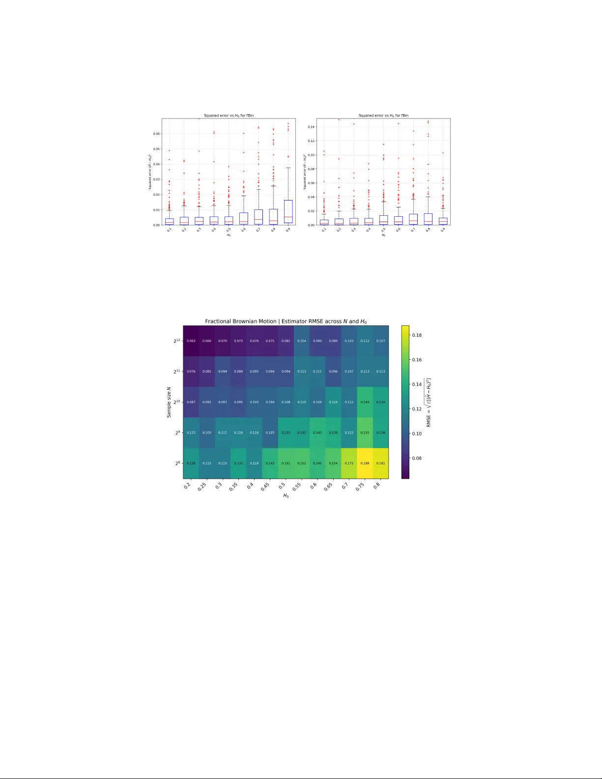
Estimation of the Self-similarit y Index of Non-stationary Incremen ts Self-similar Pro cesses via Lamp erti T ransformations William W u 1 and Qidi P eng 2 1 R ancho Cuc amonga High Scho ol, e-mail: wwu49387@gmail.com 2 Institute of Mathematic al Scienc es, Clar emont Gr aduate University, e-mail: * qidi.peng@cgu.edu Abstract: W e introduce a no vel method for estimating the self-similarity index of a general H -self-similar pro cess with either stationary or non- stationary increments. The estimation algorithm is developed based on a mo dified Lamp erti transformation, which transforms H -self-similar pro- cesses to stationary ones. As an application, we show how to use this ap- proach to estimate the self-similarity index of fractional Brownian motion, subfractional Brownian motion, bifractional Brownian motion, and trifrac- tional Bro wnian motion. Sim ulation study is p erformed to support the con- sistency of our estimators. Implementation in Python is publicly shared. Application on the estimation of the self-similarity index of the Nile river water level data from the year 900 to 1200 C.E.. MSC2020 sub ject classifications : Primary 60G18, 60G22; secondary 65C10. Keyw ords and phrases: Estimation, self-similarity index, Lamperti trans- formation, subfractional Brownian motion, bifractional Brownian motion, trifractional Brownian motion. 1. Literature Review on the Estimation of the Self-similarit y Index Self-similar pro cesses are stochastic pro cesses that exhibit the prop ert y of in- v ariance in distribution under scaling of time and space. These pro cesses are essen tial notions in sto chastic pro cesses and fractal geometry [ 18 ], with div erse applications in real-w orld fields suc h as pac k et inter-arriv al times and burst lengths [ 1 , 12 ], and global financial equit y markets [ 3 , 4 , 15 , 17 ]. Such pro cesses exhibit the phenomenon of “self-similarity” and are often asso ciated with the “rough path” feature: the pro cess’s sample path is mainly characterized b y its self-similarit y index. In this paper, w e consider the H -self-similar process defined b elo w: Definition 1.1 . W e say V = { V ( t ) } t ∈ R is an H -self-similar pro cess with self- similarit y index H ∈ (0 , 1), if { V ( at ) } t ∈ R f.d.d. =  | a | H V ( t )  t ∈ R , for an y real num b er a  = 0 , (1.1) 1 W. W u and Q. Peng/Estimation of the Self-similarity Index 2 where f.d.d. = denotes equality in finite dimensional distribution, i.e., for an y n ≥ 1 and any t 1 , . . . , t n ∈ R , ( V ( at 1 ) , . . . , V ( at n )) la w = | a | H ( V ( t 1 ) , . . . , V ( t n )) , for any real num b er a  = 0 . Concerning to estimate the self-similarit y index H of a H -self-similar process, there exist several metho d in the literature, how ever, each of them deals with a sp ecial case. Therefore, the goal of this pap er is to remedy this inconv enience b y dev eloping a general metho d to estimate the self-similarity index of a large class of fourth order H -self-similar processes. 2. A Mo dified Lamp erti T ransformation: A Nov el Estimation Approac h 2.1. L amp erti T r ansformation Our simulation approaches are inspired by the Lamp erti transformations. In 1962, Lamp erti in tro duced the Lamp erti transformation to transform H -self- similar processes to stationary pro cesses, and the inv erse operator do es so vice v ersa. The t wo transformations are defined as follo ws [ 10 ]. Definition 2.1 . Let { V ( t ) } t ∈ R b e an H -self-similar pro cess with self-similarit y index H ∈ (0 , 1), the Lamp erti transformation of { V ( t ) } t ∈ R is defined to b e L V ( t ) = e − tH V ( e t ) for t ∈ R . (2.1) Let { U ( t ) } t ∈ R b e a stationary sto chastic pro cess, i.e., for any integer n ≥ 1, any time indices t 1 , . . . , t n ∈ R and any time shifting parameter h > 0, w e ha ve ( U t 1 , . . . , U t n ) la w = ( U t 1 + h , . . . , U t n + h ) . F or eac h H ∈ (0 , 1), the inv erse Lamp erti transformation of { U ( t ) } t ∈ R is giv en b y L − 1 U (0) = 0; L − 1 U ( t ) = t H U (log t ) for t > 0 . Through the paper, w e assume that σ 2 = V ar ( V (1)) . (2.2) The main goal of this pap er is to provide a nov el and general metho d to esti- mate the self-similarity index of { V ( t ) } t ∈ [0 , 1] . The options of the metho dologies dep end on the situation for the cases for known σ and unknown σ . In Definition 2.1 , the fact that {L V ( t ) } t ∈ R is stationary inspires us to develop a nov el estima- tion strategy . Heuristically sp eaking, our metho d inv olves first transforming the H -self-similar pro cess to an ergo dic stationary one by using some mo dified Lam- p erti transformation, then running statistical estimation of the self-similarity index on the latter process. W. W u and Q. Peng/Estimation of the Self-similarity Index 3 2.2. Estimation of the Self-similarity Index When σ 2 is Given If σ 2 is known, w e assume that {L V ( t ) } t ∈ [0 , 1] is ergo dic. In view of the defini- tion of H -self-similar pro cess and the Lamp erti transformation, we suggest the follo wing w ay to estimate the self-similarit y index H of the process { V ( t ) } t ∈ [0 , 1] . Algorithm 2.2. Step 1 Define the se quenc es a = ( a 0 , . . . , a n ) and b = ( b 0 , . . . , b n ) : a =  V  ⌊ n j /n ⌋ n  j =0 ,...,n and b =  n 1 − j /n  j =0 ,...,n , (2.3) wher e ⌊•⌋ denotes the flo or numb er. Step 2 U se a non-line ar le ast squar es metho d to solve H fr om the e quation f n ( H ) := P n j =0 a 2 j b 2 H j n + 1 − σ 2 = 0 . (2.4) F or example, the solution b H c an b e solve d fr om Hal ley’s metho d [ 19 ]. Let us heuristically explain the rationales of Algorithm 2.2 . 1. In Step 1 , it is from the integer J n = ⌈− n log n ( n 1 /n − 1) ⌉ suc h that {⌊ n j /n ⌋} j ∈{ 0 ,...,n } are all distinct. In fact, J n is the smallest integer suc h that n ( j +1) /n − n j /n ≥ 1 for all j ≥ J n . 2. In Step 2 , w e ha ve used the fact that U n  j n  := L V  j n − 1  log( n )  = n − H ( j /n − 1) V ( n j /n − 1 ) for j ∈ { 0 , . . . , n } (2.5) is stationary and ergo dic. Therefore, P n j =0 V ( n j /n − 1 ) 2 n 2 H (1 − j /n ) n + 1 − V ar ( V (1)) P − − − − − → n → + ∞ 0 . (2.6) W e also hav e V  n j /n − 1  ≈ V  ⌊ n j /n ⌋ n  = a j a.s.. It results that P n j =0 a 2 j b 2 H j n + 1 − σ 2 P − − − − − → n → + ∞ 0 . (2.7) W. W u and Q. Peng/Estimation of the Self-similarity Index 4 2.3. Estimation of the Self-similarity Index When σ 2 is Unknown If σ 2 is unkno wn, we further assume that E ( V (1) 4 ) < + ∞ . W e then observe that b κ n ( H ) := ( n + 1) P n j =0 a 4 j b 4 H j  P n j =0 a 2 j b 2 H j  2 a.s. − − − − − → n → + ∞ E ( V (1) 4 ) ( E ( V (1) 2 )) 2 . b κ n ( H ) is then a consisten t estimator of the kurtosis of the stationary distribution V (1). This kurtosis is the measure of disp ersion of Z 2 around its exp ectation 1, where Z = V (1) 2 / p E ( V (1) 2 ). Therefore, the maximum likelihoo d estimation metho d is equiv alen t to minimizing the kurtosis via H , i.e., b H n := arg min H ∈ (0 , 1) b κ n ( H ) a.s. − − − − − → n → + ∞ H . W e then prop ose the follo wing algorithm: Algorithm 2.3. Step 1 Define the se quenc es a = ( a 0 , . . . , a n ) and b = ( b 0 , . . . , b n ) as in ( 2.3 ). Step 2 U se Br ent’s metho d [ 6 ] to solve the fol lowing optimization pr oblems b H n = arg min H ∈ (0 , 1) P n j =0 a 4 j b 4 H j  P n j =0 a 2 j b 2 H j  2 . (2.8) 3. Estimation of the Self-similarit y Index with Examples In this section, we will estimate and the self-similarity index for fractional Bro w- nian motion, subfractional Bro wnian motion, bifractional Brownian motion, and trifractional Brownian motion. 3.1. F r actional Br ownian motion The fractional Brownian motion { B H ( t ) } t ≥ 0 [ 14 ] with the Hurst parameter H ∈ (0 , 1) that w e consider in this framew ork is defined as a zero mean Gaussian pro cess with B H (0) = 0 a.s. and cov ariance function given b y: for s, t ≥ 0, γ B H ( s, t ) = σ 2 2  | t | 2 H + | s | 2 H − | t − s | 2 H  . (3.1) In a sim ulation study , we use our estimation for pro cesses sim ulated using W o o d Chan’s method [ 20 ]. Simulations and estimations were p erformed. W e generate 200 tra jectories of fBm with length N = 2 l for l ∈ { 7 , 8 , 9 , 10 } and H ∈ { 0 . 2 , 0 . 5 , 0 . 7 , 0 . 8 } . All of the follo wing results show the mean estimated H and the mean squared error in parentheses. S W. W u and Q. Peng/Estimation of the Self-similarity Index 5 T able 1 Estimator of H with MSE b ase d on fBm simulated by W o o d-Chan ’s Metho d: σ 2 = 1 H N = 128 N = 256 N = 512 N = 1024 0.2 0.237 (0.0213) 0.226 (0.0191) 0.220 (0.0121) 0.209 (0.0084) 0.5 0.538 (0.0524) 0.505 (0.0195) 0.508 (0.0149) 0.510 (0.0112) 0.7 0.733 (0.0715) 0.686 (0.0502) 0.715 (0.0211) 0.715 (0.0125) 0.8 0.823 (0.0916) 0.849 (0.0361) 0.809 (0.0238) 0.818 (0.0219) The following results are for Algorithm 2.3 where the self-similar scaling parameter is not known. T able 2 Estimator of H with MSE b ase d on fBm simulated by W o o d-Chan ’s Metho d: σ 2 is unknown H N = 128 N = 256 N = 512 N = 1024 N = 8192 0.2 0.286 (0.0405) 0.264 (0.0307) 0.235 (0.0205) 0.228 (0.0112) 0.219 (0.0067) 0.5 0.504 (0.0503) 0.504 (0.0311) 0.496 (0.0234) 0.515 (0.0203) 0.507 (0.0105) 0.7 0.668 (0.0350) 0.684 (0.0317) 0.683 (0.0255) 0.658 (0.0253) 0.691 (0.0113) 0.8 0.743 (0.0401) 0.721 (0.0466) 0.754 (0.0276) 0.753 (0.0245) 0.773 (0.0148) F or comparison, we can test the accuracy against the quadratic v ariation estimation metho d (QV estimator) [ 7 ] and the complex v ariation estimation metho d [ 9 ] b y running the same simu lations. The results are giv en below. T able 3 Quadr atic V ariation Estimator of H . H N = 128 N = 256 N = 512 N = 1024 0.2 0.193 (0.0056) 0.204 (0.0025) 0.207 (0.0012) 0.199 (0.0006) 0.5 0.499 (0.0072) 0.498 (0.0030) 0.499 (0.0015) 0.497 (0.0009) 0.7 0.683 (0.0080) 0.690 (0.0036) 0.702 (0.0021) 0.698 (0.0009) 0.8 0.794 (0.0088) 0.799 (0.0044) 0.797 (0.0020) 0.794 (0.0010) T able 4 Complex V ariations Estimator of H . H N = 128 N = 256 N = 512 0.5 0.500 (0.050) 0.500 (0.022) 0.490 (0.012) 0.7 0.680 (0.040) 0.690 (0.023) 0.710 (0.010) 0.8 0.825 (0.037) 0.805 (0.020) 0.800 (0.008) The comparison shows that our estimation metho ds are comp etitive to the literature ones for estimating the Hurst parameter of fractional Brownian mo- tion. A dditional visualization of the error analysis result is given b elow. W. W u and Q. Peng/Estimation of the Self-similarity Index 6 Fig 1 . The r esults ar e given by left: A lgorithm 2.2 , right: A lgorithm 2.3 . Each H 0 c onsists of 200 simulated paths of length N = 4096 . Square d err or of the estimate d p ar ameter is c ompute d for e ach p ath and dr awn into a b oxplot. Outliers over 99th per c entile ar e cut out for the sake of cle ar visuals. Fig 2 . 200 p aths of fBm ar e simulate d for e ach c orr esp onding H 0 and N value with the RMSE plotte d as a heatmap distribution. The r esults show empiric al c onver genc e towar ds 0 as the p ath length incre ases and H 0 value de cr e ases. The ab ov e figures show that in b oth cases, the ov erall p erformance of the estimation is consisten t. 3.2. Subfr actional Br ownian motion The subfractional Bro wnian motion { S H ( t ) } t ≥ 0 is defined to b e a zero-mean Gaussian process with S H (0) = 0 a.s. and co v ariance function (see [ 5 ]): for W. W u and Q. Peng/Estimation of the Self-similarity Index 7 s, t ≥ 0, C ov  S H ( t ) , S H ( s )  = σ 2  t 2 H + s 2 H − 1 2  ( t + s ) 2 H + | t − s | 2 H   , (3.2) where the parameter H ∈ (0 , 1). By ( 3.2 ), we know that { S H } t ≥ 0 is an H -self- similar pro cess. How ev er, unlike the fractional Brownian motion, the subfrac- tional Brownian motion has non-stationary incremen ts when H  = 1 / 2. This prop ert y makes its sim ulation quite challenging. The simulation approac h exist- ing in the literature is based on the DPW method pro vided in [ 16 ] with a v ailable co de in https://pypi.org/project/fractal- analysis/ . T o estimate H when σ 2 is known as 1, it suffices to note that σ 2 = V ar ( S H (1)) = 2 − 2 2 H − 1 . Mo difying a bit Algorithm 2.2 , w e obtain the algorithm to estimate H . Algorithm 3.1. L et ( S H ( j /n )) j =1 ,...,n b e an observe d sample p ath of { S H ( t ) } t ∈ [0 , 1] with c ovarianc e function γ S H with σ 2 = 1 . Step 1 L et the se quenc es a = ( a 0 , . . . , a n ) and b = ( b 0 , . . . , b n ) : a =  S H  ⌊ n j /n ⌋ n  j =0 ,...,n and b =  n 1 − j /n  j =0 ,...,n , wher e ⌊•⌋ denotes the flo or numb er. Step 2 U se a non-line ar le ast squar es metho d to solve H fr om the e quations f n ( H ) := P n j =0 a 2 j b 2 H j n + 1 − (2 − 2 2 H − 1 ) = 0 . W e show that our estimation metho ds p erform well for sfBm using the DPW sim ulation algorithm. W e generate 200 tra jectories of sfBm with length N = 2 l for l ∈ { 7 , 8 , 9 , 10 } and H ∈ { 0 . 2 , 0 . 5 , 0 . 7 , 0 . 8 } . The following results show the mean estimator H with the MSE in parentheses. T able 5 Subfr actional Br ownian motion: Algorithm 3.1 H N = 128 N = 256 N = 512 N = 1024 0.2 0.228 (0.0218) 0.216 (0.0128) 0.228 (0.0090) 0.214 (0.0071) 0.5 0.509 (0.0142) 0.509 (0.0107) 0.508 (0.0077) 0.508 (0.0060) 0.7 0.695 (0.0081) 0.703 (0.0066) 0.702 (0.0052) 0.705 (0.0044) 0.8 0.785 (0.0061) 0.799 (0.0051) 0.799 (0.0033) 0.801 (0.0027) The simulation results for algorithm 2.3 is given b elow: W. W u and Q. Peng/Estimation of the Self-similarity Index 8 T able 6 Subfr actional Br ownian motion: Algorithm 2.3 H N = 128 N = 256 N = 512 N = 1024 N = 8192 0.2 0.251 (0.0370) 0.266 (0.0272) 0.250 (0.0274) 0.247 (0.0191) 0.220 (0.0086) 0.5 0.500 (0.0388) 0.501 (0.0293) 0.516 (0.0227) 0.500 (0.0153) 0.500 (0.0096) 0.7 0.635 (0.0494) 0.657 (0.0273) 0.661 (0.0263) 0.668 (0.0240) 0.680 (0.0109) 0.8 0.750 (0.0351) 0.761 (0.0314) 0.762 (0.0268) 0.732 (0.0291) 0.762 (0.0171) A dditional data visualization is given. Fig 3 . The r esults ar e given by left: A lgorithm 2.2 , right: A lgorithm 2.3 . Each H 0 c onsists of 200 simulated paths of length N = 4096 . Square d err or of the estimate d p ar ameter is c ompute d for e ach p ath and dr awn into a b oxplot. Outliers over 99th per c entile ar e cut out for the sake of cle ar visuals. W. W u and Q. Peng/Estimation of the Self-similarity Index 9 Fig 4 . 200 p aths of sfBm are simulate d for e ach c orresp onding H 0 and N value with the RMSE plotte d as a heatmap distribution. The r esults show empiric al c onver genc e towar ds 0 as the p ath length incr e ases. 3.3. Bifr actional Br ownian motion The bifractional Bro wnian motion { B H,K ( t ) } t ≥ 0 is a zero-mean Gaussian pro- cess with B H,K (0) = 0 a.s. and cov ariance function (see [ 8 ]): for s, t ≥ 0, C ov  B H,K ( t ) , B H,K ( s )  = σ 2 2 K  ( t 2 H + s 2 H ) K − | t − s | 2 H K  , (3.3) where the parameters H ∈ (0 , 1) and K ∈ (0 , 1]. By ( 3.3 ), we see that { B H,K ( t ) } t ≥ 0 is an H K -self-similar pro cess. When K = 1, { B H, 1 ( t ) } t ≥ 0 b ecomes a fractional Bro wnian motion with the Hurst parameter H . F or K < 1, the bifractional Bro wnian motion do es not hav e stationary incremen ts. T o estimate the self- similarit y H K , it suffices to apply Algorithm 2.2 and Algorithm 2.3 . Note that the simulation metho d is also provided in the DPW metho d [ 16 ]. The follo wing table sho ws our estimation metho d for bfBm using the DPW sim ulation algorithm. Like before, w e will generate 200 tra jectories of bfBm with lengths N = 128 , 256 , 512 , 1024. This will b e tested on paths with ( H , K ) ∈ ( { 0 . 2 , 0 . 8 } , { 0 . 5 , 0 . 8 } ) to estimate the self-similarity v alue H K . T able 7 Bifr actional Br ownian motion: Algorithm 2.2 with σ 2 = 1 ( H, K ) N = 128 N = 256 N = 512 N = 1024 (0.2, 0.5) 0.108 (0.0074) 0.107 (0.0058) 0.114 (0.0044) 0.111 (0.0026) (0.2, 0.8) 0.174 (0.0207) 0.172 (0.0106) 0.172 (0.0072) 0.175 (0.0051) (0.8, 0.5) 0.391 (0.0131) 0.418 (0.0124) 0.399 (0.0075) 0.404 (0.0042) (0.8, 0.8) 0.650 (0.0344) 0.654 (0.0186) 0.635 (0.0151) 0.654 (0.0079) W. W u and Q. Peng/Estimation of the Self-similarity Index 10 The results for Algorithm 2.3 when the scaling parameter is not kno wn is giv en b elow. T able 8 Bifr actional Br ownian motion: Algorithm 2.3 with unknown σ 2 ( H, K ) N = 128 N = 256 N = 512 N = 1024 N = 8192 (0 . 2 , 0 . 5) 0.230 (0.0627) 0.200 (0.0428) 0.161 (0.0192) 0.149 (0.0139) 0.122 (0.0058) (0 . 8 , 0 . 5) 0.431 (0.0280) 0.422 (0.0301) 0.417 (0.0196) 0.411 (0.0130) 0.411 (0.0070) (0 . 2 , 0 . 8) 0.266 (0.0558) 0.235 (0.0332) 0.212 (0.0200) 0.199 (0.0112) 0.186 (0.0081) (0 . 8 , 0 . 8) 0.639 (0.0317) 0.616 (0.0287) 0.625 (0.0245) 0.607 (0.0174) 0.619 (0.0094) Lik e b efore, the data visualization is given. Fig 5 . The r esults ar e given by left: A lgorithm 2.2 , right: A lgorithm 2.3 . Each H 0 c onsists of 200 simulated paths of length N = 4096 . Square d err or of the estimate d p ar ameter is c ompute d for e ach p ath and dr awn into a b oxplot. Outliers over 99th per c entile ar e cut out for the sake of cle ar visuals. 3.4. T rifr actional Br ownian Motion Another example of Gaussian pro cesses with non-stationary incremen ts is the trifractional Brownian motion { e B H,K ( t ) } t ≥ 0 [ 13 ]. It is a zero-mean Gaussian pro cess with e B H,K (0) = 0 a.s. and cov ariance function: for s, t ≥ 0, C ov  e B H,K ( t ) , e B H,K ( s )  = σ 2  t 2 H K + s 2 H K −  t 2 H + s 2 H  K  , (3.4) where the parameters H ∈ (0 , 1) and K ∈ (0 , 1). F rom its definition, w e see that { e B H,K ( t ) } t ≥ 0 is H K -self-similar, and its increment processes are not stationary . Lik e the bifractional Bro wnian motion, this pro cess also cannot b e simulated using the sum of stationary increments. So far as we kno w, the only simulation approac h suggested in the literature is the DPW metho d. When σ 2 = 1, the esti- mation of the self-similarity index H K is then obtained by a slight modification of Algorithm 2.2 : Algorithm 3.2. L et ( e B H,K ( j /n )) j =1 ,...,n b e an observe d sample p ath of { e B H,K ( t ) } t ∈ [0 , 1] with c ovarianc e function γ e B H,K . W. W u and Q. Peng/Estimation of the Self-similarity Index 11 Step 1 L et the se quenc es a = ( a 0 , . . . , a n ) and b = ( b 0 , . . . , b n ) : a =  e B H,K  ⌊ n j /n ⌋ n  j =0 ,...,n and b =  n 1 − j /n  j =0 ,...,n , wher e ⌊•⌋ denotes the flo or numb er. Step 2 U se a non-line ar le ast squar es metho d to solve H , K fr om the e quations f n ( H , K ) := P n j =0 a 2 j b 2 H K j n + 1 − (2 − 2 K ) = 0 . Lik e bifractional Brownian motion, the same parameters for testing are ap- plied to tfBm simulated b y the DPW algorithm. The results are given b elow: T able 9 T rifr actional Br ownian motion: A lgorithm 3.2 . ( H, K ) N = 128 N = 256 N = 512 N = 1024 (0.2, 0.5) 0.203 (0.1038) 0.161 (0.0700) 0.170 (0.0549) 0.171 (0.0442) (0.2, 0.8) 0.263 (0.0904) 0.263 (0.0603) 0.212 (0.0555) 0.212 (0.0312) (0.8, 0.5) 0.442 (0.0672) 0.461 (0.0460) 0.427 (0.0319) 0.448 (0.0195) (0.8, 0.8) 0.659 (0.0520) 0.655 (0.0327) 0.549 (0.0293) 0.656 (0.0188) Finally the results for trifractional Brownian motion when the scaling pa- rameter is not known, giv en b y Algorithm 2.3 , is given b elow. T able 10 T rifr actional Br ownian motion: A lgorithm 2.3 ( H, K ) N = 128 N = 256 N = 512 N = 1024 N = 8192 (0 . 2 , 0 . 5) 0.134 (0.0194) 0.140 (0.0210) 0.136 (0.0236) 0.130 (0.0163) 0.121 (0.0094) (0 . 8 , 0 . 5) 0.384 (0.0414) 0.421 (0.0375) 0.408 (0.0399) 0.406 (0.0303) 0.405 (0.0185) (0 . 2 , 0 . 8) 0.212 (0.0367) 0.182 (0.0220) 0.193 (0.0218) 0.179 (0.0173) 0.172 (0.0144) (0 . 8 , 0 . 8) 0.616 (0.0434) 0.626 (0.0379) 0.628 (0.0412) 0.642 (0.0299) 0.628 (0.0194) The error analysis result is illustrated b elow: Fig 6 . The r esults ar e given by left: A lgorithm 2.2 , right: A lgorithm 2.3 . Each H 0 c onsists of 200 simulated paths of length N = 4096 . Square d err or of the estimate d p ar ameter is c ompute d for e ach p ath and dr awn into a b oxplot. Outliers over 99th per c entile ar e cut out for the sake of cle ar visuals. W. W u and Q. Peng/Estimation of the Self-similarity Index 12 W e conclude that: (1) Our estimation metho d is comp etitive to the literature ones for estimation of the Hurst parameter of fractional Brownian motion. (2) Our estimation fills the gaps when the target process has non-stationary incremen ts. This makes our metho d b e able to estimate the self-similarity indexes of sub-fBm, bifBm, and trifBm. 3.5. Co de availability In this section, we list the codes for all methods men tioned in this pap er. Among them, we hav e contributed the following: • Estimation pro cess to obtain comparison data (Python): https://github. com/william11074/Self- similar- Statistical- Inference • Simulation algorithm for fBm, sfBm, bfBm, and tfBm using b oth W oo d Chan’s metho d and DPW metho d, along with implementation of the QV metho d: pip install fractal-analysis: https://pypi.org/project/fractal- analysis/ 4. Real W orld Application: The Nile Riv er Studies conducted b y Bardet [ 2 ] and Lee et. al [ 11 ] show that the annual min- im um water levels of the Nile River are self-similar with the prop ert y of long- range dependency . These papers detail that the self-similarit y index of the ob- serv ed water levels b etw een y ears 722 and 1281 match H ≈ 0 . 88. W e take the interv al from the year 900 to 1200 for the Nile River data and using Algorithm 2.3 , we get a predicted H v alue of 0 . 8545. How ever, apply- ing parametric b o otstrap bias correction, the corrected v alue H B C = 0 . 8790, matc hing the results in literature. Op en source data is used from http://lib. stat.cmu.edu/S/beran . W. W u and Q. Peng/Estimation of the Self-similarity Index 13 Fig 7 . Plotte d is the available dataset of annual Nile R iver data fr om ye ars 622-1284 C.E. The ye ars 900-1200 is chosen for the estimation of the self-similarity index. 5. Conclusion This pap er develops a general wa y to estimate the self-similarity index for a giv en second-order self-similar sto chastic pro cess that is ergo dic with emphasis that the method works for non-stationary incremen ts self-similar processes. T wo estimation algorithms are given for when the scaling parameter is known or un- kno wn. Sim ulation and testing sho w that results are accurate and comparable to other methods in the literature. In addition, application to real-w orld data, the NIle River’s historical water level, shows use cases. GitHub co de is do cumented and provided for the estimation algorithms. References [1] Abr y, P. , Flandrin, P. , T a qqu, M. S. and Veitch, D. (2000). W av elets for the analysis, estimation, and synthesis of scaling data. Self-similar Net- work T r affic and Performanc e Evaluation 39–88. [2] Bardet, J.-M. (2000). T esting for the presence of self-similarity of Gaus- sian time series ha ving stationary incremen ts. Journal of Time Series A nal- ysis 21 497–515. [3] Bianchi, S. , P ant anella, A. and Pianese, A. (2012). Mo deling and sim ulation of currency exchange rates using multifractional process with random exp onent. International Journal of Mo deling and Optimization 2 309. W. W u and Q. Peng/Estimation of the Self-similarity Index 14 [4] Bianchi, S. and Pianese, A. (2008). Multifractional prop erties of sto ck indices decomp osed by filtering their p oin t wise H¨ older regularity . Interna- tional Journal of The or etic al and A pplie d Financ e 11 567–595. [5] Bojdecki, T. , Gorostiza, L. G. and T alar czyk, A. (2004). Sub- fractional Bro wnian motion and its relation to o ccupation times. Statistics & Pr ob ability L etters 69 405–419. [6] Brent, R. P. (1971). An algorithm with guaranteed con vergence for find- ing a zero of a function. The c omputer journal 14 422–425. [7] Coeurjoll y, J.-F. (2005). Iden tification of multifractional Bro wnian mo- tion. Bernoul li 11 987–1008. [8] Houdr ´ e, C. and Villa, J. (2003). An example of infinite dimensional quasi-helix. Contemp or ary Mathematics 336 195–202. [9] Ist as, J. (2012). Estimating self-similarity through complex v ariations. Ele ctr onic Journal of Statistics 6 1392–1408. [10] Lamper ti, J. (1962). Semi-stable sto chastic processes. T r ansactions of the A meric an Mathematic al So ciety 104 62–78. [11] Lee, M. , Genton, M. G. and Jun, M. (2016). T esting self-similarity through Lamperti transformations. Journal of agricultur al, biolo gic al, and envir onmental statistics 21 426–447. [12] Leland, W. E. , T aqqu, M. S. , Willinger, W. and Wilson, D. V. (1994). On the self-similar nature of Ethernet traffic (extended version). IEEE/A CM T r ansactions on Networking 2 1-15. [13] Ma, C. (2013). The Sc ho enberg–Le´ evy kernel and relationships among fractional Brownian motion, bifractional Bro wnian motion, and others. The ory of Pr ob ability & its A pplic ations 57 619–632. [14] Mandelbrot, B. and v an Ness, J. W. (1968). F ractional Brownian mo- tions, fractional noises and applications. SIAM R eview 10 422–437. [15] Peng, Q. (2011). Inf ´ erence statistique p our des pro cessus multifraction- naires cach ´ es dans un cadre de mo d` eles ` a volatilit ´ e sto chastique, PhD thesis, PhD thesis, Univ ersit´ e des Sciences et T echnologies de Lille. [16] Peng, Q. and Wu, W. (2025). In vestigation and Dev elopment of the Metho dologies for Simulating Self-similar Pro cesses. arXiv pr eprint arXiv:2512.07296 . [17] Peng, Q. and Zhao, R. (2019). A general class of multifractional pro cesses and sto ck price informativeness. Chaos, Solitions & F r actals 115 248-267. [18] Samorodnitsky, G. and T a qqu, M. S. (1994). Stable Non-Gaussian R andom Pr o c esses: Sto chastic Mo dels with Infinite V arianc e . Chapman & Hall, New Y ork. [19] Sca vo, T. R. and Thoo, J. B. (1995). On the Geometry of Halley’s Metho d. The A meric an Mathematic al Monthly 102 417–426. [20] Wood, A. T. A. and Chan, G. (1994). Sim ulation of stationary Gaussian pro cesses in [0 , 1] d . Journal of Computational and Gr aphic al Statistics 3 409–432.