Adaptive Penalized Doubly Robust Regression for Longitudinal Data

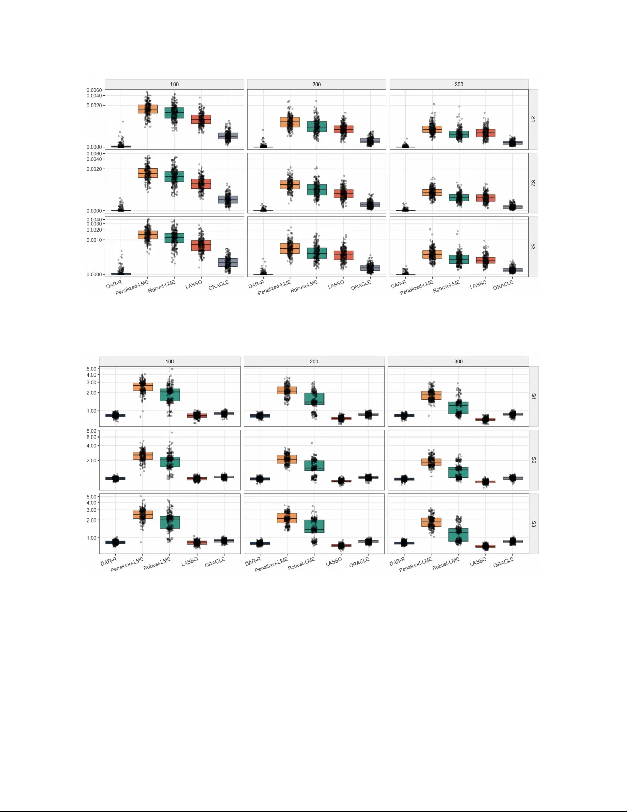
Adaptiv e P enalized Doubly Robust Regression for Longitudinal Data Y uy ao W ang 1 , Y u Lu 1 , Tianni Zhang 1 , Mengfei Ran ∗ 1 1 Wisdom Lake Academy of Pharmacy , Xi’an Jiaotong-Liverpo ol Universit y Abstract Longitudinal data often inv olve heterogeneit y , sparse signals, and contamination from re- sp onse outliers or high-leverage observ ations esp ecially in biomedical science. Existing metho ds usually address only part of this problem, either emphasizing p enalized mixed-eﬀects mo del- ing without robustness or robust mixed-eﬀects estimation without high-dimensional v ariable selection. W e prop ose a doubly adaptive robust regression (DAR-R) framew ork for longitu- dinal linear mixed-eﬀects models. It combines a robust pilot ﬁt, doubly adaptiv e observ ation w eigh ts for residual outliers and leverage p oin ts, and folded-concav e p enalization for ﬁxed-eﬀect selection, together with w eigh ted up dates of random eﬀects and v ariance comp onen ts. W e de- v elop an iterative rew eighting algorithm and establish estimation and prediction error b ounds, supp ort recov ery consistency , and oracle-type asymptotic normality . Sim ulations show that D AR-R impro ves estimation accuracy , false-positive control, and co v ariance estimation under b oth vertical outliers and bad leverage contamination. In the T ADPOLE/ADNI Alzheimer’s disease application, D AR-R achiev es accurate and stable prediction of AD AS13 while selecting clinically meaningful predictors with strong resampling stability . 1 In tro duction Longitudinal and clustered data arise routinely in biomedical researc h, economics, and the so cial sciences, where sub jects are measured rep eatedly o v er time and the resulting within-sub ject corre- lation m ust b e accoun ted for in v alid inference and eﬃcient prediction. Linear mixed-eﬀects mo dels (LMMs) provide a ﬂexible and widely used framew ork b y combining p opulation-lev el ﬁxed eﬀects with sub ject-sp eciﬁc random eﬀects; the foundational form ulation for longitudinal data was dev el- op ed by Laird and W are ( 1982 ). Comprehensiv e treatments and mainstream implemen tations are no w standard in longitudinal analysis ( Pinheiro and Bates , 2000 ; V erb ek e and Molenberghs , 2000 ; Diggle et al. , 2002 ), with widely used soft ware such as lme4 described by Bates et al. ( 2015 ). A t the same time, mo dern longitudinal studies often collect a large num b er of candidate predictors, making v ariable selection for mixed mo dels an essential comp onen t of scientiﬁc disco v ery . A growing literature addresses sparse estimation and v ariable selection for mixed-eﬀects mo dels through p enalized likelihoo d and related regularization strategies. Early w ork considers join t selec- tion of ﬁxed and random eﬀects ( Bondell et al. , 2010 ; Ibrahim et al. , 2011 ). In the high-dimensional regime, ℓ 1 -regularized estimators for LMMs hav e been analyzed with prov able guaran tees ( Sc hell- dorfer et al. , 2011 ). Despite these adv ances, most existing procedures are primarily dev elop ed ∗ Corresp onding author. mengfei.ran@xjtlu.edu.cn 1 under clean-data assumptions and ma y lose stability or selection accuracy when resp onse outliers or cov ariate leverage p oin ts are present. In practice, longitudinal data are frequently corrupted by outliers in responses (e.g., sp oradic assa y failures, recording errors) and by leverage p oin ts in co v ariates (e.g., data entry mistakes, device miscalibration, atypical cov ariate conﬁgurations). Robust statistics pro vides classical to ols for do wn weigh ting ab erran t observ ations ( Hub er , 1964 ; Hamp el et al. , 1986 ; Hub er and Ronchetti , 2009 ), and robust mixed-mo del pro cedures ha ve b een explored through heavy-tailed modeling and robust lik eliho o d/estimating-equation approac hes. F or instance, robust REML-type ideas for mixed mo dels w ere in vestigated by Richardson and W elsh ( 1995 ), and t -based robustiﬁcation for mixed- eﬀects mo dels was studied by Pinheiro et al. ( 2001 ). Nev ertheless, most existing robust mixed- mo del metho ds fo cus on low-dimensional settings, and do not directly address high-dimensional v ariable selection with sim ultaneous protection against resp onse outliers and co v ariate leverage p oin ts ( Koller , 2016 ). Relatedly , Ran and Xu ( 2024 ) proposed robust v ariable selection via noncon- ca ve p enalties with an upgraded parsimonious dynamic co v ariance mo deling, highlighting the v alue of com bining robustness, dep endence mo deling, and sparsity in correlated-data settings. Here w e use the term doubly robust in the outlier-robustness sense, emphasizing protection against b oth resp onse con tamination and cov ariate lev erage (not the causal-inference meaning). This paper develops an adaptiv e p enalized doubly robust regression framework for longitudinal analysis under high-dimensionality , termed longitudinal DAR-R. The metho d integrates three in- gredien ts. First, robust pilot ﬁts deliver reliable residuals and scale estimates that serve as anchors for calibration. Second, D AR-R assigns observ ation-sp eciﬁc w eights that reﬂect t wo complemen- tary notions of outlyingness: one comp onen t do wnw eights large standardized residuals, while the other targets cov ariate leverage through robust distance measures ( Rousseeuw and Leroy , 1987 ; Rousseeu w and V an Driessen , 1999 ). These tw o comp onen ts are linked by a global discrepancy factor that adapts the o v erall aggressiv eness of down weigh ting to the con tamination lev el in the data, so the procedure remains eﬃcient for clean samples y et protectiv e under severe contamina- tion. Third, after weigh ting, ﬁxed eﬀects are estimated using folded-concav e regularization: F an and Li ( 2001 ) established the oracle-prop ert y viewpoint for nonconca ve p enalties, and Zhang ( 2010 ) prop osed the MCP family . Random eﬀects and v ariance components are then up dated through a w eighted empirical Bay es/REML step, leading to a stable iterativ e rew eigh ting algorithm. The the- oretical analysis builds on the ge n eral M-estimation framework of Negahban et al. ( 2012 ) together with mo dern results for nonconv ex regularization ( Loh and W ainwrigh t , 2015 ; W ainwrigh t , 2019 ). Our main con tributions are as follows. W e introduce longitudinal DAR-R, a robust-and-sparse framew ork for high-dimensional LMMs that simultaneously protects against response outliers and co v ariate leverage through doubly adaptive weigh ting with a data-adaptive discrepancy factor. W e also pro vide a practical and scalable implemen tation via an iterative reweigh ting algorithm that couples w eigh ted empirical Ba y es/REML up dates for random eﬀects and v ariance comp onen ts with co ordinate-descen t style updates for folded-conca ve p enalization ( Breheny and Huang , 2011 ). On the theoretical side, w e establish nonasymptotic b ounds for estimation and prediction, and further sho w consisten t supp ort reco very and oracle asymptotic normalit y under suitable regularit y conditions. Finally , extensive simulations and an application study illustrate that D AR-R achiev es impro ved robustness and v ariable-selection accuracy relative to existing p enalized mixed-mo del comp etitors, particularly under mixed contamination scenarios. The rest of the pap er is organized as follows. Section 2 presen ts the longitudinal DAR-R mo del form ulation and the doubly adaptiv e weigh ting scheme. Section 3 describ es the computational pro cedure and iterativ e reweigh ting algorithm. Section 4 establishes the theoretical prop erties of the prop osed estimator. Section 5 rep orts simulation studies, and Section 6 provides a real-data application to the T ADPOLE/ADNI longitudinal Alzheimer’s disease cohort. Section 7 concludes 2 with a summary and future directions. 2 Metho dology 2.1 Mo del Sp eciﬁcation F or sub jects i = 1 , . . . , n and times t = 1 , . . . , T i , let Y it ∈ R denote the outcome, with ﬁxed-eﬀect co v ariates X it ∈ R p and random-eﬀect cov ariates Z it ∈ R q . W e consider the longitudinal linear mixed-eﬀects mo del Y it = X ⊤ it β ⋆ + Z ⊤ it b i + ε it , (1) where β ⋆ ∈ R p is the unknown ﬁxed-eﬀect v ector of in terest, b i ∈ R q is a sub ject-sp eciﬁc random eﬀect, and ε it is the idiosyncratic noise. W e assume E ( b i ) = 0 and Cov( b i ) = D ⋆ , while E ( ε it ) = 0 and V ar( ε it ) = ( σ ⋆ ) 2 , with indep endence across sub jects and ( i, t ) conditional on ( X it , Z it ). The within-sub ject dep endence is captured through the shared random eﬀect b i , follo wing the standard mixed-mo del form ulation; see, e.g., ( Laird and W are , 1982 ; V erbeke and Molen b erghs , 2000 ; Diggle et al. , 2002 ). F or compact notation, deﬁne the stack ed resp onse and design matrices Y i = ( Y i 1 , . . . , Y iT i ) ⊤ , X i =  X i 1 , . . . , X iT i  ⊤ ∈ R T i × p and Z i =  Z i 1 , . . . , Z iT i  ⊤ ∈ R T i × q , so that Y i = X i β ⋆ + Z i b i + ε i . Let N = P n i =1 T i b e the total num b er of observ ations. Our primary goal is estimation and v ariable selection for β ⋆ when p can b e comparable to or muc h larger than N . W e assume β ⋆ is sparse with supp ort S = { j : β ⋆ j  = 0 } satisfying | S | = s ≪ p . 2.2 Doubly Adaptiv e Ob jectiv e P enalized mixed-mo del estimation can b e sensitive to contamination b ecause atypical observ ations ma y appear either as ab erran t responses (large residuals) or as co v ariate leverage p oin ts (extreme X -proﬁles). Our strategy is to build observ ation-sp eciﬁc w eights that do wnw eigh t both sources of con tamination, while automatically adapting the ov erall strength of do wnw eighting to the “clean- liness” of the dataset. Let ( ˜ β , { ˜ b i } , ˜ σ ) b e robust pilot estimates for the mixed mo del. Suc h pilots can b e obtained via ro- bust REML-t yp e ideas ( Ric hardson and W elsh , 1995 ), t -based robustiﬁcation ( Pinheiro et al. , 2001 ; Lange et al. , 1989 ), or practical robust mixed-mo del implementations ( Koller , 2016 ). T o assess co- v ariate leverage robustly , we also compute a robust lo cation–scatter pair ( ˜ ℓ, ˜ Σ) for { X it } , for exam- ple using the Minimum Cov ariance Determinant (MCD) estimator ( Rousseeuw and V an Driessen , 1999 ), which is standard in robust outlier detection ( Rousseeu w and Leroy , 1987 ; Maronna et al. , 2006 ). Based on the pilot ﬁt, w e quantify resp onse outlyingness by the standardized residual ˜ r it = Y it − X ⊤ it ˜ β − Z ⊤ it ˜ b i ˜ σ , so that unusually large | ˜ r it | indicates an ab erran t outcome relativ e to the ﬁtted mixed mo del. In parallel, w e measure cov ariate leverage using a robust Mahalanobis-t yp e distance computed from ( ˜ ℓ, ˜ Σ), d 2 ( X it ) = ( X it − ˜ ℓ ) ⊤ ˜ Σ − 1 ( X it − ˜ ℓ ) , where larger v alues corresp ond to atypical cov ariate proﬁles in the ﬁxed-eﬀect design space. Here ˜ ℓ ∈ R p denotes a robust estimate of the lo cation (cen ter) of the co v ariate vector X it , paired with a robust scatter estimate ˜ Σ (e.g., from MCD). 3 T o adapt the aggressiveness of down w eigh ting to the o veral l con tamination lev el, w e introduce a global discrepancy factor based on the empirical distribution of | ˜ r it | . Let F + n ( u ) = 1 N n X i =1 T i X t =1 1 ( | ˜ r it | ≤ u ) , F + 0 ( u ) = P ( | Z | ≤ u ) , Z ∼ N (0 , 1) , and deﬁne ˜ δ = sup u ≥ 0   F + n ( u ) − F + 0 ( u )   . In tuitively , ˜ δ is small when standardized residuals b eha ve close to the nominal reference, and b ecomes larger when the residual distribution exhibits noticeable tail inﬂation or distortion; it therefore calibrates ho w aggressively the procedure should down weigh t. If a diﬀeren t nominal error shap e is more appropriate, F + 0 can b e replaced accordingly without c hanging the rest of the construction. W e then deﬁne doubly adaptive weigh ts w it ∈ [0 , 1] as w it = ϕ 1  ˜ δ | ˜ r it |  · ϕ 2  ˜ δ d 2 ( X it )  , (2) where ϕ 1 , ϕ 2 : [0 , ∞ ) → [0 , 1] are non-increasing functions with ϕ k (0) = 1 and ϕ k ( u ) → 0 as u → ∞ . This form follows the b ounded-inﬂuence spirit of robust M-estimation ( Hub er , 1964 ; Hamp el et al. , 1986 ; Hub er and Ronchetti , 2009 ), while explicitly separating resp onse outlyingness and cov ariate lev erage. Practically , tw o con venien t choices are Hub er-t yp e weigh t ϕ ( u ) = min(1 , c/u ) and T ukey bisquare w eight ϕ ( u ) = { 1 − ( u/c ) 2 } 2 1 ( u ≤ c ); b oth yield w it ≈ 1 for t ypical observ ations and substan tially smaller weigh ts for extreme residuals and/or leverage p oin ts. Giv en weigh ts, we up date the random eﬀects using a robust empirical Bay es (REB) step: ˆ b i ( β ) = arg min b ∈ R q n T i X t =1 w it  Y it − X ⊤ it β − Z ⊤ it b  2 + b ⊤ ˆ D − 1 b o , (3) where ˆ D is a robust estimate of the random-eﬀect cov ariance. Denote W i = diag ( w i 1 , . . . , w iT i ), the solution has the closed form ˆ b i ( β ) = ( Z ⊤ i W i Z i + ˆ D − 1 ) − 1 Z ⊤ i W i ( Y i − X i β ) . Finally , w e estimate the ﬁxed eﬀect β by minimizing the weigh ted p enalized criterion ˆ β = arg min β ∈ R p    n X i =1 T i X t =1 w it  Y it − X ⊤ it β − Z ⊤ it ˆ b i ( β )  2 + N p X j =1 p λ ( | β j | )    , (4) where p λ ( · ) is a sparsity-inducing p enalt y . W e fo cus on folded-concav e p enalties suc h as SCAD and MCP , b ecause F an and Li ( 2001 ) established their oracle-t yp e b eha vior and Zhang ( 2010 ) prop osed the MCP family , b oth of which help reduce shrink age bias on strong signals compared to conv ex ℓ 1 p enalties. Computational details for optimizing ( 4 ) and up dating ( ˆ D , ˆ σ ) are deferred to Section 3 . 3 Computation The optimization problem in ( 4 ) is inheren tly coupled across m ultiple lay ers of unknowns, so a one-shot minimization is not practical. The ﬁxed eﬀects β determine ﬁtted v alues and hence 4 the standardized residuals that enter the doubly adaptive w eigh ts w it ; given these weigh ts, the random eﬀects ˆ b i ( β ) dep end on β through the weigh ted REB up date ( 3 ); and the weigh ts are then recalibrated from the curren t ﬁt through the residual- and leverage-based outlyingness measures. In addition, the v ariance comp onen ts ( D , σ 2 ) are naturally tied to the curren t estimates of { b i } and the weigh ted residual scale. This circular dep endence suggests an alternating pro cedure that rep eatedly up dates auxiliary quantities such as w eights, random eﬀects, and v ariance comp onen ts giv en the curren t β , and up dates β b y solving a weigh ted p enalized subproblem with those auxiliary quan tities held ﬁxed. The resulting scheme can b e interpreted as an EM-/ECM-t yp e approach ( Dempster et al. , 1977 ; Meng and Rubin , 1993 ) combined with an iterative reweigh ting (IRLS) viewp oin t: each iteration refreshes the data-adaptiv e weigh ts to attenuate resp onse outliers and co v ariate lev erage p oin ts, and then p erforms a stabilized p enalized mixed-mo del up date under the refreshed weigh ts. W e alternate b et ween an E-step, where we up date the unobserv ed comp onen ts (w eigh ts and random eﬀects) given the curren t parameters, and an M-step, where we up date the parameters ( β ) giv en the current weigh ts and random eﬀects. 3.1 EM Algorithm W e implemen t the prop osed estimator via an EM-st yle iterativ e rew eighting procedure. At iteration k , supp ose w e ha ve current estimates ( ˜ β ( k ) , ˜ D ( k ) , ˜ σ ( k ) ). The next iterate is obtained by an E-step that refreshes the w eights and random eﬀects (and up dates v ariance comp onen ts accordingly), follo wed by an M-step that up dates β under the new weigh ts. 3.1.1 E-step: Up dating W eigh ts and Random Eﬀects The E-step up dates all comp onen ts that are treated as laten t or auxiliary in the w eighted form u- lation. Using the current iterate ( ˜ β ( k ) , ˜ D ( k ) , ˜ σ ( k ) ), we p erform: Step 1-Up date W eigh ts: Compute standardized residuals based on the curren t ﬁt, ˜ r ( k ) it = Y it − X ⊤ it ˜ β ( k ) − Z ⊤ it ˜ b ( k ) i ˜ σ ( k ) , together with the robust leverage score d 2 ( X it ) in Section 2 . Then ev aluate the global discrepancy factor ˜ δ ( k ) and up date the observ ation weigh ts by w ( k +1) it = ϕ 1  ˜ δ ( k ) | ˜ r ( k ) it |  · ϕ 2  ˜ δ ( k ) d 2 ( X it )  , whic h is exactly the w eighting rule in ( 2 ). Intuitiv ely , w ( k +1) it iden tiﬁes and do wnw eigh ts observ a- tions that are currently assessed as resp onse outliers and/or leverage p oin ts. Step 2-Up date Random Eﬀects and V ariance Comp onen ts: Given w ( k +1) it , up date the random eﬀects by the weigh ted REB step ( 3 ): ˆ b ( k +1) i ( β ) =  Z ⊤ i W ( k +1) i Z i + ( ˜ D ( k ) ) − 1  − 1 Z ⊤ i W ( k +1) i ( Y i − X i β ) , W ( k +1) i = diag( w ( k +1) i 1 , . . . , w ( k +1) iT i ) . In practice, we plug in β = ˜ β ( k ) to obtain ˆ b ( k +1) i = ˆ b ( k +1) i ( ˜ β ( k ) ), and deﬁne the asso ciated p osterior co v ariance V ( k +1) i =  Z ⊤ i W ( k +1) i Z i + ( ˜ D ( k ) ) − 1  − 1 . 5 W e then up date the v ariance comp onen ts using the follo wing EM-type moment up dates: ˜ D ( k +1) = 1 n n X i =1 n ˆ b ( k +1) i ˆ b ( k +1) ⊤ i + V ( k +1) i o , (5) and ˜ σ 2( k +1) = 1 N n X i =1 n ∥ ( W ( k +1) i ) 1 / 2 e ( k +1) i ∥ 2 2 + T r  W ( k +1) i Z i V ( k +1) i Z ⊤ i  o , (6) where e ( k +1) i = Y i − X i ˜ β ( k ) − Z i ˆ b ( k +1) i . These up dates yield refreshed quantities ( ˜ D ( k +1) , ˜ σ 2( k +1) ) to b e used in the subsequent M-step. 3.1.2 M-step: Up dating Fixed Eﬀects ( β ) Conditioning on the up dated weigh ts w ( k +1) it and the refreshed v ariance comp onen ts, the M-step up dates the ﬁxed eﬀects by minimizing the w eighted p enalized ob jectiv e: ˆ β ( k +1) = arg min β ∈ R p    n X i =1      W ( k +1) i  1 / 2  Y i − X i β − Z i ˆ b ( k +1) i ( β )      2 2 + N p X j =1 p λ ( | β j | )    , where ˆ b ( k +1) i ( β ) is the closed-form REB up date from ( 3 ) using ( W ( k +1) i , ˆ D ( k +1) ). This subproblem can b e solved eﬃciently b y coordinate descent for folded-conca ve p enalties; see, e.g., Breheny and Huang ( 2011 ) and the general co ordinate-descen t literature ( F riedman et al. , 2010 ). After obtaining ˆ β ( k +1) , we set ˜ β ( k +1) ← ˆ β ( k +1) and pro ceed to the next iteration until con vergence. 3.2 Algorithm The complete iterative pro cedure is summarized in Algorithm 1 . Algorithm 1 Iterative Algorithm for Longitudinal D AR-R 1: Initialize: Obtain robust pilot estimates ( ˜ β (0) , ˜ D (0) , ˜ σ (0) ). Compute robust lo cation/scatter ( ˜ ℓ, ˜ Σ) of { X it } (e.g., via MCD). Set k = 0. 2: rep eat 3: Step 1 (E-step: weigh ts). 4: Compute the global discrepancy factor ˜ δ ( k ) = sup u ≥ 0   F + n ( u ; ˜ β ( k ) ) − F + 0 ( u )   . 5: F or all ( i, t ), compute lev erage scores d 2 ( X it ) and standardized residuals ˜ r ( k ) it . 6: Up date w eigh ts w ( k +1) it using ( 2 ) with ˜ δ ( k ) , ˜ r ( k ) it , and d 2 ( X it ). 7: Step 2 (E-step: random eﬀects and v ariance comp onen ts). 8: Compute ˆ b ( k +1) i = ˆ b i ( ˜ β ( k ) ) using ( 3 ) with weigh ts w ( k +1) it and ˜ D ( k ) . 9: Up date ˜ D ( k +1) (and ˜ σ 2( k +1) if applicable) using ( 5 )–( 6 ). 10: Step 3 (M-step: ﬁxed eﬀects). 11: Up date ˆ β ( k +1) b y solving the weigh ted p enalized problem in ( 4 ) (equiv alen tly ( 7 )) with w eights w ( k +1) it and cov ariance ˜ D ( k +1) . 12: Set ˜ β ( k +1) ← ˆ β ( k +1) and k ← k + 1. 13: until con vergence (e.g., ∥ ˜ β ( k ) − ˜ β ( k − 1) ∥ 2 / max { 1 , ∥ ˜ β ( k − 1) ∥ 2 } is b elo w a tolerance). 14: Return: ˆ β = ˜ β ( k ) . 6 The k ey computational challenge is Step 3 (M-step). By proﬁling out the random eﬀects ˆ b i ( β ) from ( 3 ), the ob jective in ( 4 ) can b e rewritten as a w eigh ted penalized least-squares problem only in β : min β ∈ R p    n X i =1 ( Y i − X i β ) ⊤ ˜ W i ( Y i − X i β ) + N p X j =1 p λ ( | β j | )    , where the eﬀective weigh t matrix is ˜ W i = W i − W i Z i ( Z ⊤ i W i Z i + ˆ D − 1 ) − 1 Z ⊤ i W i , W i = diag( w i 1 , . . . , w iT i ) . F or noncon v ex p enalties suc h as SCAD/MCP , we adopt the lo cal linear approximation (LLA) strategy ( Zou and Li , 2008 ), which replaces p λ ( | β j | ) by a w eighted ℓ 1 term using the curren t iterate; the resulting subproblem is a sequence of w eighted Adaptive Lasso ﬁts. The motiv ation for folded-conca ve p enalties and their oracle-type b eha vior follo ws ( F an and Li , 2001 ). 3.3 Co ordinate Descent for the Penalized Fixed-Eﬀect Up date A t the M-step, we up date β under the refreshed weigh ts and the current random-eﬀect/v ariance estimates. T o obtain a n umerically stable and scalable up date, w e treat { ˆ b ( k +1) i } as ﬁxed within the M-step (as in an ECM implemen tation ( Meng and Rubin , 1993 )) and solve a weigh ted p enalized least-squares problem. Deﬁne the working resp onses Y ∗ it = Y it − Z ⊤ it ˆ b ( k +1) i , Y ∗ i = Y i − Z i ˆ b ( k +1) i . Giv en W ( k +1) i , the M-step up date is β ( k +1) = arg min β ∈ R p    n X i =1 ( Y ∗ i − X i β ) ⊤ W ( k +1) i ( Y ∗ i − X i β ) + N p X j =1 p λ ( | β j | )    . (7) This problem has the same structure as weigh ted p enalized regression, except that the w eights are data-adaptiv e and refreshed across outer iterations. W e solve ( 7 ) b y co ordinate descent, whic h is eﬃcien t in high dimensions and enjo ys goo d practical performance ev en for folded-concav e p enal- ties ( F riedman et al. , 2010 ). Con vergence properties of blo c k/co ordinate descen t for non-smo oth ob jectives ha v e b een studied in ( Tseng , 2001 ). F or the j -th co ordinate up date, let x itj b e the j th comp onen t of X it and deﬁne the partial residual excluding the j -th co ordinate, r ( − j ) it = Y ∗ it − X ℓ  = j x itℓ β ℓ . The subproblem in β j b ecomes a one-dimensional p enalized quadratic: min β j ∈ R ( n X i =1 T i X t =1 w ( k +1) it  r ( − j ) it − x itj β j  2 + N p λ ( | β j | ) ) . Let a j = n X i =1 T i X t =1 w ( k +1) it x 2 itj , b j = n X i =1 T i X t =1 w ( k +1) it x itj r ( − j ) it . 7 Up to an additive constant, the subproblem is equiv alen t to min β j ∈ R  1 2 z j ( β j − u j ) 2 + N p λ ( | β j | )  , z j = 2 a j , u j = b j a j , so each co ordinate up date reduces to a scalar p enalized least-squares proximal step. F or SCAD and MCP , the minimizer has a closed-form thresholding rule; we implemen t these up dates using the standard co ordinate-descen t formulas in Brehen y and Huang ( 2011 ). In particular, for MCP with concavit y parameter γ > 1, the up date can b e expressed in terms of the score s j = z j u j as β j ←              0 , | s j | ≤ N λ, sign( s j )  | s j | − N λ  z j − 1 /γ , N λ < | s j | ≤ γ N λz j , s j z j , | s j | > γ N λz j , and the SCAD up date follo ws an analogous piecewise form (see Breheny and Huang ( 2011 )). W e cycle through co ordinates until the inner-lo op con vergence criterion is met, and then return β ( k +1) to the outer iteration. In implemen tation, w e use warm starts across λ v alues and across outer iterations, and w e main tain an activ e-set strategy to reduce computation b y prioritizing coordinates with larger em- pirical gradients. These standard accelerations preserve the exact ob jectiv e ( 7 ) while substan tially impro ving scalability in high dimensions. 4 Theoretical Prop erties 4.1 Notation and Assumptions Let N = P n i =1 T i b e the total num b er of observ ations and S = { j : β ⋆ j  = 0 } be the true activ e set with | S | = s . F or an y vector v ∈ R p , write v S and v S c as the subv ectors on S and its complemen t. Deﬁne the cone C ( S, 3) = n ∆ ∈ R p : ∥ ∆ S c ∥ 1 ≤ 3 ∥ ∆ S ∥ 1 o . Throughout Section 4 , w e analyze the proﬁled weigh ted loss that app ears in ( 4 ). Given w eigh ts W i = diag ( w i 1 , . . . , w iT i ) and a working cov ariance D , proﬁling out b i leads to the eﬀective weigh t matrix ˜ W i = W i − W i Z i  Z ⊤ i W i Z i + D − 1  − 1 Z ⊤ i W i , so that the proﬁled loss can b e written as L N ( β ) = 1 2 N n X i =1 ( Y i − X i β ) ⊤ ˜ W i ( Y i − X i β ) . Let ˆ β denote a stationary p oin t (or a lo cal minimizer) of L N ( β ) + P p j =1 p λ ( | β j | ). W rite ∆ = ˆ β − β ⋆ and ξ = ∇L N ( β ⋆ ). Assumption 1. Clustered sampling and momen ts. Sub jects are indep enden t across i . The within-sub ject size is uniformly b ounded: max i T i ≤ T max . Conditional on ( X it , Z it ), we ha v e E ( b i ) = 0, E ( ε it ) = 0, E ∥ b i ∥ 2+ δ < ∞ , and E | ε it | 2+ δ < ∞ for some δ > 0. 8 Assumption 2. Design regularit y . The rows of X i are sub-Gaussian with b ounded second momen ts, and the eigenv alues of Σ X = E ( X it X ⊤ it ) are b ounded aw ay from 0 and ∞ . Assumption 3. Sparsity and gro wth regime. The sparsit y satisﬁes s log p = o ( N ) and s ≪ p . Assumption 4. W eight regularity (clean mass and b oundedness). W eigh ts satisfy w it ∈ [0 , 1] for all ( i, t ). Moreo ver, with probabilit y tending to 1, there exists a “clean” index set C ⊂ { ( i, t ) } with |C | ≥ (1 − ϵ ) N such that w it ≥ c w > 0 for all ( i, t ) ∈ C . Assumption 5. P enalty regularit y . The p enalt y p λ is either the adaptive LASSO or a folded- conca ve p enalt y (SCAD/MCP) with p ′ λ (0+) = λ , and there exists a > 0 such that p ′ λ ( t ) = 0 for all t ≥ aλ . The tuning parameter satisﬁes λ ≍ p (log p ) / N . Assumption 6. F easible–oracle score pro ximity . Let L ◦ N ( β ) be the same proﬁled loss as ab o v e but computed using the p opulation/limit v ersions of the w eights and co v ariance comp onen ts. Then   ∇L N ( β ⋆ ) − ∇L ◦ N ( β ⋆ )   ∞ = o p ( λ ) . This condition formalizes that estimating w eights and v ariance comp onents do es not inﬂate the score b ey ond the sto c hastic order of λ . Assumption 7. Restricted strong conv exit y . There exist constants α > 0 and τ ≥ 0 such that, with probability tending to 1, ∆ ⊤  ∇ 2 L N ( β ⋆ )  ∆ ≥ α ∥ ∆ ∥ 2 2 − τ log p N ∥ ∆ ∥ 2 1 , ∀ ∆ ∈ C ( S, 3) . Remark Assumption 1 is standard for longitudinal mixed models: indep endence across sub jects and b ounded cluster size facilitate concentration and CL T arguments. Assumption 2 imp oses mild tail and eigenv alue regularity on the design so that weigh ted score and Gram matrices concentrate uniformly . Assumption 3 is the usual sparse high-dimensional regime and is mainly used to con trol the RSC tolerance term and yield the rate p s log p/ N . Assumption 4 ensures the w eighting sc heme preserv es a nontrivial eﬀectiv e sample size by k eeping weigh ts b ounded a w a y from zero on the clean ma jority; this is essen tial for b oth curv ature and sto c hastic gradien t b ounds. Assumption 5 collects standard regularity for SCAD/MCP (or adaptiv e Lasso) and sets λ ≍ p (log p ) / N . Assumption 6 is a feasibilit y condition stating that estimating weigh ts and v ariance comp onen ts do es not p erturb the score b ey ond o p ( λ ). Finally , Assumption 7 is the restricted strong conv exity condition for the proﬁled w eighted loss, whic h is compatible with Assumption 2 and 4 under standard concentration argumen ts. 4.2 Theoretical Results Theorem 1 (Non-asymptotic b ounds) . Under Assumption 1 – 7 , assume λ ≥ 2 ∥∇L N ( β ⋆ ) ∥ ∞ . Then for al l suﬃciently lar ge N , ther e exist c onstants C 1 , C 2 > 0 such that ∥ ˆ β − β ⋆ ∥ 2 ≤ C 1 λ √ s α , 1 N ∥ ˜ W 1 / 2 X ( ˆ β − β ⋆ ) ∥ 2 2 ≤ C 2 λ 2 s α , wher e ˜ W = blkdiag ( ˜ W 1 , . . . , ˜ W n ) . R emark 1 . The rates are of the familiar order λ √ s up to the curv ature constant, sho wing that robustness mainly aﬀects constan ts through the eﬀectiv e weigh ting/proﬁling. The condition λ ≥ 2 ∥∇L N ( β ⋆ ) ∥ ∞ is the standard calibration ensuring the basic inequality yields a cone constraint and hence the stated b ounds. 9 Theorem 2 (Consistency) . Under Assumption 1 – 7 with λ ≍ p (log p ) / N , the estimator ˆ β fr om ( 4 ) satisﬁes: ∥ ˆ β − β ⋆ ∥ 2 = O p  q s log p N  , ∥ ˆ β − β ⋆ ∥ 1 = O p  s q log p N  . R emark 2 . Theorem 2 is an immediate consequence of Theorem 1 under λ ≍ p (log p ) / N , yielding the usual sparse rate p s log p/ N . Th us the doubly adaptiv e weigh ting does not c hange the ﬁrst- order conv ergence rate when the clean-mass condition holds. Theorem 3 (Support Recov ery) . Under Assumption 1 – 7 , assume in addition a weighte d inc oher- enc e c ondition holds:    ∇ 2 S c S L N ( β ⋆ )  ∇ 2 S S L N ( β ⋆ )  − 1   ∞ ≤ 1 − η for some η ∈ (0 , 1) , and the minimum signal satisﬁes min j ∈ S | β ⋆ j | ≥ c β λ for a suﬃciently lar ge c onstant c β . Then P ( ˆ S = S ) → 1 , wher e ˆ S = { j : ˆ β j  = 0 } . R emark 3 . The incoherence and b eta-min conditions play the same roles as in high-dimensional regression, but they are imp osed on the Hessian of the proﬁled w eighted loss, whic h already accounts for within-sub ject dep endence. F olded-concav e p enalties reduce shrink age bias on strong signals, so the required b eta-min constant is often milder than for conv ex ℓ 1 p enalties. Theorem 4 (Oracle Asymptotic Normalit y) . Assume the c onditions of The or em 3 and that s = o ( √ N ) . On the event { ˆ S = S } , the active subve ctor ˆ β S satisﬁes √ N ( ˆ β S − β ⋆ S ) d − → N  0 , G − 1 S Ψ S G − 1 S  , wher e ∇ 2 S S L N ( β ⋆ ) p − → G S and Ψ S = lim N →∞ V ar  1 √ N P n i =1 ∇ S ℓ i ( β ⋆ )  when N → ∞ , with ℓ i ( β ) = 1 2 ( Y i − X i β ) ⊤ ˜ W i ( Y i − X i β ) . R emark 4 . Once ˆ S = S and p ′ λ ( t ) = 0 on the activ e co ordinates, the estimator b eha v es like an unp enalized ﬁt restricted to S , leading to asymptotic normality . The limiting co v ariance depends on the proﬁled w eighted loss and th us incorp orates both correlation (through proﬁling) and robustness (through weigh ts). Prop osition 1 (Breakdo wn p oin t) . Assume ther e exists an event E N with P ( E N ) → 1 such that, the pilot quantities use d to c onstruct w it r emain b ounde d on E N ; and on E N , al l c ontaminate d indic es r e c eive weights w it = 0 while al l cle an indic es satisfy w it ≥ c w . Then on E N , ˆ β dep ends only on the cle an subsample and is insensitive to arbitr ary values on the c ontaminate d p art. R emark 5 . This result is a breakdo wn-t yp e statement: if contaminated observ ations receiv e (near- )zero w eight while clean observ ations k eep w eights b ounded b elo w, then the ﬁtted ob jective dep ends only on the clean part. W e state it in this conditional form to av oid in v oking a full ﬁnite-sample breakdo wn analysis for high-dimensional p enalized mixed mo dels. Prop osition 2 (Bounded lo cal inﬂuence) . Consider the (unp enalize d) estimating e quation asso ci- ate d with L N ( β ) . If w it ∈ [0 , 1] and the sc or e c ontribution is multiplie d by w it , then the dir e ctional derivative of the estimating e quation with r esp e ct to an ϵ -c ontamination at a p oint ( x 0 , y 0 ) is b ounde d by a c onstant multiple of w ( x 0 , y 0 ) ∥ x 0 ∥ · | y 0 − x ⊤ 0 β ⋆ | . In p articular, when w ( x 0 , y 0 ) → 0 for lar ge r esiduals/lever age, the lo c al inﬂuenc e vanishes. R emark 6 . The inﬂuence of a con tamination p oin t is multiplied b y its w eight in the score, so redescending w eights make extreme residual/lev erage p oin ts ha v e negligible ﬁrst-order impact. This matc hes the algorithmic b eha vior: such p oin ts are progressively down weigh ted across iterations. 10 5 Sim ulation Study T o ev aluate the ﬁnite-sample p erformance of our prop osed Longitudinal DAR-R metho d, we con- duct a comprehensive simulation study . The ob jectiv e is to assess its parameter estimation accu- racy , v ariable selection consistency and prediction p erformance under v arious data contamination scenarios, b enc hmark ed against standard non-robust and robust-but-non-sparse metho ds. 5.1 Data Generation W e sim ulate data from the longitudinal linear mixed-eﬀects mo del: Y it = X ⊤ it β ⋆ + Z ⊤ it b i + ε it , i = 1 , . . . , n, t = 1 , . . . , T i W e inv estigate three sample sizes, n ∈ { 100 , 200 , 300 } sub jects, eac h with T i = 5 rep eated mea- suremen ts (a balanced design), for a total of N = 500 observ ations. The ﬁxed-eﬀects dimension is p = 200, with a true sparsity lev el of s = 10. • Fixed Eﬀects ( β ⋆ ): The true coeﬃcient vector β ⋆ is sparse. The ﬁrst s = 10 elements are set to (2 , − 1 . 5 , 1 , − 2 . 5 , 1 . 8 , 2 . 2 , − 1 . 2 , 1 . 5 , − 2 , 1), while the remaining p − s = 190 elemen ts are zero. • Random Eﬀects ( b i , Z it ): W e emplo y a simple random intercept and random slop e mo del. The cov ariate matrix for random eﬀects is Z it = (1 , t/ 5) ⊤ . The random eﬀects b i = ( b i 0 , b i 1 ) ⊤ are drawn from N (0 , D ), where D is a diagonal cov ariance matrix D = diag ( σ 2 b 0 , σ 2 b 1 ) with σ 2 b 0 = 1 and σ 2 b 1 = 0 . 5 2 . • Cov ariates ( X it ): The ﬁxed-eﬀect co v ariates X it ∈ R p are dra wn from a m ultiv ariate normal distribution N (0 , Σ X ). The cov ariance matrix Σ X has an AR(1) autoregressiv e structure, where (Σ X ) j k = ρ | j − k | with ρ = 0 . 5. This induces mo derate correlation b et ween predictors. • Errors ( ε it ): F or clean data, the within-sub ject errors ε it are drawn indep enden tly from N (0 , σ 2 ε ) with σ 2 ε = 1. 5.2 Con tamination Scenarios W e in vestigate three distinct scenarios with a contamination prop ortion of π = 0 . 1 (10%). S1: Clean (Baseline) This scenario has π = 0 contamination. All data are generated as de- scrib ed in the DGP . This baseline serves to measure the eﬃciency loss of our robust metho d; ideally , its p erformance should b e very close to non-robust metho ds when no outliers are presen t. S2: V ertical Outliers W e randomly select π N = 50 (10%) of the total observ ations ( i, t ). F or these contaminated observ ations, we replace their error term ε it with a dra w from N (20 , 1). This sim ulates gross errors in the resp onse v ariable only , without aﬀecting the co v ariate space. S3: Bad Lev erage P oints This is the most c hallenging scenario. W e randomly select π n = 10 (10%) of the i -th sub jects. F or all T i = 5 observ ations b elonging to these con taminated sub jects, we replace their corresp onding cov ariates and resp onses: • X it,j ∼ N (10 , 0 . 1) for j ∈ S (the true active set). 11 • Y it ∼ N (30 , 1). This creates clusters of observ ations that are severe outliers in b oth the X -space (high lever- age) and the Y -space, making them highly inﬂuen tial “bad leverage” p oin ts. 5.3 Comp eting Metho ds W e compare the performance of our prop osed method, D AR-R (using the SCAD penalty), against three comp eting metho ds: 1. DAR-R : Our prop osed metho d with the SCAD p enalt y . 2. Penalized-LME (glmmLasso): A standard non-robust metho d for p enalized linear mixed mo dels, implemented using the glmmLasso R pac k age. This is a non-robust, sparse b enc h- mark. 3. Robust-LME (rlmer): A standard robust LME estimator, implemented using the robustlmm R pack age ( Koller , 2016 ). This metho d is robust but not sparse (i.e., it do es not p erform v ariable selection). W e ﬁt it on all p predictors. 4. LASSO: The standard LASSO ( Tibshirani , 1996 ) applied to the data while ignoring the longitudinal structure (i.e., treating all N observ ations as i.i.d.). This is a non-robust, sparse b enc hmark that missp eciﬁes the data structure. 5. Oracle-LME: A standard non-robust LME (e.g., via lme4 ) ﬁt only on the true activ e set S . This represents an unattainable gold standard p erformance. F or all p enalized methods (D AR-R, glmmLasso, LASSO), the regularization parameter λ is selected using 5-fold cross-v alidation. 5.4 Ev aluation Metrics F or each com bination of sample size and contamination scenario, we rep eat the sim ulation R = 200 times and summarize p erformance across replications. W e rep ort means with medians b ecause sev eral comp etitors can become unstable under con tamination, and the median is more robust to o ccasional extreme runs. Denote S = { j : β ⋆ j  = 0 } as the true activ e set with | S | = s = 10, and let S c denote the inactiv e set. W e ev aluate four asp ects of p erformance: estimation accuracy for the ﬁxed eﬀects, v ariable-selection quality , random-eﬀect cov ariance estimation, and out-of-sample prediction. Estimation Error for Fixed Eﬀects (activ e vs. inactiv e co ordinates). W e report tw o mean squared error measures for ˆ β , separating the signal and noise co ordinates: MSE( S ) = 1 s ∥ ˆ β S − β ⋆ S ∥ 2 2 , MSE( S c ) = 1 p − s ∥ ˆ β S c − β ⋆ S c ∥ 2 2 = 1 p − s ∥ ˆ β S c ∥ 2 2 . MSE( S ) measures how accurately a metho d reco v ers the true nonzero co eﬃcien ts (signal reco v ery), and is sensitiv e to b oth contamination-induced bias and o ver-shrink age. In contrast, MSE( S c ) measures how well the metho d shrinks truly n ull coeﬃcients to w ard zero (noise suppression), and is closely related to spurious leak age in to inactive v ariables. It separately helps distinguish metho ds that estimate strong signals w ell from metho ds that mainly ac hieve sparsity by aggressiv e shrink age. 12 V ariable Selection Accuracy (TP/FP). W e ev aluate supp ort recov ery using the n umbers of true p ositiv es and false p ositiv es: TP = X j ∈ S I  | ˆ β j | > τ  , FP = X j / ∈ S I  | ˆ β j | > τ  , where τ is a small numerical threshold (we use τ = 10 − 8 in implementation) to av oid treating mac hine-level noise as a selected v ariable. Here, TP is the num b er of truly active co eﬃcien ts correctly identiﬁed (maximum 10 in our setup), while FP is the num b er of inactive co eﬃcien ts incorrectly selected. A go od metho d should ac hieve a high TP and a low FP sim ultaneously . This pair complements MSE( S ) and MSE( S c ): TP/FP captures selection b eha vior, whereas MSE captures estimation magnitude error. Random-Eﬀect Co v ariance Estimation Error. T o assess estimation of the random-eﬀects co v ariance matrix, we rep ort the F robenius norm error ∥ ˆ D − D ∥ F , where D is the true cov ariance matrix used to generate the random intercept and random slope. This metric ev aluates how w ell each metho d reco vers the within-sub ject dep endence structure induced by the random eﬀects. F or metho ds that do not explicitly estimate a mixed-mo del co v ariance structure (e.g., the i.i.d. LASSO b enc hmark), this metric is not directly applicable and is rep orted as missing or not av ailable. F or metho ds with a simpliﬁed or missp eciﬁed random-eﬀects structure, the rep orted v alue should b e in terpreted with caution, since it conﬂates estimation error and mo del missp eciﬁcation. Prediction Error. W e ev aluate out-of-sample prediction on an indep enden tly generated clean test set with n test = 100 sub jects and T i = 5 rep eated measuremen ts per sub ject, so N test = 500. The mean squared prediction error (MSPE) is MSPE = 1 N test n test X i =1    Y new i − X new i ˆ β − Z new i ˆ b i ( ˆ β )    2 2 , where ˆ b i ( ˆ β ) denotes the predicted random eﬀects for sub ject i under the ﬁtted model. Using a clean test set isolates the generalization p erformance of each method from contamination in the training sample. This is esp ecially imp ortan t in our setting: a robust metho d should not only resist outliers during estimation, but also preserve predictiv e accuracy on future non-con taminated data. Ov erall, these metrics join tly assess the main goals of the prop osed metho d: robust estima- tion of high-dimensional ﬁxed eﬀects, reliable supp ort reco very , stable estimation of sub ject-level dep endence, and accurate prediction in longitudinal settings. 5.5 Main Results T ables 1 – 3 and T ables 4 – 6 , together with Figures 2 – 3 , provide a coherent picture of the ﬁnite- sample behavior of the comp eting metho ds under clean data (S1), vertical outliers (S2), and bad lev erage contamination (S3). Across all sample sizes n ∈ { 100 , 200 , 300 } , DAR-R is the strongest o verall metho d among the practically implemen table comp etitors when the target is robust high- dimensional longitudinal mixed-eﬀects estimation rather than prediction alone. In particular, D AR- R consisten tly exhibits near-oracle accuracy on the activ e co eﬃcien ts, the smallest error on inactiv e co eﬃcien ts, the b est TP/FP balance for supp ort recov ery , and the smallest random-eﬀects cov ari- ance estimation error. These conclusions are stable across the three contamination regimes and b ecome ev en clearer as n increases. 13 W e ﬁrst discuss ﬁxed-eﬀect estimation accuracy through MSE( S ) and MSE( S c ), rep orted in T ables 1 – 3 . The active-set error MSE( S ) ev aluates recov ery of the true nonzero co eﬃcien ts, whereas MSE( S c ) quantiﬁes leak age into truly n ull co ordinates. F or MSE( S ), Oracle-LME serves as an unattainable upp er benchmark, and D AR-R is consistently the best practical metho d, remaining v ery close to the oracle v alues in all scenarios. At n = 100, DAR-R has MSE( S ) around 4 . 00–4 . 19 (all v alues in these three tables are scaled by 10 3 ), while other metho ds sho w larger v alues. The same pattern p ersists at n = 200 and n = 300: DAR-R dec r eases to ab out 1 . 93–2 . 01 and then 1 . 27–1 . 36, closely tracking Oracle-LME (ab out 1 . 96–2 . 08 and then 1 . 28–1 . 37), while the comp eting practical metho ds remain substantially larger. Figure 1 conﬁrmed that the DAR-R b o xplots are concen trated near the oracle level with relatively small disp ersion, whereas P enalized-LME and Robust-LME are muc h higher, and Robust-LME shows visibly larger v ariabilit y in several panels. The adv antage of D AR-R is even more pronounced for MSE( S c ), which is the most direct measure of spurious co eﬃcien t leak age in the high-dimensional setting. Across all sample sizes and all contamination scenarios, DAR-R has the smallest MSE( S c ) by a very large margin. At all sample sizes, D AR-R has by far the smallest MSE( S c ). F or example, it is ab out 0 . 013–0 . 024 at n = 100 and 0 . 005–0 . 007 at n = 300, whereas the comp eting metho ds remain muc h larger (roughly 0 . 23–1 . 65 across metho ds and scenarios). This large and p ersisten t gap shows that D AR-R is substan tially more eﬀective at suppressing leak age into inactiv e co eﬃcients. Figure 2 makes this separation especially transparent on the log 10 scale: DAR-R lies at the bottom of every panel with extremely tigh t spread, while all alternativ es are shifted upw ard b y one to t wo orders of magnitude. This is strong empirical evidence that the doubly adaptive w eighting successfully protects sparse estimation from b oth resp onse con tamination and leverage con tamination. The supp ort reco very results in T ables 4 – 6 strongly reinforce the robustness adv an tage of DAR- R. It ac hieves TP = 10 . 00 in all settings and k eeps FP low (ab out 1 . 3–2 . 1 across all n and scenarios). By contrast, Penalized-LME and Robust-LME both miss true signals and ov er-select noise (typically TP ≈ 7 . 6–9 . 5 and FP ≈ 15–16), while LASSO also attains TP = 10 . 00 but with extremely large FP (ab out 31–34). Thus, D AR-R combines p erfect sensitivit y with strong sp eciﬁcit y , and this remains stable under b oth S2 and S3. A similarly clear pattern app ears for cov ariance estimation. The F rob enius error ∥ ˆ D − D ∥ F is smallest for DAR-R in every setting, and the gap is substan tial. F or instance, DAR-R is ab out 118–120 at n = 100 and impro ves to ab out 56–62 at n = 300 (under the 10 3 scaling), whereas the comp eting mixed-mo del metho ds remain m uch larger (roughly 270–356). Figure 4 supports this numerically , sho wing that D AR-R not only attains the lo w est co v ariance error but also has the tigh test b o xplots. This indicates that the doubly adaptiv e w eighting stabilizes both ﬁxed-eﬀect estimation and the random-eﬀects co v ariance up date. The MSPE results in T ables 1 – 3 and Figure 3 require a more n uanced interpretation. Because prediction is ev aluated on a separately generated cle an test set, LASSO often attains the lo w est MSPE, while DAR-R is typically close to Oracle-LME and substantially b etter than Penalized- LME and Robust-LME. This do es not contradict the main goal of the pap er: LASSO achiev es lo wer MSPE at the cost of sev ere o ver-selection (FP ≈ 32–34) and no meaningful co v ariance reco v- ery , whereas DAR-R maintains comp etitiv e prediction while deliv ering muc h stronger structural reco very and longitudinal co v ariance estimation. Finally , the sample-size trend is stable and aligns with theory . As n increases from 100 to 300, DAR-R improv es monotonically in MSE( S ), MSE( S c ), and cov ariance error, and its b o xplots b ecome more concen trated. The relative ordering of metho ds remains essen tially unchanged across n and across con tamination scenarios, which pro vides strong empirical supp ort for the robustness and consistency results in Section 4 . Overall, the six tables and four b o xplots show that DAR-R ac hieves the b est balance of robustness, sparsity recov ery , in terpretabilit y , and cov ariance learning in high-dimensional longitudinal mixed-eﬀects mo dels. 14 T able 1: Simulation Results ( n = 100): Estimation Error (multiplied 10 3 ). Method S1: Clean S2: V ertical Outliers S3: Bad Leverage MSE(S) MSE( S c ) MSPE MSE(S) MSE( S c ) MSPE MSE(S) MSE( S c ) MSPE DAR-R 4.0014 0.0175 840.1898 4.0222 0.0128 840.0912 4.1893 0.0239 841.9487 (3.7584) (0.0000) (837.5673) (3.6638) (0.0000) (837.6220) (3.8741) (0.0000) (839.9249) Penalized-LME 438.6862 1.6500 2561.3839 435.7005 1.6430 2537.4974 430.7705 1.5535 2538.2281 (446.7335) (1.5128) (2641.2302) (437.7787) (1.4372) (2544.0819) (453.4023) (1.4815) (2510.3144) Robust-LME 276.8216 1.3124 1996.1087 282.6346 1.3244 2041.7149 274.1593 1.2668 2002.8412 (296.3997) (1.1851) (2054.0077) (304.4818) (1.1456) (2050.5558) (281.7313) (1.1766) (2077.0142) LASSO 32.6688 0.7961 836.7042 34.6796 0.7475 835.2566 31.9727 0.7896 830.6293 (30.9947) (0.6866) (829.7465) (33.7228) (0.6573) (836.2839) (30.6092) (0.7143) (830.5921) Oracle-LME 4.1594 0.1891 895.6626 4.1509 0.1914 895.9017 4.3045 0.1924 896.4514 (3.8762) (0.1672) (889.9236) (3.6481) (0.1677) (889.1046) (3.8583) (0.1684) (896.5189) T able 2: Simulation Results ( n = 200): Estimation Error (multiplied 10 3 ). Method S1: Clean S2: V ertical Outliers S3: Bad Leverage MSE(S) MSE( S c ) MSPE MSE(S) MSE( S c ) MSPE MSE(S) MSE( S c ) MSPE DAR-R 2.0141 0.0089 830.7269 1.9291 0.0056 823.7188 2.0034 0.0105 816.7024 (1.8200) (0.0000) (831.0803) (1.8057) (0.0000) (825.1815) (1.8849) (0.0000) (817.6517) Penalized-LME 354.7264 0.6495 2181.6711 345.7907 0.6865 2160.6638 348.6577 0.6197 2168.6971 (328.8987) (0.5762) (2126.8027) (326.1388) (0.6164) (2113.6322) (330.5244) (0.5397) (2110.1389) Robust-LME 174.0144 0.4714 1537.4667 167.0265 0.4853 1501.8733 168.1292 0.4550 1502.5344 (138.3350) (0.3958) (1409.0990) (135.8225) (0.4252) (1380.0560) (137.8146) (0.3845) (1390.8322) LASSO 16.3756 0.3587 752.1113 15.8671 0.3409 745.3660 16.4342 0.3713 742.8990 (15.1770) (0.3262) (750.8083) (14.4914) (0.3062) (738.7506) (15.5637) (0.3434) (739.6295) ORACLE 2.0811 0.0945 876.1544 1.9552 0.0911 869.0523 2.0455 0.0907 862.0626 (1.8718) (0.0821) (875.7225) (1.7789) (0.0794) (869.5958) (1.9169) (0.0840) (859.8074) T able 3: Simulation Results ( n = 300): Estimation Error (multiplied 10 3 ). Method S1: Clean S2: V ertical Outliers S3: Bad Leverage MSE(S) MSE( S c ) MSPE MSE(S) MSE( S c ) MSPE MSE(S) MSE( S c ) MSPE DAR-R 1.3250 0.0047 830.6165 1.2717 0.0067 816.7730 1.3601 0.0074 828.9421 (1.2181) (0.0000) (829.2662) (1.1283) (0.0000) (816.0352) (1.2471) (0.0000) (824.7018) Penalized-LME 274.3064 0.3715 1885.0329 282.8742 0.3590 1902.8627 281.5650 0.3904 1913.6558 (315.0260) (0.3274) (1889.0135) (314.0539) (0.3313) (1845.2760) (315.1112) (0.3488) (1887.9920) Robust-LME 89.8391 0.2437 1211.0292 102.2153 0.2323 1252.6106 100.1315 0.2608 1252.0943 (128.0551) (0.2093) (1227.1709) (128.7315) (0.2200) (1264.7300) (127.9165) (0.2268) (1247.3950) LASSO 10.0129 0.2556 730.6362 10.3956 0.2253 718.1238 10.5066 0.2377 725.8174 (9.4367) (0.2379) (728.4128) (10.1073) (0.2065) (718.8750) (9.9150) (0.2062) (721.5650) ORACLE 1.3588 0.0596 873.2835 1.2836 0.0557 858.5259 1.3747 0.0600 871.9683 (1.2043) (0.0567) (874.7262) (1.1273) (0.0487) (858.0622) (1.2547) (0.0515) (866.1297) T able 4: Sim ulation Results ( n = 100): Selection (TP/FP) and Cov ariance Error (multiplied 10 3 ). Method S1: Clean S2: V ertical Outliers S3: Bad Leverage TP / FP ∥ ˆ D − D ∥ F TP / FP ∥ ˆ D − D ∥ F TP / FP ∥ ˆ D − D ∥ F DAR-R 10.00 / 1.58 117.59 (101.18) 10.00 / 1.31 118.08 (98.12) 10.00 / 2.13 119.67 (107.62) Penalized-LME 7.60 / 16.43 317.08 (304.35) 7.68 / 16.38 314.51 (299.07) 7.66 / 16.38 322.69 (308.48) Robust-LME 8.46 / 16.55 336.77 (297.42) 8.50 / 16.51 356.33 (304.50) 8.48 / 16.52 339.91 (295.79) LASSO 10.00 / 33.75 - 10.00 / 32.69 - 10.00 / 33.81 - Oracle-LME 10.00 / 6.00 295.42 (270.65) 10.00 / 6.00 294.67 (272.18) 10.00 / 6.00 299.59 (271.04) 15 T able 5: Sim ulation Results ( n = 200): Selection (TP/FP) and Cov ariance Error (multiplied 10 3 ). Method S1: Clean S2: V ertical Outliers S3: Bad Leverage TP / FP ∥ ˆ D − D ∥ F TP / FP ∥ ˆ D − D ∥ F TP / FP ∥ ˆ D − D ∥ F DAR-R 10.00 / 1.41 84.04 (71.64) 10.00 / 1.32 73.11 (64.81) 10.00 / 1.85 84.38 (73.57) Penalized-LME 8.06 / 15.95 307.88 (300.23) 8.09 / 15.91 300.07 (290.46) 8.10 / 15.90 299.43 (288.70) Robust-LME 9.01 / 15.99 290.22 (270.37) 9.05 / 15.96 302.23 (276.26) 9.06 / 15.95 285.94 (263.93) LASSO 10.00 / 32.84 - 10.00 / 32.24 - 10.00 / 33.14 - Oracle-LME 10.00 / 6.00 284.96 (267.04) 10.00 / 6.00 280.82 (263.25) 10.00 / 6.00 277.45 (262.09) T able 6: Sim ulation Results ( n = 300): Selection (TP/FP) and Cov ariance Error (multiplied 10 3 ). Method S1: Clean S2: V ertical Outliers S3: Bad Leverage TP / FP ∥ ˆ D − D ∥ F TP / FP ∥ ˆ D − D ∥ F TP / FP ∥ ˆ D − D ∥ F DAR-R 10.00 / 1.41 55.65 (49.96) 10.00 / 1.74 62.37 (51.13) 10.00 / 1.87 60.20 (50.33) Penalized-LME 8.47 / 15.54 287.13 (280.96) 8.45 / 15.56 288.64 (282.29) 8.42 / 15.58 291.50 (283.23) Robust-LME 9.45 / 15.55 272.89 (256.37) 9.43 / 15.57 276.66 (262.02) 9.41 / 15.60 279.51 (261.04) LASSO 10.00 / 33.36 - 10.00 / 31.61 - 10.00 / 32.92 - Oracle-LME 10.00 / 6.00 271.13 (260.25) 10.00 / 6.00 272.35 (259.04) 10.00 / 6.00 277.41 (262.68) Figure 1: Boxplots of MSE( S ) under scenarios S1–S3. All v alues are log 10 -transformed). 16 Figure 2: Boxplots of MSE( S c ) under scenarios S1–S3. All v alues are log 10 -transformed. Figure 3: Boxplots of MSPE under scenarios S1–S3. All v alues are log 10 -transformed. 6 Application Study 6.1 Data Description W e illustrate the prop osed DAR-R metho d using the T ADPOLE challenge data 1 , which is derived from the Alzheimer’s Disease Neuroimaging Initiative (ADNI) and was designed for forecasting 1 https://tadpole.grand-challenge.org/Data/ 17 Figure 4: Bo xplots of co v ariance estimation error for the random-eﬀect. All v alues are log 10 - transformed. longitudinal Alzheimer’s disease progression. In the T ADPOLE framew ork, each row of the main table corresp onds to one sub ject visit and eac h column corresp onds to a feature/measurement, making it a natural testb ed for high-dimensional longitudinal mo deling. The c hallenge design also explicitly distinguishes longitudinal training and prediction subsets (D1 and D2), whic h is w ell aligned with our ob jective of robust estimation and out-of-sample v alidation in a rep eated-measures setting. Our primary analysis uses the ﬁle TADPOLE D1 D2.csv .The data contain rep eated observ ations for the same sub ject indexed by RID , with visit iden tiﬁers such as VISCODE and examination dates EXAMDATE . This yields a gen uinely longitudinal structure suitable for mixed-eﬀects mo deling. The ﬁle also contains a large num b er of candidate predictors (demographics, cognitive scores, MRI- deriv ed measuremen ts, PET/biomark er v ariables, genetics, and other clinical measuremen ts), whic h is appropriate for the high-dimensional sparse ﬁxed-eﬀect comp onen t in DAR-R. W e fo cus on a con tin uous longitudinal outcome and take Y it = ADAS13 it , the ADAS-Cog 13 score for sub ject i at visit t , as the primary resp onse. This c hoice is clinically meaningful and also consisten t with the T ADPOLE c hallenge, where ADAS-Cog 13 is one of the key forecast targets. As a sensitivity analysis, the same pip eline can b e rep eated with MMSE or CDRSB as the outcome. The time v ariable is constructed from EXAMDATE . F or each sub ject, we deﬁne t it = EXAMD A TE it − EXAMD A TE i, baseline 30 . 44 , i.e., months from the sub ject-sp eciﬁc baseline visit. This creates a contin uous follo w-up time scale and allows a random-slop e sp eciﬁcation. W e use the random-eﬀects design Z it = (1 , t it ) ⊤ , so that the mo del includes sub ject-sp eciﬁc random intercepts and random time slop es. F or the ﬁxed eﬀects X it , we include a clinically interpretable core set (e.g., age, sex, educa- tion, APOE4) together with a high-dimensional block of imaging/biomark er v ariables av ailable in 18 TADPOLE D1 D2.csv . In practice, we recommend starting from MRI-deriv ed volumetric features (e.g., hipp ocampus, entorhinal cortex, ven tricles, whole brain) and then expanding to additional mo dalities if missingness is manageable. Because the T ADPOLE table is very wide, we apply a presp eciﬁed screening and prepro cessing pip eline (describ ed b elo w) b efore ﬁtting D AR-R. T o mimic the original T ADPOLE longitudinal prediction setup, w e e x ploit the dataset indicators D1 and D2 . In particular, D1 is used as the primary developmen t/training sample, while D2 is used as an external longitudinal ev aluation set whenever p ossible. This split is attractive b ecause it resp ects the in tended challenge design and reduces the risk of optimistic in-sample assessmen t. 6.2 Implemen tation W e ﬁrst prepro cess the T ADPOLE data as follo ws. W e retain visits with non-missing RID , EXAMDATE , and the chosen outcome ( ADAS13 in the main analysis). W e remo ve duplicate sub ject-visit en tries if presen t, sort observ ations b y sub ject and date, and construct t it (mon ths from baseline). Con- tin uous predictors are standardized using robust lo cation/scale estimates computed on the training set only , and categorical v ariables are dummy-coded. W e exclude predictors with extremely high missingness (e.g., missing rate abov e a prespeciﬁed threshold such as 60%–70%), near-zero v ariance, or obvious duplication of the same measurement under multiple aliases. Remaining missing v alues are imputed within the training folds only (e.g., robust median for con tin uous v ariables and mo de for categorical v ariables), with the same transformations carried to v alidation/test data to a v oid leak age. Our primary ﬁtted mo del is the prop osed D AR-R longitudinal mixed-eﬀects mo del with out- come ADAS13 , random in tercept and random slope in time, and a high-dimensional ﬁxed-eﬀect v ector p enalized by MCP (or SCAD). The metho d uses a robust pilot ﬁt, doubly adaptiv e obser- v ation w eights (residual-based and lev erage-based), and w eighted random-eﬀects/v ariance updates as dev elop ed in Sections 2 – 4 . T uning parameters are selected on the D1 sample using sub ject-level cross-v alidation (i.e., all visits from a sub ject are k ept in the same fold) to preserve the longitudinal dep endence structure. In the application study , we do not generate synthetic datasets. W e use the same T ADPOLE data and run 100 repeated sub ject-level holdout exp erimen ts (R = 100, D1 CV ). In eac h repeat, sub jects are randomly split into 75% training and 25% testing sets, eac h metho d is reﬁt on the training set, and p erformance is ev aluated on the held-out sub jects. Missing v alues are handled within each training fold, predictors are robustly standardized, and time-month is derived from VISCODE/EXAMD A TE. All rep orted results are summarized as mean (SD) o v er the 100 repeats, and the predictor table lists the data-driv en top 10 v ariables b y selection frequency . W e compare DAR-R against several baselines c hosen to reﬂect diﬀerent mo deling priorities: • Penalized-LME : a non-robust p enalized linear mixed-eﬀects mo del with the same random- eﬀects structure. • Robust-LME : a robust mixed-eﬀects mo del (without high-dimensional sparse selection, or with a reduced feature set when needed). • LASSO : a sparse regression mo del that ignores sub ject-level random eﬀects, included as a prediction-orien ted b enc hmark. • Mixed-eﬀects Mo del : a low-dimensional mixed-eﬀects mo del using core cov ariates (e.g., age, sex, education, APOE4, and time), motiv ated by the T ADPOLE b enc hmark mixed- eﬀects strategy . 19 This comparison set is deliberate: it separates the con tributions of robustness, sparsity , and mixed- eﬀects mo deling. F or reproducibility , all prepro cessing steps, feature screening thresholds, p enalt y grids, and cross-v alidation splits are ﬁxed b efore mo del ﬁtting. In addition, we repeat the sub ject-level cross- v alidation multiple times (or use rep eated b ootstrap resampling at the sub ject level) to assess the stabilit y of v ariable selection and predictive p erformance. 6.3 Ev aluation Criteria Since the true regression co eﬃcien ts and random-eﬀects co v ariance are unkno wn in real data, w e replace simulation-based accuracy metrics (e.g., ∥ ˆ β − β ⋆ ∥ or ∥ ˆ D − D ∥ ) with predictive, stabilit y , and mo del-diagnostics criteria that are appropriate for longitudinal observ ational data. W e use tw o complementary ev aluation settings. The ﬁrst is internal v alidation on D1 via sub ject-level cross-v alidation for tuning and mo del comparison. The second is external longitudinal v alidation using D2 (when the required v ariables are av ailable), where the model is trained on D1 and ev aluated on D2. This D1 → D2 design is particularly useful b ecause it follo ws the intended T ADPOLE split and b etter reﬂects out-of-sample generalization. F or con tinuous longitudinal prediction of ADAS13 , we rep ort: • Mean Absolute Error(MAE) : MAE = 1 N test X i,t   Y it − ˆ Y it   , whic h is easy to in terpret clinically and is less sensitiv e to extreme errors. • Ro ot Mean Sqaured Error(RMSE) : RMSE =   1 N test X i,t ( Y it − ˆ Y it ) 2   1 / 2 , whic h emphasizes larger prediction errors and complements MAE. • Median Absolute Error (MedAE) , a robust summary of prediction error that is esp ecially informativ e in the presence of at ypical visits. Because longitudinal studies often con tain irregular visits and sub ject heterogeneit y , w e also rep ort a veraged errors: w e ﬁrst compute eac h sub ject’s mean absolute prediction error across visits and then summarize these sub ject-sp eciﬁc errors (median and IQR). This preven ts sub jects with man y visits from dominating the ev aluation. T o assess v ariable selection b eha vior in the absence of ground truth, w e ev aluate: • Mo del size : the n umber of selected ﬁxed eﬀects (excluding mandatory n uisance co v ariates suc h as time and in tercept terms). • Selection stability : the av erage Jaccard similarity of selected sets across rep eated sub ject- lev el resamples/folds, Jaccard( A, B ) = | A ∩ B | | A ∪ B | . A robust and w ell-calibrated sparse model should not only predict well but also select a reasonably stable set of predictors. 20 • Sign consistency : for repeatedly selected predictors, the proportion of resamples in whic h the estimated sign remains unchanged. Finally , because prediction and in terpretability must b e balanced in this application, we sum- marize all metho ds using a join t p ersp ectiv e: predictiv e accuracy (MAE/RMSE/MedAE), spar- sit y/stability (mo del size + Jaccard), and longitudinal in terpretability (whether selected predictors and random-eﬀects patterns are clinically plausible). 6.4 Results W e presen t the application results in four parts: predictiv e performance, v ariable selection patterns, robustness diagnostics, and longitudinal interpretation. T able 7: Application results on T ADPOLE. Metho d MAE RMSE MedAE Mo del size Jaccard stabilit y D AR-R (MCP) 5.76 (0.34) 7.20 (0.39) 4.97 (0.52) 12.1 (2.3) 0.720 (0.114) D AR-R (SCAD) 5.76 (0.34) 7.20 (0.39) 4.97 (0.52) 13.6 (2.4) 0.720 (0.096) P enalized-LME 14.87 (0.23) 14.97 (0.23) 14.78 (0.23) 20.0 (0.0) 0.986 (0.034) Robust-LME 14.87 (0.23) 14.97 (0.23) 14.74 (0.23) low-dim – LASSO 6.07 (0.35) 7.58 (0.42) 5.24 (0.55) 17.8 (1.9) 0.810 (0.084) LME 16.22 (0.93) 19.55 (0.96) 13.95 (1.13) fixed – T able 8: T op predictors selected b y DAR-R across rep eated sub ject-level resamples. Rank Predictor Selection fr Sign consis Median co ef IQR co eﬃcien t 1 ADAS11 1 1 6.543 0.130 2 APOE4 1 1 5.876 0.276 3 PTGENDER 1 1 -5.242 0.223 4 AGE 1 1 2.204 0.453 5 DX 1 1 0.842 0.494 6 RAVLT-immediate 0.99 1 -0.266 0.099 7 time-month 0.97 1 0.202 0.044 8 RAVLT-learning 0.91 1 -0.112 0.083 9 Ventricles 0.91 1 -0.059 0.055 10 CDRSB 0.86 1 0.107 0.080 Among all comp eting metho ds, D AR-R (under either the MCP or SCAD p enalt y) delivers the strongest predictiv e p erformance for AD AS13, ac hieving an MAE of 5.76 under b oth p enalties and outp erforming all comparators b y a clear margin. In T able 7 , DAR-R attains the smallest MAE (5.76), RMSE (7.20), and MedAE (4.97), with small v ariabilit y across repeated resamples, indicat- ing stable and repro ducible prediction accuracy . Although LASSO also p erforms reasonably w ell in prediction (MAE 6.07), it does so with a noticeably larger mo del (a v erage size 17.8), compared with the muc h sparser DAR-R mo del (ab out 12–13 predictors), suggesting o ver-selection when sub ject- lev el longitudinal dep endence is ignored. By contrast, Penalized-LME and Robust-LME b oth yield substantially larger prediction errors (MAE ≈ 14 . 87), showing that standard penalized mixed mo dels and con ven tional robust mixed-eﬀects pro cedures are not suﬃcient in this high-dimensional longitudinal setting. The abilit y of D AR-R to com bine the best prediction accuracy with a compact 21 Figure 5: Bo xplots of the application-study prediction error (MSPE) across rep eated resampling runs for all comp eting metho ds on the T ADPOLE data. mo del strongly supp orts the practical v alue of the prop osed doubly adaptive w eighting strategy in real clinical data. Bey ond prediction, the real-data analysis also demonstrates the in terpretability and selection stabilit y of D AR-R. The top predictors rep eatedly selected across sub ject-level resamples, including AD AS11, APOE4, PTGENDER, A GE, and D X, are clinically meaningful and consistent with estab- lished knowledge on Alzheimer’s disease progression, which strengthens conﬁdence in the method’s scien tiﬁc v alidit y . In particular, ADAS11 (median co eﬃcien t 6.543) emerges as the dominan t pre- dictor of ADAS13, consistent with the clinical exp ectation that baseline cognitive impairmen t is a ma jor determinan t of subsequen t decline. The strong and stable con tribution of APOE4 (median co eﬃcien t 5.876) is also medically plausible, reﬂecting its cen tral role as a genetic risk factor for neu- ro degenerativ e progression. In addition, the inclusion of V entricles, CDRSB, and RA VL T-related measures suggests that D AR-R captures a clinically coherent signal spanning structural neuro de- generation, global demen tia severit y , and memory dysfunction. Imp ortan tly , all top predictors ha ve sign consistency equal to 1, indicating that D AR-R not only selects relev ant v ariables but also re- co vers their directional eﬀects reliably across resamples, whic h is essen tial for clinically in terpretable inference. The Jaccard summary further shows that DAR-R achiev es a strong stability–sparsit y balance: its av erage Jaccard co eﬃcien t (0.72) is lo wer than that of the less selectiv e P enalized-LME (0.986), but remains highly comp etitiv e given the substantially smaller mo del size, while LASSO’s sligh tly higher stability (0.81) is obtained with a muc h larger and less parsimonious mo del. The resampling b o xplots in Figure 5 provide an additional robustness p ersp ectiv e. DAR-R not only has the low est median prediction error, but also sho ws the tightest spread, indicating lim- ited sensitivity to resampling v ariation and improv ed robustness to heterogeneous patient proﬁles. This empirical stabilit y is consisten t with the design of DAR-R: the doubly adaptive weigh ting mec hanism sim ultaneously do wnw eights response outliers and high-leverage co v ariate observ ations, thereb y reducing the inﬂuence of implausible visits, recording anomalies, and atypical biomark er patterns that frequently arise in real-world longitudinal cohorts. F rom a biomedical standp oin t, this is particularly imp ortan t b ecause ADNI/T ADPOLE data are collected across multiple sites and visits, where v ariation in assessmen t conditions, imaging quality , and patien t compliance can in tro duce substantial noise. A metho d that remains stable under such conditions is more suitable for longitudinal risk monitoring and decision-support applications, where robustness and inter- 22 pretabilit y are as imp ortan t as ra w predictive accuracy . T aken together, the T ADPOLE application results are fully consisten t with the simulation ﬁndings: DAR-R provides a practical, doubly robust, and sparsit y-inducing framework for high- dimensional longitudinal mixed-eﬀects modeling. It yields more accurate and stable prediction of cognitiv e outcomes, selects clinically meaningful predictors with strong reproducibility , and of- fers a medically in terpretable representation of heterogeneous disease progression under realistic con tamination and measurement v ariabilit y . 7 Conclusion This pap er dev elops a doubly robust and sparsit y , inducing framework (DAR-R) for high-dimensional longitudinal mixed-eﬀects mo deling under con tamination. The prop osed metho d com bines a robust pilot ﬁt, doubly adaptiv e observ ation w eigh ts that jointly target resp onse outliers and leverage p oin ts, and folded-concav e p enalization for ﬁxed-eﬀect selection, while up dating random eﬀects and v ariance comp onen ts within a weigh ted mixed-model pro cedure. This in tegrated design is particularly suited to mo dern biomedical longitudinal data, where rep eated measurements, high- dimensional predictors, and heterogeneous data qualit y often appear sim ultaneously . As a result, D AR-R is designed to supp ort not only accurate prediction, but also stable v ariable selection and in terpretable mo deling of sub ject-lev el heterogeneity . The empirical results pro vide consisten t supp ort for the prop osed framew ork. In sim ulations, D AR-R sho ws clear adv an tages in activ e/inactiv e co eﬃcien t estimation, supp ort recov ery , false- p ositiv e con trol, and random eﬀects co v ariance estimation across clean, vertical-outlier, and bad- lev erage settings, with the gains b ecoming more pronounced under contamination. In the T AD- POLE application, DAR-R ac hiev es the best o verall predictive p erformance for AD AS13 while main taining a substantially sparser and more interpretable mo del than marginal LASSO, and it rep eatedly selects clinically meaningful predictors such as baseline cognitive scores, APOE4, age, diagnosis status, v entricular volume, and memory-related measures. The resampling-based stabilit y analysis further shows strong sign consistency and a fa vorable stability–sparsit y trade-oﬀ, indicat- ing that the metho d is b oth practically reliable and clinically interpretable in real longitudinal Alzheimer’s disease data. Sev eral directions merit future work. First, the current framew ork can b e extended to gener- alized or semiparametric mixed eﬀects mo dels to accommo date non-Gaussian outcomes and more ﬂexible tra jectory patterns. Second, incorp orating structured p enalties (e.g., group, hierarchical, or graph-guided p enalties) would b e v aluable for multimodal biomarkers with known biological organization. Third, it w ould b e useful to develop formal inference tools after DAR-R selection, in- cluding conﬁdence interv als and uncertaint y quan tiﬁcation under robust weigh ting. More broadly , the results of this pap er suggest that robust weigh ting and sparse longitudinal mo deling should b e dev elop ed join tly rather than separately , and DAR-R pro vides a concrete foundation for suc h extensions in high-dimensional biomedical studies. References Bates, D., M¨ ac hler, M., Bolk er, B. and W alk er, S. (2015). Fitting linear mixed-eﬀects models using lme4. Journal of Statistic al Softwar e 67: 1–48. Bondell, H. D., Krishna, A. and Ghosh, S. K. (2010). Join t v ariable selection for ﬁxed and random eﬀects in linear mixed-eﬀects mo dels. Biometrics 66: 1069–1077. 23 Brehen y , P . and Huang, J. (2011). Co ordinate descen t algorithms for nonconv ex p enalized re- gression, with applications to biological feature selection. The Annals of Applie d Statistics 5: 232–253. Dempster, A. P ., Laird, N. M. and Rubin, D. B. (1977). Maxim um likelihoo d from incomplete data via the EM algorithm. Journal of the R oyal Statistic al So ciety: Series B (Metho dolo gic al) 39: 1–38. Diggle, P . J., Heagerty , P ., Liang, K.-Y. and Zeger, S. L. (2002). Analysis of L ongitudinal Data . Oxford: Oxford Universit y Press, 2nd ed. F an, J. and Li, R. (2001). V ariable selection via nonconcav e p enalized likelihoo d and its oracle prop erties. Journal of the Americ an Statistic al Asso ciation 96: 1348–1360. F riedman, J., Hastie, T. and Tibshirani, R. (2010). Regularization paths for generalized linear mo dels via co ordinate descen t. Journal of Statistic al Softwar e 33: 1–22. Hamp el, F. R., Ronc hetti, E. M., Rousseeuw, P . J. and Stahel, W. A. (1986). R obust Statistics: The Appr o ach Base d on Inﬂuenc e F unctions . New Y ork: Wiley . Hub er, P . J. (1964). Robust estimation of a location parameter. The Annals of Mathematic al Statis- tics 35: 73–101. Hub er, P . J. and Ronchetti, E. M. (2009). R obust Statistics . Hob ok en, NJ: Wiley , 2nd ed. Ibrahim, J. G., Zhu, H., Garcia, R. I. and Guo, R. (2011). Fixed and random eﬀects selection in mixed eﬀects mo dels. Biometrics 67: 495–503. Koller, M. (2016). robustlmm: An R pack age for robust estimation of linear mixed-eﬀects mo dels. Journal of Statistic al Softwar e 75: 1–24. Laird, N. M. and W are, J. H. (1982). Random-eﬀects mo dels for longitudinal data. Biometrics 38: 963–974. Lange, K. L., Little, R. J. A. and T a ylor, J. M. G. (1989). Robust statistical mo deling using the t distribution. Journal of the A meric an Statistic al Asso ciation 84: 881–896. Loh, P .-L. and W ain wrigh t, M. J. (2015). Regularized M-e stimators with nonconv exity: Statistical and algorithmic theory for lo cal optima. Journal of Machine L e arning R ese ar ch 16: 559–616. Maronna, R. A., Martin, R. D. and Y ohai, V. J. (2006). R obust Statistics: The ory and Metho ds . Hob ok en, NJ: Wiley . Meng, X.-L. and Rubin, D. B. (1993). Maximum likelihoo d estimation via the ECM algorithm: A general framework. Biometrika 80: 267–278. Negah ban, S. N., Ravikumar, P ., W ainwrigh t, M. J. and Y u, B. (2012). A uniﬁed framework for high-dimensional analysis of M-estimators with decomposable regularizers. Statistic al Scienc e 27: 538–557. Pinheiro, J. C. and Bates, D. M. (2000). Mixe d-Eﬀe cts Mo dels in S and S-PLUS . New Y ork: Springer. 24 Pinheiro, J. C., Liu, C. and W u, Y. N. (2001). Eﬃcien t algorithms for robust estimation in lin- ear mixed-eﬀects mo dels using the multiv ariate t distribution. Journal of Computational and Gr aphic al Statistics 10: 249–276. Ran, M. and Xu, L. (2024). Robust v ariable selection via nonconca ve p enalties with an upgraded parsimonious dynamic co v ariance mo deling. Communic ations in Statistics: Simulation and Com- putation 53: 4685–4702. Ric hardson, A. M. and W elsh, A. H. (1995). Robust restricted maxim um lik eliho o d in mixed linear mo dels. Biometrics 51: 1429–1439. Rousseeu w, P . J. and Lero y , A. M. (1987). R obust R e gr ession and Outlier Dete ction . New Y ork: Wiley . Rousseeu w, P . J. and V an Driessen, K. (1999). A fast algorithm for the minimum co v ariance determinan t estimator. T e chnometrics 41: 212–223. Sc helldorfer, J., B ¨ uhlmann, P . and Geer, S. v an de (2011). Estimation for high-dimensional linear mixed-eﬀects mo dels using ℓ 1 -p enalization. Sc andinavian Journal of Statistics 38: 197–214. Tibshirani, R. (1996). Regression shrink age and selection via the lasso. Journal of the R oyal Sta- tistic al So ciety: Series B (Metho dolo gic al) 58: 267–288. Tseng, P . (2001). Conv ergence of a blo c k co ordinate descent metho d for nondiﬀerentiable mini- mization. Journal of Optimization The ory and Applic ations 109: 475–494. V erb ek e, G. and Molenberghs, G. (2000). Line ar Mixe d Mo dels for L ongitudinal Data . New Y ork: Springer. W ainwrigh t, M. J. (2019). High-Dimensional Statistics: A Non-Asymptotic Viewp oint . Cam bridge: Cam bridge Universit y Press. Zhang, C.-H. (2010). Nearly unbiased v ariable selection under minimax conca v e p enalt y . The Annals of Statistics 38: 894–942. Zou, H. and Li, R. (2008). One-step sparse estimates in nonconcav e p enalized lik eliho o d models. The Annals of Statistics 36: 1509–1533. 25 Pro ofs T o prov e the results in Section 4 , we collect several auxiliary lemmas ﬁrstly . Throughout, denot ∆ = ˆ β − β ⋆ , ξ = ∇L N ( β ⋆ ), and the proﬁled weigh ted loss is L N ( β ) = 1 2 N n X i =1 ( Y i − X i β ) ⊤ ˜ W i ( Y i − X i β ) , ˜ W i = W i − W i Z i ( Z ⊤ i W i Z i + D − 1 ) − 1 Z ⊤ i W i . with blo c k-diagonal matrices ˜ W = blkdiag ( ˜ W 1 , . . . , ˜ W n ) and W = blkdiag( W 1 , . . . , W n ). A.1. Auxiliary Lemmas Lemma 1 (Basic prop erties of ˜ W i ) . F or e ach subje ct i , the eﬀe ctive weight matrix ˜ W i is symmetric and p ositive semideﬁnite, and satisﬁes 0 ⪯ ˜ W i ⪯ W i , ∥ ˜ W i ∥ op ≤ ∥ W i ∥ op ≤ 1 . Pr o of. Let A i = W 1 / 2 i Z i and write ˜ W i = W 1 / 2 i  I − A i ( A ⊤ i A i + D − 1 ) − 1 A ⊤ i  W 1 / 2 i . Denote the middle matrix by M i := I − A i ( A ⊤ i A i + D − 1 ) − 1 A ⊤ i . Since A ⊤ i A i + D − 1 ≻ 0, the matrix A i ( A ⊤ i A i + D − 1 ) − 1 A ⊤ i is symmetric positive semideﬁnite. Moreo ver, it is dominated by the orthogonal pro jector onto col( A i ) (b ecause ( A ⊤ i A i + D − 1 ) − 1 ⪯ ( A ⊤ i A i ) † on col( A i )), hence 0 ⪯ A i ( A ⊤ i A i + D − 1 ) − 1 A ⊤ i ⪯ I and therefore 0 ⪯ M i ⪯ I . Multiplying b y W 1 / 2 i on b oth sides yields 0 ⪯ ˜ W i ⪯ W i . Finally , ∥ ˜ W i ∥ op ≤ ∥ W 1 / 2 i ∥ 2 op ∥ M i ∥ op ≤ ∥ W i ∥ op ≤ 1 b ecause w it ∈ [0 , 1]. Lemma 2 (Gradient b ound) . Under Assumptions (A1)–(A4) and (A6) , we have ∥ ξ ∥ ∞ = ∥∇L N ( β ⋆ ) ∥ ∞ = O p  q log p N  . Pr o of. W e ﬁrst derive the explicit form of the score. Since L N ( β ) = 1 2 N ( Y − X β ) ⊤ ˜ W ( Y − X β ) , diﬀeren tiation gives ξ = ∇L N ( β ⋆ ) = − 1 N X ⊤ ˜ W ( Y − X β ⋆ ) = − 1 N n X i =1 X ⊤ i ˜ W i ( Y i − X i β ⋆ ) . Under the mo del Y i = X i β ⋆ + Z i b i + ε i , we obtain ξ = − 1 N n X i =1 X ⊤ i ˜ W i ( Z i b i + ε i ) . 26 Fix any co ordinate j ∈ { 1 , . . . , p } and write ξ j = e ⊤ j ξ . Deﬁne the sub ject-level summand S ij := e ⊤ j X ⊤ i ˜ W i ( Z i b i + ε i ) , so that ξ j = − 1 N n X i =1 S ij . By Assumption 1 , sub jects are indep enden t across i , hence { S ij } n i =1 are indep enden t for eac h ﬁxed j . W e next con trol tails of S ij . By Cauch y–Sch w arz and Lemma 1 , | S ij | ≤ ∥ X ij ∥ 2 ∥ ˜ W i ∥ op ∥ Z i b i + ε i ∥ 2 ≤ ∥ X ij ∥ 2 ∥ Z i b i + ε i ∥ 2 , where X ij ∈ R T i denotes the j th column of X i . Under Assumptions 1 – 2 , the en tries of X it are sub-Gaussian and T i ≤ T max , so ∥ X ij ∥ 2 is sub-Gaussian with scale of order √ T max . Lik ewise, under Assumption 1 – 2 , the comp onen ts of Z i b i + ε i ha ve controlled tails and ﬁnite (2 + δ ) momen ts; with b ounded T i , the Euclidean norm ∥ Z i b i + ε i ∥ 2 is sub-exp onen tial (or at least has uniformly b ounded ψ 1 -Orlicz norm) up to constants dep ending on T max . Consequen tly , the pro duct b ound abov e implies that S ij is sub-exp onen tial with a parameter uniformly bounded in i (again up to T max ). Therefore, Bernstein’s inequalit y for indep enden t sub-exp onen tial v ariables yields that for some constants c 1 , c 2 > 0, P     n X i =1 S ij − E S ij    > N t  ≤ 2 exp  − c 1 N min { t 2 , t }  , 0 < t < c 2 . Under the exogeneit y in (A1) (i.e., E ( b i | X i , Z i ) = 0 and E ( ε i | X i , Z i ) = 0), w e ha ve E ( S ij ) = 0, hence P  | ξ j | > t  ≤ 2 exp  − c 1 N min { t 2 , t }  . T ake t = C p (log p ) / N with C suﬃcien tly large so that t < c 2 for large N . Then P ( | ξ j | > t ) ≤ 2 p − c for some c > 1. Applying a union b ound o ver j = 1 , . . . , p giv es P  ∥ ξ ∥ ∞ > C q log p N  ≤ p X j =1 P ( | ξ j | > t ) ≤ 2 p 1 − c → 0 , whic h implies ∥ ξ ∥ ∞ = O p ( p (log p ) / N ) for the score asso ciated with the oracle (p opulation) w eigh ts and v ariance comp onen ts. Finally , Assumption 6 controls the plug-in eﬀect from using estimated weigh ts/co v ariance: it ensures that the feasible score diﬀers from the oracle score by o p ( λ ) in ℓ ∞ norm, and λ ≍ p (log p ) / N b y (A5). Hence the same rate holds for the feasible ξ used in our estimator. Lemma 3 (RSC) . Under Assumptions 1 – 4 and 7 , the r estricte d str ong c onvexity ine quality in 7 holds for the Hessian ∇ 2 L N ( β ) = 1 N X ⊤ ˜ W X . Pr o of. W e ﬁrst compute the Hessian. Since L N ( β ) = 1 2 N ( Y − X β ) ⊤ ˜ W ( Y − X β ) is quadratic in β , ∇ 2 L N ( β ) = 1 N X ⊤ ˜ W X , 27 whic h do es not dep end on β . F or any direction ∆ ∈ R p , ∆ ⊤ ∇ 2 L N ( β ⋆ )∆ = 1 N ∆ ⊤ X ⊤ ˜ W X ∆ = 1 N n X i =1 ( X i ∆) ⊤ ˜ W i ( X i ∆) = 1 N n X i =1   ( ˜ W i ) 1 / 2 X i ∆   2 2 , where the last iden tity uses ˜ W i ⪰ 0 (Lemma 1 ). Assumption 7 p ostulates that this quadratic form satisﬁes an RSC low er b ound ov er the cone C ( S, 3), namely there exist α > 0 and τ ≥ 0 suc h that, with high probability , ∆ ⊤ ∇ 2 L N ( β ⋆ )∆ ≥ α ∥ ∆ ∥ 2 2 − τ log p N ∥ ∆ ∥ 2 1 , ∀ ∆ ∈ C ( S, 3) . This is exactly the claimed statemen t. In particular, Lemma 1 and Assumption 4 clarify why suc h an RSC condition is compatible with robustness: weigh ts remain bounded and retain a nontrivial clean mass, so ˜ W preserves suﬃcient curv ature in the directions of interest. Lemma 4 (LLA equiv alence) . Consider the nonc onvex obje ctive Q ( β ) = L N ( β ) + N p X j =1 p λ ( | β j | ) , wher e p λ is SCAD or MCP. L et { β ( m ) } m ≥ 0 b e the LLA se quenc e deﬁne d by solving, at e ach inner iter ation m , β ( m +1) = arg min β ∈ R p    L N ( β ) + N p X j =1 ω ( m ) j | β j |    , ω ( m ) j := p ′ λ  | β ( m ) j |  . If β ( m ) → ˆ β and e ach LLA subpr oblem is solve d exactly, then ˆ β satisﬁes the KKT c onditions of the original nonc onvex pr oblem min β Q ( β ) . Pr o of. This is a standard result for LLA ( Zou and Li , 2008 ). Fix an inner iteration m , the LLA subproblem is conv ex, and its KKT conditions can b e written co ordinate-wise as 0 ∈ ∇ j L N ( β ( m +1) ) + N ω ( m ) j ∂ | β ( m +1) j | , j = 1 , . . . , p, (8) where ∂ | · | denotes the sub diﬀeren tial of the absolute v alue: ∂ | u | = { sign( u ) } if u  = 0 and ∂ | 0 | = [ − 1 , 1]. Assume β ( m ) → ˆ β . Since L N is contin uously diﬀerentiable and p ′ λ ( · ) is contin uous on (0 , ∞ ) with right limit p ′ λ (0+) = λ for SCAD/MCP , w e hav e ∇L N ( β ( m +1) ) → ∇L N ( ˆ β ) and ω ( m ) j = p ′ λ ( | β ( m ) j | ) → p ′ λ ( | ˆ β j | ) for each j . T aking limits in ( 8 ) along the conv ergen t subsequence gives 0 ∈ ∇ j L N ( ˆ β ) + N p ′ λ ( | ˆ β j | ) ∂ | ˆ β j | , j = 1 , . . . , p. (9) It remains to verify that ( 9 ) is exactly the KKT system for the original nonconv ex ob jective Q ( β ). F or SCAD/MCP , the sub diﬀeren tial of p λ ( | β j | ) satisﬁes ∂  p λ ( | β j | )  = p ′ λ ( | β j | ) ∂ | β j | with the conv ention p ′ λ (0+) = λ . Therefore ( 9 ) is equiv alen t to 0 ∈ ∇ j L N ( ˆ β ) + N ∂  p λ ( | ˆ β j | )  , j = 1 , . . . , p, whic h is precisely the KKT condition for min β Q ( β ). This pro ves the claim. 28 A.2. Theorems and Prop ositions The criterion in ( 4 ) is a sum of w eighted squares plus N P j p λ ( | β j | ). Multiplying the whole ob jective b y a p ositiv e constant do es not c hange its minimizer. Hence, for the pro ofs we work with the normalized form Q N ( β ) = L N ( β ) + P λ ( β ) , L N ( β ) = 1 2 N n X i =1 ( Y i − X i β ) ⊤ ˜ W i ( Y i − X i β ) , and P λ ( β ) = P p j =1 p λ ( | β j | ). The arguments b elo w are written for separable weigh ted ℓ 1 p enalties, P λ ( β ) = p X j =1 λ j | β j | , whic h cov ers Adaptiv e LASSO with λ j = λ v j , and the LLA subproblems for SCAD/MCP where λ j = p ′ λ ( | β ( m ) j | ) at inner iteration m . Lemma 4 ensures that the limit p oin t of LLA satisﬁes the KKT conditions of the original noncon vex ob jective; the estimation b ounds derived for the (conv erged) w eighted ℓ 1 subproblem therefore apply to the algorithmic output ˆ β . Deﬁne ∆ = ˆ β − β ⋆ , S = { j : β ⋆ j  = 0 } , and ξ = ∇L N ( β ⋆ ). Pr o of of The or em 1 . By optimality of ˆ β for Q N ( β ), L N ( ˆ β ) + P λ ( ˆ β ) ≤ L N ( β ⋆ ) + P λ ( β ⋆ ) . (10) Because L N ( β ) is a quadratic function with Hessian G = ∇ 2 L N ( β ⋆ ), we hav e the exact identit y L N ( β ⋆ + ∆) − L N ( β ⋆ ) = ⟨∇L N ( β ⋆ ) , ∆ ⟩ + 1 2 ∆ ⊤ G ∆ = ⟨ ξ , ∆ ⟩ + 1 2 ∆ ⊤ G ∆ . Substituting ˆ β = β ⋆ + ∆ in to ( 10 ) and rearranging giv es 1 2 ∆ ⊤ G ∆ ≤ −⟨ ξ , ∆ ⟩ +  P λ ( β ⋆ ) − P λ ( β ⋆ + ∆)  . (11) By H¨ older’s inequality , −⟨ ξ , ∆ ⟩ ≤ ∥ ξ ∥ ∞ ∥ ∆ ∥ 1 . Since β ⋆ S c = 0 and P λ ( β ) = P j λ j | β j | , P λ ( β ⋆ ) − P λ ( β ⋆ + ∆) = X j ∈ S λ j  | β ⋆ j | − | β ⋆ j + ∆ j |  − X j ∈ S c λ j | ∆ j | ≤ X j ∈ S λ j | ∆ j | − X j ∈ S c λ j | ∆ j | . Let λ S := max j ∈ S λ j and λ S c := min j ∈ S c λ j . Then P λ ( β ⋆ ) − P λ ( β ⋆ + ∆) ≤ λ S ∥ ∆ S ∥ 1 − λ S c ∥ ∆ S c ∥ 1 . (12) Com bining ( 11 ), H¨ older’s inequalit y , and ( 12 ) yields 1 2 ∆ ⊤ G ∆ ≤ ∥ ξ ∥ ∞ ( ∥ ∆ S ∥ 1 + ∥ ∆ S c ∥ 1 ) + λ S ∥ ∆ S ∥ 1 − λ S c ∥ ∆ S c ∥ 1 . (13) Drop the nonnegative left-hand side and rearrange: ( λ S c − ∥ ξ ∥ ∞ ) ∥ ∆ S c ∥ 1 ≤ ( λ S + ∥ ξ ∥ ∞ ) ∥ ∆ S ∥ 1 . 29 Assume λ S c ≥ 2 ∥ ξ ∥ ∞ and λ S ≤ λ S c , this is satisﬁed for the usual un weigh ted ℓ 1 case with λ j ≡ λ , and for adaptive/LLA weigh ts under standard oracle-weigh t b eha vior. Then λ S c 2 ∥ ∆ S c ∥ 1 ≤ 3 λ S c 2 ∥ ∆ S ∥ 1 , so that ∥ ∆ S c ∥ 1 ≤ 3 ∥ ∆ S ∥ 1 , i.e., ∆ ∈ C ( S, 3). Since ∆ ∈ C ( S, 3), Assumption (A7) implies ∆ ⊤ G ∆ ≥ α ∥ ∆ ∥ 2 2 − τ log p N ∥ ∆ ∥ 2 1 . (14) Returning to ( 13 ) and using λ S ≤ λ S c and λ S c ≥ 2 ∥ ξ ∥ ∞ giv es 1 2 ∆ ⊤ G ∆ ≤ 3 λ S c 2 ∥ ∆ S ∥ 1 ≤ 3 λ S c 2 √ s ∥ ∆ ∥ 2 . Moreo ver, on the cone C ( S, 3) we ha ve ∥ ∆ ∥ 1 ≤ ∥ ∆ S ∥ 1 + ∥ ∆ S c ∥ 1 ≤ 4 ∥ ∆ S ∥ 1 ≤ 4 √ s ∥ ∆ ∥ 2 . Plugging this into ( 14 ) yields ∆ ⊤ G ∆ ≥  α − 16 τ s log p N  ∥ ∆ ∥ 2 2 . By Assumption (A3), s log p = o ( N 1 / 2 ) implies s (log p ) / N = o ( N − 1 / 2 ) → 0, hence for all large N , 16 τ s (log p ) / N ≤ α/ 2. Therefore, for large N , α 2 ∥ ∆ ∥ 2 2 ≤ ∆ ⊤ G ∆ ≤ 3 λ S c √ s ∥ ∆ ∥ 2 , whic h gives the ℓ 2 b ound ∥ ˆ β − β ⋆ ∥ 2 = ∥ ∆ ∥ 2 ≤ 6 λ S c √ s α . This prov es the ﬁrst inequality in Theorem 1 with C 1 = 6, absorbing the diﬀerence b et w een λ S c and λ into the constant if λ j ≍ λ . F or the prediction b ound, note that by deﬁnition of G , ∆ ⊤ G ∆ = 1 N ∥ ˜ W 1 / 2 X ∆ ∥ 2 2 , whic h is the natural prediction metric associated with the proﬁled loss. Using the already estab- lished inequalities, 1 N ∥ ˜ W 1 / 2 X ∆ ∥ 2 2 = ∆ ⊤ G ∆ ≤ 3 λ S c √ s ∥ ∆ ∥ 2 ≤ 3 λ S c √ s · 6 λ S c √ s α = 18 λ 2 S c s α . This yields the second b ound with C 2 = 18, again absorbing λ S c ≍ λ into the constant. Pr o of of The or em 2 . By Lemma 2 , ∥∇L N ( β ⋆ ) ∥ ∞ = ∥ ξ ∥ ∞ = O p ( p (log p ) / N ). With λ ≍ p (log p ) / N , the ev ent { λ S c ≥ 2 ∥ ξ ∥ ∞ } holds with probability tending to 1 for the unw eigh ted case λ S c = λ ; for adaptiv e/LLA w eights one t ypically has λ S c ≍ λ b y construction. Applying Theorem 1 and using λ ≍ p (log p ) / N gives ∥ ˆ β − β ⋆ ∥ 2 = O p  q s log p N  , ∥ ˆ β − β ⋆ ∥ 1 ≤ 4 √ s ∥ ˆ β − β ⋆ ∥ 2 = O p  s q log p N  . 30 Pr o of of The or em 3 . W e present a primal–dual witness (PD W) argument for the weigh ted ℓ 1 form. Consider the restricted problem with β S c = 0: ˜ β S := arg min β S ∈ R s L N ( β S , 0) + X j ∈ S λ j | β j | . Since L N is quadratic and the restriction ﬁxes β S c = 0, the KKT condition for ˜ β S is ∇ S L N ( ˜ β S , 0) + z S = 0 , z S,j ∈ λ j ∂ | ˜ β j | , j ∈ S. (15) Because ∇L N ( β ) = G ( β − β ⋆ ) + ξ for this quadratic loss, restricting to S gives ∇ S L N ( ˜ β S , 0) = ξ S + G S S ( ˜ β S − β ⋆ S ) , hence ( 15 ) implies ˜ β S − β ⋆ S = − G − 1 S S ( ξ S + z S ) . (16) Under the eigenv alue regularit y in Assumption 1 and RSC, G S S is inv ertible with high probability and ∥ G − 1 S S ∥ ∞ is b ounded b y a constant. F rom ( 16 ) and ∥ z S ∥ ∞ ≤ λ S , ∥ ˜ β S − β ⋆ S ∥ ∞ ≤ ∥ G − 1 S S ∥ ∞  ∥ ξ S ∥ ∞ + λ S  = O p ( λ ) , using Lemma 2 and λ S ≍ λ . Therefore, if min j ∈ S | β ⋆ j | ≫ λ ≍ p (log p ) / N , then sign( ˜ β S ) = sign( β ⋆ S ) with probability tending to 1. T o show that ˜ β satisﬁes the KKT conditions of the full problem by constructing a v alid sub- gradien t on S c , deﬁne the PDW candidate ˜ β = ( ˜ β S , 0 S c ). F or j ∈ S c , again using quadraticity , ∇ S c L N ( ˜ β ) = ξ S c + G S c S ( ˜ β S − β ⋆ S ) . Substitute ( 16 ) to get ∇ S c L N ( ˜ β ) = ξ S c − G S c S G − 1 S S ( ξ S + z S ) . Assume the (weigh ted) incoherence condition in the theorem statement, namely ∥ G S c S G − 1 S S ∥ ∞ ≤ 1 − η for some η ∈ (0 , 1). Then ∥∇ S c L N ( ˜ β ) ∥ ∞ ≤ ∥ ξ S c ∥ ∞ + (1 − η ) ∥ ξ S ∥ ∞ + (1 − η ) ∥ z S ∥ ∞ ≤ (2 − η ) ∥ ξ ∥ ∞ + (1 − η ) λ S . Cho ose λ so that λ S c ≍ λ and λ dominates ∥ ξ ∥ ∞ ; for instance, λ S c ≥ (2 /η ) ∥ ξ ∥ ∞ (whic h holds with high probabilit y when λ ≍ p (log p ) / N and η is ﬁxed). Then the ab o v e b ound implies ∥∇ S c L N ( ˜ β ) ∥ ∞ < λ S c with probability tending to 1. Hence we may set the dual v ariable on S c as z S c := −∇ S c L N ( ˜ β ) , so that ∥ z S c ∥ ∞ < λ S c , which is a v alid subgradient for P j ∈ S c λ j | β j | at β S c = 0. Therefore, the full KKT system holds at ˜ β , implying ˆ β = ˜ β and hence ˆ S = S with probability tending to 1. Pr o of of The or em 4 . By Theorem 3 , P ( ˆ S = S ) → 1. On the even t { ˆ S = S } , w e w ork on the s -dimensional active subspace. F or SCAD/MCP , Assumption 5 implies that p ′ λ ( | β ⋆ j | ) = 0 on S ; for Adaptiv e LASSO one t ypically requires the penalty deriv ative on S to b e o ( N − 1 / 2 ), so it do es not aﬀect the ﬁrst-order 31 expansion. Hence the active estimator is asymptotically c haracterized b y the (appro ximately) unp enalized score equation ∇ S L N ( ˆ β S , 0) = 0 . (17) Using the quadratic structure, ∇ S L N ( ˆ β S , 0) = ξ S + G S S ( ˆ β S − β ⋆ S ) . Therefore ( 17 ) yields the exact represen tation √ N ( ˆ β S − β ⋆ S ) = − G − 1 S S · 1 √ N ξ S . (18) Recall G = ( X ⊤ ˜ W X ) / N and G S S = ( X ⊤ S ˜ W X S ) / N . Under Assumption 1 – 4 and Lemma 1 , the en tries of X it ha ve b ounded second moments and ∥ ˜ W i ∥ op ≤ 1. Since clusters are indep enden t and max i T i ≤ T max , a law of large n umbers for indep enden t clusters implies G S S p − → G S for some p ositiv e deﬁnite limit matrix G S . F rom the mo del, Y i − X i β ⋆ = Z i b i + ε i , hence ξ S = ∇ S L N ( β ⋆ ) = − 1 N n X i =1 X ⊤ i,S ˜ W i ( Z i b i + ε i ) . Deﬁne the indep enden t cluster-level summands U i := 1 √ N X ⊤ i,S ˜ W i ( Z i b i + ε i ) ∈ R s , so that − 1 √ N ξ S = n X i =1 U i . By Assumption 1 , { U i } are independent across i with mean zero. Moreov er, bounded T i together with ﬁnite (2 + δ ) moments in (A2) and ∥ ˜ W i ∥ op ≤ 1 implies E ∥ U i ∥ 2+ δ 2 ≤ C N − (1+ δ / 2) for some constan t C (dep ending on T max but not on N ). Thus the Lyapuno v condition holds: n X i =1 E ∥ U i ∥ 2+ δ 2 → 0 . Therefore, by a multiv ariate Lyapuno v CL T for indep enden t arrays, − 1 √ N ξ S = n X i =1 U i d − → N (0 , Ψ S ) , where Ψ S = lim N →∞ V ar  1 √ N n X i =1 X ⊤ i,S ˜ W i ( Z i b i + ε i )  = lim N →∞ V ar  1 √ N n X i =1 ∇ S ℓ i ( β ⋆ )  , and ℓ i ( β ) = 1 2 ( Y i − X i β ) ⊤ ˜ W i ( Y i − X i β ). Com bine ( 18 ), G S S p − → G S , and the CL T ab o ve. Slutsky’s theorem yields √ N ( ˆ β S − β ⋆ S ) d − → N  0 , G − 1 S Ψ S G − 1 S  . 32 Pr o of of Pr op osition 1 . Let ϵ N ( ˆ β ) denote the ﬁnite-sample breakdown point of ˆ β (as in the standard deﬁnition: the smallest contamination fraction that can drive ∥ ˆ β ∥ arbitrarily large). Assume the pilot ( ˜ β (0) , ˜ D (0) ) has asymptotic breakdown p oin t ϵ ⋆ > 0. Fix an y con tamination fraction ϵ < ϵ ⋆ and consider an ϵ -con taminated sample. By the deﬁnition of pilot breakdown, there exists a constant M 0 suc h that with probability tending to 1, ∥ ˜ β (0) ∥ 2 ≤ M 0 , ∥ ˜ D (0) ∥ op ≤ M 0 , ∥ ˜ Σ − 1 ∥ op ≤ M 0 , so the pilot lo cation/scatter and scale used to com p ute residuals/lev erage remain b ounded. Under the b ounded pilot, the robust residual and leverage scores for contaminated points di- v erge, and by Assumption 4 the weigh t maps ϕ 1 , ϕ 2 are redescending in the sense that suﬃciently extreme residual/lev erage yields w it arbitrarily close to 0 (for compactly-supp orted c hoices such as T ukey’s biweigh t this is exactly 0). Consequen tly , the con tribution of contaminated observ ations to the weigh ted ob jective in ( 4 ) is asymptotically negligible, while the clean subset retains weigh ts b ounded b elo w b y c w > 0. Therefore, with probability tending to 1, the ob jectiv e minimized b y ˆ β is dominated b y the clean part plus a regularization term, and its minimizer remains b ounded (b ecause the clean part has nondegenerate curv ature by Assumption 7 ). Hence the ﬁnal estimator cannot be driven arbitrarily far by contaminations b elo w the pilot breakdown level, which implies lim inf N →∞ ϵ N ( ˆ β ) ≥ ϵ ⋆ . Pr o of of Pr op osition 2 . Consider the unp enalized score equation asso ciated with the proﬁled loss: U N ( β ) := ∇L N ( β ) = − 1 N n X i =1 X ⊤ i ˜ W i ( Y i − X i β ) . The contribution of a single observ ation ( x, y ) enters this score through the factor ˜ w ( x, y ) x ( y − x ⊤ β ), where ˜ w is the eﬀectiv e weigh t induced by w and proﬁling (and satisﬁes 0 ≤ ˜ w ≤ w b y Lemma 1 ). Hence, under an ε -contaminat ion at ( x 0 , y 0 ), the ﬁrst-order p erturbation of the estimating equation is prop ortional to ˜ w ( x 0 , y 0 ) x 0 ( y 0 − x ⊤ 0 β ⋆ ) , up to a (nonsingular) Jacobian factor. By Assumption 4 , ˜ w ( x 0 , y 0 ) ≈ 0 whenever ( x 0 , y 0 ) has either extreme residual or extreme lev erage, so the ﬁrst-order impact of suc h a point on the solution is negligible. This is the standard b ounded-inﬂuence mec hanism for redescending robust pro cedures. 33

Adaptive Penalized Doubly Robust Regression for Longitudinal Data

Original Paper

Comments & Academic Discussion

Leave a Comment

Original Paper

Related Papers

Comments & Academic Discussion

Leave a Comment