Error-Controlled Borrowing from External Data Using Wasserstein Ambiguity Sets

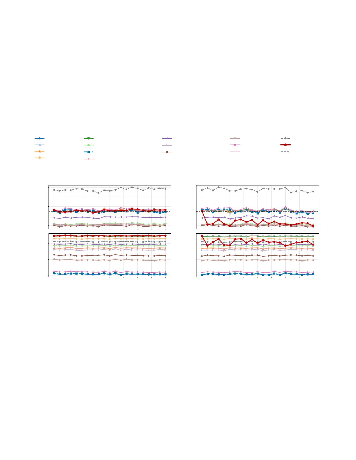
Err or -Contr olled Borr owing fr om External Data Using W asserstein Ambiguity Sets Y ui Kimura † ,1 and Shu T amano † ,2,3, ∗ † Equal contribution. 1 Nov artis Pharma K.K., 1-23-1 T oranomon, Minato-ku, T okyo 105-6333, Japan 2 Department of Multidisciplinary Sciences, Graduate School of Arts and Sciences, The Uni versity of T okyo, 3-8-1 K omaba, Meguro-ku, T okyo 153-8902, Japan 3 Department of Epidemiology , National Institute of Infectious Diseases, Japan Institute for Health Security , 1-23-1 T oyama, Shinjuku-ku, T okyo 162-0052, Japan ∗ Email: tamano-shu212@g.ecc.u-tokyo.ac.jp Abstract Incorporating external data can improv e the ef ﬁciency of clinical trials, b ut distributional mismatches between current and external populations threaten the v alidity of inference. While numerous dynamic borrowing methods exist, the calibration of their borrowing parameters relies mainly on ad hoc, simulation-based tuning. T o o vercome this, we propose BOND (Borro wing under Optimal Nonparametric Distributional rob ustness), a framew ork that formalizes data noncommensurability through W asserstein ambiguity sets centered at the current-trial distribution. By deriving sharp, closed-form bounds on the worst- case mean drift for both continuous and binary outcomes, we construct a distrib utionally robust, bias-corrected W ald statistic that ensures asymptotic type I error control uniformly ov er the ambiguity set. Importantly , BOND determines the optimal borro wing strength by maximizing a worst-case power proxy , con verting heuristic parameter tuning into a transparent, analytically tractable optimization problem. Furthermore, we demonstrate that many prominent borrowing methods can be reparameterized via an effecti ve borrowing weight, rendering our calibration frame work broadly applicable. Simulation studies and a real-world clinical trial application conﬁrm that BOND preserves the nominal size under unmeasured heterogeneity while achieving ef ﬁciency gains o ver standard borro wing methods. K eywords : Clinical trials; Distributionally robust optimization; Dynamic borrowing; Hybrid control; Information borro wing; W asserstein ball; 1 1 Intr oduction Randomized controlled trials remain the gold standard for e valuating treatment ef fects, principally be- cause randomization facilitates valid inference under minimal assumptions (International Conference on Harmonisation (ICH), 2000). Ho we ver , in many contemporary devel opment settings, recruiting a concurrently controlled arm of adequate size is practically challenging or ethically contentious. Con- straints such as small patient populations in rare diseases, slo w accrual rates, and the ethical dilemma of withholding ef fecti ve therapies ha ve fueled substantial interest in le veraging historical information or external comparators to augment current trials (Schmidli et al., 2020). Regulatory agencies hav e explicitly discussed the design and conduct of externally controlled trials (U.S. Food and Drug Administration, 2023; European Medicines Agenc y, 2025), and empirical surv eys document ho w external controls ha ve been used in regulatory submissions and decisions (Goring et al., 2019; Jahanshahi et al., 2021; Liu et al., 2025). Consequently , there is a pressing need for methodological frame works that improv e trial ef ﬁciency via borro wing while rigorously safeguarding operating characteristics. The fundamental challenge in borro wing from an external control arm is the potential noncommensura- bility (or lack of e xchangeability) between current and historical populations. Discrepancies in baseline characteristics, eligibility criteria, endpoint deﬁnitions, and secular trends in standard of care can introduce distributional shifts that induce bias and inﬂate type I error rates. Even modest drifts in the outcome distribution can shift the borro wing-based test statistic, leading to false rejections under the null h ypothesis (V iele et al., 2014; van Rosmalen et al., 2018). While causal inference techniques, such as propensity score weighting, can adjust for observed covariate imbalance, they cannot account for residual biases arising from unmeasured confounding or unobserved outcome drifts (Rippin et al., 2022). Therefore, a critical statistical problem is how to quantify and control for these distrib utional mismatches in a way that is transparent and satisﬁes regulatory rigor re garding error control. A v ast literature addresses adapti ve borro wing, broadly categorized into three streams. First, frequentist approaches employ test-then-pool (TTP) procedures or dynamic pooling strategies based on similarity tests (V iele et al., 2014; Li et al., 2020; Okada et al., 2024). Second, Bayesian dynamic borrowing methods introduce explicit parameters controlling the extent of borrowing, including po wer priors and their variants (Ibrahim and Chen, 2000; Ibrahim et al., 2003, 2015; Pawel et al., 2023), commensurate priors (Hobbs et al., 2011, 2012), and mixture-based constructions such as rob ust meta-analytic-predictiv e (MAP) priors and related e xchangeability models (Neuenschw ander et al., 2010; Schmidli et al., 2014; Neuenschwander et al., 2016; Kaizer et al., 2018; Y ang et al., 2023; Alt et al., 2024). Third, hybrid strategies combine borrowing with explicit cov ariate adjustment or selecti ve borrowing mechanisms, including propensity-score-integrated priors (Liu et al., 2021; Lu et al., 2022; W ang et al., 2022), case- weighted po wer priors (Kwiatko wski et al., 2024), and adapti ve hybrid control designs (Guo et al., 2024). Despite their dif ferences, these methods share a common reliance on tunable quantities such as discount 2 factors, precision parameters, and mixture weights that dictate the e xtent of borro wing. A persistent limitation in current practice is that the calibration of these borro wing parameters remains largely heuristic. T ypically , practitioners select discount factors based on extensi ve simulations under a speciﬁc set of designer -speciﬁed heterogeneity scenarios (P an et al., 2017; Psioda and Ibrahim, 2019; Eggleston et al., 2021; Ling et al., 2021; Khanal et al., 2025; Demartino et al., 2025). While this approach assesses performance under assumed conditions, it lacks explicit guarantees ag ainst de viations outside those scenarios. If strict type I error control is demanded against arbitrary incompatibility , the borrowing weight must tri vially collapse to zero (Psioda and Ibrahim, 2019; K opp-Schneider et al., 2020; Bennett et al., 2021; Lee, 2024; Gao et al., 2025). T o overcome this all-or -nothing tension, we require a framework that (i) explicitly deﬁnes a tolerance set of admissible heterogeneity and (ii) optimizes borro wing performance within that set. In this paper , we propose BOND (Borrowing under Optimal Nonparametric Distrib utional robustness), a frame work for integrati ng historical data under distributional uncertainty . Lev eraging tools from optimal transport (V illani, 2009) and distrib utionally rob ust optimization (DR O) (Mohajerin Esfahani and Kuhn, 2018; Blanchet and Murthy, 2019; Gao and Kleywegt, 2023; Kuhn et al., 2025), BOND formalizes noncommensurability by deﬁning the admissible discrepanc y as a W asserstein ball of radius ρ centered at the current-arm distrib ution. Under this geometric formulation, we parameterize borro wing strength via an ef fecti ve borro wing weight (EBW), which uniﬁes a broad class of estimators (see Appendix A for details), and deriv e tight, closed-form bounds on the worst-case mean drift for both continuous and binary outcomes. W e then construct a distributionally robust test that explicitly subtracts this worst-case bias, guaranteeing asymptotic type I error control uniformly o ver the ambiguity set. Finally , BOND identiﬁes the optimal borrowing strength by solving a minimax problem: maximizing a worst-case power proxy subject to the robust size constraint. Through simulations and a real-data application, we demonstrate ho w the radius ρ replaces ad hoc tuning by acting as a transparent, analytically tractable sensitivity parameter for regulatory decision-making. The remainder of the paper is organized as follows. Section 2 introduces the notation, the borrowing frame work, and the concept of W asserstein ambiguity sets. Section 3 details the proposed distrib utionally robust bias correction and the optimal weight calibration. Section 4 presents simulation results ev aluating operating characteristics. Section 5 applies the method to real-world clinical data. Section 6 concludes with a discussion of implications, limitations, and future directions. 3 2 Pr eliminaries 2.1 Pr oblem Setup Let ( X , B X ) be a measurable space for baseline covariates, and let Y denote the outcome space. W e consider tw o outcome types: (i) binary outcomes with Y = { 0 , 1 } , and (ii) continuous outcomes with Y = R , assuming E [ Y 2 ] < ∞ . Data are observ ed from two sources: a current randomized clinical trial ( j = C ) and a historical trial ( j = H ). For subject i in trial j , we observ e the tuple Z j,i : = ( A j,i , X j,i , Y j,i ) ∈ { 0 , 1 } × X × Y , where A j,i ∈ { 0 , 1 } denotes the treatment assignment ( 1 for experimental, 0 for control). For each arm a ∈ { 0 , 1 } and trial j ∈ { C , H } , let P a j denote the conditional probability measure of the co va riate- outcome pair ( X , Y ) : P a j : = L  ( X , Y )   A = a, j  , deﬁned on the product space Z : = X × Y equipped with B X ⊗ B Y . The marginal mean outcome in arm a of trial j is deﬁned as µ a j : = E P a j [ Y ] . For binary outcomes, this simpliﬁes to the response probability µ a j = P ( Y = 1 | A = a, j ) . The av erage treatment effect in the current trial on the mean-dif ference scale is θ C : = µ 1 C − µ 0 C . Similarly , the historical mean dif ference is θ H : = µ 1 H − µ 0 H . T o formalize between-trial heterogeneity without relying on speciﬁc parametric assumptions, we introduce a parameter γ ∈ Γ indexing a f amily of candidate historical laws { P a H ( γ ) } γ ∈ Γ . Let µ a H ( γ ) : = E P a H ( γ ) [ Y ] be the mean outcome under a speciﬁc heterogeneity le vel γ . The treatment effect in the historical population is denoted by θ H ( γ ) : = µ 1 H ( γ ) − µ 0 H ( γ ) . W e deﬁne the discrepancy function δ : Γ → R such that θ H ( γ ) = θ C + δ ( γ ) . This discrepancy can be decomposed into arm-speciﬁc mean shifts. Deﬁne the drift of the historical arm a relati ve to the current arm as ∆ a ( γ ) : = µ a H ( γ ) − µ a C , a ∈ { 0 , 1 } . It follo ws that δ ( γ ) = ∆ 1 ( γ ) − ∆ 0 ( γ ) . Throughout this paper , the pair (∆ 0 ( γ ) , ∆ 1 ( γ )) serves as the suf ﬁcient statistic for the bias induced by external information. 4 Remark 2.1 (Extensions beyond two arms and a single historical source) . For clarity of exposition, we focus on a binary treatment A ∈ { 0 , 1 } and a single historical source. Howe ver , the proposed framew ork extends naturally to (i) multi-arm trials with ﬁnitely many treatment lev els and (ii) borro wing from multiple historical datasets. These extensions are achiev ed by indexing arms and sources and replacing scalar borro wing weights with vectors. A formal generalization to the multi-arm/multi-source setting, including the robust bias correction and rob ust noncentrality parameter for arbitrary linear contrasts, is provided in Appendix B. 2.2 Effectiv e Borro wing Estimators Let n j be the total sample size of trial j , with realized arm sizes n j,a : = n j X i =1 1 { A j,i = a } , a ∈ { 0 , 1 } , j ∈ { C , H } . W e treat the sample sizes ( n j,a ) as ﬁxed or condition on them throughout. Deﬁne the arm-speciﬁc sample mean in trial j by ¯ Y j,a : = 1 n j,a X i : A j,i = a Y j,i , ( n j,a ≥ 1) . W e introduce a borrowing parameter λ = ( λ 0 , λ 1 ) ∈ Λ : = [0 , Λ 0 ] × [0 , Λ 1 ] , where Λ a represents a maximal borro wing cap (e.g., Λ a = 1 corresponds to the weight of the full historical sample). If only historical controls are av ailable, one may set n H, 1 = 0 and ﬁx λ 1 = 0 . The ef fecti ve borro wing estimator for the mean of arm a is deﬁned as: ˆ µ a ( λ a ) : =      n C,a ¯ Y C,a + λ a n H,a ¯ Y H,a n C,a + λ a n H,a , n H,a ≥ 1 , ¯ Y C,a , n H,a = 0 . (1) This formulation encompasses a wide range of Bayesian borro wing methods (see Appendix A for the details). W e deﬁne the EBW as: w a ( λ a ) : = λ a n H,a n C,a + λ a n H,a ∈ [0 , 1) , which yields the con vex combination ˆ µ a ( λ a ) = (1 − w a ( λ a )) ¯ Y C,a + w a ( λ a ) ¯ Y H,a . The resulting estimator for the treatment ef fect is ˆ θ ( λ ) : = ˆ µ 1 ( λ 1 ) − ˆ µ 0 ( λ 0 ) . Its expectation satisﬁes: E  ˆ θ ( λ )  = θ C + w 1 ( λ 1 )∆ 1 ( γ ) − w 0 ( λ 0 )∆ 0 ( γ ) . (2) (2) highlights that if the historical data are not perfectly commensurate (i.e., ∆ a  = 0 ), the borrowing induces a bias of w 1 ∆ 1 ( γ ) − w 0 ∆ 0 ( γ ) . W ithout correction, this shift can inﬂate the type I error rate. 5 2.3 W asserstein Ambiguity Sets T o quantify distributional differences between current and historical arms without committing to a parametric model, we employ W asserstein ambiguity sets (V illani, 2009; Mohajerin Esfahani and K uhn, 2018; Blanchet and Murthy, 2019; Gao and Kle ywegt, 2023). Let ( X , d X ) be a metric space for co variates, and equip Y with the Euclidean distance. On the product space Z = X × Y , we deﬁne the ground metric: d  ( x, y ) , ( x ′ , y ′ )  : = d X ( x, x ′ ) + | y − y ′ | . (3) Remark 2.2 . The additive structure of the metric in (3) is deliberate. First, it ensures that the outcome mapping ( x, y ) 7→ y is 1 -Lipschitz, which is essential for deriving sharp bounds on the mean shift. Second, it interprets the cost of transport as a sum of cov ariate mismatch and outcome drift. While other metrics (e.g., L p -combinations) are possible, the additi ve form of fers a clear interpretation where a unit shift in outcome Y contrib utes directly to the transport cost. Let P 1 ( Z ) denote the set of Borel probability measures on Z with ﬁnite ﬁrst moment with respect to d . The 1 -W asserstein distance between two measures P , Q ∈ P 1 ( Z ) is deﬁned as: W 1 ( P , Q ) : = inf π ∈ Π( P,Q ) Z Z ×Z d ( z , z ′ ) π (d z , d z ′ ) , where Π( P , Q ) denotes the set of couplings with mar ginals P and Q . For a speciﬁed radius ρ a ≥ 0 , we deﬁne the arm-speciﬁc W asserstein ambiguity set (or ball) centered at P a C by U a ( ρ a ) : =  Q ∈ P 1 ( Z ) : W 1 ( Q, P a C ) ≤ ρ a  . (4) The condition P a H ∈ U a ( ρ a ) formalizes the assumption that the historical distribution drifts from the current distribution by at most ρ a in terms of the W asserstein distance. W ithin this set, we identify the worst-case mean shifts: ∆ + a ( ρ a ) : = sup Q ∈U a ( ρ a )  E Q [ Y ] − µ a C  , ∆ − a ( ρ a ) : = inf Q ∈U a ( ρ a )  E Q [ Y ] − µ a C  . These bounds, ∆ + a and ∆ − a , represent the maximal positiv e and negati ve bias feasible under the constraint that the historical data are ρ a -compatible with the current trial. 3 Pr oposed Method W e refer to the proposed distributionally rob ust calibration-and-testing procedure as BOND. 3.1 W orst-Case Mean Shifts over W asserstein Balls The core of our proposal is to robustify the borrowing estimator against distributional shifts. The ﬁrst analytical step is to determine the worst-case expectation of the outcome Y within the W asserstein ambiguity set U a ( ρ a ) . Although this is generally an inﬁnite-dimensional optimization problem, the speciﬁc 6 structure of W 1 -transport cost with the ground metric (3) allo ws us to deri ve sharp, closed-form bounds (Mohajerin Esfahani and K uhn, 2018; Blanchet and Murthy, 2019; Kuhn et al., 2025). Proposition 3.1 (Closed-form worst-case mean shifts) . F ix an arm a ∈ { 0 , 1 } and let U a ( ρ a ) be deﬁned by (4) under the metric (3) . Assume P a C ∈ P 1 ( Z ) . (i) (Continuous outcome) If Y = R , then ∆ + a ( ρ a ) = ρ a , ∆ − a ( ρ a ) = − ρ a . (ii) (Binary outcome) If Y = { 0 , 1 } , then sup Q ∈U a ( ρ a ) E Q [ Y ] = min { µ a C + ρ a , 1 } , inf Q ∈U a ( ρ a ) E Q [ Y ] = max { µ a C − ρ a , 0 } , equivalently , ∆ + a ( ρ a ) = min { ρ a , 1 − µ a C } , ∆ − a ( ρ a ) = − min { ρ a , µ a C } . See Appendix D.2 for the proof. Proposition 3.1 turns an inﬁnite-dimensional DR O problem over a W asserstein ball into an explicit, closed-form bound on the arm-wise mean drift. As a result, the rob ust bias correction can be computed by simple arithmetic (no optimization solver is needed), which enables fast calibration of the borro wing parameters and transparent sensitivity interpretation of the radius ρ a . 3.2 Rob ust Bias Correction and T est Deﬁnition W e consider the one-sided hypothesis H 0 : θ C ≤ 0 vs. H 1 : θ C > 0 . Let z 1 − α denote the (1 − α ) quantile of the standard normal distrib ution. For each λ ∈ Λ , the worst-case bias in the rejection direction is: b + ( λ ) : = sup Q 1 ∈U 1 ( ρ 1 ) Q 0 ∈U 0 ( ρ 0 ) h w 1 ( λ 1 )  E Q 1 [ Y ] − µ 1 C  − w 0 ( λ 0 )  E Q 0 [ Y ] − µ 0 C  i . (5) Proposition 3.2 (Closed-form of b + ( λ ) ) . F or any λ ∈ Λ with w a ( λ a ) ≥ 0 , b + ( λ ) = w 1 ( λ 1 )∆ + 1 ( ρ 1 ) − w 0 ( λ 0 )∆ − 0 ( ρ 0 ) . In particular , under Pr oposition 3.1, b + ( λ ) =    w 1 ( λ 1 ) ρ 1 + w 0 ( λ 0 ) ρ 0 , Y = R , w 1 ( λ 1 ) min { ρ 1 , 1 − µ 1 C } + w 0 ( λ 0 ) min { ρ 0 , µ 0 C } , Y = { 0 , 1 } . See Appendix D.3 for the proof. Proposition 3.2 shows that the worst-case bias in the rejection direction decomposes arm-by-arm and depends on λ only through the EBW w a ( λ a ) . Combined with Proposition 3.1, 7 this yields an explicit b + ( λ ) , making the robust test and subsequent λ -calibration computationally tri vial to e v aluate ov er Λ . W e deﬁne the asymptotic variance of ˆ θ ( λ ) as: s 2 ( λ ) : = V ar  ˆ θ ( λ )  = X a ∈{ 0 , 1 } "  1 − w a ( λ a )  2 σ 2 C,a n C,a + w a ( λ a ) 2 σ 2 H,a n H,a # , (6) where σ 2 j,a : = V ar( Y | A = a, j ) and the con vention is that the term w a ( λ a ) 2 σ 2 H,a /n H,a is set to 0 if n H,a = 0 . In practice, we estimate (6) via the pooled plug-in estimator . For ( j, a ) with n j,a ≥ 2 , let ˆ σ 2 j,a : = 1 n j,a − 1 X i : A j,i = a  Y j,i − ¯ Y j,a  2 , and deﬁne ˆ s 2 ( λ ) : = X a ∈{ 0 , 1 } "  1 − w a ( λ a )  2 ˆ σ 2 C,a n C,a + w a ( λ a ) 2 ˆ σ 2 H,a n H,a # , ˆ s ( λ ) : = p ˆ s 2 ( λ ) . (7) For binary outcomes, b + ( λ ) depends on the unkno wn µ a C . A natural implementation replaces µ a C by ¯ Y C,a in Proposition 3.2; denote the resulting plug-in bias by ˆ b + ( λ ) . For continuous outcomes, b + ( λ ) depends only on ( ρ 0 , ρ 1 ) and ( w 0 , w 1 ) . W e propose the distributionally rob ust W ald test φ λ : = 1 ( ˆ θ ( λ ) − ˜ b + ( λ ) ˆ s ( λ ) ≥ z 1 − α ) , (8) where ˜ b + ( λ ) = b + ( λ ) if b + ( λ ) is treated as kno wn theoretical benchmark and ˜ b + ( λ ) = ˆ b + ( λ ) for the practical plug-in version. Remark 3.3 (T wo-sided e xtension) . The main text focuses on the one-sided hypothesis H 0 : θ C ≤ 0 . A two-sided test for H ± 0 : θ C = 0 , H ± 1 : θ C  = 0 is obtained by introducing the worst-case bias in the ne gati ve rejection direction, b − ( λ ) : = inf Q 1 ∈U 1 ( ρ 1 ) Q 0 ∈U 0 ( ρ 0 ) h w 1 ( λ 1 ) { E Q 1 [ Y ] − µ 1 C } − w 0 ( λ 0 ) { E Q 0 [ Y ] − µ 0 C } i , and rejecting when either tail is signiﬁcant: φ ± λ : = 1 ( ˆ θ ( λ ) − ˜ b + ( λ ) ˆ s ( λ ) ≥ z 1 − α/ 2 or ˆ θ ( λ ) − ˜ b − ( λ ) ˆ s ( λ ) ≤ − z 1 − α/ 2 ) . Here ˜ b − ( λ ) is the benchmark b − ( λ ) or its plug-in version for binary outcomes. The closed-form of b − ( λ ) and the full proofs of distributionally rob ust size control are giv en in Appendix C. 8 3.3 Asymptotic Guarantees and Optimal Calibration W e introduce a minimal asymptotic framew ork. Assumption 3.4 (Sampling and moments) . For each ( j, a ) with n j,a ≥ 1 , the outcomes { Y j,i : A j,i = a } are i.i.d. with mean µ a j and v ariance σ 2 j,a < ∞ . Moreov er , the collections from dif ferent ( j, a ) are mutually independent. Assumption 3.5 (Asymptotic regime and nondegeneracy) . For each arm a , n C,a → ∞ and either n H,a → ∞ or n H,a = 0 . Additionally , σ 2 C,a > 0 for a ∈ { 0 , 1 } . Proposition 3.6 (Asymptotic normality) . Under Assumptions 3.4 and 3.5, for any ﬁxed λ ∈ Λ , ˆ θ ( λ ) −  θ C + w 1 ( λ 1 )∆ 1 − w 0 ( λ 0 )∆ 0  s ( λ ) − → d N (0 , 1) , wher e s ( λ ) is deﬁned in (6) . See Appendix D.4 for the proof. Proposition 3.6 provides a Gaussian approximation for the borro wing estimator ˆ θ ( λ ) with an explicit centering term that isolates the external-data bias component. This normal limit justiﬁes the W ald-type construction in (8) and is the k ey step that allo ws us to deri ve analytic size and po wer characterizations for each ﬁxed λ . W e now state the rob ust size guarantee, deﬁned with respect to the W asserstein ambiguity sets. Theorem 3.7 (Asymptotic distributionally robust size control) . F ix λ ∈ Λ . F or any ﬁxed ( θ C , P 0 H , P 1 H ) with θ C ≤ 0 and P a H ∈ U a ( ρ a ) , a ∈ { 0 , 1 } , under Assumptions 3.4 and 3.5, lim sup min a n C,a →∞ P ( φ λ = 1) ≤ α, wher e the pr obability is taken under the joint law induced by the i.i.d. sampling fr om ( P 0 C , P 1 C , P 0 H , P 1 H ) . See Appendix D.5 for the proof. Theorem 3.7 guarantees asymptotic type I error control uniformly over all historical-arm distributions lying in the W asserstein ambiguity sets. Thus, for any prespeciﬁed borro wing rule λ , the proposed bias correction provides a principled safeguard against false positi ves induced by lack of commensurability between current and external data. Proposition 3.8 (T ightness and minimality of the rob ust correction) . F ix λ ∈ Λ and consider the one-sided W ald-type test family φ λ,c : = 1 ( ˆ θ ( λ ) − c ˆ s ( λ ) ≥ z 1 − α ) , c ∈ R . (i) (Minimality) If c < b + ( λ ) , there e xists a null conﬁguration ( θ C , P 0 H , P 1 H ) with θ C = 0 and P a H ∈ U a ( ρ a ) lim inf min a n C,a →∞ P ( φ λ,c = 1) > α. Consequently , b + ( λ ) is the minimal constant corr ection r equir ed to guarantee distributionally r obust size contr ol over the joint ambiguity set U 0 ( ρ 0 ) × U 1 ( ρ 1 ) . 9 (ii) (T ightness) F or c = b + ( λ ) , the bound in Theor em 3.7 is tight in the minimax sense: sup θ C ≤ 0 ,P a H ∈U a ( ρ a ) lim min a n C,a →∞ P ( φ λ = 1) = α . See Appendix D.6 for the proof. Proposition 3.8 shows that the proposed rob ust correction b + ( λ ) is not only suf ﬁcient but also necessary (within the class of constant-shift W ald tests) for distrib utionally robust size control ov er U 0 ( ρ 0 ) × U 1 ( ρ 1 ) . In particular , an y smaller correction c < b + ( λ ) leads to asymptotic type I error inﬂation under some admissible historical drift, while the choice c = b + ( λ ) attains the nominal le vel α under an explicit least-f a vorable conﬁguration, implying that Theorem 3.7 is minimax-sharp and cannot be further tightened without strengthening assumptions or enlarging the test class. T o characterize power , ﬁx a target alternati ve ef fect θ 1 > 0 and deﬁne the robust po wer P o w rob ( λ ; θ 1 ) : = inf P 1 H ∈U 1 ( ρ 1 ) ,P 0 H ∈U 0 ( ρ 0 ) P θ C = θ 1  φ λ = 1  . Theorem 3.9 (Asymptotic rob ust po wer and the rob ust noncentrality parameter) . F ix θ 1 > 0 and λ ∈ Λ . Under Assumptions 3.4 and 3.5, lim min a n C,a →∞ P o w rob ( λ ; θ 1 ) = 1 − Φ  z 1 − α − κ ( λ )  , wher e Φ is the standar d normal cumulative distribution function and κ ( λ ) : = θ 1 − w 1 ( λ 1 )  ∆ + 1 ( ρ 1 ) − ∆ − 1 ( ρ 1 )  − w 0 ( λ 0 )  ∆ + 0 ( ρ 0 ) − ∆ − 0 ( ρ 0 )  s ( λ ) . (9) See Appendix D.7 for the proof. Theorem 3.9 yields an explicit asymptotic lower bound on power in terms of the robust noncentrality parameter κ ( λ ) . This conv erts the choice of the borrowing parameter from ad-hoc scenario-based simulation to a direct, analytically tractable optimization problem: maximize κ ( λ ) (equi v alently rob ust power) while preserving w orst-case size control. The test (8) controls worst-case type I error asymptotically for each ﬁx ed λ . Therefore, it is natural to select λ by maximizing the rob ust po wer lo wer bound. Corollary 3.10 (Rob ust-po wer optimal borro wing weight exists) . Assume Λ = [0 , Λ 0 ] × [0 , Λ 1 ] is compact. Under Assumptions 3.4 and 3.5, the map λ 7→ κ ( λ ) in (9) is continuous on Λ . Hence, ther e exists at least one maximizer λ ∗ ∈ arg max λ ∈ Λ P o w rob ( λ ; θ 1 ) = arg max λ ∈ Λ κ ( λ ) . See Appendix D.8 for the proof. Corollary 3.10 ensures that the proposed DR O-based calibration problem is well-posed: an optimal borrowing parameter λ ∗ exists on the prespeciﬁed feasible set Λ . This guarantees that the method produces a concrete, implementable recommendation rather than only a conceptual criterion. Remark 3.11 . The optimization in Corollary 3.10 formalizes DR O-based calibration of the borro wing degree: we maximize a worst-case (ov er W asserstein ambiguity sets) power functional while maintaining 10 worst-case type I error control (Theorem 3.7). This contrasts with common ad-hoc calibrations of discounting parameters by simulation for speciﬁc scenarios, as in many implementations of power priors, commensurate priors, and MAP/robust MAP priors. 3.4 Implementation and Algorithm This subsection summarizes the fully implementable BOND procedure, which calibrates the borro wing parameter λ by maximizing a plug-in version of the robust noncentrality parameter , follo wed by the robust W ald test at the selected ˆ λ . Importantly , the procedure requires only arm-le vel summary statistics ( n j,a , ¯ Y j,a , ˆ σ 2 j,a ) , making it directly applicable to aggregate historical data. 3.4.1 Plug-In Robust P ower Criterion Recall the robust noncentrality parameter κ ( λ ) in (9) . Let D a ( ρ a ) : = ∆ + a ( ρ a ) − ∆ − a ( ρ a ) denote the arm-wise worst-case mean-drift range. By Proposition 3.1, this simpliﬁes to D a ( ρ a ) =    2 ρ a , Y = R , min { ρ a , 1 − µ a C } + min { ρ a , µ a C } , Y = { 0 , 1 } . For the latter , we use the plug-in estimator ˆ D a ( ρ a ) obtained by replacing µ a C with ¯ Y C,a . W e deﬁne the plug-in robust noncentrality parameter as ˆ κ ( λ ) : = θ 1 − w 1 ( λ 1 ) ˆ D 1 ( ρ 1 ) − w 0 ( λ 0 ) ˆ D 0 ( ρ 0 ) ˆ s ( λ ) , (10) where ˆ s ( λ ) is gi ven in (7) . The corresponding rob ust po wer proxy , d P o w rob ( λ ; θ 1 ) : = 1 − Φ( z 1 − α − ˆ κ ( λ )) , is strictly monotone in ˆ κ ( λ ) . Because Λ is compact and ˆ κ ( λ ) is continuous whenev er ˆ s ( λ ) > 0 , the maximizer set is non-empty . T o ensure a single-valued selection, we adopt a deterministic tie-breaking rule Sel( · ) that selects the maximizer with the smallest Euclidean norm, breaking remaining ties lexicographically . The data-driv en borro wing parameter is then: ˆ λ : = Sel  arg max λ ∈ Λ ˆ κ ( λ )  . (11) If only historical controls are a v ailable ( n H, 1 = 0 ), we ﬁx λ 1 = 0 and optimize ov er λ 0 ∈ [0 , Λ 0 ] . Algorithm 1 details the complete end-to-end procedure. 3.4.2 Asymptotic V alidity of Data-Driven Calibration While Theorem 3.7 establishes size control for a ﬁxed λ , Algorithm 1 selects ˆ λ adapti vely . W e now formally justify that this data-dri ven test φ ˆ λ retains asymptotic type I error control. 11 Algorithm 1 BOND: Borro wing under Optimal Nonparametric Distributional rob ustness Require: Signiﬁcance le vel α ∈ (0 , 1) ; target alternati ve ef fect θ 1 > 0 ; radii ( ρ 0 , ρ 1 ) ; feasible set Λ = [0 , Λ 0 ] × [0 , Λ 1 ] ; arm-le vel summaries { ( n j,a , ¯ Y j,a , ˆ σ 2 j,a ) } j ∈{ C ,H } ,a ∈{ 0 , 1 } (con vention: n H,a = 0 if unav ailable). Ensure: Selected parameter ˆ λ , test statistic T ( ˆ λ ) , and decision φ ˆ λ ∈ { 0 , 1 } . 1: Compute EBWs w a ( λ a ) = λ a n H,a / ( n C,a + λ a n H,a ) for a ∈ { 0 , 1 } (set w a ( λ a ) = 0 if n H,a = 0 ). 2: F or each λ ∈ Λ , compute ˆ µ a ( λ a ) via (1), ˆ θ ( λ ) = ˆ µ 1 ( λ 1 ) − ˆ µ 0 ( λ 0 ) , and ˆ s ( λ ) via (7). 3: F or each λ ∈ Λ , compute the bias correction ˜ b + ( λ ) : ˜ b + ( λ ) =    w 1 ( λ 1 ) ρ 1 + w 0 ( λ 0 ) ρ 0 , Y = R , w 1 ( λ 1 ) min { ρ 1 , 1 − ¯ Y C, 1 } + w 0 ( λ 0 ) min { ρ 0 , ¯ Y C, 0 } , Y = { 0 , 1 } . 4: Compute ˆ κ ( λ ) via (10) and select ˆ λ via (11). 5: Compute the rob ust W ald statistic and output the decision: T ( ˆ λ ) : = ˆ θ ( ˆ λ ) − ˜ b + ( ˆ λ ) ˆ s ( ˆ λ ) , φ ˆ λ : = 1 { T ( ˆ λ ) ≥ z 1 − α } . Let a n : = √ n C + n H → ∞ . Maximizing ˆ κ ( λ ) is equi valent to maximizing the rescaled objecti ve ˆ ¯ κ ( λ ) : = a − 1 n ˆ κ ( λ ) . Let ¯ κ ( λ ) denote its population counterpart, and deﬁne the theoretical optimal parameter λ ∗ : = Sel(arg max λ ∈ Λ ¯ κ ( λ )) . Assumption 3.12 (W ell-separated maximizer) . The population optimizer λ ∗ is well-separated: for ev ery ε > 0 , there exists δ ε > 0 such that for all sufﬁciently lar ge n , sup ∥ λ − λ ∗ ∥ 2 ≥ ε ¯ κ ( λ ) ≤ ¯ κ ( λ ∗ ) − δ ε . Proposition 3.13 (Rob ust size control with adaptiv e ˆ λ ) . Suppose Assumptions 3.4 – 3.5 and 3.12 hold. Let ˆ λ be selected via (11) . Then, for any null conﬁguration ( θ C , P 0 H , P 1 H ) with θ C ≤ 0 and P a H ∈ U a ( ρ a ) , the adaptive test φ ˆ λ : = 1 { ( ˆ θ ( ˆ λ ) − b + ( ˆ λ )) / ˆ s ( ˆ λ ) ≥ z 1 − α } satisﬁes: lim sup min a n C,a →∞ P  φ ˆ λ = 1  ≤ α. See Appendix D.9 for the proof. Proposition 3.13 formally justiﬁes the data-driv en calibration step, guaranteeing that practitioners can adapti vely optimize borro wing weights to maximize po wer without inﬂating the worst-case type I error . Remark 3.14 (Safe guards for adapti ve implementation) . Assumption 3.12 generically holds when ¯ κ ( λ ) has a unique maximizer . If one wishes to a void relying on uniqueness, a deterministic v anishing regularizer (e.g., subtracting η n ∥ λ ∥ 2 2 where η n → ∞ but η n /a n → 0 ) can enforce stability without asymptotically altering the objecti ve. Furthermore, for binary outcomes, Proposition 3.13 utilizes the oracle correction b + ( λ ) dependent on true µ a C . A conservati ve, fully data-dri ven implementation can rely on the uni versal bounds ∆ + a ( ρ a ) ≤ ρ a and ∆ − a ( ρ a ) ≥ − ρ a , yielding b univ + ( λ ) : = w 1 ( λ 1 ) ρ 1 + w 0 ( λ 0 ) ρ 0 ≥ b + ( λ ) . Alterna- 12 ti vely , the plug-in correction in Algorithm 1 is exact with probability tending to one under the interior condition ρ a < min { µ a C , 1 − µ a C } . 4 Numerical Experiments 4.1 Experimental Setup W e conducted extensi ve numerical e xperiments to ev aluate the ﬁnite-sample operating characteristics of BOND against a suite of standard borrowing rules. W e simulated a current randomized trial ( n C = 200 ) and a historical dataset ( n H = 500 ) with baseline co v ariates X ∈ R 2 for both continuous and binary outcomes. T o assess robustness against between-trial noncommensurability , we v aried a scalar heterogeneity index γ ranging from 0 to 2 in increments of 0 . 1 . W e considered three data-generating cases representing common mechanisms of incompatibility: (i) Commensurate (no cov ariate shift, no drift; historical data include both arms), (ii) Cov ariate shift + effect modiﬁcation (shifted historical covariates with treatment-co v ariate interaction inducing γ -dependent marginal ef fect differences), and (iii) Control drift (historical control-only) (historical controls only with a control-arm mean drift of magnitude γ ). W e compared BOND against representativ e frequentist and Bayesian borrowing paradigms implemented in the accompanying code, including Current-only (no borro wing), Naiv e pooling (full borro wing), ﬁxed- weight EBW rules, the power prior (Ibrahim and Chen, 2000), the commensurate prior (Hobbs et al., 2012), and robust MAP priors (Schmidli et al., 2014). For all methods, we tested the one-sided hypothesis H 0 : θ C ≤ 0 at lev el α = 0 . 025 using standardized W ald-type statistics. For BOND, we e v aluated tw o radius speciﬁcations: an oracle radius (true ρ a = | µ a H − µ a C | ) and a data-dri ven proxy ˆ ρ a = c c W 1 ( b P a C , b P a H ) with an inﬂation multiplier c = 1 . 5 . Complete details of the data-generating mechanisms, hyperparameter settings, and comprehensiv e operating characteristic curves for all methods, including TTP and other borro wing methods, are provided in Appendix E. 4.2 Results 4.2.1 Adaptive Borr owing Behavior The proposed DR O calibration transparently modulates borrowing based on the speciﬁed tolerance for discrepancy . Figure 1 visualizes the borro wing le vels selected by BOND under the data-dri ven radii for continuous outcomes. When true noncommensurability is introduced (under the Co v ariate shift + ef fect modiﬁcation and Control drift scenarios), BOND exhibits a sharp, adaptiv e switching behavior: it permits near-full borro wing at γ = 0 , b ut rapidly attenuates the historical weight to zero as γ increases beyond 0 . 1 , successfully guarding against bias. 13 λ ∗ 0 λ ∗ 1 w 0 ( λ ∗ ) w 1 ( λ ∗ ) 0 . 00 0 . 25 0 . 50 0 . 75 1 . 00 1 . 25 1 . 50 1 . 75 2 . 00 γ 0 . 0 0 . 2 0 . 4 0 . 6 0 . 8 1 . 0 Borrowing level 0 . 00 0 . 25 0 . 50 0 . 75 1 . 00 1 . 25 1 . 50 1 . 75 2 . 00 γ 0 . 0 0 . 2 0 . 4 0 . 6 0 . 8 1 . 0 Borrowing level Figure 1: BOND-calibrated borrowing le vels v ersus γ for continuous outcomes under data-dri ven radii ( c = 1 . 5 ). Each panel plots the calibrated discount factors ( λ ∗ 0 , λ ∗ 1 ) and the implied EBW ( w 0 ( λ ∗ 0 ) , w 1 ( λ ∗ 1 )) . Left: cov ariate shift + effect modiﬁcation. Right: control drift with historical controls only (so λ ∗ 1 ≡ 0 ). 4.2.2 T ype I Error and Po wer T rade-offs T able 1 summarizes the worst-case operating characteristics o ver the γ grid for continuous outcomes, and Figure 2 illustrates these continuous dynamics across the full range of heterogeneity . Aggressiv e strate gies (e.g., Nai ve pooling, ﬁxed λ = 0 . 5 , or standard po wer priors) achiev e high po wer under the Commensurate scenario b ut suf fer catastrophic type I error inﬂation ( ≈ 1 . 000 ) as heterogeneity gro ws under the Cov ariate shift + effect modiﬁcation scenario, rendering them unacceptable for regulatory purposes. In contrast, Figure 2 (left panels) demonstrates that BOND, robust MAP , and the commensurate prior successfully maintain strict type I error control e ven as γ increases. Importantly , BOND achie ves this rob ustness without sacriﬁcing utility . In the Commensurate scenario, BOND boosts the w orst-case po wer to 0 . 773 , nearly doubling the ef ﬁciency of the Current-only design ( 0 . 402 ). Furthermore, under the Control drift scenario (Figure 2, right panels), sev eral dynamic priors become some what conservati ve and suf fer a sev ere power collapse due to borrowing historical controls in the wrong direction. Howe ver , BOND consistently controls the type I error near the nominal le vel while preserving substantially higher power than these competing robust methods, re verting to the Current-only baseline po wer ( 0 . 400 ) by adapti vely setting λ ∗ 0 ≈ 0 . Exhausti ve graphical proﬁles and tables for all scenarios, methods, endpoints, and radius speciﬁcations (including oracle radii) are provided in Appendix E.2. 14 T able 1: W orst-case operating characteristics ov er γ ranging from 0 to 2 in increments of 0 . 1 for continuous outcomes under data-driv en radii ( c = 1 . 5 ). W e report the maximum empirical type I error and the minimum empirical po wer for a focused subset of methods. Commensurate Cov ariate shift + Mod. Control drift (historical control-only) Method max γ \ T yp eI min γ \ P ow er max γ \ T yp eI min γ \ P ow er max γ \ T yp eI min γ \ P ow er Current-only 0 . 029 0 . 402 0 . 027 0 . 326 0 . 028 0 . 400 Naiv e pooling 0 . 028 0 . 892 1 . 000 0 . 826 0 . 026 0 . 000 Fixed λ = 0 . 5 0 . 028 0 . 854 1 . 000 0 . 777 0 . 026 0 . 000 Power prior ( λ = 0 . 5 ) 0 . 013 0 . 765 0 . 984 0 . 669 0 . 022 0 . 000 Commensurate prior ( τ = 1 ) 0 . 028 0 . 406 0 . 042 0 . 352 0 . 027 0 . 348 Robust MAP ( ϵ = 0 . 2 ) 0 . 012 0 . 736 0 . 081 0 . 144 0 . 028 0 . 026 BOND (data-driv en) 0 . 025 0 . 773 0 . 027 0 . 326 0 . 028 0 . 400 Current-only Naive p o oling Fixed λ =0.50 Po wer prior( λ =0.50) Commensurate prior( τ =1.00) Robust MAP(  =0.20) BOND α 0 . 00 0 . 25 0 . 50 0 . 75 1 . 00 Type-I error 0 . 00 0 . 25 0 . 50 0 . 75 1 . 00 1 . 25 1 . 50 1 . 75 2 . 00 γ 0 . 2 0 . 4 0 . 6 0 . 8 1 . 0 Po wer 0 . 00 0 . 01 0 . 02 Type-I error 0 . 00 0 . 25 0 . 50 0 . 75 1 . 00 1 . 25 1 . 50 1 . 75 2 . 00 γ 0 . 0 0 . 2 0 . 4 0 . 6 Po wer Figure 2: Empirical type I error (top) and power (bottom) versus γ for continuous outcomes under data-dri ven radii ( c = 1 . 5 ). Left: cov ariate shift + effect modiﬁcation. Right: control drift with historical controls only (so λ ∗ 1 ≡ 0 ). 5 Real-W orld Data Experiments 5.1 Real-W orld Dataset W e illustrate the proposed method using aggregate data from two randomized studies in previously treated metastatic colorectal cancer (mCRC). The goal is to e v aluate the treatment ef fect of panitumumab plus FOLFIRI versus FOLFIRI alone on the binary objecti ve response rate (ORR), utilizing the panitumumab 15 T able 2: Real-world ORR analysis (representativ e methods). W e report the estimated control response ˆ µ 0 , estimated treatment ef fect ˆ θ = ˆ µ 1 − ˆ µ 0 , the 95% interv al width relati ve to Current-only , the effecti v e borro wed historical control sample size n eﬀ hist , and the one-sided p -v alue for H 0 : θ C ≤ 0 . Method ˆ µ 0 ˆ θ W idth ratio n eﬀ hist p Current-only 0 . 128 0 . 156 1 . 000 0 7 . 7 × 10 − 10 Nai ve pooling 0 . 263 0 . 022 0 . 946 610 0 . 186 Fixed λ = 0 . 5 0 . 220 0 . 063 0 . 930 305 0 . 005 Po wer prior ( λ = 0 . 5 ) 0 . 220 0 . 062 0 . 989 305 0 . 008 Commensurate prior ( τ = 1 ) 0 . 132 0 . 152 1 . 004 4 2 . 2 × 10 − 9 Robust MAP ( ϵ = 0 . 2 ) 0 . 130 0 . 155 1 . 001 0 7 . 8 × 10 − 10 BOND ( ρ 0 = 0 ) 0 . 220 0 . 065 0 . 930 294 0 . 004 trial (Peeters et al., 2010) as the current study ( j = C ). W e borrow external control information from the placebo plus FOLFIRI arm of the VELOUR study (T abernero et al., 2014) ( j = H ). Because the experimental regimens dif fer , we calibrate borro wing exclusi vely for the control arm ( λ 1 = 0 , λ 0 ∈ [0 , Λ 0 ] ). This dataset presents a se vere stress test for dynamic borro wing: the observ ed ORR in the historical control is 0 . 367 , markedly higher than the 0 . 128 observed in the current control. This absolute gap of 0 . 239 implies substantial noncommensurability (e.g., secular trends or unmeasured prognostic dif ferences). 5.2 Results and Interpr etation T able 2 compares BOND (at ρ 0 = 0 ) against standard baselines. The Current-only analysis demonstrates a highly signiﬁcant treatment ef fect ( ˆ θ = 0 . 156 , p < 0 . 001 ). Howe ver , Naiv e pooling forcefully incorporates the highly discordant historical controls, artiﬁcially inﬂating the estimated control ORR to 0 . 263 . This sev erely attenuates the estimated treatment effect to ˆ θ = 0 . 022 , completely destroying statistical signiﬁcance ( p = 0 . 186 ) despite yielding a narro wer conﬁdence interval. Fixed-weight priors ( λ = 0 . 5 ) similarly dilute the effect. Con versely , adapti ve rob ust priors (Commensurate, Robust MAP) detect the massiv e conﬂict, effecti vely shutting of f borrowing ( n eﬀ hist ≈ 0 ) and recov ering the Current-only result, but f ailing to provide an y efﬁciency g ain. Unlike these all-or -nothing adapti ve methods, BOND e v aluated at ρ 0 = 0 proacti vely optimizes for maximum po wer by borro wing aggressiv ely ( n eﬀ hist = 294 ). As sho wn in T able 2, although this inevitably attenuates the point estimate ( ˆ θ = 0 . 065 ), BOND uniquely secures the narrowest conﬁdence interv al (width ratio 0 . 930 ) while successfully preserving statistical signiﬁcance ( p = 0 . 004 ), thus demonstrating an optimal balance between ef ﬁciency and v alidity . Figure 3 illustrates the unique v alue of the BOND frame work via sensitivity analysis o ver ρ 0 . At ρ 0 = 0 , BOND optimizes for maximum po wer , borrowing aggressively ( n eﬀ hist = 294 ) and yielding a tight, but 16 Current-only Naive p o oling Fixed λ =0.50 Po wer prior( λ =0.50) Commensurate prior( τ =1.00) Robust MAP(  =0.20) BOND 0 . 000 0 . 025 0 . 050 0 . 075 0 . 100 0 . 125 0 . 150 0 . 175 0 . 200 ρ 0 . 00 0 . 05 0 . 10 0 . 15 0 . 20 ˆ θ with 95% CI 0 . 000 0 . 025 0 . 050 0 . 075 0 . 100 0 . 125 0 . 150 0 . 175 0 . 200 ρ 0 100 200 300 400 500 600 Borrow ed historical n (arm 0) Figure 3: Real-world sensitivity to ρ 0 for BOND vs. baselines. Left: Estimated treatment ef fect ˆ θ with 95% robust conﬁdence interv als (CIs) versus the tolerance radius ρ 0 . Right: Effecti ve borro wed historical control sample size ( n eﬀ hist ) versus ρ 0 . attenuated, estimate ( ˆ θ = 0 . 065 ). As the tolerance for unmeasured drift increases (e.g., ρ 0 → 0 . 05 ), BOND mathematically acknowledges the inﬂated w orst-case bias and automatically attenuates the borro wing weight to protect the type I error ( n eﬀ hist drops to 12 ). The effect estimate correspondingly climbs back to 0 . 150 . F or ρ 0 ≥ 0 . 10 , BOND recognizes that the potential bias ov erwhelms any variance reduction, setting λ ∗ 0 = 0 and perfectly re verting to the Current-only analysis. This analysis demonstrates that BOND provides a principled, continuous mechanism to negotiate the trade-of f between ef ﬁciency gains from historical data and rigorous protection against population drift, translating abstract prior tuning into a clinically meaningful discussion ov er ρ 0 . Complete numerical results for this application are detailed in Appendix F. 6 Discussion In this paper , we proposed BOND, a distrib utionally rob ust frame work for calibrating the borro wing of information from e xternal arms. The central motiv ation of this work addresses a persistent gap in the design of clinical trials that borrow external data: while numerous Bayesian and frequentist methods exist to facilitate borro wing, the determination of the borrowing intensity (e.g., po wer prior exponents or mixture weights) has largely relied on ad hoc, scenario-based simulations. BOND replaces this heuristic tuning with 17 a principled optimization procedure. By modeling the noncommensurability between current and historical data as a drift within a W asserstein ambiguity set, we deriv ed a sharp, closed-form bias correction that guarantees asymptotic type I error control. Furthermore, by maximizing a robust noncentrality parameter subject to this error constraint, BOND uniquely identiﬁes an optimal borro wing weight, thereby con v erting the calibration problem into a transparent trade-of f between robustness and ef ﬁciency . A distinguishing feature of our approach is its generality through the EBW representation. As demonstrated in Appendix A, a wide class of dynamic borrowing methods, including power priors, commensurate priors, and rob ust MAP priors, can be characterized by an implied arm-speciﬁc weight. Consequently , BOND acts not merely as a standalone estimator but as a uni versal rob ustness wrapper . Practitioners can utilize their preferred approach for estimation while employing our DR O-based criterion to calibrate the hyperparameters (e.g., the precision parameter in commensurate priors). This bridges the gap between ﬂexible modeling and the rigorous error rate control required for re gulatory decision-making. Our frame work shifts the focus of sensitivity analysis from the borro wing parameter λ , which lacks a direct physical interpretation, to the ambiguity radius ρ . In standard practice, selecting λ = 0 . 5 implies a speciﬁc sample size discount, but it says little about the assumed population differences. In contrast, ρ directly quantiﬁes the tolerance for distrib utional div ergence (e.g., the maximum admissible dif ference in response rates or mean outcomes). This geometric perspectiv e aligns well with clinical reasoning; regulators and sponsors can debate the plausible magnitude of outcome drift (the radius ρ ) rather than the abstract mathematical weight of historical data. The closed-form solutions we deriv ed for both continuous and binary outcomes ensure that these operating characteristics can be computed instantaneously without complex numerical solv ers, facilitating real-time sensiti vity checks across a range of radii. Se veral directions for future research emer ge from this framew ork. First, while we focused on binary and continuous outcomes, extending BOND to time-to-e vent endpoints is of high practical v alue, particularly for oncology trials. This would require extending the W asserstein bound deri v ation to hazard rates or survi v al functions, potentially utilizing martingale-based concentration inequalities. Second, the current frame work utilizes summary statistics to bound the mean shift. When indi vidual patient data are av ailable, incorporating cov ariate-adjusted estimators (such as distributionally robust in verse probability weighting) would allo w for a more granular handling of observed cov ariate shifts versus unobserved residual bias. Finally , while we treated the radius ρ as a ﬁxed sensiti vity parameter , data-dri ven methods to estimate the ambiguity set size, for example by using empirical W asserstein distances with appropriate conﬁdence inﬂation, warrant further theoretical de velopment to ensure v alid post-selection inference. In conclusion, borrowing information from external sources in v ariably incurs a risk of bias due to distributional heterogeneity . Rather than ignoring this risk or managing it through arbitrary discounting, BOND formalizes it via DR O. By providing a mathematically rigorous way to borro w under uncertainty , this method offers a viable path to ward more ef ﬁcient and defensible clinical trial designs in the era of 18 real-world e vidence. Code A v ailability The Python implementation of the proposed method and simulation e xperiments in this study are a v ailable at https://github.com/shutech2001/bond-experiments . Acknowledgements This article is based on research using information obtained from www.projectdatasphere.org , which is maintained by Project Data Sphere, LLC. Neither Project Data Sphere, LLC nor the o wner(s) of any information from the website have contrib uted to, approved, or are in any way responsible for the contents of this article. Shu T amano was supported by JSPS KAKENHI Grant Numbers 25K24203. Conﬂict of Inter est Y ui Kimura is an employee of Nov artis Pharma K.K. This work was conducted independently and outside the scope of the author’ s employment. No ﬁnancial support or other funding was recei ved from the company for this study . Refer ences Alt, E. M., Chang, X., Jiang, X., Liu, Q., Mo, M., Xia, H. A., and Ibrahim, J. G. (2024). LEAP: The latent exchangeability prior for borro wing information from historical data. Biometrics , 80(3):ujae083. Bennett, M., White, S., Best, N., and Mander, A. (2021). A novel equi valence probability weighted power prior for using historical control data in an adaptiv e clinical trial design: A comparison to standard methods. Pharmaceutical Statistics , 20(3):462–484. Blanchet, J. and Murthy , K. (2019). Quantifying distrib utional model risk via optimal transport. Mathe- matics of Operations Resear ch , 44(2):565–600. Demartino, R. M., Egidi, L., T orelli, N., and Ntzoufras, I. (2025). Eliciting prior information from clinical trials via calibrated Bayes factor . Computational Statistics & Data Analysis , 209:108180. Duan, Y ., Y e, K., and Smith, E. P . (2006). Evaluating water quality using power priors to incorporate historical information. En vir onmetrics: The Ofﬁcial J ournal of the International En vir onmetrics Society , 17(1):95–106. Eggleston, B. S., Ibrahim, J. G., McNeil, B., and Catellier , D. (2021). BayesCTDesign: An R package for Bayesian trial design using historical control data. J ournal of Statistical Softwar e , 100(21):1–51. 19 European Medicines Agency (2025). Draft concept paper on the de velopment of a reﬂection paper on the use of external controls for evidence generation in regulatory decision-making. Reference: EMA/CHMP/225255/2025. Gao, P ., Ni, X., Li, J., and Chu, R. (2025). Control of unconditional type I error in clinical trials with external control borro wing—a two-stage adapti ve design perspecti ve. Pharmaceutical Statistics , 24(3):e70011. Gao, R. and Kle ywegt, A. (2023). Distributionally rob ust stochastic optimization with W asserstein distance. Mathematics of Operations Resear ch , 48(2):603–655. Goring, S., T aylor , A., Müller , K., Li, T . J. J., Korol, E. E., Le vy , A. R., and Freemantle, N. (2019). Characteristics of non-randomised studies using comparisons with external controls submitted for regulatory appro v al in the USA and Europe: A systematic revie w . BMJ Open , 9(2):e024895. Guo, B., Laird, G., Song, Y ., Chen, J., and Y uan, Y . (2024). Adaptiv e hybrid control design for comparati ve clinical trials with historical control data. Journal of the Royal Statistical Society Series C: Applied Statistics , 73(2):444–459. Hobbs, B. P ., Carlin, B. P ., Mandrekar , S. J., and Sar gent, D. J. (2011). Hierarchical commensurate and po wer prior models for adaptiv e incorporation of historical information in clinical trials. Biometrics , 67(3):1047–1056. Hobbs, B. P ., Sargent, D. J., and Carlin, B. P . (2012). Commensurate priors for incorporating historical information in clinical trials using general and generalized linear models. Bayesian Analysis , 7(3):639– 674. Hupf, B., Bunn, V ., Lin, J., and Dong, C. (2021). Bayesian semiparametric meta-analytic-predicti ve prior for historical control borro wing in clinical trials. Statistics in Medicine , 40(14):3385–3399. Ibrahim, J. G. and Chen, M.-H. (2000). Power prior distrib utions for regression models. Statistical Science , 15(1):46–60. Ibrahim, J. G., Chen, M.-H., Gw on, Y ., and Chen, F . (2015). The power prior: Theory and applications. Statistics in Medicine , 34(28):3724–3749. Ibrahim, J. G., Chen, M.-H., and Sinha, D. (2003). On optimality properties of the power prior . Journal of the American Statistical Association , 98(461):204–213. International Conference on Harmonisation (ICH) (2000). ICH harmonised tripartite guideline E10: Choice of control group and related issues in clinical trials. Step 4 v ersion dated 20 July 2000. 20 Jahanshahi, M., Gregg, K., Da vis, G., Ndu, A., Miller , V ., V ockley , J., Olli vier , C., Franolic, T ., and Sakai, S. (2021). The use of external controls in FD A regulatory decision making. Therapeutic Innovation & Re gulatory Science , 55(5):1019–1035. Jiang, L., Nie, L., and Y uan, Y . (2023). Elastic priors to dynamically borro w information from historical data in clinical trials. Biometrics , 79(1):49–60. Jin, H. and Y in, G. (2021). Unit information prior for adaptive information borrowing from multiple historical datasets. Statistics in Medicine , 40(25):5657–5672. Kaizer , A. M., Koopmeiners, J. S., and Hobbs, B. P . (2018). Bayesian hierarchical modeling based on multisource exchangeability . Biostatistics , 19(2):169–184. Khanal, M., Logan, B. R., Banerjee, A., Fang, X., and Ahn, K. W . (2025). A commensurate prior model with random effects for survi v al and competing risk outcomes to accommodate historical controls. Pharmaceutical Statistics , 24(1):e2464. K opp-Schneider , A., Calderazzo, S., and Wiesenf arth, M. (2020). Po wer gains by using external informa- tion in clinical trials are typically not possible when requiring strict type I error control. Biometrical J ournal , 62(2):361–374. Kuhn, D., Shaﬁee, S., and W iesemann, W . (2025). Distributionally rob ust optimization. Acta Numerica , 34:579–804. Kwiatko wski, E., Zhu, J., Li, X., Pang, H., Lieberman, G., and Psioda, M. A. (2024). Case weighted po wer priors for hybrid control analyses with time-to-e vent data. Biometrics , 80(2):ujae019. Lee, S. Y . (2024). Using Bayesian statistics in conﬁrmatory clinical trials in the re gulatory setting: A tutorial re vie w . BMC Medical Resear ch Methodolo gy , 24:110. Li, W ., Liu, F ., and Snav ely , D. (2020). Revisit of test-then-pool methods and some practical considerations. Pharmaceutical Statistics , 19(5):498–517. Ling, S. X., Hobbs, B. P ., Kaizer , A. M., and K oopmeiners, J. S. (2021). Calibrated dynamic borro wing using capping priors. J ournal of Biopharmaceutical Statistics , 31(6):852–867. Liu, J., Y ao, M., W ang, M., Jie, W ., Liu, Y ., Luo, X., Huan, J., Deng, K., Deng, K., Zou, K., Zhang, Y ., Li, L., and Sun, X. (2025). Design, conduct, and analysis of externally controlled trials. JAMA Network Open , 8(9):e2530277. Liu, M., Bunn, V ., Hupf, B., Lin, J., and Lin, J. (2021). Propensity-score-based meta-analytic predicti ve prior for incorporating real-world and historical data. Statistics in Medicine , 40(22):4794–4808. 21 Lu, N., W ang, C., Chen, W .-C., Li, H., Song, C., T iwari, R., Xu, Y ., and Y ue, L. Q. (2022). Propensity score-integrated po wer prior approach for augmenting the control arm of a randomized controlled trial by incorporating multiple e xternal data sources. Journal of Biopharmaceutical Statistics , 32(1):158–169. Lu, X. and Lee, J. J. (2025). Overlapping indices for dynamic information borrowing in Bayesian hierarchical modeling. J ournal of Computational and Graphical Statistics , pages 1–15. Mohajerin Esfahani, P . and Kuhn, D. (2018). Data-driv en distrib utionally rob ust optimization using the W asserstein metric: Performance guarantees and tractable reformulations. Mathematical Pr ogramming , 171(1):115–166. Neuenschwander , B., Capkun-Niggli, G., Branson, M., and Spiegelhalter , D. J. (2010). Summarizing historical information on controls in clinical trials. Clinical T rials , 7(1):5–18. Neuenschwander , B., W andel, S., Roychoudhury , S., and Bailey , S. (2016). Robust exchangeability designs for early phase clinical trials with multiple strata. Pharmaceutical Statistics , 15(2):123–134. Ohigashi, T ., Maruo, K., Sozu, T ., and Gosho, M. (2025). Nonparametric Bayesian approach for dynamic borro wing of historical control data. Biometrics , 81(3):ujaf118. Okada, K., T anaka, S., Matsubayashi, J., T akahashi, K., and Y okota, I. (2024). Decoupling po wer and type I error rate considerations when incorporating historical control data using a test-then-pool approach. Biometrical J ournal , 66(1):2200312. Pan, H., Y uan, Y ., and Xia, J. (2017). A calibrated power prior approach to borro w information from historical data with application to biosimilar clinical trials. Journal of the Royal Statistical Society Series C: Applied Statistics , 66(5):979–996. Pa wel, S., Aust, F ., Held, L., and W agenmakers, E.-J. (2023). Normalized power priors alw ays discount historical data. Stat , 12(1):e591. Peeters, M., Price, T . J., Cerv antes, A., Sobrero, A. F ., Ducreux, M., Hotko, Y ., André, T ., Chan, E., Lordick, F ., Punt, C. J., Strickland, A. H., W ilson, G., Ciuleanu, T . E., Roman, L., V an Cutsem, E., Tzeko v a, V ., Collins, S., Oliner , K. S., Rong, A., and Gansert, J. (2010). Randomized phase III study of panitumumab with ﬂuorouracil, leuco vorin, and irinotecan (FOLFIRI) compared with folﬁri alone as second-line treatment in patients with metastatic colorectal cancer . J ournal of Clinical Oncology , 28(31):4706–4713. Psioda, M. A. and Ibrahim, J. G. (2019). Bayesian clinical trial design using historical data that inform the treatment ef fect. Biostatistics , 20(3):400–415. Rippin, G., Ballarini, N., Sanz, H., Lar gent, J., Quinten, C., and Pignatti, F . (2022). A re vie w of causal inference for external comparator arm studies. Drug Safety , 45(8):815–837. 22 Schmidli, H., Gsteiger , S., Roychoudhury , S., O’Hagan, A., Spiegelhalter , D., and Neuenschw ander , B. (2014). Rob ust meta-analytic-predictiv e priors in clinical trials with historical control information. Biometrics , 70(4):1023–1032. Schmidli, H., Häring, D. A., Thomas, M., Cassidy , A., W eber , S., and Bretz, F . (2020). Beyond randomized clinical trials: Use of external controls. Clinical Pharmacology & Therapeutics , 107(4):806–816. T abernero, J., V an Cutsem, E., Lakomý, R., Prausová, J., Ruf f, P ., v an Hazel, G. A., Moiseyenko, V . M., Ferry , D. R., McK endrick, J. J., Soussan-Lazard, K., Che valier , S., and Alle gra, C. J. (2014). Aﬂibercept versus placebo in combination with ﬂuorouracil, leuco v orin and irinotecan in the treatment of pre viously treated metastatic colorectal cancer: Prespeciﬁed subgroup analyses from the VELOUR trial. Eur opean J ournal of Cancer , 50(2):320–331. U.S. Food and Drug Administration (2023). Considerations for the design and conduct of externally controlled trials for drug and biological products: Guidance for industry (draft guidance). Draft Guidance. v an Rosmalen, J., Dejardin, D., van Norden, Y ., Löwenber g, B., and Lesaf fre, E. (2018). Including historical data in the analysis of clinical trials: Is it w orth the effort? Statistical Methods in Medical Resear ch , 27(10):3167–3182. V iele, K., Berry , S., Neuenschwander , B., Amzal, B., Chen, F ., Enas, N., Hobbs, B., Ibrahim, J. G., Kinnersley , N., Lindborg, S., Micallef, S., Roychoudhury , S., and Thompson, L. (2014). Use of historical control data for assessing treatment eff ects in clinical trials. Pharmaceutical Statistics , 13(1):41–54. V illani, C. (2009). Optimal T ransport: Old and New , volume 338. Springer . W ang, X., Suttner, L., Jemielita, T ., and Li, X. (2022). Propensity score-integrated Bayesian prior approaches for augmented control designs: A simulation study . J ournal of Biopharmaceutical Statistics , 32(1):170–190. Y ang, P ., Zhao, Y ., Nie, L., V allejo, J., and Y uan, Y . (2023). SAM: Self-adapting mixture prior to dynamically borro w information from historical data in clinical trials. Biometrics , 79(4):2857–2868. 23 A Connections to Existing Adaptiv e Borr owing Priors This section establishes a structural equiv alence between a wide array of existing Bayesian and frequentist adapti ve borro wing methods and the EBW class deﬁned in (1) . The core analytical insight is that, under standard conjugate modeling for a single arm, the posterior mean derived from man y prominent dynamic borro wing procedures collapses exactly to an afﬁne combination of the current and historical sample means. By systematically identifying the implied ef fectiv e weight w (or equiv alently , the borrowing parameter λ ) in each frame work, we demonstrate that the proposed DR O calibration method (BOND) is not merely a standalone estimator . Rather , it serves as a uni versal robustness wrapper: practitioners can retain their preferred Bayesian modeling machinery while emplo ying our DR O-based criterion to rigorously calibrate its associated hyperparameters. A.1 Effectiv e Borro wing F orm for a Single Arm W e ﬁrst focus on a single arm, suppressing the arm index a for clarity . Let n j : = n j,a and ¯ Y j : = ¯ Y j,a for j ∈ { C , H } . For any borro wing parameter λ ≥ 0 , recall the EBW estimator: ˆ µ ( λ ) : = n C ¯ Y C + λn H ¯ Y H n C + λn H = (1 − w ( λ )) ¯ Y C + w ( λ ) ¯ Y H , where the EBW is deﬁned as w ( λ ) : = λn H n C + λn H ∈ [0 , 1) . Lemma A.1 (One-to-one mapping) . Assume n C > 0 and n H > 0 . The mapping w ( λ ) = λn H / ( n C + λn H ) is a bijection fr om [0 , ∞ ) to [0 , 1) . Its in verse is given by λ ( w ) = n C n H · w 1 − w , w ∈ [0 , 1) . See Appendix D.10 for the proof. Lemma A.1 guarantees that an y procedure producing an estimator of the form (1 − w ) ¯ Y C + w ¯ Y H for some w ∈ [0 , 1) can be exactly parameterized as ˆ µ ( λ ( w )) within our frame work. A.2 T est-Then-Pool (TTP) Pr ocedur es TTP procedures are frequentist dynamic borrowing rules that determine whether to incorporate historical information via a preliminary commensurability screen, subsequently performing estimation using either pooled or current-only data (V iele et al., 2014; Li et al., 2020). In the canonical externally controlled setting, if the screen declares the tw o sources suf ﬁciently similar , the controls are pooled; otherwise, the historical data are discarded. Maintaining the single-arm notation from Appendix A.1, let D C = ( Y C, 1 , . . . , Y C,n C ) and D H = ( Y H, 1 , . . . , Y H,n H ) , and deﬁne the ﬁltration F : = σ ( D C , D H ) . A generic TTP rule is gov erned by an 24 F -measurable pooling indicator ˆ η = ˆ η ( D C , D H ) ∈ { 0 , 1 } , where ˆ η = 1 dictates pooling and ˆ η = 0 dictates no borro wing. Gi ven a nominal pooling intensity λ po ol ≥ 0 (with λ po ol = 1 corresponding to full pooling of the historical sample), the TTP estimator of the arm mean is the dichotomous rule: ˆ µ TTP : = ˆ η ˆ µ ( λ po ol ) + (1 − ˆ η ) ˆ µ (0) =    ˆ µ ( λ po ol ) , ˆ η = 1 , ¯ Y C , ˆ η = 0 . (12) Lemma A.2 (T est-then-pool implies a data-adaptiv e EBW) . F or any F -measurable ˆ η ∈ { 0 , 1 } and ﬁxed λ po ol ≥ 0 , the estimator ˆ µ TTP in (12) is exactly an EBW estimator go verned by the data-adaptive borr owing parameter ˆ λ : = ˆ η λ po ol . Consequently , ˆ µ TTP = ˆ µ ( ˆ λ ) = (1 − ˆ w ) ¯ Y C + ˆ w ¯ Y H , ˆ w : = w ( ˆ λ ) . Under full pooling ( λ po ol = 1 ), this simpliﬁes to ˆ w = ˆ η n H / ( n C + n H ) . See Appendix D.11 for the proof. Remark A.3 (Screening tests and post-selection inference) . The EBW representation abo ve concerns the point estimator . In the full TTP testing procedure, the stage-2 test statistic and its critical value are applied after a data-dependent pooling decision. Consequently , unconditional operating characteristics need not coincide with those of either always pool or nev er pool rules. For example, Li et al. (2020) sho w that, without calibration, the nominal stage-2 lev el can yield inﬂated type I error even under perfect commensurability , and propose adjusting the stage-2 lev el. This moti v ates calibration frame works such as BOND that determine borro wing (or its tuning parameter) by optimizing po wer subject to e xplicit size control under a prespeciﬁed heterogeneity tolerance set. Remark A.4 (A concrete screening test) . For continuous outcomes, a common original TTP screen uses the two-sample W ald statistic T po ol = ¯ Y H − ¯ Y C p ˆ σ 2 H /n H + ˆ σ 2 C /n C , ˆ η = 1  | T po ol | ≤ z 1 − α po ol / 2  , i.e., pooling occurs upon fail-to-reject at lev el α po ol . Equiv alence-based TTP instead pools upon rejection of nonequi v alence within a margin; see Li et al. (2020) for details and analogues for binary outcomes. A.3 P ower Prior The po wer prior (Ibrahim and Chen, 2000; Ibrahim et al., 2015) modulates the inﬂuence of historical information by raising the historical lik elihood to a power parameter . T o maintain notation, we denote this 25 po wer parameter as λ ∈ [0 , 1] . For a single-arm parameter µ and historical dataset D H , the conditional po wer prior is deﬁned as: π ( µ | D H , λ ) ∝ L H ( µ ) λ π 0 ( µ ) , where L H ( µ ) is the historical lik elihood and π 0 ( µ ) is a baseline prior . After observing current data D C , the posterior updates to: π ( µ | D C , D H , λ ) ∝ L C ( µ ) L H ( µ ) λ π 0 ( µ ) . (13) Under standard conjugate models with weakly informati v e baseline priors, the posterior mean resolv es precisely to the EBW form E [ µ | D C , D H , λ ] = ˆ µ ( λ ) . A.3.1 Bernoulli Lik elihood with Beta Base Prior Assume Y j,i | µ i . i . d . ∼ Bernoulli( µ ) . Let S j : = P n j i =1 Y j,i and ¯ Y j = S j /n j . W ith baseline prior µ ∼ Beta( α 0 , β 0 ) , the posterior becomes: µ | D C , D H , λ ∼ Beta  α 0 + S C + λS H , β 0 + ( n C − S C ) + λ ( n H − S H )  . In the weakly informativ e limit ( α 0 , β 0 → 0 ), the posterior mean simpliﬁes exactly to the EBW estimator: E [ µ | D C , D H , λ ] = S C + λS H n C + λn H = n C ¯ Y C + λn H ¯ Y H n C + λn H = ˆ µ ( λ ) . A.3.2 Normal Likelihood with Flat Prior and Known V ariance Assume Y j,i | µ i . i . d . ∼ N ( µ, σ 2 ) with a kno wn common variance σ 2 and ﬂat baseline prior π 0 ( µ ) ∝ 1 . Applying the po wer λ ef fecti vely scales the historical precision by λ . The combined posterior is: µ | D C , D H , λ ∼ N n C ¯ Y C + λn H ¯ Y H n C + λn H , σ 2 n C + λn H ! , which once again yields E [ µ | D C , D H , λ ] = ˆ µ ( λ ) . A.4 Modiﬁed and Normalized P ower Priors A common hierarchical e xtension treats the po wer parameter λ as unkno wn and assigns it a prior π 0 ( λ ) . There are two standard formulations when λ is random (Ibrahim et al., 2015; Duan et al., 2006; Pawel et al., 2023). A.4.1 Joint P ower Prior The joint po wer prior speciﬁes a joint prior on ( µ, λ ) directly: π ( µ, λ | D H ) ∝ L H ( µ ) λ π 0 ( µ ) π 0 ( λ ) , λ ∈ [0 , 1] . (14) 26 A.4.2 Normalized Po wer Prior The normalized po wer prior explicitly normalizes the conditional prior for µ giv en λ : π ( µ, λ | D H ) = π ( µ | D H , λ ) π 0 ( λ ) = L H ( µ ) λ π 0 ( µ ) m ∗ ( λ ) π 0 ( λ ) , where m ∗ ( λ ) : = R L H ( u ) λ π 0 ( u ) d u < ∞ for λ ∈ (0 , 1] . Compared to (14) , the critical diff erence is the λ -dependent normalizing constant m ∗ ( λ ) , which modulates the induced marginal posterior for λ without altering the conditional form π ( µ | D H , λ ) . After observing current data D C , both formulations yield a joint posterior of the form: π ( µ, λ | D C , D H ) ∝ L C ( µ ) L H ( µ ) λ π 0 ( µ ) π 0 ( λ ) ×    1 , (joint po wer prior) , m ∗ ( λ ) − 1 , (normalized po wer prior) . Crucially , conditional on λ , the posterior for µ coincides exactly with the ﬁxed- λ po wer-prior update in (13) . Therefore, under the conjugate setups in Section A.3, the conditional expectation remains E [ µ | D C , D H , λ ] = ˆ µ ( λ ) . By the law of total e xpectation, the mar ginal posterior mean under either formulation satisﬁes: E [ µ | D C , D H ] = E  ˆ µ ( λ )   D C , D H  = ¯ Y C + E  w ( λ )   D C , D H  ( ¯ Y H − ¯ Y C ) . Thus, hierarchical power priors remain strictly within the EBW class. They are simply characterized by a data-adaptiv e EBW w eﬀ : = E [ w ( λ ) | D C , D H ] ∈ [0 , 1) . By Lemma A.1, this implicitly deﬁnes an adapti ve tuning parameter λ eﬀ = λ ( w eﬀ ) , demonstrating that the distinction between joint and normalized formulations merely shifts the realized value of w eﬀ , rather than fundamentally changing the EBW structure. A.5 Commensurate Prior Commensurate priors formalize the de gree of agreement between current and historical parameters via a precision parameter τ (Hobbs et al., 2012). T o e xplicitly connect this to the EBW class, consider the conjugate normal-mean setting with common v ariance σ 2 . A location commensurate prior is speciﬁed as µ C | µ H , τ ∼ N ( µ H , τ − 1 ) with a ﬂat base prior π ( µ H ) ∝ 1 . Lemma A.5 (Commensurate prior implies an EBW representation) . F ix τ > 0 . The posterior mean of µ C r esolves to an afﬁne combination: E [ µ C | D C , D H , τ ] = (1 − w ( τ )) ¯ Y C + w ( τ ) ¯ Y H , wher e the implied effective weight in EBW form is governed by the ef fective historical sample size m eﬀ ( τ ) : w ( τ ) = λ ( τ ) n H n C + λ ( τ ) n H , with λ ( τ ) : = m eﬀ ( τ ) n H = σ 2 τ σ 2 τ + n H ∈ (0 , 1) . 27 See Appendix D.12 for the proof. Lemma A.5 demonstrates that tuning the commensurability precision τ is mathematically equi v alent to calibrating an EBW discount factor λ . Consequently , the proposed DR O frame work can systematically optimize the ef fective borro wing behavior go verned by τ . Remark A.6 (Beyond the conjugate normal-mean case) . Although the exact EBW deriv ation above relies on the conjugate normal-mean model, this afﬁne shrinkage structure extends naturally to broader settings. For generalized linear models, the conditional posterior mean under a commensurate prior asymptotically approximates a precision-weighted av erage of the current and historical maximum likelihood estimators. In this regime, ra w sample sizes are effecti vely replaced by Fisher information matrices (Hobbs et al., 2012). This asymptotic behavior formally justiﬁes interpreting the commensurate prior’ s precision τ through the lens of an EBW —e ven in nonconjugate settings via standard Gaussian or Laplace approximations. A.6 MAP and Rob ust MAP Priors MAP priors provide predicti ve distrib utions for parameters in a ne w study , often approximated by ﬁnite mixtures of conjugate distrib utions (Neuenschwander et al., 2010; Schmidli et al., 2014). A.6.1 MAP as a Finite Mixture of Conjugates In the single-arm notation of Appendix A.1, assume the MAP prior gi ven historical data admits the mixture representation: π MAP ( µ | D H ) = K X k =1 ω k π k ( µ ) , ω k ≥ 0 , K X k =1 ω k = 1 , (15) where each π k is conjugate. Under conjugacy , the k th component posterior mean exhibits af ﬁne shrinkage: E π k [ µ | D C ] = (1 − w k ) ¯ Y C + w k m k , where m k = E π k [ µ ] . Let f k ( D C ) : = R L C ( µ ) π k ( µ ) d µ denote the marginal lik elihood. The posterior mixture weights are updated via Bayes’ rule: ω post k = ω k f k ( D C ) P K ℓ =1 ω ℓ f ℓ ( D C ) . (16) Lemma A.7 (Mixture-of-conjugates implies an EBW representation) . Under (15) and (16) , the MAP mar ginal posterior mean satisﬁes: E [ µ | D C , D H ] = (1 − w eﬀ ) ¯ Y C + w eﬀ m eﬀ , wher e w eﬀ : = P K k =1 ω post k w k ∈ [0 , 1) , and m eﬀ is the posterior-weighted ag gr egate of the historical component means. See Appendix D.13 for the proof. When all mixture components share a common prior mean (e.g., mixing only ov er precision parameters) such that m eﬀ = ¯ Y H , Lemma A.1 yields an exactly equiv alent λ = λ ( w eﬀ ) . 28 A.6.2 Robust MAP Robust MAP priors e xplicitly protect against prior -data conﬂict by mixing the MAP prior with a v ague (weakly informati ve) conjugate prior π V (Schmidli et al., 2014): π RMAP ( µ | D H ) = (1 − ϵ ) π MAP ( µ | D H ) + ϵπ V ( µ ) , ϵ ∈ (0 , 1) . Let f V ( D C ) denote the v ague-component mar ginal likelihood. The posterior probability assigned to the v ague component becomes: ϵ post = ϵf V ( D C ) ϵf V ( D C ) + (1 − ϵ ) P K k =1 ω k f k ( D C ) . (17) Follo wing the same logic as Lemma A.7, the Robust MAP posterior mean resolves to an af ﬁne form with an ov erall ef fecti ve weight w RMAP eﬀ = (1 − ϵ post ) P K k =1 ω post k w k + ϵ post w V . Crucially , the portion of borro wing attributable to the historical data is (1 − ϵ post ) w eﬀ . Under sev ere prior-data conﬂict, the informati ve marginal likelihood P ω k f k ( D C ) diminishes relati ve to f V ( D C ) . Con- sequently , (17) mathematically dri ves ϵ post to ward 1 , hea vily shrinking the ef fecti ve historical borro wing weight to ward 0 . Assuming w V is negligible, the rob ust MAP estimator collapses to an EBW estimator , meaning its inherent rob ustness behavior can be directly audited and tuned using the proposed BOND frame work. A.7 Elastic Prior The elastic prior proposed by Jiang et al. (2023) functions as an empirical-Bayes dynamic borro wing mechanism that modulates the inte gration of historical information via an elastic function g ( T ) ∈ [0 , 1] . Here, T = T ( D C , D H ) denotes a prespeciﬁed congruence statistic e valuating the compatibility between the current dataset D C and the historical dataset D H (e.g., a two-sample t -statistic for Gaussian outcomes or a chi-square statistic for binary outcomes). The function g ( · ) is a monotonically decreasing map calibrated to yield g ( T ) ≈ 1 under near-commensurability and g ( T ) ≈ 0 under se vere prior -data conﬂict. Operationally , the method ﬁrst deri ves the historical posterior under a vague base prior and subsequently inﬂates its v ariance by a factor of g ( T ) − 1 (equi v alently , scaling its precision by g ( T ) ). This smoothly interpolates between full pooling ( g ( T ) = 1 ) and essentially no borro wing ( g ( T ) = 0 ). Under standard conjugate models, we sho w that the resulting posterior mean naturally admits an EBW representation. A.7.1 Bernoulli Lik elihood with Beta Base Prior Assume Y H,i | µ H i.i.d. ∼ Bernoulli( µ H ) and Y C,i | µ i.i.d. ∼ Bernoulli( µ ) . Let S H = P n H i =1 Y H,i and S C = P n C i =1 Y C,i . Under a Beta base prior µ H ∼ Beta( α 0 , β 0 ) , the historical posterior is Beta( α 0 + S H , β 0 + n H − S H ) . The elastic prior for µ is then constructed by discounting the posterior information by g ( T ) : µ | D H , T ∼ Beta  g ( T )( α 0 + S H ) , g ( T )( β 0 + n H − S H )  . 29 Updating this prior with the current data D C yields the posterior: µ | D C , D H , T ∼ Beta  S C + g ( T )( α 0 + S H ) , ( n C − S C ) + g ( T )( β 0 + n H − S H )  . Ev aluating the posterior mean under the noninformati ve limit α 0 , β 0 → 0 giv es: E [ µ | D C , D H , T ] = S C + g ( T ) S H n C + g ( T ) n H = n C ¯ Y C + g ( T ) n H ¯ Y H n C + g ( T ) n H = ˆ µ  g ( T )  , which aligns exactly with the EBW estimator utilizing the borro wing parameter λ = g ( T ) . A.7.2 Gaussian Likelihood Assume Y C,i | µ ∼ N ( µ, σ 2 C ) and Y H,i | µ H ∼ N ( µ H , σ 2 H ) with known v ariances (or consistent plug-in estimates). Under a ﬂat base prior π 0 ( µ H ) ∝ 1 , the historical posterior is µ H | D H ∼ N ( ¯ Y H , σ 2 H /n H ) . The elastic prior incorporates the congruence statistic by inﬂating this v ariance by g ( T ) − 1 : µ | D H , T ∼ N  ¯ Y H , σ 2 H g ( T ) n H  . Combining this with the current likelihood yields the posterior mean: E [ µ | D C , D H , T ] = n C σ 2 C ¯ Y C + g ( T ) n H σ 2 H ¯ Y H n C σ 2 C + g ( T ) n H σ 2 H . Multiplying the numerator and the denominator by σ 2 C reformulates this expectation into the EBW structure: E [ µ | D C , D H , T ] = n C ¯ Y C + λn H ¯ Y H n C + λn H = ˆ µ ( λ ) , λ : = g ( T ) σ 2 C σ 2 H . In the homoskedastic setting where σ 2 C = σ 2 H , the borro wing parameter simpliﬁes directly to λ = g ( T ) . A.7.3 Implication f or EBW Calibration Consequently , conditional on the realized congruence statistic T , the elastic prior consistently yields an EBW estimator governed by an implied borrowing parameter λ , mapped directly from g ( T ) (subject to a variance-ratio rescaling for Gaussian outcomes). Because T is purely a function of the observed data ( D C , D H ) , the elastic prior fundamentally operates as a data-adaptiv e EBW rule. This structural equi v alence places it within the same uniﬁed rob ust calibration frame work as test-then-pool procedures and modiﬁed po wer priors, allo wing BOND to systematically e v aluate its worst-case properties. A.8 Unit-Inf ormation Prior The unit-information prior (UIP) proposed by Jin and Y in (2021) constructs an informativ e prior by explicitly calibrating the amount of Fisher information contrib uted by multiple historical datasets. Let D C denote the current data and let D H, 1 , . . . , D H,K denote K independent historical datasets. The UIP frame work introduces two key components: (i) dataset rele v ance weights ω = ( ω 1 , . . . , ω K ) ⊤ on the 30 simplex ( ω k ≥ 0 and P K k =1 ω k = 1 ), and (ii) a scalar precision parameter M ≥ 0 interpreted as the total number of units of information to be borro wed from the aggregated historical sources. Let ˆ θ k be a consistent point estimate from D H,k (typically the maximum likelihood estimate). W e deﬁne the unit information (the observed Fisher information per observ ation) as I U ( ˆ θ k ) : = − 1 n k ∂ 2 ∂ θ 2 log L ( k ) ( θ | D H,k )     θ = ˆ θ k , where n k is the sample size and L ( k ) is the likelihood associated with D H,k . Le veraging a normal approximation, the UIP speciﬁes a prior for the target parameter θ in the current study matching the follo wing moments: E ( θ | M , ω , D H, 1: K ) = K X k =1 ω k ˆ θ k , V ar( θ | M , ω , D H, 1: K ) = n M K X k =1 ω k I U ( ˆ θ k ) o − 1 . (18) This construction separates the prior location (accurac y via the weighted historical mean) from its scale (informati veness via the Fisher -information budget M ). A.8.1 Continuous Outcomes Consider the conjugate normal-mean setting Y C,i | µ i . i . d . ∼ N ( µ, σ 2 ) with a kno wn v ariance σ 2 , and let the historical estimates be the sample means ˆ µ k = ¯ Y H,k . For a Gaussian mean, the unit information is simply I U ( ˆ µ k ) = 1 /σ 2 k (where σ 2 k is replaced by the sample variance ˆ σ 2 k in practice). Consequently , the UIP is exactly Gaussian: µ | ( M , ω , D H, 1: K ) ∼ N  µ ω , η 2  , µ ω : = K X k =1 ω k ¯ Y H,k , η 2 =  M K X k =1 ω k /σ 2 k  − 1 . Updating this prior with the current likelihood yields a posterior mean that is strictly an af ﬁne combination of the current sample mean and the UIP historical center: E [ µ | D C , D H, 1: K , M , ω ] = (1 − w UIP ) ¯ Y C + w UIP µ ω , w UIP = σ 2 /η 2 n C + σ 2 /η 2 . (19) In the homoscedastic special case where σ 2 k = σ 2 (which implies η 2 = σ 2 / M ), (19) simpliﬁes directly to E [ µ | D C , D H, 1: K , M , ω ] = n C ¯ Y C + M µ ω n C + M , w UIP = M n C + M . Therefore, conditional on ( M , ω ) , the UIP perfectly induces an EBW estimator where the effecti ve historical center is µ ω and the effecti ve historical sample size is σ 2 /η 2 (which equals the information budget M under homoscedasticity). A.8.2 Binary Outcomes For a binary outcome Y ∈ { 0 , 1 } with success probability p , the unit information e valuated at the historical maximum likelihood estimate ˆ p k is I U ( ˆ p k ) = { ˆ p k (1 − ˆ p k ) } − 1 . T o satisfy the UIP moments in (18) within 31 a conjugate framework, a Beta prior p | ( M , ω , D H, 1: K ) ∼ Beta( α, β ) is utilized. Deﬁning the target moments as µ ω : = P K k =1 ω k ˆ p k and η 2 : = { M P K k =1 ω k I U ( ˆ p k ) } − 1 , we match the mean and v ariance of the Beta distribution to obtain: α + β = µ ω (1 − µ ω ) η 2 − 1 , α = µ ω ( α + β ) , β = (1 − µ ω )( α + β ) . After observing the current data of size n C , the posterior mean again resolves into an EBW form: E [ p | D C , D H, 1: K , M , ω ] = (1 − w UIP ) ¯ Y C + w UIP µ ω , w UIP = α + β n C + α + β . (20) Thus, for binary endpoints, the UIP functions as an EBW estimator where the ef fective historical sample size corresponds to the prior ef fecti ve sample size α + β , which is deterministic gi ven the information budget M and the historical unit information. A.8.3 Implication f or EBW Calibration. (19) and (20) demonstrate that, conditional on the UIP hyperparameters ( M , ω ) , the posterior mean fundamentally resides within the EBW class deﬁned in Appendix A.1, shrinking the current estimate to ward a composite historical center . In fully Bayesian implementations where ( M , ω ) are assigned hyperpriors (such as the UIP-Dirichlet or UIP-JS speciﬁcations in Jin and Y in (2021)), marginalizing ov er these parameters yields a posterior mean that is an integral of conditional af ﬁne forms. This maintains its identity as an EBW estimator with a data-adapti ve ef fectiv e weight, thereby allo wing BOND to provide distributionally rob ust operating characteristics for the UIP framew ork. A.9 Multisour ce Exchangeability Models Multisource exchangeability models (MEMs), introduced by Kaizer et al. (2018), generalize the EXNEX paradigm (Neuenschwander et al., 2016) by performing Bayesian model a veraging over all possible exchangeability patterns across multiple historical sources. Consider a single trial arm, letting D C denote the current dataset and { D h } H h =1 denote H independent historical datasets, with corresponding sample means ¯ Y C and ¯ Y h . W e deﬁne exchangeability indicators S = ( S 1 , . . . , S H ) ∈ { 0 , 1 } H , where S h = 1 indicates that the historical source h is entirely exchangeable with the current population (thus sharing a common mean parameter µ ), whereas S h = 0 assigns source h a fully independent mean parameter µ h . Each binary conﬁguration s ∈ { 0 , 1 } H identiﬁes a distinct model Ω s , yielding a discrete model space of size 2 H . Assuming standard conjugate speciﬁcations alongside a dif fuse base prior for µ , the model-speciﬁc posterior for µ remains conjugate. Crucially , its expectation simply pools the current data with the subset of historical sources declared e xchangeable under Ω s . For instance, in a Gaussian setting with kno wn sampling variances for the sample means (matching the setup in Kaizer et al. (2018)), let v C ≡ V ar( ¯ Y C | µ ) 32 and v h ≡ V ar( ¯ Y h | µ h ) . The model-speciﬁc posterior mean then takes the precision-weighted form: m ( s ) : = E [ µ | D C , D 1: H , Ω s ] = ¯ Y C /v C + P H h =1 s h ¯ Y h /v h 1 /v C + P H h =1 s h /v h = (1 − w ( s )) ¯ Y C + w ( s ) ¯ Y H ( s ) , (21) where the model-speciﬁc ef fecti ve weight and ef fectiv e historical mean are deﬁned as w ( s ) : = P H h =1 s h /v h 1 /v C + P H h =1 s h /v h ∈ [0 , 1) , ¯ Y H ( s ) : = P H h =1 s h ¯ Y h /v h P H h =1 s h /v h . W e adopt the con vention w ( s ) = 0 (and consequently m ( s ) = ¯ Y C ) when P H h =1 s h /v h = 0 (i.e., the entirely non-e xchangeable model). In the homoscedastic special case where v C = σ 2 /n C and v h = σ 2 /n h , (21) simpliﬁes to standard sample-size pooling strictly ov er the exchangeable subset. Let ω ( s ) : = P (Ω s | D C , D 1: H ) represent the posterior model probability , deriv ed via Bayes’ theorem from the marginal likelihood and the prior π (Ω s ) (In the standard MEM frame work, π (Ω s ) is typically formulated through independent inclusion probabilities on each { S h } H h =1 ; see Kaizer et al. (2018)). The marginal MEM posterior is constructed via Bayesian model a veraging: p ( µ | D C , D 1: H ) = X s ∈{ 0 , 1 } H ω ( s ) p ( µ | D C , D 1: H , Ω s ) . Consequently , the unconditional posterior mean is simply the weighted a verage of the model-speciﬁc posterior means: E [ µ | D C , D 1: H ] = X s ∈{ 0 , 1 } H ω ( s ) m ( s ) = (1 − w MEM ) ¯ Y C + w MEM m MEM , (22) where the aggregated EBW is w MEM : = P s ω ( s ) w ( s ) = E [ w ( S ) | D C , D 1: H ] , and the composite historical center is m MEM : = P s ω ( s ) w ( s ) ¯ Y H ( s ) w MEM when w MEM > 0 ( otherwise m MEM is arbitrary ) . (22) explicitly demonstrates that MEMs fundamentally operate as data-adaptiv e EBW estimators. The current sample mean ¯ Y C is systematically shrunk toward an ef fecti ve historical composite mean, gov erned by the data-driv en total weight w MEM ∈ [0 , 1) . This exact structural correspondence conﬁrms that MEMs, despite their complex model-av eraging mechanics, fall seamlessly within the analytical scope of the proposed EBW robust calibration frame work. A.10 Latent Exchangeability Prior The latent exchangeability prior (LEAP) (Alt et al., 2024) enables indi vidual-lev el dynamic borro wing by introducing latent class indicators for each historical observation. In its general formulation, LEAP models the historical data D H = { Y H,i } n H i =1 via a K -component mixture: Y H,i | ( c i = k , θ k ) ∼ f ( · | θ k ) , P ( c i = k | γ ) = γ k , k = 1 , . . . , K , 33 where c i ∈ { 1 , . . . , K } are i.i.d. latent allocations and γ = ( γ 1 , . . . , γ K ) lies on the simplex. Follo wing Alt et al. (2024), the ﬁrst mixture component aligns with the current-data sampling model, such that the current data D C = { Y C,i } n C i =1 satisfy Y C,i ∼ f ( · | θ 1 ) . Consequently , γ 1 represents the mar ginal probability that a historical indi vidual is exchangeable with the current population (i.e., belongs to the component sharing θ 1 ). Let c = ( c 1 , . . . , c n H ) denote the allocation vector and deﬁne the e xchangeable historical subset as I ex ( c ) : = { i : c i = 1 } , n ex H ( c ) : = |I ex ( c ) | . As noted by Alt et al. (2024), n ex H ( c ) represents the sample size contrib ution (SSC) of the historical data to the posterior of θ 1 . Let ¯ Y C be the current sample mean, and let ¯ Y ex H ( c ) be the empirical mean ov er the exchangeable subset: ¯ Y ex H ( c ) : =    1 n ex H ( c ) P i ∈I ex ( c ) Y H,i , n ex H ( c ) > 0 , 0 , n ex H ( c ) = 0 . Conditional on c , the likelihood contrib ution for the current parameter θ 1 in volv es only the current data and the exchangeable historical observ ations. Therefore, letting the arm mean be denoted by µ (corresponding to θ 1 ), under a conjugate one-parameter setting with a ﬂat base prior (e.g., a normal mean with known v ariance, or a Bernoulli outcome with an improper Beta(0 , 0) limit), the conditional posterior mean takes the pooled form: E [ µ | D C , D H , c ] = n C ¯ Y C + n ex H ( c ) ¯ Y ex H ( c ) n C + n ex H ( c ) = (1 − w ( c )) ¯ Y C + w ( c ) ¯ Y ex H ( c ) , w ( c ) : = n ex H ( c ) n C + n ex H ( c ) . Thus, for each realized allocation c , LEAP yields an EBW estimator whose EBW is determined by the latent SSC. Marginalizing o ver the posterior distribution of c (and any hyperparameters such as γ ) yields a partition- av eraged EBW representation for the marginal posterior mean: E [ µ | D C , D H ] = E h (1 − w ( c )) ¯ Y C + w ( c ) ¯ Y ex H ( c )    D C , D H i = (1 − w LEAP ) ¯ Y C + w LEAP ¯ Y LEAP H , (23) where w LEAP : = E  w ( c ) | D C , D H  , ¯ Y LEAP H : = E  w ( c ) ¯ Y ex H ( c ) | D C , D H  w LEAP with the con vention ¯ Y LEAP H = ¯ Y C if w LEAP = 0 . (23) demonstrates that LEAP operates fundamentally as a data-adapti ve EBW estimator . Its effecti ve historical mean is dri ven by the posterior-weighted exchangeable subset, seamlessly inte grating it into the EBW -based calibration perspecti ve adopted in this paper . A.11 Bayesian Hierar chical Modeling with Overlapping Indices Lu and Lee (2025) propose Bayesian Hierarchical Modeling with Ov erlapping Indices (BHMOI), a two- stage dynamic borrowing frame work designed for settings with multiple related cohorts (e.g., bask et trials). 34 First, BHMOI performs distrib ution clustering. Letting f i denote a subgroup-speciﬁc reference distribution (typically a noninformati ve posterior proxy for the subgroup parameter θ i ), the method selects a partition S (oci) ∗ = { S 1 , . . . , S K } that maximizes the Ov erlapping Clustering Index (OCI), a metric deri ved from the ov erlap coef ﬁcient O V L ( · , · ) between distributions. Giv en this selected partition, BHMOI computes the Overlapping Borro wing Index (OBI) for each cluster S m , m = 1 , . . . , K , which quantiﬁes within-cluster homogeneity on the standardized [0 , 1] scale. The core modeling step then links the borro wing-strength hyperparameters to this homogeneity measure. In the notation of Lu and Lee (2025), the cluster -dependent prior p ( η mb | S (oci) ∗ ) is replaced by p ( η mb | s (OBI m )) using a user-speciﬁed mapping s ( · ) , thereby calibrating the degree of within-cluster borro wing according to the observed OBI m . T o connect BHMOI to the effecti ve-borro wing-weight (EBW) perspectiv e, consider the conjugate normal- endpoint speciﬁcation used in Lu and Lee (2025). For a subgroup i ∈ S m with sample mean ¯ Y i based on n i observ ations and kno wn sampling v ariance σ 2 , the model speciﬁes: ¯ Y i | θ i ∼ N ( θ i , σ 2 /n i ) , θ i | µ m , τ m ∼ N ( µ m , τ − 1 m ) , where µ m is the cluster mean and τ m is a cluster-speciﬁc precision parameter gov erning the extent of borro wing. Conditional on ( µ m , τ m ) , the posterior mean of θ i takes the standard af ﬁne shrinkage form: E [ θ i | ¯ Y i , µ m , τ m ] = (1 − w i,m ) ¯ Y i + w i,m µ m , w i,m = τ m τ m + n i /σ 2 . (24) This demonstrates that BHMOI induces an EBW w i,m directed tow ard the cluster mean µ m , with borro wing ef fecti vely restricted to members of the selected cluster S m . Ultimately , the ov erlapping indices regulate the borro wing behavior through two distinct channels: (i) the discrete partition S (oci) ∗ determines from whom information is borro wed, and (ii) the prior on τ m conditionally depends on s (OBI m ) , dictating ho w much borrowing occurs. For instance, in their simulation study , τ m is assigned a Gamma prior with a shape parameter α m = s (OBI m ) ; consequently , higher within- cluster o verlap yields a stochastically lar ger τ m , leading to stronger shrinkage in (24) . While a closed-form posterior mean is generally unav ailable for nonconjugate endpoints (e.g., the binomial-logit model in Lu and Lee, 2025), the underlying hierarchical structure functionally preserves this cluster-restricted shrinkage. Therefore, BHMOI can be characterized by a data-adapti ve EBW , conceptually aligning with the EBW formulation utilized in our DR O-based calibration. A.12 Nonparametric Bayesian Borr owing via Dirichlet Process Mixtur es Dirichlet process mixture (DPM) models of fer a ﬂexible, nonparametric mechanism for adapti v e borrowing across multiple historical sources. They achie ve this by clustering study-speciﬁc parameters, ef fectiv ely restricting information borrowing to historical studies that are empirically commensurate with the current study (Hupf et al., 2021; Ohigashi et al., 2025). Consider a single arm with one current dataset D C and K historical datasets D 1 , . . . , D K . Let θ j denote the arm-le vel parameter in dataset j ∈ { C , 1 , . . . , K } (e.g., 35 a mean for continuous outcomes or a response probability for binary outcomes), and write ( n j , ¯ Y j ) for the corresponding sample size and sample mean (or suf ﬁcient statistic) in dataset j . A canonical DPM borro wing speciﬁcation takes the form: Y j,i | θ j ∼ f ( · | θ j ) , θ j | G i . i . d . ∼ G, G ∼ DP( M , G 0 ) , j = 0 , 1 , . . . , K . Because realizations of G from a Dirichlet process are almost surely discrete, this formulation induces a random partition of the study indices { C, 1 , . . . , K } . Equiv alently , there e xist latent cluster labels c j and unique atoms { θ ⋆ c } such that θ j = θ ⋆ c j , meaning that datasets assigned to the same cluster share a common parameter . Let Π denote the induced partition, and deﬁne the subset of historical studies that are assigned to the same cluster as the current study by S (Π) : = { k ∈ { 1 , . . . , K } : c k = c 0 } . Conditional on Π , borro wing is strictly selecti ve: only datasets within S (Π) are pooled with the current dataset. Under conjugate exponential-family sampling, the conditional posterior mean of θ C is the standard conjugate update based e xclusively on the data in the cluster containing C . Speciﬁcally , when the base measure G 0 is speciﬁed as dif fuse (or its contribution is subsumed into pseudo-counts), this conditional mean reduces to the pooled estimator: E [ θ 0 | D 0: K , Π] = n 0 ¯ Y 0 + P k ∈ S (Π) n k ¯ Y k n 0 + P k ∈ S (Π) n k = (1 − w (Π)) ¯ Y 0 + w (Π) ¯ Y S (Π) , (25) where n S (Π) : = P k ∈ S (Π) n k , w (Π) : = n S (Π) / ( n C + n S (Π) ) , and ¯ Y S (Π) : = P k ∈ S (Π) n k ¯ Y k /n S (Π) (with the con vention w (Π) = 0 and ¯ Y S (Π) arbitrary when S (Π) = ∅ ). Marginalizing ov er the posterior distrib ution of partitions yields a mixture o ver all possible subsets S ⊆ { 1 , . . . , K } that may cluster with the current study: E [ θ 0 | D 0: K ] = X S ⊆{ 1 ,...,K } π post S ˆ µ po ol ( S ) , π post S : = P { S (Π) = S | D 0: K } , where ˆ µ po ol ( S ) is the pooled estimator in (25) with S (Π) replaced by S . Mirroring the MEM representation in (22), this mixture expectation admits an af ﬁne formulation: E [ θ 0 | D 0: K ] = (1 − w eﬀ ) ¯ Y 0 + w eﬀ m eﬀ , w eﬀ : = X S π post S w ( S ) , with m eﬀ : = { P S π post S w ( S ) ¯ Y S } /w eﬀ when w eﬀ > 0 . Consequently , DPM-based borrowing can be elegantly summarized by a single data-adapti ve EBW w eﬀ . This establishes structural compatibility with the EBW formulation, enabling the direct application of the DR O-based calibration framew ork proposed in this paper . 36 A.13 Extension to T wo Arms and Contr ol-Only Borr owing The reductions outlined throughout this section operate independently within each speciﬁc trial arm. Consequently , returning to the multi-arm target parameter ˆ θ , any borro wing procedure characterizing an arm-speciﬁc posterior mean as (1 − w a ) ¯ Y C,a + w a ˜ m H,a naturally aligns with the formulation ˆ θ ( λ ) = ˆ µ 1 ( λ 1 ) − ˆ µ 0 ( λ 0 ) via Lemma A.1. This uniﬁed structure readily accommodates the frequent scenario of control-only borro wing. When historical data is exclusi vely utilized for the control arm ( n H, 1 = 0 ), we simply ﬁx the experimental arm’ s ef fecti ve weight to zero ( λ 1 = 0 ) and apply the DR O calibration strictly to λ 0 . This demonstrates that BOND acts as a uni versal robust calibrator , capable of computing tight, w orst-case uniform bounds regardless of whether the underlying dynamic borro wing architecture is symmetric, asymmetric, or single-armed. B Extensions: Multi-Arm T rials, Multiple Historical Sour ces, and General T r eatment Indices This section generalizes the core framework de veloped in Sections 2 and 3 to accommodate (i) multi-arm trials with ﬁnitely many treatment lev els, (ii) dynamic borro wing from multiple independent historical sources, and (iii) general treatment indices via measurable coarsening. A key analytical insight is that the rob ust bias correction, dri ven by arm-wise worst-case mean shifts o ver W asserstein balls, preserv es its separable structure across multiple arms and data sources, k eeping the optimization computationally tri vial. B.1 Uniﬁed Data Structur e: Arms and Sources Let A be a ﬁnite set of treatment le vels with |A| = K ≥ 2 (e.g., A = { 0 , 1 , . . . , K − 1 } ). W e deﬁne the set of av ailable data sources as J : = { C } ∪ { H 1 , . . . , H J } , where C denotes the current randomized trial and H 1 , . . . , H J denote distinct historical sources. For subject i in source j ∈ J , we observ e Z j,i : = ( A j,i , X j,i , Y j,i ) ∈ A × X × Y . For each arm a ∈ A and source j ∈ J , let the arm-speciﬁc conditional la w of ( X , Y ) be P a j : = L  ( X , Y ) | A = a, j  , with its corresponding mean outcome denoted by µ a j : = E P a j [ Y ] . T o capture potential noncommensurability , we deﬁne the mean shift of each historical source H k relati ve to the current trial for arm a as: ∆ k,a : = µ a H k − µ a C . 37 For an y prespeciﬁed contrast v ector c = ( c a ) a ∈A ∈ R K , the tar get parameter in the current population is deﬁned as θ C ( c ) : = X a ∈A c a µ a C . (26) This general formulation subsumes standard tw o-arm comparisons; for e xample, comparing an experi- mental arm t against a control arm 0 corresponds to setting c t = 1 , c 0 = − 1 , and c a = 0 otherwise. W e consider the one-sided hypothesis: H 0 ( c ) : θ C ( c ) ≤ 0 vs. H 1 ( c ) : θ C ( c ) > 0 . B.2 Multi-Sour ce Effective Borr owing Estimators For each source j ∈ J and arm a ∈ A , let n j,a : = P n j i =1 1 { A j,i = a } denote the sample size, and let ¯ Y j,a be the sample mean (deﬁned when n j,a ≥ 1 ). By con vention, if a speciﬁc arm is not included in a historical source, we set n j,a = 0 . W e introduce a matrix of borrowing parameters: λ : = ( λ k,a ) k =1 ,...,J, a ∈A ∈ Λ : = J Y k =1 Y a ∈A [0 , Λ k,a ] , where Λ k,a ∈ (0 , ∞ ) are prespeciﬁed upper bounds. For each arm a ∈ A with n C,a ≥ 1 , the multi-source EBW estimator for the mean is: ˆ µ a ( λ ) : = n C,a ¯ Y C,a + P J k =1 λ k,a n H k ,a ¯ Y H k ,a n C,a + P J k =1 λ k,a n H k ,a . This can be re written as a con ve x combination ˆ µ a ( λ ) = w C,a ( λ ) ¯ Y C,a + P J k =1 w k,a ( λ ) ¯ Y H k ,a , where the source-speciﬁc EBWs are: w k,a ( λ ) : = λ k,a n H k ,a n C,a + P J ℓ =1 λ ℓ,a n H ℓ ,a ∈ [0 , 1) , k = 1 , . . . , J, and the implied weight for the current data is w C,a ( λ ) : = 1 − P J k =1 w k,a ( λ ) ∈ (0 , 1] . The induced estimator for the contrast is ˆ θ ( λ ; c ) : = P a ∈A c a ˆ µ a ( λ ) . A straightforward calculation re veals its expectation under heterogeneity: E  ˆ θ ( λ ; c )  = θ C ( c ) + X a ∈A J X k =1 c a w k,a ( λ )∆ k,a . This decomposition highlights that biases from multiple sources accumulate linearly according to the contrast vector and the EBWs. 38 B.3 W asserstein Ambiguity Sets for Multiple Sour ces W e utilize the same additive ground metric d on Z = X × Y as deﬁned in (3) . For each historical source k and arm a , we specify a tolerance radius ρ k,a ≥ 0 and deﬁne the W asserstein ambiguity set centered at the corresponding current arm’ s distrib ution: U k,a ( ρ k,a ) : =  Q ∈ P 1 ( Z ) : W 1 ( Q, P a C ) ≤ ρ k,a  . (27) The foundational admissibility assumption is that P a H k ∈ U k,a ( ρ k,a ) for all k = 1 , . . . , J and a ∈ A . The single-source formulation from the main text naturally emer ges when J = 1 . W e deﬁne the corresponding worst-case mean shifts ov er (27): ∆ + k,a ( ρ k,a ) : = sup Q ∈U k,a ( ρ k,a )  E Q [ Y ] − µ a C  , ∆ − k,a ( ρ k,a ) : = inf Q ∈U k,a ( ρ k,a )  E Q [ Y ] − µ a C  . Because the outcome space and metric remain identical, Proposition 3.1 applies directly to each pair ( k , a ) , yielding explicit bounds in terms of ρ k,a . B.4 Rob ust Bias Correction f or a General Contrast T o ensure valid hypothesis testing, we must correct for the w orst-case mean shift in the rejection direction. For a ﬁx ed contrast c and borrowing parameter λ , this is deﬁned as: b + ( λ ; c ) : = sup Q k,a ∈U k,a ( ρ k,a ) k =1 ,...,J, a ∈A X a ∈A J X k =1 c a w k,a ( λ )  E Q k,a [ Y ] − µ a C  . (28) Proposition B.1 (Closed-form of b + ( λ ; c ) for multi-arm/multi-source) . F or any λ ∈ Λ and any contrast c ∈ R K , the worst-case bias is analytically tr actable: b + ( λ ; c ) = X a ∈A J X k =1 c a w k,a ( λ )∆ sgn( c a ) k,a ( ρ k,a ) , wher e ∆ sgn( c a ) k,a ( ρ k,a ) = ∆ + k,a ( ρ k,a ) if c a ≥ 0 , and ∆ sgn( c a ) k,a ( ρ k,a ) = ∆ − k,a ( ρ k,a ) if c a < 0 . See Appendix D.14 for the proof. The logic mirrors Proposition 3.2. Because the ambiguity sets are deﬁned independently for each source and arm (a product ambiguity set), the global supremum decomposes into a sum of independent suprema, with the sign of the contrast coef ﬁcient c a dictating whether the positi ve or negati ve maximal drift is selected. B.5 Asymptotic V ariance, Robust Size, and Rob ust P ower The asymptotic v ariance of the contrast estimator ˆ θ ( λ ; c ) is gi ven by: s 2 ( λ ; c ) : = V ar  ˆ θ ( λ ; c )  = X a ∈A c 2 a " w C,a ( λ ) 2 σ 2 C,a n C,a + J X k =1 w k,a ( λ ) 2 σ 2 H k ,a n H k ,a # , 39 with the con vention that a term with n H k ,a = 0 is set to 0 . W e denote its plug-in estimator by ˆ s ( λ ; c ) , utilizing sample v ariances ˆ σ 2 j,a . Assumption B.2 (Multi-source sampling and moments) . For each ( j, a ) with n j,a ≥ 1 , the outcomes { Y j,i : A j,i = a } are i.i.d. with mean µ a j and v ariance σ 2 j,a < ∞ . Data from different sources or arms are mutually independent. Assumption B.3 (Multi-source asymptotic regime and nondegeneracy) . For each a ∈ A , n C,a → ∞ , and for each historical source k , either n H k ,a → ∞ or n H k ,a = 0 . Furthermore, σ 2 C,a > 0 for all a where c a  = 0 . Theorem B.4 (Asymptotic distrib utionally robust size control: multi-arm/multi-source) . F ix c ∈ R K and λ ∈ Λ . Deﬁne the r obust W ald test: φ λ,c : = 1 ( ˆ θ ( λ ; c ) − ˜ b + ( λ ; c ) ˆ s ( λ ; c ) ≥ z 1 − α ) , wher e ˜ b + ( λ ; c ) r epresents the benchmark bias bound b + ( λ ; c ) or its valid plug-in estimate for binary out- comes. If the null H 0 ( c ) : θ C ( c ) ≤ 0 holds and P a H k ∈ U k,a ( ρ k,a ) for all ( k , a ) , then under Assumptions B.2 and B.3, lim sup min a n C,a →∞ P ( φ λ,c = 1) ≤ α. See Appendix D.15 for the proof. Crucially , e xtending this framew ork to multiple sources does not change the core mechanism for selecting λ . Fix a target alternati ve θ 1 > 0 for θ C ( c ) . Let D k,a ( ρ k,a ) : = ∆ + k,a ( ρ k,a ) − ∆ − k,a ( ρ k,a ) denote the drift range. The robust noncentrality parameter becomes: κ ( λ ; c ) : = θ 1 − P a ∈A | c a | P J k =1 w k,a ( λ ) D k,a ( ρ k,a ) s ( λ ; c ) . In line with our primary moti v ation, selecting the optimal borrowing parameters entails maximizing κ ( λ ; c ) ov er the compact set Λ . This objectiv e seamlessly manages the trade-off among v arious historical sources, dynamically down-weighting sources with large speciﬁed discrepancies ρ k,a or high variances, while retaining those that of fer meaningful ef ﬁciency gains. B.6 Categorical and Continuous T reatment Indices The main te xt assumes a binary arm label A ∈ { 0 , 1 } ; the multi-arm extension abov e covers any ﬁnite categorical treatment. If the original treatment or exposure ˜ A takes values in a continuous or complex measurable space, the BOND methodology can still be applied through measurable coarsening. Remark B.5 (Measurable coarsening of a general treatment inde x) . Let ( ˜ A , B ˜ A ) be a measurable space and let ˜ A ∈ ˜ A be the original continuous exposure (e.g., dosage). Fix a ﬁnite set A and a measurable function g : ˜ A → A mapping exposures to discrete bins or strata. By deﬁning the induced cate gorical 40 treatment A : = g ( ˜ A ) ∈ A , all theoretical guarantees established in Appendix B remain v alid. The target parameter (26) subsequently represents a contrast between these coarsened exposure strata. This coarsening strategy pro vides a straightforward pathw ay to accommodate continuous doses without necessitating complex functional e xtensions of the EBW principle, preserving the robustness guarantees. C T w o-Sided Distrib utionally Rob ust Inference This section formalizes the extension of Section 3.2 to handle the two-sided hypothesis test H ± 0 : θ C = 0 versus H ± 1 : θ C  = 0 , and provides the construction of distrib utionally rob ust conﬁdence interv als. C.1 W orst-Case Bias in the Negative Rejection Dir ection Recall the positi ve-direction w orst-case bias b + ( λ ) deﬁned in (5) . By symmetry , we deﬁne the negati ve- direction worst-case bias as: b − ( λ ) : = inf Q 1 ∈U 1 ( ρ 1 ) Q 0 ∈U 0 ( ρ 0 ) h w 1 ( λ 1 )  E Q 1 [ Y ] − µ 1 C  − w 0 ( λ 0 )  E Q 0 [ Y ] − µ 0 C  i . This quantity represents the worst-case bias for rejections in the lo wer tail. Proposition C.1 (Closed-form of b − ( λ ) ) . F or any λ ∈ Λ with w a ( λ a ) ≥ 0 , b − ( λ ) = w 1 ( λ 1 )∆ − 1 ( ρ 1 ) − w 0 ( λ 0 )∆ + 0 ( ρ 0 ) . Speciﬁcally , applying the bounds fr om Pr oposition 3.1 yields: b − ( λ ) =      −{ w 1 ( λ 1 ) ρ 1 + w 0 ( λ 0 ) ρ 0 } , Y = R , − h w 1 ( λ 1 ) min { ρ 1 , µ 1 C } + w 0 ( λ 0 ) min { ρ 0 , 1 − µ 0 C } i , Y = { 0 , 1 } . See Appendix D.16 for the proof. C.2 T wo-Sided Rob ust W ald T est and Conﬁdence Interv als Let z 1 − α/ 2 denote the (1 − α/ 2) quantile of the standard normal distribution. For a ﬁxed λ ∈ Λ , the two-sided rob ust W ald test is deﬁned as rejecting H ± 0 if: φ ± λ : = 1 ( ˆ θ ( λ ) − ˜ b + ( λ ) ˆ s ( λ ) ≥ z 1 − α/ 2 or ˆ θ ( λ ) − ˜ b − ( λ ) ˆ s ( λ ) ≤ − z 1 − α/ 2 ) , (29) where ˜ b + ( λ ) = b + ( λ ) and ˜ b − ( λ ) = b − ( λ ) for the benchmark formulations. For binary outcomes, the practical implementations replace the unkno wn parameters µ a C with their sample analogues ¯ Y C,a within the closed-form bounds. 41 Equi v alently , this test allo ws us to construct a distrib utionally robust tw o-sided (1 − α ) conﬁdence interv al for θ C : CI ± λ : = h ˆ θ ( λ ) − ˜ b + ( λ ) − z 1 − α/ 2 ˆ s ( λ ) , ˆ θ ( λ ) − ˜ b − ( λ ) + z 1 − α/ 2 ˆ s ( λ ) i . (30) The duality between testing and interv al estimation holds exactly: we reject H ± 0 : θ C = 0 if and only if 0 / ∈ CI ± λ . Because ˜ b + ( λ ) ≥ 0 and ˜ b − ( λ ) ≤ 0 , the interv al is strictly wider than a nai ve, uncorrected W ald interv al, explicitly reﬂecting the epistemic uncertainty originating from the ambiguous e xternal data. C.3 Asymptotic Distrib utionally Rob ust Size Control T o ensure the validity of the testing procedure utilizing plug-in parameters for binary outcomes, we ﬁrst verify consistenc y . Lemma C.2 (Consistency of plug-in b − ( λ ) for binary outcomes) . Assume Y = { 0 , 1 } and ﬁx λ ∈ Λ . Let ˆ b − ( λ ) be the plug-in version of b − ( λ ) obtained by r eplacing µ a C with ¯ Y C,a in the expr essions of Pr oposition C.1. Under Assumptions 3.4 and 3.5, ˆ b − ( λ ) − → p b − ( λ ) . See Appendix D.17 for the proof. This consistenc y allo ws us to formalize the robust control of the type I error rate in the tw o-sided paradigm. Theorem C.3 (Asymptotic distributionally robust size control: two-sided) . F ix λ ∈ Λ and let φ ± λ be deﬁned as in (29) . F or any valid underlying conﬁguration satisfying θ C = 0 and P a H ∈ U a ( ρ a ) for a ∈ { 0 , 1 } , under Assumptions 3.4 and 3.5, lim sup min a n C,a →∞ P  φ ± λ = 1  ≤ α. See Appendix D.18 for the proof. D Pr oofs D .1 T echnical Lemmas Lemma D .1 (Lipschitz bound for expectation dif ferences) . Let ( Z , d ) be a metric space and let P , Q ∈ P 1 ( Z ) . If f : Z → R is L -Lipschitz, then   E P [ f ] − E Q [ f ]   ≤ LW 1 ( P , Q ) . Lemma D.1 connects distrib utional discrepanc y , measured by the 1-W asserstein distance, to w orst-case perturbations of expectations for Lipschitz functionals. This provides the fundamental technical device for deri ving explicit, nonparametric bias bounds o ver W asserstein ambiguity sets. 42 Pr oof of Lemma D.1. Let π ∈ Π( P, Q ) be an arbitrary coupling with mar ginals P and Q , and let ( Z, Z ′ ) ∼ π . By deﬁnition, E P [ f ] − E Q [ f ] = E π [ f ( Z ) − f ( Z ′ )] . Applying Jensen’ s inequality and the L -Lipschitz property of f , we obtain   E P [ f ] − E Q [ f ]   ≤ E π  | f ( Z ) − f ( Z ′ ) |  ≤ L E π  d ( Z, Z ′ )  . T aking the inﬁmum over all valid couplings π ∈ Π( P , Q ) yields the desired bound   E P [ f ] − E Q [ f ]   ≤ LW 1 ( P , Q ) . Lemma D.2 (Consistenc y) . Under Assumptions 3.4 and 3.5, for any ﬁxed λ ∈ Λ , ˆ s ( λ ) − → p s ( λ ) . Furthermor e, if Y = { 0 , 1 } and ˆ b + ( λ ) is the plug-in bias corr ection obtained by r eplacing µ a C with ¯ Y C,a in Pr oposition 3.2, then ˆ b + ( λ ) − → p b + ( λ ) . Lemma D.2 ensures that the feasible, fully data-driv en implementation is asymptotically equiv alent to the oracle version. Pr oof of Lemma D.2. Consider any observ ed group ( j, a ) such that n j,a → ∞ . By Assumption 3.4, E [ Y 2 | A = a, j ] < ∞ . The sample variance can be expressed as ˆ σ 2 j,a = n j,a n j,a − 1 1 n j,a X i : A j,i = a Y 2 j,i − ¯ Y 2 j,a ! . By the W eak Law of Large Numbers (WLLN), (1 /n j,a ) P Y 2 j,i → p E [ Y 2 | A = a, j ] and ¯ Y j,a → p µ a j . Because n j,a / ( n j,a − 1) → 1 , Slutsk y’ s theorem dictates that ˆ σ 2 j,a − → p E [ Y 2 | A = a, j ] − ( µ a j ) 2 = σ 2 j,a . Fixing λ ∈ Λ , the weights w a ( λ a ) are deterministic constants. Thus, each summand in ˆ s 2 ( λ ) con verges in probability to the corresponding summand in s 2 ( λ ) . Since the sum is ﬁnite, ˆ s 2 ( λ ) → p s 2 ( λ ) . Assump- tion 3.5 ensures s 2 ( λ ) > 0 , making the square-root function continuous at s 2 ( λ ) . The continuous mapping theorem (CMT) therefore yields ˆ s ( λ ) → p s ( λ ) . For binary outcomes, ¯ Y C,a → p µ a C . The functions µ 7→ min { ρ, 1 − µ } and µ 7→ min { ρ, µ } are continuous on [0 , 1] . By the CMT , the plug-in estimator ˆ b + ( λ ) e v aluated via Proposition 3.2 con v erges in probability to the theoretical bound b + ( λ ) . D .2 Proof of Pr oposition 3.1 Pr oof of Pr oposition 3.1. The analysis proceeds arm-by-arm; we suppress the arm index a for brevity . P art (i): Y = R . 43 Under the ground metric (3) , the projection f ( x, y ) = y is 1-Lipschitz because | y − y ′ | ≤ d X ( x, x ′ ) + | y − y ′ | = d (( x, y ) , ( x ′ , y ′ )) . By Lemma D.1, for any Q ∈ U ( ρ ) , E Q [ Y ] − µ C ≤ W 1 ( Q, P C ) ≤ ρ, yielding ∆ + ( ρ ) ≤ ρ . Applying the same logic to − f yields ∆ − ( ρ ) ≥ − ρ . T o demonstrate attainability , deﬁne the translation map T + ( x, y ) : = ( x, y + ρ ) and construct Q + : = P C ◦ T − 1 + . Using the deterministic coupling ( Z, Z ′ ) where Z = ( X , Y ) ∼ P C and Z ′ = T + ( Z ) , we observe d ( Z, Z ′ ) = d X ( X , X ) + | Y − ( Y + ρ ) | = ρ a.s. This implies W 1 ( Q + , P C ) ≤ ρ , v erifying Q + ∈ U ( ρ ) . Furthermore, E Q + [ Y ] = E P C [ Y + ρ ] = µ C + ρ , establishing ∆ + ( ρ ) ≥ ρ . Consequently , ∆ + ( ρ ) = ρ . An analogous argument using T − ( x, y ) = ( x, y − ρ ) conﬁrms ∆ − ( ρ ) = − ρ . P art (ii): Y = { 0 , 1 } . Let p : = µ C = P C ( X × { 1 } ) ∈ [0 , 1] . For any Q ∈ U ( ρ ) , the 1-Lipschitz property of f ( x, y ) = y guarantees E Q [ Y ] − p ≤ ρ . Because Y is binary , E Q [ Y ] ≤ 1 trivially holds. Thus, sup Q ∈U ( ρ ) E Q [ Y ] ≤ min { p + ρ, 1 } . If p = 1 , the bound is tri vially 1 , achie ved by Q = P C . Suppose p < 1 . Deﬁne t : = min { ρ, 1 − p } ∈ [0 , 1 − p ] and the transition probability η : = t/ (1 − p ) ∈ [0 , 1] . Construct a Markov k ernel K on Z that deterministically maps ( x, 1) to ( x, 1) , and maps ( x, 0) to ( x, 1) with probability η and to ( x, 0) with probability 1 − η . Let Q ( E ) : = R K ( z , E ) P C (d z ) be the induced probability measure. By construction, the marginal distrib ution of X is preserved, and Q ( X × { 1 } ) = P C ( X × { 1 } ) + η P C ( X × { 0 } ) = p + η (1 − p ) = p + t = min { p + ρ, 1 } . T o verify Q ∈ U ( ρ ) , consider the standard coupling π (d z , d z ′ ) : = P C (d z ) K ( z , d z ′ ) . Because K perturbs only the outcome from 0 to 1 with probability η , the transportation cost is strictly determined by this mass shift: Z Z ×Z d ( z , z ′ ) π (d z , d z ′ ) = η P C ( X × { 0 } ) = η (1 − p ) = t ≤ ρ. Thus W 1 ( Q, P C ) ≤ ρ , placing Q ∈ U ( ρ ) and conﬁrming that the supremum e valuates to min { p + ρ, 1 } . By symmetric reasoning applied to − f , we hav e E Q [ Y ] ≥ p − ρ alongside the inherent bound E Q [ Y ] ≥ 0 . Constructing a kernel K − that shifts mass from Y = 1 to Y = 0 with probability η − : = min { ρ, p } /p yields a v alid Q − ∈ U ( ρ ) attaining max { p − ρ, 0 } , thereby completing the proof. 44 D .3 Proof of Pr oposition 3.2 Pr oof of Pr oposition 3.2. By deﬁnition (5) , we ev aluate a supremum over the product ambiguity set U 1 ( ρ 1 ) × U 0 ( ρ 0 ) . Because the objecti ve is completely separable into arm-speciﬁc terms, we ha ve: b + ( λ ) = sup Q 1 ∈U 1 ( ρ 1 ) h w 1 ( λ 1 )  E Q 1 [ Y ] − µ 1 C  i + sup Q 0 ∈U 0 ( ρ 0 ) h − w 0 ( λ 0 )  E Q 0 [ Y ] − µ 0 C  i . Gi ven that the ef fecti ve weights are non-negati ve ( w a ( λ a ) ≥ 0 ), the ﬁrst supremum trivially ev aluates to w 1 ( λ 1 )∆ + 1 ( ρ 1 ) . For the second term, we apply the elementary identity sup x ∈ S ( − cx ) = − c inf x ∈ S x for c ≥ 0 , yielding − w 0 ( λ 0 )∆ − 0 ( ρ 0 ) . Substituting the analytic bounds deriv ed in Proposition 3.1 directly provides the stated forms. D .4 Proof of Pr oposition 3.6 Pr oof of Pr oposition 3.6. Fix λ ∈ Λ . Deﬁne deterministic coefﬁcients c C, 1 : = 1 − w 1 ( λ 1 ) , c H, 1 : = w 1 ( λ 1 ) , c C, 0 : = − (1 − w 0 ( λ 0 )) , and c H, 0 : = − w 0 ( λ 0 ) . Let I : = { ( C , 0) , ( C, 1) } ∪ { ( H , a ) : n H,a ≥ 1 } index the observed trial arms. The treatment ef fect estimator is the linear combination ˆ θ ( λ ) = P ( j,a ) ∈I c j,a ¯ Y j,a . Its expectation resolv es straightforwardly to E [ ˆ θ ( λ )] = θ C + w 1 ( λ 1 )∆ 1 − w 0 ( λ 0 )∆ 0 , aligning with (2). T o establish asymptotic normality , we represent the centered statistic as a sum of independent random v ariables: ˆ θ ( λ ) − E [ ˆ θ ( λ )] = X ( j,a ) ∈I n j,a X i =1 ξ j,a,i , where ξ j,a,i : = c j,a n j,a  Y j,a,i − µ a j  . The terms ξ j,a,i are independent, mean-zero, and possess variance V ar( ξ j,a,i ) = c 2 j,a σ 2 j,a /n 2 j,a . Summing these v ariances conﬁrms that V ar( P ξ j,a,i ) = s 2 ( λ ) , which is strictly positi ve under Assumption 3.5. W e verify the Lindeberg condition for this triangular array . Fix ε > 0 and deﬁne the Lindeberg sum: L n : = 1 s 2 ( λ ) X ( j,a ) ∈I n j,a X i =1 E h ξ 2 j,a,i 1  | ξ j,a,i | > εs ( λ )  i . Consider any ( j, a ) ∈ I where σ 2 j,a > 0 . Because s 2 ( λ ) ≥ c 2 j,a σ 2 j,a /n j,a , we ha ve s ( λ ) ≥ | c j,a | σ j,a / √ n j,a . Consequently , the indicator condition implies | Y j,a,i − µ a j | > εs ( λ ) n j,a / | c j,a | ≥ εσ j,a √ n j,a . Exploiting the identically distrib uted nature of the observ ations within each group, the group’ s contrib ution to L n is bounded by: n j,a s 2 ( λ ) E h ξ 2 j,a, 1 1  | ξ j,a, 1 | > εs ( λ )  i ≤ 1 σ 2 j,a E h ( Y j,a, 1 − µ a j ) 2 1  | Y j,a, 1 − µ a j | > εσ j,a √ n j,a  i . Since E [( Y j,a, 1 − µ a j ) 2 ] = σ 2 j,a < ∞ (Assumption 3.4) and √ n j,a → ∞ (Assumption 3.5), the Dominated Con vergence Theorem ensures this upper bound v anishes as n → ∞ . Because I is ﬁnite, L n → 0 . The 45 Lindeberg-Feller Central Limit Theorem therefore dictates that ˆ θ ( λ ) − E [ ˆ θ ( λ )] s ( λ ) − → d N (0 , 1) , completing the proof. D .5 Proof of Theor em 3.7 Pr oof of Theor em 3.7. Fix λ ∈ Λ , and assume an arbitrary null conﬁguration where θ C ≤ 0 and P a H ∈ U a ( ρ a ) . Let ∆ a = µ a H − µ a C denote the resulting drifts. By Proposition 3.6 and Lemma D.2, Slutsky’ s theorem implies: ˆ θ ( λ ) −  θ C + w 1 ∆ 1 − w 0 ∆ 0  ˆ s ( λ ) − → d N (0 , 1) . W e analyze the benchmark bias-corrected statistic: ˆ θ ( λ ) − b + ( λ ) ˆ s ( λ ) = ˆ θ ( λ ) −  θ C + w 1 ∆ 1 − w 0 ∆ 0  ˆ s ( λ ) + θ C + w 1 ∆ 1 − w 0 ∆ 0 − b + ( λ ) ˆ s ( λ ) . By the supremum deﬁnition of b + ( λ ) in (5) and the hypothesis θ C ≤ 0 , the drift term θ C + w 1 ∆ 1 − w 0 ∆ 0 − b + ( λ ) is strictly non-positi ve. Coupled with ˆ s ( λ ) → p s ( λ ) > 0 , the statistic con ver ges in distribution to N ( m, 1) for some m ≤ 0 . Since the upper -tail probability P ( N ( m, 1) ≥ z 1 − α ) is non-increasing in m , we hav e: lim sup min n C,a →∞ P ˆ θ ( λ ) − b + ( λ ) ˆ s ( λ ) ≥ z 1 − α ! ≤ α. For the practical implementation utilizing the plug-in ˆ b + ( λ ) (binary outcomes), Lemma D.2 yields ˆ b + ( λ ) − b + ( λ ) p − → 0 . Applying Slutsky’ s theorem, replacing b + ( λ ) with ˆ b + ( λ ) alters the test statistic by an o p (1) term, lea ving the asymptotic upper-bound strictly preserv ed. D .6 Proof of Pr oposition 3.8 Pr oof of Pr oposition 3.8. Fix λ ∈ Λ . T o demonstrate both tightness and minimality , we explicitly con- struct a least-fav orable null conﬁguration satisfying θ C = 0 and P a H ∈ U a ( ρ a ) that exactly attains the worst-case bias w 1 ∆ 1 − w 0 ∆ 0 = b + ( λ ) . Fix any valid marginals P a C ∈ P 1 ( Z ) ensuring µ 1 C = µ 0 C ( θ C = 0 ). If Y = R , we construct P 1 H and P 0 H using the translation maps T 1 , + ( x, y ) = ( x, y + ρ 1 ) and T 0 , − ( x, y ) = ( x, y − ρ 0 ) respecti vely . As veriﬁed in Proposition 3.1 (i), this guarantees P a H ∈ U a ( ρ a ) and induces shifts ∆ 1 = ρ 1 = ∆ + 1 ( ρ 1 ) and ∆ 0 = − ρ 0 = ∆ − 0 ( ρ 0 ) . If Y = { 0 , 1 } , we apply the speciﬁc Markov kernels K 1 , + and K 0 , − detailed in the proof of Proposition 3.1 (ii). This rigorously constructs P 1 H , P 0 H within the W asserstein balls that explicitly attain ∆ 1 = ∆ + 1 ( ρ 1 ) and ∆ 0 = ∆ − 0 ( ρ 0 ) . 46 In both scenarios, E [ ˆ θ ( λ )] = w 1 ∆ + 1 ( ρ 1 ) − w 0 ∆ − 0 ( ρ 0 ) = b + ( λ ) . Note also that s 2 ( λ ) → 0 as sample sizes di ver ge, ensuring ˆ s ( λ ) → p 0 . For part (i) (minimality), consider an y constant c < b + ( λ ) . The test statistic decomposes as: ˆ θ ( λ ) − c ˆ s ( λ ) = ˆ θ ( λ ) − b + ( λ ) ˆ s ( λ ) + b + ( λ ) − c ˆ s ( λ ) . Under the constructed conﬁguration, the ﬁrst term con ver ges in distribution to N (0 , 1) . The second term features a strictly positive numerator ( b + ( λ ) − c > 0 ) and a denominator vanishing in probability ( ˆ s ( λ ) → p 0 ), driving the ratio to + ∞ in probability . Consequently , the test statistic diver ges to + ∞ , leading to a rejection probability of 1. Thus, lim inf P ( φ λ,c = 1) = 1 > α . For part (ii) (tightness), utilizing c = b + ( λ ) under the identically constructed conﬁguration zeroes out the drift fraction. The statistic con verges strictly to N (0 , 1) , meaning lim P ( φ λ = 1) = α . Combining this with the uniform upper bound established in Theorem 3.7 conﬁrms that the supremum equals precisely α . D .7 Proof of Theor em 3.9 Pr oof of Theor em 3.9. Fix a true alternati ve θ C = θ 1 > 0 , and consider any admissible historical data con- ﬁguration P a H ∈ U a ( ρ a ) . Follo wing the familiar asymptotic framew ork (Proposition 3.6 and Lemma D.2): ˆ θ ( λ ) − b + ( λ ) ˆ s ( λ ) − → d N θ 1 + w 1 ∆ 1 − w 0 ∆ 0 − b + ( λ ) s ( λ ) , 1 ! . The probability of rejection thus limits to 1 − Φ  z 1 − α − u (∆ 0 , ∆ 1 )  , where u (∆ 0 , ∆ 1 ) is the noncentrality parameter: u (∆ 0 , ∆ 1 ) : = θ 1 + w 1  ∆ 1 − ∆ + 1 ( ρ 1 )  − w 0  ∆ 0 − ∆ − 0 ( ρ 0 )  s ( λ ) . Because Φ is strictly monotone, the rob ust power is deﬁned by the inﬁmum of this parameter over the ambiguity sets. Since w a ≥ 0 , u (∆ 0 , ∆ 1 ) is minimized by selecting the smallest possible ∆ 1 and the largest possible ∆ 0 within their permissible bounds. Ev aluating at ∆ 1 = ∆ − 1 ( ρ 1 ) and ∆ 0 = ∆ + 0 ( ρ 0 ) dictates the minimum robust noncentrality parameter: κ ( λ ) = θ 1 − w 1  ∆ + 1 ( ρ 1 ) − ∆ − 1 ( ρ 1 )  − w 0  ∆ + 0 ( ρ 0 ) − ∆ − 0 ( ρ 0 )  s ( λ ) . This establishes the limiting robust po wer . D .8 Proof of Cor ollary 3.10 Pr oof of Cor ollary 3.10. The objectiv e function κ ( λ ) is composed of sev eral mappings. The ef fecti ve weights w a ( λ a ) = λ a n H,a / ( n C,a + λ a n H,a ) are continuous on [0 , Λ a ] . The v ariance function s 2 ( λ ) is a ﬁnite polynomial of continuous functions, thus continuous on Λ , and strictly positi ve (Assumption 3.5), 47 ensuring s ( λ ) is continuous. Since the drift bounds ∆ ± a ( ρ a ) are independent of λ , κ ( λ ) is continuous ov er the parameter space Λ . Because Λ is a compact interval, the Extreme V alue Theorem guarantees that κ ( λ ) attains a global maximum on Λ . D .9 Proof of Pr oposition 3.13 Pr oof of Pr oposition 3.13. W e ﬁx an arbitrary null conﬁguration where θ C ≤ 0 and P a H ∈ U a ( ρ a ) . First, we establish the uniform con vergence of the empirical objecti ve function. W e claim that sup λ ∈ Λ   ˆ ¯ κ ( λ ) − ¯ κ ( λ )   − → p 0 . (31) This follo ws from three facts: (i) w a ( λ a ) is continuous and bounded on [0 , Λ a ] , (ii) sample v ariances ˆ σ 2 j,a consistently estimate σ 2 j,a , and (iii) the scaled variance a n s ( λ ) (where a n : = √ n C + n H ) is bounded away from 0 uniformly ov er Λ . Thus, sup λ ∈ Λ |{ a n ˆ s ( λ ) } − 1 − { a n s ( λ ) } − 1 | → p 0 . Coupled with the consistency of the plug-in bounds ˆ D a ( ρ a ) (for binary outcomes via CMT), (31) is veriﬁed. Gi ven the well-separated maximizer condition (Assumption 3.12), standard M -estimation consistency arguments dictate that if ∥ ˆ λ − λ ∗ ∥ 2 ≥ ε , then ¯ κ ( λ ∗ ) − ¯ κ ( ˆ λ ) ≥ δ ε . This implies δ ε ≤ 2 sup λ ∈ Λ | ˆ ¯ κ ( λ ) − ¯ κ ( λ ) | . The uniform con ver gence from (31) guarantees that the probability of this e vent v anishes, proving ˆ λ → p λ ∗ . No w , deﬁne the centered studentized process U n ( λ ) : = ( ˆ θ ( λ ) − E [ ˆ θ ( λ )]) / ˆ s ( λ ) . Because ˆ λ → p λ ∗ , the continuous mapping ensures w a ( ˆ λ a ) → p w a ( λ ∗ a ) . Algebraic decomposition shows that the difference between the centered means at ˆ λ and λ ∗ is o p ( a − 1 n ) . Since ˆ s ( λ ∗ ) = O ( a − 1 n ) , we secure U n ( ˆ λ ) − U n ( λ ∗ ) → p 0 , which yields U n ( ˆ λ ) → d N (0 , 1) . The adapti ve test statistic e xpands as: T n ( ˆ λ ) : = ˆ θ ( ˆ λ ) − b + ( ˆ λ ) ˆ s ( ˆ λ ) = U n ( ˆ λ ) + E [ ˆ θ ( ˆ λ )] − b + ( ˆ λ ) ˆ s ( ˆ λ ) . By the supremum deﬁnition of b + ( λ ) , E [ ˆ θ ( λ )] − b + ( λ ) ≤ θ C ≤ 0 holds deterministically for all λ . Thus, the second term is non-positi ve almost surely , implying { T n ( ˆ λ ) ≥ z 1 − α } ⊆ { U n ( ˆ λ ) ≥ z 1 − α } . T aking limits bounds the rejection probability cleanly by α . D .10 Proof of Lemma A.1 Pr oof of Lemma A.1. For λ ≥ 0 , the function w ( λ ) = λn H / ( n C + λn H ) is strictly increasing and continuous, with boundary v alues w (0) = 0 and lim λ →∞ w ( λ ) = 1 . Thus, it is a bijection onto [0 , 1) . Isolating λ from w = λn H / ( n C + λn H ) yields w n C = λn H (1 − w ) , and algebraic rearrangement immediately gi ves λ = ( n C /n H )[ w / (1 − w )] . 48 D .11 Proof of Lemma A.2 Pr oof of Lemma A.2. If ˆ η = 0 , then ˆ λ = 0 , which forces ˆ µ ( ˆ λ ) = ˆ µ (0) = ¯ Y C = ˆ µ TTP . If ˆ η = 1 , then ˆ λ = λ po ol , verifying ˆ µ ( ˆ λ ) = ˆ µ ( λ po ol ) = ˆ µ TTP . The afﬁne formulation strictly follo ws the deﬁnition of the ef fecti ve weight w ( · ) . D .12 Proof of Lemma A.5 Pr oof of Lemma A.5. Fix τ > 0 and assume n C ≥ 1 and n H ≥ 1 . Since the normal likelihood admits ¯ Y j as a suf ﬁcient statistic for µ j , we work with the arm-le vel summaries ¯ Y H | µ H ∼ N µ H , σ 2 n H ! , ¯ Y C | µ C ∼ N µ C , σ 2 n C ! , and the two summaries are independent across trials. Under the ﬂat prior π ( µ H ) ∝ 1 , conjugac y yields the historical posterior µ H | D H ∼ N ¯ Y H , σ 2 n H ! . The commensurate link is µ C | µ H , τ ∼ N ( µ H , τ − 1 ) . Integrating out µ H under its posterior distrib ution gi ven D H therefore gi ves the induced (predicti ve) prior for µ C conditional on ( D H , τ ) : µ C | D H , τ ∼ N ¯ Y H , σ 2 n H + τ − 1 ! , using the fact that a normal location mixture with normal mixing distribution remains normal, with v ariances adding. Write the prior v ariance as σ 2 /m eﬀ ( τ ) , where m eﬀ ( τ ) : = σ 2 σ 2 /n H + τ − 1 = n H 1 + n H / ( σ 2 τ ) . Then we can equi v alently express the induced prior as µ C | D H , τ ∼ N ¯ Y H , σ 2 m eﬀ ( τ ) ! , so that the corresponding prior precision is m eﬀ ( τ ) /σ 2 . Updating this prior with the current likelihood (equi valently , with ¯ Y C ) yields the posterior µ C | D C , D H , τ ∼ N n C σ 2 ¯ Y C + m eﬀ ( τ ) σ 2 ¯ Y H n C σ 2 + m eﬀ ( τ ) σ 2 , 1 n C σ 2 + m eﬀ ( τ ) σ 2 ! . Therefore, the posterior mean is E [ µ C | D C , D H , τ ] = n C ¯ Y C + m eﬀ ( τ ) ¯ Y H n C + m eﬀ ( τ ) = (1 − w ( τ )) ¯ Y C + w ( τ ) ¯ Y H , w ( τ ) = m eﬀ ( τ ) n C + m eﬀ ( τ ) . 49 Finally , deﬁning λ ( τ ) : = m eﬀ ( τ ) /n H gi ves w ( τ ) = λ ( τ ) n H n C + λ ( τ ) n H , which is exactly the EBW form. Moreov er , λ ( τ ) = m eﬀ ( τ ) n H = σ 2 τ σ 2 τ + n H ∈ (0 , 1) , as claimed. D .13 Proof of Lemma A.7 Pr oof of Lemma A.7. The marginal posterior under a mixture prior is a mixture of the component-wise posteriors. T aking the expectation yields E [ µ | D C , D H ] = P K k =1 ω post k E k [ µ | D C ] . Substituting the conjugate af ﬁne form E k [ µ | D C ] = (1 − w k ) ¯ Y C + w k m k and aggregating terms o ver ¯ Y C gi ves: E [ µ | D C , D H ] =  1 − K X k =1 ω post k w k  ¯ Y C + K X k =1 ω post k w k m k , which structurally matches (1 − w eﬀ ) ¯ Y C + w eﬀ m eﬀ when the aggregate parameters are deﬁned as stated. D .14 Proof of Pr oposition B.1 Pr oof of Pr oposition B.1. This expands the logic of Proposition 3.2. W e deﬁne deterministic coef ﬁcients α k,a : = c a w k,a ( λ ) and functional components g a ( Q ) : = E Q [ Y ] − µ a C . The multi-source worst-case bias (28) demands e v aluating: b + ( λ ; c ) = sup ( Q k,a ) ∈ Q U k,a J X k =1 X a ∈A α k,a g a ( Q k,a ) . Because the joint ambiguity space is constructed as a Cartesian product of independent sets, the global supremum of the sum cleanly decomposes into the sum of individual suprema ov er each speciﬁc arm and source constraint. For each index ( k , a ) , optimizing α k,a g a ( Q ) isolates ∆ + k,a ( ρ k,a ) when α k,a ≥ 0 , and isolates ∆ − k,a ( ρ k,a ) when α k,a < 0 , precisely determined by the sign of the user -deﬁned contrast coef ﬁcient c a . D .15 Proof of Theor em B.4 Pr oof of Theor em B.4. W e outline the necessary extensions to Theorem 3.7 and Proposition 3.6 to address the multi-source topology . Let I index all v alid observed cohorts across the current and J historical trials. W e embed the contrast coef ﬁcients and effecti ve weights into aggregate parameters β j,a : = c a w j,a ( λ ) , allo wing the estimator to be written as ˆ θ ( λ ; c ) = P I β j,a ¯ Y j,a . 50 The centered statistic mirrors the triangular array ξ j,a,i : = β j,a n j,a ( Y j,a,i − µ a j ) . Because observations remain mutually independent across cohorts (Assumption B.2) and minimum sample sizes di ver ge (Assump- tion B.3), the Lindeberg condition veriﬁcation proceeds exactly as in Appendix D.4. The Dominated Con vergence Theorem neutralizes the v ariance tails, securing CL T normality . Slutsky’ s theorem alongside the consistent sample v ariances (via WLLN) conﬁrms: ˆ θ ( λ ; c ) − E  ˆ θ ( λ ; c )  ˆ s ( λ ; c ) − → d N (0 , 1) . Under the null H 0 ( c ) : θ C ( c ) ≤ 0 , the exact true drift P P c a w k,a ( λ )∆ k,a is inherently bounded above by the supremum optimization deﬁning b + ( λ ; c ) . Thus, E [ ˆ θ ( λ ; c )] − b + ( λ ; c ) ≤ 0 . Subtracting this strictly non-positi ve drift ensures the resulting distribution is stochastically bounded by the standard normal upper tail, restricting asymptotic rejections tightly to α . The inclusion of plug-in estimates for binary boundaries operates on the exact probabilistic equi valence mechanism deﬁned in Theorem 3.7. D .16 Proof of Pr oposition C.1 Pr oof of Pr oposition C.1. By deﬁning the worst-case ne gati ve bias as an inﬁmum o ver separable product sets, the optimization functionally decouples: b − ( λ ) = inf Q 1 ∈U 1 ( ρ 1 ) h w 1 ( λ 1 )  E Q 1 [ Y ] − µ 1 C  i + inf Q 0 ∈U 0 ( ρ 0 ) h − w 0 ( λ 0 )  E Q 0 [ Y ] − µ 0 C  i . Because w 1 ( λ 1 ) ≥ 0 , minimizing the ﬁrst component naturally retrieves ∆ − 1 ( ρ 1 ) . F or the second term, applying the fundamental equiv alence inf ( − cx ) = − c sup( x ) translates the target to − w 0 ( λ 0 )∆ + 0 ( ρ 0 ) . Inserting the distinct explicit bounds identiﬁed in Proposition 3.1 generates the deﬁnitiv e analytical constraints sho wn. D .17 Proof of Lemma C.2 Pr oof of Lemma C.2. By the WLLN (under Assumptions 3.4 and 3.5), the empirical rates consistently reﬂect the true means: ¯ Y C,a → p µ a C . For an y speciﬁc scalar boundary ρ ≥ 0 , the mathematical projections µ 7→ min { ρ, µ } and µ 7→ min { ρ, 1 − µ } are demonstrably continuous globally o ver [0 , 1] . Therefore, the CMT dictates that the empirical bounds forming ˆ b − ( λ ) con verge uniformly in probability to the deterministic true bound b − ( λ ) . D .18 Proof of Theor em C.3 Pr oof of Theor em C.3. Fix λ ∈ Λ under an explicit true null scenario where θ C = 0 and bounds P a H ∈ U a ( ρ a ) hold. Identifying true integrated bias as B : = w 1 ( λ 1 )∆ 1 − w 0 ( λ 0 )∆ 0 , standard con ver gence (Proposition 3.6 and Lemma D.2) guarantees that the v ariable Z n : = ( ˆ θ ( λ ) − B ) / ˆ s ( λ ) con ver ges precisely to N (0 , 1) . 51 For the upper bound analysis, substituting b + ( λ ) constructs a statistic driv en by Z n + δ n where the deterministic de viation is δ n : = ( B − b + ( λ )) / ˆ s ( λ ) . The mathematical supremum guarantees B ≤ b + ( λ ) , rendering δ n ≤ 0 . Consequently , limiting upper tail signiﬁcance remains rigidly conﬁned to α/ 2 . Symmetrically , e valuating the lo wer bound boundary constructs the equi v alent statistic Z n + η n utilizing the dif ferential limit η n : = ( B − b − ( λ )) / ˆ s ( λ ) . Since b − ( λ ) functions as the established minimum inﬁmum limit, B ≥ b − ( λ ) enforcing η n ≥ 0 . Ev aluating against the lo wer quantile threshold predictably conﬁnes statistical impact to the complementary α/ 2 . Aggregating probabilities over the disjoint limits ﬁrmly restrains total statistical variation mapping to α/ 2 + α/ 2 = α . Incorporating binary plug-in estimators retains v alidity solely by di verging asymptotically by functionally negligible o p (1) mar gins. E Detailed Numerical Experiments E.1 Detailed Experimental Setup E.1.1 Data-Generating Mechanism and Heterogeneity Scenarios W e simulated a current randomized trial ( j = C ) and a historical dataset ( j = H ) with baseline cov ariates X ∈ R p ( p = 2 ). T reatment assignment A ∈ { 0 , 1 } follo wed P ( A = 1) = π in trials that included both arms. Cov ariates were generated as X C,i ∼ N (0 , I p ) and X H,i ∼ N ( γ m, I p ) , where the vector m ∈ { 0 , 1 } p dictates the presence of cov ariate shift and the scalar γ ≥ 0 controls the magnitude of heterogeneity . The linear predictor was formulated as η j,i = β 0 + X ⊤ j,i β + θ A j,i + A j,i X ⊤ j,i η + u j, 0 + ( u j, 1 − u j, 0 ) A j,i , where θ is the main treatment ef fect, η encodes treatment effect modiﬁcation, and ( u j, 0 , u j, 1 ) dictate arm-speciﬁc drifts. Outcomes were generated conditionally: Y j,i = η j,i + ε j,i with ε j,i ∼ N (0 , σ 2 ) for continuous endpoints, and Y j,i ∼ Bernoulli(expit( η j,i )) for binary endpoints. W e ﬁxed ( β 0 , β , σ, π ) = (0 , (0 . 5 , 0 . 5) ⊤ , 1 , 0 . 5) for continuous outcomes and ( β 0 , β , π ) = ( − 1 , (0 . 5 , 0 . 5) ⊤ , 0 . 5) for binary outcomes. Ef fect modiﬁcation, when present, was set to η = (0 . 3 , 0 . 3) ⊤ ; otherwise η = 0 . W e ev aluated three noncommensurability cases across a grid of γ ranging from 0 to 2 in increments of 0 . 1 : • Commensurate: m = 0 , η = 0 , ( u H, 0 , u H, 1 ) = (0 , 0) ; historical data include both arms. • Cov ariate shift + ef fect modiﬁcation: m = 1 p , η = (0 . 3 , 0 . 3) ⊤ , ( u H, 0 , u H, 1 ) = (0 , 0) ; historical data include both arms. • Control drift (historical control-only): m = 0 , η = 0 , ( u H, 0 , u H, 1 ) = ( γ , 0) ; historical data include only control subjects ( A H,i ≡ 0 ). 52 E.1.2 T rial Parameters and Calibration The current trial size was ﬁxed at n C = 200 with 1 : 1 allocation. The historical sample size was n H = 500 , allocated either equally across arms when historical treatment data were av ailable, or entirely to the control arm in the historical control-only case. W e ev aluated the one-sided test H 0 : θ C ≤ 0 at the nominal lev el α = 0 . 025 . The tar get alternativ e w as set to θ 1 = 0 . 3 on the mean-dif ference scale. For continuous outcomes, we set θ = 0 under the null and θ = θ 1 under the alternati ve. For binary outcomes, we calibrated θ via Monte Carlo root-ﬁnding to exactly match the marginal risk dif ference θ ∈ { 0 , θ 1 } . Empirical type I error and power were estimated using 20 , 000 and 10 , 000 independent Monte Carlo replications, respecti vely . E.1.3 Implementation Details and Baselines W e ev aluated BOND under two W asserstein radius conﬁgurations: (i) an oracle radius ρ a = | µ a H − µ a C | deri ved from the true data-generating distributions under the null, and (ii) a data-dri ven proxy ˆ ρ a = c c W 1 ( b P a C , b P a H ) with an inﬂation multiplier c = 1 . 5 , utilizing the empirical 1-W asserstein distance between the observed arm-speciﬁc outcome distrib utions. BOND optimized ( λ 0 , λ 1 ) ∈ [0 , 1] 2 ov er a uniform grid to maximize the rob ust noncentrality parameter (with λ 1 ﬁxed to 0 when historical treatment data were unav ailable). W e compared BOND against baseline methods implemented, conﬁgured with standard weakly informati ve base priors (e.g., diffuse normals or Beta(1 , 1) ). Ke y hyperparameters included: ﬁxed EBW λ ∈ { 0 . 25 , 0 . 5 , 0 . 75 } ; po wer prior λ = 0 . 5 ; commensurate precision τ = 1 ; robust MAP with v ague weight ε = 0 . 2 and informativ e components λ ∈ { 0 . 25 , 1 } ; elastic prior scale = 1 ; UIP M = 100 ; LEAP with 50% prior e xchangeability and a none xchangeable v ariance inﬂation factor of 9 ; MEM with 50% inclusion probability; and TTP with a screening threshold α po ol = 0 . 1 . E.2 Detailed Numerical Results This subsection provides the exhausti ve simulation outputs, supplementing the abbreviated summaries presented in Section 4.2. Figures 10 – 15 display the full trajectories of empirical type I error and po wer across the heterogeneity index γ for all ev aluated methods, covering both continuous and binary outcomes under both oracle and data-dri ven radius speciﬁcations. T ables 3 – 6 consolidate these curv es by reporting the maximum type I error and minimum power ov er the ev aluated γ grid. Note that the standard errors for the Monte Carlo estimates are approximately 0 . 0011 for type I error and ≤ 0 . 005 for po wer . E.2.1 Operating Characteristics Under Heterogeneity The comprehensi ve results starkly illustrate the vulnerability of standard borro wing techniques. Methods enforcing a minimum de gree of borro wing (e.g., ﬁxed-discount rules, standard po wer priors, and nai ve 53 pooling) in variably e xhibit se vere size distortions as the heterogeneity inde x γ increases, with type I errors frequently approaching 1 . 0 under the Cov ariate shift + effect modiﬁcation scenario. Dynamic borrowing methods designed to handle conﬂict (e.g., robust MAP , commensurate priors) manage to rein in type I error to varying degrees. Howe ver , some of these methods can become excessiv ely conservati ve in the Control drift scenario; for instance, robust MAP suf fers a sev ere collapse in power for continuous outcomes (with worst-case po wer dropping to near zero), whereas commensurate priors manage to retain moderate po wer . In contrast, BOND reliably controls the maximum type I error near the nominal 0 . 025 le vel (staying bounded below ≈ 0 . 029 ) across all conﬁgurations while systematically averting po wer collapse. It achie ves this by adapti vely re verting to the baseline Current-only performance in the most se vere conﬂict scenarios. E.2.2 Calibrated Borro wing Proﬁles Figures 4 – 9 map the borrowing parameters ( λ ∗ a ) and the resulting ef fectiv e weights ( w a ( λ ∗ a )) selected by BOND as a function of γ . Under the oracle radii, BOND aggressi vely borrows (assigning near full weight) when true noncommensurability is minimal ( ρ a ≈ 0 ). As the true discrepancy increases, these weights precipitously drop to zero. The data-dri ven W asserstein radii ( ˆ ρ a ) naturally introduce ﬁnite-sample v ariability , generally resulting in more conserv ati ve (lar ger) estimated radii ev en under true commensurability . Consequently , the data-dri ven BOND speciﬁcation borro ws less aggressively at γ = 0 compared to the oracle version. As detailed in the continuous outcome tables, this trades a moderate reduction in maximum power (e.g., from 0 . 896 under the oracle to 0 . 773 under the data-driv en approach) for strictly data-adapti ve robustness and v alid type I error control without relying on unobserv able true parameters. F Detailed Real-W orld Data Experiments This section pro vides supplementary implementation details and extended numerical results for the real-world application in mCRC presented in Section 5. F .1 Implementation and Sensitivity Considerations F .1.1 Sensitivity to the W asserstein Radius and Data-Driv en Proxies In practice, the W asserstein radius ρ 0 explicitly quantiﬁes the inv estigator’ s tolerance for unmeasured noncommensurability . W e treat ρ 0 as a primary sensiti vity parameter , ev aluating the robust estimates and calibrated weights across a clinically meaningful grid of maximal tolerable drift values. When indi vidual-le vel data are una vailable, a simple empirical proxy for binary outcomes can be constructed, for example, as ˆ ρ 0 ( c ) = c | ¯ Y H, 0 − ¯ Y C, 0 | . The multiplier c ≥ 1 allo ws for a conserv ati ve inﬂation to account for residual heterogeneity that might not be fully captured by the marginal ORR discrepanc y . 54 T able 3: W orst-case operating characteristics ov er the heterogeneity grid γ ∈ { 0 , 0 . 1 , . . . , 2 } for continuous outcomes under the oracle radius speciﬁcation. F or each method and case, we report max γ \ T yp eI( γ ) and min γ \ P o w er( γ ) . Commensurate Cov ariate shift + ef fect modiﬁcation Control drift (historical control-only) Method max γ \ T yp eI min γ \ P ow er max γ \ T yp eI min γ \ P ow er max γ \ T yp eI min γ \ P ow er Current-only 0 . 027 0 . 401 0 . 028 0 . 331 0 . 028 0 . 400 Naiv e pooling 0 . 027 0 . 896 1 . 000 0 . 825 0 . 027 0 . 000 Fixed λ = 0 . 25 0 . 028 0 . 736 0 . 945 0 . 646 0 . 025 0 . 000 Fixed λ = 0 . 50 0 . 028 0 . 857 1 . 000 0 . 779 0 . 026 0 . 000 Fixed λ = 0 . 75 0 . 028 0 . 888 1 . 000 0 . 818 0 . 027 0 . 000 Power prior ( λ = 0 . 50 ) 0 . 013 0 . 767 0 . 982 0 . 664 0 . 021 0 . 000 Commensurate prior ( τ = 1 . 00 ) 0 . 027 0 . 406 0 . 040 0 . 345 0 . 026 0 . 357 Robust MAP ( ϵ = 0 . 20 ) 0 . 012 0 . 737 0 . 082 0 . 144 0 . 028 0 . 028 Elastic prior(scale=1.00) 0 . 019 0 . 784 0 . 094 0 . 560 0 . 024 0 . 003 UIP ( M = 100 ) 0 . 012 0 . 712 0 . 953 0 . 608 0 . 017 0 . 000 LEAP 0 . 011 0 . 643 0 . 052 0 . 274 0 . 018 0 . 066 MEM 0 . 019 0 . 583 0 . 035 0 . 285 0 . 028 0 . 283 BHMOI 0 . 029 0 . 432 0 . 031 0 . 334 0 . 028 0 . 398 Nonparametric Bayes 0 . 027 0 . 895 0 . 189 0 . 197 0 . 028 0 . 032 TTP 0 . 050 0 . 820 0 . 145 0 . 331 0 . 035 0 . 383 BOND 0 . 028 0 . 896 0 . 029 0 . 331 0 . 028 0 . 400 F .1.2 Sensitivity to the T arget Alternati ve The DR O calibration objectiv e in (10) relies on a prespeciﬁed tar get alternati ve θ 1 > 0 . In clinical settings, θ 1 aligns with a minimum clinically important dif ference on the absolute ORR scale. While our primary analysis ﬁxes θ 1 , v arying this parameter rev eals a general trade-off: larger v alues of θ 1 tend to fa vor more aggressi ve borro wing (prioritizing variance reduction to capture the lar ge effect), whereas smaller v alues yield more conserv ati ve borro wing behavior to strictly protect against bias. F .1.3 T wo-Sided Infer ence Although e valuating ORR impro vement is inherently a one-sided hypothesis, two-sided robust conﬁdence interv als are required for comprehensi ve reporting. Applying the framew ork from Appendix C to the control-only borro wing setting, the two-sided bias corrections simplify cleanly to: ˜ b + ( λ 0 ) = w 0 ( λ 0 ) min { ρ 0 , ¯ Y C, 0 } , ˜ b − ( λ 0 ) = − w 0 ( λ 0 ) min { ρ 0 , 1 − ¯ Y C, 0 } . These boundaries map directly into the robust interv al deﬁned in (30) . Crucially , this interv al dynamically widens as either the EBW w 0 ( λ 0 ) or the tolerance radius ρ 0 increases, reﬂecting the epistemic uncertainty . F .2 Extended Real-W orld Results T able 7 provides the complete set of results for all ev aluated baseline methods on the mCRC dataset. The behavior perfectly aligns with the simulation ﬁndings: dynamic borrowing priors that incorporate explicit 55 T able 4: W orst-case operating characteristics ov er the heterogeneity grid γ ∈ { 0 , 0 . 1 , . . . , 2 } for continuous outcomes under the data-driv en (W asserstein-based) radius speciﬁcation with inﬂation multiplier c = 1 . 5 . Commensurate Cov ariate shift + ef fect modiﬁcation Control drift (historical control-only) Method max γ \ T yp eI min γ \ P ow er max γ \ T yp eI min γ \ P ow er max γ \ T yp eI min γ \ P ow er Current-only 0 . 029 0 . 402 0 . 027 0 . 326 0 . 028 0 . 400 Naiv e pooling 0 . 028 0 . 892 1 . 000 0 . 826 0 . 026 0 . 000 Fixed λ = 0 . 25 0 . 029 0 . 734 0 . 949 0 . 647 0 . 026 0 . 000 Fixed λ = 0 . 50 0 . 028 0 . 854 1 . 000 0 . 777 0 . 026 0 . 000 Fixed λ = 0 . 75 0 . 029 0 . 886 1 . 000 0 . 820 0 . 026 0 . 000 Power prior ( λ = 0 . 50 ) 0 . 013 0 . 765 0 . 984 0 . 669 0 . 022 0 . 000 Commensurate prior ( τ = 1 . 00 ) 0 . 028 0 . 406 0 . 042 0 . 352 0 . 027 0 . 348 Robust MAP ( ϵ = 0 . 20 ) 0 . 012 0 . 736 0 . 081 0 . 145 0 . 028 0 . 026 Elastic prior (scale=1.00) 0 . 021 0 . 784 0 . 093 0 . 551 0 . 023 0 . 003 UIP ( M = 100 ) 0 . 013 0 . 710 0 . 954 0 . 611 0 . 019 0 . 000 LEAP 0 . 011 0 . 639 0 . 051 0 . 269 0 . 019 0 . 065 MEM 0 . 012 0 . 583 0 . 036 0 . 294 0 . 027 0 . 283 BHMOI 0 . 030 0 . 431 0 . 029 0 . 328 0 . 028 0 . 401 Nonparametric Bayes 0 . 028 0 . 892 0 . 190 0 . 196 0 . 027 0 . 028 TTP 0 . 051 0 . 816 0 . 143 0 . 326 0 . 035 0 . 378 BOND 0 . 025 0 . 773 0 . 027 0 . 326 0 . 028 0 . 400 conﬂict adaptation (e.g., TTP , rob ust MAP , MEM, BHMOI, Nonparametric Bayes) detect the substantial empirical discrepanc y ( ¯ Y H, 0 = 0 . 367 vs. ¯ Y C, 0 = 0 . 128 ) and correctly isolate the current trial, yielding estimates virtually identical to the current-only analysis ( ˆ θ ≈ 0 . 155 ). Con versely , methods imposing ﬁxed borro wing structures (e.g., Nai ve pooling, ﬁxed λ = 0 . 75 ) incur substantial attenuation of the estimated treatment ef fect, often failing to reject the null hypothesis at the 0 . 05 one-sided lev el. T able 8 details the speciﬁc sensiti vity of BOND to the rob ustness radius ρ (here representing ρ 0 ). As the tolerance for bias ( ρ ) increases from 0 to 0 . 05 , the optimization seamlessly reduces the effecti ve historical weight λ eﬀ 0 from 0 . 482 to 0 . 020 , dropping the ef fecti ve borrowed sample size n eﬀ hist from 294 to just 12 . The estimated effect correspondingly recovers from an attenuated ˆ θ = 0 . 065 back to ˆ θ = 0 . 150 . For ρ ≥ 0 . 10 , BOND recognizes the potential bias is too sev ere, assigns zero weight to the historical controls, and coincides perfectly with the current-only analysis. Figures 16 and 17 illustrate this continuous transition. They demonstrate ho w the calibrated borro wing le vels and the robust ef fect estimate ˆ θ smoothly recov er tow ard the unconfounded current-only analysis as the procedure curtails borro wing to satisfy strict type I error constraints. Because no historical treatment arm is av ailable in this dataset, parameters λ ∗ 1 and w 1 remain identically 0 . 56 T able 5: W orst-case operating characteristics o ver the heterogeneity grid γ ∈ { 0 , 0 . 1 , . . . , 2 } for binary outcomes under the oracle radius speciﬁcation. Commensurate Cov ariate shift + ef fect modiﬁcation Control drift (historical control-only) Method max γ \ T yp eI min γ \ P ow er max γ \ T yp eI min γ \ P ow er max γ \ T yp eI min γ \ P ow er Current-only 0 . 028 0 . 990 0 . 028 0 . 990 0 . 029 0 . 991 Naiv e pooling 0 . 028 1 . 000 0 . 842 1 . 000 0 . 022 0 . 002 Fixed λ = 0 . 25 0 . 029 1 . 000 0 . 236 1 . 000 0 . 022 0 . 233 Fixed λ = 0 . 50 0 . 029 1 . 000 0 . 561 1 . 000 0 . 022 0 . 028 Fixed λ = 0 . 75 0 . 029 1 . 000 0 . 754 1 . 000 0 . 022 0 . 006 Power prior ( λ = 0 . 50 ) 0 . 012 1 . 000 0 . 306 1 . 000 0 . 017 0 . 022 Commensurate prior ( τ = 1 . 00 ) 0 . 024 0 . 994 0 . 025 0 . 992 0 . 022 0 . 986 Robust MAP ( ϵ = 0 . 20 ) 0 . 010 1 . 000 0 . 030 0 . 958 0 . 022 0 . 947 Elastic prior (scale=1.00) 0 . 027 1 . 000 0 . 055 0 . 987 0 . 021 0 . 963 UIP ( M = 100 ) 0 . 012 1 . 000 0 . 205 1 . 000 0 . 016 0 . 304 LEAP 0 . 028 0 . 991 0 . 036 0 . 991 0 . 024 0 . 991 MEM 0 . 012 0 . 998 0 . 037 0 . 970 0 . 022 0 . 963 BHMOI 0 . 030 0 . 992 0 . 033 0 . 990 0 . 026 0 . 991 Nonparametric Bayes 0 . 011 0 . 998 0 . 036 0 . 974 0 . 022 0 . 971 TTP 0 . 052 0 . 998 0 . 118 0 . 985 0 . 032 0 . 987 BOND 0 . 025 1 . 000 0 . 028 0 . 990 0 . 028 0 . 991 T able 6: W orst-case operating characteristics o ver the heterogeneity grid γ ∈ { 0 , 0 . 1 , . . . , 2 } for binary outcomes under the data-driv en (W asserstein-based) radius speciﬁcation with inﬂation multiplier c = 1 . 5 . Commensurate Cov ariate shift + ef fect modiﬁcation Control drift (historical control-only) Method max γ \ T yp eI min γ \ P ow er max γ \ T yp eI min γ \ P ow er max γ \ T yp eI min γ \ P ow er Current-only 0 . 029 0 . 991 0 . 027 0 . 991 0 . 028 0 . 990 Naiv e pooling 0 . 028 1 . 000 0 . 838 1 . 000 0 . 021 0 . 002 Fixed λ = 0 . 25 0 . 028 1 . 000 0 . 232 1 . 000 0 . 022 0 . 231 Fixed λ = 0 . 50 0 . 029 1 . 000 0 . 555 1 . 000 0 . 021 0 . 028 Fixed λ = 0 . 75 0 . 028 1 . 000 0 . 746 1 . 000 0 . 021 0 . 007 Power prior ( λ = 0 . 50 ) 0 . 012 1 . 000 0 . 302 1 . 000 0 . 017 0 . 021 Commensurate prior ( τ = 1 . 00 ) 0 . 024 0 . 994 0 . 024 0 . 993 0 . 022 0 . 986 Robust MAP ( ϵ = 0 . 20 ) 0 . 009 1 . 000 0 . 029 0 . 958 0 . 023 0 . 944 Elastic prior (scale=1.00) 0 . 027 1 . 000 0 . 056 0 . 988 0 . 021 0 . 965 UIP ( M = 100 ) 0 . 011 1 . 000 0 . 201 1 . 000 0 . 016 0 . 307 LEAP 0 . 028 0 . 991 0 . 036 0 . 991 0 . 023 0 . 990 MEM 0 . 012 0 . 998 0 . 036 0 . 971 0 . 023 0 . 964 BHMOI 0 . 031 0 . 992 0 . 032 0 . 992 0 . 025 0 . 990 Nonparametric Bayes 0 . 011 0 . 998 0 . 034 0 . 974 0 . 023 0 . 972 TTP 0 . 052 0 . 998 0 . 120 0 . 988 0 . 032 0 . 987 BOND 0 . 025 1 . 000 0 . 027 0 . 992 0 . 028 0 . 990 57 λ ∗ 0 λ ∗ 1 w 0 ( λ ∗ ) w 1 ( λ ∗ ) 0 . 00 0 . 25 0 . 50 0 . 75 1 . 00 1 . 25 1 . 50 1 . 75 2 . 00 γ 0 . 0 0 . 2 0 . 4 0 . 6 0 . 8 1 . 0 Borrowing level (a) Oracle radii. 0 . 00 0 . 25 0 . 50 0 . 75 1 . 00 1 . 25 1 . 50 1 . 75 2 . 00 γ 0 . 0 0 . 2 0 . 4 0 . 6 0 . 8 1 . 0 Borrowing level (b) W asserstein-based radii ( c = 1 . 5 ). Figure 4: BOND calibrated borrowing le vels versus γ for continuous outcomes under Commensurate with n C = 200 and n H = 500 . Each panel reports the optimizer λ ∗ a and the induced effecti ve weight w a ( λ ∗ a ) for arm a ∈ { 0 , 1 } . λ ∗ 0 λ ∗ 1 w 0 ( λ ∗ ) w 1 ( λ ∗ ) 0 . 00 0 . 25 0 . 50 0 . 75 1 . 00 1 . 25 1 . 50 1 . 75 2 . 00 γ 0 . 0 0 . 2 0 . 4 0 . 6 0 . 8 1 . 0 Borrowing level (a) Oracle radii. 0 . 00 0 . 25 0 . 50 0 . 75 1 . 00 1 . 25 1 . 50 1 . 75 2 . 00 γ 0 . 0 0 . 2 0 . 4 0 . 6 0 . 8 1 . 0 Borrowing level (b) W asserstein-based radii ( c = 1 . 5 ). Figure 5: BOND calibrated borro wing le vels versus γ for continuous outcomes under Cov ariate shift + ef fect modiﬁcation with n C = 200 and n H = 500 . Each panel reports the optimizer λ ∗ a and the induced ef fecti ve weight w a ( λ ∗ a ) for arm a ∈ { 0 , 1 } . 58 λ ∗ 0 w 0 ( λ ∗ ) 0 . 00 0 . 25 0 . 50 0 . 75 1 . 00 1 . 25 1 . 50 1 . 75 2 . 00 γ 0 . 0 0 . 2 0 . 4 0 . 6 0 . 8 1 . 0 Borrowing level (a) Oracle radii. 0 . 00 0 . 25 0 . 50 0 . 75 1 . 00 1 . 25 1 . 50 1 . 75 2 . 00 γ 0 . 0 0 . 2 0 . 4 0 . 6 0 . 8 1 . 0 Borrowing level (b) W asserstein-based radii ( c = 1 . 5 ). Figure 6: BOND calibrated borro wing lev els versus γ for continuous outcomes under Control drift (historical control-only) with n C = 200 and n H = 500 . Each panel reports the optimizer λ ∗ a and the induced effecti ve weight w a ( λ ∗ a ) for arm a ∈ { 0 , 1 } . In the historical control-only case the historical treatment arm is unav ailable, so λ ∗ 1 ≡ 0 and only λ ∗ 0 is optimized. λ ∗ 0 λ ∗ 1 w 0 ( λ ∗ ) w 1 ( λ ∗ ) 0 . 00 0 . 25 0 . 50 0 . 75 1 . 00 1 . 25 1 . 50 1 . 75 2 . 00 γ 0 . 0 0 . 2 0 . 4 0 . 6 0 . 8 1 . 0 Borrowing level (a) Oracle radii. 0 . 00 0 . 25 0 . 50 0 . 75 1 . 00 1 . 25 1 . 50 1 . 75 2 . 00 γ 0 . 0 0 . 2 0 . 4 0 . 6 0 . 8 1 . 0 Borrowing level (b) W asserstein-based radii ( c = 1 . 5 ). Figure 7: BOND calibrated borrowing lev els versus γ for binary outcomes under Commensurate with n C = 200 and n H = 500 . Each panel reports the optimizer λ ∗ a and the induced effecti ve weight w a ( λ ∗ a ) for arm a ∈ { 0 , 1 } . 59 λ ∗ 0 λ ∗ 1 w 0 ( λ ∗ ) w 1 ( λ ∗ ) 0 . 00 0 . 25 0 . 50 0 . 75 1 . 00 1 . 25 1 . 50 1 . 75 2 . 00 γ 0 . 0 0 . 2 0 . 4 0 . 6 0 . 8 1 . 0 Borrowing level (a) Oracle radii. 0 . 00 0 . 25 0 . 50 0 . 75 1 . 00 1 . 25 1 . 50 1 . 75 2 . 00 γ 0 . 0 0 . 2 0 . 4 0 . 6 0 . 8 1 . 0 Borrowing level (b) W asserstein-based radii ( c = 1 . 5 ). Figure 8: BOND calibrated borro wing le vels v ersus γ for binary outcomes under Cov ariate shift + effect modiﬁcation with n C = 200 and n H = 500 . Each panel reports the optimizer λ ∗ a and the induced effecti ve weight w a ( λ ∗ a ) for arm a ∈ { 0 , 1 } . λ ∗ 0 w 0 ( λ ∗ ) 0 . 00 0 . 25 0 . 50 0 . 75 1 . 00 1 . 25 1 . 50 1 . 75 2 . 00 γ 0 . 0 0 . 2 0 . 4 0 . 6 0 . 8 1 . 0 Borrowing level (a) Oracle radii. 0 . 00 0 . 25 0 . 50 0 . 75 1 . 00 1 . 25 1 . 50 1 . 75 2 . 00 γ 0 . 0 0 . 2 0 . 4 0 . 6 0 . 8 1 . 0 Borrowing level (b) W asserstein-based radii ( c = 1 . 5 ). Figure 9: BOND calibrated borrowing le vels versus γ for binary outcomes under Control drift (historical control-only) with n C = 200 and n H = 500 . Each panel reports the optimizer λ ∗ a and the induced effecti ve weight w a ( λ ∗ a ) for arm a ∈ { 0 , 1 } . In the historical control-only case the historical treatment arm is unav ailable, so λ ∗ 1 ≡ 0 and only λ ∗ 0 is optimized. 60 Current-only Naive p o oling Fixed λ =0.25 Fixed λ =0.50 Fixed λ =0.75 Po wer prior( λ =0.50) Commensurate prior( τ =1.00) Robust MAP(  =0.20) Elastic prior(scale=1.00) Unit-Info prior(m=100) LEAP MEM BHMOI Nonpara Bay es T est-then-po ol BOND α 0 . 01 0 . 02 0 . 03 0 . 04 0 . 05 Type-I error 0 . 00 0 . 25 0 . 50 0 . 75 1 . 00 1 . 25 1 . 50 1 . 75 2 . 00 γ 0 . 4 0 . 6 0 . 8 Po w er (a) Oracle radii. 0 . 01 0 . 02 0 . 03 0 . 04 0 . 05 Type-I error 0 . 00 0 . 25 0 . 50 0 . 75 1 . 00 1 . 25 1 . 50 1 . 75 2 . 00 γ 0 . 4 0 . 6 0 . 8 Po w er (b) W asserstein-based radii ( c = 1 . 5 ). Figure 10: T ype I error (top) and power (bottom) versus γ for continuous outcomes under Commensurate with n C = 200 and n H = 500 . The horizontal reference line is at α = 0 . 025 . 61 Current-only Naive p o oling Fixed λ =0.25 Fixed λ =0.50 Fixed λ =0.75 Po wer prior( λ =0.50) Commensurate prior( τ =1.00) Robust MAP(  =0.20) Elastic prior(scale=1.00) Unit-Info prior(m=100) LEAP MEM BHMOI Nonpara Bay es T est-then-po ol BOND α 0 . 00 0 . 25 0 . 50 0 . 75 1 . 00 Type-I error 0 . 00 0 . 25 0 . 50 0 . 75 1 . 00 1 . 25 1 . 50 1 . 75 2 . 00 γ 0 . 2 0 . 4 0 . 6 0 . 8 1 . 0 Po w er (a) Oracle radii. 0 . 00 0 . 25 0 . 50 0 . 75 1 . 00 Type-I error 0 . 00 0 . 25 0 . 50 0 . 75 1 . 00 1 . 25 1 . 50 1 . 75 2 . 00 γ 0 . 2 0 . 4 0 . 6 0 . 8 1 . 0 Po w er (b) W asserstein-based radii ( c = 1 . 5 ). Figure 11: T ype I error (top) and po wer (bottom) versus γ for continuous outcomes under Co variate shift + ef fect modiﬁcation with n C = 200 and n H = 500 . The horizontal reference line is at α = 0 . 025 . 62 Current-only Naive p o oling Fixed λ =0.25 Fixed λ =0.50 Fixed λ =0.75 Po wer prior( λ =0.50) Commensurate prior( τ =1.00) Robust MAP(  =0.20) Elastic prior(scale=1.00) Unit-Info prior(m=100) LEAP MEM BHMOI Nonpara Bay es T est-then-po ol BOND α 0 . 00 0 . 01 0 . 02 0 . 03 Type-I error 0 . 00 0 . 25 0 . 50 0 . 75 1 . 00 1 . 25 1 . 50 1 . 75 2 . 00 γ 0 . 0 0 . 2 0 . 4 0 . 6 Po w er (a) Oracle radii. 0 . 00 0 . 01 0 . 02 0 . 03 Type-I error 0 . 00 0 . 25 0 . 50 0 . 75 1 . 00 1 . 25 1 . 50 1 . 75 2 . 00 γ 0 . 0 0 . 2 0 . 4 0 . 6 Po w er (b) W asserstein-based radii ( c = 1 . 5 ). Figure 12: T ype I error (top) and po wer (bottom) v ersus γ for continuous outcomes under Control drift (historical control-only) with n C = 200 and n H = 500 . The horizontal reference line is at α = 0 . 025 . 63 Current-only Naive p o oling Fixed λ =0.25 Fixed λ =0.50 Fixed λ =0.75 Po wer prior( λ =0.50) Commensurate prior( τ =1.00) Robust MAP(  =0.20) Elastic prior(scale=1.00) Unit-Info prior(m=100) LEAP MEM BHMOI Nonpara Bay es T est-then-po ol BOND α 0 . 01 0 . 02 0 . 03 0 . 04 0 . 05 Type-I error 0 . 00 0 . 25 0 . 50 0 . 75 1 . 00 1 . 25 1 . 50 1 . 75 2 . 00 γ 0 . 9925 0 . 9950 0 . 9975 1 . 0000 Po w er (a) Oracle radii. 0 . 02 0 . 04 Type-I error 0 . 00 0 . 25 0 . 50 0 . 75 1 . 00 1 . 25 1 . 50 1 . 75 2 . 00 γ 0 . 992 0 . 994 0 . 996 0 . 998 1 . 000 Po w er (b) W asserstein-based radii ( c = 1 . 5 ). Figure 13: T ype I error (top) and power (bottom) versus γ for binary outcomes under Commensurate with n C = 200 and n H = 500 . The horizontal reference line is at α = 0 . 025 . 64 Current-only Naive p o oling Fixed λ =0.25 Fixed λ =0.50 Fixed λ =0.75 Po wer prior( λ =0.50) Commensurate prior( τ =1.00) Robust MAP(  =0.20) Elastic prior(scale=1.00) Unit-Info prior(m=100) LEAP MEM BHMOI Nonpara Bay es T est-then-po ol BOND α 0 . 0 0 . 2 0 . 4 0 . 6 0 . 8 Type-I error 0 . 00 0 . 25 0 . 50 0 . 75 1 . 00 1 . 25 1 . 50 1 . 75 2 . 00 γ 0 . 96 0 . 97 0 . 98 0 . 99 1 . 00 Po w er (a) Oracle radii. 0 . 0 0 . 2 0 . 4 0 . 6 0 . 8 Type-I error 0 . 00 0 . 25 0 . 50 0 . 75 1 . 00 1 . 25 1 . 50 1 . 75 2 . 00 γ 0 . 96 0 . 97 0 . 98 0 . 99 1 . 00 Po w er (b) W asserstein-based radii ( c = 1 . 5 ). Figure 14: T ype I error (top) and power (bottom) versus γ for binary outcomes under Cov ariate shift + ef fect modiﬁcation with n C = 200 and n H = 500 . The horizontal reference line is at α = 0 . 025 . 65 Current-only Naive p o oling Fixed λ =0.25 Fixed λ =0.50 Fixed λ =0.75 Po wer prior( λ =0.50) Commensurate prior( τ =1.00) Robust MAP(  =0.20) Elastic prior(scale=1.00) Unit-Info prior(m=100) LEAP MEM BHMOI Nonpara Bay es T est-then-po ol BOND α 0 . 00 0 . 01 0 . 02 0 . 03 Type-I error 0 . 00 0 . 25 0 . 50 0 . 75 1 . 00 1 . 25 1 . 50 1 . 75 2 . 00 γ 0 . 00 0 . 25 0 . 50 0 . 75 1 . 00 Po w er (a) Oracle radii. 0 . 00 0 . 01 0 . 02 0 . 03 Type-I error 0 . 00 0 . 25 0 . 50 0 . 75 1 . 00 1 . 25 1 . 50 1 . 75 2 . 00 γ 0 . 00 0 . 25 0 . 50 0 . 75 1 . 00 Po w er (b) W asserstein-based radii ( c = 1 . 5 ). Figure 15: T ype I error (top) and power (bottom) versus γ for binary outcomes under Control drift (historical control-only) with n C = 200 and n H = 500 . The horizontal reference line is at α = 0 . 025 . 66 λ ∗ 0 λ ∗ 1 w 0 w 1 0 . 000 0 . 025 0 . 050 0 . 075 0 . 100 0 . 125 0 . 150 0 . 175 0 . 200 ρ 0 . 0 0 . 2 0 . 4 0 . 6 0 . 8 1 . 0 Borro wing lev el Figure 16: BOND borrowing le vels versus rob ustness radius ρ . W e plot the optimal robustness-calibrated weights λ ∗ 0 (and λ ∗ 1 ) together with the induced effecti ve borro wing lev els w 0 (and w 1 ). In this dataset, historical treatment is una v ailable, hence λ ∗ 1 and w 1 remain at zero and the sensiti vity is driv en solely by control-side borro wing. 67 ˆ θ 95% CI low 95% CI high ˆ θ − b + 0 . 000 0 . 025 0 . 050 0 . 075 0 . 100 0 . 125 0 . 150 0 . 175 0 . 200 ρ 0 . 00 0 . 05 0 . 10 0 . 15 0 . 20 Eﬀect scale Figure 17: BOND effect estimate sensiti vity versus ρ . W e sho w the standard estimate ˆ θ with its 95% CI, together with the rob ust bias-adjusted curv e ˆ θ − b + . Increasing ρ reduces borro wing and pulls the estimate back to ward the current-only analysis. 68 T able 7: Real-world ORR analysis: full results for all methods. Method ˆ µ 0 ˆ θ W idth ratio n eﬀ hist p Current-only 0 . 128 0 . 156 1 . 000 0 7 . 7 × 10 − 10 Nai ve pooling 0 . 263 0 . 022 0 . 946 610 0 . 186 TTP 0 . 128 0 . 156 1 . 000 0 7 . 7 × 10 − 10 Fixed λ = 0 . 25 0 . 186 0 . 098 0 . 940 152 2 . 7 × 10 − 5 Fixed λ = 0 . 5 0 . 222 0 . 063 0 . 930 305 0 . 005 Fixed λ = 0 . 75 0 . 246 0 . 039 0 . 936 458 0 . 054 Po wer prior ( λ = 0 . 5 ) 0 . 223 0 . 062 0 . 989 305 0 . 008 UIP ( M = 100 ) 0 . 170 0 . 115 1 . 007 99 5 . 0 × 10 − 6 Elastic prior (scale=1) 0 . 132 0 . 152 1 . 001 8 2 . 0 × 10 − 9 Robust MAP ( ϵ = 0 . 2 ) 0 . 130 0 . 155 1 . 001 0 1 . 1 × 10 − 9 Commensurate prior ( τ = 1 ) 0 . 132 0 . 152 1 . 004 4 2 . 1 × 10 − 9 MEM 0 . 130 0 . 155 1 . 001 0 1 . 1 × 10 − 9 BHMOI 0 . 129 0 . 155 1 . 001 1 1 . 0 × 10 − 9 Nonparametric Bayes 0 . 130 0 . 155 1 . 001 0 1 . 1 × 10 − 9 LEAP 0 . 130 0 . 154 1 . 001 313 1 . 3 × 10 − 9 BOND 0 . 220 0 . 065 0 . 930 294 0 . 004 T able 8: BOND sensitivity to the robustness radius ρ . W e report the effecti ve historical weight λ eﬀ 0 , ef fecti ve borrowed historical sample size n eﬀ hist , the estimated control response ˆ µ 0 , treatment ef fect ˆ θ , relati ve interv al width, and the robust one-sided p -v alue. ρ λ eﬀ 0 n eﬀ hist ˆ µ 0 ˆ θ W idth ratio p rob 0 0 . 482 294 0 . 220 0 . 065 0 . 930 0 . 004 0 . 01 0 . 362 221 0 . 204 0 . 080 0 . 932 0 . 001 0 . 02 0 . 260 159 0 . 188 0 . 096 0 . 939 8 . 4 × 10 − 5 0 . 05 0 . 020 12 0 . 134 0 . 150 0 . 991 3 . 1 × 10 − 9 0 . 1 0 . 000 0 0 . 128 0 . 156 1 . 000 7 . 7 × 10 − 10 0 . 15 0 . 000 0 0 . 128 0 . 156 1 . 000 7 . 7 × 10 − 10 0 . 2 0 . 000 0 0 . 128 0 . 156 1 . 000 7 . 7 × 10 − 10 69

Error-Controlled Borrowing from External Data Using Wasserstein Ambiguity Sets

Original Paper

Comments & Academic Discussion

Leave a Comment

Original Paper

Related Papers

Comments & Academic Discussion

Leave a Comment