Neural network optimization strategies and the topography of the loss landscape

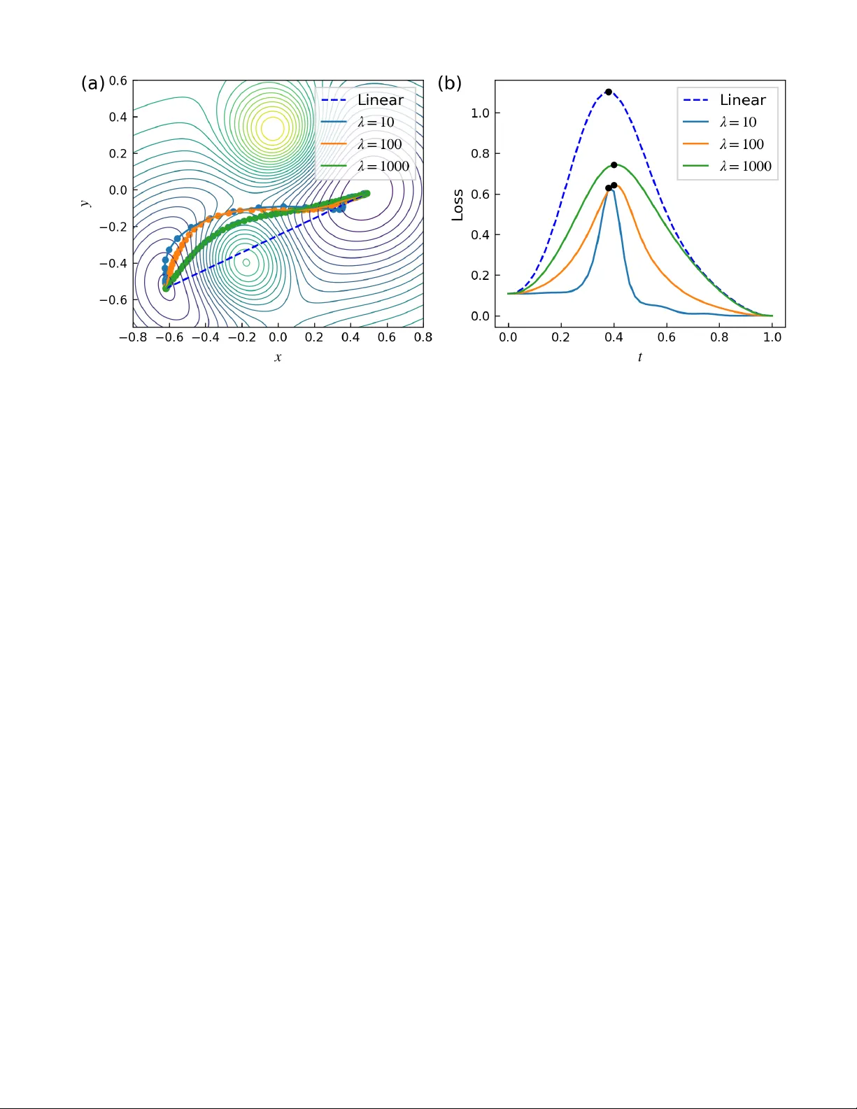
Neural net w ork optimization strategies and the top ograph y of the loss landscap e Jianneng Y u 1 and Alexandre V. Morozo v 1 , ∗ 1 Dep artment of Physics & Astr onomy, Rutgers, The State University of New Jersey, 136 F relinghuysen R d., Pisc ataway, NJ 08854, U.S.A. Neural net works are trained b y optimizing m ulti-dimensional sets of fitting parameters on non- con vex loss landscapes. Lo w-loss regions of the landscap es corresp ond to the parameter sets that p erform w ell on the training data. A key issue in mac hine learning is the p erformance of trained neural netw orks on previously unseen test data. Here, w e in vestigate neural netw ork training by sto c hastic gradient descen t (SGD) - a non-con vex global optimization algorithm whic h relies only on the gradient of the ob jectiv e function. W e contrast SGD solutions with those obtained via a non- sto c hastic quasi-Newton method, which utilizes curv ature information to determine step direction and Golden Section Search to choose step size. W e use sev eral computational to ols to inv estigate neural net work parameters obtained b y these t wo optimization methods, including kernel Principal Comp onen t Analysis and a nov el, general-purp ose algorithm for finding low-heigh t paths b etw een pairs of p oints on loss or energy landscap es, F ourierPathFinder. W e find that the choice of the optimizer profoundly affects the nature of the resulting solutions. SGD solutions tend to b e separated b y low er barriers than quasi-Newton solutions, even if b oth sets of solutions are regularized by early stopping to ensure adequate p erformance on test data. When allo wed to fit extensively on the training data, quasi-Newton solutions o ccup y deeper minima on the loss landscapes that are not reached by SGD. These solutions are less generalizable to the test data how ever. Ov erall, SGD explores smooth basins of attraction, while quasi-Newton optimization is capable of finding deep er, more isolated minima that are more spread out in the parameter space. Our findings help understand b oth the top ography of the loss landscap es and the fundamental role of landscap e exploration strategies in creating robust, transferrable neural netw ork mo dels. I In tro duction The problem of finding maximum or minimum v alues of multi-dimensional functions with complex non-linear structure arises in engineering, economic and financial forecasting, biological data analysis, molecular ph ysics, rob ot design, and numerous other scien tific and tec hnological settings. Notable examples include finding free energy minima in computer sim ulations of protein folding [ 1 , 2 ], conv erging to high-fitness states in ev olving p opulations [ 3 – 5 ], and minimizing loss functions in training neural netw orks [ 6 , 7 ]. Mo dern optimization algorithms used in deep learning [ 8 , 9 ] are p o werful enough to drive neural net work (NN) training loss to v ery low v alues across a wide v ariet y of NN architectures and training datasets. How ev er, minimiz- ing training error do es not necessarily guarantee robust p erformance on unseen data [ 10 ]. One reason for this is the possibility of ov erfitting in ov erparameterized deep NNs, which is t ypically mitigated by early stopping, weigh t regularization, and other techniques [ 6 , 7 ]. Some sets of trained NN parame ters generalize well, while others, despite ac hieving equally low training loss, fail to transfer, resulting in po or test accuracy [ 11 ]. This b eha vior underscores a central challenge in deep learning: understanding why some mo dels generalize while others do not, even if they o ccup y low-loss regions of the training landscap e. A k ey open question in deep learning theory is ho w differen t training pro cedures influence the t ypes of solutions found and the relative p ositions of these solutions on the loss landscap e; a related area of inquiry fo cuses on the loss landscap e top ography and connectivit y [ 12 – 14 ]. F or highly non-linear systems such as neural net works, the loss surface is thought to be comp osed of numerous basins of attraction connected by relatively flat v alleys [ 14 , 15 ]. Interestingly , ev en linear interpolation b etw een trained mo dels can reveal k ey features of the loss landscap e geometry , including the top ography of barriers and v alleys b et w een lo cal minima [ 16 ]. Later work addressed loss landscap e visualization with a v ariet y of computational to ols, establishing a dep endence of the loss landscap e curv ature around optimized solutions on the training metho d used in the optimization [ 17 ]. It has been widely observed that sto chastic gradien t descent (SGD) with small batch sizes tends to conv erge to flatter minima, which are often asso ciated with b etter generalization p erformance [ 11 , 14 , 15 ]. In contrast, adaptive metho ds lik e Adam [ 7 , 18 ] and RMSProp [ 7 , 19 ], though p oten tially faster in conv ergence and low er in training loss, ∗ morozov@ph ysics.rutgers.edu 2 frequen tly lead to sharp er solutions that ma y generalize less effectively [ 20 ]. Other methods that rely on curv ature information can achiev e even low er training loss, but are also known to conv erge to sharp er minima [ 21 ]. These observ ations prompt fundamental questions: do approaches that rely solely on the gradient information, suc h as SGD, find solutions in the same broad region of parameter space, or do they pro duce qualitativ ely distinct minima with v arying generalization prop erties? Are there significant differences b et w een solutions found by gradient vs. quasi-Newton metho ds [ 8 , 22 ] which rely on the curv ature information? Addressing these questions is crucial for understanding ho w optimization algorithms explore high-dimensional, non-conv ex loss landscap es which hav e to b e tra versed in NN training. Sev eral studies hav e recen tly examined the structure of NN loss landscap es and diversit y , connectivity , and gen- eralizabilit y of optimized solutions. F or instance, the distribution of Hessian eigenv alues during training was found to hav e significant v ariation across optimization strategies [ 23 ], suggesting that different metho ds may settle into differen t types of lo w-loss regions. It w as argued that the minima of the loss function are connected by low-heigh t paths [ 24 , 25 ], consistent with high levels of connectivity and contin uit y on the loss landscap es. F urthermore, it w as demonstrated that loss landscap es in deep neural netw orks admit star-con vex paths b etw een initial states and optimized solutions, allowing gradien t-based metho ds such as SGD to av oid lo cal kinetic traps [ 26 ]. Sets of optimized solutions in ov erparameterized netw orks frequen tly form star domains, whic h are regions where any p oin t can b e connected to a ‘central’ solution via low-loss paths [ 27 ]. In this work, we fo cus on the relative adv an tages and disadv an tages of employing SGD, a widely used stochastic gradien t-based optimizer [ 7 ], versus an efficient quasi-Newton metho d, Limited-memory Bro yden-Fletcher-Goldfarb- Shanno [ 8 , 28 – 31 ], augmen ted with a Golden Section Search for determining the step size (L-BFGS-GSS). W e find that although b oth methods yield similar p erformance on test data when early stopping is employ ed for regularization, the solutions found b y the tw o optimizers are qualitatively differen t. The L-BFGS-GSS s olutions are separated by higher barriers and are more distan t from one another in parameter space. L-BF GS-GSS optimization can lead to v ery low training loss v alues compared to SGD, resulting in ov erfit, p o orly generalizable solutions. In contrast, SGD solutions are more generalizable, in agreemen t with previous studies [ 11 , 14 , 15 ]. T o study SGD and L-BFGS-GSS solutions sets, w e dev elop a num b er of approaches aimed at their visualization in the con text of the loss landscap e top ograph y , including a nov el algorithm for finding low-heigh t paths connecting pairs of p oints on loss, energy , or negativ e fitness landscap es, FourierPathFinder . I I Metho ds A Neural Net w ork Arc hitectures W e study the loss landscap es of four neural netw ork (NN) architectures trained on the MNIST dataset of 28 × 28 blac k-and-white images of handwritten digits [ 32 ]. The first NN we consider is a fully connected p erceptron (FCP) – a feedforw ard net work with tw o hidden lay ers of 50 units each, which use ReLU activ ations and no bias terms. The input lay er has 784 no des and receiv es D = 28 × 28 = 784 pixel v alues as inputs; the output lay er is a softmax classifier into 10 single-digit classes: 0 . . . 9. The second NN is a c on v olutional neural net work (CNN) [ 33 ] with LeNet arc hitecture [ 34 ]. It consists of tw o conv olutional la yers with 6 and 16 channels, resp ectively , eac h follow ed by av erage p ooling and ReLU activ ation. The tw o-lay er conv olutional blo ck is follo wed by three fully connected lay ers with 120, 84, and 10 no des; the last lay er outputs probabilities of 10 single-digit classes. The third NN is a Long Short-T erm Memory (LSTM) recurren t net w ork [ 35 ]. F ollowin g Ref. [ 36 ], each image is flattened and p erm uted o ver all 784 pixels (with a fixed random seed for repro ducibilit y), then reshap ed in to 28 time steps of 28 features eac h for the sequen tial pro cessing b y the LSTM. The LSTM has a hidden lay er size of 48 and outputs the final hidden state to a linear classifier with 10 output units and no bias term. Finally , we emplo y a shallo w auto encoder architecture [ 37 ] to explore unsupervised loss landscap es. The enco der and deco der each consist of t wo FC lay ers with 32 units p er lay er, softplus activ ations, and no biases; the final la yer of the deco der uses a sigmoid activ ation to reconstruct the image. Implemen tations of all four NN model architectures are av ailable at https://github.com/jy856-jpg/path-finding . The total n umber of fitting parameters for eac h NN, N prm , is listed in T able I . F or the three classification mo dels, we define the loss function ⟨ l ( x train , ω ) ⟩ or ⟨ l ( x test , ω ) ⟩ as the cross-entrop y loss betw een the predicted output and the true lab el, a veraged ov er the en tire training or test set (except for SGD optimization, where the a verages are taken o v er 64 images in a mini-batch). F or the auto enco der, ⟨ l ( x train , ω ) ⟩ or ⟨ l ( x test , ω ) ⟩ is defined as the mean squared reconstruction error, also av eraged ov er the entire training or test set. Here, ω denotes a vector of mo del-dep enden t w eights and biases. W e use a standard split of the MNIST dataset into { x train } with N = 5 × 10 4 training images and { x test } with N = 10 4 test images [ 32 ]. 3 B Quasi-Newton optimization with Golden Section Searc h Second-order optimization methods aim to improv e con v ergence by incorp orating curv ature information [ 22 , 38 ]. The function to b e minimized is approximated lo cally using a second-order T aylor expansion: f ( z + ϵ ) ≈ f ( z ) + ∇ f ( z ) T ϵ + 1 2 ϵ T H ϵ, (1) where f ( z ) is a function of an N -dimensional argument z , ∇ f ( z ) = ∇ y f ( y ) | y = z represen ts its gradien t ev aluated at z ( ∇ y = ∂ /∂ y 1 . . . ∂ /∂ y N ), and H is the Hessian matrix of second deriv ativ es: H ij = ∂ 2 f ( y ) /∂ y i ∂ y j | y = z ( i, j = 1 . . . N ). In the Newton-Raphson iterative optimization metho d, the up date step is given b y [ 22 ]: z new = z old − H − 1 ∇ f ( z ) . (2) Note that b oth the direction and the magnitude of the minimization step are determined by the in verse of the Hessian matrix – there is no need to choose the step size as in first-order optimization metho ds that rely solely on the gradien ts [ 7 ]. How ev er, computing and inv erting the Hessian matrix scales p o orly with the num b er of parameters [ 22 , 39 ], whic h makes it infeasible to apply Eq. ( 2 ) to large models such as deep neural net w orks. T o mitigate the high computational cost of second-order metho ds, quasi-Newton algorithms suc h as Limited-memory Bro yden-Fletcher- Goldfarb-Shanno (L-BFGS) [ 8 , 28 – 31 ] are used to approximate the pro duct b etw een the inv erse Hessian and the gradien t without explicitly computing and in verting the Hessian matrix. After computing the search direction p = H − 1 ∇ f ( z ), a line search is typically carried out to find the optimal step size, using Armijo-W olfe conditions or other suitable criteria [ 8 , 40 ]. In the NN context, the goal is to optimize f ( ω ) = ⟨ l ( x, ω ) ⟩ , where l ( x, ω ) denotes the loss function corresp onding to the input datapoint x (in our case, a single MNIST image) at the current set of weigh ts ω , and the a verage is tak en ov er all images in the training dataset. Note that N = N prm in this case (cf. T able I ). Here, we use the Golden Section Search (GSS) [ 38 ] – a light w eigh t and deriv ativ e-free approac h to line search. The goal of GSS, as in an y line searc h algorithm, is to find an optimal step size u along the searc h direction p by minimizing f ( u ) = ⟨ l ( x, ω − up ) ⟩ , where f ( u ) is now a 1D function. Briefly , GSS is used to find the minim um of a unimo dal 1D function on a closed in terv al by rep eatedly shrinking a brac ket that contains the minimum. A t each step, the in terv al is reduced by a fixed fraction determined by the golden ratio ϕ = (1 + √ 5) / 2, allowing one function ev aluation to b e reused, so that only a single new ev aluation is needed p er iteration. The algorithm con v erges robustly and linearly , with the error decreasing by a constant factor at each iteration. W e call the L-BFGS algorithm augmented by GSS the L-BFGS-GSS optimizer, summarized in Algorithm 1 . Note that our customized implemen tation of the L-BF GS optimizer main tains t w o lists of size m , s list and y list , that con tain m most recent differences s k = ω k − ω k − 1 and y k = ∇ f ( ω k ) − ∇ f ( ω k − 1 ), resp ectiv ely . Algorithm 1: Ov erview of the L-BF GS-GSS optimizer. Input: Ob jectiv e function f ( ω ) = ⟨ l ( x, ω ) ⟩ , initial NN parameters ω 0 , maximum num b er of iterations K , training data x Output: Optimized NN parameters ω ⋆ for k = 1 to K do Compute gradient, ∇ f ( ω k ) Compute search direction p ( ∇ f ( ω k ) , s list , y list ) via L-BFGS Determine optimal step size u ⋆ with GSS, such that f ( ω k − u ⋆ p ) is minimized ω k +1 ← ω k − u ⋆ p Up date s list , y list return ω ∗ ← ω K +1 C Construction of lo w-loss paths b et w een t w o p oints on the landscap e W e hav e developed a general-purp ose path-finding algorithm, called FourierPathFinder (Algorithm 2 ), which constructs low-loss paths betw een tw o p oin ts on a multi-dimensional landscap e as a combination of a straight line and a truncated F ourier series: ω ( t ) = tω i + (1 − t ) ω j + N F X n =1 b n sin( nπ t ) , (3) 4 where ω i and ω j are the initial and final p oints on the landscap e, t ∈ [0 , 1] is the curve parameter, and N F is the total num b er of F ourier terms (w e typically set N F = 10). The F ourier co efficients b n are initialized to 0. F or NN loss landscap es, w e discretize the curv e parameter t in to M = 50 equally spaced v alues. The total loss along the path in Eq. ( 3 ) is computed as: L ( ω i , ω j ) = M X m =1 ⟨ l ( x, ω ( t m )) ⟩ + λ M − 1 X m =1 | ω ( t m +1 ) − ω ( t m ) | 2 , (4) where the first term is the cumulativ e loss along the path. The second term is a regularization p enalty , scaled by the hyperparameter λ which con trols the smo othness and the non-linearity of the path. W e choose λ = 10 − 4 for the paths on NN loss landscap es – we find that this v alue provides a reasonable balance betw een the total path length and the cumulativ e loss along the path. Algorithm 2: Ov erview of the FourierPathFinder algorithm. Input: P ath loss function L ( ω i , ω j ) (Eq. ( 4 )), maximum n umber of iterations K , input data { x } , curve parameter v alues { t m } M m =1 , regularization co efficient λ , F ourier co efficien ts { b n } N F n =1 initialized to 0. Output: Optimized F ourier co efficien ts { b ⋆ n } N F n =1 . for k = 1 to K do Compute NN loss gradients with resp ect to NN parameters at eac h t m : g m ( x ) = ∂ ⟨ l ( x,ω ) ⟩ ∂ ω | ω = ω ( t m ) Compute the path loss gradien t with resp ect to the F ourier co efficients: ∂ L ∂ b n = P M m =1 g m ( x ) sin( nπ t m ) + 2 λ P M − 1 m =1 [ ω ( t m +1 ) − ω ( t m )][sin( nπ t m +1 ) − sin( nπ t m )] Up date { b n } N F n =1 using Adam optimizer [ 18 ] on the entire dataset { x } return { b ⋆ n } N F n =1 ← { b n } N F n =1 T o c haracterize barrier height along a given path, we compute path height, defined as the maxim um loss encoun tered along the discretized tra jectory: H = max t m {⟨ l ( x, ω ( t m )) ⟩} . (5) D Dimensionalit y reduction for c haracterizing optimized NN parameter s ets T o visualize the training or test sets of NN parameters optimized using either L-BFGS or SGD, we employ a dimensionalit y reduction tec hnique called kernel Principal Comp onent Analysis (kPCA) [ 22 , 41 ]. Briefly , kPCA is a nonlinear generalization of standard PCA, a linear dimensionality reduction metho d designed to identify orthogonal directions (principal comp onents) along which the data v aries most [ 22 ]. kPCA extends this approach to capture nonlinear structures in the data by implicitly mapping input datap oints x ∈ R D in to a feature space ϕ ( x ) ∈ R M through nonlinear mapping x → ϕ ( x ). The similarity b etw een tw o p oin ts x and x ′ in the feature space is expressed through a kernel function k ( x, x ′ ) = ϕ ( x ) T ϕ ( x ′ ), which computes the inner pro duct b et w een their feature-space representations. Common k ernel functions include the linear k ernel k ( x, x ′ ) = x T x ′ , the degree n p olynomial k ernel k ( x, x ′ ) = ( x T x ′ + C ) n , and the radial basis function (RBF) kernel k ( x, x ′ ) = exp ( −| x − x ′ | 2 / 2 σ 2 ), each defining a different notion of similarity b etw een datap oin ts x and x ′ . Eac h kernel corresp onds to a p otentially infinite-dimensional set of feature vectors. Note also that k ernels often dep end on hyperparameters suc h as C in the polynomial or σ in the RBF kernel. W e set 2 σ 2 = N prm in visualizing optimized vectors of NN weigh ts and biases. As is t ypical in kernel-based metho ds, kPCA a voids constructing the feature vectors explicitly – the dimensionalit y reduction is carried out using the k ernel matrix K ∈ R N × N , where K ij = k ( x i , x j ) and N is the n umber of datapoints. Sp ecifically , the kernel matrix is cen tralized [ 22 ]: K → e K , where the centralized k ernel corresp onds to the feature v ectors with zero mean: e K ij = e k ( x i , x j ) = e ϕ ( x i ) T e ϕ ( x j ), with P N n =1 e ϕ ( x n ) = 0. Next, the eigenv alues and eigenv ectors of the N × N centralized kernel matrix are found by solving the eigenv alue problem: e K α ( k ) = λ ( k ) α ( k ) . Finally , the principal comp onent pro jections are computed using PC k ( x ) = P N i =1 α ( k ) i k ( x, x i ), where k lab els the eigenv alues and x is the input v ector to b e pro jected. 5 I I I Results A Ov erview of NN optimization and loss landscap e visualization Our approac h to NN training and loss landscape exploration is outlined in Figure 1 . W e train four NN arc hitectures (F CP , LeNet CNN, Auto enco der, and LSTM) on a set of MNIST images [ 32 ] using tw o algorithms: Sto c hastic Gradien t Descent (SGD) [ 39 ] with 64 images p er mini-batch and a customized quasi-Newton algorithm, L-BFGS-GSS (Metho ds). W e obtain sets of optimized NN parameters lo cated in low-loss regions of the multi-dimensional loss landscap es and study the depths of these minima, their basins of attraction, and the heights of the barriers separating optimized parameter vectors from one another. Figure 1: Generation and visualization of optimized NN parameter sets. (a) A subset of input training/test data. A single 28 × 28 MNIST image [ 32 ] is used as NN input. (b) Representativ e NN architecture, with an input lay er, tw o hidden lay ers, and an output lay er. (c) A conceptual sketc h of the corresp onding NN loss landscap e, with tw o lo cal minima (red dots) lo cated in a shallow v alley . The basins of attraction of the tw o minima are separated by a relativ ely low barrier. Sp ecifically , we assem ble four sets of optimized parameters for each of the four NN architectures considered in this w ork: FCP , LeNet CNN, Auto enco der, and LSTM (see Metho ds for NN implementation details). All neural nets employ O (10 4 ) fitting parameters (T able I ). The first t wo sets, { ω train ,i BFGS } 48 i =1 and { ω test ,i BFGS } 48 i =1 , corresp ond to the solutions obtained using the L-BFGS-GSS quasi-Newton algorithm without mini-batc hes (Algorithm 1 ; see Metho ds for details). The second tw o sets, { ω train ,i SGD } 48 i =1 and { ω test ,i SGD } 48 i =1 , comprise solutions obtained using SGD [ 9 , 42 ] with 64-image mini-batches. Eac h NN mo del is trained starting from 75 different random initializations of w eights and biases for each optimizer type; 48 solutions with the low est training loss from each metho d are selected to form { ω train ,i BFGS } 48 i =1 and { ω train ,i SGD } 48 i =1 . T o obtain the corresp onding test set fitting weigh ts, { ω test ,i BFGS } 48 i =1 and { ω test ,i SGD } 48 i =1 , we emplo y early stopping at the minimum of test loss for the mo dels included into our training sets [ 7 ]. Figure 2 sho ws a representativ e example of training/test L-BF GS-GSS and SGD loss curves for the LSTM netw ork (loss curves for the other three architectures are display ed in Fig. S1 ). The training or test optimized NN parameter sets corresp ond to the minimum of the corresp onding loss curve. T able I shows the a verage loss ov er 48 indep enden t runs. F or all NN architectures, the v alues of the a v erage training loss are considerably low er for the L-BF GS-GSS optimizer compared to SGD. How ev er, the a verage test loss v alues are comparable, indicating that the L-BF GS-GSS training weigh ts are likely to be ov erfit. Note also that the L-BFGS-GSS test loss curves rise sharply from the minima in all NN arc hitectures except the auto enco der (cf. blue lines in Figs. 2 b and S1 b,d,f ). In contrast, SGD weigh t sets app ear to b e more generalizable. 6 Figure 2: LSTM loss curves . Representativ e LSTM training (a) and test (b) loss curves ( ⟨ l ( x train , ω ) ⟩ and ⟨ l ( x test , ω ) ⟩ , resp ectively) as a function of the num b er of ep o c hs. In b oth panels, dashed vertical lines mark the ep ochs where the loss curves of the same color reach their minima. The weigh t configurations ω train SGD , ω test SGD and ω train BFGS , ω test BFGS denote the sets of NN parameters found at these minima (optimized with SGD and L-BFGS-GSS, resp ectiv ely). T able I: Average training and test loss. F or each NN architecture, we list the training loss ⟨ l ( x train , ω train ) ⟩ and the test loss ⟨ l ( x test , ω test ) ⟩ av eraged o ver 48 indep endent runs. Also listed are N prm , the total num b er of NN fitting parameters (weigh ts and biases) in each of the four architectures. ⟨ l ( x train , ω train ) ⟩ ⟨ l ( x test , ω test ) ⟩ NN L-BF GS SGD L-BF GS SGD N prm F CP 1.26e-08 6.21e-04 9.69e-02 8.25e-02 42200 LeNet 3.35e-08 1.76e-05 4.17e-02 3.89e-02 61706 Auto encoder 1.69e-02 4.57e-02 1.65e-02 4.52e-02 52224 LSTM 1.63e-06 1.35e-02 1.55e-01 1.28e-01 15456 B Lo w-loss paths connecting optimized states on NN loss landscap es W e hav e developed FourierPathFinder , an algorithm for finding low-heigh t paths connecting t wo points on multi- dimensional loss or energy landscap es (Algorithm 2 ; see Metho ds for implementation details). Figure 3 a illustrates our algorithm on a synthetic 2D landscap e f ( x, y ) with tw o lo cal minima – shown are a linear path b etw een the t wo minima and three paths found using FourierPathFinder with increasing regularization p enalties: λ = 10 , 100 , 1000. Figure 3 b traces the corresp onding loss v alues along these paths, given here by the v alues of f ( x, y ) along eac h parametrized curve. W e observe that all three optimized paths find a low-loss v alley b etw een tw o neigh boring maxima. How ev er, the length of the λ = 10 path is not suffic ien tly constrained, enabling it to sp end more time in the low-loss regions around the tw o minima and make larger steps in crossing the barrier betw een the t wo basins of attraction (cf. the spacing of the blue p oints in Fig. 3 a and the loss profile for the λ = 10 curv e in Fig. 3 b). Larger v alues of λ preven t this non-uniform b eha vior and result in more regular paths. Despite these differences, the maximum heigh t along the path (Eq. ( 5 )) is fairly insensitiv e to λ . Thus, there is no need to fine-tune this hyperparameter. Next, we consider the heights of the paths connecting optimized vectors of parameters on the NN loss landscap es. F or eac h of the four sets con taining 48 vectors of trained parameters, we randomly c ho ose 300 pairs of vectors and use FourierPathFinder (with λ = 10 − 4 ) to find the lo w-loss paths connecting them. W e record the corresponding 7 Figure 3: Lo w-loss paths on a 2D landscap e. (a) Two-dimensional loss landscap e comp osed of tw o p ositive and t wo negative Gaussian p eaks: f ( x, y ) = − P 2 i =1 exp[ − 3 | r − c i | 2 ] + P 2 j =1 exp[ − 15 | r − d j | 2 ] + C , where r = ( x, y ), c 1 = ( − 0 . 5 , − 0 . 5), c 2 = (0 . 5 , 0 . 0), d 1 = ( − 0 . 2 , − 0 . 4), d 2 = (0 . 0 , 0 . 3), and C = 1 . 019. F our representativ e paths connecting tw o landscape minima: w 1 = ( − 0 . 62 , − 0 . 54) and w 2 = (0 . 49 , − 0 . 02) are sho wn: a linear interpolation path (dashed blue line) and three FourierPathFinder optimized paths ( λ = 10, solid blue curve; λ = 100, solid orange curve; λ = 1000, solid green curve). Dots indicate function v alues at discrete time steps t m ∈ [0 , 1] along the path: f ( x ( t m ) , y ( t m )), m = 1 . . . M ( M = 100). (b) Loss v alues f ( x ( t ) , y ( t )) as a function of the curve parameter t along the four paths in panel (a): the linear interpolation path (dashed blue curve) and three FourierPathFinder paths (solid curves with the colors matching the paths in panel (a)). Path heights H i (Eq. ( 5 )) are lab eled with blac k dots, with H 0 = 1 . 102 (straight line), H 1 = 0 . 646 (optimized path, λ = 10), H 2 = 0 . 640 (optimized path, λ = 100), and H 3 = 0 . 652 (optimized path, λ = 1000). path heights (Eq. ( 5 )), whic h characterize the connectivity of optimized v ectors ω in the parameter space. W e find that, with the exception of Auto enco der, the barrier heights are low er for the SGD solutions compared to BF GS. This is true for b oth { ω test ,i SGD } 48 i =1 and { ω train ,i SGD } 48 i =1 on the training landscap e (Fig. 4 ) and { ω test ,i SGD } 48 i =1 on the test landscape (Fig. S2 ). This indicates that SGD solutions are located in smo other, more accessible regions of the loss landscape. In contrast, BFGS solutions { ω test ,i BFGS } 48 i =1 and { ω train ,i BFGS } 48 i =1 are c haracterized by higher barriers on b oth landscapes, indicating that those vectors of optimized parameters are more isolated from one another. Note that Auto encoder is probably an exception b ecause it do es not exhibit strong BFGS o v erfitting prominent in the other three NN architectures (Fig. S1 , T able I ). In terestingly , on the training landscap e the BFGS barrier heights b etw een vectors of training weigh ts are only higher than the barrier heights b etw een v ectors of test weigh ts in tw o out of four NN architectures, FCP and LSTM (cf. navy blue and light blue histograms in Fig. 4 ). This is surprising b ecause BFGS training weigh ts are ov erfit for F CP , LeNet, and LSTM (T able I ). In other words, the L-BFGS-GSS optimizer do es not necessarily find more isolated minima with additional training, even if o verfitting o ccurs. Although the same observ ation is true for SGD (cf. light red and gold histograms in Fig. 4 ), it is less surprising there due to muc h weak er signatures of ov erfitting in the case of SGD optimization. C Statistics of optimized NN parameters In addition to the analysis of the paths connecting pairs of optimized v ectors of NN parameters, we consider the statistics of optimized NN weigh ts and biases. T o this end, w e compute the means and standard deviations of the comp onen ts of W train,j BFGS , W test,j BFGS , W train,j SGD , W test,j SGD v ectors, where each W v ector is constructed by concatenation of the corresponding { ω i } 48 i =1 set of vectors and j = 1 . . . 4 lab els NN architectures (T able S1 ). W e see that there is a clear difference b etw een SGD and BFGS w eigh ts, with the latter characterized by larger standard deviations σ . Thus, BF GS fitting weigh ts tend to b e more spread out in parameter space. 8 Figure 4: Distribution of barrier heights along optimized paths on the training landscape. Shown are distributions of the FourierPathFinder path heights (Eq. ( 5 )) for F CP (a), LeNet (b), Auto encoder (c), and LSTM (d). Histograms in each panel show heigh ts of 300 low-loss paths connecting randomly chosen pairs of optimized parameter vectors in { ω train ,i BFGS } 48 i =1 (na vy blue), { ω test ,i BFGS } 48 i =1 (ligh t blue), { ω train ,i SGD } 48 i =1 (ligh t red), and { ω test ,i SGD } 48 i =1 (gold). The paths are computed on the training landscap e, ⟨ l ( x train , ω ) ⟩ . Another wa y to see the extent of the spread is to compare the L 2 lengths of the SGD and BFGS weigh t vectors. W e fo cus first on the comparison betw een SGD test and BF GS training weigh ts since the latter are ov erfit (except in the Auto enco der; Figs. 2 and S1 , T able I ), enabling us to con trast SGD w eight sets that one w ould use in practice with low-loss, non-generalizable solutions obtained by L-BFGS-GSS. Sp ecifically , w e define ¯ ω BFGS = 1 48 P 48 i =1 ω test ,i BFGS and ¯ ω SGD = 1 48 P 48 i =1 ω test ,i SGD as the cen troids of the optimized w eight vector sets and use ¯ ω = 1 2 ( ¯ ω BFGS + ¯ ω SGD ) as the common origin of all weigh t v ectors. F or each individual weigh t vector ω i , we calculate its L 2 distance from the origin as | ω i − ¯ ω | . The histogram of L 2 distances shows that, as exp ected from T able S1 , BFGS weigh t vectors tend to b e longer than SGD weigh t v ectors (Fig. 5 ). This indicates that optimized weigh t v ectors found by L-BF GS-GSS are more widely disp ersed compared to the SGD solutions, which form a more compact distribution. The distance b etw een ¯ ω BFGS and ¯ ω SGD is small compared to the spread of v ector lengths within each group (cf. vertical dotted lines in Fig. 5 ), indicating that there is no strongly preferred direction in the parameter space. Next, we consider SGD and BF GS test weigh ts, as those are the w eight vector sets one w ould use in practice (Fig. S3 ). W e observ e that, as might b e exp ected, the SGD and BFGS vector lengths b ecome less different for FCP and LeNet. Surprisingly , the gap b etw een v ector length histograms remains nearly the same for Autoenco der and LSTM, despite the latter being ov erfit in going from test to training w eight sets. D Lo w-dimensional pro jections of optimized weigh t v ectors W e chec k ed whether the differences b etw een BFGS training and SGD test weigh t vectors can b e detected using principal comp onent analysis (PCA) – a dimensionality reduction technique often used in data visualization [ 22 ]. Sp ecifically , w e hav e applied kernel PCA (kPCA; see Metho ds for details) to { ω train ,i BFGS } 48 i =1 and { ω test ,i SGD } 48 i =1 sets of 9 Figure 5: Distributions of SGD test and BF GS training weigh t vector lengths. Shown are the histograms of L 2 distances b et ween individual weigh t vectors ω i and the common origin ¯ ω , | ω i − ¯ ω | . Distributions of the BFGS training ( { ω train ,i BFGS } 48 i =1 ) and SGD test ( { ω test ,i SGD } 48 i =1 ) weigh t v ector lengths are plotted in blue and light red, resp ectiv ely , for FCP (a), LeNet (b), Auto enco der (c), and LSTM (d). Dotted vertical lines indicate the p ositions of | ¯ ω BFGS − ¯ ω | = | ¯ ω SGD − ¯ ω | . optimized w eigh t v ectors for each NN arc hitecture (Fig. 6 ). In all four cases, w e see clear separation of BF GS and SGD v ectors pro jected on to tw o first principal components PC 1 and PC 2 . In terestingly , the separation is predominan tly along the first principal comp onent, indicating that the BF GS and SGD weigh t vectors form tw o distinct clusters in the parameter space. Moreov er, the separation is only observ ed with the RBF k ernel and disapp ears when other k ernels suc h as polynomial and sigmoid are used, or when standard PCA is employ ed (data not shown). Th us, the separation is radial rather than along a preferred direction, consisten t with the larger BF GS vector lengths and the absence of preferred directions in Fig. 5 . When kPCA is applied to BF GS and SGD test weigh t vectors (Fig. S4 ), cluster separation nearly disapp ears for F CP and LeNet but p ersists for Auto enco der and LSTM, in agreement with Fig. S3 . IV Discussion and Conclusion The results presented here demonstrate that the balance betw een generalization and ov erfitting profoundly influences the nature of optimized neural netw ork solutions. Consistent with previous observ ations [ 11 , 20 , 21 ], we find that SGD pro duces more generalizable solutions that o ccupy flatter, more connected basins of the loss landscap e, whereas L-BF GS-GSS solutions consist of sharp er, more isolated minima separated by higher barriers. The latter b eha vior is particularly pronounced if the L-BFGS-GSS optimizer is allow ed to ov erfit, conv erging to solutions which ha ve muc h lo wer loss compared to SGD (T able I ). These observ ations are confirmed b y the analysis of the paths connecting pairs of optimized weigh t vectors in m ulti-dimensional parameter space. W e hav e developed a nov el algorithm, FourierPathFinder , which uses a F ourier expansion of paths combined with sto c hastic gradien t optimization to find low-heigh t paths b etw een tw o points on 10 Figure 6: kPCA pro jections of SGD test and BF GS training w eigh t v ectors. Shown are the first tw o principal comp onen ts, PC 1 and PC 2 , obtained by kPCA with the RBF kernel (Metho ds). The pro jections are applied to { ω train ,i BFGS } 48 i =1 (blue p oin ts) and { ω test ,i SGD } 48 i =1 (red p oin ts) sets of optimized weigh t vectors, for FCP (a), LeNet (b), Auto enco der (c), and LSTM (d). arbitrary loss or energy landscap es. W e find that SGD solutions are typically separated by low er energy barriers than those obtained with L-BFGS-GSS (Figs. 4 , S2 ). The lo wer barrier heights encountered along SGD paths suggest that SGD solutions tend to lie in broad, smo othly connected v alleys of the loss surface, whereas L-BFGS-GSS solutions app ear to b e em b edded in steep er, more difficult-to-na vigate regions. Thus, our path analysis supp orts the view that SGD tends to conv erge to flatter minima, a hallmark of b etter generalization, while L-BF GS-GSS, a quasi-Newton metho d guided by curv ature information, is more prone to settling in narrow, high-curv ature basins that fit the training data very well but generalize p o orly . This interpretation is reinforced b y the analysis of the lengths of optimized weigh t vectors (Figs. 5 , S3 ; T able S1 ). SGD solutions cluster more compactly near a common centroid, while L-BF GS-GSS solutions are distributed farther from the cen ter, forming a larger-radius shell in parameter space. There app ear to be no strongly preferred directions within the SGD and BFGS shells – the main difference is in the vector lengths, explained at least in part by the larger magnitudes of BFGS vector comp onents (T able S1 ). Interestingly , the centroids of the SGD and BFGS weigh t v ectors are relatively close to one another, supp orting the idea of a nested, shell-like organization of SGD and BFGS w eight vectors in the parameter space. F urther evidence of these structural differences emerges from visualization of multi-dimensional weigh t vectors 11 based on kPCA pro jections (Figs. 6 , S4 ). kPCA analysis with a spherically symmetric, non-linear RBF kernel reveals clear separation b etw een the solution sets pro duced by SGD and L-BFGS-GSS, esp ecially when the latter algorithm is allow ed to ov erfit. This observ ation implies that the tw o optimizers conv erge to distinct, nonlinearly separable manifolds in parameter space rather than to nearby p oin ts within a single connected region. T ak en together, our results show that SGD solutions o ccup y relativ ely compact, flatter regions of the loss landscap e, while L-BFGS-GSS solutions concentrate within a larger-diameter shell corresp onding to higher-curv ature, less acces- sible minima. This radial organization supp orts the idea that sto c hastic gradient based methods tend to find central, robust basins in parameter space, while deterministic quasi-Newton metho ds conv erge tow ard more spread-out, less generalizable minima. Th us, the choice of the optimizer affects not only con v ergence speed but also the qualitative nature of the resulting solutions. The differences b et ween SGD and L-BFGS-GSS reflect fundamentally different optimization dynamics that guide eac h metho d tow ard distinct regions of the loss landscap e. In practical terms, smoother connectivit y b etw een SGD minima facilitates mo del av eraging and transfer compared to the L-BF GS-GSS approac h. More broadly , the low-barrier connectivity , compact clustering, and nonlinear separability of generalizable solutions pro vide a geometric foundation for understanding wh y flatter minima, fa vored b y SGD, tend to yield more robust performance in neural net works. In summary , our findings underscore ho w optimizer c hoice in mac hine-learning con texts affects not only the efficiency of con v ergence to low-loss solutions, but also the geometry and diversit y of the solutions themselves – with p oten tial consequences for generalization and robustness. Soft w are and Data Av ailabilit y The neural netw ork training and loss landscap e analysis softw are was written in Python and is av ailable via GitHub at https://github.com/jy856-jpg/path-finding . Ac kno wledgmen ts J.Y. and A.V.M. ackno wledge financial and logistical support from the Cen ter for Quan titative Biology , Rutgers Univ ersity . The authors are grateful to the Office of Adv anced Research Computing (OAR C) at Rutgers Universit y for providing access to the Amarel cluster. [1] J. N. On uchic and P . G. W olynes, Theory of protein folding, Curr. Op. Struct. Biol. 14 , 70 (2004). [2] K. A. Dill, S. B. Ozk an, M. S. Shell, and T. R. W eikl, The protein folding problem, Ann. Rev. Biophys. 37 , 289 (2008). [3] J. F. Cro w and M. Kim ura, An Intro duction to Population Genetics The ory (Harp er and Ro w, New Y ork, NY, USA, 1970). [4] M. Kimura, The Neutr al The ory of Mole cular Evolution (Cambridge Univ ersity Press, Cambridge, UK, 1983). [5] J. Gillespie, Population Genetics: A Concise Guide (The Johns Hopkins Universit y Press, Baltimore, MD, USA, 2004). [6] I. Go o dfello w, Y. Bengio, and A. Courville, De ep L e arning (MIT Press, Cambridge, MA, USA, 2016). [7] P . Meh ta, M. Buk ov, C.-H. W ang, A. G. R. Day , C. Ric hardson, C. K. Fisher, and D. J. Sch w ab, A high-bias, low-v ariance in tro duction to Machine Learning for physicists, Ph ys. Rep. 810 , 1 (2019). [8] J. Nocedal and S. J. W righ t, Numeric al optimization (Springer Science+Business Media, LLC, New Y ork, NY, USA, 2006). [9] S. Ruder, An ov erview of gradient descent optimization algorithms (2017), arXiv:1609.04747 [cs.LG] . [10] C. Zhang, S. Bengio, M. Hardt, B. Rech t, and O. Vin yals, Understanding deep learning (still) requires rethinking general- ization, Commun. A CM 64 , 107 (2021) . [11] N. S. Kesk ar, D. Mudigere, J. No cedal, M. Smely anskiy , and P . T. P . T ang, On large-batc h training for deep learning: Generalization gap and sharp minima (2017), arXiv:1609.04836 [cs.LG] . [12] P . Chaudhari, A. Choromansk a, S. Soatto, Y. LeCun, C. Baldassi, C. Borgs, J. Chay es, L. Sagun, and R. Zecchina, En tropy-SGD: biasing gradient descent into wide v alleys, Journal of Statistical Mec hanics: Theory and Experiment 2019 , 124018 (2019) . [13] S. Jastrzebski, Z. Ken ton, D. Arpit, N. Ballas, A. Fisc her, Y. Bengio, and A. Storkey , Three factors influencing minima in SGD (2018), arXiv:1711.04623 [cs.LG] . [14] Y. F eng and Y. T u, The inv erse v ariance-flatness relation in sto chastic gradien t descent is critical for finding flat minima, Pro c. Nat. Acad. Sci. USA 118 , e2015617118 (2021). [15] M. W ei and D. J. Sch wab, Ho w noise affects the hessian sp ectrum in ov erparameterized neural net w orks (2019), arXiv:1910.00195 [cs.LG] . [16] I. J. Go o dfello w, O. Viny als, and A. M. Saxe, Qualitatively characterizing neural net work optimization problems (2015), arXiv:1412.6544 [cs.NE] . 12 [17] H. Li, Z. Xu, G. T aylor, C. Studer, and T. Goldstein, Visualizing the loss landscape of neural nets, in A dvanc es in Neur al Information Pr o c essing Systems , V ol. 31, edited by S. Bengio, H. W allac h, H. Laro chelle, K. Grauman, N. Cesa-Bianchi, and R. Garnett (Curran Asso ciates, Inc., 2018). [18] D. P . Kingma and J. L. Ba, Adam: A metho d for sto c hastic optimization (2014), arXiv:1412.6980 [cs.LG] . [19] T. Tieleman and G. Hinton, Lecture 6.5 – RMSProp: Divide the gradient by a running av erage of its recent magnitude, COURSERA: Neural Netw orks for Machine Learning (2012). [20] A. C. Wilson, R. Ro elofs, M. Stern, N. Srebro, and B. Rech t, The marginal v alue of adaptiv e gradient metho ds in mac hine learning, in Pr o c e e dings of the 31st International Conferenc e on Neur al Information Pr o c essing Systems , NIPS’17 (Curran Asso ciates Inc., Red Ho ok, NY, USA, 2017) pp. 4151–4161. [21] Z. Y ao, A. Gholami, K. Keutzer, and M. W. Mahoney , Hessian-based analysis of large batch training and robustness to adversaries, in Pr o c ee dings of the 32nd International Confer enc e on Neural Information Pr o c essing Systems , NIPS’18 (Curran Asso ciates Inc., Red Ho ok, NY, USA, 2018) pp. 4954–4964. [22] C. M. Bishop, Pattern r e c o gnition and machine learning (Springer Science+Business Media, LLC, New Y ork, NY, USA, 2006). [23] B. Ghorbani, S. Krishnan, and Y. Xiao, An inv estigation in to neural net optimization via Hessian eigenv alue density , in Pr o c e e dings of the 36th International Confer enc e on Machine L e arning , Proceedings of Mac hine Learning Research, V ol. 97, edited by K. Chaudhuri and R. Salakhutdino v (PMLR, 2019) pp. 2232–2241. [24] T. Garip o v, P . Izmailov, D. Podoprikhin, D. V etro v, and A. G. Wilson, Loss surfaces, mo de connectivit y , and fast ensem- bling of DNNs, in Pr o c e e dings of the 32nd International Confer enc e on Neur al Information Pr o c essing Systems , NIPS’18 (Curran Asso ciates Inc., Red Ho ok, NY, USA, 2018) pp. 8803–8812. [25] F. Draxler, K. V esc hgini, M. Salmhofer, and F. Hamprech t, Essentially no barriers in neural netw ork energy landscap e, in Pr o c ee dings of the 35th International Confer enc e on Machine L e arning , Pro ceedings of Machine Learning Researc h, V ol. 80, edited by J. Dy and A. Krause (PMLR, 2018) pp. 1309–1318. [26] Y. Zhou, J. Y ang, H. Zhang, Y. Liang, and V. T arokh, SGD conv erges to global minimum in deep learning via star-conv ex path (2019), arXiv:1901.00451 [cs.LG] . [27] A. Sonthalia, A. Rubinstein, E. Abbasnejad, and S. J. Oh, Do deep neural netw ork solutions form a star domain? (2024), arXiv:2403.07968 [cs.LG] . [28] C. G. Bro yden, Quasi-Newton metho ds and their application to function minimisation, Mathematics of Computation 24 , 365 (1970). [29] R. Fletcher, A new approac h to v ariable metric algorithms, The Computer Journal 13 , 317 (1970). [30] D. Goldfarb, A family of v ariable-metric metho ds deriv ed by v ariational means, Mathematics of Computation 24 , 23 (1970). [31] D. F. Shanno, Conditioning of quasi-Newton methods for function minimization, Mathematics of Computation 24 , 647 (1970). [32] L. Deng, The MNIST database of handwritten digit images for mac hine learning research [best of the Web], IEEE Signal Pro cessing Magazine 29 , 141 (2012) . [33] J. Denker, W. Gardner, H. Graf, D. Henderson, R. How ard, W. Hubbard, L. D. Jac kel, H. Baird, and I. Guyon, Neural net work recognizer for hand-written zip co de digits, in A dvanc es in Neur al Information Pr o c essing Systems , V ol. 1, edited b y D. T ouretzky (Morgan-Kaufmann, 1988). [34] Y. LeCun, L. Bottou, Y. Bengio, and P . Haffner, Gradient-based learning applied to do cumen t recognition, Pro ceedings of the IEEE 86 , 2278 (1998) . [35] S. Ho chreiter and J. Schmidh ub er, Long short-term memory , Neural Computation 9 , 1735 (1997) . [36] Q. V. Le, N. Jaitly , and G. E. Hinton, A simple wa y to initialize recurrent netw orks of rectified linear units (2015), arXiv:1504.00941 [cs.NE] . [37] D. E. Rumelhart, G. E. Hinton, and R. J. Williams, Learning in ternal representations by error propagation, in Par al lel Distribute d Pr o c essing: Explor ations in the Micr ostructur e of Co gnition, V ol. 1: F oundations (MIT Press, Cam bridge, MA, USA, 1986) pp. 318–362. [38] W. H. Press, S. A. T eukolsky , W. T. V etterling, and B. P . Flannery , Numeric al R e cip es: The Art of Scientific Computing , 3rd ed. (Cambridge Universit y Press, Cambridge, UK, 2007). [39] L. Bottou, F. E. Curtis, and J. No cedal, Optimization metho ds for large-scale mac hine learning, SIAM Review 60 , 223 (2018) . [40] P . W olfe, Conv ergence conditions for ascent methods, SIAM Review 11 , 226 (1969) . [41] B. Scholk opf, A. Smola, and K.-R. Muller, Nonlinear comp onen t analysis as a kernel eigenv alue problem, Neural Compu- tation 10 , 1299 (1998). [42] H. Robbins and S. Monro, A sto chastic appro ximation metho d, The Annals of Mathematical Statistics 22 , 400 (1951) . 13 Supplemen tary Materials Figure S1: Additional examples of loss curv es. Same as Fig. 2 but for FCP (training: a, test: b), LeNet (training: c, test: d), and Auto encoder (training: e, test: f ) NN architectures. 14 Figure S2: Distribution of barrier heights along optimized paths on the test landscape. Shown are distributions of the FourierPathFinder path heights (Eq. ( 5 )) for F CP (a), LeNet (b), Auto encoder (c), and LSTM (d). Histograms in each panel show heigh ts of 300 low-loss paths connecting randomly chosen pairs of optimized parameter vectors in { ω test ,i BFGS } 48 i =1 (ligh t blue) and { ω test ,i SGD } 48 i =1 (gold). The paths are computed on the test landscap e, ⟨ l ( x test , ω ) ⟩ . 15 Figure S3: Distributions of SGD and BF GS test weigh t v ector lengths. Shown are the histograms of L 2 distances b et ween individual weigh t vectors ω i and the common origin ¯ ω , | ω i − ¯ ω | . Distributions of the BFGS ( { ω test ,i BFGS } 48 i =1 ) and SGD ( { ω test ,i SGD } 48 i =1 ) test weigh t v ector lengths are plotted in blue and light red, resp ectively , for F CP (a), LeNet (b), Auto enco der (c), and LSTM (d). Dotted vertical lines indicate the p ositions of | ¯ ω BFGS − ¯ ω | = | ¯ ω SGD − ¯ ω | . 16 0.2 0.1 0.0 0.1 0.2 0.3 0.4 P C 1 0.4 0.3 0.2 0.1 0.0 0.1 0.2 0.3 0.4 P C 2 (a) FCP BFGS SGD 0.2 0.1 0.0 0.1 0.2 0.3 0.4 0.5 P C 1 0.0 0.2 0.4 0.6 P C 2 (b) LeNet BFGS SGD 0.2 0.1 0.0 0.1 0.2 0.3 P C 1 0.3 0.2 0.1 0.0 0.1 0.2 0.3 0.4 P C 2 (c) Autoencoder BFGS SGD 0.2 0.1 0.0 0.1 0.2 0.3 P C 1 0.2 0.0 0.2 0.4 0.6 0.8 P C 2 (d) LSTM BFGS SGD Figure S4: kPCA pro jections of SGD and BFGS test w eight v ectors. Shown are the first tw o principal comp onen ts, PC 1 and PC 2 , obtained by kPCA with the RBF kernel (Metho ds). The pro jections are applied to { ω test ,i BFGS } 48 i =1 (blue p oin ts) and { ω test ,i SGD } 48 i =1 (red p oin ts) sets of optimized weigh t vectors, for FCP (a), LeNet (b), Auto encoder (c), and LSTM (d). 17 T able S1: Statistics of training and test w eigh t distributions. Means ( µ ) and standard deviations ( σ ) of W train SGD , W train BFGS , W test SGD , W test BFGS – combined vectors of optimized weigh ts and biases for each NN arc hitecture. T raining weigh ts T est weigh ts NN SGD L-BF GS-GSS SGD L-BFGS-GSS µ σ µ σ µ σ µ σ F CP -1.44e-03 1.39e-01 -2.47e-03 2.34e-01 -3.17e-03 1.03e-01 -4.11e-03 1.22e-01 LeNet -3.57e-03 8.77e-02 1.04e-03 1.08e-01 -2.83e-03 7.06e-02 2.33e-04 8.00e-02 Auto encoder -7.06e-03 8.54e-02 -3.65e-02 1.60e-01 -7.07e-03 8.54e-02 -3.65e-02 1.61e-01 LSTM 1.35e-02 3.24e-01 1.06e-02 7.33e-01 1.16e-02 2.59e-01 2.92e-03 4.76e-01