A Time-Varying and Covariate-Dependent Correlation Model for Multivariate Longitudinal Studies

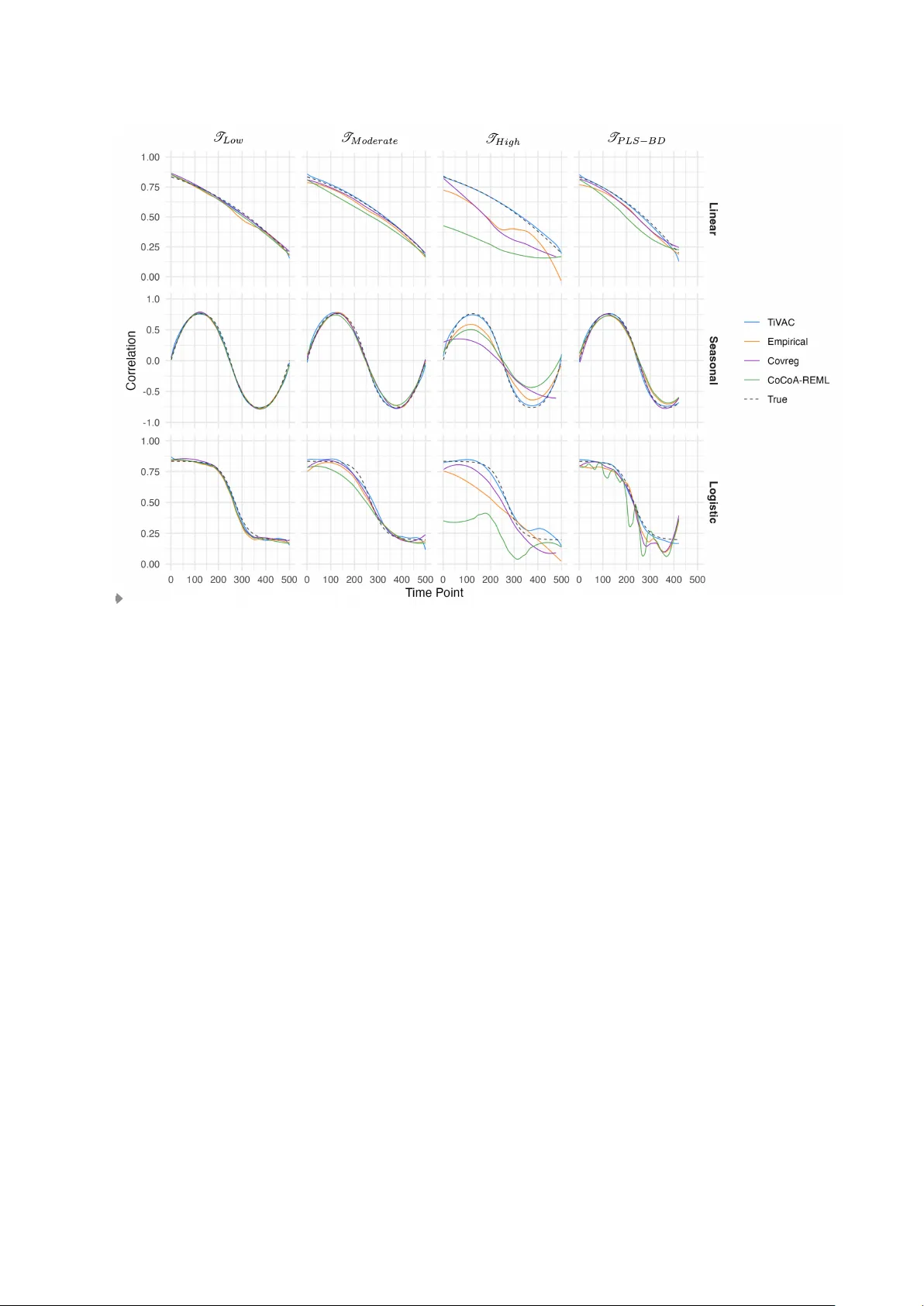
A Time-V arying and Co v ariate-Dep enden t Correlation Mo del for Multiv ariate Longitudinal Studies Qingzhi Liu 1 , Gen Li 1 , Anastasia K. Y o cum 2 , Melvin McInnis 2 , Brian D. A they 2 , 3 , V eerabhadran Baladandayuthapani 1 , ∗ 1 Departmen t of Biostatistics, Univ ersit y of Mic higan, Ann Arb or, Michigan, U.S.A. 2 Departmen t of Psychiatry , Universit y of Michigan, Ann Arb or, Mic higan, U.S.A. 3 Departmen t of Computational Medicine and Bioinformatics, Universit y of Michigan, Ann Arb or, Mic higan, U.S.A. * email: veerab@umic h.edu Summar y: In m ultiv ariate longitudinal studies, associations b etw een outcomes often exhibit time-v arying and individual lev el heterogeneit y , motiv ating the modeling of correlations as an explicit function of time and cov ariates. Ho wev er, most existing methods for correlation analysis fail to sim ultaneously capture the time-v arying and co v ariate- dep enden t effects. W e propose a Time-V arying and Cov ariate-Dep endent (TiV AC) correlation model that jointly allo ws cov ariate effects on correlation to change flexibly and smo othly across time. TiV AC emplo ys a biv ariate Gaussian mo del where the co v ariate-dependent correlations are mo deled semiparametrically using p enalized splines. W e dev elop a p enalized maxim um lik eliho od-based Newton–Raphson algorithm, and inference on time-v arying effects is provided through sim ultaneous confidence bands. Sim ulation studies show that TiV A C consistently outp erforms existing metho ds in accurately estimating correlations across a wide range of settings, including binary and con tin uous co v ariates, sparse to dense observ ation sc hedules, and across diverse correlation tra jectory patterns. W e apply TiV AC to a psychiatric case study of 291 bipolar I patients, mo deling the time-v arying correlation b et ween depression and anxiet y scores as a function of their clinical v ariables. Our analyses rev eal significant heterogeneity asso ciated with gender and nerv ous-system medication use, which v aries with age, revealing the complex dynamic relationship betw een depression and anxiety in bip olar disorders. Key words: co v ariate-dep endent correlation; dynamic correlation; functional data analysis; mo od dynamics; m ul- tiv ariate longitudinal data. TiV AC Corr elation 1 1. INTR ODUCTION Multiv ariate longitudinal data often reveal that asso ciations b et ween outcomes are neither constan t o v er time nor uniform across individuals. As an example, in psyc hiatric researc h, depression and anxiet y are commonly regarded as highly comorbid conditions(Kalin, 2020). In terestingly , in our application to bip olar I disorder (BP-I) patients, the concurrent corre- lation b etw een PHQ-9 (depression score; Kro enk e et al. (2001)) and GAD-7 (anxiet y score; Spitzer et al. (2006)) w as heterogeneous across patien ts, with some exhibiting very high correlations and others lo w or near zero (as sho wn in Figure 1A). T o further c haracterize this heterogeneit y , w e found that the correlation also v aried with patien t-sp ecific cov ariates such as age and an tipsyc hotic use frequency , as illustrated b y the three-dimensional correlation surface in Figure 1B. These findings underscore the imp ortance of accoun ting for b oth time-v arying and co v ariate-dep enden t heterogeneity in correlation, that could manifest in other con texts as well. This p oint is also highligh ted b y the ubiquitous Simpson’s paradox: subgroup-lev el correlations can v anish or even reverse relative to a fixed p opulation-level correlation (Blyth, 1972). This motiv ates the statistical question of mo deling correlations of outcomes ( ρ ) as an explicit function of time ( t ) and cov ariates ( X ), as ρ ( t, X ) in multiv ariate longitudinal studies. [Figure 1 ab out here.] In the con text of co v ariate-dep endent correlations (i.e. ρ ( X )), Bartlett (1993) first con- sidered correlation as a function of a discrete third v ariable. How ever, this metho d requires large subgroup-sp ecific sample sizes and is limited to a single discrete co v ariate (Dufera et al., 2023). Subsequent extensions hav e allo wed correlation to dep end on b oth con tin uous and discrete co v ariates within a biv ariate Gaussian framew ork, with parameters estimated via restricted maxim um lik eliho od (REML) (Wilding et al., 2011) and second-order generalized estimating equations (GEE2) (Ho et al., 2010). More recently , T u et al. (2022) introduced 2 the cov ariate-dependent pairwise correlation mo del with association size (CoCoA) and com- pared the p erformance of REML and GEE2 estimators with maximum lik eliho o d estimators (MLE). Another broad class of metho ds fo cuses on mo deling co v ariate-dep enden t cov ariance or correlation for more than t wo outcomes through parameterizations or transformations that ensure the cov ariance or correlation matrix remains positive definite (P ourahmadi, 1999; Chiu et al., 1996; Hoff and Niu, 2012; Ni et al., 2019; Archak ov and Hansen, 2021). Despite these adv ancements, the aforemen tioned mo dels do not explicitly address time- v arying correlations. Estimating cov ariate-dep enden t correlations separately at eac h time p oin t can substantially reduce statistical p o w er, particularly when data are irregularly ob- serv ed. Although one might consider treating time as a single co v ariate (Wilding et al., 2011; T u et al., 2022), this strategy often imp oses a linearity assumption on the time-v arying effects, whic h ma y obscure p otentially dynamic and nonlinear patterns in the correlation structure. F or instance, in our motiv ating application, W eb Figure 4 displays the mon thly P earson correlation b et w een depression and anxiet y severit y across different ages. When examining the full cohort or stratifying b y gender, the estimated correlation tra jectories rev eal significant noise that masks the underlying true dynamic pattern, thereby motiv ating the use of a flexible nonlinear mo deling approach. Although several statistical approac hes– including DCC-GAR CH (Engle, 2002), DSEM (Asparouho v et al., 2017), and idP A C (Kundu et al., 2021)–ha v e b een prop osed to capture time-v arying relationships among v ariables ( ρ ( t )), none directly or jointly mo del ho w co v ariates affect correlations o v er time and pro vide statistical inference on these time-v arying effects, i.e. ρ ( t, X ). T o this end, w e prop ose a Time-V arying and Co v ariate-Dep enden t (TiV A C) correlation mo del, which join tly mo dels time-v arying and co v ariate-dep enden t correlations. TiV A C fo- cuses on concurrent correlations b et w een pairs of outcomes ov er time and facilitates statistical inference on how co v ariate effects on correlation might c hange with time. Under a biv ariate TiV AC Corr elation 3 Gaussian mo del, we apply a Fisher transformation to the correlation parameter and formulate the transformed correlation as a linear function of cov ariates with co efficien ts that v ary o v er time. T o capture the dynamic nature of these co efficients, we emplo y functional data analysis metho ds using spline-based constructions, which offer tw o main b enefits: flexible mo deling of cov ariate and time effects, and b orrowing strength across adjacen t time p oints. F or estimation, we develop a computationally efficient strategy incorp orating p enalization to ensure spline smo othness and in terpretabilit y , and maximize the p enalized lik eliho od with a Newton–Raphson algorithm. T o test nonlinear time-v arying and co v ariate effects, we con- struct sim ultaneous confidence bands to con trol for m ultiple testing. In sim ulations, TiV A C consisten tly outp erforms several comp eting state-of-the-art approaches in estimating ρ ( t, X ) across v arious time-dep enden t correlation functions and cov ariate t yp es, under b oth correctly sp ecified and missp ecified mo dels. W e further applied TiV A C to mo o d tra jectory data from 291 BP-I patients enrolled in the Prech ter Longitudinal Study of Bip olar Disorder (PLS- BD) (McInnis et al., 2018; Y o cum et al., 2023), examining how patien t c haracteristics and clinical in terv en tions w ere asso ciated with the correlation b et w een PHQ-9 and GAD-7 scores across patien ts’ age. Our results revealed that the o v erall correlation b et w een depression and anxiet y increa sed sligh tly with age. Notably , males exhibited higher correlations than females at y ounger ages. Additionally , while higher usage of nerv ous system-related medications and an tipsyc hotics w as linked to lo wer correlations in early adultho o d, this relationship rev ersed at older ages; in con trast, mo o d stabilizer use w as consisten tly asso ciated with lo w er correlations. The remainder of the pap er is organized as follo ws. Section 2 details the TiV A C mo del form ulation. Sections 3.1 and 3.2 describe the spline represen tation and estimation pro cedure of co efficients, and Section 3.3 outlines the construction of simultaneous confidence bands for inference. Sim ulation results for correctly sp ecified data are presented in Section 4.1, 4 while Section 4.2 inv estigates mo del p erformance under incorrect sp ecifications. Section 5 demonstrates the application of TiV AC in the BP-I patien t mo od tra jectory study . Section 6 concludes with a discussion of our findings and future research directions. 2. TiV A C MODEL W e first outline the data structure and the TiV A C mo del framew ork. The observ ed data consist of t w o main comp onen ts: a pair of concurren t and irregular longitudinal outcomes and a set of p co v ariates. Sp ecifically , let n denote the num b er of individuals. F or each individual i , let Y i =  { Y i 1 ( t i 1 ) , Y i 2 ( t i 1 ) } , . . . , { Y i 1 ( t im i ) , Y i 2 ( t im i ) }  represen t the v ector of observ ed outcomes, where Y i 1 ( t ij ) and Y i 2 ( t ij ) are the first and second outcomes for individual i at time t ij , m i is the num b er of observ ation times for individual i , and t ij denotes the j -th observ ation time for individual i . Let Y = ( Y T 1 , . . . , Y T n ) represen t the collection of observ ed outcomes for all individuals. Additionally , let Y i ( t ij ) = { Y i 1 ( t ij ) , Y i 2 ( t ij ) } T represen t the biv ariate outcome pair for individual i at time t ij . The co v ariate information is represented by a design matrix X of dimensions n × p , where n > p (with p low-dimensional), and X i is the p -dimensional co v ariate vector for individual i . F or eac h individual i at given time t ij , we assume the concurrently observ ed outcomes follo w a biv ariate normal distribution with a co v ariate-dep enden t and time-v arying correlation:    Y i 1 ( t ij ) Y i 2 ( t ij )    ∼ N  0 , Σ ( t ij , X i )  , where Σ ( t ij , X i ) =    σ 2 1 ρ ( t ij , X i ) σ 1 σ 2 ρ ( t ij , X i ) σ 1 σ 2 σ 2 2    . (1) Here, ρ ( t ij , X i ) referred to as the TiV A C correlation, dep ends explicitly on b oth the obser- v ation time t ij and the cov ariate v ector X i . W e emphasize the dynamic nature of concurrent correlation by allowing ρ ( t ij , X i ) to v ary con tin uously ov er time. Since ρ is constrained within the interv al [ − 1 , 1], the Fisher transformation is emplo y ed to TiV AC Corr elation 5 map it onto the real line as, η ( t ij , X i ) = ln  1 + ρ ( t ij , X i ) 1 − ρ ( t ij , X i )  . The transformed correlation η ( t ij , X i ) is then mo deled via a v arying-co efficien t linear form as, η ( t ij , X i ) = X T i β ( t ij ) , (2) where β ( t ij ) is a co efficien t vector function of time. Of particular interest, the k -th element of β ( t ij ), denoted as β k ( t ij ), represents the time-v arying effect of the k -th co v ariate on the correlation. This sp ecification allo ws the concurrent correlation to depend jointly on time and co v ariates through interpretable and nonlinear co efficient tra jectories, and can be construed as a generalization of CoCoA mo del (T u et al., 2022). Building on the sp ecification ab ov e, we imp ose the following additional assumptions to ensure iden tifiabilit y and in terpretability of TiV AC mo del: (1) each outcome pair has zero mean, which can b e ac hiev ed, for example, through a flexible de-meaning approach such as the one prop osed by Patil et al. (2022); (2) the marginal v ariances are constant o v er time ( σ 2 1 , σ 2 2 ); since Co v { Y i 1 ( t ) , Y i 2 ( t ) } = ρ ( t, X i ) σ 1 ( t ) σ 2 ( t ), time-v arying marginal v ariances w ould confound marginal scale with dep endence, complicating inference on ρ ( t, X i ), esp e- cially under irregular designs (cf. Kundu et al. (2021)); and (3) there is no auto correlation across distinct time p oints, thereby fo cusing on dynamic heterogeneity in the concurren t correlation while balancing mo del complexit y and computational efficiency . 3. SPLINE CONSTR UCTION AND ESTIMA TION T o obtain a flexible and smo oth estimator ˆ β k ( t ), we represen t the co efficien t functions using B-splines (de Bo or, 2001), with kno wn basis functions and spline co efficien ts to b e estimated, as describ ed in Section 3.1. Because direct maximum-lik eliho od estimation of spline co efficien ts is sensitive to the n um b er and placement of knots, we incorp orate a 6 smo othing p enalt y on the spline co efficien ts, ensuring stabilit y while retaining the abilit y to capture significan t lo cal changes (Section 3.2). Finally , to address multiple comparisons arising from ev aluating co v ariate effects sim ultaneously across numerous time p oints, we dev elop a b o otstrap-based inference framework to construct simultaneous confidence bands, ensuring that the entire tra jectory of cov ariate effects lies within the bands with a sp ecified confidence level (Section 3.3). 3.1 Spline r epr esentation of nonline ar c ovariate effe cts Direct estimation of β ( t ij ) is not feasible, as it is infinite-dimensional. T o address this, we appro ximate it using a finite-dimensional B-spline representation (de Bo or, 2001). B-splines are piecewise p olynomial functions, with the order of the spline determining the degree of the p olynomial; a common choice is cubic B-splines (order 4). The num b er and placement of knots control the flexibilit y of the spline; more knots allo w for greater flexibility , while few er knots lead to smoother estimates. Sp ecifically , let b ( t ij ) denote a q -dimensional v ector of B- spline basis functions ev aluated at time t ij , where q dep ends on the num b er of knots and the spline order. F or the i -th individual, the B-spline basis functions ev aluated at all observ ed time p oin ts are organized in to a spline basis matrix, B i =  b ( t i 1 ) · · · b ( t im i )  ⊤ ∈ R m i × q . Inc orp or ating B-splines into TiV A C. F or each cov ariate k , the corresp onding time-v arying co efficien t β k ( t ij ) in β ( t ij ) can then b e expressed as: β k ( t ij ) = b ( t ij ) T θ k , (3) where θ k is a (lo w er) q -dimensional vector of spline co efficients. Substituting (3) into (2), the only parameters to estimate are the spline co efficients, θ k , for k = 1 , . . . , p . T o simplify the represen tation, w e com bine the spline bases and co v ariates into a single unified structure. Sp ecifically , for the i -th individual at time t ij , we define a new cov ariate vector A i,j = X T i ⊗ b ( t ij ) with length q · p , where ⊗ denotes the Kroneck er pro duct. Let θ = ( θ T 1 , θ T 2 , . . . , θ T p ) T , a vector of length q · p , represent all spline co efficien ts across the p co v ariates. The Fisher- TiV AC Corr elation 7 transformed correlation for individual i at time t ij can then b e expressed as: η ( t ij , X i ) = A T i,j θ . After θ is estimated, it can b e substituted in to Equation 3 to obtain the in terpretable co efficien t functions β k ( t ij ). 3.2 Spline c o efficient estimation Smo othness p enalty on spline c o efficients. T o estimate the spline co efficients θ , we maxi- mize a penalized log-likelihoo d function that incorp orates a smoothness p enalty on the B- spline co efficients. The p enalty term ensures stability in the estimation pro cess and preven ts o v erfitting. Rather than using the traditional integral of squared deriv ativ es, we adopt a difference p enalt y on adjacent spline co efficien ts, as prop osed by Eilers and Marx (1996). This discrete p enalt y simplifies computation while pro viding a close approximation to the smo othness measure achiev ed b y in tegral-based methods. Sp ecifically , w e emplo y the second- order difference p enalty , defined as: P ( θ k ) = 1 2 λ k θ T k D T 2 D 2 θ k , where D 2 represen ts the second-order difference op erator matrix, and λ k > 0 is the smo othing parameter. Sp ecifically , D 2 θ k yields a v ector whose j -th element is θ k,j − 2 θ k,j +1 + θ k,j +2 . Th us, this p enalt y encourages adjacen t spline co efficients to remain close, p enalizing curv ature and promoting smo othness in the estimated co efficien t functions. Higher-order difference p enalties can b e easily extended within this framew ork. As suggested by Eilers and Marx (1996), using a relatively large n um b er of knots is advisable. This strategy eliminates the need to balance low versus high num b ers of knots, which in unp enalized metho ds can yield drastically different smo othness levels. How ev er, we caution against using an excessiv ely dense grid of knots, as this can inflate the num b er of parameters and lead to insufficien t data b et ween adjacent knots, p oten tially complicating mo del fitting. Estimation of spline c o efficien ts. Incorp orating the smo othness p enalt y , the p enalized log- 8 lik eliho o d function for the spline co efficien ts is given b y: l penalized ( θ ; Y , A ) = log L ( θ ; Y , A ) − 1 2 p X k =1 λ k θ T k D T 2 D 2 θ k . (4) Here, log L ( θ ; Y , A ) represen ts the log-likelihoo d function for all individuals, incorp orating their m i biv ariate outcomes: log L ( θ ; Y , A ) = − 1 2 n X i =1 m i X j =1 { log(2 π ) + log | Σ ( t ij , X i ) | + Y i ( t ij ) T Σ ( t ij , X i ) − 1 Y i ( t ij ) } . T o estimate the spline co efficien ts θ , we maximize the p enalized log-likelihoo d function defined in (4) with resp ect to θ , given certain p enalized parameters λ k , k = 1 , . . . , p : ˆ θ = arg max θ l penalized ( θ ; Y , A ) . W e employ the Newton–Raphson algorithm to iterativ ely update θ . In addition, the smooth- ing parameters { λ k } p k =1 are optimized via cross-v alidation b y maximizing the held-out log- lik eliho o d l ( ˆ θ ; Y , A ). F urther algorithmic details are pro videdin W eb App endix A.1. Estimation of the TiV AC c orr elation. After obtaining the optimal smo othing parameters, the mo del is fit using all a v ailable samples to estimate the optimal ˆ θ . Let B b e the spline basis matrix ev aluated at all time p oin ts from 1 to max i,j ( t ij ), having dimensions max i,j ( t ij ) × q , where max i,j ( t ij ) denotes the maxim um observ ed time across all individuals. The estimated co efficien t tra jectory ˆ β k ( t ), for t = 1 , . . . , max i,j ( t ij ), is given b y ˆ β k ( t ) = B ˆ θ k , whic h measures the k -th cov ariate’s time-v arying effect on the correlation. The correlation tra jectory for co v ariate X i can then b e expressed as: ˆ ρ ( t, X i ) = tanh ( X k X ik ˆ β k ( t ) ) , where X ik is the k th co v ariate for individual i . 3.3 Simultane ous c onfidenc e b and estimation and infer enc e After estimating β k ( t ), it is imp ortant to conduct inference to determine whether the cov ari- ate effect on the correlation at certain time p oints is significant. Instead of using p oin t wise TiV AC Corr elation 9 confidence bands, which only guarantee confidence at individual time p oin ts, w e use sim ul- taneous confidence bands that ensure the entire tra jectory of a function lies within the band with a sp ecified confidence level. Mathematically , a 100(1 − α )% sim ultaneous confidence band satisfies: P { L ( t ) ⩽ β k ( t ) ⩽ U ( t ) , ∀ t ∈ T } ⩾ 1 − α for all t ∈ T . This approach is crucial for addressing multiple comparison issues and provides broader co v erage compared to p oin t wise confidence bands. W e construct sim ultaneous confidence bands for β k ( t ) using a b o otstrap pro cedure that resamples individuals (with replacement), preserving the observ ed time p oin ts within each individual. Sp ecifically , our pro cedure consists of t w o nested b o otstrap lo ops, eac h serving a distinct purp ose. The outer b o otstrap lo op quantifies the v ariabilit y of the estimator ˆ β k ( t ) b y rep eatedly drawing b o otstrap samples Y ( b ) ( b = 1 , . . . , B ) and re-estimating the spline co efficien ts, yielding b o otstrap estimates ˆ β ( b ) k ( t ). T o a v oid underestimating the v ariabilit y of the outer b o otstrap estimates, we use an inner bo otstrap lo op to provide robust estimates of their standard deviations. Specifically , in eac h outer iteration b , w e p erform M additional b o otstrap resamples Y ( b,m ) ( m = 1 , . . . , M ) from the outer sample Y ( b ) , computing inner-lo op estimates ˆ β ( b,m ) k ( t ). F rom these inner b o otstrap samples, w e compute the sample standard deviation ˜ s k,t for each outer iteration. Next, w e compute the t-statistic for each outer iteration b follo wing Rupp ert et al. (2010): T ( b ) k = max t     ˆ β ( b ) k ( t ) − ˆ β k ( t ) ˜ s k,t     . The critical v alue T crit k is then obtained as the empirical (1 − α )-quan tile of the collection of t-statistics { T ( b ) k } B b =1 . As noted b y Rupp ert et al. (2010), when the sample size is large, T crit k can b e approximated with high accuracy for simultaneous confidence band estimation. Finally , the simultaneous confidence band is constructed as: ˆ β k ( t ) ± T crit k · s k,t , where s k,t is the o verall b o otstrap standard deviation of ˆ β ( b ) k ( t ) across all outer b o otstrap iterations b = 1 , . . . , B . A detailed summary of the entire pro cedure is provided in W eb App endix A.2. 10 4. SIMULA TION STUDIES W e ev aluate the estimation accuracy of the TiV AC correlation under four generativ e mo dels, c haracterized b y whether the univ ariate co v ariate is binary or contin uous and whether the underlying correlation structure follo ws a deterministic function or is influenced by random noise. F or p enalty parameter selection, we emplo y 10-fold cross-v alidation to determine the optimal v alue. W e compare the TiV AC correlation to three alternativ e metho ds. The first is the “Em- pirical” correlation tra jectory , calculated by computing the Pearson correlation b et ween the t w o outcomes at each observed time p oin t within eac h cov ariate group. The resulting correlations are then smo othed ov er time using LOESS regression, with candidate span v alues ranging from 0.1 to 1 in increments of 0.1. The optimal span is selected via 5-fold cross-v alidation. The second metho d is co v ariance regression (Co vReg) (Hoff and Niu, 2012), where the co v ariate-dep enden t co v ariance matrix of the tw o outcomes is calculated at each time p oin t, transformed in to a correlation matrix, and subsequen tly smo othed using the same LOESS approac h as in the Empirical metho d. The third metho d is CoCoA (T u et al., 2022), implemen ted with three different estimation tec hniques: MLE, REML (Wilding et al., 2011), and GEE2 (Ho et al., 2010). The resulting estimates are also smo othed using the same LOESS approac h as in the Empirical metho d. F ollo wing the recommendation of T u et al. (2022) to use CoCoA-REML, w e fo cus primarily on its p erformance in the main text; results for CoCoA-MLE and CoCoA-GEE2 are provided in W eb App endix B. F or the sim ulation settings, w e fix the sample size at n = 300 and set max i,j ( t ij ) = 500. Eac h individual i has m i observ ed time p oin ts drawn under one of four conditions: (1) a fixed 40 time p oints ( T H ig h ); (2) a random num b er of time p oin ts b et w een 3 and 40 ( T M oder ate ), mimic king the observed PLS-BD data; (3) a random num b er of time p oints b et w een 3 and 10 ( T Low ); and (4) an alternative setting in whic h the n umber of individuals TiV AC Corr elation 11 and time points matches those of the observ ed PLS-BD data, with max i,j ( t ij ) = 421 (see Section 5), denoted T P LS − B D . The outcomes Y i 1 ( t ij ) and Y i 2 ( t ij ) follo w a biv ariate normal distribution (Equation 1) with v ariances σ 2 1 = 1 and σ 2 2 = 4. T o generate the time- and cov ariate-dependent correlation ρ ( t ij , X i ), w e apply the Fisher transformation in tw o separate data-generating mo dels: a deterministic mo del (correctly sp ecified case), η ( t ij , X i ) = β 0 ( t ij ) + β 1 ( t ij ) X i , and a noisy mo del (missp ecified case), η ( t ij , X i ) = β 0 ( t ij ) + β 1 ( t ij ) X i + ϵ ( t ij ) , where ϵ ( t ij ) ∼ N  0 , σ noise  , and σ noise ∈ { 0 . 1 , 0 . 2 , 0 . 3 , 0 . 4 , 0 . 5 } . The four simulation scenarios considered in Sections 4.1 and 4.2 are: • Scenario 1: deterministic mo del with a binary co v ariate X i ∈ { 0 , 1 } ; • Scenario 2: deterministic mo del with a con tin uous cov ariate X i ∈ [0 , 1]; • Scenario 3: noisy mo del with a binary co v ariate X i ∈ { 0 , 1 } ; • Scenario 4: noisy mo del with a con tin uous cov ariate X i ∈ [0 , 1]. The co efficient functions β k ( t ) ( k = 0 , 1) are generated using one of three tra jectory patterns: linear, seasonal, or logistic. The true correlation curves, tanh { β 0 ( t ) + β 1 ( t ) } , are sho wn as dashed lines in Figure 2. F or mo del ev aluation, we compute the ro ot mean squared error (RMSE) by comparing eac h metho d’s estimated correlation to the true correlation curve o v er 50 replications. In the binary co v ariate scenario, RMSE is av eraged across time p oin ts for eac h cov ariate v alue (0 or 1), reflecting the deviation from the true correlation tra jectory in each group. In the con tin uous co v ariate scenario, RMSE is computed b y av eraging ov er b oth time p oin ts and a grid of 100 co v ariate v alues ranging from 0 to 1. 12 4.1 Simulations with deterministic c orr elation functions In Scenario 1, the underlying correlation function is deterministic, and the co v ariate is binary ( X = 0 for half the sample and X = 1 for the other half ). Panel A of T able 1 presen ts the RMSE and standard deviations (SD) results for TiV A C, Empirical, Co vReg, and CoCoA- REML across differen t co efficient function t yp es and time-p oin t settings. Ov erall, TiV AC ac hiev es the highest estimation accuracy under all settings, with its adv antage b ecoming more pronounced when few er time p oin ts are observed. Under T H ig h , the RMSE differences b et w een TiV A C and the other metho ds are mo dest (up to 0.02). By con trast, in the T Low setting, Empirical, CovReg, and CoCoA-REML exceed TiV A C’s RMSE by more than 0.1 in most cases. TiV AC also exhibits smaller SD than the comp eting metho ds, reflecting its stabilit y . TiV A C’s outp erformance could stem from its capacit y to borrow correlation infor- mation across time p oin ts via p enalized splines. Under the T Low setting, CovReg p erforms w orse than Empirical, and CoCoA-REML exhibits even p o orer p erformance. W e susp ect that CovReg and CoCoA-REML, as mo del-based approac hes, are particularly sensitive to data sparsit y . In practice, when only a few observ ations are a v ailable at certain time p oin ts, the iterativ e optimization in mo del-based metho ds may fail to con verge, leading to missing estimates of correlation. [T able 1 ab out here.] Figure 2 compares the estimated correlation curves from the four metho ds to the true curv e when X = 1 in Scenario 1. Each subplot corresp onds to a representativ e example from the first of 50 simulation runs (using a fixed random seed). The figure reveals tw o additional insigh ts. First, TiV A C b etter captures the tail b ehavior of the true correlation. F or instance, under the T P LS − B D logistic tra jectory , Empirical, Co vReg, and CoCoA-REML exhibit an up w ard trend on the righ t tail, whereas the true curve and TiV AC flatten out. Second, TiV AC’s spline-based p enalt y preserves a level of smo othness that aligns closely with the TiV AC Corr elation 13 true tra jectory , while p oin t wise-based estimates can b ecome ov erly smo othed (e.g., under the T Low seasonal tra jectory) or fluctuate sharply (e.g., CoCoA-REML under the T P LS − B D logistic tra jectory). One reason is that the large v ariabilit y of the p oint wise estimates b efore smo othing makes it difficult for LOESS regression to recov er the underlying correlation’s true smo othness. [Figure 2 ab out here.] F urthermore, W eb T able 1 presen ts sim ulation results for CoCoA-MLE, CoCoA-REML, and CoCoA-GEE2 in Scenario 1. Under the T Low setting, CoCoA-GEE2 outp erforms the other t w o estimators, while in other settings their p erformances are similar. Nevertheless, under the T Low setting, its p erformance remains inferior to that of TiV A C, Empirical, and Co vReg. In Scenario 2, we adopt the same ov erall simulation design as in Scenario 1 but treat the co v ariate as contin uous, ranging from 0 to 1. Unlike in Scenario 1, we fix each individual’s n um b er of observ ed time p oints at 10 to prev en t Co vReg from failing to con v erge under the T Low setting. Because Empirical cannot accommo date contin uous co v ariates, w e fo cus on TiV AC, CovReg, and CoCoA-REML. P anel B of T able 1 summarizes the RMSE results across differen t co efficien t function types and time-p oin t settings. TiV A C consisten tly outperforms Co vReg and CoCoA-REML. Moreov er, TiV AC exhibits similar p erformance in b oth Scenario 1 and Scenario 2 when the other settings are comparable, underscoring its robust p erformance for differen t co v ariate t yp es. CoCoA-REML consisten tly outperforms CovReg, likely because its parametric assumption at eac h time p oint aligns with how the data are generated in our sim ulation, leading to more stable estimates than Co vReg in this more complex scenario. [Figure 3 ab out here.] Figure 3 shows representativ e examples from the first run of eac h case (using a fixed random seed) under the T M oder ate setting in Scenario 2. The correlation heatmaps illustrate 14 ho w correlation v alues (in rainbow colors) depend on b oth time p oin ts (x-axis) and cov ariate v alues (y-axis). They rev eal that TiV A C’s estimated heatmap is not only m uc h closer to the true pattern but also displays smo other transitions across time and co v ariates. Additional comparisons of correlation heatmaps under the T Low , T H ig h , and T P LS − B D settings app ear in W eb Figures 1-3, resp ectively . Although CovReg and CoCoA-REML ha ve similar RMSE under T M oder ate and T P LS − B D , their heatmaps indicate that these t wo metho ds reco v er the true patterns in T P LS − B D more p o orly than they do in T M oder ate , illustrating ho w the irregular nature of the PLS-BD data complicates in terpretabilit y of Co vReg and CoCoA- REML. Finally , W eb T able 2 presen ts simulation results comparing CoCoA-MLE, CoCoA- REML, and CoCoA-GEE2 in Scenario 2. Unlik e Scenario 1, here CoCoA-REML p erforms b etter than CoCoA-GEE2 and is comparable to CoCoA-MLE. 4.2 Imp act of noise in c orr elation functions In b oth Scenario 3 (binary co v ariate) and Scenario 4 (con tinuous co v ariate), we in tro duce additional randomness in to the latent correlation function by letting σ noise v ary from 0.1 to 0.5. W e use the T M oder ate setting and compute the RMSE as in their resp ective baseline scenarios (i.e., with no random noise in the co efficien t function). As summarized in W eb T able 3 (for Scenario 3) and W eb T able 4 (for Scenario 4), all methods degrade in p erfor- mance as σ noise increases, but TiV A C consisten tly outp erforms the alternativ es and remains robust, main taining an av erage RMSE b elow 0.1. This robustness likely stems from TiV A C’s spline-based smo othing, whic h helps mitigate noise-induced fluctuations in the correlation estimates. W eb T able 5 (for Scenario 3) and W eb T able 6 (for Scenario 4) compare CoCoA-MLE, CoCoA-REML, and CoCoA-GEE2. In Scenario 3, CoCoA-GEE2 slightly outp erforms the other CoCoA estimators for linear and logistic co efficien t functions. In Scenario 4, CoCoA- MLE slightly p erforms b etter than CoCoA-REML, whic h in turn outp erforms CoCoA-GEE2, TiV AC Corr elation 15 for linear and logistic functions; whereas CoCoA-REML sligh tly outp erforms for the seasonal functions. 5. APPLICA TION TO MOOD TRAJECTORIES IN BIPOLAR P A TIENTS W e analyzed data from patients with BP-I enrolled in PLS-BD (McInnis et al., 2018; Y o cum et al., 2023), fo cusing on the PHQ-9 (Kro enke et al., 2001), a measure of depression severit y , and the GAD-7 (Spitzer et al., 2006), a measure of anxiety severit y , as mo o d outcomes. P atien ts’ substance use disorder status and medication use were incorporated as co v ariates. Depression and anxiety are highly prev alent and comorbid symptoms among individuals with bip olar disorder (Kalin, 2020). Ho wev er, our empirical analysis (Figure 1A) indicated heterogeneit y in their asso ciation o ver time. This pattern motiv ated use of the TiV A C mo del to characterize the dynamic correlation b etw een depression and anxiety and to ev aluate ho w patien t c haracteristics and clinical factors modulate this relationship. A b etter understanding of these patterns could elucidate disease mechanisms and inform p ersonalized treatment strategies (Kim et al., 2024). Mo o d outcomes w ere collected bimon thly , and medication use records w ere updated y early , with substantial b etw een-patien t v ariability in enrollmen t (baseline) dates and subsequent observ ation schedules. T o ensure a consisten t and interpretable timeline, w e used each patien t’s measured age as the time v ariable ( t ij ) in the TiV A C mo del. The dataset w as prepro cessed (Liu et al. 2025), follow ed by additional cleaning based on the following in- clusion criteria: (1) for each patien t, every observed time p oint m ust include b oth PHQ-9 and GAD-7 scores, and (2) the observ ed time p oin ts must corresp ond to ages b et w een 30 and 65. PHQ-9 and GAD-7 scores w ere then cen tered separately for males and females and subsequen tly transformed using a quantile transformation (T u et al., 2022) to approximate a Gaussian distribution. These prepro cessing steps ensured that the assumptions of the TiV AC mo del were fairly met. As shown in W eb T able 7, the dataset used for mo deling included 16 291 BP-I patien ts. Of these, 70.8% w ere female, 47.4% had a history of alcohol use disorder, and 28.9% had cannabis use disorder. Alcohol use disorder and cannabis use disorder status w ere assessed at enrollmen t and treated as time-in v ariant cov ariates. Medication-related co v ariates w ere defined based on (Liu et al. 2025) as follows: the av erage nerv ous system- related medications (whic h include all psyc hiatric medications) for each patient represen ted the mean coun t of those medications across observ ed time p oin ts, while the use frequency of eac h psyc hiatric medication reflected the prop ortion of observ ed time p oin ts where the medication w as tak en. These cov ariates w ere contin uous, with this summarization approac h necessitated by limitations in the medication data collection pro cess. W e applied the TiV A C mo del to each cov ariate separately to measure its av erage effect on the correlation b et ween PHQ-9 and GAD-7 scores o v er age in BP-I patien ts. Although the mo del can in principle handle m ultiple cov ariates, eac h cov ariate in tro duced a set of spline parameters. Because our data were highly irregular (e.g., few observ ations at certain time p oin ts), in tro ducing too man y parameters can lea d to unstable and unreliable estimates. Age w as recorded in mon ths for mo deling while visualized in years, with selected knots placed at interv als of 24 months. Without considering cov ariates, W eb Figure 5 sho ws that the correlation b et w een PHQ-9 and GAD-7 scores sligh tly increases with age, consistent with the literature (Lenze, 2003) suggesting higher comorbidit y b etw een PHQ-9 and GAD-7 in older individuals. Figure 4 presents the co efficient functions β 1 ( t ) in blue, representing the effect of each co v ariate on the correlation as age increases. The 95% sim ultaneous confidence bands (sho wn in gra y) indicate the p erio ds where the co v ariate effect w as significan t; sp ecifically , when the bands did not o v erlap with the zero co efficien t v alue (dashed line). F or gender, males exhibited significantly higher correlations than females as age increases, though this difference diminished gradually . F or the a v erage nervous system-related medications, increased usage TiV AC Corr elation 17 w as asso ciated with significan tly low er correlations until around age 50. Regarding an tipsy- c hotic use frequency , greater usage was asso ciated with lo w er correlations b efore age 50 and higher correlations after age 50, with the effects b eing significant at the endp oints of the observ ed range. F or mo o d stabilizer use frequency , higher usage was significantly asso ciated with low er correlations b etw een ages 40 and 55. Although the estimated co efficien t functions for these co v ariates app eared roughly linear in time, their significance could still v ary across the age range; b y con trast, assuming a time-in v ariant effect w ould imply the significance remains constant. In addition, the effect of antidepressan t use frequency exhibited a nonlinear pattern, as shown in its subplot, but there w as insufficient evidence to conclude a significant influence o v er time. Similarly , there w as no strong evidence of significant effects for alcohol use disorder or cannabis use disorder. Lastly , the relatively wider confidence bands at the tiles were likely due to less frequen t observ ations in those p erio ds. [Figure 4 ab out here.] T o further in terpret the TiV AC results, w e visualized the TiV A C correlations for the four co v ariates that exhibited significant effects during certain time p erio ds (Figure 5). Almost all TiV AC correlations across the four subplots exceeded 0.5, with exceptions observed when the av erage nerv ous system-related medication usage w as near 4 or the antipsyc hotic use frequency w as near 1, particularly around ages 30–35, as indicated in blue. The consisten tly high TiV AC correlations are consistent with the well-documented comorbidit y b etw een anx- iet y and depressive disorders (Kalin, 2020). Genetically , these disorders share a substantial lev el of risk factors (Hettema, 2008). At the neural circuit level, b oth inv olv e alterations in prefron tal-lim bic path w a ys that are critical for mediating emotional regulation pro cesses (Kalin, 2020). In addition, the TiV A C correlation for males on a verage was appro ximately 0.1 higher than that for females at age 30 but gradually diminished as age increases. Previous studies ha ve 18 sho wn that, in general, w omen with depression often exhibit greater comorbidity with anxiet y disorders than men, lik ely due to sex differences in neural circuits and molecular mechanisms related to anxiety and depression (Bangasser and Cuaren ta, 2021; Kornstein et al., 2000). Ho w ever, this area remains underexplored. Interestingly , within this BP-I cohort, w e observed the opp osite pattern, underscoring the need for further researc h in to sex-specific mec hanisms underlying mo o d and anxiety comorbidities in BP-I. F or nerv ous system-related medications, increased usage was asso ciated with lo w er corre- lations b efore age 40 (indicated by a shift from orange to blue) but with higher correlations b et w een ages 60 and 65 (indicated by a shift from green to orange). A similar, though not iden tical, age-dep endent pattern w as observed for antipsyc hotic use frequency , indirectly reflecting differences in drug responses across age groups. One p ossible explanation in v olves the brain’s neuroplasticity , which remains relatively high at younger ages (Park and Bischof, 2013), allo wing for greater adaptabilit y . In this context, nervous system-related medications ma y disrupt natural emotional regulation circuits, thereby w eakening correlations b et w een anxiet y and depressive symptoms. In con trast, higher mo o d stabilizer use frequency was asso ciated with slightly low er cor- relations (shifting from yello w to green) across all ages. Mo o d stabilizers are though t to mo dulate prefrontal-lim bic circuits inv olved in mo o d regulation (Schloesser et al., 2012). This stabilizing effect ma y slightly decouple the neural pro cesses underlying anxiet y and depression. [Figure 5 ab out here.] Ov erall, b y applying our TiV A C mo del to the mo o d data of BP-I patients, we rev ealed that the relationship betw een anxiet y and depression dep ends on gender, medication use, and age, highlighting the complexit y of moo d dynamics in BP-I patien ts. While these findings pro vide data-driven evidence, further v alidation is necessary to confirm these observ ations. TiV AC Corr elation 19 6. DISCUSSION In this work, we dev elop the Time-V arying and Co v ariate-Dep enden t (TiV A C) correlation mo del, which jointly mo dels time-v arying and cov ariate-dep enden t correlations. TiV A C ac- commo dates flexible, time-v arying cov ariate effects and time-resolv ed inference b y mo del- ing latent correlation regression co efficients as smo oth functions of time. In addition, our b o otstrap-based pro cedure for estimating simultaneous confidence bands mitigates concerns of m ultiple testing across time p oin ts. Sim ulation studies demonstrate that TiV AC consis- ten tly outp erforms comp eting metho ds in terms of correlation estimation accuracy across v arious settings. In our application to longitudinal mo od data from BP-I patien ts, TiV AC iden tified substantial heterogeneit y in the asso ciation b et ween depression and anxiety across age and patien t characteristics. These findings reflect v ariation in the correlation structure rather than changes in symptom severit y or treatmen t resp onse. This pap er primarily fo cuses on inference for the TiV AC correlation structure, and an in teresting future direction is to jointly mo del a flexible mean structure together with the TiV AC correlation structure. Curren tly , TiV AC assumes zero auto correlation within each outcome across different time p oints. Extending the biv ariate Gaussian framew ork to a m ultiv ariate or Gaussian-pro cess setting would allo w for correlations across time-p oints, but necessitates deep er in vestigation of the mo del-building and estimation pro cesses due to increased complexity and computational demands. Another promising direction is to accommo date non-Gaussian outcomes, giv en that many real-w orld datasets may exhibit sk ewness, zero-inflation, or discrete distributions. In this setting, copula-based metho ds ma y offer a flexible approac h to effectiv ely address these distributional challenges. Finally , although the curren t framew ork fo cuses on tw o correlated v ariables, extending TiV AC to higher-dimensional outcomes is a promising av en ue for future researc h; such extensions will require parameterizations that guaran tee p ositiv e definiteness of the correlation matrix. 20 When applying TiV A C in practice, sev eral considerations are imp ortan t for interpreting the results. The framework do es not allow for clear temporal separation b et w een exp osure and correlation; therefore, it estimates statistical asso ciations rather than predictiv e or causal effects. Moreo v er, the magnitude of correlation alone do es not directly translate to illness sev erit y , treatmen t resp onse, or prognosis. A CKNOWLEDGMENTS The authors thank the Heinz C. Prec h ter Bipolar Researc h Program for providing the data. The authors also thank Dr. Da vid Belmon te and Dr. Jie Sun for providing v aluable clinical p ersp ectiv es on the interpretation of the application results. FUNDING V eerabhadran Baladandayuthapani’s w ork w as supp orted by the National Institutes of Health gran ts R01CA244845-01A1 and P30 CA46592 and funds from the Universit y of Michigan Rogel Cancer Center and Sc ho ol of Public Health. D A T A A V AILABILITY The data used in this study w ere obtained under license from the Heinz C. Prec h ter Bip olar Researc h Program and are therefore not publicly a v ailable. Data are ho wev er a v ailable from the authors up on reasonable request and with permission from the Heinz C. Prec hter Bip olar Researc h Program. The co de and R pack age used to repro duce all results presented in this pap er are av ailable at h ttps://github.com/ba yesrx/TiV A C. TiV AC Corr elation 21 References Arc hak ov, I. and Hansen, P . R. (2021). A new parametrization of correlation matrices. Ec onometric a 89, 1699–1715. Asparouho v, T., Hamak er, E. L., and Muth ´ en, B. (2017). Dynamic structural equation mo dels. Structur al Equation Mo deling: A Multidisciplinary Journal 25, 359–388. Bangasser, D. A. and Cuaren ta, A. (2021). Sex differences in anxiety and depression: Circuits and mechanisms. Natur e R eviews Neur oscienc e 22, 674–684. Bartlett, R. F. (1993). Linear mo delling of p earson’s pro duct momen t correlation co efficien t: An application of fisher’s z-transformation. The Statistician 42, 45. Blyth, C. R. (1972). On simpson’s paradox and the sure-thing principle. Journal of the A meric an Statistic al Asso ciation 67, 364. Chiu, T. Y., Leonard, T., and Tsui, K.-W. (1996). The matrix-logarithmic cov ariance model. Journal of the Americ an Statistic al Asso ciation 91, 198. de Bo or, C. (2001). A pr actic al guide to splines . Springer. Dufera, A. G., Liu, T., and Xu, J. (2023). Regression mo dels of p earson correlation co efficien t. Statistic al The ory and R elate d Fields 7, 97–106. Eilers, P . H. and Marx, B. D. (1996). Flexible smo othing with b-splines and p enalties. Statistic al Scienc e 11, . Engle, R. (2002). Dynamic conditional correlation. Journal of Business & Ec onomic Statistics 20, 339–350. Hettema, J. M. (2008). What is the genetic relationship b et w een anxiety and depression? A meric an Journal of Me dic al Genetics Part C: Seminars in Me dic al Genetics 148C, 140–146. Ho, Y.-Y., P armigiani, G., Louis, T. A., and Cope, L. M. (2010). Mo deling liquid asso ciation. Biometrics 67, 133–141. 22 Hoff, P . D. and Niu, X. (2012). A cov ariance regression mo del. Statistic a Sinic a 22, . Kalin, N. H. (2020). The critical relationship betw een anxiet y and depression. A meric an Journal of Psychiatry 177, 365–367. Kim, H., McInnis, M. G., and Sp erry , S. H. (2024). Longitudinal dynamics b et w een anxiet y and depression in bip olar sp ectrum disorders. Journal of Psychop atholo gy and Clinic al Scienc e 133, 129–139. Kornstein, S., Schatzberg, A., Thase, M., Y onkers, K., McCullough, J., Keitner, G., Gelen- b erg, A., Ryan, C., Hess, A., Harrison, W., and et al. (2000). Gender differences in c hronic ma jor and double depression. Journal of Affe ctive Disor ders 60, 1–11. Kro enk e, K., Spitzer, R. L., and Williams, J. B. (2001). The phq-9: v alidity of a brief depression severit y measure. Journal of Gener al Internal Me dicine 16, 606–613. Kundu, S., Ming, J., No cera, J., and McGregor, K. M. (2021). Integrativ e learning for p opulation of dynamic netw orks with cov ariates. Neur oImage 236, 118181. Lenze, E. J. (2003). Comorbidity of depression and anxiety in the elderly . Curr ent Psychiatry R ep orts 5, 62–67. McInnis, M. G., Assari, S., Kamali, M., Ryan, K., Langenec k er, S. A., Saunders, E. F., V ersha, K., Ev ans, S., O’Shea, K. S., Mow er Prov ost, E., et al. (2018). Cohort profile: the heinz c. prec h ter longitudinal study of bip olar disorder. International journal of epidemiolo gy 47, 28–28n. Ni, Y., Stingo, F. C., and Baladanda yuthapani, V. (2019). Ba y esian graphical regression. Journal of the Americ an Statistic al Asso ciation 114, 184–197. P ark, D. C. and Bischof, G. N. (2013). The aging mind: Neuroplasticit y in resp onse to cognitiv e training. Dialo gues in Clinic al Neur oscienc e 15, 109–119. P atil, I., Mako wski, D., Ben-Shac har, M. S., Wiernik, B. M., Bacher, E., and L ¨ udeck e, D. (2022). Datawizard: An r pac k age for easy data preparation and statistical transforma- TiV AC Corr elation 23 tions. Journal of Op en Sour c e Softwar e 7, 4684. P ourahmadi, M. (1999). Join t mean-cov ariance mo dels with applications to longitudinal data: Unconstrained parameterisation. Biometrika 86, 677–690. Rupp ert, D., W and, M. P ., and Carroll, R. J. (2010). Semip ar ametric r e gr ession . Cambridge Univ ersit y Press. Sc hlo esser, R. J., Martino wic h, K., and Manji, H. K. (2012). Moo d-stabilizing drugs: Mec hanisms of action. T r ends in Neur oscienc es 35, 36–46. Spitzer, R. L., Kro enk e, K., Williams, J. B., and L¨ ow e, B. (2006). A brief measure for assessing generalized anxiety disorder. A r chives of Internal Me dicine 166, 1092. T u, D., Mahon y , B., Mo ore, T. M., Bertolero, M. A., Alexander-Blo c h, A. F., Gur, R., Bassett, D. S., Satterthw aite, T. D., Raznahan, A., and Shinohara, R. T. (2022). Co coa: Conditional correlation mo dels with asso ciation size. Biostatistics 25, 154–170. Wilding, G. E., Cai, X., Hutson, A., and Y u, Z. (2011). A linear mo del-based test for the heterogeneit y of conditional correlations. Journal of Applie d Statistics 38, 2355–2366. Y o cum, A. K., Anderau, S., Bertram, H., Burgess, H. J., Co c hran, A. L., Deldin, P . J., Ev ans, S. J., Han, P ., Jenkins, P . M., Kaur, R., and et al. (2023). Cohort profile up date: The heinz c. prec h ter longitudinal study of bip olar disorder. International Journal of Epidemiolo gy 52, . 24 Figure 1. PHQ-9 and GAD-7 tra jectories and correlation heterogeneit y . (A) Irregular longitudinal tra jectories of PHQ-9 (depression; blue) and GAD-7 (anxiety; red) for tw o representativ e BP-I patients. The concurren t, within-patient P earson correlation is high for the top patien t ( ρ = 0 . 88) and low for the b ottom patien t ( ρ = − 0 . 15). (B) Three- dimensional correlation surface sho wing ho w the PHQ–GAD correlation (z-axis) v aries with age (x-axis) and an tipsychotic-use frequency (y-axis). Color enco des the correlation v alue through rainbow scale. TiV AC Corr elation 25 Figure 2. Represen tative curv e estimations in Scenario 1. Comparison b et ween the estimated correlation curves from four metho ds (TiV A C, Empirical, Co vReg and CoCoA- REML) and the true correlation curve when co v ariate X = 1. The figure presen ts nine indep enden t cases, representing three t yp es of co efficien t functions and three settings for the n um b er of time p oin ts p er individual. Each case sho ws a represen tative example from the first run of the sim ulation out of 50 replications (using a fixed random seed for all cases). The TiV AC, Empirical, CovReg and CoCoA-REML metho ds are depicted as blue, orange, purple and green curv es, resp ectiv ely , while the true tra jectory is represented by a dashed blac k curve. 26 Figure 3. Represen tativ e heatmap estimations under T M oder ate setting in Sce- nario 2. Comparison b etw een the estimated correlation heatmaps from three metho ds (TiV AC, Co vReg and CoCoA-REML) and the true correlation heatmap under T M oder ate setting. In each heatmap, correlation v alues are color-co ded, with red indicating higher correlations and blue indicating low er correlations. Each heatmap displa ys correlation patterns o v er time for differen t v alues of the con tin uous co v ariate. The figure presen ts three indep enden t cases, eac h represen ting one of the three t ypes of coefficient functions. Eac h case sho ws a represen tativ e example from the first run of the sim ulation (using a fixed random seed for all cases). TiV AC Corr elation 27 Figure 4. Results of TiV A C co efficient functions on PLS-BD data. TiV AC co efficien t functions ov er age for seven co v ariates, measuring their effects on the correlation b et w een PHQ-9 and GAD-7 in PLS-BD. F or eac h co v ariate, the co efficient function β ( t ) is sho wn in blue, with a gra y band representing the 95% simultaneous confidence band. The dashed black line at zero indicates no effect. 28 Figure 5. Results of TiV AC correlations on PLS-BD data. Visualization of TiV A C correlations b et ween PHQ-9 and GAD-7 for four cov ariates with significant or near-significan t age p erio ds. F or gender (top-left subplot), the TiV A C correlation curv e o v er age is shown in red for females and blue for males. F or the other three heatmaps, the corresp onding co v ariates are con tinuous, with the cov ariate v alues on the y-axis, age on the x-axis, and heatmap colors representing the TiV AC correlation v alues. TiV AC Corr elation 29 T able 1 Simulation r esults for Sc enarios 1 and 2. Simulation r esults c omp aring the p erformance of TiV A C and c omp eting metho ds under differ ent c o efficient function typ es and numb e r of observe d time p oints p er individual. Panel A (Sc enario 1) pr esents r o ot me an squar e d err or (RMSE) with standar d deviation (SD) in p ar entheses when the c ovariate is binary; the time-varying c orr elation is ρ 0 ( t ) when X = 0 and ρ 1 ( t ) when X = 1 . Panel B (Sc enario 2) pr esents RMSE (SD) when the c ovariate is c ontinuous. P anel A: Scenario 1 (binary cov ariate) Co efficien t # of Time Correlation RMSE (SD) F unctions Poin ts F unctions TiV AC Empirical Co vReg CoCoA-REML Linear T Low ρ 0 ( t ) 0.02 (0.01) 0.16 (0.04) 0.20 (0.10) 0.36 (0.03) ρ 1 ( t ) 0.02 (0.01) 0.15 (0.04) 0.20 (0.09) 0.34 (0.04) T M oderate ρ 0 ( t ) 0.01 (0.01) 0.06 (0.02) 0.04 (0.01) 0.06 (0.02) ρ 1 ( t ) 0.01 (0.01) 0.06 (0.02) 0.04 (0.02) 0.07 (0.02) T H ig h ρ 0 ( t ) 0.01 (0.01) 0.03 (0.01) 0.02 (0.01) 0.03 (0.01) ρ 1 ( t ) 0.01 (0.01) 0.03 (0.01) 0.02 (0.01) 0.02 (0.01) T P LS − B D ρ 0 ( t ) 0.01 (0.01) 0.04 (0.02) 0.04 (0.02) 0.09 (0.02) ρ 1 ( t ) 0.02 (0.01) 0.06 (0.02) 0.05 (0.02) 0.10 (0.02) Seasonal T Low ρ 0 ( t ) 0.06 (0.02) 0.12 (0.04) 0.17 (0.07) 0.08 (0.03) ρ 1 ( t ) 0.06 (0.02) 0.16 (0.03) 0.19 (0.06) 0.22 (0.03) T M oderate ρ 0 ( t ) 0.04 (0.01) 0.06 (0.02) 0.07 (0.02) 0.05 (0.02) ρ 1 ( t ) 0.03 (0.01) 0.07 (0.02) 0.07 (0.02) 0.07 (0.01) T H ig h ρ 0 ( t ) 0.03 (0.01) 0.04 (0.01) 0.04 (0.01) 0.04 (0.01) ρ 1 ( t ) 0.03 (0.01) 0.04 (0.01) 0.04 (0.01) 0.04 (0.01) T P LS − B D ρ 0 ( t ) 0.03 (0.01) 0.05 (0.02) 0.07 (0.02) 0.05 (0.02) ρ 1 ( t ) 0.03 (0.01) 0.08 (0.02) 0.08 (0.02) 0.08 (0.02) Logistic T Low ρ 0 ( t ) 0.05 (0.02) 0.14 (0.04) 0.19 (0.06) 0.36 (0.04) ρ 1 ( t ) 0.05 (0.02) 0.16 (0.05) 0.22 (0.08) 0.34 (0.04) T M oderate ρ 0 ( t ) 0.03 (0.01) 0.06 (0.01) 0.05 (0.01) 0.07 (0.02) ρ 1 ( t ) 0.03 (0.01) 0.06 (0.01) 0.05 (0.01) 0.07 (0.02) T H ig h ρ 0 ( t ) 0.02 (0.01) 0.03 (0.01) 0.03 (0.01) 0.03 (0.01) ρ 1 ( t ) 0.02 (0.01) 0.03 (0.01) 0.03 (0.01) 0.03 (0.01) T P LS − B D ρ 0 ( t ) 0.03 (0.01) 0.05 (0.01) 0.04 (0.02) 0.10 (0.02) ρ 1 ( t ) 0.03 (0.01) 0.06 (0.02) 0.06 (0.02) 0.09 (0.02) P anel B: Scenario 2 (con tinuous cov ariate) Co efficien t # of Time RMSE (SD) F unctions Poin ts TiV AC Co vReg CoCoA-REML Linear T Low 0.03 (0.01) 0.21 (0.04) 0.15 (0.02) T M oderate 0.02 (0.01) 0.08 (0.01) 0.06 (0.01) T H ig h 0.01 ( < 0.01) 0.05 (0.01) 0.03 (0.01) T P LS − B D 0.02 (0.01) 0.10 (0.01) 0.09 (0.01) Seasonal T Low 0.04 (0.01) 0.21 (0.05) 0.12 (0.02) T M oderate 0.03 (0.01) 0.09 (0.01) 0.07 (0.01) T H ig h 0.03 ( < 0.01) 0.05 (0.01) 0.04 (0.01) T P LS − B D 0.03 (0.01) 0.09 (0.01) 0.07 (0.01) Logistic T Low 0.05 (0.01) 0.21 (0.04) 0.16 (0.02) T M oderate 0.03 (0.01) 0.09 (0.01) 0.06 (0.01) T H ig h 0.02 ( < 0.01) 0.05 (0.01) 0.03 (0.01) T P LS − B D 0.03 (0.01) 0.09 (0.02) 0.09 (0.01)