Adjacency Spectral Embeddings of Correlation Networks

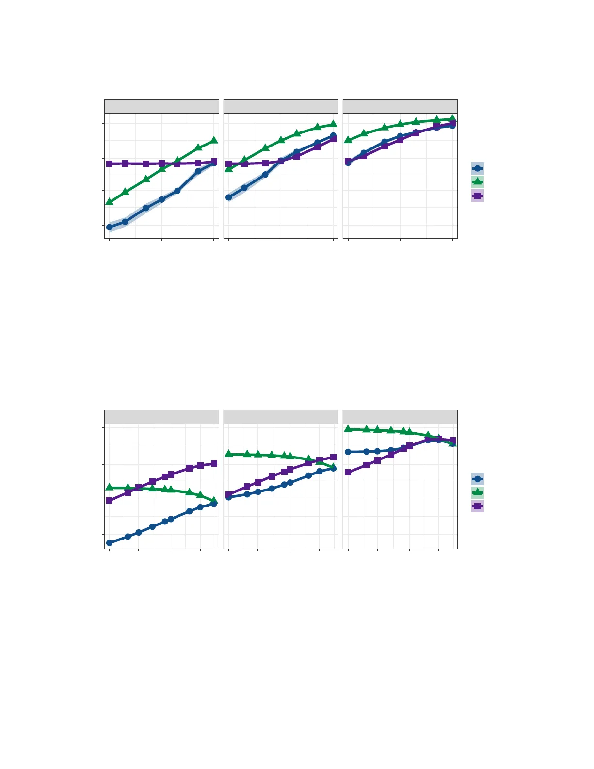
Adjacency Sp ectral Em b eddings of Correlation Net w orks Keith Levin Univ ersity of Wisconsin–Madison Abstract In man y applications, weigh ted netw orks are constructed based on time series data: eac h time series is associated to a vertex and edge w eigh ts are giv en b y pairwise cor- relations. The result is a net w ork whose edge dep endency structure violates the as- sumptions of most common net work mo dels. Nonetheless, it is common to analyze these “correlation netw orks” using embedding metho ds deriv ed from edge-indep enden t net work models, based on a belief that the edges are appro ximately indep enden t. In this work, we put this mo deling choice on ﬁrm theoretical ground. W e sho w that when the time series are expressible in terms of a small num b er of F ourier basis elemen ts (or in some other suitably-c hosen basis), correlation netw orks corresp ond to latent space net works with dep enden t edge noise in which the v ertex-lev el latent v ariables enco de the basis co eﬃcien ts. F urther, we show that when time series are observ ed sub ject to noise, sp ectral embedding of the resulting noisy correlation netw ork still recov ers these true vertex-lev el latent representations under suitable assumptions. This characteriza- tion of embeddings as learning F ourier co eﬃcients app ears to be folklore in the signal pro cessing communit y in the con text of principal comp onen t analysis, but is, to the b est of our knowledge, new to the statistical net work analysis literature. 1 In tro duction Net works ha v e emerged as crucial data sources in scien tiﬁc disciplines including neuroscience ( Sp orns 2012 ; V ogelstein et al. 2019 ), economics ( Elliot et al. 2014 ; T umminello et al. 2010 ), microbiomics ( Fierer 2017 ; Jiang et al. 2019 ) and so ciology ( Lazega 2001 ; Zh u et al. 2020 ) to name but a few. As a result, a handful of w orkhorse statistical net work mo dels hav e emerged. F or example, the sto c hastic blo ckmodel (SBM; Holland et al. 1983 ; Abb e 2018 ) p osits that eac h v ertex belongs to one of d comm unities, and the probabilit y that t wo vertices form an edge is fully determined b y their comm unity mem b erships, with edges generated indep enden tly conditional on comm unity mem b erships. In recent y ears, the SBM has b een extended in a v ariet y of w a ys (see, e.g., Karrer and Newman 2011 ; Airoldi et al. 2008 ; Sengupta and Chen 2018 ; Golden b erg et al. 2010 ; Gao et al. 2018 ; Zhang et al. 2020 ; Abb e 1 2018 ; Jin et al. 2024 ). F or example, the degree-corrected SBM ( Karrer and Newman 2011 ) mo diﬁes the SBM to giv e eac h v ertex a “popularity” parameter, so that v ertices from the same comm unit y ma y exhibit distinct b ehaviors in their propensity to form edges. Mo dels suc h as the random dot pro duct graph (RDPG; Y oung and Sc heinerman 2007 ; A threya et al. 2018 ; Rubin-Delanc hy et al. 2022 ), graph ro ot distribution ( Lei 2021 ), Hoﬀ-st yle mo dels ( Hoﬀ et al. 2002 ), and the graphon ( Lo v´ asz 2012 ; T ang and Cap e 2025 ) further extend this idea, mo deling net w ork structure as driv en b y laten t v ertex-level vectors. All of these mo dels and their attendan t estimation pro cedures rely on the assumption that edges are generated indep enden tly conditional on latent vertex-lev el structure. In many applications, these edge indep endence assumptions are grossly violated. Most notably , weigh ted net w orks are often derived from correlations b etw een time series: a time series or other sequence is associated to each vertex, and edge weigh ts are giv en by the correlations b et ween these sequences. I n these c orr elation networks , edge indep endence as- sumptions clearly fail to hold: the same time series app ears in all edge weigh ts incident up on a given v ertex. As an example, consider connectomic netw orks ( Sp orns 2012 ), in which v er- tices corresp ond to brain regions, and edge w eigh ts enco de the strength of in teraction b etw een brain regions. These in teraction strengths are t ypically measured by correlations betw een blo o d o xygen levels in these brain regions ( Mahadev an et al. 2021 ; Jin et al. 2025 ). Thus, man y connectomic net w orks are w eighted (or are binarized v ersions of w eigh ted net works; see Le et al. 2018 ; Masuda et al. 2025 , and citations therein), with edges given by correla- tions b etw een noisily-measured underlying signals from diﬀerent brain regions. As another example, consider aﬃnity matrices, which enco de net works whose v ertices are sto cks or other assets, and edges describe similarities of those assets ( F an et al. 2014 ; Hong and Xu 2019 ; F an et al. 2021 ), usually measured b y correlation across some set (e.g., correlation of prices or similarit y of in ternet searc h activit y). As y et another example, in microbiome studies, it is common to construct net works whose v ertices corresp ond to sp ecies of micro organisms, and edges capture the correlation of abundance coun ts across a collection of patien ts or en vironments ( Lee et al. 2020 ; Bec ker et al. 2023 ; Zitnik et al. 2024 ; Barylli et al. 2025 ). In all of these example settings, the net works under study ha ve w eighted edges, with w eights given by correlations b et ween sequences. F or a given v ertex, all edges inciden t on that v ertex are based on the same sequence’s correlations with all other observed sequences. F or ex ample, in connectomic netw orks, the blo o d oxygen lev els measured at brain region i are used to compute the edge weigh ts b etw een region i and all other brain regions. The result is that edges in this netw ork are clearly not indep endent, even after conditioning on any ob vious c hoice of latent structure. Despite this gap b et ween mo del assumptions and reality , indep enden t-edge laten t v ariable mo dels hav e b een applied to these and related application domains with clear success. The apparent consensus in the netw ork analysis communit y is that this violation of independence assumptions is not a concern. The goal of the present w ork is to put this folklore on ﬁrm ground b y studying the prop erties of these correlation net works. In particular, we focus here on the behavior of emb e ddings of correlation netw orks. Em b eddings, whereby vertices of a net w ork are represented in a lo w-dimensional Eu- clidean space ( Sussman et al. 2012 , 2014 ; T ang and Prieb e 2018 ; Gro ver and Lesk ov ec 2016 ), 2 are widely deplo y ed for analysis and visualization of netw ork data. Em b edding metho ds, b y and large, bring with them implicit mo deling assumptions. F or example, the adjacency spec- tral embedding (ASE; Sussman et al. 2012 ) implicitly assumes that the observed symmetric adjacency matrix A ∈ R n × n can b e written as a low-rank matrix sub ject to noise, A = X ⋆ X ⋆ ⊤ + E , (1) where the ro ws of X ⋆ ∈ R n × d enco de “laten t p ositions” of the n vertices, and the matrix E ∈ R n × n has mean-zero entries indep endent (up to symmetry) given X ⋆ . Similar ideas app ear in, for example, Rubin-Delanch y et al. ( 2022 ); Levin et al. ( 2017 ); Lei ( 2021 ); Levin et al. ( 2022 ); Gallagher et al. ( 2024 ). See A threya et al. ( 2018 ) for discussion of the RDPG, the mo del that motiv ates the ASE and related sp ectral em b eddings. More generally , em b eddings arise naturally in communit y detection as an input to k -means or other clustering metho ds to recov er communit y mem b erships in the sto chastic blo c kmo del ( Luxburg 2007 ; Rohe et al. 2011 ; Lyzinski et al. 2014 ; Prieb e et al. 2019 ; Lyzinski et al. 2017 ). In ligh t of the conditional indep endence assumptions on E , applying sp ectral em b edding metho ds to correlation matrices violates what are otherwise standard, albeit unrealistic, net work mo deling assumptions. Nonetheless, embeddings are used to analyze correlation or co v ariance netw orks throughout the sciences. The “folklore” b elief is that edge dep endence can be safely ignored b ecause the correlations are approximately indep enden t. An additional concern relates to the fact that netw ork em b eddings in edge-indep enden t mo dels can typically estimate a sensibly-deﬁned laten t structure. F or example, under suitable assumptions on E in Equation ( 1 ), the ASE of A recov ers X ⋆ , up to orthogonal non-iden tiﬁability (see Section 2 for further discussion). When one applies the ASE or some other em b edding method to a correlation netw ork, there is no obvious analogue of the low-rank structure X ⋆ in Equation ( 1 ) for the em b edding to estimate, nor is there an obvious interpretation for such a structure. This w ork sets out to address these concerns and put the “folklore” on ﬁrm ground. First, w e sho w that correlation net w orks ha ve a natural analogue of the lo w-dimensional laten t structure X ⋆ in Equation ( 1 ), which enco de the F ourier co eﬃcients of the time series (or the co eﬃcien ts under an y other suitably-c hosen transform). This is made formal in Lemmas 1 and 2 b elo w. Second, we sho w in Theorem 1 that when a collection of time series is observ ed sub ject to noise, the ASE applied to the correlation matrix reco v ers this lo w-dimensional encoding of the F ourier co eﬃcients, up to non-iden tiﬁabilit y constrain ts, at a rate that is qualitatively similar to those established for other related estimation problems. Notation. F or a p ositiv e integer n , w e write [ n ] = { 1 , 2 , . . . , n } . Throughout, matrices and v ectors are b olded, while scalars are in normal t yp eface. F or a matrix B , w e use B ⊤ to denote its transp ose and B H to denote its conjugate transp ose. W e write ∥ B ∥ for the sp ectral norm of B , ∥ B ∥ F for its F rob enius norm, and ∥ B ∥ 2 , ∞ for its (2 , ∞ )-norm, i.e., the maxim um Euclidean norm of the rows of B . W e denote the identit y matrix by I , the matrix of all ones by J and the matrix of all zeros b y 0 , with dimensions made clear by context. W e use i to denote the imaginary unit. Note that w e use the similar lo oking i in places, but only ev er as a summation index or subscript, so there is no risk of confusion. F or a complex n umber z ∈ C , we use ℜ ( z ) and ℑ ( z ) to denote its real and imaginary comp onents, resp ectiv ely , so that z = ℜ ( z ) + i ℑ ( z ). W e write ¯ z for the complex conjugate of z . 3 2 Mo del Setup and Main Results Consider a collection of n length- T discrete-time time series, so that for each i ∈ [ n ] and t ∈ [ T ], Z ⋆ i,t ∈ R is the v alue of the i -th time series at time t ∈ [ T ]. W e write Z ⋆ i ∈ R T to denote the i -th time series, written as a T -dimensional v ector. W e mo del these time series as sub ject to noise, so that our observ ed data takes the form Z i = Z ⋆ i + N i for eac h i ∈ [ n ], where N i ∈ R T is a v ector of measurement noise (precise noise assumptions are giv en in Section 2.2 ). F or example, in our neuroimaging example discussed in Section 1 , the true signal Z ⋆ i corresp onds to underlying brain activit y in the brain region indexed b y i ∈ [ n ], while the noisy signal Z i corresp onds to the measured blo o d oxygen lev el in brain region i . Collecting the true signals Z ⋆ i in to the rows of Z ⋆ ∈ R n × T and forming matrices Z ∈ R n × T and N ∈ R n × T analogously , we may write Z = Z ⋆ + N ∈ R n × T . (2) In the applications discussed in Section 1 , it is common to form a w eighted netw ork with v ertices i ∈ [ n ] by assigning edge weigh ts via correlation among these time series. That is, ignoring measuremen t noise for no w, we form a weigh ted netw ork with adjacency matrix R ⋆ =  R ⋆ i,j  =  Corr( Z ⋆ i , Z ⋆ j )  =  Co v ( Z ⋆ i , Z ⋆ j ) σ ⋆ i σ ⋆ j  ∈ R n × n , (3) where σ ⋆ i 2 = 1 T T X t =1 Z ⋆ i,t − 1 T T X s =1 Z ⋆ i,s ! 2 . (4) W e refer to a netw ork with adjacency matrix as in Equation ( 3 ) as a c orr elation network , in ligh t of the fact that its edge w eights enco de correlations b etw een time series. Remark 1. On ﬁrst glanc e, it is tempting to interpr et σ ⋆ i 2 as simply a varianc e. However, sinc e we interpr et Z ⋆ i ∈ R T as enc o ding network structur e, r ather than r andom noise, σ ⋆ i 2 is b etter viewe d as a me asur e of signal str ength. Inde e d, σ ⋆ i 2 c orr esp onds pr e cisely to the p ower in the signal Z ⋆ i after c entering ab out its time-aver age ( Opp enheim and Schafer 2009 ). Deﬁning the “cen tering” matrix M = 1 T ( I − J ) ∈ R T × T , (5) w e may write R ⋆ as a matrix pro duct, R ⋆ = 1 T Σ ⋆ − 1 / 2 Z ⋆ MZ ⋆ ⊤ Σ ⋆ − 1 / 2 , (6) where Σ ⋆ = diag  σ ⋆ 1 2 , σ ⋆ 2 2 , . . . , σ ⋆ n 2  ∈ R n × n . (7) 4 Of course, in practice, we do not observe the true signals in Z ⋆ , but instead observe Z as in Equation ( 2 ), and our resulting correlation net w ork has an adjacency matrix giv en by R = 1 T Σ − 1 / 2 ZMZ ⊤ Σ − 1 / 2 , (8) where Σ = diag  σ 2 1 , σ 2 2 , . . . , σ 2 n  ∈ R n × n (9) is the diagonal matrix of (noisy) v ariances, σ 2 i = 1 T T X t =1 Z i,t − 1 T T X s =1 Z i,s ! 2 . (10) In the applications in Section 1 , one observ es a collection of time series and forms a correlation netw ork with adjacency matrix as in Equation ( 3 ) or ( 8 ). W e then apply an em b edding method to this net work. Our goal in the presen t w ork is to address t wo questions: 1. Is there a sense in which R ⋆ is driven by a lo w-dimensional latent structure, analogous to the role play ed by X ⋆ in Equation ( 1 )? 2. Under what conditions does an embedding of the noisy correlation netw ork R in Equa- tion ( 8 ) reco ver this latent structure, and at what rate? Belo w, we address b oth of these questions as they pertain to the adjacency sp ectral em b edding. Giv en a net w ork with adjacency matrix A ∈ R n × n , the d -dimensional ASE pro duces an n -b y- d matrix whose ro ws enco de d -dimensional embeddings of the v ertices: ASE( A , d ) = V | D | 1 / 2 ∈ R n × d (11) where D ∈ R d × d is the diagonal matrix of the d largest-magnitude eigenv alues of A and V ∈ R n × d con tains as its columns the corresp onding eigenv ectors. Under a v ariety of netw ork mo dels, A can b e expressed as in Equation ( 1 ), and X ⋆ is naturally viewed as a lo w-rank structure underlying the observed netw ork. As suc h, X ⋆ is a natural target for estimation and inference. Of course, estimation of X ⋆ is p ossible only up to right-m ultiplication b y an orthogonal matrix, since for any Q ∈ O d , X ⋆ X ⋆ ⊤ = X ⋆ Q ( X ⋆ Q ) ⊤ . Under suitable assumptions on X ⋆ and E in Equation ( 1 ) (see, e.g., Lyzinski et al. 2014 ; A threya et al. 2018 ; Rubin-Delanc h y et al. 2022 ; Rohe et al. 2011 ; Levin et al. 2022 ; Gallagher et al. 2024 ), min Q ∈ O d ∥ ASE( A , d ) Q − X ⋆ ∥ 2 , ∞ = o P (1) . That is, the ASE reco v ers the latent structure X ⋆ , up to orthogonal non-iden tiﬁability , uniformly o v er the v ertices i ∈ [ n ]. Our goal is to identify a lo w-dimensional structure 5 analogous to X ⋆ that giv es rise to R ⋆ , and to sho w that the ASE of R ⋆ reco vers this structure (up to non-identiﬁabilit y constrain ts) under suitable assumptions. W e fo cus here on the ASE o wing to its comparative simplicit y , but w e anticipate that m uch of our analysis can b e extended to other sp ectral em b eddings and related metho ds (e.g., T ang and Prieb e 2018 ; Mo dell and Rubin-Delanc h y 2021 ; Rubin-Delanch y et al. 2022 ; Grov er and Lesk ov ec 2016 ; Lin et al. 2023 ; Shen et al. 2023 ; Zhang and T ang 2024 ). 2.1 Laten t structure in correlation net works T o understand the lo w-dimensional structure enco ded in R ⋆ , w e will aim to mimic the construction in Equation ( 1 ) and write R ⋆ = X ⋆ X ⋆ ⊤ for some choice of X ⋆ ∈ R n × d , where d ≪ n . T o ward this end, deﬁne e Z ⋆ = 1 √ T Σ ⋆ − 1 / 2 Z ⋆ M ∈ R n × T , (12) noting that the i -th row of this matrix, e Z ⋆ i ∈ R T , corresponds to a centered, normalized v ersion of the i -th observ ed time series Z ⋆ i ∈ R T . Since M is idemp otent, w e ma y rewrite Equation ( 3 ) as R ⋆ =  1 √ T Σ ⋆ − 1 / 2 Z ⋆ M   1 √ T Σ ⋆ − 1 / 2 Z ⋆ M  ⊤ = e Z ⋆ e Z ⋆ ⊤ . (13) Applying the discrete F ourier transform, w e can express, for an y i ∈ [ n ] and t ∈ [ T ], e Z ⋆ i,t = 1 T T X k =1 F ⋆ i,k exp  2 π i T ( k − 1)( t − 1)  , (14) where F ⋆ i,k denotes the ( k − 1)-th F ourier co eﬃcient of the i -th standardized time series e Z ⋆ i for eac h k ∈ [ T ]. That is, F ⋆ i,k = T X t =1 e Z ⋆ i,t exp  − 2 π i T ( k − 1)( t − 1)  . (15) W e note that under this conv ention, F ⋆ i, 1 is the F ourier co eﬃcient of e Z ⋆ i asso ciated to frequency zero, whic h is T times its mean. Since e Z ⋆ i is standardized, w e ha v e F ⋆ i, 1 = 0. Denote by Ω ∈ C T × T the (unitary) in verse discrete F ourier transform matrix, with en tries Ω k,t = 1 √ T exp  2 π i T ( k − 1)( t − 1)  , k , t ∈ [ T ] . Examining Equation ( 14 ), we see that we can express e Z ⋆ as e Z ⋆ = 1 √ T F ⋆ Ω . 6 Substituting this in to Equation ( 6 ), R ⋆ = 1 √ T F ⋆ Ω  1 √ T F ⋆ Ω  ⊤ = 1 √ T F ⋆ Ω  1 √ T F ⋆ Ω  H = 1 T F ⋆ F ⋆ H , (16) where the second equality follows from the fact that Z ⋆ is real and the last equality follo ws from the fact that Ω is unitary . Since F ⋆ enco des the F ourier transforms of real sequences, basic symmetry prop erties of the discrete F ourier transform ( Opp enheim and Sc hafer 2009 , Chapter 8), along with the fact that the rows of e Z ⋆ are cen tered, imply F ⋆ i,k = ( F ⋆ i,k = 0 if k = 1 F ⋆ i,T − k +2 if k ∈ { 2 , 3 , . . . , T } . (17) Deﬁne a matrix K ∈ R T × T according to K s,t =      1 if s = t = 1 1 if s + t = T + 2 0 otherwise, (18) and observe that b y Equation ( 17 ), F ⋆ H = ( F ⋆ K ) ⊤ . Substituting this in to Equation ( 16 ) and observing that K is a p ermutation matrix and th us has a square ro ot K 1 / 2 ∈ C T × T , R ⋆ = 1 T F ⋆ K 1 / 2  F ⋆ K 1 / 2  ⊤ , (19) Basic prop erties of the F ourier transform yield the follo wing result. A detailed pro of is given in App endix A . Lemma 1. If the matrix Z ⋆ has al l r e al entries, then so do es the matrix F ⋆ K 1 / 2 , and these entries ar e given by  F ⋆ K 1 / 2  i,k = ℜ  F ⋆ i,k  − ℑ  F ⋆ i,k  i ∈ [ n ] , k ∈ [ T ] . (20) In light of Lemma 1 and Equation ( 19 ), w e see that R ⋆ is indeed enco ded b y a low-rank structure if F ⋆ K 1 / 2 is lo w rank. Supp ose that there exist at most d 0 non-zero columns of F ⋆ . That is, supp ose that there exists a collection of d 0 F ourier basis elements whose span con tains all of the rows in e Z ⋆ . Equations ( 17 ) and ( 20 ) imply the existence of W ∈ O T suc h that the i -th ro w of F ⋆ K 1 / 2 W enco des, up to scaling, the real and imaginary parts of the F ourier co eﬃcien ts of e Z ⋆ i , and F ⋆ K 1 / 2 W has at most 2 d 0 non-zero columns. It follo ws that R ⋆ has rank d ≤ 2 d 0 , since from Equation ( 19 ), we hav e R ⋆ = 1 T F ⋆ K 1 / 2  F ⋆ K 1 / 2 W  ⊤ = 1 T F ⋆ K 1 / 2 W  F ⋆ K 1 / 2 W  ⊤ . 7 Th us, we may further write R ⋆ = U ⋆ Λ ⋆ U ⋆ ⊤ , (21) where Λ ⋆ = diag( λ ⋆ 1 , λ ⋆ 2 , . . . , λ ⋆ d ) con tains the d ≤ 2 d 0 non-zero eigen v alues of R ⋆ on its diagonal and U ⋆ ∈ R n × d has the d corresp onding orthonormal eigenv ectors as its columns. It follo ws that w e ma y deﬁne X ⋆ = U ⋆ Λ ⋆ 1 / 2 ∈ R n × d (22) to b e the “p opulation em b edding” of our (cen tered, scaled) time series data e Z ⋆ ∈ R n × T based on the correlation matrix R ⋆ , analogous to the low-rank matrix in Equation ( 1 ). Since X ⋆ X ⋆ ⊤ = U ⋆ Λ ⋆ U ⋆ ⊤ = R ⋆ = e Z ⋆ e Z ⋆ ⊤ =  1 √ T F ⋆ K 1 / 2   1 √ T F ⋆ K 1 / 2  ⊤ and all en tries of F ⋆ K 1 / 2 are real, there must exist f W ∈ O T suc h that  X ⋆ 0  = 1 √ T F ⋆ K 1 / 2 f W . W e hav e shown the following. Lemma 2. If the standar dize d time series in the r ows of e Z ⋆ ∈ R n × T c an b e r epr esente d in a d 0 -dimensional F ourier b asis, then ther e exists a d ≤ 2 d 0 and f W ∈ O T such that  ASE( R ⋆ , d ) 0  = 1 √ T F ⋆ K 1 / 2 f W . That is, the d -dimensional ASE of R ⋆ c orr esp onds pr e cisely to the F ourier r epr esentation of the signals in e Z ⋆ , up to ortho gonal non-identiﬁability. Said another w a y , Lemma 2 states that the F ourier coeﬃcients of the signals in e Z ⋆ corresp ond to a lo w-rank latent representation of the vertices in the correlation net w ork R ⋆ . Remark 2. While our discussion ab ove fo cuse d on r epr esenting the standar dize d time series e Z ⋆ in the F ourier b asis, the same b asic ar gument applies to any b asis that we might c onsider (e.g., wavelets or the discr ete c osine tr ansform). While we r estrict our attention to the F ourier b asis for the sake of c oncr eteness, our r esults and analysis ar e lar gely agnostic to this choic e of b asis. Key to our r esults is that ther e exist some unitary matrix Ω such that the r ows of e Z ⋆ Ω H enc o de the observe d time series in the chosen b asis. 2.2 Reco v ering lo w-dimensional laten t structure Lemmas 1 and 2 indicate that the noiseless correlation netw ork R ⋆ has a low-rank laten t structure given b y F ourier transforms of the time series in the ro ws of Z ⋆ . W e turn our atten tion now to the matter of recov ering this latent structure from R , the noisy version of R ⋆ , as given in Equation ( 8 ). F ollo wing previous w ork on netw ork embeddings ( Suss- man et al. 2012 ; Levin et al. 2017 ; T ang and Prieb e 2018 ; Levin et al. 2021 ), w e wish to 8 study the adjacency sp ectral embedding of the observed correlation matrix R as deﬁned in Equation ( 8 ). In particular, write R = UΛU ⊤ + U ⊥ Λ ⊥ U ⊤ ⊥ , (23) where Λ = diag( λ 1 , λ 2 , . . . , λ d ) con tains the d largest eigen v alues of R , U ∈ R n × d con tains the corresp onding orthonormal eigenv ectors as its columns, and Λ ⊥ = diag ( λ d +1 , λ d +2 , . . . , λ n ) and U ⊥ ∈ R n × ( n − d ) are deﬁned analogously for the trailing n − d eigenv alues. The d - dimensional ASE of the noisy correlation netw ork is then given by ˆ X = ASE( R , d ) = UΛ 1 / 2 ∈ R n × d , (24) and we ma y hop e that if the noise is not to o severe, ˆ X recov ers X ⋆ in Equation ( 22 ) up to non-iden tiﬁability . Of course, in practice, the dimension d is unknown and must b e selected from data. This mo del selection task is w ell-studied in the net works literature under latent space mo dels with conditionally indep endent edges (see, e.g., Chen and Lei 2018 ; Li et al. 2020 ; Han et al. 2023 ; Chakrabarty et al. 2025 ; T aing and Levin 2026 ). Myriad selection tec hniques for PCA and related dimensionality reduction metho ds ha v e also b een dev elop ed ( Joliﬀe 2002 ; Zh u and Gho dsi 2006 ), whic h may b e applicable as w ell. W e leav e a thorough exploration of this matter for future w ork, but App endix B includes an exp erimen tal in vestigation of the eﬀects of mo del missp eciﬁcation under the setting of Equation ( 2 ). Whether the ASE of R recov ers the latent structure X ⋆ dep end, of course, on the beha vior of the noise N = Z − Z ⋆ . W e assume comparativ ely little ab out the sp eciﬁc structure of N b ey ond ro w-wise indep endence. In particular, w e allo w for dependence within the ro ws of N , sub ject to tail deca y conditions. Assumption 1. The r ows N 1 , N 2 , . . . , N n ∈ R T of N ar e me an-zer o and indep endent, with n = O ( T ) . (25) F or e ach i ∈ [ n ] , N i is a ν i -sub gaussian r andom ve ctor ( V ershynin 2020 , Chapter 3). That is, for any ﬁxe d unit ve ctor u ∈ R T , the r andom variable u ⊤ N i is a ν i -sub gaussian r andom variable ( Boucher on et al. 2013 ; V ershynin 2020 ). Viewing the subgaussian parameter ν i as a proxy for the v ariance in the i -th row of N , our results require that the noise not ov erwhelm the signal carried in Z ⋆ . In particular, the threshold for this rate of growth is set b y the spectrum of the signal matrix R ⋆ . Deﬁning γ = min i ∈ [ n ] σ ⋆ i 2 ν i , (26) our results require that the condition num b er κ = λ ⋆ 1 /λ ⋆ d of R ⋆ not gro w too quickly with resp ect to γ and that the smallest signal eigen v alue λ ⋆ d is b ounded a wa y from zero. 9 Assumption 2. The signal eigenvalues λ ⋆ 1 ≥ λ ⋆ 2 ≥ · · · ≥ λ ⋆ d > 0 of the true c orr elation matrix R ⋆ ar e such that λ ⋆ d = Ω P (1) (27) and the c ondition numb er κ = λ ⋆ 1 /λ ⋆ d is such that κ = o ( T ) and κ log T γ = o (1) . (28) The following theorem c haracterizes how w ell the em b eddings of R recov er their p op- ulation counterparts. The result serv es as a correlation net work analogue of (2 , ∞ )-norm estimation error b ounds found in, for example, Sussman et al. ( 2012 ); Lyzinski et al. ( 2014 ); Rubin-Delanc hy et al. ( 2022 ); T ang and Prieb e ( 2018 ); Levin et al. ( 2022 ), whic h rely on edge indep endence assumptions. A pro of of this theorem can b e found in App endix F . Theorem 1. Under Assumptions 1 and 2 , let X ⋆ ∈ R n × d b e as in Equation ( 22 ) , and let ˆ X = ASE( R , d ) . Ther e exists Q ∈ O d such that min Q ∈ O d    ˆ X − X ⋆ Q    2 , ∞ ≤ C s d log T γ λ ⋆ d " 1 + κ κ s log n γ + r 1 T ! ∥ R ⋆ ∥ 2 , ∞ # It is instructiv e to consider the upp er b ound in Theor em 1 when κ and d are b oth b ounded ab o v e by constan ts. Using basic prop erties of the (2 , ∞ )-norm ( Cai and Zhang 2018 ; Cap e et al. 2019 ) and the fact that e Z ⋆ has standardized ro ws, w e ha ve ∥ R ⋆ ∥ 2 , ∞ = ∥ e Z ⋆ e Z ⋆ ⊤ ∥ 2 , ∞ ≤ ∥ e Z ⋆ ∥ 2 , ∞ ∥ Λ ⋆ 1 / 2 ∥ = p λ ⋆ 1 . It follo ws that when max { κ, d } = O (1), we can rewrite the b ound in Theorem 1 as min Q ∈ O d    ˆ X − X ⋆ Q    2 , ∞ ≤ C s log T γ s 1 λ ⋆ d + s log n γ + r 1 T ! , (29) and w e see that consisten t estimation o ccurs under Assumption 2 . Among previous work, most similar to the setting of Theorem 1 is the literature on heteroscedastic PCA, whic h considers a setting similar to Equation ( 2 ), where one observ es Z = Z ⋆ + N , and aims to recov er the left singular vectors of Z ⋆ . When the en tries within a row of N diﬀer in their v ariances, as w e allow in the presen t w ork, “v anilla” PCA fails due to bias in the diagonal entries of the empirical cov ariance matrix. Metho ds for correcting this bias include zeroing out the diagonal of the empirical co v ariance before computing its eigen vectors ( Abb e et al. 2022 ; Cai et al. 2021 ) and iterative approac hes that seek to impute or otherwise debias these diagonal en tries ( Zhang et al. 2022 ; Zhou and Chen 2025 ). Importantly , the estimation problem considered in Theorem 1 diﬀers from heteroscedastic PCA (and man y other related subspace estimation tasks) in its target of inference: w e aim to estimate the scaled leading eigenv ectors of R ⋆ (i.e., X ⋆ in Theorem 1 ; see also Lemma 2 ), while PCA 10 aims to estimate the left singular vectors of Z ⋆ . Given this diﬀerence, Theorem 1 cannot b e directly compared to results for heteroscedastic PCA. Nonetheless, it is informativ e to compare our assumptions with those used in this related literature. Zhang et al. ( 2022 ) consider the setting where the rows of Z ⋆ are dra wn i.i.d. from a distribution with rank- d co v ariance matrix ∆ 0 ∈ R T × T , and one observes Z = Z ⋆ + N where the ro ws of N are i.i.d. mean zero with indep enden t entries, but these en tries are allo wed to diﬀer in their v ariances. The goal is to estimate the signal eigenv ectors of ∆ 0 . Cai et al. ( 2021 ); Y an et al. ( 2024 ); Zhou and Chen ( 2025 ) consider a similar setting, with relaxed assumptions on the noise N more in line with the tail b ounds of our Assumption 1 , but still requiring en trywise indep endence in N . W e note that Cai et al. ( 2021 ); Y an et al. ( 2024 ) allo w for missing en tries in Z , which we do not consider here, though we exp ect that low-rank imputation metho ds as used in Li et al. ( 2020 ) can b e applied in the setting of Theorem 1 . Most similar in spirit to our assumptions are Abb e et al. ( 2022 ); Agterb erg et al. ( 2022 ), b oth of which allo w for dep endence within ro ws of N and impose tail bounds similar to our Assumption 1 . Both also require SNR-related assumptions that are sup erﬁcially similar to our Assumption 2 , but are in fact largely incomparable. Assumption 2 concerns γ , which measures ho w the signal present in individual rows of Z ⋆ , as measured b y σ ⋆ i 2 , compare to the v ariance-like quan tity ν i , which describ es the tail behavior of the i -th ro w of the noise matrix N . In contrast, Abb e et al. ( 2022 ); Agterb erg et al. ( 2022 ) measure SNR b y comparing λ ⋆ d to the v ariance of the noise (i.e., ν 1 , ν 2 , . . . , ν n in our notation). Abb e et al. ( 2022 ) and Agterb erg et al. ( 2022 ) also require assumptions on the coherence of the left singular v ectors of Z ⋆ . It is interesting to note that Theorem 1 requires no analogous assumptions on the eigenstructure of R ⋆ . Nor do es it require assumptions on how the cov ariances within the ro ws of N in teract with the signal eigenstructure, as required in Agterb erg et al. ( 2022 ). 3 Exp erimen ts W e turn no w to a brief exploration of our theoretical results. In particular, we are interested in verifying the estimation b ound in Theorem 1 , whic h predicts the rate at which ASE( R , d ) should reco v er X ⋆ once w e accoun t for orthogonal non-iden tiﬁability . When ev aluating an estimate Y ∈ R n × d of X ⋆ , we will tak e adv antage of the fact that, p er Lemma 2 , X ⋆ and e Z ⋆ are equal up to orthogonal rotation, and assess estimation error b y min W ∈ O T     Y 0  W − e Z ⋆    2 , ∞ , (30) where w e hav e app ended T − d columns of zeros to Y so that it is conformal with e Z ⋆ . In what follows, w e compare the ASE against tw o baseline metho ds for estimating e Z ⋆ . The ﬁrst is based on applying d -dimensional PCA to the cen tered matrix of time series ZM ∈ R n × T follo wed b y standardizing the rows. Note that we p erform a scaled PCA, with the eigenv ectors scaled by the square ro ots of the eigenv alues. In essence, this PCA-based estimate rev erses the steps of the ASE b y applying eigen v alue truncation b efor e p erforming 11 ro w normalization. Our second comparison is with a na ¨ ıv e metho d, whereby we simply use e Z = 1 √ T Σ − 1 / 2 ZM ∈ R n × T , as our estimate of e Z ⋆ . While suc h an estimate fails to yield dimensionality reduction the w ay that the ASE or other PCA-based metho ds migh t, it serv es as a baseline comparison to indicate whether an estimator is successfully removing noise from the observ ed signals. 3.1 Eﬀect of v ariance on estimation W e b egin by examining how the b eha vior of the rows of N inﬂuence estimation accuracy . F or a given n umber of vertices n , n umber of time series T , and a n um b er of signal frequen- cies d 0 < T / 2, we generate Z ⋆ b y c ho osing d 0 F ourier basis element indices from the set { 2 , 3 , . . . , ⌊ T / 2 ⌋} uniformly at random without replacement. Letting K denote this index set, for eac h i ∈ [ n ], w e generate Z ⋆ i b y p opulating the real and imaginary comp onents of the F ourier co eﬃcien ts indexed by K with i.i.d. dra ws from a standard normal. T o ensure that Z ⋆ has all real elemen ts, for each k ∈ K , we tak e the basis elemen t with index T − k + 2 to ha ve F ourier co eﬃcient equal to the complex conjugate of the co eﬃcient for index k , p er Equation ( 17 ) The result is that the n rows of Z ⋆ ∈ R n × T lie in the span of a d 0 -dimensional F ourier basis, and Z ⋆ has rank either 2 d 0 or 2 d 0 − 1, dep ending on the parit y of T and, if T is ev en, whether or not we ha ve selected the basis elemen t that is its own complex conjugate. Finally , w e rescale Z ⋆ so that ∥ Z ⋆ ∥ F = √ n . That is, Z ⋆ has av erage ro w norm equal to one. Our upp er b ound in Theorem 1 dep ends on the v ariance of the rows of N via the param- eter γ deﬁned in Equation ( 26 ), whic h captures the minim um, ov er all i ∈ [ n ], of the ratio of p o w er in Z ⋆ i ∈ R T to the v ariance-like parameter ν i . T o explore the eﬀect of γ , w e generate eac h ro w N i of N i ∈ [ n ], b y drawing the en tries of N i i.i.d. according to a mean zero normal with v ariance ν ∥ Z ⋆ i ∥ 2 . Under this setup, the ratio ν i /σ ⋆ i 2 is constant ov er all i ∈ [ n ] and w e ha v e γ = ν . W e ev aluate the (2 , ∞ )-norm b etw een our estimates and e Z ⋆ after the b est Pro crustes alignment, as in Equation ( 30 ). W e rep eated this pro cedure 50 times for each com bination of conditions. The results of this exp eriment are display ed in Figure 1 , which sho ws (2 , ∞ )-norm error as a function of the v ariance parameter ν for sev eral c hoices of d 0 . Examining the ﬁgure, we observ e that the ASE out-p erforms b oth our “na ¨ ıv e” baseline and the row-normalized PCA estimate, with the largest gap holding at low er noise lev els (i.e., low er entrywise v ariance) and low er v alues of d 0 . Most imp ortantly , we note that the b eha vior of the (2 , ∞ )-norm error with respect to the en trywise v ariance matches the rate predicted by Theorem 1 . Noting that γ = 1 /ν in the presen t setting, w e see that estimation error deca ys approximately as the square ro ot of 1 /γ for all four c hoices of d 0 . The quan tity γ in Theorem 1 is deﬁned as a minim um ov er all i ∈ [ n ] of an SNR-lik e quan tity . This raises the question as to whether the minim um in fact driv es the conv ergence rate. T o assess this, we mo dify the exp eriment describ ed ab ov e so that one randomly-c hosen ro w i 0 ∈ [ n ] of N is generated with entries i.i.d. from a mean zero normal with v ariance αν ∥ Z ⋆ i 0 ∥ 2 . When α = 1, we recov er the exp eriment from Figure 1 . Increasing α the v ariance 12 10 20 30 50 1e−04 1e−02 1e+00 1e−04 1e−02 1e+00 1e−04 1e−02 1e+00 1e−04 1e−02 1e+00 0.03 0.10 0.30 1.00 Entr ywise variance (log scale) (2, ∞ )−norm error (log scale) Method ASE baseline PCA Figure 1: Estimation error in (2 , ∞ )-norm as a function of v ariance parameter ν b y the ASE (blue circles), PCA (purple squares) and the na ¨ ıv e baseline (green triangles), when applied to n = 200 time series of length T = 200 for four choices of F ourier basis size d 0 = 10 , 20 , 30 , 50. of the i 0 -th ro w of N compared to the rest, and decreases γ . With n = 200 , T = 500 and d 0 = 20, we p erformed this exp erimen t for ν = 10 − 6 , 10 − 5 and 10 − 4 and v arying choices of α , with 50 Monte Carlo trials for each com bination of conditions. Figure 2 summarizes the results, sho wing (2 , ∞ )-norm estimation error as a function of the inﬂation factor α . When ν is not to o big (i.e., the left and middle plots), ASE estimation error increases as approximately the square ro ot of α , in line with the predictions of Theorem 1 . Examining the righ t- most subplot, whic h corresp onds to higher entrywise v ariance ν , w e see that p erformance degrades nearly to the point of b eing indistinguishable from the na ¨ ıve baseline, with the ASE and PCA-based metho d p erforming similarly p o orly . Additional exp eriments exploring the eﬀect of Gaussian versus Laplacian noise are presented in App endix B . 3.2 Eﬀect of dimension The rate in Theorem 1 suggests that the ASE estimation error should also dep end on the mo del dimension (i.e., t wice the n um b er of signal frequencies d 0 ), with estimation error gro wing as √ d 0 . T o inv estigate this, w e con tinue with the same experimental setup as the experiment in Figure 1 , this time with ﬁxed net work size n = 1200 and time series length T = 1800, and v arying the num b er of signal frequencies d 0 . F or each combination of conditions, we p erformed 50 indep ednet Monte Carlo trials and recorded the mean (2 , ∞ )- estimation error. The results of this exp erimen t is summarized in Figure 3 for three diﬀeren t c hoices of noise v ariance ν . W e see that at higher v ariances (i.e., ν = 0 . 001 on the right), none of our three estimation metho ds p erform esp ecially w ell, but at lo wer v ariances, the ASE outp erforms b oth the PCA-based metho d and the na ¨ ıve baseline, with estimation error ob eying the √ d -rate predicted b y our theory . 13 1e−06 1e−05 1e−04 1 10 100 1 10 100 1 10 100 0.03 0.10 0.30 1.00 V ar iance factor α (log scale) (2, ∞ )−norm error (log scale) Method ASE baseline PCA Figure 2: Estimation error in (2 , ∞ )-norm as a function of v ariance factor α by the ASE (blue circles), PCA (purple squares) and the na ¨ ıve baseline (green triangles), as applied to n = 200 time series of length T = 500 with F ourier basis size d 0 = 20. Shad ed regions indicate t wo standard errors of the mean. 1e−05 1e−04 0.001 10 30 100 300 10 30 100 300 10 30 100 300 0.03 0.10 0.30 1.00 T rue number of frequency components d 0 (log scale) (2, ∞ )−norm error (log scale) Method ASE baseline PCA Figure 3: Estimation error in (2 , ∞ )-norm as a function of the n umber of frequencies d 0 for ASE (blue circles), PCA (purple squares) and na ¨ ıv e baseline (green triangles), when applied to n = 1200 time series of length T = 1800 under three diﬀeren t c hoices of noise v ariance ν . 14 3.3 Eﬀect of sp ectrum of R ⋆ Examining the b ound in Theorem 1 , the estimation rate is inﬂuenced b y λ ⋆ d , the smallest signal eigenv alue in R ⋆ . Th us, we wish to conduct a n umerical exp eriment similar to those ab o v e, this time v arying λ ⋆ d while k eeping other mo del parameters ﬁxed. Ideally , this w ould include the condition n umber κ of R ⋆ . Unfortunately , the fact that e Z ⋆ ha ve unit-norm rows complicates suc h an exp eriment. By construction, the rows of e Z ⋆ are all unit norm, and b y Lemma 2 , w e hav e ∥ e Z ⋆ ∥ 2 F = P d k =1 λ ⋆ k . Th us, with λ ⋆ 1 = λ ⋆ 2 = · · · = λ ⋆ d , so that κ = 1, the num b er of v ertices n and the n umber of signal eigenv alues d completely determines λ ⋆ d (and all other eigen v alues of R ⋆ ). A further c hallenge arises from the fact that suc h an exp erimen t requires that w e generate e Z ⋆ not only to ha v e all d singular v alues the same, but to ha ve row sums equal to 0 and all rows with the same norm. Rather than trying to satisfy all of these constrain ts exactly , we generate the rows of Z ⋆ as in the previous t w o exp erimen ts, but standardize them so that Z ⋆ = e Z ⋆ In practice, so long as the num b er of signal frequencies d 0 is not large, this rarely yields a condition n umber larger than 5, so that, at least for the purp oses of asymptotics, we ma y treat n/d as equal to λ ⋆ d . Note that under this setting, for a ﬁxed mo del rank d , increasing n is equiv alent to increasing λ ⋆ d . Once w e hav e generated Z ⋆ , w e dra w the en tries of the noise N i.i.d. from a mean zero normal with v ariance ν = 1 e − 4 and construct Z = Z ⋆ + N . Note that o wing to our normalization constraint on Z ⋆ in this exp eriment, this v ariance is not directly comparable to that used in our ﬁrst tw o exp erimen ts. The results of this experiment are displa yed in Figure 4 . Examining the ﬁgure, we see that the b ehavior of the ASE is consistent with the Theorem 1 . When κ is constant, Equation ( 29 ) shows that increasing λ ⋆ d is not suﬃcien t to ensure con vergence of the ASE without also allo wing γ and T to grow, both of which are held ﬁxed in this exp eriment. W e note that this problem setting is artiﬁcially easy for the PCA-based metho d. Since the ro ws of Z ⋆ are already normalized, the PCA-based metho d is, in essence, just a truncation of Z . As such, it is not surprising that the PCA-based method con verges at a 1 / p λ ⋆ d rate in this exp erimen t. 4 Discussion and Conclusion Net work embedding metho ds with implicit edge indep endence assumptions are frequently ap- plied to correlation netw orks that clearly violate edge indep endence. Practitioners nonethe- less frequen tly apply these metho ds to correlation netw orks, under the in tuition that the dep endence among the edges is ignorable. W e ha v e presen ted an analysis of the b ehav- ior of sp ectral em b eddings as applied to correlation net w orks that puts this intuition on ﬁrm ground. W e hav e sho wn that correlation netw orks built from collections of time series ha ve a clear interpretation as having laten t p ositions enco ding the F ourier co eﬃcients of the time series, and w e ha v e sho wn that when noisily-observ ed time series are used to build a correlation net work, the ASE pro v ably recov ers the true underlying low-rank structure. There are several interesting directions for future w ork. W e conjecture that the rate in Theorem 1 is minima optimal, up to logarithmic factors and dependence on the condition 15 5 10 20 100 300 1000 100 300 1000 100 300 1000 0.1 0.2 0.3 Number of time series (log scale) (2, ∞ )−norm error (log scale) Method ASE baseline PCA Figure 4: Estimation error in (2 , ∞ )-norm as a function of the num b er of time series n by the ASE (blue circles), PCA (purple squares) and the na ¨ ıv e baseline (green triangles), as applied to time series of length T = 1000 under three diﬀeren t choices of d 0 . n umber κ . Establishing a minimax low er b ound is the fo cus of ongoing follo w-up w ork, starting from the argumen ts dev elop ed in Y an and Levin ( 2023 , 2024 ). W e expect that the dep endence on κ can b e relaxed, and p erhaps remo v ed entirely , with suitably careful b o okkeeping (see, e.g., P ensky 2024 ). If dep endence on κ cannot b e eliminated, future w ork should in vestigate whether approac hes similar to Zhou and Chen ( 2025 ) can b e used as a prepro cessing step to remo ve the eﬀect of condition num b er. As alluded to when comparing our results to the heteroscedastic PCA literature, it is in teresting to note that Theorem 1 do es not suggest a bias in tro duced b y heteroscedasticit y in the ro ws of N . F uture work should more carefully analyze how, if at all, heteroscedasticit y contributes to the estimation rate in Theorem 1 and whether, in the even t that there is structure present in the eigenv ec- tors of R ⋆ (i.e., the left singular v ectors of e Z ⋆ ), this structure can b e lev eraged to ac hieve impro ved estimation, analogously to recent results in low-rank matrix estimation under in- dep enden t noise ( Y an and Levin 2024 , 2025 ). Finally , as discussed in Section 2 , em b eddings of correlation net w orks and PCA applied directly to Z ⋆ b oth pro v ably learn low-rank rep- resen tations of the time series. F uture work should c haracterize when one or the other of these t w o metho ds is preferable, analogous to the study in ( Prieb e et al. 2019 ) comparing the ASE to the Laplacian sp ectral embedding ( T ang and Prieb e 2018 ). Ac knowledgemen ts. The author w ould like to thank Jes ´ us Arro y o, Av anti A threya, Nathan Aviles, Joshua Cap e, Alex Hay es, Elizav eta Levina, Zachary Lubb erts, Vince Lyzin- ski, Karl Rohe, Joseph Salzer, Ro ddy T aing, Hao Y an, W en Zhou, Ji Zhu and the attendees of the UW-Madison IFDS Seminar for helpful discussions and suggestions that ha ve greatly impro ved this pap er. The author was supp orted in part b y the Universit y of Wisconsin- Madison, Oﬃce of the Vice Chancellor for Research and Graduate Education with funding 16 from the Wisconsin Alumni Research F oundation. References E. Abb e. Comm unity detection and sto c hastic blo ck mo dels: Recent developmen ts. Journal of Machine L e arning R ese ar ch , 18(177):1–86, 2018. E. Abb e, J. F an, and K. W ang. An ℓ p theory of PCA and sp ectral clustering. The A nnals of Statistics , 50(4):2359–2385, 2022. J. Agterb erg, Z. Lubb erts, and C. E. Prieb e. En trywise estimation of singular v ectors of low- rank matrices with heterosk edasticity and dependence. IEEE T r ansactions on Information The ory , 68(7):4618–4650, 2022. E. M. Airoldi, D. M. Blei, S. E. Fienberg, and E. P . Xing. Mixed Mem b ership Sto chastic Blo c kmo dels. Journal of Machine L e arning R ese ar ch , 9:1981–2014, 2008. A. Athrey a, D. E. Fishkind, M. T ang, C. E. Prieb e, Y. P ark, J. T. V ogelstein, K. Levin, V. Lyzinski, Y. Qin, and D. L. Sussman. Statistical inference on random dot pro duct graphs: a survey . Journal of Machine L e arning R ese ar ch , 18:1–92, 2018. M. Barylli, J. Saha, T. E. Buﬀart, J. Koster, K. J. Lenos, L. V ermeulen, and V. M. Sher- aton. Biological m ulti-la yer and single cell netw ork-based multiomics mo dels – a review. arXiv:2503.09568 , 2025. M. Beck er, H. Nassar, C. Espinosa, I. A. Stelzer, D. F ey aerts, E. Berson, N. H. Bidoki, A. L. Chang, et al. Large-scale correlation netw ork construction for unrav eling the co ordination of complex biological systems. Natur e Computational Scienc e , 3:346–359, 2023. R. Bhatia. Matrix Analysis , v olume 169 of Gr aduate T exts in Mathematics . Springer Science & Business Media, 1997. S. Bouc heron, G. Lugosi, and P . Massart. Conc entr ation Ine qualities: A Nonasymptotic The ory of Indep endenc e . Oxford Universit y Press, 2013. C. Cai, G. Li, Y. Chi, H. V. P o or, and Y. Chen. Subspace estimation from unbalanced and incomplete data matrices: ℓ 2 , ∞ statistical guarantees. The A nnals of Statistics , 49(2): 944–967, 2021. T. T. Cai and A. Zhang. Rate-optimal p erturbation bounds for singular subspaces with applications to high-dimensional statistics. The Annals of Statistics , 46(1):60–89, 2018. J. Cap e, M. T ang, and C. E. Prieb e. The t w o-to-inﬁnity norm and singular subspace ge- ometry with applications to high-dimensional statistics. The A nnals of Statistics , 47(5): 2405–2439, 2019. 17 S. Chakrabart y , S. Sengupta, and Y. Chen. Netw ork cross-v alidation and mo del selection via subsampling. , 2025. K. Chen and J. Lei. Net w ork cross-v alidation for determining the num b er of communities in net work data. Journal of the Americ an Statistic al Asso ciation , 113(521):241–251, 2018. Y. Chen, Y. Chi, J. F an, and C. Ma. Sp e ctr al metho ds for data scienc e: A statistic al p ersp e ctive . F oundations and T rends in Mac hine Learning. No w Publishers, Inc., 2021. C. Davis and W. M. Kahan. The rotation of eigen vectors b y a p erturbation. SIAM Journal of Numeric al Analysis , 7(1), 1970. M. Elliot, B. Golub, and M. O. Jackson. Financial net w orks and con tagion. A meric an Ec onomic R eview , 104(10):3115–3153, 2014. J. F an, Y. Ke, and Y. Liao. Augmen ted factor mo dels with applications to v alidating mark et risk factors and forecasting b ond risk premia. Journal of Ec onometrics , 222(1):269–294, 2021. Y. F an, N. F outz, G. James, and W. Jank. F unctional resp onse additive mo del estimation with online virtual sto c k markets. The Annals of Applie d Statistics , 8:2435–2460, 2014. N. Fierer. Em bracing the unknown: disen tangling the complexities of the soil microbiome. Natur e R eviews Micr obiolo gy , 15(10):579–590, 2017. I. Gallagher, A. Jones, A. Bertiger, C. E. Prieb e, and P . Rubin-Delanc hy . Sp ectral embedding of weigh ted graphs. Journal of the Americ an Statistic al Asso ciation , 119(547):1923–1932, 2024. C. Gao, Z. Ma, A. Y. Zhang, and H. H. Zhou. Comm unity detection in degree-corrected blo c k mo dels. The Annals of Statistics , 46(5):2153–2185, 2018. A. Golden b erg, A. X. Zheng, S. E. Fien b erg, and E. M. Airoldi. A surv ey of statistical net work mo dels. F oundations and T r ends in Machine L e arning , 2:129–233, 2010. A. Grov er and J. Lesko vec. no de2vec: Scalable feature learning for netw orks. In Pr o c e e dings of the 22nd ACM SIGKDD International Confer enc e on Know le dge Disc overy and Data Mining , pages 855–864, 2016. X. Han, Q. Y ang, and Y. F an. Universal rank inference via residual subsampling with application to large netw orks. The Annals of Statistics , 51(3):1109–1133, 2023. P . D. Hoﬀ, A. E. Raftery , and M. S. Handco ck. Laten t space approaches to so cial netw ork analysis. Journal of the Americ an Statistic al Asso ciation , 97(460):1090–1098, 2002. P . W. Holland, K. B. Lask ey , and S. Leinhardt. Sto chastic blo c kmo dels: First steps. So cial Networks , 5(2):109–137, 1983. 18 H. Hong and J. Xu. Inferring laten t so cial net w orks from stock holdings. Journal of Financial Ec onomics , 131(2):323–344, 2019. D. Jiang, C. R. Armour, C. Hu, M. Mei, C. Tian, T. J. Sharpton, and Y. Jiang. Microbiome m ulti-omics netw ork analysis: Statistical considerations, limitations, and opp ortunities. F r ontiers in Genetics , 10, 2019. H. Jin, J. S. B. Ramirez, K. Byeon, B. E. Russ, A. F alc hier, G. Linn, G. Kiar, C. E. Sc hro eder, J. T. V ogelstein, M. P . Milham, and T. Xu. Is Pearson’s correlation co eﬃcien t enough for functional connectivit y in fMRI? Imaging Neur oscienc e , 2025. J. Jin, Z. T. Ke, and S. Luo. Mixed membership estimation for so cial netw orks. Journal of Ec onometrics , 239(2):105369, 2024. I. T. Joliﬀe. Princip al Comp onent Analysis . Springer Series in Statistics. Springer, 2nd edition, 2002. B. Karrer and M. E. J. Newman. Sto c hastic blockmodels and communit y structure in net works. Physic al R eview E , 83(1):016107, 2011. E. Lazega. The Col le gial Phenomenon: The So cial Me chanisms of Co op er ation Among Pe ers in a Corp or ate L aw Partnership . Oxford Universit y Press, 2001. C. M. Le, K. Levin, and E. Levina. Estimating a netw ork from m ultiple noisy realizations. Ele ctr onic Journal of Statistics , 12(2):4697–4740, 2018. B. Lee, S. Zhang, A. P oleksic, and L. Xie. Heterogeneous Multi-Lay ered Netw ork Mo del for Omics Data In tegration and Analysis. F r ontiers in Genetics , 10, 2020. J. Lei. Net work represen tation using graph ro ot distributions. The Annals of Statistics , 49 (2):745–768, 2021. K. Levin, A. A threya, M. T ang, V. Lyzinski, Y. P ark, and C. E. Prieb e. A cen tral limit theorem for an omnibus embedding of random dot pro duct graphs. , 2017. K. Levin, F. Ro osta, M. T ang, M. W. Mahoney , and C. E. Prieb e. Limit theorems for out-of-sample extensions of the adjacency and laplacian sp ectral em b eddings. Journal of Machine L e arning R ese ar ch , 22(194):1–59, 2021. K. Levin, A. Lo dhia, and E. Levina. Reco vering shared structure from m ultiple net w orks with unkno wn edge distributions. Journal of Machine L e arning R ese ar ch , 23:1–48, 2022. T. Li, E. Levina, and J. Zhu. Net w ork cross-v alidation by edge sampling. Biometrika , 107 (2):257–276, 2020. 19 C. Lin, D. L. Sussman, and P . Ishw ar. Ergo dic limits, relaxations, and geometric prop erties of random walk no de embeddings. IEEE T r ansactions on Network Scienc e and Engine ering , 10(1):346–359, 2023. L. Lo v´ asz. L ar ge Networks and Gr aph Limits . American Mathematical So ciet y , 2012. U. V on Luxburg. A tutorial on sp ectral clustering. Statistics and c omputing , 17(4):395–416, 2007. V. Lyzinski, D. L. Sussman, M. T ang, A. A threy a, and C. E. Prieb e. P erfect clustering for sto c hastic blo ckmodel graphs via adjacency sp ectral embedding. Ele ctr onic Journal of Statistics , 8(2):2905–2922, 2014. V. Lyzinski, M. T ang, A. A threya, Y. P ark, and C. E. Prieb e. Communit y detection and clas- siﬁcation in hierarchical sto chastic blo c kmo dels. IEEE T r ansactions on Network Scienc e and Engine ering , 2017. A. S. Mahadev an, U. A. T o oley , M. A. Bertolero, A. P . Mac key , and D. S. Bassett. Ev aluating the sensitivity of functional connectivity measures to motion artifact in resting-state fmri data. Neur oImage , 241:118408, 2021. ISSN 1053-8119. N. Masuda, Z. M. Bo yd, D. Garlaschelli, and P . J. Muc ha. Introduction to correlation net works: In terdisciplinary approac hes b eyond thresholding. Physics R ep orts , 1136:1–39, 2025. A. Mo dell and P . Rubin-Delanc hy . Sp ectral clustering under degree heterogeneit y: a case for the random walk Laplacian. , 2021. A. V. Oppenheim and R. W. Sc hafer. Discr ete Time Signal Pr o c essing . Pearson, 3rd edition, 2009. M. P ensky . Da vis-Kahan theorem in the tw o-to-inﬁnity norm and its application to p erfect clustering. , 2024. C. E. Prieb e, J. T. V ogelstein, J. M. Conro y , M. T ang, A. Athrey a, J. Cap e, and E. Bridge- ford. On a tw o-truths phenomenon in sp ectral graph clustering. Pr o c e e dings of the National A c ademy of Scienc es , 116(13):5995–6000, 2019. K. Rohe, S. Chatterjee, and B. Y u. Sp ectral clustering and the high-dimensional sto c hastic blo c kmo del. The Annals of Statistics , 39(4):1878–1915, 2011. P . Rubin-Delanc hy, J. Cap e, M. T ang, and C. E. Priebe. A statistical in terpretation of sp ectral em b edding: The generalised random dot pro duct graph. Journal of the R oyal Statistic al So ciety: Series B (Statistic al Metho dolo gy) , 84(4):1446–1473, 2022. S. Sengupta and Y. Chen. A blo ck mo del for no de p opularity in net works with comm unity structure. Journal of the R oyal Statistic al So ciety Series B , 80:365–386, 2018. 20 C. Shen, Q. W ang, and C. E. Prieb e. One-hot graph enco der em b edding. IEEE T r ansactions on Pattern Analysis and Machine Intel ligenc e , 45(6):7933–7938, 2023. O. Sp orns. Disc overing the Human Conne ctome . MIT Press, 2012. D. L. Sussman, M. T ang, D. E. Fishkind, and C. E. Priebe. A consisten t dot pro duct em b ed- ding for sto c hastic blo ckmodel graphs. Journal of the A meric an Statistic al Asso ciation , 107(499):1119–1128, 2012. D. L. Sussman, M. T ang, and C. E. Prieb e. Consistent laten t p osition estimation and vertex classiﬁcation for random dot pro duct graphs. IEEE T r ansactions on Pattern Analysis and Machine Intel ligenc e , 36(1):48–57, 2014. R. T aing and K. Levin. On the eﬀect of missp ecifying the em b edding dimension in lo w-rank net work mo dels. , 2026. M. T ang and J. R. Cap e. Eigenv ector ﬂuctuations and limit results for random graphs with inﬁnite rank k ernels. , 2025. M. T ang and C. E. Prieb e. Limit theorems for eigen v ectors of the normalized laplacian for random graphs. The Annals of Statistics , 46(5):2360–2415, 2018. M. T umminello, F. Lillo, and R. N. Man tegna. Correlation, hierarchies, and net w orks in ﬁnancial mark ets. Journal of Ec onomic Behavior & Or ganization , 75(1):40–58, 2010. Roman V ershynin. High-Dimensional Pr ob ability: A n Intr o duction with Applic ations in Data Scienc e . Cam bridge Universit y Press, 1st edition, 2020. J. T. V ogelstein, E. W. Bridgeford, B. D. P edigo, J. Ch ung, K. Levin, B. Mensh, and Carey E Prieb e. Connectal coding: disco vering the structures linking cognitiv e phenot yp es to individual histories. Curr ent Opinion in Neur obiolo gy , 55:199–212, 2019. H. Y an and K. Levin. Minimax rates for laten t position estimation in the generalized random dot pro duct graph. , 2023. H. Y an and K. Levin. Coherence-free en trywise estimation of eigenv ectors in low-rank signal- plus-noise matrix models. In A. Glob erson, L. Mack ey , D. Belgrav e, A. F an, U. Paquet, J. T omczak, and C. Zhang, editors, A dvanc es in Neur al Information Pr o c essing Systems , v olume 37, pages 126566–126619, 2024. H. Y an and K. Levin. Impro ved dep endence on coherence in eigenv ector and eigenv alue estimation error b ounds. In Twenty-Ninth Annual Confer enc e on Artiﬁcial Intel ligenc e and Statistics (AIST A TS) , 2025. Y. Y an, Y. Chen, and J. F an. Inference for heterosk edastic PCA with missing data. The A nnals of Statistics , 52(2):729–756, 2024. 21 S. Y oung and E. Sc heinerman. Random dot product graph mo dels for so cial netw orks. In Pr o c e e dings of the 5th International Confer enc e on A lgorithms and mo dels for the web- gr aph , pages 138–149, 2007. A. R. Zhang, T. T. Cai, and Y. W u. Heteroskedastic PCA: Algorithm, optimalit y , and applications. The Annals of Statistics , 50(1):53–80, 2022. Y. Zhang and M. T ang. A theoretical analysis of DeepW alk and no de2vec for exact recov ery of comm unity structures in sto chastic blo c kmo dels. IEEE T r ansactions on Pattern Analysis and Machine Intel ligenc e , 46(2):1065–1078, 2024. Y. Zhang, E. Levina, and J. Zhu. Detecting o v erlapping comm unities in netw orks using sp ectral metho ds. SIAM Journal on Mathematics of Data Scienc e , 2(2):265–283, 2020. Y. Zhou and Y. Chen. Deﬂated HeteroPCA: Ov ercoming the curse of ill-conditioning in heterosk edastic PCA. The Annals of Statistics , 53(1):91–116, 2025. M. Zhu and A. Gho dsi. Automatic dimensionalit y selection from the scree plot via the use of proﬁle lik eliho o d. Computational Statistics & Data Analysis , 51(2):918–930, 2006. X. Zh u, D. Huang, R. Pan, and H. W ang. Multiv ariate spatial autoregressive model for large scale so cial net works. Journal of Ec onometrics , 215(2):591–606, 2020. M. Zitnik, M. M. Li, A. W ells, K. Glass, D. M. Gysi, A. Krishnan, T. M. Murali, P . Radiv o jac, S. Ro y , A. Baudot, et al. Current and future directions in net work biology . Bioinformatics advanc es , 4(1):vbae099, 2024. 22 A F ourier Co eﬃcien ts and Lo w-Rank T runcation of R ⋆ Here we pro ve Lemma 1 , which implies that we ma y in terpret the low-rank truncation of a correlation matrix as capturing the F ourier co eﬃcien ts of the time series, up to orthogonal rotation. W e remind the reader that K ∈ R T × T denotes the matrix deﬁned in Equation ( 18 ). Pr o of of L emma 1 . W e begin b y noting that b y construction, Ke 1 = e 1 , and for all ℓ ∈ { 2 , 3 , . . . , T } , Ke ℓ = e T − ℓ +2 . It follows that K has eigendecomp osition K = e 1 e ⊤ 1 + ⌈ ( T − 1) / 2 ⌉ X ℓ =2 ( e ℓ + e T − ℓ +2 ) ( e ℓ + e T − ℓ +2 ) ⊤ ∥ e ℓ + e T − ℓ +2 − ⌊ ( T − 1) / 2 ⌋ X ℓ =2 ( e ℓ − e T − ℓ +2 ) ( e ℓ − e T − ℓ +2 ) ⊤ ∥ e ℓ − e T − ℓ +2 ∥ , and th us we can construct the square ro ot of K according to K 1 / 2 = e 1 e ⊤ 1 + ⌈ ( T − 1) / 2 ⌉ X ℓ =2 ( e ℓ + e T − ℓ +2 ) ( e ℓ + e T − ℓ +2 ) ⊤ ∥ e ℓ + e T − ℓ +2 ∥ + ⌊ ( T − 1) / 2 ⌋ X ℓ =2 i ( e ℓ − e T − ℓ +2 ) ( e ℓ − e T − ℓ +2 ) ⊤ ∥ e ℓ − e T − ℓ +2 ∥ . (31) Recall from Equation ( 15 ) that the ro ws of F ⋆ enco de the F ourier co eﬃcients of the corresp onding ro ws of Z ⋆ , whic h is assumed to hav e all real en tries. Since the rows of e Z ⋆ are cen tered by construction, we hav e F ⋆ i, 1 = T X t =1 e Z ⋆ i,t = 0 (32) for all i ∈ [ n ], so that F ⋆ e 1 e ⊤ 1 = 0 . (33) On the other hand, recalling Equation ( 17 ), for all i ∈ [ n ] and ℓ ∈ { 2 , 3 , . . . , T } , F ⋆ i,ℓ = F ⋆ i,T − ℓ +2 . (34) It follo ws that for an y i ∈ [ n ] and an y ℓ ∈ { 2 , 3 , . . . , ⌊ ( T − 1) / 2 ⌋} ,  F ⋆ + F ⋆  ( e ℓ − e T − ℓ +2 )  i = F ⋆ i,ℓ − F ⋆ i,T − ℓ +2 + F ⋆ i,ℓ − F ⋆ i,T − ℓ +2 = 0 , and therefore, using the decomp osition in Equation ( 31 ) and recalling Equation ( 33 ), F ⋆ + F ⋆ 2 K 1 / 2 = 1 2 ⌈ ( T − 1) / 2 ⌉ X ℓ =2  F ⋆ + F ⋆ 2  ( e ℓ + e T − ℓ ) ( e ℓ + e T − ℓ ) ⊤ ∈ R n × T . (35) W e note that this quan tity is purely real, since ( F ⋆ + F ⋆ ) / 2 is the real part of F ⋆ . 23 Similarly , for an y i ∈ [ n ] and an y ℓ ∈ { 2 , 3 , . . . , ⌈ ( T − 1) / 2 ⌉} ,  F ⋆ − F ⋆  ( e ℓ + e T − ℓ +2 )  i = F ⋆ i,ℓ + F ⋆ i,T − ℓ +2 −  F ⋆ i,ℓ + F ⋆ i,T − ℓ +2  = 0 , from whic h F ⋆ − F ⋆ 2 K 1 / 2 = i 2 ⌊ ( T − 1) / 2 ⌋ X ℓ =2  F ⋆ − F ⋆ 2  ( e ℓ − e T − ℓ +2 ) ( e ℓ − e T − ℓ +2 ) ⊤ , (36) whic h is purely real, since F ⋆ − F ⋆ is purely imaginary . Decomposing F ⋆ in to its real and imaginary parts as F ⋆ = F ⋆ + F ⋆ 2 + F ⋆ − F ⋆ 2 , Equations ( 35 ) and ( 36 ) imply that F ⋆ K 1 / 2 =  F ⋆ + F ⋆ 2  K 1 / 2 +  F ⋆ − F ⋆ 2  K 1 / 2 has no imaginary comp onen t, and thus F ⋆ K 1 / 2 has all real entries. T urning our atten tion to Equation ( 20 ), w e again use the fact that F ⋆ − F ⋆ 2 K 1 / 2 = i 2 ⌊ ( T − 1) / 2 ⌋ X ℓ =2  F ⋆ − F ⋆ 2  ( e ℓ − e T − ℓ +2 ) ( e ℓ − e T − ℓ +2 ) ⊤ to write, for i ∈ [ n ] and k ∈ { 2 , 3 , . . . , T } ,  F ⋆ − F ⋆ 2 K 1 / 2  i,k = i 2 ⌊ ( T − 1) / 2 ⌋ X ℓ =2 T X m =1  F ⋆ − F ⋆ 2  i,m ( e ℓ − e T − ℓ +2 ) m ( e ℓ − e T − ℓ +2 ) k = i 2 ⌊ ( T − 1) / 2 ⌋ X ℓ =2 "  F ⋆ − F ⋆ 2  i,ℓ ( e ℓ − e T − ℓ +2 ) k −  F ⋆ − F ⋆ 2  i,T − ℓ +2 ( e ℓ − e T − ℓ +2 ) k # = i 2 ⌊ ( T − 1) / 2 ⌋ X ℓ =2  F ⋆ i,ℓ − F ⋆ i,T − ℓ +2  ( e ℓ − e T − ℓ +2 ) k , where the last equalit y follo ws from Equation ( 34 ). Noting that the only contributing terms in the sum occur when k = ℓ or k = T − ℓ + 2, only one of whic h is possible, since ℓ ≤ ⌊ ( T − 1) / 2 ⌋ , and using Equation ( 34 ) again,  F ⋆ − F ⋆ 2 K 1 / 2  i,k = i 2  F ⋆ i,k − F ⋆ i,k  = −ℑ  F ⋆ i,k  . A parallel argumen t yields that  F ⋆ + F ⋆ 2 K 1 / 2  i,k = 1 2  F ⋆ i,k + F ⋆ i,k  , the real part of F ⋆ i,k . Combining the ab ov e t w o displays yields Equation ( 20 ). 24 B Additional Numerical Exp erimen ts Here w e collect additional n umerical exp eriments in supp ort of our theoretical ﬁndings. B.1 Eﬀect of Noise T ail Deca y Our exp eriments in the main text focus on the setting where the en tries of the noise matrix N are generated from a Gaussian. While our theoretical results require that eac h ro w N i ∈ R T b e a subgaussian random v ariable, we susp ect that this can b e relaxed substan tially . In what follo ws, we explore the eﬀect of replacing this Gaussian noise with Laplacian noise. W e generate the ro ws of Z ⋆ b y dra wing i.i.d. from a standard normal and renormalizing so that ∥ Z ⋆ ∥ F = n , so that the av erage row norm of Z ⋆ is 1, but note that the ro w norms of Z ⋆ are not necessarily of the same order. W e then generate Z = Z ⋆ + N , with the en tries of N ∈ R n × T dra wn i.i.d. from either a Gaussian or a Laplacian distribution with v ariance ν . Note that unlik e the exp erimen ts in Section 3.1 , we do not c hange the v ariance of the entries of N from ro w to row to ﬁx γ . W e conducted this exp erimen t with n = 100 and T = 100 , 500 , 1000 for v arying choices of v ariance ν , with 50 indep endent Monte Carlo trials for each combination of conditions. Figure 5 summarizes the results of this experiment, showing estimation error in (2 , ∞ )-norm as a function of ν for the ASE as well as the PCA-based estimate and na ¨ ıv e baseline described in Section 3 . Note that the p ositive direction of the x-axis corresp onds to de cr e asing v alues of the SNR-like quan tity γ . Examining the ﬁgure, w e note that the p erformance of the ASE is largely insensitiv e to whether the observ ation noise is Gaussian or Laplacian, supp orting our conjecture that our results can be extended to subexp onen tial or subgamma noise. It is interesting to note, as an aside, that the p o or p erformance of the PCA-based metho d at smaller v ariances only app ears in the case of Gaussian noise. W e susp ect that this is due to the fact that our PCA-based metho d renormalizes the rows of Z ⋆ after performing rank truncation. In the situation where one or more ro ws of Z are m uch smaller than the others and the noise is small, rank truncation ma y b e sending one or more of these rows to b e close to zero, with the result that they are esp ecially bad estimates of the corresp onding ro ws of e Z ⋆ once the rows are renormalized. The heavier tails of the Laplacian noise prev ent this from happ ening. B.2 Eﬀect of em b edding dimension As men tioned in Section 2 , selecting the em b edding dimension is a fundamental task in net work embeddings and other dimensionalit y reduction tec hniques. T o understand ho w the choice of em b edding dimension d inﬂuences estimation accuracy in correlation netw orks, w e generate data as in the exp eriment in Section B.1 , taking the true n umber of signal frequencies to be d 0 = 15, so that the true embedding dimension is 30. W e generate Z ⋆ ∈ R n × T as in Section 3 , and generate the entries of the noise N ∈ R n × T i.i.d. according to a mean zero normal with v ariance ν . W e then use this to construct the noisy correlation matrix R , and embed R using the ASE with embedding dimension ranging from 1 to 60 and recorded the (2 , ∞ )-norm error in reco vering the matrix of true standardized time series 25 100 500 1000 Gaussian Laplacian 1e−04 1e−02 1e+00 1e−04 1e−02 1e+00 1e−04 1e−02 1e+00 0.03 0.10 0.30 1.00 0.03 0.10 0.30 1.00 Entr ywise variance (log scale) (2, ∞ )−norm error (log scale) Method ASE baseline PCA Figure 5: (2 , ∞ )-norm estimation error as a function of entrywise noise v ariance under Gaus- sian (top) and Laplacian (b ottom) noise for time series of length T = 100 (left) T = 500 (middle) and T = 1000 (right) and Gaussian (top) and Laplacian (bottom) noise. Perfor- mance of three estimators is shown: the ASE (blue circles), PCA (purple squares) and a na ¨ ıv e baseline (green triangles). Each data p oin t indicates the mean of 50 Monte Carlo estimates. Error bars (obscured by the lines) indicate t wo standard errors of the mean. e Z ⋆ ∈ R n × T . The results of this experiment, with n = 200 , ν = 0 . 001 and three choices of time series length T , are summarized in Figure 6 . Examining the ﬁgure, we see that the ASE ac hieves is b est p erformance when the em b edding dimension is c hosen correctly , but the ASE outp erforms the na ¨ ıve baseline for a wide range of em b edding dimensions. The ASE is better than the baseline once the em b edding dimension is at least 25, with this threshold decreasing for larger v alues of time series length T . These results are broadly in line with the folklore in the netw ork analysis literature (and model selection literature more broadly) that it is b etter to embed into to o man y dimensions than to o few. See T aing and Levin ( 2026 ) and citations therein for further discussion of this p oin t. C Estimating Signal V ariances Here we collect results relating the signal pow ers σ ⋆ i 2 as deﬁned in Equation ( 4 ) to their empirical estimates σ 2 i , as deﬁned in Equation ( 10 ). These tec hnical results will b e used in the tec hnical app endices to follo w, culminating in the pro of of Theorem 1 giv en in App endix F . Lemma 3. Supp ose that Assumption 1 holds. Then with pr ob ability at le ast 1 − O ( n − 2 ) , max i ∈ [ n ] ∥ N i ∥ 2 ν i ≤ C T log n. Pr o of. By assumption, for eac h i ∈ [ n ], N i ∈ R T is a ν i -subgaussian random v ector. By a 26 200 500 1000 0 20 40 60 0 20 40 60 0 20 40 60 0.3 0.5 1.0 Embedding dimension (2, ∞ )−norm error (log scale) Method ASE baseline Figure 6: Estimation error in (2 , ∞ )-norm as a function of em b edding dimension d for time series length T = 200 , 500 , 1000 with d 0 = 15. The blue line indicates the p erformance of the ASE. The green line indicates the p erformance of our baseline metho d, in whic h e Z is used to estimate e Z ⋆ directly (and th us does not dep end on embedding dimension). The vertical grey dashed line indicates the true embedding dimension 30. standard ε -net argumen t (see, e.g., V ershynin 2020 , Chapter 4), for an y τ > 0, Pr [ ∥ N i ∥ ≥ τ ] ≤ C 0 exp  T − C 1 τ 2 ν i  , for suitably-chosen p ositive constan ts C 0 and C 1 . T aking τ = √ C ν i T log n for C > 0 suitably large and rearranging, Pr " ∥ N i ∥ 2 ν i ≥ C T log n # ≤ C n − 3 . A union bound ov er all i ∈ [ n ] then yields that with probability at least 1 − O ( n − 2 ), max i ∈ [ n ] ∥ N i ∥ 2 ν i ≤ C T log n, as w e set out to sho w. Lemma 4. Supp ose that Assumption 1 holds. Then with high pr ob ability, it holds uniformly over al l i ∈ [ n ] that   σ 2 i − σ ⋆ i 2   ≤ C ν i log n + r σ ⋆ i 2 ν i log n T Pr o of. F or i ∈ [ n ], recalling σ ⋆ i 2 and σ 2 i from Equations ( 4 ) and ( 10 ), resp ectively , σ 2 i − σ ⋆ i 2 = 1 T T X t =1 N 2 i,t + 2 T T X t =1 N i,t Z ⋆ i,t − 1 T T X t =1 N i,t ! 2 − 2 µ i T T X t =1 N i,t . 27 Rearranging and recalling the centering matrix M from Equation ( 5 ), σ 2 i − σ ⋆ i 2 = 1 T ∥ MN i ∥ 2 + 2 T N ⊤ i MZ ⋆ i . (37) By assumption, each N i is a ν i -subgaussian random v ector. Noting that ∥ MZ ⋆ i ∥ 2 = T σ ⋆ i 2 , standard concen tration inequalities ( V ershynin 2020 ) yield that with high probabilit y ,     2 T N ⊤ i MZ ⋆ i     ≤ C √ T q ν i σ ⋆ i 2 log n for all i ∈ [ n ] . T aking absolute v alues in Equation ( 37 ) and applying the ab o ve b ound,   σ 2 i − σ ⋆ i 2   ≤ 1 T ∥ MN i ∥ 2 + C √ T q ν i σ ⋆ i 2 log n for all i ∈ [ n ] . (38) Applying subm ultiplicativity follow ed b y Lemma 3 , max i ∈ [ n ] ∥ MN i ∥ 2 ≤ max i ∈ [ n ] ∥ N i ∥ 2 ≤ C max i ∈ [ n ] ν i T log n. Applying this bound to Equation ( 38 ), it holds with high probability that   σ 2 i − σ ⋆ i 2   ≤ C ν i log n + r σ ⋆ i 2 ν i log n T ! for all i ∈ [ n ] , as w e set out to sho w. Lemma 5. Supp ose that Assumptions 1 and 2 hold. Then with high pr ob ability, it holds uniformly over al l i ∈ [ n ] that max      σ i σ ⋆ i − 1     ,     σ i σ ⋆ i − 1      ≤ C log n γ + s log n T γ ! . (39) F urther, with high pr ob ability, max i ∈ [ n ] max      σ ⋆ i σ i     ,     σ i σ ⋆ i      ≤ C. (40) Pr o of. By Lemma 4 , it holds uniformly ov er all i ∈ [ n ] that σ 2 i ≥ σ ⋆ i 2 − C ν i log n + r σ ⋆ i 2 ν i log n T ! = σ ⋆ i 2 1 − C ν i log n σ ⋆ i 2 − C s ν i σ ⋆ i 2 log n T ! . Applying our gro wth assumption in Equation ( 28 ), it follows that uniformly ov er i ∈ [ n ], σ 2 i ≥ σ ⋆ i 2 (1 − o P (1)) . (41) 28 F or all i ∈ [ n ], m ultiplying through b y appropriate quan tities, we hav e σ i σ ⋆ i − 1 = σ i − σ ⋆ i σ ⋆ i = σ 2 i − σ ⋆ i 2 σ ⋆ i ( σ ⋆ i + σ i ) . (42) Again using Lemma 4 ,     σ i σ ⋆ i − 1     ≤ C σ ⋆ i ( σ ⋆ i + σ i ) ν i log n + r σ ⋆ i 2 ν i log n T ! . Applying Equation ( 41 ) yields that     σ i σ ⋆ i − 1     ≤ C ν i log n σ ⋆ i 2 + s ν i log n T σ ⋆ i 2 ! . T o see the same b ound for σ ⋆ i /σ i , note that σ ⋆ i σ i − 1 = 1 σ i /σ ⋆ i − 1 =  1 − σ i σ ⋆ i  1 σ i /σ ⋆ i . Applying Equation ( 42 ) and using our gro wth assumption in Equation ( 28 ) yields Equa- tion ( 39 ). Equation ( 40 ) then follo ws from the growth assumption in Equation ( 28 ). Lemma 6. Supp ose that Assumptions 1 and 2 hold. Then it holds with high pr ob ability that, uniformly over al l i, j ∈ [ n ] ,     σ ⋆ i σ ⋆ j σ i σ j − 1     = O P log n γ + s log n T γ ! . Pr o of. W e b egin by noting that σ ⋆ i σ ⋆ j σ i σ j − 1 = σ ⋆ i σ ⋆ j − σ i σ j σ i σ j = ( σ ⋆ i − σ i ) σ ⋆ j + σ i ( σ ⋆ j − σ j ) σ i σ j . Multiplying through b y appropriate quan tities, σ ⋆ i σ ⋆ j σ i σ j − 1 = ( σ ⋆ i 2 − σ 2 i ) σ ⋆ j σ i σ j ( σ ⋆ i + σ i ) + ( σ 2 j − σ ⋆ j 2 ) σ j ( σ ⋆ j + σ j ) . Applying the triangle inequalit y follo wed b y Equation ( 40 ) from Lemma 5 , it holds uniformly o ver all i, j ∈ [ n ] that     σ ⋆ i σ ⋆ j σ i σ j − 1     ≤ C   σ ⋆ i 2 − σ 2 i   σ i ( σ ⋆ i + σ i ) +   σ 2 j − σ ⋆ j 2   σ j ( σ ⋆ j + σ j ) . (43) 29 F or ease of notation, for eac h i ∈ [ n ] deﬁne B i = ν i log n + r σ ⋆ i 2 ν i log n T . (44) By Lemma 4 , uniformly ov er all i ∈ [ n ],   σ 2 i − σ ⋆ i 2   ≤ C B i . Th us, applying this b ound to Equation ( 43 ), it holds uniformly ov er all i, j ∈ [ n ] that     σ i σ j σ ⋆ i σ ⋆ j − 1     ≤ C B i p σ ⋆ i 2 − C B i  σ ⋆ i + p σ ⋆ i 2 − C B i  + C B j q σ ⋆ j 2 − C B j  σ ⋆ j + q σ ⋆ j 2 − C B j  . (45) By our assumption in Equation ( 28 ), max i ∈ [ n ] B i σ ⋆ i 2 = o P (1) . Applying this fact to Equation ( 45 ), it holds with high probabilit y that,     σ i σ j σ ⋆ i σ ⋆ j − 1     ≤ C B i σ ⋆ i 2 + C B j σ ⋆ j 2 for all i, j ∈ [ n ] . T aking a maxim um ov er all i, j ∈ [ n ] and recalling the deﬁnition of B i from Equation ( 44 ),     σ i σ j σ ⋆ i σ ⋆ j − 1     ≤ C " max i ∈ [ n ] ν i log n σ ⋆ i 2 + max i ∈ [ n ] s ν i log n T σ ⋆ i 2 # . Recalling the deﬁnition of γ from Equation ( 26 ) completes the pro of. D Con trolling Matrix Norms Here w e collect technical results related to controlling the v ariation of R ab out R ⋆ . These are used in App endix E b elo w, as well as in our pro of of Theorem 1 given in App endix F . Lemma 7. With R ⋆ as in Equation ( 3 ) , √ n ≤ ∥ R ⋆ ∥ F ≤ n . F urther, the le ading eigenvalue of R ⋆ ob eys 1 ≤ λ ⋆ 1 ≤ n . Pr o of. The lo wer-bound on ∥ R ⋆ ∥ F follo ws from the fact that all diagonal entries of R ⋆ are 1 b y construction. The upp er b ound follo ws from the fact that all entries of R ⋆ are b ounded b et w een − 1 and 1. The low er-b ound on λ ⋆ 1 follo ws from the fact that for any standard basis v ector e i , i ∈ [ n ], w e ha v e e ⊤ i R ⋆ e i = 1 (again because R ⋆ has all diagonal entries equal to one). The upp er b ound follows from the fact that λ ⋆ 1 ≤ ∥ R ⋆ ∥ F ≤ n . 30 Lemma 8. Supp ose that Assumptions 1 and 2 hold. Then with high pr ob ability, it holds uniformly over i ∈ [ n ] that ∥ N i ∥ 2 ≤ C ν i T log T . (46) F urther,    Σ ⋆ − 1 / 2 N    2 , ∞ = O P s T log T γ ! . (47) Pr o of. Note that for a ﬁxed basis v ector e t ∈ R T , since N i is a subgaussian random v ector b y assumption, it holds with high probabilit y that   e ⊤ t N i   ≤ p C ν i log T . Cho osing the constan t C > 0 large enough, we can ensure that this b ound holds uniformly o ver all t ∈ [ T ], so that ∥ N i ∥ 2 = T X t =1  e ⊤ t N i  2 ≤ C T ν i log T . Again c ho osing C > 0 suitably large and recalling our assumption in Equation ( 25 ), a union b ound ensures that this holds for all i ∈ [ n ] with high probabilit y , establishing Equation ( 46 ). Noting that    Σ ⋆ − 1 / 2 N    2 , ∞ = max i ∈ [ n ] ∥ N i ∥ σ ⋆ i , Equation ( 47 ) follo ws immediately , once we recall the deﬁnition of γ from Equation ( 26 ). Lemma 9. Supp ose that Assumption 1 holds.    Σ ⋆ − 1 / 2 N    = O P s T log n γ ! . Pr o of. Let u ∈ R n and v ∈ R T b e ﬁxed unit-norm v ectors. u ⊤ Σ ⋆ − 1 / 2 Nv = n X i =1 u i N ⊤ i v σ ⋆ i . Since the rows of N are indep enden t subgaussian vectors by Assumption 1 , standard con- cen tration inequalities ( V ershynin 2020 ) yield that with high probabilit y ,      n X i =1 u i N ⊤ i v σ ⋆ i      ≤ C v u u t n X i =1 u 2 i ν i σ ⋆ i 2 v 2 i log n ≤ C s log n γ . Mo difying the concentration inequalit y to encompass a union b ound o ver ε -nets co vering the unit spheres in R n and R T ( V ershynin 2020 ), it holds with high probabilit y that    Σ ⋆ − 1 / 2 N    = O P s ( n + T ) log n γ ! . Using our assumption that n = O ( T ) completes the pro of. 31 Lemma 10. Supp ose that Assumption 1 holds. Then max n    Σ − 1 / 2 N    ,    Σ ⋆ − 1 / 2 N    o = O P s T log n γ ! Pr o of. Multiplying through b y appropriate quantities and using subm ultiplicativity ,    Σ − 1 / 2 N    ≤    Σ − 1 / 2 Σ ⋆ 1 / 2       Σ ⋆ − 1 / 2 N    . Applying Lemma 5 ,    Σ − 1 / 2 N    ≤ C    Σ ⋆ − 1 / 2 N    , and Lemma 9 completes the pro of. Lemma 11. Supp ose that Assumption 1 holds. Then ∥ R − R ⋆ ∥ F = o P ( ∥ R ⋆ ∥ F ) . Pr o of. F or i, j ∈ [ n ], we hav e ( R − R ⋆ ) i,j = Z ⊤ i MZ j T σ i σ j − Z ⋆ i ⊤ MZ ⋆ j T σ ⋆ i σ ⋆ j = 1 T σ i σ j  Z ⊤ i MZ j − Z ⋆ i ⊤ MZ ⋆ j  + Z ⋆ i ⊤ MZ ⋆ j T σ ⋆ i σ ⋆ j  σ ⋆ i σ ⋆ j σ i σ j − 1  . Squaring and summing o ver all i, j ∈ [ n ], noting that R and R ⋆ ha ve all diagonal en tries equal to 1 by construction, ∥ R − R ⋆ ∥ 2 F = 1 T 2 n X i =1 X j : j  = i  σ ⋆ i σ ⋆ j σ i σ j  2 Z ⊤ i MZ j − Z ⋆ i ⊤ MZ ⋆ j σ ⋆ i σ ⋆ j ! 2 + n X i =1 X j : j  = i  σ ⋆ i σ ⋆ j σ i σ j − 1  2 R ⋆ i,j 2 . Applying Lemma 6 , ∥ R − R ⋆ ∥ 2 F ≤ C T 2 n X i =1 X j : j  = i Z ⊤ i MZ j − Z ⋆ i ⊤ MZ ⋆ j σ ⋆ i σ ⋆ j ! 2 + log n γ + s log n T γ ! 2 ∥ R ⋆ ∥ 2 F . (48) Recalling that Z i = Z ⋆ i + N i , w e hav e      Z ⊤ i MZ j − Z ⋆ i ⊤ MZ ⋆ j √ T σ ⋆ i σ ⋆ j      ≤   N ⊤ i MZ ⋆ j   +   Z ⋆ i ⊤ MN j   +   N ⊤ i MN j   √ T σ ⋆ i σ ⋆ j , and standard subgaussian concen tration inequalities and Lemma 8 yield that with high probabilit y , uniformly o ver all i, j ∈ [ n ] distinct,      Z ⊤ i MZ j − Z ⋆ i ⊤ MZ ⋆ j √ T σ ⋆ i σ ⋆ j      ≤ C s log n γ + C √ nν i ν j log T √ T σ ⋆ i σ ⋆ j ≤ C s log n γ + C r n T log T γ . 32 Applying this to Equation ( 48 ), ∥ R − R ⋆ ∥ 2 F ≤ C T n X i =1 X j : j  = i s log n γ + r n T log T γ ! 2 + log n γ + s log T T γ ! 2 ∥ R ⋆ ∥ 2 F ≤ C n 2 T s log n γ + r n T log T γ ! 2 + log n γ + s log T T γ ! 2 ∥ R ⋆ ∥ 2 F . Applying the gro wth assumptions in Equations ( 25 ) and ( 28 ), ∥ R − R ⋆ ∥ 2 F = o P  n + ∥ R ⋆ ∥ 2 F  . Considering the diagonal en tries of R ⋆ yields the trivial lo wer b ound ∥ R ⋆ ∥ 2 F ≥ n , whic h completes the proof. Lemma 12. Supp ose Assumption 1 holds. Then ∥ R − R ⋆ ∥ 2 , ∞ = o P ( ∥ R ⋆ ∥ 2 , ∞ ) . Pr o of. The pro of follows the same argument as Lemma 11 , summing along a row of R − R ⋆ rather than summing ov er all en tries. Lemma 13. Supp ose that Assumption 1 holds. Then ∥ R − R ⋆ ∥ ≤ C λ ⋆ 1 log n γ + s λ ⋆ 1 log n γ ! . Pr o of. Expanding the deﬁnitions of R and R ⋆ from Equations ( 8 ) and ( 3 ), resp ectively , and applying the triangle inequality , ∥ R − R ⋆ ∥ ≤     1 T Σ − 1 / 2  NMZ ⋆ ⊤ + Z ⋆ MN ⊤ + NMN ⊤  Σ − 1 / 2     +      Σ − 1 / 2 Z ⋆ MZ ⋆ ⊤ Σ − 1 / 2 − Σ ⋆ − 1 / 2 Z ⋆ MZ ⋆ ⊤ Σ ⋆ − 1 / 2 T      . (49) Adding and subtracting appropriate quantities and applying the triangle inequalit y ,      Σ − 1 / 2 Z ⋆ MZ ⋆ ⊤ Σ − 1 / 2 − Σ ⋆ − 1 / 2 Z ⋆ MZ ⋆ ⊤ Σ ⋆ − 1 / 2 T      ≤     1 T  Σ − 1 / 2 − Σ ⋆ − 1 / 2  Z ⋆ MZ ⋆ ⊤ Σ − 1 / 2     +     1 T Σ − 1 / 2 Z ⋆ MZ ⋆ ⊤  Σ − 1 / 2 − Σ ⋆ − 1 / 2      . 33 F actoring out Σ ⋆ − 1 / 2 , recalling the deﬁnition of R ⋆ from Equation ( 3 ) and using submulti- plicativit y of the norm,     1 T  Σ − 1 / 2 Z ⋆ MZ ⋆ ⊤ Σ − 1 / 2 − Σ ⋆ − 1 / 2 Z ⋆ MZ ⋆ ⊤ Σ ⋆ − 1 / 2      ≤    Σ − 1 / 2 Σ ⋆ 1 / 2 − I    ∥ R ⋆ ∥    Σ ⋆ 1 / 2 Σ − 1 / 2    + ∥ R ⋆ ∥    Σ − 1 / 2 Σ ⋆ 1 / 2 − I    . Applying Lemma 5 , it holds with high probabilit y that      Σ − 1 / 2 Z M Z ⊤ Σ − 1 / 2 − Σ − 1 / 2 Z M Z ⊤ Σ − 1 / 2 T      ≤ C λ ⋆ 1 log n γ + s log n T γ ! . (50) Applying the triangle inequality and basic prop erties of the norm,     1 T Σ − 1 / 2  NMZ ⋆ ⊤ + Z ⋆ MN ⊤ + NMN ⊤  Σ − 1 / 2     ≤ 2 T    Σ − 1 / 2 N       Σ − 1 / 2 Z ⋆ M    + 1 T    Σ − 1 / 2 N    2 ∥ M ∥ . (51) Using the fact that M is a pro jection and applying Lemma 10 , 1 T    Σ − 1 / 2 N    2 ∥ M ∥ ≤ C log n γ . Again using Lemma 10 , 1 T    Σ − 1 / 2 N       Σ − 1 / 2 Z ⋆ M    ≤ C log n √ T γ    Σ ⋆ − 1 / 2 Z ⋆ M    ≤ C s λ ⋆ 1 log n γ , where the second inequalit y follo ws from the deﬁnition of R ⋆ . Applying the ab o v e t w o displa ys to Equation ( 51 ),     1 T Σ − 1 / 2  NMZ ⋆ ⊤ + Z ⋆ MN ⊤ + NMN ⊤  Σ − 1 / 2     ≤ C s log n γ p λ ⋆ 1 + s log n γ ! ≤ C s λ ⋆ 1 log n γ , where the second inequalit y follows from the assumptions in Equations ( 28 ) and ( 27 ), along with the trivial b ound λ ⋆ d ≤ λ ⋆ 1 . Applying this and Equation ( 50 ) to Equation ( 49 ), ∥ R − R ⋆ ∥ ≤ C λ ⋆ 1 log n γ + s log n T γ ! + C s λ ⋆ 1 log n γ . Collecting terms, using Lemma 7 to b ound 1 ≤ λ ⋆ 1 ≤ n , and applying the assumption in Equation ( 25 ), ∥ R − R ⋆ ∥ ≤ C λ ⋆ 1 log n γ + s λ ⋆ 1 log n γ ! , completing the proof. 34 Lemma 14. Supp ose that Assumption 1 holds and let B ∈ R T × p b e such that the r ows of N ar e indep endent given B . Then    Σ ⋆ − 1 / 2 NB    2 , ∞ = O P ∥ B ∥ F s log( n + p ) γ ! . Pr o of. By deﬁnition,    Σ ⋆ − 1 / 2 NB    2 2 , ∞ = max i ∈ [ n ] 1 σ ⋆ i 2 p X k =1   N ⊤ i, · B · ,k   2 . (52) By standard concentration inequalities, it holds with high probabilit y that, for all i ∈ [ n ] and k ∈ [ p ],   N ⊤ i, · B · ,k   ≤ C p ν i log( n + p ) . It follo ws that    Σ ⋆ − 1 / 2 NB    2 2 , ∞ ≤ C max i ∈ [ n ] ν i log( n + p ) σ ⋆ i 2 n X k =1 ∥ B · ,k ∥ 2 . Applying this to Equation ( 52 ), taking square ro ots and recalling the deﬁnition of γ from Equation ( 26 ) completes the pro of. Lemma 15. Supp ose that Assumption 1 holds. Then    U ⋆ ⊤ ( R − R ⋆ ) U ⋆    F ≤ C d ∥ R ⋆ ∥ F log T γ + s log T T γ ! . Pr o of. Recalling the deﬁnitions of R and R ⋆ from Equations ( 8 ) and ( 3 ) and applying the triangle inequalit y ,    U ⋆ ⊤ ( R − R ⋆ ) U ⋆    F ≤ 1 T    U ⋆ ⊤  Σ − 1 / 2 ZMZ ⊤ Σ − 1 / 2 − Σ ⋆ − 1 / 2 ZMZ ⊤ Σ ⋆ − 1 / 2  U ⋆    F + 1 T    U ⋆ ⊤ Σ ⋆ − 1 / 2  ZMZ ⊤ − Z ⋆ MZ ⋆ ⊤  Σ ⋆ − 1 / 2 U ⋆    F . (53) F or k , ℓ ∈ [ d ], 1 T h U ⋆ ⊤  Σ − 1 / 2 ZMZ ⊤ Σ − 1 / 2 − Σ ⋆ − 1 / 2 ZMZ ⊤ Σ ⋆ − 1 / 2  U ⋆ i k,ℓ = n X i =1 n X j =1 R i,j  σ i σ j σ ⋆ i σ ⋆ j − 1  U ⋆ i,k U ⋆ j, ℓ, and the Cauc hy-Sc h warz inequality implies  1 T U ⋆ ⊤  Σ − 1 / 2 ZMZ ⊤ Σ − 1 / 2 − Σ ⋆ − 1 / 2 ZMZ ⊤ Σ ⋆ − 1 / 2  U ⋆  2 k,ℓ ≤ ∥ R ∥ 2 F n X i =1 n X j =1  σ i σ j σ ⋆ i σ ⋆ j − 1  2 U ⋆ i,k 2 U ⋆ j,ℓ 2 ≤ C ∥ R ∥ 2 F max i,j ∈ [ n ]  σ i σ j σ ⋆ i σ ⋆ j − 1  2 , 35 where the second inequality follo ws from the fact that U ⋆ has orthonormal columns. Apply- ing Lemma 6 , summing ov er k , ℓ ∈ [ d ] and taking square ro ots, 1 T    U ⋆ ⊤  Σ − 1 / 2 ZMZ ⊤ Σ − 1 / 2 − Σ ⋆ − 1 / 2 ZMZ ⊤ Σ ⋆ − 1 / 2  U ⋆    F ≤ C d ∥ R ∥ F log n γ + s log n T γ ! . Applying Lemma 11 , 1 T    U ⋆ ⊤  Σ − 1 / 2 ZMZ ⊤ Σ − 1 / 2 − Σ ⋆ − 1 / 2 ZMZ ⊤ Σ ⋆ − 1 / 2  U ⋆    F ≤ C d ∥ R ⋆ ∥ F log n γ + s log n T γ ! . (54) Again ﬁxing k , ℓ ∈ [ d ] and expanding the matrix-vector pro ducts, 1 T h U ⋆ ⊤ Σ ⋆ − 1 / 2 NMZ ⋆ ⊤ Σ ⋆ − 1 / 2 U ⋆ i k,ℓ = 1 T n X i =1 n X j =1 N ⊤ i MZ ⋆ j σ ⋆ i σ ⋆ j U ⋆ ik U ⋆ j ℓ = 1 √ T n X i =1 U ⋆ ik N ⊤ i σ ⋆ i n X j =1 U ⋆ j ℓ MZ ⋆ j √ T σ ⋆ j . Since the rows of N are indep endent by assumption, standard concen tration inequalities yield     1 T h U ⋆ ⊤ Σ ⋆ − 1 / 2 NMZ ⋆ ⊤ Σ ⋆ − 1 / 2 U ⋆ i k,ℓ     ≤ 1 √ T v u u t n X i =1 U ⋆ ik 2 ν i log n σ ⋆ i 2      n X j =1 MZ ⋆ j U ⋆ j ℓ √ T σ ⋆ j      ≤ 1 √ T s log n γ v u u t n X j =1      MZ ⋆ j √ T σ ⋆ j      2 , where the second inequality follo ws from the triangle and Cauch y-Sch w arz inequalities. Since ∥ MZ ⋆ j / √ T σ ⋆ j ∥ = 1 for all j ∈ [ n ],     1 T h U ⋆ ⊤ Σ ⋆ − 1 / 2 NMZ ⋆ ⊤ Σ ⋆ − 1 / 2 U ⋆ i k,ℓ     ≤ s n T log n γ . Squaring, summing o ver k , ℓ ∈ [ d ], and taking square ro ots,     1 T U ⋆ ⊤ Σ ⋆ − 1 / 2 NMZ ⋆ ⊤ Σ ⋆ − 1 / 2 U ⋆     F ≤ C d s n log n T γ . (55) 36 Once more ﬁxing k , ℓ ∈ [ d ] and expanding,  1 T U ⋆ ⊤ Σ ⋆ − 1 / 2 NMN ⊤ Σ ⋆ − 1 / 2 U ⋆  k,ℓ = n X i =1 N ⊤ i MN i U ⋆ i,k U ⋆ i,ℓ T σ ⋆ i 2 + n X i =1 X j : j  = i N ⊤ i MN j U ⋆ i,k U ⋆ j,ℓ T σ ⋆ i σ ⋆ j . Applying Lemma 8 ,       1 T U ⋆ ⊤ Σ ⋆ − 1 / 2 NMN ⊤ Σ ⋆ − 1 / 2 U ⋆  k,ℓ      ≤ C log T γ n X i =1 | U ⋆ i,k U ⋆ i,ℓ | +      n X i =1 X j : j  = i N ⊤ i MN j U ⋆ i,k U ⋆ j,ℓ T σ ⋆ i σ ⋆ j      . Applying the Cauc hy-Sc h warz and triangle inequalities,       1 T U ⋆ ⊤ Σ ⋆ − 1 / 2 NMN ⊤ Σ ⋆ − 1 / 2 U ⋆  k,ℓ      ≤ C log T γ + n X i =1      U ⋆ i,k N ⊤ i M σ ⋆ i X j : j  = i N j U ⋆ j,ℓ T σ ⋆ j      , (56) Since the ro ws of N are indep endent by assumption, subgaussian concen tration inequalities yield that with high probability , for all i ∈ [ n ],      U ⋆ i,k N ⊤ i M σ ⋆ i X j : j  = i N j U ⋆ j,ℓ T σ ⋆ j      ≤ C T      U ⋆ i,k N ⊤ i M σ ⋆ i      v u u t X j : j  = i U ⋆ j,ℓ 2 ν j log T σ ⋆ j 2 ≤ C T      U ⋆ i,k N ⊤ i M σ ⋆ i      s log T γ . Applying this to Equation ( 56 ) and using the Cauc hy-Sc hw arz inequalit y along with the fact that M is a pro jection,       1 T U ⋆ ⊤ Σ ⋆ − 1 / 2 NMN ⊤ Σ ⋆ − 1 / 2 U ⋆  k,ℓ      ≤ C log T γ + C T s log T γ v u u t n X i =1 ∥ N i ∥ 2 σ ⋆ i 2 . Again using Lemma 8 ,       1 T U ⋆ ⊤ Σ ⋆ − 1 / 2 NMN ⊤ Σ ⋆ − 1 / 2 U ⋆  k,ℓ      ≤ C log T γ + C T s log T γ v u u t n X i =1 T ν i log T σ ⋆ i 2 ≤ C log T γ . Squaring and summing ov er all k , ℓ ∈ [ d ],     1 T U ⋆ ⊤ Σ ⋆ − 1 / 2 NMN ⊤ Σ ⋆ − 1 / 2 U ⋆     F ≤ C d log T γ . (57) Recalling Z = Z ⋆ + N and applying the triangle inequalit y and Equations ( 55 ) and ( 57 ), 1 T    U ⋆ ⊤ Σ ⋆ − 1 / 2  ZMZ ⊤ − Z ⋆ MZ ⋆ ⊤  Σ ⋆ − 1 / 2 U ⋆    F ≤ C d s n log T T γ + log T γ ! . 37 Applying this and Equation ( 54 ) to Equation ( 53 ),    U ⋆ ⊤ ( R − R ⋆ ) U ⋆    F ≤ C d ∥ R ⋆ ∥ F log T γ + s log T T γ ! + C d log T γ + s n log T T γ ! . Collecting terms and applying Lemma 7 completes the pro of. Lemma 16. Supp ose that Assumptions 1 and 2 hold. Then    ( R − R ⋆ ) U ⋆ Λ ⋆ − 1 / 2    2 , ∞ ≤ C s d log T γ λ ⋆ d " 1 + s log n γ + r 1 T ! ∥ R ⋆ ∥ 2 , ∞ # , Pr o of. Recalling the deﬁnitions of R and R ⋆ from Equations ( 8 ) and ( 3 ), resp ectively , and applying the triangle inequality ,    ( R − R ⋆ ) U ⋆ Λ ⋆ − 1 / 2    2 , ∞ ≤ 1 T    Σ − 1 / 2  ZMZ ⊤ − Z ⋆ MZ ⋆ ⊤  Σ − 1 / 2 U ⋆ Λ ⋆ − 1 / 2    2 , ∞ + 1 T     Σ − 1 / 2 Z ⋆ MZ ⋆ ⊤ Σ − 1 / 2 − Σ ⋆ − 1 / 2 Z ⋆ MZ ⋆ ⊤ Σ ⋆ − 1 / 2  U ⋆ Λ ⋆ − 1 / 2    2 , ∞ . (58) Recalling from Equation ( 2 ) that Z = Z ⋆ + N applying the triangle inequalit y , and using basic prop erties of the (2 , ∞ )-norm with Lemma 5 , 1 T    Σ − 1 / 2  ZMZ ⊤ − Z ⋆ MZ ⋆ ⊤  Σ − 1 / 2 U ⋆ Λ ⋆ − 1 / 2    2 , ∞ ≤ C T    Σ ⋆ − 1 / 2 NMZ ⋆ ⊤ Σ − 1 / 2 U ⋆ Λ ⋆ − 1 / 2    2 , ∞ + C T    Σ ⋆ − 1 / 2 Z ⋆ MN ⊤ Σ − 1 / 2 U ⋆ Λ ⋆ − 1 / 2    2 , ∞ + C T    Σ ⋆ − 1 / 2 NMN ⊤ Σ − 1 / 2 U ⋆ Λ ⋆ − 1 / 2    2 , ∞ . (59) F or ease of notation, recall e Z ⋆ from Equation ( 12 ). W e ha ve 1 T    Σ ⋆ − 1 / 2 NMZ ⋆ Σ − 1 / 2 U ⋆ Λ ⋆ − 1 / 2    2 , ∞ = 1 √ T    Σ ⋆ − 1 / 2 N e Z ⋆ ⊤ Σ ⋆ 1 / 2 Σ − 1 / 2 U ⋆ Λ ⋆ − 1 / 2    2 , ∞ . (60) Adding and subtracting appropriate quantities and applying the triangle inequalit y ,    Σ ⋆ − 1 / 2 N e Z ⋆ ⊤ Σ − 1 / 2 Σ ⋆ 1 / 2 U ⋆ Λ ⋆ − 1 / 2    2 , ∞ ≤    Σ ⋆ − 1 / 2 N e Z ⋆ ⊤ U ⋆ Λ ⋆ − 1 / 2    2 , ∞ +    Σ ⋆ − 1 / 2 N e Z ⋆ ⊤  I − Σ − 1 / 2 Σ ⋆ 1 / 2  U ⋆ Λ ⋆ − 1 / 2    2 , ∞ . (61) 38 Applying Lemma 14 with B = e Z ⋆ ⊤ U ⋆ Λ ⋆ − 1 / 2 ,    Σ ⋆ − 1 / 2 N e Z ⋆ ⊤ U ⋆ Λ ⋆ − 1 / 2    2 , ∞ ≤ C    e Z ⋆ ⊤ U ⋆ Λ ⋆ − 1 / 2    F s log n γ ≤ C s d log n γ , (62) where the second inequality follows from the fact that e Z ⋆ e Z ⋆ ⊤ = R ⋆ = U ⋆ Λ ⋆ U ⋆ ⊤ . By basic properties of the (2 , ∞ )-norm,    Σ ⋆ − 1 / 2 N e Z ⋆ ⊤  I − Σ − 1 / 2 Σ ⋆ 1 / 2  U ⋆ Λ ⋆ − 1 / 2    2 , ∞ ≤ 1 p λ ⋆ d    Σ ⋆ 1 / 2 N e Z ⋆ ⊤    2 , ∞    I − Σ − 1 / 2 Σ ⋆ 1 / 2    . Applying Lemma 14 with B = e Z ⋆ ⊤ ,    Σ ⋆ − 1 / 2 N e Z ⋆ ⊤  I − Σ − 1 / 2 Σ ⋆ 1 / 2  U ⋆ Λ ⋆ − 1 / 2    2 , ∞ ≤ C p γ λ ⋆ d ∥ e Z ⋆ ∥ F    I − Σ − 1 / 2 Σ ⋆ 1 / 2    ≤ C s dλ ⋆ 1 log n λ ⋆ d γ    I − Σ − 1 / 2 Σ ⋆ 1 / 2    , where the second inequality follows from the fact that the d non-zero singular v alues of e Z ⋆ are precisely the square ro ots of the eigen v alues of R ⋆ . Applying this and Equation ( 62 ) to Equation ( 61 ),    Σ ⋆ − 1 / 2 N e Z ⋆ ⊤ Σ − 1 / 2 Σ ⋆ 1 / 2 U ⋆ Λ ⋆ − 1 / 2    2 , ∞ ≤ C s d log n γ  1 + κ    I − Σ − 1 / 2 Σ ⋆ 1 / 2     . Applying Lemma 5 and using our assumption in Equation ( 28 ) and our assumption that κ = o ( T ),    Σ ⋆ − 1 / 2 N e Z ⋆ ⊤ Σ − 1 / 2 Σ ⋆ 1 / 2 U ⋆ Λ ⋆ − 1 / 2    2 , ∞ ≤ C s d log n γ . Applying this to Equation ( 60 ), 1 T    Σ ⋆ − 1 / 2 NMZ ⋆ Σ − 1 / 2 U ⋆ Λ ⋆ − 1 / 2    2 , ∞ ≤ C s d log n T γ ≤ C s d log n γ λ ⋆ d , (63) where w e hav e used the trivial b ound λ ⋆ d ≤ λ ⋆ 1 follo wed by Lemma 7 and Equation ( 25 ). By basic properties of the (2 , ∞ )-norm, 1 T    Σ − 1 / 2 Z ⋆ MN ⊤ Σ − 1 / 2 U ⋆ Λ ⋆ − 1 / 2    2 , ∞ ≤ C p T λ ⋆ d    e Z ⋆ N ⊤ Σ − 1 / 2 U ⋆    2 , ∞ . (64) 39 Applying the triangle inequality and using basic prop erties of the (2 , ∞ )-norm,    e Z ⋆ N ⊤ Σ − 1 / 2 U ⋆    2 , ∞ ≤    e Z ⋆ N ⊤ Σ ⋆ − 1 / 2 U ⋆    2 , ∞ +    e Z ⋆ N ⊤ Σ ⋆ − 1 / 2    2 , ∞    Σ ⋆ 1 / 2 Σ − 1 / 2 − I    . (65) Fixing i ∈ [ n ] and k ∈ [ d ], h e Z ⋆ N ⊤ Σ ⋆ − 1 / 2 U ⋆ i ik = n X j =1 ⟨ e Z ⋆ i · , N j ⟩ U ⋆ j,k σ ⋆ j . Since the ro ws of e Z ⋆ are all unit-norm and the rows of N are subgaussian random vectors, standard concentration inequalities yield that with high probability , it holds for all i ∈ [ n ] that     h e Z ⋆ N ⊤ Σ ⋆ − 1 / 2 U ⋆ i i,k     ≤ C v u u t n X j =1 ν j U ⋆ j,k 2 log n σ ⋆ j 2 ≤ C s log n γ . It follo ws that with high probabilit y ,    e Z ⋆ N ⊤ Σ ⋆ − 1 / 2 U ⋆    2 , ∞ = O P s d log n γ ! . (66) Similarly ,    e Z ⋆ N ⊤ Σ ⋆ − 1 / 2    2 , ∞ ≤ C v u u t n X j =1 ν j log n σ ⋆ j 2 ≤ C s n log n γ , so that    e Z ⋆ N ⊤ Σ ⋆ − 1 / 2    2 , ∞    Σ ⋆ 1 / 2 Σ − 1 / 2 − I    ≤ C s n log n γ    Σ ⋆ 1 / 2 Σ − 1 / 2 − I    . Applying this and Equation ( 66 ) to Equation ( 65 ),    e Z ⋆ N ⊤ Σ − 1 / 2 U ⋆    2 , ∞ ≤ C s log n γ  √ d + √ n    Σ ⋆ 1 / 2 Σ − 1 / 2 − I     . Applying this in turn to Equation ( 64 ), 1 T    Σ − 1 / 2 Z ⋆ MN ⊤ Σ − 1 / 2 U ⋆ Λ ⋆ − 1 / 2    2 , ∞ ≤ C s log n γ λ ⋆ d r d T +    Σ ⋆ 1 / 2 Σ − 1 / 2 − I    ! ≤ C s log n γ λ ⋆ d , (67) 40 where the second inequalit y follo ws from Lemma 5 , Equations ( 28 ) and ( 25 ), and our as- sumption that κ = o ( T ). By basic properties of the (2 , ∞ )-norm and Lemma 5 , 1 T    Σ − 1 / 2 NMN ⊤ Σ − 1 / 2 U ⋆ Λ ⋆ − 1 / 2    2 , ∞ ≤ C T p λ ⋆ d    Σ ⋆ − 1 / 2 NMN ⊤ Σ − 1 / 2 U ⋆    2 , ∞ . (68) Applying basic properties of the (2 , ∞ )-norm and using the triangle inequality ,    Σ ⋆ − 1 / 2 NMN ⊤ Σ − 1 / 2 U ⋆    2 , ∞ ≤    Σ ⋆ − 1 / 2 NMN ⊤ Σ ⋆ − 1 / 2  Σ ⋆ 1 / 2 Σ − 1 / 2 − I  U ⋆    2 , ∞ +    Σ ⋆ − 1 / 2 NMN ⊤ Σ ⋆ − 1 / 2 U ⋆    2 , ∞ . (69) F or i ∈ [ n ] and k ∈ [ d ], h Σ ⋆ − 1 / 2 NMN ⊤ Σ ⋆ − 1 / 2 U ⋆ i i,k = n X j =1 N ⊤ i MN j U ⋆ j,k σ ⋆ i σ ⋆ j = N ⊤ i MN i U ⋆ i,k σ ⋆ i 2 + X j  = i N ⊤ i MN j U ⋆ j,k σ ⋆ i σ ⋆ j . (70) Applying Cauc hy-Sc h w arz follow ed b y Lemma 8 ,      N ⊤ i MN i U ⋆ i,k σ ⋆ i 2      ≤ ∥ N i ∥ 2 | U ⋆ i,k | σ ⋆ i 2 ≤ C ν i | U ⋆ i,k | T log T σ ⋆ i 2 ≤ C T log T γ . (71) Similarly , noting that the sum on the righ t-hand side of Equation ( 70 ) is a sum of indep enden t sub-Gaussian random v ariables,      X j  = i N ⊤ i MN j U ⋆ j,k σ ⋆ i σ ⋆ j      ≤ C ∥ N i ∥ σ ⋆ i v u u t X j  = i ν j U ⋆ j,k 2 σ ⋆ j 2 ≤ C ∥ N i ∥ p σ ⋆ i 2 γ . Again using Lemma 8 ,      X j  = i N ⊤ i MN j U ⋆ j,k σ ⋆ i σ ⋆ j      ≤ C √ ν i T log T p σ ⋆ i 2 γ ≤ C √ T log T γ . Applying this and Equation ( 71 ) to Equation ( 70 ), it holds with high probability that for all i ∈ [ n ] and k ∈ [ d ],     h Σ ⋆ − 1 / 2 NMN ⊤ Σ ⋆ − 1 / 2 U ⋆ i i,k     ≤ C T log T γ , from whic h    Σ ⋆ − 1 / 2 NMN ⊤ Σ ⋆ − 1 / 2 U ⋆    2 2 , ∞ ≤ C max i ∈ [ n ] d X k =1 h Σ ⋆ − 1 / 2 NMN ⊤ Σ ⋆ − 1 / 2 U ⋆ i 2 i,k ≤ C dT 2 log 2 T γ 2 . 41 T aking square ro ots,    Σ ⋆ − 1 / 2 NMN ⊤ Σ ⋆ − 1 / 2 U ⋆    2 , ∞ ≤ C √ dT log T γ . (72) Applying basic properties of the (2 , ∞ )-norm,    Σ ⋆ − 1 / 2 N ⊤  Σ ⋆ − 1 / 2 Σ 1 / 2 − I  U ⋆    2 , ∞ ≤    Σ ⋆ − 1 / 2 N ⊤    2 , ∞    Σ ⋆ − 1 / 2 Σ 1 / 2 − I    . Applying Lemma 8 ,    Σ ⋆ − 1 / 2 N ⊤  Σ ⋆ − 1 / 2 Σ 1 / 2 − I  U ⋆    2 , ∞ ≤ C s T log T γ    Σ ⋆ − 1 / 2 Σ 1 / 2 − I    . Applying this and Equation ( 72 ) to Equation ( 69 ),    Σ ⋆ − 1 / 2 NMN ⊤ Σ − 1 / 2 U ⋆ Λ ⋆ − 1 / 2    2 , ∞ ≤ s dT log T γ  1 +    Σ ⋆ − 1 / 2 Σ 1 / 2 − I     . Applying this in turn to Equation ( 68 ), 1 T    Σ − 1 / 2 NMN ⊤ Σ − 1 / 2 U ⋆ Λ ⋆ − 1 / 2    2 , ∞ ≤ C s d log T γ λ ⋆ d  1 +    Σ ⋆ − 1 / 2 Σ 1 / 2 − I     and Lemma 5 , along with Equations ( 28 ) and ( 25 ) and our assumption that κ = o ( T ), yields 1 T    Σ − 1 / 2 NMN ⊤ Σ − 1 / 2 U ⋆ Λ ⋆ − 1 / 2    2 , ∞ ≤ C s d log T γ λ ⋆ d . (73) Applying Equations ( 63 ), ( 67 ) and ( 73 ) to Equation ( 59 ), 1 T    Σ − 1 / 2  ZMZ ⊤ − Z ⋆ MZ ⋆ ⊤  Σ − 1 / 2 U ⋆ Λ ⋆ − 1 / 2    2 , ∞ ≤ C s d log T γ λ ⋆ d . (74) Applying this in turn to Equation ( 58 ),    ( R − R ⋆ ) U ⋆ Λ ⋆ − 1 / 2    2 , ∞ ≤ 1 T     Σ − 1 / 2 Z ⋆ MZ ⋆ ⊤ Σ − 1 / 2 − Σ ⋆ − 1 / 2 Z ⋆ MZ ⋆ ⊤ Σ ⋆ − 1 / 2  U ⋆ Λ ⋆ − 1 / 2    2 , ∞ + C s d log T γ λ ⋆ d . (75) F or i ∈ [ n ] and k ∈ [ d ], 1 T h Σ − 1 / 2 Z ⋆ MZ ⋆ ⊤ Σ − 1 / 2 − Σ ⋆ − 1 / 2 Z ⋆ MZ ⋆ ⊤ Σ ⋆ − 1 / 2  U ⋆ Λ ⋆ − 1 / 2 i i,k = n X j =1  1 σ i σ j − 1 σ ⋆ i σ ⋆ j  Z ⋆ i ⊤ MZ ⋆ j U ⋆ j,k T p λ ⋆ k = n X j =1  σ ⋆ i σ ⋆ j σ i σ j − 1  R ⋆ i,j U ⋆ j,k p λ ⋆ k . 42 Applying the Cauc hy-Sc h warz inequality ,  1 T  Σ − 1 / 2 Z ⋆ MZ ⋆ ⊤ Σ − 1 / 2 − Σ ⋆ − 1 / 2 Z ⋆ MZ ⋆ ⊤ Σ ⋆ − 1 / 2  U ⋆ Λ ⋆ − 1 / 2  2 i,k ≤ " n X j =1  σ ⋆ i σ ⋆ j σ i σ j − 1  2 U ⋆ j,k 2 λ ⋆ k # " n X j =1 R ⋆ i,j 2 # ≤ C λ ⋆ k log n γ + s log n T γ ! 2 n X j =1 R ⋆ i,j 2 , where the second inequality follows from Lemma 6 . Summing o ver k ∈ [ d ], taking a maximum ov er i ∈ [ n ], and taking square ro ots,     1 T  Σ − 1 / 2 Z ⋆ MZ ⋆ ⊤ Σ − 1 / 2 − Σ ⋆ − 1 / 2 Z ⋆ MZ ⋆ ⊤ Σ ⋆ − 1 / 2  U ⋆     2 , ∞ ≤ C s d λ ⋆ d log n γ + s log n T γ ! ∥ R ⋆ ∥ 2 , ∞ . Using Equation ( 25 ) and applying this to Equation ( 75 ),    ( R − R ⋆ ) U ⋆ Λ ⋆ − 1 / 2    2 , ∞ ≤ s d log T γ λ ⋆ d " 1 + s log n γ + r 1 T ! ∥ R ⋆ ∥ 2 , ∞ # , completing the proof. E Con trolling eigenspaces Here we collect results related to alignmen t of the leading eigenspace of R with the signal eigenspace of R ⋆ , to b e used in the pro of of Theorem 1 in App endix F . W e draw from standard results in subspace geometry (see, e.g., Da vis and Kahan 1970 ; Bhatia 1997 ; Cap e et al. 2019 ; Cai and Zhang 2018 ). As elsewhere in this work, the main technical challenge (and hence the main departure from previous w ork) lies in the dep endence structure in the error R − R ⋆ . Lemma 17. Supp ose that Assumption 1 holds. Then min W ∈ O d ∥ UW − U ⋆ ∥ ≤ √ 2 ∥ sin Θ ∥ ≤ C κ log n γ + s κ log n γ λ ⋆ d ! . (76) Pr o of. Basic results in subspace geometry ( Cai and Zhang 2018 ; Cap e et al. 2019 ) yield the ﬁrst inequality in Equation ( 76 ). T o establish the second, the Davis-Kahan theorem ( Bhatia 1997 , Theorem VII.3.2) implies ∥ sin Θ ∥ ≤ C ∥ R − R ⋆ ∥ λ ⋆ d . Applying Lemma 13 completes the pro of. 43 In order to align the estimated subspace U to the signal subspace U ⋆ , following Chen et al. ( 2021 ), deﬁne H = U ⊤ U ⋆ ∈ O d (77) and the related Pro crustes alignmen t matrix Q = sgn ( H ) = sgn  U ⊤ U ⋆  , (78) where, for H ∈ R d × d with SVD H = V 1 D V ⊤ 2 , sgn( B ) = V 1 V ⊤ 2 . The following lemma largely follo ws Lemma 4.15 in Chen et al. ( 2021 ). The main change is that w e must account for the diﬀerent error structure in R − R ⋆ compared to the indep enden t edges considered in that w ork. Lemma 18. Supp ose that Assumptions 1 and 2 hold. L et H and Q b e as in Equations ( 77 ) and ( 78 ) , r esp e ctively. Then ∥ H − Q ∥ ≤ C κ log n γ  κ log n γ + 1 λ ⋆ d  (79) and   H − 1   = O P (1) . (80) Pr o of. Recall that by deﬁnition, H = U ⊤ U ⋆ . Let cos Θ ∈ R d × d b e the diagonal matrix of the cosines of the principal angles b etw een U and U ⋆ so that the SVD of H is given by H = V 1 cos Θ V ⊤ 2 ( Bhatia 1997 ). By deﬁnition, Q = sgn( H ) = V 1 V ⊤ 2 , and it follo ws that ∥ H − Q ∥ ≤ ∥ cos Θ − I ∥ ≤   cos 2 Θ − I   =   sin 2 Θ   . Applying Lemma 17 yields Equation ( 79 ). By W eyl’s inequalit y , σ d ( H ) ≥ σ d ( Q ) − ∥ H − Q ∥ = 1 − ∥ H − Q ∥ , where we hav e used the fact that Q = V 1 V ⊤ 2 has d singular v alues all equal to 1. Ap- plying Equation ( 79 ) along with our growth assumptions in Equations ( 28 ) and ( 27 ) yields Equation ( 80 ). The following tw o lemmas serv e as analogues of the b ounds in Lemma 17 of Lyzinski et al. ( 2017 ), adapted to the correlation net w ork setting. Lemma 19. Supp ose that Assumptions 1 and 2 hold. Then, with Q ∈ O d as in Equa- tion ( 78 ) . ∥ ΛQ − QΛ ⋆ ∥ F ≤ C √ dκ 2 log n γ  λ ⋆ 1 log n γ + 1  + ∥ R ⋆ ∥ F log T γ + s log T T γ ! . 44 Pr o of. Adding and subtracting appropriate quan tities ΛQ = Λ ( Q − H ) + ΛH = Λ ( Q − H ) + U ⊤ RU ⋆ , where the second equalit y follo ws from the deﬁnition of H . Adding and subtracting appro- priate quan tities again, ΛQ = Λ ( Q − H ) + U ⊤ ( R − R ⋆ ) U ⋆ + U ⊤ R ⋆ U ⋆ = Λ ( Q − H ) +  U − U ⋆ U ⋆ ⊤ U  ⊤ ( R − R ⋆ ) U ⋆ + U ⊤ U ⋆ U ⋆ ⊤ ( R − R ⋆ ) U ⋆ + U ⊤ U ⋆ Λ ⋆ , (81) where w e hav e used the fact that R ⋆ U ⋆ = U ⋆ Λ ⋆ . Recalling H = U ⊤ U ⋆ and writing U ⊤ U ⋆ Λ ⋆ = ( H − Q ) Λ ⋆ + QΛ ⋆ , rearranging Equation ( 81 ) yields ΛQ − QΛ ⋆ = Λ ( Q − H ) +  U − U ⋆ U ⋆ ⊤ U  ⊤ ( R − R ⋆ ) U ⋆ + U ⊤ U ⋆ U ⋆ ⊤ ( R − R ⋆ ) U ⋆ + ( H − Q ) Λ ⋆ . Applying the triangle inequality and using basic prop erties of the norm, ∥ ΛQ − QΛ ⋆ ∥ F ≤ ∥ Λ ∥ F ∥ Q − H ∥ +      U − U ⋆ U ⋆ ⊤ U  ⊤ ( R − R ⋆ ) U ⋆     F + ∥ H ∥    U ⋆ ⊤ ( R − R ⋆ ) U ⋆    F + ∥ H − Q ∥ ∥ Λ ⋆ ∥ F . Applying Lemma 13 and the growth b ounds in Assumption 2 , ∥ ΛQ − QΛ ⋆ ∥ F ≤ C ∥ Λ ⋆ ∥ F ∥ Q − H ∥ +      U − U ⋆ U ⋆ ⊤ U  ⊤ ( R − R ⋆ ) U ⋆     F + ∥ H ∥    U ⋆ ⊤ ( R − R ⋆ ) U ⋆    F . Applying Lemmas 15 and 18 , ∥ ΛQ − QΛ ⋆ ∥ F ≤      U − U ⋆ U ⋆ ⊤ U  ⊤ ( R − R ⋆ ) U ⋆     F + C ∥ Λ ∥ F "  κ log n γ  2 + κ log n γ λ ⋆ d # + C ∥ R ⋆ ∥ F log T γ + s log T T γ ! . Again applying Lemma 13 and the growth b ounds in Assumption 2 , ∥ ΛQ − QΛ ⋆ ∥ F ≤      U − U ⋆ U ⋆ ⊤ U  ⊤ ( R − R ⋆ ) U ⋆     F + C √ dλ ⋆ 1 "  κ log n γ  2 + κ log n γ λ ⋆ d # + C ∥ R ⋆ ∥ F log T γ + s log T T γ ! . (82) 45 Applying basic properties of the F rob enius norm follo wed by Lemmas 13      U − U ⋆ U ⋆ ⊤ U  ⊤ ( R − R ⋆ ) U ⋆     F ≤    U − U ⋆ U ⋆ ⊤ U    ∥ R − R ⋆ ∥ ∥ U ⋆ ∥ F ≤ C √ d λ ⋆ 1 log n γ + s λ ⋆ 1 log n γ !    U − U ⋆ U ⋆ ⊤ U    Noting that the singular v alues of U − U ⋆ U ⋆ ⊤ U are precisely the sines of the principal angles b et w een U and U ⋆ , Lemma 17 implies that      U − U ⋆ U ⋆ ⊤ U  ⊤ ( R − R ⋆ ) U ⋆     F ≤ C √ d λ ⋆ 1 log n γ + s λ ⋆ 1 log n γ ! κ log n γ + s κ log n γ λ ⋆ d ! . Applying this to Equation ( 82 ), ∥ ΛQ − QΛ ⋆ ∥ F ≤ C √ d λ ⋆ 1 log n γ + s λ ⋆ 1 log n γ ! κ log n γ + s κ log n γ λ ⋆ d ! + C √ dλ ⋆ 1 "  κ log n γ  2 + κ log n γ λ ⋆ d # + C ∥ R ⋆ ∥ F log T γ + s log T T γ ! . Recalling that κ = λ ⋆ 1 /λ ⋆ d and rearranging, using the fact that s λ ⋆ 1 log n γ + 1 ! 2 ≤ C  1 + λ ⋆ 1 log n γ  , w e hav e ∥ ΛQ − QΛ ⋆ ∥ F ≤ C √ dκ 2 log n γ  λ ⋆ 1 log n γ + 1  + C ∥ R ⋆ ∥ F log T γ + s log T T γ ! , as w e set out to sho w. Lemma 20. Supp ose that Assumptions 1 and 2 hold. Then, with Q as in Equation ( 78 ) ,    Λ − 1 / 2 Q − QΛ ⋆ − 1 / 2    F ≤ C κ s d log T γ λ ⋆ d " κ s log n γ  κ log n γ + 1 λ ⋆ d  + s log T γ + r 1 T !# . Pr o of. Expanding the F rob enius norm,    Λ − 1 / 2 Q − QΛ ⋆ − 1 / 2    2 F = d X k =1 d X ℓ =1 Q k,ℓ √ λ k − Q k,ℓ p λ ⋆ ℓ ! 2 = d X k =1 d X ℓ =1 Q 2 k,ℓ p λ ⋆ ℓ − √ λ k √ λ k p λ ⋆ ℓ ! 2 = d X k =1 d X ℓ =1 ( Q k,ℓ λ ⋆ ℓ − Q k,ℓ λ k ) 2 λ k λ ⋆ ℓ  p λ ⋆ ℓ + √ λ k  2 . 46 It follo ws that    Λ − 1 / 2 Q − QΛ ⋆ − 1 / 2    2 F ≤ ∥ ΛQ − QΛ ⋆ ∥ 2 F  p λ ⋆ d + √ λ d  2 λ ⋆ d λ d . Applying Lemma 13 along with Equations ( 28 ) and ( 27 ),    Λ − 1 / 2 Q − QΛ ⋆ − 1 / 2    2 F ≤ C λ ⋆ d 3 ∥ ΛQ − QΛ ⋆ ∥ 2 F . T aking square ro ots and applying Lemma 19 ,    Λ − 1 / 2 Q − QΛ ⋆ − 1 / 2    F ≤ C λ ⋆ d 3 / 2 " √ dκ 2 log n γ  λ ⋆ 1 log n γ + 1  + ∥ R ⋆ ∥ F log T γ + s log T T γ !# . Simplifying and using our assumption that n = O ( T ),    Λ − 1 / 2 Q − QΛ ⋆ − 1 / 2    F ≤ C κ s d log T γ λ ⋆ d " κ s log n γ  κ log n γ + 1 λ ⋆ d  + s log T γ + r 1 T !# , as w e set out to sho w. F Pro of of Main Result Using the supporting results established in App endices C through E , w e are ready to pro ve our main theorem. Pr o of of The or em 1 . F rom the deﬁnitions in Equations ( 22 ) and ( 24 ), ˆ X = R UΛ − 1 / 2 and X ⋆ = R ⋆ U ⋆ Λ ⋆ − 1 / 2 . Th us, recalling Q ∈ O d from Equation ( 78 ), the triangle inequality implies    ˆ XQ − X ⋆    2 , ∞ ≤    ( R − R ⋆ ) U ⋆ Λ ⋆ − 1 / 2    2 , ∞ +    R UQ  Q ⊤ Λ − 1 / 2 Q − Λ ⋆ − 1 / 2     2 , ∞ +    R ( UQ − U ⋆ ) Λ ⋆ − 1 / 2    2 , ∞ (83) Applying Lemma 16 ,    ( R − R ⋆ ) U ⋆ Λ ⋆ − 1 / 2    2 , ∞ ≤ C s d log T γ λ ⋆ d " 1 + s log n γ + r 1 T ! ∥ R ⋆ ∥ 2 , ∞ # . (84) Applying basic properties of the (2 , ∞ )-norm,    R UQ  Q ⊤ Λ − 1 / 2 Q − Λ ⋆ − 1 / 2     2 , ∞ ≤ ∥ R ∥ 2 , ∞    Q ⊤ Λ − 1 / 2 Q − Λ ⋆ − 1 / 2    . 47 Applying Lemmas 12 and 20 ,    R UQ  Q ⊤ Λ − 1 / 2 Q − Λ ⋆ − 1 / 2     2 , ∞ ≤ C κ ∥ R ⋆ ∥ 2 , ∞ s d log T γ λ ⋆ d " κ s log n γ  κ log n γ + 1 λ ⋆ d  + s log T γ + r 1 T !# . Simplifying and using the assumptions in Equations ( 28 ) and ( 27 ),    R UQ  Q ⊤ Λ − 1 / 2 Q − Λ ⋆ − 1 / 2     2 , ∞ ≤ C κ s d log T γ λ ⋆ d κ s log n γ + r 1 T ! ∥ R ⋆ ∥ 2 , ∞ . (85) Recalling the deﬁnition of R from Equation ( 8 ),    R ( UQ − U ⋆ ) Λ ⋆ − 1 / 2    2 , ∞ =    UΛ  Q − U ⊤ U ⋆  Λ ⋆ − 1 / 2    2 , ∞ =    UΛU ⊤ U  Q − U ⊤ U ⋆  Λ ⋆ − 1 / 2    2 , ∞ . It follo ws that, b y basic properties of the (2 , ∞ )-norm,    R ( UQ − U ⋆ ) Λ ⋆ − 1 / 2    2 , ∞ ≤ ∥ R U ∥ 2 , ∞ p λ ⋆ d   Q − U ⊤ U ⋆   ≤ ∥ R ∥ 2 , ∞ p λ ⋆ d   Q − U ⊤ U ⋆   . Applying Lemmas 12 and 18 ,    R ( UQ − U ⋆ ) Λ ⋆ − 1 / 2    2 , ∞ ≤ C ∥ R ⋆ ∥ 2 , ∞ p λ ⋆ d κ log n γ  κ log n γ + 1 λ ⋆ d  . Simplifying, using the assumptions in Equations ( 28 ) and ( 27 ) and the trivial d ≥ 1,    R ( UQ − U ⋆ ) Λ ⋆ − 1 / 2    2 , ∞ ≤ C κ s d log n γ λ ⋆ d ∥ R ⋆ ∥ 2 , ∞ s log n γ . (86) Applying Equations ( 84 ), ( 85 ) and ( 86 ) to Equation ( 83 ), using our assumption that n = O ( T ) and simplifying,    ˆ XQ − X ⋆    2 , ∞ ≤ C s d log T γ λ ⋆ d " 1 + κ κ s log n γ + r 1 T ! ∥ R ⋆ ∥ 2 , ∞ # , as w e set out to sho w. 48

Adjacency Spectral Embeddings of Correlation Networks

Original Paper

Comments & Academic Discussion

Leave a Comment

Original Paper

Related Papers

Comments & Academic Discussion

Leave a Comment