Empirically Calibrated Conditional Independence Tests

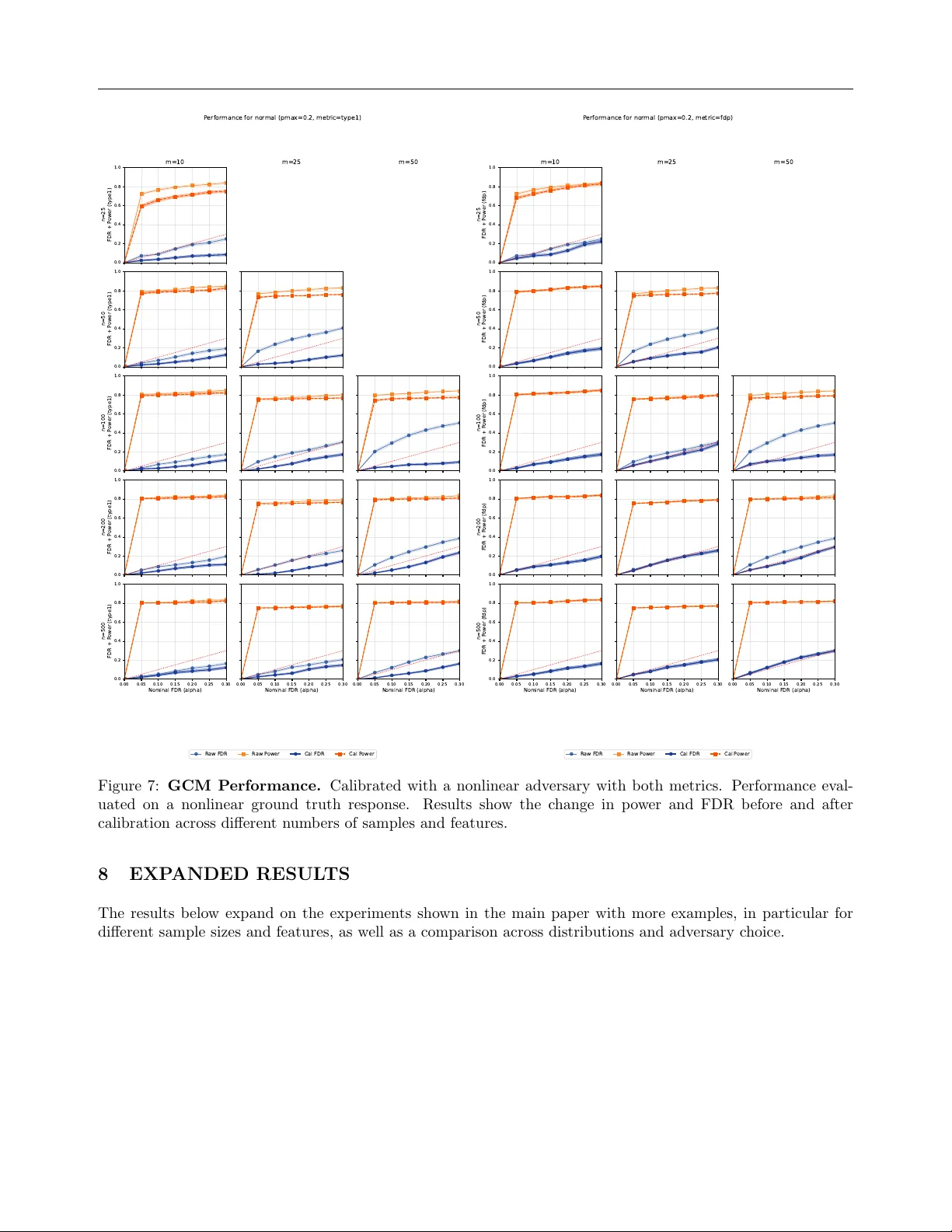
Empirically Calibrated Conditional Indep endence T ests Milleno P an An toine de Mathelin W esley T ansey Computational Oncology Memorial Sloan Kettering Cancer Cen ter Abstract Conditional indep endence tests (CIT) are widely used for causal disco v ery and feature selection. Ev en with false disco v ery rate (FDR) con trol procedures, they often fail to pro vide frequentist guarantees in practice. W e highlight tw o common failure mo des: (i) in small samples, asymptotic guarantees for man y CITs can be inaccurate and ev en cor- rectly sp ecified mo dels fail to estimate the noise levels and control the error, and (ii) when sample sizes are large but mo dels are missp ecified, unaccoun ted dependencies sk ew the test’s behavior and fail to return uni- form p-v alues under the null. W e prop ose Empirically Calibrated Conditional Indep en- dence T ests (ECCIT), a metho d that mea- sures and corrects for miscalibration. F or a chosen base CIT (e.g., GCM, HR T), EC- CIT optimizes an adv ersary that selects fea- tures and resp onse functions to maximize a miscalibration metric. ECCIT then fits a monotone calibration map that adjusts the base-test p-v alues in prop ortion to the observ ed miscalibration. Across empirical b enc hmarks on syn thetic and real data, EC- CIT achiev es v alid FDR with higher p o w er than existing calibration strategies while re- maining test agnostic. Co de is av ailable at h ttps://github.com/tansey-lab/ECCIT. 1 INTR ODUCTION The cen tral to ol for rigorously detecting causal rela- tionships in the presence of confounders is the condi- tional indep endence test. Mathematically , there exists Pro ceedings of the 29 th In ternational Conference on Arti- ficial Intelligence and Statistics (AIST A TS) 2026, T angier, Moro cco. PMLR: V olume 300. Cop yright 2026 by the au- thor(s). a causal edge if t wo v ariables X and Y are dep enden t after controlling for all confounders Z ; th us, the null h yp othesis of no causal effect is one of conditional in - dep endence, H 0 : X ⊥ ⊥ Y | Z . (1) One common use case for conditional indep endence testing is the controlled v ariable selection problem. Giv en data { ( X 1 , X 2 , . . . , X m , Y ) i } n i =1 , w e wish to find the set of v ariables S ⊆ [ m ] such that X j ⊥ ⊥ Y | X − j if and only if j ∈ S . That is, we wan t the Marko v blank et of Y . If there are no laten t confounders and all X j v ariables are known not to b e caused by Y (e.g. if eac h X j w as observ ed before Y ), then S corresp onds to the set of causal features of Y . In real world settings with finite data and noisy obser- v ations, it is imp ossible to infer S without some error rate. Here, we w ork within the frequentist hypothe- sis testing framework: the user supplies the pro cedure with an acceptable error rate α and the pro cedure re- turns a candidate set ˆ S . V alid testing pro cedures pro- vide a guarantee that the expected error on ˆ S will be no larger than α , the user-sp ecified threshold. After con trolling the error rate, pro cedures can b e compared based on whether one has a higher true positive rate, also kno wn as p o wer. Statistical metho ds for testing eq. (1) face a challeng- ing task. Theoretically , it is impossible to produce a metho d capable of ha ving non-trivial p o w er against all p ossible alternative hypotheses (Shah and P eters, 2020). Empirically , many metho ds struggle to control the error rate when the n umber of features m is large relativ e to the sample size n . Nonparametric meth- o ds con v erge to o slowly to pro duce v alid frequen tist p -v alues. P arametric assumptions on the structure of the p ossible conditional dependencies improv es sam- ple efficiency , but open one up to mo del missp ecifi- cation. Addressing the issue of error rate con trol in the high-dimensional and low-sample regimes remains an op en problem, motiv ating a growing literature on differen t approaches (T ansey et al., 2021a; Sudarshan et al., 2021; Li and Liu, 2023). Empirically Calibrated Conditional Indep endence T ests The imp ortance of the problem is highlighted b y the gro wing popularity of conditional indep endence tests in science. CITs ha ve been applied to a wide array of biology and medical data (Shen et al., 2019; Bates et al., 2020; T ansey et al., 2021b; Barry et al., 2021; Sudarshan et al., 2020; Niu et al., 2024b) and used in developmen t of mo dels that ha v e b een integrated in to electronic health records (Ra za vian et al., 2020). The ground truth error rate of these pro cedures is un- kno wable, but it is common for scientific datasets to fall into the high-dimensional or lo w-sample regimes where curren t CIT pro cedures typically fail. In this pap er, we prop ose Empircally Calibrated CITs (ECCITs) as a wrapper metho d for a broad class of conditional independence testing pro cedures. ECC- ITs take an existing conditional indep endence testing or controlled v ariable selection pro cedure, paired with a dataset on which a user wishes to apply it. The empirical calibration metho d then optimizes an adv er- sarial mo del to maximally inflate the error rate of the CIT pro cedure on the target dataset. The p -v alues from the CIT pro cedure applied to the dataset are then calibrated such that they would be v alid p -v alues ev en against the adversary . Since ECCITs calibrate against a w orst-case function in a class F , the result- ing procedure is calibrated or conserv ative for all other functions in F . W e explore several design choices inv olv ed in ECCITs and ev aluate their tradeoffs in extensiv e benchmarks. W e ev aluate tw o differen t types of conditional indep en- dence testing pro cedures, conditional randomization tests and the generalized co v ariance metric. W e con- sider tw o different optimization metrics for the adv er- sary and how each choice affects p o wer. W e also ev al- uate sev eral possible function classes for the predic- tiv e mo dels used in our uncalibrated CITs, the ground truth function class generating Y from X , and the ad- v ersary function class against whic h w e are calibrat- ing. In semi-synthetic exp erimen ts on a large gene expression dataset, ECCITs outperform a state-of-the- art metho d for improving robustness of CITs. 2 BA CKGR OUND Disco vering causal relationships equates statistically to discov e ring conditioning sets that render v ari- ables indep endent. Man y metho ds exist for disco v- ering causal relationships using conditional indepen- dence tests (e.g. Spirtes et al., 2000; Kalisch and B ¨ uhlman, 2007; Pellet and Elisseeff, 2008; Kalisch and B ¨ uhlmann, 2008; Strobl et al., 2016). Kim et al. (2021) divide conditional independence testing metho dology in to three groups: lo cal permutations, model-X, and asymptotics. Lo cal permutation metho ds (Margari- tis, 2005; Doran et al., 2014; Sen et al., 2017; Kim et al., 2021) divide the effect v ariable in to sub classes and test by p erm uting within each subclass. Sub class- ing requires either multiple observ ations of the same confounders or some smo othness assumptions. How- ev er, in the case of con tinuous v ariables, ev ery observ a- tion is almost surely going to b e unique. Alternativ ely , smo othness assumptions (e.g. fixed-width binning as in Kim et al. (2021)) can b e leveraged in combination with k ernel-based metho ds (F ukumizu et al., 2007) and metrics like maximum mean discrepancy (Gret- ton et al., 2012). Unfortunately , k ernel metho ds are lik ely to b e underp o w ered in the high-dimensional set- ting as all samples are going to b e far aw ay from each other unless they lie in a lo w-dimensional subspace. Asymptotic metho ds derive a limiting distribution for a particular test statistic. Classical asymptotic meth- o ds (Su and White, 2008; Huang, 2010) require linear or quadratic parametric forms for the causal relation- ships. More recent work has focused on flexible models either via k ernel-based tests (Zhang et al., 2011; W ang et al., 2015; Strobl et al., 2019) or through using black b o x mac hine learning metho ds (Shah and P eters, 2020; Zhou et al., 2020; Sudarshan et al., 2023). Black b ox metho ds t ypically work b y estimating E [ X | Z ] and E [ Y | Z ], then testing the marginal correlation of the residuals of X and Y after subtracting their predicted conditional means. These metho ds hav e the benefit of b eing rate doubly robust: if either the mo del for E [ X | Z ] or the mo del for E [ Y | Z ] is correctly sp ec- ified, and the fitted regressions conv erge sufficien tly fast, then the method will asymptotically control the t yp e I error rate. How ever, in finite samples or with missp ecified mo dels, these metho ds pro vide no theo- retical guaran tees and often fail to con trol the t yp e I error rate, and in practice, it is unknow able whether w e are ever in that regime using black b o x methods. Mo del-X metho ds (Candes et al., 2018) make no as- sumptions ab out the relationship b et ween X and Y. Rather, approaches lik e kno c koffs and conditional ran- domization tests (CR Ts) assume access to a large un- lab eled dataset on whic h to build an accurate mo del of confounders, in particular modeling P ( X | Z ). Such datasets are often a v ailable in scientific domains. F or example, large genomic (Cheng et al., 2015), transcrip- tomic (Garnett et al., 2012; W einstein et al., 2013), and epigenomic (Drost and Clevers, 2018) tumor, cell line, and organoid databases are a v ailable for analysis in biology . Some model-X methods also enjo y the dou- bly robust property asymptotically (Niu et al., 2024a). In finite samples and high dimensions, accurate esti- mation of the conditional distributions is c hallenging. As with doubly robust asymptotic metho ds, mo del-X metho ds often fail to control type I error in practice. Milleno Pan, An toine de Mathelin, W esley T ansey A n umber of metho ds hav e b een prop osed to increase the practical robustness of b oth doubly robust asymp- totic and mo del-X methods. The Corrected P earson Chi-squared CR T (Xu et al., 2024) adapts CR Ts to b e robust to co v ariate shift in the data. The Maxwa y CR T (Li and Liu, 2023) mo dels b oth P ( X | Z ) and P ( Y | Z ), gaining theoretical and practical adv antages o ver a basic CR T that only mo dels the X conditional distribution. Zhang et al. (2025) follow a similar strat- egy b y using generativ e neural net work mo dels to es- timate both conditional distributions. Perhaps most relev ant to this paper, CONTRA (Sudarshan et al., 2021) uses a mixture of real X data and samples from the estimated P ( X | Z ) to train a predictive mo del of Y used to p erform a CR T. By mixing real and syn- thetic data, the predictive mo del is trained to predict using a more realistic v ersion of the co v ariates that will b e sampled in practice, thereby reducing the o ver- all type I error rate. While the ab o ve metho ds all help reduce the o verall t yp e I error or false disco very rate (FDR) inflation in CITs with finite samples, none of them aim to pro duce properly calibrated CITs. The gap to-date is therefore that conducting CITs is some- what robust using these methods, but it is unclear in practice ho w to calibrate a CIT to control the target error rate in finite samples. 3 METHOD Consider a dataset D with m features ( X 1 , . . . , X m ) and a response v ariable Y . The goal is to conduct con- trolled v ariable selection via conditional indep endence tests of the form X j ⊥ ⊥ Y | X − j for j = 1 , . . . , m . Assume for now that a conditional indep endence test- ing procedure T has b een giv en; we will consider tw o concrete examples later. The requirements on T are only that it returns p -v alues for eac h feature. The issue w e wish to resolv e is that in practice it may b e imp ossible to kno w if T will truly return v alid p -v alues, i.e., Uniform(0 , 1) under the n ull h yp othesis. This may b e due to small sample sizes, large feature counts, or mo del missp ecification within T . Any , none, or all of these issues may be present, but we will be agnostic to the v alidit y of the test and, if it is in v alid, the underly- ing cause. Fix suc h a test T that, given ( X , Y ), returns p -v alues w e wish to calibrate. F or an adv ersary class F of resp onse generators Y = f ( X, ϵ ) and a calibra- tion metric M ( · , α ) with target level α , w e define the adv ersary b y Eq. (2), choosing the generator within F that makes the c hosen metric as large as p ossible, yielding the w orst-case miscalibration for T relativ e to the population distribution of X . The exp ectation is ov er the distribution of X ; since this distribution is not necessarily known in practice, we approximate it b y b o otstrap resampling of the observed X . Op- Algorithm 1 Empirical calibration (adversarial ap- proac h). Input: Dataset ( X, Y ); test T : ( X , Y ) 7→ ( p 1 , . . . , p m ); adv ersary class F with f ∈ F and ˜ Y = f ( X, ε ); calibra- tion metric M ( · , α ). Fit the worst-case adversary f ⋆ as in Equation (2). Let H 0 = { j : γ j = 0 } denote the null features under f ⋆ . for b = 1 , . . . , B do Bo otstrap X ( b ) b y resampling rows of X . Sample ˜ Y ( b ) = f ⋆ ( X ( b ) , ε ). Compute p ( b ) = T ( X ( b ) , ˜ Y ( b ) ). end for Construct Cal α from { ( p ( b ) , H ( b ) 0 ) } B b =1 for M ( · , α ). Return the calibrated p-v alues: p cal = Cal α ( T ( X, Y )). timizing the b o otstrap estimate pro duces an empiri- cal optimizer f ∗ and an asso ciated worst-case metric M  T ( X , f ∗ ( X, ϵ )) , α  . A t a high-lev el, our proposed empirical calibration metho d p erforms the f ollowing steps. 1. An adversarial model (chosen from some class F ) is optimized to maximize the miscalibration of the test statistics under a giv en calibration metric M . This mo del is then used to generate adv ersarial outcomes ˜ Y . 2. The test T is applied to ˜ Y to pro duce adv ersarial p -v alues alongside γ , a vector indicating which of the h yp othesis tests should b e rejected. 3. A monotonic map, which w e call the calibrator, is fit to the adv ersarial p -v alues so that the miscalibra- tion under M is prop erly controlled. This map is then applied to the p-v alues generated by the test T on the real data Y . If F and M together capture the desired form of error rate con trol, then b y calibrating against the w orst-case adv ersary , the ab o ve will yield p -v alues that are either prop erly calibrated or conserv ative. Algorithm 1 details the full algorithm in generality . W e next detail specific design c hoices and discuss their motiv ations and impacts. 3.1 Adv ersary optimization Giv en X and a testing procedure T ( X , Y ) that re- turns p -v alues p 1 , . . . , p m . Let F be a class of data- generating mec hanisms for the resp onse Y , written Y = f ( X, ε ) with f ∈ F and noise. Given a cali- bration metric M and target error rate level α , the ECCIT adv ersary chooses f ⋆ ∈ arg max f ∈F E X  M  T ( X , f ( X , ε )) , α  , (2) Empirically Calibrated Conditional Indep endence T ests inflating the calibration metric as muc h as possible within the b ounds of the adversarial class and the data distribution X . Intuitiv ely , a well calibrated test should b e robust against an y p oten tial resp onse, so we w ant to lo ok for the w orst case scenario to calibrate against. Equation (2) requires access to the p opulation distri- bution ov er X . This is to prev en t flexible adversaries from finding edge cases in a single fixed dataset. In practice, w e t ypically do not ha ve access to this sam- pling distribution. Instead, we generate an appro xi- mate exp ectation using the b ootstrap. The adv ersary sp ecifies t wo sets of parameters. The first set is a binary vector γ corresp onding to whic h features X j will b e used to generate the syn thetic Y ( γ j = 1) and which will b e null v ariables ( γ j = 0). The second set is the parameters θ to the function from the non-n ull features to the synthetic Y . F or simplicity , w e mo del the resp onse as an additiv e errors mo del in practice, though the choice is flexible. Specifically , let ˜ Y b e the adv ersarial resp onse such that, ˜ Y = µ θ  X · γ  + ε, ε ∼ P ( ε ) , E [ ε ] = 0 , where µ θ is a mean function with learnable w eights. Our implementation is flexible to the choice of classes of µ θ , so long as it is a smo oth, differentiable func- tion. Learning γ is a non-smo oth problem as it is a discrete vector. W e use the Gumbel-softmax (Jang et al., 2016) to get approximate gradien ts for the bi- nary mask. Both θ and γ are fit jointly . 3.2 Base Conditional Indep endence T est The choice of which uncalibrated conditional indep en- dence testing procedure to use is up to the user. In scenarios where there are large, unlab eled data, it ma y b e more useful to use a mo del-X method. In areas where higher order momen ts are difficult to ap- pro ximate, doubly robust metho ds are more likely to ha ve higher pow er. W e consider one method from eac h class. Generalized Co v ariance Measure (GCM) (Shah and P eters, 2020) Fix j and set Z := X − j . W e fit estimators for the conditional mean ˆ f j ( Z ) ≈ E [ X j | Z ] , ˆ g ( Z ) ≈ E [ Y | Z ] , then form residuals R ( j ) X = X j − ˆ f j ( Z ) , R ( j ) Y = Y − ˆ g ( Z ) , and elemen twise pro ducts R ( j ) = R ( j ) X ⊙ R ( j ) Y . Let ¯ R ( j ) = 1 n P n i =1 R ( j ) i and s 2 ( j ) = 1 n P n i =1 ( R ( j ) i − ¯ R ( j ) ) 2 . The statistic T j = √ n ¯ R ( j ) s ( j ) is appro ximately N (0 , 1), yielding tw o-sided p -v alues p j = 2 { 1 − Φ( | T j | ) } . When the GCM is well-specified, it is rate doubly robust: under the null, the test statis- tic has the correct limiting distribution when the fit- ted regressions for X j | Z and Y | Z con verge sufficiently fast. In finite samples or with misspecification of the conditional exp ectations, it may inflate the error rate. Holdout Randomization T est (HR T) (T ansey et al., 2021a) Let Z := X − j . Under the n ull h y- p othesis, replacing X j b y fresh dra ws from its condi- tional distribution given Z should not worsen predic- tion of Y . The HR T uses held out prediction error as its test statistic. The HR T fits a predictor ˆ h ( · ) of Y from X on a training split, and computes the held out loss on a holdout set I , L obs = 1 |I | X i ∈I ℓ  Y i , ˆ h ( X i )  . As a mo del-X metho d, the HR T estimates the con- ditional distribution ˆ q j ( · | Z ) for X j | X − j . F or b = 1 , . . . , B the HR T draws ˜ X ( b ) j,i ∼ ˆ q j ( · | Z i ) , i ∈ { 1 , . . . , n } , forms ˜ X ( b ) b y replacing column j on the holdout set, and computes randomized losses L ( b ) = 1 |I | X i ∈I ℓ  Y i , ˆ h ( ˜ X ( b ) i )  . Compute L obs and { L ( b ) } B b =1 p er feature. A righ t–tailed p –v alue is then p j = 1 + P B b =1 1 { L ( b ) ≥ L obs } B + 1 . F or computational efficiency , we approximate the n ull distribution of L ( b ) b y a normal distribution using the sample mean and standard deviation of { L ( b ) } and compute p -v alues from this approximation. The train-test split HR T yields v alid p -v alues pro vided ˆ q j is w ell sp ecified and well estimated. 3.3 Calibration Metric Let H 0 ⊆ { 1 , . . . , m } denote the indices of null h y- p otheses, let m 0 = |H 0 | , and let ˆ S ⊆ { 1 , . . . , m } de- note the set of rejected h yp otheses. The choice of met- ric to optimize against directly relates to the particular c hoice of error rate one is trying to control. Milleno Pan, An toine de Mathelin, W esley T ansey In the strictest case, one may wish to target the fami- lywise error rate (FWER), i.e., FWER = P  | ˆ S ∩ H 0 | ≥ 1  , whic h is the multiple-testing analogue of type-I error. W e consider t w o metrics. The first directly measures the realized t yp e-I error. The second calibrates for the target FDR threshold. T yp e-I. Define the empirical CDF of the null p - v alues by b F 0 ( u ) = 1 m 0 X i ∈H 0 1 { p i ≤ u } . Fix a cutoff α ∈ (0 , 1]. Under p erfect calibration the n ull p -v alues are uniform, so the realized t yp e-I error at lev el α is b F 0 ( α ) . W e measure miscalibration by the deviation from the nominal lev el, T ( α ) = b F 0 ( α ) − α. Zero indicates exact calibration and positive v alues in- dicate inflated t yp e-I error. Con trolling FWER is often to o burdensome in large- scale testing because it requires protecting against ev en a single false rejection, whic h typically leads to v ery conserv ative thresholds and substantial loss of p o wer. Instead, a more common target is the false dis- co very rate (FDR), whic h con trols the expected frac- tion of false disco veries among all rejections, FDR = E " | ˆ S ∩ H 0 | | ˆ S | ∨ 1 # . T o calibrate for FDR control with BH, w e use the false disco very proportion (FDP) as the miscalibration score. FDP . A t a target FDR level α , let p (1) ≤ · · · ≤ p ( m ) and define t BH = max n αi m : p ( i ) ≤ αi m o . Reject all p i ≤ t BH . This is the Benjamini-Hoch b erg (BH) algorithm (Benjamini and Ho ch b erg, 1995). Let R = # { i : p i ≤ t BH } and V = # { i ∈ H 0 : p i ≤ t BH } . The miscalibration score is the false discov ery prop ortion (FDP), FDP = V R ∨ 1 . Lo wer v alues indicate b etter calibration with resp ect to BH at lev el α . 3.4 Calibration Giv en the adversary’s worst-case metric, we construct a c alibr ator , a fixed monotone map that turns ra w out- puts in to conserv ative, well-calibrated ones. Fix a calibration metric M , and let φ M ( α ) denote the corresp onding adversarial metric v alue at nominal lev el α . Define the adjusted level as α cal = sup  t ∈ [0 , 1] : φ M ( t ) ≤ α  . That is, we choose the largest nominal lev el whose realized metric under the adversary does not exceed the target α . 3.5 V alidit y Guaran tees The calibrator ab ov e is constructed from the worst- case adv e rsarial v alue of a c hosen metric o v er a fixed class of generators. As a result, calibrating to the w orst case yields v alid or conserv ativ e behavior for an y other generator in the same class. W e formalize this b elo w for the FDP metric, and pro vide the full proof in the supplemen t. Theorem 1. Assume the true c onditional law Y | X lies in the adversary class use d to c ompute the FDP metric function φ FDP ( · ) . Then running BH at level α cal satisfies FDR  BH( α cal )  ≤ α. Mor e over, α cal ≤ α , so the adjustment is c onservative whenever φ FDP ( α ) > α . 4 RESUL TS W e conduct a series of be nc hmarks to assess calibra- tion and pow er for b oth uncalibrated and ECCIT- calibrated v ersions of GCM and HR T. W e train and calibrate using either Type-I or FDP miscalibration metrics, and ev aluate whether ECCIT calibration can restore uniform p-v alue distributions and control false disco very rates across differen t sources of miscalibra- tion: (i) small sample sizes under a w ell-sp ecified mo del, (ii) under-sp ecification of exogenous noise when the true noise distribution is heavier-tailed, and (iii) mo del under-sp ecification when the conditional esti- mators and ground truth conditionals mismatc h. In our exp eriments, we compare ra w (uncalibrated) p -v alues to FDP and T yp e-I calibrated v ariants, ev al- uating p o wer and realized FDR at α = 0 . 2, a stan- dard fixed target level. On synthetic data, calibra- tion reduces finite-sample miscalibration. The FDP calibration metric t ypically preserves more nominal disco veries, while the Type-I metric enforces worst- case calibration at the level of each individual test, Empirically Calibrated Conditional Indep endence T ests rather than a veraging error across many hypotheses. This makes the T yp e-I metric inherently more con- serv ative. W e also compare ECCIT-calibrated GCM and HR T against a state-of-the-art robustification metho d, CONTRA (Sudarshan et al., 2021). On semi- syn thetic benchmarks, ECCIT-calibrated GCM and HR T outp erform CONTRA-calibrated v ersions, par- ticularly under noise or mo del under-sp ecification. 4.1 Syn thetic Data Exp erimen ts T o test calibration when conditional models are harder to estimate—e.g., under heavy tails, non-Gaussian noise, or cross-feature dep endence—we ev aluate sev- eral feature distributions. By default we sample inde- p enden t features, i.e., X ij are i.i.d. with zero mean: • Normal: X ij ∼ N (0 , 1). • Laplace: X ij ∼ Laplace(0 , 1 / √ 2). • Studen t-t: X ij ∼ t 1 . W e also test on correlated data with shared laten t structures. F or our Correlated distribution setup, w e introduce a one–factor structure X = γ z 1 ⊤ + p 1 − γ 2 E , z ∼ N (0 , 1) , E ij ∼ N (0 , 1) , with γ = 0 . 5, yielding pairwise correlation ≈ γ 2 = 0 . 25. W e set n ≥ 2 m in all runs to keep the GCM normal- equation matrices full-rank and well-conditioned, to obtain low-v ariance CDF/FDP maps from b o otstrap resamples, and to retain enough data for testing. Resp onses Y . T o test the performance of our cali- brated test, w e ev aluate t wo resp onse mo dels for Y : a sparse linear mo del and a simple nonlinear mo del. Linear resp onse. W e use a sparse linear mo del with s activ e features (chosen uniformly without replace- men t) and Gaussian noise: Y = X S β S + ε, β S ∼ N (0 , I s ) , ε ∼ N (0 , I n ) . The n um b er of activ e features dep ends on m : we set s = 5 , 8 , 10 active features for m = 10 , 25 , 50, resp ec- tiv ely . Nonlinear resp onse. Let g = ⌊ s/ 4 ⌋ and split the first 4 g selected indices into g blo c ks of four, { i b, 1 , i b, 2 , i b, 3 , i b, 4 } . F or eac h blo c k we add t wo linear terms and one simple nonlinearit y: Y = a g X b =1  w b 1 X i b, 1 + w b 2 X i b, 2  + b g X b =1 u b tanh  c X i b, 3  + a 2 X j ∈ L v j X j + ε. Here w b 1 , w b 2 , u b , v j ∼ N (0 , 1) indep enden tly; a, b, c > 0 are fixed gains; L contains an y remaining selected indices not used in the blo c ks; and ε ∼ N (0 , I n ). Mo del Regressors. W e use t wo estimator families inside the tests and mirror the same c hoices in the adv ersary . Linear (Ridge). F or eac h feature j with Z := X − j , w e fit ˆ f j ( z ) = z ⊤ ˆ β ( x ) j , ˆ g ( z ) = z ⊤ ˆ β ( y ) , where ˆ β ( x ) j = ( Z ⊤ Z + λI ) − 1 Z ⊤ X j , ˆ β ( y ) = ( Z ⊤ Z + λI ) − 1 Z ⊤ Y , with a small ridge λ > 0 for stabilit y . Nonlinear (MLP). W e replace the linear maps by a single–hidden–la yer netw ork with ReLU: h ( z ) = W 2 ReLU( W 1 z + b 1 ) + b 2 , and set ˆ f j ( z ) = h ( x ) j ( z ) , ˆ g ( z ) = h ( y ) ( z ) with separate functions for predicting X j and Y from Z . Adv ersary . The adversarial generator uses the same families to parameterize the conditional mean of Y . P o w er. W e compute p ow er as the fraction of true features reco vered after applying BH correction at level α = 0 . 2. The Type-I metric we use is also set so that p max = 0 . 2. T o rep ort p o wer only when the FDR target is met, we use valid p ower as defined by T osh et al. (2025): vp( α ) =      0 , if FDR( α ) > α, # { rejected true non-n ulls } # { true non-n ulls } , otherwise , where FDR( α ) = [ FDR( α ) − CI FDR is the 95% low er confidence b ound for the a verage observed FDR at lev el α estimated ov er rep eated runs. V alid pow er equals standard p ow er but is set to zero whenev er the FDR constraint is not satisfied. F or all results on test p erformance, we are doing an a v erage ov er 100 runs on a compute cluster, each pro cess using 1 compute no de. 4.2 Single Hyp othesis T esting While our primary emphasis is on the multiple hy- p othesis setting, ECCITs also apply in the single h y- p othesis framework. In particular, the same calibrated Milleno Pan, An toine de Mathelin, W esley T ansey 0.00 0.05 0.10 0.15 0.20 0.25 0.30 Nominal alpha 0.0 0.2 0.4 0.6 0.8 1.0 T ype-I + P ower Single e xperiment perfor mance (cor r elated, HR T) T ype-I raw P ower raw T ype-I calibrated P ower calibrated T ar get T ype-I Figure 1: Single Exp erimen t Performance. Real- ized Type-I error and p o w er versus nominal α for raw and calibrated HR T on a correlated dataset. mapping can b e used to correct finite-sample Type-I error for a single test statistic and target lev el. W e use the same nonlinear response construction. W e first generate X = Z ⊤ β X + ε X , Z ∈ R 10 , n = 200 , then set Y null = a ( w 1 Z i 1 + w 2 Z i 2 ) + b u tanh( Z i 3 ) + ε, Y alt = Y 0 + tanh( X ) . Here we fix a = 2, b = 3, and sample coefficients w 1 , w 2 , u with non-tin y magnitudes |N (0 , 1) | + 1. W e c hose these parameters to strik e a balance betw een mo del complexit y and signal strength, while preserv- ing enough signal for reliable detection. W e ev aluate α ∈ { 0 , 0 . 05 , . . . , 0 . 30 } and rep ort realized Type-I and p o wer b efore/after calibration. F or the indep enden t setting, Z ∼ N (0 , I ); for the correlated setting, Z gets a shared correlation structure Z ij = γ U i + p 1 − γ 2 ε ij with γ = 0 . 5. Figure 1 sho ws significant improv ement in T yp e-I error con trol with a tradeoff in pow er. Ad- ditional results are sho wn in the supplement. 4.3 Sample and F eature Scaling W ell-sp ecified setting. F or our CITs, a wel l sp e c- ifie d test is when the regression class used inside the test can correctly map the true conditionals: there exist functions f j , g in the fitted class such that f j ( x − j ) = E [ X j | X − j = x − j ] and g ( x − j ) = E [ Y | X − j = x − j ], and for n ull features Y ⊥ X j | X − j . In this regime, as n → ∞ the residuals are mean-zero and the induced p -v alues are uniform. Under a well-specified model, miscalibration is driv en primarily by finite-sample noise and fades as n grows. Here we train the calibrator against a linear adversary and fit linear regressors in both GCM and HR T. T o demonstrate this, w e report calibration results across v arying sample sizes and feature counts to sho w how our calibration results are impacted by the dimensions of our data. In this regime, b oth tests exhibit compa- rable calibrated p erformance. In Figure 2, we see that ev en with a well sp ecified mo del, both tests exhibit finite-sample deviation: for smaller n , the residual–pro duct statistic is noisy and the resulting p -v alues depart from uniformity , increas- ingly so as m grows. Our calibration here revolv es around controlling for the sample noise to hav e a cali- brated test. 4.4 Calibration under Mo del Undersp ecification Under-sp ecifed Setting. The test-side regressors can be undersp e cifie d : if the learners for ˆ f j or ˆ g cannot capture the dep endence of Y on X − j , residual struc- ture remains and the resulting p -v alues are biased. T o test this, we train the calibrator against a nonlinear adv ersary while the tests themselves use linear regres- sors, and we ev aluate on data generated from a non- linear resp onse Y . F or each configuration, we fit the calibrator and ev aluate the p erformance for both the uncalibrated and calibrated tests. In Figure 3, the differences b et ween the results for cali- brating with our Type-I metric versus the FDP metric sho w us a calibration and p o wer tradeoff. The T yp e- I calibrator applies a more conserv ative correction on [0 , α ]. In the ground-truth nonlinear setting consid- ered, this stronger correction did not substantially p e- nalize p o wer; ho wev er, in other resp onse regimes the same global correction could o ver-adjust small p -v alues and reduce disco veries. By contrast, the FDP calibra- tor is targeted to BH: it selects the smallest lev el α cal whose realized FDP do es not exceed the target, effec- tiv ely bringing the threshold bac k to the limit. As a result, FDP calibration typically preserves more nom- inal pow er sub ject to the FDR constrain t, whereas our T yp e-I metric tends to b e more conserv ativ e but can pro vide robustness when miscalibration v aries across quan tiles. Again, the Type-I metric calibrates at the lev el of each individual test, and will drive do wn nom- inal p o wer as a result. 4.5 Robustness to Distributions and Noise Laten t structure and heavy–tailed noise in X can de- grade the conditional fits used by the tests, yielding distorted p -v alues. W e set up this exp erimen t to ev al- uate how well calibration restores FDR control and p o wer when w e v ary the feature distribution and noise Empirically Calibrated Conditional Indep endence T ests 25 100 500 Sample size n (log10 scale) 0.0 0.1 0.2 0.3 0.4 0.5 0.6 R ealized T ype-I @ =0.20 nor mal m=10 m=25 m=50 (a) GCM (Type-I) 25 100 500 Sample size n (log10 scale) 0.0 0.1 0.2 0.3 0.4 0.5 0.6 R ealized T ype-I @ =0.20 nor mal m=10 m=25 m=50 (b) HR T (T yp e-I) 25 100 500 Sample size n (log10 scale) 0.0 0.1 0.2 0.3 0.4 0.5 0.6 R ealized FDP @ =0.20 nor mal m=10 m=25 m=50 (c) GCM (FDP) 25 100 500 Sample size n (log10 scale) 0.0 0.1 0.2 0.3 0.4 0.5 0.6 R ealized FDP @ =0.20 nor mal m=10 m=25 m=50 (d) HR T (FDP) Figure 2: Miscalibration o v er sample size (log scaled) by features on a well-specified mo del for b oth miscalibration metrics. The red dotted line indicates the selected nominal threshold of α = 0 . 2. m=10 m=25 m=50 F eatur e Count (m) 0.0 0.1 0.2 0.3 0.4 0.5 0.6 0.7 0.8 V alid P ower Gain V alid P ower Gain by F eatur e Count - Nor mal GCM (T ype-I) GCM (FDP) HR T (T ype-I) HR T (FDP) Figure 3: V alid P ow er Gain b y F eatures. Cali- brated with a nonlinear adversary . Performance ev al- uated with 10 m samples on a nonlinear resp onse Y . family . In this example, we keep the test side using linear regressors in GCM/HR T while training the cali- brator against a nonlinear adversary and ev aluating on data generated from a nonlinear response Y . In Fig- ure 4, w e show that across different distributions and noise, we are able to improv e on the tests and gain v alid p o wer through calibration. 4.6 Comparisons on Gene Expression Data T o illustrate a realistic use case, we apply our condi- tional indep endence tests to v ariable selection in gene cor r elated laplace nor mal Distribution 0.0 0.1 0.2 0.3 0.4 0.5 0.6 0.7 0.8 V alid P ower Gain V alid P ower Gain by Distribution (n=250, m=25) GCM (T ype-I) GCM (FDP) HR T (T ype-I) HR T (FDP) Figure 4: V alid Po wer Gain b y Distribution. Cal- ibrated with a nonlinear adversary . Performance ev al- uated on a nonlinear resp onse Y . expression analysis. This is often used due to the fea- ture space for gene expression data. Gene features are high-dimensional and e xhibit strong cross-gene cor- relation and latent structure, and these raw coun ts are often mo deled with zero-inflated negative binomi- als. W e construct a semi-synthetic b enc hmark from the Genomics of Drug Sensitivity in Cancer (GDSC) dataset Y ang et al. (2013), treating cancer cell lines as samples ( n ) and genes as features ( m ). W e normal- ize the expression matrix, apply a v ariance-stabilizing log transform, and z -score eac h gene. W e then com- Milleno Pan, An toine de Mathelin, W esley T ansey 0.00 0.05 0.10 0.15 0.20 0.25 0.30 Nominal FDR 0.0 0.2 0.4 0.6 0.8 1.0 V alid P ower V alid P ower on GDSC (Nonlinear, GCM) GCM (Uncalibrated) GCM (Calibrated) 0.00 0.05 0.10 0.15 0.20 0.25 0.30 Nominal FDR 0.0 0.2 0.4 0.6 0.8 1.0 V alid P ower V alid P ower on GDSC (Nonlinear, HR T) HR T (Uncalibrated) HR T (Calibrated) CONTR A -HR T CONTR A -F AST CR T 0.00 0.05 0.10 0.15 0.20 0.25 0.30 Nominal FDR 0.0 0.2 0.4 0.6 0.8 1.0 R ealized FDR R ealized FDR on GDSC (Nonlinear, GCM) GCM (Uncalibrated) GCM (Calibrated) T ar get FDR 0.00 0.05 0.10 0.15 0.20 0.25 0.30 Nominal FDR 0.0 0.2 0.4 0.6 0.8 1.0 R ealized FDR R ealized FDR on GDSC (Nonlinear, HR T) HR T (Uncalibrated) HR T (Calibrated) CONTR A -HR T CONTR A -F AST CR T T ar get FDR Figure 5: V alid Po wer and FDR Comparison on Gene Expression Data. Calibrated with FDP metric. Nonlinear resp onse Y . pare uncalibrated and calibrated GCM/HR T against CONTRA baselines under both linear and nonlinear outcome mo dels. F or each replicate, w e draw a 200 × 25 slice, synthesize outcomes under nonlinear responses, run all metho ds with and without calibration, and ag- gregate p o wer/FDR ov er 100 runs. Additional exp eri- men ts and metho d comparisons on other datasets are rep orted in the supplement. Figure 5 shows that calibration restores FDR con trol for b oth GCM and HR T and increases v alid p o w er relativ e to baseline metho ds lik e CONTRA. W e ev alu- ate p erformance b y sw eeping the BH target level ov er α ∈ { 0 , 0 . 05 , . . . , 0 . 30 } and rep orting FDR and pow er at eac h level. The calibrated tests trac k the nominal FDR and deliver consistent gains in v alid p o wer com- pared to our uncalibrated p erformance. The CONTRA-HR T v arian t struggles in our high- dimensional, correlated gene-expression setting: its conditional sampler for X j | X − j is missp ecified and the predictor is not refit under null draws, yield- ing miscalibrated p -v alues and reduced v alid p ow er. CONTRA-F ASTCR T also p erforms p oorly here be- cause it fits only one null model p er feature and reuses a fixed statistic across n ull resamples. Even though these tests pro vide v ery high nominal pow er, they ha ve a high prop ortion of false discov eries that give us very lo w v alid p o w er. 5 DISCUSSION ECCIT is a practical approach for calibrating con- ditional independence tests when nominal guarantees break down in practice. In our exp erimen ts, it im- pro ves calibration and increases v alid p o wer relative to existing correction metho ds while remaining agnos- tic to the base test. A key limitation is the tradeoff b etw een robustness and p o wer. In ECCIT, this tradeoff is driven b y the choice of adversary class, whic h depends on prior knowledge ab out the true underlying resp onse mechanism. If the class is to o simple, it may lead to insufficient correc- tion. If it is to o flexible, the worst-case calibration ma y b ecome ov erly conserv ative and reduce p o wer. A natural extension is to improv e p o wer o ver a set of plausible resp onse mec hanisms. W e lea ve this direc- tion to future w ork. Empirically Calibrated Conditional Indep endence T ests References Timoth y Barry , Xuran W ang, John A Morris, Kathryn Ro eder, and Eugene Katsevic h. SCEPTRE im- pro ves calibration and sensitivity in single-cell CRISPR screen analysis. Genome Biolo gy , 22(1): 1–19, 2021. Stephen Bates, Matteo Sesia, Chiara Sabatti, and Em- man uel Cand ` es. Causal inference in genetic trio studies. Pr o c e e dings of the National A c ademy of Sci- enc es , 117(39):24117–24126, 2020. Y oav Benjamini and Y osef Ho c hberg. Controlling the false discov ery rate: A practical and p ow erful ap- proac h to multiple testing. Journal of the R oyal Statistic al So ciety: Series B (Statistic al Metho dol- o gy) , 57(1):289–300, 1995. Emman uel Candes, Yingying F an, Lucas Janson, and Jinc hi Lv. Panning for gold: ‘mo del-x’ kno c koffs for high dimensional controlled v ariable selection. Journal of the R oyal Statistic al So ciety: Series B (Statistic al Metho dolo gy) , 80(3):551–577, 2018. Dona v an T. Cheng, T alia N. Mitchell, Ahmet Ze- hir, Ronak H. Shah, Ryma Bena yed, Aijazuddin Sy ed, Raghu Chandramohan, Zhen Y u Liu, He- len H. W on, Sasin ya N. Scott, A. Rose Bran- non, Catherine O’Reilly , Just yna Sado wsk a, Jac k- lyn Casanov a, Angela Y annes, Jaclyn F. Hech t- man, Jinjuan Y ao, W ei Song, Dara S. Ross, Alifya Oultac he, Snjezana Dogan, Laetitia Borsu, Meera Hameed, Khedoudja Nafa, Maria E. Arcila, Marc Ladan yi, and Michael F. Berger. Memorial Sloan Kettering-in tegrated mutation profiling of action- able cancer targets (msk-impact): A hybridization capture-based next-generation sequencing clinical assa y for solid tumor molecular oncology . The Jour- nal of Mole cular Diagnostics , 17(3):251–264, 2015. ISSN 1525-1578. doi: https://doi.org/10.1016/j. jmoldx.2014.12.006. Gary Doran, Krik amol Muandet, Kun Zhang, and Bernhard Sc h¨ olk opf. A permutation-based k ernel conditional independence test. In Pr o c e e dings of the Thirtieth Confer enc e on Unc ertainty in Artifi- cial Intel ligenc e , pages 132–141, 2014. Jarno Drost and Hans Clev ers. Organoids in cancer researc h. Natur e R eviews Canc er , 2018. Kenji F ukumizu, Arthur Gretton, Xiaohai Sun, and Bernhard Sc h¨ olk opf. Kernel measures of conditional dep endence. In Pr o c e e dings of the 20th International Confer enc e on Neur al Information Pr o c essing Sys- tems , pages 489–496, 2007. Mathew J. Garnett, Elena J. Edelman, Sonja J. Heidorn, Chris D. Greenman, Anahita Dastur, King W ai Lau, Patricia Greninger, I. Richard Thompson, Xi Luo, Jorge Soares, et al. Systematic iden tification of genomic markers of drug sensitivity in cancer cells. Natur e , 483(7391):570, 2012. Arth ur Gretton, Karsten M Borgwardt, Malte J Rasc h, Bernhard Sch¨ olk opf, and Alexander Smola. A k ernel t wo-sample test. The Journal of Machine L e arning R ese ar ch , 13(1):723–773, 2012. Tzee-Ming Huang. T esting conditional independence using maximal nonlinear conditional correlation. The Annals of Statistics , 38(4):2047–2091, 2010. Eric Jang, Shixiang Gu, and Ben Poole. Categori- cal reparameterization with Gumbel-softmax. arXiv pr eprint arXiv:1611.01144 , 2016. Markus Kalisch and P eter B ¨ uhlman. Estimating high- dimensional directed acyclic graphs with the p c- algorithm. Journal of Machine L e arning R ese ar ch , 8(3), 2007. Markus Kalisch and Peter B ¨ uhlmann. Robustifica- tion of the PC-algorithm for directed acyclic graphs. Journal of Computational and Gr aphic al Statistics , 17(4):773–789, 2008. Ilm un Kim, Matey Neyko v, Siv araman Balakrish- nan, and Larry W asserman. Lo cal p erm utation tests for conditional indep endence. arXiv pr eprint arXiv:2112.11666 , 2021. Sh uangning Li and Molei Liu. Maxw ay CR T: improv- ing the robustness of the mo del-x inference. Journal of the R oyal Statistic al So ciety Series B: Statistic al Metho dolo gy , 85(5):1441–1470, 2023. Dimitris Margaritis. Distribution-free learning of ba yesian net work structure in contin uous domains. In Pr o c e e dings of the 20th National Confer enc e on A rtificial Intel ligenc e , volume 2, pages 825–830, 2005. Ziang Niu, Abhina v Chakrab ort y , Oliver Duk es, and Eugene Katsevich. Reconciling mo del-x and doubly robust approac hes to conditional independence test- ing. The Annals of Statistics , 52(3):895–921, 2024a. Ziang Niu, Jyotishk a Ray Choudhury , and Eugene Katsevic h. Computationally efficien t and statisti- cally accurate conditional indep endence testing with spaCR T. arXiv pr eprint arXiv:2407.08911 , 2024b. Jean-Philipp e Pellet and Andr´ e Elisseeff. Using Mark ov blankets for causal structure learning. Jour- nal of Machine L e arning R ese ar ch , 9(7), 2008. Narges Raza vian, Vincen t J Ma jor, Mukund Sudar- shan, Jesse Burk-Rafel, P eter Stella, Hardev Rand- ha wa, Seda Bilaloglu, Ji Chen, V uthy Nguy , W alter W ang, Hao Zhang, Ilan Reinstein, Da vid Kudlo witz, Camron Zenger, Meng Cao, Ruina Zhang, Siddhant Dogra, Keerthi Harish, Brian Bosworth, F ritz F ran- cois, Leora Horo witz, Ra jesh Ranganath, Jonathan Milleno Pan, An toine de Mathelin, W esley T ansey Austrian5, and Yindalon Aphiny anaphongs. A v ali- dated, real-time prediction mo del for fav orable out- comes in hospitalized covid-19 patients. NPJ digital me dicine , 3(1):1–13, 2020. Ra jat Sen, Ananda Theertha Suresh, Karthikey an Shanm ugam, Alexandres G Dimakis, and Sanjay Shakk ettai. Model-p o wered conditional indepen- dence test. In Pr o c e e dings of the 31st International Confer enc e on Neur al Information Pr o c essing Sys- tems , pages 2955–2965, 2017. Ra jen D Shah and Jonas Peters. The hardness of con- ditional indep endence testing and the generalised co v ariance measure. The Annals of Statistics , 48 (3):1514–1538, 2020. Arlina Shen, Han F u, Kevin He, and Hui Jiang. F alse disco very rate con trol in cancer biomark er selection using kno c koffs. Canc ers , 11(6):744, 2019. P eter Spirtes, Clark N Glymour, Ric hard Scheines, and David Hec kerman. Causation, pr e diction, and se ar ch . MIT press, 2000. Eric V Strobl, Peter L Spirtes, and Sh yam Visw eswaran. Estimating and controlling the false disco very rate for the PC algorithm using edge- sp ecific p-v alues. arXiv pr eprint arXiv:1607.03975 , 2016. Eric V Strobl, Kun Zhang, and Shy am Visw eswaran. Appro ximate kernel-based conditional independence tests for fast non-parametric causal discov ery . Jour- nal of Causal Infer enc e , 7(1), 2019. Liang jun Su and Halbert White. A nonparametric hellinger metric test for conditional indep endence. Ec onometric The ory , 24(4):829–864, 2008. Mukund Sudarshan, W esley T ansey , and Ra jesh Ran- ganath. Deep direct likelihoo d knock offs. In A d- vanc es in Neur al Information Pr o c essing Systems , v olume 33, pages 5036–5046, 2020. Mukund Sudarshan, Aahlad Puli, Lakshmi Subrama- nian, Sriram Sank araraman, and Ra jesh Ranganath. CONTRA: Con trarian statistics for controlled v ari- able selection. In International Confer enc e on A r- tificial Intel ligenc e and Statistics , pages 1900–1908. PMLR, 2021. Mukund Sudarshan, Aahlad Puli, W esley T ansey , and Ra jesh Ranganath. DIET: Conditional indepen- dence testing with marginal dep endence measures of residual information. In International Confer- enc e on A rtificial Intel ligenc e and Statistics , pages 10343–10367. PMLR, 2023. W. T ansey , V. V eitc h, H. Zhang, R. Rabadan, and D. M. Blei. The holdout randomization test for fea- ture selection in blac k b o x mo dels. Journal of Com- putational and Gr aphic al Statistics , 2021a. W esley T ansey , Kathy Li, Haoran Zhang, Scott W. Linderman, Raul Rabadan, David M. Blei, and Chris H. Wiggins. Dose-resp onse mo deling in high- throughput cancer drug screenings: An end-to-end approac h. Biostatistics , 2021b. PMC Journal - In Pro cess. Curtis T osh, Bo w en Zhang, and W esley T ansey . T reat- men t resp onse as a latent v ariable. arXiv pr eprint arXiv:2502.08776 , 2025. Xueqin W ang, W enliang P an, W enhao Hu, Y uan Tian, and Heping Zhang. Conditional distance correlation. Journal of the Americ an Statistic al Asso ciation , 110 (512):1726–1734, 2015. John N. W einstein, Eric A. Collisson, Gordon B. Mills, Kenna R. Mills Shaw, Brad A. Ozenberger, Kyle Ellrott, Ilya Shm ulevich, Chris Sander, Josh ua M. Stuart, and Cancer Genome Atlas Research Net- w ork. The cancer genome atlas pan-cancer analysis pro ject. Natur e Genetics , 45(10):1113, 2013. Bo wen Xu, Yiwen Huang, Chuan Hong, Shuangn- ing Li, and Molei Liu. Cov ariate shift corrected conditional randomization test. In A. Glob erson, L. Mack ey , D. Belgrav e, A. F an, U. Paquet, J. T om- czak, and C. Zhang, editors, A dvanc es in Neur al Information Pr o c essing Systems , volume 37, pages 78027–78052. Curran Asso ciates, Inc., 2024. W anjuan Y ang, Jorge Soares, P atricia Greninger, Elena J. Edelman, How ard Ligh tfo ot, Sally F orb es, Nishan t Bindal, David Beare, John A. Smith, Ian R. Thompson, Sridhar Ramaswam y , P . An- drew F utreal, Daniel A. Haber, Michael R. Stratton, Cyril H. Benes, Ultan McDermott, and Mathew J. Garnett. Genomics of drug sensitivit y in cancer (gdsc): a resource for therap eutic biomarker discov- ery in cancer cells. Nucleic A cids R ese ar ch , 41(D1): D955–D961, 2013. doi: 10.1093/nar/gks1111. Kun Zhang, Jonas Peters, Dominik Janzing, and Bern- hard Sch¨ olkopf. Kernel-based conditional indepen- dence test and application in causal discov ery . In Pr o c e e dings of the Twenty-Seventh Confer enc e on Unc ertainty in Artificial Intel ligenc e , pages 804– 813, 2011. Yi Zhang, Linjun Huang, Y un Y ang, and Xiaofeng Shao. Doubly robust conditional independence test- ing with generativ e neural net w orks. Journal of the R oyal Statistic al So ciety Series B: Statistic al Metho dolo gy , page qk af047, 2025. Y eqing Zhou, Jingyuan Liu, and Liping Zhu. T est for conditional indep endence with application to condi- tional screening. Journal of Multivariate A nalysis , 175:104557, 2020. Empirically Calibrated Conditional Indep endence T ests Supplemen tary Materials 6 PR OOF This is a detailed pro of of Theorem 1 in the pap er related to v alidity guarantees. 6.1 Hyp othesis testing. Fix a nominal alpha level α ∈ (0 , 1) and a multiple testing pro cedure T α whic h, giv en data ( X , Y ), returns a rejection set T α : ( X, Y ) 7→ R α ( X, Y ) ⊆ H , where H is the index set of h yp otheses. In the main pap er, the sp ecific c hoice is T α = BH( α ), but we write the pro of for a generic multiple testing pro cedure T α . Let V α ( X, Y ) denote the n umber of false rejections among R α ( X, Y ) under the true data generating pro cess. W e then define the false disco very prop ortion as FDP α ( X, Y ) := V α ( X, Y ) max {| R α ( X, Y ) | , 1 } . The corresp onding false discov ery rate (FDR) at level α is: FDR α := E  FDP α ( X, Y )  . 6.2 FDP loss. W e first define the p oin t wise FDP loss at level α : ℓ α ( Y ) :=  FDP α ( X, Y ) − α  + = max { FDP α ( X, Y ) − α , 0 } , so that ℓ α ( Y ) = 0 whenever FDP α ( X, Y ) ≤ α , and ℓ α ( Y ) measures the amount by which w e exceed lev el α otherwise. 6.3 Adv ersarial mo del and miscalibration. In our calibration procedure, we consider a class of adv ersary functions F (for example, linear maps f : R p → R ). F or eac h f ∈ F , the adv ersary specifies a conditional distribution P f ( Y | X ) (e.g., Y = f ( X ) + ε with a fixed noise mo del). W e write Y f ∼ P f ( · | X ) for a random outcome generated under this adversarial mo del. W e then define the miscalibration of f at nominal level α as L α ( f ) := E  ℓ α ( Y f )  = E  (FDP α ( X, Y f ) − α ) +  . The ideal adv ersarial ob jective ov er this class is the w orst case miscalibration M F := sup f ∈F L α ( f ) , the largest exp ected excess FDP among all generators f ∈ F . In practice, the adv ersary training only approximately maximizes L α ( f ) ov er f ∈ F . If ˆ f denotes the final adv ersary we obtain, we assume an optimization error ϵ opt suc h that 0 ≤ M F − L α ( ˆ f ) ≤ ϵ opt , Milleno Pan, An toine de Mathelin, W esley T ansey so that L α ( ˆ f ) ≥ M F − ϵ opt , M F ≤ L α ( ˆ f ) + ϵ opt . (3) 6.4 Bounds for a fixed f . F or any fixed f ∈ F and any δ > 0,  FDP α ( X, Y f ) ≥ α + δ  ⊆  FDP α ( X, Y f ) − α  + ≥ δ  , since the even t on the left implies that the excess (FDP α − α ) + is at least δ . Therefore, by Marko v’s inequalit y , P f  FDP α ( X, Y f ) ≥ α + δ  ≤ E  (FDP α ( X, Y f ) − α ) +  δ = L α ( f ) δ . This giv es a tail b ound for the FDP under the adversarial mo del P f . Similarly , the exp ected FDP under P f satisfies E f  FDP α ( X, Y f )  = α + E f  FDP α ( X, Y f ) − α  ≤ α + E f  (FDP α ( X, Y f ) − α ) +  = α + L α ( f ) , so L α ( f ) also controls the FDR for the mo del P f as an excess o ver the nominal level α . 6.5 Bounds when the ground truth lies in F . Supp ose no w that the true conditional distribution P true ( Y | X ) b elongs to our adversary class, in the sense that there exists some f true ∈ F such that P true ( · | X ) = P f true ( · | X ) . Let Y true ∼ P true ( · | X ) denote the true response. By construction, Y true and Y f true ha ve the same conditional distribution giv en X , so any b ound that holds under P f true also holds under P true . By definition of suprem um, and combining (3) with f = f true , L α ( f true ) ≤ M F , L α ( f true ) ≤ L α ( ˆ f ) + ϵ opt . (4) Applying the tail b ound ab o v e with f = f true giv es, for any δ > 0, P true  FDP α ( X, Y true ) ≥ α + δ  = P f true  FDP α ( X, Y f true ) ≥ α + δ  ≤ L α ( f true ) δ ≤ L α ( ˆ f ) + ϵ opt δ . Similarly , for the exp ected FDP under the true mo del, E true  FDP α ( X, Y true )  = E f true  FDP α ( X, Y f true )  ≤ α + L α ( f true ) ≤ α + L α ( ˆ f ) + ϵ opt . Th us, under the assumption that the true conditional distribution Y | X lies in our adversary class F , the optimized adversarial ob jective L α ( ˆ f ) provides an upper bound, up to the optimization error ϵ opt , on both the probabilit y of large FDP ranges and on the FDR of our pro cedure. Empirically Calibrated Conditional Indep endence T ests 6.6 Calibration. F or each nominal level α ∈ (0 , 1) we hav e the b ound B ( α ) := α + L α ( ˆ f ) + ϵ opt . T o match the notation in the main text, we may equiv alently write φ FDP ( α ) := B ( α ) . Since L α ( ˆ f ) ≥ 0 and ϵ opt ≥ 0, the calibration curv e B ( α ) is p oin t wise low er b ounded by the iden tit y map, B ( α ) ≥ α for all α ∈ (0 , 1) . Giv en a desired target FDR level q ∈ (0 , 1), define the calibrated nominal level as the largest nominal level whose w orst-case FDR b ound do es not exceed q : α cal ( q ) := sup  t ∈ [0 , 1] : B ( t ) ≤ q  . By construction, B ( α cal ( q )) ≤ q , and therefore E true  FDP α cal ( q ) ( X, Y true )  ≤ B ( α cal ( q )) ≤ q . The calibrated nominal level is alwa ys less than or equal to the target FDR lev el. In particular, this guarantees that the calibration step can only reduce, or leav e unchanged, the effective FDR of the pro cedure under the true data generating pro cess. Milleno Pan, An toine de Mathelin, W esley T ansey 0.00 0.05 0.10 0.15 0.20 0.25 0.30 Nominal alpha 0.0 0.2 0.4 0.6 0.8 1.0 T ype-I + P ower Single e xperiment perfor mance (nor mal, GCM) T ype-I raw P ower raw T ype-I calibrated P ower calibrated T ar get T ype-I 0.00 0.05 0.10 0.15 0.20 0.25 0.30 Nominal alpha 0.0 0.2 0.4 0.6 0.8 1.0 T ype-I + P ower Single e xperiment perfor mance (cor r elated, GCM) T ype-I raw P ower raw T ype-I calibrated P ower calibrated T ar get T ype-I 0.00 0.05 0.10 0.15 0.20 0.25 0.30 Nominal alpha 0.0 0.2 0.4 0.6 0.8 1.0 T ype-I + P ower Single e xperiment perfor mance (nor mal, HR T) T ype-I raw P ower raw T ype-I calibrated P ower calibrated T ar get T ype-I 0.00 0.05 0.10 0.15 0.20 0.25 0.30 Nominal alpha 0.0 0.2 0.4 0.6 0.8 1.0 T ype-I + P ower Single e xperiment perfor mance (cor r elated, HR T) T ype-I raw P ower raw T ype-I calibrated P ower calibrated T ar get T ype-I Figure 6: Single Exp erimen t P erformance. Realized Type-I error and p o wer versus nominal α for raw and calibrated pro cedures in indep enden t and correlated settings. 7 SINGLE EXPERIMENTS Figure 6 sho ws additional results for the indep enden t and correlated Gaussian settings using GCM and HR T. Empirically Calibrated Conditional Indep endence T ests 0.0 0.2 0.4 0.6 0.8 1.0 n=25 FDR + P ower (type1) m=10 m=25 m=50 0.0 0.2 0.4 0.6 0.8 1.0 n=50 FDR + P ower (type1) 0.0 0.2 0.4 0.6 0.8 1.0 n=100 FDR + P ower (type1) 0.0 0.2 0.4 0.6 0.8 1.0 n=200 FDR + P ower (type1) 0.00 0.05 0.10 0.15 0.20 0.25 0.30 Nominal FDR (alpha) 0.0 0.2 0.4 0.6 0.8 1.0 n=500 FDR + P ower (type1) 0.00 0.05 0.10 0.15 0.20 0.25 0.30 Nominal FDR (alpha) 0.00 0.05 0.10 0.15 0.20 0.25 0.30 Nominal FDR (alpha) P erfor mance for nor mal (pmax=0.2, metric=type1) R aw FDR R aw P ower Cal FDR Cal P ower 0.0 0.2 0.4 0.6 0.8 1.0 n=25 FDR + P ower (fdp) m=10 m=25 m=50 0.0 0.2 0.4 0.6 0.8 1.0 n=50 FDR + P ower (fdp) 0.0 0.2 0.4 0.6 0.8 1.0 n=100 FDR + P ower (fdp) 0.0 0.2 0.4 0.6 0.8 1.0 n=200 FDR + P ower (fdp) 0.00 0.05 0.10 0.15 0.20 0.25 0.30 Nominal FDR (alpha) 0.0 0.2 0.4 0.6 0.8 1.0 n=500 FDR + P ower (fdp) 0.00 0.05 0.10 0.15 0.20 0.25 0.30 Nominal FDR (alpha) 0.00 0.05 0.10 0.15 0.20 0.25 0.30 Nominal FDR (alpha) P erfor mance for nor mal (pmax=0.2, metric=fdp) R aw FDR R aw P ower Cal FDR Cal P ower Figure 7: GCM Performance. Calibrated with a nonlinear adv ersary with both metrics. P erformance ev al- uated on a nonlinear ground truth resp onse. Results show the c hange in p ow er and FDR b efore and after calibration across differen t num b ers of samples and features. 8 EXP ANDED RESUL TS The results b elo w expand on the exp eriments sho wn in the main pap er with more examples, in particular for differen t sample sizes and features, as well as a comparison across distributions and adversary choice. Milleno Pan, An toine de Mathelin, W esley T ansey 0.0 0.2 0.4 0.6 0.8 1.0 n=25 FDR + P ower (type1) m=10 m=25 m=50 0.0 0.2 0.4 0.6 0.8 1.0 n=50 FDR + P ower (type1) 0.0 0.2 0.4 0.6 0.8 1.0 n=100 FDR + P ower (type1) 0.0 0.2 0.4 0.6 0.8 1.0 n=200 FDR + P ower (type1) 0.00 0.05 0.10 0.15 0.20 0.25 0.30 Nominal FDR (alpha) 0.0 0.2 0.4 0.6 0.8 1.0 n=500 FDR + P ower (type1) 0.00 0.05 0.10 0.15 0.20 0.25 0.30 Nominal FDR (alpha) 0.00 0.05 0.10 0.15 0.20 0.25 0.30 Nominal FDR (alpha) P erfor mance for nor mal (pmax=0.2, metric=type1) R aw FDR R aw P ower Cal FDR Cal P ower 0.0 0.2 0.4 0.6 0.8 1.0 n=25 FDR + P ower (fdp) m=10 m=25 m=50 0.0 0.2 0.4 0.6 0.8 1.0 n=50 FDR + P ower (fdp) 0.0 0.2 0.4 0.6 0.8 1.0 n=100 FDR + P ower (fdp) 0.0 0.2 0.4 0.6 0.8 1.0 n=200 FDR + P ower (fdp) 0.00 0.05 0.10 0.15 0.20 0.25 0.30 Nominal FDR (alpha) 0.0 0.2 0.4 0.6 0.8 1.0 n=500 FDR + P ower (fdp) 0.00 0.05 0.10 0.15 0.20 0.25 0.30 Nominal FDR (alpha) 0.00 0.05 0.10 0.15 0.20 0.25 0.30 Nominal FDR (alpha) P erfor mance for nor mal (pmax=0.2, metric=fdp) R aw FDR R aw P ower Cal FDR Cal P ower Figure 8: HR T Performance. Calibrated with a nonlinear adversary with both metrics. P erformance ev aluated on a nonlinear ground truth response. Results show the c hange in pow er and FDR before and after calibration across differen t num b ers of samples and features. Empirically Calibrated Conditional Indep endence T ests 0.00 0.05 0.10 0.15 0.20 0.25 0.30 Nominal T ype-I (alpha) 0.0 0.2 0.4 0.6 0.8 1.0 R ealized T ype-I Nonlinear adversary, Nonlinear GCM Nonlinear adversary, Linear GCM Linear adversary, Nonlinear GCM Linear adversary, Linear GCM Nominal vs R ealized T ype-I | dist=cor r elated (a) Correlated (Type-I) 0.00 0.05 0.10 0.15 0.20 0.25 0.30 Nominal T ype-I (alpha) 0.0 0.2 0.4 0.6 0.8 1.0 R ealized T ype-I Linear adversary, Linear GCM Nonlinear adversary, Nonlinear GCM Linear adversary, Nonlinear GCM Nonlinear adversary, Linear GCM Nominal vs R ealized T ype-I | dist=laplace (b) Laplace (Type-I) 0.00 0.05 0.10 0.15 0.20 0.25 0.30 Nominal T ype-I (alpha) 0.0 0.2 0.4 0.6 0.8 1.0 R ealized T ype-I Linear adversary, Nonlinear GCM Nonlinear adversary, Nonlinear GCM Nonlinear adversary, Linear GCM Linear adversary, Linear GCM Nominal vs R ealized T ype-I | dist=nor mal (c) Normal (Type-I) 0.00 0.06 0.12 0.18 0.24 0.30 Nominal FDR (alpha) 0.0 0.2 0.4 0.6 0.8 1.0 R ealized FDP Nonlinear adversary, Linear GCM Linear adversary, Linear GCM Linear adversary, Nonlinear GCM Nonlinear adversary, Nonlinear GCM Nominal vs R ealized FDP | dist=cor r elated (d) Correlated (FDP) 0.00 0.06 0.12 0.18 0.24 0.30 Nominal FDR (alpha) 0.0 0.2 0.4 0.6 0.8 1.0 R ealized FDP Nonlinear adversary, Nonlinear GCM Linear adversary, Linear GCM Linear adversary, Nonlinear GCM Nonlinear adversary, Linear GCM Nominal vs R ealized FDP | dist=laplace (e) Laplace (FDP) 0.00 0.06 0.12 0.18 0.24 0.30 Nominal FDR (alpha) 0.0 0.2 0.4 0.6 0.8 1.0 R ealized FDP Nonlinear adversary, Linear GCM Linear adversary, Linear GCM Linear adversary, Nonlinear GCM Nonlinear adversary, Nonlinear GCM Nominal vs R ealized FDP | dist=nor mal (f ) Normal (FDP) Figure 9: GCM calibration across distributions. Comparisons b etw een different miscalibration com bina- tions on the adv ersary and the test. T yp e-I metric (top) and FDP metric (b ottom). Milleno Pan, An toine de Mathelin, W esley T ansey 0.00 0.05 0.10 0.15 0.20 0.25 0.30 Nominal T ype-I (alpha) 0.0 0.2 0.4 0.6 0.8 1.0 R ealized T ype-I Nonlinear adversary, Linear HR T Nonlinear adversary, Nonlinear HR T Linear adversary, Linear HR T Linear adversary, Nonlinear HR T Nominal vs R ealized T ype-I | dist=cor r elated (a) Correlated (Type-I) 0.00 0.05 0.10 0.15 0.20 0.25 0.30 Nominal T ype-I (alpha) 0.0 0.2 0.4 0.6 0.8 1.0 R ealized T ype-I Linear adversary, Linear HR T Linear adversary, Nonlinear HR T Nonlinear adversary, Linear HR T Nonlinear adversary, Nonlinear HR T Nominal vs R ealized T ype-I | dist=laplace (b) Laplace (Type-I) 0.00 0.05 0.10 0.15 0.20 0.25 0.30 Nominal T ype-I (alpha) 0.0 0.2 0.4 0.6 0.8 1.0 R ealized T ype-I Linear adversary, Linear HR T Nonlinear adversary, Nonlinear HR T Nonlinear adversary, Linear HR T Linear adversary, Nonlinear HR T Nominal vs R ealized T ype-I | dist=nor mal (c) Normal (Type-I) 0.00 0.06 0.12 0.18 0.24 0.30 Nominal FDR (alpha) 0.0 0.2 0.4 0.6 0.8 1.0 R ealized FDP Linear adversary, Nonlinear HR T Linear adversary, Linear HR T Nonlinear adversary, Nonlinear HR T Nonlinear adversary, Linear HR T Nominal vs R ealized FDP | dist=cor r elated (d) Correlated (FDP) 0.00 0.06 0.12 0.18 0.24 0.30 Nominal FDR (alpha) 0.0 0.2 0.4 0.6 0.8 1.0 R ealized FDP Linear adversary, Nonlinear HR T Linear adversary, Linear HR T Nonlinear adversary, Linear HR T Nonlinear adversary, Nonlinear HR T Nominal vs R ealized FDP | dist=laplace (e) Laplace (FDP) 0.00 0.06 0.12 0.18 0.24 0.30 Nominal FDR (alpha) 0.0 0.2 0.4 0.6 0.8 1.0 R ealized FDP Linear adversary, Nonlinear HR T Nonlinear adversary, Nonlinear HR T Linear adversary, Linear HR T Nonlinear adversary, Linear HR T Nominal vs R ealized FDP | dist=nor mal (f ) Normal (FDP) Figure 10: HR T calibration across distributions. Comparisons b et ween differen t miscalibration com bina- tions on the adv ersary and the test. T yp e-I metric (top) and FDP metric (b ottom). Empirically Calibrated Conditional Indep endence T ests T able 1: Breast Cancer Dataset. Entries are v alid p ow er / realized FDR. Metho d α = 0 . 05 α = 0 . 10 α = 0 . 15 α = 0 . 20 GCM 0.165 / 0.086 0.127 / 0.141 0.125 / 0.181 0.145 / 0.227 Calibrated GCM 0.166 / 0.058 0.179 / 0.070 0.177 / 0.075 0.177 / 0.082 HR T 0.109 / 0.220 0.074 / 0.321 0.053 / 0.388 0.057 / 0.444 Calibrated HR T 0.161 / 0.093 0.146 / 0.137 0.137 / 0.159 0.150 / 0.176 CONTRA-HR T 0.010 / 0.489 0.010 / 0.497 0.010 / 0.502 0.027 / 0.520 CONTRA-F ASTCR T 0.012 / 0.539 0.012 / 0.548 0.008 / 0.562 0.017 / 0.572 T able 2: Wine Dataset. Entries are v alid p ow er / realized FDR. Metho d α = 0 . 05 α = 0 . 10 α = 0 . 15 α = 0 . 20 GCM 0.372 / 0.132 0.292 / 0.203 0.255 / 0.244 0.207 / 0.281 Calibrated GCM 0.432 / 0.043 0.407 / 0.085 0.333 / 0.158 0.292 / 0.204 HR T 0.400 / 0.030 0.388 / 0.050 0.370 / 0.076 0.347 / 0.103 Calibrated HR T 0.400 / 0.030 0.388 / 0.050 0.370 / 0.076 0.347 / 0.103 CONTRA-HR T 0.122 / 0.324 0.122 / 0.333 0.092 / 0.375 0.087 / 0.388 CONTRA-F ASTCR T 0.133 / 0.335 0.125 / 0.352 0.068 / 0.405 0.068 / 0.425 9 ADDITIONAL DA T ASETS W e ha ve added more exp eriments on t w o standard real w orld datasets widely used in other studies, the Diagnostic Wisconsin Breast Cancer dataset and the Wine recognition dataset. Both datasets are a v ailable from the UCI Mac hine Learning Rep ository . F or b oth datasets w e use exactly the same construction as in our GDSC gene expression exp erimen ts: we fix the observ ed cov ariates X , select a small subset of “active” features, and generate a nonlinear resp onse from these activ es plus noise. In the breast cancer configuration we tak e n = 300 samples, m = 30 features, and | S active | = 10; in the wine configuration we tak e n = 100, m = 13, and | S active | = 4. Calibration w as done with our FDP metric and shown in T able 1 and T able 2.