Exchangeable Gaussian Processes for Staggered-Adoption Policy Evaluation

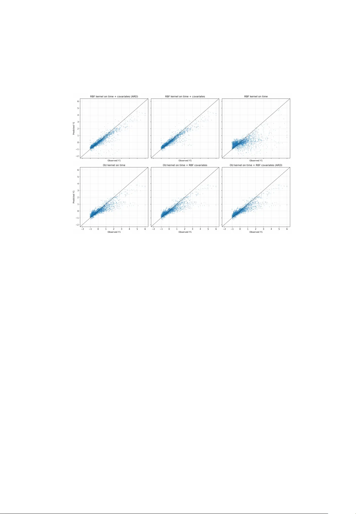
Ex c hang eable Gaussian Processes f or S tagg ered- A doption P olicy Ev aluation Ha yk Ge v orgy an 1 , K onstantinos Kalog eropoulos 2 , and Angelos Ale x opoulos 1 1 Depar tment of Economics, A thens U niv ersity of Economics and Business, A thens, Greece 2 Depar tment of Statis tics, The London School of Economics and P olitical Science, London, United Kingdom F ebr uary 25, 2026 Abstract W e study the use of ex chang eable multi-task Gaussian processes (GPs) f or causal inf erence in panel data, appl ying the framew ork to tw o settings: one with a single treated unit subject to a once-and-for -all treatment and another with multiple treated units and staggered treatment adoption. Our approac h models the joint ev olution of outcomes f or treated and control units through a GP pr ior that ensures e x c hang eability across units while allo wing f or flexible nonlinear trends o v er time. The resulting pos terior predictiv e distribution f or the untreated potential outcomes of the treated unit pro vides a counter f actual path, from which w e der iv e pointwise and cumulativ e treatment effects, along with credible intervals to quantify uncer tainty . W e implement se v eral v ariations of the e xc hang eable GP model using different k ernel functions. T o assess prediction accuracy , we conduct a placebo-style v alidation within the pre-intervention windo w by selecting a “f ak e ” intervention date. Ultimatel y , this s tudy illustrates ho w ex chang eable GPs serve as a fle xible tool f or policy ev aluation in panel data settings and proposes a no vel approach to s tagg ered-adoption designs with a lar ge number of treated and control units. 1 Intr oduction Modern public policy e v aluation increasingly relies on longitudinal datasets that f ollo w multiple units o v er time, such as states, regions, firms or individuals. In man y applications, the central ques tion is to assess the causal effect of a policy inter v ention that affects a subset of units 1 at a kno wn time, using the remaining units as controls to reconstruct the counter factual tra jector y that w ould ha v e been obser v ed, if an intervention ne v er occur red. A prominent frame w ork f or such problems is the synthetic control approach (Abadie and Gardeazabal, 2003; A badie et al., 2010), where the counter factual path of the treated unit is estimated b y a w eighted sum of control units. This and related methods, including f actor -model- based g eneralized synthetic control (X u, 2017) and Ba y esian str uctural time-ser ies models (Brodersen et al., 2015), ha v e been widely applied in economics and public policy . These approaches typicall y rel y on assumptions about the specific functional f orm of the e volution of outcomes o v er time and on linear combinations of control units, which ma y be res trictiv e when trends are nonlinear , co v ar iate effects are complex, or the dynamics differ substantiall y across units. Gaussian process (GP) pr iors (Rasmussen and Williams, 2006) offer a fle xible, non-parametr ic or semi-parametric alter nativ e f or modeling time-ser ies dynamics and co v ariate relationships. The y allo w us to character ize relationships across different units, while remaining unres tricted in functional f or ms. R ecent work has introduced GP -based f or mulations f or counter factual prediction and causal effect estimation in panel data settings (Giudice et al., 2022; Ben-Michael et al., 2022), demonstrating that GPs can pro vide a reliable w ay to quantify uncertainty about the counterfactual path, and they can accommodate nonlinear trends and time-varying relationships. Within the broad class of GPs, exchang eable Gaussian pr ocesses ha v e recently been proposed as a multi-task GP frame work (Lero y et al., 2022; Bouranis et al., 2023) , where a GP prior is placed on the latent mean process shared across units, and each unit-specific deviation is itself a GP , creating an e x changeable str ucture across units. This paper adapts and e xtends the ex chang eable GP frame w ork to the conte xt of causal inf erence with panel data and illustrates its use in tw o applications. The first is the Proposition 99 (Prop99) setting, where units correspond to U .S. states obser v ed annuall y and the treated unit is Calif ornia; the inter v ention associated with Prop99 is introduced f or Calif or nia after 1988, while the remaining states serve as controls. The second dataset is a larg e panel of Greek petrol stations observ ed at w eekl y frequency o v er the course of a y ear . A policy intervention affects a subset of stations at different points in time, while the remaining stations ser v e as ne v er -treated controls. In both settings, our goal is to assess whether the inter v ention had a causal impact on the outcome b y cons tr ucting counterfactual tra jectories f or treated units using the outcomes of non-treated units and co v ariates as predictors. The paper is org anized as f ollo w s. Section 2 introduces the causal inf erence frame w ork, the cor responding assumptions, and a revie w of state-of-the-ar t methods. Section 3 describes the e x chang eable GP model. Section 4 details the model-fitting and inf erence protocol f or stagg ered adoption setting. Section 5 presents the estimation details, including h yperparameter lear ning and the construction of pos ter ior predictiv e counterfactual paths. Section 6 presents the datasets, specifies the empirical design, and repor ts the results of the v alidation and policy -effect anal y ses. 2 2 Causal Inf erence with panel dat a In this section w e f or malize the causal inference problem in a panel time-series setting and introduce the estimands that will be repor ted in the final anal ysis. W e present the potential outcomes frame w ork specific to panel data with a policy inter v ention that affects a single units at a specific point in time. 2.1 P anel structure and potential outcomes Consider a panel with units (e.g., states, fir ms) inde xed b y 𝑖 = 1 , . . . , 𝑚 and discrete time per iods inde x ed b y 𝑡 = 1 , . . . , 𝑇 . Let I = { 1 , . . . , 𝑚 } denote the set of units and T = { 1 , . . . , 𝑇 } the set of time per iods. For each unit and time, w e obser v e an outcome 𝑦 𝑖 𝑡 ∈ R of interest and possibl y a v ector of observ ed co v ariates 𝑥 𝑖 𝑡 ∈ R 𝑝 . A policy inter v ention is introduced at different unit-specific time points, and it affects a subset of units I 1 ⊆ I . The remaining units I 0 = I \ I 1 serve as potential controls. In the remainder of this section, we f ocus on the case of a sing le tr eated unit with a sharp interv ention at time 𝑇 0 , which cor responds to the setting of our empir ical application with a single treated unit (Calif or nia) and is also a simplification f or our applied case of Greek businesses with staggered treatment adoption. Let 𝑖 ★ denote the treated unit, so that I 1 = { 𝑖 ★ } and I 0 contains all other units. W e partition the time axis into a pre-inter v ention per iod T 0 = { 1 , . . . , 𝑇 0 } and a post-inter v ention per iod T 1 = { 𝑇 0 + 1 , . . . , 𝑇 } . For each unit 𝑖 and time 𝑡 , define a treatment indicator 𝑤 𝑖 𝑡 ∈ { 0 , 1 } , where 𝑤 𝑖 𝑡 = 1 if the policy has already been applied to unit 𝑖 at time 𝑡 , and 𝑤 𝑖 𝑡 = 0 otherwise. In the case of a single treated unit with a single strict inter v ention time w e ha v e 𝑤 𝑖 𝑡 = 0 f or all 𝑖 ≠ 𝑖 ★ and 𝑡 , and 𝑤 𝑖 ★ 𝑡 =        0 , 𝑡 ≤ 𝑇 0 , 1 , 𝑡 > 𝑇 0 . Within the potential outcomes frame w ork, f or each ( 𝑖 , 𝑡 ) there are tw o potential outcomes: 𝑦 𝑖 𝑡 ( 0 ) denotes the outcome that w ould be obser v ed f or unit 𝑖 at time 𝑡 in the absence of treatment, and 𝑦 𝑖 𝑡 ( 1 ) denotes the outcome that w ould be obser v ed under treatment. The actual outcome is 𝑦 𝑖 𝑡 = 𝑦 𝑖 𝑡 ( 0 ) I { 𝑤 𝑖 𝑡 = 0 } + 𝑦 𝑖 𝑡 ( 1 ) I { 𝑤 𝑖 𝑡 = 1 } , where I { · } is an indicator function. The fundamental problem is that f or the treated unit 𝑖 ★ , w e onl y observe 𝑦 𝑖 ★ 𝑡 ( 1 ) , and not 𝑦 𝑖 ★ 𝑡 ( 0 ) f or any giv en 𝑡 > 𝑇 0 . Hence, our main task is to es timate the sequence { 𝑦 𝑖 ★ 𝑡 ( 0 ) : 𝑡 ∈ T 1 } , which yields the counter factual path f or the treated unit. 3 2.2 Causal estimands Our pr imary objective is to quantify the causal effect of the policy on the outcome of the treated unit o v er time, together with the uncer tainty around these effects. For each unit 𝑖 , the individual causal effect at time 𝑡 is denoted as 𝛿 𝑖 ,𝑡 = 𝑦 𝑖 ,𝑡 ( 1 ) − 𝑦 𝑖 ,𝑡 ( 0 ) . In our empirical applications, w e consider both the Proposition 99 (Prop99) setting with a single treated unit 𝑖 ★ (Calif ornia) and a Greek business-le v el panel with multiple treated units. In the Prop99 application, we aim to estimate 𝛿 𝑖 ★ ,𝑡 f or all post-intervention times 𝑡 ∈ T 1 = { 𝑇 0 + 1 , . . . , 𝑇 } . In the Greek business application, we are interes ted in estimating 𝛿 𝑖 ,𝑡 f or all treated units 𝑖 ∈ I 1 at all post-interv ention times. Denote the set of outcomes and co variates that are not affected b y the treatment as D 0 . This includes the co v ariates of all units, including the treated unit, and the set of outcomes of untreated units, plus the set of pre-treatment outcomes of the treated unit. Giv en D 0 , w e define the mean of the individual causal effect at time 𝑡 as 𝜏 𝑖 ★ ,𝑡 = E  𝛿 𝑖 ★ ,𝑡 | D 0  , 𝑡 ∈ T 1 . (1) W e are also interested in the uncer tainty sur rounding the causal effect. This can be quantified via the posterior variance 𝜎 2 𝑖 ★ ,𝑡 = V  𝛿 𝑖 ★ ,𝑡 | D 0  , (2) or , eq uiv alentl y , through posterior quantiles 𝑞 𝛿 𝑖 ★ , 𝑡 ( 𝛼 ) = 𝐹 − 1 𝛿 𝑖 ★ , 𝑡  𝛼 | D 0  , 𝛼 ∈ ( 0 , 1 ) , (3) where 𝐹 𝛿 𝑖 ★ , 𝑡 is the posterior cumulativ e distribution function of 𝛿 𝑖 ★ ,𝑡 . W e generall y report central 95% credible inter v als tog ether with the posterior mean 𝜏 𝑖 ★ ,𝑡 f or eac h 𝑡 . Within a Gaussian process frame w ork with Gaussian likelihood, these quantities are straight- f orward to der iv e. The posterior predictiv e distr ibution of the counter factual outcome 𝑦 𝑖 ★ ,𝑡 ( 0 ) giv en D 0 and 𝑥 𝑖 ★ ,𝑡 is Gaussian, with some mean 𝑚 0 ,𝑡 and variance 𝑣 2 0 ,𝑡 . The obser v ed treated outcome 𝑦 𝑖 ★ ,𝑡 ( 1 ) is fix ed, so the difference 𝛿 𝑖 ★ ,𝑡 = 𝑦 𝑖 ★ ,𝑡 ( 1 ) − 𝑦 𝑖 ★ ,𝑡 ( 0 ) is also Gaussian under the posterior , with 𝛿 𝑖 ★ ,𝑡 | D 0 ∼ N  𝜏 𝑖 ★ ,𝑡 , 𝜎 2 𝑖 ★ ,𝑡  , where 𝜏 𝑖 ★ ,𝑡 = 𝑦 𝑖 ★ ,𝑡 ( 1 ) − 𝑚 0 ,𝑡 and 𝜎 2 𝑖 ★ ,𝑡 = 𝑣 2 0 ,𝑡 . Thus point estimates and credible inter v als f or the time-specific effects are der iv ed directly . In addition to the impacts specific to eac h time point, w e are also interested in the agg reg ate 4 effects of the treatment. For the treated unit 𝑖 ★ w e define the cumulativ e treatment effect as Δ 𝑖 ★ = 𝑇  𝑡 = 𝑇 0 + 1 𝛿 𝑖 ★ ,𝑡 , (4) which represents the total chang e in outcome variable caused b y the treatment. Another commonl y repor ted summary is the a v erag e treatment effect of the treated unit, 𝛿 𝑖 ★ = 1 𝑇 − 𝑇 0 𝑇  𝑡 = 𝑇 0 + 1 𝛿 𝑖 ★ ,𝑡 (5) which measures the a verag e impact of the inter v ention f or the pos t-treatment period. W e define the cor responding e xpected a v erage and cumulativ e treatment effects as 𝜏 𝑖 ★ = E [ 𝛿 𝑖 ★ | D 0 ] , and 𝐶 𝑖 ★ = E [ Δ 𝑖 ★ | D 0 ] , respectiv el y . In the empir ical analy sis, w e repor t time-specific summar ies 𝜏 𝑖 ,𝑡 tog ether with cumulative and a v erage effects and their associated pos terior uncer tainty interv als. F or Prop99 these summar ies ref er onl y to Calif ornia, while f or the Greek business application the y are also aggregated across treated fir ms. 2.3 Assump tions The estimands defined in Section 2.2 require assumptions to guarantee that the differences in the potential outcome paths are a direct consequence of the policy inter v ention. In this section w e state the main assumptions f or the anal y sis. Some of these assumptions cannot be f ormally tested and mus t instead be justified for a giv en application. W e adapt the set of assumptions, as used in (Menchetti et al., 2023). Assump tion 1 (Single sharp intervention). There e xists a time 𝑇 0 ∈ { 1 , . . . , 𝑇 } such that, f or the treated unit 𝑖 ★ , the treatment indicator satisfies 𝑤 𝑖 ★ 𝑡 = 0 f or all 𝑡 ≤ 𝑇 0 and 𝑤 𝑖 ★ 𝑡 = 1 f or all 𝑡 > 𝑇 0 . For all control units 𝑖 ∈ I 0 , 𝑤 𝑖 𝑡 = 0 at all times 𝑡 . This assumption s tates that the treated unit e xperiences a single inter v ention and that the treated status remains unc hang ed f or the whole post-intervention period. This allo w s us to w ork in a framew ork where there is a clear distinction betw een treated and non-treated units, as well as the corresponding time inter vals. Assump tion 2 (T emporal no-inter f er ence). F or each unit 𝑖 and time 𝑡 , let 𝑦 𝑖 𝑡 ( 𝑤 𝑖 , 1: 𝑡 ) denote the potential outcome when the treatment history of unit 𝑖 up to time 𝑡 is 𝑤 𝑖 , 1: 𝑡 , and let 𝑦 𝑖 𝑡 ( 𝑤 1: 𝑚 , 1: 𝑡 ) denote the potential outcome when the full treatment history of all units up to time 𝑡 is 𝑤 1: 𝑚 , 1: 𝑡 . W e assume that 𝑦 𝑖 𝑡 ( 𝑤 𝑖 , 1: 𝑡 ) = 𝑦 𝑖 𝑡 ( 𝑤 1: 𝑚 , 1: 𝑡 ) f or all 𝑖 , 𝑡 and all treatment paths 𝑤 1: 𝑚 , 1: 𝑡 . 5 In other w ords, the outcome of unit 𝑖 at time 𝑡 depends onl y on its own treatment path up to time 𝑡 , and not on the treatment history of other units. Assump tion 3 (Co variates unaffected b y treatment). Let 𝑥 𝑖 𝑡 ( 0 ) and 𝑥 𝑖 𝑡 ( 1 ) denote the potential co v ariate values that would be obser v ed f or unit 𝑖 at time 𝑡 when untreated and treated, respectiv ely . For all units and all 𝑡 ≥ 𝑇 0 , 𝑥 𝑖 𝑡 ( 1 ) = 𝑥 𝑖 𝑡 ( 0 ) . This assumption states that the cov ar iates used in the model are not affected b y the treatment. These v ar iables are chosen specificall y to improv e prediction of the counter factual path. If the y w ere influenced b y the treatment, conditioning on them could introduce bias. Assump tion 4 (N on-anticipation of outcomes). W e assume that f or all 𝑡 < 𝑇 0 and f or any tw o possible future paths 𝑤 𝑖 ,𝑡 + 1: 𝑇 and 𝑤 ′ 𝑖 ,𝑡 + 1: 𝑇 , 𝑦 𝑖 𝑡 ( 𝑤 𝑖 , 1: 𝑡 , 𝑤 𝑖 ,𝑡 + 1: 𝑇 ) = 𝑦 𝑖 𝑡 ( 𝑤 𝑖 , 1: 𝑡 , 𝑤 ′ 𝑖 ,𝑡 + 1: 𝑇 ) . This implies that bef ore the inter v ention time 𝑇 0 the outcome of unit 𝑖 at time 𝑡 depends onl y on its past and current treatment his tory 𝑤 𝑖 , 1: 𝑡 and is unaffected by ho w the treatment will be assigned to that unit in the future. More precisely , the assumption s tates that the policy inter v ention that will happen in the future cannot affect the outcome variable no w . Assump tion 5 (Non-anticipating treatment). The treatment assignment at time 𝑇 0 f or unit 𝑖 depends onl y on its past co variates and past outcomes, 𝑝  𝑤 𝑖𝑇 0 | 𝑤 1: 𝑚 , 1: 𝑇 0 − 1 , 𝑦 1: 𝑚 , 1: 𝑇 , 𝑥 1: 𝑚 , 1: 𝑇  = 𝑝  𝑤 𝑖𝑇 0 | 𝑦 𝑖 , 1: 𝑇 0 − 1 , 𝑥 𝑖 , 1: 𝑇 0 − 1  . This assumption indicates that there are no additional unobser v ed f actors that jointl y affect the decision to treat at time 𝑇 0 , other than the past co variates and outcome values of the unit. T ak en tog ether , these assumptions allo w us to w ork with the simplified notation 𝑦 𝑖 𝑡 ( 0 ) and 𝑦 𝑖 𝑡 ( 1 ) , introduced in Section 2.1, without ref er r ing to the use of treatment his tories. This means that all the obser v ations that are unaffected b y the treatment can be used to lear n about the distribution of the untreated potential outcomes f or the treated unit in the post-interv ention period. 2.4 State-of-the-art methods f or panel data causal inf erence In panel data policy e valuation settings, we aim to infer the dis tr ibution of the untreated potential outcomes { 𝑦 𝑖 ★ 𝑡 ( 0 ) : 𝑡 ∈ T 1 } f or the treated unit, giv en only its pre-inter v ention outcome tra jectory , the full trajectories of the control units, and the assumptions in Section 2.3. Classical approaches 6 to causal inf erence can be seen as different w a ys of specifying a model f or the joint ev olution of { 𝑦 𝑖 𝑡 ( 0 ) } across units and time, under which the counter f actual path of the treated unit becomes identifiable. A sensible starting point is the difference-in-differences (DiD) frame w ork in its linear tw o-w a y fix ed effects (TWFE) f or m (see, e.g., Angr ist and Pisc hk e, 2009) 𝑦 𝑖 𝑡 = 𝛼 𝑖 + 𝛾 𝑡 + 𝛽 𝑤 𝑖 𝑡 + 𝜀 𝑖 𝑡 , where 𝛼 𝑖 are unit-specific fixed effects, 𝛾 𝑡 are time-specific fixed effects, 𝑤 𝑖 𝑡 is the treatment indicator , and 𝛽 captures the effect of the treatment. This modeling structure imposes an additiv e assumption on the outcome variable with no interaction between unit and time-specific components. The parameter 𝛽 can be interpreted as an a v erage treatment effect. When treatment effects c hang e o v er time, or when trends are nonlinear , this method can be too restrictiv e and can lead to biased or hard-to-inter pret estimates. Another widel y used method, the synthetic control (A badie and Gardeazabal, 2003; Abadie et al., 2010), is specified for a single treated unit with se v eral controls and a relativel y long pre-intervention period. In this modeling approach, a set of non-neg ativ e w eights on the control units are estimated that minimize the discrepancy between the treated unit and a w eighted a v erag e of controls in the pre-interv ention period. If such a weighted combination reproduces w ell the pre-inter v ention tra jectory of the treated unit, the same combination is assumed to appro ximate the untreated potential outcomes in the post-interv ention per iod. A related approac h is synthetic difference-in-differences (SDID) (Arkhang elsky et al., 2021), whic h combines synthetic control-sty le weighting with a difference-in-differences adjus tment. Generalised synthetic control (GSC) (Xu, 2017) e xtends the TWFE framew ork b y allo wing f or interactions between time-specific and unit-specific effects, 𝑦 𝑖 𝑡 ( 0 ) = 𝛾 𝑡 + 𝜆 ⊤ 𝑡 𝜇 𝑖 + 𝜀 𝑖 𝑡 , where 𝛾 𝑡 is a common time effect, 𝜆 𝑡 is a vector of unobser v ed f actors, shared across units at each 𝑡 , and 𝜇 𝑖 is a v ector of unit-specific loadings. The 𝜆 ⊤ 𝑡 𝜇 𝑖 term represents the interactive par t, where time specific and unit-specific components interact. The f actors and loadings are estimated from the control units and the pre-inter v ention data. The estimated loadings and f actors are then used to obtain the treated unit’ s counterfactual tra jectory . Ba y esian structural time-ser ies (BSTS) models (Brodersen et al., 2015) offer a different perspectiv e. In this case the outcomes of the treated unit are modeled through a s tate-space representation. In its e xtended f or m, it decomposes the untreated outcome into latent components, such as a local lev el, a trend, seasonal fluctuations and a regression ter m on the outcomes of control units. The latent states f ollo w state transition equations, and priors are placed on the state v ar iances and regression coefficients. Giv en the pre-intervention data, one can sample from the 7 posterior of the latent states and parameters and propagate the model forw ard in time to obtain the predictiv e dis tr ibution of 𝑦 𝑖 ★ 𝑡 ( 0 ) for 𝑡 ∈ T 1 . The methods presented abov e share a common logic. Each imposes a structural f or m f or the e v olution of untreated outcomes across units and time, uses the pre-intervention (and optionall y control) outcome data to learn the parameters or latent structure, and then uses the learnt coefficients to impute the counter f actual path f or the treated unit. The reliability of the resulting conclusions depends on whether the imposed structure is sufficiently fle xible to capture the outcome dynamics and the dependence betw een units. 2.5 Gaussian Processes f or Causal Inf erence in Panel Data Gaussian processes (GPs) provide a fle xible Ba y esian framew ork f or constructing counter f actual outcomes in panel settings. Rather than imposing a parametr ic structure, GP -based approac hes learn potentiall y nonlinear dynamics directl y from the data, while producing predictive dis tribu- tions that quantify uncertainty . Multi-task GP models treat each unit’ s outcome tra jectory as one “task” and lear n them jointl y , so inf ormation can be shared across units when f orecasting the untreated path of treated units (Ben-Michael et al., 2022; Giudice et al., 2022). Practically , the model is trained on pre-intervention outcomes for treated units and on the full outcomes f or ne v er -treated controls, alongside cor responding potential co v ariates. P ost-interv ention counter f actual are then predicted through pos terior predictiv e distribution. This joint modeling step play s a similar role to the “bor ro wing strength ” of synthetic control methods, but does it in a nonparametric wa y and yields uncer tainty intervals around counterfactuals. A central modeling choice is the co v ariance kernel, that encodes which trajectories are e xpected to look similar and o v er what time scales. Kernels can be designed to capture smooth long-run mo v ements, shor ter -r un fluctuations, and cor relations across units, and can incorporate observed co v ar iates to improv e f orecas ting when co v ariate dynamics are inf ormativ e f or outcomes. In multi-task settings, kernels also deter mine ho w ho w s trongl y one unit can inf orm predictions f or another, making kernel choice a k e y component f or adapting GP counter factual methods to different panel structures. 3 Ex chang eable Gaussian Pr ocesses f or Panel Data Causal Inf erence In this section w e present the Ex chang eable Gaussian process methodology f or panel data causal inf erence. W e specify the model in a single treated unit setting, but it is directl y e xtendable f or the multiple treated unit case. The e x changeable GP model specifies a GP pr ior on a latent mean trajectory shared b y all units and on unit-specific deviations around this mean. This method es tablishes an ex chang eable co variance s tr ucture between units. Conditioned on the 8 observed pre-inter v ention data, the poster ior predictiv e distribution under the no-inter v ention scenario pro vides a counterf actual path f or the treated unit, from whic h w e can der iv e the causal estimands defined in Section 2.2 tog ether with uncertainty quantification. Let each unit 𝑖 be obser v ed at times 𝑡 = 1 , . . . , 𝑇 , with scalar outcomes y 𝑖 ( 0 ) =  𝑦 𝑖 1 ( 0 ) , . . . , 𝑦 𝑖𝑇 ( 0 )  ⊤ ∈ R 𝑇 , (6) where 𝑦 𝑖 𝑡 ( 0 ) denotes the untreat ed (no-interv ention) potential outcome at time 𝑡 , and associated co v ariates x 𝑖 =  𝑥 𝑖 1 , . . . , 𝑥 𝑖𝑇  ⊤ ∈ R 𝑇 × 𝑝 . (7) In the firs t part of this section we ignore co v ar iates and f ocus on time as the onl y input. W e will present the e xtension with cov ar iates later in the section. For simplicity , w e first assume a common time length across all units 𝑖 = 1 , . . . , 𝑚 , 𝑡 ∈ { 1 , . . . , 𝑇 } . W e get the f ollo wing stac k ed v ector that combines untreated potential outcomes of all units. y =  y 1 ( 0 ) ⊤ , . . . , y 𝑚 ( 0 ) ⊤  ⊤ ∈ R 𝑚𝑇 . The untreated potential outcome obser v ation model is specified b y the f ollowing equation 𝑦 𝑖 𝑡 ( 0 ) = 𝑓 𝑖 ( 𝑡 ) + 𝜀 𝑖 𝑡 , 𝜀 𝑖 𝑡 ∼ N ( 0 , 𝜔 2 𝑖 ) , (8) with independent Gaussian noise across ( 𝑖 , 𝑡 ) and 𝜀 𝑖 𝑡 ⊥ 𝑓 𝑗 f or all 𝑖 , 𝑗 . The treatment only affects the realized post-interv ention observations f or the treated unit, 𝑖 ★ . Decomposition into common and idiosyncratic components. The k ey idea of the e x c hang e- able GP is to decompose each unit-specific latent function 𝑓 𝑖 ( 𝑡 ) into a common component shared b y all units and an idiosyncratic component: 𝑓 𝑖 ( 𝑡 ) = 𝜇 ( 𝑡 ) + 𝑔 𝑖 ( 𝑡 ) , 𝑖 = 1 , . . . , 𝑚 , 𝑡 ∈ T . (9) This is equiv alent to a linear model of coregionalization (Ál v arez et al., 2012) with tw o latent processes and fix ed loadings. All units load with weight 1 on the common process 𝜇 , and onl y unit 𝑖 loads on its own deviation 𝑔 𝑖 , again with weight 1 . W e place independent GP priors on 𝜇 and the 𝑔 𝑖 : 𝜇 ( · ) ∼ G P  0 , 𝜎 2 𝜇 𝑘 ( · , ·)  , (10) 𝑔 𝑖 ( · ) i.i.d. ∼ G P  0 , 𝜎 2 𝑔 𝑘 ( · , ·)  , 𝑖 = 1 , . . . , 𝑚 . (11) W e assume 𝜇 ⊥ 𝑔 𝑖 ⊥ 𝑔 𝑗 ( 𝑖 ≠ 𝑗 ) , ( 𝜇 , 𝑔 𝑖 ) ⊥ 𝜀 𝑖 ,𝑡 . 9 The k er nel 𝑘 encodes temporal dependence. In our applications w e will consider a Ornst ein– Uhlenbec k (OU) kernel , 𝑘 OU ( 𝑡 , 𝑠 ) = e xp  − | 𝑡 − 𝑠 | ℓ  , and an RBF kernel , 𝑘 RBF ( 𝑡 , 𝑠 ) = e xp  − ( 𝑡 − 𝑠 ) 2 2 ℓ 2  . Both kernels are assumed to ha v e unit v ariance and lengthscale ℓ , The v ariance parameters 𝜎 2 𝜇 and 𝜎 2 𝑔 represent the contribution of the common component and the unit-specific de viations, respectiv el y , while ℓ controls smoothness. For each unit, define 𝝁 =  𝜇 ( 1 ) , . . . , 𝜇 ( 𝑇 )  ⊤ , g 𝑖 =  𝑔 𝑖 ( 1 ) , . . . , 𝑔 𝑖 ( 𝑇 )  ⊤ , and denote f 𝑖 = 𝝁 + g 𝑖 . Let f =  f ⊤ 1 , . . . , f ⊤ 𝑚  ⊤ ∈ R 𝑚𝑇 , and let 𝐾 ∈ R 𝑇 × 𝑇 be the co v ariance matr ix with entr ies ( 𝐾 ) 𝑡 𝑠 = 𝑘 ( 𝑡 , 𝑠 ) . From (10)-(11) w e obtain 𝝁 ∼ N  0 , 𝜎 2 𝜇 𝐾  , g 𝑖 i.i.d. ∼ N  0 , 𝜎 2 𝑔 𝐾  , and by independence, Co v  f 𝑖  =  𝜎 2 𝜇 + 𝜎 2 𝑔  𝐾 . For 𝑖 ≠ 𝑗 , w e g et Co v  𝑓 𝑖 ( 𝑡 ) , 𝑓 𝑗 ( 𝑠 )  = 𝜎 2 𝜇 𝑘 ( 𝑡 , 𝑠 ) , while f or 𝑖 = 𝑗 , Co v  𝑓 𝑖 ( 𝑡 ) , 𝑓 𝑖 ( 𝑠 )  =  𝜎 2 𝜇 + 𝜎 2 𝑔  𝑘 ( 𝑡 , 𝑠 ) . Hence the co variance of the stac ked vector f has an 𝑚 × 𝑚 block str ucture Co v ( f ) =           ( 𝜎 2 𝜇 + 𝜎 2 𝑔 ) 𝐾 𝜎 2 𝜇 𝐾 · · · 𝜎 2 𝜇 𝐾 𝜎 2 𝜇 𝐾 ( 𝜎 2 𝜇 + 𝜎 2 𝑔 ) 𝐾 · · · 𝜎 2 𝜇 𝐾 . . . . . . . . . . . . 𝜎 2 𝜇 𝐾 𝜎 2 𝜇 𝐾 · · · ( 𝜎 2 𝜇 + 𝜎 2 𝑔 ) 𝐾           , (12) or , eq uiv alentl y , in Kronec ker f or m Co v ( f ) = ( 1 𝑚 1 ⊤ 𝑚 ) ⊗  𝜎 2 𝜇 𝐾  + 𝐼 𝑚 ⊗  𝜎 2 𝑔 𝐾  , (13) where 1 𝑚 is the 𝑚 -v ector of ones. The off-diagonal blocks are all identical and depend onl y on the common kernel, while the diagonal blocks contain the sum of common and unit-specific kernels. This sho w s the exc hang eable s tructure of the bloc k co v ariance matr ix: the joint distribution of f is in v ariant under per mutations of the unit index 𝑖 . Deriving the marginal likelihood is straightf orward in the case of Gaussian noise. From (8) w e ha v e y 𝑖 ( 0 ) = f 𝑖 + 𝜺 𝑖 , y = f + 𝜺 , (14) where 𝜺 = ( 𝜺 ⊤ 1 , . . . , 𝜺 ⊤ 𝑚 ) ∼ N  0 , Ω  , Ω = diag  𝜔 2 1 𝐼 𝑇 , . . . , 𝜔 2 𝑚 𝐼 𝑇  . As 𝜀 𝑖 ,𝑡 are mutuall y independent, and independent of f , marginalizing o v er f yields y ∼ N  0 , 𝐾 𝑓 + Ω  , 𝐾 𝑓 = Co v ( f ) giv en in (12)–(13) . (15) 10 In practice, w e can lear n the h yper parameters of the ex chang eable GP b y maximizing the log marginal likelihood (T ype 2 ML, Rasmussen and W illiams (2006)). The h yper parameters are ( 𝜎 2 𝜇 , 𝜎 2 𝑔 , ℓ , { 𝜔 2 𝑖 } ) . Extension with co v ariates. W e no w e xtend the model to allo w the unit-specific deviations to depend on co v ariates, as well as on time. By e xtending the decomposition in (9), w e g et 𝑓 𝑖 ( 𝑡 ) = 𝜇 ( 𝑡 ) + 𝑔 𝑖 , 1 ( 𝑡 ) + 𝑔 𝑖 , 2 ( 𝑥 𝑖 𝑡 ) , (16) where 𝑔 𝑖 , 1 is a time-onl y de viation, 𝑔 𝑖 , 2 captures additional unit-specific v ar iation e xplained by co v ariates, and 𝑥 𝑖 𝑡 ∈ R 𝑝 denotes the co variates of unit 𝑖 at time 𝑡 . An extension of the model that includes co v ariates as shared input f ollo ws directly b y adding another 𝜇 ( 𝑥 𝑡 ) function with global co v ariates 𝑥 𝑡 . This specification is not descr ibed in this section, but it will be applied in the Prop99 setting in Section 6.1. W e place independent GP priors: 𝜇 ( · ) ∼ G P  0 , 𝜎 2 𝜇 𝑘 time ( · , ·)  , (17) 𝑔 𝑖 , 1 ( · ) i.i.d. ∼ G P  0 , 𝜎 2 𝑔 1 𝑘 time ( · , ·)  , (18) 𝑔 𝑖 , 2 ( · ) i.i.d. ∼ G P  0 , 𝜎 2 𝑔 2 𝑘 𝑥 ( · , ·)  , 𝑖 = 1 , . . . , 𝑚 , (19) with all processes mutuall y independent and independent of the noise. 𝑘 time is chosen among RBF and OU k ernels on time, while 𝑘 𝑥 is an RBF k ernel on co v ariates in its either in standard or in ARD f orm. Let 𝐾 time ∈ R 𝑇 × 𝑇 be the co v ariance matrix with entr ies ( 𝐾 time ) 𝑡 𝑠 = 𝑘 time ( 𝑡 , 𝑠 ) . For each unit 𝑖 , let 𝐾 𝑥 ,𝑖 ∈ R 𝑇 × 𝑇 ha v e entr ies ( 𝐾 𝑥 ,𝑖 ) 𝑡 𝑠 = 𝑘 𝑥 ( 𝑥 𝑖 𝑡 , 𝑥 𝑖 𝑠 ) . Similar to the str ucture of the time-onl y case, w e derive Co v  𝑓 𝑖 ( 𝑡 ) , 𝑓 𝑗 ( 𝑠 )  =        𝜎 2 𝜇 𝑘 time ( 𝑡 , 𝑠 ) , 𝑖 ≠ 𝑗 ,  𝜎 2 𝜇 + 𝜎 2 𝑔 1  𝑘 time ( 𝑡 , 𝑠 ) + 𝜎 2 𝑔 2 𝑘 𝑥 ( 𝑥 𝑖 𝑡 , 𝑥 𝑖 𝑠 ) , 𝑖 = 𝑗 . Thus the co v ariance of the stack ed latent v ector f = ( f ⊤ 1 , . . . , f ⊤ 𝑚 ) ⊤ takes the block f or m Co v ( f ) = ( 1 𝑚 1 ⊤ 𝑚 ) ⊗  𝜎 2 𝜇 𝐾 time  | {z } shared mean + 𝐼 𝑚 ⊗  𝜎 2 𝑔 1 𝐾 time  | {z } time deviations + diag  𝜎 2 𝑔 2 𝐾 𝑥 , 1 , . . . , 𝜎 2 𝑔 2 𝐾 𝑥 ,𝑚  | {z } co variate de viations . (20) The off-diagonal blocks are still giv en b y the shared time k er nel, but the diagonal bloc ks no w differ across units, because of the unit-specific differences in 𝐾 𝑥 ,𝑖 . In this setting, w e preserv e the structure of the shared mean, but w e relax the e xact e xc hang eability , as the distr ibution of unit-specific functions is no long er i.i.d. The marginal distribution of y is obtained as in (15) b y 11 adding the noise co v ariance Ω to Cov ( f ) from (20). W e no w e xtend the specification to allo w different sized time gr ids f or different units. In this case w e lose the conv enient Kronecker representation in (20) , but a comprehensive unit-specific representation is still possible. For { 𝑓 𝑖 ( 𝑡 ) } , the co v ariance ter m has the general f or m Co v  𝑓 𝑖 ( 𝑡 ) , 𝑓 𝑗 ( 𝑠 )  = 𝜎 2 𝜇 𝑘 time ( 𝑡 , 𝑠 ) + I { 𝑖 = 𝑗 } h 𝜎 2 𝑔 1 𝑘 time ( 𝑡 , 𝑠 ) + 𝜎 2 𝑔 2 𝑘 𝑥  𝑥 𝑖 𝑡 , 𝑥 𝑖 𝑠  i , where I { 𝑖 = 𝑗 } is the indicator of 𝑖 = 𝑗 . More specificall y , the variance of a single latent function is V ar  𝑓 𝑖 ( 𝑡 )  =  𝜎 2 𝜇 + 𝜎 2 𝑔 1  𝑘 time ( 𝑡 , 𝑡 ) + 𝜎 2 𝑔 2 𝑘 𝑥  𝑥 𝑖 𝑡 , 𝑥 𝑖 𝑡  . W e use the full set of obser v ations of the non-treated units and the pre-inter v ention observations of the treated unit as the set of controls to fit to the GP model and es timate the h yper parameters b y maximizing the log marginal lik elihood. W e then condition on the co v ar iates of the treated unit, as w ell as the controls, to der iv e the poster ior predictiv e distribution and estimate the counterfactual path for the treated unit 𝑖 ★ . The set of parameters to be estimated includes the variance components ( 𝜎 2 𝜇 , 𝜎 2 𝑔 1 , 𝜎 2 𝑔 2 ) , the unit-specific noise v ariances { 𝜔 2 𝑖 } 𝑚 𝑖 = 1 and the lengthscale parameters ( ℓ time , ℓ 𝑥 ) , where ℓ 𝑥 = ( ℓ 1 , . . . , ℓ 𝑝 ) ⊤ is a vector of length-scales cor responding to eac h of the 𝑝 co v ariate dimensions used in the ARD specification. In the standard RBF kernel setting on the co variates, ℓ 𝑥 reduces to a single parameter . One of the main advantag es of the multi-task e x chang eable GPs, compared to other multi-task GP specifications, is their computational efficiency . Because the models ha v e a simpler structure induced b y the ex chang eable specification and fixed loadings on the latent functions 𝜇 and 𝑔 , there are f e w er h yper parameters to estimate, leading to a more stable and computationally efficient methodology . In our application with stagg ered adoption, we fur ther increase the computational efficiency and make it applicable to larg e datasets with a pool of untreated units. Moreo v er , the decomposition of the latent function into unit-specific and shared components yields inter pretable results and con v enient modeling structure, where units with noisy paths can be pooled more to w ards the common mean. This helps stabilize the counter f actual es timates. 4 Stagger ed adoption design Man y empirical policy settings inv olv e multiple treated units–often hundreds or thousands– observed in a common panel alongside a pool of nev er -treated control units. T reatment adoption is stagg ered: eac h treated unit 𝑖 ∈ I 1 receiv es the inter v ention at its o wn time 𝑇 0 𝑖 , while units in I 0 remain untreated throughout. In such en vironments, one of the k e y restrictions is a no-interference condition: treatment assigned to one unit does not affect outcomes of other units. U nder this assumption, the potential outcome of unit 𝑖 depends onl y on its o wn treatment status and not on the treatment paths of other units, so we remain within the assumptions specified in 12 Section 2.3. The e x changeable GP model is naturall y suited to the stagg ered-adoption s tr ucture, because it is designed to pool inf ormation across units. In pr inciple, one can fit the e x chang eable multi-task GP to the entire panel, using all pre-treatment observations of the treated units and all observations of the ne v er -treated units, and then produce counterfactual predictions for the untreated potential outcomes of all treated units simultaneously . This approach uses the full set of a v ailable untreated inf or mation and lear ns the shared latent structure jointly across units. The practical difficulty is computational. In the case of e x act GP , each e v aluation of the log marginal likelihood and its der ivativ es requires Cholesky f actorization of an 𝑛 × 𝑛 matrix, whre 𝑛 denotes the total number of training obser v ations (all control-unit observations plus all pre-treatment treated-unit obser v ations). This mak es eac h optimization step e xpensive, especially f or datasets with thousands or tens of thousands obser v ed units. T o make the problem tractable, w e adopt a one-unit-at-a-time framew ork based on sampling from the pool of ne ver -treated units. For each treated unit 𝑖 ∈ I 1 , w e construct a smaller training set consis ting of that unit’ s pre-treatment obser vations together with a random subset of 𝑀 untreated units sampled from I 0 . If 𝑀 is sufficiently larg e and the sampling is random, the selected controls appro ximate the full untreated dis tr ibution, while k eeping the computational cost menag eable. W e then treat each such problem as a single-treated-unit counter factual prediction task and repeat this procedure independently f or each treated unit. With this design, the rele v ant matrix dimension is reduced from 𝑛 to 𝑛 𝑖 = 𝑇 0 𝑖 + 𝑀 𝑇 , where 𝑇 is the number of time points av ailable f or each untreated unit, 𝑀 is the number of controls, and 𝑇 0 𝑖 is the number of pre-treatment obser v ations f or treated unit 𝑖 . Consequentl y , the total computational cost of one full pass o v er all treated units drops from O ( 𝑛 3 ) to O  Í 𝑖 ∈ I 1 𝑛 3 𝑖  time, enabling us to fit e x chang eable GP models repeatedly across man y treated units in larg e stagg ered-adoption panels. 5 Estimation and Im plementation W e no w describe ho w the e x c hang eable Gaussian process models of Section 3 are estimated and ho w they are used to construct counterfactual tra jector ies. The basic ing redients of the model are the collection of latent untreated outcome v alues, stac k ed in a v ector f , and the v ector of h yper parameters 𝜃 , which includes variance components, obser vation noise v ariances and different length-scale parameters. The h yper parameters in 𝜃 differ depending on the ex chang eable model specification, as descr ibed in section 3. T ogether they define a hierarc hical specification of the f orm f | 𝜃 ∼ N  0 , 𝐾 𝑓 ( 𝜃 )  , y | f , 𝜃 ∼ N  f , Ω ( 𝜃 )  , 13 where y stac ks the untreated outcome obser vations used f or fitting, 𝐾 𝑓 ( 𝜃 ) is the e x chang eable co v ariance matrix, specified in section 3, and Ω ( 𝜃 ) is a diagonal noise co v ariance matr ix. Conditional on 𝜃 the latent v ector f f ollow s a multiv ariate nor mal pr ior , and conditional on f the data are g enerated from a Gaussian likelihood. Because both the pr ior and the lik elihood ter ms are Gaussian, the marginal likelihood 𝑝 ( y | 𝜃 ) can be obtained in closed f or m by integ rating out the latent v ector: y | 𝜃 ∼ N  0 , Σ ( 𝜃 )  , Σ ( 𝜃 ) = 𝐾 𝑓 ( 𝜃 ) + Ω ( 𝜃 ) . This analytic marginal likelihood is the main tool f or hyperparameter learning. W e adopt a T ype II maximum lik elihood (empir ical Ba y es) approach (Rasmussen and Williams, 2006) (In the empir ical implementation w e use the GPflow library f or Python): we choose a point estimate ˆ 𝜃 = arg max 𝜃 log 𝑝 ( y | 𝜃 ) , After lear ning the h yper parameters ˆ 𝜃 , w e treat them as fix ed and turn to prediction. Let y be the full stac k ed v ector of untreated potential outcomes of controls and the pre-treatment untreated potential outcomes of the treated unit, and let 𝑍 denote the corresponding inputs, where each ro w of 𝑍 contains the time index and, when rele v ant, the co v ariates of a giv en observ ation. Suppose w e no w wish to predict the v ector of pos t-intervention potential outcomes under no treatment y ★ at a collection of inputs 𝑍 ★ f or a treated unit 𝑖 ★ . U nder the GP model with Gaussian lik elihood, the joint distribution of the non-treated outputs y (ref erred to as training outputs ) and the cor responding non-treated outputs of the treated unit, y ★ (ref erred to as prediction outputs ), is multiv ariate nor mal, " y y ★ #    ˆ 𝜃 ∼ N 0 , " 𝐾 ( 𝑍 , 𝑍 ; ˆ 𝜃 ) + Ω 𝐾 ( 𝑍 , 𝑍 ★ ; ˆ 𝜃 ) 𝐾 ( 𝑍 ★ , 𝑍 ; ˆ 𝜃 ) 𝐾 ( 𝑍 ★ , 𝑍 ★ ; ˆ 𝜃 ) + Ω ★ # ! , where 𝐾 ( 𝑍 , 𝑍 ; ˆ 𝜃 ) is the co v ar iance matr ix of the latent GP at the training in puts 𝑍 , 𝐾 ( 𝑍 ★ , 𝑍 ★ ; ˆ 𝜃 ) is the corresponding matr ix at the prediction inputs 𝑍 ★ , and 𝐾 ( 𝑍 , 𝑍 ★ ; ˆ 𝜃 ) is the latent cross- co v ariance between training and prediction locations. The diagonal matrices Ω and Ω ★ collect the observation-noise v ariances at the training and prediction points, respectivel y . All of these matrices are deter mined b y the e x c hang eable co v ariance structure and the hyperparameters ˆ 𝜃 . Conditioning this joint Gaussian distribution on the obser v ed data ( 𝑍 , y ) and prediction inputs 𝑍 ★ yields the posterior predictiv e distribution y ★ | 𝑍 , 𝑍 ★ , y , ˆ 𝜃 ∼ N  𝑚 ★ , 𝑉 ★  , 14 with mean v ector and co variance matr ix 𝑚 ★ = 𝐾 ( 𝑍 ★ , 𝑍 ; ˆ 𝜃 )  𝐾 ( 𝑍 , 𝑍 ; ˆ 𝜃 ) + Ω  − 1 y , (21) 𝑉 ★ = 𝐾 ( 𝑍 ★ , 𝑍 ★ ; ˆ 𝜃 ) + Ω ★ − 𝐾 ( 𝑍 ★ , 𝑍 ; ˆ 𝜃 )  𝐾 ( 𝑍 , 𝑍 ; ˆ 𝜃 ) + Ω  − 1 𝐾 ( 𝑍 , 𝑍 ★ ; ˆ 𝜃 ) . (22) The co v ariance 𝑉 ★ depends onl y on the ( 𝑍 , 𝑍 ★ ) and on the hyperparameters ˆ 𝜃 ; it is completely independent of the realized outcomes y . By contras t, the predictive mean 𝑚 ★ is a linear combination of the observed outcomes, with weights deter mined by the co v ar iance s tr ucture and the noise le v el. The predictiv e mean 𝑚 ★ theref ore pro vides the counter f actual trajectory { 𝑦 𝑖 ★ 𝑡 ( 0 ) } f or the treated unit, and 𝑉 ★ quantifies the associated uncer tainty . These quantities f orm the basis f or the causal effect estimates reported later in Section 6. 6 Applications In this section, we appl y the e x c hang eable Gaussian process model presented in Section 3 to estimate treatment effects in tw o different settings. The first dataset concerns Proposition 99 (Prop99), a tobacco control program implemented in Calif ornia in 1988 aimed at reducing cigarette sales. The second dataset comprises a larg e panel of Greek petrol stations, where audits w ere conducted at v arious times to improv e the integr ity and perf or mance of the monitoring infras- tructure. The tw o applications differ fundamentall y : the Prop99 setting inv olv es a single treated unit with once-and-f or -all treatment, whereas the Greek dataset f eatures hundreds of treated and control units with s tagg ered treatment times. Ho w e v er , our procedure described in Section 4 allo w s us to approach both problems from a single-treated-unit perspective. 6.1 Application 1: Pr oposition 99 (Pr op99) Our first applied case refers to the dataset used b y A badie et al. (2010) in a synthetic control application, where a tobacco control program was introduced in Calif or nia in 1988. In the f ollowing y ears a shar per decline in per -capita cigarette sales is recorded in the s tate, compared to other states (see Figure 1). The main objectiv e is to assess whether this post 1988 tra jectory is attributed to the prop99 with the use of Ex chang eable GP models. For that, w e aim to construct a counterfactual trajectory , which will reco ver the sales repor ts, that w ould hav e been observed had the program not been implemented. By using the other states ’ results as controls, alongside the observed co variates, w e construct the posterior predictiv e distribution of 𝑦 CA ,𝑡 ( 0 ) f or 𝑡 > 1988 and der iv e pointwise and cumulative treatment effect es timates with credible inter v als. W e firs t descr ibe the dataset and its k ey v ariables, and w e define the outcome and co variates 15 Figure 1: P er -capita cigarette sales in Calif ornia and other U .S. states (1970–1999). used in the anal y sis. Ne xt, w e outline the validation s trategy , introduce a benc hmark compar ison based on synthetic difference-in-differences (SDID), and descr ibe ho w the counterfactual paths and av erage treatment effects are constructed from the GP posterior predictiv e distribution. Finall y , we present the results of the validation e xper iment and the estimated effects of Prop99 on cigarette sales. 6.1.1 Data description Our empir ical application uses a state-le vel panel dataset. U nits are U.S. states obser v ed annuall y . W e inde x states b y 𝑖 = 1 , . . . , 𝑚 and y ears b y 𝑡 ∈ { 1970 , . . . , 1999 } . The outcome is per -capita cigarette sales. W e use California as the single treated unit ( 𝑖 ★ ) and 38 U .S. s tates as controls. These states are c hosen because the y did not implement similar policy inter v entions. The dataset includes a set of time-varying co v ariates: log per -capita income, per -capita beer consumption, and the share of the population aged 15–24. In addition, w e use all-states per -capita values as global co v ariates. These global co v ariates are used as additional inputs f or the shared function 𝜇 (specified in Section 3). Proposition 99 w as implemented in Calif ornia in 1988, and the chang es took effect in 1989. Hence, w e treat 1970–1988 as the pre-inter v ention per iod and 1989–1999 as the post-interv ention period. 6.1.2 V alidation and treatment effect estimation design. Bef ore using the GP models f or treatment effect estimation, w e need to verify whether they can reconstruct realistic untreated tra jector ies. T o first assess predictive accuracy , w e onl y use observations from y ears 1970 – 1988 , where no unit is treated and the true outcomes are observed. 16 W e then c hoose a “f ak e treatment ” y ear 𝑡 1 within this pre-intervention window so that the fraction of post “f ake-treatment ” observations in the v alidation setup matc hes the fraction of post-treatment observations in the actual application. In our setting, this yields 𝑡 1 = 1981 . Thus, y ears 1970 – 1981 constitute the (f ak e) pre-treatment per iod and y ears 1982 – 1988 constitute the (f ake) post-treatment per iod. W e implement a lea v e-one-s tate-out design. For each state 𝑖 in tur n, w e treat it as the pseudo-treated unit. W e fit the e x chang eable GP model using the outcomes of all other states ov er y ears 1970 – 1988 as controls and the pseudo-treated state ’ s outcomes in the f ake pre-treatment period ( 1970 – 1981 ). Conditioning on the full set of co v ariates, w e predict the pseudo-treated state ’ s outcomes f or the post “f ak e-treatment ” y ears ( 1982 – 1988 ) and compare them to the realized v alues (see F igure 2 f or an e xample run of the GP -OU-time-cov ar iates model f or fiv e randoml y chosen pseudo-treated s tates). Figure 2: Example r un of the GP –OU–time–co v ariates model f or fiv e randomly c hosen pseudo- treated states in the pre-treatment validation step. The bold lines show the poster ior predictiv e means, and the transparent bands sho w the cor responding 95% prediction intervals. T o ev aluate the predictiv e per f or mance of the different model specifications, we use se v eral accuracy metrics. For each pseudo-treated s tate, w e compute the mean absolute percentag e er ror (MAPE) o v er its v alidation predictions, the root mean squared er ror (RMSE), and the predictive bias. W e repor t the a v erag e values. W e also compute the percentage of predicted points that fall within the 95% prediction intervals, as well as the a v erag e width of these inter v als. T o assess the computational cos t of the methods, w e repor t the av erage per -unit optimization time (in seconds). This yields T able 1. W e e v aluate multiple e xc hang eable GP k ernel specifications under this leav e-one-state-out v alidation design. W e consider the f ollo wing specifications: (i) GP–RBF–time, which uses 17 a squared-e xponential (RBF) kernel ov er time to capture smooth nonlinear trends; (ii) GP – OU–time, which uses an Ornstein–Uhlenbec k kernel to allow f or less smooth dynamics; (iii) GP –RBF–time–cov ariates, which combines the GP –RBF–time k ernel with co v ar iates; and (iv) GP –OU–time–cov ariates, which combines the OU time k er nel with co v ariates. Benchmar k comparison: synthetic difference-in-differences As a benc hmark, w e also com- pare our e x c hang eable GP approach to synthetic difference-in-differences (SDID) (Arkhangelsky et al., 2021). SDID is a frequentis t method, but it is widel y used as a moder n benc hmark in comparativ e case studies and policy e v aluation. SDID can be vie wed as a w eighted v ersion of a TWFE model. T o match the strategy used f or our GP models, we implement SDID in a lea v e-one-s tate-out f ashion. Using only the pre-treatment data, f or each state 𝑖 in tur n, w e treat it as the pseudo-treated unit, learn the parameters, fit the w eighted T WFE model using all observations unaffected b y the “f ake treatment ” (all other s tates plus the pseudo-treated state ’ s pre-inter v ention outcomes), and then predict the counter f actual outcomes o v er the validation (f ak e post-treatment) window . As in the GP case, w e repor t the same set of predictiv e summar y quantities (MAPE/RMSE, bias, prediction-inter v al co verag e/width, and per -unit optimization time) and summarize the implied treatment effects o v er time and in agg reg ate. T reatment effect estimation design. Once the validation step is complete and the best- performing model is selected, w e retur n to the actual inter v ention date (1988) and estimate the causal effect of Prop 99 f or Calif ornia. W e fit the model using outcomes f or the control states and Calif or nia ’ s pre-1988 outcomes, alongside the co v ariates, and then predict Calif or nia ’ s counterfactual outcomes f or the years 1989 – 1999 . Giv en realized pos t-inter v ention outcomes 𝑦 CA ,𝑡 and their predicted counterfactual counter - par ts ˆ 𝑦 CA ,𝑡 ( 0 ) , w e calculate the time-specific treatment effect as ˆ 𝛿 CA ,𝑡 = 𝑦 CA ,𝑡 − ˆ 𝑦 CA ,𝑡 ( 0 ) . W e repor t cumulativ e and a v erage pos t-inter v ention effects, tog ether with uncer tainty inter vals (see T able 2 and Figure 5). 6.1.3 R esults V alidation of model per f ormance. W e first present the results of the v alidation s tep described in Section 6.1.2. In this e x ercise, w e set a “fak e treatment ” year to 1981, predict outcomes f or the post-“f ak e treatment ” windo w (1982–1988) f or all states, and compare the predictions with the obser v ed outcomes. T able 1 summar izes the a v erage predictiv e accuracy and uncer tainty metr ics across all pseudo- treated units and validation y ears f or the e x changeable GP specifications and the benchmark synthetic difference-in-differences (SynthDiD) method. Ov erall,the SynthDiD benchmark attains the low est prediction er ror (RMSE and MAPE). 18 Among the e x c hangeable GP models, the OU specification ov er time with co variates (OU–time– co v ariates) delivers the bes t a v erag e point-prediction accuracy (lo w es t RMSE, MAPE, and bias), while achie ving appro ximately 95% interval co v erage. The RBF time-only model perf or ms the w ors t, with noticeabl y larg er RMSE and more negativ e bias, indicating that time-only smoothness assumptions are insufficient to reconstruct untreated tra jectories in this setting. A dding co v ar iates impro v es predictive accuracy for both OU and RBF specifications. T able 1: Prop99 V alidation summar y : av eraged predictive accuracy , intraclass correlation, and runtime across methods (fak e treatment at 1981; predictions f or 1982–1988). Method 𝜌 MAPE RMSE Bias Co v erage (95%) A v g. PI width Opt. time (s) OU (Time) 0.869 0.051 7.255 − 0 . 829 0.956 34.35 3.121 OU (Time + Cov ariates) 0.839 0.051 7.251 − 0 . 348 0.956 34.34 6.156 RBF (Time) 0.599 0.070 9.302 − 1 . 551 0.927 40.71 2.992 RBF (Time + Cov ariates) 0.715 0.053 7.458 − 0 . 369 0.971 36.65 11.189 SynthDiD – 0.047 6.884 0.436 - - 0.164 No te: Mean absolute percentage er ror (MAPE), root mean squared er ror (RMSE), and bias are a v erag ed ov er all s tates and validation years. intraclass correlation: 𝜌 = 𝜎 2 𝑔 / ( 𝜎 2 𝜇 + 𝜎 2 𝑔 ) , takes values between 0 and 1 and measures the proportion of total v ariance that is unit specific. Figure 3 illustrates the v alidation results f or Calif or nia under the “f ak e treatment ” at 1981, sho wing the actual pre-inter v ention path and the predicted counter f actual trajectory f or the v alidation per iod. The assessment pro vides a clear indication that the SynthDiD method implies higher predictiv e accuracy f or Calif or nia. T o visually assess all-s tates predictiv e accuracy of the methods, Figure 4 reports predicted-versus-observ ed comparisons f or all. Figure 3: V alidation e xample f or Calif ornia with a fak e treatment in 1981: obser v ed outcomes and posterior predictiv e counterfactual path o v er 1982–1988. 19 Figure 4: Predicted v ersus observ ed outcomes in the validation ex ercise, by method. Estimated causal effects. Based on the validation results repor ted abo v e, w e select the best-perf orming e x changeable GP specification, OU–time–co v ariates, f or the final empir ical anal y sis of Proposition 99. W e then fit this model on the full pre-inter v ention period f or Calif or nia (1970–1988), together with the full data f or the control states, and predict Calif or nia ’ s counterfactual outcomes f or the post-intervention per iod (1989–1999). As a benc hmark, w e also repor t results from SynthDiD; this method is included purel y as a compar ison with a widel y used frequentis t approach. T able 2 summar izes the aggregated causal estimands f or Calif ornia ov er the 11 post- intervention y ears (1989–1999). Both methods indicate a negativ e a v erag e treatment effect (a reduction in cigarette sales) and a negativ e cumulativ e effect ov er the post-inter v ention period. Ho we v er , the magnitudes differ: the e xc hang eable model sugg es ts a larg er reduction than SynthDiD. 20 T able 2: A ggregated post-inter v ention effects f or Calif ornia (1989–1999): e x chang eable GP (OU–time–co v ariates) v ersus SynthDiD benchmark. Method 𝜏 𝑖 ★ 95% CI C 𝑖 ★ 95% CI OU–time–co v ariates − 19 . 588 [ − 26 . 021 , − 13 . 155 ] − 215 . 469 [ − 286 . 233 , − 144 . 705 ] SynthDiD (benc hmark) − 14 . 386 [ − 15 . 884 , − 12 . 888 ] − 158 . 247 [ − 174 . 729 , − 141 . 764 ] N ote: “ 𝜏 𝑖 ★ ” is the av erage treatment effect o v er 1989–1999 (11 years) and “ C 𝑖 ★ ” is the cor responding cumulativ e effect. SynthDiD is repor ted as a benchmark comparison. Figure 5 plots the treated outcome and the tw o counter f actual trajectories f or Calif or nia in the post-interv ention period, together with the implied treatment effects.Shaded regions sho w 95% prediction inter v als. The e x chang eable GP band is posterior predictive, while the SynthDID band is a frequentis t predictive interval that propag ates uncer tainty from estimated parameters/w eights and idiosyncratic er ror . Figure 5: Calif or nia post-interv ention compar ison (1989–1999): e x changeable GP (OU–time– co v ariates) vs. SynthDiD benchmark. T aken tog ether , both approac hes sugg est that Proposition 99 is associated with a reduction in cigarette consumption in California relativ e to its estimated counter factual path. 21 6.2 Application 2: Stagger ed-adoption audit on Greek petrol stations In this section, w e appl y the e x c hang eable Gaussian process frame w ork, presented in Section 3, to a larg e panel dataset of Greek petrol s tations with stagg ered adoption. Each fuel s tation w as observed w eekly throughout 2023. The interv ention of interest is an IAPR audit that took place in a specific w eek f or a subset of stations, such that s tations switched from “not y et audited” to “audited” at different points in time. Our aim is to assess the effect of audits on measured w eekl y sales v olume. W e first present the dataset. W e then descr ibe the validation procedure used to assess the predictiv e accuracy of the e x chang eable GP models in the stagg ered-adoption setting. Ne xt, w e outline our approach f or predicting the counterfactual paths of the treated units and estimating a v erag e treatment effects. Finall y , w e present the results from both the validation and treatment effect estimation steps using the rele v ant graphs and tables. W e k eep the main agg regated tables and figures in the body of the section, and repor t secondar y results in Appendix A. 6.2.1 Data description A panel dataset of appro ximately 2 , 500 Greek petrol stations is used f or the application. The data are observ ed w eekl y o ver roughly one y ear ( 𝑇 = 52 w eeks). Each station is index ed b y 𝑖 = 1 , . . . , 𝑚 , and w eeks are index ed by 𝑡 = 1 , . . . , 𝑇 . For eac h unit 𝑖 , w e observ e w eekl y sales 𝑦 𝑖 𝑡 as the outcome variable and two co v ariates, 𝑥 1 ,𝑖𝑡 and 𝑥 2 ,𝑖𝑡 , which summar ize the number of aler ts g enerated b y the inflo w –outflo w monitor ing sys tem. Specificall y , these co v ariates aggregate (i) tec hnical/operational aler ts (e.g., sensor or dispenser malfunctions, communication or data-transmission f ailures, missing or inconsistent readings) and (ii) reconciliation/compliance aler ts (e.g., fuel-balance de viations e x ceeding predefined tolerance thresholds). Among the obser v ed units (i.e., petrol s tations), appro ximatel y 1 , 500 receiv ed the treatment (i.e., w ere audited) at some point in time, while the rest were ne v er treated. Each treated unit receiv es its once-and-for -all treatment in a single week between weeks 23 and 52 . In the final cleaned sample—after remo ving obser v ations with missing values and e xtreme outliers and balancing the panel—w e w ork with a subset of 864 treated units and 426 untreated units. For the v alidation step, w e use all obser v ations f or the untreated units and onl y the pre- treatment obser v ations f or the treated units. For the final treatment effect ev aluation, w e use the full dataset f or both treated and untreated units. 6.2.2 V alidation and treatment effect estimation design. T o assess the predictiv e accuracy of the e xc hang eable model, w e design a v alidation procedure that mimics the final causal application as closely as possible while using onl y pre-inter v ention data, f or whic h the tr ue outcomes are kno wn. 22 W e conduct the v alidation procedure on a randomly chosen subset of 300 treated units. For each treated unit 𝑖 from the subset, w e proceed as follo ws. W e choose a “f ak e treatment ” time strictly bef ore the actual interv ention period so that it splits the pre-treatment dataset, lea ving one third of the observations in the post-“f ak e treatment ” per iod. For e xample, f or a unit treated at w eek 30 , w e retain only its pre-treatment observations and choose the “fak e treatment” time to be w eek 20 . This splits the data into tw o par ts: pre-“f ak e treatment ” observations for w eeks 1 to 20 and post-“f ake treatment ” obser vations f or w eeks 21 to 30 . This s tep is intended to a v oid predicting ov erl y long inter vals f or some units, which could bias the aggreg ated results, especiall y f or model specifications without co variates. Model fitting and posterior prediction are conducted in the same manner as described in Section 4. In each e xper iment, we assume there is onl y a single treated unit and that the rest are untreated. T o achie v e this, f or each treated unit 𝑖 , w e randoml y c hoose tw enty untreated units from the full pool of untreated units as controls. W e fit this smaller dataset using the e x changeable Gaussian process model and predict the counterfactual path. Dur ing the v alidation step, w e conduct this procedure f or each model specification to deriv e aggregated prediction-accuracy metrics. This allo ws us to compare the six e x c hang eable GP specifications and choose the best-perf orming one f or the final treatment-effect anal y sis. T o ev aluate the predictiv e per f or mance of the model specifications, w e use se veral accuracy metrics. For each treated unit, w e compute the root mean squared er ror (RMSE) o v er its v alidation predictions and the predictiv e bias, and repor t the a verag e values. W e also report the percentage of predicted points that fall within the 95% posterior predictiv e inter v als, as w ell as the av erage width of these interv als. This yields T able 3. A dditionally , we repor t the same metr ics b y time point and by predictiv e hor izon (repor ted only f or the GP –RBF–time specification) to v er ify whether predictiv e accuracy declines with the hor izon or varies across time points. These results are presented in Appendix A in T able A.1. W e e v aluate predictiv e perf or mance in the validation s tep using six ex chang eable GP model specifications: (i) RBF–time–co v ariates, which uses an RBF kernel o v er time together with co v ariates; (ii) RBF–time–co v ar iates–ARD, which is the same model but with automatic rele v ance determination (ARD) ov er the co v ariate dimensions; (iii) RBF–time, which uses an RBF kernel o v er time onl y ; (iv) OU–time, which uses an Or nstein–Uhlenbec k (OU) kernel o v er time only ; (v) OU–time + RBF–co v ariates, whic h combines an OU k er nel o v er time with an RBF kernel o v er co v ariates; and (vi) OU–time + RBF–co v ariates–ARD, which adds ARD to the co v ariate kernel in the previous specification. Once the v alidation s tep is complete and the bes t-perf or ming model is selected, we retur n to the actual inter v ention dates and estimate the causal effect of the policy inter v ention on the outcomes of the treated units. Using the model with the highest predictiv e accuracy , w e f ollow the same methodology to predict the counterfactual paths of the treated units, with a f e w distinctions. Most importantly , w e no w predict the counterfactual paths f or all treated units, which cor responds to 864 independent model runs. F or each r un, as in the v alidation case, w e 23 use a randoml y chosen subset of 20 untreated units as controls. Because units ha v e v arying numbers of post-treatment observations, we res trict the maximum post-inter v ention prediction horizon to 50% of the treated unit ’ s pre-inter v ention sample size. This means that, if a unit is treated at time 21 , w e predict its counterfactual path only up to time 30 . This restriction helps a v oid o v er l y long prediction hor izons, which might reduce predictiv e accuracy and ske w the results. T o assess the causal effect of the treatment on the treated units, w e present both the av erage, aggregate metrics and their corresponding uncertainty quantification. Giv en realized post- intervention outcomes 𝑦 𝑖 𝑡 and their predicted counter par ts ˆ 𝑦 𝑖 𝑡 ( 0 ) , w e calculate the unit-specific treatment effect at time 𝑡 : ˆ 𝛿 𝑖 𝑡 = 𝑦 𝑖 𝑡 − ˆ 𝑦 𝑖 𝑡 ( 0 ) . For eac h calendar w eek 𝑡 , w e tak e the a v erage of the treatment effects ov er all treated units observed at that time. This yields the time specific a v erage treatment effect on the treated units ( 𝐴 𝑇 𝑇 ): d A TT 𝑡 = 1 𝑛 𝑡 Í 𝑖 ∈ N 𝑡 ˆ 𝛿 𝑖 𝑡 , where N 𝑡 is the set of treated units with a v ailable post-intervention obser v ations at 𝑡 and 𝑛 𝑡 = | N 𝑡 | . W e also report the cumulativ e effect o ver the pos t-intervention window T 1 : b 𝐶 = Í 𝑡 ∈ T 1 d A TT 𝑡 , and the a v erag e per -per iod effect ¯ 𝜏 = 1 | T 1 | Í 𝑡 ∈ T 1 d A TT 𝑡 . A dditionall y w e report the 95% credible inter v als f or d A TT 𝑡 , 𝐶 and ¯ 𝜏 . This analy sis cor responds to the results presented in table 4 and the figure 7, as w ell as table A.3. 6.2.3 R esults V alidation of model performance. W e firs t present the results of the validation s tep of the e xperiment, where w e compare the predictiv e perf ormence of the six GP e x c hang eable model specifications listed abo ve. T able 3 summarizes the av erage prediction accuracy metrics across all treated units and timepoints. The results demonstrate that the RBF specifications including co variates achie v e subs tantiall y lo w er RMSE and bias compared to the other specifications. The addition of co v ariate parameters noticabl y impro ves the predictiv e accuracy of the e x chang eable models. Further more, all of the variants repor t w ell-calibrated cov erage results close to the nominal 95%,. A cross all specifications, the estimated bias is neg ativ e. T able 3: A v erag ed prediction accuracy metrics for outcome 𝑦 across six e x chang eable GP specifications dur ing the v alidation period. Model Specification RMSE Bias Co v erag e (%) PI Width A v g conv . time (sec) RBF (Time + Co v ar iates, ARD) 0.267 − 0 . 063 94.7 1.41 16.81 RBF (Time + Co v ar iates) 0.256 − 0 . 050 95.2 1.41 14.96 RBF (Time onl y) 0.608 − 0 . 242 87.6 2.31 10.36 OU (Time onl y) 0.379 − 0 . 109 91.9 1.68 10.65 OU (Time) + RBF (Cov ar iates) 0.358 − 0 . 103 91.8 1.54 14.67 OU (Time) + RBF (Cov ar iates, ARD) 0.358 − 0 . 100 92.2 1.55 16.27 No te: Metrics are a v erag ed o v er all treated units and prediction per iods. Co v erage ref ers to the percentage of predicted v alues f alling within the 95% predictive inter v al. 24 T o visually assess the goodness of fit f or the best-perf orming model (RBF (Time + Co v ariates)), Figure 6 plots the predicted v ersus observ ed values f or the outcome variable 𝑦 . The points clus ter tightl y around the 45-degree line, indicating that the model captures the v ariation in 𝑦 without sy stematic de viation. Figure 6: Scatter plot of predicted ( ˆ 𝑦 ( 0 ) ) v ersus obser v ed outcomes ( 𝑦 ( 0 ) ) f or three model specifications. The red dashed line represents per f ect prediction. While T able 3 provides agg reg ate metrics, predictiv e per f or mance v ar ies b y prediction horizon and calendar time. Detailed horizon and time specific accuracy metrics are reported in Appendix A.2. A dditionall y , representativ e posterior predictiv e trajectories f or individual units can be found in Appendix A.1. Based on the validation results, we proceed with the RBF–time-co v s specification f or the final causal analy sis. Estimated causal effects. T o inter pret the es timated treatment effects, w e consider results from both the v alidation e xperiment and the final application. W e repor t the A TT f or the validation data to separate sys tematic f eatures driv en b y model per f or mance from actual treatment effects. If the policy had a substantial causal impact, w e w ould expect the A TT es timates from the real intervention to differ noticeabl y from the v alidation estimates. T able 4 summarizes the agg reg ated causal estimands f or both the v alidation and final setups. For the final empir ical application, the model estimates a positiv e total cumulativ e A TT . Ho w e v er , neither the validation nor the final credible inter val includes zero. Giv en that T able 3 show s negativ e prediction bias across model specifications, it is natural for this to translate into a positiv e bias in the estimated A TT , ev en in the validation setting where no true treatment effect is present. Figure 7 plots the e v olution of the A TT f or the final application. There is a noticable 25 T able 4: Comparison of aggregated A v erag e T reatment Effects (A TT) betw een the V alidation e xperiment and the Final (R eal) application. T otal Cumulativ e A TT A verag e W eekly A TT Experiment Estimate 95% CI Estimate 95% CI V alidation 0.830 [ 0 . 442 , 1 . 219 ] 0.022 [ 0 . 012 , 0 . 033 ] Final Application (Real) 1.187 [ 0 . 975 , 1 . 398 ] 0.041 [ 0 . 034 , 0 . 048 ] No te: The V alidation period spans 37 w eeks (f ak e treatment), while the Final Application per iod spans 29 w eeks (actual intervention). difference betw een the estimated causal effects cor responding to post treatment w eeks f or earlier w eeks, compared to the later ones. Figure 7: Time-specific A TT f or 𝑦 with 95% credible inter v als, under GP -RBF-RBF specification. T aken tog ether , these results sugg est that the positiv e A TT es timates are pr imarily driven b y the small sy stematic bias of the RBF (time + cov ar iates) model, rather than b y the effect of the policy intervention, because the a v erag e and cumulative treatment-effect inter v als are similar in the v alidation and final estimates. Ho w e v er , to confir m this h ypothesis, the results must be adjusted f or sys tematic bias. Moreo v er , the results depend on the v alidity of the identifying assumptions in Section 2.3. In par ticular , potential spillo v ers across stations or violations of the no-interference assumption could bias counterfactual predictions. 7 Discussion The empirical analy ses presented in this study illustrate both the adv antag es and the practical challeng es of using Ex c hang eable Gaussian Processes f or policy e v aluation. An important finding from both applications is that the choice of the co v ariance kernel is a critical factor in model performance, as our validation procedures demons trate that no single specification is superior . The optimal choice depends on the structure of the underl ying data. 26 In the Proposition 99 application, the synthetic difference-in-differences (SDID) benchmark achie v ed the lo w est root mean squared error (RMSE) in the pre-treatment per iod, confirming its status as a robust estimator f or this dataset. Ho we v er , the Ex c hang eable GP models yielded comparable predictiv e accuracy . Moreo ver , the predictiv e intervals of the GP specifications w ere w ell-calibrated. This accurate calibration is vital f or policy e v aluation, as underestimated uncer tainty can lead to false positiv es. Consequentl y , when we appl y the model to the post- intervention period, we find that the posterior probability mass is concentrated below zero, pro viding s trong evidence that the policy caused a reduction in consumption, a result that aligns with the established literature. The application to Greek petrol stations presents a more comple x scenar io characterized b y substantial unit heterogeneity . Despite the noisy nature of weekl y station-le v el data, the Ex c hang eable GP framew ork provided strong predictiv e accuracy . Ho w e v er , the validation procedure re v ealed a sy stematic neg ativ e bias in the counter f actual predictions across all kernel specifications. While the magnitude of this bias w as small relativ e to the v ariance of the outcome, it complicates the causal interpretation of the final results. In the final estimation, the model sugg ests a positive effect of audits on reported sales; y et, because the estimated effect size is similar in magnitude to the bias detected dur ing v alidation, the results are inconclusiv e. 8 Conclusion This paper has dev eloped and applied a framew ork f or panel data causal inf erence based on Ex c hang eable Gaussian Processes. The pr imary contr ibution of this w ork lies in the fle xibility and computational efficiency of the proposed model, as w ell as its applicability in stagg ered adoption settings with larg e panel data. The GP prior allo w s f or the learning of comple x, nonlinear trends without parametr ic specification of functional f or ms. By sharing a single latent mean process and assuming unit specific deviations, we significantly reduce the number of parameters to be es timated, compared to other multi-task semi-parametric specifications (e.g. Linear model of coregionalization (LMC) with full rank), leading to more stable inf erence. A ke y innov ation of this study is the adaptation of this framew ork to stagg ered adoption designs with larg e number of training observations 𝑛 . T raditional multi-task GP methods scale poorl y ( O ( 𝑛 3 ) ), making the computational cost too high f or datasets with thousands of units. W e introduced a subsampling approach that breaks the larg e-scale problem do wn into independent estimation tasks f or each treated unit, using a random subset of controls. This strategy drastically reduces the computational cos t, making Bay esian non-parametric inf erence f easible f or larg e panels. While this approac h yields promising results, it opens important directions f or future researc h. Future w ork should compare the predictiv e accuracy of the e x changeable model trained on the full dataset v ersus the subsampled appro ximation to assess the loss in predictiv e accuracy associated with subsampling controls. Such an anal y sis w ould help es tablish optimal guidelines 27 f or the size of the control subset required to maintain es timator consistency while preserving computational efficiency . Ultimately , the Ex chang eable GP represents a po werful addition to the panel data causal inf erence toolkit, offer ing a balance betw een the fle xibility of machine lear ning and the inter pretability required f or r igorous policy e v aluation. 28 Appendix A Supplement ary t ables and figures A.1 Example posterior predictiv e runs f or petr ol stations In this section, we report tw o representativ e posterior predictiv e r uns f or the stagg ered-adoption application (Section 6.2) f or treated units under the RBF e x chang eable GP specifications discussed in Section 3. These figures depict the poster ior predictive distribution of the counterfactuals associated with the “f ak e treatment.” Each plot displa y s the observ ed outcome tra jectory of a treated unit alongside the poster ior predictiv e mean and the cor responding 95% predictiv e interval. The dotted line indicates the “fak e treatment ” time. Figure A.1: Ex ample poster ior predictiv e paths f or f our treated units under the RBF kernel specification on time f or an e xc hang eable GP model. 29 Figure A.2: Ex ample poster ior predictiv e paths f or f our treated units under the RBF kernel specification on time and co v ariates f or an e x c hang eable GP model. A.2 Horizon- and time-specific accuracy , and post-treatment A TT (RBF time + co v ariates) f or Application 2 This section reports detailed diagnostics and treatment effect es timates f or the RBF-time-co v s specification in the stagg ered-adoption application (Section 6.2). W e pro vide (i) horizon- specific prediction accuracy , (ii) time-specific prediction accuracy , and (iii) time-specific a v erag e treatment effects on the treated (A TT), each with cor responding uncertainty summaries. In all of the tables, 𝑛 ref ers to the total number of predictions f or that time or hor izon. T able A.1 repor ts prediction-accuracy metr ics b y f orecast horizon (number of steps ahead) f or outcome 𝑦 under the RBF time + cov ar iates model. Co v erage ref ers to the share of obser v ed outcomes that fall within the 95% posterior predictiv e inter v al. T able A.2 reports week -by -week prediction accuracy f or outcome 𝑦 under the same model. T able A.3 repor ts week -specific A TT estimates f or outcome 𝑦 , along with 95% credible interv als. 30 T able A.1: Horizon-specific prediction accuracy f or 𝑦 (RBF time + co v ariates). Horizon 𝑛 RMSE Bias Co v erag e (95%) 1 864 0.161 -0.002 96.41 2 864 0.231 -0.005 95.25 3 864 0.269 0.018 94.68 4 864 0.290 0.003 95.95 5 864 0.335 -0.020 95.60 6 864 0.351 -0.030 96.06 7 864 0.386 -0.062 95.02 8 864 0.371 -0.059 96.06 9 864 0.398 -0.067 94.68 10 630 0.375 -0.032 96.51 11 589 0.375 -0.036 96.10 12 303 0.370 -0.050 96.37 13 267 0.310 -0.049 95.88 14 246 0.357 -0.051 95.93 15 220 0.307 0.012 96.36 16 150 0.354 0.018 96.00 17 90 0.395 0.017 95.56 18 41 0.212 -0.015 100.00 31 T able A.2: T ime-specific prediction accuracy f or 𝑦 (RBF time + co variates). W eek 𝑡 𝑛 RMSE Bias Cov erage (95%) 14 230 0.136 -0.026 96.96 15 242 0.214 -0.017 95.87 16 258 0.265 0.067 94.96 17 330 0.301 0.026 95.45 18 515 0.292 -0.027 95.73 19 576 0.277 -0.021 97.05 20 592 0.327 -0.060 96.45 21 604 0.320 -0.038 96.52 22 611 0.365 -0.055 95.58 23 394 0.245 -0.011 98.48 24 397 0.265 -0.039 98.99 25 414 0.274 -0.025 98.31 26 417 0.384 -0.047 94.48 27 470 0.305 0.001 97.45 28 437 0.331 -0.025 94.97 29 265 0.336 0.014 93.96 30 235 0.392 -0.027 92.77 31 253 0.387 -0.001 93.28 32 256 0.524 -0.042 88.67 33 267 0.547 -0.011 85.77 34 260 0.413 -0.009 93.46 35 253 0.310 -0.023 95.65 36 246 0.286 -0.038 97.15 37 240 0.313 -0.065 95.83 38 233 0.315 -0.059 97.00 39 220 0.316 -0.053 95.91 40 208 0.278 -0.034 97.12 41 189 0.288 -0.043 96.83 42 150 0.290 -0.054 96.67 43 119 0.285 -0.038 96.64 44 97 0.364 -0.114 96.91 45 90 0.403 0.047 94.44 46 84 0.434 0.016 94.05 47 68 0.385 0.028 94.12 48 41 0.248 -0.009 100.00 49 35 0.229 0.014 100.00 50 16 0.154 -0.033 100.00 32 T able A.3: T ime-specific A TT f or 𝑦 (RBF time + co variates). W eek 𝑡 𝑛 Mean A TT 𝑡 SD of mean 2.5% CI 97.5% CI 23 230 -0.016 0.013 -0.042 0.009 24 234 0.061 0.016 0.029 0.093 25 242 0.069 0.019 0.032 0.107 26 258 0.235 0.022 0.193 0.278 27 275 0.174 0.023 0.130 0.219 28 330 0.181 0.021 0.140 0.222 29 515 0.114 0.015 0.084 0.144 30 561 0.151 0.015 0.121 0.180 31 576 0.091 0.016 0.060 0.122 32 592 0.106 0.016 0.074 0.138 33 597 0.060 0.017 0.027 0.093 34 604 0.095 0.017 0.062 0.129 35 381 0.014 0.020 -0.026 0.054 36 388 0.020 0.020 -0.020 0.060 37 390 0.007 0.020 -0.034 0.047 38 389 -0.019 0.020 -0.059 0.021 39 402 0.010 0.020 -0.029 0.049 40 398 -0.018 0.020 -0.057 0.021 41 400 -0.008 0.020 -0.047 0.031 42 439 0.001 0.019 -0.036 0.037 43 415 -0.030 0.019 -0.067 0.006 44 252 0.006 0.022 -0.037 0.050 45 259 -0.038 0.023 -0.083 0.006 46 219 0.002 0.024 -0.046 0.050 47 220 -0.022 0.025 -0.070 0.027 48 247 -0.010 0.023 -0.054 0.035 49 237 -0.031 0.024 -0.077 0.015 50 251 -0.016 0.023 -0.060 0.029 51 267 -0.003 0.022 -0.047 0.040 33 R ef erences Abadie, A., Diamond, A., Hainmueller , J., 2010. Synthetic control methods f or comparativ e case studies: Estimating the effect of calif ornia ’ s tobacco control program. American Economic R e vie w 100, 488–517. Abadie, A., Gardeazabal, J., 2003. The economic costs of conflict: A case study of the basque country . Amer ican Economic Re vie w 93, 113–132. Angr ist, J.D., Pischk e, J.S., 2009. Mostl y Harmless Econometr ics: An Empir icis t ’ s Companion. Princeton U niv ersity Press, Pr inceton, NJ. Arkhang elsky , D., A the y , S., Hirshberg, D.A., Imbens, G.W ., W ag er , S., 2021. Synthetic difference-in-differences. Amer ican Economic Re view 111, 4088–4118. doi: 10.1257/aer. 20190159 . Ben-Michael, E., Arbour , D., Feller , A., Franks, A., Raphael, S., 2022. Es timating the effects of a calif ornia gun control program with multitask gaussian processes. Manuscr ipt. Bouranis, L., Barmounakis, P ., Demir is, N ., Kalog eropoulos, K., Titsias, M., 2023. Ex chang eable gaussian processes with application to epidemics. Manuscr ipt. Brodersen, K.H., Gallusser , F ., K oehler , J., R emy , N ., Scott, S.L., 2015. Inferr ing causal impact using ba y esian s tructural time-series models. The Annals of Applied Statistics 9, 247–274. Giudice, G., Geneletti, S., Kalogeropoulos, K., 2022. Assessing Causal Effects of Interv entions in T ime Using Gaussian Processes. W orking P aper . London School of Economics, Depar tment of Statis tics. Lero y , A., Latouc he, P ., Guedj, B., Gey , S., 2022. MA GMA: inf erence and prediction using multi- task Gaussian processes with common mean. Machine Lear ning 111, 1821–1849. URL: https: //doi.org/10.1007/s10994- 022- 06172- 1 , doi: 10.1007/s10994- 022- 06172- 1 . Menchetti, F ., Cipollini, F ., Mealli, F ., 2023. Combining counter factual outcomes and ar ima models f or policy e v aluation. The Econometr ics Journal 26, 1–24. Rasmussen, C.E., Williams, C.K.I., 2006. Gaussian Processes f or Machine Learning. A daptiv e Computation and Machine Learning, MIT Press, Cambr idg e, MA. X u, Y ., 2017. Generalized synthetic control method: Causal inf erence with interactiv e fixed effects models. Political Anal y sis 25, 57–76. Ál v arez, M.A., R osasco, L., Lawrence, N.D., 2012. Kernels f or v ector -valued functions: A re vie w . Foundations and T rends in Machine Lear ning 4, 195–266. 34