On Stein's test of uniformity on the hypersphere

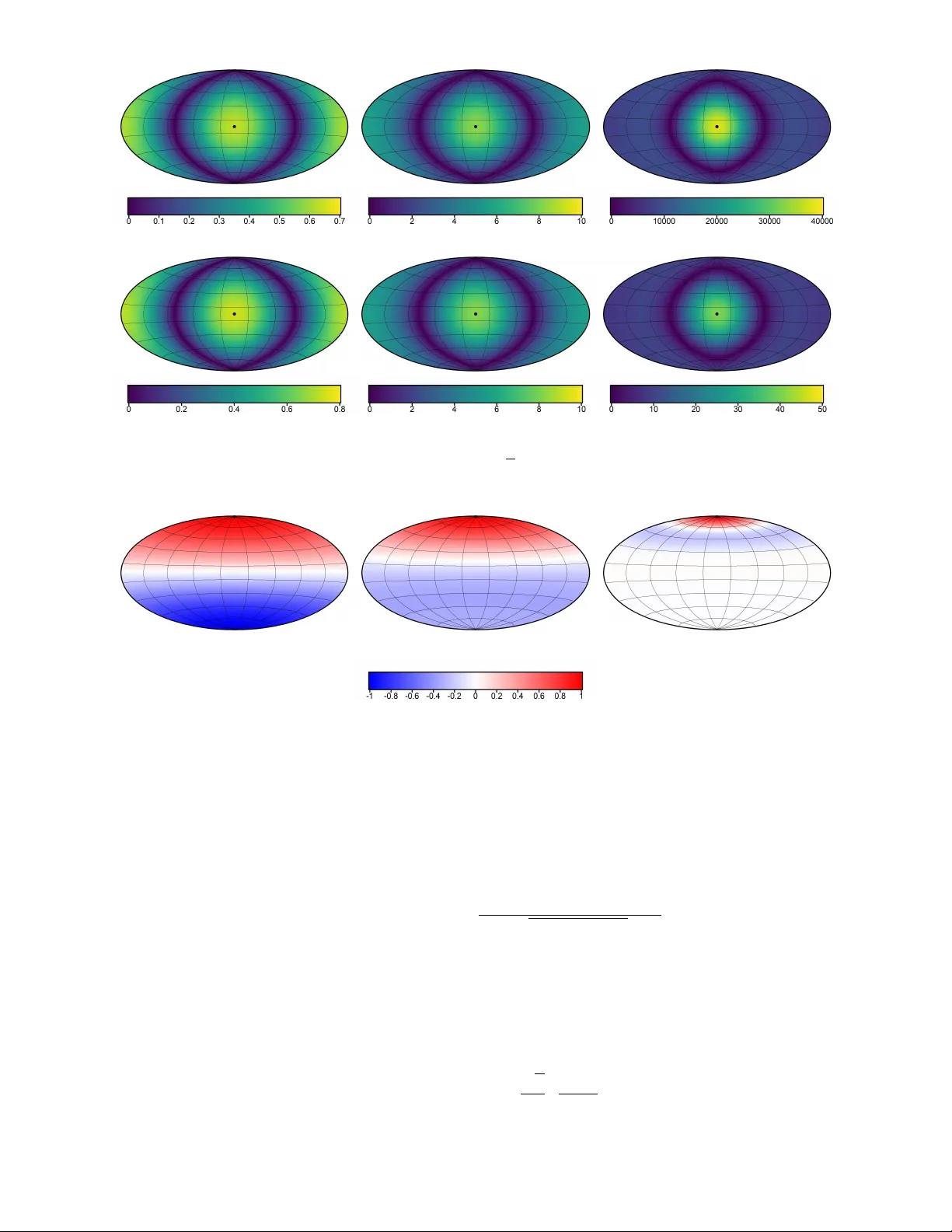
On Stein’s test of uniformit y on the h yp ersphere P aul Axmann 1 , 3 , Bruno Ebner 1 , and Eduardo García-P ortugués 2 Abstract W e prop ose a new test of uniformit y on the hypersphere based on a Stein characterization asso ciated with the Laplace–Beltrami op erator. W e identify a suﬃcien t class of test functions for this characterization, linked to the moment generating function. Exploiting the op erator’s eigenfunctions to obtain a harmonic decomp osition in terms of Gegen bauer p olynomials, w e sho w that the proposed procedure b elongs to the class of Sobolev tests. W e derive closed-form expressions for the distribution of the test statistic under the null hypothesis and under ﬁxed alternativ es. T o enhance p o wer against a range of alternativ es, we introduce a tuning parameter in to the characterization and study its impact on rejection probabilities. W e discuss data-driven strategies for selecting this parameter to maximize rejection rates for a given alternativ e and compare the resulting p erformance with that of related parametric tests. Additional numerical exp erimen ts compare the prop osed test with competing Sob olev-class pro cedures, highlighting settings in whic h it oﬀers clear adv an tages. Keyw ords: Directional data; Laplace–Beltrami op erator; Sob olev tests; Uniformit y; Stein characterization. 1 In tro duction Stein operators oﬀer a p o werful to ol for characterizing probability distributions and can be natu- rally applied to construct go odness-of-ﬁt tests. The use of distributional characterizations to design go odness-of-ﬁt pro cedures dates back to Y u. V. Linnik in the early 1950s (Linnik, 1953a,b; Nikitin, 2017). How ev er, Stein-characterization-based approac hes to testing uniformit y on hyperspheres ha ve only recen tly b egun to be explored, and their relationship to classical uniformit y tests remains under- dev elop ed. Recent works presenting new uni- and m ultiv ariate (Euclidean) pro cedures exploit Stein c haracterizations and build L 2 -t yp e test statistics that quan tify the magnitude of the exp ectation of a Stein op erator ev aluated ov er a characterizing class of functions; see Anastasiou et al. (2023). W e adopt this framework for testing uniformity in directional statistics, where the relev ant Stein op erator is the Laplace–Beltrami op erator, i.e., the spherical comp onen t of the Euclidean Laplacian. Directional statistics concerns observ ations that represent directions; equiv alen tly , it studies random p oin ts supp orted on the unit (h yp er)sphere S p − 1 := { x ∈ R p : ∥ x ∥ = 1 } , where the am bient dimen- sion is p ≥ 2 . F undamental techniques and results are presented in the monographs b y Mardia and Jupp (1999) and Ley and V erdeb out (2017), and recent developmen ts are review ed in P ewsey and García-P ortugués (2021) and García-P ortugués and V erdeb out (2018). When considering directional data, uniformit y is among the most fundamental prop erties to address. F ormally , for an independent and identically distributed (iid) sample X 1 , . . . , X n ∼ P on the sphere, n ∈ N , the hypothesis H 0 : P = Unif ( S p − 1 ) vs. H 1 : P  = Unif ( S p − 1 ) is tested. This classical problem has b een widely studied, with some of the most relev an t tests b eing the Rayleigh (1919) test based on the ﬁrst moments, the Bingham (1974) test based on second order momen ts, and the Giné (1975) F n test, based on an expansion in spherical harmonics. In 1 Institute of Sto c hastics, Karlsruhe Institute of T ec hnology (Germany). 2 Departmen t of Statistics, Carlos I II Universit y of Madrid (Spain). 3 Corresp onding author. e-mail: paul.axmann@kit.edu. 1 addition, more recent prop osals include pro jection-based classes of tests (García-P ortugués et al., 2023; Boro da vk a and Ebner, 2026) and tests based on the Poisson k ernel (F ernández-de-Marcos and García-P ortugués, 2023; Ding et al., 2025). Closely related to our setting, F ernández-de-Marcos and García-P ortugués (2023) also in tro duce a softmax test based on the v on Mises–Fisher k ernel, which in volv es a tuning parameter. Many of these tests b elong to the class of Sob olev tests introduced in Beran (1968) and Giné (1975). Within this common framew ork, Cutting et al. (2017) and Ebner et al. (2025) derive the asymptotic n ull distribution as the dimension div erges to inﬁnity , while García-P ortugués et al. (2026) establishes detection thresholds for rotationally symmetric alterna- tiv es. Another relev an t approac h is the directional k ernel Stein discrepancy (dKSD) test of Xu and Matsuda (2020), emplo ying Stein op erators on the sphere or more general extensions to Riemannian manifolds (Barp et al., 2022; Qu and V emuri, 2025; Xu and Matsuda, 2021). Our c haracterization approach relies on Stein’s metho d (Stein, 1972; Chen et al., 2011), and the prop osed testing pro cedure follows the construction outlined in Anastasiou et al. (2023, Section 5.2). The main idea is to apply a suitable Stein op erator A to a c haracterizing parametric function class F , so that E [ A f ( X )] = 0 holds for all f ∈ F , if and only if the distribution of X satisﬁes the h yp othesis H 0 . This characterization naturally leads to a test statistic b y replacing the exp ectation with its empirical coun terpart. As the empirical mean consistently estimates the expectation, the statistic conv erges to zero under H 0 , while “large” deviations from zero imply rejection of H 0 in fav or of H 1 . In our setting, with a uniform target distribution, a chara cterization induced by the Laplace– Beltrami operator is practically useful: for all smooth functions f , w e hav e E [∆ S p − 1 f ( X )] = 0 exactly for uniformly distributed random unit v ectors X . This is a sp ecial case of the second-order Stein op erator A in Fisc her et al. (2026) and Barp et al. (2022) for general target distributions on S p − 1 with densit y q , whic h can also b e found for lo cal co ordinates in Xu and Matsuda (2021). There, the spherical Stein op erator A f := ∆ S p − 1 f + ⟨∇ log( q ) , ∇ S p − 1 f ⟩ R p , (1) is deriv ed through Green’s ﬁrst iden tity . In the uniform case, the densit y q is constant, implying ⟨∇ log( q ) , ∇ S p − 1 f ⟩ R p = 0 for all f , so the Stein op erator simpliﬁes to the Laplace–Beltrami op erator ∆ S p − 1 . Note that, up to a m ultiplicativ e constant, this Stein op erator coincides with the inﬁnitesimal generator of spherical Bro wnian motion (Hsu, 2002, Chapter 3), whose stationary distribution is the uniform la w on the sphere; it is therefore directly connected to the so-called generator approach to ﬁnd Stein op erators (Barb our, 1988, 1990). T o construct the test statistic, we further need a parametric class of test functions that is ric h enough to characterize the distribution through the Stein iden tity induced b y the op erator. Here, w e c ho ose the class { e λ t ⊤ x : t ∈ S p − 1 } , λ > 0 ﬁxed, connecting the test to the moment generating function (mgf ) M X ( t ) = E  e t ⊤ X  , t ∈ R p . Plugging in this class of test functions leads to the follo wing characterization of the uniform law that we prov e in App endix A. Prop osition 1.1. L et p ≥ 2 and λ > 0 . L et X b e an absolutely c ontinuous r andom ve ctor on S p − 1 . Then, we have the char acterization  E  ∆ S p − 1 e λ t ⊤ X  = ∆ S p − 1 M X ( λ t ) = 0 , t ∈ S p − 1 M X ( 0 ) = 1 , if and only if X ∼ Unif ( S p − 1 ) . (2) T o build a test statistic using this c haracterization of the uniform distribution, we ev aluate the exp ectation E  ∆ S p − 1 e λ t ⊤ X  for all t ∈ S p − 1 . T o this end, we consider the square-integrable map t 7→ E  ∆ S p − 1 e λ t ⊤ X  . More precisely , let ν p − 1 denote the uniform probabilit y measure on S p − 1 , so ν p − 1 ( S p − 1 ) = 1 , and consider the Hilb ert space L 2 ( S p − 1 ) of square-in tegrable functions on the sphere with scalar pro duct ⟨ h, k ⟩ L 2 ( S p − 1 ) = R S p − 1 h ( x ) k ( x ) d ν p − 1 ( x ) for all h, k ∈ L 2 ( S p − 1 ) with the corresp onding norms. Then, we deﬁne the p opulation discrepancy T ( λ ) :=    E  ∆ S p − 1 e λ t ⊤ X     2 L 2 ( S p − 1 ) 2 to characterize the distribution of X . Since rotational inv ariance with resp ect to all rotations about the origin is a well-kno wn characterizing prop ert y of the uniform distribution on the sphere, w e construct a rotation-in v arian t test by uniformly integrating ov er directions using the unw eigh ted L 2 norm. Now, given n ∈ N iid copies X 1 , . . . , X n of the random element X on S p − 1 , we approximate the exp ectation E  ∆ S p − 1 e λ t ⊤ X  b y the empirical mean to prop ose the test statistic T n ( λ ) := n     1 n n X j =1 ∆ S p − 1 e λ t ⊤ X j     2 L 2 ( S p − 1 ) = 1 n n X i,j =1 Z S p − 1 ∆ S p − 1 e λ t ⊤ X i ∆ S p − 1 e λ t ⊤ X j d ν p − 1 ( t ) . (3) This statistic can b e computed eﬃcien tly , through the forthcoming decomp osition (8). The remainder of the pap er is organized as follows. Starting from our Stein-t yp e construction, w e derive a closed-form representation of the prop osed test statistic. Our main to ol is a Gegen- bauer (spherical harmonic) decomp osition of the test functions. Exploiting orthogonality and their connection to the Laplace–Beltrami op erator, we lift the decomp osition from the test-function level to a decomp osition of the en tire statistic, yielding an explicit series expansion. This representation is computationally conv enient, allo ws us to establish the characterization (2) and to develop an asymptotic theory b oth at the level of the underlying pro cess and for the ev aluated statistic. W e treat the null case H 0 as well as ﬁxed alternatives, and provide simpliﬁed expressions for rotationally symmetric alternatives. W e further analyze the eﬀect of tuning, including b oundary/limit regimes. The harmonic viewp oint places the pro cedure within the class of Sob olev tests. W e derive a direct link betw een our Stein test and arbitrary Sob olev tests. In addition, w e compare our metho d to a k ernel Stein discrepancy (dKSD) test, deriv e an analogous harmonic decomp osition for dKSD, and th us obtain the explicit asymptotic results from this test statistic. In sim ulations, we provide plots to illustrate ho w the tuning parameter shapes the co v ariance k ernel and the limiting random ﬁeld predicted by the asymptotic theory . Based on the results from the asymptotic section, w e describ e a tuning approach for the concentration parameter to optimize p ow er against a given alternativ e b y maximizing the standardized mean shift. A cross a range of alternative distributions, we demon- strate its substantial impact on p o wer and empirically v alidate the prop osed tuning strategy . Here, w e further observe the empirical p o wer of the test compared to other uniformit y tests. W e close the pap er with a discussion. Pro ofs are relegated to the app endix. 2 Spherical harmonic decomp osition of the test statistic T o obtain an explicit decomp osition of the test statistic, w e reduce integrals of zonal functions to one-dimensional in tegrals. F or p ≥ 2 , deﬁne L 2 ,p := L 2  [ − 1 , 1] , (1 − u 2 ) ( p − 3) / 2 d u  , ⟨ f , g ⟩ L 2 ,p := Z 1 − 1 f ( u ) g ( u )(1 − u 2 ) ( p − 3) / 2 d u, for f , g ∈ L 2 ,p . In dimension p ≥ 3 , the Gegenbauer p olynomials { C ( p − 2) / 2 k } ∞ k =0 form an orthogonal basis of L 2 ,p , where k denotes the degree of the p olynomial, while in the case p = 2 , the Chebyshev p olynomials C 0 k ( u ) := cos  k arccos( u )  for all k ∈ N 0 form an orthogonal basis of L 2 , 2 . T o unify notation, we denote the Chebyshev p olynomials by { C 0 k } ∞ k =0 , as they form a limit to the Gegenbauer p olynomials, making them a natural c hoice to extend the Gegenbauer construction to the circular case: lim ν → 0 + 1 ν C ν k ( u ) = 2 k C 0 k ( u ) , for k ≥ 1 . 3 F urther, let ω m = 2 π ( m +1) / 2 / Γ  ( m + 1) / 2  denote the Leb esgue surface measure of the unit sphere S m for all m ∈ N . Then, for t , x ∈ S p − 1 and any zonal function f t ( x ) = f ( x ⊤ t ) , the change of v ariables Z S p − 1 f ( x ⊤ t ) d ν p − 1 ( x ) = ω p − 2 ω p − 1 Z 1 − 1 f ( u )(1 − u 2 ) ( p − 3) / 2 d u connects the spaces L 2 ( S p − 1 ) and L 2 ,p , b y reducing in tegrals of zonal functions on S p − 1 to in tegrals on [ − 1 , 1] with the corresp onding w eight. F or t , x ∈ S p − 1 , we consider an orthogonal expansion of the function f λ ( u ) := e λu in L 2 ,p with t ⊤ x = u ∈ [ − 1 , 1] and λ > 0 using Gegen bauer or Cheb yshev p olynomials, dep ending on the dimension. With the co eﬃcien ts deﬁned as m k,p ( λ ) := ⟨ f λ , C ( p − 2) / 2 k ⟩ L 2 ,p   C ( p − 2) / 2 k   2 L 2 ,p , e λu = ∞ X k =0 m k,p ( λ ) C ( p − 2) / 2 k ( u ) , u ∈ [ − 1 , 1] , (4) the orthogonal expansion con verges in L 2 ,p and, for ﬁxed t with u = t ⊤ x , as a function in x in L 2 ( S p − 1 ) , see Dai and Xu (2013, Theorem 2.2.2). F or smo oth functions suc h as the exp onen tial, the co eﬃcien ts deca y rapidly , and the series further conv erges uniformly on [ − 1 , 1] , whic h allo ws term-wise application of the Laplace–Beltrami op erator in the following deriv ations. Remark 2.1. The uniform c onver genc e of e λ t ⊤ x = P ∞ k =0 m k,p ( λ ) C ( p − 2) / 2 k ( t ⊤ x ) holds sinc e x 7→ e λ t ⊤ x is inﬁnitely diﬀer entiable on S p − 1 (Kalf, 1995, The or em 2). T o obtain a closed-form expression of m k,p ( λ ) for p ≥ 3 , we use an integral identit y of Bessel functions 1 h k,p Z 1 − 1 e au C ( p − 2) / 2 k ( u )(1 − u 2 ) ( p − 3) / 2 d u =  2 a  ( p − 2) / 2 Γ  p − 2 2  k + p − 2 2  I ( p − 2) / 2+ k ( a ) , whic h follo ws from Zwillinger et al. (2014, F ormula 7.321) using h k,p = ∥ C ( p − 2) / 2 k ∥ 2 L 2 ,p and a ∈ C \ { 0 } . Here, I k denotes the modiﬁed Bessel function of the ﬁrst kind and order k . The case p = 2 is obtained analogously , b y applying DLMF (2020, 18.3.1) and DL MF (2020, 10.9.2). As a result, setting a = λ > 0 , it follows that m k,p ( λ ) =    (2 − 1 { k =0 } ) I k ( λ ) , p = 2 ,  2 λ  ( p − 2) / 2 Γ  p − 2 2   k + p − 2 2  I ( p − 2) / 2+ k ( λ ) , p > 2 , (5) a quan tity that will app ear throughout the pap er. W e introduce the constant γ k,p :=      1 + 1 { k =0 } 2 , p = 2 , p − 2 2 k + p − 2 , p > 2 , (6) to unify the notation. Using this notation, we use the F unk–Heck e formula (Dai and Xu, 2013, Theorem 1.2.9) to hav e Z S p − 1 C ( p − 2) / 2 k ( t ⊤ x ) C ( p − 2) / 2 k ( y ⊤ t ) d ν p − 1 ( t ) = γ k,p C ( p − 2) / 2 k ( x ⊤ y ) . (7) The series expansion (4) is particularly conv enien t because, for any ﬁxed t ∈ S p − 1 , the Gegen- bauer p olynomials satisfy ∆ S p − 1 C ( p − 2) / 2 k ( t ⊤ x ) = ( − k )( k + p − 2) C ( p − 2) / 2 k ( t ⊤ x ) ; see Prop ert y 2 in Dai 4 and Xu (2013, Section B.2). Hence, the Gegenbauer p olynomials C ( p − 2) / 2 k ( t ⊤ x ) are eigenfunctions of the Laplace–Beltrami op erator ∆ S p − 1 with eigen v alues ( − k )( k + p − 2) . The case p = 2 simpliﬁes further, since the space S 1 is one-dimensional. With x = (cos θ , sin θ ) ⊤ , for a function f on S 1 , the Laplace–Beltrami op erator reduces to ∆ S 1 f ( θ ) = d 2 d θ 2 f ( θ ) see Dai and Xu (2013, Section 1.6.1) and th us the Chebyshev p olynomials satisfy ∆ S 1 C 0 k ( t ⊤ x ) = − k 2 C 0 k ( t ⊤ x ) , hence they are eigenfunctions of the Laplace–Beltrami operator on S 1 corresp onding to the eigenv alues − k 2 . Using the Expansion (4), its uniform conv ergence in [ − 1 , 1] and the linearity of ∆ S p − 1 , w e apply the op erator ∆ S p − 1 to the expansion of e λ t ⊤ x , hence for p ≥ 2 ∆ S p − 1 e λ t ⊤ x = ∆ S p − 1 ∞ X k =0 m k,p ( λ ) C ( p − 2) / 2 k ( t ⊤ x ) = ∞ X k =0 m k,p ( λ )∆ S p − 1 C ( p − 2) / 2 k ( t ⊤ x ) = ∞ X k =0  m k,p ( λ )( − k )( k + p − 2)  C ( p − 2) / 2 k ( t ⊤ x ) holds. With these observ ations, the test statistic tak es the follo wing series represen tation. Its pro of, as with all the pro ofs of the pap er, can b e found in App endix A. Lemma 2.1. L et λ > 0 . Then T n ( λ ) has a harmonic de c omp osition of the form T n ( λ ) = 1 n n X i,j =1 ∞ X k =1 c k,p ( λ ) C ( p − 2) / 2 k ( X ⊤ i X j ) , (8) wher e the c o eﬃcients satisfy c k,p ( λ ) :=  m k,p ( λ ) k ( k + p − 2)  2 γ k,p for k ∈ N , p ≥ 2 . The c o eﬃcients ar e c k,p ( λ ) =    2 k 4 I k ( λ ) 2 , p = 2 , 2 p − 3 λ 2 − p ( p − 2)  k + p − 2 2   Γ  p − 2 2  k ( k + p − 2) I ( p − 2) / 2+ k ( λ )  2 , p > 2 . (9) Lemma 2.1 delivers a closed-form formula of the test statistic in (3). In practice, it is suﬃcien t to consider the truncated series (8), since the co eﬃcien ts c k,p ( λ ) decay exp onentially in k . Obviously , (3) is a Sob olev test in the sense of Giné (1975), for more details, see Section 4.2. In the further analysis, including ﬁxed alternativ e distributions, we in tro duce notation for a general spherical harmonic basis. Let k denote the degree of the spherical harmonics, then the set { Y r,k : r = 1 , . . . , d k,p } spans the degree- k space of spherical harmonics, with dimension d k,p =  p + k − 3 p − 2  +  p + k − 2 p − 2  . Then { Y r,k : k ∈ N 0 , r = 1 , . . . , d k,p } forms an orthonormal basis of the space of spherical harmonics H p with resp ect to the uniform measure ν p − 1 . Since the space of spherical harmonics is dense in L 2 ( S p − 1 ) , the spherical harmonics also form a basis of L 2 ( S p − 1 ) (Dai and Xu, 2013, Theorem 2.2.2.). Details on this construction can b e found in García-Portugués et al. (2026, Section 3). If q ∈ L 2 ( S p − 1 ) is a density on S p − 1 , then it admits the harmonic expansion q ( x ) = ∞ X k =0 d k,p X r =1 β r,k Y r,k ( x ) in L 2 ( S p − 1 ) , (10) 5 with co eﬃcien ts β r,k = Z S p − 1 q ( x ) Y r,k ( x ) d ν p − 1 ( x ) . (11) Note that here the equality is given in the sense that lim n →∞     q − n X k =0 d k,p X r =1 β r,k Y r,k     L 2 ( S p − 1 ) = 0 . 3 Asymptotic results T o analyze the asymptotic b eha vior of the test statistic, w e deﬁne the L 2 ( S p − 1 ) -v alued random elemen t W n : S p − 1 → R b y W n ( t ) := 1 √ n n X i =1 ∞ X k =1  m k,p ( λ )( − k )( k + p − 2)  C ( p − 2) / 2 k ( t ⊤ X i ) , t ∈ S p − 1 , so that T n ( λ ) = ∥ W n ∥ 2 L 2 ( S p − 1 ) . Ob viously { W n ( t ) : t ∈ S p − 1 } is a real-v alued random ﬁeld indexed b y S p − 1 . 3.1 Limits under H 0 W e ﬁrst derive closed-form expressions of the limiting n ull distribution. Since T n ( λ ) can be repre- sen ted as the norm of a sum of iid L 2 -v alued random elements, an application of the cen tral limit theorem in separable Hilb ert spaces (Henze, 2024, Theorem 17.29) and the contin uous mapping theorem are used to prov e the following result. Theorem 3.1. L et p ≥ 2 and let X 1 , . . . , X n b e iid uniformly distribute d r andom ve ctors on the spher e S p − 1 . Then, as n → ∞ , ther e exists a c enter e d Gaussian r andom element W in the Hilb ert sp ac e L 2 ( S p − 1 ) such that W n d − → W , implying T n ( λ ) d − → ∥W ∥ 2 . The c ovarianc e kernel of W is K ( s , t ) = ∞ X k =1 c k,p ( λ ) C ( p − 2) / 2 k ( s ⊤ t ) , s , t ∈ S p − 1 . (12) F rom this result, we derive the limit distribution of the test statistic. Theorem 3.2. F or p ≥ 2 and under H 0 we get the asymptotic distribution T n ( λ ) d − → T ∞ ( λ ) := ∞ X k =1 c k,p ( λ ) γ k,p Z d k,p for n → ∞ , wher e Z d k,p ∼ χ 2 d k,p ar e indep endent and γ k,p is deﬁne d in (6) . F rom Theorem 3.2 and the moments of indep enden t c hi-squared distributions, we deriv e the exp ectation and v ariance of the limiting random v ariable as the series expansions E H 0 [ T ∞ ] = P ∞ k =1 c k,p ( λ ) γ k,p d k,p and V ar H 0 [ T ∞ ] = P ∞ k =1 2  c k,p ( λ ) γ k,p  2 d k,p . T o compute the v ariance of T n ( λ ) under H 0 for a ﬁxed n ∈ N , we use the v ariance form ula for U -statistics, and the fact that w e hav e a centered degenerate kernel and a constant diagonal, to see that the v ariance tak es the form, V ar H 0 [ T n ( λ )] = ( n − 1) 2 2 n ( n − 1) E H 0  ∞ X k =1 c k,p ( λ ) C ( p − 2) / 2 k ( X ⊤ Y )  2  (13) = ∞ X k =1 2 n − 1 n  c k,p ( λ ) γ k,p  2 d k,p . (14) 6 3.2 Fixed alternativ es F or an y random vector X on S p − 1 with ﬁxed densit y q with respect to the uniform measure ν p − 1 , w e deriv e the almost sure limit of T n ( λ ) /n as w ell as the limit distribution of the cen tered test statistic. Giv en a general decomposition of the densit y , as expressed in (10) and (11), we ﬁrst pro vide expansions of M X and z . Lemma 3.1. F or an absolutely c ontinuous r andom ve ctor X on S p − 1 with density q ∈ L 2 ( S p − 1 ) , let t ∈ R p \ { 0 } and s ∈ S p − 1 . Then, in L 2 ( S p − 1 ) , M X ( λ t ) = ∞ X k =0 d k,p X r =1 β r,k m k,p ( λ ∥ t ∥ ) γ k,p Y r,k  t ∥ t ∥  , z ( s ) := ∆ S p − 1 M X ( λ s ) = ∞ X k =1 d k,p X r =1 β r,k m k,p ( λ ) γ k,p ( − k )( k + p − 2) Y r,k ( s ) . No w, b y establishing the almost sure con vergence W n / √ n → z in L 2 ( S p − 1 ) and applying the represen tation from Lemma 3.1 in the pro of in App endix A, w e obtain the almost sure limit of T n ( λ ) /n for n → ∞ . Theorem 3.3. L et p ≥ 2 and let X 1 , . . . , X n b e iid c opies of an absolutely c ontinuous r andom ve ctor X on S p − 1 with density q ∈ L 2 ( S p − 1 ) . Then, T n ( λ ) n a.s. − − → τ = ∥ z ∥ 2 L 2 ( S p − 1 ) = ∞ X k =1 d k,p X r =1 β 2 r,k c k,p ( λ ) γ k,p , as n → ∞ . Remark 3.1. The or em 3.3 implies c onsistency against al l absolutely c ontinuous non-uniform dis- tributions. First, by the char acterization in (2) , z ≡ 0 if and only if X is uniformly distribute d on S p − 1 and thus τ > 0 for al l alternative distributions. This c onsistency is also observe d in the Ge genb auer de c omp osition of The or em 3.3, sinc e c k,p ( λ ) γ k,p > 0 implies that, for al l densities q , z ≡ 0 if and only if β r,k = 0 for al l k ≥ 1 , which again implies uniformity. These observations c onne ct to Sob olev test the ory (Giné, 1975, The or em 4.4) sinc e the c o eﬃcients c k,p ( λ ) ar e p ositive for al l k ∈ N . With the same arguments as in Theorem 3.3, we deriv e the exp ectation for ﬁxed n as a series of spherical harmonics. Remark 3.2. As a r esult fr om the pr o of of The or em 3.3, we obtain E [ T n ( λ )] = ( n − 1) ∞ X k =1 d k,p X r =1 β 2 r,k c k,p ( λ ) γ k,p + ∞ X k =1 c k,p ( λ ) C ( p − 2) / 2 k (1) . F o cusing further on the underlying random ﬁeld, w e ﬁnd the limit Gaussian ﬁeld (after recen tering b y the exp ectation) in analogy to Theorem 3.1. W e in tro duce the notation ∆ S p − 1 , t to denote the Laplace–Beltrami op erator on S p − 1 acting with resp ect to the v ariable t ∈ S p − 1 . Theorem 3.4. L et p ≥ 2 and let X 1 , . . . , X n b e iid c opies of an absolutely c ontinuous r andom ve ctor X on S p − 1 with density q . Then ther e exists a r e al-value d c enter e d Gaussian r andom element W ′ in L 2 ( S p − 1 ) for which  W n − √ nz  d − → W ′ holds for n → ∞ , and wher e W ′ has the c ovarianc e kernel K ′ ( s , t ) = ∆ S p − 1 , s ∆ S p − 1 , t M X  λ ( s + t )  − ∆ S p − 1 M X ( λ s )∆ S p − 1 M X ( λ t ) 7 = ∞ X k 1 =0 ∞ X k 2 =0  m k 1 ,p ( λ )( − k 1 )( k 1 + p − 2)  m k 2 ,p ( λ )( − k 2 )( k 2 + p − 2)  ξ k 1 ,k 2 ( s , t ) − z ( s ) z ( t ) . Her e, we write ξ k 1 ,k 2 ( s , t ) = E  C ( p − 2) / 2 k 1 ( s ⊤ X ) C ( p − 2) / 2 k 2 ( t ⊤ X )  for al l s , t ∈ S p − 1 . F or applications, it is con venien t to consider a ﬁnite-dimensional pro jection of the random ﬁeld W ′ to get a cov ariance matrix corresp onding to the k ernel at a ﬁxed set of vectors on the sphere. Remark 3.3. L et m ∈ N and ﬁx t 1 , . . . , t m ∈ S p − 1 . F or k ∈ N , deﬁne the ve ctors of Ge genb auer p olynomials and spheric al harmonics as C k ( x ) :=  C ( p − 2) / 2 k ( t ⊤ 1 x ) , . . . , C ( p − 2) / 2 k ( t ⊤ m x )  ⊤ and Y r,k :=  Y r,k ( t 1 ) , . . . , Y r,k ( t m )  ⊤ . This notation al lows us to write the c ovarianc e matrix K m of the Gaussian limit of the r andom ve ctor W n − √ n z :=  W n ( t 1 ) − √ nz ( t 1 ) , . . . , W n ( t m ) − √ nz ( t m )  ⊤ , c orr esp onding to the kernel K ′ in The or em 3.4, as v ec ( K m ) = E  ∞ X k =1  m k,p ( λ )( − k )( k + p − 2)   C k ( X ) − γ k,p d k,p X r =1 β r,k Y r,k  ⊗ 2  = E  ∞ X k =1  m k,p ( λ )( − k )( k + p − 2)  C k ( X )  ⊗ 2  − z ⊗ 2 , wher e z ⊗ 2 = z ⊗ z = v ec  z z ⊤  . The entries of K m ar e ( K m ) i,j = K ′ ( t i , t j ) . Although this representation is more practical, it cannot b e expressed in closed form, as the exp ectation ξ k 1 ,k 2 has to b e ev aluated at diﬀerent v ectors s , t with s  = t . Restricting to the case s = t , the exp ectation can b e expressed using the linearization form ula for Gegenbauer p olynomials (24), leading to a closed expression for the v ariance function of the random ﬁeld. Remark 3.4. L o oking at the varianc e function of W ′ in a dir e ction s ∈ S p − 1 with the line arization formula (24) yields the close d expr ession ξ k 1 ,k 2 ( s , s ) = min( k 1 ,k 2 ) X ℓ =0 L ( p ) k 1 ,k 2 ( ℓ ) γ k 1 ,p + k 2 − 2 ℓ d k 1 ,p + k 2 − 2 ℓ X r 3 =1 β r 3 ,k 1 + k 2 − 2 ℓ Y r 3 ,k 1 + k 2 − 2 ℓ ( s ) . Using the limit distribution of the random ﬁeld W n in Theorem 3.4, we derive the limit distri- bution of the centered test statistic. Theorem 3.5. L et p ≥ 2 and let X 1 , . . . , X n b e iid c opies of a r andom ve ctor X on S p − 1 S p − 1 with density q . Then √ n  T n ( λ ) n − τ  d − → N (0 , σ 2 ) , with σ 2 = 4 Z S p − 1 Z S p − 1 K ′ ( s , t ) z ( s ) z ( t ) d ν p − 1 ( s ) d ν p − 1 ( t ) = 4 E  ∞ X k =1 d k,p X r =1 γ k,p c k,p ( λ ) β r,k  Y r,k ( X ) − β r,k   2  . 8 3.3 Rotationally symmetric alternatives W e specialize the general alternative theory to the imp ortan t class of rotationally symmetric alter- nativ es ab out a ﬁxed direction µ ∈ S p − 1 . The key adv antage of rotational symmetry is that it allows for simpliﬁcations of the spherical harmonic decomp osition. It is suﬃcient to decomp ose the densit y in Gegen bauer p olynomials, due to the zonal structure. F or a zonal densit y q , there is an angular function g : [ − 1 , 1] → R so that we ﬁnd the Gegenbauer decomp osition, q ( x ) = g ( µ ⊤ x ) = ∞ X k =0 β k C ( p − 2) / 2 k ( µ ⊤ x ) , β k = Z S p − 1 q ( x ) C ( p − 2) / 2 k ( µ ⊤ x ) d ν p − 1 ( x ) . As an example, we explicitly deriv e the co eﬃcien ts β k in closed form for for the von Mises–Fisher (vMF) distribution. Example 3.1. L et κ > 0 and µ ∈ S p − 1 , and denote by f vMF ( · ; µ , κ ) the density of the von Mises– Fisher distribution vMF( µ , κ ) with r esp e ct to ν p − 1 , so f vMF ( x ; µ , κ ) = κ ( p − 2) / 2 ω p − 1 (2 π ) p/ 2 I ( p − 2) / 2 ( κ ) e κ µ ⊤ x , for al l x ∈ S p − 1 . Combining (5) and (4) , we obtain the de c omp osition f vMF ( x ; µ , κ ) = κ ( p − 2) / 2 ω p − 1 (2 π ) p/ 2 I ( p − 2) / 2 ( κ ) ∞ X k =0 m k,p ( κ ) C ( p − 2) / 2 k ( µ ⊤ x ) . This implies the Ge genb auer c o eﬃcients admit the explicit form β k = κ ( p − 2) / 2 ω p − 1 (2 π ) p/ 2 I ( p − 2) / 2 ( κ ) m k,p ( κ ) , k ∈ N 0 . (15) The results in Lemma 3.1 and Theorem 3.3 simplify by exploiting the Gegen bauer decomp osition. Remark 3.5. Under the assumption of r otational symmetry, we ﬁnd with the same ar guments use d in the pr o of of L emma 3.1 that z ( s ) = ∞ X k =1 β k m k,p ( λ ) γ k,p ( − k )( k + p − 2) C ( p − 2) / 2 k ( µ ⊤ s ) , s ∈ S p − 1 . (16) The limit τ as deﬁne d in The or em 3.3, simpliﬁes to T n ( λ ) n a.s. − − → τ = ∞ X k =1 ( β k γ k,p ) 2 c k,p ( λ ) C ( p − 2) / 2 k (1) . Her e, the factor γ k,p C ( p − 2) / 2 k (1) arises fr om taking the inte gr al with r esp e ct to ν p − 1 of C ( p − 2) / 2 k ( µ ⊤ t ) 2 , via the F unk–He cke formula and exploiting the ortho gonal r elation of the Ge genb auer p olynomials (7) . F urther, the results for the random ﬁeld W n are simpliﬁed. A key adv antage in these remarks is that the spherical harmonic co eﬃcien ts β k are determined in explicit form for alternativ es such as the vMF distribution, so the asymptotic distribution is av ailable without n umerically approximating the co eﬃcien ts β r,k . Remark 3.6. With the same notation as in R emark 3.3 we write the c ovarianc e matrix K m , c or- r esp onding to the kernel K ′ in The or em 3.4, as v ec ( K m ) = E  ∞ X k =1  m k,p ( λ )( − k )( k + p − 2)  C k ( X ) − γ k,p β k C k ( µ )   ⊗ 2  . (17) 9 Mor e gener al ly, for two ﬁxe d ve ctors s , t ∈ S p − 1 , the kernel is expr esse d as K ′ ( s , t ) = ∞ X k 1 =0 ∞ X k 2 =0  m k 1 ,p ( λ )( − k 1 )( k 1 + p − 2)  m k 2 ,p ( λ )( − k 2 )( k 2 + p − 2)  ×  ξ k 1 ,k 2 ( s , t ) − γ k 1 ,p γ k 2 ,p β k 1 β k 2 C ( p − 2) / 2 k 1 ( µ ⊤ s ) C ( p − 2) / 2 k 2 ( µ ⊤ t )  . Remark 3.7. In this setting, we simplify the expr ession of the varianc e fr om The or em 3.5, similar to R emark 3.6, and get σ 2 = 4 E  ∞ X k =1 γ k,p c k,p ( λ ) β k  C ( p − 2) / 2 k ( µ ⊤ X ) − β k γ k,p C ( p − 2) / 2 k (1)   2  = 4  ∞ X k 1 =0 ∞ X k 2 =0 γ k 1 ,p c k 1 ,p ( λ ) β k 1 γ k 2 ,p c k 2 ,p ( λ ) β k 2 min( k 1 ,k 2 ) X ℓ =0 β k 1 + k 2 − 2 ℓ L ( p ) k 1 ,k 2 ( ℓ ) γ k 1 + k 2 − 2 ℓ,p C ( p − 2) / 2 k 1 + k 2 − 2 ℓ (1) −  ∞ X k =1 d k,p X r =1 ( β r,k ) 2 γ k,p c k,p ( λ ) C ( p − 2) / 2 k (1)  2  . Her e, the last e quality holds by applying the line arization formula (24) on the p olynomials C ( p − 2) / 2 k ( µ ⊤ X ) , yielding a close d-form expr ession. This expr ession is derive d in the pr o of of The or em 3.5 in Ap- p endix A. 4 Connections to other tests 4.1 Limit b eha vior of the test for λ → 0 and λ → ∞ The p o w er of the test based on T n ( λ ) is sensitiv e to diﬀerent choices of λ , se e Figure 5. In the follo wing proposition, w e analyze the limit b eha vior of the test statistic for extreme v alues of λ and ﬁxed sample size n . Here, we use the sto c hastic Landau sym b ols, so X n = o P (1) denotes the con vergence in probability of X n to zero. Prop osition 4.1. Fix n ∈ N and X 1 , . . . , X n iid on S p − 1 . As λ → 0 and λ → ∞ the r eje ction rule b ase d on T n ( λ ) is asymptotic al ly e quivalent to i. the R ayleigh (1919) test for λ → 0 , sinc e lim λ → 0 λ − 2 T n ( λ ) ∝ 1 n P n i,j =1 X ⊤ i X j ; ii. the Cai et al. (2013) test for λ → ∞ , sinc e, for D n ( λ ) := 1 n P n j =1   ∆ S p − 1 e λ t ⊤ X j   2 L 2 ( S p − 1 ) , lim λ →∞ λ − 1 log  T n ( λ ) − D n ( λ )  = max 1 ≤ i 0 , the represen tation in (9) assigns p ositive weigh t to all orders k . This limit behavior for λ coincides with the behavior observ ed in the softmax test ( S n ( κ ) ) in tro duced in F ernández-de-Marcos and García-P ortugués (2023) with tuning parameter κ . F or an y ﬁxed λ = κ ∈ (0 , ∞ ) , the Gegen bauer coeﬃcients of T n ( λ ) and S n ( λ ) diﬀer by a factor of m k,p ( λ )  k ( k + p − 2)  2 γ k,p . Since this factor decays rapidly as k → ∞ for ﬁxed λ , T n ( λ ) places the ma jority of its weigh t on a smaller range of indices k than the softmax test. Moreov er, for any tuning parameters κ, λ in (0 , ∞ ) , S n ( κ ) cannot b e recov ered from T n ( λ ) , by any reparameterization of λ . 10 Remark 4.1. A l lowing for a c omplex tuning p ar ameter λ ∈ C links the c onstruction to the char ac- teristic function of the distribution, in p articular for pur ely imaginary ar guments iλ . The r esulting c o eﬃcients c k,p ( iλ ) ar e obtaine d fr om the c o eﬃcients c k,p ( λ ) , by r eplacing the mo diﬁe d Bessel func- tion of the ﬁrst kind I with the Bessel function of the ﬁrst kind J , r eﬂe cting the oscil lating structur e of the char acteristic function in c ontr ast to the exp onential gr owth of the mgf. 4.2 Connections to Sob olev tests A v ery rich family of tests of uniformit y on S p − 1 is giv en by the Sob olev tests. Multiple equiv alent represen tations and deﬁnitions illustrate the connections to our construction. First, w e can deﬁne the Sob olev tests through the harmonic decomp osition of the zonal kernel, where it is again con venien t that the spherical harmonics form eigenfunctions of our Stein op erator. Remark 4.2. L et X 1 , . . . , X n iid on S p − 1 and deﬁne θ i,j = arccos( X ⊤ i X j ) . The class of Sob olev test statistics by Ber an (1968), Giné (1975), and Pr entic e (1978) has the form S n,p ( { w k,p } ) = 1 n n X i,j =1 ψ ( θ i,j ) , ψ ( θ ) = ∞ X k =1 w k,p γ k,p C ( p − 2) / 2 k (cos θ ) . With represen tation (8), it b ecomes clear that T n ( λ ) is a mem b er of the class of Sob olev test statistics, since for cos θ i,j = X ⊤ i X j w e see that the Sob olev weigh ts are given as w λ k,p = γ k,p c k,p ( λ ) . A diﬀeren t view on the Sob olev test statistic considers a L 2 distance on an angular function g (Beran, 1968; Giné, 1975). Here, the Sob olev test, whic h is the lo cally most p o w erful rotation- in v arian t test for testing H 0 against alternativ es with densit y g ( · ⊤ µ ) , is given by S n,p ( { ψ } ) = 1 n     n X i =1 g ( X ⊤ i · ) − n     2 L 2 ( S p − 1 ) . (18) The connection of ψ to the Gegenbauer expansion in Remark 4.2 is g ( z ) := 1 + ∞ X k =1 √ w k,p γ k,p C ( p − 2) / 2 k ( z ) , z ∈ [ − 1 , 1] . W e now obtain representations of general Sob olev tests as L 2 -Stein tests indexed by function classes { f t : t ∈ S p − 1 } more general than the exp onen tial class. Consider a Sob olev test statis- tic S n,p ( { ψ } ) with kernel ψ ( θ ) = P ∞ k =1 b k,p C ( p − 2) / 2 k (cos θ ) , where p ≥ 2 and b k,p ≥ 0 . F or the corresp onding function class { f t : t ∈ S p − 1 } with f t ( x ) = ∞ X k =1 p b k,p k ( k + p − 2) √ γ k,p C ( p − 2) / 2 k ( t ⊤ x ) , the statistic S n,p ( { ψ } ) admits the representation S n,p ( { ψ } ) = 1 n     n X i =1 ∆ S p − 1 f t ( X i )     2 L 2 ( S p − 1 ) . No w, for the angular function g of (18), we see g ( x ⊤ t ) = 1 − ∆ S p − 1 f t ( x ) , using the eigenfunction relation of Gegenbauer p olynomials for ∆ S p − 1 . 11 4.3 Connections to the dKSD 2 (2) test There are diﬀerent wa ys to deﬁne a test statistic based on a Stein op erator. T o con trast the prop osed L 2 -Stein approach, we consider a directional kernel Stein discrepancy test with the same op erator and k ernel functions and compare the resulting structures. The application of a kernel Stein discrepancy (KSD) in a directional setting has b een considered in Xu and Matsuda (2020). F or the iid random v ectors X 1 , . . . , X n with unknown densit y q and target density d , with Stein op erator A d , the dKSD V -statistic tak es the form dKSD 2 (2) = 1 n 2 n X i,j =1 h d ( X i , X j ) , where h d ( x , y ) = ⟨A d k ( x , · ) , A d k ( y , · ) ⟩ H , (19) see Xu and Matsuda (2020, Equation (13)). While Xu and Matsuda (2020) uses a ﬁrst-order Stein op erator A , here we consider the second-order Stein op erator deﬁned in (1), which w e denote by the subscript (2) in (19). In Xu and Matsuda (2021), a v ersion of KSD using a second-order Stein operator in lo cal co ordinates is discussed in a more general setting on manifolds with empt y b oundary . Considering a KSD construction on the sphere and for the uniform target distribution with constan t density d , w e obtain the k ernel h d ( x , y ) = ∆ S p − 1 , x ∆ S p − 1 , y k ( x , y ) . Here, we use the repro ducing kernel property and apply the simpliﬁed op erator from (1). T o connect this construction to our L 2 -Stein construction, we ﬁx the k ernel to b e the v on Mises–Fisher kernel k ( x , y ) = e λ x ⊤ y with λ > 0 . Consequently , the same Gegen bauer expansion in (5) is used to decomp ose the kernel, and w e derive a closed Gegen bauer representation dKSD 2 (2) = 1 n 2 n X i,j =1 ∞ X k =1 c dKSD k,p ( λ ) C ( p − 2) / 2 k ( X ⊤ i X j ) , with similar Gegen bauer co eﬃcien ts c dKSD k,p ( λ ) := m k,p ( λ )  k ( k + p − 2)  2 . This analogous represen- tation helps iden tify the eﬀect of the t wo constructions. It also directly allows for application of our asymptotic results from Section 3, after replacing the co eﬃcien ts c k,p ( λ ) b y c dKSD k,p ( λ ) . Hence, we pro vide a direct method to compute the asymptotic distribution of the test statistic, b oth under H 0 and under ﬁxed alternatives, incorp orate the p erspective of the underlying random ﬁeld to analyze the test, and show that the test b elongs to the class of Sob olev tests. The coeﬃcients of the L 2 -Stein and dKSD 2 (2) tests diﬀer b y a factor of c k,p ( λ ) /c dKSD k,p ( λ ) = γ k,p m k,p ( λ ) . T o illustrate this diﬀerence, we plot standardized v ersions of the functions k 7→ c k,p ( λ ) and k 7→ c dKSD k,p ( λ ) in Figure 1. The w eight of the L 2 -Stein test is more concen trated on a narro w set of indices compared to the dKSD 2 (2) test, while the concen tration parameter λ has a similar eﬀect in b oth approaches, shifting the w eight of the tests to Gegen bauer p olynomials of higher order as λ increases. 5 Numerical exp eriments 5.1 Visualization of cov ariance under alternatives In this section, we visualize the structure of the limiting Gaussian pro cesses obtained in Theorem 3.1 and in Theorem 3.4. These are, resp ectiv ely , W and W ′ , the limit of the empirical pro cesses W n − √ nz . T o do so, we explore the shap e of: ( i ) the centering s 7→ √ nz ( s ) under a ﬁxed alternative ( z ( s ) ≡ 0 under H 0 ); ( ii ) the null correlation k ernel s 7→ ρ ( s , t ) := K ( s , t ) / p K ( s , s ) K ( t , t ) ; and ( iii ) the ﬁxed-alternative correlation k ernel s 7→ ρ ′ ( s , t ) . These explorations shed ligh t on what 12 parts of the sphere con tribute the most to increasing the exp ectation of the test statistic and detect a ﬁxed alternativ e, and into ho w the correlation structure of the random ﬁeld W changes into that of W ′ . 0 2 4 6 8 10 0.0 0.2 0.4 0.6 0.8 1.0 k Relative coefficients λ = 1 λ = 3 λ = 5 λ = 10 L 2 dKSD (a) p = 3 0 2 4 6 8 10 0.0 0.2 0.4 0.6 0.8 1.0 k Relative coefficients λ = 1 λ = 3 λ = 5 λ = 10 L 2 dKSD (b) p = 10 Figure 1: Relative coeﬃcients k 7→ c k,p ( λ ) and k 7→ c dKSD k,p ( λ ) for dimensions p = 3 and p = 10 , for the L 2 - Stein test (solid lines) and the dKSD test (dashed lines). F or each c hoice of λ , the coeﬃcients are standardized b y their maximum. T o illustrate the eﬀect, we plot the con tinuous mappings in k , while in the test, only ev aluations at integer v alues of k are used. T o visualize the previous functions, we use the equal-area Hammer pro jection to map S 2 to an elliptical pro jection, displaying also selected parallels and meridians. W e consider the vMF( µ , κ ) distribution as a ﬁxed alternative to leverage the expressions (16) and (17) and compute K ′ ( s , t ) and z ( s ) using the explicit form for the vMF co eﬃcien ts in (15). W e set µ = (0 , − 1 , 0) ⊤ . F or computing K ( s , t ) , w e used (12). The series in z ( s ) , K ( s , t ) , and K ′ ( s , t ) w ere truncated to their ﬁrst 100 terms. T o compute (17) we used Mon te Carlo with M = 10 , 000 replicates. Figure 2 sho ws s 7→ √ n | z ( s ) | , illustrating the eﬀects that λ and κ hav e on its structure. The larger λ , the larger the relativ e weigh t of | z ( s ) | at ab out s = µ (Figure 2c), with the relative w eight at the antipo dal region (see Figure 2a) disapp earing. This eﬀect parallels the relative concentration eﬀect of larger κ (Figures 2d–2f). The v alue of | z ( s ) | at s = µ and, implied by that, the v alue of ∥ z ∥ 2 L 2 ( S p − 1 ) , increases monotonically with λ , as manifested in the increasing upp er limits of the legends in Figures 2a–2c. The n ull correlation k ernel s 7→ ρ ( s , t ) is shown in Figure 3 for t = (0 , 0 , 1) ⊤ . The kernel only dep ends on s ⊤ t (i.e., it is isotropic). Increasing λ has the eﬀect of lo calizing the range of the correla- tion kernel at s = t . This happ ens b oth for p ositive and negativ e correlations. P ositive correlations are lo cated at the northern hemisphere, for λ close to zero (Figure 3a), and then concen trate at s = t for large λ (Figure 3c). Negativ e correlations are lo cated on the southern hemisphere for small λ , but then are attracted to parallels close to the north p ole for large λ . Indeed, for large λ , near-zero correlations app ear at the south pole and southern hemisphere. Finally , Figure 4 shows the ﬁxed-alternativ e correlation kernel s 7→ ρ ′ ( s , t ) , now dep endent on ( s ⊤ t , µ ⊤ s , µ ⊤ t ) , for µ = (0 , − 1 , 0) ⊤ and t = (0 , 0 , 1) ⊤ . F or κ = 1 , the non-isotrop y is subtle, with the eﬀects of µ b eing very mild, and the correlations resem ble those in Figure 3. The non-isotrop y b ecomes evident for κ = 10 , where µ aﬀects the correlation ﬁeld with the ﬁeld v alue at s dep ending on the angle b et w een s and µ . Strong p ositiv e correlations are still maintained at s = t , as exp ected. 13 (a) κ = 1 , λ = 0 . 1 (b) κ = 1 , λ = 1 (c) κ = 1 , λ = 10 (d) κ = 0 . 1 , λ = 1 (e) κ = 1 , λ = 1 (f ) κ = 10 , λ = 1 Figure 2: Hammer pro jection represen tation of s 7→ √ n | z ( s ) | , for the ﬁxed alternative vMF( µ , κ ) and n = 100 . The central p oin t is µ = (0 , − 1 , 0) ⊤ . In the ﬁrst ro w, κ = 1 is ﬁxed, while in the second, λ = 1 is. (a) λ = 0 . 1 (b) λ = 1 (c) λ = 10 Figure 3: Hammer pro jection representation of the n ull correlation kernel s 7→ ρ ( s , t ) , for t = (0 , 0 , 1) ⊤ (north pole, diamond). The shap e of the kernel is inv ariant from the c hoice of t . 5.2 P arameter selection The testing pro cedure can b e adapted to a sp eciﬁc alternative by selecting the tuning parameter λ that maximizes the rejection rate under the underlying distribution. T o optimize the parameter λ w e consider the standardized mean shift under H 1 , compared to H 0 : ˆ λ = arg max λ> 0 q λ = arg max λ> 0 E H 1 [ T n ( λ )] − E H 0 [ T n ( λ )] p V ar H 0 [ T n ( λ )] . Maximizing this expression corresp onds to maximizing the rejection rate for a given alternative; see Gregory (1977). Here, we approximate the exp ectation E H 1 [ T n ( λ )] with the observ ed v alue of T n ( λ ) , while (14) provides closed expressions for E H 0 [ T n ( λ )] and V ar H 0 [ T n ( λ )] . Alternativ ely , using Theorem 3.5 and incorporating the critical v alue c n ( λ ) , an estimate of the p o w er function (see Baringhaus et al. (2017, Section 3.2)) can b e obtained as P H 1 ( T n  λ ) > c n ( λ )  ≈ 1 − Φ  √ n σ  c n ( λ ) n − τ   . F or simpliﬁed computation, we use the score function q λ . 14 (a) κ = 1 , λ = 0 . 1 (b) κ = 1 , λ = 1 (c) κ = 1 , λ = 10 (d) κ = 10 , λ = 0 . 1 (e) κ = 10 , λ = 1 (f ) κ = 10 , λ = 10 Figure 4: Hammer pro jection representation of the ﬁxed-alternativ e correlation kernel s 7→ ρ ′ ( s , t ) , for the ﬁxed alternativ e vMF( µ , κ ) and t = (0 , 0 , 1) ⊤ (north pole, diamond). The cen tral p oin t is µ = (0 , − 1 , 0) ⊤ . The concen tration parameter λ only aﬀects the test statistic through the co eﬃcien ts c k,p ( λ ) . T o eﬃcien tly compute the test statistic for a wide range of λ v alues, it is con venien t to rearrange the summation to T n ( λ ) = ∞ X k =1 c k,p ( λ ) A k , A k = 1 n n X i,j =1 C ( p − 2) / 2 k ( X ⊤ i X j ) , with A k indep enden t of λ . No w, to estimate the expectation of the test statistic E [ T n ( λ )] = P ∞ k =1 c k,p ( λ ) E [ A k ] for an y λ , w e estimate E [ A k ] = ( n − 1) E  C ( p − 2) / 2 k ( X ⊤ 1 X 2 )  + C ( p − 2) / 2 k (1) . Giv en an iid sample Y 1 , . . . , Y N , N ∈ N , distributed as X , this allo ws us to compute an appro ximation of E [ A k ] , ¯ A k = ( n − 1) 1 N ( N − 1) X 1 ≤ i  = j ≤ N C ( p − 2) / 2 k ( Y ⊤ i Y j ) + C ( p − 2) / 2 k (1) once in adv ance, to then allo w for direct ev aluation of the test statistic dep ending on λ . Then with ¯ T n ( λ ) = P ∞ k =1 c k,p ( λ ) ¯ A k , w e deﬁne ˜ λ = arg max λ> 0 ¯ T n ( λ ) − E H 0 [ T n ( λ )] p V ar H 0 [ T n ( λ )] . (20) Note that this approach yields an appro ximate choice of the tuning parameter, which relies on an indep enden t sample from the alternative distribution. In the following section, w e implemen t this selection approach b y searc hing λ ov er the grid { i/ 10 : i ∈ { 1 , . . . , 300 }} . T o appro ximate the required co eﬃcien ts, w e use 10 , 000 indep enden t dra ws from the candidate density q . F or many rotationally symmetric alternativ es, the co eﬃcien ts β k admit closed-form expressions, for kno wn distributions, see Example 3.1 for the von Mises–Fisher distribution. The corresp onding exp ectation can then b e deriv ed using Remark 3.2. In practice, ho wev er, indep enden t sampling from the underlying alternative is una v ailable, so these quantities must b e estimated from the observed data. A standard approac h is cross-v alidation, for which w e refer to the pro cedure describ ed in F ernández-de-Marcos and García-Portug ués (2023, Section 4). In T able 1, w e compare the rejection rate of the oracle parameter test with the K - fold test, dep ending only on the observ ations. Here we use alternatives described in the following subsection. 15 vMF(0 . 5) W(1) SC(0 . 5) MvMF(5) T est 50 100 50 100 50 100 50 100 T n ( ˜ λ ) 36 . 52 65 . 10 31 . 78 62 . 42 26 . 58 55 . 22 17 . 22 32 . 14 T n, 20 ( λ ) 23 . 90 53 . 38 17 . 46 38 . 10 17 . 94 44 . 70 9 . 28 17 . 90 T able 1: Empirical rejection rates in p = 3 with M = 5 , 000 Mon te Carlo samples at signiﬁcance level α = 5% of the oracle parameter test T n ( ˜ λ ) and the 20 -fold cross-v alidation test T n, 20 ( λ ) . Sample sizes are 50 and 100 . 5.3 Comparison to other tests In the follo wing, we compare the p o wer of the proposed test statistic against a selection of alternative distributions and b enc hmark it against diﬀeren t Sobolev tests of uniformity . T o that end, we consider the test statistic T n ( ˜ λ ) with the optimized parameter ˜ λ deﬁned in (20), and the test statistic T n ( λ ) for ﬁxed v alues λ ∈ { 1 , 4 } . The tests considered in the comparison are the Giné (1975) F n test ( F n ), the Bingham (1974) test ( B n ), the Rayleigh (1919) test ( R n ), the softmax test ( S n ) from F ernández- de-Marcos and García-P ortugués (2023), and the Pro jected Anderson–Darling test ( P AD ) from García-P ortugués et al. (2023). The comparison is p erformed for dimensions p = 2 , 3 , 5 and sample sizes n = 50 and n = 100 . W e structure the comparison by ﬁrst considering unimodal alternativ es. Here, w e set µ := e 1 with a von Mises–Fisher distribution f vMF ( x ; µ , κ ) ∝ e κ µ ⊤ x with concen tration parameter κ = 0 . 5 and a Cauch y-like distribution f Ca ( x ; µ , κ ) =  1 − ρ ( κ ) 2 1 − 2 µ ⊤ x ρ ( κ ) + ρ ( κ ) 2  p with ρ ( κ ) = 2 κ + 1 − √ 4 κ + 1 2 κ , x ∈ S p − 1 , with concentration parameter κ = 0 . 25 . W e denote these alternatives by vMF(0 . 5) and Ca(0 . 25) , resp ectiv ely . Next axial data is considered. On the one hand, we sample from the W atson distribution f W ( x ; µ , κ ) ∝ e κ ( µ ⊤ x ) 2 with κ = 1 (denoted W(1) ). On the other hand from an unbalanced mixture of t wo von Mises–Fisher distributions vMF(2 , e 1 ) and vMF(2 , − e 1 ) , at opp osite p oles, f vMFM ( x ; q ) = (1 − q ) f vMF ( x ; e 1 , 2) + q f vMF ( x ; − e 1 , 2) , x ∈ S p − 1 , with q = 0 . 3 ( vMFM(0 . 3) ). A small circle distribution f SC ( x ; κ, ν ) ∝ e − κ ( e ⊤ 1 x − ν ) 2 , concentrated around a mo dal lo wer di- mensional subsphere, with κ = 0 . 5 and ν = 0 . 5 is also considered ( SC(0 . 5 , 0 . 5) ). T o deﬁne alternatives obtained by rotating rotat ionally symmetric distributions, let R i,j ( α ) denote the rotational matrix in the ( i, j ) -plane with rotation angle α . With SCM(3) , we denote a distribution of k = 3 uniformly w eighted copies of distributions SC(10 , 0) , rotated b y an angle ( j /k )2 π for j ∈ [ k ] in the (2 , 3) -plane: f SCM ( x ; k ) = k X j =1 1 k f SC  R 2 , 3  − j k 2 π  x ; 10 , 0  , x ∈ S p − 1 . Analogously , pro jNM(5) denotes a mixture of k uniformly weigh ted rotated copies of a pro jected normal distribution. In eac h sample, w e generate from N (4 e 1 , Σ ) with the diagonal cov ariance matrix Σ = I d + 9 e d , the resulting vectors are pro jected onto the unit sphere and rotated. First, w e deﬁne the densit y of the pro jected normal distribution f pro jN ( x ) ∝ Z ∞ 0 r p − 1 exp  − 1 2 ( r x − 4 e 1 ) ⊤ Σ ( r x − 4 e 1 )  d r , x ∈ S p − 1 , 16 to then obtain the density of the mixture of rotated pro jected normal distributions, as f pro jNM ( x ) = k X j =1 1 k f pro jN  R 1 , 2  − j k 2 π  x  , x ∈ S p − 1 . A t last, with MvMF(30) we denote a distribution consisting of an equal mixture of 2 p vMF distributions with equal concentration parameter κ = 30 . Here, the mean directions are the canonical unit v ectors and their negativ es: f MvMF ( x ) = 1 2 p p X j =1 { f vMF ( x ; e j , κ ) + f vMF ( x ; − e j , κ ) } , x ∈ S p − 1 . The results are summarized in T ables 2–4. The rejection rates are computed from M = 10 , 000 Mon te Carlo rep etitions, with critical v alues under H 0 at signiﬁcance lev el α = 5% approximated with M samples under the n ull h yp othesis. F or eac h alternativ e, w e highlight the test statistic with the highest pow er as well as an y tests whose p o w er is not signiﬁcan tly smaller than the best- p erforming test in b old. Statistical signiﬁcance is assessed using a paired one-sided t -test at level 5% . Distribution n T n ( ˜ λ ) T n (1) T n (4) dKSD F n B n R n S n P AD Unif ( S p − 1 ) 50 5 . 0 5 . 0 5 . 0 5 . 0 5 . 0 5 . 0 5 . 0 5 . 0 5 . 0 100 5 . 0 5 . 0 5 . 0 5 . 0 5 . 0 5 . 0 5 . 0 5 . 0 5 . 0 vMF(0 . 5) 50 58 . 1 48 . 6 8 . 2 56 . 1 56 . 0 5 . 9 58 . 1 57 . 5 56 . 7 100 89 . 0 81 . 5 11 . 0 87 . 7 87 . 8 6 . 2 89 . 0 88 . 5 88 . 0 Ca(0 . 25) 50 32 . 1 26 . 1 6 . 9 31 . 1 31 . 1 5 . 8 32 . 0 31 . 9 31 . 5 100 58 . 8 48 . 0 7 . 7 56 . 9 57 . 0 6 . 1 58 . 9 58 . 1 57 . 5 W(1) 50 55 . 3 45 . 5 36 . 7 24 . 7 22 . 8 58 . 3 5 . 4 11 . 7 16 . 8 100 84 . 9 77 . 6 70 . 1 54 . 1 50 . 9 87 . 8 5 . 4 25 . 1 38 . 0 SC(0 . 5 , 0 . 5) 50 50 . 0 46 . 4 11 . 1 50 . 3 50 . 3 12 . 4 47 . 9 49 . 8 50 . 1 100 82 . 6 81 . 3 19 . 5 84 . 5 84 . 4 20 . 8 80 . 6 83 . 3 83 . 6 pro jNM(5) 50 11 . 5 5 . 0 6 . 2 5 . 0 5 . 0 4 . 9 4 . 8 4 . 9 5 . 2 100 18 . 5 4 . 8 7 . 0 5 . 1 5 . 5 5 . 1 5 . 1 5 . 0 5 . 6 MvMF(30) 50 100 . 0 7 . 9 100 . 0 10 . 3 52 . 6 6 . 8 5 . 2 6 . 3 75 . 5 100 100 . 0 8 . 3 100 . 0 16 . 8 100 . 0 7 . 3 5 . 0 6 . 8 100 . 0 vMFM(0 . 3) 50 93 . 5 93 . 2 69 . 2 87 . 9 88 . 1 84 . 8 68 . 2 82 . 5 85 . 5 100 99 . 9 99 . 9 97 . 1 99 . 7 99 . 7 99 . 1 93 . 3 99 . 0 99 . 4 T able 2: Empirical rejection p ercen tages in dimension p = 2 computed with M = 10 , 000 Monte Carlo samples and at signiﬁcance level α = 5% . Bold entries indicate b est-performing tests for each alternative. W e make the following observ ations. In the case of unimo dal alternativ es in all dimensions, the default parameter λ = 1 leads to similar results to the optimal c hoice of the Rayleigh test. The optimal ˜ λ is as small as p ossible, ac hieving a rejection rate arbitrarily close to the limiting Rayleigh test, see Prop osition 4.1. Using λ = 4 substantially reduces p o w er, illustrating that larger v alues of λ are sub optimal against weakly concentrated alternativ es. The rates for the alternative SC(0 . 5 , 0 . 5) b eha v e similarly to the unimo dal ones, but the optimal ˜ λ do es not approac h zero. In the axial alternativ es, the Bingham test performs b est against W(1) . But with optimal tuning, while T n ( ˜ λ ) do es not reac h the same p o w er as the Bingham test, it is more sensitive than the other tests considered. The vMFM(0 . 3) alternative, with mo des at opp osite poles with diﬀeren t weigh ts, reduces the adv an tage of the Bingham test, while impro ving detection rates for the other tests considered. In this mixed scenario, our test b eneﬁts from its ﬂexibility . In p = 2 the parameter 17 λ = 1 p erforms w ell, while in p = 5 , λ = 4 pro duces higher rejection rates than the comp etitors. In the case of SCM(3) , there again is a lot of weigh t near opp osing p oles, but there is further concen tration around small circles. Thus, the tests presen ted are all sensitive to the alternative, but T n ( ˜ λ ) leads among the tests considered in this setting. F or mixtures with m ultiple mo des of high concen tration, a larger tuning parameter is preferable. As observed in Figures 3, an increasing parameter λ has a localizing eﬀect, improving the detection of high concen tration mo des and preven ting cancellation b et w een opp osing mo des. This is eviden t in MvMF(30) and, in low er-dimensional settings, in pro jNM(5) , where T n ( ˜ λ ) and T n (4) ha ve the highest rejection rates, while most other tests sho w substantially low er p o wer. Distribution n T n ( ˜ λ ) T n (1) T n (4) dKSD F n B n R n S n P AD Unif ( S p − 1 ) 50 5 . 0 5 . 0 5 . 0 5 . 0 5 . 0 5 . 0 5 . 0 5 . 0 5 . 0 100 5 . 0 5 . 0 5 . 0 5 . 0 5 . 0 5 . 0 5 . 0 5 . 0 5 . 0 vMF(0 . 5) 50 35 . 8 34 . 6 8 . 8 33 . 1 35 . 2 5 . 2 35 . 8 35 . 6 35 . 3 100 66 . 5 64 . 6 13 . 2 62 . 3 65 . 6 5 . 8 66 . 6 66 . 3 66 . 2 Ca(0 . 25) 50 40 . 2 39 . 0 10 . 6 37 . 8 39 . 7 6 . 6 40 . 4 40 . 2 39 . 9 100 72 . 0 70 . 2 16 . 3 68 . 2 71 . 0 7 . 5 72 . 0 71 . 5 71 . 4 W(1) 50 32 . 6 13 . 6 26 . 9 17 . 9 10 . 5 37 . 6 5 . 3 8 . 9 9 . 1 100 62 . 5 29 . 3 52 . 6 36 . 5 20 . 2 68 . 9 5 . 7 15 . 6 16 . 1 SC(0 . 5 , 0 . 5) 50 29 . 1 28 . 8 10 . 0 28 . 4 28 . 9 8 . 1 28 . 6 29 . 2 29 . 1 100 57 . 4 57 . 6 15 . 4 56 . 0 57 . 8 11 . 0 56 . 1 57 . 9 57 . 9 pro jNM(5) 50 69 . 8 7 . 3 19 . 1 8 . 7 7 . 9 14 . 3 5 . 3 6 . 4 7 . 7 100 98 . 8 10 . 0 40 . 3 12 . 8 11 . 7 25 . 7 5 . 3 7 . 6 11 . 4 MvMF(30) 50 100 . 0 6 . 3 100 . 0 17 . 5 35 . 2 8 . 8 5 . 0 6 . 4 39 . 3 100 100 . 0 7 . 3 100 . 0 38 . 5 97 . 1 9 . 3 5 . 5 8 . 6 99 . 5 vMFM(0 . 3) 50 78 . 9 72 . 4 57 . 7 74 . 7 68 . 5 64 . 1 55 . 0 65 . 8 66 . 0 100 98 . 4 97 . 3 91 . 6 97 . 8 95 . 8 93 . 2 86 . 1 94 . 6 94 . 7 SCM(3) 50 66 . 5 48 . 0 62 . 0 55 . 3 43 . 4 56 . 2 24 . 1 37 . 7 39 . 8 100 96 . 0 87 . 4 94 . 6 91 . 8 84 . 8 89 . 2 48 . 6 77 . 8 81 . 5 T able 3: Empirical rejection p ercen tages in dimension p = 3 computed with M = 10 , 000 Monte Carlo samples and at signiﬁcance level α = 5% . Bold entries indicate b est-performing tests for each alternative. Ov erall, while T n ( λ ) is omnibus consistent for all λ > 0 , an appropriate choice of tuning pa- rameter substan tially improv es rejection rates. The tuned test consisten tly leads or matches the b est comp etitor across most settings, with W(1) as the only exception. The adv antage is most pronounced for multimodal and mixture alternativ es. Figure 5 illustrates the sensitivit y to λ in comparison to the softmax test (F ernández-de-Marcos and García-P ortugués, 2023), as w ell as the dKSD test discussed in Section 4.3, using the same tuning parameter λ in eac h test statistic. The prop osed test has a narro wer range of near-optimal parameters, but achiev es the highest rejection rates, with optimal λ , in the alternativ es considered. 6 Discussion W e introduced an L 2 -Stein test statistic in the sense of Anastasiou et al. (2023, Section 5.2) for testing uniformity on the sphere. A key feature of our approach is the dual role of the Laplace– Beltrami op erator, as b oth the Stein op erator for uniformity and an op erator whose eigenfunctions are the spherical harmonics, allo wing for elegan t, explicit series representations of b oth the statistic and its asymptotic null and non-null distributions. 18 W e ﬁnalize the pap er by p oin ting out some extensions for further research. Within the spherical uniformit y setting, one may generalize the pro cedure by either c hanging the set of test functions or b y applying a diﬀerent norm to the underlying process to further adapt the sensitivity proﬁles. Extending the setting b ey ond the sphere, the derived Stein op erator applies for general smo oth compact manifolds with empt y boundary , so the construction (3) still applies. In that setting, Laplace–Beltrami eigenfunctions still yield an orthogonal basis but, in general, w e lose the explicit harmonic decomp osition of the test functions and the use of the F unk–Heck e theorem to derive the co eﬃcien ts. The approac h also allo ws for go odness of ﬁt tests for other distributions than the uniform b y applying the op erator as stated in (1). In this more general scenario, one must additionally accoun t for unknown mo del parameters that hav e to b e estimated, and the resulting operator no longer admits a spherical-harmonic eigen basis. As a result, the explicit harmonic decomp osition a v ailable under uniformity is generally lost. n T n ( ˜ λ ) T n (1) T n (4) dKSD F n B n R n S n P AD Unif ( S p − 1 ) 50 5 . 0 5 . 0 5 . 0 5 . 0 5 . 0 5 . 0 5 . 0 5 . 0 5 . 0 100 5 . 0 5 . 0 5 . 0 5 . 0 5 . 0 5 . 0 5 . 0 5 . 0 5 . 0 vMF(0 . 5) 50 17 . 8 17 . 8 8 . 8 17 . 5 17 . 6 5 . 6 17 . 7 17 . 7 17 . 8 100 36 . 1 35 . 9 14 . 1 34 . 5 35 . 5 6 . 1 36 . 1 35 . 8 35 . 8 Ca(0 . 25) 50 53 . 1 53 . 1 21 . 7 52 . 8 52 . 9 6 . 8 52 . 7 53 . 0 53 . 1 100 86 . 8 86 . 6 45 . 1 84 . 6 86 . 3 9 . 3 86 . 7 86 . 5 86 . 6 W(1) 50 13 . 1 6 . 1 12 . 6 7 . 2 6 . 3 15 . 1 5 . 1 6 . 2 6 . 0 100 22 . 2 7 . 1 21 . 6 9 . 3 7 . 6 28 . 8 5 . 3 7 . 4 7 . 0 SC(0 . 5 , 0 . 5) 50 15 . 6 15 . 4 8 . 5 15 . 5 15 . 5 6 . 0 15 . 6 15 . 5 15 . 6 100 29 . 2 29 . 3 12 . 7 28 . 2 29 . 0 7 . 0 29 . 0 29 . 1 29 . 2 pro jNM(5) 50 100 . 0 82 . 5 100 . 0 100 . 0 98 . 7 100 . 0 7 . 5 94 . 4 84 . 0 100 100 . 0 100 . 0 100 . 0 100 . 0 100 . 0 100 . 0 7 . 6 100 . 0 100 . 0 MvMF(30) 50 100 . 0 5 . 2 99 . 9 10 . 2 18 . 7 10 . 1 5 . 0 6 . 3 18 . 0 100 100 . 0 5 . 8 100 . 0 16 . 4 48 . 7 10 . 9 5 . 2 8 . 5 46 . 7 vMFM(0 . 3) 50 48 . 6 40 . 7 37 . 7 45 . 4 41 . 8 31 . 8 36 . 2 41 . 4 40 . 5 100 82 . 5 74 . 4 72 . 7 77 . 2 75 . 2 62 . 0 66 . 6 75 . 0 73 . 7 SCM(3) 50 98 . 5 82 . 3 97 . 4 93 . 4 87 . 4 86 . 8 62 . 7 85 . 3 83 . 4 100 100 . 0 100 . 0 100 . 0 100 . 0 100 . 0 100 . 0 98 . 8 100 . 0 100 . 0 T able 4: Empirical rejection p ercen tages in dimension p = 5 computed with M = 10 , 000 Monte Carlo samples and at signiﬁcance level α = 5% . Bold entries indicate b est-performing tests for each alternative. A c kno wledgmen ts The ﬁrst t wo authors are funded by the Deutsche F orsch ungsgemeinsc haft (DFG, German Research F oundation), gran t 541565572. The third author ac knowledges supp ort from grant PCI2024-155058- 2, funded by MICIU/AEI/10.13039/501100011033/UE. References Anastasiou, A., Barp, A., Briol, F.-X., Ebner, B., Gaunt, R. E., Ghaderinezhad, F., Gorham, J., Gretton, A., Ley , C., Liu, Q., Mack ey , L., Oates, C. J., Reinert, G., and Swan, Y. (2023). Stein’s metho d meets computational statistics: A review of some recent developmen ts. Stat. Sci. , 38(1):120–139. 19 5 10 15 20 0.0 0.2 0.4 0.6 0.8 1.0 l Rejection rate l ~ Stein Softmax KSD PAD 5 10 15 20 0.0 0.2 0.4 0.6 0.8 1.0 l Rejection rate l ~ Stein Softmax KSD PAD 5 10 15 20 0.0 0.2 0.4 0.6 0.8 1.0 l Rejection rate l ~ Stein Softmax KSD PAD 5 10 15 20 0.0 0.2 0.4 0.6 0.8 1.0 l Rejection rate l ~ Stein Softmax KSD PAD 5 10 15 20 0.0 0.2 0.4 0.6 0.8 1.0 l Rejection rate l ~ Stein Softmax KSD PAD 5 10 15 20 0.0 0.2 0.4 0.6 0.8 1.0 l Rejection rate l ~ Stein Softmax KSD PAD Figure 5: P ow ers of Stein, softmax tests, and dKSD test, with concentration parameter λ in eac h column under the alternativ e distributions MvMF(10) , SCM(3) , and W(2) . In the top row, the sim ulation was carried out in dimension p = 3 while the b ottom ro w w as carried out in dimension p = 5 . Here, w e use signiﬁcance lev el α = 5% , sample size n = 50 , and M = 1 , 000 samples. Barb our, A. D. (1988). Stein’s metho d and Poisson pro cess conv ergence. J. Appl. Pr ob ab. , 25(A):175– 184. Barb our, A. D. (1990). Stein’s metho d for diﬀusion appro ximations. Pr ob ab. The ory R elat. Fields , 84(3):297–322. Baringhaus, L., Ebner, B., and Henze, N. (2017). The limit distribution of weigh ted L 2 -go odness- of-ﬁt statistics under ﬁxed alternatives, with applications. Ann. Inst. Stat. Math. , 69(5):969–995. Barp, A., Oates, C. J., Porcu, E., and Girolami, M. (2022). A Riemann–Stein k ernel metho d. Bernoul li , 28(4):2181–2208. Beran, R. J. (1968). T esting for uniformity on a compact homogeneous space. J. Appl. Pr ob ab. , 5(1):177–195. Bingham, C. (1974). An an tip odally symmetric distribution on the sphere. Ann. Stat. , 2(6):1201– 1225. Boro da vk a, J. I. and Ebner, B. (2026). A general maximal pro jection approach to uniformity testing on the hypersphere. Bernoul li , 32(2):996 – 1019. Cai, T., F an, J., and Jiang, T. (2013). Distributions of angles in random packing on spheres. J. Mach. L e arn. R es. , 14(21):1837–1864. Chen, L. H. Y., Goldstein, L., and Shao, Q.-M. (2011). Normal Appr oximation by Stein ’s Metho d . Springer, Berlin, Heidelb erg. 20 Cutting, C., P aindav eine, D., and V erdeb out, T. (2017). T esting uniformity on high-dimensional spheres against monotone rotationally symmetric alternatives. Ann. Stat. , 45(3):1024–1058. Dai, F. and Xu, Y. (2013). Appr oximation The ory and Harmonic Analysis on Spher es and Bal ls . Springer Monographs in Mathematics. Springer, New Y ork. Ding, Y., Mark atou, M., and Saraceno, G. (2025). P oisson k ernel-based tests for uniformity on the d -dimensional sphere. Stat. Sin. , 35(4):1947–1969. DLMF (2020). NIST Digital Libr ary of Mathematic al F unctions . http://dlmf.nist.go v/, Release 1.0.27 of 2020-06-15. F. W. J. Olver, A. B. Olde Daalhuis, D. W. Lozier, B. I. Sc hneider, R. F. Boisv ert, C. W. Clark, B. R. Miller and B. V. Saunders, eds. Ebner, B., García-P ortugués, E., and V erdeb out, T. (2025). High-dimensional Sob olev tests on h yp erspheres. . F ernández-de-Marcos, A. and García-P ortugués, E. (2023). On new omnibus tests of uniformity on the h yp ersphere. T est , 32(4):1508–1529. Fisc her, A., Gaun t, R. E., and Swan, Y. (2026). Stein’s metho d of momen ts on the sphere. Bernoul li , 32(2):1186–1212. García-P ortugués, E., Nav arro-Esteban, P ., and Cuesta-Alb ertos, J. A. (2023). On a pro jection- based class of uniformity tests on the h yp ersphere. Bernoul li , 29(1):181–204. García-P ortugués, E., Painda v eine, D., and V erdeb out, T. (2026). On a class of Sob olev tests for symmetry , their detection thresholds, and asymptotic p o w ers. T o app e ar: J. A m. Stat. Asso c. García-P ortugués, E. and V erdeb out, T. (2018). A review of uniformit y tests on the h yp ersphere. arXiv:1804.00286 . Giné, E. (1975). In v arian t tests for uniformity on compact Riemannian manifolds based on Sob olev norms. Ann. Stat. , 3(6):1243–1266. Gregory , G. G. (1977). Large sample theory for U -statistics and tests of ﬁt. Ann. Stat. , 5(1):110–123. Henze, N. (2024). Asymptotic Sto chastics: An Intr o duction with a View towar ds Statistics , volume 10 of Mathematics Study R esour c es . Springer, Berlin, Heidelb erg. Hsu, E. P . (2002). Sto chastic Analysis on Manifolds , volume 38 of Gr aduate Studies in Mathematics . American Mathematical So ciety . Kalf, H. (1995). On the expansion of a function in terms of spherical harmonics in arbitrary dimen- sions. Bul l. Belg. Math. So c. Simon Stevin , 2(4):361–380. Ley , C. and V erdeb out, T. (2017). Mo dern Dir e ctional Statistics . Chapman & Hall/CRC In terdis- ciplinary Statistics Series. CRC Press, Bo ca Raton. Linnik, Y. V. (1953a). Linear forms and statistical criteria. I. Ukr ainskii Matematicheskii Zhurnal , 5:207–243. In Russian. Linnik, Y. V. (1953b). Linear forms and statistical criteria. I I. Ukr ainskii Matematicheskii Zhurnal , 5:247–290. In Russian. Mardia, K. V. and Jupp, P . E. (1999). Dir e ctional Statistics . Wiley Series in Probabilit y and Statistics. Wiley , Chichester. 21 Nikitin, Y. Y. (2017). T ests based on characterizations, and their eﬃciencies: A surv ey . A cta Comment. Univ. T artu. Math. , 21(1):34–55. P ewsey , A. and García-P ortugués, E. (2021). Recent adv ances in directional statistics. T est , 30(1):1– 58. Pren tice, M. J. (1978). On inv ariant tests of uniformit y for directions and orien tations. A nn. Stat. , 6(1):169–176. Qu, X. and V em uri, B. C. (2025). Theory and applications of kernel Stein’s metho d on Riemannian manifolds. . Ra yleigh, Lord. (1919). On the problem of random vibrations, and of random ﬂigh ts in one, t wo, or three dimensions. L ond. Edinb. Dublin Philos. Mag. J. Sci. , 37(220):321–347. Stein, C. M. (1972). A b ound for the error in the normal appro ximation to the distribution of a sum of dep enden t random v ariables. In Pr o c e e dings of the Sixth Berkeley Symp osium on Mathematic al Statistics and Pr ob ability (Univ. California, Berkeley, Calif., 1970/1971), Vol. II: Pr ob ability the ory , pages 583–602. Univ. California Press, Berk eley , CA. Xu, W. and Matsuda, T. (2020). A Stein go odness-of-ﬁt test for directional distributions. In Pr o c e e dings of the Twenty Thir d International Confer enc e on A rtiﬁcial Intel ligenc e and Statistics , v olume 108 of Pr o c e e dings of Machine L e arning R ese ar ch , pages 320–330. PMLR. Xu, W. and Matsuda, T. (2021). In terpretable Stein go odness-of-ﬁt tests on Riemannian manifold. In Pr o c e e dings of the 38th International Confer enc e on Machine L e arning , v olume 139 of Pr o c e e dings of Machine L e arning R ese ar ch , pages 11502–11513. PMLR. Zwillinger, D., Moll, V., Gradshteyn, I., and Ryzhik, I., editors (2014). T able of Inte gr als, Series, and Pr o ducts . Academic Press, Boston, eigh th edition. 22 A Pro ofs Pr o of of Pr op osition 1.1. The ﬁrst implication follo ws directly from the deriv ation of the Laplace– Beltrami op erator as a Stein operator of the uniform la w. In fact, for any smooth function f , the relation E H 0 [∆ S p − 1 f ( X )] = 0 holds. Cho osing f ( x ) = e λ t ⊤ x yields E  ∆ S p − 1 e λ t ⊤ X  = 0 for all t ∈ S p − 1 and ﬁxed λ > 0 . F urther, for all ﬁxed λ > 0 , the function class { e λ t ⊤ x : t ∈ S p − 1 } is indeed suﬃcient to charac- terize the distributions. Let q b e the densit y of the random element X on S p − 1 and q ∈ L 2 ( S p − 1 ) , and assume that E  ∆ S p − 1 e λ t ⊤ X  = 0 for all t ∈ S p − 1 . Then, with the harmonic expansion q ( x ) = P ∞ k =0 P d k,p r =1 β r,k Y r,k ( x ) , x ∈ S p − 1 , w e ﬁnd E h ∆ S p − 1 e λ t ⊤ X i = Z S p − 1 ∞ X k =0 ( − k )( k + p − 2) m k,p ( λ ) C ( p − 2) / 2 k ( t ⊤ x ) q ( x ) d ν p − 1 ( x ) = ∞ X k =0 ( − k )( k + p − 2) m k,p ( λ ) d k,p X r =1 β r,k Z S p − 1 C ( p − 2) / 2 k ( t ⊤ x ) Y r,k ( x ) d ν p − 1 ( x ) . By the F unk–Heck e form ula (Dai and Xu, 2013, Theorem 1.2.9), Z S p − 1 C ( p − 2) / 2 k ( t ⊤ x ) Y r,k ( x ) d ν p − 1 ( x ) = ω p − 2 h k,p ω p − 1 C ( p − 2) / 2 k (1) Y r,k ( t ) = γ k,p Y r,k ( t ) , with γ k,p  = 0 for k ≥ 1 , hence E h ∆ S p − 1 e λ t ⊤ X i = ∞ X k =0 ( − k )( k + p − 2) m k,p ( λ ) γ k,p d k,p X r =1 β r,k Y r,k ( t ) holds. Since this function is iden tically zero, orthogonality implies β r,k = 0 for all k ≥ 1 , hence q is constan t ν p − 1 -almost ev erywhere. Since M X ( 0 ) = 1 , q is indeed normalized and a density , and thus X ∼ Unif ( S p − 1 ) . Pr o of of L emma 2.1. T o derive the closed-form formulas of the co eﬃcien ts, w e consider the cases p > 2 and p = 2 separately . First, for p > 2 , we use the series expansion (4), the eigenfunction relation of the Gegenbauer p olynomials, the uniform conv ergence of the series (see Remark 2.1), and the F unk–Heck e form ula (7), to see T n ( λ ) = n Z S p − 1     1 n n X i =1 ∆ S p − 1 e λ t ⊤ X i     2 d ν p − 1 ( t ) = 1 n n X i,j =1 Z S p − 1  ∞ X k =0 m k,p ( λ )( − k )( k + p − 2) C ( p − 2) / 2 k ( t ⊤ X i )  ×  ∞ X ℓ =0 m ℓ,p ( λ )( − ℓ )( ℓ + p − 2) C ( p − 2) / 2 ℓ ( t ⊤ X j )  d ν p − 1 ( t ) = 1 n n X i,j =1 ∞ X k,ℓ =1 m k,p ( λ )( − k )( k + p − 2) m ℓ,p ( λ )( − ℓ )( ℓ + p − 2) × Z S p − 1 C ( p − 2) / 2 k ( t ⊤ X i ) C ( p − 2) / 2 ℓ ( t ⊤ X j ) d ν p − 1 ( t ) = 1 n n X i,j =1 ∞ X k =1  m k,p ( λ ) k ( k + p − 2)  2 p − 2 2 k + p − 2 C ( p − 2) / 2 k ( X ⊤ i X j ) . 23 By plugging in expression (5), the resulting co eﬃcien ts are c k,p ( λ ) =  m k,p ( λ ) k ( k + p − 2)  2 γ k,p =   2 λ  ( p − 2) / 2 Γ  p − 2 2   k + p − 2 2  I ( p − 2) / 2+ k ( λ ) k ( k + p − 2)  2 p − 2 2 k + p − 2 = 2 p − 3 λ 2 − p ( p − 2)  k + p − 2 2   Γ  p − 2 2  k ( k + p − 2) I ( p − 2) / 2+ k ( λ )  2 . F or p = 2 , we get, in analogy to the case p > 2 , ∆ S p − 1 e λ t ⊤ x = ∆ S p − 1 ∞ X k =0 m k, 2 ( λ ) C 0 k ( t ⊤ x ) = ∞ X k =0 m k, 2 ( λ )∆ S p − 1 C 0 k ( t ⊤ x ) = ∞ X k =0 m k, 2 ( λ )( − k 2 ) C 0 k ( t ⊤ x ) . Th us, we obtain with this expansion T n ( λ ) = n Z S 1     1 n n X i =1 ∆ S 1 e λ t ⊤ X i     2 d ν 1 ( t ) = 1 n n X i,j =1 ∞ X k,ℓ =1 m k, 2 ( λ )( − k 2 ) m ℓ, 2 ( λ )( − ℓ 2 ) Z S 1 C 0 k ( t ⊤ X i ) C 0 ℓ ( t ⊤ X j ) d ν 1 ( t ) = 1 n n X i,j =1 ∞ X k =1  m k, 2 ( λ ) k 2  2 1 + 1 { k =0 } 2 C 0 k ( X ⊤ i X j ) = 1 n n X i,j =1 ∞ X k =1  m k, 2 ( λ ) k 2  2 γ k, 2 C 0 k ( X ⊤ i X j ) . Hence, w e conclude c k, 2 ( λ ) =  m k, 2 ( λ ) k 2  2 1 + 1 { k =0 } 2 =  I k ( λ ) (1 + 1 { k =0 } ) / 2 k 2  2 1 + 1 { k =0 } 2 = (2 − 1 { k =0 } ) k 4 I k ( λ ) 2 in the tw o-dimensional case. Here, the case k = 0 can b e discarded, since k is a factor of c k, 2 . The test statistic for general p ≥ 2 can b e expressed, combining b oth cases, as T n ( λ ) = 1 n n X i,j =1 ∞ X k =1 c k,p ( λ ) C ( p − 2) / 2 k ( X ⊤ i X j ) . Pr o of of The or em 3.1. This result follows from the central limit theorem in Hilb ert spaces (Henze, 2024, Theorem 17.29), since for Ψ( t , x ) = ∆ S p − 1 e λ t ⊤ x = ∞ X k =0 m k,p ( λ )( − k )( k + p − 2) C ( p − 2) / 2 k ( t ⊤ x ) , (21) w e hav e W n ( t ) = n − 1 / 2 P n i =1 Ψ( t , X i ) . Here, the summands are iid and cen tered elemen ts in L 2 ( S p − 1 ) , i.e., E [Ψ( · , X )] = 0 , since E [Ψ( t , X )] = 0 for all t ∈ S p − 1 , and ha v e ﬁnite second momen t E h   Ψ( · , X )   2 L 2 ( S p − 1 ) i = ∞ X k =0  m k,p ( λ )( − k )( k + p − 2)  2 E  Z S p − 1  C ( p − 2) / 2 k ( t ⊤ X )  2 d ν p − 1 ( t )  (22) 24 = ∞ X k =1 c k,p ( λ ) C ( p − 2) / 2 k (1) < ∞ . This allows direct application of Henze (2024, Theorem 17.29), implying W n d − → W for a cen tered Gaussian pro cess W with the cov ariance k ernel K ( s , t ) = E [Ψ( s , X )Ψ( t , X )] = E  ∞ X k =0 m k,p ( λ )( − k )( k + p − 2) C ( p − 2) / 2 k ( s ⊤ X ) ∞ X ℓ =0 m ℓ,p ( λ )( − ℓ )( ℓ + p − 2) C ( p − 2) / 2 ℓ ( t ⊤ X )  = ∞ X k,ℓ =0 m k,p ( λ )( − k )( k + p − 2) m ℓ,p ( λ )( − ℓ )( ℓ + p − 2) E h C ( p − 2) / 2 k ( s ⊤ X ) C ( p − 2) / 2 ℓ ( t ⊤ X ) i = ∞ X k =0  m k,p ( λ ) k ( k + p − 2)  2 γ k,p C ( p − 2) / 2 k ( s ⊤ t ) = ∞ X k =0 c k,p ( λ ) C ( p − 2) / 2 k ( s ⊤ t ) . Pr o of of The or em 3.2. W e prov e this result by applying the Karhunen–Loève expansion (Henze, 2024, Theorem 17.26) to the limiting Gaussian elemen t W from Theorem 3.1. T o this end, we ﬁnd the eigen v alues α m,k of the cov ariance op erator C deﬁned by C f ( x ) = Z S p − 1 K ( s , x ) f ( s ) d ν p − 1 ( s ) , x ∈ S p − 1 , f ∈ L 2 ( S p − 1 ) . This can b e done for the basis of spherical harmonic functions { Y r,k : r = 1 , . . . , d k,p } of degree k ∈ N 0 , again by using uniform conv ergence and the F unk–Heck e formula (for 1 ≤ r ≤ d k,p ): C Y r,k ( x ) = Z S p − 1 ∞ X m =0 c m,p ( λ ) C ( p − 2) / 2 m ( s ⊤ x ) Y r,k ( s ) d ν p − 1 ( s ) = ∞ X m =0 c m,p ( λ ) Z S p − 1 C ( p − 2) / 2 m ( s ⊤ x ) Y r,k ( s ) d ν p − 1 ( s ) = ∞ X m =0 c m,p ( λ ) α m,k Y r,k ( x ) . Here, w e write α m,k = ω p − 2 ω p − 1 C ( p − 2) / 2 m (1) Z 1 − 1 C ( p − 2) / 2 k ( t ) C ( p − 2) / 2 m ( t )(1 − t 2 ) ( p − 3) / 2 d t = 1 { m = k } γ k,p , so the resulting eigenv alues take the form C Y r,k ( x ) = c k,p ( λ ) γ k,p Y r,k ( x ) . Note that, for any degree k , there are d k,p spherical harmonics, so together with Theorem 3.1 we obtain T n ( λ ) d − → ∥W ∥ 2 L 2 ( S p − 1 ) , for the centered Gaussian element W . Moreo ver, E  ⟨W , Y r,k ⟩ 2 L 2 ( S p − 1 )  = c k,p ( λ ) γ k,p , so ⟨W , Y r,k ⟩ L 2 ( S p − 1 ) ∼ N (0 , c k,p ( λ ) γ k,p ) , therefore, ∥W ∥ 2 L 2 ( S p − 1 ) = ∞ X k =1 d k,p X r =1 ⟨W , Y r,k ⟩ 2 L 2 ( S p − 1 ) = ∞ X k =1 d k,p X r =1 c k,p ( λ ) γ k,p N 2 k,r , 25 where all N k,r are indep endent standard normally distributed random v ariables, so the stated result follo ws. Pr o of of L emma 3.1. Let t ∈ R p \ { 0 } and write u := t / ∥ t ∥ ∈ S p − 1 . Using the harmonic decomp o- sition (10), its conv ergence in L 2 ( S p − 1 ) and F unk–Heck e form ula (7), w e obtain M X ( λ t ) = Z S p − 1 e λ t ⊤ x q ( x ) d ν p − 1 ( x ) = Z S p − 1 e λ t ⊤ x ∞ X k =0 d k,p X r =1 β r,k Y r,k ( x ) d ν p − 1 ( x ) = ∞ X k =0 d k,p X r =1 β r,k Z S p − 1 e λ t ⊤ x Y r,k ( x ) d ν p − 1 ( x ) = ∞ X k =0 d k,p X r =1 β r,k Z S p − 1 e λ ∥ t ∥ u ⊤ x Y r,k ( x ) d ν p − 1 ( x ) = ∞ X k =0 d k,p X r =1 β r,k m k,p ( λ ∥ t ∥ ) Z S p − 1 C ( p − 2) / 2 k  u ⊤ x  Y r,k ( x ) d ν p − 1 ( x ) = ∞ X k =0 d k,p X r =1 β r,k m k,p ( λ ∥ t ∥ ) γ k,p Y r,k ( u ) in L 2 ( S p − 1 ) . Fixing ∥ t ∥ = 1 , b y restricting the function to the sphere, the only dep endence of M X on t is in the spherical harmonic Y r,k . Here, w e use again the fact that the spherical harmonics form the eigenfunctions of the Laplace–Beltrami op erator, together with Remark 2.1 to deriv e for s ∈ S p − 1 z ( s ) = ∆ S p − 1 M X ( λ s ) = Z S p − 1 ∆ S p − 1 , s e λ s ⊤ x q ( x ) d ν p − 1 ( x ) = Z S p − 1 ∞ X k =0 m k,p ( λ )∆ S p − 1 , s C ( p − 2) / 2 k ( s ⊤ x ) ∞ X ℓ =0 d ℓ,p X r =1 β r,ℓ Y r,ℓ ( x ) d ν p − 1 ( x ) = ∞ X k =0 ∞ X ℓ =0 d k,p X r =1 m k,p ( λ )( − k )( k + p − 2) β r,ℓ Z S p − 1 C ( p − 2) / 2 k ( s ⊤ x ) Y r,ℓ ( x )d ν p − 1 ( x ) = ∞ X k =0 d k,p X r =1 β r,k m k,p ( λ ) γ k,p ( − k )( k + p − 2) Y r,k ( s ) . Again, b y using decomp osition (10), we derive the equalit y in L 2 ( S p − 1 ) . Pr o of of The or em 3.3. F or the pro cess W n ( t ) use (21) to write W n ( t ) = n − 1 / 2 P n i =1 Ψ( t , X i ) . Since E  ∥ Ψ( t , X ) ∥ 2 L 2 ( S p − 1 )  = P ∞ k =0 c k,p ( λ ) C ( p − 2) / 2 k (1) < ∞ , see (22), by the strong law of large num b ers in Hilb ert spaces (Henze, 2024, Theorem 17.15) we obtain T n ( λ ) n = ∥ W n ∥ 2 L 2 ( S p − 1 ) n =     1 n n X i =1 Ψ( · , X i )     2 L 2 ( S p − 1 ) a.s. − − → ∥ z ∥ 2 L 2 ( S p − 1 ) . In Lemma 3.1, we represent z in terms of spherical harmonics in L 2 ( S p − 1 ) . In particular ⟨ z , Y r,k ⟩ L 2 ( S p − 1 ) = ( β r,k γ k,p m k,p ( λ )( − k )( k + p − 2)) , and P arsev al’s Identit y yields τ = ∥ z ∥ 2 L 2 ( S p − 1 ) = ∞ X k =0 d k,p X r =1 ⟨ z , Y r,k ⟩ 2 L 2 ( S p − 1 ) = ∞ X k =0 d k,p X r =1 ( β r,k γ k,p m k,p ( λ )( − k )( k + p − 2)) 2 , (23) 26 since the harmonics form an orthonormal basis of L 2 ( S p − 1 ) . Pr o of of The or em 3.4. W e write the centered pro cess by deﬁnition as  W n − √ nz  = 1 √ n n X i =1  ∆ S p − 1 e λ t ⊤ X i − ∆ S p − 1 M X ( λ t )  , where the terms ∆ S p − 1 e λ t ⊤ X i − ∆ S p − 1 M X ( λ t ) ∈ L 2 ( S p − 1 ) are iid, square-in tegrable random func- tions. F urthermore, E [∆ S p − 1 e λ t ⊤ X i − ∆ S p − 1 M X ( λ t )] = 0 and with (22), E h   ∆ S p − 1 e λ t ⊤ X i − ∆ S p − 1 M X ( λ t )   2 L 2 ( S p − 1 ) i = E h   ∆ S p − 1 e λ t ⊤ X i   2 L 2 ( S p − 1 ) i −   ∆ S p − 1 M X ( λ t )   2 L 2 ( S p − 1 ) < ∞ , so direct application of the central limit theorem in Hilb ert spaces (Henze, 2024, Theorem 17.29) yields a centered Gaussian limit pro cess, with cov ariance k ernel K ′ ( s , t ) = E h ∆ S p − 1 e λ s ⊤ X − ∆ S p − 1 M X ( λ s )   ∆ S p − 1 e λ t ⊤ X − ∆ S p − 1 M X ( λ t ) i = E h ∆ S p − 1 e λ s ⊤ X ∆ S p − 1 e λ t ⊤ X i − ∆ S p − 1 M X ( λ s )∆ S p − 1 M X ( λ t ) . Plugging in the deﬁnition and exploiting the symmetry of the op erator, w e ﬁnd ∆ S p − 1 e λ s ⊤ x ∆ S p − 1 e λ t ⊤ x =  λ (1 − p ) λ x ⊤ ∇ e λ s ⊤ x − λ 2 x ⊤ ∇ 2 e λ s ⊤ x x + λ 2 ∆ e λ s ⊤ x  ×  λ (1 − p ) x ⊤ ∇ e λ t ⊤ x − λ 2 x ⊤ ∇ 2 e λ t ⊤ x x + λ 2 ∆ e λ t ⊤ x  = ∆ S p − 1 , s ∆ S p − 1 , t e λ ( s + t ) ⊤ x , whic h implies E h ∆ S p − 1 e λ s ⊤ X ∆ S p − 1 e λ t ⊤ X i = ∆ S p − 1 , s ∆ S p − 1 , t M X  λ ( s + t )  . F or the second represen tation of this term, w e expand the initial represen tation in Gegen bauer p olynomials E h ∆ S p − 1 e λ s ⊤ X ∆ S p − 1 e λ t ⊤ X i = Z S p − 1 ∞ X k 1 =0  m k 1 ,p ( λ )( − k 1 )( k 1 + p − 2)  C ( p − 2) / 2 k 1 ( s ⊤ x ) × ∞ X k 2 =0  m k 2 ,p ( λ )( − k 2 )( k 2 + p − 2)  C ( p − 2) / 2 k 2 ( t ⊤ x ) q ( x ) d ν p − 1 ( x ) = ∞ X k 1 =0 ∞ X k 2 =0  m k 1 ,p ( λ )( − k 1 )( k 1 + p − 2)  m k 2 ,p ( λ )( − k 2 )( k 2 + p − 2)  × Z S p − 1 C ( p − 2) / 2 k 1 ( s ⊤ x ) C ( p − 2) / 2 k 2 ( t ⊤ x ) q ( x ) d ν p − 1 ( x ) = ∞ X k 1 =0 ∞ X k 2 =0  m k 1 ,p ( λ )( − k 1 )( k 1 + p − 2)  m k 2 ,p ( λ )( − k 2 )( k 2 + p − 2)  × E h C ( p − 2) / 2 k 1 ( s ⊤ X ) C ( p − 2) / 2 k 2 ( t ⊤ X ) i . Deﬁning the shorthand notation ξ k 1 ,k 2 ( s , t ) = E h C ( p − 2) / 2 k 1 ( s ⊤ X ) C ( p − 2) / 2 k 2 ( t ⊤ X ) i yields the desired represen tation. 27 Pr o of of The or em 3.5. W e pro ceed as in Baringhaus et al. (2017) to obtain the distribution of the cen tered test statistic, √ n  T n ( λ ) n − τ  = √ n     W n √ n     2 L 2 ( S p − 1 ) − ∥ z ∥ 2 L 2 ( S p − 1 ) ! = √ n  W n √ n − z , W n √ n + z  L 2 ( S p − 1 ) = √ n  W n √ n − z , 2 z + W n √ n − z  L 2 ( S p − 1 ) = 2  √ n  W n √ n − z  , z  L 2 ( S p − 1 ) + 1 √ n     √ n  W n √ n − z      2 L 2 ( S p − 1 ) . In Theorem 3.4, w e sa w the con vergence of √ n ( W n / √ n − z ) to a cen tered Gaussian elemen t in L 2 ( S p − 1 ) . By Slutsky’s lemma and the con tinuous mapping theorem, √ n ( T n ( λ ) /n − τ ) d − → 2 ⟨W ′ , z ⟩ . Here, 2 ⟨W ′ , z ⟩ is cen tered normal distributed with v ariance E  4 ⟨W ′ , z ⟩ 2  . With F ubini’s theorem and applying K ′ from Theorem 3.4, we derive σ 2 = 4 Z S p − 1 Z S p − 1 E  W ′ ( s ) W ′ ( t )  z ( s ) z ( t ) d ν p − 1 ( s ) d ν p − 1 ( t ) = 4 Z S p − 1 Z S p − 1 K ′ ( s , t ) z ( s ) z ( t ) d ν p − 1 ( s ) d ν p − 1 ( t ) = 4 Z S p − 1 Z S p − 1  ∞ X k 1 =0 ∞ X k 2 =0  m k 1 ,p ( λ )( − k 1 )( k 1 + p − 2)  m k 2 ,p ( λ )( − k 2 )( k 2 + p − 2)  ξ k 1 ,k 2 ( s , t )  × z ( s ) z ( t ) d ν p − 1 ( s ) d ν p − 1 ( t ) − 4 Z S p − 1 Z S p − 1 z ( s ) z ( t ) z ( s ) z ( t ) d ν p − 1 ( s ) d ν p − 1 ( t ) . W e start by considering the ﬁrst term in σ 2 and simplify the double integral by applying F ubini’s theorem: Z S p − 1 Z S p − 1 ξ k 1 ,k 2 ( s , t ) z ( s ) z ( t ) d ν p − 1 ( s ) d ν p − 1 ( t ) = E  Z S p − 1 C ( p − 2) / 2 k 1 ( s ⊤ X ) z ( s ) d ν p − 1 ( s ) Z S p − 1 C ( p − 2) / 2 k 2 ( t ⊤ X ) z ( t ) d ν p − 1 ( t )  . Let Y denote an indep endent copy of X , app earing in the deﬁnition of z , to separate the exp ecta- tions. By applying Lemma 3.1 and c hanging the order of integration, we derive Z S p − 1 C ( p − 2) / 2 k 2 ( t ⊤ x ) z ( t ) d ν p − 1 ( t ) = E Y  Z S p − 1 C ( p − 2) / 2 k 2 ( t ⊤ x )∆ S p − 1 e λ t ⊤ Y d ν p − 1 ( t )  = E Y " Z S p − 1 C ( p − 2) / 2 k 2 ( t ⊤ x ) ∞ X k =0  m k,p ( λ )( − k )( k + p − 2)  C ( p − 2) / 2 k ( t ⊤ Y ) d ν p − 1 ( t ) # =  m k 2 ,p ( λ )( − k 2 )( k 2 + p − 2)  E Y h γ k 2 ,p C ( p − 2) / 2 k 2 ( Y ⊤ x ) i =  m k 2 ,p ( λ )( − k 2 )( k 2 + p − 2)  γ k 2 ,p Z S p − 1 C ( p − 2) / 2 k 2 ( y ⊤ x ) q ( y ) d ν p − 1 ( y ) . W e get b y the addition formula of spherical harmonics, see Equation (1.2.8) in Dai and Xu (2013), and the deﬁnition of the spherical harmonic expansion coeﬃcients in (11), that Z S p − 1 C ( p − 2) / 2 k ( y ⊤ x ) q ( y ) d ν p − 1 ( y ) = Z S p − 1 γ k,p d k,p X r =1 Y r,k ( y ) Y r,k ( x ) q ( y ) d ν p − 1 ( y ) 28 = γ k,p d k,p X r =1 Y r,k ( x ) Z S p − 1 Y r,k ( y ) q ( y ) d ν p − 1 ( y ) = γ k,p d k,p X r =1 Y r,k ( x ) β r,k . So, com bining these results, w e obtain Z S p − 1 Z S p − 1 ξ k 1 ,k 2 ( s , t ) z ( s ) z ( t ) d ν p − 1 ( s ) d ν p − 1 ( t ) = E   m k 1 ,p ( λ )( − k 1 )( k 1 + p − 2)  γ 2 k 1 ,p d k 1 ,p X r 1 =1 Y r 1 ,k 1 ( X ) β r 1 ,k 1 ×  m k 2 ,p ( λ )( − k 2 )( k 2 + p − 2)  γ 2 k 2 ,p d k 2 ,p X r 2 =1 Y r 2 ,k 2 ( X ) β r 2 ,k 2  = d k 1 ,p X r 1 =1 d k 2 ,p X r 2 =1 β r 1 ,k 1 ( m k 1 ,p ( λ )( − k 1 )( k 1 + p − 2)) γ 2 k 1 ,p × β r 2 ,k 2  m k 2 ,p ( λ )( − k 2 )( k 2 + p − 2)  γ 2 k 2 ,p E [ Y r 1 ,k 1 ( X ) Y r 2 ,k 2 ( X )] . T aking the sum ov er all k 1 , k 2 , the ﬁrst term leads to ∞ X k 1 =0 ∞ X k 2 =0 d k 1 ,p X r 1 =1 d k 2 ,p X r 2 =1  γ k 1 ,p m k 1 ,p ( λ )( − k 1 )( k 1 + p − 2)  2  γ k 2 ,p m k 2 ,p ( λ )( − k 2 )( k 2 + p − 2)  2 × β r 1 ,k 1 β r 2 ,k 2 E [ Y r 1 ,k 1 ( X ) Y r 2 ,k 2 ( X )] = ∞ X k 1 =0 ∞ X k 2 =0 d k 1 ,p X r 1 =1 d k 2 ,p X r 2 =1 γ k 1 ,p c k 1 ,p γ k 2 ,p c k 2 ,p β r 1 ,k 1 β r 2 ,k 2 E [ Y r 1 ,k 1 ( X ) Y r 2 ,k 2 ( X )] . In the case of rotationally symmetric alternatives, w e use the linearization formula DLMF (2020, Equation 18.18.22) to get the expression in Remark 3.7, since E h C k 1 ( µ ⊤ X ) C k 2 ( µ ⊤ X ) i = ∞ X k 3 =0 β k 3 Z S p − 1 min( k 1 ,k 2 ) X ℓ =0 L ( p ) k 1 ,k 2 ( ℓ ) C ( p − 2) / 2 k 1 + k 2 − 2 ℓ ( µ ⊤ x ) C ( p − 2) / 2 k 3 ( µ ⊤ x ) d ν p − 1 ( x ) = ∞ X k 3 =0 β k 3 min( k 1 ,k 2 ) X ℓ =0 L ( p ) k 1 ,k 2 ( ℓ ) Z S p − 1 C ( p − 2) / 2 k 1 + k 2 − 2 ℓ ( µ ⊤ x ) C ( p − 2) / 2 k 3 ( µ ⊤ x ) d ν p − 1 ( x ) = min( k 1 ,k 2 ) X ℓ =0 β k 1 + k 2 − 2 ℓ L ( p ) k 1 ,k 2 ( ℓ ) γ k 1 ,p + k 2 − 2 ℓ C ( p − 2) / 2 k 1 + k 2 − 2 ℓ (1) . F or the second term in σ 2 , w e exploit orthogonality of the spherical harmonics via Parsev al’s iden tity , whic h yields the represen tation in (23). Hence, Z S p − 1 Z S p − 1 z ( s ) z ( t ) z ( s ) z ( t ) d ν p − 1 ( s ) d ν p − 1 ( t ) = ∥ z ∥ 4 L 2 ( S p − 1 ) =  ∞ X k =0 d k,p X r =1 β 2 r,k γ k,p c k,p ( λ )  2 , whic h completes the deriv ation of the result. Remark A.1. F or the pr o duct of two Ge genb auer or Chebychev p olynomials, evaluate d at the same ar gument y ∈ [ − 1 , 1] , we get C ( p − 2) / 2 k 1 ( s ⊤ x ) C ( p − 2) / 2 k 2 ( s ⊤ x ) = min( k 1 ,k 2 ) X ℓ =0 L ( p ) k 1 ,k 2 ( ℓ ) C ( p − 2) / 2 k 1 + k 2 − 2 ℓ ( s ⊤ x ) for al l s , x ∈ S p − 1 , (24) 29 wher e for p ≥ 3 we apply the line arization formula (DLMF, 2020, 18.18.22) with L ( p ) k 1 ,k 2 ( ℓ ) = ( k 1 + k 2 + ( p − 2) / 2 − 2 ℓ )( k 1 + k 2 − 2 ℓ )! ( k 1 + k 2 + ( p − 2) / 2 − ℓ ) ℓ ! ( k 1 − ℓ )!( k 2 − ℓ )! × (( p − 2) / 2) ℓ (( p − 2) / 2) k 1 − ℓ (( p − 2) / 2) k 2 − ℓ (( p − 2)) k 1 + k 2 − ℓ (( p − 2) / 2) k 1 + k 2 − ℓ (( p − 2)) k 1 + k 2 − 2 ℓ and for p = 2 (DLMF, 2020, 18.18.21) L (2) k 1 ,k 2 ( ℓ ) = 1 2 (1 { ℓ =0 } + 1 { ℓ =min( k 1 ,k 2 ) } ) . Pr o of of Pr op osition 4.1. W e ﬁrst consider the case λ → ∞ . Solving the integration in (3) directly yields the expression in terms of the co eﬃcien t m 0 ,p ( λ ∥ X i + X j ∥ ) from (5) T n ( λ ) = 1 n     n X i =1 ∆ S p − 1 e λ t ⊤ X i     2 L 2 ( S p − 1 ) = 1 n n X i,j =1 ∆ S p − 1 , X i ∆ S p − 1 , X j Z S p − 1 e λ t ⊤ ( X i + X j ) d ν p − 1 ( t ) = 1 n n X i,j =1 ∆ S p − 1 , X i ∆ S p − 1 , X j m 0 ,p ( λ ∥ X i + X j ∥ ) . Here, w e use the zonal structure resulting in ∆ S p − 1 , t e λ t ⊤ X i = ∆ S p − 1 , X i e λ t ⊤ X i . Although summands are not explicitly written, this expression helps analyze the b eha vior of the test in the limit case λ → ∞ . F or large λ , w e use the Bessel function appro ximation I k ( a ) ≈ e a / √ 2 π a as a → ∞ from DLMF (2020, 10.30.4) to get for p ≥ 3 that ∆ S p − 1 , X i ∆ S p − 1 , X j m 0 ,p ( λ ∥ X i + X j ∥ ) = ∆ S p − 1 , X i ∆ S p − 1 , X j  2 λ ∥ X i + X j ∥  ( p − 2) / 2 Γ  p − 2 2   p − 2 2  I ( p − 2) / 2 ( λ ∥ X i + X j ∥ ) ≈ p λ ( ∥ X i + X j ∥ ) e λ ∥ X i + X j ∥ , where for each ﬁxed u > 0 there exist C ( u ) > 0 and an integer m = m ( p ) suc h that | p λ ( u ) | ≤ C ( u ) λ m for all suﬃciently large λ . In the case p = 2 , the expression simpliﬁes to ∆ ( X i ) S 1 ∆ ( X j ) S 1 m 0 , 2 ( λ ∥ X i + X j ∥ ) = ∆ ( X i ) S 1 ∆ ( X j ) S 1 I 0 ( λ ∥ X i + X j ∥ ) ≈ p λ ( ∥ X i + X j ∥ ) e λ ∥ X i + X j ∥ . Since O P (log( p λ ) /λ ) is dominated by o P (1) , for λ → ∞ , the U -statistic T n ( λ ) − D n ( λ ) can be transformed to 1 λ log  T n ( λ ) − D n ( λ )  = 1 λ log  2 X i 0 dep ending only on p ≥ 2 , k ≥ 1 so that c k,p ( λ ) λ 2 = C k,p λ − p I ( p − 2) / 2+ k ( λ ) 2 ≈ C ∗ k,p λ − p + p − 2+2 k , λ → 0 . No w, clearly lim λ → 0 C ∗ k,p λ − 2+2 k = C ∗ k,p 1 { k =1 } , implies that the limit is equiv alen t to the Ra yleigh (1919) test, since lim λ → 0 T n ( λ ) λ 2 = 1 n n X i,j =1 C ∗ 1 ,p C ( p − 2) / 2 1 ( X ⊤ i X j ) ∝ 1 n n X i,j =1 X ⊤ i X j . 31

On Stein's test of uniformity on the hypersphere

Original Paper

Comments & Academic Discussion

Leave a Comment

Original Paper

Related Papers

Comments & Academic Discussion

Leave a Comment